


Languages
Pages
Legal

Assessment of the Potential for Micro Energy Harves ting in
a Fixed-Wing MAV Configuration
Darío Manzano Martos
Thesis to obtain the Master of Science Degree in
Aerospace Engineering
Supervisor: Prof. Doutor João Manuel Melo de Sousa
Examination Committee:
Chairperson: Prof. Doutor Filipe Szolnoky Ramos Pinto Cunha
Supervisor: Prof. Doutor João Manuel Melo de Sousa
Member of the Committee: Prof. Doutor André Calado Marta
October 2014


ii
Acknowledgements
I would like to thank my family, especially my parents Pepi and Jordi and my grandparents Nati and Francisco; they have made possible what I have accomplished during all these years.
I would like to thank my supervisor too, Professor João Melo de Sousa for his help and advice during the development of the thesis.

iii

iv
Abstract
The weight limitations in Micro Aerial Vehicles (MAV) reduce their flight range and the operation
time of on-board electronics. The use of electric batteries is essential in such vehicles, but their
weight increases with increasing capacity, if the same type of battery is considered. The ability of
charging the batteries in flight would, in principle, allow MAV to perform long endurance missions. A
possible solution for the foregoing problem consists in the implementation of a technology known as
“micro energy harvesting”. Although other transduction mechanisms may also be considered, this
project focuses in the study of small piezoelectric elements/devices such as cantilever beams that
would be installed on a fixed-wing MAV in order to convert aero-elastic vibrations into electric
power. Such vibrations come from structural origin, due to boundary layer or large-scale turbulence,
or simply from convection currents as a result of the presence of thermal gradients in the air. The
simulation of these mechanisms is implemented using basic aerodynamic theories combined with an
electromechanical model to achieve reliable data that may be used in a near future to perform a
deeper investigation based on this topic.
Keywords: Micro Air Vehicle, Piezoelectricity, Micro Energy Harvesting, Cantilever Beam
v
Resumo
As limitações de peso em Micro Veículos Aéreos (MAV) reduzem a sua autonomia de voo e o tempo
de operação dos dispositivos eletrónicos a bordo. O uso de pilhas elétricas é essencial em tais
veículos, mas o seu peso aumenta com o aumento da respetiva capacidade, se o mesmo tipo de pilha
for considerado. A capacidade de carregar as baterias em voo iria, em princípio, permitir aos MAV
executar missões de longa duração. Uma possível solução para o problema anterior consiste na
implementação de uma tecnologia conhecida como "micro-recolha de energia". Embora outros
mecanismos de transdução possam também ser considerados, este projeto centra-se no estudo de
pequenos elementos/dispositivos piezoelétricos do tipo "viga encastrada" que seriam instalados num
MAV de asa fixa, a fim de converter as vibrações aero-elásticas em potência elétrica. Tais vibrações
têm origem estrutural, devido à turbulência da camada limite ou das grandes escalas, ou
simplesmente em correntes de convecção, como resultado da presença de gradientes de
temperatura no ar. A simulação destes mecanismos foi implementada utilizando teorias
fundamentais da aerodinâmica combinadas com um modelo electro-mecânico de modo a conseguir
dados fiáveis que possam ser utilizados num futuro próximo em investigações mais profundas com
base neste tema.
Palavras-chave: Micro-Veículo Aéreo, Piezoeletricidade, Micro-Recolha de Energia, Viga Encastrada

vi
vii
Contents
1 State of the art and objectives of the project ................................................................ 1
1.1 UAVs and MAVs ............................................................................................................. 1
1.2 Approaches for extended endurance ............................................................................ 3
1.2.1 Micro-engines ........................................................................................................ 3
1.2.2 Solar harvesters ..................................................................................................... 5
1.2.3 Piezoelectric harvesters ........................................................................................ 5
1.3 Objectives of the project ............................................................................................... 9
2 Design requirements .................................................................................................. 10
2.1 MAV design conditions ................................................................................................ 10
2.2 Materials ...................................................................................................................... 11
2.3 Piezoelectric modes..................................................................................................... 12
2.3.1 3-1 Mode layout ................................................................................................ 13
2.3.2 3-3 Mode layout ................................................................................................ 13
2.3.3 Comparison between modes .............................................................................. 15
3 MAVs endurance ....................................................................................................... 16
3.1 Endurance formulation ............................................................................................... 16
3.2 Normalized endurance ................................................................................................ 18
4 Embedded piezoelectric device approach ................................................................... 20
4.1 Piezoelectric constitutive equations ........................................................................... 20
4.2 Electromechanical model ............................................................................................ 22
4.2.1 Governing equations ........................................................................................... 22
4.2.2 Modal analysis: Simple bending beam ................................................................ 27
4.2.3 Modal analysis: Bending beam adding a tip mass ............................................... 30
5 Results ....................................................................................................................... 33
5.1 Accelerations on the MAV ........................................................................................... 33
5.2 Material selection ........................................................................................................ 35
5.3 Geometry adjustment ................................................................................................. 41
5.4 Performance results .................................................................................................... 47

viii
5.5 Evaluation of the solution ........................................................................................... 49
5.6 Validation .................................................................................................................... 50
6 Theoretical approach on an external device configuration. ......................................... 54
6.1 Initial planned solution ................................................................................................ 54
6.2 Other studies ............................................................................................................... 55
6.2.1 Double-Lattice method for aero-elastic vibrations modeling ............................. 55
6.2.2 T-shaped cantilevers subjected to an air stream ................................................ 56
6.3 Feasibility of the configuration.................................................................................... 56
7 Conclusions and future work ...................................................................................... 59
Bibliography ...................................................................................................................... 61
A. ANNEX : Electrical connection for cantilevered harvester ............................................ 63
A.1. Series connection ........................................................................................................ 66
A.2. Parallel connection ...................................................................................................... 67
B. ANNEX : Validation of the code .................................................................................. 69
ix
List of Figures
Figure 1.1 Current MAV performance and desired target, courtesy of Pines et al [1] .......................... 2
Figure 1.2 Mass fractions for different air vehicles, Courtesy of Pines et al [1]..................................... 2
Figure 1.3 Micro gas turbine generator cross-section, extracted from [2] ............................................ 4
Figure 1.4 Micro -bipropellant rocket engine layout, extracted from [2] .............................................. 4
Figure 1.5 Piezoelectric device used to harvest energy from walking, courtesy of [3] .......................... 6
Figure 1.6 Location of the piezoelectric device behind the shoe, courtesy of [3] ................................. 6
Figure 1.7 Standard interface circuit ..................................................................................................... 7
Figure 1.8 Switch Synchronized charge extraction ................................................................................ 7
Figure 1.9 SSHI interface in parallel (left) and series (right) connection ................................................ 8
Figure 2.1 3-1 mode configuration (uni-morph case) ........................................................................ 13
Figure 2.2. Interdigitated electrodes in a piezoelectric harvester (yellow components) .................... 14
Figure 2.3 Transversal view of a harvester in 3-3 configuration........................................................ 14
Figure 2.4 3-3 mode layout assuming simplifications ........................................................................ 14
Figure 4.1 Layout of the internal harvester. Black layers represent electrodes, white structural
material and grey piezoelectric material .............................................................................................. 20
Figure 4.2 Positive poling (left) and negative poling direction (right). Black layers represent
piezoelectric material being used as electrodes ................................................................................... 22
Figure 4.3 Layout of the bending beam with added tip mass. Image extracted from [12] ................. 30
Figure 5.1 Layout of the wing surface used to extract fluctuations of and ............................... 33
Figure 5.2 Simulation, and with respect to time ........................................................................ 34
Figure 5.3 Simulation frequency spectrum ......................................................................................... 34
Figure 5.4 Simulation outputs, lift, drag and total force ...................................................................... 35
Figure 5.5 Layout of the harvester for material testing. White layer represent structural material and
green represents piezoelectric material ............................................................................................... 37
Figure 5.6 Power vs. frequency at for each material, short circuit case. .................................... 38
Figure 5.7 Power vs. frequency at for each material, open circuit case. ..................................... 38
Figure 5.8 Comparison of natural frequencies for PZT 5J (left) and PZT 4D (right) ............................. 39
Figure 5.9 Power vs. resistive load varying the frequency of excitation .............................................. 39
Figure 5.10 Accurate swept of frequencies vs. resistive loads ............................................................. 40
Figure 5.11 Power vs. frequency for nine different devices ................................................................. 42
Figure 5.12 Frequency vs. tip length .................................................................................................... 44
Figure 5.13 Power vs. tip length ........................................................................................................... 44
Figure 5.14 Resistive load vs. tip length ................................................................................................ 44
Figure 5.15 Frequency vs. tip mass for a non-fixed total length .......................................................... 45
Figure 5.16 Endurance improvement vs. mass of the MAV, using normalized endurance expression 47
Figure 5.17 Increment of the endurance vs. the total mass of the MAV ............................................. 49
Figure 5.19 Power vs. Frequency from Wang et al [16] study of a cantilever harvester ..................... 52
Figure 5.22 Normalized endurance vs. added mass by the harvester ................................................ 53
x
Figure 6.1 Layout of the T-shaped cantilever beam from Kwon [19] .................................................... 56
Figure 6.2 Output performance for a T-shape device with 6Hz vibrations from Kwon [19] ................ 57
Figure 6.3 Power vs. wind speed comparison from Kwong [19] .......................................................... 57
Figure A.1 Layer disposition of uni-morph cantilevered harvester ...................................................... 64
Figure A.2 Layer disposition of the bi-morph cantilevered harvester ................................................. 64
Figure A.3 Series connection for a bi-morph harvester ....................................................................... 66
Figure A.4 Parallel connection of a bi-morph harvester ...................................................................... 67
Figure B.1 Table showing the parameters for the device simulation, courtesy of du Toit .................. 69
Figure B.2 Comparison of the power output vs. resistive load for different frequencies. Thesis results
on the left and original simulation on the right 71
Figure B.3 Comparison of the voltage output vs. resistive load for different frequencies. Thesis
results on the left and original simulation on the right 73
Figure B.4 Comparison of the tip displacement output vs. resistive load. Thesis results on the left and
original simulation on the right 75

xi
List of Tables
Table 1.1 MAV ideal design requirements .............................................................................................. 1
Table 2.1 MAV performance properties [1] .......................................................................................... 10
Table 2.2 Starting parameters for early designs ................................................................................... 11
Table 2.3 Charge coefficient of synthetic ceramics ............................................................................... 11
Table 2.4 Results comparing the performance between piezoelectric modes 3-1 and 3-3 ............ 15
Table 5.1 Parameters of the lifting surface ........................................................................................... 33
Table 5.2 Parameters of the piezoelectric material test. Last three parameters vary with the chosen
material ................................................................................................................................................. 36
Table 5.3 Geometric dimensions for different harvesters .................................................................... 41
Table 5.4 Output results for the different harvesters ........................................................................... 42
Table 5.5 Parameters set for harvester G1 tests ................................................................................... 43
Table 5.6 Geometry and output results with tip mass .......................................................................... 43
Table 5.7 Geometrical parameters of the proposed harvester ............................................................ 46
Table 5.8 Output values of the proposed harvester ............................................................................. 46
Table 5.9 Vehicle mass fractions for three MAV and the fractions adjusted for the study .................. 47
Table 5.10 Parameters for a cantilever harvester simulation in Wang et al [16] ................................. 51
Table 5.11 Physical properties of the piezoelectric devices considered in Anton et al [13] ................. 52
Table 5.12 Physical properties of the piezoelectric devices designed in this project ......................... 52

xii

xiii
List of Symbols
Symbol Description Units area [mm2] base acceleration range for harvester design [m/s
2]
modal forcing matrix with elements i,j
scalar modal forcing coefficient
[kg]
[kg] width of the structure [m] damping coefficient [N·s/m] chord [m] lift coefficient - drag coefficient - capacitive coefficient [F] electric displacement [C/m2] piezoelectric constant [m/V] electric field [V/m] energy provided by batteries piezoelectric constant matrix [C/m
2] specific energy from MAV batteries [J/kg] frequency [Hz] intensity [A] second moment of area of structure [m
4] proof mass moment of inertia about the center of gravity [kg/m
2] proof mass moment of inertia about the lading point [kg/m
2] stiffness of the structure [N/m] !"# electromechanical material coupling -
$ length
lift
[mm]
[N] % mass of structure [kg] & mass per length [kg/m] & mass of the batteries [kg] ' number of discrete external forces applied - '( number of electrode pairs - ') number of bending modes - * location proof mass loading on cantilevered structure - +, horizontal distance from * to proof mass center of gravity [m] +- vertical distance from * to proof mass center of gravity [m] . poling direction [C/m2] ./0 electrical power generated [W] .12 specific power density [W/m
3] ( charge [C] resistance [Ω] ) generalized mechanical coordinate [m]
4 strain vector
wet surface area
[m/m]
[m2] 5 stress vector [N/m
2] 56 kinetic energy [J] 57 thrust required for a level flight [N]
8 thickness
time
[mm]
[s] 89 endurance [min]
xiv
: potential energy [J] ; mechanical relative displacement [m] < voltage across element pair [V] = volume [m3] =/0 voltage generated or extracted [V] => free stream velocity [m/s]
? external work
weight of the MAV
[J]
[N] ?@ AB weight of the harvester [N] ? electrical energy [J] ?CD MAV structure weight [N] ?D total weight of the MAV without harvester [N] E absolute displacement [m] F" cartesian coordinate directions with i=1,2 or 3 - F general beam structure axial coordinate - F0 general beam structure thickness coordinate - G relative displacement [m]
H dimensionless time constant - Δ aspect ratio - J efficiency of the propulsion system of the MAV - K permittivity [F/m] L electromechanical structure/system coupling - MN modal analysis constant - ∇ gradient of variable [m-1
] Ω frequency normalized to resonance(short -circuit) frequency - P operating frequency [Hz] PN natural frequency [Hz] Q scalar electrical potential - RA mechanical mode shape vector of elements RA,0 - RB electrical mode shape vector of elements RB,# - T density [kg/m3] Θ coupling coefficient matrix with elements V"# - V scalar coupling coefficient - W mechanical damping ratio -
Subscripts 0 proof mass property or variable - 1,2 piezoelectric element numbers - ) variable evaluated at anti-resonance frequency - electrical domain parameter - effective parameter - electrical load - [ mode number during analysis - +\8 power-optimized parameter - \ piezoelectric material or element property - ) variable evaluated at resonant frequency - ] structural layer or section property - 8 variable at the tip of the structure/beam - 5/8+8 total - ]/+ short/open circuit -

xv
Superscripts 8 transpose matrix or vector - variable at constant electric field - variable at constant electric displacements - 5 variable at constant stress - 4 variable at constant strain -

xvi
1
1 State of the art and objectives of the project This chapter is an introduction about the ongoing advances in unmanned vehicles design which
includes the status of the UAVs (Unmanned air vehicles) and MAVs (Micro air vehicles) performance,
future goals and current alternative ways to increase the endurance such as micro fuel powered
engines and electric harvesters. Because of the aim of this project, there is a deeper explanation on
piezoelectric harvesters. The knowledge about the current uses and studies of piezoelectric devices is
extremely useful since it gives the notions about the output power quantities, difficulties on building
devices and discard some approaches that in principle may be a plausible option to implement on
MAVs. At the end, the reader will find also a section containing the steps followed for the
development of the thesis detailing the objectives and aim of each one of them.
1.1 UAVs and MAVs
UAVs are certainly a kind of air vehicle that has captured the attention of a significant amount of
aeronautic reaserchers. The reason of their success is the capability of these vehicles to gather data,
provide surveillance and explore in hostile, unknown or unreachable terrains. That combined with
their relatively low manufacturing cost has encouraged the creation of UAV programs worldwide.
However a new class of UAV has emerged which is an order of magnitude smaller in length and two
order of magnitude lighter in weight. This new class is called micro air vehicle (MAV) .These vehicles
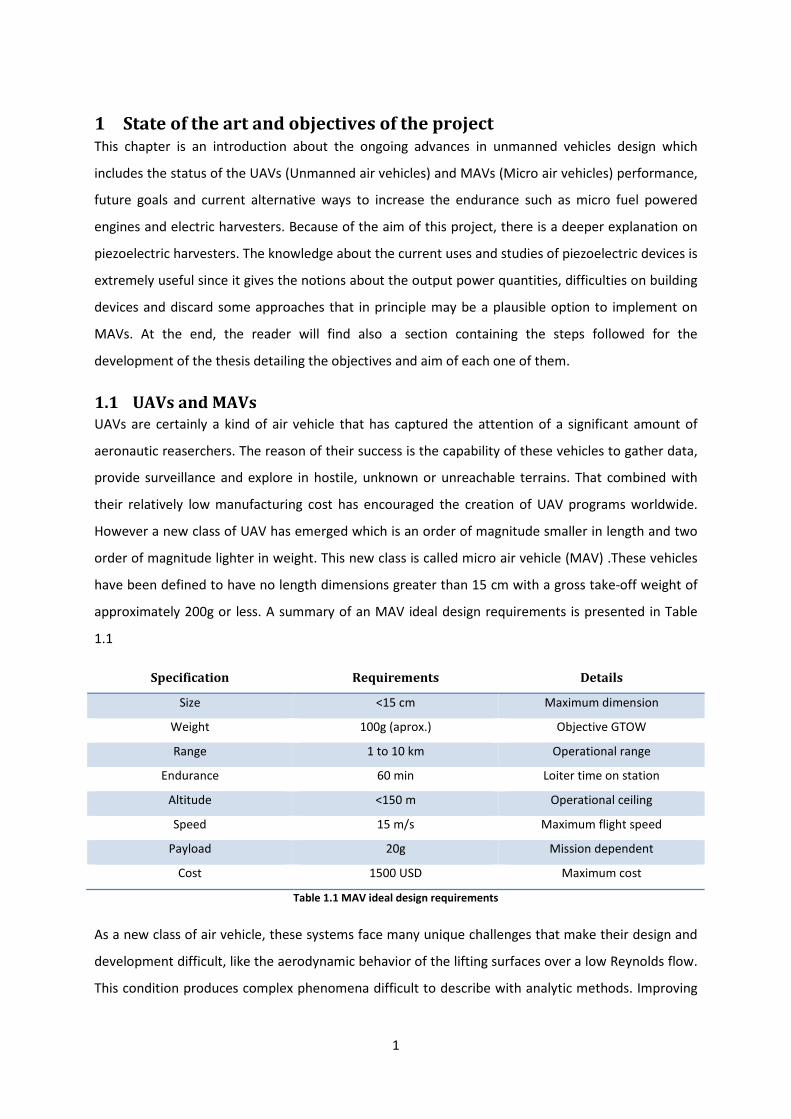
have been defined to have no length dimensions greater than 15 cm with a gross take-off weight of
approximately 200g or less. A summary of an MAV ideal design requirements is presented in Table
1.1
Specification Requirements Details
Size <15 cm Maximum dimension
Weight 100g (aprox.) Objective GTOW
Range 1 to 10 km Operational range
Endurance 60 min Loiter time on station
Altitude <150 m Operational ceiling
Speed 15 m/s Maximum flight speed
Payload 20g Mission dependent
Cost 1500 USD Maximum cost
Table 1.1 MAV ideal design requirements
As a new class of air vehicle, these systems face many unique challenges that make their design and
development difficult, like the aerodynamic behavior of the lifting surfaces over a low Reynolds flow.
This condition produces complex phenomena difficult to describe with analytic methods. Improving

2
the endurance is another major issue concerning the MAV design due to the necessity of improving
the performance for longer missions without penalize on the dimension requirements.
Figure 1.1 Current MAV performance and desired target, courtesy of Pines et al [1]
Specifically focusing on the endurance issue, ongoing projects are trying to build MAVs capable to
flight for more than an hour, which is more than twice the endurance of the current designs
performance. Figure 1.1 shows current projects and the point of ideal requirements, which is also the
ideal target used to achieve the goal of this thesis. Endurance of a vehicle is inversely proportional to
the power required to maintain steady state level which implies the necessity to minimize the power
required to increase the endurance. Compared to full-scaled aircrafts, MAVs use a higher percentage
of propulsion mass. See Figure 1.2 comparing the mass fraction of three different MAVs compared to
a Boeing 767.
Figure 1.2 Mass fractions for different air vehicles, Courtesy of Pines et al [1]
Note how the three micro vehicles use an extra 20% on propulsion mass fraction than the full scale
aircraft while the structure fraction shows the inverse situation, large aircrafts use between 10% and

3
15% more structural mass than the MAVs. This fact leads to think about the use of power sources
able to provide higher energy density_ 92A`aAa.c A 0d or even better, a double function: a structure
able to provide power as well.
1.2 Approaches for extended endurance
There are different approaches to improve the endurance problem; this chapter presents different
options taking a deeper look into electric harvesters. The reader shall take a look at the current
trends to be aware of the effort put in reach better results and to point the variety of alternatives
that are being explored. This may help as well to clarify the aim of the current project and the
motivation on keeping developing solutions for future projects.
1.2.1 Micro-engines
There is a solid base on developing air vehicles based on fossil fuel propulsion. For UAVs, air-
breathing engines are still and option because there are no dimension limitations. Instead, for MAVs
using the same technology become a hard work. Nevertheless, there are current projects working on
the development of micro-scaled1 fuel engines. MIT is currently developing micro-gas turbines of
1& diameter by 3&& thick using semiconductor materials and using the MEMS
(Microelectromechanical systems) technology. These engines are designed to produce 10-20W of
electric power or 0,05-0,1 [ of thrust while consuming under 10 e/ℎ of H2.
The primary application for these systems is to be able of recharging batteries. In general, tens of
watts of electric power are enough to charge many portable devices. Besides, the energy density of a
liquid hydrocarbon fuel is 20-30 times that of the best battery technology so the size of the power
source can shrink simultaneously. If there are other systems that need more power than one single
engine can provide, then several can be used in parallel. One convenient way of implementing this
parallelism would be connect them using a wafer plate as the substrate to integrate the whole
system, e.g. including the interconnecting fuel and control lines on the fabrication wafer. Such a
wafer, 200 mm diameter by 3 mm thick, could produce as much as 10 kW of power. Since its power-
to-weight ratio is so high, one attractive use of such an array would be for distributed, compact,
highly redundant auxiliary power units in air and land vehicles.
Another use for micro-gas turbine engines is vehicle propulsion. The output of a single engine is
sufficient for the micro-aircraft of current interest, with gross takeoff weights of 50-100 g. When
1 The term micro-scale may not be really accurate since the dimensions of the engine are noticeable with the human eye,
however the MEMs technology is used to produce the different elements of the engine, and this is why prefix micro- is
used.

4
more thrust is needed, multiple engines or wafers can be used. A 200 mm diameter wafer may
produce 95 N of thrust. Another advantage of a micro-engine approach to propulsion is that thrust is
truly modular, so one engine design can be used over a wide range of vehicles and thus be produced
in large quantity. Also, an increase in vehicular thrust requirements would be met simply by adding
more engines, rather than the current practice of modifying or redesigning the engine. Figure 1.3
shows the layout of a micro-engine:
Figure 1.3 Micro gas turbine generator cross-section, extracted from [2]
Similarly to the micro gas turbine, there is another device under development: The micro-
bipropellant rocket engine. The engine consists of a regenerative cooled chamber and nozzle, pumps,
controls, and plumbing. The engine configuration is prismatic 2-D structure to be compatible with
current fabrication technology (see Figure 1.4). This requires all of the nozzle expansion to be in-
plane so it is the nozzle exhaust area which limits the engine power that can be fit onto a chip rather
than propellant pumping capability. There are several options for producing much larger thrusts if
needed, including: stacking motors together; placing only the pumps, controls and chamber on a chip
and mating one or more such chips to a conventionally fabricated large exhaust nozzle; or placing
only the pumps and controls on a chip and feeding a conventional chamber and nozzle.
Single engine applications might include spacecraft attitude control and station keeping. Arrays of
20-50 engines could be used for apogee kick. Larger arrays might be used for main propulsion for
very small launch vehicles. In this application, differential throttling across the array could provide
thrust vector control.
Figure 1.4 Micro -bipropellant rocket engine layout, extracted from [2]

5
1.2.2 Solar harvesters
Probably the most used harvesters intended to cover vehicle applications (among other rather more
conventional applications) are the solar harvesters. Its notorious advantages in large scale aerial
vehicles have granted them deeper investigations to achieve better results in new MAV projects until
limits such as create UAVs capable of flying continuously without any other source of energy. The
photoelectric effect is well studied and hence difficult to find quick and reduced cost improvements
to apply on MAVs. However, for aviation projects like MAV or UAV the goal is to design aircrafts that
complement the use of the solar harvesters in order to preserve the gathered energy for situations
where is not possible to use solar arrays. Those situations would be the night time or environment
difficulties such as dense clouds. That is why the majority of the ongoing projects of solar MAVs are
focused in high altitude flights, where the resistance is lower; the atmospheric events such as winds,
clouds and storms are unlikely to happen and the endurance can be increased in great amount if the
aircraft counts on a well planned design. High aspect ratio is then, the common choice when
designing solar powered aircrafts.
The technology is suitable for MAVs too but there are some restrictions that make difficult to use it in
the same ways as UAVs do. The size reduction is one of them; the batteries are small and cannot
store as much energy as larger aircrafts but in daylight operation is a helpful solution for the
endurance issues. The propulsion power makes difficult for these vehicles to fly at high altitudes and
electronic devices like cameras do not have enough capacities to perceive the terrain at long
distances, hence MAVs are forced to flight at low altitudes and are exposed to adverse atmospheric
events which reduce considerably the flight time. Larger panels are needed to achieve the desired 60
min flight time but then more surface is needed which translates into bigger airplanes leaving
consequently the scale of MAV sized vehicles. MAV projects like the HORNET and WASP from DARPA
agency use solar cells on top of the wing but neither of them have report significant results
compared with the rest of MAV models without harvesting systems.
1.2.3 Piezoelectric harvesters
Nowadays, solar/wind harvesters and electric energy seems to be the most common way to collect
energy because of the uses in macroscopic scale. However, the piezoelectricity is becoming a trend
due the multiple uses for the new technologies. That is the case of sensors, the great part of tools for
measuring physical variables such as pressure, speed, temperature, accelerations and other
quantities are based on piezoelectric devices. And more important than the implementation of this
effect is the fact that these harvesters can be “easily” designed with small dimensions thanks to the
MEMS technology.
6
Indeed, to improve the efficiency of devices (not only MAVs) that require small power sources, it is
vital to reduce the mass of the harvesters as well as to provide the highest possible power density.
Piezoelectric materials seem to have enough specific powerg6`to capture small movements, since
currently their main application is to amplify signals of transducers, and produce a voltage that can
be measured but it is not so clear that this energy could be stored with profitable benefits. A lot of
effort and creativity has been put together to find out whether it is a sensible solution or these
applications suit better for other materials rather than piezoelectric.
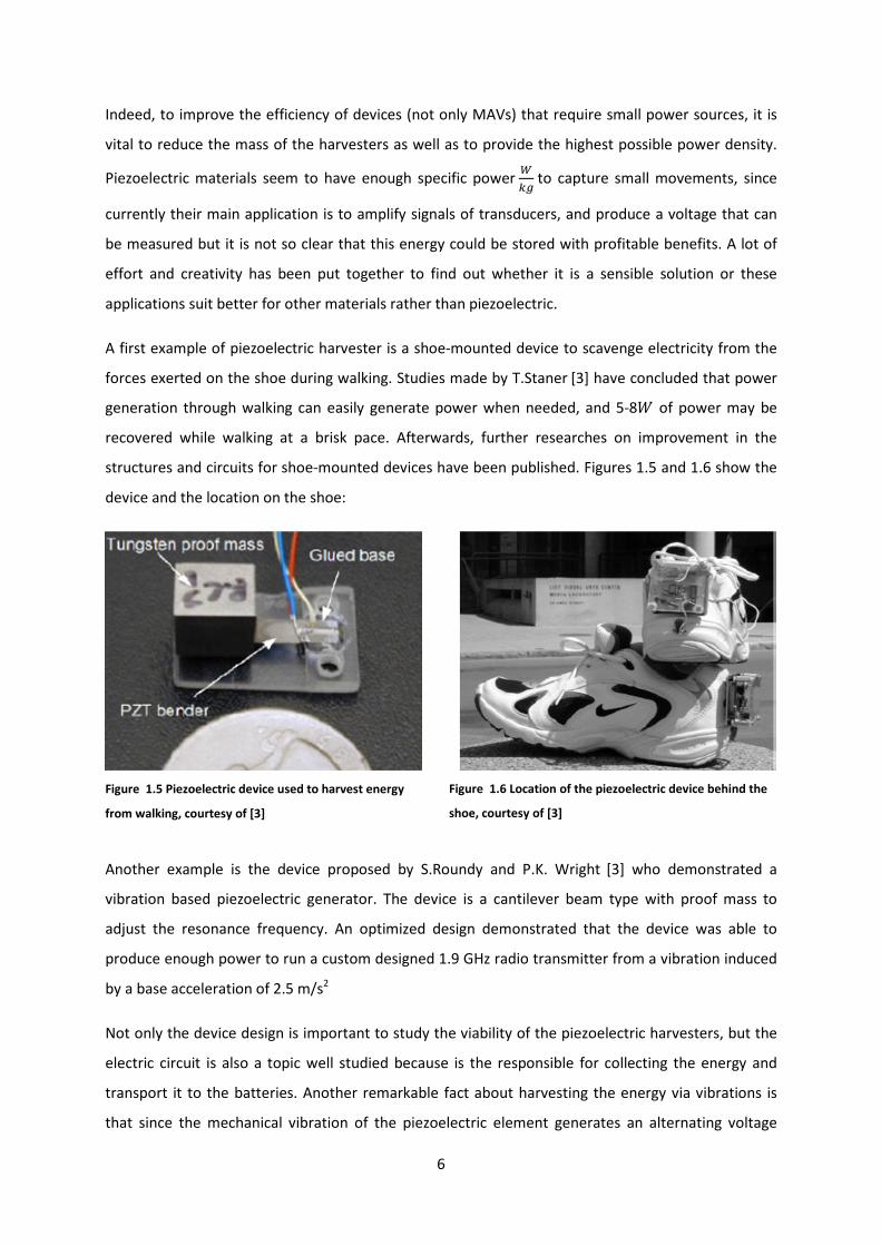
A first example of piezoelectric harvester is a shoe-mounted device to scavenge electricity from the
forces exerted on the shoe during walking. Studies made by T.Staner [3] have concluded that power
generation through walking can easily generate power when needed, and 5-8? of power may be
recovered while walking at a brisk pace. Afterwards, further researches on improvement in the
structures and circuits for shoe-mounted devices have been published. Figures 1.5 and 1.6 show the
device and the location on the shoe:
Figure 1.5 Piezoelectric device used to harvest energy
from walking, courtesy of [3]
Figure 1.6 Location of the piezoelectric device behind the
shoe, courtesy of [3]
Another example is the device proposed by S.Roundy and P.K. Wright [3] who demonstrated a
vibration based piezoelectric generator. The device is a cantilever beam type with proof mass to
adjust the resonance frequency. An optimized design demonstrated that the device was able to
produce enough power to run a custom designed 1.9 GHz radio transmitter from a vibration induced
by a base acceleration of 2.5 m/s2
Not only the device design is important to study the viability of the piezoelectric harvesters, but the
electric circuit is also a topic well studied because is the responsible for collecting the energy and
transport it to the batteries. Another remarkable fact about harvesting the energy via vibrations is
that since the mechanical vibration of the piezoelectric element generates an alternating voltage

7
across its electrodes, most of the proposed electrical circuits include an AC-DC converter to provide
the electrical energy to its storage device, as illustrated in Figure 1.7.
Figure 1.7 Standard interface circuit
Researches such as the proposed by Guyomar et al [4], Lefeuvre et al [5]and Badel et al [6] have
developed a new flow optimization principle based on the extraction of the electric charge produced
by a piezoelectric element, synchronized with the mechanical vibration operated at the steady state,
as shown in Figure 1.8. They have claimed that the harvested electrical power may be increased by as
much as 900% over the standard technique.
Figure 1.8 Switch Synchronized charge extraction
A similar model that has also been studied and its performance analyzed, is known as synchronized
switch harvesting on inductor (SSHI) (see Figure 1.9) and seems to present a similar behavior to that
of the electrical response produced by the standard interface model in a strongly coupled
electromechanical system operated at short circuit resonance.
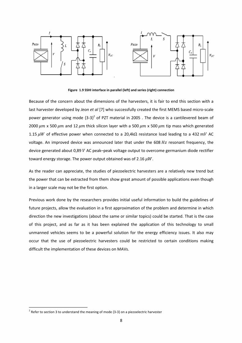
8
Figure 1.9 SSHI interface in parallel (left) and series (right) connection
Because of the concern about the dimensions of the harvesters, it is fair to end this section with a
last harvester developed by Jeon et al [7] who successfully created the first MEMS based micro-scale
power generator using mode 3-32 of PZT material in 2005 . The device is a cantilevered beam of
2000& x 500& and 12&thick silicon layer with a 500& x 500& tip mass which generated
1.15? of effective power when connected to a 20,4kΩ resistance load leading to a 432&= AC
voltage. An improved device was announced later that under the 608hG resonant frequency, the
device generated about 0,89= AC peak–peak voltage output to overcome germanium diode rectifier
toward energy storage. The power output obtained was of 2.16?.
As the reader can appreciate, the studies of piezoelectric harvesters are a relatively new trend but
the power that can be extracted from them show great amount of possible applications even though
in a larger scale may not be the first option.
Previous work done by the researchers provides initial useful information to build the guidelines of
future projects, allow the evaluation in a first approximation of the problem and determine in which
direction the new investigations (about the same or similar topics) could be started. That is the case
of this project, and as far as it has been explained the application of this technology to small
unmanned vehicles seems to be a powerful solution for the energy efficiency issues. It also may
occur that the use of piezoelectric harvesters could be restricted to certain conditions making
difficult the implementation of these devices on MAVs.
2 Refer to section 3 to understand the meaning of mode 3-3 on a piezoelectric harvester
9
1.3 Objectives of the project
In view of the previous information, this report has been structured following a typical design
scheme. That is, identifying the needs of the problem, bounding key parameters to create a basic
layout of the solution and testing the proposed concept (looping if necessary) until it is adjusted for
an optimal performance. Each chapter has particular objectives; the achievement of these objectives
provides advances in the study. In the end, every partial result and study will lead to the final
solution and conclusions. The approach described above will be developed in the next chapters.
The following chapter to proceed with the identification of the problem requirements; the goal here
is to bound the performance of the harvester in order to adapt it to the problem specifications.
Subsequently, two chapters include the modeling of the MAVs endurance and the piezoelectric
behavior of the harvester with a mathematical approach, giving the basis to carry out simulations on
future harvester designs and connecting both the parameters aimed to be improved and the
piezoelectric inputs. At last, a chapter to describe the results of the design process, showing how the
tests were performed and how the final harvester evolved since the first concept until the last
version.
An extra chapter is also dedicated to a theoretical approach on the design of an external harvester.

10
2 Design requirements The design of piezoelectric harvesters is subjected to several restrictions because they depend on
external factors to collect the energy. The current work aims to install them into MAVs to take
advantage of the vibrations. Nevertheless, vibrations are not the only important aspect to achieve an
optimal design, materials, layout and/or configuration of the device as well as the mission to be
performed by the MAV could affect the performance of the harvester.
The next lines will show which are the key parameters needed to make the preliminary designs and
check the viability of using piezoelectric harvesters to improve MAVs performance.
2.1 MAV design conditions
An important requirement of the project is fix the design conditions at cruise stage of the flight which
is most of the mission time (since MAV are almost exclusively designed for reconnaissance missions).
Their small size and limited weight cannot allow them to perform complex tasks but this limitation is
actually an advantage because the harvester will be working during the majority of the mission at
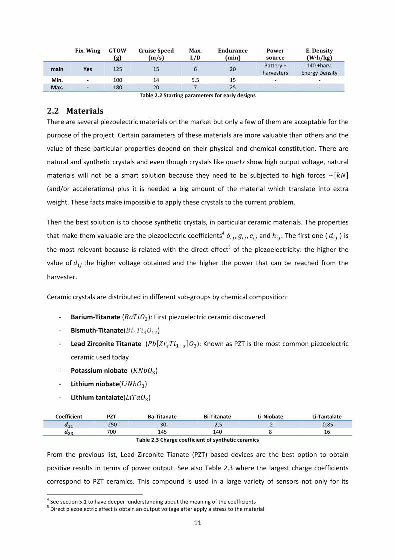
design conditions. Table 2.1 shows some MAV models and their respective performance parameters.
Properties Black Widow Hoverfly LUMAV MicroStar Microbat MICOR
Fixed wing Yes No No Yes Yes No
GTOW (g) 80 180 440 110 10.5 10.3
Cruise Speed (m/s) 13.4 15-20 5 13.4-15.6 5 2
Max L/D 6 N/A3 N/A 6 N/A 5
Endurance (min) 30 13.2 20 25 2.25 3
Power Source Li-ion Batteries Li-ion
Batteries
2-stroke IC
engine
Li-ion
Batteries
NiCad N-50
cells (Sanyo)
Li-ion
Batterie
s
Energy density
(W·h/kg) 140 140
5500
methanol 150 100 150
Table 2.1 MAV performance properties [1]
Fixed wing MAVs are the priority because this project is focused on this configuration. Notice the
similarities between MicroStar and Black Widow; their parameters are the base to begin the design
because they are able to actually perform a mission. Microbat has a remarkably reduced endurance
and low weight that makes him stay out of the MAV requirements. Comparing performance with
both fixed wing and hover MAVs two different group can be made, that is by comparing the flight
time. In fact, endurance between 10 and 30 minutes are low but acceptable values to work with,
while flight times between 2 and 5 minutes are not. This means that preliminary values for the rest of
the performance parameters are chosen in accordance to endurance values around 20 minutes.
Table 2.2 shows the values accepted for a starting point with some thresholds to adjust if it is
necessary.
3 N/A: Not available
11
Fix. Wing GTOW
(g)
Cruise Speed
(m/s)
Max.
L/D
Endurance
(min)
Power
source
E. Density
(W·h/kg)
main Yes 125 15 6 20 Battery +
harvesters
140 +harv.
Energy Density
Min. - 100 14 5.5 15 - -
Max. - 180 20 7 25 - -
Table 2.2 Starting parameters for early designs
2.2 Materials
There are several piezoelectric materials on the market but only a few of them are acceptable for the
purpose of the project. Certain parameters of these materials are more valuable than others and the
value of these particular properties depend on their physical and chemical constitution. There are
natural and synthetic crystals and even though crystals like quartz show high output voltage, natural
materials will not be a smart solution because they need to be subjected to high forces ~j
12
piezoelectric properties but for the pyro electric effect and its large dielectric constant. It is usually
not used in its pure form, rather it is doped with either acceptor dopants, which create oxygen
(anion) vacancies, or donor dopants, which create metal (cation) vacancies and facilitate domain wall
motion in the material. In general, acceptor doping creates hard PZT while donor doping creates soft
PZT. Hard and soft PZT's generally differ in their piezoelectric constants. Piezoelectric constants are
proportional to the polarization or to the electrical field generated per unit of mechanical stress, or
alternatively is the mechanical strain produced per unit of electric field applied. In general, soft PZT
has higher piezoelectric constants, but larger losses in the material due to internal friction. In hard
PZT, domain wall motion is pinned by the impurities thereby lowering the losses in the material, but
at the expense of a reduced piezoelectric constant. The bibliography includes catalogs of PZT model
materials that show their properties [8] [9] [10] [11].
The other materials listed before are also commonly used but each one for specific applications. That
is one of the main differences with PZT, these materials cannot be as easily adapted to other
applications. Barium titanate sometimes replace PZTs as a dielectric materials, bismuth titanate has
its best performance in application at high temperatures where is able to reach similar charge
coefficients to those of the PZTs. Lithium niobate is used extensively in the telecoms market and is
the material of choice for the manufacture of surface acoustic wave devices, those surfaces are used
to build filters or DC to DC converters. Sometimes lithium niobate can be replaced with lithium
tantalate as well. Finally Potassium niobate has nonlinear optical coefficient properties, making it
common in the manufacture of lasers. The cost of these materials is similar except for those with
high technology applications like potassium niobate. In terms of availability and manufacturing
spectrum again PZT is the most advantageous material counting on different doped versions, plate
dimensions or particular use for MEMS applications
Designing a harvester choosing only one kind of ceramic material would be simplistic but try every
ceramic crystal would take a lot of time and effort that might be unnecessary. That is why in this
section PZT has been discussed to be the best option. In the results, the reader will find graphics
where different PZTs are compared to find an optimal output response.
2.3 Piezoelectric modes
There are two configurations considered in this project to design piezoelectric harvesters, depending
on the direction between the strain applied and the direction of the electric field. The first
configuration is called 3-1 and indicates that strain and electric field vectors are perpendicular. The
second configuration is 3-3, which indicates that both electric and strain vectors are parallel.
13
There are differences when deciding between 3-1 and 3-3 configurations for a device design but
in general the piezoelectric effect is larger for 3-3 mode, as for most piezoelectric devices the ratio
1vv1vw ~2.4 . [12]
At first glance, 3-3 mode seems to be the best option but there are some features that would make
3-1 mode a more successful choice. The first feature is the complexity of the manufacturing
process, if there is a chance to use mode 3-1 and obtain outputs that satisfy the power
requirements then there is no need to increase the cost of the product. Another issue is the model
used to simulate the behavior of mode 3-3, some assumptions have been made to simplify the
equations and therefore the results obtained may not be as accurate as desired but it provides the
order of magnitude, which is vital to know if this technology can be applied on MAVs. The following
lines explain the layouts of both modes.
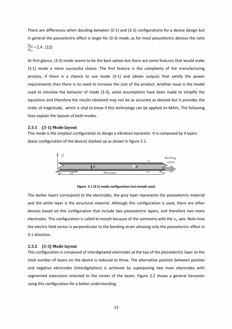
2.3.1 3-1 Mode layout
This mode is the simplest configuration to design a vibration harvester. It is composed by 4 layers
(basic configuration of the device) stacked up as shown in figure 2.1.
Figure 2.1 3-1 mode configuration (uni-morph case)
The darker layers correspond to the electrodes, the grey layer represents the piezoelectric material
and the white layer is the structural material. Although this configuration is used, there are other
devices based on this configuration that include two piezoelectric layers, and therefore two more
electrodes. This configuration is called bi-morph because of the symmetry with the Foaxis. Note how
the electric field vector is perpendicular to the bending strain allowing only the piezoelectric effect in
3-1 direction.
2.3.2 3-3 Mode layout
This configuration is composed of interdigitated electrodes at the top of the piezoelectric layer so the
total number of layers on the device is reduced to three. The alternative position between positive
and negative electrodes (interdigitation) is achieved by superposing two main electrodes with
segmented extensions oriented to the center of the beam. Figure 2.2 shows a general harvester
using this configuration for a better understanding.

14
Figure 2.2. Interdigitated electrodes in a piezoelectric harvester (yellow components)
The green layer represents the piezoelectric material and the grey one is the structure layer. Now is
easier to see that both electric field and strain act in the same direction, however the electric field
does not act as a straight line because the disposition of the electrodes face the surface towards the
piezoelectric layer instead of facing the complementary electrode. Looking at figure2.3 it is clear that
the electric field bends to in order to find the way to the other electrode. This fact makes the
electromechanical modeling of this mode quite difficult.
Figure 2.3 Transversal view of a harvester in 3-3 configuration
This is why certain assumptions are introduced as well as a variation of the electrode configuration to
obviate theoretical problems. When working with this mode it will be assumed that the region of the
piezoelectric element under the electrode is electrically inactive, whereas the section between the
electrodes utilizes the full mmeffect. Physically, these considerations translate to figure 2.4.
Figure 2.4 3-3 mode layout assuming simplifications

15
2.3.3 Comparison between modes
Some bibliographical research [3] [12] has shown that even though mode 3-3 seem to enlarge the
output of the harvester, the experimental performance results show a different behavior for some
variables. In an experiment described by Wu et al [3], two MEMS generators, each one with a
different configuration, were excited at 2g acceleration level. The measurements are summarized in
table 2.3:
Mode yz| ~ ~ 3-1 255.9 Hz 150 kΩ 2.099 ? 2.415 =ara 1.587 =ara
3-3 214.0 Hz 510 kΩ 1.288 ? 4.127 =ara 2.292 =ara
Table 2.4 Results comparing the performance between piezoelectric modes 3-1 and 3-3
For the same dimensions of the beam the output power for the 3-3 mode piezoelectric MEMS
generator was smaller than that for the 3-1 mode piezoelectric MEMS generator. This was due to
the PZT material of the 3-3 mode device which was poled using the interdigitated electrodes and
which results in a non-uniform poling direction because the piezoelectric under the electrode is a
region affected by the electric field. The material under the electrodes was not used because it was
not poled correctly. Furthermore, the further the distance from the surface of the PZT material, the
less effective the poling electric field strength will be. This causes an efficiency drop for the 3-3
mode piezoelectric MEMS generator when compared to the 3-1 mode piezoelectric MEMS
generator. Nevertheless, the output voltage of the 3-3 mode piezoelectric MEMS generator was
higher than that of the 3-1 mode piezoelectric MEMS generator and easily adjusted by the gap of
the interdigitated electrodes under the same dimensions of the beam shape.
Talking about generators at a higher scale means that mode 3-3 efficiency would be even lower
than that for the MEMS generator described in the previous lines. Then, designing a harvester to suit
an MAV with this mode does not have a clear benefit over mode 3-1. For this reason, in the
development of this thesis only mode 3-1 is considered in the design of the harvester. Besides, the
fabrication process cost of 3-3 configuration is higher than the 3-1 mode which means an extra
expense with the only benefit of being able to adjust the output voltage in a more controlled way.
But controlling the voltage will not be an important feature if the necessary power cannot be
assessed to improve the MAV endurance. Mode 3-3 would be a good improvement in advanced
stages of a possible harvester design where more accurate conditions are needed to perform an
optimal output.

16
3 MAVs endurance In order to design a device to improve MAV’s endurance, there must be a criterion to evaluate how
adding new components to a vehicle affects its maximum flight time. In fact, there are certainly
known expressions to estimate the endurance of an aircraft such as the Breguet equation. This
chapter is dedicated to find a similar expression for an air vehicle powered by electric energy with or
without energy harvesting systems. This allows to compare whether the addition of energy
harvesters improve or worsens the original MAV’s design.
The method used in this thesis is based in (Anton, S. R)6 [13, 14]. The expression (3.1) is valid for
electric powered aircraft in a steady level flight.
89 = J
?Dmp − .@ AB T>4m2p opT>4m2p
op J
(3.1)
Where 89 represents the endurance, is the energy from the batteries, ?Dis the total weight of
the MAV, .@ AB is the power provided by a harvester, T>represents the air density, 4stands for the
MAV wing surface , and are the lift and drag coefficient respectively, and finally Jand Jstand for the efficiency of the batteries and the propulsion system respectively.
3.1 Endurance formulation
The formulation can be derived by considering a basic aerodynamic model to describe the flight of an
aircraft as a balance between the energy required for steady, level flight and the energy available
from all power sources.
In steady level flight, thrust5equals to dragand lift$equals to weight?: 5 = (3.2)
$ = ? (3.3)
The thrust required can be expressed as a function of the weight and the MAV’s aerodynamic
efficiency by combining both previous equations:
5 = ?$/ (3.4)
Recall that the ratio $/can be expressed as a ratio of / since:
6 The original development of the theory is presented by Thomas et al [21] and cited by Anton, S.R.
17
$ =
12 =>pT>412 =>pT>4
= (3.5)
On the other hand the required power for cruise configuration is given by:
.7 = 57=> (3.6)
Substituting equation (3.4) into (3.6) yields to:
.7 = ?/ => (3.7)
Velocity can be written as well in terms of the weight and lift coefficient by using the relation$ =? = op=>pT>4. Solving for=>:
=> = 2?T>4 (3.8)
Then the power required for steady level flight becomes:
.7 = 1J ?/ 2?
T>4 = 1J 2?mpT>4m (3.9)
Note that the term Jhas been added to introduce the efficiency (to convert electric energy into
mechanical power) of the aircraft propeller and motor. Other losses may be considered if a careful
breakout of this term was made: namely losses due to the speed controller and losses between
connections inside the propulsion system. However, when developing the final equation this term
will be vanished so the precision does not need to be highly accurate at this stage.
Endurance is introduced using the physics definition of power.7 = /8, where refers to energy
and 8refers to time or endurance 89 as it will be called from now on. The energy available in an
electric aircraft can be written as a sum of the contribution of the battery power supply plus the
extra harvesting devices:
B " = J + . AB89 (3.10)
Balance between energy available and the power required for a leveled flight leads to:
18
89 = B ".7 = J + . AB89?m/p T>4m2p
o/pJ (3.11)
Solving for89 yields to the original expression shown at the beginning of this chapter:
89 = J
?Dmp − .@ AB T>4m2p opT>4m2p
op J
(3.12)
3.2 Normalized endurance
When applying expression (3.12) it is useful to compare the results of the endurance of an MAV with
the ones obtained in the same vehicle without any kind of harvesters. To do so, the endurance may
be expressed as an increment value that can also be normalized with the resulting value from a non-
harvesting MAV.
A linear series Taylor expansion of89 about the point.@ AB = 0can be used to formulate the
normalized change in flight endurance. By taking the aerodynamic terms in (3.12) as a constant:
= T>4m2p
op J (3.13)
The flight time is expressed as:
89 = J ?Dmp − .@ ABro J (3.14)
Now applying the Taylor series expansion for a first order approximation:
F, , G ≈ F, , G + F,,, F − F + ,,, − +
G,,, G − G (3.15)
The endurance can be estimated as:
Δ89 = 89 − 89 ≈ 89J ΔJ +89?D Δ?D + 89.@ AB Δ.@ AB (3.16)
Δ89 ≈ ?Dm/p ΔJ −32
J?D /p Δ?D + Jp
?Dm Δ.@ AB (3.17)
Now the normalization is made as explained before with the expression of endurance for a non-
harvesting MAV. If .@ AB = 0is set in equation (3.12):
19
89 = J?Dm/p (3.18)
And dividing expression (3.17) by (3.12) the normalized change in flight time can be written as:
Δ8989 ≈ ΔJJ − 32 Δ?D?D + Δ.@ ABJ/89 (3.19)
This equation can also be written in terms of changes in mass by decoupling the weight in different
terms:
?D = ? + ?CD + ?@ AB (3.20)
And using some relations to define the terms in equation (3.19) as well:
= & (3.21)
? = &e (3.22)
.@ AB = \@ AB&@ AB (3.23)
J/89 = \ B& (3.24)
Where:
- And&are specific energy of the battery _ ¡6`d and the mass of the battery respectively.
- \@ AB And &@ AB is the specific power of the harvester_g6`d and the mass of the harvesting
system respectively.
- \ Bis the specific power supplied by the battery in the non-harvesting design i.e.\ B =J/89&
Finally the resulting expression is written as:
Δ8989 ≈ Δ&& − 32 Δ& + Δ&CD + Δ&@ AB&D + \@ ABΔ& AB\ B& (3.25)
where&Dis the total mass of the aerial vehicle. The simple aerodynamic model used in the
derivation naturally adds several assumptions about the flight of the aircraft and the ambient
environmental conditions, namely imposing constant conditions. The formulation, however, can be
used to provide the effects of adding energy harvesting systems to electric powered UAVs and MAVs.

20
4 Embedded piezoelectric device approach
The embedded piezoelectric beam is a device located inside the structure of the MAV that is meant
to vibrate due to the surrounding wind flow over the fuselage. The device will be coupled as a
cantilevered beam in order to transmit the vibrations from the structure to the beam. The
electromechanical method used to analyze the behavior of a concept device is based in the energy
method approach proposed by duToit [12]. This chapter will include a developed explanation of this
method.
The harvester layout is formed by a bi-morph7 cantilevered beam including 4 electrodes and a
structural layer and two piezoelectric layers, as shown in figure 4.1:
Figure 4.1 Layout of the internal harvester. Black layers represent electrodes, white structural material and grey
piezoelectric material
4.1 Piezoelectric constitutive equations
The piezoelectric effect is the combination of the mechanical and electrical behavior of a material.
Therefore is imperative to present the mathematical description of such materials in order to
develop the electromechanical model for the bending beam approach. On one hand, the Hooke’s law
relates the mechanical stress5 and strain4: 4 = ]5 → 4"# = ]"#6 56 (4.1)
Where ]"#6is the compliance or the inverse stiffness.
On the other hand, the expression relating the electric field with the electric displacement is defined as:
= K → " = K"# # (4.2)
Where K"#is the electric permittivity
7 See annex A for deeper information about Bi-morph configuration and its implications when connecting the
electrodes of the different layers.
21
These two matrix expressions can be combined into coupled equations that adopt the form:
4 = ]5 + 0 → 4"# = ]"#6 56 + 6"#6 (4.3)
= 5 + εE → " = "#6 5#6 + K"## (4.4)
These can be written in matrix form as it is shown in expressions (4.5).
¥4¦ = j]9k¥5¦ +j0k¥¦ ¥¦ = jk¥5¦ + jKDk¥¦ (4.5)
This expression is called the (S-D) form of the coupled equations, being S and D the dependent
variables. jk and j0k represent the matrix of the direct effect (application of stress to get a voltage
output) and converse piezoelectric effect (application of a voltage to induce a stress in the material).
The superscript denotes strain applied at zero or constant electric field and superscript 5 denotes
zero or constant stress.
It is possible to write the same expression in the (T-D) form defining stress and electric displacement
as dependent variables:
¥5¦ = j9k¥5¦ +jk¥¦ ¥¦ = jk¥5¦ + jKCk¥¦ (4.6)
Here j9krepresents the stiffness matrix and jkis the piezo-electrically induced stress tensor as it
relates the stress with to the electric field.
The described model of this project is reduced to the 1D case (bending movement only) and so the
equations will be reduced to a simplified expression presented below for both T-D and S-D systems.
§5mm¨ = ©mm9mm−mmKmmC ª §4mm¨ (4.7)
§4mm¨ = ©]mm9mmmmKmmD ª §4mm¨ (4.8)
When applying these equations, the poling direction of the material has to be taken into account
because depending on it, the sign of some terms change to be consequent with the reaction on the
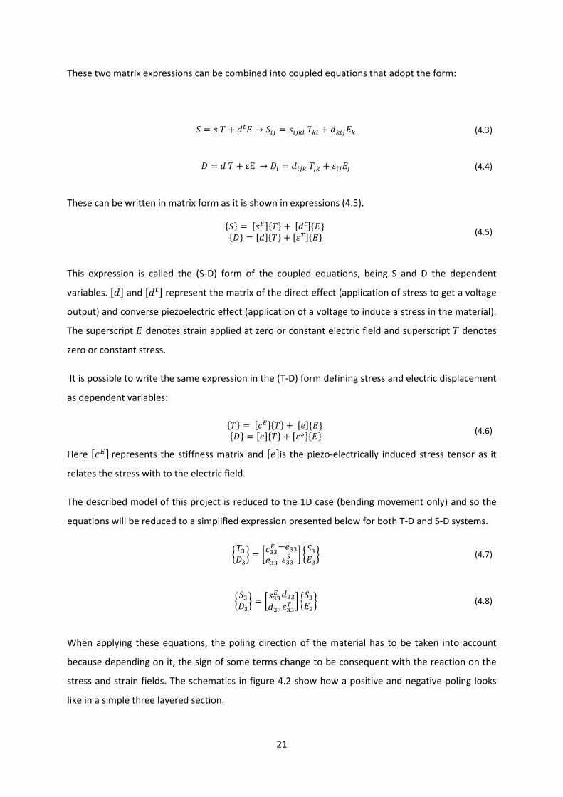
stress and strain fields. The schematics in figure 4.2 show how a positive and negative poling looks
like in a simple three layered section.
22
Figure 4.2 Positive poling (left) and negative poling direction (right). Black layers represent piezoelectric material being
used as electrodes
All the nomenclature is already known except for . which is the poling direction. Note that the
difference between the two poling configurations is the relation of the pole with the global
coordinate, the poling direction determines the local coordinates and therefore there is a change in
the constitutive equation if the global and the local coordinates are oriented in opposite directions.
These changes are reflected in the following equations.
§5mm¨ = © mm9−mmmmKmmC ª §4mm¨ (4.9)
§4mm¨ = © ]mm9−mm−mmKmmD ª §4mm¨ (4.10)
Now these equations have to be added with the mechanical theory in order to build a coupled model
so the displacements can be related with the voltage and power. Next section is dedicated to
develop the method use to reach the final model.
4.2 Electromechanical model
4.2.1 Governing equations
As discussed on the introduction the model is based on the energy method approach8. The model
starts with the generalized form of the Hamilton’s principle for an electromechanical system where
magnetic terms are neglected:
« jl56 − : +? + l?k8 = 00p0o (4.11)
Where:
- 56 is defined as the kinetic energy
- : represents the internal potential
- ? defines electrical energy
- ? is the applied external work
8 The analysis of the model is based on [12] and adapted from Hagood et al [20]

23
The individual energy terms are defined as follows:
56 = 12 « TC;0 ¬ ;¬ =C®+12 « T ;0 ¬ ;¬ =¯
(4.12)
: = 12 « 40 5=C®+12 « 40 5=¯
(4.13)
? = 12 « 0 =¯ (4.14)
In both 56 and :there are two contributions due to the structural layer (subscript S) and the
piezoelectric layer/s (Subscript P). Electrical energy is only taken into account in piezo-layers and the
contribution due to fringing fields in the structure and free space is neglected. The terms ;, ;¬ represent the relative displacement ;F, 8and the successive time derivatives. The rest of the
terms (5, , 4, ) are known from the coupled piezoelectric equations.
The term involving the external work is computed with the next expression:
l? = °l;668 + °lφ²(# 2³#o
26o (4.15)
It is defined as a combination of two contributions. The first contribution is due to the external forces 6 and mechanical displacements;F6, 8 on the device counted as discrete forces ' applied at a
certain pointF6. The second contribution is due to the electrical potential Q# = Q´F#, 8µ and a
certain amount of charges'(, extracted at discrete electrodes with position F# The next step is the substitution of equations (4.12) to (4.14) into (4.11) leading to the developed
equation:
« ¶l ·12 « TC;0 ¬ ;¬ =C®+12 « T ;0 ¬ ;¬ =¯
− 12 « 40 5=C®−12 « 40 5=¯
0p0o
+ 12 « 0 =¯¸ +°l;668 + °lφ²(# 2³
#o26o ¹ 8 = 0
(4.16)
24
The number of variables is reduced using the coupled expressions of the piezoelectric effect. In the
definition of the device9 the local coordinates are superposed to the global ones, therefore the poling
direction chosen in the substitution is the positive alternative, that is, the system provided in
expression (4.7).
« ·« TCl;0 ¬ ;¬ =C®+ « T l;0 ¬ ;¬ =¯
− « l404=C®− « l40 9 4=¯
0p0o
+ « l40 0=¯+ « l0 4=¯
+ « l0 KC=¯+°l;668 +°lφ²(# 2³
#o26o ¸ 8 = 0
(4.17)
Please note that (T – D) form has been used in the substitution because then it is easier to continue
developing and simplifying the equations.
At this point three assumptions are introduced:
- Rayleigh – Ritz procedure [12]:
The displacement of a structure is written as the sum of ')individual mode shapes (RA"F), multiplied by a generalized mechanical coordinate )"8. Since only bending movement is
considered the only displacement allowed is on Z axis along the longitudinal direction:
;F, 8 = GF , 8 =°RA"F )"8 = RAF )82A"o
(4.18)
- Euler Bernoulli beam theory [12]:
Allows the axial strain in the beam to be written in terms of the beam neutral axis
displacement and the distance from neutral axis as:
4F, 8 = −F0 lpGF , 8lF p = −F0RAºº)8 (4.19)
- Constant electric field across the piezoelectric [12]:
Although the constant nature of the electric field considered in the device, the electric
potential for each of the '( electrode pairs can be written in terms of a potential distribution
RB#and the generalized electrical coordinate <#8 9 Refer to figures 4.1 and 4.2

25
QF, 8 = °RB#8<#8 = RB<82³#o (4.20)
Note that prime signs on RA denote derivative with respect to the axial positionF . The substitution of these definitions into the main equation (4.17) yields to:
« ·« Tl)0¬ RA0 RA)¬ =®+ « Tal)0¬ RA0 RA)¬ =¯
− « l)0−F0RAºº0 −F0RAºº)=C®0p0o
− « l)0−F0RAºº0 9 −F0RAºº)=¯+ « l)0−F0RAºº0 0−»RB<=¯
+ « l<0−»RB0 −F0RAºº)=¯+ « l<0−»RB0 KC−»RB0<=¯
+°l)60 RA,60 6 + °lv²0 RB,#0 (# 2³#o
26o ¸ 8 = 0
(4.21)
Using integration by parts and grouping terms by factors l)0and l<0two governing equations are
obtained:
− « RA0 TQA )½ =®
− « RA0 T QA)½ =¯
− «−F0RAºº0 −F0RAºº)=C®
− «−F0RAºº0 9 −F0RAºº)=¯
+ «−»RB0 −F0RAºº)=¯
+°QA,60 6 = 02
"o
(4.22)
«−F0RAºº0 0 −»RB<=¯
+ «−»RB0 KC−»RB0<=¯
+°RB,# (# = 02³
#o (4.23)
Each of these terms is defined as mass %stiffness , coupling Θ and capacitive matrices
as showed in the following equations:
% = « RA0 TQA)½ =®
+ « RA0 T QA )½ =¯
(4.24)
= «−F0RAºº0 −F0RAºº)=C®
− «−F0RAºº0 9 −F0RAºº)= ¯
(4.25)
26
Θ = «−»RB0 −F0RAºº)=¯ (4.26)
= «−»RB0 KC−»RB0<=¯ (4.27)
The final governing equations are:
%)½ + ) − Θ< =°QA0 F6682"o (4.28)
Θ0) + < = −°RB,#´F#µ(#82³#o (4.29)
A base excitation will be the input when applying these equations. To represent the beam’s inertial
load from this excitation, the structure is discretized into ' elements of length F and the local
inertial load is applied on the !0@ element, or6 = &6ΔF E½ . This results in ' discrete loads. &6
Is the element mass per length. The loading is summed for all the elements. In the limit ofΔF →F , the summation reduces to the integral over the structure length and a mass per length
distribution is used, &F . For simplicity, it has been assumed here that the beam cross-section is
uniform in the axial direction so that&F = & = +']8'8. The forcing vector on the right side
of expression (4.28) is then defined as:
= «&F QA0 F
= &«QA0 F
(4.30)
Mechanical damping is added through the addition of a viscous damping term, C, to equation (4.28)
to obtain (4.31). When multiple bending modes are investigated, a proportional damping scheme is
often used to ensure uncoupling of the equations during the modal analysis.
The right hand side of eq. (4.29) reduces to a column vector,( of length '( (the number of electrode
pairs) with element values(D_(D = ∑ (#2³#o d. This equation can be differentiated with respect to
time to obtain current. The current can be related to the voltage, assuming that the electrical loading
is purely resistive, since< = = 1³10.

27
After substituting in both governing equations one get:
%)½ + )¬ + ) − Θ< = E½ (4.31)
Θ0) + < + ( = 0 (4.32)
4.2.2 Modal analysis: Simple bending beam
The previous section has shown that governing equations for a piezoelectric beam can be written in
terms of the mechanical displacement assuming a function QA that describes the shape of the beam
and it is a valid solution to the mentioned equations as well.
Dynamic Euler-Bernoulli beam theory is used to find the modal solution. [12]
pFp
p;Fp = −&p;8p + (F (4.33)
Remember that stiffness is considered constant because the beam is homogeneous along the
x-axis.
In the absence of a transverse load,(F,the free vibration equation is obtained. This equation can
be solved using a Fourier decomposition of the displacement into the sum of harmonic vibrations of
the form
;F, 8 = RAF )8 = jQFr"¿0k (4.34)
WhereP, is the vibration frequency. Then for each value of the frequency, an ordinary differential
equation can be solved:
RÀAN −&PNpQAN (4.35)
Please note that the equation (4.33) has been modified into expression (4.35) to include the term of
natural frequencyPNin order to find the different mode shapes of the beam. [Refer to a generic
mode shape.
And the general solution for the above equation (4.35) is:
QAN = o sinhMNF + p coshMNF + m sinMNF + n cosMNF (4.36)
Where _ÇÈÉ dÊ = ËÌÊÍ is a parameter defined for convenience due to the form of expression (4.35).

28
o, p, m, n are constants solved by applying the boundary conditions to a particular case. The
proposed device is a cantilevered beam without any external force applied on the structure. Thus the
boundary conditions are:
- No displacement nor rotation at fixed end
QAN, = 0QANF , = 0 (4.37)
- Null moment and shear force at the free end
pQANFp , = 0 mQANFm , = 0 (4.38)
The solution of these constants is unique for a set of boundary conditions but the displacement
depend on the frequency which at the same time define the mode shape of the beam.
Solving the system to determine the constants leads to the well-known transcendental expression:
coshMN$ cosMN$ + 1 = 0 (4.39)
Thus by using numerical methods, the mode shapes QN and the natural frequencies ÌÈ are found:
Q2A = ÎcoshMNF − cosMNF + coshMN$ + cosMN$ · sinMNF − sinhMNFsinMN$ − sinhMN$ Ð (4.40)
Where: ÌÈ = ÇÈÑÍË and is an arbitrary constant defining an upper value of the tip displacement.
A fixed value of this constant is not possible to establish so the criterion in this case will be to
consider a maximum value set at Q2A$ = 2
Next step is find the values of %, , Ò, and expressed in eq. (4.24) to (4.27).
At this point, voltage<, intensity, tip displacement)and power./0 are the output
variables that will be used to design the optimal piezoelectric device after solving the governing
equations of the previous section. To do it, the following assumptions have been considered so this
way the governing equations can be reduced to a scalar form.
- QA2 = QAoonly the first bending mode is taken into account
- Only one electrode pair
The governing equations form a second order system and for this reason they can be written as
follows:
29
)½ + 2WcPo) + V%< = − E%½ (4.41)
V)¬ + <¬ + 1 < = 0 (4.42)
where the factors H = Po, Lp = ÓÔÕÖ×and Ω = ØØw have been defined for convenience:
- His a dimensionless time constant.
- Lpis a structure/system electromechanical coupling coefficient
- Ω is the ratio between the excitation Pand the first mode frequencyPo
Using Laplace transforms, the governing equations can be evaluated and the output magnitudes can
be determined:
Ù ) E½ Ù = 1 Ú1 + HΩpÚj1 − 1 + 2WcHΩpkp + j2Wc + ¥1 + Lp¦HΩ − HΩmkp (4.43)
Ù < E½ Ù = 1|V| HLpΩÚj1 − 1 + 2WcHΩpkp + j2Wc + ¥1 + Lp¦HΩ − HΩmkp (4.44)
Ù ./0 E½ Ù = Po HLpΩpj1 − 1 + 2WcHΩpkp + j2Wc + ¥1 + Lp¦HΩ − HΩmkp (4.45)
30
4.2.3 Modal analysis: Bending beam adding a tip mass
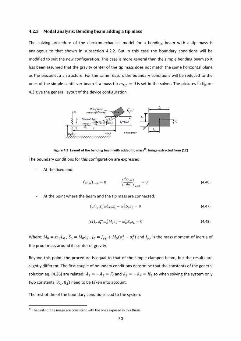
The solving procedure of the electromechanical model for a bending beam with a tip mass is
analogous to that shown in subsection 4.2.2. But in this case the boundary conditions will be
modified to suit the new configuration. This case is more general than the simple bending beam so it
has been assumed that the gravity center of the tip mass does not match the same horizontal plane
as the piezoelectric structure. For the same reason, the boundary conditions will be reduced to the
ones of the simple cantilever beam if a mass tip &0"a = 0is set in the solver. The pictures in figure
4.3 give the general layout of the device configuration.
Figure 4.3 Layout of the bending beam with added tip mass10
. Image extracted from [12]
The boundary conditions for this configuration are expressed:
- At the fixed end:
QAN, = 0QANF , = 0 (4.46)
- At the point where the beam and the tip mass are connected:
GººPNp Gº − PNp 4G = 0 (4.47)
GºººPNp%G − PNp 4Gº = 0 (4.48)
Where: % = &$, 4 = %+,, = +%+,p + +-p and is the mass moment of inertia of
the proof mass around its center of gravity.
Beyond this point, the procedure is equal to that of the simple clamped beam, but the results are
slightly different. The first couple of boundary conditions determine that the constants of the general
solution eq. (4.36) are related: o = −m = oand p = −n = p so when solving the system only
two constants o, p need to be taken into account.
The rest of the of the boundary conditions lead to the system:
10
The units of the image are consistent with the ones exposed in this thesis

31
©oo oppo ppª © o pª = 0 (4.49)
oo = ´sinh MNÜÜÜÜ + sin MNµ + MNm Ý− cosh MN + cos MN + MNp 4Ý ´−sinh MNÜÜÜÜ + sin MNµ (4.50)
op = cosh MN + cos MN + MNm Ý´−sinh MNÜÜÜÜ − sin MNµ + MNp 4Ý − cosh MN + cos MN (4.51)
po = cosh MN + cos MN + MN %ÜÜÜÜ´sinh MNÜÜÜÜ − sin MNµ + MNp 4Ý cosh MN − cos MN (4.52)
pp = ´sinh MNÜÜÜÜ − sin MNµ + MN %ÜÜÜÜcosh MN − cos MN + MNp 4Ý ´sinh MNÜÜÜÜ +sin MNµ (4.53)
The resonance frequencies for each mode are obtained by solving forMNÜÜÜÜsuch that the determinant
equals zero. Successive values of MNÜÜÜÜ correspond again to the beam modes and the natural
frequency of each mode can be determined with PNp = MNÜÜÜÜpÑÀÞcß
Then the general solution is expressed in terms of a single arbitrary constant : QNA = ©coshMNF − cosMNF + opoo sinMNF − sinhMNFª (4.54)
The effective mass%of the structure obtained from the Lagrange equations of motion given in
equation (4.24) is now replaced for the more general expression:
% = « RA0 TQA=
®+ « RA0 T QA=
¯+%´QA$µ0QA$ + 24´QA$µ0QA$
+ ´QAº$µ0QAº$ (4.55)
Lastly, the external work term needs to be re-evaluated to include the inertial loading due to the
proof mass at the beam tip. In eq. (4.30) the forcing vector, was defined to account for the inertial
loading due to a base excitation. It was previously assumed (for simplicity) that the device is of
uniform cross-section in the axial direction. However, the device now consists of two distinct
sections, the uniform beam and uniform proof mass. Both sections contribute to the inertial loading
of the device. The proof mass displacement is calculated in terms of the displacement and rotation of
the tip of the beam. The forcing function definition is extended to account for the proof mass by
including two additional terms in the forcing vector:
32
= &«´QAF µ0F
+ &´QA$µ0 « F à
+ &´QAº$µ0 « F F à
(4.56)
The output values are obtained again using the solution of the governing equations. Expressions from
(4.43) to (4.45) remain exactly the same for the case of the tip mass addition:
Ù ) E½ Ù = 1 Ú1 + HΩpÚj1 − 1 + 2WcHΩpkp + j2Wc + ¥1 + Lp¦HΩ − HΩmkp (4.57)
Ù < E½ Ù = 1|V| HLpΩÚj1 − 1 + 2WcHΩpkp + j2Wc + ¥1 + Lp¦HΩ − HΩmkp (4.58)
Ù ./0 E½ Ù = Po HLpΩpj1 − 1 + 2WcHΩpkp + j2Wc + ¥1 + Lp¦HΩ − HΩmkp (4.59)
Those are the output values taken into account when gathering information to present the results of
the thesis.
33
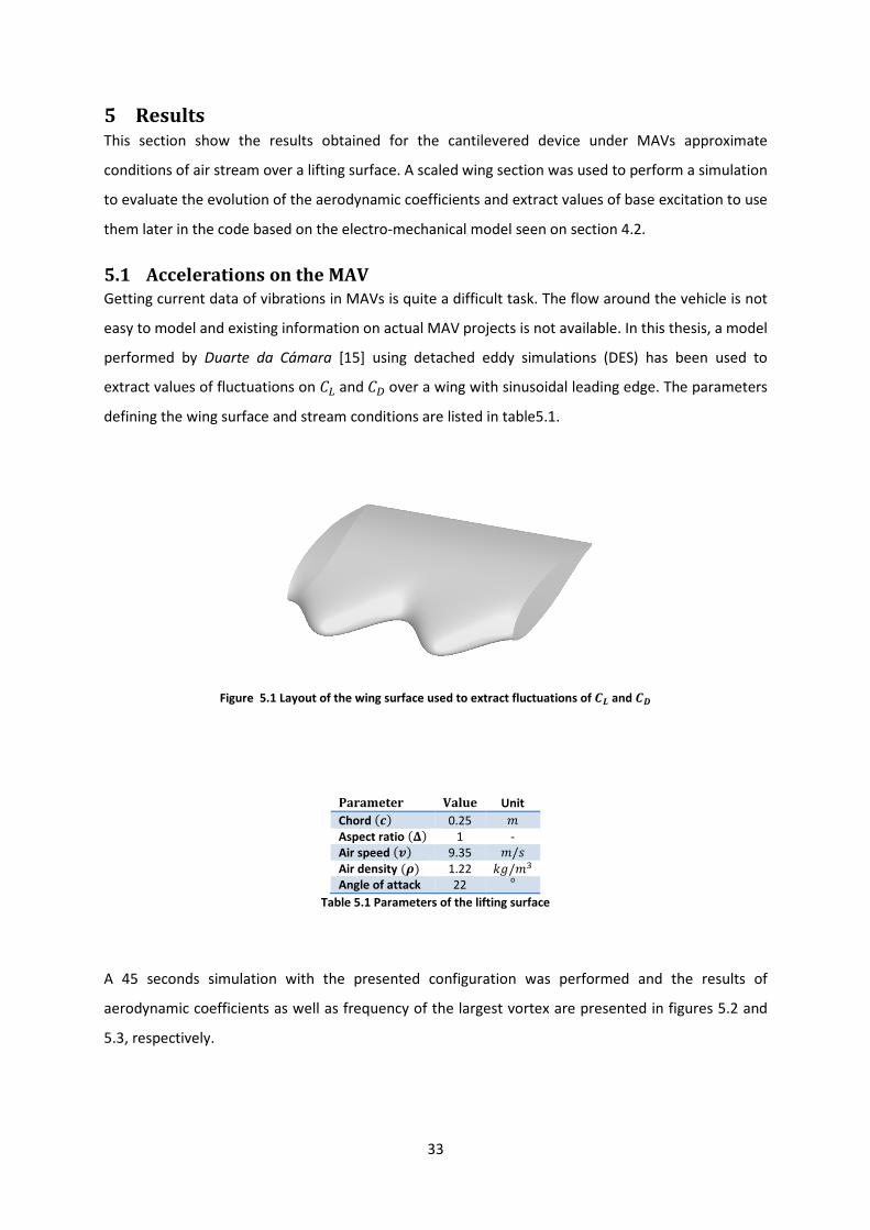
5 Results This section show the results obtained for the cantilevered device under MAVs approximate
conditions of air stream over a lifting surface. A scaled wing section was used to perform a simulation
to evaluate the evolution of the aerodynamic coefficients and extract values of base excitation to use
them later in the code based on the electro-mechanical model seen on section 4.2.
5.1 Accelerations on the MAV
Getting current data of vibrations in MAVs is quite a difficult task. The flow around the vehicle is not
easy to model and existing information on actual MAV projects is not available. In this thesis, a model
performed by Duarte da Cámara [15] using detached eddy simulations (DES) has been used to
extract values of fluctuations on andover a wing with sinusoidal leading edge. The parameters
defining the wing surface and stream conditions are listed in table5.1.
Figure 5.1 Layout of the wing surface used to extract fluctuations of áÉ and áâ
Parameter Value Unit
Chord 0.25 &
Aspect ratio ã 1 -
Air speed ä 9.35 &/]
Air density å 1.22 !e/&m
Angle of attack 22 o
Table 5.1 Parameters of the lifting surface
A 45 seconds simulation with the presented configuration was performed and the results of
aerodynamic coefficients as well as frequency of the largest vortex are presented in figures 5.2 and
5.3, respectively.
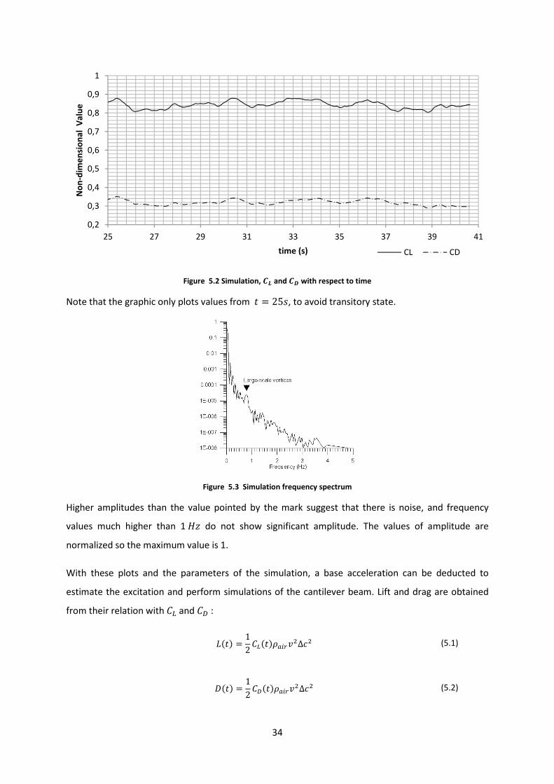
34
Figure 5.2 Simulation, áÉ and áâ with respect to time
Note that the graphic only plots values from8 = 25], to avoid transitory state.
Figure 5.3 Simulation frequency spectrum
Higher amplitudes than the value pointed by the mark suggest that there is noise, and frequency
values much higher than 1hG do not show significant amplitude. The values of amplitude are
normalized so the maximum value is 1.
With these plots and the parameters of the simulation, a base acceleration can be deducted to
estimate the excitation and perform simulations of the cantilever beam. Lift and drag are obtained
from their relation withand: $8 = 1
28T "A<
pΔp (5.1)
8 1
28T "A<
pΔp (5.2)
0,2
0,3
0,4
0,5
0,6
0,7
0,8
0,9
1
25 27 29 31 33 35 37 39 41
No
n-d
ime
nsi
on
al
Va
lue
time (s) CL CD
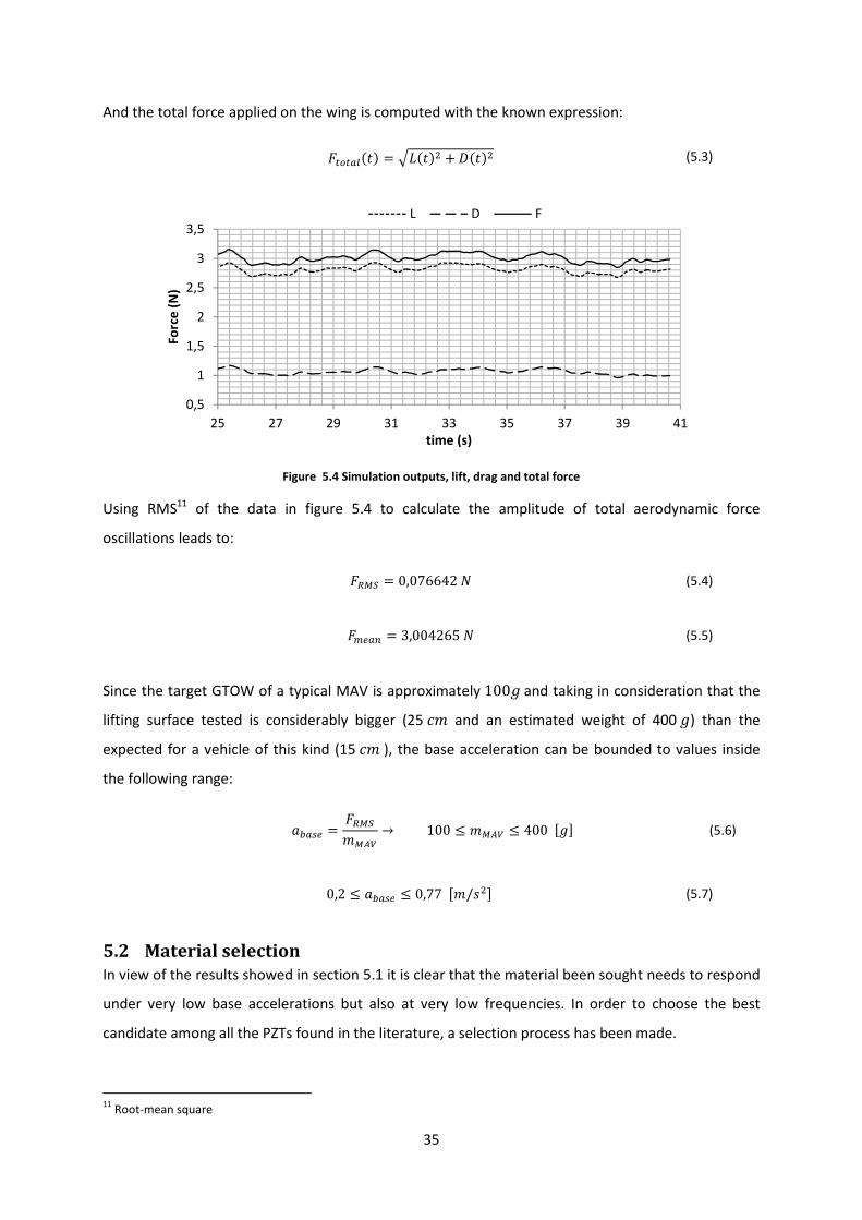
35
And the total force applied on the wing is computed with the known expression:
ç00 8 = Ú$8p + 8p (5.3)
Figure 5.4 Simulation outputs, lift, drag and total force
Using RMS11
of the data in figure 5.4 to calculate the amplitude of total aerodynamic force
oscillations leads to:
ç7èC = 0,076642[ (5.4)
çc 2 = 3,004265[ (5.5)
Since the target GTOW of a typical MAV is approximately100eand taking in consideration that the
lifting surface tested is considerably bigger (25& and an estimated weight of 400e) than the
expected for a vehicle of this kind (15&), the base acceleration can be bounded to values inside
the following range:
= ç7èC&èë
→ 100 ≤ &èë ≤ 400jek (5.6)
0,2 ≤ ≤ 0,77j&/]pk (5.7)
5.2 Material selection
In view of the results showed in section 5.1 it is clear that the material been sought needs to respond
under very low base accelerations but also at very low frequencies. In order to choose the best
candidate among all the PZTs found in the literature, a selection process has been made.
11
Root-mean square
0,5
1
1,5
2
2,5
3
3,5
25 27 29 31 33 35 37 39 41
Fo
rce
(N
)
time (s)
L D F
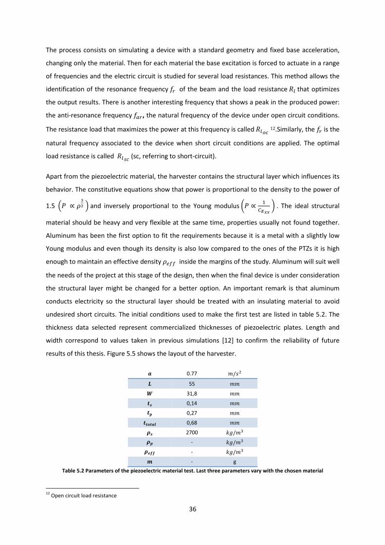
36
The process consists on simulating a device with a standard geometry and fixed base acceleration,
changing only the material. Then for each material the base excitation is forced to actuate in a range
of frequencies and the electric circuit is studied for several load resistances. This method allows the
identification of the resonance frequencyA of the beam and the load resistance that optimizes
the output results. There is another interesting frequency that shows a peak in the produced power:
the anti-resonance frequency A, the natural frequency of the device under open circuit conditions.
The resistance load that maximizes the power at this frequency is called 12.Similarly, the Ais the
natural frequency associated to the device when short circuit conditions are applied. The optimal
load resistance is called (sc, referring to short-circuit).
Apart from the piezoelectric material, the harvester contains the structural layer which influences its
behavior. The constitutive equations show that power is proportional to the density to the power of
1.5_. ∝ TvÔdand inversely proportional to the Young modulus. ∝ oÖîïï. The ideal structural
material should be heavy and very flexible at the same time, properties usually not found together.
Aluminum has been the first option to fit the requirements because it is a metal with a slightly low
Young modulus and even though its density is also low compared to the ones of the PTZs it is high
enough to maintain an effective densityT inside the margins of the study. Aluminum will suit well
the needs of the project at this stage of the design, then when the final device is under consideration
the structural layer might be changed for a better option. An important remark is that aluminum
conducts electricity so the structural layer should be treated with an insulating material to avoid
undesired short circuits. The initial conditions used to make the first test are listed in table 5.2. The
thickness data selected represent commercialized thicknesses of piezoelectric plates. Length and
width correspond to values taken in previous simulations [12] to confirm the reliability of future
results of this thesis. Figure 5.5 shows the layout of the harvester.
ð 0.77 &/]p
É 55 &&
ñ 31,8 &&
| 0,14 &&
0,27 &&
ð~ 0,68 &&
å| 2700 !e/&m
å - !e/&måyy - !e/&mË - g
Table 5.2 Parameters of the piezoelectric material test. Last three parameters vary with the chosen material
12
Open circuit load resistance
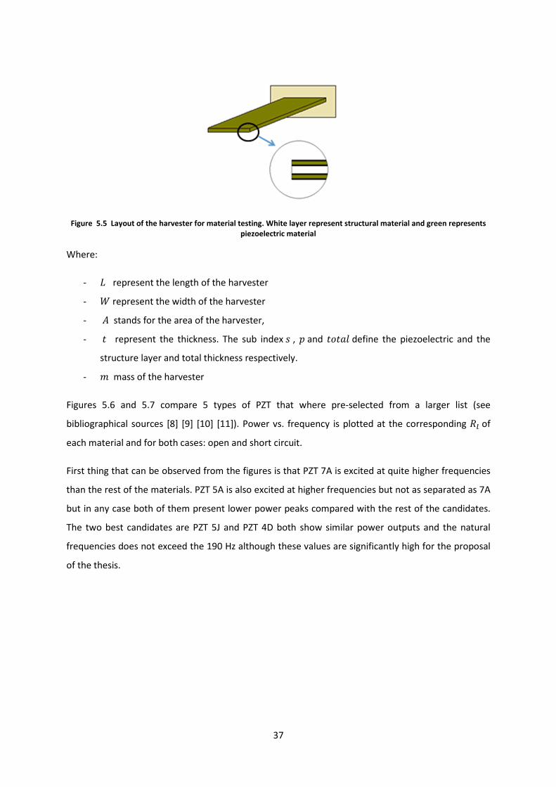
37
Figure 5.5 Layout of the harvester for material testing. White layer represent structural material and green represents
piezoelectric material
Where:
- $ represent the length of the harvester
- ?represent the width of the harvester
- stands for the area of the harvester,
- 8 represent the thickness. The sub index], \and 8+8define the piezoelectric and the
structure layer and total thickness respectively.
- & mass of the harvester
Figures 5.6 and 5.7 compare 5 types of PZT that where pre-selected from a larger list (see
bibliographical sources [8] [9] [10] [11]). Power vs. frequency is plotted at the corresponding of
each material and for both cases: open and short circuit.
First thing that can be observed from the figures is that PZT 7A is excited at quite higher frequencies
than the rest of the materials. PZT 5A is also excited at higher frequencies but not as separated as 7A
but in any case both of them present lower power peaks compared with the rest of the candidates.
The two best candidates are PZT 5J and PZT 4D both show similar power outputs and the natural
frequencies does not exceed the 190 Hz although these values are significantly high for the proposal
of the thesis.

38
Figure 5.6 Power vs. frequency at ~| for each material, short circuit case.
Figure 5.7 Power vs. frequency at ~ for each material, open circuit case.
A final point to be taken into account is the difference between theAand A, the more similar the
frequencies the easier to achieve lower values for both modes altering the geometry like adding a tip
mass. Comparing both materials the conclusion is that PZT 5J is slightly better, as shown in figure 5.8.
0,00E+00
2,00E-07
4,00E-07
6,00E-07
8,00E-07
1,00E-06
1,20E-06
1,40E-06
1,60E-06
1,80E-06
160 180 200 220 240 260
Po
we
r (W
)
Frequency (Hz)
PZT 5J PZT 5H PZT 4D PZT 7A PZT 5A
0,00E+00
2,00E-07
4,00E-07
6,00E-07
8,00E-07
1,00E-06
1,20E-06
1,40E-06
1,60E-06
1,80E-06
160 180 200 220 240 260 280 300
Po
we
r (W
)
Frequency (Hz)
PZT 5J PZT 5H PZT 4D PZT 7A PZT 5A
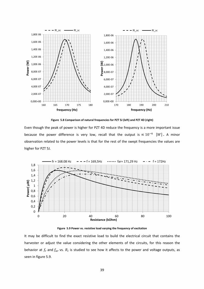
39
Figure 5.8 Comparison of natural frequencies for PZT 5J (left) and PZT 4D (right)
Even though the peak of power is higher for PZT 4D reduce the frequency is a more important issue
because the power difference is very low, recall that the output is∝ 10rò j?k. A minor
observation related to the power levels is that for the rest of the swept frequencies the values are
higher for PZT 5J.
Figure 5.9 Power vs. resistive load varying the frequency of excitation
It may be difficult to find the exact resistive load to build the electrical circuit that contains the
harvester or adjust the value considering the other elements of the circuits, for this reason the
behavior at Aand Avs. is studied to see how it affects to the power and voltage outputs, as
seen in figure 5.9.
0,00E+00
2,00E-07
4,00E-07
6,00E-07
8,00E-07
1,00E-06
1,20E-06
1,40E-06
1,60E-06
1,80E-06
160 165 170 175 180
Po
we
r (W
)
frequency (Hz)
Rl_oc Rl_sc
0,00E+00
2,00E-07
4,00E-07
6,00E-07
8,00E-07
1,00E-06
1,20E-06
1,40E-06
1,60E-06
1,80E-06
170 180 190 200 210P
ow
er
(W)
frequency (Hz)
Rl_oc Rl_sc
0
0,2
0,4
0,6
0,8
1
1,2
1,4
1,6
1,8
0 20 40 60 80 100
Po
we
r( μ
W)
Resistance (kOhm)
fr = 168.08 Hz f = 169,5Hz far= 171,29 Hz f = 172Hz
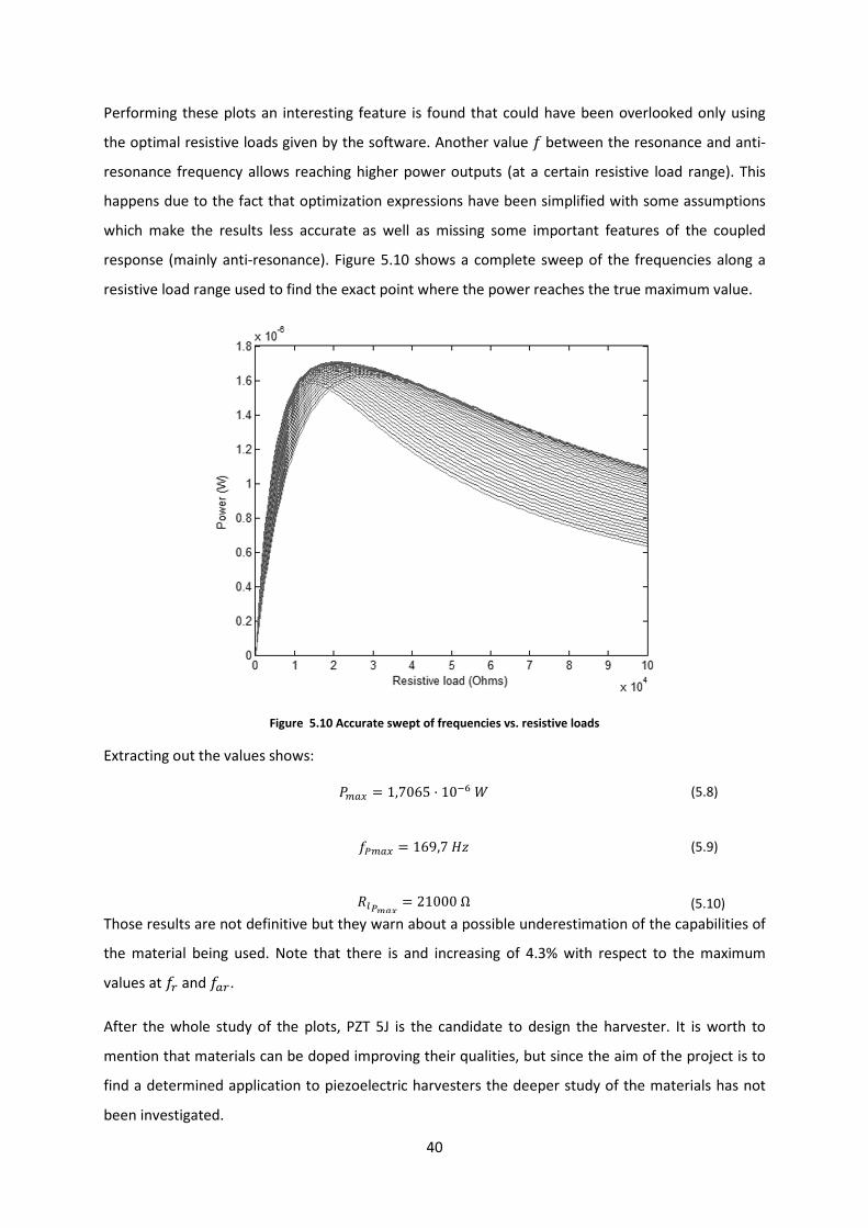
40
Performing these plots an interesting feature is found that could have been overlooked only using
the optimal resistive loads given by the software. Another value between the resonance and anti-
resonance frequency allows reaching higher power outputs (at a certain resistive load range). This
happens due to the fact that optimization expressions have been simplified with some assumptions
which make the results less accurate as well as missing some important features of the coupled
response (mainly anti-resonance). Figure 5.10 shows a complete sweep of the frequencies along a
resistive load range used to find the exact point where the power reaches the true maximum value.
Figure 5.10 Accurate swept of frequencies vs. resistive loads
Extracting out the values shows:
.c , = 1,7065 Ï 10rò? (5.8)
c , 169,7hG (5.9)
ôï 21000Ω (5.10)
Those results are not definitive but they warn about a possible underestimation of the capabilities of
the material being used. Note that there is and increasing of 4.3% with respect to the maximum
values at Aand A.
After the whole study of the plots, PZT 5J is the candidate to design the harvester. It is worth to
mention that materials can be doped improving their qualities, but since the aim of the project is to
find a determined application to piezoelectric harvesters the deeper study of the materials has not
been investigated.
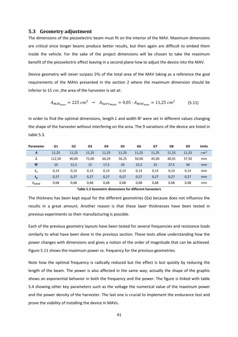
41
5.3 Geometry adjustment
The dimensions of the piezoelectric beam must fit on the interior of the MAV. Maximum dimensions
are critical since longer beams produce better results, but then again are difficult to embed them
inside the vehicle. For the sake of the project dimensions will be chosen to take the maximum
benefit of the piezoelectric effect leaving in a second plane how to adjust the device into the MAV.
Device geometry will never surpass 5% of the total area of the MAV taking as a reference the goal
requirements of the MAVs presented in the section 2 where the maximum dimension should be
inferior to 15& ,the area of the harvester is set at:
èëôï = 225&p → @ ABc , = 0,05 · èëôï = 11,25&p (5.11)
In order to find the optimal dimensions, length$and width?were set in different values changing
the shape of the harvester without interfering on the area. The 9 variations of the device are listed in
table 5.3.
Parameter G1 G2 G3 G4 G5 G6 G7 G8 G9 Units
ö 11,25 11,25 11,25 11,25 11,25 11,25 11,25 11,25 11,25 &p
É 112,50 90,00 75,00 64,29 56,25 50,00 45,00 40,91 37,50 &&
ñ 10 12,5 15 17,5 20 22,5 25 27,5 30 &&
| 0,14 0,14 0,14 0,14 0,14 0,14 0,14 0,14 0,14 &&
0,27 0,27 0,27 0,27 0,27 0,27 0,27 0,27 0,27 &&
ð~ 0,68 0,68 0,68 0,68 0,68 0,68 0,68 0,68 0,68 &&
Table 5.3 Geometric dimensions for different harvesters
The thickness has been kept equal for the different geometries (Gx) because does not influence the
results in a great amount. Another reason is that these layer thicknesses have been tested in
previous experiments so their manufacturing is possible.
Each of the previous geometry layouts have been tested for several frequencies and resistance loads
similarly to what have been done in the previous section. These tests allow understanding how the
power changes with dimensions and gives a notion of the order of magnitude that can be achieved.
Figure 5.11 shows the maximum power vs. frequency for the previous geometries.
Note how the optimal frequency is radically reduced but the effect is lost quickly by reducing the
length of the beam. The power is also affected in the same way; actually the shape of the graphic
shows an exponential behavior in both the frequency and the power. The figure is linked with table
5.4 showing other key parameters such as the voltage the numerical value of the maximum power
and the power density of the harvester. The last one is crucial to implement the endurance test and
prove the viability of installing the device in MAVs.

42
Figure 5.11 Power vs. frequency for nine different devices
Table 5.4 Output results for the different harvesters
Clearly the best configuration is G1 and in general will always be the one with the largest length
value. The center of gravity ÷is moving away from the root so the bending moment gets higher and
increase the stress applied in the piezoelectric layer. For a realistic design the ratio 2`0@ø"10@ or aspect
ratio, cannot be undefinably large for the same reasons why the maximum area is bounded to a 5%
of the total plane area of the MAV.
5
15
25
35
45
55
65
75
85
95
105
10 35 60 85 110 135 160 185 210
Po
we
r (m
icro
W)
Frequency (Hz)
G1 G2 G3 G4 G5
G6 G7 G8 G9
Ëðù zËðù úñ zsû|üý _Ëñþ d
G1 3,80098 101,70 19,9294
G2 2,450077 64,76 12,6898
G3 1,710268 44,97 8,8123
G4 1,249821 33,05 6,4757
G5 0,958238 25,30 4,9569
G6 0,757371 19,99 3,9166
G7 0,61351 16,19 3,1724
G8 0,506854 13,38 2,6220
G9 0,425972 11,24 2,2031

43
G1 length is considerably long but it is taken as the model to add a tip mass and improve even more
the power produced by the harvester. Then it is compared with the endurance studies and if it is
possible, the geometry is adjusted to the optimal shape. Comparing the power density of the
batteries (see section 2.1) and the obtained with the harvesters significant differences can be seen in
the order of magnitude of the output power. This is why the best option is use the geometry (G1)
that provides better results and then find the inferior limits where the harvesters can be included.
Next results show how adding a tip mass to the harvester can improve its performance. The
simulations at this stage where made with the same conditions provided by the lifting surface of
table 5.1 for the geometry G1 and the piezoelectric layers of PZT 5J. Table 5.5 shows the input data.
Initial G1 parameters
ð É ñ | ð~ å| å åyy Ë
0,77 112,5 10 0,14 0,27 0,68 2700 7700 6670 -
Ë/|Ê && && && && && !e/&m !e/&m !e/&m e
Table 5.5 Parameters set for harvester G1 tests
Length$and mass& change depending on the addition of the tip mass dimensions$, &. The
total length of the beam will not increase since it is forced to be$ + $ = 112.5&&. The width will
not be changed as well to preserve the aspect ratio. Table 5.6 show the values obtained for 10
different tip mass dimensions.
É 112,5 111,5 110,5 109,5 108,5 107,5 106,5 105,5 104,5 103,5 102,5 ËË
ñ 10 10 10 10 10 10 10 10 10 10 10 ËË
É 0 1 2 3 4 5 6 7 8 9 10 ËËË 5,1 5,21 5,33 5,44 5,56 5,67 5,79 5,9 6,02 6,13 6,25 y 22,81 22,77 22,73 22,69 22,65 22,61 22,57 22,54 22,5 22,47 22,44
83,74 90,15 96,68 103,33 110,08 116,93 123,86 130,09 137,91 145,01 152,13 úñ 3,80 3,52 3,68 3,83 3,97 4,11 4,24 4,40 4,52 4,67 4,83 5,40E-4 5,58E-04 5,76E-04 5,94E-04 6,11E-04 6,29E-04 6,45E-04 6,61E-04 6,67E-04 6,92E-04 7,07E-04 ËËå 4,9561 5,2083 5,4473 5,689 5,93 6,174 6,4185 6,663 6,908 7,15 7,399
Ëñ/þ
~ 135,89 138,11 140,22 141,97 143,36 144,37 144,99 148,39 148,26 150,98 153,4 þTable 5.6 Geometry and output results with tip mass
For mass tip addition tests, only length is increased instead of adopt other solutions like change the
thickness for the reason that MAV thickness (mainly airfoil thickness) is limited and increasing this
value in the harvester could lead to be unable to place the device inside the structure.

44
The output values are presented in figures 5.12 to 5.14 as well, so that the tendency of the results is
easier to identify.
Figure 5.12 Frequency vs. tip length
Figure 5.13 Power vs. tip length
Figure 5.14 Resistive Load vs. tip length
20
21
22
23
24
25
26
0 1 2 3 4 5 6 7 8 9 10
Fre
qu
en
cy (
Hz)
Tip length L0 (mm)
60
70
80
90
100
110
120
130
140
150
160
0 1 2 3 4 5 6 7 8 9 10
Po
we
r (µ
W)
Tip length L0 (mm)
130000
135000
140000
145000
150000
155000
0 1 2 3 4 5 6 7 8 9 10
Loa
d r
esi
sta
nce
(O
hm
s)
Tip length L0 (mm)
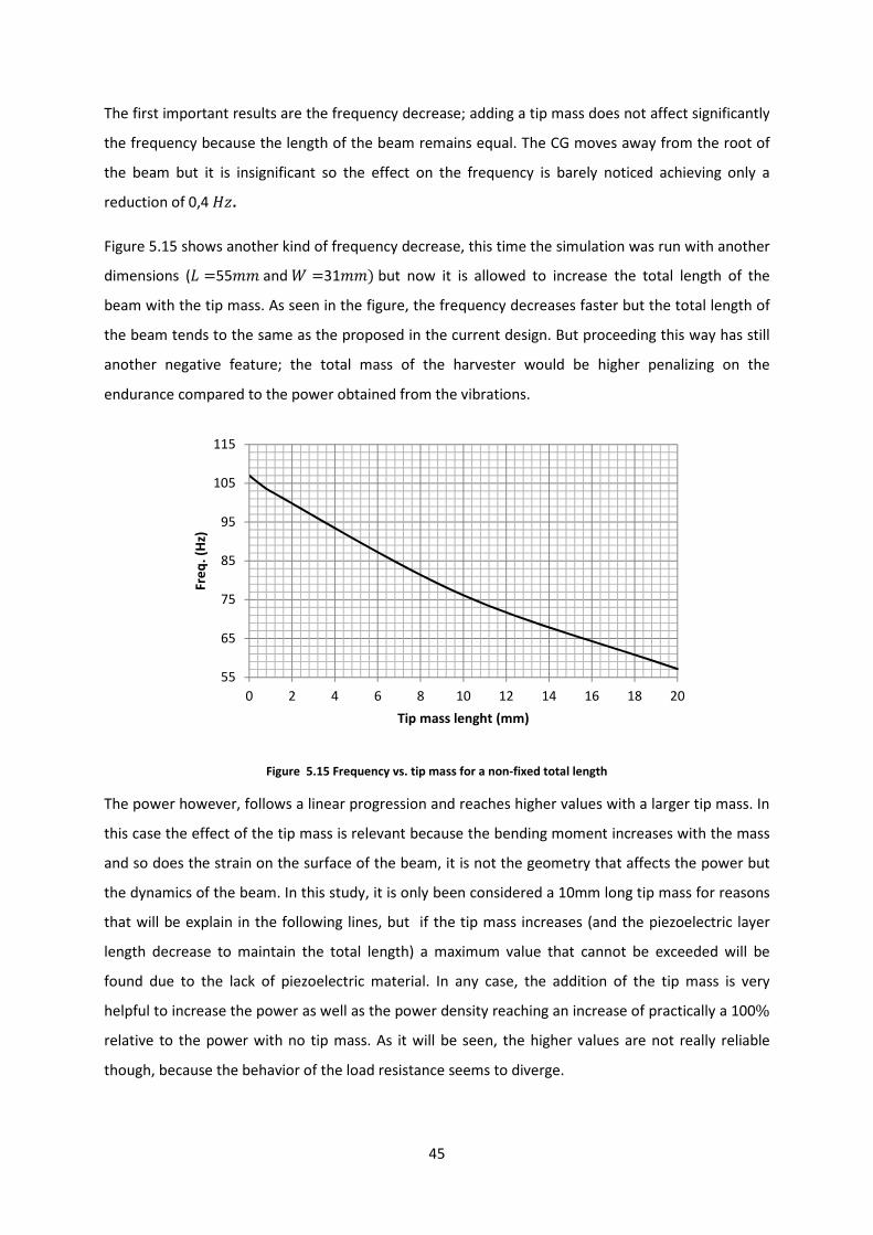
45
The first important results are the frequency decrease; adding a tip mass does not affect significantly
the frequency because the length of the beam remains equal. The CG moves away from the root of
the beam but it is insignificant so the effect on the frequency is barely noticed achieving only a
reduction of 0,4 hG.
Figure 5.15 shows another kind of frequency decrease, this time the simulation was run with another
dimensions ($ =55&&and? =31&&but now it is allowed to increase the total length of the
beam with the tip mass. As seen in the figure, the frequency decreases faster but the total length of
the beam tends to the same as the proposed in the current design. But proceeding this way has still
another negative feature; the total mass of the harvester would be higher penalizing on the
endurance compared to the power obtained from the vibrations.
Figure 5.15 Frequency vs. tip mass for a non-fixed total length
The power however, follows a linear progression and reaches higher values with a larger tip mass. In
this case the effect of the tip mass is relevant because the bending moment increases with the mass
and so does the strain on the surface of the beam, it is not the geometry that affects the power but
the dynamics of the beam. In this study, it is only been considered a 10mm long tip mass for reasons
that will be explain in the following lines, but if the tip mass increases (and the piezoelectric layer
length decrease to maintain the total length) a maximum value that cannot be exceeded will be
found due to the lack of piezoelectric material. In any case, the addition of the tip mass is very
helpful to increase the power as well as the power density reaching an increase of practically a 100%
relative to the power with no tip mass. As it will be seen, the higher values are not really reliable
though, because the behavior of the load resistance seems to diverge.
55
65
75
85
95
105
115
0 2 4 6 8 10 12 14 16 18 20
Fre
q.
(Hz)
Tip mass lenght (mm)
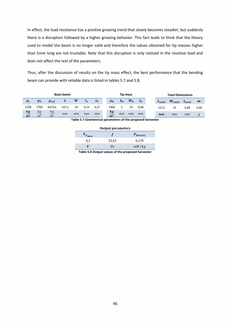
46
In effect, the load resistance has a positive growing trend that slowly becomes steadier, but suddenly
there is a disruption followed by a higher growing behavior. This fact leads to think that the theory
used to model the beam is no longer valid and therefore the values obtained for tip masses higher
than 5mm long are not trustable. Note that this disruption is only noticed in the resistive load and
does not affect the rest of the parameters.
Thus, after the discussion of results on the tip mass effect, the best performance that the bending
beam can provide with reliable data is listed in tables 5.7 and 5.8.
Basic beam å| å åyy É ñ |
2700 7700 6670,6 107,5 10 0,14 0,27
þËt
!e&m
!e&m && && && &&
Tip mass
å É ñ 7400 5 10 0,68
þËt && && &&
Total Dimensions
Éð~ ñð~ ð~ Ë 112,5 10 0,68 5,68
ËË && && e
Table 5.7 Geometrical parameters of the proposed harvester
Output parameters
Ëðù y sû|üý
4,1 22,61 6,174
hG &?/!e
Table 5.8 Output values of the proposed harvester
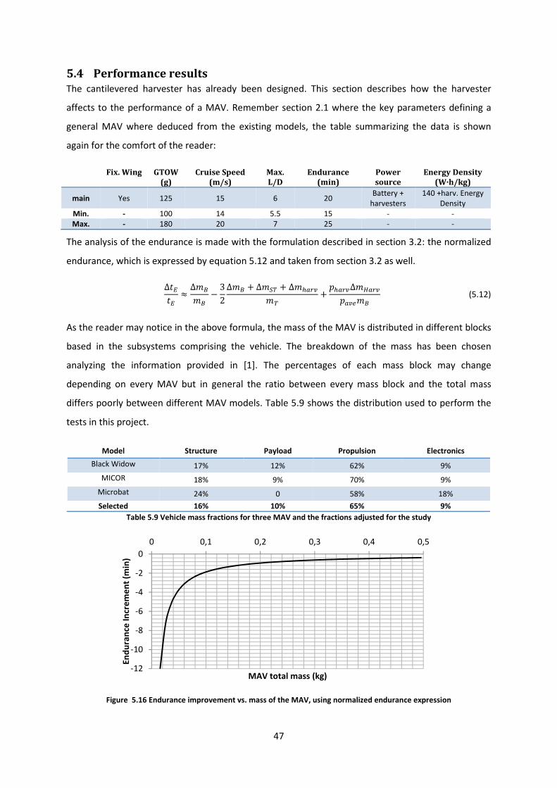
47
5.4 Performance results
The cantilevered harvester has already been designed. This section describes how the harvester
affects to the performance of a MAV. Remember section 2.1 where the key parameters defining a
general MAV where deduced from the existing models, the table summarizing the data is shown
again for the comfort of the reader:
Fix. Wing GTOW
(g)
Cruise Speed
(m/s)
Max.
L/D
Endurance
(min)
Power
source
Energy Density
(W·h/kg)
main Yes 125 15 6 20 Battery +
harvesters
140 +harv. Energy
Density
Min. - 100 14 5.5 15 - -
Max. - 180 20 7 25 - -
The analysis of the endurance is made with the formulation described in section 3.2: the normalized
endurance, which is expressed by equation 5.12 and taken from section 3.2 as well.
Δ8989 ≈ Δ&& − 32Δ& + Δ&CD + Δ&@ AB&D + \@ ABΔ& AB\ B& (5.12)
As the reader may notice in the above formula, the mass of the MAV is distributed in different blocks
based in the subsystems comprising the vehicle. The breakdown of the mass has been chosen
analyzing the information provided in [1]. The percentages of each mass block may change
depending on every MAV but in general the ratio between every mass block and the total mass
differs poorly between different MAV models. Table 5.9 shows the distribution used to perform the
tests in this project.
Model Structure Payload Propulsion Electronics
Black Widow 17% 12% 62% 9%
MICOR 18% 9% 70% 9%
Microbat 24% 0 58% 18%
Selected 16% 10% 65% 9%
Table 5.9 Vehicle mass fractions for three MAV and the fractions adjusted for the study
Figure 5.16 Endurance improvement vs. mass of the MAV, using normalized endurance expression
-12
-10
-8
-6
-4
-2
0
0 0,1 0,2 0,3 0,4 0,5
En
du
ran
ce I
ncr
em
en
t (m
in)
MAV total mass (kg)

48
Figure 5.16 shows a clear result. Adding the piezoelectric harvester only leads to losing minutes of
flight. If the mass of the MAV is increased (keeping the mass of the harvester), then the flight
endurance is not so impaired. The maximum loss would be 22,2 seconds but it would be impossible
to get a positive result. The reason of the endurance loss is caused by the small specific power
(?/!e) that the harvester is able to provide. The accelerations acting on the root of the beam are
very weak making impossible to force the beam getting stronger stress values; therefore the specific
power does not increase enough. But the specific power is not the only problem, another important
feature is the mass added by the harvester. In the case showed in figure 5.16, the harvester is added
as an extra mass to the MAV, structure, payload, electronics and propulsion remains intact, so
equation (5.12) is reduced to the following expression, and is then used to perform the graphic of
figure 5.16.
Δ8989 ≈ −32
Δ&@ AB&D
+ \@ ABΔ& AB\ B&
(5.13)
Δ& = Δ&CD = Δ& = 0 (5.14)
The contribution of the first term on the right side of equation (5.13) is very high compared to the
positive term involving the specific power. So an alternative solution must be designed in order to
reduce or ban the effect of the term:
−32Δ&@ AB&D
(5.15)
Or in the general form:
−32Δ& + Δ&CD + Δ&@ AB
&D (5.16)
In effect, there is a solution that can cancel the negative term. The idea is to implement the harvester
with a double function, be the actual harvester and be part of the structure of the MAV as well. This
can be pictured as a fixed wing but instead of being completely made of foam, or composite material
the piezoelectric harvester would be a structural beam in the skeleton of the MAV substituting part
of the original material.
If this was the case, thenΔ&@ AB = −Δ&CD. Since the batteries will not change their massΔ& =0. Leading to:

49
−32Δ& + Δ&CD + Δ&@ AB&D = 0 (5.17)
The endurance now is expressed by the following equation:
Δ8989 ≈ \@ ABΔ& AB
\ B& (5.18)
This expression can only be positive and ensures an increase of the flight time. Taking into account
that the effect of this term is considerably smaller than the negative term of equation (5.15), the
prediction of the results leads to think that the positive contribution may not be significantly high
and it has no impact on the endurance of the MAV.
Figure 5.17 Increment of the endurance vs. the total mass of the MAV
After the graphic representation (Figure 5.15), the increment of the endurance is completely
unnoticed which to the same conclusion: With the current technology, the specific power is too small
to provide extra flight time.
5.5 Evaluation of the solution
The cantilevered harvester seems to be a solution applied to an incorrect range of dimensions. It
would be a suitable solution if the external conditions affecting the MAV, specifically the base
accelerations, were higher. The maximum specific power that a piezoelectric can provide may be
enough to power another kind of vehicle that require less energy, then again, the dimensions of the
0,00005
0,000055
0,00006
6,5E-05
7E-05
7,5E-05
8E-05
0 0,1 0,2 0,3 0,4 0,5
En
du
ran
ce I
ncr
em
en
t (m
in)
MAV mass (kg)

50
harvester would be forced to reduce making difficult to confirm or deny a positive solution in terms
of power production.
In terms of frequency excitation, the results are not positive either. The target of 0,8 Hz is too small
for the restrictions imposed by the MAV, making possible only a reduction of the frequency until 20
Hz, a frequency only achievable forcing the harvester to be as large as possible. It looks like the
piezoelectric technology has a better application for medium and high frequency conditions if the
configuration implemented is a cantilever beam.
To sum up, an alternative solution for the implementation of a cantilever harvester in an MAV should
suit the two main requirements discussed in the previous paragraphs. It must be subjected to a
medium/high frequency excitation environment and must be located in a place where it could take
profit of high base accelerations.
If placing the harvester inside the MAV is not a solution, then the first option that comes to mind is
place it outside the vehicle as an aerodynamic appendix. The direct contact with the air stream may
induce higher stress in the harvester improving the specific power. A resizing would be necessary,
not only to optimize the dimensions, but mainly to avoid aerodynamic problems on the surface of
the MAV, namely a dramatic increase of the drag that could vanish a possible benefit from the
harvester electric power supply.
A complement for any other useful solution for the implementation of this kind of harvesters on
MAVs is the design of clusters. Clusters are a connection of various harvesters. If the specific power
produced is enough but the output power needs to be higher, the connection in series or parallel of
various devices would be the easiest solution instead of designing a larger and more complex
harvester. In case of use the clusters as a way to increase the endurance it will end failing due to the
mass addition in front of the power supply. That is why the target using cluster would not be increase
endurance but to be used as a way to power distributed microelectronics in MAVs.
5.6 Validation
After the deep study of the configuration and due to the rather negative results, the validation of the
work done is more than a merely prove of the reliability of this thesis but a way to find out if there
were still a possibility to implement this configuration in such a way that permits achieving positive
results. The literature is plenty of electromechanical models and cantilever harvester papers (see
bibliography) and in this section it will be commented some of them comparing its results with the
ones obtained in the project.

51
Since the code used to develop this study was incomplete, a first validation was made to check
whether if the completion of the code was successful or not. To do so, a replica of the simulation
done by du Toit [12]about a PZT 5A cantilever harvester was made leading to the same values, a fact
that confirmed the successful completion of the software. Too see the comparison between the
values of the original study with the ones of the thesis please refer to annex B, where power, voltage
and tip displacement graphs are plotted.
The next part of the validation refers to the results obtained under the restrictions imposed in this
project. This would be a base acceleration smaller than 1 &/]p with harvesters made of PZT type
piezoelectric layers. As it has been already said, the literature is extensive on this topic but there is
no information about the implementation on MAVs. That makes difficult to find simulation papers
with similar conditions. However, it is possible to check different parameters separately due to the
relation of the geometrical dimensions of the beam with the resonance frequency. Thus in Wang et
al [16] a simulation with a cantilever harvester, whose parameters are reproduced in Table 5.10, is
carried out.
Table 5.10 Parameters for a cantilever harvester simulation in Wang et al [16]
The dimensions of this harvester are similar to the ones shown in section 5.3. Table 5.3 and Figure
5.11 show that G4 ($=64,29&&, ?=17,5&&, 8=0,27&&) and G5 ($=56,25&&, ?=20.0&&, 8=0,27&&) harvesters’ dimensions are similar and the resonance frequency lay in the same range
close to 80hG.
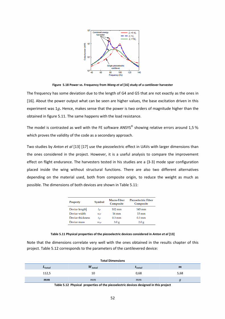
52
Figure 5.18 Power vs. Frequency from Wang et al [16] study of a cantilever harvester
The frequency has some deviation due to the length of G4 and G5 that are not exactly as the ones in
[16]. About the power output what can be seen are higher values, the base excitation driven in this
experiment was 1e. Hence, makes sense that the power is two orders of magnitude higher than the
obtained in figure 5.11. The same happens with the load resistance.
The model is contrasted as well with the FE software ANSYS©
showing relative errors around 1,5%
which proves the validity of the code as a secondary approach.
Two studies by Anton et al [13] [17] use the piezoelectric effect in UAVs with larger dimensions than
the ones considered in the project. However, it is a useful analysis to compare the improvement
effect on flight endurance. The harvesters tested in his studies are a 3-3 mode spar configuration
placed inside the wing without structural functions. There are also two different alternatives
depending on the material used, both from composite origin, to reduce the weight as much as
possible. The dimensions of both devices are shown in Table 5.11:
Table 5.11 Physical properties of the piezoelectric devices considered in Anton et al [13]
Note that the dimensions correlate very well with the ones obtained in the results chapter of this
project. Table 5.12 corresponds to the parameters of the cantilevered device:
Table 5.12 Physical properties of the piezoelectric devices designed in this project
Total Dimensions
Éð~ ñð~ ð~ Ë112,5 10 0,68 5,68
ËË && && e
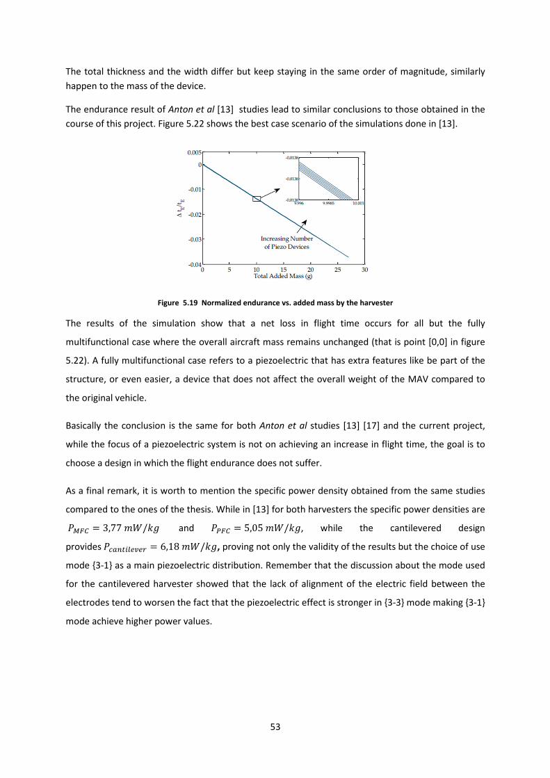
53
The total thickness and the width differ but keep staying in the same order of magnitude, similarly
happen to the mass of the device.
The endurance result of Anton et al [13] studies lead to similar conclusions to those obtained in the
course of this project. Figure 5.22 shows the best case scenario of the simulations done in [13].
Figure 5.19 Normalized endurance vs. added mass by the harvester
The results of the simulation show that a net loss in flight time occurs for all but the fully
multifunctional case where the overall aircraft mass remains unchanged (that is point [0,0] in figure
5.22). A fully multifunctional case refers to a piezoelectric that has extra features like be part of the
structure, or even easier, a device that does not affect the overall weight of the MAV compared to
the original vehicle.
Basically the conclusion is the same for both Anton et al studies [13] [17] and the current project,
while the focus of a piezoelectric system is not on achieving an increase in flight time, the goal is to
choose a design in which the flight endurance does not suffer.
As a final remark, it is worth to mention the specific power density obtained from the same studies
compared to the ones of the thesis. While in [13] for both harvesters the specific power densities are .èÖ = 3,77&?/!e and .Ö = 5,05&?/!e, while the cantilevered design
provides. 20"BA = 6,18&?/!e, proving not only the validity of the results but the choice of use
mode 3-1 as a main piezoelectric distribution. Remember that the discussion about the mode used
for the cantilevered harvester showed that the lack of alignment of the electric field between the
electrodes tend to worsen the fact that the piezoelectric effect is stronger in 3-3 mode making 3-1
mode achieve higher power values.
54
6 Theoretical approach on an external device configuration.
In view of the results shown in the previous section, it seems necessary another point of view of the
problem, which is finding a different placement for the piezo-harvester. The goal is to increment the
acceleration applied on the harvester’s body, however this means placing the device outside the
MAV so the flow can interact along with the base acceleration (produced by the MAV structure),
hence providing an extra force of aerodynamic origin.
This approach raised some difficulties that have led this project to avoid any simulated or
experimental study. That is why this chapter aims to show the reasons of the taken decision based on
the results that have been already exposed in the previous chapter as well as studies of external
bibliographic sources and the limitations for implementing a code based on the inner device
approach.
6.1 Initial planned solution
The first solution considered to analyze the external device was to improve the code used in section
5, adding the aerodynamic force to the base excitation and hence obtain results of the combined
accelerations. In order to carry on with the aerodynamic excitation, the main point was to use results
of previous studies on MAVs to perform the tests; in particular the thesis by Camara [15] was the
first option because of the study of the vorticial flow in sinusoidal leading edge wings. The same
source was used to evaluate the base acceleration in the previous chapters, so at first glance it is a
good choice.
The main problem that faced this solution was the linkage between the code already built and the
output of the flow studies, specifically how to add an extra excitation over the device that acts as a
base acceleration. Let us not forget that the code used in the thesis is based in a cantilever beam
configuration, thus the addition of extra excitation must be consequent with the boundary
conditions of the problem. That is really a big issue because a cantilevered beam subjected to a free
stream activates not only the bending modes but also the torsional modes, changing in great
measure the physics of the problem. Aside of the mechanical behavior, there is the coupling effect
with the piezoelectric material and then adding a time depending turbulent flow would complicate in
highly the study of the external device approach.
As a result, all these complications lead to build a specific code only for the study of this particular
case. It is not an impossible task; however the time and effort needed to create a reliable code are
out of the range for this thesis, although it would be possible if there is a continuation (in future
studies) focused in this approach of the MAVs piezoelectric harvesters.
55
Needless to say that before to proceed with such a work, the feasibility of the solution should be
carried out in order to prevent undesired or unusable results. The last section of this chapter is
dedicated to this topic and although there are not really high expectations of the feasibility of outer
piezoelectric devices there is not a solid answer denying the study of this issue. The discussion will be
explained after showing some other studies related to immersing a piezoelectric harvester in an air
flow.
6.2 Other studies
After the difficulties faced in the proposed solution to approach the outer device configuration, the
use of published studies in the literature was an incentive to continue investigating how to solve the
problem. Here are included the considered works, their approach and the problems that were faced
when considering its application.
6.2.1 Double-Lattice method for aero-elastic vibrations modeling
The idea is developed by De Marqui and Vieira [18] and the main point of the paper is to combine
the doublet-Lattice method with the electro-mechanical coupled equations (already developed in
section 4.2) to obtain the output power produced by both base and aerodynamic excitations. The
addition of the aero-elastic behavior is made by a linearized formulation for the oscillatory, inviscid,
subsonic lifting surface theory which relates the normal velocity over a surface with the aerodynamic
loads caused by the pressure distribution.
The formulation is derived from flow equation for unsteady potential flow. The potential of a doublet is
the solution used to solve the Euler equations and hence obtain the unsteady aero-elastic behavior
as well as the resultant differential pressure across the surface of a wing or a lifting surface in this
case
The discretization of the thin lifting surface includes a doublet in each element. Then, solving the
equation for each element leads to obtain a matrix of influence that will be added to the electro-
mechanical model.
This approach was a good solution for the study of the outer device configuration. Nevertheless, the
problems mentioned at the beginning of the chapter still remain. Those are the addition of torsion
modes besides the bending ones and the necessity of build a new code to work with. This paper was
used as a validation of the primary idea exposed in the section before but it was an aware (too), of
the complications facing the development of the study which ended up with the decision of avoid
any study because of possible unreliable results, which in turn could affect negatively on the project.

56
6.2.2 T-shaped cantilevers subjected to an air stream
The paper described by Kwon [19] is an experimental description of a T-Shaped structure subjected
to an air stream. The idea is to reach the flutter frequencies of the beam to obtain a sustained and
slightly constant power output. The following figure is a scheme of the layout:
Figure 6.1 Layout of the T-shaped cantilever beam from Kwon [19]
The beam is then introduced in the wind tunnel where the wind velocity can be adjusted, the
piezoelectric electrodes are connected to a multimeter and the displacement is captured by a CCD
camera and using image processing techniques.
Although the layout is considerably different from the one proposed originally in this thesis, the
advantage is that it could have been used for validation of possible studies. There are empirical
correlations that complete the experimental data which may be used for our cause.
Again, the possibility to investigate through this line was questioned because of the dimensions of
the piezoelectric layers, and the whole device in general. The external appendices that an MAV can
afford to add outside of the fuselage must be very small in order to avoid drag problem, loss of lift or
even loss of endurance by weight addition. Thus, the possibility of using the empirical correlation for
smaller devices and also that do not match with the geometry of the proposed paper is highly
questionable.
6.3 Feasibility of the configuration
In view of the previous issues to carry on with the study of an external device on MAVs, a natural
question came out, motivated largely by the results obtained in the study of the embedded
piezoelectric approach. That is, to question the feasibility of using piezoelectric in MAVs regardless of
the position inside or outside the structure of the vehicle. It is clear, that an internal device is not
intended to be used as a complementary source of propulsion and even try to use it as a power
source for installing extra electronics might be worthless because of the endurance loss. However,
for external devices, it happens to be unclear whether if increase the capabilities of the MAV (in

57
terms of information that is able to gather) is a plausible solution or not. The results of the sources
described above indicate that similarly to the internal approach the devices are unable to provide
more than 1 &?. The results shown in Kwon [19] for a three piezoelectric layers device with
dimensions13$ = 100&&, = 60&&,h = 30&& subjected to a wind speed of 4,6&/] and a
tip mass of 15,5e are presented in figures 6.2 and 6.3.
Figure 6.2 Output performance for a T-shape device with 6Hz vibrations from Kwon [19]
The power increases until 4&? if the speed is raised up until 15 &/] which is the target speed of
the MAV’s point of design of this thesis (see figure 6.3). This is a slightly better result than the one
obtained for the internal device. Still the geometry proposed in this paper presents impediments to
apply something similar to the fuselage of an MAV. Starting from the mass proof, the weight is much
higher than the affordable both for the endurance and the aerodynamics. The size of the complete
device is also out of the boundaries and the outputs certainly will not be enough for an increment of
the flight time.
Figure 6.3 Power vs. wind speed comparison from Kwong [19]
13
The dimensions are in accordance to the nomenclature shown in figure 6.1

58
Nonetheless, the doubt of the usefulness remains if these devices can be installed in larger MAVs, or
safer say small UAVs, where the mass of the harvester is negligible in front of the mass of the vehicle,
making it a better solution for the installation of extra features in the MAV.
Then external devices, at first glance, seem better sources of power than the internal device
configuration, but the lack of information regarding the vibrations of aero-elastic effects makes it
difficult to dismiss or approve this option. Take into account that the conditions where these devices
have been tested are different than the ones occurring around a MAV/UAV fuselage. After all the
discussion, the most reasonable plan should be a proper study of the flow around an MAV model
capturing the acceleration in critical points of the structure and then discern whether it is worthwhile
to continue an investigation on this line.
59
7 Conclusions and future work
The studies performed during this thesis were focused on the assessment of electric power that a
cantilever harvester can provide placing the device inside a fixed-wing MAV structure. The objective
was using this energy as a primary recharging method to extend the endurance of such vehicles
The results show piezoelectric materials cannot be a primary source for recharging the batteries of
the propulsion system. The study of the excitations acting over the structure of an MAV (represented
as a sinusoidal leading edge flying wing) revealed low accelerations acting at proximately 1Hz
frequencies. Those restrictions were considered when designing the cantilevered harvester leading
to power outputs of a few &? at ~20 Hz frequencies. Both tasks (reaching the goal excitation
frequency and provide enough power to feed the batteries) were infructuous due to size limitation of
the harvester and lack of higher excitations. The link between the geometrical shape of the beam
and the natural frequency showed the major necessity of high aspect ratio dimensions but the size of
the MAV reduce the length and width to a maximum amount that cannot be exceeded. Thus the area
of the harvester is limited (as well as the piezoelectric material) and, with the already mentioned
excitations, it is not possible to reach the desired output requirements.
An external harvester configuration was also considered but research on literature showed similar
results for devices placed in free streams with similar velocities to MAVs. This fact and the complexity
to build a code to simulate the behavior of a beam subjected to the air flow discouraged a deeper
study of this approach.
The validation of the code used for the simulations along with comparison of cantilever harvester
studies ensures the solid results of the thesis. Even in larger scale vehicles, like small UAVs, studies
show piezoelectricity is suitable only as secondary power sources, such as feeding electronics of the
aerial vehicle. In order to not lose endurance, the devices must have a multifunctional purpose, so
that the overall weigh is not increased.
At this point the reader may find discouraging future studies on piezoelectricity as an application for
MAVs but certainly what this thesis has reached is to point the strong relation between the behavior
of the surrounding environment over the MAV with the harvester performance, which helps to find
new situations where this technology has better chances to fulfill positive results.
As an example, think about carrying a larger payload without penalties on the endurance. This
branch is currently under study not only for MAVs but for other vehicles and systems with
multipurpose tasks.

60
Another possibility is to study the availability of using the piezoelectric effect in the propulsion
system of flapping wing MAVs. This vehicle configuration needs a large amount of continuous power
but the batteries cannot typically afford more than 2 minutes of flight time. Taking advantage from
the flapping wings as a source of excitation for piezoelectric layers may extend the endurance.
And lastly, the reverse piezoelectric effect is also a challenge. Using a voltage input to make
piezoelectric wings flap would reduce the necessity of mechanical parts in the vehicle, reducing
weight that can be used for extra features.
61
Bibliography
[1] F. Bohorquez y D. J. Pines, Challenges Facing Future Micro-Air-Vehicle Development, vol. 43,
Journal of Aircraft, April 2006.
[2] A. Epstein, S. Senturia, O. Al-Midani, G. Anathasuresh, A. Ayon, K. Breuer, K.-S. Chen, F. Ehrich, E.
Esteve, L. Frechette, G. Gauba, R. Ghodssi, C. Groshenry, S. Jacobson, J. Kerrebrock, J. Lang, C.-C.
Lin, A. London, J. Lopata, A. Mehra, J. Mur, S. Nagle, D. Or, E. Piekos, M. Schmidt, G. Shirley, S.
Spearing, C. Tan, Y.-S. Tzeng y I. Waitz, «Micro-Heat Engines, Gas Turbines, and Rocket Engines,
The MIT Micro-engine Project,» Massachusetts Institute of Technology, Cambridge, 1997.
[3] W. J. Wu y B. S. Lee, Piezoelectric MEMS Power Generators for Vibration Energy Harvesting,
Taipei: Department of Engineering Science and Ocean Engineering, pp. 135-157.
[4] D. Guyomar, A. Badel, E. Lefeuvre y C. Richard, Toward energy harvesting using active materials
and conversion improvement by nonlinear processing, vol. 52, IEEE Transactions on, 2005, pp.
584-595.
[5] E.Lefeuvre, A.Badel, L. L. A. Benayad, C.Richard y D.Guyomar, A Comparison Between several
Approaches of Piezoelectric Harvesting, vol. 128, Journal De Physique IV, 2005, pp. 177-186.
[6] A.Badel, D. Guyomar, E.Lefeuvre y C.Richard, Efficiency enhacement of a piezoelectric energy
harvesting device in pulsed operation by synchronous charge inversion, vol. 16, Journal of
intelligent material systems and structures, 2005, pp. 889-901.
[7] Y. Jeon, R. Sood, J.H.Jeong y S. Kim, MEMS power generator with transverse mode thin film PZT,
Sensors and Actuators -A: Physical, n16, pp. 2253-2264, 2005.
[8] «Piezo Technologies,» 2014. [On line]. Available:
http://www.piezotechnologies.com/Ceramics/Datasheets.aspx. [Last acces: 16 July 2014].
[9] PI Ceramic GmbH, PI Ceramic, 2014. [On line]. Available:
http://piceramic.com/products/piezoelectric-materials.html. [Last acces: 16 July 2014].
[10] SG3 Knowledge Network OG , PiezoMat, 2014. [On line]. Available: http://piezomat.org/. [Last
acces: 2014 July 17].
[11] Arkema Group, Piezotech, 2014. [On line]. Available:
http://www.piezotech.fr/image/documents/22-31-32-33-piezotech-piezoelectric-films-
leaflet.pdf. [Last acces: 20 July 2014].
[12] M. Du Toit, Modeling and design of a MEMS Piezoelectric Vibration Energy Harvester, MIT, 2005.
[13] S. R. Anton, Multifunctional Piezoelectric Energy Harvesting Concepts, Blacksburg, 2011.

62
[14] J. Wang, Y.-K. Yong y T. Imai, Finite Element Analysis of the Piezolectric Vibration of Quartz Plate
Ressonators with Higher-order Plate Theory, Orlando, FL: IEEE International Frequency Control
Symposium, 1997, p. 9.
[15] J. F. D. d. Camara, Controlo Passivo da Perda em Micro-Veículos Aéreos Usando Bordos de
Ataque Sinusoidais, Master thesis in Aerospace Engineering, Universidade deLisboa, 2012.
[16] h.-y. Wang, X.-b. Shan y T. Xie, An energy harvester combining a piezoelectric cantilever and a
single degree of freedom elastic system, Journal of Zhejiang University-ScienceA (Appl Phys &
Eng), vol. 13, n 7, pp. 526-537, 2012.
[17] S. R. Anton, A.Erturk y D. Inman, An Investigation on Piezoelectric Composite Spars forEnergy
Harvesting in Unmanned Aerial Vehicles, Blacksburg, VA.
[18] C. D. M. Jr. y W. G.R.Vieira, Modeling and Analysis of Piezoelectric Energy Harvesting From
Aeroelastic Vibrations Using the Doublet-Lattice Method, Journal of Vibration and Acoustics, vol.
133, pp. 1-9, February 2011.
[19] S.-D. Kwon, A T-Shaped piezoelectric cantilever for fluid energy harvesting, Applied Physics
Letters, nº 97, p. 3, 2010.
[20] N. Hagood, W.Chung y V. Flotow, Modelling of piezoelectric actuator dymnamics for active
structural control, Journal of intelligent Material Systems and Structures: Vol.1, n 3, pp. 327 -
354, 1990.
[21] J. P. Thomas, M. A. Qidwai y J. Kellogg, Energy scavenging for small-scale unmaned systems,
Journal of Power Sources, vol. II, n 159, p. 1494–1509, 2006.
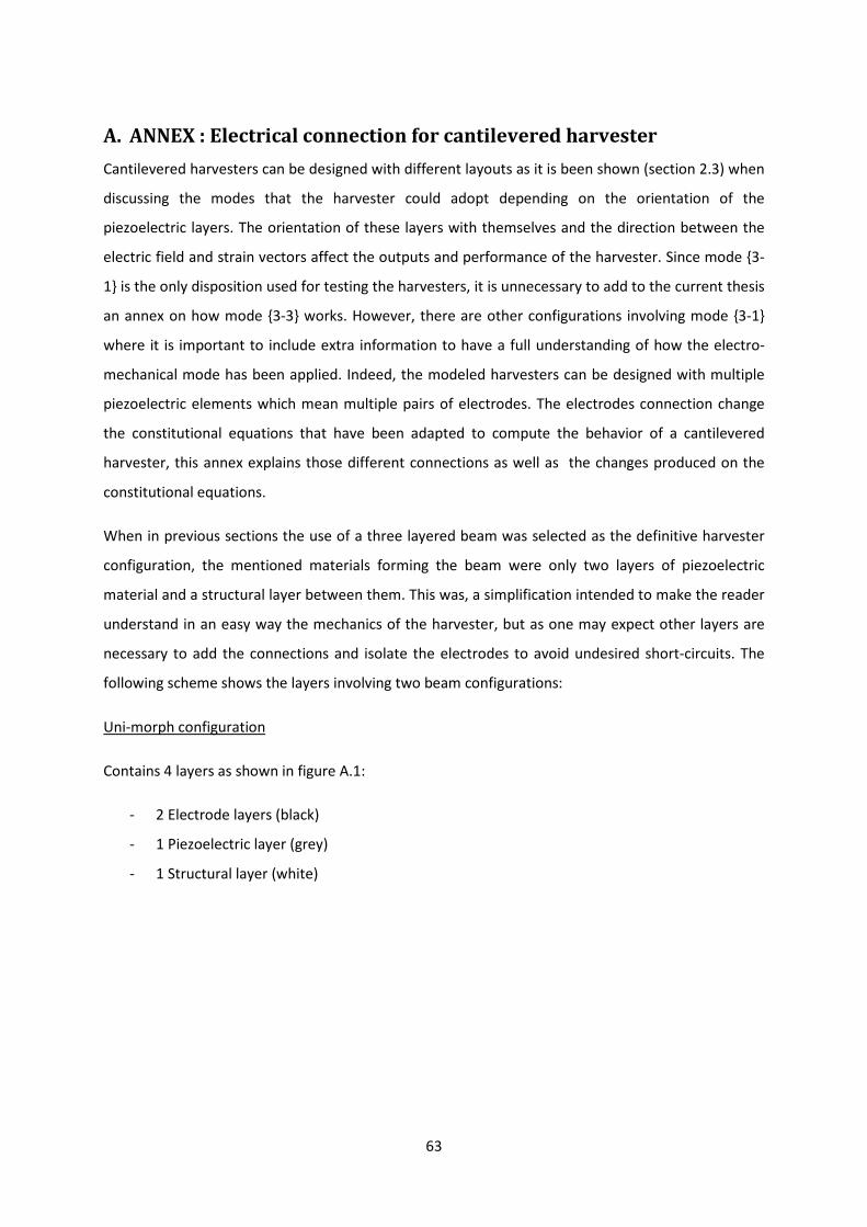
63
A. ANNEX : Electrical connection for cantilevered harvester
Cantilevered harvesters can be designed with different layouts as it is been shown (section 2.3) when
discussing the modes that the harvester could adopt depending on the orientation of the
piezoelectric layers. The orientation of these layers with themselves and the direction between the
electric field and strain vectors affect the outputs and performance of the harvester. Since mode 3-
1 is the only disposition used for testing the harvesters, it is unnecessary to add to the current thesis
an annex on how mode 3-3 works. However, there are other configurations involving mode 3-1
where it is important to include extra information to have a full understanding of how the electro-
mechanical mode has been applied. Indeed, the modeled harvesters can be designed with multiple
piezoelectric elements which mean multiple pairs of electrodes. The electrodes connection change
the constitutional equations that have been adapted to compute the behavior of a cantilevered
harvester, this annex explains those different connections as well as the changes produced on the
constitutional equations.
When in previous sections the use of a three layered beam was selected as the definitive harvester
configuration, the mentioned materials forming the beam were only two layers of piezoelectric
material and a structural layer between them. This was, a simplification intended to make the reader
understand in an easy way the mechanics of the harvester, but as one may expect other layers are
necessary to add the connections and isolate the electrodes to avoid undesired short-circuits. The
following scheme shows the layers involving two beam configurations:
Uni-morph configuration
Contains 4 layers as shown in figure A.1:
- 2 Electrode layers (black)
- 1 Piezoelectric layer (grey)
- 1 Structural layer (white)
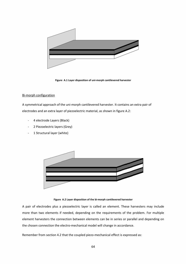
64
Figure A.1 Layer disposition of uni-morph cantilevered harvester
Bi-morph configuration
A symmetrical approach of the uni-morph cantilevered harvester. It contains an extra pair of
electrodes and an extra layer of piezoelectric material, as shown in figure A.2:
- 4 electrode Layers (Black)
- 2 Piezoelectric layers (Grey)
- 1 Structural layer (white)
Figure A.2 Layer disposition of the bi-morph cantilevered harvester
A pair of electrodes plus a piezoelectric layer is called an element. These harvesters may include
more than two elements if needed, depending on the requirements of the problem. For multiple
element harvesters the connection between elements can be in series or parallel and depending on
the chosen connection the electro-mechanical model will change in accordance.
Remember from section 4.2 that the coupled piezo-mechanical effect is expressed as:
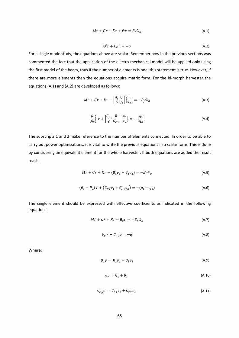
65
%)½ + )¬ + ) + Θ< = E½ (A.1)
Θ) + < = −( (A.2)
For a single mode study, the equations above are scalar. Remember how in the previous sections was
commented the fact that the application of the electro-mechanical model will be applied only using
the first model of the beam, thus if the number of elements is one, this statement is true. However, if
there are more elements then the equations acquire matrix form. For the bi-morph harvester the
equations (A.1) and (A.2) are developed as follows:
%)½ + )¬ + ) − ©Vo0 0Vpª <o<p = −E½ (A.3)
§VoVp¨ ) + ©ao0 0pª <o<p = − (o(p (A.4)
The subscripts 1 and 2 make reference to the number of elements connected. In order to be able to
carry out power optimizations, it is vital to write the previous equations in a scalar form. This is done
by considering an equivalent element for the whole harvester. If both equations are added the result
reads:
%)½ + )¬ + ) − θo<o + Vp<p = −E½ (A.5)
Vo + Vp) + ´o<o + p<pµ = −(o + (p (A.6)
The single element should be expressed with effective coefficients as indicated in the following
equations
%)½ + )¬ + ) − θ< = −E½ (A.7)
V ) + < = −( (A.8)
Where:
V< = θo<o + Vp<p (A.9)
V = θo + Vp (A.10)
a< = o<o + p<p (A.11)

66
Notice that for a single element harvester the equivalent scalar equation is reduced to the original
equations. Nevertheless, the charge (can be expressed in terms of the voltage using the relations
with intensity for single or multiple element harvesters:
= (8 ; = < (A.12)
V )¬ + <¬ + 1 < = 0 (A.13)
The next subsections will show how the equivalent terms are found assuming a symmetrical bi-
morph configuration14
A.1. Series connection
For the series connection, the two elements are poled in opposite directions, such as the strains
produced above and below the neutral axis generate electric fields that are in the same direction.
Figure A.3 shows the connection of the device (right) and the corresponding scheme on the left.
Figure A.3 Series connection for a bi-morph harvester
There are two observations two be noticed:
<o + <p = < (A.14)
(o = (p = ( (A.15)
Now substituting on the governing equations shown at the beginning of the section (expressions
(A.5) and (A.6)) leads to:
%)½ + )¬ + ) − 2θo<o = −E½ (A.16)
2Vo)¬ + 2o<o = −2(o (A.17)
14
Since Bi-morph configuration contains two elements is enough to show the dynamics of connecting various elements. For
more than two elements, the process would be analogous.
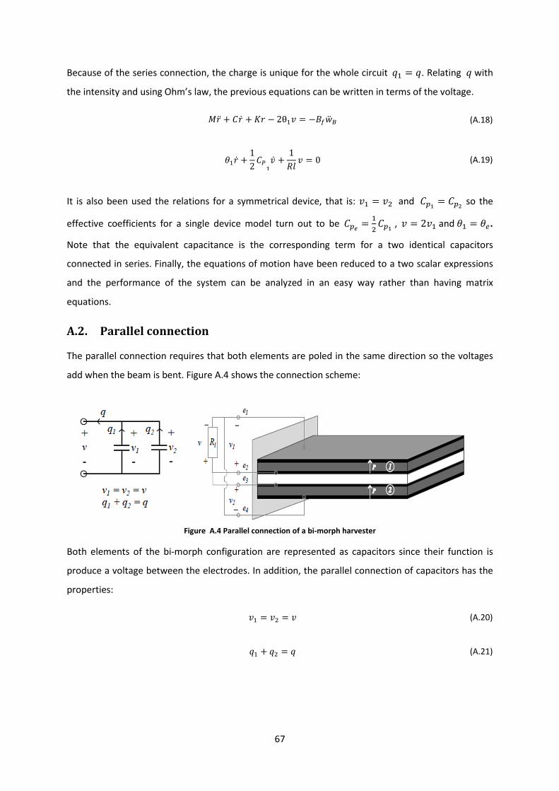
67
Because of the series connection, the charge is unique for the whole circuit(o = (. Relating (with
the intensity and using Ohm’s law, the previous equations can be written in terms of the voltage.
%)½ + )¬ + ) − 2θo< = −E½ (A.18)
Vo)¬ + 12
o
<¬ 1
< 0 (A.19)
It is also been used the relations for a symmetrical device, that is: <o <p and aw aÔ so the
effective coefficients for a single device model turn out to beaÞ o
paw , < 2<oandVo V.
Note that the equivalent capacitance is the corresponding term for a two identical capacitors
connected in series. Finally, the equations of motion have been reduced to a two scalar expressions
and the performance of the system can be analyzed in an easy way rather than having matrix
equations.
A.2. Parallel connection
The parallel connection requires that both elements are poled in the same direction so the voltages
add when the beam is bent. Figure A.4 shows the connection scheme:
Figure A.4 Parallel connection of a bi-morph harvester
Both elements of the bi-morph configuration are represented as capacitors since their function is
produce a voltage between the electrodes. In addition, the parallel connection of capacitors has the
properties:
<o <p < (A.20)
(o (p ( (A.21)

68
Introducing these two definitions in equations (A.5) and (A.6) both expressions are written in terms
of the voltage and charge. But then again, remembering the relations = 1³10 and < = the new
equations become a function of the voltage as happened with equations (A.7) and (A.13):
%)½ + )¬ + ) − θo + Vp< = −E½ (A.22)
Vo + Vp)¬ + ´o + pµ<¬ + 1 < = 0 (A.23)
For convenience, the effective coefficients are implemented in the single electrode system model,
being: V = Vo + Vp andaÞ = aw + aÔ.
Note that the results look intuitive since the effective capacitance for two capacitors in parallel
simply the sum of individual capacitances. If the bi-morph beam were symmetric (Vo = Vpandaw =aÔ) then the equivalent coefficient are rewrote as follows:
V = 2Vo = o (A.24)
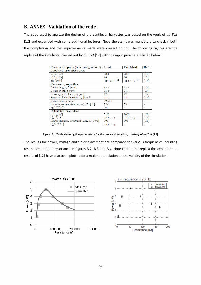
69
B. ANNEX : Validation of the code
The code used to analyze the design of the cantilever harvester was based on the work of du Toit
[12] and expanded with some additional features. Nevertheless, it was mandatory to check if both
the completion and the improvements made were correct or not. The following figures are the
replica of the simulation carried out by du Toit [12] with the input parameters listed below:
Figure B.1 Table showing the parameters for the device simulation, courtesy of du Toit [12].
The results for power, voltage and tip displacement are compared for various frequencies including
resonance and anti-resonance in figures B.2, B.3 and B.4. Note that in the replica the experimental
results of [12] have also been plotted for a major appreciation on the validity of the simulation.
0
1
2
3
4
5
6
0 100000 200000 300000
Po
we
r (µ
W)
Resistance (Ω)
Power f=70Hz
Mesured
Simulated

70
0
5
10
15
20
25
30
35
40
45
0 50000 100000 150000 200000 250000
Po
we
r (µ
W)
Resistance (Ω)
Power f=95Hz
Mesured
Simulated
0
100
200
300
400
500
600
700
0 100000 200000 300000
Po
we
r (µ
W)
Resistance (Ω)
Power f=107Hz (Resonance)
Mesured
Simulated
0
100
200
300
400
500
600
0 100000 200000 300000
Po
we
r (µ
W)
Resistance (Ω)
Power f=113Hz (Anti-resonance)
Mesured
Simulated

71
Figure B.2 Comparison of the Power output vs. resistive load for different frequencies. Thesis results on the left and
original simulation on the right
0
5
10
15
20
25
30
35
40
45
0 100000 200000 300000
Po
we
r (µ
W)
Resistance (Ω)
Power f=125Hz
Mesured
Simulated
0
1
2
3
4
5
6
7
0 100000 200000 300000
Po
we
r (µ
W)
Resistance (Ω)
Power f=150Hz
Mesured
Simulated
0
0,1
0,2
0,3
0,4
0,5
0,6
0,7
0 100000 200000 300000
Vo
lta
ge
(µ
V)
Resistance (Ω)
Voltage F=70 Hz

72
0
0,2
0,4
0,6
0,8
1
1,2
1,4
1,6
0 100000 200000 300000
Vo
lta
ge
(µ
V)
Resistance (Ω)
Voltage F=95Hz
0
0,5
1
1,5
2
2,5
3
3,5
4
0 100000 200000 300000
Vo
lta
ge
(µ
V)
Resistance (Ω)
Voltage F=107 Hz (Resonance)
Mesured
Simulated
0
1
2
3
4
5
6
7
8
9
10
0 100000 200000 300000
Vo
lta
ge
(µ
V)
Resistance (Ω)
Voltage F=113 Hz (Anti-resonance)
Mesured
Simulated
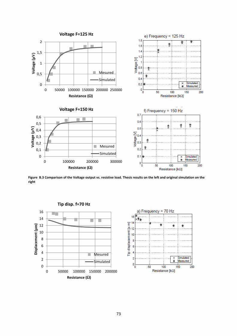
73
Figure B.3 Comparison of the Voltage output vs. resistive load. Thesis results on the left and original simulation on the
right
0
0,5
1
1,5
2
0 50000 100000 150000 200000 250000
Vo
lta
ge
(µ
V)
Resistance (Ω)
Voltage F=125 Hz
Mesured
Simulated
0
0,1
0,2
0,3
0,4
0,5
0,6
0 100000 200000 300000
Vo
lta
ge
(µ
V)
Resistance (Ω)
Voltage F=150 Hz
Mesured
Simulated
0
2
4
6
8
10
12
14
16
0 50000 100000 150000 200000
Dis
pla
cem
en
t (µ
m)
Resistance (Ω)
Tip disp. f=70 Hz
Mesured
Simulated
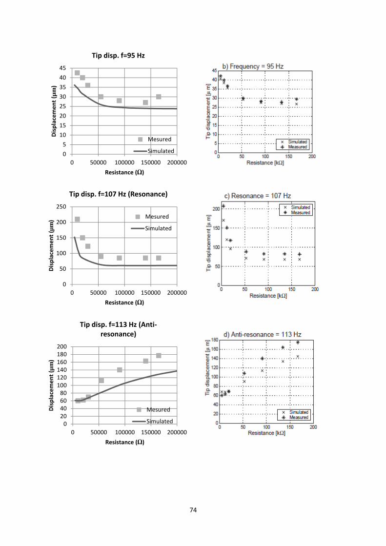
74
0
5
10
15
20
25
30
35
40
45
0 50000 100000 150000 200000
Dis
pla
cem
en
t (µ
m)
Resistance (Ω)
Tip disp. f=95 Hz
Mesured
Simulated
0
50
100
150
200
250
0 50000 100000 150000 200000
Dis
pla
cem
en
t (µ
m)
Resistance (Ω)
Tip disp. f=107 Hz (Resonance)
Mesured
Simulated
0
20
40
60
80
100
120
140
160
180
200
0 50000 100000 150000 200000
Dis
pla
cem
en
t (µ
m)
Resistance (Ω)
Tip disp. f=113 Hz (Anti-
resonance)
Mesured
Simulated
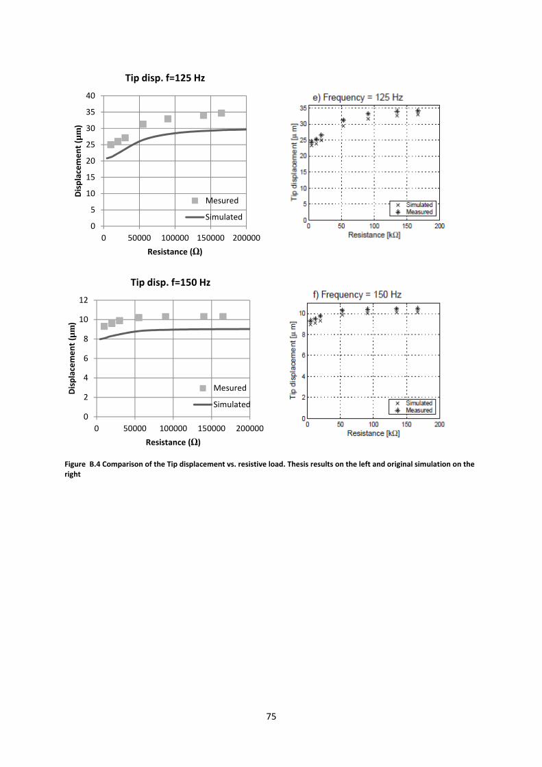
75
Figure B.4 Comparison of the Tip displacement vs. resistive load. Thesis results on the left and original simulation on the
right
0
5
10
15
20
25
30
35
40
0 50000 100000 150000 200000
Dis
pla
cem
en
t (µ
m)
Resistance (Ω)
Tip disp. f=125 Hz
Mesured
Simulated
0
2
4
6
8
10
12
0 50000 100000 150000 200000
Dis
pla
cem
en
t (µ
m)
Resistance (Ω)
Tip disp. f=150 Hz
Mesured
Simulated
Top Related