


Languages
Pages
Legal


Artificial Intelligence Planning
Graphplan
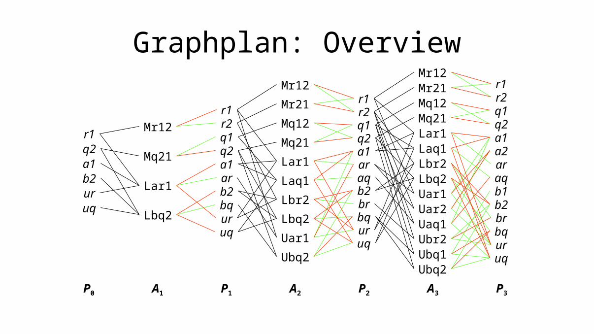
Graphplan: Overview
r1q2a1b2uruq
r1r2q1q2a1arb2bquruq
r1r2q1q2a1ar
b2
bquruq
aq
br
r1r2q1q2a1
ar
b2
bquruq
aq
br
a2
b1
Mr12
Mq21
Lbq2
Lar1
Mr12
Mq21
Lbr2
Lar1
Mr21
Mq12
Lbq2
Laq1
Uar1
Ubq2
Mr12
Mq21
Lbr2
Lar1
Mr21Mq12
Lbq2
Laq1
Uar1
Ubq2
Uar2
Ubq1
Uaq1Ubr2
P0 A1 P3P2P1 A3A2

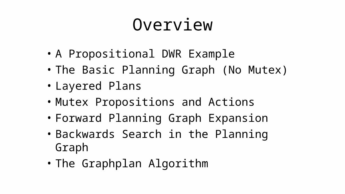
Overview
• A Propositional DWR Example
• The Basic Planning Graph (No Mutex)
• Layered Plans
• Mutex Propositions and Actions
• Forward Planning Graph Expansion
• Backwards Search in the Planning Graph
• The Graphplan Algorithm
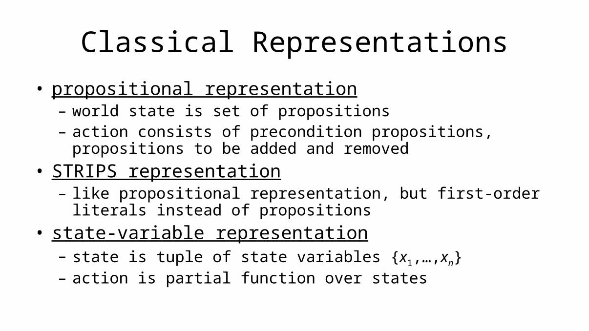
Classical Representations
• propositional representation– world state is set of propositions– action consists of precondition propositions, propositions to be added
and removed
• STRIPS representation– like propositional representation, but first-order literals instead of
propositions
• state-variable representation– state is tuple of state variables {x1,…,xn}– action is partial function over states
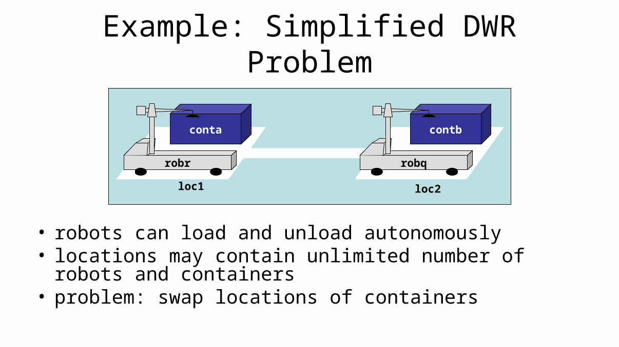
Example: Simplified DWR Problem
• robots can load and unload autonomously• locations may contain unlimited number of robots and
containers• problem: swap locations of containers
loc1 loc2
conta
robr
contb
robq

Simplified DWR Problem: STRIPS Operators
• move(r,l,l’)– precond: at(r,l), adjacent(l,l’)– effects: at(r,l’), ¬at(r,l)
• load(c,r,l)– precond: at(r,l), in(c,l), unloaded(r)– effects: loaded(r,c), ¬in(c,l), ¬unloaded(r)
• unload(c,r,l)– precond: at(r,l), loaded(r,c)– effects: unloaded(r), in(c,l), ¬loaded(r,c)

Simplified DWR Problem: State Proposition Symbols
• robots:– r1 and r2: at(robr,loc1) and at(robr,loc2)– q1 and q2: at(robq,loc1) and at(robq,loc2)– ur and uq: unloaded(robr) and unloaded(robq)
• containers:– a1, a2, ar, and aq: in(conta,loc1), in(conta,loc2), loaded(conta,robr),
and loaded(conta,robq)– b1, b2, br, and bq: in(contb,loc1), in(contb,loc2), loaded(contb,robr),
and loaded(contb,robq)
• initial state: {r1, q2, a1, b2, ur, uq}

Simplified DWR Problem: Action Symbols
• move actions:– Mr12: move(robr,loc1,loc2), Mr21: move(robr,loc2,loc1), Mq12:
move(robq,loc1,loc2), Mq21: move(robq,loc2,loc1)
• load actions:– Lar1: load(conta,robr,loc1); Lar2, Laq1, Laq2, Lbr1, Lbr2, Lbq1, and
Lbq2 correspondingly
• unload actions:– Uar1: unload(conta,robr,loc1); Uar2, Uaq1, Uaq2, Ubr1, Ubr2, Ubq1,
and Ubq2 correspondingly

Overview
• A Propositional DWR Example
• The Basic Planning Graph (No Mutex)
• Layered Plans
• Mutex Propositions and Actions
• Forward Planning Graph Expansion
• Backwards Search in the Planning Graph
• The Graphplan Algorithm

Solution Existence
• Proposition: A propositional planning problem P=(Σ,si,g) has a solution iff
Sg ⋂ Γ>({si}) ≠ {}.
• Proposition: A propositional planning problem P=(Σ,si,g) has a solution iff
∃s∈Γ<({g}) : s⊆si.
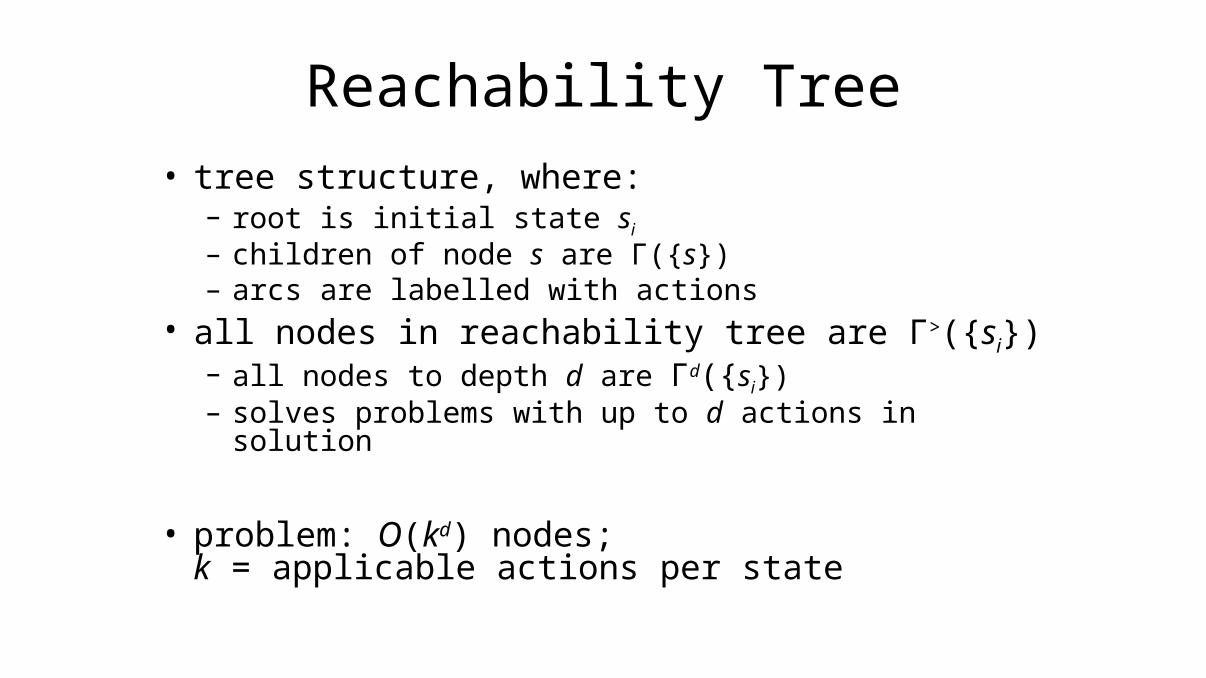
Reachability Tree
• tree structure, where:– root is initial state si
– children of node s are Γ({s})– arcs are labelled with actions
• all nodes in reachability tree are Γ>({si}) – all nodes to depth d are Γd({si}) – solves problems with up to d actions in solution
• problem: O(kd) nodes; k = applicable actions per state
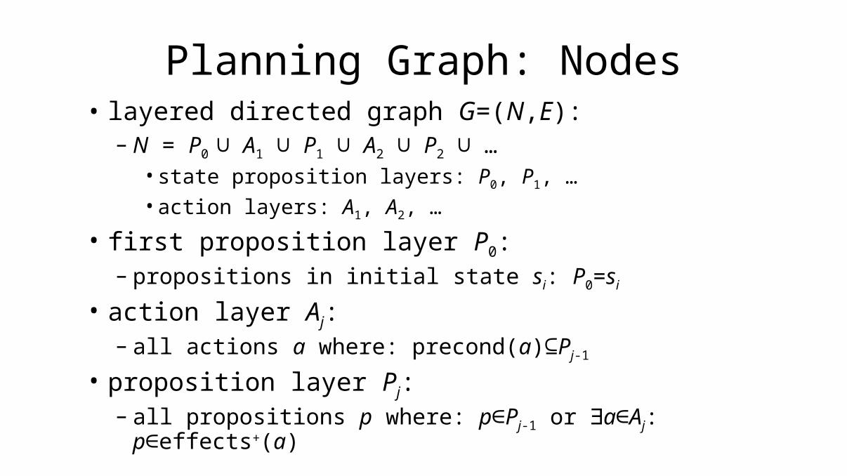
Planning Graph: Nodes• layered directed graph G=(N,E):
– N = P0 ∪ A1 ∪ P1 ∪ A2 ∪ P2 ∪ … • state proposition layers: P0, P1, …• action layers: A1, A2, …
• first proposition layer P0:– propositions in initial state si: P0=si
• action layer Aj:– all actions a where: precond(a)⊆Pj-1
• proposition layer Pj:– all propositions p where: p∈Pj-1 or ∃a∈Aj: p∈effects+(a)
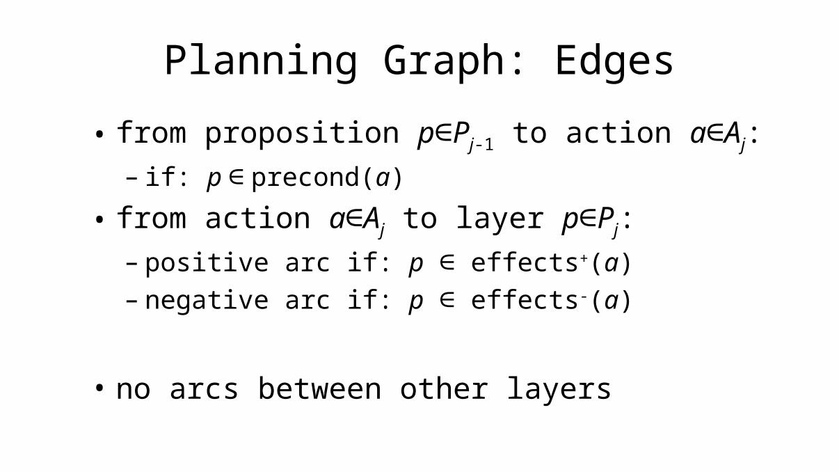
Planning Graph: Edges
• from proposition p∈Pj-1 to action a∈Aj:
– if: p ∈ precond(a)
• from action a∈Aj to layer p∈Pj:
– positive arc if: p ∈ effects+(a)– negative arc if: p ∈ effects-(a)
• no arcs between other layers

Planning Graph Example
r1q2a1b2uruq
r1r2q1q2a1arb2bquruq
r1r2q1q2a1ar
b2
bquruq
aq
br
r1r2q1q2a1
ar
b2
bquruq
aq
br
a2
b1
Mr12
Mq21
Lbq2
Lar1
Mr12
Mq21
Lbr2
Lar1
Mr21
Mq12
Lbq2
Laq1
Uar1
Ubq2
Mr12
Mq21
Lbr2
Lar1
Mr21Mq12
Lbq2
Laq1
Uar1
Ubq2
Uar2
Ubq1
Uaq1Ubr2
P0 A1 P3P2P1 A3A2

Reachability in the Planning Graph
• reachability analysis:– if a goal g is reachable from initial state si
– then there will be a proposition layer Pg in the planning graph such that g⊆Pg
• necessary condition, but not sufficient• low complexity:
– planning graph is of polynomial size and – can be computed in polynomial time

Overview
• A Propositional DWR Example
• The Basic Planning Graph (No Mutex)
• Layered Plans
• Mutex Propositions and Actions
• Forward Planning Graph Expansion
• Backwards Search in the Planning Graph
• The Graphplan Algorithm

Independent Actions: Examples• Mr12 and Lar1:
– cannot occur together– Mr12 deletes precondition r1 of Lar1
• Mr12 and Mr21:– cannot occur together– Mr12 deletes positive effect r1 of
Mr21• Mr12 and Mq21:
– may occur in same action layer
r1r2q1q2a1arb2bquruq
r1r2q1q2a1ar
b2
bquruq
aq
br
Mr12
Mq21
Lbr2
Lar1
Mr21
Mq12
Lbq2
Laq1
Uar1
Ubq2
P2P1 A2
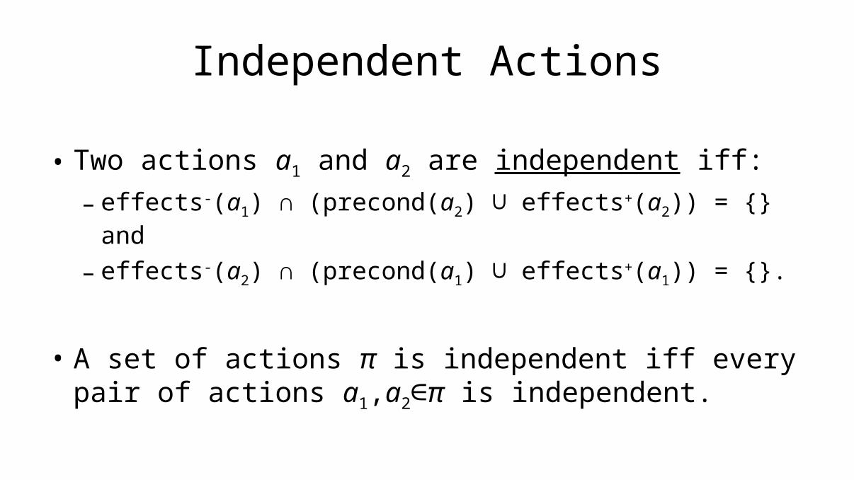
Independent Actions
• Two actions a1 and a2 are independent iff:
– effects-(a1) ∩ (precond(a2) ∪ effects+(a2)) = {} and
– effects-(a2) ∩ (precond(a1) ∪ effects+(a1)) = {}.
• A set of actions π is independent iff every pair of actions a1,a2∈π is independent.

Pseudo Code: independent
function independent(a1,a2)
for all p∈effects-(a1)
if p∈precond(a2) or p∈effects+(a2) then
return false
for all p∈effects-(a2)
if p∈precond(a1) or p∈effects+(a1) then
return false
return true
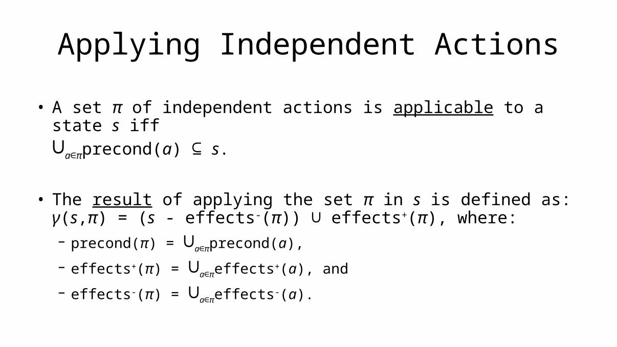
Applying Independent Actions
• A set π of independent actions is applicable to a state s iff
∪a∈πprecond(a) ⊆ s.
• The result of applying the set π in s is defined as:γ(s,π) = (s - effects-(π)) ∪ effects+(π), where:– precond(π) = ∪a∈πprecond(a),
– effects+(π) = ∪a∈πeffects+(a), and
– effects-(π) = ∪a∈πeffects-(a).
Execution Order of Independent Actions
• Proposition: If a set π of independent actions is applicable in state s then, for any permutation ⟨a1,…,ak of the elements of ⟩ π: – the sequence ⟨a1,…,ak is applicable to ⟩ s, and– the state resulting from the application of π to s is the same
as from the application of ⟨a1,…,ak , i.e.:⟩γ(s,π) = γ(s,⟨a1,…,ak⟩).
Layered Plans
• Let P = (A,si,g) be a statement of a propositional planning problem and G = (N,E), N = P0 ∪ A1 ∪ P1 ∪ A2 ∪ P2 ∪ …, the corresponding planning graph.
• A layered plan over G is a sequence of sets of actions: ∏ = ⟨π1,…,πk where: ⟩– πi ⊆ Ai ⊆ A,
– πi is applicable in state Pi-1, and
– the actions in πi are independent.
Layered Solution Plan
• A layered plan ∏ = ⟨π1,…,πk⟩ is a solution to a to a planning problem P=(A,si,g) iff:
– π1 is applicable in si,
– for j∈{2…k}, πj is applicable in state γ(…γ(γ(si,π1), π2), … πj-1), and
– g ⊆ γ(…γ(γ(si,π1), π2), …, πk).

Overview
• A Propositional DWR Example
• The Basic Planning Graph (No Mutex)
• Layered Plans
• Mutex Propositions and Actions
• Forward Planning Graph Expansion
• Backwards Search in the Planning Graph
• The Graphplan Algorithm

Problem: Dependent Propositions: Example
• r2 and ar: – r2: positive effect of Mr12– ar: positive effect of Lar1– but: Mr12 and Lar1 not independent– hence: r2 and ar incompatible in P1
• r1 and r2:– positive and negative effects of same
action: Mr12– hence: r1 and r2 incompatible in P1
r1q2a1b2uruq
r1r2q1q2a1arb2bquruq
P0 A1 P1
Mr12
Mq21
Lbq2
Lar1

No-Operation Actions
• No-Op for proposition p:– name: Ap– precondition: p– effect: p
• r1 and r2:– r1: positive effect of Ar1– r2: positive effect of Mr12– but: Ar1 and Mr12 not independent– hence: r1 and r2 incompatible in P1
• only one incompatibility test
Mr12
Mq21
Lbq2
Lar1
r1r2q1q2a1arb2bquruq
r1q2a1b2uruq
P0 A1 P1
Ar1

Mutex Propositions
• Two propositions p and q in proposition layer Pj are mutex (mutually exclusive) if:– every action in the preceding action layer Aj that has p as a
positive effect (incl. no-op actions) is mutex with every action in Aj that has q as a positive effect, and
– there is no single action in Aj that has both, p and q, as positive effects.
• notation: μPj = { (p,q) | p,q∈Pj are mutex}
Pseudo Code: mutex for Propositions
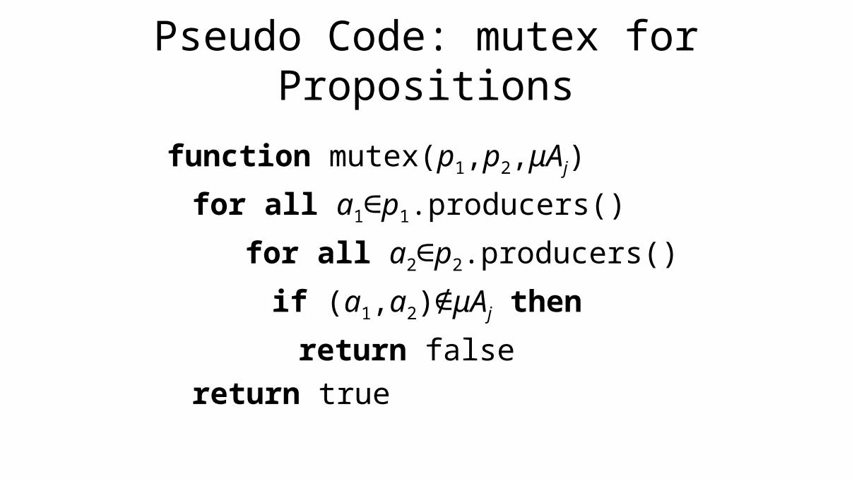
function mutex(p1,p2,μAj)
for all a1∈p1.producers()
for all a2∈p2.producers()
if (a1,a2)∉μAj then
return false
return true
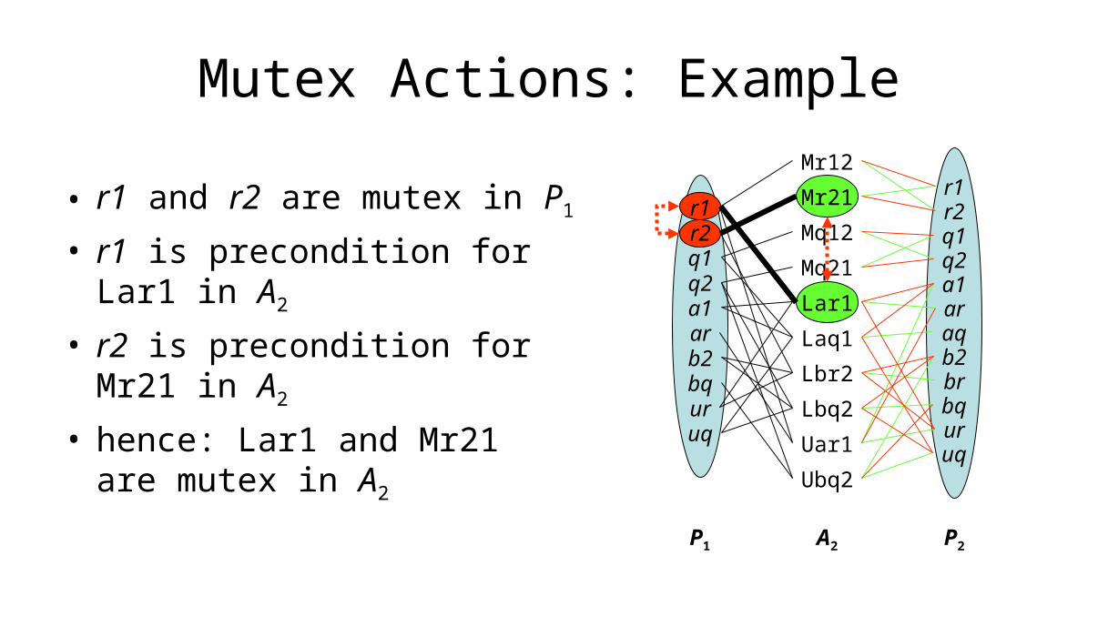
Mutex Actions: Example
• r1 and r2 are mutex in P1
• r1 is precondition for Lar1 in A2
• r2 is precondition for Mr21 in A2
• hence: Lar1 and Mr21 are mutex in A2
r1r2q1q2a1arb2bquruq
r1r2q1q2a1ar
b2
bquruq
aq
br
Mr12
Mq21
Lbr2
Lar1
Mr21
Mq12
Lbq2
Laq1
Uar1
Ubq2
P2P1 A2
Mutex Actions
• Two actions a1 and a2 in action layer Aj are mutex if:
– a1 and a2 are dependent, or
– a precondition of a1 is mutex with a precondition of a2.
• notation: μAj = { (a1,a2) | a1,a2 ∈Aj are mutex}

Pseudo Code: mutex for Actions
function mutex(a1,a2,μP)
if ¬independent(a1,a2) then
return true
for all p1∈precond(a1)
for all p2∈precond(a2)
if (p1,p2)∈μP then return true
return false

Decreasing Mutex Relations• Proposition: If p,q∈Pj-1 and (p,q)∉μPj-1 then (p,q)∉μPj.
– Proof: • if p,q∈Pj-1 then Ap,Aq∈Aj
• if (p,q)∉μPj-1 then (Ap,Aq)∉μAj
• since Ap,Aq∈Aj and (Ap,Aq)∉μAj, (p,q)∉μPj must hold
• Proposition: If a1,a2∈Aj-1 and (a1,a2)∉μAj-1 then (a1,a2)∉μAj.
– Proof:• if a1,a2∈Aj-1 and (a1,a2)∉μAj-1 then
– a1 and a2 are independent and
– their preconditions in Pj-1 are not mutex
• both properties remain true for Pj
• hence: a1,a2∈Aj and (a1,a2)∉μAj
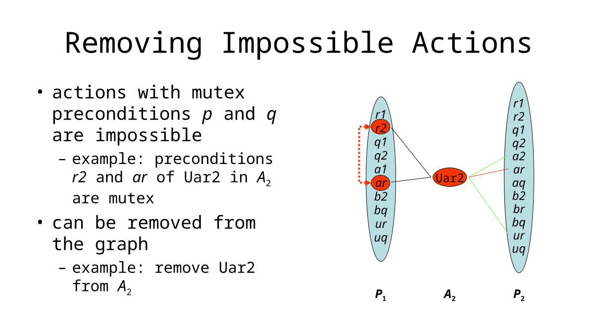
Removing Impossible Actions
• actions with mutex preconditions p and q are impossible– example: preconditions r2 and
ar of Uar2 in A2 are mutex
• can be removed from the graph– example: remove Uar2 from A2
r1r2q1q2a1arb2bquruq
r1r2q1q2a2ar
b2
bquruq
aq
br
Uar2
P2P1 A2
Overview
• A Propositional DWR Example
• The Basic Planning Graph (No Mutex)
• Layered Plans
• Mutex Propositions and Actions
• Forward Planning Graph Expansion
• Backwards Search in the Planning Graph
• The Graphplan Algorithm
Reachability in Planning Graphs
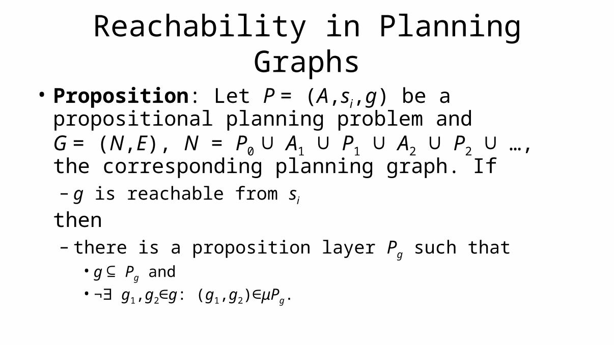
• Proposition: Let P = (A,si,g) be a propositional planning problem and G = (N,E), N = P0 ∪ A1 ∪ P1 ∪ A2 ∪ P2 ∪ …, the corresponding planning graph. If – g is reachable from si
then – there is a proposition layer Pg such that
• g ⊆ Pg and• ¬∃ g1,g2∈g: (g1,g2)∈μPg.

The Graphplan Algorithm: Basic Idea
• expand the planning graph, one action layer and one proposition layer at a time
• from the first graph for which Pg is the last proposition layer such that – g ⊆ Pg and– ¬∃ g1,g2∈g: (g1,g2)∈μPg
• search backwards from the last (proposition) layer for a solution
Planning Graph Data Structure
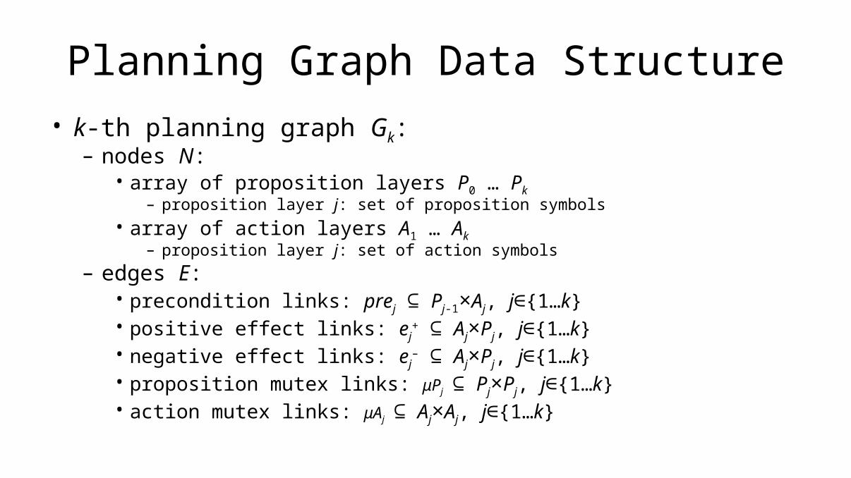
• k-th planning graph Gk:– nodes N:
• array of proposition layers P0 … Pk– proposition layer j: set of proposition symbols
• array of action layers A1 … Ak– proposition layer j: set of action symbols
– edges E:• precondition links: prej ⊆ Pj-1×Aj, j∈{1…k}• positive effect links: ej
+ ⊆ Aj×Pj, j∈{1…k}• negative effect links: ej
– ⊆ Aj×Pj, j∈{1…k}• proposition mutex links: μPj ⊆ Pj×Pj, j∈{1…k}• action mutex links: μAj ⊆ Aj×Aj, j∈{1…k}
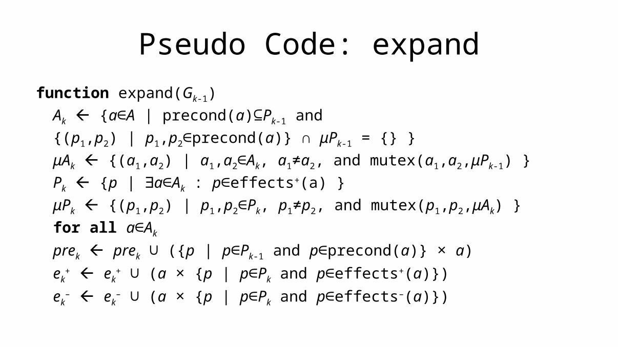
Pseudo Code: expand
function expand(Gk-1)
Ak {a∈A | precond(a)⊆Pk-1 and
{(p1,p2) | p1,p2∈precond(a)} ∩ μPk-1 = {} }
μAk {(a1,a2) | a1,a2∈Ak, a1≠a2, and mutex(a1,a2,μPk-1) }
Pk {p | ∃a∈Ak : p∈effects+(a) }
μPk {(p1,p2) | p1,p2∈Pk, p1≠p2, and mutex(p1,p2,μAk) }
for all a∈Ak
prek prek ∪ ({p | p∈Pk-1 and p∈precond(a)} × a)
ek+ ek
+ ∪ (a × {p | p∈Pk and p∈effects+(a)})
ek– ek
– ∪ (a × {p | p∈Pk and p∈effects–(a)})
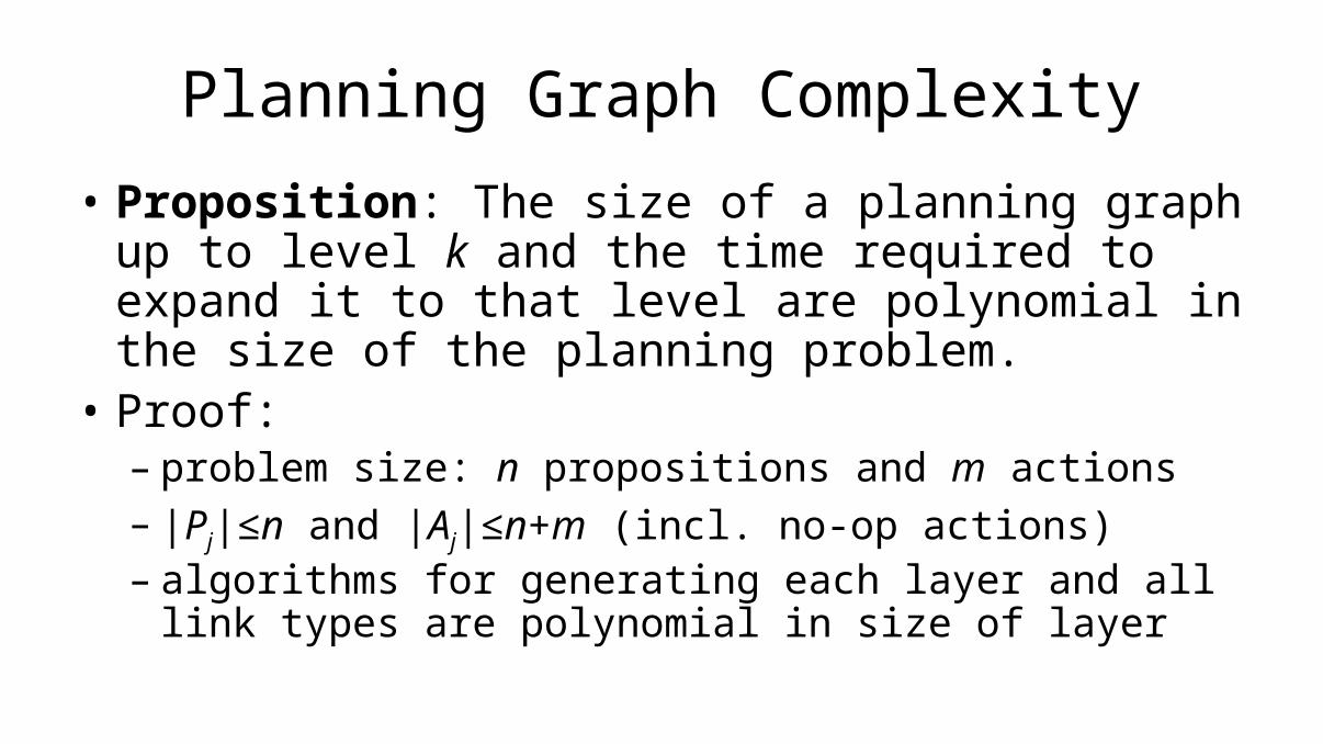
Planning Graph Complexity
• Proposition: The size of a planning graph up to level k and the time required to expand it to that level are polynomial in the size of the planning problem.
• Proof: – problem size: n propositions and m actions– |Pj|≤n and |Aj|≤n+m (incl. no-op actions) – algorithms for generating each layer and all link types are
polynomial in size of layer
Fixed-Point Levels
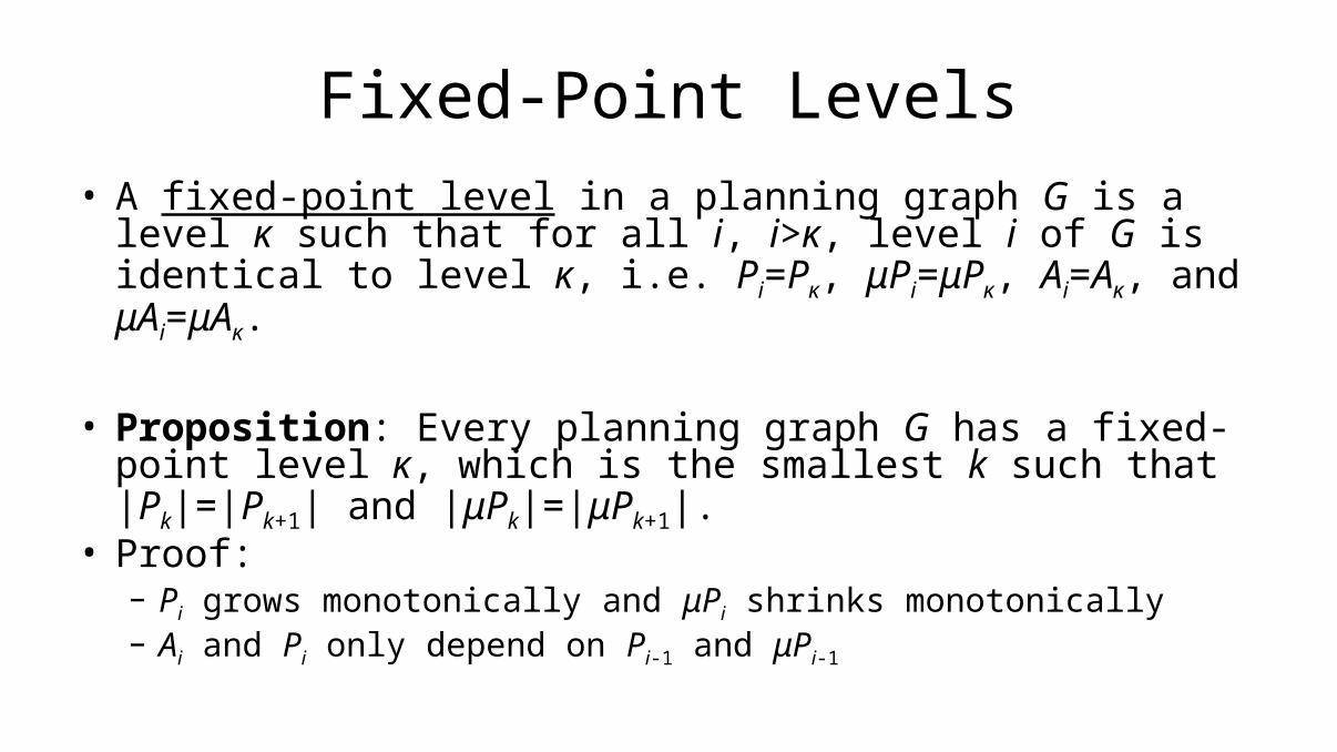
• A fixed-point level in a planning graph G is a level κ such that for all i, i>κ, level i of G is identical to level κ, i.e. Pi=Pκ, μPi=μPκ, Ai=Aκ, and μAi=μAκ.
• Proposition: Every planning graph G has a fixed-point level κ, which is the smallest k such that |Pk|=|Pk+1| and |μPk|=|μPk+1|.
• Proof:– Pi grows monotonically and μPi shrinks monotonically– Ai and Pi only depend on Pi-1 and μPi-1

Overview
• A Propositional DWR Example
• The Basic Planning Graph (No Mutex)
• Layered Plans
• Mutex Propositions and Actions
• Forward Planning Graph Expansion
• Backwards Search in the Planning Graph
• The Graphplan Algorithm
Searching the Planning Graph
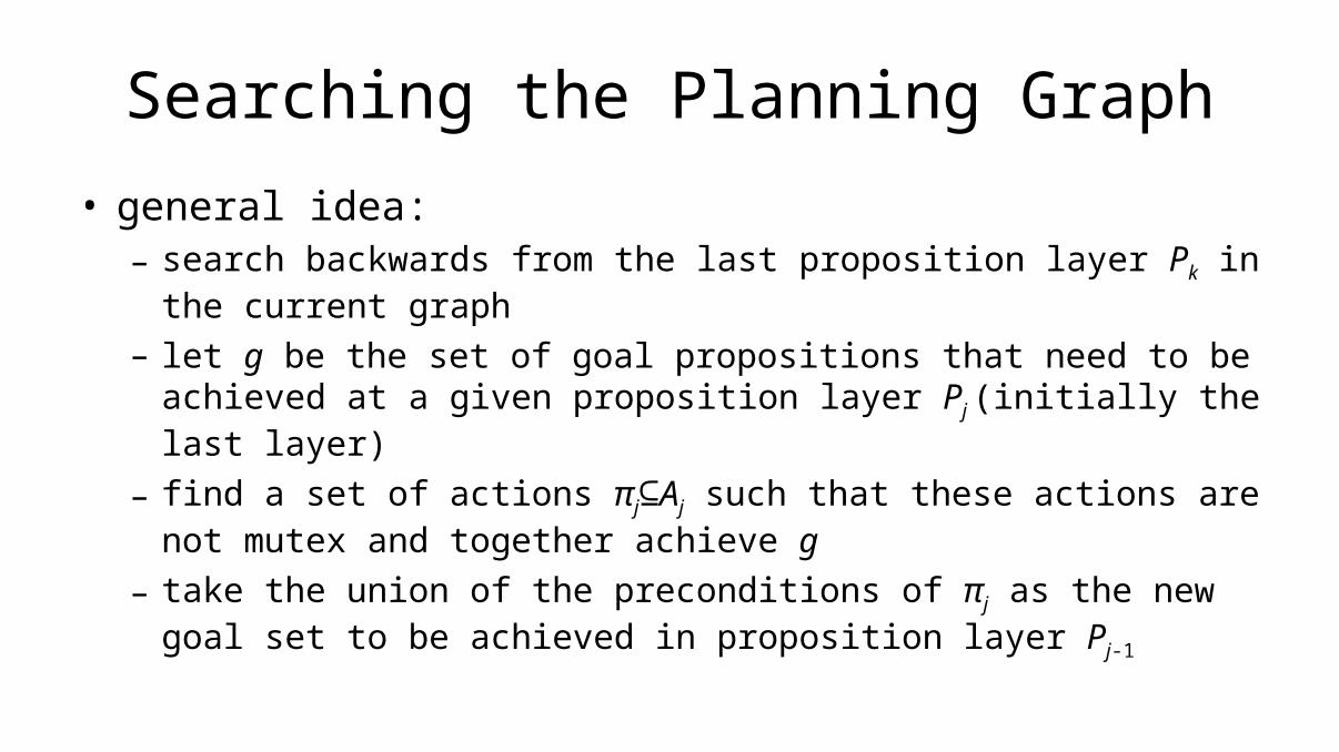
• general idea:– search backwards from the last proposition layer Pk in the current
graph– let g be the set of goal propositions that need to be achieved at a
given proposition layer Pj (initially the last layer)
– find a set of actions πj⊆Aj such that these actions are not mutex and together achieve g
– take the union of the preconditions of πj as the new goal set to be achieved in proposition layer Pj-1
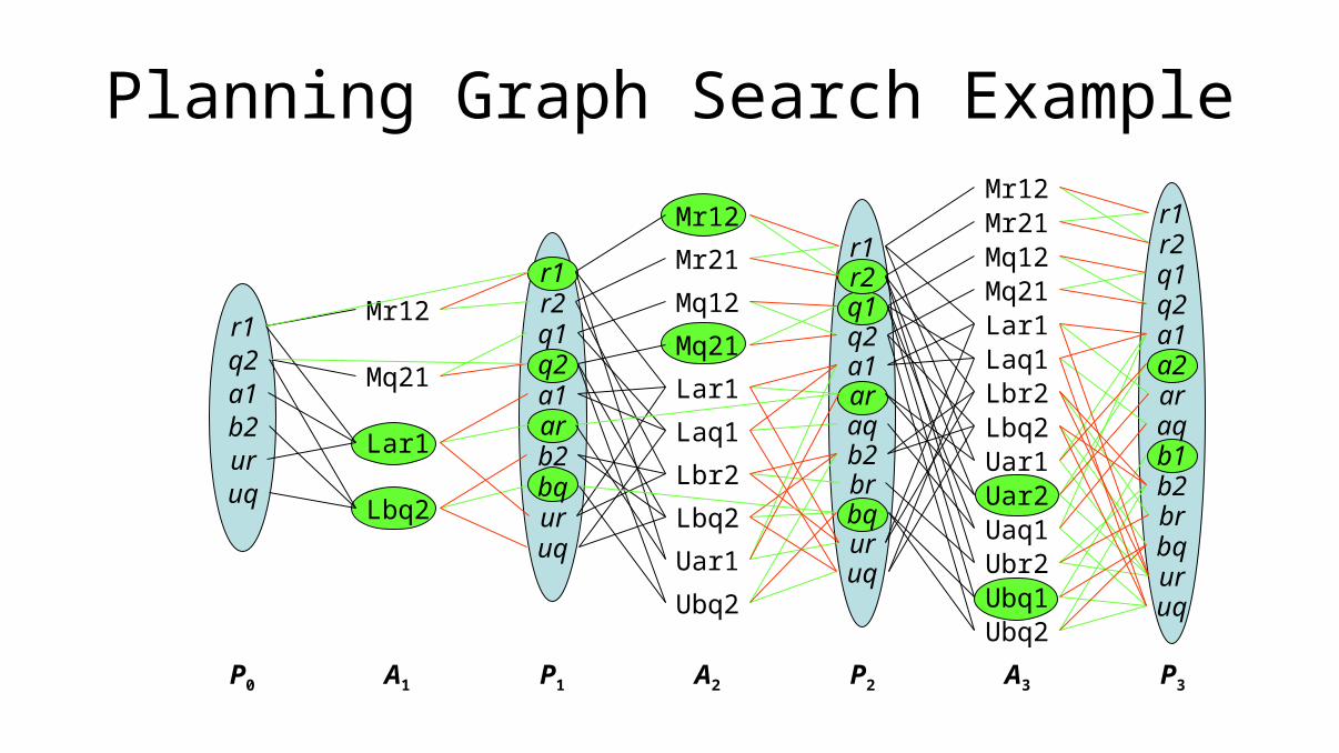
Planning Graph Search Example
a2
b1Uar1
r1q2a1b2uruq
r1r2q1q2a1arb2bquruq
r1r2q1q2a1ar
b2
bquruq
aq
br
r1r2q1q2a1
ar
b2
bquruq
aq
br
Mr12
Mq21
Lbq2
Lar1
Mr12
Mq21
Lbr2
Lar1
Mr21
Mq12
Lbq2
Laq1
Uar1
Ubq2
Mr12
Mq21
Lbr2
Lar1
Mr21Mq12
Lbq2
Laq1
Ubq2
Uar2
Ubq1
Uaq1Ubr2
P0 A1 P3P2P1 A3A2
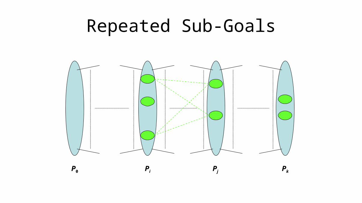
Repeated Sub-Goals
P0 Pi Pj
Pk

The nogood Table
• nogood table (denoted ∇) for planning graph up to layer k:– array of k sets of sets of goal propositions
• inner set: one combination of propositions that cannot be achieved• outer set: all combinations that cannot be achieved (at that layer)
• before searching for set g in Pj:– check whether g∈∇(j)
• when search for set g in Pj has failed:– add g to ∇(j)

Pseudo Code: extract
function extract(G,g,i)
if i=0 then return ⟨⟩
if g∈∇(i) then return failure
∏ gpSearch(G,g,{},i)
if ∏≠failure then return ∏
∇(i) ∇(i) + g
return failure

Pseudo Code: gpSearch
function gpSearch(G,g,π,i)if g={} then
∏ extract(G,∪a∈πprecond(a),i-1)if ∏ =failure then return failurereturn ∏ ∙⟨π⟩
p g.selectOne()providers {a∈Ai | p∈effects+(a) and ¬∃a’∈π: (a,a’)∈μAi}if providers={} then return failurea providers.chooseOne()return gpSearch(G,g-effects+(a),π+a,i)

Overview
• A Propositional DWR Example
• The Basic Planning Graph (No Mutex)
• Layered Plans
• Mutex Propositions and Actions
• Forward Planning Graph Expansion
• Backwards Search in the Planning Graph
• The Graphplan Algorithm

Pseudo Code: Graphplanfunction graphplan(A,si,g)
i 0; ∇ []; P0 si; G (P0,{})while (g⊈Pi or g2∩μPi≠{}) and ¬fixedPoint(G) do
i i+1; expand(G)if g⊈Pi or g2∩μPi≠{} then return failureη fixedPoint(G) ? |∇(κ)| : 0∏ extract(G,g,i)while ∏=failure do
i i+1; expand(G)∏ extract(G,g,i)if ∏=failure and fixedPoint(G) then
if η=|∇(κ)| then return failureη |∇(κ)|
return ∏

Graphplan Properties
• Proposition: The Graphplan algorithm is sound, complete, and always terminates. – It returns failure iff the given planning problem has no
solution; – otherwise, it returns a layered plan ∏ that is a solution to
the given planning problem.
• Graphplan is orders of magnitude faster than previous techniques!

Overview
• A Propositional DWR Example
• The Basic Planning Graph (No Mutex)
• Layered Plans
• Mutex Propositions and Actions
• Forward Planning Graph Expansion
• Backwards Search in the Planning Graph
• The Graphplan Algorithm
Top Related