


Languages
Pages
Legal

April 2005
ARCH Models for Multi-period Forecast Uncertainty
-A Reality Check Using a Panel of Density Forecasts
by
Kajal Lahiri and Fushang Liu Department of Economics
University at Albany – SUNY Albany, NY 12222. USA
Email: [email protected]
1
ARCH Models for Multi-period Forecast Uncertainty
-A Reality Check Using a Panel of Density Forecasts
Kajal Lahiri and Fushang Liu
Abstract
We develop a theoretical framework to compare forecast uncertainty estimated from time
series models to those available from survey density forecasts. The sum of the average
variance of individual densities and the disagreement, which is the same as the variance
of the aggregate density, is shown to approximate the predictive uncertainty from well
specified time series models when the variance of the aggregate shocks is relatively small
compared to that of the idiosyncratic shocks. We argue that due to grouping error
problems, compositional effects of the panel, and other complications, the uncertainty
measure has to be estimated from individual densities. Despite numerous reservations on
the credibility of time series based measures of forecast uncertainty, we found that during
normal times the uncertainty estimates based on ARCH models simulate the subjective
survey measure remarkably well. However, during times of regime change and structural
break, the two estimates do not overlap. We suggest ways to improve the time series
measures during periods when forecast errors are apt to be large. The disagreement series
is a good indicator of such periods.
Keywords: Inflation, Survey of Professional Forecasters, GARCH, Real time data.
JEL:E31; E37; C23; C53
2

1. Introduction
Macroeconomic uncertainty as characterized by aggregate forecast density or intervals
has long been recognized as an important factor in determining economic outcomes.1
Milton Friedman, in his Nobel lecture (1977), conjectured that high inflation causes high
inflation uncertainty, and that high uncertainty in turn causes inefficiencies in the
economy. The latest Nobel laureate Robert Engle (1983) wrote while introducing his
celebrated ARCH model,
“When inflation is unpredictable, risk averse economic agents will incur loss,
even if prices and quantities are perfectly flexible in all markets. Inflation
is a measure of the relative price of goods today and goods tomorrow;
thus, uncertainty in tomorrow’s price impairs the efficiency of today’s
allocation decisions.”
Not surprisingly, these developments have triggered much research studying the effects
of inflation uncertainty on savings, interest rates, investment, and other variables. More
recently, the introduction of inflation targeting regimes in U.K., Canada, Sweden, and
many other countries during the 1990s has rekindled an enormous interest in generating
credible inflation forecasts and the uncertainty associated with the forecasts.2
In order to deal with the causes and consequences of forecast uncertainty in a convincing
way, it has to be measured correctly. This is particularly important for predictive
uncertainty because, unlike forecasts, variance of predictive errors generated by macro
time series models is always unobserved, and hence, can never be evaluated against
subsequently observed realizations. During last twenty years, the most popular approach
to estimate forecast uncertainty has been the univariate or multivariate ARCH models
initiated by Engle (1982, 1983), who modeled the conditional variance of inflation
forecast error as an autoregressive conditional heteroskedastic (ARCH) process.
Bollerslev (1986), Nelson (1991), Glosten et al. (1993) and others have generalized the
1 Interval and probability forecasts have a longer track record in weather forecasts and sports picks. 2 See, for, instance, Sims (2002), Šmidková (2003), Cogley et al. (2003), and Garratt et al. (2003).
3

basic ARCH model in various directions, and have found many applications in finance
and economics.
There are, however, several possible reasons why ARCH-type models may not produce a
reliable proxy for inflation uncertainty. First, the reliability of this measure depends on
the reliability of the conditional mean and variance functions. This is why Engle (1982,
1983) had emphasized the need for various specification tests in these models. More
generally, Rich and Tracy (2003) have questioned the use of conditional variance of a
series which is essentially related to its ex post predictability as a measure of forecast
uncertainty which is related to ex ante confidence of a prediction. Second, most ARCH-
type models assume that the regime characterizing inflation and inflation uncertainty is
invariant over time. This assumption may not be true due to structural breaks. Although
some researchers have tried to rectify this deficiency (see, for example, Evans (1991),
Evans and Wachtel (1993)), the success of these efforts relies on correctly specifying the
structural break itself. Third, as noted by Bomberger (1996) and McNees (1989),
forecasters use different models. Thus, uncertainty regarding the model that generates
inflation may be a large part of inflation forecast uncertainty. Conditional variance
generated by a single model cannot capture this important feature. Finally, Zarnowitz and
Lambros (1987) observed that forecast uncertainty depends not only on past forecast
errors but also on many future-oriented factors such as policy changes, macro shocks,
data revisions and many others including purely subjective factors. ARCH-type models
ignore this forward-looking behavior of forecasters and other relevant factors that are not
included in the time series specification.3
In the U.S., research on the measurement of forecast uncertainty was facilitated by the
foresight of Victor Zarnowitz who under the aegis of American Statistical Association
and the National Bureau of Economic Research pioneered a survey in 1968 in which,
apart from other point forecasts, subjective density forecasts of real GDP and inflation
3 Sims (2002) discusses the current state and limitations of models generating macro forecasts and their uncertainty.
4
were elicited from the survey respondents.4 The average variance of the individual
probability distributions can then be directly used as a time series measure of forecast
uncertainty. Studies that used this measure include, among others, Zarnowitz and
Lambros (1987), Lahiri and Teigland (1987), Lahiri, Teigland and Zaporowski (1988)
and Batchelor and Dua (1993). This measure is attractive because the variance associated
with the density forecast truly represents the uncertainty perceived by an individual
forecaster. Batchelor and Dua (1995) and Giordani and Soderlind (2003) argued that this
measure reflects the uncertainty a reader of survey forecasts faces if he randomly picks
and trusts one of the point forecasts. One question here is whether we should also include
forecast disagreement across individuals as a component of aggregate uncertainty. Since
forecast disagreement reflects people’s uncertainty about models, arguably it should be a
part of the aggregate forecast uncertainty.5
Due to its ready availability, the variance of the point forecasts (or disagreement) of the
survey respondents has been widely used as a proxy for inflation uncertainty. For
example, Levi and Makin (1978) and Makin (1983) used this measure to test a hypothesis
about the relationship between inflation uncertainty and interest rates. Cukierman and
Wachtel (1979, 1982) investigated the relationship between inflation uncertainty and
inflation level as well as the variance of the change of relative prices. Although forecast
disagreement is easy to compute, its disadvantages are obvious. First, individual biases
may be part of forecast disagreement, which does not necessarily reflect forecast
uncertainty. Secondly, as noted by Zarnowitz and Lambros (1987), it is possible that
individual forecasters are extremely certain about their own forecasts, yet the forecasts
themselves are substantially dispersed. Conversely, the forecast uncertainty of individual
forecasts may be high but point forecasts may be close. Disagreement would then
overstate uncertainty in the former case, and understate it in the latter.
4 Since 1990 the Federal Reserve Bank of Philadelphia manages the survey, now called the Survey of Professional Forecasters (SPF). 5 We could think of the model as a random variable. The set of individual models used by each forecaster is a sample of this random variable. Then forecast disagreement can be used to estimate the model uncertainty.
5

There is rather a large literature comparing these three measures of predictive confidence.
Engle (1983) was the first to discuss the relationship between the forecast uncertainty
derived from the ARCH model and from survey data. He showed that the conditional
variance is approximately equal to the average individual forecast error variance.
Zarnowitz and Lambros (1987) found that although the average forecast error variance
and forecast disagreement are positively correlated, the latter tends to be smaller than the
former. Batchelor and Dua (1993,1996) compared the average individual forecast error
variance with a number of proxies including forecast standard deviations from ARIMA,
ARCH and structural models of inflation. They found that these proxies are not
significantly correlated with the average individual forecast error variance. Other related
works include Bomberger (1996), Evans (1991) and Giordani and Soderlind (2003).
However, one drawback common to most of these studies is that when comparing
different measures of inflation uncertainty the supporting information sets were often not
exactly the same. For example, forecasters in a survey often have more information than
historical data. They have partial information about current period when making
forecasts. So a direct comparison of forecast disagreement or average individual forecast
variance with a time series measures may not be appropriate. Second, due to
heterogeneity in forecasts, survey measures often have individual biases. When
comparing survey measures with time series estimates, we should first correct for these
compositional effects in the panel. Finally, most existing studies are empirical. We need
a theoretical framework to compare estimates of uncertainty based on aggregate time
series and survey data on forecast densities.
In this paper, we propose a simple model to characterize the data generating process in
SPF. We argue that the estimated variance of the aggregate density as proposed by
Diebold et al. (1999) and Wallis (2004) gives a reasonably close lower bound on the
forecast uncertainty imbedded in a well-specified time series model. Since the former
variance is simply the sum of average variance of the individual densities and the forecast
disagreement (cf. Lahiri et al. (1988)), our model presents a way of justifying the use of
6

disagreement as a component of macroeconomic uncertainty.6 Considering that time
series models often have misspecification problems, the sum of forecast disagreement
and average individual forecast error variance from surveys may provide a reasonable
proxy for the aggregate forecast uncertainty over diverse periods. Our empirical analysis
shows that the time series measure and survey measure are remarkably similar during
periods of low and stable inflation. But during periods of high and unpredictable
inflation, the two tend to diverge.
The remainder of the paper is organized as follows. In section 2, we introduce our
theoretical model to compare time series and survey measures of inflation uncertainty. In
section 3, we show how to extract the measure of forecast uncertainty from the SPF data
as defined in section 2. Sections 4 and 5 describe the SPF forecast density data, and
present estimates of inflation forecast uncertainty defined as the sum of average
individual forecast error variance and forecast disagreement. In sections 6 and 7, we
empirically compare the survey measures estimated in section 5 with those estimated
from some popular ARCH models. Section 8 concludes the paper.
2. The model
In this section, we propose a model to study the relationship between measures of
forecast uncertainty based on survey data and time series models. Giordani and Soderlind
(2003) and Wallis (2004) have discussed how a panel of density forecasts should be used
to generate forecast uncertainty representing the entire economy. However, they did not
try to find the relationship between survey and time series measures of forecast
uncertainty.
Consider the prediction of the log of current general price level, , the actual of which is
available only in period t+1. Suppose the information set of forecaster z is . Then
tp
)(zI t
6In recent research forecast heterogeneity has appeared prominently as a component of overall macroeconomic uncertainty. See, for instance, Kurz (2002), Carroll (2003), Mankiw et al. (2003), and Souleles (2004).
7
the prediction of made by forecaster z can be expressed as . In period t,
individual forecasters can obtain information from two sources. First, they have
knowledge of the past history of the economy in terms of its macroeconomic aggregates.
This aggregate information may, for instance, be collected from government publications.
Often macro forecasts are generated and made publicly available by government agencies
and also by private companies. We assume that this information is common to all
forecasters as public information.
tp ))(|( zIpE tt
7 Although public information does not permit exact
inference of , it does determine a “prior” distribution of , common to all forecasters.
We assume the distribution of conditional on the public information
is
tp tp
tp
)(~ 2t pNp
z
)(zpt
,0(~ 2zN τ
,σt
(pt
)
. Secondly, since SPF forecasters usually make forecasts in the middle
of the quarter for the current and the next year, they will invariably have some private
information about . Thus, while reporting the density forecasts, they have partial
information about the first half of period t although official report of would still not
be available. This private information may take the form of data on relevant variables that
are available at higher frequencies (e.g., CPI, unemployment, Blue Chip monthly
forecasts, etc.) that individual forecasters may use and interpret at their discretions. More
importantly, it will be conditioned by individual forecasters’ experience and expertise in
specific markets. A key feature of this private information is that it is a mixture of useful
information about and some other idiosyncratic information that is orthogonal to .
tp
p
)
tp
t tp 8
If we use to denote the private information of forecaster z about , then
will be a function of and the idiosyncratic factor denoted also by z with
. For simplicity, we assume
tp
tp
z
=)
zpzp tt +( (2-1)
7 For example, it is commonly believed that the USDA forecasts for agricultural prices are used as ‘benchmark” by many private and public forecasters, see Irwin et al. (1994) and Kastens et al. (1998). 8 Our formulation is also consistent with the evidence presented by Furher (1988) that survey data contain useful information not present in the standard macroeconomic data base.
8
By definition, z is distributed independent of and individual-specific information of
other forecasters. Although forecaster z knows , he is not sure about the relative
size of and z. The problem for the individual is how to infer about from the public
information and the private information, . This is a typical signal extraction
problem.
tp
p
)(zt
)(zt
tp tp
p9
Using (2-1) it is easy to show that the distribution of conditional on both the public
and private information is normal with mean
tp
tztzttttt pzppzppEzIpE θθ +−== )()1()),(|())(|( (2-2)
and variance , where . 2σθ z )/( 222 σττθ += zzz
Consider an outside observer (or a central policy maker) who is to forecast the aggregate
price level. The information available to him is only the available public information. He
has no private information about period t that can help him to better infer about .
However, he can make an unbiased point forecast of with available public
information. Under mean squared error loss function, the optimal point forecast should be
tp
tp
tp , with forecast uncertainty being . Note that this is just the forecast and forecast
uncertainty from aggregate time series models if the mean equation were correctly
specified.
2σ
The situation facing forecaster z is different. He has both the public and private
information. Given the information set , his point forecast of is (2-2) with the
associated forecast uncertainty . Following Wallis (2004), we can “mix” the
)(zI t tp
2σθ z
9 In Lucas’ signal extraction model (1972, 1973), this private information is assumed to be the price in market z. Kurz and Motolese (2001) use a similar decomposition.
9
individual distributions to obtain an aggregate forecast distribution and its variance. On
the other hand, we can obtain the average of individual forecast uncertainties of as tp
∑ ∑ ===z z
ztt NzIp
N221))(|var(1 σθσθVar (2-3)
where N is the number of forecasters.
Since forecasters observe different , they will make different point forecasts. The
forecast disagreement defined as the variance of point forecasts across individuals is
)(zpt
10
∑∑
∑ ∑
=−→
−=
zttz
zttzttz
p
z ztttt
zIpEN
zIpEEzIpEEN
zIpEN
zIpEN
Disag
)](|([var1}))](|([))(|({1
}))(|(1))(|({1
2
2
(2-4)
By (2-2)
22)1(])1()1[(var))](|([ zztzztzzttz pzpzIpE τθθθθ −=+−+−=var (2-5)
So, the forecast disagreement can be approximated by ∑ −z
zzN22)1(1 τθ and the sum of
average individual forecast uncertainty and forecast disagreement is approximately equal
to
222
222
2442
222
24
22
22222
])1(1[1)(
21
))(
(1))1((1
σθστσ
στστ
τστσ
τσστ
τθσθ
∑∑
∑∑
≤−−=++
=
++
+=−+=+
zz
z z
zz
z
z
z z
zzz
zz
NN
NNDisagVar
(2-6)
since 10 ≤≤ zθ . 10 Sample variance will converge in probability to the average of population variance. See Greene (2000), page 504.
10
Equation (2-6) shows the relationship between the sum of the average individual forecast
error variance and the forecast disagreement with the forecast uncertainty estimated from
a well-specified time series model. What we show is that typically the former is expected
to be less than the latter.11 However, we can establish an upper bound on the difference
between the two measures empirically based on the findings of previous studies.
Cukierman and Wachtel (1979) found that , the ratio of the variance of the general
price level to the variance of relative prices, was always less than unity during the sample
period 1948-74 and, except for five years, it was less than 0.15. Thus, we see that a value
of would imply
22 / zτσ
1/ 22 <zτσ Disag+
2σ
Var to be at least 0 , and larger than if
. We also computed with the annual PPI data during 1948-1989
from Ball and Mankiw (1995). These authors calculated PPI inflation and weighted
standard deviation of relative price change for each year. We calculated
275. σ 298.0 σ
15.0/ 22 <zτσ 2/ zτ
σ as the
standard error from an AR(1) regression of PPI inflation. We found that during this
period is equal to 0.42 on the average, which implies that 22 / zτσ 291.0 σ=+ DisagVar .
Figure 1 shows the extent of underestimation of Disag+Var as a function of . As
expected, the smaller this ratio, the closer will be
22 / zτσ
Disag+Var to . For example, if
is less than 0.1,
2σ
22 / zτσ 299.0 σ>+ Disag
tp
Var . Intuitively, the higher the variance of
individual specific shocks relative to that of the general price level, the lower is the value
of in predicting . This is because it is harder for individuals to extract
information about from the strong background noise of individual specific shock .
Equation (2-2) shows that, under this situation, individuals will rely more heavily on
)z(pt
tp z
11 It is interesting to note that the so-called fan charts depicting multi-period forecast uncertainty as generated by Bank of England and Riksbank are very similar in spirit to the variance of the aggregate density from SPF. Starting from a base line model predictions that all share, bank economists and forecasting experts subjectively generate these charts incorporating their individual beliefs and specialized knowledge. In a recent paper, Cogley et al. (2003) show that the predictive intervals estimated from a Bayesian VAR that incorporates diverse statistical sources of uncertainty including model uncertainty, policy drift, structural shifts, and other shocks are more diffuse that the Bank of England’s fan charts. This result is consistent with our equation (2-6). See Garratt et al. (2003) for a similar forecasting model generating uncertainty.
11
tp to form their forecasts. If 1=zθ in (2-2), provides no information about ,
and individual forecasters will just report
)(zpt tp
tp as their point forecasts. Then DisagVar
will be exactly equal to .
+
2σ
θσ= 1( θ−= 2)σ
2σ(1 Disag−Disag =
VarDisag
92.
Under the assumption that the variances of individual specific shocks are the same, i.e.,
, we can establish the lower bound of 2222
21 ττττ ==== NL Disag+Var in another way.
First note that if the variances of individual specific shock are identical, (2-3), (2-4) and
(2-6) can be simplified as 2Var , , 22) τDisag 2)1(1( θ−−=+ DisagVar ,
where . After litter algebra, we can get )2/( 22 σττθ +=
2 ))( Var+Var (2-7)
In section 5, we have estimated the average to be 0.27 for the SPF data during
the sample period 1968Q4-2003Q4. Substituting this number into (2-7), we get
DisagVar + to be approximately 0 . From all these analysis using both time series
and survey data evidence, we may safely conclude that
2σ
Disag+Var is usually between
90% and 100% of the time series measures of forecast uncertainty. Therefore, when
comparing survey and time series measures of forecast uncertainty, we should include
both the average individual forecast uncertainty and forecast disagreement as the measure
of collective forecast uncertainty for the economy. This amounts to the use of variance of
the aggregate forecast density as advocated by Diebold et al. (1999) and Wallis (2004).
The model we have just discussed mimics the Survey of Professional Forecasters (SPF)
data set. The survey is mailed four times a year, on the day after the first (preliminary)
release of the NIPA data for previous quarter. Forecasters are asked to return the survey
before the middle of each forecasting quarter. Therefore, even though forecasters share
common information about previous quarters, they also have some private information
gathered during the forecasting quarter. During the 45 - 60 days from the end of previous
quarter to when they actually report their forecasts, respondents can obtain partial
12
information about current quarter from many objective sources. It may also be their
individual experiences in specific markets and their beliefs regarding the effects of
current “news” on future inflation.12 Thus the data generating process of SPF is consistent
with the simple model we have suggested. This framework provides a guide to compare
survey measures from SPF data and time series measures of forecast uncertainty.
We have assumed that the specification of the time series model is correct, and that
forecast failure does not happen due to structural breaks and policy changes. In reality,
however, time series data generating processes are subject to breaks and model
uncertainty. These possibilities will complicate the simple correspondence between
survey and time series measures of forecast uncertainty. However, our analysis suggests
that individually neither the average variance of the individual forecast densities nor the
variance of the point forecasts, but their sum, should be used to approximate the forecast
uncertainty generated from a correctly specified time series model.
3. Econometric framework
In previous section, we showed that the forecast uncertainty of an outside observer might
be approximated by the sum of average forecast error variance and forecast disagreement,
DisagVar + . In this section, we outline how to calculate Disag+Var from SPF data. This
issue is not as simple as one might think since the survey respondents are often asked to
assign a probability of outcome to various intervals rather than to produce a continuous
density function. Thus, how to extract the correct information from the density forecasts
data is a problem. The standard approach to calculate the mean and variance from
individual density forecasts is as follows (see, for instance, Lahiri and Teigland (1987)
and Lahiri, Teigland and Zaporowski (1988)).
and Var ∑=
=J
jj jFFE
1
)Pr()( ∑=
−=J
jj jFEFF
1
2 )Pr()]([)(
12 In addition to informational difference, use of different forecasting models, different beliefs, and subjective factors may be other reasons for the diversity of forecasts, see Kurz and Motolese (2001). Bomberger (1996) has emphasized the role of different models in generating disagreement.
13

where and Pr(j) are the midpoint and probability of interval j, respectively. The
lowest and highest intervals, which are open, are typically taken to be closed intervals of
the same width as the interior intervals.
jF
This approach implicitly assumes that all probability mass is concentrated at the interval
midpoints. However, it will lead to the so-called “grouping data error”. The standard
approach to correcting for grouping data error is “Sheppard’s correction” (Stuart and Ord
(1994)), which gives the corrected mean the same as the uncorrected mean, but the
corrected variance as the uncorrected variance minus 1/12 of the squared bin width.
Though popular, there are problems with the Sheppard’s corrections when applied to SPF
data.13 An alternative proposed by Giordani and Soderlind (2003) is to fit normal
distributions to each histogram, and the mean and variance are estimated by minimizing
the sum of the squared difference between the survey probabilities and the probabilities
for the same intervals implied by the normal distribution. We will follow their approach
in this paper14.
To obtain an appropriate measure of inflation forecast uncertainty, we need to correct for
not only the grouping error, but also the errors due to systematic individual biases in
forecast densities. In recent years, the individual heterogeneity in economic forecasts has
been increasingly emphasized. For example, Lahiri and Ivanova (1998) and Souleles
(2004) use data from the Michigan Index of Consumer Sentiment, and document
differences across demographic and other groups in their inflation expectations. Mankiw,
Reis and Wolfers (2003) also document substantial disagreement among economic agents
about expected future inflation using survey data from different sources. Mankiw and
Reis (2002) propose a “sticky-information” model to explain the variation of
disagreement over time. A similar model by Carroll (2003) emphasizes the differential
effect of macroeconomic news on household expectations. Disagreement results from the
13 For example, in the first quarter of 1985, many forecasters put most of the probability mass in the open lower interval. 14 We are grateful to Paolo Giordani and Paul Söderlind for kindly providing their programs.
14

differences across demographic groups in their propensity to pay attention to news
reports.
Although the literature has focused mostly on the heterogeneity in point forecasts, some
authors have raised the issue of heterogeneity in forecast uncertainty also. For example,
Davies and Lahiri (1995, 1999) decompose the variance of forecast errors into variances
of individual-specific forecast errors and aggregate shocks. They found significant
heterogeneity in the former. Rich and Tracy (2003) also find evidence of statistically
significant forecaster fixed effects in SPF density forecasts data. They take this as
evidence that forecasters who have access to superior information or possess a superior
ability to process information are more confident in their point forecasts. Ericsson (2003)
studies the determinants of forecast uncertainty systematically. He points out that forecast
uncertainty depends upon the variable being forecast, the type of model used for
forecasting, the economic process actually determining the variable being forecast, the
information available and the forecast horizon. If different forecasters have different
information sets and use different forecast models, the anticipated forecast uncertainties
will be different across forecasters even if agents are forecasting the same variable at the
same forecast horizon. In the following part of this section, we extend the framework of
Davies and Lahiri (1995, 1999) to illustrate how to correct for heterogeneity in forecasts.
Let t denotes the target period of forecast, h denotes the forecast horizon, or the time left
between the time the forecast was made and t, and i denotes the forecaster. Let At be the
realized value, or the actual, of the forecasted variable, and let Ath be the latest realization
known to forecasters at the time of forecast. Let γth denotes the full-information (this is
equivalent to the past history of the economy in the previous section) expected change in
the actual over the forecast period. Let denotes the point forecast made by forecaster
i at time t-h about the inflation rate in period t. Because we can expect errors in
information collection, judgment, calculation, transcription, etc. as well as private
information, not all forecasts will be identical. Let us call these differences as
“idiosyncratic” error and let
ithF
ithµ be individual i’s idiosyncratic error associated with his
15

forecast for target t made at horizon h. Finally, let iφ be forecaster i’s overall average
bias. Using these notations, the individual point forecast can be expressed as:
2)
iithththith AF φµγ +++= (3-1)
Note that the presence of systematic bias iφ does not necessarily imply that forecasters
are irrational. The reasons of systematic forecast bias may include asymmetric loss
function used by forecasters (see Zellner (1986), and Christofferson and Diebold (1997)),
or the propensity of forecasters to achieve publicity for extreme opinions (Laster, Bennett
and Geoum (1999)).
Using (3-1), the disagreement among forecasters at time t-h is then
22
1..
1
2. (1)(1
th
N
ithithi
N
ithith N
FFN µφ σσµµφφ +=−+−=− ∑∑
==
(3-2)
In (3-2), reflects the dispersion of systematic forecast biases across forecasters and is
unrelated to the forecast target and forecast horizon. So it does not reflect forecasters’
difference in views about how price level will change in h period ahead. Only
should be included in the calculation of forecast disagreement for it reflects forecasters’
disagreement because of differential information sets (or different forecasting models).
2φσ
2thµσ
Assuming rationality, and in the absence of aggregate shocks, the actual at the end of
period t will be the actual at the end of period t-h (Ath) plus the full information
anticipated change in the actual from the end of period t-h to the end of period t (γth). Let
the cumulative aggregate shocks occurring from the end of period t-h to the end of period
t be represented by thλ . By definition, thλ is the component of the actual that is not
anticipated by any forecaster. Then, the actual inflation of period t can be expressed as
16

thththt AA λγ ++= (3-3)
Note that the aggregate shocks from the end of t-h to the end of t ( thλ ) are comprised of
two components: changes in the actual that occurred but were not anticipated, and
changes in the actual that were anticipated but did not occur.
Subtracting (3-1) from (3-3) yields an expression for forecast error where forecasts differ
from actuals due to individual biases, cumulative aggregate shocks, and idiosyncratic
errors.
iththiithtith FAe µλφ ++=−= (3-4)
Then the individual forecast error variance (V ) can be expressed as ith
V )()()()( ithithiiththiiithiith VarVarVareVar µλµλφ +=++== (3-5)
The first term Var )( thi λ measures the perceived uncertainty of aggregate shocks. We
allow them to be different across individuals. This is consistent with the model in
previous section in which individuals have different probability forecasts for the
aggregate price level due to heterogeneity in information and other reasons. As for the
variance of idiosyncratic forecast errors, we assume it is constant over t and h but varies
across i. Or more specifically, we assume . This term captures the fixed
effects in the individual forecast error variance. From (3-5), only Var
),0(~ 2iith N σµ
)( thi λ should be
included in the measure of inflation forecast uncertainty. is unrelated to the target
itself and should be excluded from the aggregate measure of inflation uncertainty in order
to control for compositional effects in the variance, see Rich and Tracy (2003).
2iσ
As showed in the previous section, the average individual forecast error variance should
be included in the measure of aggregate inflation forecast uncertainty. Based on (3-5), it
can be calculated as
17

∑∑ +=i i
ithii
ith NVar
NV
N21)(11 σλ ∑ (3-6)
As discussed above, an accurate measure of uncertainty should include only
∑=i
thiVarNth
)(12 λσ λ . Thus the measure of forecast uncertainty calculated as Disag+Var
is
U (3-7) 22ththth µλ σσ +=
4. Data
We apply the model developed in previous section to SPF (Survey of Professional
Forecasters) data set. As noted before, SPF was started in the fourth quarter of 1968 by
American Statistical Association and National Bureau of Economic Research and taken
over by the Federal Reserve Bank of Philadelphia in June 1990. The respondents are
professional forecasters from academia, government, and business. The survey is mailed
four times a year, the day after the first release of the NIPA (National Income and
Product Accounts) data for the preceding quarter. Most of the questions ask for the point
forecasts on a large number of variables for different forecast horizons. A unique feature
of SPF data set is that forecasters are also asked to provide density forecasts for aggregate
output and inflation. In this study, we will focus on the latter. Before we use this data, we
need first to consider several issues, including:
(1) The number of respondents changes over time. It was about 60 at first and
decreased in mid 1970s and mid 1980s. In recent years, the number of forecasters
was around 30. So, we have an incomplete panel data.
(2) The number of intervals or bins and their length has changed over time. During
1968Q4-1981Q2 there were 15 intervals, during 1981Q3-1991Q4 there were 6
intervals, and from 1992Q1 onwards there are 10 intervals. The length of each
18
interval was 1 percentage point prior to 1981Q3, then 2 percentage points from
1981Q3 to 1991Q4, and subsequently 1 percentage point again.
(3) The definition of inflation in the survey has changed over time. It was defined as
annual growth rate in GNP implicit price deflator (IPD) from 1968Q4 to1991Q4.
From 1992Q1 to 1995Q4, it was defined as annual growth rate in GDP IPD.
Presently it was defined as annual growth rate of chain-type GDP price index.
(4) Following NIPA, the base year for price index has changed over our sample
period. It was 1958 during 1968Q4 - 1975Q4, 1972 during 1976Q1 - 1985Q4,
1982 during 1986Q1 - 1991Q4, 1987 during 1992Q1 - 1995Q4, 1992 during
1996Q1 - 1999Q3, 1996 during 1999Q4 - 2003Q4, and finally 2000 from
2004Q1 onwards.
(5) The forecast horizon in SPF has changed over time. Prior to 1981Q3, the SPF
asked about the annual growth rate of IPD only in the current year. Subsequently
it asked the annual growth rate of IPD in both the current and following year.
However, there are some exceptions. In certain surveys before 1981Q3, the
density forecasts referred to the annual growth rate of IPD in the following year,
rather than the current year15. Moreover, the Federal Reserve Bank of
Philadelphia is uncertain about the target years in the surveys of 1985Q1 and
1986Q1. Therefore, even though for most target years, we have eight forecasts
with horizons varying from approximately 1/2 to 71/2 quarters16, for some target
years, the number of forecasts is less than eight.
Problem (2) to (4) can be handled by using appropriate actual values and intervals
although they may cause the estimation procedure a little more complicated. Following
Zarnowitz and Lambros (1987), we focus on the density forecasts for the change from
year t-1 to year t that were issued in the four consecutive surveys from the last quarter of
year t-1 through the third quarter of year t. The actual horizons for these four forecasts
are approximately 41/2, 31/2, 21/2, and 11/2 quarters but we shall refer to them simply as
horizons 4,…, 1. Problem (1) and (5) implies that we will have a lot missing values. 15 The surveys for which this is true are 1968Q4, 1969Q4, 1970Q4, 1971Q4, 1972Q3 and Q4, 1973Q4, 1975Q4, 1976Q4, 1977Q4, 1978Q4, and 1979Q2 - Q4. 16 Forecasts are made around the middle of each quarter.
19
After eliminating observations with missing data, we obtained a total of 4942
observations over the sample period from 1968Q4 to 2004Q3. For purpose of estimation,
we need to eliminate observations for infrequent respondents. Following Zarnowitz and
Lambros (1987), we focus on the “regular” respondents who participated in at least 12
surveys during the sample period. This subsample has 4215 observations in total.
To estimate the model, we also need data on the actual, or realized values of IPD inflation
(At as in previous section). Since the NIPA data often goes through serious revisions, we
need to select the appropriate data for the actual. Obviously, the most recent revision is
not a good choice because forecasters cannot forecast revisions occurring many years
later. Especially, the benchmark revision often involved adjustment of definitions and
classifications, which is beyond the expectation of forecasters. Thus, we choose the first
July revisions of the annual IPD data to compute At. For example, we compute inflation
rate from 1968 to 1969 as
−
+++
+++= 1*100
4,19683,19682,19681,1968
4,19693,19692,19691,1969JJJJ
JJJJ
t IPDIPDIPDIPDIPDIPDIPDIPD
A
where is the IPD level in the qJqIPD ,1969
q,
th quarter of year 1969 released in July 1970 and
is the IPD level in the qJIPD1968th quarter of year 1968 released in July 1969. These are
the real-time data available from the Federal Reserve Bank of Philadelphia. See section 6
for more detailed description of this data set.
5. Estimation
In this section, we describe how to extract inflation forecast uncertainty as defined in
section 3 from SPF data set. By (3-4), forecast error can be decomposed into three parts:
ithithithtith FAe µφλ ++=−=
20
Note that, ithµ is uncorrelated over i, t, h and thλ is uncorrelated over t. In addition, they
both have zero mean and are uncorrelated with each other under the assumption of
rational expectation. Following Davies and Lahiri (1999), an estimate of systematic
forecast bias can then be derived as follows:
∑∑ −=t h
ithti FATH
)(1φ̂ (5-1)
The mean bias across all forecasters is then
∑=i
iNφφ ˆ1
.̂ (5-2)
and the variance of individual bias across forecasters is
∑ −−
=i
iN2
.2 )ˆˆ(
11ˆ φφσφ (5-3)
Note that, the composition of forecasters varies over both t and h, which implies that
also changes over t and h.
2φσ
Using (3-2), we can obtain estimates of inflation forecast disagreement as
∑=
−−=N
ithith FF
Nth1
22.
2 ˆ)(1ˆ φµ σσ (5-4)
Note that (5-4) is computed over the subsample of “regular” respondents. So, we
implicitly assume that including infrequent respondents will not change the estimate of
forecast disagreement appreciably.
21
Next we consider the estimation of the average individual forecast error variance as
defined in section 3. From (3-5), we have
V (5-5) 2)( ithiith Var σλ +=
As argued in previous section, should not be included in the aggregate measure of
forecast uncertainty. The distribution of forecasters over time is not random. Some
forecasters participated only in the early period of the survey, others may participate only
in the later period. Following Rich and Tracy (2003), we regress the variances of
individual densities on a set of year dummy variables and a set of individual dummy
variables for each forecast horizon. The estimated respondent fixed effects reflect the
extent to which a particular respondent’s inflation uncertainty systematically differs from
the average adjusting for the years that the respondent participated in the survey. By
subtracting out these fixed-effect estimates from the respondent’s inflation uncertainty
estimates, we can control for the changes in the composition of the survey. Then by
applying (3-6), we obtain the average individual forecast error variance corrected for the
“composition” effect, i.e. .
2iσ
2ˆthλ
σ
Given the estimates of forecast disagreement and average individual forecast error
variance, we could compute the inflation forecast uncertainty based on (3-7) as
U (5-6) 22 ˆˆˆththth µλ σσ +=
However, when plotting inflation forecast uncertainty and its two components with
different horizons pooled together, one more adjustment seems reasonable. There is a
possibility that the same shocks occurring at two different horizons relative to the same
target will have different effects on forecaster’s confidence about his forecast. Forecasters
may be more uncertain about the effect of a shock when the horizon in long. This type of
“horizon effects” should be removed when we want to examine how forecast uncertainty
22
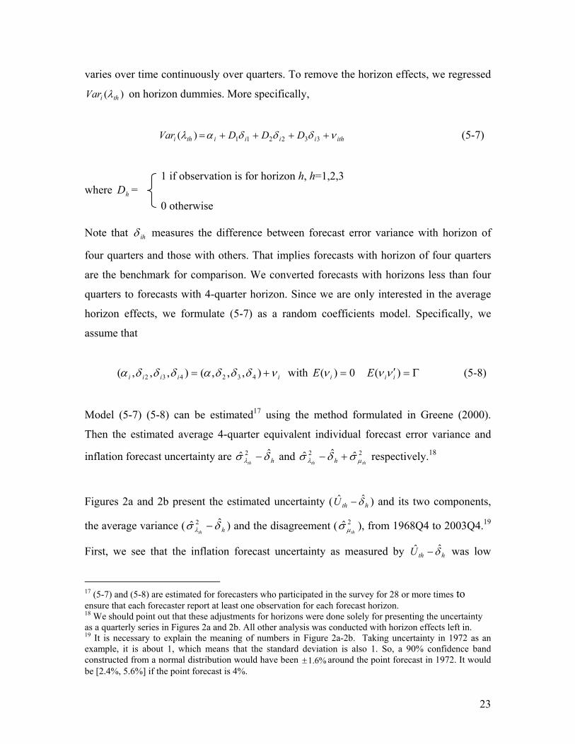
varies over time continuously over quarters. To remove the horizon effects, we regressed
)( thiVar λ on horizon dummies. More specifically,
Var ithiiiithi DDD νδδδαλ ++++= 332211)( (5-7)
1 if observation is for horizon h, h=1,2,3 where = hD 0 otherwise Note that ihδ measures the difference between forecast error variance with horizon of
four quarters and those with others. That implies forecasts with horizon of four quarters
are the benchmark for comparison. We converted forecasts with horizons less than four
quarters to forecasts with 4-quarter horizon. Since we are only interested in the average
horizon effects, we formulate (5-7) as a random coefficients model. Specifically, we
assume that
iiiii νδδδαδδδα += ),,,(),,,( 432432 with 0)( =iE ν Γ=′)( iiE νν (5-8)
Model (5-7) (5-8) can be estimated17 using the method formulated in Greene (2000).
Then the estimated average 4-quarter equivalent individual forecast error variance and
inflation forecast uncertainty are and respectively.hthδσ λˆˆ 2 − 22 ˆˆˆ
thth h µλ σδσ +− 18
Figures 2a and 2b present the estimated uncertainty (U ) and its two components,
the average variance ( ) and the disagreement ( ), from 1968Q4 to 2003Q4.
hth δ̂ˆ −
2ˆthµσhth
δσ λˆˆ 2 − 19
First, we see that the inflation forecast uncertainty as measured by U was low hth δ̂ˆ −
17 (5-7) and (5-8) are estimated for forecasters who participated in the survey for 28 or more times to ensure that each forecaster report at least one observation for each forecast horizon. 18 We should point out that these adjustments for horizons were done solely for presenting the uncertainty as a quarterly series in Figures 2a and 2b. All other analysis was conducted with horizon effects left in. 19 It is necessary to explain the meaning of numbers in Figure 2a-2b. Taking uncertainty in 1972 as an example, it is about 1, which means that the standard deviation is also 1. So, a 90% confidence band constructed from a normal distribution would have been %6.1± around the point forecast in 1972. It would be [2.4%, 5.6%] if the point forecast is 4%.
23

before 1973 and after 1992. This is consistent with previous studies. A similar pattern
persists for its two components also. This roughly confirms Friedman’s (1977) conjecture
that greater inflation uncertainty is associated with higher levels of inflation. Second, the
forecast disagreement on the average over the whole sample period is lower (0.38) than
the average of individual forecast uncertainty (0.70) over the sample period. This is
consistent with the empirical findings in previous studies such as Zarnowitz and Lambros
(1987). Third, forecast disagreement increased significantly in mid 1970s and early
1980s. In mid 1970s, the US economy was hit by the first oil shock. Such an event raises
people’s uncertainty about future change in the inflation regime. But it had interestingly
only a slight effect on the average variance of inflation, . The late 1970s and
early 1980s witnessed similar episodes when the economy is hit by the second oil shock
and a sudden change in monetary policy regime from the interest rate targeting to the
targeting of money supply.
hthδσ λˆˆ 2 −
hth δ̂−
20 Fourth, the sample variance of forecast disagreement is 0.19
over the sample period while that for the average individual forecast uncertainty is 0.11.
This is consistent with Lahiri et al. (1988)’s finding that forecast disagreement tend to be
more volatile than the average individual forecast uncertainty. Fifth, the correlation
coefficient of the overall measure of uncertainty (U ) with average variance
( ) and forecast disagreement ( ) are 0.72 and 0.85 respectively. This result
implies that forecast disagreement is a good proxy for uncertainty. Almost all studies in
this area have reached this conclusion. Finally, note from table 1 that there are significant
horizon effects. This, of course, is expected.
ˆ
hthδσ λˆˆ 2 − 2ˆ
thµσ
6. GARCH model of uncertainty In section 2, we argued that the sum of the forecast disagreement and the average
individual forecast error variance approximates the time series measure of uncertainty
fairly well. In this section, we test how well this argument is true by comparing these two
20 Evans and Wachtel (1993) find that forecast disagreement is more closely associated with regime uncertainty than the uncertainty with a given inflation structure. Since everyone knew about the change in monetary policy, the abrupt shift in disagreement in the early 80s had to be due to different beliefs and models rather than due to different information sets, see Fulford (2002) and Kurz (2002).
24

measures empirically. The most popular time series models for estimating forecast
uncertainty are ARCH and its various extensions. In these models, the forecast
uncertainty is measured as the time varying conditional variance of innovations.21
Following Engle and Kraft (1983), we model quarterly inflation tπ as an AR(4) process
tttttt επβπβπβπββπ +++++= −−−− 443322110 (6-1)
To test for the presence of conditional heteroscedasticity in the form of ARCH/GARCH
process, we estimated (6-1) by OLS on quarterly inflation data from 1955Q2 to 2004Q2
released in 2004Q3. The squared residuals are then regressed on it’s own lags up to 20.
The test statistic was significant at the significance level of 5%, suggesting that
ARCH/GARCH effect is presented.
2χ22
To capture the ARCH/GARCH effect, we tried three formulations for the conditional
variance of tε : the popular GARCH(1,1) model in which the conditional variance of
inflation is formulated as
GARCH(1,1):
(6-2) 122
11012 )|( −−− ++== ttttt hEh αεααψε
where 0α >0, 01 ≥α , 02 ≥α , 21 αα + <123 and },,{ 1111 K−−−− = tttt h επψ is the information
set at date t-1.
ARCH(4):
(6-3) 244
233
222
21101
2 )|( −−−−− ++++== ttttttt Eh εαεαεαεααψε
21 See Engle (1982, 1983), Bollerslev(1986), Nelson (1991), Glosten, Jagannathan and Runkle(1993) and surveys by Bollerslev, Chou and Kroner(1992), Bera and Higgins (1993). 22 The value of the test statistic TR was equal to 36.81. The critical value for test with 20 degree of freedom is 31.4 at significance level of 5%.
2 2χ
23 These conditions are sufficient but not necessary to ensure stationarity and nonnegativity of h . t
25
where 0α >0, 01 ≥α , 02 ≥α , ∑ . 14
1<
=iiα
GJR-GARCH(1,1):
(6-4) 2
113122
11012 )|( −−−−− +++== ttttttt DhEh εααεααψε
where 0α >0, 01 ≥α , 02 ≥α , 321 5.0 ααα ++ <1 and
<
=otherwiseif
D tt 0
01 ε
Tables 2-4 show the estimates of the three models over the same sample as above. Values
of t-statistics, log likelihood, AIC and SC reveal that GJR-GARCH(1,1) model provides
the best fit among the three models. This result is meaningful since it is well known that
an unpredicted fall in inflation produces less uncertainty than an unpredicted rise in
inflation. (Giordani and Soderlind (2003)). One explanation may be that during a period
of unexpected high inflation, people are uncertain about whether or not the monetary
authorities will adopt a disinflationary policy at the potential cost of higher
unemployment or lower growth rate of output. However, if there is unexpected low
inflation, people believe that the monetary authorities will seek to maintain the low
inflation, so inflation forecast uncertainty would be low. Actually, Ball (1992) use this
argument to explain why higher inflation leads to higher inflation uncertainty.
To make the time series results comparable to the survey measure, we estimated the
model with real-time macro data available from the Federal Reserve Bank of
Philadelphia.24 This data set includes information as they existed in the middle of each
quarter from November 1965 to the present. For each vintage date, the observations are
identical to those one would have observed at that time. To estimate our models, we 24 A description of this data set can be found in Croushore and Stark(2001).
26

make use of only the data for Output Price Index.25 (It was first GNP IPD, then GDP IPD
and finally Chain-weighted price index for real GDP since 1996, see section 4 for detail
discussion). The quarterly inflation rate is defined as log difference of quarterly price
index. Specifically,
))ln()(ln(*100 1−−= ttt ppπ
where denote the price level at date t. tp
The estimation and forecast procedure is as follows. First, the above models are estimated
using the quarterly inflation data available at a particular point of time starting from
1955Q1 and ending at the last quarter before the forecasting date. This construction is
intended to reproduce the information sets of forecasters in real time. Then the estimated
model is used to forecast the inflation forecast uncertainty. Since the survey measure
reports uncertainty associated with the forecast of annual inflation rate in the target year
made in different quarters before the end of that year, we cannot just compare the
conditional variance of quarterly inflation forecasts with the survey measure directly.
Previous studies have not been sufficiently clear about this important issue. Based on the
models for quarterly inflation, however, we could derive a measure of forecast
uncertainty comparable to the survey measure. For that purpose, we should first make
some changes to the previous notations.
Let tπ denotes annual inflation rate for year t, it ,π denotes quarterly inflation rate in the ith
quarter of year t, and denotes the price index for the iitp ,th quarter of year t. Consider the
25 The data is seasonally adjusted. For the vintage of 1996Q1, the observation for 1995Q4 is missing because of a delay in the release of statistical data caused by the federal government shutdown. For most vintages, the data start from 1947Q1. For some vintages, data may start at a different date. So, the number of observations for estimation varies across vintages not only because more observations are included over time, but also because the changes of starting date. But this only occurs for 1992Q1-1992Q4, 1999Q4-2000Q1 (starting date is 1959Q1) and 1996Q1-1997Q2 (starting date is 1959Q3) with a total of 12 among 141 vintages.
27

forecast for annual inflation rate in year t made in the first quarter of that year.26 By
definition, the annual inflation rate in year t can be expressed as the sum of quarterly
inflation rate in each quarter of that year.
1,2,3,4,4,11,1,2,
2,3,3,4,4,14,
))ln()ln()ln()ln()ln()ln()ln()(ln(*100))ln()(ln(*100
tttttttt
ttttttt
pppppppppp
πππππ
+++=−+−+
−+−=−=
−
− (6-5)
The forecast for tπ in the first quarter of that year is as follows:
(6-6) f
tf
tf
tf
ttf
tf
tf
t
ft
ft
ft
ftt
ft
ft
pppp
pppppp
1,2,3,4,4,11,1,2,
2,3,3,4,4,14,
))ln()ln()ln()ln(
)ln()ln()ln()(ln(*100))ln()(ln(*100
ππππ
π
+++=−+−+
−+−=−=
−
−
where fX denotes the forecast for the variable X made in the first quarter27 of the year
considered. So, the forecast horizon varies for predicting different quarterly inflation
rates. For example, the forecast horizon is 1/2 quarter for forecasting quarterly inflation in
the first quarter but 31/2 quarters for forecasting quarterly inflation in the fourth quarter.
The error with annual inflation forecast made in the first quarter of year t is the difference
between tπ and . ftπ
1,2,3,4,1,2,3,4,1,2,3,4, )()( tttt
ft
ft
ft
fttttt
fttt eeeee +++=+++−+++=−= ππππππππππ
(6-7)
where is the error of forecasting the iite ,th quarterly inflation of year t made in the first
quarter of the same year. As before, the quarterly inflation is modeled as AR(4). So, the
forecast for quarterly inflation rate of the fourth quarter of year t is
4,4,141,32,23,104, tttttt επβπβπβπββπ +++++= − (6-8)
26 This forecast actually has a forecast horizon of 31/2 quarters because forecasts are made at the middle of each quarter. As pointed out before, we refer to this forecast horizon as 3 quarters. 27 With real time data, it is around February 15th.
28
where 4,tε is the innovation in the fourth quarter of year t which is assumed to be
normally distributed with zero mean and a time varying conditional variance. Note that
(6-9) 4,141,32,23,104, −++++= t
ft
ft
ft
ft πβπβπβπββπ
where all forecasts are made in the first quarter of year t. Note that 4,1−tπ is known to
forecasters at that time. Based on above assumptions, we have
(6-10) 4,1,32,23,14,4,4, tttt
fttt eeee εβββππ +++=−=
Similarly, we have
(6-11) 3,1,22,13,3,3, ttt
fttt eee εββππ ++=−=
(6-12) 2,1,12,2,2, tt
fttt ee εβππ +=−=
(6-13) 1,1,1,1, t
fttte εππ =−=
By successive substitution, we have
(6-14) ∑=
+−−=i
jjitjit be
11,1, ε
where b 4411 −− ++= jjj bb ββ K , 10 =b and 0=jb for j<0.
So, the forecast uncertainty conditional on information set in the first quarter of year t is
)|()()|var()|var( 1,2,
4
1
4
0
21,1,2,3,4,1,3 tkt
k
k
jjtttttttt EbeeeeeW ψεψψ ∑ ∑
=
−
=
=+++== (6-15)
29
where 1,tψ denotes the information set in the first quarter of year t. 28 denotes the
forecast uncertainty for annual inflation rate in year t with horizon of h quarters. It is
comparable to U , the survey forecast uncertainty for annual inflation in year t with
horizon of h quarters. W with horizon other than three quarters can be derived similarly.
thW
thˆ
th
Figures 3a-3d compare the survey forecast uncertaintyUthˆ 29 with time series uncertainty
for different forecast horizons.thW 30 The time profiles and the levels are quite similar
after late 1980s. The correlations between these two series are very high after 1984 (for
all forecast horizons, the correlation coefficients are above 0.8). During this period, the
inflation rate is relatively low and stable. However, the correlation coefficients are quite
low before 1984, see table 7. This period is notable for high and volatile inflation. It
seems that the two measures give similar results when the inflation process is stable. On
the other hand, they diverge when there are structural breaks in the inflation process. This
is understandable since ARCH-type models assume that the regime for inflation and
inflation uncertainty is invariant over time while survey forecasters surely try to
anticipate structural breaks when they make forecasts.31 Although these two measures
have very low correlation in the earlier period, both of them were sensitive to the effects
of the first oil shock in 1973-74, and the second oil shock and the change in the monetary
rule in 1979-80 and 1981-82 respectively. During these periods, both measures reported
big surges. For the survey measure, by looking at Figure 2b, we find that the increase is
mostly due to the increase in the forecast disagreement. This again justifies the inclusion
of the forecast disagreement into inflation uncertainty. As Kurz (2002) has argued, when 28 Baillie and Bollerslev (1992) derived the formula for calculating for GARCH models. Similar formula for ARCH(4) and GJR-GARCH(1,1) can be found in Engle and Kraft (1983) and Blair, Poon and Taylor (2001) respectively.
)|( 1,2, tktE ψε
29 As noted before, we keep horizon effects when we compare survey measure with time series measure. 30 Time series measures of uncertainty in Figure 3a-3d is estimated and forecasted with GARCH(1,1) model. Although GJR-GARCH(1,1) model has a better fit to the most recent data as found in table 4, The profile of uncertainty over time are quite similar for these two models. For comparison with models in later part of the paper, we report the results from GARCH(1,1) model rather than GJR-GARCH(1,1) model. 31 With a Markov switching model, Evans and Wachtel (1993) estimated the regime uncertainty. According to their finding, regime uncertainty was low and stable after 1984 but high and volatile during 1968 to 1983. Although they use in sample forecast based on revised data, their finding shows that the divergence between survey measures and ARCH-type measures is due to the omission of regime uncertainty from the latter.
30
important policies are enacted, heterogeneity in beliefs creates disagreement in forecasts
that in turn contributes to the overall economic uncertainty.
To better understand the divergence between the survey measure and time series
measures, we examined the point forecasts produced by the SPF data32 and GARCH(1,1).
Figure 4a shows the point forecasts estimated by these two methods. It is obvious that
before 1984, the point forecasts estimated by the two methods are much more different
than those after 1984. On average, the sum of absolute value of difference between these
two methods is 100% larger before 1984 than after 1984. Figure 4b shows the absolute
forecast errors (forecast – actual) from these two methods. It is very obvious that from
mid 1970s to early 1980s, the GARCH point forecasts missed the actual inflation rates
substantially. The average absolute forecast errors for the AR (4) model is 1.21 during
1968-1983 (1.41 during 1973-1983) but only 0.39 during 1984-2003.33 The same for the
survey measure is 1.0 during 1968-1983 (1.11 during 1973-1983) and 0.51 during 1984-
2003. It seems that when there are structural breaks, the survey measure does better than
the time series models in forecasting inflation while during a period of low and stable
inflation, the latter does better. Since uncertainties based on ARCH-type models are
functions of forecast errors, it is not surprising to find that ARCH-type uncertainties are
bigger than the survey measure during mid 1970s and early 1980s as revealed in Figures
3a-3d. This may also explain why the survey measure of uncertainty is bigger than
ARCH-type uncertainties from mid 1980s to early 1990s for two and one quarter-ahead
forecasts.
Another undesirable feature of Figures 3a-3d is that the GARCH(1,1) measure has big
spikes in 1975 and 1976. This problem is especially serious for four-quarter ahead
forecasts. This may be due to the interaction between forecast errors and model
parameters. Notice that due to the effect of the first oil shock, GARCH(1,1) reports big
forecast errors in 1974 and 1975. Actually the two largest forecast errors for the whole
32 Consensus forecast of our sample of regular forecasters who participated at least 12 surveys. 33 The quarters for which the survey measure is missing are not included when calculating the average of absolute forecast errors for GARCH(1,1).
31

sample period occurred in these two years.34 Consequently, as a result of the GARCH
specification big forecast errors will show up as big forecast uncertainty in the following
years. That is why we have big forecast uncertainty in 1975 and 1976. One simple way to
correct this problem is just to dummy out the several quarters that have large forecast
errors. Actually, just dummying out the first and second quarters of 1975 will reduce the
spike in 1976 significantly. But this is only an ex post solution. Another explanation for
the spikes in 1975 and 1976 is that GARCH(1,1) exaggerates people’s responses to past
forecast errors. Considering this, we modified the standard GARCH(1,1) model by
formulating the conditional variance as a function of lagged conditional variance and
absolute forecast error (instead of squared forecast error).35 This method worked very
well to reduce the spikes in 1975 and 1976, especially for long horizon forecast
uncertainty. Figures 5a-5d report forecast uncertainty estimated with this modified
GARCH(1,1) model and it is obvious that the big spike in 1976 is reduced by more than
50% for four-quarter ahead forecasts. We also examined the correlation between the
survey measure and the measure based on this modified GARCH(1,1). Although it is still
much smaller during 1968-1983 than during 1984-2003, there is significant improvement
from standard GARCH(1,1), especially for the earlier period. Actually, as showed in
table 7, this model performs better than other models in the sense of reproducing the
survey measure.
Above analysis implies that a time series model that takes account of structural breaks
may match the survey measure better if the structural breaks are correctly specified. One
possible candidate is a model proposed by Evans (1991)36, in which the parameters in the
mean equation of the ARCH models are allowed to vary over time. Evans proposes three
measures of inflation forecast uncertainty, one of which is the sum of conditional
variance of innovation to inflation process and the parameter uncertainty. To see if this
34 Four-quarter ahead forecast for annual inflation in 1974 and three-quarter ahead forecast for annual inflation in 1975. 35 Taylor (1986) and Schwert (1989a, b) modeled conditional standard deviation as a distributed lag of absolute residuals. However, we found that their models could not reduce the spikes in 1975 and 1976. 36 As pointed out by Evans and Wachtel (1993), this model still fails to account for the effect of anticipated future shifts in inflation regime. They suggest a Markov switching model to explain the structural break in inflation process caused by changing regimes. One direction for future research is to generalize their model to multi-period real time forecasts.
32
formulation helps to match the survey and times series measures of inflation forecast
uncertainty, we estimated the model and obtained forecasts using real time data
recursively. Specifically, the model can be written as:
111 +++ += tttt x εβπ ),0(~ 11 ++ tt hNε (6-16)
and ],,,,1[ 4321 −−−−= tttttx ππππ , 11 ++ += ttt Vββ , V ),0(~1 QNt+
where V is a vector of normally distributed shocks to the parameter vector1+t 1+tβ with a
homoskedastic diagonal covariance matrix Q . For the theoretical and empirical
arguments for the random walk formulation, see Evans (1991) and Engle and Watson
(1985). This model can be written in state space form and estimated with the Kalman
Filter.
Observation equation: where ( ) 11
11 1 +
+
++ +
= t
t
ttt x ω
εβ
π 01 =+tω
State equation:
+
=
+
+
+
+
1
1
1
1
000
t
t
t
t
t
t VIεε
βεβ
The above model is actually a special case of the unobserved component time series
model with ARCH disturbances discussed in Harvey, Ruiz and Sentana (1992). As
pointed out by these authors, with time varying parameters, past forecast errors and
conditional variances are no longer in the information sets of forecasters and must be
inferred from the estimation of the state. They suggest a way to deal with this problem.
Following their method, we estimated the above model using real time quarterly inflation
data recursively.37 The result is shown in Figure 6 for current quarter forecasts. We find
that the estimated inflation forecast uncertainty from a time varying parameter GARCH
37 Kim and Nelson (1998) provide a GAUSS program for estimating this model. We adapt their program to get one-period-ahead forecasts. We want to express our thanks to them.
33

model is smaller than that estimated from the ordinary GARCH model during the mid
1970s. This result suggests that the divergence between time series measures and survey
measures may be resolved to a great extent by generalizing the time series models that
take into account explicitly the structural breaks and parameter drift.
7. Inflation Uncertainty using VAR-ARCH models
Univariate ARCH model and its extensions formulate inflation as a function only of its
own past values. This assumption ignores the interactions between inflation and other
variables that can be used to forecast inflation. However, as Stock and Watson (1999)
have demonstrated, some macroeconomic variables can help improve inflation forecast.
Among these variables, they find that inflation forecasts produced by the Phillips curve
generally have been more accurate than forecasts based on other macroeconomic
variables, such as interest rates, money supply and commodity prices. In this section, we
investigate if other macroeconomic variables help to match the survey measure and time
series measures of inflation forecast uncertainty. Considering the availability of real time
data, we will use the traditional Phillips curve based on unemployment.38 The forecasting
model of inflation then becomes
tttttttttt uuuu εδδδδπβπβπβπββπ +++++++++= −−−−−−−− 44332211443322110 (7-1)
where, tπ , and their lags are quarterly data on inflation and unemployment rates. To
test for the presence of conditional heteroscedasticity in the form of ARCH/GARCH
process, we estimate (7-1) by OLS over the sample period from 1955Q2 to 2004Q2
released in 2004Q3. The squared residuals were then regressed on it’s own lags up to 20.
The test found a significant ARCH/GARCH effect at the 1% level.
tu
2χ 39 One problem
with forecasting inflation by (7-1) is that we need to first forecast unemployment rate 38 This is the only variable available in real time data set at the Federal Reserve bank of Philadelphia web site as a measure of output gap. 39 The value of test statistic TR was 38.52. The critical value for test with 20 degree of freedom is 31.4 at significance level 1%.
2 2χ
34
when the forecast horizon is more than one period. This problem can be solved by
modeling unemployment also as an AR(4) process:
tttttt uuuuu υδδδδδ +++++= −−−− 443322110 (7-2)
Putting (7-1) and (7-2) together, we model inflation and unemployment as VAR-
(G)ARCH processes.
(7-3)
+
++
+
=
−
−
−
−
t
t
t
t
t
t
t
t
uuu υεπ
γδβπ
γδβ
γβπ
4
4
4
44
1
1
1
11
0
0
00L
or compactly tttt ZAZAAZ µ++++= −− 44110 L , where , .
Innovations in the inflation equation are assumed to have a time varying conditional
variance. Specifically, we assume
=
t
tt u
Zπ
=
t
tt υ
εµ
0)|( 1 =−ttE ψµ and ,
==− 2
2
1 )|var(υυευ
υευ
σσσρσσρσ
ψµt
ttttt H
where , and ),,,()|( 2111
22 KK −−− == ttttt hE σεψεσ
tttt
)()|( 21
22ttt EE υψυσυ == −
tE σσρσψυε υευευ ==− )| 1( .
Following Bollerslev(1990), we assume constant conditional correlation coefficient to
simplify ML estimation. Assuming conditional normality, the model can be estimated as
described in that paper. Tables 5 and 6 show the estimates of VAR-ARCH(1) and VAR-
GARCH(1,1) over the same sample as before.
As in the previous section, if the target variable is annual inflation rate forecasted at
different horizons, the forecast error is the sum of corresponding forecast errors for the
quarterly variables. Consider the forecast made in the first quarter of year t. The forecast
35

errors for the vector of quarterly inflation and quarterly unemployment rate in the four
quarters of year t are 1,1, tte µ= , 2,1,12, ttt eAe µ+= , 3,1,22,13, tttt eAeAe µ++= and
4,1 t,32,23,14, tttt eAeAeAe µ+++= , where denotes the value of itX , X in the ith quarter of
year t.
By successive substitution, we have
(7-4) ∑=
+−−=i
jjitjit Be
11,1, µ
where 4411 −− ++= jjj BABAB K , IB =0 , 0=jB for j<0.
After some tedious algebra, it can be shown that the forecast error for quarterly inflation
in the ith quarter of year t is
(7-5) ∑∑=
+−−=
+−− +=i
jjitj
i
jjitjit be
11,1
11,1, υλεπ
where b is defined as in (6-14) and j ∑=
−=3
0kkjkj bdλ
4411 −− ++= kkk ccd δδ K with 00 =d
4411 −− ++= jjj ccc γγ K with 10 =c and 0=jc for j<0
So, the forecast uncertainty of annual inflation conditional on the information set in the
first quarter of year t is40
40 Hlouskova, Schmidheiny and Wagner (2004) derive the general formula for the multi-step minimum mean squared error (MSE) prediction of the conditional means, variances and covariances for multivariate GARCH models with an application in portfolio management.
36

)|()|()()(2
)|()()|()(
)|var()|var(
1,2,1,
2,
4
0
3
1
4
0
1,2,
3
1
4
0
21,
2,
4
1
4
0
2
1,1,2,3,4,1,3
tkttkt
k
jj
k
k
jj
tktk
k
jjtkt
k
k
jj
tttttttt
EEb
EEb
eeeeeW
ψυψελρ
ψυλψε
ψψ
ευ
πππππ
∑∑ ∑
∑ ∑∑ ∑−
==
−
=
=
−
==
−
=
+
+=
+++==
(7-6)
We could derive the equation for calculating forecast uncertainty for other forecast
horizons similarly.
Table 7 shows the simple correlation of the survey measure with different time series
measures. Some interesting conclusions may be drawn from this table. First, on average
GARCH models simulate the survey measure better than ARCH models. The average
correlations over different forecast horizons are 0.354 and 0.322 for VAR-ARCH(1) and
ARCH(4) respectively, much lower than the correlations for corresponding VAR-
GARCH(1,1) and GARCH(1,1) models, which were 0.465 and 0.447 respectively. It
confirms the finding in the literature that changes in the conditional variance of inflation
persist over time. Actually, one motivation of developing GARCH model is to provide a
better formulation to capture this feature of inflation data (Bellerslev(1986)). Second,
univariate models perform as well as bivariate models in simulating the survey measure
of uncertainty. This may be quite surprising at first glance since it is well documented
that the Phillips curve provides a better point forecast of inflation than autoregressive
models of inflation. Ericsson (2003) discusses various determinants of forecast
uncertainty. He points out that forecast uncertainty depends upon the variable being
forecast, the type of model used for forecasting, the economic process actually
determining the variable being forecast, the information available, and the forecast
horizon. He also differentiates between actual forecast uncertainty and anticipated
forecast uncertainty, which is model dependent. In our problem, the difference between
forecast uncertainty from univariate models and that from multivariate models lies only
in the difference in model specification since they have the same target variable, same
data generating process, same information set and same forecast horizon. As explained by
Ericsson, it is not surprising that different models will produce different anticipated
forecast uncertainty. Third, models that allow for asymmetric effects of positive and
37

negative innovations came closer to the survey measure better than models that do not.
Actually, among the six models we report, GJR-GARCH(1,1) has the second highest
average correlation with the survey measure of uncertainty. Fourth, our modified
GARCH(1,1) model is the best in terms of correlation with the survey measure. As
discussed in section 6, this is because it modifies the GARCH specification by replacing
squared past errors with absolute errors. Finally, for all models, the correlation of
uncertainty of the two approaches is quite high for the period 1984-2003, a period with
low and stable inflation, but low for the period 1969-1983, a period notable for high and
unstable inflation. Actually, the relative performance of different models in simulating
the survey measure depends on how well it can simulate the survey measure during 1968-
1983. For example, the correlation with the survey measure is relatively high for GJR-
GARCH(1,1) and modified GARCH(1,1) in this period. As discussed in section 5, our
empirical estimate of the sum of the forecast disagreement and the average individual
forecast uncertainty indirectly captures model uncertainty by incorporating the forecast
disagreement. But the time series models discussed in this paper is based on a single
model to produce forecast uncertainty for all periods. This may explain the big
divergence of these two types of measures during periods with high model uncertainty.
8. Conclusions
In this paper, we develop a theoretical model to study the relationship between different
measures of inflation forecast uncertainty based on survey data and aggregate time series
models. We found that the sum of the average variance of the individual densities and the
disagreement slightly underestimates forecast uncertainty based on aggregate time series
data, and this underestimation is a function of the ratio of the variance of aggregate
shocks to that of the idiosyncratic shocks. Given the existing empirical estimates of the
ratio, we expect the underestimation to be minimal.
Even though the sum of the average variance and the disagreement is simply the variance
of the average density, we cannot directly use the variance of the aggregate distribution to
measure the aggregate forecast uncertainty due to grouping data problems, and
38
compositional effects in the panel. In this paper we lay out a tedious procedure to extract
the conceptually correct measure of aggregate uncertainty from the panel of density
forecasts.
The SPF density forecast data have an accordion structure where each respondent
forecasts year-over-year inflation rate every quarter in the current year. In order to
compare the forecast uncertainty from the surveys with those from the quarterly time
series data at various horizons, we developed the appropriate multi-period forecast
variance formulas for multivatiate ARCH-type models. During normal times (1984-
2002), the survey uncertainty and the ARCH-based time series uncertainty were
remarkably similar in their average values, correlations and temporal movements.
Another finding of our analysis is that the univariate asymmetric GARCH model did as
well as the bivariate GARCH model with Phillips Curve.
During periods of rapid structural change (like the oil crises or Fed’s new operating
policies of early 80’s), we found that the two approaches could yield quite different
estimates of uncertainty. Since these periods are characterized by larger forecast errors in
time series models than in survey data, the time series uncertainty shoots up much more
than the survey measure. During periods of rapid change, it is the disagreement
component of uncertainty and not the average variance of the densities that responds, but
not by as much as the time series uncertainty. We found a simple way to make the time
series estimates robust to exceptionally large forecast errors; the trick is to model the
conditional variance not as a function of squared forecast errors but as a function of its
absolute value.
Another fruitful approach will be to model the time series ARCH model as a time varying
parameter model. We found that this approach also helps in robustifying ARCH
uncertainty estimates to abrupt structural breaks. Even then, the survey uncertainty tends
to respond more prospectively than time series models. Thus, during periods of structural
breaks and regime change, survey measure of uncertainty can be very dependable, and
should be monitored carefully in conjunction with the time series measures. This reminds
39
us of the sentiment Manski (2004) expressed when he wrote, “Economists have long been
hostile to subjective data. Caution is prudent but hostility is not warranted.” Our analysis
shows that by carefully utilizing the SPF density forecasts data, we can gather substantial
knowledge about the temporal pattern of aggregate uncertainty of inflation forecasts,
particularly when time series models could be failing. There remains much unexploited
potential in the use of this subjective database.
40

References Baillie, R.T. and T. Bollerslev (1992), “Prediction in dynamic models with time-
dependent conditional variance”, Journal of Econometrics, 52, 91-113.
Ball, L. (1992), “Why does high inflation raise inflation uncertainty?” Journal of
Monetary Economics, 371-388.
Ball, L. and N.G. Mankiw (1995), “Relative-price changes as aggregate supply shocks”,
Quarterly Journal of Economics, 110, 161-193.
Batchelor, R. and P. Dua (1993), “Survey vs. ARCH measures of uncertainty”, Oxford
Bulletin of Economics and Statistics, 55, 341-353.
Batchelor, R. and P. Dua (1995), “Forecaster diversity and the benefits of combining
forecasts”, Management Science, 41, 68-75.
Batchelor, R. and P. Dua (1996), “Empirical measures of inflation uncertainty: a
cautionary note”, Applied Economics, 28, 333-341.
Bera, A.K. and Higgins, M.L. (1993), “ARCH models: properties, estimation and
testing”, Journal of Economic Surveys, 7, 305-362.
Blair B.J., S.H. Poon and S.J. Taylor (2001), “Forecasting S&P 100 volatility: the
incremental information content of implied volatilities and high-frequency index return”,
Journal of econometrics, 105, 5-26.
Bollerslev, T. (1986), “Generalized autoregressive conditional heteroscedasticity”,
Journal of Econometrics, 31, 307-327.
41

Bollerslev, T. (1990), “Modeling the coherence in short-run nominal exchange rates: A
multivariate generalized ARCH model”, Review of Economics and Statistics, 72, 498-
505.
Bollerslev, T., Chou, R.Y. and K.P. Kroner (1992), “ARCH modeling in finance: a
review of theory and empirical evidence”, Journal of Econometrics, 52, 5-59.
Bomberger, W.A. (1996), “Disagreement as a measure of uncertainty”, Journal of
Money, Credit and Banking, 28, 381-392.
Carroll, C.D. (2003), “Macroeconomic expectations of households and professional
forecasters”, Quarterly Journal of Economics, 118, 269-298.
Christofferson, P.F., and F.X. Diebold (1997), “Optimal prediction under asymmetric
loss”, Econometric Theory, 13, 808-817.
Cogley, T., S. Morozov and T. J. Sargent (2003), “Bayesian Fan Charts for U.K.
Inflation: Forecasting and Sources of Uncertainty in an Evolving Monetary System”,
Draft, July 2003.
Croushore, D. and T. Stark (2001), “A real-time data set for macroeconomists”, Journal
of econometrics, 105, 111-130.
Cukierman, A. and P. Wachtel (1979), “Differential inflationary expectations and the
variability of the rate of inflation: theory and evidence ”, American Economic Review, 69,
595-609.
Cukierman, A. and P. Wachtel (1982), “relative price variability and nonuniform
inflationary expectations ”, Journal of Political Economy, 90, 146-157.
42

Davies, A. and K. Lahiri (1995), “A new framework for analyzing survey forecasts using
three-dimensional panel data”, Journal of Econometrics, 68, 205-227.
Davies, A. and K. Lahiri (1999), “Re-examining the rational expectations hypothesis
using panel data on multi-period forecasts” In Hsiao, C., Lahiri, K., Lee, L.F. and
Pesaran, H. (Eds.) Analysis of Panels and Limited Dependent Variable Models.
Cambridge: Cambridge University Press.
Diebold, F., A. Tay and K. Wallis (1999), “Evaluating Density Forecasts of Inflation:
The Survey of Professional Forecasters,” in R. Engle and H. White (eds.), Cointegration,
Causality, and Forecasting: A Festschrift in Honor of Clive W.J. Granger, 76-90, 1999.
Oxford: Oxford University Press.
Engle, R. (1982), “Autoregressive conditional heteroscedasticity with estimates of the
variance of United Kingdom inflation”, Econometrica, 50, 987-1008.
Engle, R. (1983), “Estimates of the variance of U.S. inflation based upon the ARCH
model”, Journal of Money, Credit and Banking, 15, 286-301.
Engle, R.F. and D. Kraft (1983), “Multiperiod forecast error variances of inflation
estimated from ARCH models”, in: A. Zellner, ed., Applied time series analysis of
economic data (Bureau of the Census, Washington, DC), 293-302.
Engle, R. F. and Watson, M.W. (1985), “The Kalman filter: applications to forecasting
and rational-expectations models” in: Truman Bewley, ed., Advances in econometrics,
Vol. I, Fifth World Congress of the Econometric Society.
Ericsson, N.R. (2003), “Forecast uncertainty in economic modeling” In understanding
economic forecasts, edited by David F. Hendry and Neil R. Ericsson, 68-92, Cambridge
and London, MIT Press.
43
Evans, M. (1991), “Discovering the link between inflation rates and inflation
uncertainty”, Journal of Money, Credit and Banking, 23, 169-184.
Evans, M. and P. Wachtel (1993), “Inflation regimes and the sources of inflation
uncertainty”, Journal of Money, Credit and Banking, 25, 475-511.
Friedman, M. (1977), “Nobel Lecture: inflation and unemployment”, The Journal of
Political Economy, 85, 451-472.
Fuhrer, J.C., (1988), “On the information content of consumer survey expectations”,
Review of Economics and Statistics, 70, No. 1, 140-144.
Fukford, S.L. (2002), “The Impact of monetary policy on the cross-sectional variance of
expectations of inflation”, Stanford University, mimeo.
Garratt, A., K. Lee, M. H. Pesaran and Y. Shin (2003), “Forecast uncertainty in
macroeconomic modelling: an application to the U.K. ecomomy”, Journal of the
American Statistical Association, 98, 829-838.
Giordani, P. and P. Söderlind (2003), “Inflation forecast uncertainty”, European
Economic Review, 47, 1037-1059.
Glosten, L., R. Jagannathan, and D. Runkle (1993), “On the relation between the
expected value and the volatility of the nominal excess return on stocks”, Journal of
Finance, 48, 1779-1801.
Greene, W.H., Econometric Analysis, 4th Edition, Prentice Hall, Upper Saddle River,
New Jersey, 2000.
Harvey A., E. Ruiz and E. Sentana (1992), “Unobserved component time series models
with ARCH disturbances”, Journal of Econometrics 52, 129-157.
44

Hlouskova J., K. Schmidheiny and M. Wagner (2004), “Multistep predictions for
multivariate GARCH models: closed form solution and the value for portfolio
management”, Draft, 2004.
Irwin, S.H., M.E. Gerlow and T.R. Liu (1994), “The forecasting performance of livestock
futures prices: a comparison of USDA expert predictions”, Journal of Futures Markets,
14, 861-875.
Kastens, T. L., T.C. Schroeder and R. Plain (1998), “Evaluation of extension and USDA
price and production forecasts”, Journal of Agricultural and Resource Economics, 23,
244-261.
Kim, C.-J. and C.R. Nelson (1998), State-Space Model with Regime-Switching: Classical
and Gibbs-sampling Approaches with Applications, MIT Press: Cambridge, MA.
Kurz, M. (2002), “Heterogeneous forecasting and Federal Reserve information”, Stanford
University, 2002, mimeo.
Kurz, M. and M. Motolese (2001), “Endogenous uncertainty and market volatility”,
Economic Theory, 17, 497-544.
Lahiri, K., and D. Ivanova (1998), "A time series and cross sectional analysis of
consumer sentiment and its components", In Social Structural Change - Consequences
for Business Cycle Surveys, (Eds. K. H. Oppenländer and G. Poser), Aldershot: Ashgate
Publishing, England, 337-362.
Lahiri, K. and C. Teigland (1987), “On the normality of probability distribution and GNP
forecasts”, International Journal of Forecasting, 3, 269-279.
45

Lahiri, K., C. Teigland and M. Zaporowski (1988), “Interest rates and the subjective
probability distribution of inflation forecasts”, Journal of Money, Credit and Banking, 20,
233-248.
Laster, D., P. Bennett and I.S. Geoum (1999), “Rational bias in macroeconomic
forecast”, The Quarterly Journal of Economics, 114, 293-318.
Levi, M. and J. Makin (1978), “Anticipated inflation and interest rates: Further
interpretation of findings on the Fisher equation”, American Economic Review, 68, 801-
812.
Lucas, R.E. (1972), “Expectations and the neutrality of money”, Journal of Economic
Theory, 4, 103-124.
Lucas, R.E. (1973), “Some international evidence on output-inflation tradeoffs”,
American Economic Review, 63, 326-334.
Makin, J. (1983), “Real interest, money surprises, anticipated inflation, and fiscal
deficits”, Review of Economics and Statistics, 65, 374-384.
Mankiw, N.G., R. Reis and J. Wolfers (2003), “Disagreement about inflation expectation”, NBER Working Paper No. w9796.
Mankiw, N.G., R. Reis (2002), “Sticky information versus sticky prices: a proposal to
replace the new Keynesian Phillips curve”, Quarterly Journal of Economics, 117, 1295-
1328.
Manski, C.F. (2004), “Measuring expectations”, Econometrica, 72, 1329-1376.
McNees, S. (1989), “Why do forecasts differ”, New England Economic Review,
Jan./Feb., 42-54.
46

Nelson, D.B. (1991), “Conditional heteroskedasticity in asset returns: a new approach”,
Econometrica, 59, 347-370.
Palm, F., and A. Zellner (1992), “To combine or not to combine? Issue of combining
forecasts”, Journal of Forecasting, 11, 687-701.
Rich, R. and J. Tracy (2003), “Modeling uncertainty: Predictive accuracy as a proxy for
predictive confidence”, Federal Reserve Bank of New York Staff Reports, No.161.
Schwert, G.W. (1989a), “Why does stock market volatility change over time”, Journal of
Finance, 44, 1115-1153.
Schwert, G.W. (1989b), “Business cycles, financial crises, and stock volatility”,
Carnegie-Rochester Conference Series on Public Policy, 39, 83-126.
Sims, C. (2002), “The role of models and probabilities in the monetary policy process”,
Brookings Papers on Economic Activity, 2002(2), 1-62.
Šmidková, K. (2003), “Methods available to monetary policy makers to deal with
uncertainty”, paper presented at the conference “Forecasting in a Central Bank”, Bank of
England, August 2003, London.
Souleles, N., (2004), “Expectations, heterogeneous forecast errors, and consumption:
micro evidence from the Michigan Consumer Sentiment Surveys”, Journal of Money,
Credit and Banking, 36, 39-72.
Stock, J. and M.W. Watson (1999), “Forecasting inflation”, Journal of Monetary
Economics, 44, 293-335.
47
Stuart, A. and J.K. Ord (1994), Kendall’s advanced theory of statistics, vol1, John Wiley
& Sons Inc.
Taylor, S. (1986), Modeling Financial Time Series. Wiley and Sons: New York, NY.
Wallis, K.F. (2004), “Combining density and interval forecasts: a modest proposal”,
Mimeo, October 2004. University of Warwick, UK.
Zarnowitz, V. and L.A. Lambros (1987), “Consensus and uncertainty in economic
prediction”, Journal of Political Economy, 95, 591-620.
Zellner, A. (1986), Bayesian estimation and prediction using asymmetric loss functions,
Journal of the American Statistical Association, 81, 446-451.
48

Table 1. Estimates of average horizon effects.
variable Coefficients Std. Error t-statistic p-value
α̂ 0.6676 0.029 23.378 0.000
3̂δ -0.0006 0.023 -0.025 0.98
2δ̂ -0.0929 0.019 -5.017 0.000
1̂δ -0.1959 0.018 -10.704 0.000
49

Table 2. GARCH(1,1) estimates.
variable Coefficient Std. Error t-statistic p-value
c 0.0510 0.0288 1.7717 0.076
1−tπ 0.4708 0.0767 6.1402 0.000
2−tπ 0.1780 0.0811 2.1947 0.028
3−tπ 0.0393 0.0826 0.4755 0.634
4−tπ 0.2301 0.0712 3.2316 0.001
Variance Equation
c 0.0018 0.0013 1.3556 0.175 2
1−tε 0.1278 0.0482 2.6536 0.008
1−th 0.8439 0.0535 15.7737 0.000
807.02 =R ; Log Likelihood=5.005; AIC=0.000; SC=0.084
Table 3. ARCH(4) estimates.
variable Coefficient Std. Error t-statistic p-value
c 0.0567 0.0374 1.5175 0.129
1−tπ 0.4372 0.0746 5.8574 0.000
2−tπ 0.2252 0.1171 1.9237 0.054
3−tπ 0.0325 0.1058 0.3069 0.759
4−tπ 0.2147 0.0762 2.8193 0.005
Variance Equation
c 0.0185 0.0067 2.7713 0.006 2
1−tε 0.2038 0.1393 1.4625 0.144
22−tε 0.1482 0.1341 1.1052 0.269
23−tε 0.1547 0.0852 1.8154 0.069
24−tε 0.2677 0.1242 2.1557 0.031
795.02 =R ; Log Likelihood=2.341; AIC=0.027; SC=0.111
50

Table 4. GJR-GARCH(1,1) estimates.
variable Coefficient Std. Error t-statistic p-value
c 0.0567 0.0273 2.0784 0.038
1−tπ 0.5018 0.0820 6.1173 0.000
2−tπ 0.1621 0.0854 1.8982 0.058
3−tπ 0.0195 0.0817 0.2383 0.812
4−tπ 0.2454 0.0690 3.5574 0.000
Variance Equation
c 0.002 0.0013 1.5954 0.111 2
1−tε 0.2127 0.0869 2.4473 0.014
1−th 0.8546 0.0746 11.4614 0.000
211 −− ttD ε -0.2127 0.0831 -2.5606 0.010
810.02 =R ; Log Likelihood=10.614; AIC=-0.058; SC=0.026
51
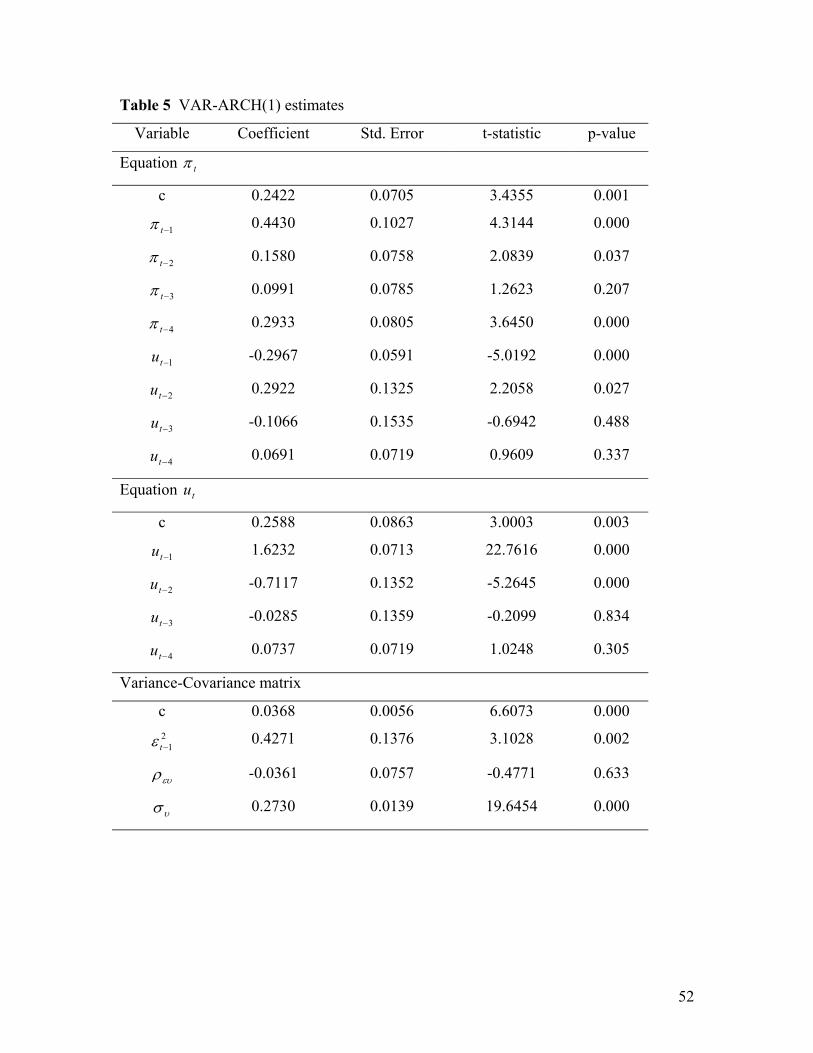
Table 5 VAR-ARCH(1) estimates
Variable Coefficient Std. Error t-statistic p-value
Equation tπ
c 0.2422 0.0705 3.4355 0.001
1−tπ 0.4430 0.1027 4.3144 0.000
2−tπ 0.1580 0.0758 2.0839 0.037
3−tπ 0.0991 0.0785 1.2623 0.207
4−tπ 0.2933 0.0805 3.6450 0.000
1−tu -0.2967 0.0591 -5.0192 0.000
2−tu 0.2922 0.1325 2.2058 0.027
3−tu -0.1066 0.1535 -0.6942 0.488
4−tu 0.0691 0.0719 0.9609 0.337
Equation u t
c 0.2588 0.0863 3.0003 0.003
1−tu 1.6232 0.0713 22.7616 0.000
2−tu -0.7117 0.1352 -5.2645 0.000
3−tu -0.0285 0.1359 -0.2099 0.834
4−tu 0.0737 0.0719 1.0248 0.305
Variance-Covariance matrix
c 0.0368 0.0056 6.6073 0.000 2
1−tε 0.4271 0.1376 3.1028 0.002
ευρ -0.0361 0.0757 -0.4771 0.633
υσ 0.2730 0.0139 19.6454 0.000
52

Table 6 VAR-GARCH(1,1) estimates
Variable Coefficient Std. Error t-statistic p-value
Equation tπ
c 0.2288 0.0660 3.4651 0.001
1−tπ 0.3888 0.0769 5.0543 0.000
2−tπ 0.2044 0.0783 2.6107 0.009
3−tπ 0.0774 0.0781 0.9913 0.322
4−tπ 0.3067 0.0698 4.3925 0.000
1−tu -0.2568 0.0599 -4.2870 0.000
2−tu 0.2245 0.1105 2.0322 0.042
3−tu 0.0222 0.1093 0.2027 0.839
4−tu -0.0291 0.0569 -0.5107 0.610
Equation u t
c 0.2585 0.0863 2.9963 0.003
1−tu 1.6219 0.0703 23.0717 0.000
2−tu -0.7100 0.1264 -5.6171 0.000
3−tu -0.0299 0.1163 -0.2569 0.797
4−tu 0.0747 0.0633 1.1802 0.238
Variance-Covariance matrix
c 0.0021 0.0017 1.2909 0.197 2
1−tε 0.1627 0.0723 2.2494 0.024
21−tσ 0.8008 0.0852 9.4013 0.000
ευρ -0.0260 0.0751 -0.3460 0.729
υσ 0.2730 0.0139 19.6461 0.000
53
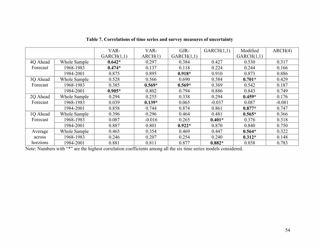
Table 7. Correlations of time series and survey measures of uncertainty
VAR-GARCH(1,1)
VAR-ARCH(1)
GJR-GARCH(1,1)
GARCH(1,1) ModifiedGARCH(1,1)
ARCH(4)
Whole Sample 0.642* 0.297 0.384 0.427 0.530 0.3171968-1983 0.474* 0.137 0.118 0.224 0.244 0.166
4Q Ahead Forecast
1984-2001 0.875 0.895 0.918* 0.910 0.873 0.886Whole Sample 0.528 0.566 0.690 0.584 0.701* 0.429
1968-1983 0.385 0.569* 0.569* 0.369 0.542 0.1873Q Ahead Forecast
1984-2001 0.905* 0.802 0.794 0.886 0.843 0.749Whole Sample 0.294 0.255 0.338 0.294 0.459* 0.176
1968-1983 0.039 0.139* 0.065 -0.037 0.087 -0.0812Q Ahead Forecast
1984-2001 0.858 0.744 0.874 0.861 0.877* 0.747 Whole Sample 0.396 0.296 0.464 0.481 0.565* 0.366
1968-1983 0.087 -0.016 0.265 0.401* 0.376 0.3181Q Ahead Forecast
1984-2001 0.887 0.801 0.922* 0.870 0.840 0.750Whole Sample 0.465 0.354 0.469 0.447 0.564* 0.322
1968-1983 0.246 0.207 0.254 0.240 0.312* 0.148 Average across
horzions 1984-2001 0.881 0.811 0.877 0.882* 0.858 0.783Note: Numbers with “*” are the highest correlation coefficients among all the six time series models considered.
54
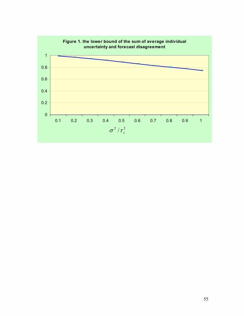
Figure 1. the lower bound of the sum of average individual uncertainty and forecast disagreement
0
0.2
0.4
0.6
0.8
1
0.1 0.2 0.3 0.4 0.5 0.6 0.7 0.8 0.9 1
22
/ zτσ
55
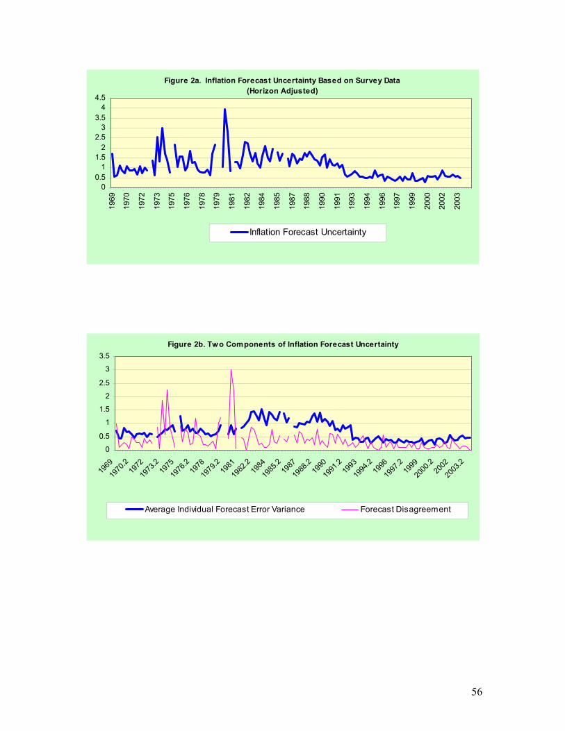
Figure 2a. Inflation Forecast Uncertainty Based on Survey Data(Horizon Adjusted)
00.5
11.5
22.5
33.5
44.5
1969
1970
1972
1973
1975
1976
1978
1979
1981
1982
1984
1985
1987
1988
1990
1991
1993
1994
1996
1997
1999
2000
2002
2003
Inflation Forecast Uncertainty
Figure 2b. Two Components of Inflation Forecast Uncertainty
0
0.5
1
1.5
2
2.5
3
3.5
1969
1970
.219
72
1973
.219
75
1976
.219
78
1979
.219
81
1982
.219
84
1985
.219
87
1988
.219
90
1991
.219
93
1994
.219
96
1997
.219
99
2000
.220
02
2003
.2
Average Individual Forecast Error Variance Forecast Disagreement
56

Figure 3a. Four-Quarter Ahead Forecast Uncertainty
0
2
4
6
8
10
12
Measure Estimated from GARCH(1,1)Measure Estimated from Survey Data
Figure 3b. Three-Quarter Ahead Forecast Uncertainty
0
1
2
3
4
5
6
Measure Estimated from GARCH(1,1)Measure Estimated from Survey Data
Figure 3c. Two-Quarter Ahead Forecast Uncertainty
0123456
Measure Esimated from GARCH(1,1)Measure Estimated from Survey Data
Figure 3d. One-Quarter Ahead Forecast Uncertainty
0
1
2
3
4
5
6
Measure Estimated from GARCH(1,1)Measure Estimated from Survey Data
57
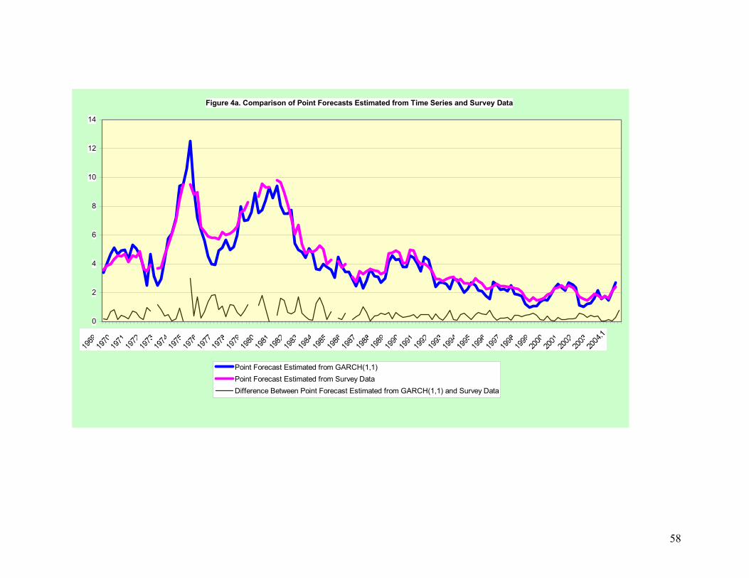
Figure 4a. Comparison of Point Forecasts Estimated from Time Series and Survey Data
0
2
4
6
8
10
12
14
Point Forecast Estimated from GARCH(1,1)Point Forecast Estimated from Survey DataDifference Between Point Forecast Estimated from GARCH(1,1) and Survey Data
58
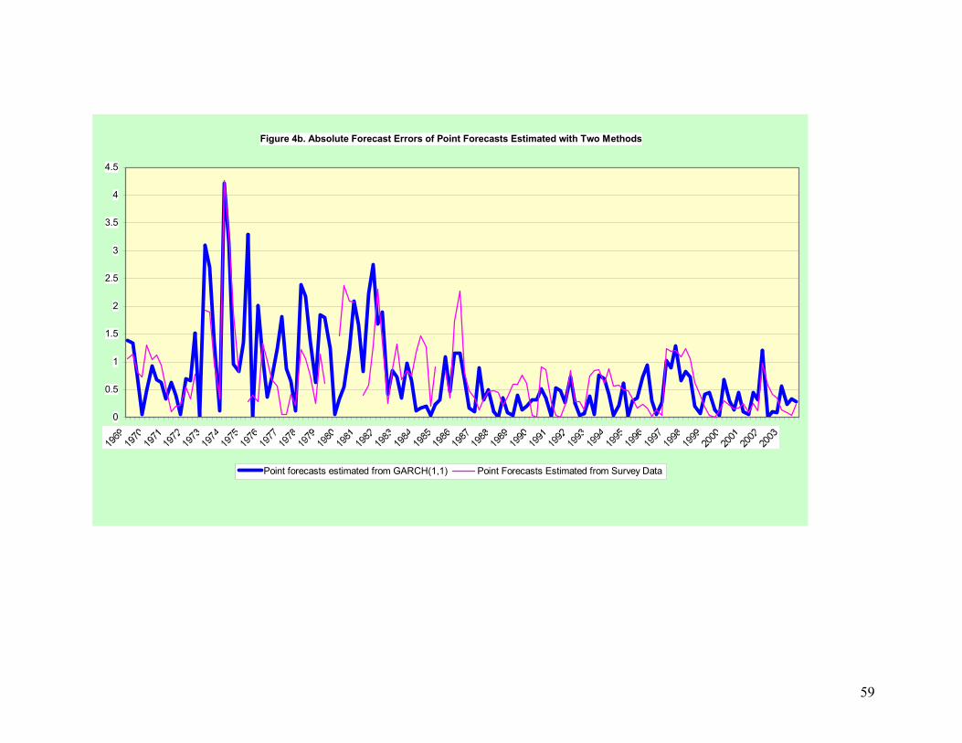
Figure 4b. Absolute Forecast Errors of Point Forecasts Estimated with Two Methods
0
0.5
1
1.5
2
2.5
3
3.5
4
4.5
Point forecasts estimated from GARCH(1,1) Point Forecasts Estimated from Survey Data
59

Figure 5a. Four-Quarter Ahead Forecast Uncertainty
01
23
45
6
Measure Estimated from Modified GARCH(1,1)Survey Measure
Figure 5b. Three-Quarter Ahead Forecast Uncertainty
0123456
Measure Estimated from Modified GARCH(1,1)Survey Measure
Figure 5c. Two-Quarter Ahead Forecast Uncertainty
0
1
2
3
4
5
6
Measure Estimated from Modified GARCH(1,1)Survey Measure
Figure 5d. One-Quarter Ahead Forecast Uncertainty
0
1
2
3
4
5
6
Measure Estimated from Modified GARCH(1,1)Survey Measure
60

Figure 6. Current Quarter Forecast Uncertainty
0
0.1
0.2
0.3
0.4
0.5
0.6
0.7
0.8
1968
1970
1972
1974
1976
1978
1980
1982
1984
1986
1988
1990
1992
1994
1996
1998
2000
2002
Measure Estimated from GARCH(1,1)Measure Estimated from GARCH(1,1) with Time-varying Parameters on the Mean Equation
61
Top Related