


Languages
Pages
Legal


Gary WeissmannUniversity of New Mexico
Application of Transition Probability Geostatistics in a
Detailed Stratigraphic Framework

ACKNOWLEDGEMENTSNational Science FoundationAmerican Chemical Society –
Petroleum Research FundUS Department of AgricultureUS Geological SurveyUniversity of California Water
Resources CenterOccidental Chemical CompanyGeological Society of America
Graham Fogg Yong ZhangEric LaBolle Steve CarleThomas Harter Karen BurowGeorge Bennett Sarah NorrisDeitz Warnke Ken VerosubJeffrey Mount Michael SingerGordon Huntington
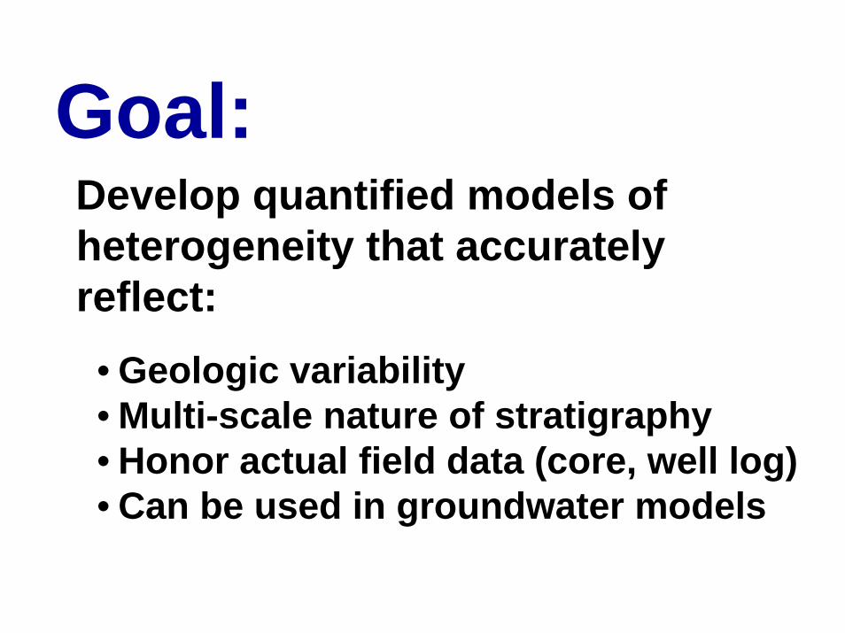
Goal:Develop quantified models of heterogeneity that accurately reflect:• Geologic variability• Multi-scale nature of stratigraphy• Honor actual field data (core, well log)• Can be used in groundwater models
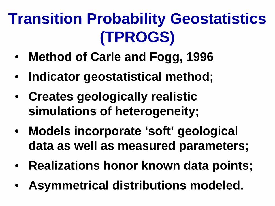
Transition Probability Geostatistics(TPROGS)
• Method of Carle and Fogg, 1996• Indicator geostatistical method;• Creates geologically realistic
simulations of heterogeneity;• Models incorporate ‘soft’ geological
data as well as measured parameters;• Realizations honor known data points;• Asymmetrical distributions modeled.
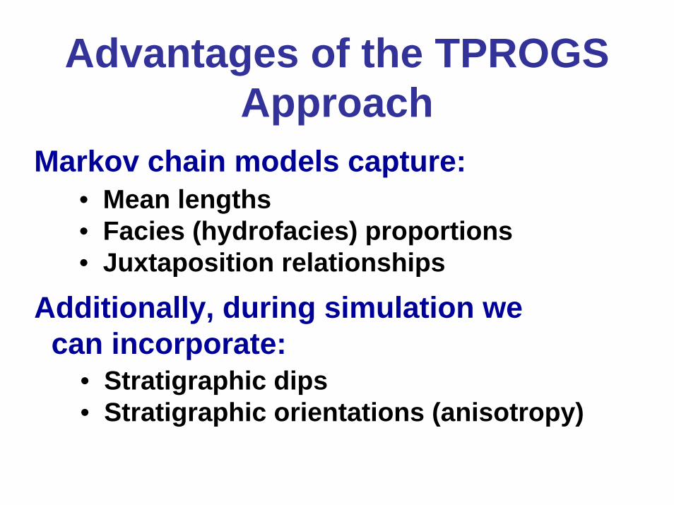
Markov chain models capture:• Mean lengths• Facies (hydrofacies) proportions• Juxtaposition relationships
Additionally, during simulation we can incorporate:
• Stratigraphic dips• Stratigraphic orientations (anisotropy)
Advantages of the TPROGS Approach

Kings River Alluvial Fan
20km1980 Landsat MSS false color from USGS NALC program.
Fresno

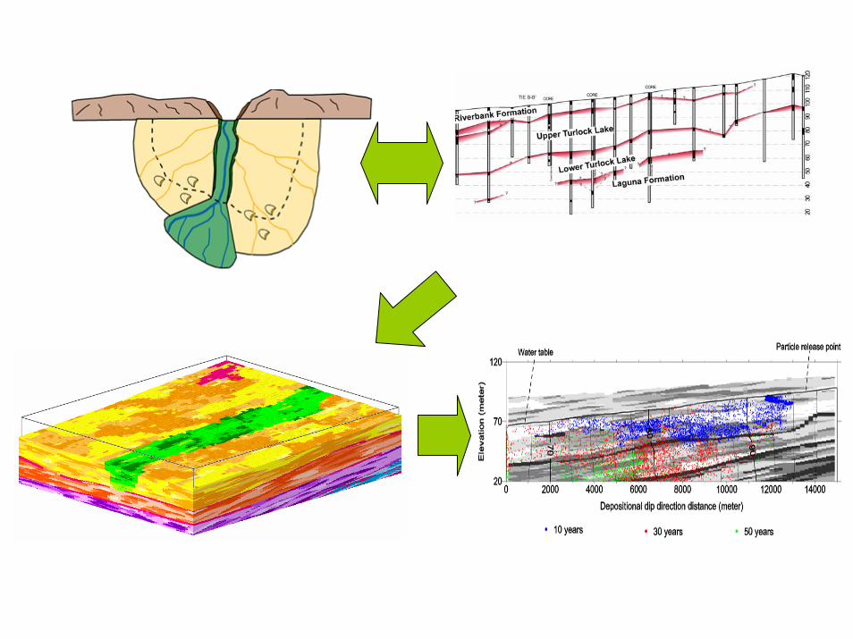
STEPS FOR MODELING1. Define and model overall stratigraphy and define ‘units’ where
local stationarity is a reasonable assumption.
2. Measure vertical transition probabilities between facies within each ‘unit’ and fit 1-D Markov chain model(s) to these measured results.
3. Measure or estimate lateral transition probabilities and estimate lateral Markov chain models for each ‘unit.’a. From well datab. From other sources (e.g., soil surveys, geological maps).
4. Simulate each ‘unit’ separately.a. Conditional Sequential Indicator Simulation.b. Simulated Quenching.
5. Combine simulation results into single realization of system.
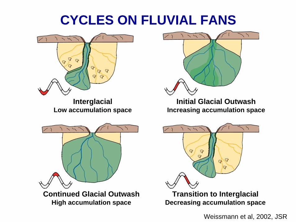
CYCLES ON FLUVIAL FANS
InterglacialLow accumulation space
Initial Glacial OutwashIncreasing accumulation space
Continued Glacial OutwashHigh accumulation space
Transition to InterglacialDecreasing accumulation space
Weissmann et al, 2002, JSR
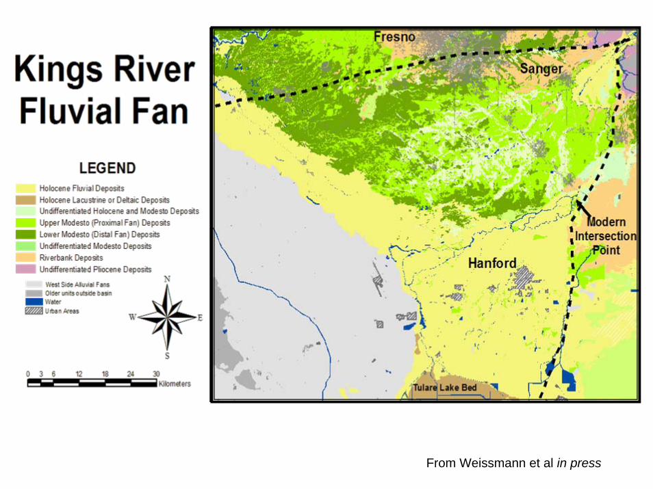
From Weissmann et al in press

Basinward Apex
Kings River Alluvial Fan – Dip Section
From Weissmann et al 2002
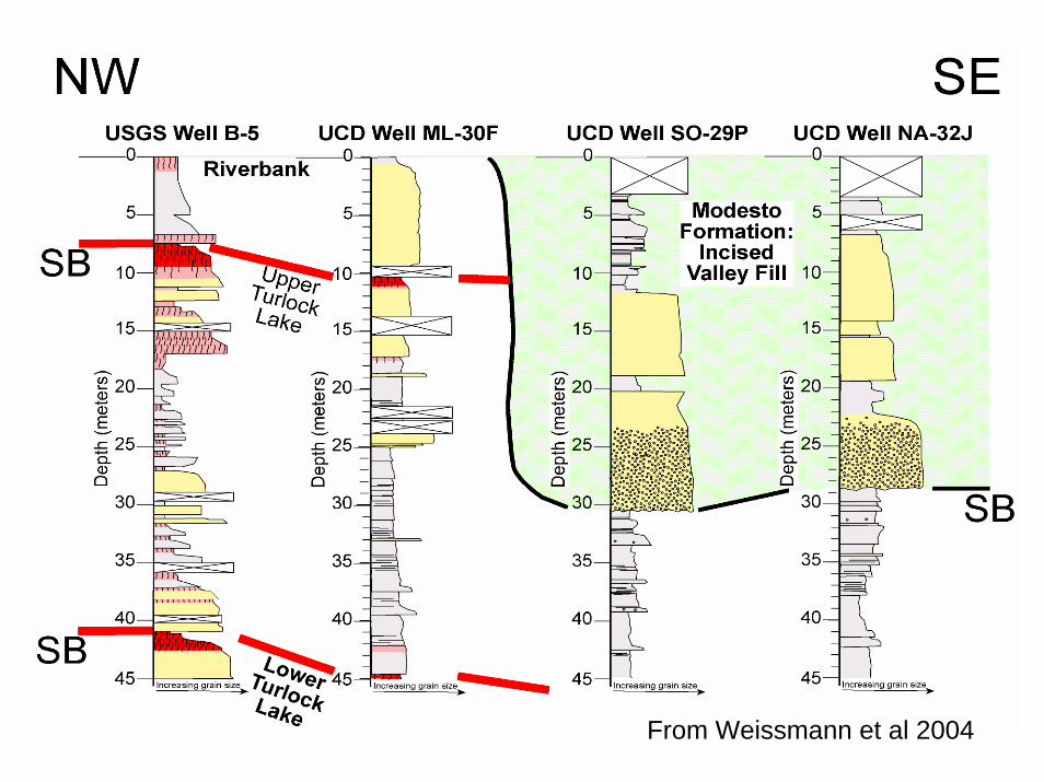
From Weissmann et al 2004
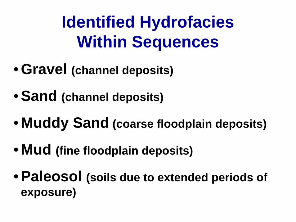
Identified Hydrofacies Within Sequences
• Gravel (channel deposits)
• Sand (channel deposits)
• Muddy Sand (coarse floodplain deposits)
• Mud (fine floodplain deposits)
• Paleosol (soils due to extended periods of exposure)

From Weissmann et al 2004

STEPS FOR MODELING1. Define and model overall stratigraphy and define ‘units’ where
local stationarity is a reasonable assumption.
2. Measure vertical transition probabilities between facies within each ‘unit’ and fit 1-D Markov chain model(s) to these measured results.
3. Measure or estimate lateral transition probabilities and estimate lateral Markov chain models for each ‘unit.’a. From well datab. From other sources (e.g., soil surveys, geological maps).
4. Simulate each ‘unit’ separately.a. Conditional Sequential Indicator Simulation.b. Simulated Quenching.
5. Combine simulation results into single realization of system.
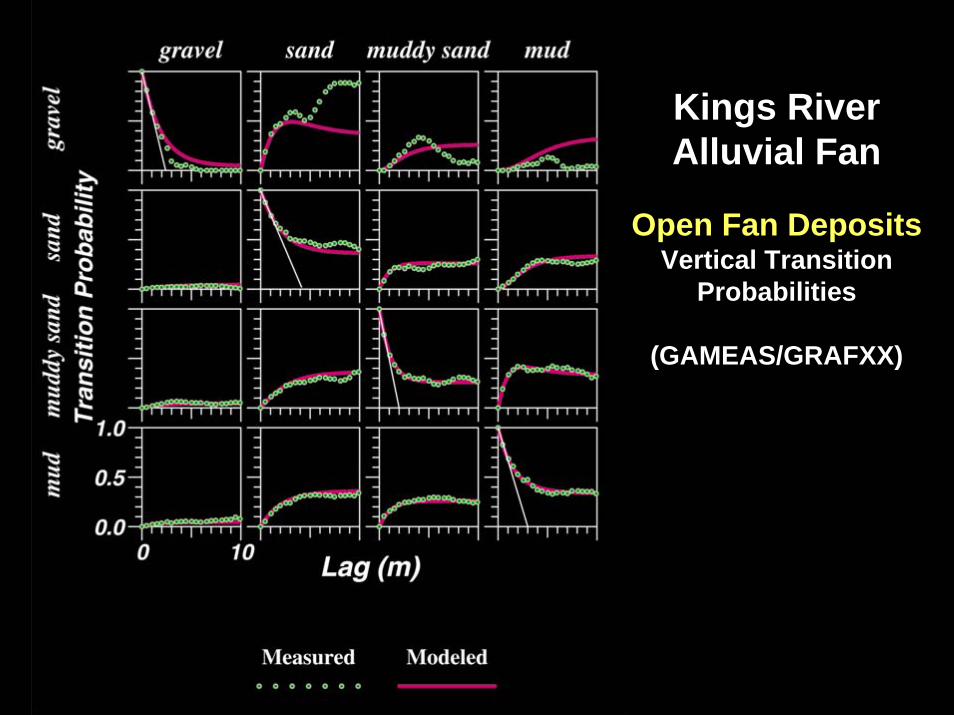
Kings River Alluvial Fan
Open Fan DepositsVertical Transition
Probabilities
(GAMEAS/GRAFXX)
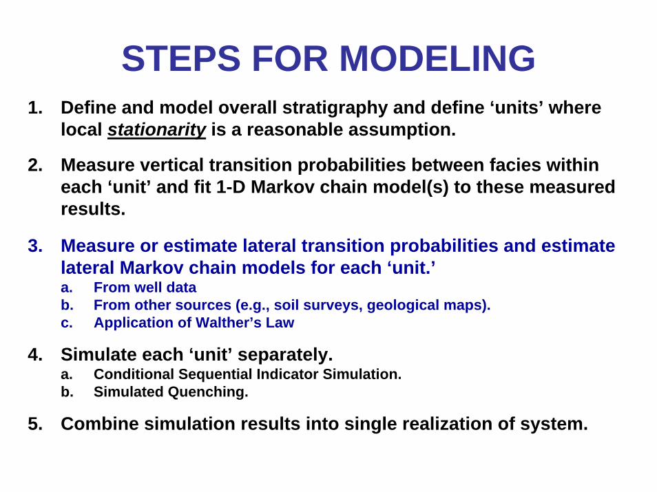
STEPS FOR MODELING1. Define and model overall stratigraphy and define ‘units’ where
local stationarity is a reasonable assumption.
2. Measure vertical transition probabilities between facies within each ‘unit’ and fit 1-D Markov chain model(s) to these measured results.
3. Measure or estimate lateral transition probabilities and estimate lateral Markov chain models for each ‘unit.’a. From well datab. From other sources (e.g., soil surveys, geological maps).c. Application of Walther’s Law
4. Simulate each ‘unit’ separately.a. Conditional Sequential Indicator Simulation.b. Simulated Quenching.
5. Combine simulation results into single realization of system.
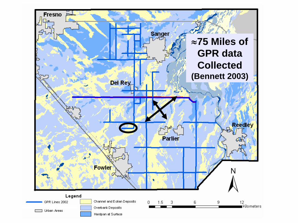
≈75 Miles of GPR data Collected
(Bennett 2003)
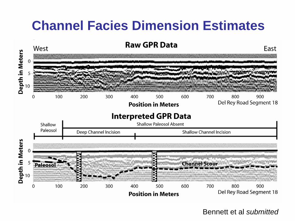
Channel Facies Dimension Estimates
Bennett et al submitted

STEPS FOR MODELING1. Define and model overall stratigraphy and define ‘units’ where
local stationarity is a reasonable assumption.
2. Measure vertical transition probabilities between facies within each ‘unit’ and fit 1-D Markov chain model(s) to these measured results.
3. Measure or estimate lateral transition probabilities and estimate lateral Markov chain models for each ‘unit.’a. From well datab. From other sources (e.g., soil surveys, geological maps).c. Application of Walther’s Law
4. Simulate each ‘unit’ separately.a. Conditional Sequential Indicator Simulation.b. Simulated Quenching.
5. Combine simulation results into single realization of system.


Realizations capture:• Contrasting character between different stratigraphic units.• Fining-upward successions (gravel up to sand up to muddy sand)• Juxtapositional tendencies (fining-outward successions)• Radial pattern of fan deposits• Dipping beds• Reasonable channel sand and floodplain fine distributions. It
“looks” geological.• And honor conditioning data points
Multiple realizations can be run to assess uncertainty.
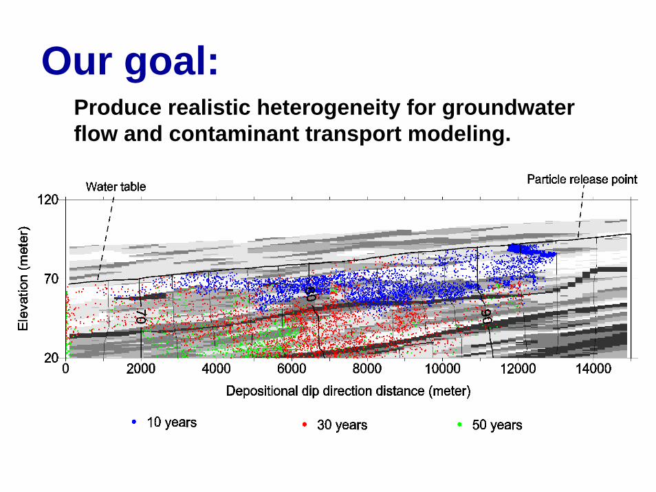
Our goal:Produce realistic heterogeneity for groundwater flow and contaminant transport modeling.
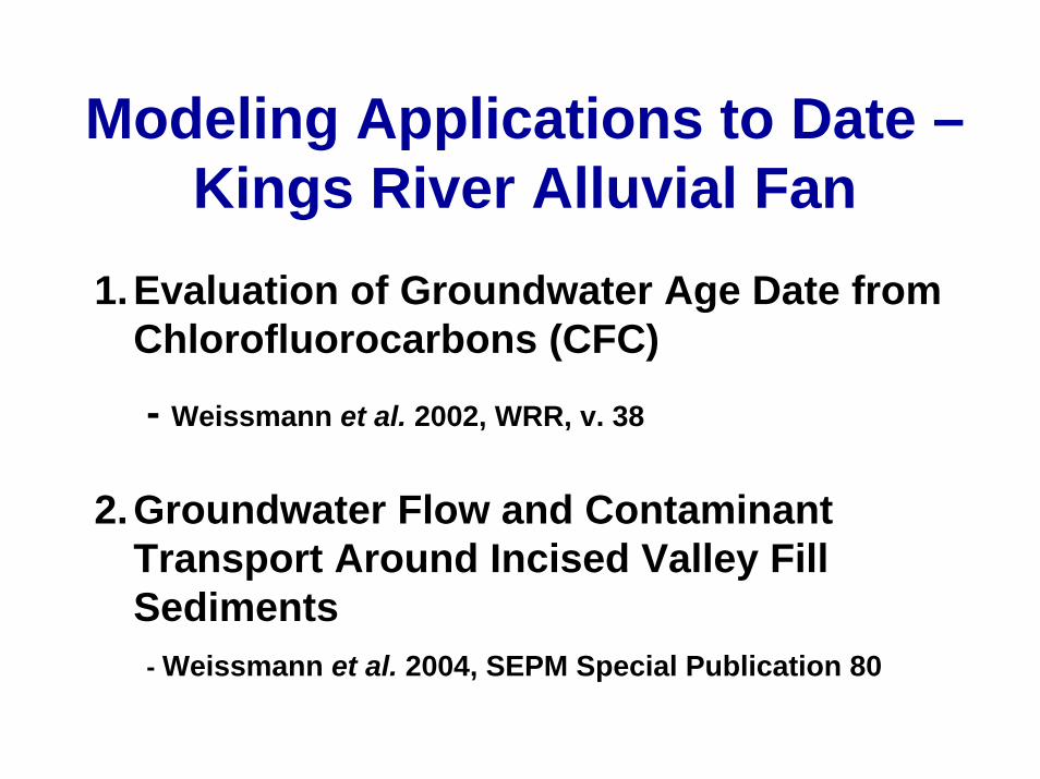
Modeling Applications to Date –Kings River Alluvial Fan
1.Evaluation of Groundwater Age Date from Chlorofluorocarbons (CFC)
- Weissmann et al. 2002, WRR, v. 38
2.Groundwater Flow and Contaminant Transport Around Incised Valley Fill Sediments- Weissmann et al. 2004, SEPM Special Publication 80


Release from Well B4-2
0 2000 4000 6000 8000 10000 12000 14000Dip Direction Distance (meter)
10
60
110
Ele
vatio
n (m
eter
)
Age (years) : 10 30 50 70 90
Vertical Exageration: 50:1


Measured vs. Simulated CFC Concentrations

0 2000 4000 6000 8000 10000120001400010 years after releasing 10,000 particles
0
1000
2000
3000
4000
5000
6000
7000
8000
9000
10000
11000
12000
0 2000 4000 6000 8000 10000120001400030 years after releasing 10,000 particles
0
1000
2000
3000
4000
5000
6000
7000
8000
9000
10000
11000
12000
Particle movement around paleovalley fill
Weissmann et al 2004, SEPM Special Publication 80
CONCLUSIONS• Multi-scale, non-stationary models produced:
• Large-scale: deterministic modeling• Intermediate-scale: stochastic modeling in deterministic
stratigraphic framework• Small-scale: stochastic modeling or appropriate
dispersivities
• The transition probability geostatistics approach:• Produces geologically reasonable realizations of aquifer
heterogeneity.• Allows for incorporation of geological concepts into
model development.
• Improved groundwater modeling and contaminant transport simulation.
• Groundwater age date distributions (CFC age dating).• Models of stratigraphic influence.

Top Related