

![LIFE CYCLE ASSESSMENT OF FRP SEISMIC … · LIFE CYCLE ASSESSMENT OF FRP SEISMIC RETROFITTING . ... 2,200 bridges that are in need of seismic retrofitting ... retrofit technique [2].](https://static.fdocuments.us/doc/165x107/5af03a847f8b9ad0618dca9e/life-cycle-assessment-of-frp-seismic-cycle-assessment-of-frp-seismic-retrofitting.jpg)


![Repair of bridges using Fiber Reinforcement Polymers (FRP) ria.pdf · PDF fileTable 7: Rebar Stresses from Static Tests (MPa) [46] ... Fiber reinforced polymer composites (FRP), developed](https://static.fdocuments.us/doc/165x107/5ab34df47f8b9ac66c8e30d4/repair-of-bridges-using-fiber-reinforcement-polymers-frp-7-rebar-stresses-from.jpg)


Languages
Pages
Legal


Application of FRP materials in Culvert
Road Bridges
A feasibility study with focus on mechanical behavior and life-
cycle cost analysis
Master of Science Thesis in the Master’s Programme Structural Engineering and
Building Technology
JINCHENG YANG
LINA KALABUCHOVA
Department of Civil and Environmental Engineering
Division of Structural Engineering
Steel and Timber Structures
CHALMERS UNIVERSITY OF TECHNOLOGY
Göteborg, Sweden 2014
Master’s Thesis 2014:123


MASTER’S THESIS 2014:123
Application of FRP materials in Culvert Road Bridges
A feasibility study with focus on mechanical behavior and life-cycle cost analysis
Master of Science Thesis in the Master’s Programme Structural Engineering and
Building Technology
JINCHENG YANG
LINA KALABUCHOVA
Department of Civil and Environmental Engineering
Division of Structural Engineering
Steel and Timber Structures
CHALMERS UNIVERSITY OF TECHNOLOGY
Göteborg, Sweden 2014

Application of FRP materials in Culvert Road Bridges
A feasibility study with focus on mechanical behavior and life-cycle cost analysis
Master of Science Thesis in the Master’s Programme Structural Engineering and
Building Technology
JINCHENG YANG
LINA KALABUCHOVA
© JINCHENG YANG & LINA KALABUCHOVA, 2014
Examensarbete / Institutionen för bygg- och miljöteknik,
Chalmers tekniska högskola 2014:123
Department of Civil and Environmental Engineering
Division of Structural Engineering
Steel and Timber Structures
Chalmers University of Technology
SE-412 96 Göteborg
Sweden
Telephone: + 46 (0)31-772 1000
Cover:
Stresses distribution in the FRP culvert structure and FRP culvert bridge, ABAQUS
model
Chalmers Repro Service / Department of Civil and Environmental Engineering
Göteborg, Sweden 2014

I
Application of FRP materials in Culvert Road Bridges
A feasibility study with focus on mechanical behavior and life-cycle cost analysis
Master of Science Thesis in the Master’s Programme Structural Engineering and
Building Technology
JINCHENG YANG
LINA KALABUCHOVA
Department of Civil and Environmental Engineering
Division of Structural Engineering
Steel and Timber Structures
Chalmers University of Technology
ABSTRACT
The aim of the thesis is to investigate the feasibility of using FRP materials in culvert
road bridges. A literature study is carried out to identify the shortcomings of
traditional steel culverts and advantages of FRP materials as a construction material
for manufacture of culverts. A parametric study is carried out on design of a number
of traditional steel culvert bridges and equivalent design is done using FRP sandwich.
Finite element modelling is performed to verify and optimize the preliminary design
of FRP culverts. Furthermore, a life-cycle-cost analysis of two types of culvert that
investigated in this thesis is performed to represent economic advantages of FRP
culverts.
Key words: Culvert, Pettersson-Sundquist design method, FRP, Mechanical behavior,
FE-analysis, Life-cycle cost analysis

II
CHALMERS Civil and Environmental Engineering, Master’s Thesis 2014:123 III
Contents
1 INTRODUCTION 1
Background 1 1.1
Aims and objectives 1 1.2
Methodology and approach 2 1.3
Limitations 2 1.4
2 LITERATURE REVIEW 3
Steel culverts 3 2.1
Steel culverts in Sweden 3 2.1.1
General information of steel culverts 4 2.1.2
Problems of steel culverts 9 2.1.3
Application of FRP materials in civil engineering 11 2.2
Historical perspective of FRP 11 2.2.1
Applications of FRP in structural engineering 12 2.2.2
Applications of FRP in drainage and sewage systems 13 2.2.3
Introduction of FRP materials 15 2.3
Manufacturing processes 16 2.3.1
Matrix constituents 17 2.3.2
Reinforcements 18 2.3.3
Fillers 20 2.3.4
Additives and adhesives 20 2.3.5
Gel coats 21 2.3.6
FRP sandwich panels 21 2.4
Composition of FRP sandwich panels 21 2.4.1
Composition of the study-case FRP sandwich panel 23 2.4.2
Advantages of FRP sandwiches 24 2.4.3
Future outlook of the application of FRP materials 25 2.5
3 DESIGN OF STEEL CULVERTS 27
Introduction 27 3.1
Design cases 27 3.2
Materials 28 3.3
Backfilling soil material 28 3.3.1
Corrugated steel plates 29 3.3.2
Loads 30 3.4
Load effects from the surrounding soil 30 3.4.1
Load effects from live traffic 30 3.4.2
Verification and results 31 3.5
Case 01-08: Pipe-arch culvert 31 3.5.1
Case 09-16: Box culvert 33 3.5.2
CHALMERS, Civil and Environmental Engineering, Master’s Thesis 2014:123 IV
Summary and conclusions 35 3.6
Limitations and assumptions 35 3.7
4 DESIGN OF FRP CULVERTS 36
Introduction 36 4.1
Methodology 36 4.2
Materials of the FRP sandwich panel 38 4.3
FRP laminate face 38 4.3.1
Core material 39 4.3.2
Stiffness and stress analysis of the FRP sandwich 39 4.4
Failure prediction of FRP laminates 40 4.5
Sectional forces in FRP culverts 41 4.6
Hand-calculation based on the SCI method 42 4.6.1
Reliability of hand-calculation 42 4.6.2
Verification by FE-modeling 43 4.6.3
Checks and results 46 4.7
Summary and conclusions 47 4.8
Structural feasibility of FRP culverts 47 4.8.1
Refine the proposed design method for FRP culverts 47 4.8.2
5 LIFE-CYCLE COST ANALYSIS 48
Introduction 48 5.1
LCC analysis of the study-case 49 5.2
Purpose of LCC analysis 49 5.2.1
Assumptions 49 5.2.2
Limitations 49 5.2.3
Agency costs 49 5.3
Initial construction costs 49 5.3.1
Operation and maintenance costs 51 5.3.2
Disposal costs 52 5.3.3
Social costs 52 5.4
User costs 52 5.4.1
Results 53 5.5
Summary 55 5.6
6 CONCLUSIONS 56
About FRP culvert structure 56 6.1
Suggestions for future study 56 6.2
Proposed design method for FRP culvert 56 6.2.1
Applicability of FRP culverts 57 6.2.2
Other materials for FRP culverts 57 6.2.3
Life-cycle assessment in the LCC analysis 57 6.2.4

CHALMERS Civil and Environmental Engineering, Master’s Thesis 2014:123 V
7 REFERENCES 58
8 APPENDICES 61

CHALMERS, Civil and Environmental Engineering, Master’s Thesis 2014:123 VI
Preface
The master thesis was carried out in the Division of Structural Engineering at
Chalmers University of Technology from January 2014 to June 2014.
We would like to give a great thanks to our supervisor and examiner, Assistant
Professor Reza Haghani at Chalmers, for his consistent help during the whole thesis
project. We would also like to thank the supervisor from WSP at Göteborg, Kristoffer
Ekholm, for giving us precious support for the design of steel culverts. Thanks to the
supervisor, Associate Professor Mohammad Al-Emrani, for his critical comments and
constructive suggestions in future. We also express our gratitude to our supervisor
Valbona Mara, the Ph.D. student in the Division of Structural Engineering who shared
her experience and ideas about FRP materials and the life-cycle cost analysis.
Finally, a special thanks to our opponent group Chanthoeun Chiv and Yubath Vocal
Vasquez. We get lots of inspiration from the discussion and idea-sharing about the
design of FRP materials through the entire thesis work.
Göteborg July 2014
Jincheng Yang & Lina Kalabuchova
CHALMERS Civil and Environmental Engineering, Master’s Thesis 2014:123 VII
Notations
Notations in the structural design of culverts
Roman letters
Abolt Cross-sectional area of the bolt
abolt Distance between two parallel rows of bolts (center to center)
As Cross-sectional area of steel profile
As.cor Cross-sectional area of steel profile in the corner region of the culvert
As.top Cross-sectional area of steel profile in the top region of the culvert
Cmy.0, Cmy Calculation parameter for uniform moment factor
Cyy Equivalent uniform moment factor according to EN 1993-1-1
csp Corrugation length of steel profile
Cu Uniformity coefficient
D Span of the culvert
dbolt Diameter of the bolt
d10 Aggregate size at 10% passsing
d50 Aggregate size at 50% passsing
d60 Aggregate size at 60% passsing
e1 Soil void ratio
Es Elastic modulus of steel material
Esoil.d Design value of the tangent modulus of soil material
Esoil.k Characteristic value of the tangent modulus of soil material
esp Calculation parameter of steel profile
Fb.Rd Bearing resistence per bolt
Fst, Ft.Ed Tension in the bolt due to external bending moment
Fsv, Fv.Ed Shear in the bolt due to external normal force
Ft.Rd Tensile force resistance per bolt
fub Ultimate strength of steel material for bolts
Fv.Rd Shear resistence per bolt
fyb Yielding strength of steel material for bolts
f1 Calculation parameter for bending moment
f2.cover Calculation parameter for bending moment
f2.surr Calculation parameter for bending moment
f4', f4'', f4''', f4IV Calculation parameters for bending moment

CHALMERS, Civil and Environmental Engineering, Master’s Thesis 2014:123 VIII
fuk Characteristic value of ultimate strength of steel material
fyd Design value of yielding strength of steel material
fyk Characteristic value of yielding strength of steel material
H Vertical distance between the crown of the culvert and the height at
which the culvert has its greatest width
hf Vertical distance between bolted connection and surface of soil cover
hc height of soil cover
hc.red Reduced height of soil cover
hcorr Profile height
Is Moment of inertia of the cross-section
Is.cor Moment of inertia of the cross-section in the corner region of the
culvert
Is.top Moment of inertia of the cross-section in the top region of the culvert
kv Calculation parameter of soil material
kyy Interaction factor according to EN 1993-1-1
m1 Soil modulus number
Md.SLS.1 Design value of bending moment when the backfilling reaches crown
level in SLS
Md.SLS.2 Design value of bending moment when the backfilling completed in
SLS
Md.ULS.2 Design value of bending moment when the backfilling completed in
ULS
Ms.cover Bending moment due to soil cover
Ms.surr Bending moment due to backfilling soil till crown level
Mt Bending moment due to live traffic
Mt.fatigue Bending moment due to live traffic considering fatigue
mtt Tangential length of steel profile
Mu Plastic moment capacity of the steel profile
Mucr Plastic moment capacity of the steel profile considering buckling
My.Ed Bending moment in the maximum loaded section
My.Ed.cor Bending moment in the corner region
nbolt number of bolts
Nd.u Design value of the maximum normal force in ULS

CHALMERS Civil and Environmental Engineering, Master’s Thesis 2014:123 IX
Nobs Number of heavy vehicles per year per slow lane
npl Calculation parameter for uniform moment factor
NEd Normal force in the maximum loaded section
NEd.cor Normal force in the corner region
Ncover Normal force due to soil cover
Ncr, Ncr.y Critical buckling load
Ncr.el Critical buckling load under idea elastic conditions
Nd.SLS.1 Design value of normal force when the backfilling reaches crown
level in SLS
Nd.SLS.2 Design value of normal force when the backfilling completed in SLS
Nd.ULS.2 Design value of normal force when the backfilling completed in ULS
Nsurr Normal force due to surrounding soil
Nt Normal force due to live traffic load
Nt.fatigue Normal force due to traffic load considering fatigue
Nu Plastic normal force capacity of the steel profile
ptraffic.fatigue Equivalent line load due to fatigue
ptraffic Equivalent line load due to traffic group
Q0, N0 Traffic volume values according to EN 1993-2
Qm1 Average gross weight of lorries in the slow lane
r Radius of curvature of steel profile to section center
Rb
Bottom radius of the culvert
Rc
Corner radius of the culvert
rd Dynamic amplification factor
RP Degree of compaction
Rs Side radius of the culvert
Rsp Radius of curvature of steel profile
Rt Top radius of the culvert
Stiffsoil Calculation parameter of stiffness
Stiffsteel Calculation parameter of stiffness
Sv.1 Calculation parameter considering arching effect of soil
tLd Design life of the culvert bridge
ts Thickness of the corrugated steel plate
wy Ratio of plastic to elastic section modulus according to EN 1993-1-1
CHALMERS, Civil and Environmental Engineering, Master’s Thesis 2014:123 X
Ws Elastic section modulus of the cross-section
Ws.cor Elastic section modulus of the cross-section in the corner region of the
culvert
Ws.top Elastic section modulus of the cross-section in the top region of the
culvert
Zs Plastic section modulus of the cross-section
Zs.cor Plastic section modulus of the cross-section in the corner region of the
culvert
Zs.rein Plastic section modulus of the cross-section with one more
reinforcement plate
Zs.top Plastic section modulus of the cross-section in the top region of the
culvert
Greek letters
α Corrugation Angle of steel profile
αbu Imperfection factor according to EN 1993-1-1
αc Calculation parameter according to BSK 99
β Soil stress exponent
γFf Partial factor for fatigue load
γG.s Partial factor for permanent load in SLS
γG.u Partial factor for permanent load in ULS
γm.soil Partial factor for soil material according to SDM manual
γm.steel Partial factor for steel material according to SDM manual
γM1 Partial factor for steel material according to Eurocode
γMf Partial factor for steel material considering fatigue
γn Safty class factor
γQ.s Partial factor for live load in SLS
γQ.u Partial factor for live load in ULS
δmax Maximum theoretical deflection
ΔFd.t Design value of tensile force in each bolt
ΔFd.v Design value of shear force in each bolt
ΔMt.f Design value of fatigue moment
ΔNt.f Design value of fatigue normal force
Δζbott Effective stress range for bottom fiber

CHALMERS Civil and Environmental Engineering, Master’s Thesis 2014:123 XI
Δζc Detail category for tension
Δζc.p Plate section category
ΔζE.2.b Tensile stress per bolt for fatigue
ΔζE.2.p Damage equivalent stress range related to 2 million cycles
Δζp Effective stress range
Δζtop Effective stress range for top fiber
Δηc Detail category for shear
ΔηE.2.b Shear stress per bolt for fatigue
Η Ratio of plastic to elastic section modulus
Κ Calculation parameter considering arching effect of soil
Κ, ξ, ηj, μ, ω Calculation parameters for buckling in the maximum loaded region
λ Damage equivalence factor for fatigue according to EN 1993-2
λ1 Factor for damage effect of traffic
λ2 Factor for traffic volume
λ3 factor for design life for the bridge
λ4 Factor for traffic in the other lanes
λbuk Relative slenderness according to EN 1993-1-1
λf Relative stiffness between culvert structure and the surrounding soil
ν Poisson ratio of soil material
ρ1 Density of the soil material up to crown height
ρ2 Mean density of the soil material within region (hc+H)
ρcv Mean density of the soil material above crown
ρopt Optimum density of backfilling soil
ζSLS.1 Design value of normal force when the backfilling reaches crown
level in SLS
ζSLS.2 Design value of normal force when the backfilling completed in SLS
ζSLS.max Design value of normal force in the most unfavorable case in SLS
Φ Calculation parameter for flexural buckling
ϕ2 Damage equivalent impact factor
θk Characteristic value of friction angle of the soil material
θk.d Design value of friction angle of the soil material
χy Reduction factor for flexural buckling according to EN 1993-1-1

CHALMERS, Civil and Environmental Engineering, Master’s Thesis 2014:123 XII
Notations in the design of FRP materials
Roman letters
[A] Extensional stiffness matrix for the FRP sandwich
[B] Coupling stiffness matrix for the FRP sandwich
[D] Bending stiffness matrix for the FRP sandwich
[Q] Stiffness matrix for one FRP ply
d Thickness of the core part of the FRP sandwich
E11 Design elastic modulus of FRP material in the longitudinal direction
E22 Design elastic modulus of FRP material in the transversal direction
Ek.11 Characteristic longitudinal elastic modulus of FRP material
Ek.22 Characteristic transverse elastic modulus of FRP material
EA The equivalent membrane elastic constants
EIFRP Bending stiffness of the designed FRP sandwich in the span direction
EI The equivalent bending elastic constants
G12 Design in-plane shear modulus of FRP material
Gk.12 Characteristic in-plan shear modulus of FRP material
M Bending moment applied on the designed cross-section of FRP
sandwich
NF Normal force applied on the designed cross-section of FRP sandwich
no Number of plies used for the FRP laminate face
t Thickness of the FRP plies
tface Thickness of the FRP laminate face
Greek letters
γM Partial factor for FRP material
γM1 Partial factor for FRP material considering derivation of properties
γM2 Partial factor for FRP material considering method of manufacturing
γM3 Partial factor for FRP material considering loading conditions
ΔN Increment value of applied load
εmid Midplane strains
θ Fiber orientation angle of each ply
κmid Midplane curvature
ζd.11.c / ζd.11.t Design strength of FRP material in the longitudinal direction under
compression / tension
CHALMERS Civil and Environmental Engineering, Master’s Thesis 2014:123 XIII
ζd.22.c / ζd.22.t Design strength of FRP material in the transverse direction under
compression / tension
ζk.11.c / ζk.11.t Characteristic strength of FRP material in the longitudinal direction
under compression / tension
ζk.22.c / ζk.22.t Characteristic strength of FRP material in the transversal direction
under compression / tension
ηd.12 Design shear strength of FRP material
ηk.12 Characteristic shear strength of FRP material
υ12 Major Poisson's ratio of FRP material
Notations in the life-cycle cost analysis
Δt Driver delay time due to detouring
L Length of affected roadway the cars are driving
N Number of days of roadwork
n Number of the year considered in LCC
r Hourly vehicle operating cost
r Discount rate
Sa Traffic speed during bridge work activity
Sn Normal traffic speed
w Hourly time value of drivers
Abbreviations
BaTMan Swedish Bridge and Tunnel Management
BRO 2011 Swedish Design regulations for bridges
BSK 99 Swedish Design regulations for steel structures
BV Swedish National Rail Administration (Banverket)
CFRP Carbon Fibre Reinforced Polymer
FE Finite Element
FRP Fiber Reinforced Polymer
GFRP Glass Fiber Reinforced Polymer
KTH The Royal Institute of Technology
LCC Life-Cycle Cost
NPV Net Present Value
SCI Soil Culvert interaction

CHALMERS, Civil and Environmental Engineering, Master’s Thesis 2014:123 XIV
SDM Swedish Design Method
SLS Serviceablility Limit State
TRVK Swedish Transport Administration Requirement (Trafikverkets Krav)
ULS Ultimate Limit State
UV Ultraviolet radiation
Example of indices
b bolt
bott bottom
c compression
cor corner
corr corrugation
d design value
f fatigue
k characteristic value
rein reinforcement
s steel
t tension/traffic
u ultimate
v shear
y yielding

CHALMERS, Civil and Environmental Engineering, Master’s Thesis 2014:123 1
1 Introduction
Background 1.1
Steel culvert bridges are already used for more than one hundred years. The versatility of
culverts assert due to their low initial investment, fast manufacture and installation time,
simplicity in the construction methods, aesthetical look and their geometrical adaptability.
Since the application of culvert structures are greatly miscellaneous they can function as
pedestrian, highway, railway and road bridges as well as for the passage of water and traffic
via conduit.
Despite the number of advantages, the steel culvert structures have some shortcomings
regarding maintenance and repair. Most common problems are corrosion, abrasion of
galvanized steel coating, which lead to degradation and weakening of the structure. Repair
and protection against both local and general scour become a routine for the steel culvert
bridges. Many culvert bridges in Sweden have deteriorated to the point where replacement or
repair is required.
In addition, the fatigue problem coming from the live traffic loads is realized to be one of the
governing issues that limit the use of steel culvert structures. In the condition with shallow
soil cover above the culvert, the fatigue becomes even dominant.
Considering the problems involved with traditional steel culverts, substantial demand of a
better solution comes from the construction field.
In this master thesis fibre reinforced polymer (FRP) materials, as a promising alternative for
the culvert structure, are investigated, due to its significant properties and satisfying
performance regarding deterioration and fatigue.
Aims and objectives 1.2
The brief introduction of background gives a clear goal of the thesis, which aims to
investigate whether the application of FRP materials in culvert bridge structures is a feasible
alternative to the traditional corrugated steel plates.
In order to achieve the goal, the following objectives are determined to capture in terms of
mechanical behaviour and economic performance.
Objectives
Structural feasibility of FRP culvert structures in terms of mechanical behaviour
1. Design the representative cases with steel culverts and find out the governing issues.
2. Design the same cases with FRP and study the performance of FRP culvert against the
issue involved in the steel design.
Cost efficiency of FRP culvert structures in terms of economic performance
3. Perform a life-cycle cost (LCC) analysis of a selected case designed with two
alternatives and compare the costs.
CHALMERS, Civil and Environmental Engineering, Master’s Thesis 2014:123 2
Methodology and approach 1.3
Practical approaches are discussed in order of these three objectives.
Objective 1: Design of the steel culvert structure (see Chapter 3)
Determine a collection of design cases with representative conditions
Design the cases with the Swedish Design Method [1]
Objective 2: Design of the FRP culvert structure (see Chapter 4)
Choose a proper case for further design with FRP
Propose a practical design method for the FRP culvert
Verify the results from proposed design method by FE modelling in ABAQUS
Improve the proposed design method based on the verification
Objective 3: LCC analysis (see Chapter 5)
For the same design case, carry out the LCC analysis of using steel culvert and FRP
culvert, respectively
Compare and analyse the economic performance of these two alternative
Limitations 1.4
Limitations of this thesis generally come from two aspects proposed design method for FRP
culvert structures and assumptions in the LCC analysis.
Due to the complexity of FRP materials and lack of developed design manuals for FRP
structures, the thesis mainly focuses on the design and calculation of the FRP material in the
culvert structure. Thus, the verification part of the FRP culvert design includes: 1) the checks
of capacity of FRP material in the ultimate limit state (ULS) and 2) the deflection in the
serviceability limit state (SLS). More checks need to be taken into account in the future
verification, for instance the creep of FRP material, the capacity of core material and interface
between the face and core (Figure 2.30)
Sustainability such as environmental issues and social aspects of alternatives are not discussed
in the life-cycle study.

CHALMERS, Civil and Environmental Engineering, Master’s Thesis 2014:123 3
2 Literature Review
Steel culverts 2.1
Steel culverts in Sweden 2.1.1
The concept of corrugated profile steel pipes was presented in the mid 1950’s. The design was
based on primitive diagrams and standard drawings, which operated with two types of
conduits only: low-rise culverts and vertical ellipses. By then, the standard drawings were
only applicable for the structures with a span up to 5 m. However, several culverts with a span
over 5 meters were also erected.
With an increasing industry, technologies and therefore knowledge about culverts, the more
advanced and accurate design methods were developed, that are able to consider different soil
materials, larger spans and various cover heights. The first full-scale test of pipe arch was
performed by The Royal Institute of Technology (KTH) in 1983 supported by Swedish Road
Administration (Figure 2.1). The structure had as span of 6,1 meters with a cover height of 1
meter. In addition, the other field test of the culvert with span of 6 meters and 0,75-1,5 meters
cover height was carried in 1987-1990 (Figure 2.2).
The tests were followed by a newly proposed Swedish Design Method (SDM) in 2000.
Thereafter, The Swedish Road Administration (Vägverket) implemented the method in the
code Bro 2002 and National Rail Administration (Banverket) accepted it in BV Bro. After
introducing the box culvert to Swedish marked in 2002, actualizing the full-scale field tests,
improving the design methodologies and introducing certain modifications the 4th
edition of
the handbook by Pettersson and Sundquist [1] was published in 2010.
There existed about 4430 culvert bridges in 2012, 4100 whereof are made of steel according
to Swedish Bridge and Tunnel Management (BaTMan). The vast majority of culverts were
built in 50’s and 60’s, which implies that they are in the poor condition and require
rehabilitation or replacement. Moreover, according to the report Safi, 2012 [2] the common
span length for culverts in Sweden are 5 meters and less.
According to TRVK Bro 11 (2011) culverts are commonly designed for the technical life of
80 years; however culverts are constantly exposed to adverse environment, thus making the
inspection and maintenance frequent and service life shorter.
Figure 2.1 The first full-scale test in Sweden in 1983 [3]
CHALMERS, Civil and Environmental Engineering, Master’s Thesis 2014:123 4
Figure 2.2 The field test of pipe arch culvert in Sweden in 1987-1990 [3]
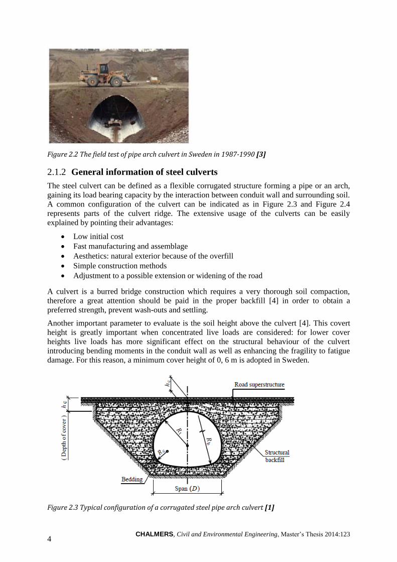
General information of steel culverts 2.1.2
The steel culvert can be defined as a flexible corrugated structure forming a pipe or an arch,
gaining its load bearing capacity by the interaction between conduit wall and surrounding soil.
A common configuration of the culvert can be indicated as in Figure 2.3 and Figure 2.4
represents parts of the culvert ridge. The extensive usage of the culverts can be easily
explained by pointing their advantages:
Low initial cost
Fast manufacturing and assemblage
Aesthetics: natural exterior because of the overfill
Simple construction methods
Adjustment to a possible extension or widening of the road
A culvert is a burred bridge construction which requires a very thorough soil compaction,
therefore a great attention should be paid in the proper backfill [4] in order to obtain a
preferred strength, prevent wash-outs and settling.
Another important parameter to evaluate is the soil height above the culvert [4]. This covert
height is greatly important when concentrated live loads are considered: for lower cover
heights live loads has more significant effect on the structural behaviour of the culvert
introducing bending moments in the conduit wall as well as enhancing the fragility to fatigue
damage. For this reason, a minimum cover height of 0, 6 m is adopted in Sweden.
Figure 2.3 Typical configuration of a corrugated steel pipe arch culvert [1]

CHALMERS, Civil and Environmental Engineering, Master’s Thesis 2014:123 5
Figure 2.4 Different parts of the culvert ridge [5]
2.1.2.1 Culvert profiles
The design of culvert shape considers: 1) the site conditions, such as span and cover height, 2)
flow capacity and fish passage for the river-passage-culvert bridges. The proposal should also
be cost-effective and durable. According to 4th
edition of the handbook by Pettersson and
Sundquist [1], sever types of culvert profile are classified as:
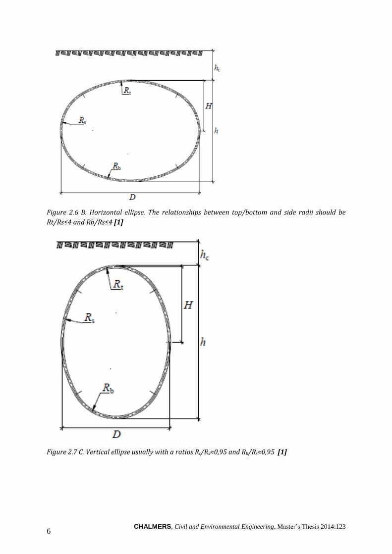
Closed profiles (Figure 2.5 - Figure 2.8):
A. Circular with constant radius
B. Horizontal ellipse
C. Vertical ellipse
D. Pipe-arch, defined by three radii
Arch-type profiles (Figure 2.9 - Figure 2.11):
E. Circular with single radius
F. Two or three radii
G. Box culvert
Figure 2.5 A. Circular profile with constant radius R [1]
CHALMERS, Civil and Environmental Engineering, Master’s Thesis 2014:123 6
Figure 2.6 B. Horizontal ellipse. The relationships between top/bottom and side radii should be
Rt/Rs≤4 and Rb/Rs≤4 [1]
Figure 2.7 C. Vertical ellipse usually with a ratios Rt/Rs≈0,95 and Rb/Rs≈0,95 [1]
CHALMERS, Civil and Environmental Engineering, Master’s Thesis 2014:123 7
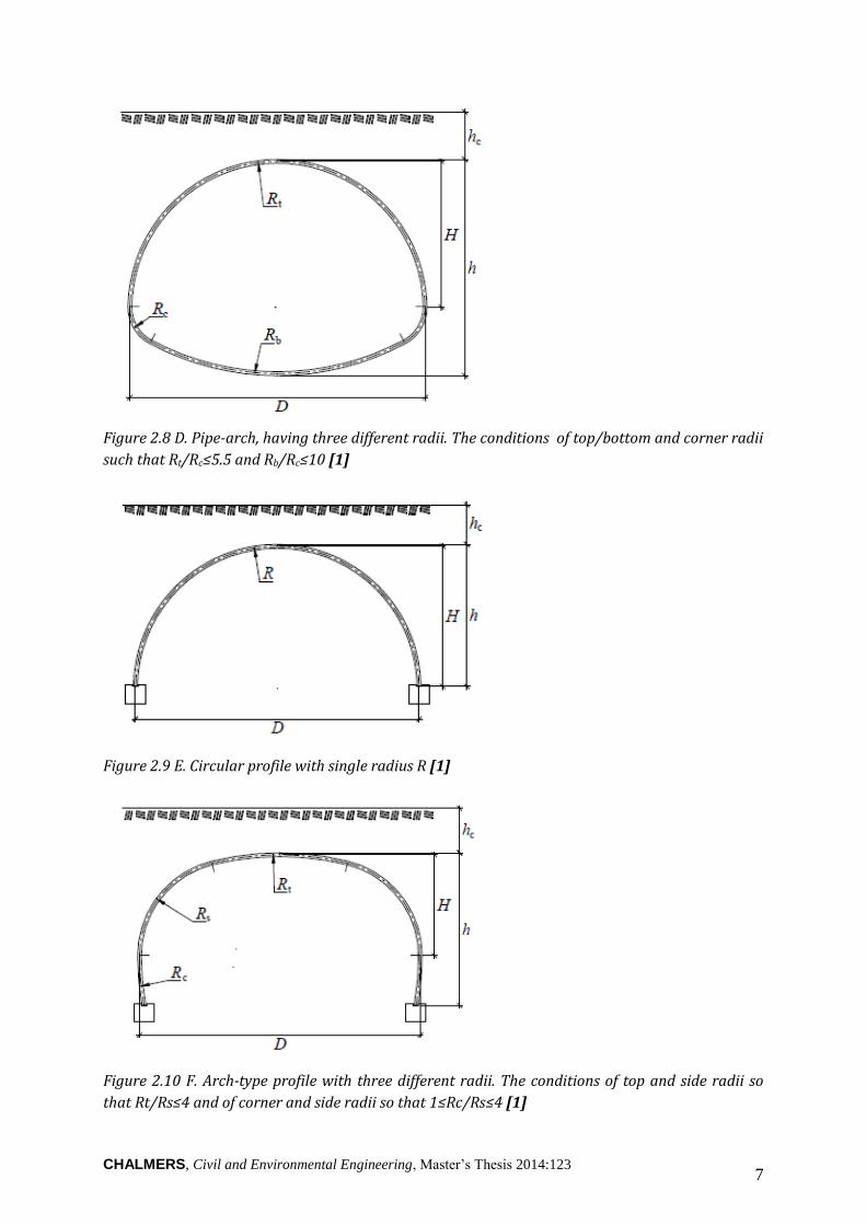
Figure 2.8 D. Pipe-arch, having three different radii. The conditions of top/bottom and corner radii
such that Rt/Rc≤5.5 and Rb/Rc≤10 [1]
Figure 2.9 E. Circular profile with single radius R [1]
Figure 2.10 F. Arch-type profile with three different radii. The conditions of top and side radii so
that Rt/Rs≤4 and of corner and side radii so that 1≤Rc/Rs≤4 [1]

CHALMERS, Civil and Environmental Engineering, Master’s Thesis 2014:123 8
Figure 2.11 G. Box culvert with a relationship Rt/Rs≤12 [1]
The box culverts for strengthening purposes due to critical sections might be reinforced with
plates (Figure 2.12).
Figure 2.12 Box culvert with reinforcing plates [1]
2.1.2.2 Corrugation profiles
Manufacturers offer a wide range of corrugation profiles, but according to the 4th
edition of
the handbook by Pettersson and Sundquist [1], the most typically used are illustrated in Figure
2.13 and the thicknesses vary between 1,5-7 millimetres.
Figure 2.13 Common steel corrugation profiles [1]

CHALMERS, Civil and Environmental Engineering, Master’s Thesis 2014:123 9
Problems of steel culverts 2.1.3
Nowadays, a critical problem of the existing culvert is a threat of sink holes, flooding or road
collapse. The development of a more durable material is much-needed, since replacement or
repair of steel culverts is costly, time-consuming and traffic interruptive. As mentioned
previously, culverts can be used in a variety of conditions, for instance for a road bridge and
stream crossing, aquatic fauna passage and drainage (Figure 2.14), thus the most concerning
issue is corrosion having a significant effect on service life of the structure. The most exposed
location and prone to deteriorate is the invert (Figure 2.15, Figure 2.16), in addition to this,
the damage of protective layer due to road salts might appear especially for aged structures,
allowing the corrosion and annihilation of base metal. Moreover, increased traffic, low quality
of structural members and insufficient maintenance makes the culverts structurally deficient
and/or functionally obsolete. In addition, under certain circumstances, repair might be even
more expensive than replacing with a new one.
Figure 2.14 Culverts for stream crossing and drainage [6]
Figure 2.15 Deteriorated invert and perched end of pipe culvert [7]
CHALMERS, Civil and Environmental Engineering, Master’s Thesis 2014:123 10
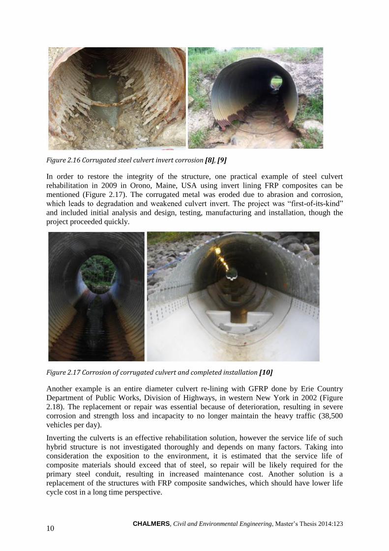
Figure 2.16 Corrugated steel culvert invert corrosion [8], [9]
In order to restore the integrity of the structure, one practical example of steel culvert
rehabilitation in 2009 in Orono, Maine, USA using invert lining FRP composites can be
mentioned (Figure 2.17). The corrugated metal was eroded due to abrasion and corrosion,
which leads to degradation and weakened culvert invert. The project was ―first-of-its-kind‖
and included initial analysis and design, testing, manufacturing and installation, though the
project proceeded quickly.
Figure 2.17 Corrosion of corrugated culvert and completed installation [10]
Another example is an entire diameter culvert re-lining with GFRP done by Erie Country
Department of Public Works, Division of Highways, in western New York in 2002 (Figure
2.18). The replacement or repair was essential because of deterioration, resulting in severe
corrosion and strength loss and incapacity to no longer maintain the heavy traffic (38,500
vehicles per day).
Inverting the culverts is an effective rehabilitation solution, however the service life of such
hybrid structure is not investigated thoroughly and depends on many factors. Taking into
consideration the exposition to the environment, it is estimated that the service life of
composite materials should exceed that of steel, so repair will be likely required for the
primary steel conduit, resulting in increased maintenance cost. Another solution is a
replacement of the structures with FRP composite sandwiches, which should have lower life
cycle cost in a long time perspective.

CHALMERS, Civil and Environmental Engineering, Master’s Thesis 2014:123 11
Figure 2.18 An entire culvert re-lining in Buffalo, New York, USA [11]
Even though culverts made of steel has a number of positive aspects, both regarding
production, construction and structural performance, the most pronounced problem is the
material deterioration due to aggressive environment and construction degradation due to
fatigue. Despite the protective layer that steel is covered, the service life sometimes cannot by
fully utilized, this entails expensive and frequent inspection and repair.
Additionally, due to loading-unloading cycles on the bridge, fatigue is one of the dominant
factors that influence the performance of steel culverts. Therefore, in order to avoid these
time- and money-consuming issues a new alternative of FRP culverts is further studied in this
thesis.
Application of FRP materials in civil engineering 2.2
Historical perspective of FRP 2.2.1
Although the history of FRP composites can be observed back thousands of years ago to
Mesopotamia (present – Iraq), bringing under the use of straw as a reinforcement in mud
brick, it is referred to a more recent times, when the usage of short glass fibre reinforcement
in cement in the United States in the early 1930’s started and the development of FRP, the
composition that we know today, were not developed until the early 1940’s.
As the name of the material itself suggests, FRP is composed from at least two materials:
high-strength fibres embedded in a polymer matrix, thus giving a great-performance
composite material. After World War II, when the FRP was used mainly for defence
industries, the polymer-based composites spread broadly when the fibre reinforcements and
resins became commercially available and affordable. Primarily, FRP automotive industry
introduced composites into vehicle frames in early 1950s. The greatest advantages of the
material are high strength characteristics, corrosion resistance, easy-shaping and lightness,
therefore research emphasized on developing new and improving manufacturing techniques,
such as filament winding and pultrusion, which helped to introduce the usage of composites
into new applications. Other industries such as aerospace started producing pressure vessels,
containers and non-structural aircraft components, marine market applied the material in mine
sweeping vessels, submarine parts and brew boats and recreation industry adopted composites
very well for tennis, golf, fishing and skiing equipment.
The main growth in the application and development of the FRP composites in civil
engineering started in the 1960’s. Two major structures made of glass fibre-reinforced
polymer were built: the dome structure in Benghazi in 1968 and the roof structure in Dubai in
1972, and the other structures followed deliberately. By late 1980’s the military market begin
to vanish and in the early 1990’s the need for old infrastructure to be repaired or replaced
CHALMERS, Civil and Environmental Engineering, Master’s Thesis 2014:123 12
increased as FRP cost decreased simultaneously. Currently the interest in the appliance of the
material is growing, including the research of full-scale experiments, because the long –term
behaviour is still not explored conclusively, also focusing on the optimisation of structures
using finite element analysis approaches.
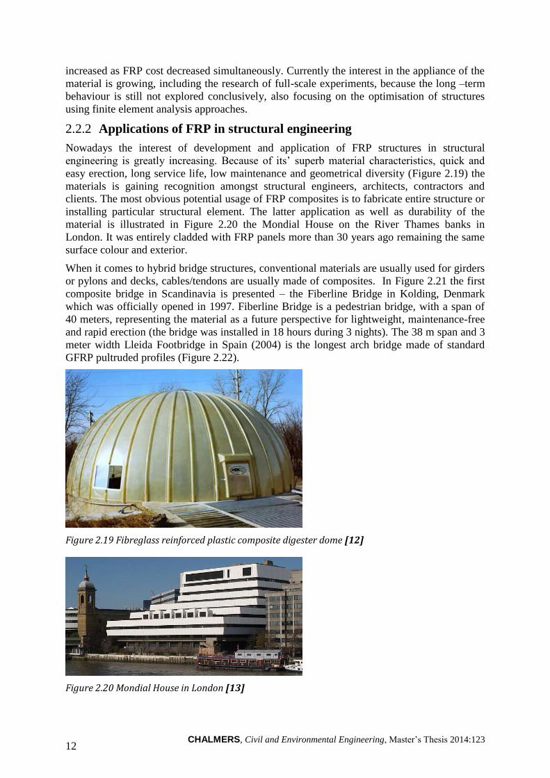
Applications of FRP in structural engineering 2.2.2
Nowadays the interest of development and application of FRP structures in structural
engineering is greatly increasing. Because of its’ superb material characteristics, quick and
easy erection, long service life, low maintenance and geometrical diversity (Figure 2.19) the
materials is gaining recognition amongst structural engineers, architects, contractors and
clients. The most obvious potential usage of FRP composites is to fabricate entire structure or
installing particular structural element. The latter application as well as durability of the
material is illustrated in Figure 2.20 the Mondial House on the River Thames banks in
London. It was entirely cladded with FRP panels more than 30 years ago remaining the same
surface colour and exterior.
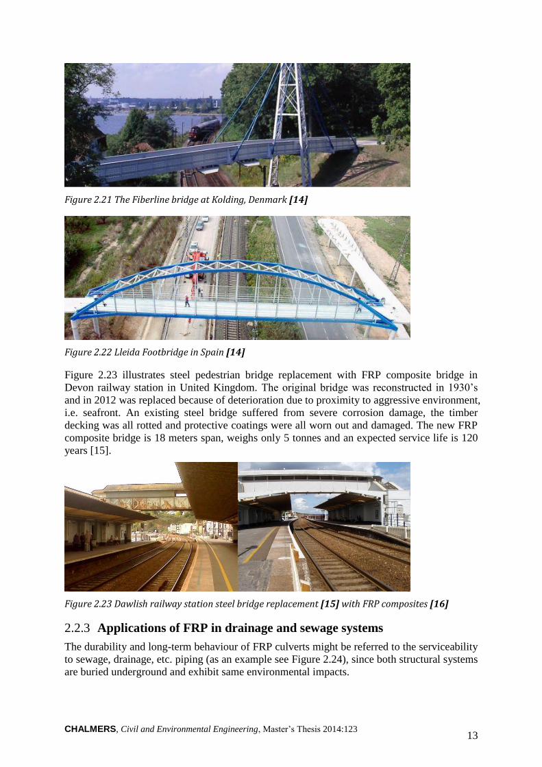
When it comes to hybrid bridge structures, conventional materials are usually used for girders
or pylons and decks, cables/tendons are usually made of composites. In Figure 2.21 the first
composite bridge in Scandinavia is presented – the Fiberline Bridge in Kolding, Denmark
which was officially opened in 1997. Fiberline Bridge is a pedestrian bridge, with a span of
40 meters, representing the material as a future perspective for lightweight, maintenance-free
and rapid erection (the bridge was installed in 18 hours during 3 nights). The 38 m span and 3
meter width Lleida Footbridge in Spain (2004) is the longest arch bridge made of standard
GFRP pultruded profiles (Figure 2.22).
Figure 2.19 Fibreglass reinforced plastic composite digester dome [12]
Figure 2.20 Mondial House in London [13]
CHALMERS, Civil and Environmental Engineering, Master’s Thesis 2014:123 13
Figure 2.21 The Fiberline bridge at Kolding, Denmark [14]
Figure 2.22 Lleida Footbridge in Spain [14]
Figure 2.23 illustrates steel pedestrian bridge replacement with FRP composite bridge in
Devon railway station in United Kingdom. The original bridge was reconstructed in 1930’s
and in 2012 was replaced because of deterioration due to proximity to aggressive environment,
i.e. seafront. An existing steel bridge suffered from severe corrosion damage, the timber
decking was all rotted and protective coatings were all worn out and damaged. The new FRP
composite bridge is 18 meters span, weighs only 5 tonnes and an expected service life is 120
years [15].
Figure 2.23 Dawlish railway station steel bridge replacement [15] with FRP composites [16]
Applications of FRP in drainage and sewage systems 2.2.3
The durability and long-term behaviour of FRP culverts might be referred to the serviceability
to sewage, drainage, etc. piping (as an example see Figure 2.24), since both structural systems
are buried underground and exhibit same environmental impacts.
CHALMERS, Civil and Environmental Engineering, Master’s Thesis 2014:123 14
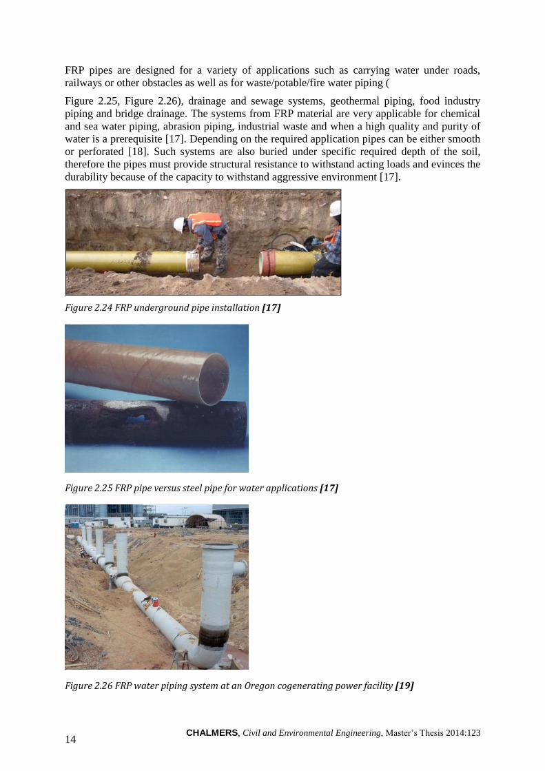
FRP pipes are designed for a variety of applications such as carrying water under roads,
railways or other obstacles as well as for waste/potable/fire water piping (
Figure 2.25, Figure 2.26), drainage and sewage systems, geothermal piping, food industry
piping and bridge drainage. The systems from FRP material are very applicable for chemical
and sea water piping, abrasion piping, industrial waste and when a high quality and purity of
water is a prerequisite [17]. Depending on the required application pipes can be either smooth
or perforated [18]. Such systems are also buried under specific required depth of the soil,
therefore the pipes must provide structural resistance to withstand acting loads and evinces the
durability because of the capacity to withstand aggressive environment [17].
Figure 2.24 FRP underground pipe installation [17]
Figure 2.25 FRP pipe versus steel pipe for water applications [17]
Figure 2.26 FRP water piping system at an Oregon cogenerating power facility [19]

CHALMERS, Civil and Environmental Engineering, Master’s Thesis 2014:123 15
There are considerable number of advantages for usage FRP pipes [20]:
Fatigue endurance
Corrosion resistant in comparison with ordinary steel
High mechanical and impact strength
Temperature resistant
Smooth internal pipe surface (low friction coefficient)
Abrasion resistant
Lightweight, therefore easy handling, lower transportation costs and fast installation
Low service life cost, due to reduced installation and maintenance investments
Increased serviceability
Shape complexity
The general inspection of FRP pipes are similar to steel piping when checking positional
deviation, mechanical damage (mainly in the area of invert, resulting in reduced wall
thickness), erosion wear, deformation, flow obstacles, connections. However the maintenance
of FRP piping includes specific controls (containing particular tools and methods) [21]:
Flange and bottom flatness
Laminate and ply thickness
Aging damage: delamination, cracking, etc.
Heat-related damage
The durability of FRP piping are already well known and proven [17], therefore with the
reference to advantages stated above, a stable foundation can be placed for further research in
application of FRP material, which in this thesis study-case is the culvert structure.
Introduction of FRP materials 2.3
Fibre Reinforced Polymer (FRP) composites can be defined as combination of at least two
individual materials (Figure 2.27): a matrix, either thermoset or thermoplastic, and a fibrous
or other reinforcing material with a certain aspect ratio (length to thickness) to provide a
considerable reinforcement in one or more directions. Each of these different agents has its
own function to perform, i.e. the fibres provide strength and stiffness and matrix contributes
in a rigidity and environmental protection, hence the composite system performs sufficiently
as one unit (Figure 2.28). FRP may also contain fillers which reduce cost and shrinkage as
well additives that improve mechanical and physical properties and workability of the final
composite [22].
Moreover, FRP composites are anisotropic, meaning that the best mechanical properties are in
the direction of the fibre arrangement, whilst other construction materials, e.g. steel is
isotropic.

CHALMERS, Civil and Environmental Engineering, Master’s Thesis 2014:123 16
Figure 2.27 Basic components to create FRP composite [23]
Figure 2.28 The combination of matrix and fibres gives a composite material with superior
properties [23]
Advantages
The selection and usage of FRP composites includes such advantages [24], [25]:
- High strength
- Lightweight (75% less than steel)
- Electromagnetically neutral
- UV resistant
- Withstands freeze-thaw cycles
- Anisotropic; the ability to obtain required mechanical properties
- Low maintenance
- Durable: high corrosion and fatigue resistance
- Geometrical diversity
- Dimensional stability
- Simple and rapid installation, therefore cost effective
- Compatible with conventional construction materials
Manufacturing processes 2.3.1
The manufacturing process, as well as the composites constituents, plays a very important part
in assessing the characteristics of the final product. In addition, such manufacturing process
should be chosen so that optimal properties of the composite and economical alternative are
attained. Purchaser demands, structural and architectural requirements, production rate and
assembly/erection possibilities should be considered as well. According to ―The International
Handbook of FRP Composites in Civil Engineering‖ by Zoghi [22], manufacturing processes
can be classified into three categories:
Manual processes, i.e. wet lay-up and contact moulding

CHALMERS, Civil and Environmental Engineering, Master’s Thesis 2014:123 17
Semi- automated processes, i.e. compression moulding and resin infusion.
Automated processes, i.e. pultrusion, filament winding, injection moulding
Matrix constituents 2.3.2
As a matrix for the composites, resins are used and functions as a binder for the reinforcement,
transfers stresses between the reinforcing fibres and protects the fibres from mechanical or
environmental damage. Resins are classified into thermoplastics and thermosets [22].
Thermoplastic resins remain solid at room temperature, become fluid when temperature
increase and solidifies when cooled. There is no chemical reaction; the material change is
totally physical. Thermoset resins undergo an irreversible chemical reaction; after curing they
cannot be converted back to the original liquid form, therefore being a desirable agent for
structural applications. Resins should be chosen taking into account the application field, the
extent that structure is exposed to environment and temperature, manufacturing method,
curing conditions and required properties. The most common thermosetting resins used in the
composite market [25]:
Unsaturated polyester
Epoxy
Vinyl ester
Phenolic
Polyurethane
Unsaturated polyester
The vast majority of composites applied in industry are unsaturated polyesters which is
approximately 75 % of the total resins used. During the building of the polymer chains,
polyesters can be formulated and chemically tailored to provide desired properties and
process compatibility, hereby making the material greatly versatile. The advantages of the
unsaturated polyester are its affordable price, dimensional stability, easy to handle during
manufacturing process, corrosion resistant and can serve as a fire retardant.
Epoxy
Epoxy resins are well-known for their extensive application of composite parts, structures and
concrete repair. The utmost merit of the resins over unsaturated polyesters are their
workability, low-shrinkage, environmental durability and have a higher shear strength than
polyesters. Binding the agent with different materials or incorporating with other epoxy resins
specific performance characteristics can be achieved. Epoxies are used in the production of
high performance composites with improved mechanical, electrical and thermal properties,
better environment and corrosion resistance. Nevertheless, epoxies have poor UV resistance
and due to higher viscosity post-curing (elevated heat) is required to attain the ultimate
mechanical properties. Epoxies are operated along with fibrous reinforcing materials, e. g.
glass and carbon.
Vinyl ester
Vinyl esters were developed taking the advantages of workability of the epoxies and fast
curing of the polyesters. An outcome of such material is that it is cheaper than epoxies but has
a higher physical performance than polyesters. Moreover, this composite is mechanically stiff,
very workable and offers superb corrosion, heat and moisture resistance and fast curing.
Phenolic
CHALMERS, Civil and Environmental Engineering, Master’s Thesis 2014:123 18
Phenolic resins performs well in elevated temperatures, low emission of toxic fumes, they are
creep and corrosion resistant, excellent thermal and effective sound insulation. The resins
have lower shrinkage in comparison with polyesters.
Polyurethane
Polyurethanes arise in an astonishing diversity of forms; they are used as adhesives, foams,
coatings or elastomers. Advantages of polyurethane adhesives are impact and environmental
resistant, rapid curing and well binding with various surfaces. Polyurethane foams optimize
the density for insulation, architectural and structural components, such as sandwich panels.
Polyurethanes used for coatings are stiff, but flexible, chemical-proof and fast curing.
Elastomers can be characterized as especially tough and abrasive in wheels, bumper
components or insulation.
Reinforcements 2.3.3
Fibres are used to convey structural strength and thickness to a composite material. The fibres
commonly occupies 30 – 70 % of the matrix volume in the composite, thence a considerable
amount of effort was put in the research and development of the performance in the types,
orientation, volume fraction and composition. Obviously, the most desirable characteristics
for the composites are strength, stiffness and toughness, which are highly dependent on the
type and geometry of the reinforcement.
Reinforcements can be either type of natural and man-made, however most commercial are
man-made; correlating to the price respectively, glass, carbon and aramid fibres are usually
used for composites in the structural applications [25].
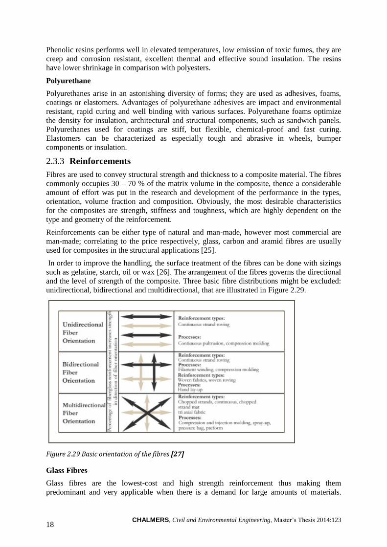
In order to improve the handling, the surface treatment of the fibres can be done with sizings
such as gelatine, starch, oil or wax [26]. The arrangement of the fibres governs the directional
and the level of strength of the composite. Three basic fibre distributions might be excluded:
unidirectional, bidirectional and multidirectional, that are illustrated in Figure 2.29.
Figure 2.29 Basic orientation of the fibres [27]
Glass Fibres
Glass fibres are the lowest-cost and high strength reinforcement thus making them
predominant and very applicable when there is a demand for large amounts of materials.

CHALMERS, Civil and Environmental Engineering, Master’s Thesis 2014:123 19
Along with these advantages glass fibres are also corrosion resistant, tough and chemical inert.
However, the fibres possess some disadvantages:
Low modulus of elasticity
Poor abrasion resistance, therefore manufactured with various surface covers
Poor adhesion to resins, requiring chemical coupling agents, e.g. silane
Even though the material creeps under sustained loading, the design can be made so that the
composite performance would be satisfactory. In the application where stiffness is crucial, the
design of the glass fibres must be specially treated.
There are various types of glass fibres for different kinds of application:
―A‖ or ―AR‖ stands for alkane resistance
―C‖ may be selected when better chemical resistance is required, but they have a
slightly lower strength compared to ―E‖ type
―E‖ used to improve electrical properties; most extensively used for its high tensile
strength and durability
―S‖ or ―R‖ stands for higher strength, stiffness and elevated temperature resistant, but
more expensive than ―E‖ fibres
Glass fibres are regarded as an isotropic material, having equal or better characteristics than
steel in particular forms. The material weights more than carbon or aramid, but generally has
a fine impact resistance.
Carbon Fibre
Despite high specific strength and stiffness, the applications in construction of carbon fibres
are quite limited because of their high cost. However, the first two properties makes it an ideal
material where the lightweight is important, e.g. aircraft applications. Carbon fibres are also
very convenient to use in a critical applications such as concrete beam/column or seismic
rehabilitation and retrofitting. The fibres are assumed as anisotropic; stronger and stiffer in
longitudinal direction than in transverse, in addition to high fatigue and creep resistance as
well as favourable coefficient of thermal expansion.
Similarly to glass fibres, carbon fibres’ surface is also chemically treated with coatings and
chemical coupling agents before any further processing. Carbon composites shows higher
performance when adhesively bonded rather than mechanically fastened, because of
phenomenon when the composite exhibits stress concentrations that are caused by material
brittleness due to higher modulus. Moreover, when used together with metals carbon fibres
can cause corrosion, therefore a barrier materials such as glass or resin are used to overcome
this.
Aramid Fibre
Aramid fibres are the best known organic fibres and are often used for ballistic and impact
applications. Aramid characteristics:
Good mechanical properties at low density
Tough and damage resistant
Quite high tensile strength
Medium modulus of elasticity
Very low density in comparison with glass and carbon
Electrical and heat insulator
Resistant to organic solvents, fuels, lubricants
Ductile

CHALMERS, Civil and Environmental Engineering, Master’s Thesis 2014:123 20
Good fatigue and creep resistance
In comparison with glass, aramids offers higher tensile strength and approximately 50%
higher modulus, however has a low-performance regarding compressive strength in
comparison with two latter fibres, it is also costly, susceptible to UV light and temperature
changes.
Fillers 2.3.4
Fillers are used to fill up the voids in a matrix, because of the high price of resins, therefore
enhancing mechanical, physical and chemical performance of the composite. The main types
of fillers [26] used in the market:
Calcium carbonate is a low-cost material available in a variety of particle size,
therefore the most widely used inorganic filler.
Kaolin can also be offered in a wide range of particle size, thus the second mostly used
filler.
Alumina trihydrate is commonly used to enhance the performance of the composite
during fire and smoke. The principle is that that when this filler is exposed to high
temperatures it gives off water (hydration), hereby reducing the spread of the flame
and smoke.
Calcium sulphate is the major flame/smoke decelerator, releasing water at lower
temperatures.
If the fillers are used properly, improved characteristics may include:
Better performance during fire or chemical action
Higher mechanical strength
Lower shrinkage
Stiffness
Fatigue and creep resistance
Lower thermal expansion and exothermic coefficients
Water, weather and temperature resistance
Surface smoothness
Dimensional stability
However, when the high strength composites are formulated, they should not contain fillers,
because of the difficulty to fully wet out the heavy fibre reinforcement, due to increased
viscosity of the resin paste.
Additives and adhesives 2.3.5
Additives modify material properties, improve the performance of composite and
manufacturing process and are used in low quantities in comparison with other constituents.
When put to the composites, additives usually increase the cost of the material system as well
as the usefulness and durability of the product. The type of additives available:
Catalysts, promoters, inhibitors – accelerated the speed of the curing
Colorants – provide colour
Release agents – facilitate the removal of the moulds
Thixotropic agents – reduces the flow or drain of the resin from the surfaces
CHALMERS, Civil and Environmental Engineering, Master’s Thesis 2014:123 21
Adhesives are used to bind composites to themselves as well to the other surfaces. In order to
get a proper connection, surface must be carefully treated to ensure the bond strength. The
most common adhesives are epoxy, acryl and urethane [26].
Gel coats 2.3.6
Gel coats provide an environmental and impact resistant surface finishing [25]. The thickness
is determined depending on the intended application of the composite product. Gel coats
provide no additional structural capacity, therefore they should be resilient; sustain
deformations from the structure and do not crack due to temperature changes, be impenetrable
and UV light proof, provide a colour scheme. They should enhance chemical, abrasion, fire
and moisture resistance.
FRP sandwich panels 2.4
Composition of FRP sandwich panels 2.4.1
The composition of FRP laminates and core materials is defined as a sandwich structure. FRP
sandwich panels with requisite mechanical properties can be designed depending on the
intended use. The manufacturing process, type, distribution/orientation, bonding, of the
materials, geometry, quantity/volume, orientation of the reinforcement and cost of products
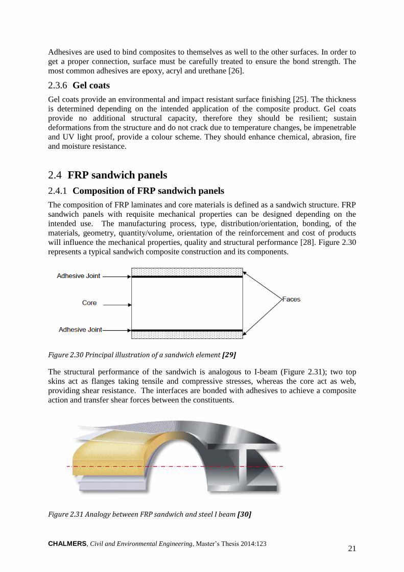
will influence the mechanical properties, quality and structural performance [28]. Figure 2.30
represents a typical sandwich composite construction and its components.
Figure 2.30 Principal illustration of a sandwich element [29]
The structural performance of the sandwich is analogous to I-beam (Figure 2.31); two top
skins act as flanges taking tensile and compressive stresses, whereas the core act as web,
providing shear resistance. The interfaces are bonded with adhesives to achieve a composite
action and transfer shear forces between the constituents.
Figure 2.31 Analogy between FRP sandwich and steel I beam [30]
CHALMERS, Civil and Environmental Engineering, Master’s Thesis 2014:123 22
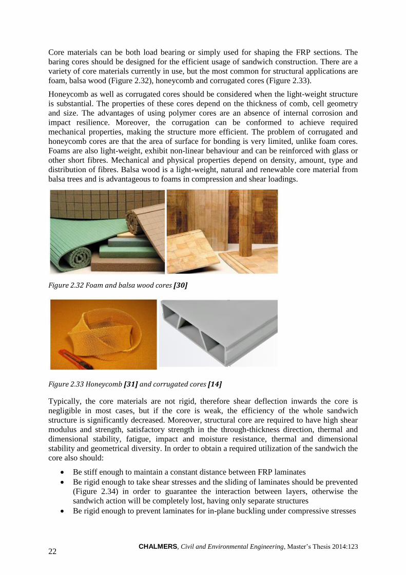
Core materials can be both load bearing or simply used for shaping the FRP sections. The
baring cores should be designed for the efficient usage of sandwich construction. There are a
variety of core materials currently in use, but the most common for structural applications are
foam, balsa wood (Figure 2.32), honeycomb and corrugated cores (Figure 2.33).
Honeycomb as well as corrugated cores should be considered when the light-weight structure
is substantial. The properties of these cores depend on the thickness of comb, cell geometry
and size. The advantages of using polymer cores are an absence of internal corrosion and
impact resilience. Moreover, the corrugation can be conformed to achieve required
mechanical properties, making the structure more efficient. The problem of corrugated and
honeycomb cores are that the area of surface for bonding is very limited, unlike foam cores.
Foams are also light-weight, exhibit non-linear behaviour and can be reinforced with glass or
other short fibres. Mechanical and physical properties depend on density, amount, type and
distribution of fibres. Balsa wood is a light-weight, natural and renewable core material from
balsa trees and is advantageous to foams in compression and shear loadings.
Figure 2.32 Foam and balsa wood cores [30]
Figure 2.33 Honeycomb [31] and corrugated cores [14]
Typically, the core materials are not rigid, therefore shear deflection inwards the core is
negligible in most cases, but if the core is weak, the efficiency of the whole sandwich
structure is significantly decreased. Moreover, structural core are required to have high shear
modulus and strength, satisfactory strength in the through-thickness direction, thermal and
dimensional stability, fatigue, impact and moisture resistance, thermal and dimensional
stability and geometrical diversity. In order to obtain a required utilization of the sandwich the
core also should:
Be stiff enough to maintain a constant distance between FRP laminates
Be rigid enough to take shear stresses and the sliding of laminates should be prevented
(Figure 2.34) in order to guarantee the interaction between layers, otherwise the
sandwich action will be completely lost, having only separate structures
Be rigid enough to prevent laminates for in-plane buckling under compressive stresses
CHALMERS, Civil and Environmental Engineering, Master’s Thesis 2014:123 23
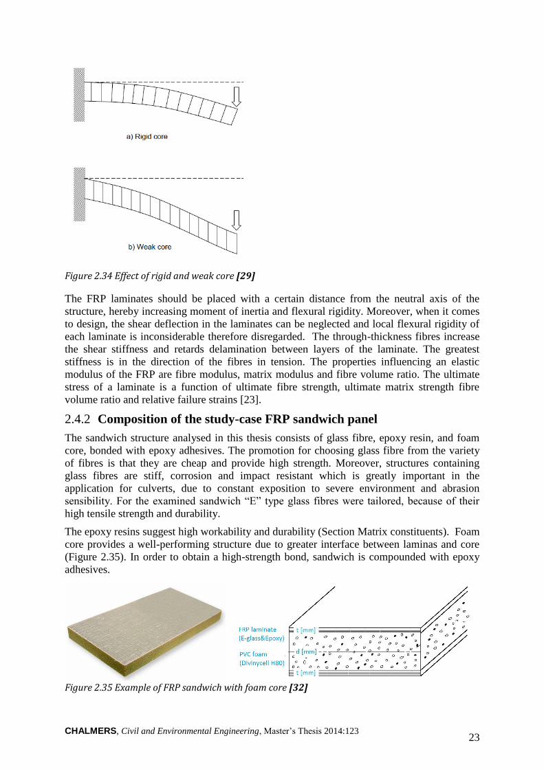
Figure 2.34 Effect of rigid and weak core [29]
The FRP laminates should be placed with a certain distance from the neutral axis of the
structure, hereby increasing moment of inertia and flexural rigidity. Moreover, when it comes
to design, the shear deflection in the laminates can be neglected and local flexural rigidity of
each laminate is inconsiderable therefore disregarded. The through-thickness fibres increase
the shear stiffness and retards delamination between layers of the laminate. The greatest
stiffness is in the direction of the fibres in tension. The properties influencing an elastic
modulus of the FRP are fibre modulus, matrix modulus and fibre volume ratio. The ultimate
stress of a laminate is a function of ultimate fibre strength, ultimate matrix strength fibre
volume ratio and relative failure strains [23].
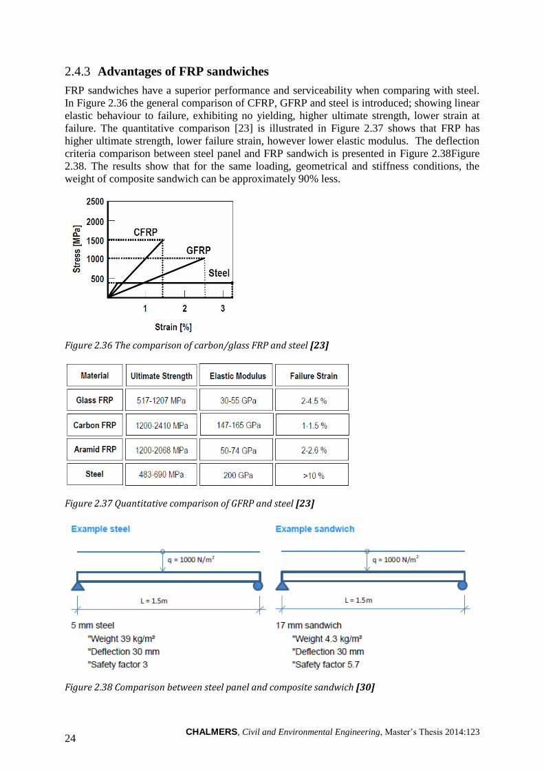
Composition of the study-case FRP sandwich panel 2.4.2
The sandwich structure analysed in this thesis consists of glass fibre, epoxy resin, and foam
core, bonded with epoxy adhesives. The promotion for choosing glass fibre from the variety
of fibres is that they are cheap and provide high strength. Moreover, structures containing
glass fibres are stiff, corrosion and impact resistant which is greatly important in the
application for culverts, due to constant exposition to severe environment and abrasion
sensibility. For the examined sandwich ―E‖ type glass fibres were tailored, because of their
high tensile strength and durability.
The epoxy resins suggest high workability and durability (Section Matrix constituents). Foam
core provides a well-performing structure due to greater interface between laminas and core
(Figure 2.35). In order to obtain a high-strength bond, sandwich is compounded with epoxy
adhesives.
Figure 2.35 Example of FRP sandwich with foam core [32]
CHALMERS, Civil and Environmental Engineering, Master’s Thesis 2014:123 24
Advantages of FRP sandwiches 2.4.3
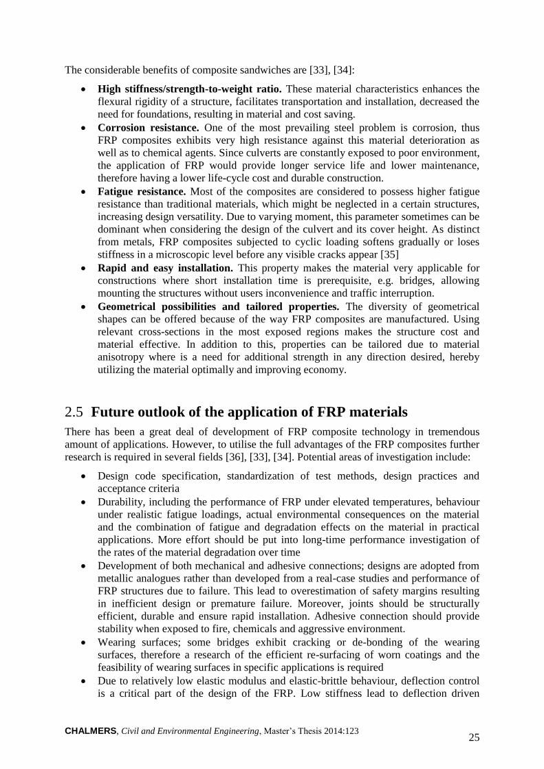
FRP sandwiches have a superior performance and serviceability when comparing with steel.
In Figure 2.36 the general comparison of CFRP, GFRP and steel is introduced; showing linear
elastic behaviour to failure, exhibiting no yielding, higher ultimate strength, lower strain at
failure. The quantitative comparison [23] is illustrated in Figure 2.37 shows that FRP has
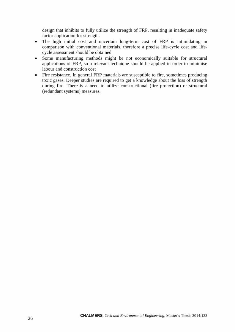
higher ultimate strength, lower failure strain, however lower elastic modulus. The deflection
criteria comparison between steel panel and FRP sandwich is presented in Figure 2.38Figure
2.38. The results show that for the same loading, geometrical and stiffness conditions, the
weight of composite sandwich can be approximately 90% less.
Figure 2.36 The comparison of carbon/glass FRP and steel [23]
Figure 2.37 Quantitative comparison of GFRP and steel [23]
Figure 2.38 Comparison between steel panel and composite sandwich [30]
CHALMERS, Civil and Environmental Engineering, Master’s Thesis 2014:123 25
The considerable benefits of composite sandwiches are [33], [34]:
High stiffness/strength-to-weight ratio. These material characteristics enhances the
flexural rigidity of a structure, facilitates transportation and installation, decreased the
need for foundations, resulting in material and cost saving.
Corrosion resistance. One of the most prevailing steel problem is corrosion, thus
FRP composites exhibits very high resistance against this material deterioration as
well as to chemical agents. Since culverts are constantly exposed to poor environment,
the application of FRP would provide longer service life and lower maintenance,
therefore having a lower life-cycle cost and durable construction.
Fatigue resistance. Most of the composites are considered to possess higher fatigue
resistance than traditional materials, which might be neglected in a certain structures,
increasing design versatility. Due to varying moment, this parameter sometimes can be
dominant when considering the design of the culvert and its cover height. As distinct
from metals, FRP composites subjected to cyclic loading softens gradually or loses
stiffness in a microscopic level before any visible cracks appear [35]
Rapid and easy installation. This property makes the material very applicable for
constructions where short installation time is prerequisite, e.g. bridges, allowing
mounting the structures without users inconvenience and traffic interruption.
Geometrical possibilities and tailored properties. The diversity of geometrical
shapes can be offered because of the way FRP composites are manufactured. Using
relevant cross-sections in the most exposed regions makes the structure cost and
material effective. In addition to this, properties can be tailored due to material
anisotropy where is a need for additional strength in any direction desired, hereby
utilizing the material optimally and improving economy.
Future outlook of the application of FRP materials 2.5
There has been a great deal of development of FRP composite technology in tremendous
amount of applications. However, to utilise the full advantages of the FRP composites further
research is required in several fields [36], [33], [34]. Potential areas of investigation include:
Design code specification, standardization of test methods, design practices and
acceptance criteria
Durability, including the performance of FRP under elevated temperatures, behaviour
under realistic fatigue loadings, actual environmental consequences on the material
and the combination of fatigue and degradation effects on the material in practical
applications. More effort should be put into long-time performance investigation of
the rates of the material degradation over time
Development of both mechanical and adhesive connections; designs are adopted from
metallic analogues rather than developed from a real-case studies and performance of
FRP structures due to failure. This lead to overestimation of safety margins resulting
in inefficient design or premature failure. Moreover, joints should be structurally
efficient, durable and ensure rapid installation. Adhesive connection should provide
stability when exposed to fire, chemicals and aggressive environment.
Wearing surfaces; some bridges exhibit cracking or de-bonding of the wearing
surfaces, therefore a research of the efficient re-surfacing of worn coatings and the
feasibility of wearing surfaces in specific applications is required
Due to relatively low elastic modulus and elastic-brittle behaviour, deflection control
is a critical part of the design of the FRP. Low stiffness lead to deflection driven
CHALMERS, Civil and Environmental Engineering, Master’s Thesis 2014:123 26
design that inhibits to fully utilize the strength of FRP, resulting in inadequate safety
factor application for strength.
The high initial cost and uncertain long-term cost of FRP is intimidating in
comparison with conventional materials, therefore a precise life-cycle cost and life-
cycle assessment should be obtained
Some manufacturing methods might be not economically suitable for structural
applications of FRP, so a relevant technique should be applied in order to minimise
labour and construction cost
Fire resistance. In general FRP materials are susceptible to fire, sometimes producing
toxic gases. Deeper studies are required to get a knowledge about the loss of strength
during fire. There is a need to utilize constructional (fire protection) or structural
(redundant systems) measures.

CHALMERS, Civil and Environmental Engineering, Master’s Thesis 2014:123 27
3 Design of Steel Culverts
Introduction 3.1
In this section culverts using corrugated steel plates are design for a collection of
representative cases. An analysis of the design results is performed to investigate the
governing issue that involved in the design of steel culverts, which helps to obtain a clear
picture about the primary problems that limit the application of steel culverts in practice.
The design reports of steel culverts can be found in the Appendix A.2. The Swedish Design
Method (SDM) [37]developed by Lars Pettersson and Håkan Sundquist is applied in the
design reports. Since it’s a design method that independent of codes [38], both Swedish
standards and European codes can be used in the verification. In this thesis relevant
Eurocodes are applied to the design process (see Table 3.1).
Table 3.1 Eurocodes used for the design of steel culverts
Issues Eurocodes
Loads and Materials EN 1990, EN 1991-2, EN 1993-1-1, EN 1993-2
Fatigue EN 1993-1-8, EN 1993-1-9
Design cases 3.2
In order to have a comprehensive understanding of steel culverts regarding mechanical
performance the primary task is to determine a reasonable and representative collection of the
design cases that culvert structures can be designed for. The conditions that control the choice
of design models includes: 1) culvert profile, 2) dimension of span and 3) height of the soil
cover.
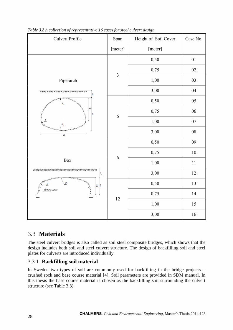
In the SDM manual seven types of culverts are introduced. The Profile E (Pipe-arch culvert)
and Profile G (Box culvert) are chosen for study. The Pipe-arch profile, also known as low-
rise profile, is one of the most commonly used types for the culvert bridges, while the box
culverts are preferred in long-span cases. The proper dimensions of span corresponding to
these two culvert profiles are determined (see Table 3.2).
The height of soil cover has substantial influence on the culvert structure. Four values—0.5
meter, 0.75 meter, 1.0 meter and 3.0 meter—are selected for the design cases. As introduced
in the SDM manual the minimum height of soil cover is 0.5 meter. A soil cover of 0.75-
meter- or 1.0-meter-height is commonly applied in the bridge culvert projects, and the 3-meter
soil represents the upper limit condition.
Based on the variables discussed 16 design cases in total are determined to carry on the design
of steel culverts (see Table 3.2).
CHALMERS, Civil and Environmental Engineering, Master’s Thesis 2014:123 28
Table 3.2 A collection of representative 16 cases for steel culvert design
Culvert Profile Span Height of Soil Cover Case No.
[meter] [meter]
Pipe-arch
3
0,50 01
0,75 02
1,00 03
3,00 04
6
0,50 05
0,75 06
1,00 07
3,00 08
Box
6
0,50 09
0,75 10
1,00 11
3,00 12
12
0,50 13
0,75 14
1,00 15
3,00 16
Materials 3.3
The steel culvert bridges is also called as soil steel composite bridges, which shows that the
design includes both soil and steel culvert structure. The design of backfilling soil and steel
plates for culverts are introduced individually.
Backfilling soil material 3.3.1
In Sweden two types of soil are commonly used for backfilling in the bridge projects—
crushed rock and base course material [4]. Soil parameters are provided in SDM manual. In
this thesis the base course material is chosen as the backfilling soil surrounding the culvert
structure (see Table 3.3).

CHALMERS, Civil and Environmental Engineering, Master’s Thesis 2014:123 29
Table 3.3 Soil parameters for base course backfilling material (Reference [37], Table B.2.1)
Fill material Optimum
density Density
Angel of
friction
Static soil
pressure Cu d50
kN/m3 kN/m
3
o K0 d60/d10 mm
Base course
material 20.6 20 40 0.36 10 20
Corrugated steel plates 3.3.2
Corrugations available on the market are normally given in such dimensions as shown in the
Table 3.4 below[37]. Steel plates of type 200*55 and type 380*140 are used for Pipe-arch
culverts and Box culvert respectively. In the design of box culverts, the crown and corner
sections usually become the most exposed regions. It is an economical way to apply the
reinforcing plate to increase the load-bearing capacity in certain sections (see Figure 3.1).
Table 3.4 Dimension of corrugated steel plates
Profile Type
[mm*mm]
c
[mm]
h.corr
[mm]
t
[mm]
125*26 125 26 1.5 – 4
150*50 150 50 2 – 7
200*55 200 55 2 – 7
380*140 380 140 4 – 7
Figure 3.1 Box culverts with reinforcement plates in crown and corner region
Reinforcement plates at corner Reinforcement plates at crown
CHALMERS, Civil and Environmental Engineering, Master’s Thesis 2014:123 30
Loads 3.4
Load effects from the surrounding soil 3.4.1
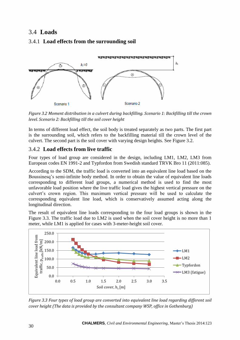
Figure 3.2 Moment distribution in a culvert during backfilling. Scenario 1: Backfilling till the crown
level. Scenario 2: Backfilling till the soil cover height
In terms of different load effect, the soil body is treated separately as two parts. The first part
is the surrounding soil, which refers to the backfilling material till the crown level of the
culvert. The second part is the soil cover with varying design heights. See Figure 3.2.
Load effects from live traffic 3.4.2
Four types of load group are considered in the design, including LM1, LM2, LM3 from
European codes EN 1991-2 and Typfordon from Swedish standard TRVK Bro 11 (2011:085).
According to the SDM, the traffic load is converted into an equivalent line load based on the
Boussinesq’s semi-infinite body method. In order to obtain the value of equivalent line loads
corresponding to different load groups, a numerical method is used to find the most
unfavorable load position where the live traffic load gives the highest vertical pressure on the
culvert’s crown region. This maximum vertical pressure will be used to calculate the
corresponding equivalent line load, which is conservatively assumed acting along the
longitudinal direction.
The result of equivalent line loads corresponding to the four load groups is shown in the
Figure 3.3. The traffic load due to LM2 is used when the soil cover height is no more than 1
meter, while LM1 is applied for cases with 3-meter-height soil cover.
Figure 3.3 Four types of load group are converted into equivalent line load regarding different soil
cover height (The data is provided by the consultant company WSP, office in Gothenburg)
0.0
50.0
100.0
150.0
200.0
250.0
0.0 0.5 1.0 1.5 2.0 2.5 3.0 3.5
Eq
uiv
alen
t li
ne
load
fro
m
traf
fic,
ptr
affi
c[k
N/m
]
Soil cover, hc [m]
LM1
LM2
Typfordon
LM3 (fatigue)

CHALMERS, Civil and Environmental Engineering, Master’s Thesis 2014:123 31
Verification and results 3.5
The capacity checks of the pipe-arch culvert have some minor difference with those of box
culverts. So, the verification list and final design results will be described separately. The
capacity of steel culverts are checked in the ultimate limit state (ULS) and the serviceability
state (SLS). Checks concerning fatigue are also performed, which can be regarded as a part of
the ultimate limit state checks. It is worthy to mention that the design cases with numbers in
red mean that the designed culvert structures cannot satisfy the requirements even though the
design parameters reach maximum values.
Case 01-08: Pipe-arch culvert 3.5.1
Verification
Table 3.5 Checks included in the verification of pipe-arch culverts
Culvert Profile Verification
Pipe-arch
Culvert
SLS Check 1: yielding in the upper section when backfilling till crown
Check 2: yielding in the upper section when soil cover completed
Check 3: Local buckling
ULS
Check 4: Plastic hinge in the crown, N & M
Check 5: Plastic hinge in the crown, N (M=0)
Check 6: Capacity in the bottom section
Check 7: Capacity of Bolts, shear stress
Check 8: Capacity of bolts, tensile stress
Check 9: Capacity of bolts, interaction
Fatigue
Check 10: Fatigue of the plate
Check 11: fatigue of Bolts, shear stress
Check 12: fatigue of Bolts, tensile stress
Check 13: fatigue of Bolts, interaction
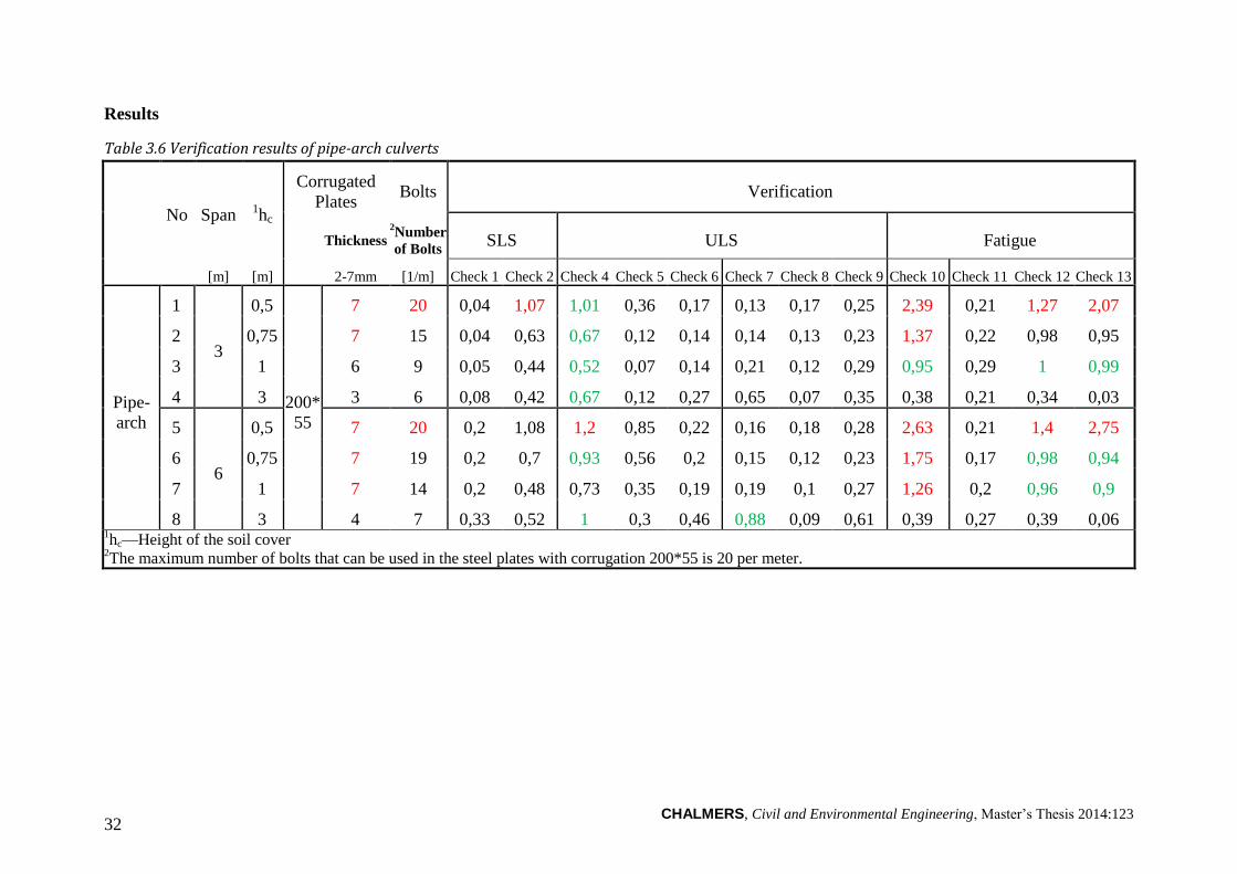
CHALMERS, Civil and Environmental Engineering, Master’s Thesis 2014:123 32
Results
Table 3.6 Verification results of pipe-arch culverts
No Span 1hc
Corrugated
Plates Bolts Verification
Thickness 2Number
of Bolts SLS ULS Fatigue
[m] [m] 2-7mm [1/m] Check 1 Check 2 Check 4 Check 5 Check 6 Check 7 Check 8 Check 9 Check 10 Check 11 Check 12 Check 13
Pipe-
arch
1
3
0,5
200*
55
7 20 0,04 1,07 1,01 0,36 0,17 0,13 0,17 0,25 2,39 0,21 1,27 2,07
2 0,75 7 15 0,04 0,63 0,67 0,12 0,14 0,14 0,13 0,23 1,37 0,22 0,98 0,95
3 1 6 9 0,05 0,44 0,52 0,07 0,14 0,21 0,12 0,29 0,95 0,29 1 0,99
4 3 3 6 0,08 0,42 0,67 0,12 0,27 0,65 0,07 0,35 0,38 0,21 0,34 0,03
5
6
0,5 7 20 0,2 1,08 1,2 0,85 0,22 0,16 0,18 0,28 2,63 0,21 1,4 2,75
6 0,75 7 19 0,2 0,7 0,93 0,56 0,2 0,15 0,12 0,23 1,75 0,17 0,98 0,94
7 1 7 14 0,2 0,48 0,73 0,35 0,19 0,19 0,1 0,27 1,26 0,2 0,96 0,9
8 3 4 7 0,33 0,52 1 0,3 0,46 0,88 0,09 0,61 0,39 0,27 0,39 0,06 1hc—Height of the soil cover
2The maximum number of bolts that can be used in the steel plates with corrugation 200*55 is 20 per meter.

CHALMERS, Civil and Environmental Engineering, Master’s Thesis 2014:123 33
Case 09-16: Box culvert 3.5.2
Verification
Table 3.7 Checks included in the verification of box culverts
Culvert Profile Verification
Box Culvert
SLS Check 1: yielding in the upper section when backfilling till crown
Check 2: yielding in the upper section when soil cover completed
Check 3: Local buckling
ULS
Check 4: Plastic hinge in the crown, N & M
Check 5: Plastic hinge in the crown, N (M=0)
Check 6: Plastic hinge in the corner, N & M
Check 7: Plastic hinge in the corner, N (M=0)
Check 8: Capacity of Bolts, shear stress
Check 9: Capacity of bolts, tensile stress
Check 10: Capacity of bolts, interaction
Fatigue
Check 11: Fatigue of the plate
Check 12: fatigue of Bolts, shear stress
Check 13: fatigue of Bolts, tensile stress
Check 14: fatigue of Bolts, interaction

CHALMERS, Civil and Environmental Engineering, Master’s Thesis 2014:123 34
Result
Table 3.8 Verification results of box culverts
No Span
1hc
Corrugated Plates Bolts Verification
Thickne
ss
2Reinf.
Top
Reinf.
Corner
3Number of
Bolts SLS ULS Fatigue
[m] [m]
4-7mm
[1/m]
Check
1
Check
2
Check
4
Check
5
Check
6
Check
7
Check
8
Check
9
Check
10
Check
11
Check
12
Check
13
Check
14
Box
9
6
0,50
380*
140
7 Yes No 15 0,05 0,51 0,99 0,74 0,73 0,13 0,21 0,55 0,61 1,11 0,28 3,95 61,47
10 0,75 5 Yes No 15 0,07 0,46 0,83 0,52 0,79 0,12 0,25 0,33 0,43 0,92 0,22 2,32 12,54
11 1,00 4 Yes No 15 0,08 0,42 0,73 0,41 0,86 0,13 0,29 0,23 0,34 0,76 0,19 1,55 3,69
12 3,00 7 No No 10 0,15 0,87 0,99 0,21 0,74 0,09 0,38 0,40 0,67 0,52 0,19 0,85 0,61
13
12
0,50 7 Yes No 15 0,04 0,56 1,59 1,16 0,87 0,19 0,28 0,57 0,69 1,05 0,28 3,74 52,38
14 0,75 7 Yes No 15 0,04 0,47 1,22 0,80 0,83 0,14 0,28 0,46 0,61 0,76 0,22 2,70 19,73
15 1,00 7 Yes No 15 0,04 0,43 1,02 0,63 0,84 0,12 0,29 0,41 0,58 0,59 0,19 2,12 9,51
16 3,00 7 Yes Yes 15 0,04 0,70 0,95 0,28 0,68 0,10 0,53 0,64 0,99 0,26 0,16 0,95 0,85
1hc—Height of the soil cover
2Reinf.—Reinforcement plates in the top region or corner region
3The maximum number of bolts that can be used in the steel plates with corrugation 380*140 is 15 per meter.

CHALMERS, Civil and Environmental Engineering, Master’s Thesis 2014:123 35
Summary and conclusions 3.6
The verification checks highlight the governing issue and limitations that involved
with steel culverts. In terms of the mechanical performance two major conclusions are
worthy to be mentioned:
1) Fatigue is the governing issue of steel culvert design. When the soil cover is no
more than one meter, the fatigue checks are dominant. In order to satisfy the fatigue
requirements the material utilization ratio is quite low.
2) Steel culverts are facing more challenges in the condition with large span. As
shown in the Box culvert design (Case 13-Case 15) not only fatigue but also capacity
of steel plates in ULS cannot be satisfied when the span increases to 12 meters.
The performance of steel culverts in terms of fatigue and strength gives high interest
to study the alternative using FRP materials, since the high fatigue-resistance and
strength are features of the FRP material.
Limitations and assumptions 3.7
As defined in the SDM manual in the section 3.3[37], the analysis of culvert is based
on the assumption that no special measures are applied during backfilling process. For
instance, adding soil on the pipe’s crown region during backfill is one method used to
reduce the crown rise. If this measure is applied, the calculation for forces and
moments need to be adapted.
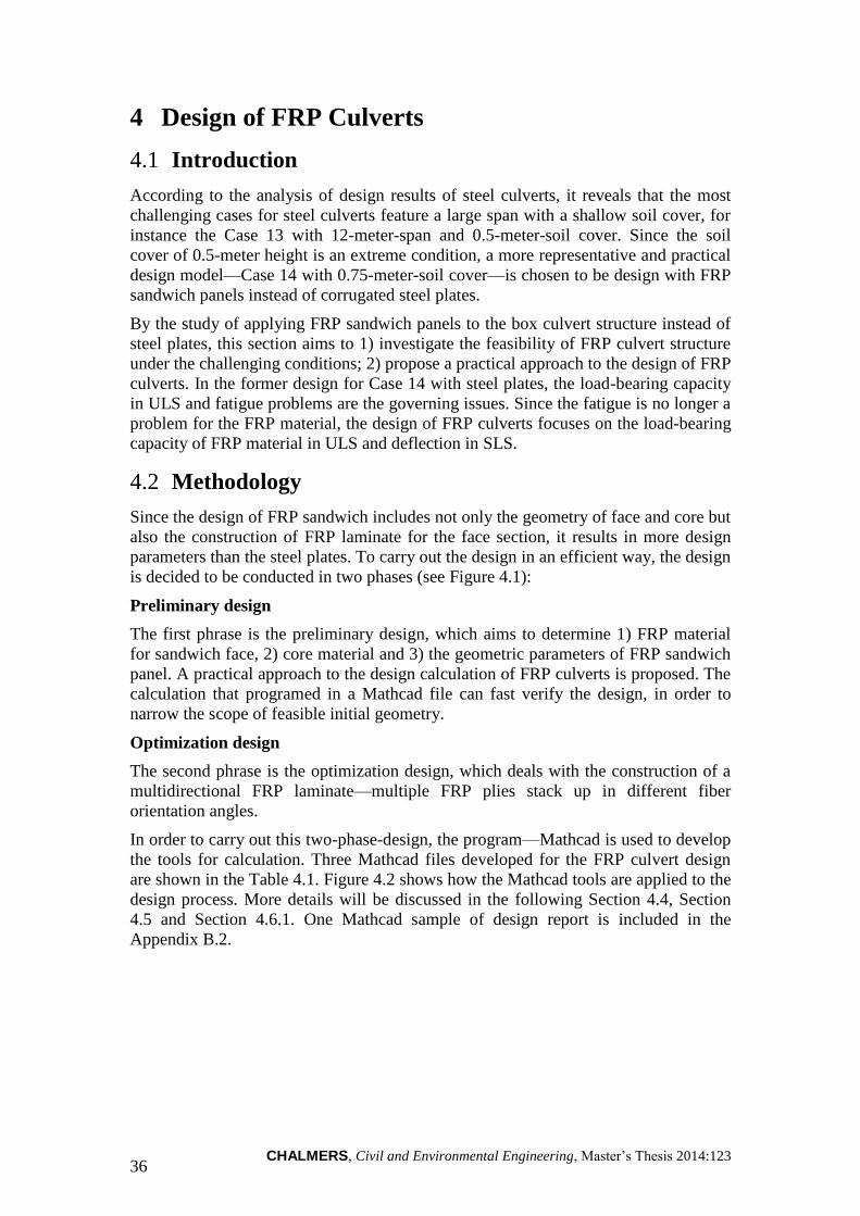
CHALMERS, Civil and Environmental Engineering, Master’s Thesis 2014:123 36
4 Design of FRP Culverts
Introduction 4.1
According to the analysis of design results of steel culverts, it reveals that the most
challenging cases for steel culverts feature a large span with a shallow soil cover, for
instance the Case 13 with 12-meter-span and 0.5-meter-soil cover. Since the soil
cover of 0.5-meter height is an extreme condition, a more representative and practical
design model—Case 14 with 0.75-meter-soil cover—is chosen to be design with FRP
sandwich panels instead of corrugated steel plates.
By the study of applying FRP sandwich panels to the box culvert structure instead of
steel plates, this section aims to 1) investigate the feasibility of FRP culvert structure
under the challenging conditions; 2) propose a practical approach to the design of FRP
culverts. In the former design for Case 14 with steel plates, the load-bearing capacity
in ULS and fatigue problems are the governing issues. Since the fatigue is no longer a
problem for the FRP material, the design of FRP culverts focuses on the load-bearing
capacity of FRP material in ULS and deflection in SLS.
Methodology 4.2
Since the design of FRP sandwich includes not only the geometry of face and core but
also the construction of FRP laminate for the face section, it results in more design
parameters than the steel plates. To carry out the design in an efficient way, the design
is decided to be conducted in two phases (see Figure 4.1):
Preliminary design
The first phrase is the preliminary design, which aims to determine 1) FRP material
for sandwich face, 2) core material and 3) the geometric parameters of FRP sandwich
panel. A practical approach to the design calculation of FRP culverts is proposed. The
calculation that programed in a Mathcad file can fast verify the design, in order to
narrow the scope of feasible initial geometry.
Optimization design
The second phrase is the optimization design, which deals with the construction of a
multidirectional FRP laminate—multiple FRP plies stack up in different fiber
orientation angles.
In order to carry out this two-phase-design, the program—Mathcad is used to develop
the tools for calculation. Three Mathcad files developed for the FRP culvert design
are shown in the Table 4.1. Figure 4.2 shows how the Mathcad tools are applied to the
design process. More details will be discussed in the following Section 4.4, Section
4.5 and Section 4.6.1. One Mathcad sample of design report is included in the
Appendix B.2.
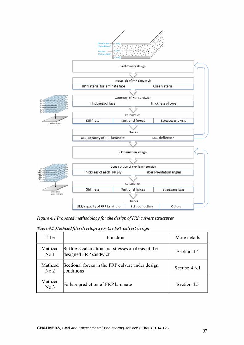
CHALMERS, Civil and Environmental Engineering, Master’s Thesis 2014:123 37
Figure 4.1 Proposed methodology for the design of FRP culvert structures
Table 4.1 Mathcad files developed for the FRP culvert design
Title Function More details
Mathcad
No.1
Stiffness calculation and stresses analysis of the
designed FRP sandwich Section 4.4
Mathcad
No.2
Sectional forces in the FRP culvert under design
conditions Section 4.6.1
Mathcad
No.3 Failure prediction of FRP laminate Section 4.5

CHALMERS, Civil and Environmental Engineering, Master’s Thesis 2014:123 38
Figure 4.2 Mathcad tools applied in the design process
Materials of the FRP sandwich panel 4.3
FRP laminate face 4.3.1
Ten commercial composites are listed in Reference [39] (Table A4-1). The fiber
reinforced composite E-glass—epoxy is chosen to construct the FRP laminate face of
sandwich panel. The physical and mechanical properties are shown in the Table 4.2.
Partial factors for FRP material are according to EUROCOMP Design Code [40]
shown in Table 4.3. In the preliminary design, all the FRP plies are stacking in the
same fiber orientation angle, which constructs a unidirectional FRP laminate with the
longitudinal direction parallel to the loading direction. In the optimization design, the
combinations of different fiber orientation angles are studied.
Table 4.2 Mechanical properties of chosen FRP material for initial design [39]
Material
Fiber
Volume
Fraction
Elastic Constants Strengths
𝐸11 𝐸22 𝑣12 𝐺12 𝜎11𝑡
𝜎11𝑐 𝜎22
𝑡 𝜎22𝑐 𝜏12
GPa GPa GPa MPa MPa MPa MPa MPa
E-glass &
Epoxy 45% 38.6 8.27 0.26 4.41 1062 610 31 118 72
Table 4.3 Partial factors for FRP material according to EUROCOMP Design Code [40]
Partial Factors for FRP material
γM1 γM2 γM3 γM=γM1*γM2*γM3
SLS 1,50 1,20 1,00 1,80
ULS 1,50 1,20 2,50 4,50
Design the FRP sandwich
Mathcad No. 1
Stiffness
Mathcad No. 2 Sectional forces
Mathcad No.1
for preliminary design
Mathcad No.3
for optimization design
Failure prediction
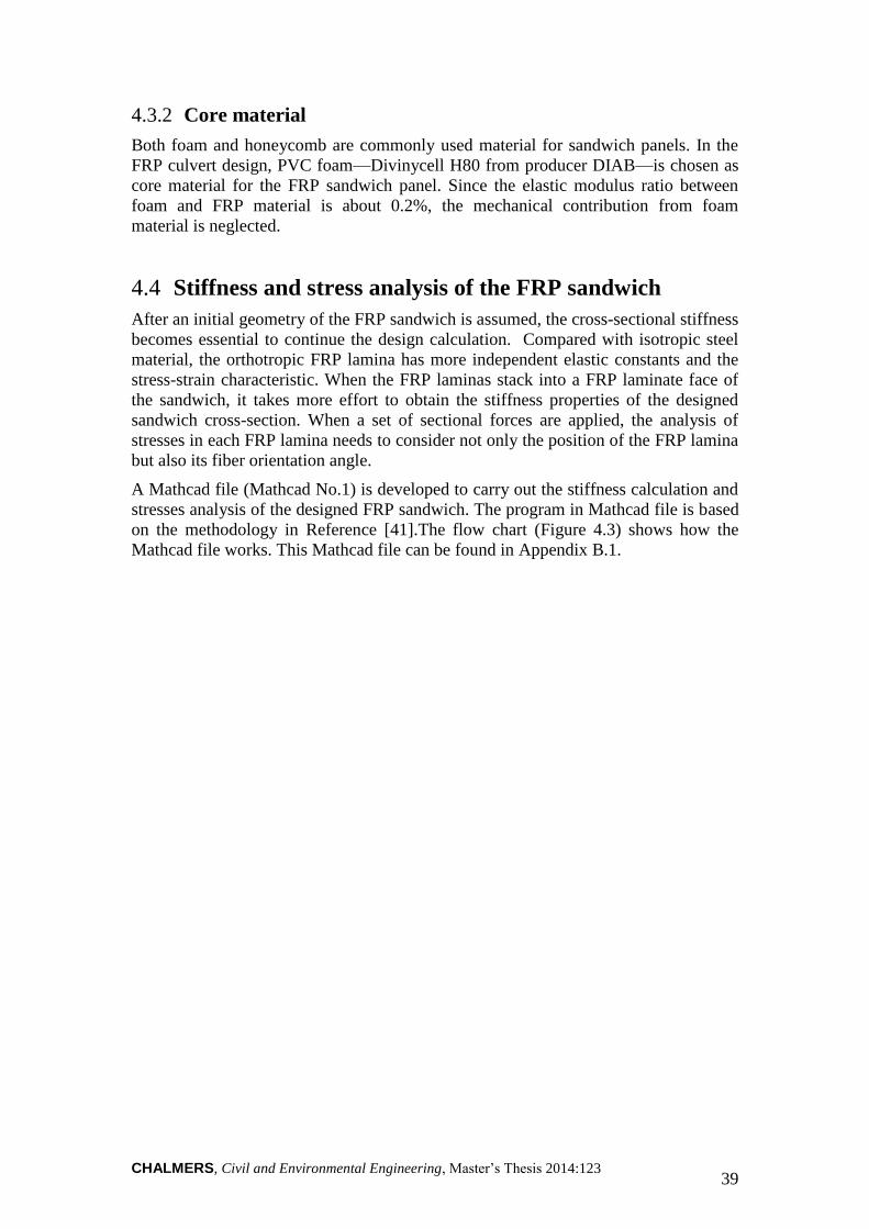
CHALMERS, Civil and Environmental Engineering, Master’s Thesis 2014:123 39
Core material 4.3.2
Both foam and honeycomb are commonly used material for sandwich panels. In the
FRP culvert design, PVC foam—Divinycell H80 from producer DIAB—is chosen as
core material for the FRP sandwich panel. Since the elastic modulus ratio between
foam and FRP material is about 0.2%, the mechanical contribution from foam
material is neglected.
Stiffness and stress analysis of the FRP sandwich 4.4
After an initial geometry of the FRP sandwich is assumed, the cross-sectional stiffness
becomes essential to continue the design calculation. Compared with isotropic steel
material, the orthotropic FRP lamina has more independent elastic constants and the
stress-strain characteristic. When the FRP laminas stack into a FRP laminate face of
the sandwich, it takes more effort to obtain the stiffness properties of the designed
sandwich cross-section. When a set of sectional forces are applied, the analysis of
stresses in each FRP lamina needs to consider not only the position of the FRP lamina
but also its fiber orientation angle.
A Mathcad file (Mathcad No.1) is developed to carry out the stiffness calculation and
stresses analysis of the designed FRP sandwich. The program in Mathcad file is based
on the methodology in Reference [41].The flow chart (Figure 4.3) shows how the
Mathcad file works. This Mathcad file can be found in Appendix B.1.

CHALMERS, Civil and Environmental Engineering, Master’s Thesis 2014:123 40
Figure 4.3 The flow chart shows how the Mathcad file functions to obtain the stiffness of
designed FRP sandwich and stresses for each FRP lamina
Failure prediction of FRP laminates 4.5
In the preliminary design phrase, the FRP laminate is constructed in a unidirectional
way. The stresses are linearly distributed according to the ply’s position. In these
cases, the first-ply-failure is applied, which means that the FRP laminate lose capacity
when the ply with maximum stresses fails. It can be performed in the Mathcad No.1
as shown in the Figure 4.2.
However, the first-ply-failure is too conservative to be used when it comes to the
optimization design with multi-directional FRP laminate. For a FRP laminate with a
combination of different fiber orientation angles, one ply fails does not necessarily
mean the laminate loses the load-bearing capacity. In order to predict the failure of a
FRP laminate in general, a Mathcad file (Mathcad No.3) is developed to perform the
prediction. The flow chart (Figure 4.4) below shows how the Mathcad program works.
The Mathcad No.3 can be found in Appendix B.3.

CHALMERS, Civil and Environmental Engineering, Master’s Thesis 2014:123 41
Figure 4.4 The flow chart shows how the Mathcad file functions to predict the failure of
multi-directional FRP laminate and obtain the equivalent strength
Sectional forces in FRP culverts 4.6
Besides the challenges discussed due to the orthotropic FRP material, the main task of
FRP culvert design is obtain the sectional forces in the FRP culvert structure. Since
the application of FRP material to the culvert structure is a newly proposed study
branch, no experience and design manual are available for guiding the FRP culvert
design. It becomes critical to figure out a practical approach to obtain the sectional
forces.
In the Swedish Design Method (SDM) for the steel culvert design, the original Soil
Culvert Interaction (SCI) method developed by Duncan (1977) is amended for the
calculation of sectional forces[4]. Inspired by the SDM, the calculation of FRP culvert
is determined to follow the amended SCI method in the SDM. The reliability of hand-
calculation results using SCI method will be discussed and then verified by FE-
modeling with Abaqus. A comparison of hand-calculation and FE-modeling results is
conducted to obtain the constructive suggestions for refining the hand-calculation
process.

CHALMERS, Civil and Environmental Engineering, Master’s Thesis 2014:123 42
Hand-calculation based on the SCI method 4.6.1
The Figure 4.5 shows the parameters used to calculate sectional forces by the
modified SCI method in the SDM manual. When FRP sandwich panels are used for
the culvert structure instead of steel plates, only the factor that represents the stiffness
of culvert wall needs to be modified to obtain normal forces and bending moments. A
Mathcad file (Mathcad No.2) is developed. A sample will be included in the
Appendix B.2.
Figure 4.5 Factors used to calculate sectional forces by the SCI method in the SDM manual
The Table 4.4 below shows the sectional forces in the FRP culvert by using SCI
method in the SDM. Case 14 is the design model, while case 15 is introduced as a
control design, which helps offer more data for comparison between hand-calculation
and FE-modeling results in the following sections. It reveals that the sectional forces
at the crown region in ULS get the maximum value when the backfilling till the soil
cover height.
Table 4.4 Sectional forces for the design case 14 and control case 15 calculated according
to the SCI method in the SDM
Results Senario 1
Backfilling till the crown
Senario 2
Backfilling till the soil cover height
SLS SLS ULS
N M_crown N M_crown N M_crown M_corner
kN/m kN*m/m kN/m kN*m/m kN/m kN*m/m kN*m/m
Case 14 -134,6 -3,7 -404,9 86,6 -546,6 118,3 48,4
Case 15 -134,6 -3,7 -418,5 78,0 -565,0 106,7 49,0
Reliability of hand-calculation 4.6.2
The SCI method in the SDM is amended for the steel culvert design and verified by
the in-site experiments. When it’s applied for the FRP culvert calculation, the
reliability of results needs to be analyzed and verified.
Since the calculation model in the SDM is two dimensional considering a unit strip of
the culvert, the stiffness of culvert wall as discussed in the Figure 4.5 is the stiffness
along the span direction. It means that the stiffness in the culvert’s longitudinal
direction is neglected. It’s acceptable for the steel culvert since the longitudinal
Sectional forces: N & M
Flexibility number
Stiffness of soil: Es
Stiffness of culvert wall:
EI
Design span of culvert: D
Geometry parameters
Geometry of culvert
structure
Geometry of surrounding soil
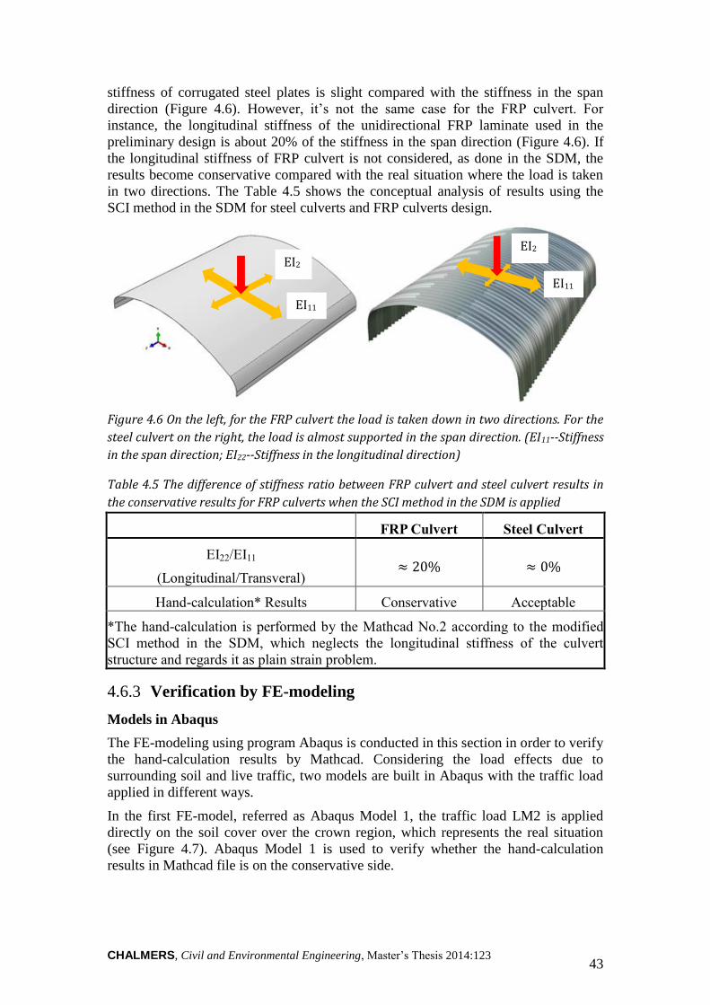
CHALMERS, Civil and Environmental Engineering, Master’s Thesis 2014:123 43
stiffness of corrugated steel plates is slight compared with the stiffness in the span
direction (Figure 4.6). However, it’s not the same case for the FRP culvert. For
instance, the longitudinal stiffness of the unidirectional FRP laminate used in the
preliminary design is about 20% of the stiffness in the span direction (Figure 4.6). If
the longitudinal stiffness of FRP culvert is not considered, as done in the SDM, the
results become conservative compared with the real situation where the load is taken
in two directions. The Table 4.5 shows the conceptual analysis of results using the
SCI method in the SDM for steel culverts and FRP culverts design.
Figure 4.6 On the left, for the FRP culvert the load is taken down in two directions. For the
steel culvert on the right, the load is almost supported in the span direction. (EI11--Stiffness
in the span direction; EI22--Stiffness in the longitudinal direction)
Table 4.5 The difference of stiffness ratio between FRP culvert and steel culvert results in
the conservative results for FRP culverts when the SCI method in the SDM is applied
FRP Culvert Steel Culvert
EI22/EI11
(Longitudinal/Transveral) ≈ 20% ≈ 0%
Hand-calculation* Results Conservative Acceptable
*The hand-calculation is performed by the Mathcad No.2 according to the modified
SCI method in the SDM, which neglects the longitudinal stiffness of the culvert
structure and regards it as plain strain problem.
Verification by FE-modeling 4.6.3
Models in Abaqus
The FE-modeling using program Abaqus is conducted in this section in order to verify
the hand-calculation results by Mathcad. Considering the load effects due to
surrounding soil and live traffic, two models are built in Abaqus with the traffic load
applied in different ways.
In the first FE-model, referred as Abaqus Model 1, the traffic load LM2 is applied
directly on the soil cover over the crown region, which represents the real situation
(see Figure 4.7). Abaqus Model 1 is used to verify whether the hand-calculation
results in Mathcad file is on the conservative side.
EI2
2
EI11
EI11
EI2
2
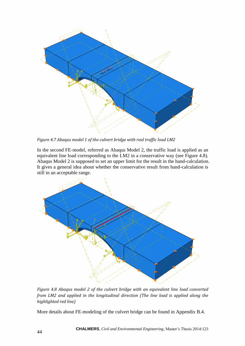
CHALMERS, Civil and Environmental Engineering, Master’s Thesis 2014:123 44
Figure 4.7 Abaqus model 1 of the culvert bridge with real traffic load LM2
In the second FE-model, referred as Abaqus Model 2, the traffic load is applied as an
equivalent line load corresponding to the LM2 in a conservative way (see Figure 4.8).
Abaqus Model 2 is supposed to set an upper limit for the result in the hand-calculation.
It gives a general idea about whether the conservative result from hand-calculation is
still in an acceptable range.
Figure 4.8 Abaqus model 2 of the culvert bridge with an equivalent line load converted
from LM2 and applied in the longitudinal direction (The line load is applied along the
highlighted red line)
More details about FE-modeling of the culvert bridge can be found in Appendix B.4.

CHALMERS, Civil and Environmental Engineering, Master’s Thesis 2014:123 45
Comparison of hand-calculation with FE-modeling results
The verification of hand-calculation by FE-modeling focuses on the sectional forces
in the crown region. Since the sectional forces are due to the surrounding soil and live
traffic, the results are analyzed separately, as shown in the Table 4.6Table 4.6 Both
the hand-calculation and FE-modeling are conducted for the control case 15, which is
used to see whether the difference of results varies in different conditions, for instance,
the soil cover height increases from 0.75 meter to 1.0 meter.
Table 4.6 Sectional forces for case 14 and case 15
Sectional
forces Case 14 Case 15 Comment
Crown Soil Traffic Soil Traffic
N M N M N M N M
Abaqus
Model 1
188,8 14,5 109,8 50,5 223,2 22 96,3 41 LM2
Hand-
calculation
327,3 27,1 219,4 91,3 390,6 40,4 174,4 69,3 SCI &
SDM
Abaqus
Model 2
188,8 14,5 270 162,4 223,2 22 207 121 Equivalent
LM2
The Figure 4.9 derived from the Table 4.6 shows the result ratio between hand-
calculation and FE-modeling. Based on the comparison, the following conclusion can
be drawn:
1) The hand-calculation is conservative. When the SCI method in the SDM is applied
directly to the FRP culvert design, the results from hand-calculation are greater than
those from Abaqus Model 1 which represents the real situation. It is valid no matter
when it comes to normal force or bending moment, soil load or traffic load, and case
14 or case 15.
2) The hand-calculation doesn’t exceed the upper limit. The sectional forces due to
traffic load in the hand-calculation are lower than the results from Abaqus Model 2.
Even though the initial hand-calculation results are on the conservative side, they are
still in an acceptable range. For preliminary design phrase, reduction factors can be
introduced to refine the initial hand-calculation.
3) Considering the sectional forces due to soil, the difference between hand-
calculation and FE-modeling keeps stable by comparing case 14 with case 15. As
discussed in the last section, the difference of results comes from the neglect of
longitudinal stiffness of FRP culvert in the SCI method.
4) Considering the sectional forces due to traffic, the ratio between Abaqus Model 1
and Hand-calculation varies from case 14 to case 15. The ratio increases from 50% to
55% for the normal force, and from 55% to 59% for the bending moment. Since the
different condition between case 14 and case 15 is the height of soil cover, it means
that not only the longitudinal stiffness but also the height of soil cover has influence
on the reliability of sectional forces due to traffic in the hand-calculation.
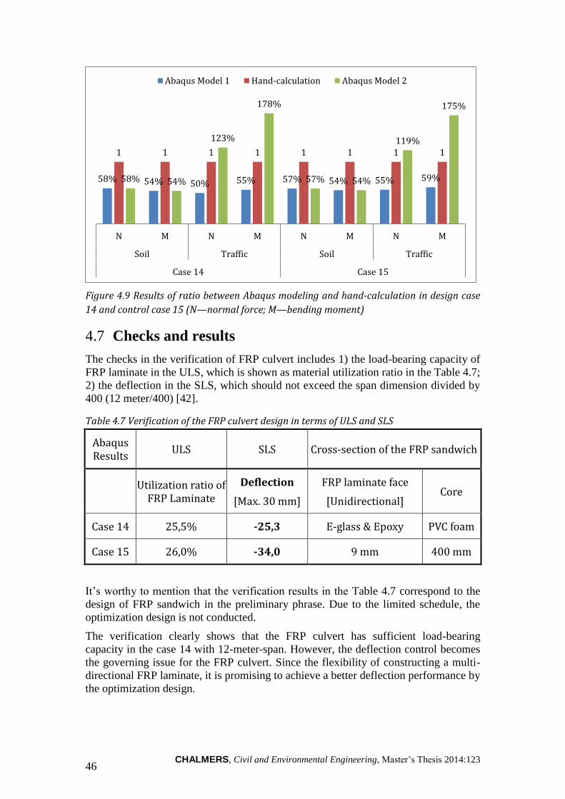
CHALMERS, Civil and Environmental Engineering, Master’s Thesis 2014:123 46
Figure 4.9 Results of ratio between Abaqus modeling and hand-calculation in design case
14 and control case 15 (N—normal force; M—bending moment)
Checks and results 4.7
The checks in the verification of FRP culvert includes 1) the load-bearing capacity of
FRP laminate in the ULS, which is shown as material utilization ratio in the Table 4.7;
2) the deflection in the SLS, which should not exceed the span dimension divided by
400 (12 meter/400) [42].
Table 4.7 Verification of the FRP culvert design in terms of ULS and SLS
Abaqus Results
ULS SLS Cross-section of the FRP sandwich
Utilization ratio of FRP Laminate
Deflection
[Max. 30 mm]
FRP laminate face
[Unidirectional] Core
Case 14 25,5% -25,3 E-glass & Epoxy PVC foam
Case 15 26,0% -34,0 9 mm 400 mm
It’s worthy to mention that the verification results in the Table 4.7 correspond to the
design of FRP sandwich in the preliminary phrase. Due to the limited schedule, the
optimization design is not conducted.
The verification clearly shows that the FRP culvert has sufficient load-bearing
capacity in the case 14 with 12-meter-span. However, the deflection control becomes
the governing issue for the FRP culvert. Since the flexibility of constructing a multi-
directional FRP laminate, it is promising to achieve a better deflection performance by
the optimization design.
58% 54% 50% 55% 57% 54% 55% 59%
1 1 1 1 1 1 1 1
58% 54%
123%
178%
57% 54%
119%
175%
N M N M N M N M
Soil Traffic Soil Traffic
Case 14 Case 15
Abaqus Model 1 Hand-calculation Abaqus Model 2
CHALMERS, Civil and Environmental Engineering, Master’s Thesis 2014:123 47
Summary and conclusions 4.8
Structural feasibility of FRP culverts 4.8.1
The design of FRP culvert in this chapter shows that issues of fatigue and load-
bearing capacity are not problems when FRP sandwich panels are applied to the
culvert structure instead of steel plates. In terms of the checks of FRP strength and
deflection, the verification shows that FRP culvert can succeed the challenges from
the design case 14. Since the deflection of FRP culverts becomes dominant, the design
of multi-directional FRP laminate in the optimization phrase is promising to have
good control of deflection.
Refine the proposed design method for FRP culverts 4.8.2
Based on the analysis of results and comparison, the hand-calculation of sectional
forces (performed by Mathcad No.2) is worthy to be refined. It will be further
discussed in the Section 6.2.1.

CHALMERS, Civil and Environmental Engineering, Master’s Thesis 2014:123 48
5 Life-cycle Cost Analysis
Introduction 5.1
Life cycle cost analysis is a technique to estimate the comparative cost of the assets
over the whole service-life or specific period of time by applying economic factors
[43]. Life-cycle cost phases which considerably influence the total LCC of the system
are represented in Figure 5.1. The life-cycle stages show that the total investment in
the project has a number of components that includes monetary means by the
consumption of material and energy.
Figure 5.1 Life-cycle cost phases [34]
Generally, life-cycle costs are divided into agency and social costs (Figure 5.2).
Agency costs include initial construction, operation and maintenance and disposal
costs, basically consisting of the analogous elements: material, transportation,
equipment and labour costs. The price for maintenance activities for inspection and
repair should be accounted for long-term issues, which might become even more
complex due to upraise of modern technologies and uncertainties for future
maintenance actions. Disposal costs appear at the end of service life of the asset. One
of the cost elements waste disposal can be even profitable, due to recyclable materials
such as steel or FRP. Social costs are mostly related to traffic and people, and are
divided into user and society costs. The cost units of user delay, vehicle operating and
accident are calculated by respective equations (Social costs). Environmental costs are
often taken into account by performing life-cycle assessment [2], [34].
Figure 5.2 Cost phases of life-cycle cost analysis [34]
Design and planning
Tendering Construction Operation & maintenance
End of service life
Total life-cycle cost
Agency costs
Initial construction
costs
Material costs
Transportation costs
Equipment costs
Labour costs
Operation & maintenance
costs
Material costs
Transportation costs
Equipment costs
Labour costs
Disposal costs
Waster disposal
Transportation costs
Equipment costs
Labour costs
Social costs
User costs
User delay costs
Vehicle operating costs
Society costs
Environmental costs
Accident costs

CHALMERS, Civil and Environmental Engineering, Master’s Thesis 2014:123 49
LCC analysis of the study-case 5.2
Purpose of LCC analysis 5.2.1
In this thesis life-cycle cost analysis is performed in order to show that FRP sandwich
is an economical solution for a culvert structure. The aim of the case study is not to
obtain the total investment, but to acquire the prices of the materials, structural
members itself and maintenance in order to show the monetary differences of two
alternatives.
Assumptions 5.2.2
To be consistent with the study, case 14 is chosen for further analysis, considering the
fact that this case can be applicable in reality, moreover having a big span of 12 meter,
therefore being challenging for steel. Additionally, two culverts are assumed to be
newly built as a road bridges and water passage under it. For the cost analysis the
following assumptions are made:
The costs in the design phase are excluded
Due to the scope of the thesis, construction site preparation, earthwork
(excavation, backfill), pavement and guard railing costs are omitted
Environmental issues are not considered in this thesis.
Accidental costs are disregarded due to lack of data.
Limitations 5.2.3
The life-span of the FRP culvert is assumed to be 100 years, while steel culvert has 80
years. In order to make a comparison the assumption of obsolescence is made,
therefore both culverts are demolished. The analysis assumed to be confined to such
boundaries:
The period of analysis is assumed to be from the manufacturing of the culvert
structural members until demolition
The costs that are included in the analysis: materials, manufacturing,
transportation, installation & construction, users, maintenance and demolition.
Agency costs 5.3
Initial construction costs 5.3.1
Initial costs include material, manufacturing, transportation and installation costs.
Aside user costs are considered due to road works during culvert erection and since it
is assumed a water passage via conduit, there is neither vehicle nor passenger traffic
interruption during maintenance.
Material costs
Steel culvert price include:
SuperCor SC-54 B corrugated panels
Crown and corner reinforcement plates
M 20 class 8.8 class
Protective layers: hot-dip galvanizing (according to EN ISO 1461) with an
average coat thickness 85 µm and extra epoxy painting with a thickness of 200
µm, covered from both sides 100 % perimeter
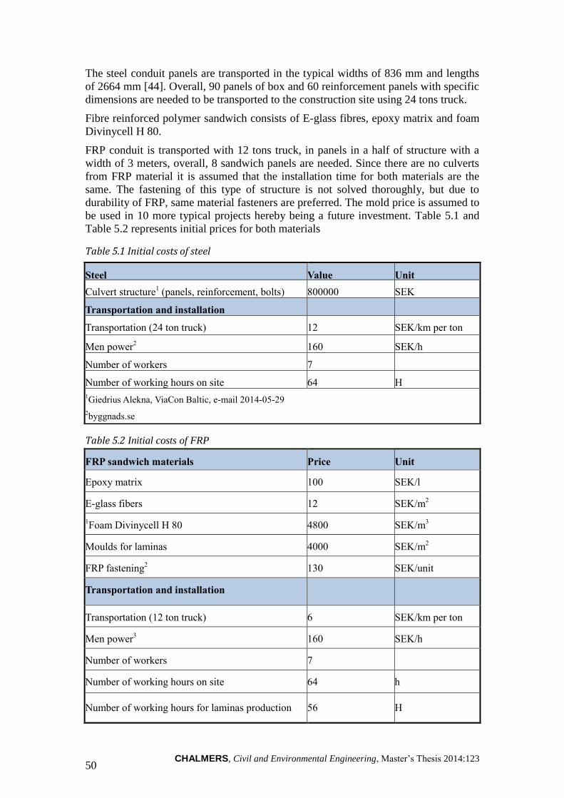
CHALMERS, Civil and Environmental Engineering, Master’s Thesis 2014:123 50
The steel conduit panels are transported in the typical widths of 836 mm and lengths
of 2664 mm [44]. Overall, 90 panels of box and 60 reinforcement panels with specific
dimensions are needed to be transported to the construction site using 24 tons truck.
Fibre reinforced polymer sandwich consists of E-glass fibres, epoxy matrix and foam
Divinycell H 80.
FRP conduit is transported with 12 tons truck, in panels in a half of structure with a
width of 3 meters, overall, 8 sandwich panels are needed. Since there are no culverts
from FRP material it is assumed that the installation time for both materials are the
same. The fastening of this type of structure is not solved thoroughly, but due to
durability of FRP, same material fasteners are preferred. The mold price is assumed to
be used in 10 more typical projects hereby being a future investment. Table 5.1 and
Table 5.2 represents initial prices for both materials
Table 5.1 Initial costs of steel
Table 5.2 Initial costs of FRP
FRP sandwich materials
Price Unit
Epoxy matrix
100 SEK/l
E-glass fibers
12 SEK/m2
1Foam Divinycell H 80
4800 SEK/m3
Moulds for laminas
4000 SEK/m2
FRP fastening2
130 SEK/unit
Transportation and installation
Transportation (12 ton truck) 6 SEK/km per ton
Men power3
160 SEK/h
Number of workers
7
Number of working hours on site
64 h
Number of working hours for laminas production 56 H
Steel
Value Unit
Culvert structure1 (panels, reinforcement, bolts)
painting)
800000 SEK
Transportation and installation
Transportation (24 ton truck) 12 SEK/km per ton
Men power2
160 SEK/h
Number of workers
7
Number of working hours on site
64 H
1Giedrius Alekna, ViaCon Baltic, e-mail 2014-05-29
2byggnads.se

CHALMERS, Civil and Environmental Engineering, Master’s Thesis 2014:123 51
1Anders Lindström, DIAB Sverige AB, e-mail 2014-05-28
2 cmcn.en.alibaba.com
3byggnads.se
Operation and maintenance costs 5.3.2
In order to find the total price of LCC the phase of operation and maintenance should
be thoroughly done. Due to deficiency of accurate data of specific maintenance
activities, an annual steel culvert maintenance price was adopter according to Safi,
2012. However, the maintenance activities that are done during the service life of steel
culvert usually are [45]:
Foundations. Check for erosion, cleavage, corrosion of reinforcement, flushing,
settlements, cracks, displacement
Slopes
Walls (inlets and outlets). Check for erosion, cleavage, corrosion of
reinforcement, cracks, deformation, displacement
Main bearing structure (conduit). Check for corrosion, cracks, protective layer,
change of conduit shape, displacement of the structure
Bolts. Check for corrosion, degradation, dissolve
Entire bridge. Check for vegetation, damping, scouring, debris, siltation
The major concern about the exploitation of steel culvert arise when maintaining a
sufficient protective layer against corrosion, therefore the culvert is assumed to be
repainted every 15 years.
The service life of FRP culvert can be taken as almost no maintenance, due to
resistance to the aggressive environment, which in study-case is water passing under
the culvert. Despite the durability of FRP the same general checks for obstruction or
maintaining other parts of the whole system are required, therefore the service-life
cost is taken into account as 10 % of steel maintenance cost.
In order to evaluate future investment a Net Present Value method (NPV) is used [2].
In this method a discount rate is used; the basic principle of discounting is that the
sum of money at hand at the present has a higher value than the same amount of
money in the future (Langdon, 2007). Discount rate computes future amount of
money into present value, taking into consideration inflation and the actual earning
power of money. All these future investments should be converted to the present
value with a discount rate of 3.5 % [46]. This can be done by using equation:
∑
( )
Where:
NPV=the life-cycle cost expressed as a present value;
n=the year considered;
Cn=sum of all cash flows in year n;
r=discount rate.
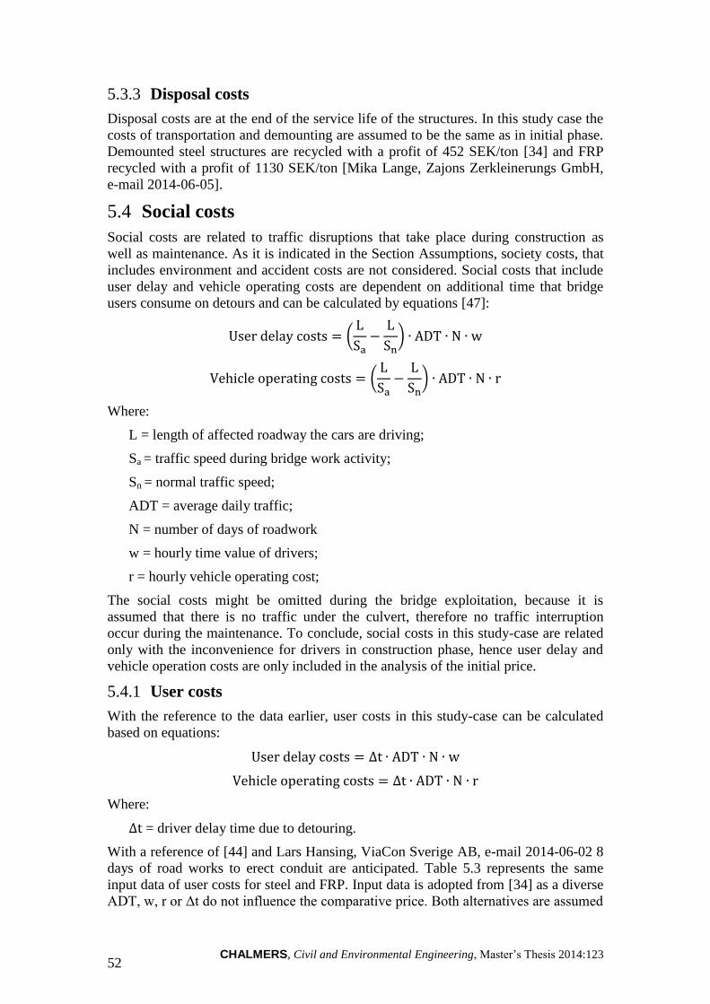
CHALMERS, Civil and Environmental Engineering, Master’s Thesis 2014:123 52
Disposal costs 5.3.3
Disposal costs are at the end of the service life of the structures. In this study case the
costs of transportation and demounting are assumed to be the same as in initial phase.
Demounted steel structures are recycled with a profit of 452 SEK/ton [34] and FRP
recycled with a profit of 1130 SEK/ton [Mika Lange, Zajons Zerkleinerungs GmbH,
e-mail 2014-06-05].
Social costs 5.4
Social costs are related to traffic disruptions that take place during construction as
well as maintenance. As it is indicated in the Section Assumptions, society costs, that
includes environment and accident costs are not considered. Social costs that include
user delay and vehicle operating costs are dependent on additional time that bridge
users consume on detours and can be calculated by equations [47]:
(
)
(
)
Where:
L = length of affected roadway the cars are driving;
Sa = traffic speed during bridge work activity;
Sn = normal traffic speed;
ADT = average daily traffic;
N = number of days of roadwork
w = hourly time value of drivers;
r = hourly vehicle operating cost;
The social costs might be omitted during the bridge exploitation, because it is
assumed that there is no traffic under the culvert, therefore no traffic interruption
occur during the maintenance. To conclude, social costs in this study-case are related
only with the inconvenience for drivers in construction phase, hence user delay and
vehicle operation costs are only included in the analysis of the initial price.
User costs 5.4.1
With the reference to the data earlier, user costs in this study-case can be calculated
based on equations:
Where:
= driver delay time due to detouring.
With a reference of [44] and Lars Hansing, ViaCon Sverige AB, e-mail 2014-06-02 8
days of road works to erect conduit are anticipated. Table 5.3 represents the same
input data of user costs for steel and FRP. Input data is adopted from [34] as a diverse
ADT, w, r or Δt do not influence the comparative price. Both alternatives are assumed

CHALMERS, Civil and Environmental Engineering, Master’s Thesis 2014:123 53
to have the same number of day of roadwork due to unknown installation time of FRP
culvert, even though it might be shorter considering the fact that it is only 8 panels to
be installed.
Table 5.3 User costs input data
Item Value Unit
Average daily traffic ADT1
796 Vehicle/day
Hourly time value of drivers1 w 254 SEK/h
Hourly vehicle operating cost1 r 187 SEK/h
Driver delay time due to detouring1 Δt, 15 min 0,25 h
Number of days of roadwork2 N 8 Days
1Mara V., 2014 [34]
2Lars Hansing, ViaCon Sverige AB, e-mail 2014-06-02, ViaCon brochure [44]
Results 5.5
Figure 5.3 represents the prices of all components that are considered in the analysis,
showing that material price for steel is about 30 % higher as well as 90 % more for
maintenance. Other elements prices such as installation, transportation, maintenance
and disposal are equal or nearly equal. The cost distribution in the initial phase is
shown in Figure 5.4 representing lower material cost of FRP in culvert structure.
Figure 5.3 Life-cycle cost comparison between steel and FRP
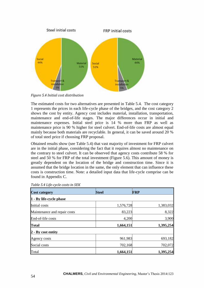
CHALMERS, Civil and Environmental Engineering, Master’s Thesis 2014:123 54
Figure 5.4 Initial cost distribution
The estimated costs for two alternatives are presented in Table 5.4. The cost category
1 represents the prices in each life-cycle phase of the bridges, and the cost category 2
shows the cost by entity. Agency cost includes material, installation, transportation,
maintenance and end-of-life stages. The major differences occur in initial and
maintenance expenses. Initial steel price is 14 % more than FRP as well as
maintenance price is 90 % higher for steel culvert. End-of-life costs are almost equal
mainly because both materials are recyclable. In general, it can be saved around 20 %
of total steel price if choosing FRP proposal.
Obtained results show (see Table 5.4) that vast majority of investment for FRP culvert
are in the initial phase, considering the fact that it requires almost no maintenance on
the contrary to steel culvert. It can be observed that agency costs contribute 58 % for
steel and 50 % for FRP of the total investment (Figure 5.6). This amount of money is
greatly dependent on the location of the bridge and construction time. Since it is
assumed that the bridge location in the same, the only element that can influence these
costs is construction time. Note: a detailed input data that life-cycle comprise can be
found in Appendix C.
Table 5.4 Life-cycle costs in SEK
Cost category Steel FRP
1 - By life-cycle phase
Initial costs 1,576,728 1,383,032
Maintenance and repair costs 83,223 8,322
End-of-life costs 4,200 3,900
Total 1,664,151 1,395,254
2 - By cost entity
Agency costs 961,983 693,182
Social costs 702,168 702,072
Total 1,664,151 1,395,254

CHALMERS, Civil and Environmental Engineering, Master’s Thesis 2014:123 55
Figure 5.5 Total life-cycle cost by life-cycle phase
Figure 5.6 Life-cycle cost by cost entity
Summary 5.6
As a summary of the life-cycle cost analysis it can be concluded that FRP culvert is
more economical alternative due to lower initial material and maintenance costs. It is
durable solution as well, regarding FRP material as not susceptible to aggressive
environment as distinct from steel material. In addition to this, the possibility to
recycle FRP makes it considerably sustainable material. Lastly, in the particular
study-case 14, an estimated FRP culvert is approximately 50 % lighter than steel
culvert, possessing cheaper transportation and installation price as well as faster
erection.

CHALMERS, Civil and Environmental Engineering, Master’s Thesis 2014:123 56
6 Conclusions
About FRP culvert structure 6.1
The study of applying FRP material in the culvert structure shows that the FRP
culvert is a promising alternative to the traditional steel culvert in the design of
challenging case.
Mechanical performance
The FRP culvert has better mechanical performance than the steel one in terms of
load-bearing capacity and fatigue issues. The study of case 14 shows that the FRP
culvert succeeds the challenges of large span and shallow soil cover, which cannot be
satisfied by using steel plates.
LCC analysis
The LCC analysis shows that the FRP culvert is also an economical alternative. The
application of FRP material gives culvert structure more durable and sustainable
performance in the service life.
Suggestions for future study 6.2
Proposed design method for FRP culvert 6.2.1
The proposed methodology for FRP culvert design as discussed in the chapter 4 needs
to be improved in the future study.
Calculation of sectional forces
In the preliminary design, the calculation of sectional forces for the FRP culvert
follows the amended SCI method in the SDM for steel culvert design. The verification
by FE-modeling proves that the results are conservative, and it’s valuable to refine the
hand-calculation method by introducing reduction factors. Based on the comparison in
the section 4.6, the following comments about reduction factors can be made.
The reduction factor for sectional forces due to soil is highly dependent on the
stiffness ratio between longitudinal and transversal.
The reduction factor for sectional forces due to traffic load is a function of
both stiffness ratio and height of soil cover.
In order to obtain the functions for determining the value of reduction factors in
different design conditions, more study cases by FE-modeling are required.
Verification of the FRP culvert structure
The verification of FRP culverts in this thesis includes the checks for load-bearing
capacity of FRP laminate in the ultimate limit state and deflection in the serviceability
limit state. In the future study more issues need to be considered in the design of FRP
culverts.
Capacity of core material
Capacity of the interfacial connection between core and FRP face
Design of connection details for FRP sandwich panels
Creep of FRP material

CHALMERS, Civil and Environmental Engineering, Master’s Thesis 2014:123 57
Applicability of FRP culverts 6.2.2
In this thesis, the FRP culvert is designed and compared with steel culverts only for
the selected challenging case 14 with 12-meter-span and 0.75-meter-soil cover. It’s
important to know whether the FRP culvert is still a competitive alternative when it
comes to smaller spans, for instance. In order to investigate the applicability of FRP
culverts, more comprehensive comparisons between steel and FRP culverts in
different conditions are needed in the future research.
Other materials for FRP culverts 6.2.3
The design of FRP sandwich chooses PVC foam as core material. Since the elastic
modulus of FRP material is much smaller than that of steel, it requires a large
thickness of core section in order to get a proper stiffness. The fact motivates the
study of honeycomb as core material instead of PVC foam in the future.
For the FRP laminate face, the epoxy matrix reinforced by E-glass fibers is chosen as
the FRP material in the FRP culvert design. Other types of FRP material, for example,
reinforced by G-glass or carbon fibers can also be applied if higher mechanical
properties are required.
Life-cycle assessment in the LCC analysis 6.2.4
In order to get more precise service life costs of culverts, maintenance activities for
both structures should be thoroughly analysed. Extraordinary attention should be paid
to long-term behaviour of FRP material, due to lack of practical examples of
underground structures. Moreover, since environmental issues nowadays becomes
more and more important, an influence of exhaust fumes during material
manufacturing, transportation, installation, maintenance and demolition should be
taken into account. One of the ways to do that is to perform life-cycle assessment.
After the evaluation of environmental impacts, a more evident conclusion could be
drawn about life-cycle cost of the structures.
CHALMERS, Civil and Environmental Engineering, Master’s Thesis 2014:123 58
7 References
[1] L. Pettersson and H. Sundquist, ―Design of Soil Steel Composite Bridges,‖
Stockholm, 2010.
[2] M. Safi, ―LCC Applications for Bridges and Integration with BMS,‖ KTH
Royal Institute of Technology, Stockholm, 2012.
[3] H. Sundquist, ―Soil-Steel Structures. State-of-the-art. Swedish Research.
Presentation in NordBalt Seminar,‖ 2007.
[4] L. Petterson, ―Full Scale Tests and Structural Evaluation of Soil Steel Flexible
Culverts with Low Height of Cover,‖ KTH, 2007.
[5] ―Components of the Culvert.‖ [Online]. Available:
http://www.cjntech.co.nz/manuals/Find the Answer/#2864.htm.
[6] ―Culverts.‖ [Online]. Available:
http://water.epa.gov/polwaste/nps/urban/upload/2003_07_24_NPS_unpavedroa
ds_ch3.pdf.
[7] J. F. Levine, C. B. Eads, W. G. Cope, L. F. Humphries, R. B. Bringolf, P. R.
Lazaro, D. Shea, J. Vander Pluym, D. Eggleston, M. A. Merril, J. Gregory, and
A. E. Bogan, ―Final Report Submitted To: North Carolina Department of
Transportation ( Project Number : HWY-2004-08 ) January 2007 Prepared By :
Technical Report Documentation Page,‖ 2007.
[8] U. University, ―Culvert Rehabilitation Practices,‖ Utah.
[9] ―Snap-Tite Large Diameter Culvert Lining Systems.‖ [Online]. Available:
http://www.culvert-rehab.com/pdfs/big-idea.pdf.
[10] ―Culvert Rehabilitation Systems.‖ [Online]. Available:
http://www.kenway.com/products/culvert-rehabilitation-systems/.
[11] ―Steel Culvert Re-lining.‖ [Online]. Available: http://www.eng.buffalo.edu/.
[12] ―Fiberglass Digester Domes.‖ [Online]. Available:
http://www.mekco.com/fiberglass_digester.htm.
[13] ―Mondial House.‖ [Online]. Available:
http://www.lightstraw.co.uk/ate/main/mondial/.
[14] ―Fiberline Composites.‖ [Online]. Available: http://www.fiberline.com/.
[15] ―Dawlish Railway station.‖ [Online]. Available:
http://www.reinforcedplastics.com/view/29001/steel-footbridge-replaced-with-
composite-at-uk-railway-station/.

CHALMERS, Civil and Environmental Engineering, Master’s Thesis 2014:123 59
[16] ―Dawlish FRP Railway Station.‖ [Online]. Available:
http://www.tech.plym.ac.uk/sme/composites/bridges.htm#dawlish.
[17] ―Corrosion Fluid Products Corp.‖ [Online]. Available:
http://corrosionfluid.com/.
[18] ―Plastics Pipe Institute.‖ [Online]. Available: https://plasticpipe.org/about-
ppi.html.
[19] ―Fiberglass pipe.‖ [Online]. Available: http://www.gwhaley.com/FRPPipe.htm.
[20] ―Composites.‖ [Online]. Available:
http://www.plasticoncomposites.com/en/composites.
[21] ―FRP composites.‖ [Online]. Available: http://reichhold.com/.
[22] M. Zoghi, The International Handbook of FRP Composites in Civil
Engineering. CRC Press, 2013, p. 706.
[23] I. E. Comittee, ―An Introduction to FRP Composites for Construction,‖ 2006.
[24] ―FRP Pipe Technologies.‖ [Online]. Available: http://www.pipemedic.com/.
[25] ―ABC’s of FRP Materials.‖ [Online]. Available:
http://www.autocomposites.org/composites101/abc.cfm.
[26] R. G. Weatherhead, FRP Technology: Fibre Reinforced Resin Systems. Applied
Science, 1980, p. 462.
[27] M. F. G. Companies, ―Technical Design Guide for FRP Composite Products
And Parts.‖
[28] M. V. Hosur, M. Abdullah, and S. Jeelani, ―Manufacturing and Low-Velocity
Impact Characterization of Foam Filled 3-D Integrated Core Sandwich
Composites with Hybrid Face Sheets,‖ Compos. Struct., vol. 69, no. 2, pp. 167–
181, Jul. 2005.
[29] E. M. Reis, ―Characteristics of Innovative 3-D FRP Sandwich Panels,‖ 2005.
[30] ―DIAB guide to core and sandwich,‖ Laholm, 2012.
[31] ―Core Materials: Nomex Honeycomb.‖ [Online]. Available:
http://www.fibermaxcomposites.com/shop/nomex-aramid-
honeycombbrthickness-mmbrcell-size-32-mm-p-647.html?cPath=77.
[32] ―Core materials: XPS foam.‖ [Online]. Available: http://www.cs-
jy.com/en/News/products-show.asp?cataid=000200020003.
[33] ―Current Practices in FRP Composites Technology.‖ [Online]. Available:
http://www.fhwa.dot.gov/bridge/frp/deckprac.cfm.

CHALMERS, Civil and Environmental Engineering, Master’s Thesis 2014:123 60
[34] V. Mara, ―Fibre reinforced polymer bridge decks : Sustainability and a novel
panel-level connection,‖ Chalmers University of Technology, 2014.
[35] P. B. Potyrala, ―Use of Fiber Reinforced Polymer Composites in Bridge
Construction. State of the Art in Hybrid and All-Composite Structures,‖
Technical University of Catalonia, 2011.
[36] T. A. Hoffard and L. J. Malvar, ―Fiber-Reinforced Polymer Composites in
Bridges: A State-of-the-Art Report,‖ 2005.
[37] L. Pettersson and H. Sundquist, ―Design of soil steel composite bridges,‖ 2009.
[38] A. H. H. Wadi, Soil steel composite bridges. 2012.
[39] B. D. Agarwal, L. J. Broutman, and K. Chandrashekhara, Analysis and
Performance of Fiber Composites. Wiley, 2006.
[40] J. L. Clarke, Structural Design of Polymer Composites: Eurocomp Design
Code and Background Document. Taylor & Francis, 2003.
[41] P. K. Mallick, Fiber-reinforced composites: materials, manufacturing, and
design. CRC Press, 2008.
[42] Guide Specifications for Design of FRP Pedestrian Bridges, 1st Edition.
American Association of State Highway and Transportation Officials, 2008.
[43] ―ETSI Project. Bridge Life Cycle Optimisation. Stage 3,‖ 2013.
[44] ViaCon, ―Burried Flexible Steel Structures SuperCor.‖
[45] Vägverket, ―BaTMan – Mätning och bedömning av broars tillstånd,‖ 2008.
[46] Trafikverket, ―Samhällsekonomiska principer och kalkylvärden för
transportsektorn: ASEK 5.1. Kapitel 3 Kalkylprinciper och generella
kalkylvärden,‖ 2014.
[47] M. A. EHLEN, ―Life-Cycle Costs of Fiber-Reinforced-Polymer Bridge Decks,‖
J. Mater. Civ. Eng., vol. 11, pp. 224–230, 1999.

CHALMERS, Civil and Environmental Engineering, Master’s Thesis 2014:123 61
8 Appendices
The appendices are list below:
Appendix A.1 Equivalent traffic line loads
Appendix A.2 Mathcad routine for design of corrugated steel culverts
Mathcad sample of Case 14
Appendix B.1 Mathcad routine for design of FRP culverts—Mathcad No.1
Stiffness calculation and stress analysis
Appendix B.2 Mathcad routine for design of FRP culverts—Mathcad No.2
Calculation of sectional forces
Appendix B.3 Mathcad routine for design of FRP culverts—Mathcad No.3
Failure prediction of the FRP laminate
Appendix B.4 Data for the FE analysis of FRP culverts in ABAQUS
Appendix C Data for LCC analysis

CHALMERS, Civil and Environmental Engineering, Master’s Thesis 2014:123 A1‐1
Appendix A.1 Equivalent line load due to live traffic The data of equivalent line load converted from four traffic groups in different soil cover conditions are provided by the supervisor Kristoffer Karlssen from the consultant company WSP at Gothenburg.
Table A.1‐1 Equivalent line load converted from traffic groups in varying soil coverconditions
Equivalent line load due to live traffic
Height of Soil Cover 0,5 0,6 0,7 0,8 0,9 1,0 1,3 1,5 2,0 2,5 3,0
LM1 165,3 151,6141,3134,3129,9127,7128,6133,4134,4 130,5 125,3
LM2 213,7 190,6170,8154,2140,5129,2108,4 94,9 80,3 74,2 68,9
Typfordon 156,5 139,6127,8119,2112,3110,5110,4106,9 95,6 88,6 89,4
LM3 (fatigue) 72,1 65,1 59,3 54,8 51,5 49,0 45,8 45,3 44,5 44,2 42,6
Figure A.1‐1 Equivalent line load converted from traffic groups in varying soil coverconditions
0.0
50.0
100.0
150.0
200.0
250.0
0.0 1.0 2.0 3.0 4.0
Equivalentlineloadfrom
traffic,
p traffic[kN/m
]
Heightofsoilcover,hc[m]
LM1
LM2
Typfordon
LM3(fatigue)
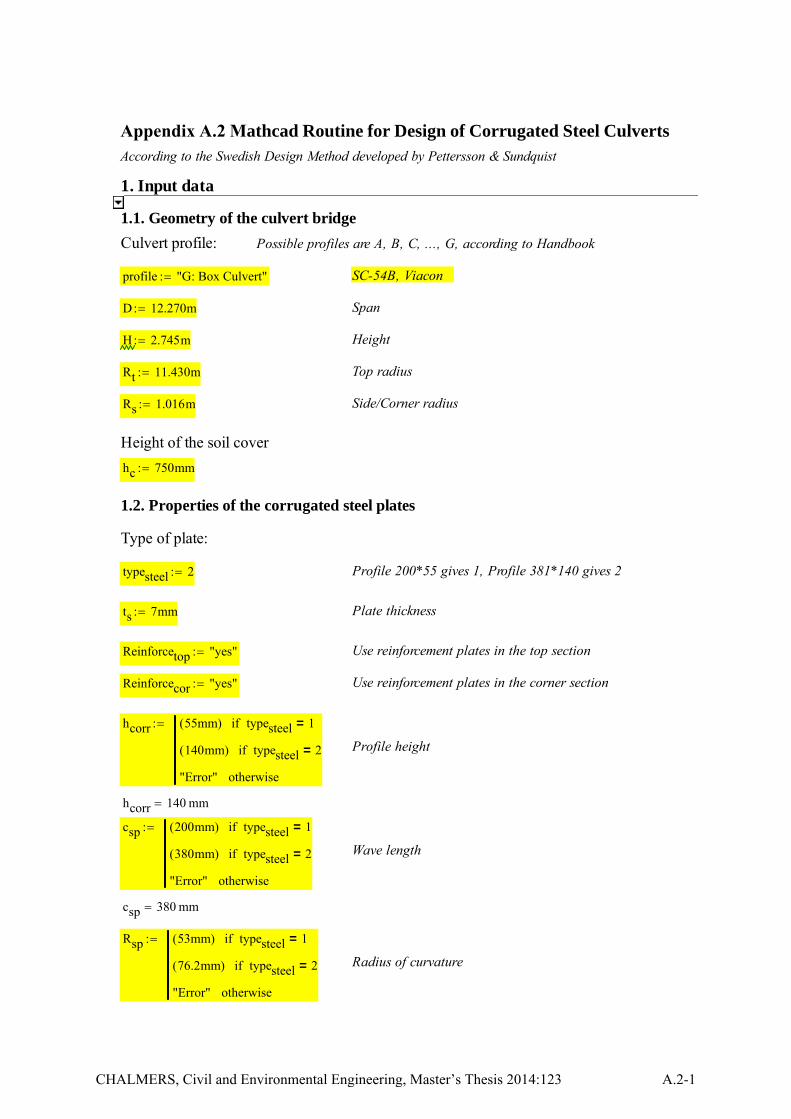
Appendix A.2 Mathcad Routine for Design of Corrugated Steel Culverts According to the Swedish Design Method developed by Pettersson & Sundquist
1. Input data
1.1. Geometry of the culvert bridge
Culvert profile: Possible profiles are A, B, C, ..., G, according to Handbook
profile "G: Box Culvert" SC-54B, Viacon
D 12.270m Span
H 2.745m Height
Rt 11.430m Top radius
Rs 1.016m Side/Corner radius
Height of the soil cover
hc 750mm
1.2. Properties of the corrugated steel plates
Type of plate:
typesteel 2 Profile 200*55 gives 1, Profile 381*140 gives 2
ts 7mm Plate thickness
Reinforcetop "yes" Use reinforcement plates in the top section
Reinforcecor "yes" Use reinforcement plates in the corner section
hcorr 55mm( ) typesteel 1=if
140mm( ) typesteel 2=if
"Error" otherwise
Profile height
hcorr 140 mm
csp 200mm( ) typesteel 1=if
380mm( ) typesteel 2=if
"Error" otherwise
Wave length
csp 380 mm
Rsp 53mm( ) typesteel 1=if
76.2mm( ) typesteel 2=if
"Error" otherwise
Radius of curvature
CHALMERS, Civil and Environmental Engineering, Master’s Thesis 2014:123 A.2-1

Rsp 76.2 mm
Steel grade S 315MC The SuperCor produced by Viacon conformsto EN 10149-2 or EN 10025-2
fyk 315MPa
fuk 470MPa
Es 210GPa
1.3. Parameters of the bolted connection
Bolts M20 class 8.8, EN ISO 898-1
fub 800MPa
fyb 640MPa
dbolt 20mm
Aboltπ
4dbolt
2 314.159 mm
2
nbolt15
m
abolt 100mm( ) typesteel 1=if
190mm( ) typesteel 2=if
"Error" otherwise
Distance between parallel rows (center to center)
1.4. Parameters of the backfilling soil
Type of the backfilling soil:
Base course material Parameters of soil taken from Appendix 2 of Handbook
ρopt 20.6kN
m3
Optium density
RP 97 Degree of compaction (%), standard proctor method
ρcvRP
100ρopt ρcv 19.982
kN
m3
ρ1 ρcv Density of the soil up to the height of the crown
ρ2 ρcv Mean density of the soil material with the region (hc+H/2)
Partical size distribution
d50 20mm d60 30mm d10 3mm
A.2-2 CHALMERS, Civil and Environmental Engineering, Master’s Thesis 2014:123
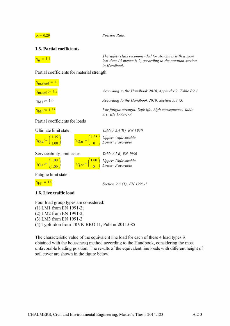
ν 0.29 Poisson Ratio
1.5. Partial coefficients
The safety class recommended for structures with a spanless than 15 meters is 2, according to the natation sectionin Handbook.
γn 1.1
Partial coefficients for material strength
γm.steel 1.1
γm.soil 1.3 According to the Handbook 2010, Appendix 2, Table B2.1
γM1 1.0 According to the Handbook 2010, Section 5.3 (3)
γMf 1.35 For fatigue strength: Safe life, high consequence, Table3.1, EN 1993-1-9
Partial coefficients for loads
Ultimate limit state: Table A2.4(B), EN 1990
Upper: UnfavorableLower: FavorableγG.u
1.35
1.00
γQ.u1.35
0
Serviceability limit state: Table A2.6, EN 1990
Upper: UnfavorableLower: FavorableγG.s
1.00
1.00
γQ.s1.00
0
Fatigue limit state:
γFf 1.0 Section 9.3 (1), EN 1993-2
1.6. Live traffic load
Four load group types are considered: (1) LM1 from EN 1991-2;(2) LM2 from EN 1991-2;(3) LM3 from EN 1991-2(4) Typfordon from TRVK BRO 11, Publ nr 2011:085
The characteristic value of the equivalent line load for each of these 4 load types isobtained with the boussinesq method according to the Handbook, considering the mostunfavorable loading position. The results of the equivalent line loads with different height ofsoil cover are shown in the figure below.
CHALMERS, Civil and Environmental Engineering, Master’s Thesis 2014:123 A.2-3
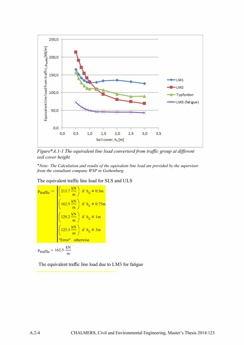
Figure*A.1-1 The equivalent line load converterd from traffic group at different soil cover height*Note: The Calculation and results of the equivalent line load are provided by the supervisorfrom the consultant company WSP in Gothenburg
The equivalent traffic line load for SLS and ULS
ptraffic 213.7kN
m
hc 0.5m=if
162.5kN
m
hc 0.75m=if
129.2kN
m
hc 1m=if
125.3kN
m
hc 3m=if
"Error" otherwise
ptraffic 162.5kN
m
The equivalent traffic line load due to LM3 for fatigue
A.2-4 CHALMERS, Civil and Environmental Engineering, Master’s Thesis 2014:123

ptraffic.fatigue 72.1kN
m
hc 0.5m=if
57.1kN
m
hc 0.75m=if
49.0kN
m
hc 1m=if
42.6kN
m
hc 3m=if
"Error" otherwise
ptraffic.fatigue 57.1kN
m
2. Calculation
2.1. Soil tangent modulus
Determination of relevant factors
ρs 26kN
m3
True density of the soil material, Appendix 2, Handbook
e1
ρs
ρ11 0.301 Void ratio
Cu
d60
d1010 Uniformity coefficient
m1 282 Cu0.77
e12.83
1.43 103
Modulus ratio
β 0.29 logd50
0.01mm
0.065 log Cu 0.892 Stress exponent
ϕk 26deg 10degRP 75( )
25 0.4deg Cu 1.6deg log
d50
1mm
ϕk 40.882 deg Characteristic angle of internal friction of the backfillmaterial
ϕk.d atantan ϕk
γn γm.soil
31.189 deg Design value of friction angle
Arching effect
Sv1
0.8 tan ϕk.d
1 tan ϕk.d 2 0.45 tan ϕk.d
20.233
κ 2 Sv1hc
D 0.028
CHALMERS, Civil and Environmental Engineering, Master’s Thesis 2014:123 A.2-5

Sar1 e
κ
κ0.986
Tangent modulus of soil material
kv
sin ϕk 3 2 sin ϕk
2 sin ϕk 0.823
Esoil.k 0.42 m1 100 kPa kv
1 sin ϕk ρ2 Sar hcH
2
100kPa
1 β
Esoil.k 40.099 MPa Characteristic value of thetangent modulus
Esoil.d
Esoil.k
γn γm.soil28.041 MPa Design value of the tangent
modulus
2.2. Cross-sectional parameters
r Rsp
ts
2 79.7 mm
α 0.759 0.01ts
mm
typesteel 1=if
0.859 0.003ts
mm
typesteel 2=if
Corrugation angle
α 50.42 deg
mtt 37.5mm 1.83 ts typesteel 1=if
115.1mm 1.273 ts typesteel 2=if
mtt 106.189 mm Tangential length
esp r 1sin α( )
α
9.896 mm
Area of steel profile
As
4 α r ts 2 mtt ts
csp9.08
mm2
mm
Moment of inertia
Is
r3
ts αsin 2 α( )
2
2 sin α( )2
α
4 α r tshcorr
2esp
2
ts mtt sin α( ) 3
6 sin α( )
csp
Is 2.105 104
mm
4
mm
A.2-6 CHALMERS, Civil and Environmental Engineering, Master’s Thesis 2014:123
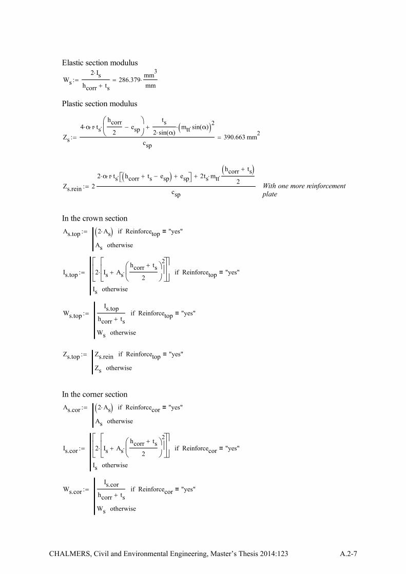
Elastic section modulus
Ws
2 Is
hcorr ts286.379
mm3
mm
Plastic section modulus
Zs
4 α r tshcorr
2esp
ts
2 sin α( )mtt sin α( ) 2
csp390.663 mm
2
Zs.rein 2
2 α r ts hcorr ts esp esp 2ts mtthcorr ts
2
csp With one more reinforcement
plate
In the crown section
As.top 2 As Reinforcetop "yes"=if
As otherwise
Is.top 2 Is As
hcorr ts
2
2
Reinforcetop "yes"=if
Is otherwise
Ws.top
Is.top
hcorr tsReinforcetop "yes"=if
Ws otherwise
Zs.top Zs.rein Reinforcetop "yes"=if
Zs otherwise
In the corner section
As.cor 2 As Reinforcecor "yes"=if
As otherwise
Is.cor 2 Is As
hcorr ts
2
2
Reinforcecor "yes"=if
Is otherwise
Ws.cor
Is.cor
hcorr tsReinforcecor "yes"=if
Ws otherwise
CHALMERS, Civil and Environmental Engineering, Master’s Thesis 2014:123 A.2-7

Zs.cor Zs.rein Reinforcecor "yes"=if
Zs otherwise
Summary of chosen cross-section properties
As 9.08mm
2
mm Is 2.105 10
4
mm4
mm
Ws 286.379mm
3
mm Zs 390.663
mm3
mm
Considering the reinforcement plate in the top section
As.top 18.16mm
2
mm Is.top 1.402 10
5
mm4
mm
Ws.top 953.77mm
3
mm Zs.top 1.335 10
3
mm3
mm
Considering the reinforcement plate in the corner section
As.cor 18.16mm
2
mm Is.cor 1.402 10
5
mm4
mm
Ws.cor 953.77mm
3
mm Zs.cor 1.335 10
3
mm3
mm
2.3. Relative stiffness between the culvert and the surrounding soil
Stiffsoil Esoil.d D3
5.18 1010
J
Stiffsteel Es Is 4.42 106
J
λf
Stiffsoil
Stiffsteel11718.7 The main limitation of stiffness number is:
100 < λf < 100,000
2.4. Reduction of the effective height of soil cover
hc.red hc 0.015 D 565.95 mm
2.5. Dynamic amplification factor
If loads from Swedish bridge code Bro 2004 are applied, a reduction is introducedprovided that the cover depth is high.
A.2-8 CHALMERS, Civil and Environmental Engineering, Master’s Thesis 2014:123

rd 1 hc.red 2mif
1.1 0.05hc.red
m
2m hc.red 6mif
0.8 6m hc.redif
rd 1
For loads from Eurocode, the consideration about reduction factor is not needed.
2.6. Determination of normal forces
Normal force due to the surrounding soil
Nsurr 0.2H
Dρ1 D
2 134.603
kN
m When the backfilling reaches the crown
level
Ncover Sar 0.9hc.red
D 0.5
hc.red
D
H
D
ρcv D2
Due to the soil cover only
Ncover 107.818kN
m
Normal force due to live traffic loads
Since the distributed live load q in the equation below is taken into considerationin the calculation of equivalent line load with the Boussinesq method, so
q 0kN
m
Nt ptrafficD
2
q
hc.red
D0.25if
1.25hc.red
D
ptrafficD
2
q
0.25hc.red
D 0.75if
0.5 ptrafficD
2
q
otherwise
Nt 162.5kN
m
Nt.fatigue ptraffic.fatigueD
2
q
hc.red
D0.25if
1.25hc.red
D
ptraffic.fatigueD
2
q
0.25hc.red
D 0.75if
0.5 ptraffic.fatigueD
2
q
otherwise
Nt.fatigue 57.1kN
m
CHALMERS, Civil and Environmental Engineering, Master’s Thesis 2014:123 A.2-9
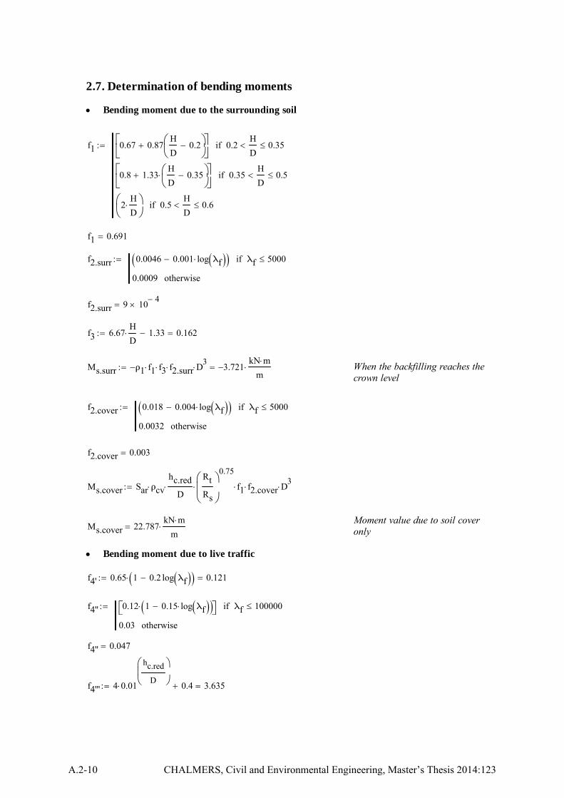
2.7. Determination of bending moments
Bending moment due to the surrounding soil
f1 0.67 0.87H
D0.2
0.2H
D 0.35if
0.8 1.33H
D0.35
0.35H
D 0.5if
2H
D
0.5H
D 0.6if
f1 0.691
f2.surr 0.0046 0.001 log λf λf 5000if
0.0009 otherwise
f2.surr 9 104
f3 6.67H
D 1.33 0.162
Ms.surr ρ1 f1 f3 f2.surr D3
3.721kN m
m When the backfilling reaches the
crown level
f2.cover 0.018 0.004 log λf λf 5000if
0.0032 otherwise
f2.cover 0.003
Ms.cover Sar ρcvhc.red
D
Rt
Rs
0.75
f1 f2.cover D3
Moment value due to soil coveronlyMs.cover 22.787
kN m
m
Bending moment due to live traffic
f4' 0.65 1 0.2 log λf 0.121
f4'' 0.12 1 0.15 log λf λf 100000if
0.03 otherwise
f4'' 0.047
f4''' 4 0.01
hc.red
D
0.4 3.635
A.2-10 CHALMERS, Civil and Environmental Engineering, Master’s Thesis 2014:123

check "OK" f4' f4''' 1if
"ERROR" otherwise
check "OK"
f4.IV
Rt
Rs
0.25
1.831
Moment value due to traffic only
Mt f4' f4'' f4''' f4.IV D ptraffic Sar
Rt
Rs
0.75
f1 f2.cover q D2
75.12kN m
m
Mt.fatigue f4' f4'' f4''' f4.IV D ptraffic.fatigue Sar
Rt
Rs
0.75
f1 f2.cover q D2
26.396kN m
m
3. Design value of normal forces and bending moments
3.1. Normal forces
Regarding normal forces, the loads due to both the soil and the live traffic are unfavorable.
Scenario 1: Backfilling reaches the crown level
The load due to surrounding soil is considered as a live load in this stage.
Nd.SLS.1 max γQ.s Nsurr 134.603kN
m
Scenario 2: Backfilling completed
SLS
Nd.SLS.2 max γG.s Nsurr Ncover max γQ.s Nt
Nd.SLS.2 404.922kN
m
ULS
Nd.ULS.2 max γG.u Nsurr Ncover max γQ.u Nt
Nd.ULS.2 546.644kN
m
3.2. Bending moment
Definition:Negative bending moments at the crown are due to surrounding soil till crown level;Positive bending moments at the crown are due to cover soil and live traffic load.
Thus, for the calculation of each bending moment, there are two possible load
CHALMERS, Civil and Environmental Engineering, Master’s Thesis 2014:123 A.2-11
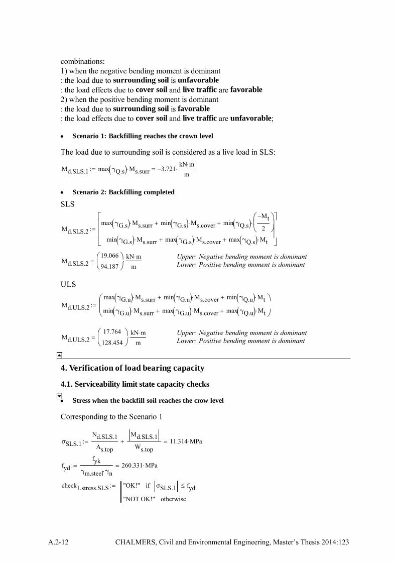
combinations:1) when the negative bending moment is dominant: the load due to surrounding soil is unfavorable: the load effects due to cover soil and live traffic are favorable2) when the positive bending moment is dominant: the load due to surrounding soil is favorable : the load effects due to cover soil and live traffic are unfavorable;
Scenario 1: Backfilling reaches the crown level
The load due to surrounding soil is considered as a live load in SLS:
Md.SLS.1 max γQ.s Ms.surr 3.721kN m
m
Scenario 2: Backfilling completed
SLS
Md.SLS.2max γG.s Ms.surr min γG.s Ms.cover min γQ.s
Mt
2
min γG.s Ms.surr max γG.s Ms.cover max γQ.s Mt
Upper: Negative bending moment is dominantLower: Positive bending moment is dominantMd.SLS.2
19.066
94.187
kN m
m
ULS
Md.ULS.2
max γG.u Ms.surr min γG.u Ms.cover min γQ.u Mt
min γG.u Ms.surr max γG.u Ms.cover max γQ.u Mt
Upper: Negative bending moment is dominantLower: Positive bending moment is dominantMd.ULS.2
17.764
128.454
kN m
m
4. Verification of load bearing capacity
4.1. Serviceability limit state capacity checks
Stress when the backfill soil reaches the crow level
Corresponding to the Scenario 1
σSLS.1
Nd.SLS.1
As.top
Md.SLS.1
Ws.top 11.314 MPa
fyd
fyk
γm.steel γn260.331 MPa
check1.stress.SLS "OK!" σSLS.1 fydif
"NOT OK!" otherwise
A.2-12 CHALMERS, Civil and Environmental Engineering, Master’s Thesis 2014:123
check1.stress.SLS "OK!"
factor1.stress.SLS
σSLS.1
fyd0.043
Stress when the backfilling process is complete
Corresponding to the Scenario 2
σSLS.2
Nd.SLS.2
As.top
Md.SLS.20
Ws.top
Nd.SLS.2
As.top
Md.SLS.21
Ws.top
σSLS.242.287
121.049
MPa Upper: Negative bending moment is dominantLower: Positive bending moment is dominant
σSLS.max max σSLS.2
σSLS.max 121.049 MPa
check2.stress.SLS "OK!" σSLS.max fydif
"NOT OK!" otherwise
check2.stress.SLS "OK!"
factor2.stress.SLS
σSLS.max
fyd0.465
4.2. Ultimate limit state capacity checks
4.2.1. Local buckling
According to Appendix 1 in the Handbook, the chosen corrugated profile must be checkedregarding the risk of local buckling.
Mu Zs
fyk
γM1 123.059
kN m
m Plastic moment capacity
Mucr 1.429 0.156 lnmtt
ts
fyk
227MPa
Mu 120.503 kNm
m
Riskof.local.buckling
Mucr
Mu0.979
check3.local.buckling "No risk of local buckling" Riskof.local.buckling 1if
"Risk of local buckling exists" otherwise
CHALMERS, Civil and Environmental Engineering, Master’s Thesis 2014:123 A.2-13
check3.local.buckling "Risk of local buckling exists"
factor3.local.buckling min 1 Riskof.local.buckling
factor3.local.buckling 0.979 This factor will be used to reduce the plastic momentcapacity if risk of local buckling exists.
4.2.2. Check for the plastic hinge in the crown of the culvert
According to Section 5.3 in Handbook, the check against flexural buckling of the upperpart of the pipe capacity is adapted based on EN 1993-1-1. The section properties of the plates used for the culverts can be assumed in cross-sectionclass 1 or 2. Thus, reduciton due to local buckling can be omitted.
Two conditions to be verified:
Check the maximum loaded section
NEd
χy fyk As
γM1
kyy
My.Ed
fyk Zs
γM1
1.0
When Mz.Ed 0 ΔMz.Ed Mz.Ed 0
The plate is presumed not to deflect alony longitudinal direction (z-axis)
χLT 1.0 χZ 1.0
Design forces and moments
NEd Nd.ULS.2 Corresponding to the ULS inScenario 2
NEd 546.644kN
m
My.Ed max Md.ULS.20Md.ULS.21
The worst load combination casein Scenario 2
My.Ed 128.454kN m
m
Ncr for the crown section According to Appendix 5 inHandbook
Κhc
Rt0.066
ξ min Κ 1 0.256
A.2-14 CHALMERS, Civil and Environmental Engineering, Master’s Thesis 2014:123
ηj 11
1 Κ
2
0.119
μ 1.22 1.95Es Is.top
ηj Esoil.d Rt3
0.25
2
1
ηj
8.968
Ncr.el3ξ
μ
Esoil.d Es Is.top
Rt 728.257
kN
m
Nu fyd As.top 4.728 103
kN
m
ωNcr.el
Nu
Ncr.el
Nu0.5if
1 0.25Nu
Ncr.el
otherwise
ω 0.154
Ncr ω Nu 728.257kN
m
Reduction factor for flexuaral buckling -- χy
The relative slenderness
According to EN 1993-1-1,section 6.3.1λbuk
As.top fyk
Ncr2.803
Imperfection factor αbu
αbu 0.49
ϕ 0.5 1 αbu λbuk 0.2 λbuk2
5.065
χy min 11
ϕ ϕ2
λbuk2
χy 0.108
Evaluation of ineraction factor -- kyy
According to Table A.1 & A.2 in Appendix A in EN 1993-1-1 and recommendation givenin Handbook in Section 5.3
Buckling curve C, EN 1993-1-16.3.1Ncr.y Ncr.el 728.257
kN
m
CHALMERS, Civil and Environmental Engineering, Master’s Thesis 2014:123 A.2-15
Maximum theoretical deflection according to Appendix 3 in Handbook
δmax 0.013ρ1 D
2
Esoil.k
H
D
2.8
λf
0.56 0.2 lnH
D
46.28 mm
Equivalent uniform moment factor, Table A.2
Cmy.0 1π
2Es Is.top δmax
D2
My.Ed1
NEd
Ncr.y 0.771
Cmy Cmy.0 0.771
wy min 1.5Zs.top
Ws.top
wy 1.399
npl
NEd
fyk As.top
γM1
0.096
Cyy 1 wy 1 21.6
wyCmy
2 λbuk 1 λbuk
npl
Cyy max Cyy
Ws.top
Zs.top
0.8
kyy
Cmy
1 χy
NEd
Ncr.y
Cyy
1.05
Check the condition
cond1
NEd
χy fyk As.top
γM1
kyy
My.Ed
Zs.top fyk factor3.local.buckling
γM1
1.215
check4.upper.part.pipe "OK!" cond1 1if
"NOT OK" otherwise
check4.upper.part.pipe "NOT OK"
factor4.upper.part.pipe cond1 1.215
A.2-16 CHALMERS, Civil and Environmental Engineering, Master’s Thesis 2014:123

Check the capacity against the maximum normal force when M.d.u = 0
Condition to be verified: Nd.u
ω fyd As.top
αc
1
ηZs.top
Ws.top1.399
αc max 0.8 η2
ω 0.8
Nd.u Nd.ULS.2
cond2
Nd.u
ω fyd As.top
αc
check5.upper.part.pipe "OK!" cond2 1if
"NOT OK" otherwise
check5.upper.part.pipe "OK!"
factor5.upper.part.pipe cond2 0.795
4.2.3. Check for the plastic hinge in the corner section of the box culvert
Two conditions to be verified:
Check the maximum loaded case
NEd
χy fyk As
γM1
kyy
My.Ed
fyk Zs
γM1
1.0
Design forces and momentsCorresponding to the ULS inScenario 2
NEd.cor Nd.ULS.2
NEd.cor 546.644kN
m
Md.ULS.2.cor
2
3max γG.u Ms.surr min γG.u Ms.cover 1
3min γQ.u Mt
2
3min γG.u Ms.surr max γG.u Ms.cover 1
3max γQ.u Mt
CHALMERS, Civil and Environmental Engineering, Master’s Thesis 2014:123 A.2-17

My.Ed.cor max Md.ULS.2.cor0Md.ULS.2.cor1
My.Ed.cor 51.832kN m
m
Ncr for the corner section According to Appendix 5 inHandbook
Κcor
hc
Rs0.738
ξcor min Κcor 1 0.859
ηj.cor 11
1 Κcor
2
0.669
μcor 1.22 1.95Es Is.cor
ηj.cor Esoil.d Rs3
0.25
2
1
ηj.cor
13.941
Ncr.el.cor
3ξcor
μcor
Esoil.d Es Is.cor
Rs 5.271 10
3
kN
m
Nu.cor fyd As.cor 4.728 103
kN
m
ωcor
Ncr.el.cor
Nu.cor
Ncr.el.cor
Nu.cor0.5if
1 0.25Nu.cor
Ncr.el.cor
otherwise
ωcor 0.776
Ncr.cor ωcor Nu.cor 3.668 103
kN
m
Reduction factor for flexuaral buckling -- χy.cor
According to EN 1993-1-1, section 6.3.1
λbuk
As.cor fyk
Ncr.cor1.249 The relative slenderness
Imperfection factor αbu
αbu 0.49 Buckling curve C, EN 1993-1-1 6.3.1
A.2-18 CHALMERS, Civil and Environmental Engineering, Master’s Thesis 2014:123

ϕ 0.5 1 αbu λbuk 0.2 λbuk2
1.537
χy.cor min 11
ϕ ϕ2
λbuk2
χy.cor 0.411
Evaluation of ineraction factor -- kyy.cor
According to Table A.1 & A.2 in Appendix A in EN 1993-1-1 and recommendation givenin Handbook in Section 5.3
Ncr.y Ncr.el.cor 5.271 103
kN
m
Equivalent uniform moment factor, Table A.2
Cmy.0 1π
2Es Is.cor δmax
D2
My.Ed1
NEd
Ncr.y 0.968
Cmy Cmy.0 0.968
wy min 1.5Zs.cor
Ws.cor
wy 1.399
npl
NEd.cor
fyk As.cor
γM1
0.096
Cyy 1 wy 1 21.6
wyCmy
2 λbuk 1 λbuk
npl 0.961
Cyy max Cyy
Ws.cor
Zs.cor
0.961
kyy.cor
Cmy
1 χy
NEd.cor
Ncr.y
Cyy
1.019
Check the condition
CHALMERS, Civil and Environmental Engineering, Master’s Thesis 2014:123 A.2-19

cond1
NEd.cor
χy.cor fyk As.cor
γM1
kyy.cor
My.Ed.cor
Zs.cor fyk factor3.local.buckling
γM1
0.361
check6.corner.part.pipe "OK!" cond1 1if
"NOT OK" otherwise
check6.corner.part.pipe "OK!"
factor6.corner.part.pipe cond1 0.361
Check the capacity against the maximum normal force when M.d.u = 0
Condition to be verified: Nd.u
ωcor fyd As.cor
αc
1
ηcor
Zs.cor
Ws.cor1.399
αc max 0.8 ηcor2
ωcor
1.519
Nd.u.cor Nd.ULS.2
cond2
Nd.u.cor
ωcor fyd As.cor
αc
check7.corner.part.pipe "OK!" cond2 1if
"NOT OK" otherwise
check7.corner.part.pipe "OK!"
factor7.corner.part.pipe cond2 0.055
4.2.4. Check for capacity of the bolt connection
The ULS checks of bolted connections in this section are according to the Section 5.3 ofHandbook, which is adapted to Eurocode.
Shear capacity
Fv.Rd 0.6Abolt
fub
1.05 γn 130.56 kN Shear resistence per bolt
Fb.Rd
2.5 fuk dbolt ts
1.05 γn142.424 kN Bearing resistence per bolt
A.2-20 CHALMERS, Civil and Environmental Engineering, Master’s Thesis 2014:123

Nd.ULS Nd.ULS.2 546.644kN
m
check8.bolt.shear "OK!" Nd.ULS min nbolt Fv.Rd nbolt Fb.Rd if
"Not OK" otherwise
check8.bolt.shear "OK!"
factor8.bolt.shear
Nd.ULS
min nbolt Fv.Rd nbolt Fb.Rd 0.279
Tension capacity
Figure: Notations used when determining the distance between bolts
Ft.Rd 0.9fub Abolt
1.05 γn 195.84 kN
Md.ULS max Md.ULS.2 128.454kN m
m
check9.bolt.tension "OK!" Md.ULS abolt
nbolt Ft.Rd
2if
"Not OK" otherwise
check9.bolt.tension "OK!"
factor9.bolt.tension
Md.ULS
abolt
nbolt Ft.Rd
2
0.46
Interaction
Fst 2Md.ULS
abolt nbolt 90.143 kN
Ft.Ed Fst
Fsv
Nd.ULS
nbolt36.443 kN
Fv.Ed Fsv
CHALMERS, Civil and Environmental Engineering, Master’s Thesis 2014:123 A.2-21

InteractionFv.Ed
Fv.Rd
Ft.Ed
1.4 Ft.Rd 0.608
check10.bolt.interaction "OK!" Interaction 1if
"Not OK" otherwise
factor10.bolt.interaction Interaction 0.608
4.3. Fatigue checks
4.3.1. Check the fatigue of the plate at the crown seciton
Range values of normal force and bending moment due to LM3
ΔNt.f Nt.fatigue 57.1kN
m
ΔMt.f Mt.fatigue 1.5 39.594kN m
m Equation 4.ab, Section 4.4.5
Handbook
Stresses in the plate material due to fatigue loading
According to section 4.4.5 in the handbook, the minimum moment due to traffic load isassumed to be half of the maxium moment bending in opposite direction.
Stress at top fiber
σtop.c
ΔNt.f
As.top
ΔMt.f
Ws.top 44.658 MPa Compression
σtop.t
ΔNt.f
As.top
ΔMt.f
2
Ws.top 17.612 MPa Tension
Stress at bottom fiber
σbott.t
ΔNt.f
As.top
ΔMt.f
Ws.top 38.369 MPa Tension
σbott.c
ΔNt.f
As.top
ΔMt.f
2
Ws.top 23.901 MPa Compression
The effective stress range at the crown section due to LM3
Δσtop 60% σtop.c σtop.t 44.407 MPa Figure 7.4, Section 7.2.1,EN 1993-1-9
Δσbott 60% σbott.c σbott.t 52.71 MPa
A.2-22 CHALMERS, Civil and Environmental Engineering, Master’s Thesis 2014:123
Δσp max Δσtop Δσbott 52.71 MPa
The damage equivalent stress range related to 2 million cycles
ΔσE.2.p =:λ ϕ 2⋅Δσp Section 9.4.1, EN 1993-2
Damage equivalent impact factor
ϕ2 1
Damage equivalence factor
λ λ1 λ2 λ3 λ4 λ1 and λ λmax
λ1--factor for damage effect of traffic, according to Figure 9.5 EN 1993-2
λ1 2.25 D 10mif
2.25 0.7D 10m( )
70m
otherwise
λ1 2.227
λ2--factor for traffic volume according to Table 9.1 EN 1993-2
Q0 480kN N0 0.5 106
Recommended in Section 9.5.2
Average gross weight of lorries in the slow lane
Qm1 300kN
Number of heavy vehicles per year per slow lane
Category 2, table 4.5 (n), EN 1991-2 , whichcorresponding to 1500<ADT heavy traffic < 6000 inB3.2.1.3, TRAFIKVERKET TRVK BRO 11,Publ nr2011:085
Nobs 0.5 106
λ2
Qm1
Q0
Nobs
N0
1
5
λ2 0.625
λ3--factor for design life for the bridge according to Table 9.2 EN 1993-2
tLd 80Assumption of design life span
CHALMERS, Civil and Environmental Engineering, Master’s Thesis 2014:123 A.2-23

λ3
tLd
100
1
5
0.956
λ4--factor for traffic in the other lanes
λ4 1 According to the guidance from National Annex,VVFS 2009, Page 34
λmax 2.5 D 10mif
2.5 0.5D 10m
15m
otherwise
λmax 2.424
So,
λ min λ1 λ2 λ3 λ4 λmax 1.331
ΔσE.2.p λ ϕ2 Δσp 70.173 MPa
Fatigue verification
The section category for the plate
Δσc.p 125MPa Detail 5 in Table 8.1, EN 1993-1-9
check11.fatigue.plate "OK!"γFf ΔσE.2.p
Δσc.p
γMf
1 ΔσE.2.p 1.5 fykif
"Not OK, Plate Fatigue" otherwise
check11.fatigue.plate "OK!"
factor11.fatigue.plate
γFf ΔσE.2.p
Δσc.p
γMf
0.758
4.3.2 Check the fatigue of bolted connections
A.2-24 CHALMERS, Civil and Environmental Engineering, Master’s Thesis 2014:123

Figure When the joints are situated at positions with greater depth of cover than at thecrown, the designing moment due to fatigue can be reduced
Assume the position of bolted connection at depth hf
hf
hc
0.85
Fatigue of bolts
Shear force on each bolt in the connection due to normal force
ΔFd.v
ΔNt.f
nbolt3.807 kN
Shear stress
ΔτE.2.b λ ϕ2ΔFd.v
Abolt 16.131 MPa
Δτc 100MPa Detail 15, Table 8.1, EN 1993-1-9
Tensile force on each bolt in the connection due to bending moment
ΔFd.t
2ΔMt.f
abolt
hc
hf
nbolt23.618 kN
Tensile stress
ΔσE.2.b λ ϕ2ΔFd.t
Abolt 100.084 MPa
Δσc 50MPa Detail 14, Table 8.1, EN 1993-1-9
Fatigue verification According to section 8 EN 1993-1-9
Shear stress
CHALMERS, Civil and Environmental Engineering, Master’s Thesis 2014:123 A.2-25
check12.fatigue.shear "OK!"γFf ΔτE.2.b
Δτc
γMf
1 ΔτE.2.b 1.5fuk
3if
"Not OK, Shear stress fatigue in bolts" otherwise
check12.fatigue.shear "OK!"
factor12.fatigue.shear
γFf ΔτE.2.b
Δτc
γMf
0.218
Tensile stress
check13.fatigue.tension "OK!"γFf ΔσE.2.b
Δσc
γMf
1 ΔσE.2.b 1.5 fukif
"Not OK, Shear stress fatigue in bolts" otherwise
check13.fatigue.tension "Not OK, Shear stress fatigue in bolts"
factor13.fatigue.tension
γFf ΔσE.2.b
Δσc
γMf
2.702
Interaction of shear and tension
interactionfatigue
γFf ΔσE.2.b
Δσc
γMf
3γFf ΔτE.2.b
Δτc
γMf
5
19.733
check14.fatigue.interaction "OK!" interactionfatigue 1if
"Not OK, Fatigue in bolts" otherwise
factor14.fatigue.interaction interactionfatigue 19.733
4.4. Structural stiffness check
This check ensures that the culvert structure has adequate rigidity during installation andhandling processs.
A.2-26 CHALMERS, Civil and Environmental Engineering, Master’s Thesis 2014:123
stiffnessD
2
Es Is0.034
m
kN
ηm 0.2m
kN According to Section 5.2 Handbook,
0.2 m/kN--for arched and low-rise sections;0.13 m/kN--for circular sections
check15.stiff "OK!" stiffness ηmif
"Not OK" otherwise
check15.stiff "OK!"
stiffness 0.034m
kN
5. Summary
5.1. Input data
Geometry
Culvert profile profile "G: Box Culvert"
Span D 12.27 m
Soil cover hc 750 mm
Corrugated steel plates
Type of plate typesteel 2 Type 1: 200*55; Type 2: SuperCor
Thickness of plate ts 7 mm Reinforcetop "yes" Reinforcecor "yes"
Bolts
Diameter of bolts dbolt 20 mm
Bolt class 8.8 fub 800 MPa
Number of bolts per meter nbolt 15 m1
Loads
Traffic load ptraffic 162.5kN
m
Traffic load-fatigue ptraffic.fatigue 57.1kN
m
5.2. Checks
Serviceability limit state capacity checks
CHALMERS, Civil and Environmental Engineering, Master’s Thesis 2014:123 A.2-27
check1.stress.SLS "OK!" Backfill till the crown levelfactor1.stress.SLS 0.043
check2.stress.SLS "OK!" After soil cover completedfactor2.stress.SLS 0.465
Ultimate limit state capacity checks
Check for the plastic hinge in the upper part of the culvert
check4.upper.part.pipe "NOT OK" Considering normal force and bending moment
factor4.upper.part.pipe 1.215
check5.upper.part.pipe "OK!" Considering normal force only
factor5.upper.part.pipe 0.795
Check for capacity in the corner of the pipe
check6.corner.part.pipe "OK!" Considering normal force and bending moment
factor6.corner.part.pipe 0.361
check7.corner.part.pipe "OK!" Considering normal force only
factor7.corner.part.pipe 0.055
Check for capacity of bolts
check8.bolt.shear "OK!" Considering shear stress only
factor8.bolt.shear 0.279
check9.bolt.tension "OK!" Considering tensile stress only
factor9.bolt.tension 0.46
check10.bolt.interaction "OK!" Considering interaction of shear and tension
factor10.bolt.interaction 0.608
fatigue checks
Check the fatigue of the plate at the crown seciton
check11.fatigue.plate "OK!"
factor11.fatigue.plate 0.758
Check the fatigue of bolted connections
A.2-28 CHALMERS, Civil and Environmental Engineering, Master’s Thesis 2014:123
check12.fatigue.shear "OK!"
factor12.fatigue.shear 0.218
check13.fatigue.tension "Not OK, Shear stress fatigue in bolts"
factor13.fatigue.tension 2.702
check14.fatigue.interaction "Not OK, Fatigue in bolts"
factor14.fatigue.interaction 19.733
Other checks
Local buckling
check3.local.buckling "Risk of local buckling exists"
factor3.local.buckling 0.979
Structural stiffness check
check15.stiff "OK!"
CHALMERS, Civil and Environmental Engineering, Master’s Thesis 2014:123 A.2-29
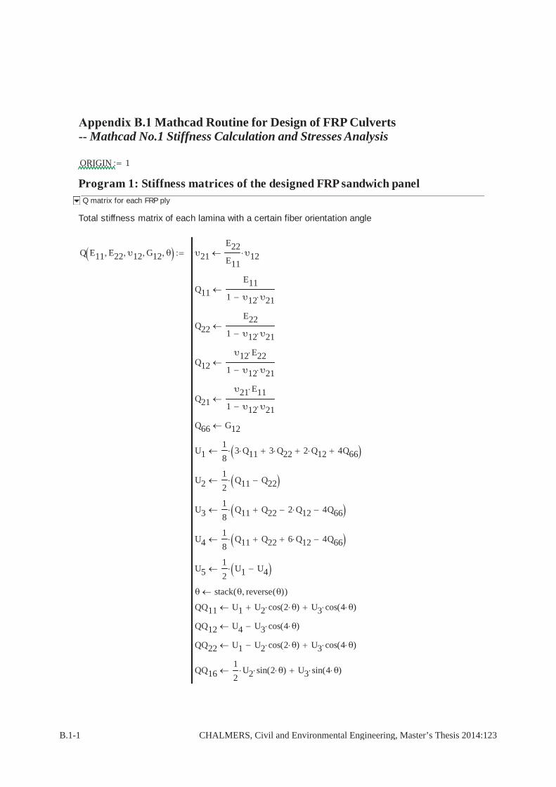
Mathcad Routine for Design of FRP Culverts-- Mathcad No.1 Stiffness Calculation and Stresses Analysis
ORIGIN 1
Program 1: Stiffness matrices of the designed FRP sandwich panelQ matrix for each FRP ply
Total stiffness matrix of each lamina with a certain fiber orientation angle
Q E11 E22 υ12 G12 θ υ21
E22
E11υ12
Q11
E11
1 υ12 υ21
Q22
E22
1 υ12 υ21
Q12
υ12 E22
1 υ12 υ21
Q21
υ21 E11
1 υ12 υ21
Q66 G12
U11
83 Q11 3 Q22 2 Q12 4Q66
U21
2Q11 Q22
U31
8Q11 Q22 2 Q12 4Q66
U41
8Q11 Q22 6 Q12 4Q66
U51
2U1 U4
θ stack θ reverse θ( )( )
QQ11 U1 U2 cos 2 θ( ) U3 cos 4 θ( )
QQ12 U4 U3 cos 4 θ( )
QQ22 U1 U2 cos 2 θ( ) U3 cos 4 θ( )
QQ161
2U2 sin 2 θ( ) U3 sin 4 θ( )
B.1-1 CHALMERS, Civil and Environmental Engineering, Master’s Thesis 2014:123

QQ261
2U2 sin 2 θ( ) U3 sin 4 θ( )
QQ66 U5 U3 cos 4 θ( )
QQ11
QQ12
QQ16
QQ12
QQ22
QQ26
QQ16
QQ26
QQ66
Q matrix for each FRP ply
Coordinates of each FRP ply
hi refers to the distance from the midplane to the top of the ith lamina.
h t no d( )
hi
t no 2 d( )
2i 1( ) t
i 1 no 1( )for
hi
t no 2 d( )
2d i 2( ) t
i no 2( ) 2no 2( )for
hreturn
Coordinates of each FRP ply
Matrices A B D for the FRP Sandwich
Extensional stiffness matrix for the FRP sandwich (unite: N/m)
A E11 E22 υ12 G12 θ t no d
hai
h t no d( )i 1( )
h t no d( )i
i 1 nofor
hai
h t no d( )i 2( )
h t no d( )i 1( )
i no 1( ) 2 no( )for
Ai j
Q E11 E22 υ12 G12 θ i j ha
j 1 3for
i 1 3for
A
Coupling stiffness matrix for the FRP sandwich (unit: N)
CHALMERS, Civil and Environmental Engineering, Master’s Thesis 2014:123 B.1-2
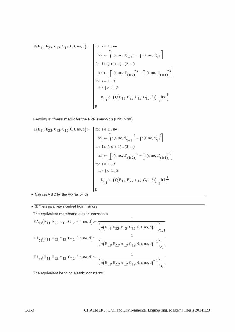
B E11 E22 υ12 G12 θ t no d
hbi
h t no d( )i 1
2h t no d( )
i2
i 1 nofor
hbi
h t no d( )i 2( )
2h t no d( )
i 1( )2
i no 1( ) 2 no( )for
Bi j
Q E11 E22 υ12 G12 θi j
hb1
2
j 1 3for
i 1 3for
B
Bending stiffness matrix for the FRP sandwich (unit: N*m)
D E11 E22 υ12 G12 θ t no d
hdi
h t no d( )i 1
3h t no d( )
i3
i 1 nofor
hdi
h t no d( )i 2( )
3h t no d( )
i 1( )3
i no 1( ) 2 no( )for
Di j
Q E11 E22 υ12 G12 θi j
hd1
3
j 1 3for
i 1 3for
DMatrices A B D for the FRP Sandwich
Stiffness parameters derived from matrices
The equivalent membrane elastic constants
EAxx E11 E22 υ12 G12 θ t no d1
A E11 E22 υ12 G12 θ t no d1
1 1
EAyy E11 E22 υ12 G12 θ t no d1
A E11 E22 υ12 G12 θ t no d1
2 2
EAxy E11 E22 υ12 G12 θ t no d1
A E11 E22 υ12 G12 θ t no d1
3 3
The equivalent bending elastic constants
B.1-3 CHALMERS, Civil and Environmental Engineering, Master’s Thesis 2014:123

EIxx E11 E22 υ12 G12 θ t no d1
D E11 E22 υ12 G12 θ t no d1
1 1
EIyy E11 E22 υ12 G12 θ t no d1
D E11 E22 υ12 G12 θ t no d1
2 2
EIxy E11 E22 υ12 G12 θ t no d1
D E11 E22 υ12 G12 θ t no d1
3 3Stiffness parameters derived from matrices
Program 2: Stresses analysis of FRP sandwich panel in each FRP ply
Midplane strains and curvatures due to sectional forces
D1 E11 E22 υ12 G12 θ t no d D D E11 E22 υ12 G12 θ t no d
Ainv A E11 E22 υ12 G12 θ t no d1
B B E11 E22 υ12 G12 θ t no d
D1 D B Ainv B( )1
A1 E11 E22 υ12 G12 θ t no d D1 D1 E11 E22 υ12 G12 θ t no d
Ainv A E11 E22 υ12 G12 θ t no d1
B B E11 E22 υ12 G12 θ t no d
A1 Ainv Ainv B D1 B Ainv
B1 E11 E22 υ12 G12 θ t no d D1 D1 E11 E22 υ12 G12 θ t no d
Ainv A E11 E22 υ12 G12 θ t no d1
B B E11 E22 υ12 G12 θ t no d
B1 Ainv B D1
C1 E11 E22 υ12 G12 θ t no d D1 D1 E11 E22 υ12 G12 θ t no d
Ainv A E11 E22 υ12 G12 θ t no d1
B B E11 E22 υ12 G12 θ t no d
C1 D1 B Ainv
For a symmetric laminate, [B]=[0], and therefore, [A1]=[A-1], [B1]=[C1]=[0], and [D1]=[D-1]
CHALMERS, Civil and Environmental Engineering, Master’s Thesis 2014:123 B.1-4
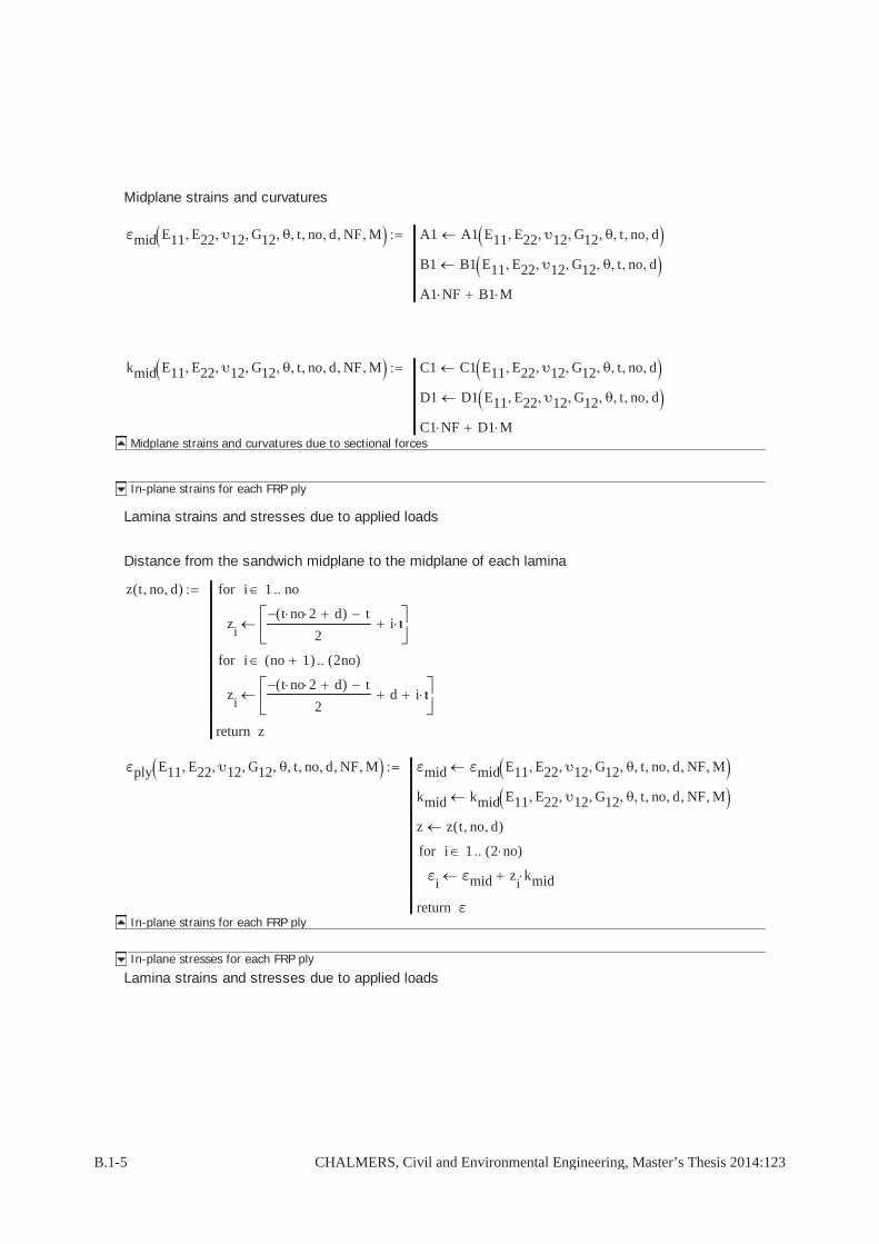
Midplane strains and curvatures
εmid E11 E22 υ12 G12 θ t no d NF M A1 A1 E11 E22 υ12 G12 θ t no d
B1 B1 E11 E22 υ12 G12 θ t no d
A1 NF B1 M
kmid E11 E22 υ12 G12 θ t no d NF M C1 C1 E11 E22 υ12 G12 θ t no d
D1 D1 E11 E22 υ12 G12 θ t no d
C1 NF D1 MMidplane strains and curvatures due to sectional forces
In-plane strains for each FRP ply
Lamina strains and stresses due to applied loads
Distance from the sandwich midplane to the midplane of each lamina
z t no d( )
zi
t no 2 d( ) t
2i t
i 1 nofor
zi
t no 2 d( ) t
2d i t
i no 1( ) 2no( )for
zreturn
εply E11 E22 υ12 G12 θ t no d NF M εmid εmid E11 E22 υ12 G12 θ t no d NF M
kmid kmid E11 E22 υ12 G12 θ t no d NF M
z z t no d( )
εi
εmid zi
kmid
i 1 2 no( )for
εreturnIn-plane strains for each FRP ply
In-plane stresses for each FRP ply
Lamina strains and stresses due to applied loads
B.1-5 CHALMERS, Civil and Environmental Engineering, Master’s Thesis 2014:123

Qply E11 E22 υ12 G12 θ no Q Q E11 E22 υ12 G12 θ
QQi
0
0
0
0
0
0
0
0
0
QQi x y
Qx y i
y 1 3for
x 1 3for
i 1 2 no( )for
QQreturn
stress E11 E22 υ12 G12 θ t no d NF M ε εply E11 E22 υ12 G12 θ t no d NF M
Q Qply E11 E22 υ12 G12 θ no
stressi
Qiε
i
i 1 2 no( )for
stressreturn
In-plane stresses for each FRP ply
Design Process
Step 1: Choose the materials for the FRP sandwich panel
Face and Core
Face material Fiber: E-glass Matrix: Epoxy Fiber/Matrix: 45%
Ek.11 38.6GPa Ek.22 8.27GPa Gk.12 4.14GPa
υ12 0.26
Strength
σk.11.c 610MPa σk.22.c 118MPa τk.12 72MPa
σk.11.t 1062MPa σk.22.t 31MPa
Paritial factor for FRP laminate
--according to Eurocomp Design Code and Handbook, Section 2.3.3.2
γM1 1.5 Derivation of properties
CHALMERS, Civil and Environmental Engineering, Master’s Thesis 2014:123 B.1-6

γM2 1.2 Method of manufacture: Resin transfer moulding
γM3 2.5 1.0 for long-term loading in ULS;2.5 for short-term loading in SLS
γM γM1 γM2 γM3 4.5
Design value
E11
Ek.11
γME22
Ek.22
γMG12
Gk.12
γM
σd.11.c
σk.11.c
γMσd.22.c
σk.22.c
γMτd.12
τk.12
γM
σd.11.t
σk.11.t
γMσd.22.t
σk.22.t
γM
Core Material Divinycell H 80 from DIAB
Face and Core
Step 2: Assume a geometry of the FRP sandwich panel and obtain the bending stiffness
Design the thickness of face and core
Thicknesss of face tface 9mm
t 1mm Thickness of each ply
notface
t9 Number of plies for one laminate face
Fiber orientation for each ply (0 degree in the preliminary design)
θ stack 0deg 0deg 0deg 0deg 0deg 0deg 0deg 0deg 0deg( )
CheckInput "OK" no rows θ( )=if
"Error" otherwise
CheckInput "OK"
Initial bending stiffness
Thickness of core d 150mm
EIxx E11 E22 υ12 G12 θ t no d 0.977 106 N m
2
m
Bending stiffness in the top
B.1-7 CHALMERS, Civil and Environmental Engineering, Master’s Thesis 2014:123
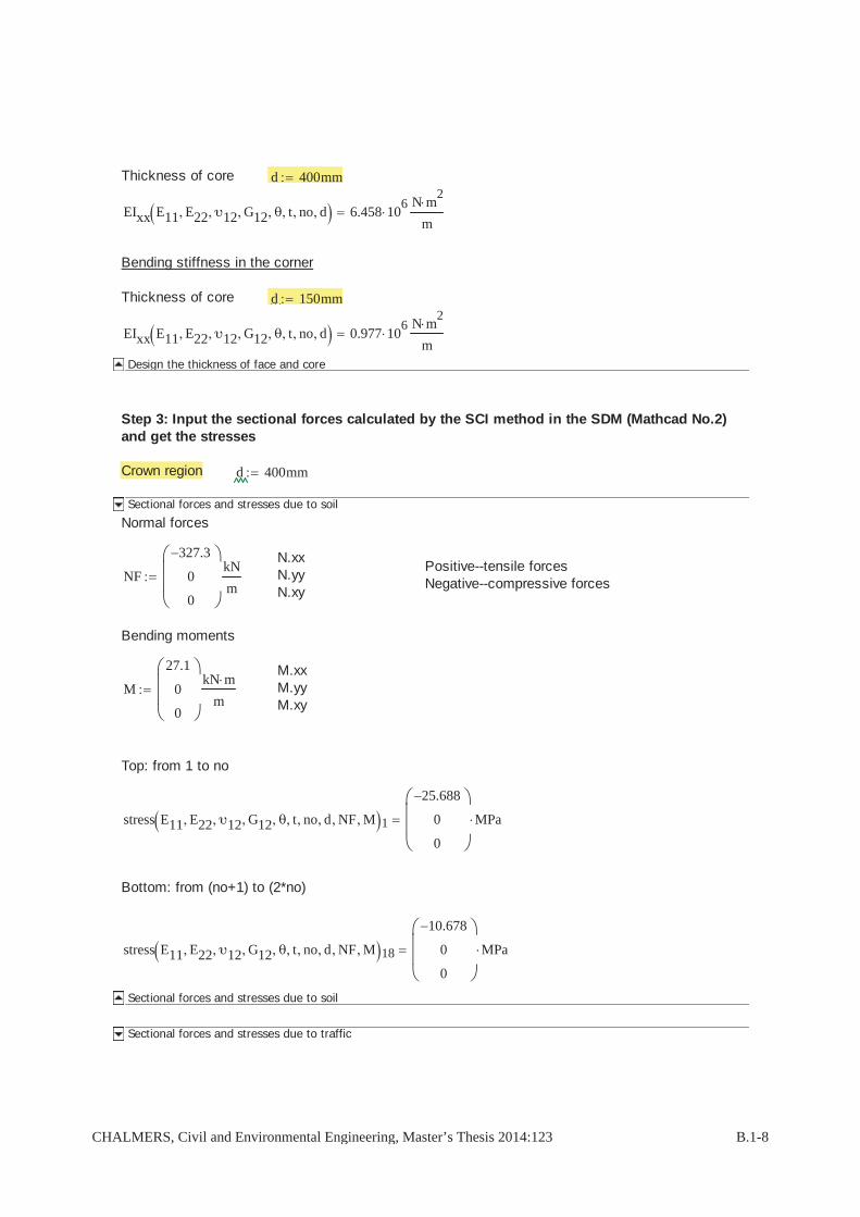
Thickness of core d 400mm
EIxx E11 E22 υ12 G12 θ t no d 6.458 106 N m
2
m
Bending stiffness in the corner
Thickness of core d 150mm
EIxx E11 E22 υ12 G12 θ t no d 0.977 106 N m
2
mDesign the thickness of face and core
Step 3: Input the sectional forces calculated by the SCI method in the SDM (Mathcad No.2)and get the stresses
Crown region d 400mm
Sectional forces and stresses due to soil
Normal forces
N.xx N.yyN.xy
Positive--tensile forcesNegative--compressive forcesNF
327.3
0
0
kN
m
Bending moments
M.xx M.yyM.xy
M
27.1
0
0
kN m
m
Top: from 1 to no
stress E11 E22 υ12 G12 θ t no d NF M 1
25.688
0
0
MPa
Bottom: from (no+1) to (2*no)
stress E11 E22 υ12 G12 θ t no d NF M 18
10.678
0
0
MPa
Sectional forces and stresses due to soil
Sectional forces and stresses due to traffic
CHALMERS, Civil and Environmental Engineering, Master’s Thesis 2014:123 B.1-8

Normal forces
N.xx N.yyN.xy
Positive value for tensile forces;Negative value for compressive forcesNF
219.4
0
0
kN
m
Bending moments
M.xx M.yyM.xy
M
91.3
0
0
kN m
m
Top: from 1 to no
stress E11 E22 υ12 G12 θ t no d NF M 1
37.473
0
0
MPa
Bottom: from (no+1) to (2*no)
stress E11 E22 υ12 G12 θ t no d NF M 18
13.095
0
0
MPa
Sectional forces and stresses due to traffic
Corner region d 150mm
Sectional forces and stresses due to soil
Normal forces
N.xx N.yyN.xy
Positive--tensile forcesNegative--compressive forcesNF
219.4
0
0
kN
m
Bending moments
M.xx M.yyM.xy
M
11.8
0
0
kN m
m
Top: from 1 to no
B.1-9 CHALMERS, Civil and Environmental Engineering, Master’s Thesis 2014:123

stress E11 E22 υ12 G12 θ t no d NF M 1
20.841
0
0
MPa
Bottom: from (no+1) to (2*no)
stress E11 E22 υ12 G12 θ t no d NF M 18
3.537
0
0
MPa
Sectional forces and stresses due to soil
Sectional forces and stresses due to traffic
Normal forces
N.xx N.yyN.xy
Positive value for tensile forces;Negative value for compressive forcesNF
219.4
0
0
kN
m
Bending moments
M.xx M.yyM.xy
M
30.4
0
0
kN m
m
Top: from 1 to no
stress E11 E22 υ12 G12 θ t no d NF M 1
34.478
0
0
MPa
Bottom: from (no+1) to (2*no)
stress E11 E22 υ12 G12 θ t no d NF M 18
10.1
0
0
MPa
Sectional forces and stresses due to traffic
CHALMERS, Civil and Environmental Engineering, Master’s Thesis 2014:123 B.1-10
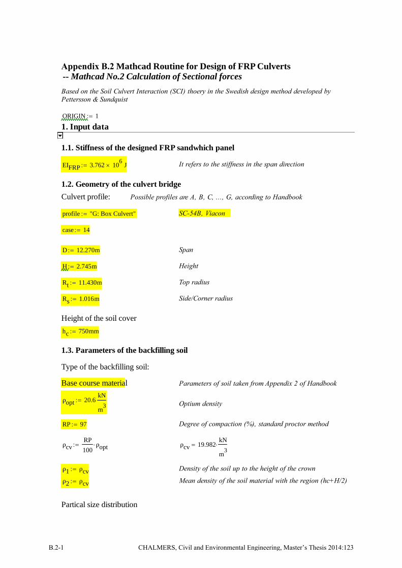
Appendix B.2 Mathcad Routine for Design of FRP Culverts -- Mathcad No.2 Calculation of Sectional forces
Based on the Soil Culvert Interaction (SCI) thoery in the Swedish design method developed byPettersson & Sundquist
ORIGIN 1
1. Input data
1.1. Stiffness of the designed FRP sandwhich panel
It refers to the stiffness in the span direction EIFRP 3.762 106
J
1.2. Geometry of the culvert bridge
Culvert profile: Possible profiles are A, B, C, ..., G, according to Handbook
profile "G: Box Culvert" SC-54B, Viacon
case 14
D 12.270m Span
H 2.745m Height
Rt 11.430m Top radius
Rs 1.016m Side/Corner radius
Height of the soil cover
hc 750mm
1.3. Parameters of the backfilling soil
Type of the backfilling soil:
Base course material Parameters of soil taken from Appendix 2 of Handbook
ρopt 20.6kN
m3
Optium density
RP 97 Degree of compaction (%), standard proctor method
ρcvRP
100ρopt ρcv 19.982
kN
m3
ρ1 ρcv Density of the soil up to the height of the crown
ρ2 ρcv Mean density of the soil material with the region (hc+H/2)
Partical size distribution
B.2-1 CHALMERS, Civil and Environmental Engineering, Master’s Thesis 2014:123
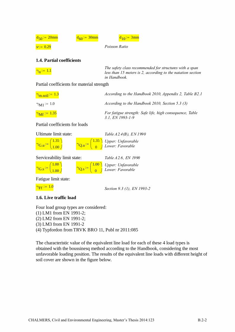
d50 20mm d60 30mm d10 3mm
ν 0.29 Poisson Ratio
1.4. Partial coefficients
The safety class recommended for structures with a spanless than 15 meters is 2, according to the natation sectionin Handbook.
γn 1.1
Partial coefficients for material strength
γm.soil 1.3 According to the Handbook 2010, Appendix 2, Table B2.1
γM1 1.0 According to the Handbook 2010, Section 5.3 (3)
γMf 1.35 For fatigue strength: Safe life, high consequence, Table3.1, EN 1993-1-9
Partial coefficients for loads
Ultimate limit state: Table A2.4(B), EN 1990
Upper: UnfavorableLower: FavorableγG.u
1.35
1.00
γQ.u1.35
0
Serviceability limit state: Table A2.6, EN 1990
Upper: UnfavorableLower: FavorableγG.s
1.00
1.00
γQ.s1.00
0
Fatigue limit state:
γFf 1.0 Section 9.3 (1), EN 1993-2
1.6. Live traffic load
Four load group types are considered: (1) LM1 from EN 1991-2;(2) LM2 from EN 1991-2;(3) LM3 from EN 1991-2(4) Typfordon from TRVK BRO 11, Publ nr 2011:085
The characteristic value of the equivalent line load for each of these 4 load types isobtained with the boussinesq method according to the Handbook, considering the mostunfavorable loading position. The results of the equivalent line loads with different height ofsoil cover are shown in the figure below.
CHALMERS, Civil and Environmental Engineering, Master’s Thesis 2014:123 B.2-2

Figure* The equivalent line load on the culvert crown section at different depth hc
*Note: The Calculation and results of the equivalent line load are provided by the supervisorfrom the consultant company WSP in Gothenburg
The equivalent traffic line load for SLS and ULS
ptraffic 213.7kN
m
hc 0.5m=if
162.5kN
m
hc 0.75m=if
129.2kN
m
hc 1m=if
125.3kN
m
hc 3m=if
"Error" otherwise
ptraffic 162.5kN
m
The equivalent traffic line load due to LM3 for fatigue
B.2-3 CHALMERS, Civil and Environmental Engineering, Master’s Thesis 2014:123

ptraffic.fatigue 72.1kN
m
hc 0.5m=if
57.1kN
m
hc 0.75m=if
49.0kN
m
hc 1m=if
42.6kN
m
hc 3m=if
"Error" otherwise
ptraffic.fatigue 57.1kN
m
2. Calculation
2.1. Soil tangent modulus
Determination of relevant factors
ρs 26kN
m3
True density of the soil material, Appendix 2, Handbook
e1
ρs
ρ11 0.301 Void ratio
Cu
d60
d1010 Uniformity coefficient
m1 282 Cu0.77
e12.83
1.43 103
Modulus ratio
β 0.29 logd50
0.01mm
0.065 log Cu 0.892 Stress exponent
ϕk 26deg 10degRP 75( )
25 0.4deg Cu 1.6deg log
d50
1mm
ϕk 40.882 deg Characteristic angle of internal friction of the backfillmaterial
ϕk.d atantan ϕk
γn γm.soil
31.189 deg Design value of friction angle
Arching effect
Sv1
0.8 tan ϕk.d
1 tan ϕk.d 2 0.45 tan ϕk.d
20.233
κ 2 Sv1hc
D 0.028
CHALMERS, Civil and Environmental Engineering, Master’s Thesis 2014:123 B.2-4

Sar1 e
κ
κ0.986
Tangent modulus of soil material
kv
sin ϕk 3 2 sin ϕk
2 sin ϕk 0.823
Esoil.k 0.42 m1 100 kPa kv
1 sin ϕk ρ2 Sar hcH
2
100kPa
1 β
Esoil.k 40.099 MPa Characteristic value of thetangent modulus
Esoil.d
Esoil.k
γn γm.soil28.041 MPa Design value of the tangent
modulus
2.3. Relative stiffness between the culvert and the surrounding soil
Esoil.d D3
5.18 1010
J
The main limitation of stiffness number is:100 < λf < 100,000 λf
Esoil.d D3
EIFRP13769.2
2.4. Reduction of the effective height of soil cover
hc.red hc 0.015 D 565.95 mm
2.5. Dynamic amplification factor
If loads from Swedish bridge code Bro 2004 are applied, a reduction is introducedprovided that the cover depth is high.
rd 1 hc.red 2mif
1.1 0.05hc.red
m
2m hc.red 6mif
0.8 6m hc.redif
rd 1
For loads from Eurocode, the consideration about reduction factor is not needed.
2.6. Determination of normal forces
Normal force due to the surrounding soil
B.2-5 CHALMERS, Civil and Environmental Engineering, Master’s Thesis 2014:123

Nsurr 0.2H
Dρ1 D
2 134.603
kN
m When the backfilling reaches the crown
level
Ncover Sar 0.9hc.red
D 0.5
hc.red
D
H
D
ρcv D2
Due to the soil cover only
Ncover 107.818kN
m
Normal force due to live traffic loads
Since the distributed live load q in the equation below is taken into considerationin the calculation of equivalent line load with the Boussinesq method, so
q 0kN
m
Nt ptrafficD
2
q
hc.red
D0.25if
1.25hc.red
D
ptrafficD
2
q
0.25hc.red
D 0.75if
0.5 ptrafficD
2
q
otherwise
Nt 162.5kN
m
Nt.fatigue ptraffic.fatigueD
2
q
hc.red
D0.25if
1.25hc.red
D
ptraffic.fatigueD
2
q
0.25hc.red
D 0.75if
0.5 ptraffic.fatigueD
2
q
otherwise
Nt.fatigue 57.1kN
m
2.7. Determination of bending moments
Bending moment due to the surrounding soil
f1 0.67 0.87H
D0.2
0.2H
D 0.35if
0.8 1.33H
D0.35
0.35H
D 0.5if
2H
D
0.5H
D 0.6if
f1 0.691
CHALMERS, Civil and Environmental Engineering, Master’s Thesis 2014:123 B.2-6

f2.surr 0.0046 0.001 log λf λf 5000if
0.0009 otherwise
f2.surr 9 104
f3 6.67H
D 1.33 0.162
Ms.surr ρ1 f1 f3 f2.surr D3
3.721kN m
m When the backfilling reaches the
crown level
f2.cover 0.018 0.004 log λf λf 5000if
0.0032 otherwise
f2.cover 0.003
Ms.cover Sar ρcvhc.red
D
Rt
Rs
0.75
f1 f2.cover D3
Moment value due to soil coveronlyMs.cover 22.787
kN m
m
Bending moment due to live traffic
f4' 0.65 1 0.2 log λf 0.112
f4'' 0.12 1 0.15 log λf λf 100000if
0.03 otherwise
f4'' 0.045
f4''' 4 0.01
hc.red
D
0.4 3.635
check "OK" f4' f4''' 1if
"ERROR" otherwise
check "OK"
f4.IV
Rt
Rs
0.25
1.831
Moment value due to traffic only
Mt f4' f4'' f4''' f4.IV D ptraffic Sar
Rt
Rs
0.75
f1 f2.cover q D2
67.598kN m
m
B.2-7 CHALMERS, Civil and Environmental Engineering, Master’s Thesis 2014:123
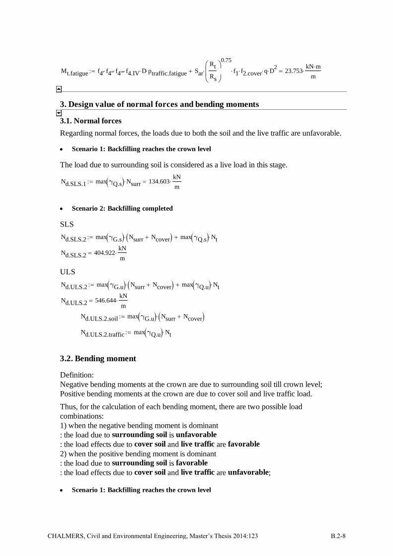
Mt.fatigue f4' f4'' f4''' f4.IV D ptraffic.fatigue Sar
Rt
Rs
0.75
f1 f2.cover q D2
23.753kN m
m
3. Design value of normal forces and bending moments
3.1. Normal forces
Regarding normal forces, the loads due to both the soil and the live traffic are unfavorable.
Scenario 1: Backfilling reaches the crown level
The load due to surrounding soil is considered as a live load in this stage.
Nd.SLS.1 max γQ.s Nsurr 134.603kN
m
Scenario 2: Backfilling completed
SLS
Nd.SLS.2 max γG.s Nsurr Ncover max γQ.s Nt
Nd.SLS.2 404.922kN
m
ULS
Nd.ULS.2 max γG.u Nsurr Ncover max γQ.u Nt
Nd.ULS.2 546.644kN
m
Nd.ULS.2.soil max γG.u Nsurr Ncover
Nd.ULS.2.traffic max γQ.u Nt
3.2. Bending moment
Definition:Negative bending moments at the crown are due to surrounding soil till crown level;Positive bending moments at the crown are due to cover soil and live traffic load.
Thus, for the calculation of each bending moment, there are two possible loadcombinations:1) when the negative bending moment is dominant: the load due to surrounding soil is unfavorable: the load effects due to cover soil and live traffic are favorable2) when the positive bending moment is dominant: the load due to surrounding soil is favorable : the load effects due to cover soil and live traffic are unfavorable;
Scenario 1: Backfilling reaches the crown level
CHALMERS, Civil and Environmental Engineering, Master’s Thesis 2014:123 B.2-8

The load due to surrounding soil is considered as a live load in SLS:
Md.SLS.1 max γQ.s Ms.surr 3.721kN m
m
Scenario 2: Backfilling completed
SLS
Md.SLS.2max γG.s Ms.surr min γG.s Ms.cover min γQ.s
Mt
2
min γG.s Ms.surr max γG.s Ms.cover max γQ.s Mt
Upper: Negative bending moment is dominantLower: Positive bending moment is dominantMd.SLS.2
19.066
86.664
kN m
m
ULS
Md.ULS.2
max γG.u Ms.surr min γG.u Ms.cover min γQ.u Mt
min γG.u Ms.surr max γG.u Ms.cover max γQ.u Mt
Upper: Negative bending moment is dominantLower: Positive bending moment is dominantMd.ULS.2
17.764
118.299
kN m
m
Md.ULS.2.soil
max γG.u Ms.surr min γG.u Ms.cover
min γG.u Ms.surr max γG.u Ms.cover
Md.ULS.2.traffic
min γQ.u Mt
max γQ.u Mt
Md.ULS.2.cor
2
3max γG.u Ms.surr min γG.u Ms.cover 1
3min γQ.u Mt
2
3min γG.u Ms.surr max γG.u Ms.cover 1
3max γQ.u Mt
Md.ULS.2.cor11.843
48.447
kN m
m Upper: Negative bending moment is dominant
Lower: Positive bending moment is dominant
Md.ULS.2.cor.soil
2
3max γG.u Ms.surr min γG.u Ms.cover
2
3min γG.u Ms.surr max γG.u Ms.cover
Md.ULS.2.cor.traffic
1
3min γQ.u Mt
1
3max γQ.u Mt
B.2-9 CHALMERS, Civil and Environmental Engineering, Master’s Thesis 2014:123

4. Summary
Geometry
Culvert profile profile "G: Box Culvert" case 14
Span D 12.27 m
Soil cover hc 750 mm
Loads ptraffic 162.5
kN
mTraffic load
Stiffness
EIFRP 3.762 106
N m
Sectional forces
Nd.SLS.1 134.603kN
m
Nd.SLS.2 404.922kN
m
Nd.ULS.2 546.644kN
m
Nd.ULS.2.soil 327.269kN
m
Nd.ULS.2.traffic 219.375kN
m
Md.SLS.1 3.721 kN
Md.SLS.219.066
86.664
kN m
m
Md.ULS.217.764
118.299
kN m
m
Md.ULS.2.soil17.764
27.042
kN m
m
Md.ULS.2.traffic0
91.257
kN m
m
Md.ULS.2.cor11.843
48.447
kN
Md.ULS.2.cor.soil11.843
18.028
kN m
m
Md.ULS.2.cor.traffic0
30.419
kN m
m
CHALMERS, Civil and Environmental Engineering, Master’s Thesis 2014:123 B.2-10
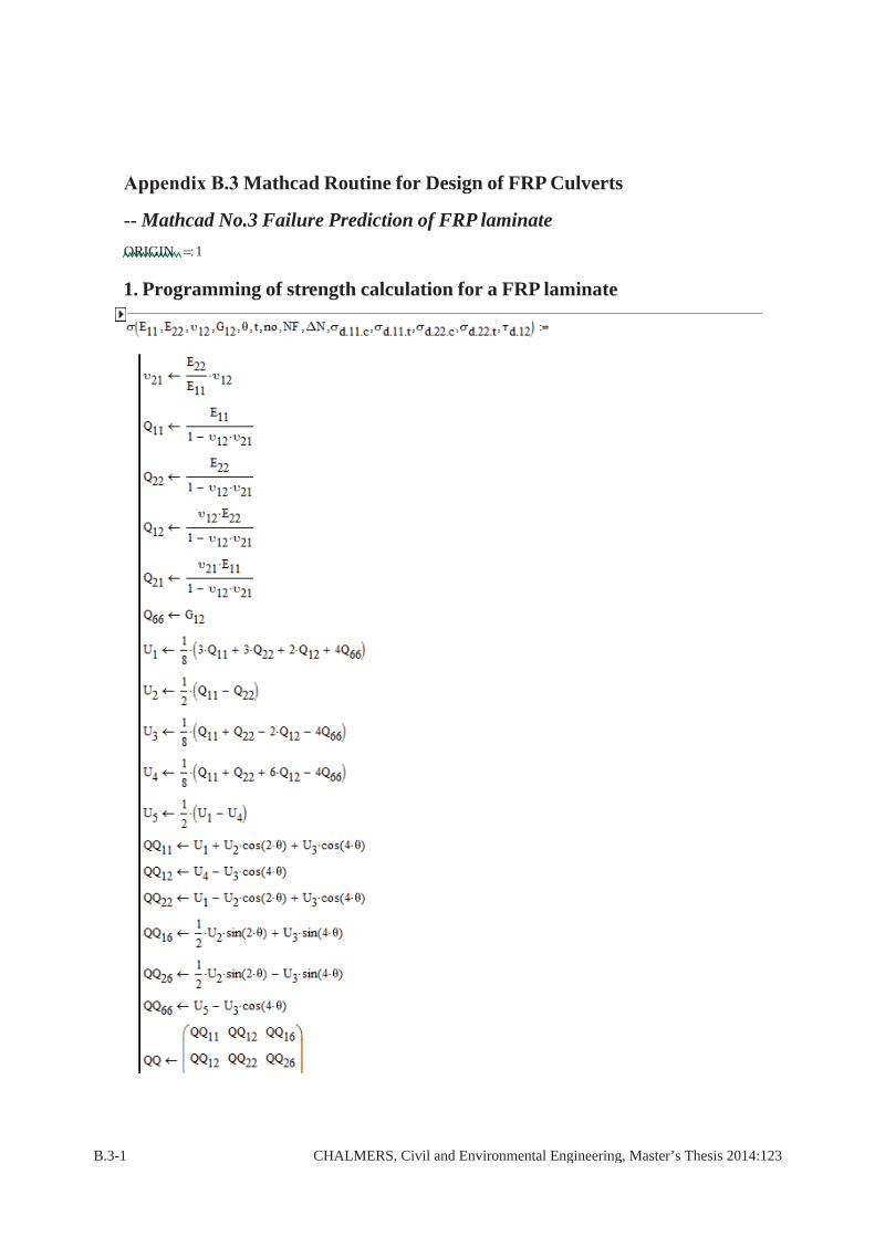
Mathcad Routine for Design of FRP Culverts
-- Mathcad No.3 Failure Prediction of FRP laminateORIGIN 1
1. Programming of strength calculation for a FRP laminate
B.3-1 CHALMERS, Civil and Environmental Engineering, Master’s Thesis 2014:123

CHALMERS, Civil and Environmental Engineering, Master’s Thesis 2014:123 B.3-2
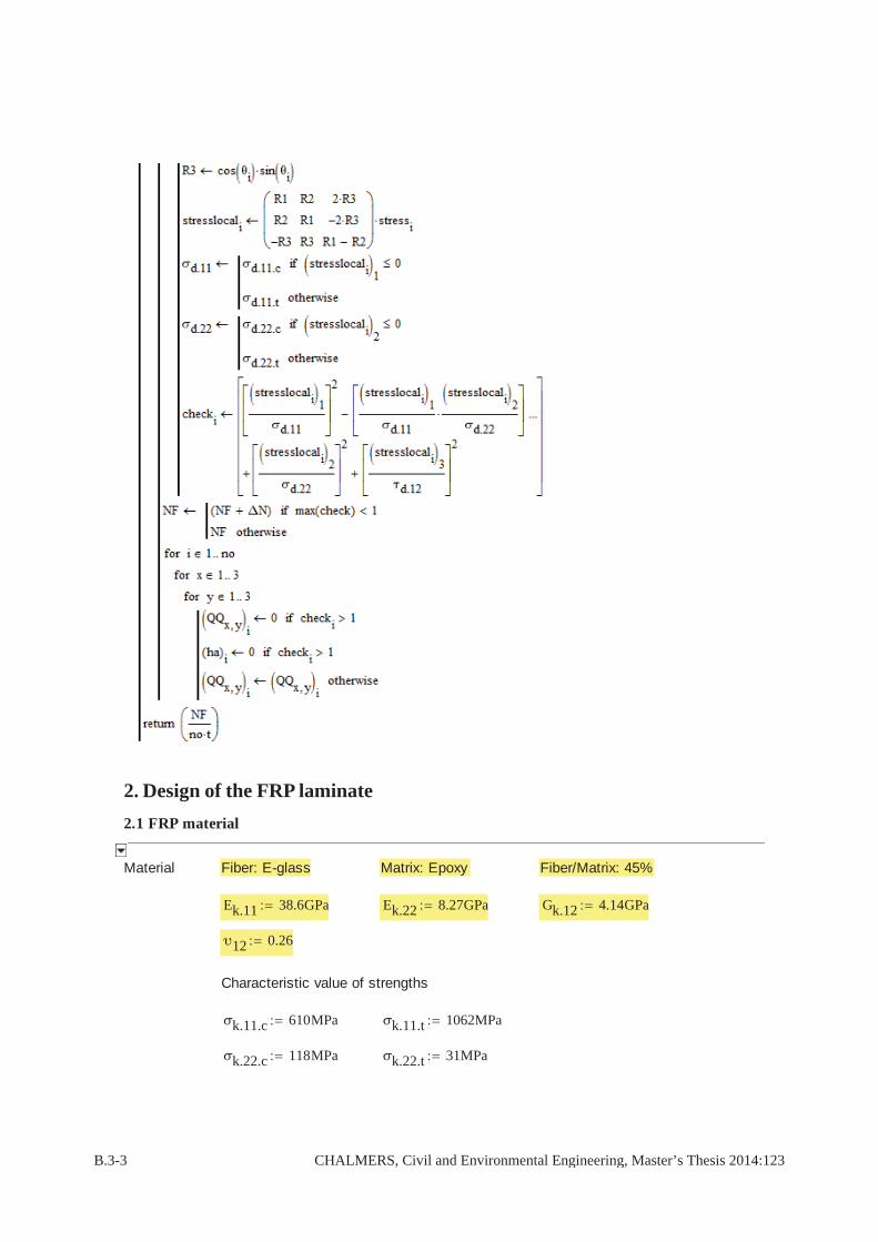
2. Design of the FRP laminate
2.1 FRP material
Material Fiber: E-glass Matrix: Epoxy Fiber/Matrix: 45%
Ek.11 38.6GPa Ek.22 8.27GPa Gk.12 4.14GPa
υ12 0.26
Characteristic value of strengths
σk.11.c 610MPa σk.11.t 1062MPa
σk.22.c 118MPa σk.22.t 31MPa
B.3-3 CHALMERS, Civil and Environmental Engineering, Master’s Thesis 2014:123
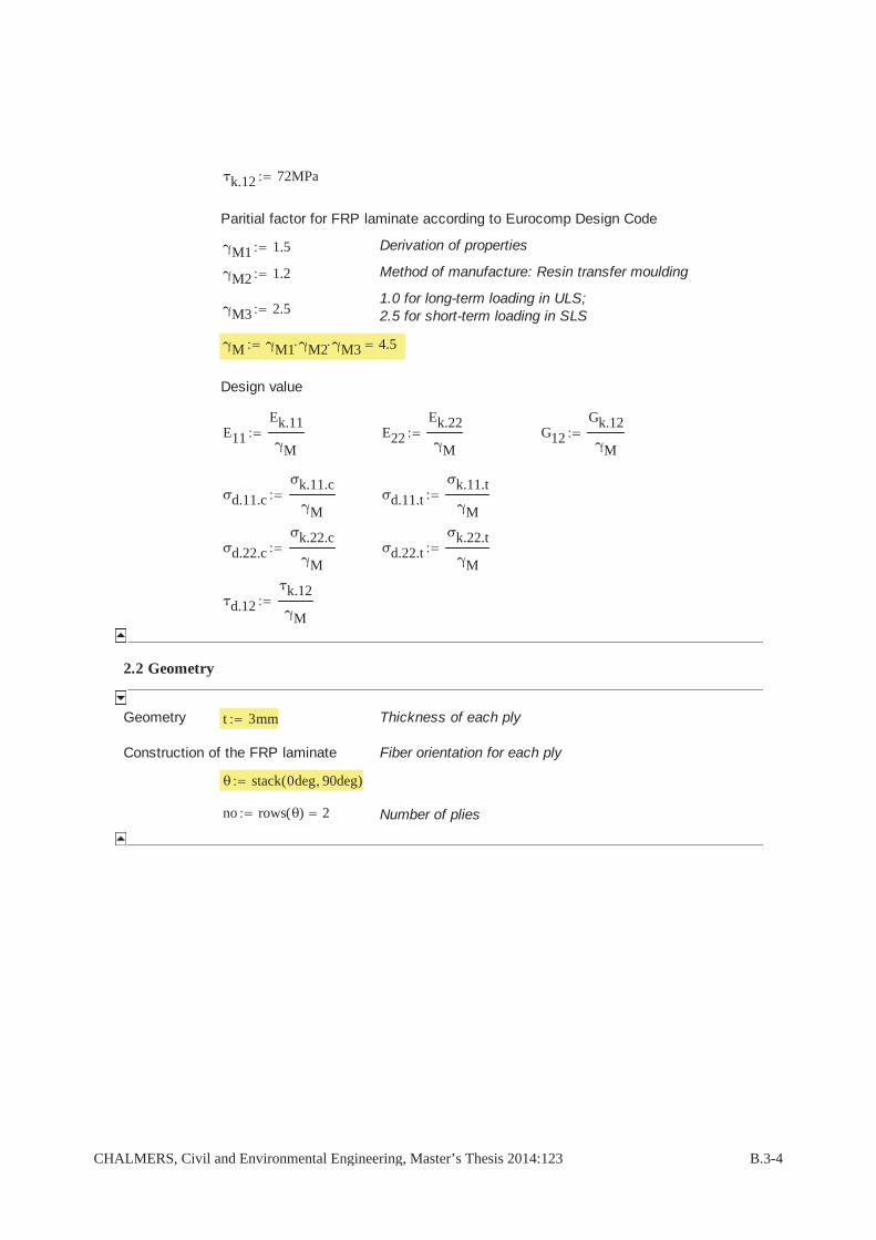
τk.12 72MPa
Paritial factor for FRP laminate according to Eurocomp Design Code
γM1 1.5 Derivation of properties
γM2 1.2 Method of manufacture: Resin transfer moulding
1.0 for long-term loading in ULS;2.5 for short-term loading in SLSγM3 2.5
γM γM1 γM2 γM3 4.5
Design value
E11
Ek.11
γME22
Ek.22
γMG12
Gk.12
γM
σd.11.c
σk.11.c
γMσd.11.t
σk.11.t
γM
σd.22.c
σk.22.c
γMσd.22.t
σk.22.t
γM
τd.12
τk.12
γM
2.2 Geometry
Geometry t 3mm Thickness of each ply
Construction of the FRP laminate Fiber orientation for each ply
θ stack 0deg 90deg( )
no rows θ( ) 2 Number of plies
CHALMERS, Civil and Environmental Engineering, Master’s Thesis 2014:123 B.3-4

3. Ultimate strength of the designed laminate
Assume a proper value of applied normal force with certain increment
N.xx N.yyN.xy
ΔN
5
0
0
kN
mPositive value for tensile forcesNegative value for compressive forcesNF
20
0
0
kN
m
σ E11 E22 υ12 G12 θ t no NF ΔN σd.11.c σd.11.t σd.22.c σd.22.t τd.12
118.333
0
0
MPa
B.3-5 CHALMERS, Civil and Environmental Engineering, Master’s Thesis 2014:123

CHALMERS, Civil and Environmental Engineering, Master’s Thesis 2014:123 B.4-1
Appendix B.4 Data for the FE analysis of FRP culverts in ABAQUS
Dimension of the model
Figure B.4-1 Dimension of the surrounding soil material
Figure B.4-2 Dimension of the Box Culvert structure (same for both Case 14 and 15)
hc – height of soil cover 0.75 meter for Case 14 1.0 meter for Case 15
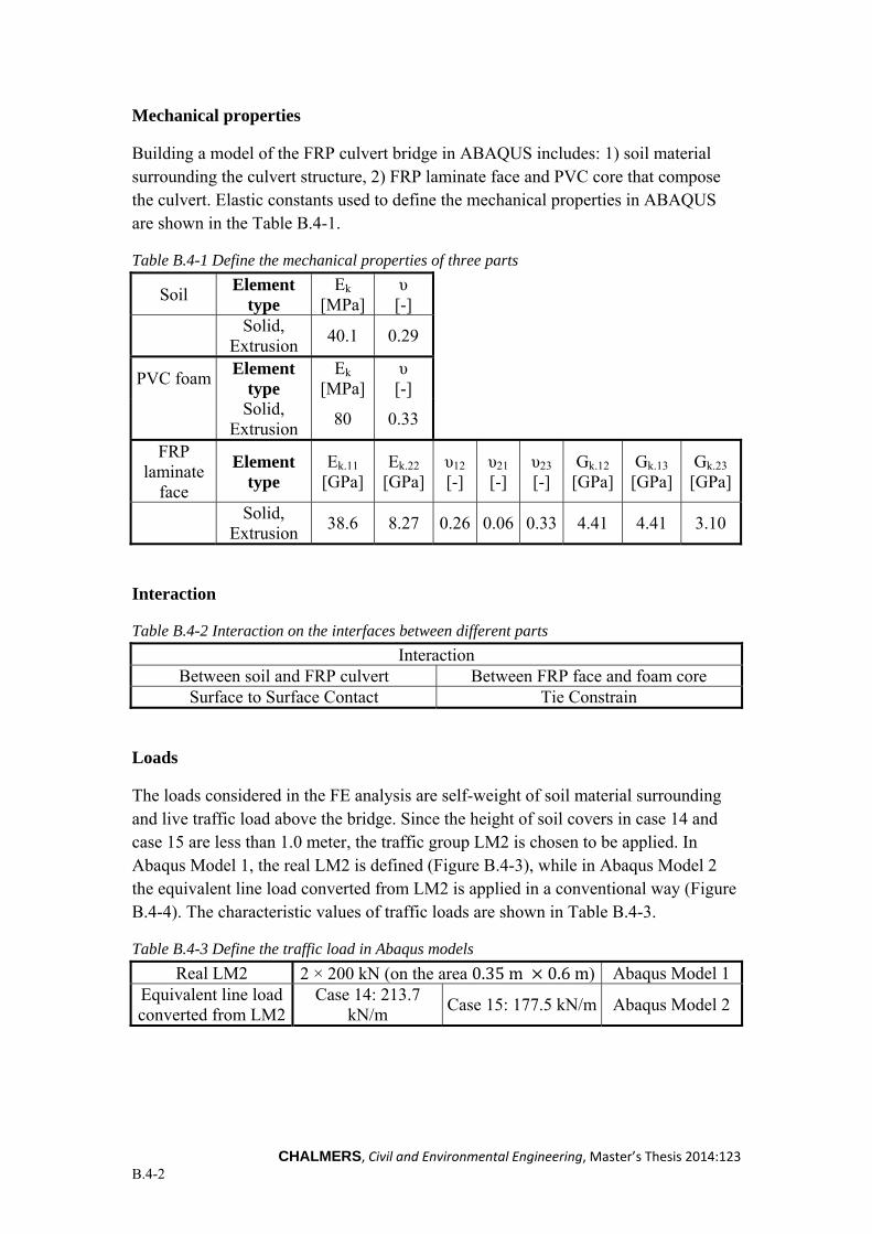
CHALMERS, Civil and Environmental Engineering, Master’s Thesis 2014:123 B.4-2
Mechanical properties
Building a model of the FRP culvert bridge in ABAQUS includes: 1) soil material surrounding the culvert structure, 2) FRP laminate face and PVC core that compose the culvert. Elastic constants used to define the mechanical properties in ABAQUS are shown in the Table B.4-1.
Table B.4-1 Define the mechanical properties of three parts
Soil Element
type Ek
[MPa]υ
[-]
Solid,
Extrusion 40.1 0.29
PVC foam Element
type Ek
[MPa]υ
[-]
Solid,
Extrusion 80 0.33
FRP laminate
face
Element type
Ek.11
[GPa] Ek.22
[GPa]υ12
[-] υ21
[-] υ23
[-] Gk.12
[GPa]Gk.13
[GPa] Gk.23
[GPa]
Solid,
Extrusion 38.6 8.27 0.26 0.06 0.33 4.41 4.41 3.10
Interaction
Table B.4-2 Interaction on the interfaces between different parts
Interaction Between soil and FRP culvert Between FRP face and foam core
Surface to Surface Contact Tie Constrain
Loads
The loads considered in the FE analysis are self-weight of soil material surrounding and live traffic load above the bridge. Since the height of soil covers in case 14 and case 15 are less than 1.0 meter, the traffic group LM2 is chosen to be applied. In Abaqus Model 1, the real LM2 is defined (Figure B.4-3), while in Abaqus Model 2 the equivalent line load converted from LM2 is applied in a conventional way (Figure B.4-4). The characteristic values of traffic loads are shown in Table B.4-3.
Table B.4-3 Define the traffic load in Abaqus models
Real LM2 2 × 200 kN (on the area 0.35 m 0.6 m) Abaqus Model 1 Equivalent line load converted from LM2
Case 14: 213.7 kN/m
Case 15: 177.5 kN/m Abaqus Model 2
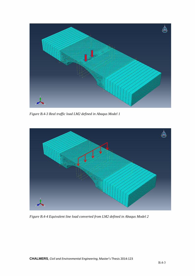
CHALMERS, Civil and Environmental Engineering, Master’s Thesis 2014:123 B.4-3
Figure B.4-3 Real traffic load LM2 defined in Abaqus Model 1
Figure B.4-4 Equivalent line load converted from LM2 defined in Abaqus Model 2
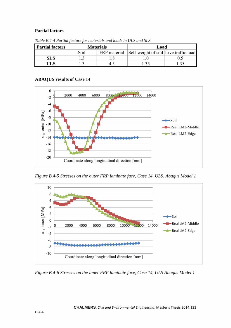
CHALMERS, Civil and Environmental Engineering, Master’s Thesis 2014:123 B.4-4
Partial factors
Table B.4-4 Partial factors for materials and loads in ULS and SLS
Partial factors Materials Load Soil FRP material Self-weight of soil Live traffic load
SLS 1.3 1.8 1.0 0.5 ULS 1.3 4.5 1.35 1.35
ABAQUS results of Case 14
Figure B.4-5 Stresses on the outer FRP laminate face, Case 14, ULS, Abaqus Model 1
Figure B.4-6 Stresses on the inner FRP laminate face, Case 14, ULS Abaqus Model 1
-20
-18
-16
-14
-12
-10
-8
-6
-4
-2
00 2000 4000 6000 8000 10000 12000 14000
σ 11-
oute
r [M
Pa]
Coordinate along longitudinal direction [mm]
Soil
Real LM2-Middle
Real LM2-Edge
‐10
‐8
‐6
‐4
‐2
0
2
4
6
8
10
0 2000 4000 6000 8000 10000 12000 14000
σ 11-
inne
r [M
Pa]
Coordinate along longitudinal direction [mm]
Soil
Real LM2‐Middle
Real LM2‐Edge
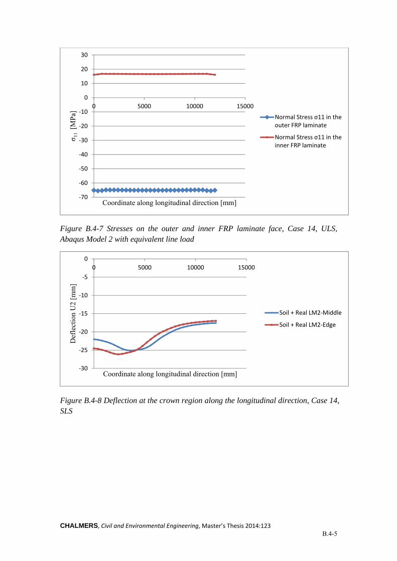
CHALMERS, Civil and Environmental Engineering, Master’s Thesis 2014:123 B.4-5
Figure B.4-7 Stresses on the outer and inner FRP laminate face, Case 14, ULS, Abaqus Model 2 with equivalent line load
Figure B.4-8 Deflection at the crown region along the longitudinal direction, Case 14, SLS
‐70
‐60
‐50
‐40
‐30
‐20
‐10
0
10
20
30
0 5000 10000 15000
σ 11
[M
Pa]
Coordinate along longitudinal direction [mm]
Normal Stress σ11 in the outer FRP laminate
Normal Stress σ11 in the inner FRP laminate
‐30
‐25
‐20
‐15
‐10
‐5
0
0 5000 10000 15000
Def
lect
ion
U2
[mm
]
Coordinate along longitudinal direction [mm]
Soil + Real LM2‐Middle
Soil + Real LM2‐Edge

CHALMERS, Civil and Environmental Engineering, Master’s Thesis 2014:123 B.4-6
ABAQUS results of Case 15
Figure B.4-9 Stresses on the outer FRP laminate face, Case 15, ULS, Abaqus Model 1
Figure B.4-10 Stresses on the inner FRP laminate face, Case 15, ULS, Abaqus Model 1
-20
-18
-16
-14
-12
-10
-8
-6
-4
-2
00 2000 4000 6000 8000 10000 12000 14000
σ 11-
oute
r [M
Pa]
Coordinate along longitudinal direction [mm]
Soil
Real LM2-Middle
Real LM2-Edge
‐8
‐6
‐4
‐2
0
2
4
6
8
0 2000 4000 6000 8000 10000 12000 14000
σ 11-
inne
r [M
Pa]
Coordinate along longitudinal direction [mm]
Soil
Real LM2‐Middle
Real LM2‐Edge
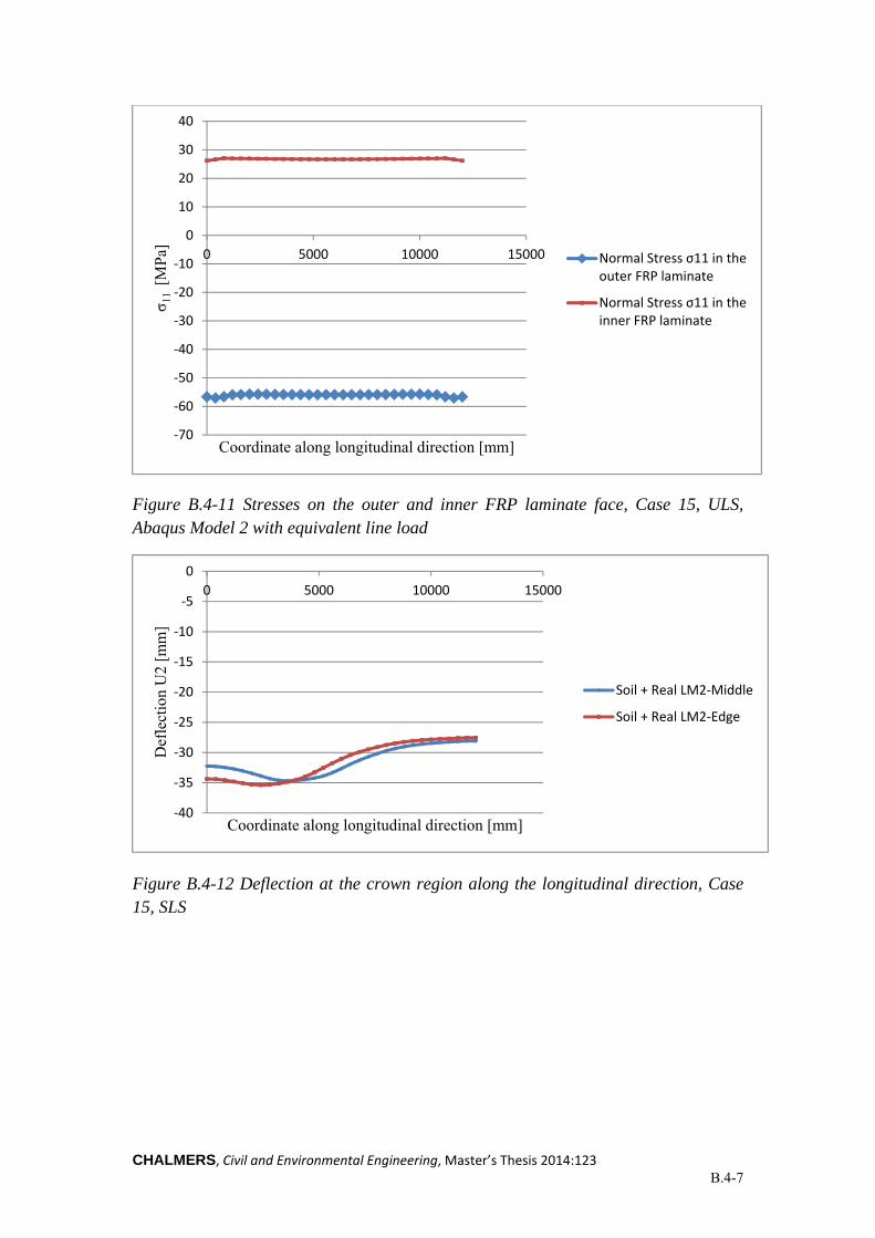
CHALMERS, Civil and Environmental Engineering, Master’s Thesis 2014:123 B.4-7
Figure B.4-11 Stresses on the outer and inner FRP laminate face, Case 15, ULS, Abaqus Model 2 with equivalent line load
Figure B.4-12 Deflection at the crown region along the longitudinal direction, Case 15, SLS
‐70
‐60
‐50
‐40
‐30
‐20
‐10
0
10
20
30
40
0 5000 10000 15000
σ 11
[M
Pa]
Coordinate along longitudinal direction [mm]
Normal Stress σ11 in the outer FRP laminate
Normal Stress σ11 in the inner FRP laminate
‐40
‐35
‐30
‐25
‐20
‐15
‐10
‐5
0
0 5000 10000 15000
Def
lect
ion
U2
[mm
]
Coordinate along longitudinal direction [mm]
Soil + Real LM2‐Middle
Soil + Real LM2‐Edge
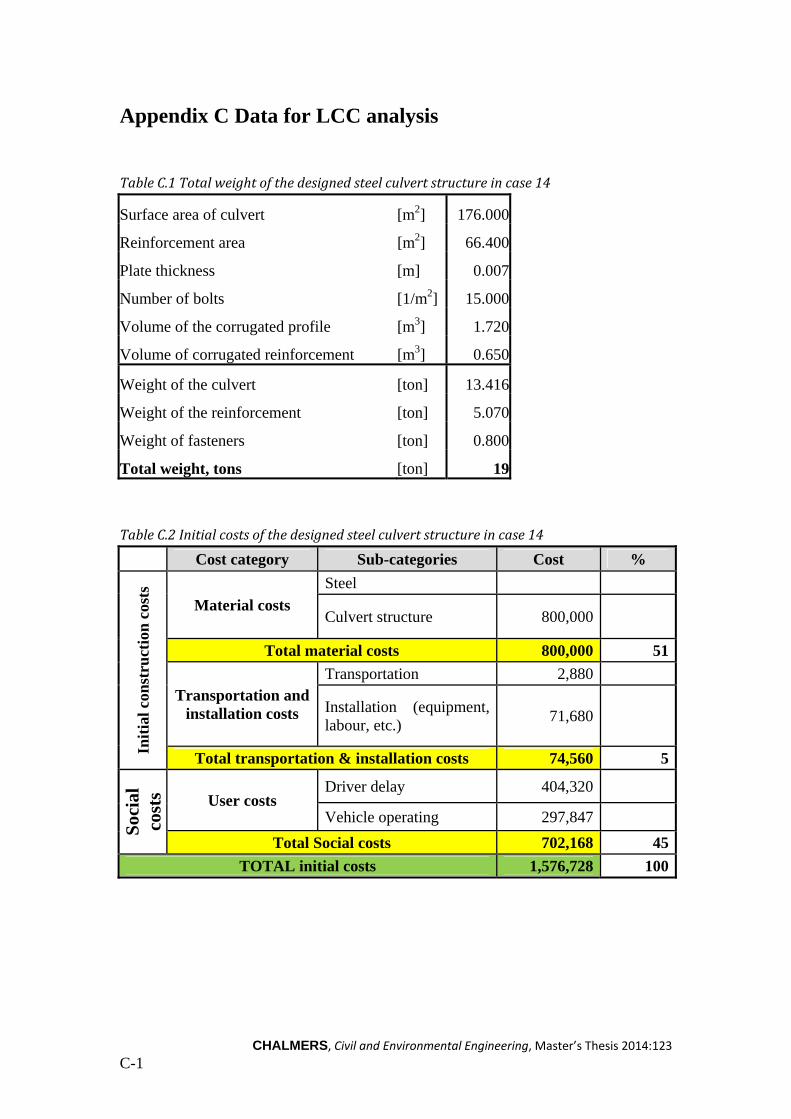
CHALMERS, Civil and Environmental Engineering, Master’s Thesis 2014:123
C-1
Appendix C Data for LCC analysis
TableC.1Totalweightofthedesignedsteelculvertstructureincase14
Surface area of culvert [m2] 176.000
Reinforcement area [m2] 66.400
Plate thickness [m] 0.007
Number of bolts [1/m2] 15.000
Volume of the corrugated profile [m3] 1.720
Volume of corrugated reinforcement [m3] 0.650
Weight of the culvert [ton] 13.416
Weight of the reinforcement [ton] 5.070
Weight of fasteners [ton] 0.800
Total weight, tons [ton] 19
TableC.2Initialcostsofthedesignedsteelculvertstructureincase14
Cost category Sub-categories Cost %
Init
ial c
onst
ruct
ion
cos
ts
Material costs
Steel
Culvert structure 800,000
Total material costs 800,000 51
Transportation and installation costs
Transportation 2,880
Installation (equipment, labour, etc.)
71,680
Total transportation & installation costs 74,560 5
Soc
ial
cost
s User costs Driver delay 404,320
Vehicle operating 297,847
Total Social costs 702,168 45
TOTAL initial costs 1,576,728 100

CHALMERS, Civil and Environmental Engineering, Master’s Thesis 2014:123
C-2
TableC.3TotalweightofthedesignedFRPculvertstructureincase14
Surface area of culvert [m2] 180.000
Area of foam in cross-section [m2] 4.200
Area of laminates in cross-section [m2] 0.270
Volume of the foam [m3] 50.400
Number of laminate's layers [-] 9.000
One lamina's thickness [m] 0.001
Volume fracture [-] 0.450
Area of the top mould [m2] 23.000
Area of the bottom mould [m2] 22.000
Amount of epoxy in top skin [litre] 910.800
Amount of epoxy in bottom skin [litre] 871.200
Number of fasteners [-] 500.000
Weight of the structure [ton] 9.86
Weight of the fasteners [ton] 0.11
Total weight [ton] 10
TableC.4.InitialcostsofthedesignedFRPculvertstructureincase14
Cost category Sub-categories Cost [SEK] %
Init
ial c
onst
ruct
ion
cos
ts
Material costs
FRP sandwich
Moulds 26,960
Sandwich assembly 57,600
E-glass fibres 38,880
Epoxy resin 178,200
Foam 241,920
FRP fasteners 65,000
Total material 608,560 44
Transportation and installation costs
Transportation 720
Installation (equipment, labour, etc.) 71,680
Total transportation & installation costs 72,400 5
Soc
ial
cost
s Driver delay 404,368
Vehicle operating 297,704
Total Social costs 702,072 51
TOTAL initial costs 1,383,032 100

CHALMERS, Civil and Environmental Engineering, Master’s Thesis 2014:123
C-3
TableC.5.Maintenance&operationcosts
Maintenance & repair Quantity [m2]
Cost [SEK/m2]
Cost [SEK]
LCC cost
Steel
M&R expenses per year 176 30 5,280
M&R every 15 year 176 60,812
Total life-cycle cost 83,223
FRP culvert
Life-cycle expenses, 10% ofsteel 8,322
TableC.6Demolitioncosts
Cost categories Cost LCC cost
Steel
Demounting (labour, equipment, etc.) 71,680 4,573
Transportation of materials, SEK/km 2,880 184
Waste disposal, SEK -8,717 -556
Total 65,843 4,200
FRP
Demounting (labour, equipment, etc.) 71,680 4,573
Transportation of materials, SEK/km 720 46
Waste disposal, SEK -11,271 -719
Total 61,129 3,900
TableC.7Summaryoftheresults
Comparison Steel % FRP % Saving [%]
Initial
Material 800,000 608,560 31
Installation & transport 74,560 72,400
Social 702,168 702,072
Total 1,576,728 95 1,383,032 99 14
M&R Maintenance & repair 83,223 5 8,322 1 90
End of life Disposal 4,200 0 3,900 0
TOTAL 1,664,151 100 1,395,254 100 19
Top Related