


Languages
Pages
Legal


Analysis and optimisation of video transmission in
LTE networks
Marco António Martins Castanho
Thesis to obtain the Master of Science Degree in
Electrical and Computer Engineering
Supervisor: Prof. Luís Manuel de Jesus Sousa Correia
Examination Committee
Chairperson: Prof. José Eduardo Charters Ribeiro da Cunha Sanguino
Supervisor: Prof. Luís Manuel de Jesus Sousa Correia
Members of Committee: Prof. Paulo Lobato Correia
Eng. Ricardo Dinis
February 2015

ii

iii
To my family

iv

v
Acknowledgements
Acknowledgements
I would like to start by expressing my deep gratitude to Professor Luís M. Correia, first for trusting me
with this thesis and, consequently, allowing me to do this work in collaboration with a major
telecommunications operator, which proved to be a gratifying experience and an excellent opportunity
to have a close look at real engineering work, before becoming an engineer myself, and second, for all
the guidance, support and patience, without which I would not had been able to do this work. I would
also like to thank to all Group for Research on Wireless (GROW) members, for the opinions and
suggestions given during the presentations performed, and especially, I would like to thank the support
provided by Michal Mackowiak, who helped me defining the right path to follow in the troubled beginning
of this work, and by Lúcio Ferreira, without whom I would still be trying to understand the simulator by
the time I am writing these acknowledgements.
Next, I would like to thank NOS Comunicações (formerly Optimus Telecomunicações), in special to Eng.
Ricardo Dinis, for all the help and technical support throughout the development of this thesis.
A special thanks to Professor João Ascenso, for his availability and for the information supplied
regarding the video quality estimation models used in this thesis.
For all the good company, support and amusement, I would like to thank all my friends from
Casa do Povo, especially Miguel Rodrigues, Diogo Monteiro, António Maciel and Ricardo Francisco.
Never forgetting all my friends from my hometown, Caia, to whom I am very thankful for all the short,
but very well-spent time.
A very special thanks to my aunt Armandina and uncle Joaquim, for all the support and care during and
after the time I lived with them. I am also very thankful to my Grandparents and to all my family.
My final but most important thanks go to my Father, Mother and Sister, for all the love and
encouragement, and whose unconditional support was crucial for me in achieving this goal.

vi

vii
Abstract
Abstract
This dissertation focuses on the study of video transmission over Long Term Evolution (LTE), more
specifically on the evolved Multimedia Broadcast Multicast Service (eMBMS). The service is assessed
in terms of user satisfaction, analysing the video quality perceived by the user and the probability of the
video playback to stop, both these metrics being based on the packet loss ratio. Several parametric
scenarios are tested, where the influence of each parameter on the performance metrics is assessed.
One of these parametric scenarios assesses the influence of Multimedia Broadcast Single Frequency
Network (MBSFN) being enabled or disabled based on its main properties. Additionally, two realistic
scenarios are tested, based on real urban and rural networks. It is verified that the Quality of Service
(QoS) provided to the user is always better when MBSFN is enabled. Based on the results from the
urban scenario, all outdoor users are expected to be provided with at least an acceptable service. The
coverage for indoor users was initially obtained as 25%, but an extrapolation based on the parametric
results suggests that this value can raise to 91% under more advantageous conditions, such as lower
base frequency and Modulation and Coding Scheme (MCS) index. Measurements performed in an
indoor hotspot evaluate the impact of the MCS index in the performance of this service, and an analysis
is performed on the balance between maximum throughput and coverage. As a low modulation
enhances coverage, therefore serving more users, high modulation increases the maximum throughput,
hence allowing for more simultaneous video streams. Results from simulations and measurements are
compared.
Keywords
LTE, Video Transmission, eMBMS, MBSFN, MCS Index, Coverage.

viii
Resumo
Resumo Esta dissertação foca-se no estudo de transmissão de vídeo sobre LTE, mais especificamente no
serviço evolved Multimedia Broadcast Multicast Service (eMBMS). O serviço é aferido em termos de
satisfação do utilizador, analisando a qualidade de vídeo depreendida pelo utilizador e a probabilidade
de a reprodução do vídeo parar, sendo ambas estas métricas baseadas no rácio de perda de pacotes.
Vários cenários paramétricos são testados, onde a influência de cada parâmetro nas métricas de
desempenho é avaliada. Um destes cenários paramétricos avalia a influência de a MBSFN estar ativada
ou desativada, baseando-se nas suas principais propriedades. Adicionalmente, dois cenários realistas
são testados, baseados em redes reais urbana e rural. Verifica-se que a qualidade de serviço fornecida
ao utilizador é sempre melhor quando a MBSFN está ativada. Com base nos resultados para o cenário
urbano, é esperado que a todos os utilizadores exteriores seja fornecido um serviço no mínimo
aceitável. A cobertura para utilizadores interiores foi inicialmente obtida como 25% mas uma
extrapolação baseada nos resultados paramétricos sugere que este valor possa subir para 91% se em
condições mais vantajosas, tais como frequência base e índice de MCS mais baixos. Medições
realizadas num hotspot interior avaliam o impacto do índice de MCS no desempenho deste serviço, e
a análise é feita como um balanço entre velocidade máxima de transmissão e cobertura. Enquanto uma
modulação baixa melhora a cobertura, servindo assim mais utilizadores, uma modulação mais alta
aumenta a velocidade máxima de transmissão, permitindo mais canais vídeo em simultâneo. Os
resultados das simulações e das medições são comparados.
Palavras-chave
LTE, Transmissão de Vídeo, eMBMS, MBSFN, Índice de MCS, Cobertura.

ix
Table of Contents
Table of Contents
Acknowledgements ................................................................................. v
Abstract ................................................................................................. vii
Resumo ................................................................................................ viii
Table of Contents ................................................................................... ix
List of Figures ........................................................................................ xi
List of Tables ......................................................................................... xiii
List of Acronyms .................................................................................. xiv
List of Symbols .................................................................................... xviii
List of Software .................................................................................... xxi
1 Introduction .................................................................................. 1
1.1 Overview and Motivation ......................................................................... 2
1.2 Contents and Contributions ..................................................................... 5
2 Fundamental Aspects ................................................................... 7
2.1 Long Term Evolution ............................................................................... 8
2.1.1 Network Architecture ............................................................................................. 8
2.1.2 Radio Interface ...................................................................................................... 9
2.1.3 Capacity ............................................................................................................... 13
2.2 Services and Applications...................................................................... 15
2.3 Video Transmission ............................................................................... 17
2.4 Evolved Multimedia Broadcast Multicast Service .................................. 21
2.5 Performance Parameters....................................................................... 24
2.6 State of the Art ....................................................................................... 25
3 Models and Simulator Description .............................................. 29
3.1 LTE Network Simulator .......................................................................... 30
3.2 Radio Link Model ................................................................................... 32

x
3.3 Video Quality Assessment Models ........................................................ 34
3.4 Leaky Bucket Model .............................................................................. 36
3.5 Global Model Simulator ......................................................................... 37
3.5.1 Simulator set up ................................................................................................... 38
3.5.2 Video Quality Models ........................................................................................... 40
3.5.3 Rebuffering Delay Models ................................................................................... 41
3.6 Models and Simulator Assessment ....................................................... 43
4 Results Assessment ................................................................... 49
4.1 Scenarios Description ............................................................................ 50
4.2 Results Analysis .................................................................................... 58
4.3 Measurements ....................................................................................... 68
4.3.1 Procedure ............................................................................................................ 68
4.3.2 Results ................................................................................................................. 71
4.4 Comparison of Simulation and Measurement results ............................ 75
5 Conclusions ................................................................................ 79
Annex A. Link Budget ......................................................................... 85
Annex B. COST 231Walfisch-Ikegami Model ..................................... 89
Annex C. M.2135 Propagation Models ............................................... 93
C.1 Urban Microcell (UMi) ............................................................................ 94
C.2 Rural Macrocell (RMa) ........................................................................... 96
Annex D. Coefficients for ITU-T G.1070 Model ................................... 99
Annex E. Additional Simulation Results ............................................ 103
E.1 Additional results from parametric and realistic scenarios ................... 104
E.2 Results for comparison with the measurements .................................. 107
Annex F. Additional Measurements Results ..................................... 109
F.1 SINR vs. MCS index ............................................................................ 110
F.2 RSRP vs. MCS index .......................................................................... 111
References.......................................................................................... 113

xi
List of Figures
List of Figures Figure 1.1. Evolution of 3GPP releases for mobile technologies (adapted from [AT4W11]). ....... 3
Figure 1.2. Expected global mobile data traffic per service, 2013 to 2018 (adapted from [Cisc14b]). ............................................................................................................................. 4
Figure 1.3. Expected global mobile devices and connections growth, 2013-2018 (adapted from [Cisc14b]). ............................................................................................................ 4
Figure 2.1. The EPS Network with the eMBMS reference architecture (adapted from [AlcL09] and [Sams13]). ............................................................................................................ 8
Figure 2.2. Functional Split between E-UTRAN and EPC (adapted from [AlcL09]) ...................... 9
Figure 2.3. Type 1 Frame Structure (adapted from [Anri09]) ...................................................... 10
Figure 2.4. Relationship between a slot, symbols and RBs (adapted from [Anri09]). ................. 11
Figure 2.5. Diagram of a DL frame (adapted from [Anri09]). ....................................................... 12
Figure 2.6. Global architecture of video system (adapted from [FaPe09]) ................................. 18
Figure 2.7. Types of pictures coded in a data stream (adapted from [FaPe09]). ........................ 19
Figure 2.8. Broadcast versus Unicast (extracted from [Eric13]). ................................................. 22
Figure 2.9. MBMS Session Start Procedure (extracted from [3GPP11a]). ................................. 23
Figure 2.10. SFN principles (extracted from [Eric13]). ................................................................ 23
Figure 3.1. Example of a default eMBMS scenario. .................................................................... 30
Figure 3.2. Examples of attributes edition for two network elements of a pre-defined scenario. 31
Figure 3.3. Example of available results from the OPNET simulation Results Browser. ............ 31
Figure 3.4. Example of network simulation results, in this case showing the received throughput over the simulation time for a specific UE in several simulation runs. ............... 32
Figure 3.5. Leaky bucket bounds in the VBR case (extracted from [RiCh03]). ........................... 37
Figure 3.6. Simulation overview and input/output files (module developed by the author of this thesis highlighted in blue). ................................................................................. 38
Figure 3.7. Simulator set up for Model Assessment. .................................................................. 39
Figure 3.8. Illustration of peak bit rate 𝑅 and buffer size 𝐵 values for the test bit stream. .......... 41
Figure 3.9. Average and standard deviations of the MOS at the UE for varying number of simulations. ........................................................................................................ 44
Figure 3.10. Influence of the distance between eNBs in the MOS. ............................................ 45
Figure 3.11. Probability of user satisfaction according to distance to 1st eNB as an assessment of the delay models. ........................................................................................... 46
Figure 3.12. Influence of constructive or destructive interference resulting from MBSFN being enabled or disabled, respectively. ..................................................................... 46
Figure 4.1. Reference Scenario. ................................................................................................. 50
Figure 4.2. 37-cell parametric scenarios configuration. .............................................................. 54
Figure 4.3. Realistic Urban scenario configuration (coordinates are represented in meters). .... 56
Figure 4.4. Realistic Rural scenario configuration (coordinates are represented in meters). ..... 57
Figure 4.5. MOS results for scenario 1. ....................................................................................... 59
Figure 4.6. MOS results for scenario 2. ....................................................................................... 60
Figure 4.7. MOS results for scenario 3. ....................................................................................... 61
Figure 4.8. MOS results for scenario 4. ....................................................................................... 62
Figure 4.9. MOS results for scenario 5. ....................................................................................... 63

xii
Figure 4.10. MOS results for scenario 6. ..................................................................................... 64
Figure 4.11. MOS results for scenario 7. ..................................................................................... 64
Figure 4.12. MOS results for Realistic Urban scenario. .............................................................. 65
Figure 4.13. MOS results for Realistic Rural scenario. ............................................................... 67
Figure 4.14. Approximate building plan with BSs locations and measurement positions ........... 69
Figure 4.15. MOS vs. SNR figures, with logistic trend lines, for five different MCS indexes. ..... 73
Figure 4.16. Logistic trend lines for the measurements results................................................... 73
Figure 4.17. Influence of the SNR in the received throughput. ................................................... 75
Figure 4.18. Relation between the received throughput and the MOS. ...................................... 75
Figure 4.19. Logistic trend lines for the simulations results. ....................................................... 76
Figure B.1. Definition of parameters for use in COST 231 Walfisch-Ikegami propagation model (adapted from [Corr12]). .................................................................................... 90
Figure C.1. Geometry for 𝑑1 and 𝑑2 path-loss model (extracted from [ITUR09]). ...................... 95
Figure E.1. User satisfaction results for scenario 1. .................................................................. 104
Figure E.2. User satisfaction results for scenario 2. .................................................................. 104
Figure E.3. User satisfaction results for scenario 3. .................................................................. 104
Figure E.4. User satisfaction results for scenario 4. .................................................................. 105
Figure E.5. User satisfaction results for scenario 5. .................................................................. 105
Figure E.6. User satisfaction results for scenario 6. .................................................................. 105
Figure E.7. User satisfaction results for scenario 8. .................................................................. 105
Figure E.8. User satisfaction results for Realistic Urban scenario – UEs stopped. .................. 106
Figure E.9. User satisfaction results for Realistic Urban scenario – UEs moving. .................... 106
Figure E.10. User satisfaction results for Realistic Rural scenario – UEs stopped. .................. 106
Figure E.11. User satisfaction results for Realistic Rural scenario – UEs moving. ................... 106
Figure E.12. MOS vs. SNR figures, with logistic trend lines, for five different MCS indexes. ... 108
Figure E.13. MOS vs. UE-BS distance figure, with logistic trend lines, for five MCS indexes. . 108
Figure F.1. Intervals of SINR [dB] that assures a certain MOS for each MCS index. ............... 110
Figure F.2. Intervals of RSRP [dBm] that assures a certain MOS for each MCS index. .......... 111
xiii
List of Tables
List of Tables Table 2.1. Key parameters for different bandwidths (adapted from [HoTo07]). .......................... 11
Table 2.2. DL peak data rates (extracted from [HoTo07]). .......................................................... 14
Table 2.3. UL peak data rates (extracted from [HoTo07]). .......................................................... 14
Table 2.4. LTE service classes (adapted from [3GPP06b]) ........................................................ 16
Table 3.1. Optimal values for 𝑥1, 𝑥2 and 𝑘 (extracted from [JoSo14]) ........................................ 36
Table 3.2. Video trace files parameters (extracted from [ASU14]).............................................. 39
Table 4.1. Reference scenario parameters. ................................................................................ 50
Table 4.2. Parameters values for scenario 1............................................................................... 51
Table 4.3. Parameters values for scenario 2............................................................................... 52
Table 4.4. Parameters values for scenario 3 – UE stopped. ....................................................... 52
Table 4.5. Parameters values for scenario 3 – UE moving. ........................................................ 53
Table 4.6. Parameters values for scenario 4............................................................................... 53
Table 4.7. Parameters values for scenario 5............................................................................... 53
Table 4.8. Parameters values for scenario 6............................................................................... 55
Table 4.9. Parameters values for scenario 7............................................................................... 55
Table 4.10. Parameters values for real urban scenario. ............................................................. 57
Table 4.11. Parameters values for real rural scenario. ............................................................... 58
Table 4.12. MOS scale and evaluation criteria............................................................................ 69
Table 4.13. Modulation, TBS index, Throughput and number of channels. ................................ 70
Table 4.14. MOS for each MCS index and at each building floor. .............................................. 74
Table D.1. Conditions for deriving coefficient tables (extracted from [ITUT07]). ...................... 100
Table D.2. Coefficient table for the video quality estimation function (adapted from [ITUT07]). ......................................................................................................... 100

xiv
List of Acronyms
List of Acronyms 1G First-Generation mobile systems
2G Second-Generation mobile systems
3G Third-Generation mobile systems
3GPP 3rd Generation Partnership Project
4G Fourth-Generation mobile systems
AIPN All-IP Network
AL-FEC Application-Level Forward Erasure Correction
AMC Adaptive Modulation and Coding
AN Access Network
ANACOM Autoridade Nacional de Comunicações
ARQ Automatic Repeat reQuest
AVC Advanced Video Coding
BBU Baseband Unit
BER Bit Error Ratio
BM-SC Broadcast Multicast Serving Centre
BS Base Station
CABAC Context Adaptive Binary Arithmetic Coding
CAVLC Context Adaptive Variable Length Coding
CBR Constant Bit Rate
CDMA Code-Division Multiple Access
CIF Common Intermediate Format
CN Core Network
COST European Cooperation in Science and Technology
CP Cyclic Prefix
DAS Distributed Antenna System
DCT Discrete Cosine Transform
DFT Discrete Fourier Transform
DL Downlink
EDGE Enhanced Data rates for GSM Evolution
eMBMS evolved MBMS
eNB evolved Node B
EPC Evolved Packet Core
EPS Evolved Packet System
ETSI European Telecommunications Standards Institute

xv
E-UTRAN Evolved UMTS Terrestrial Radio Access Network
FDD Frequency-Division Duplexing
FDMA Frequency-Division Multiple Access
FFT Fast Fourier Transform
FLUTE File Delivery over Unidirectional Transport
FMO Flexible Macroblock Ordering
FR Full Reference
FRExt Fidelity Range Extension
FSMC Finite State Markov Chain
FST Frame Structure Type
FTP File Transfer Protocol
GBR Guaranteed Bit Rate
GOP Group of Pictures
GPRS General Packet Radio Service
GSM Global System for Mobile communications
GUI Graphical User Interface
HHR Half Horizontal Resolution
HRD Hypothetical Reference Decoder
HSDPA High Speed Downlink Packet data Access
HSPA High Speed Packet data Access
HSS Home Subscriber Server
HSUPA High Speed Uplink Packet data Access
IEC International Electrotechnical Commission
IMS IP Multimedia Subsystem
IMT-2000 International Mobile Telecommunications-2000
InH Indoor Hotspot
IP Internet Protocol
ISO International Standards Organisation
ITU-T International Telecommunication Union - Telecommunication standardisation sector
JVT Joint Video Tem
LoS Line of Sight
LTE Long Term Evolution
MAC Media Access Control
MB MacroBlock
MBSFN MBMS over a Single Frequency Network
MBMS Multimedia Broadcast/Multicast Service
MBMS-GW MBMS Gateway
MCE MBMS Coordination Entity
MIMO Multiple Input Multiple Output

xvi
MME Mobility Management Entity
MOS Mean Opinion Score
MPEG Moving Picture Experts Group
MPEG-DASH MPEG Dynamic Adaptive Streaming over HTTP
MPEG-TS MPEG Transport Stream
MT Mobile Terminal
NAL Network Adaptation Layer or Network Abstraction Layer
NAS Network Access Server
NR No Reference
OFDM Orthogonal Frequency-Division Multiplexing
OFDMA Orthogonal Frequency-Division Multiple Access
P2P Peer-to-Peer
PAPR Peak-to-Average Power Ratio
PBCH Physical Broadcast Channel
PC Pearson Correlation
PCEF Policy and Charging Enforcing Function
PCFICH Physical Control Format Indicator Channel
PCM Pulse Code Modulation
PCRF Policy and Charging Rules Function
PDCCH Physical Downlink Control Channel
PDB Packet Delay Budget
PDCP Packet Data Convergence Protocol
PDN Public Data Network
PDSCH Physical Downlink Shared Channel
P-GW PDN Gateway
PER Packet Error Loss Rate
PHY Physical Layer
P-SCH Primary Synchronisation Channel
PSNR Peak SNR
PUCCH Physical Uplink Control Channel
PUSCH Physical Uplink Shared Channel
QAM Quadrature Amplitude Modulation
QCI QoS Class Identifier
QCIF Quarter CIF
QoE Quality of Experience
QoS Quality of Service
QPSK Quadrature Phase-Shift Keying
RAN Radio Access Network
RB Resource Block
RMSE Root Mean Square Error

xvii
RR Reduced Reference
RRM Radio Resource Management
RRU Radio Remote Unit
RS Reference Signal
RSRP Reference Signal Received Power
RSRQ Reference Signal Received Quality
RSSI Received Signal Strength Indicator
RT Real Time
SAE System Architecture Evolution
SC-FDMA Single-Carrier Frequency-Division Multiple Access
SDF Service Data Flow
SDMA Space-Division Multiple Access
SFN Single Frequency Network
S-GW Serving Gateway
SINR Signal-to-Interference-plus-Noise Ratio
SISO Single Input Single Output
SNR Signal-to-Noise Ratio
S-SCH Secondary Synchronisation Channel
SVC Scalable Video Coding
TBS Transport Block Size
TDD Time-Division Duplexing
TCP Transmission Control Protocol
TPM Transition Probability Matrix
UE User Equipment
UL Uplink
UMi Urban Microcell
UMTS Universal Mobile Telecommunications System
VBR Variable Bit Rate
VCEG Video Coding Experts Group
VCL Video Coding Layer
VoD Video on Demand
VoIP Voice over IP
WCDMA Wideband CDMA
WWW World Wide Web

xviii
List of Symbols
List of Symbols
∆ℎ𝐵𝑊𝐼
Vertical distance from the BS to the top of the buildings
∆ℎ𝑀𝑊𝐼
Vertical distance from the MT to the top of the buildings
𝜃 Angle between LoS to the building wall and normal vector to the wall
𝜌𝐼𝑁 Signal-to-Interference-plus-Noise Ratio
𝜌𝑁 Signal-to-Noise Ratio
𝜎𝐿𝑜𝑆 Shadow fading standard deviation in case of LoS
𝜎𝑁𝐿𝑜𝑆 Shadow fading standard deviation in case of NLoS
𝜙 Angle between the incident wave and the street where the MT is in
𝜏𝑇𝑇𝐼 Subframe period
𝐴𝑐𝑜𝑣 Threshold for percentage of satisfied users
𝐴𝑜𝑢𝑡 Rebuffering percentage threshold
𝐵𝑟 Video bit rate
𝑑′𝐵𝑃 Breakpoint distance
𝑑𝑖𝑛 Perpendicular distance from building wall to MT
𝑑𝑜𝑢𝑡 Distance from BS to the building wall
𝐷𝐹𝑟 Frame rate robustness factor
𝐷𝑃𝑝𝑙 Packet loss robustness factor
𝐹𝑟 Video frame rate
𝐺𝑟 Reception antenna gain
𝐺𝑡 Transmission antenna gain
ℎ𝑏 BS height
ℎ′𝑏 Effective BS height
𝐻𝐵𝑊𝐼 Average buildings height
ℎ𝑚 MT height

xix
ℎ′𝑚 Effective MT height
𝐻𝐻264 H.264/AVC transform matrix
𝐼𝑐 Video quality due to encoding
𝐼𝑀𝐶𝑆 Modulation and Coding Scheme index
𝐼𝑂𝑓𝑟 Maximum video quality due to encoding
𝐼𝑝 Video quality due to packet loss
𝑘𝑎𝑊𝐼
Loss for BS antennas below the rooftops of the adjacent buildings
𝑘𝑑𝑊𝐼
Dependence of the multiscreen diffraction loss versus distance
𝑘𝑓𝑊𝐼
Dependence of the multiscreen diffraction loss versus frequency
𝐿0 Free space path loss
𝐿𝑏𝑈𝑀𝑖 Basic path loss
𝐿𝐵𝐼𝑈𝑀𝑖 Path loss from UMi outdoor scenario
𝐿𝑏𝑠ℎ𝑊𝐼 Loss due to the difference in heights between the buildings and the BS
𝐿𝐶 BS cable loss
𝐿𝑖𝑛𝑈𝑀𝑖 Path loss inside the building
𝐿𝐿𝑜𝑆 Path loss in case of LoS
𝐿𝑚𝑠𝑑𝑊𝐼 Loss due to multiscreen diffraction
𝐿𝑁𝐿𝑜𝑆 Path loss in case of NLoS
𝐿𝑜𝑟𝑖𝑊𝐼 Loss due to street orientation
𝐿𝑂𝑡𝑜𝐼𝑈𝑀𝑖 Path loss in Outdoor-to-Indoor case
𝐿𝑝 Path loss
𝐿𝑝𝑖𝑛𝑑 Indoor penetration margin
𝐿𝑝𝑃𝑟𝑀 Path loss from the propagation model
𝐿𝑟𝑡𝑠𝑊𝐼 Loss due to rooftop diffraction and scatter
𝐿𝑡𝑤𝑈𝑀𝑖 Loss through the building wall
𝐿𝑈 Loss due to user’s body
𝑀𝐹𝐹 Fast fading margin
𝑀𝑝 Power margin
𝑀𝑆𝐹 Slow fading margin

xx
𝑁𝐼 Number of interfering signals at the receiver antenna
𝑁𝑅𝐵 Number of RBs allocated
𝑁𝑠𝑐 Number of sub-carriers
𝑁𝑠𝑐𝑈 Number of sub-carriers allocated to each user
𝑁𝑠𝑡𝑟𝑒𝑎𝑚𝑠 Number of streams
𝑁𝑠𝑦𝑚𝑏𝑠𝑓
Number of symbols per subframe
𝑁𝑈 Number of supported users
𝑂𝑓𝑟 Optimal frame rate
𝑃𝑝𝑙 Video packet loss ratio
𝑃𝑝𝑙 𝐵 B-frame packet loss ratio
𝑃𝑝𝑙 𝐼 I-frame packet loss ratio
𝑃𝑝𝑙 𝑃 P-frame packet loss ratio
𝑃𝑟 Power at the reception antenna
𝑃𝑅𝑥𝐷𝐿 Power at the MT in DL
𝑃𝑅𝑥𝑈𝐿 Power at the BS in UL
𝑃𝑡 Power at the transmission antenna
𝑃𝑡𝐷𝐿 Power fed to the BS antenna in DL
𝑃𝑡𝑈𝐿 Power fed to the MT antenna in UL
𝑃𝑇𝑥 Transmitted output power
𝑝𝑤 Weighted percentage of slice loss
𝑄𝑚 Modulation order
𝑅2 Square of Pearson’s correlation coefficient
𝑅𝑏 Bit rate
𝑅𝑏𝑈 Channel bit rate per user
𝑅𝑐𝑜𝑑 Channel coding rate
𝑉𝑞 Subjective video quality estimation
𝑤𝑆 Average street width
𝑤𝐵 Average building separation

xxi
List of Software
List of Software Microsoft Excel Spreadsheet application.
Microsoft PowerPoint Slide show presentation.
Riverbed OPNET Modeler 17.5 Software tool for network modelling and simulation.
Notepad++ Text and source code editor for Microsoft Windows.

xxii

1
Chapter 1
Introduction
1 Introduction
This chapter gives a brief overview of the thesis. Firstly, an overview of the problem under study is
introduced, and mobile communication systems and their progress history are presented. Secondly,
motivations and objectives to this thesis are brought up. Finally, a brief description of the thesis structure
is provided.

2
1.1 Overview and Motivation
Mobile phones have become essential in our lives and made their own single stand. Once regarded as
luxury, they are now the most indispensable device in our everyday life, replacing old tools and
empowering new ways of communication, such as Twitter or Instagram, through the emergence of
smartphones and tablets. But no matter how advanced these devices are, they are nothing but
uninteresting gadgets if they are not connected to a network. Therefore, the connection and the network
itself have a major importance in mobile communications, with statistics showing that in Europe there
are more mobile services subscriptions than inhabitants, [ANAC13].
The First Generation (1G) of mobile telecommunication systems, introduced in the 1980s, was analogue
and provided only voice. The advantages of digital technology over analogue one culminated in 1G
being replaced everywhere by Second Generation (2G) networks, launched in 1991 with GSM (Global
System for Mobile communications, originally Group Spécial Mobile), developed by the European
Telecommunications Standards Institute (ETSI). GSM allowed new services, such as Short Message
Service (SMS), and was improved over time to include data communications through packet data
transport, via General Packet Radio Services (GPRS) and Enhanced Data rates for GSM Evolution
(EDGE), known as 2.5G and 2.75G, respectively, [3GPP14a].
International Mobile Telecommunications-2000 (IMT-2000) requirements by the International
Telecommunication Union – Radiocommunication Sector (ITU-R) specified Third Generation (3G)
systems, designed for multimedia communication, with higher bit-rates allowing communication with
high-quality images and video, and access to information and services on public and private networks.
Wideband Code Division Multiple Access (WCDMA), created in the 3rd Generation Partnership Project
(3GPP), came as the most widely adopted air interface for these systems, being the radio access
scheme of the Universal Mobile Telephone System (UMTS) network, [HoTo07]. High Speed Packet
Access (HSPA) extended and improved the performance of UMTS by improving the peak bit rate, first
in Downlink (HSDPA) and then in Uplink (HSUPA).
Although marketed as a Fourth Generation (4G) system, Long Term Evolution (LTE) does not satisfy
the technical requirements 3GPP has adopted for its new standard generation, which were originally set
by ITU-R in its IMT-Advanced specification. However, ITU-R later considered this standard as 4G due
to providing a substantial level of improvement in performance and capabilities with respect to previous
3G systems, [ITUR14]. The use of Orthogonal Frequency Division Multiple Access (OFDMA) in
Downlink (DL) and Single-Carrier Frequency-Division Multiple Access (SC-FDMA) in Uplink (UL)
provides orthogonality among users, reducing interference and improving network capacity, [HoTo09].
Although beyond the scope of this thesis, the next step, LTE-Advanced focuses on higher capacity
providing higher bitrates in a cost efficient way and, at the same time, completely fulfilling the
requirements set by ITU for IMT Advanced as a 4G technology, [3GPP14b]. The evolution of the
mentioned technologies and their correspondence with 3GPP Releases are summarised in Figure 1.1.

3
Figure 1.1. Evolution of 3GPP releases for mobile technologies (adapted from [AT4W11]).
Among the motivations for LTE, providing higher data rates, more capacity and better network efficiency,
compared to existing 3GPP networks based on HSPA, in order to cope with the growing number of
users and the evolution of the capabilities of Mobile Terminals (MT), such as smartphones or tablets,
came as a few of the main driving forces. The much higher peak user bit rate and the reduced latency,
relative to previous 3GPP standards, allow for a better user experience in demanding services, such as
Mobile TV. In fact, statistics show that the average mobile connection data rate grew 81% in 2013, with
the number of connected mobile devices reaching approximately 7 billion, i.e., on average one for each
human being in the world, [Cisc14b].
The traffic growth in Figure 1.2 shows that mobile data traffic is expected to grow at a Compound Annual
Growth Rate (CAGR) of 61% between 2013 and 2018. It also shows the influence of Mobile Video
services in data traffic growth, having the highest expected growth rate of any mobile service with an
expected grow at a CAGR of 69% in the next 5 years, [Cisc14b]. In 2012, mobile video traffic exceeded
50% of the global mobile data one for the first time, with 51% of traffic by the end of the year. It is
expected that two-thirds of the global mobile data traffic will be video by 2017, [Cisc13]. This happens
primarily due to the fact that mobile video content has much higher bit rates than other mobile content
types, but also due to the increase in watching video on mobile devices that has accompanied the
proliferation of smartphones and the rising number of new tablets in the market, as shown in Figure 1.3,
with the mentioned devices accounting for almost half of the global connected mobile devices by 2018.
This creates an opportunity for mobile operators to profit from video, rather than just absorbing the effect,
by offering mobile video services that drive new revenues from differentiated service delivery, [Cisc14a].
Also, there is a constant need to increase network capacity, but there is no definite answer for the
growing data traffic demand and operators are adopting a range of solutions to improve the capacity of
their networks.
The multicast standard for LTE, evolved Multimedia Broadcast Multicast Service (eMBMS), allows
multimedia content to be sent once and received by many end users. This distribution mode can be a

4
valuable alternative to unicast when a large number of users is interested in the same content, as an
effective way for service providers to lower cost per bit. For example, during live streaming of major
events or Media on Demand (MoD), unicast must send the same content to every user individually. But
multicast takes advantage of the inherent broadcast qualities of wireless networks to send the video
only once to reach an equal number of end users. In these scenarios, multicast makes more efficient
use of the available spectrum, consuming at most the resources equivalent to that of the
worst-performing link in the sector, [AlcL14]. Bandwidth consumption does not depend on the number
of simultaneous users, but rather on the number of simultaneous channels that the operator wishes to
send. Within the amount of bandwidth earmarked for multicast, operators have full control on the content
to be broadcasted, [Sams13].
Figure 1.2. Expected global mobile data traffic per service, 2013 to 2018 (adapted from [Cisc14b]).
Figure 1.3. Expected global mobile devices and connections growth, 2013-2018 (adapted from
[Cisc14b]).

5
1.2 Contents and Contributions
The main scope of this thesis is to analyse the impact of several parameters in video transmission over
LTE networks, from a user QoE perspective. Although this subject is not fresh, since LTE provides high
bit rates that galvanises the usage of high demanding services, like video streaming, this thesis focuses
mainly on the eMBMS service and its advantages over the primitive unicast transmission. The objective
is to analyse video quality, as perceived by an end user, and to determine the conditions for an
acceptable QoE to be provided.
This thesis was developed in collaboration with NOS, a major Portuguese telecommunications operator.
This partnership proved to be very useful, since a realistic study was possible, and it created the
possibility for measurements of eMBMS in a real network.
The thesis is composed of 5 chapters, the first being the current one, and is organised as follows. In
Chapter 2, a brief overview of LTE fundamental aspects is given. The LTE network architecture is
presented, with the basic functions of each node briefly described. The LTE radio interface is outlined,
with the LTE frequency bands, bandwidths, frame structure and physical channels being described.
Then, a theoretical LTE capacity analysis is made and a classification of LTE services is presented. This
thesis being focused on video transmission, this subject is also brought up in this chapter, with the global
architecture of a video system and the encoding and decoding basics of the H.264 codec being
described. Next, the eMBMS service is described, with its main advantages being pointed out. Finally,
the chapter closes with the state of the art, where studies from the current literature related to the scope
of this thesis are presented.
In Chapter 3, the simulator and models description take place. First the OPNET Modeler simulator is
introduced, followed by a description of the radio link model used in the simulator. Next, the equations
for video quality assessment model used to estimate the MOS are given and the Leaky Bucket Model,
on whose result the rebuffering delay model relays, is described. Afterwards, the global model simulation
is explained, describing the author’s work regarding simulator set-up and implementation of the
mentioned models. Finally, the assessment of the simulator and the models is made.
Chapter 4 starts by describing the scenarios simulated in this thesis, with all parameters and simulator
configurations specified and justified. Afterwards, the results obtained from the simulations of the
described scenarios are presented and analysed. Next, the description, results and results’ analysis of
the measurements made at the NOS headquarters are given. Finally, a brief comparative analysis
between the simulation and the measurements results is made.
Chapter 5 concludes this thesis, with a critical analysis of the results being made, followed by the main
work conclusions obtained. The thesis ends by giving suggestions for future work. After the conclusions
chapter, a set of Annexes is included, containing complementary information to the thesis.

6

7
Chapter 2
Fundamental Aspects and
State of the Art
2 Fundamental Aspects
This chapter provides an overview of LTE, mainly focusing on its video transmission services.
Afterwards, the main aspects of the H.264/AVC standard are brought up. Finally, the state of the art on
the subject of this thesis is presented.

8
2.1 Long Term Evolution
The LTE standard is specified in Release 8, [3GPP09a], and enhanced in Release 9, [3GPP11a], by
3GPP. It was designed to accommodate the increase in mobile data traffic mainly due to applications
such as Video Streaming or Online Gaming.
This section provides an overview of LTE and it is organised as follows: the LTE Network Architecture
is presented in Subsection 2.1.1; in Subsection 2.1.2 key features of the Radio Interface are addressed;
in Subsection 2.1.3 Coverage and Capacity are discussed; finally, in Subsection 2.1.4, some Mobile
Data Services and Applications are presented. This section is based on [AlcL09] and [DaFJ08].
2.1.1 Network Architecture
System Architecture Evolution’s (SAE) network, called Evolved Packet System (EPS), is the Network
Architecture for LTE. It is a simplified all-IP network (AIPN) that, comparing to previous ones, supports
higher throughput and lower latency. Also, it brings better spectrum efficiency and flexibility, and it
provides inter-working with other standards, not necessarily 3GPP ones, such as GSM, UMTS and
CDMA2000, [Remy10].
EPS is composed of Access Networks (ANs) and Core Networks (CNs), called Evolved-UMTS
Terrestrial Radio Access Network (E-UTRAN) and Evolved Packet Core (EPC), respectively. The EPS
architecture is illustrated in Figure 2.1, with the separation between access (on the left) and core (on the
right) networks being represented by a red dash line. Although not represented in the figure, evolved
Node Bs change information between each other via an interface known as “X2”, mainly for handover
purposes. The boxes in dark blue represent network elements specific to eMBMS, being explained
further in Section 2.4.
Figure 2.1. The EPS Network with the eMBMS reference architecture (adapted from [AlcL09] and
[Sams13]).

9
The access network, E-UTRAN, has a flat (non-hierarchical) architecture, opposite to GSM and UMTS
the ones, in which nodes are more complex the closer they are to the top of the hierarchy. Hence, the
main difference in E-UTRAN is that it has only one type of node, the Base Station (BS), designated as
evolved Node B (eNB), which became more “intelligent”, i.e., it is able handle more tasks by itself. All
radio-related functions are under the responsibility of the BS, such as Radio Resource Management
(RRM), which comprises radio admission control, radio bearer control, radio mobility control, scheduling
and dynamic allocation of resources to User Equipments (UEs), as well as Header Compression,
Security and Connectivity to the EPC.
The overall control of the UEs and establishment of bearers is the duty of the EPC. The Mobility
Management Entity (MME) processes the signalling between the UE and the CN, i.e., it handles
functions related to bearer and connection management. The Serving Gateway (S-GW) is responsible
for supporting the local mobility of data bearers when the UE moves between BSs. It is also provides
support for inter-working with GSM and UMTS. The Packet Data Network Gateway (P-GW) is
responsible for allocating IP addresses to the UE. It is also the support for inter-working with CDMA2000.
The Home Subscriber Service (HSS) contains information about users. The Policy Control and Charging
Rules Function (PCRF) is responsible for policy control decision-making. The tasks and functions of the
EPS’ main nodes are summarised in Figure 2.2.
Figure 2.2. Functional Split between E-UTRAN and EPC (adapted from [AlcL09])
2.1.2 Radio Interface
One of the key features of LTE’s Radio Interface is spectrum flexibility, i.e., spectrum is available in
different frequency bands and in different bandwidths, including 1.4 MHz, 3 MHz, 5 MHz, 10 MHz,
15 MHz and 20 MHz, [3GPP06a]. Additionally, LTE can operate in both paired and unpaired spectrum,
by providing a single radio-access technology that supports Frequency-Division Duplex (FDD) and
Time-Division Duplex (TDD). According to 3GPP specifications, there are 17 FDD and 8 TDD operating

10
bands. In the specific case of Portugal, ANACOM, the National Telecommunications Authority, launched
the auction of the 450 MHz, 800 MHz, 900 MHz, 1.8 GHz, 2.1 GHz and 2.6 GHz frequency bands,
[ANAC11a], with only the 450 MHz and the 2.1 GHz bands not being bid by any operator, [ANAC11b].
There are two radio frame structures: Frame Structure Type 1 (FST1) uses both FDD and TDD, and
Frame Structure Type 2 (FST2) uses only TDD. FDD is widely adopted by the majority of the European
networks resulting in FST1, represented in Figure 2.3, being the most common frame structure.
Figure 2.3. Type 1 Frame Structure (adapted from [Anri09])
The multiple access scheme for radio interface is based on OFDMA in DL and on SC-FDMA (Single-
Carrier FDMA) with a Cyclic Prefix (CP) in UL, [Arti12].
The use of narrowband sub-carriers in combination with CP in DL makes OFDMA transmission robust
to time dispersion on the radio channel, simplifying the receiver baseband processing, thus, reducing
Mobile Terminal (MT) complexity and, consequently, its cost and power consumption. In UL, there is a
strict requirement concerning power transmission, which is limited due to the MT’s battery, not
neglecting coverage. Therefore, UL uses single-carrier transmission in the form of DFT-spread (Discrete
Fourier Transform) OFDM, i.e., SC-FDMA; this option has a lower Peak-to-Average Power Ratio
(PAPR), resulting in more power-efficient and less complex and expensive MTs.
The basic radio resource for OFDMA transmission can be described as a two-dimensional grid in the
time-frequency domains, where Resource Blocks (RB) are defined. An RB, illustrated in Figure 2.4, has
dimensions of sub-carriers by symbols – 12 consecutive 15 kHz sub-carriers in the frequency domain
and 6 or 7 symbols, depending on CP, in the time domain. The RB contains 7 symbols when a normal
CP is used, or 6 symbols with an extended CP, used for worst radio channels. This set of usually 7
symbols constitutes a 0.5 ms slot. Each pair of slots constitute a 1 ms subframe (or TTI – Time
Transmission Interval) and 10 subframes make a 10 ms frame. Thus, each RB corresponds to 180 kHz
(12 sub-carriers × 15 kHz/sub-carrier) bandwidth during a 0.5 ms subframe.
Table 2.1 shows the number of RBs (which has a direct relation to the number of sub-carriers) and other
key parameters for each defined bandwidth.

11
Figure 2.4. Relationship between a slot, symbols and RBs (adapted from [Anri09]).
Table 2.1. Key parameters for different bandwidths (adapted from [HoTo07]).
Bandwidth [MHz] 1.4 3.0 5 10 15 20
Subframe (TTI) [ms] 1
Sub-carrier spacing [kHz] 15
Sampling [MHz] 1.92 3.84 7.68 15.36 23.04 30.72
FFT 128 256 512 1024 1536 2048
Sub-carriers 72+1 180+1 300+1 600+1 900+1 1200+1
RBs 6 15 25 50 75 100
Symbols per frame 7 with normal CP and 6 with extended CP
Cyclic prefix 5.21 µs with normal CP and 16.67 µs with extended CP
In Figure 2.5, the physical mapping of some of the main DL physical channels onto the frame structure
is represented. The channel’s main features are, [Anri09]:
Physical Downlink Shared Channel (PDSCH): used for transporting user data; RBs associated
with this channel are shared among users via OFDMA;
Primary Synchronisation Channel (P-SCH) and Secondary Synchronisation Channel (S-SCH):
P-SCH is used for timing and frequency acquisition during cell search and for slot timing
synchronisation; S-SCH is used for frame timing synchronisation;
Physical Broadcast Channel (PBCH): used for cell-specific system identification and access
control parameters using QPSK modulation;
Physical Downlink Control Channel (PDCCH): used for DL control information, such as

12
supplying UEs with UL and DL resource allocations;
Physical Control Format Indicator Channel (PCFICH): used for indicating the number of OFDM
symbols used for PDCCH, rangeing from 1 to 3;
Reference Signal (RS): used for channel estimation; although not represented in Figure 2.5,
RSs are spread over the entire bandwidth in DL.
FST1 for UL has the same frame, sub-frame and slot sizes as for DL, still the physical channels are not
the same, [DaPS08]:
Physical Uplink Shared Channel (PUSCH): is the UL counterpart to the PDSCH;
Physical Uplink Control Channel (PUCCH): is used by the terminal to send hybrid-ARQ
acknowledgements, indicating to the eNB whether the DL transport block(s) was successfully
received or not.
There is at most one PUSCH and one PUCCH per terminal.
Figure 2.5. Diagram of a DL frame (adapted from [Anri09]).
Another key feature is Adaptive Modulation and Coding (AMC), which gives the network the ability to
dynamically adapt the modulation and coding rate (and possibly the transmitted power) to the quality of
the channel. This requires channel estimation at the receiver, feeding the information about the radio
channel conditions back to transmitter and processing unit, all executed faster than the channel
coherence time, i.e., the time duration over which channel conditions are considered constant.
The digital modulations used to transport information are QPSK (or 4-QAM), 16-QAM and 64-QAM. A
higher-order modulation results in more bits transmitted per symbol, but also in more sensitivity to poor
channel conditions than the lower-order one, because the receiver must decide smaller differences as
the constellations of symbols become denser.
Coding is used as an error-correction method that appends extra bits to the data stream, adding
redundancy to the transmitted information. Adaptive Coding is used in the transmitter to choose an
appropriate coding rate, i.e., the fraction of data bits per total transmitted bits, depending on channel

13
conditions. In poor channel conditions, a lower coding rate (i.e., higher redundancy) is used for better
error correction.
Multiple Input Multiple Output (MIMO), an optional feature, can be used as antenna diversity. This
technique takes advantage of multipath propagation, where each receiver antenna gets multiple copies
of the transmitted signal, each of them propagating through a different path, resulting in diversity in time
of arrival, angle of arrival, amplitude and phase. By combining all arriving arrays, MIMO increases
system performance in quality and data rates by lowering the Bit Error Ratio (BER).
Another way to use multiple antennas is multi-stream transmission, which can be applied in three
different ways: Spatial Multiplexing, Sectorisation and Beamforming. Spatial Multiplexing, sometimes
referred to as MIMO, provides simultaneous transmission of multiple parallel data streams over a single
radio link, increasing significantly the peak data rates over the radio link, [DaFJ08]. Sectorisation, a
common application of Spatial-Division Multiple Access (SDMA), uses directional antennas to form fixed
beams to divide the cell into several sectors and, hence, the channel capacity can be multiplied
effectively, [Yang10]. Finally, Beamforming allows the power radiated by an antenna to be focused into
a specific direction, which leads to an increase of coverage, or keeps the same coverage with less feed
power. It also brings reduction of interference to other users in the neighbourhood, [Gonç11].
2.1.3 Capacity
The initial targets for DL and UL peak data rate requirements are 100 Mbps and 50 Mbps, respectively,
when operating with a 20 MHz bandwidth; for narrower bandwidths, peak data rates are scaled
accordingly. Thus, these requirements can be expressed as 5 bps/Hz for DL and 2.5 bps/Hz for UL,
[DaPS08]. The data rate for a single user takes the number of sub-carriers assigned to the user,
modulation scheme and coding rate applied, type of cyclic prefix and antenna configuration
(SISO/MIMO) into account. The typical values for data rates are more important than the theoretical
peak values, but they are normally estimated using simulations, [CoxC12]. The theoretical DL peak data
rates can be calculated with:
𝑅𝑏[Mbps]= 𝑅𝑐𝑜𝑑𝑁𝑠𝑡𝑟𝑒𝑎𝑚𝑠 log2(𝑚) 𝑁𝑠𝑐
𝑁𝑠𝑦𝑚𝑏𝑠𝑓
103 × 𝜏𝑇𝑇𝐼[ms]
(2.1)
where:
𝑅𝑐𝑜𝑑 is the channel coding rate;
𝑁𝑠𝑡𝑟𝑒𝑎𝑚𝑠 is the number of streams (e.g. 1 for SISO, 2 for 2x2 MIMO);
𝑚 is the modulation order (e.g. 4 for QPSK, 16 for 16-QAM);
𝑁𝑠𝑐 is the number of sub-carriers, which depends on the bandwidth configuration;
𝑁𝑠𝑦𝑚𝑏𝑠𝑓
is the number of symbols per subframe (14 for normal CP, 12 for extended CP);
𝜏𝑇𝑇𝐼 is the subframe period, 1 ms.
Note that, in (2.1), log2(𝑚) is the number of transmitted bits per symbol. Table 2.2 shows the theoretical
peak bit rates, considering the numbers of sub-carriers for each bandwidth configuration shown in
Table 2.1 and assuming 𝑁𝑠𝑦𝑚𝑏𝑠𝑓
= 13 data symbols per sub-frame. The corresponding values for UL are

14
shown in Table 2.3. Note also that the data rates depend also on the efficiency of the protocol stack.
Table 2.2. DL peak data rates (extracted from [HoTo07]).
Modulation Coding
Antenna Configuration
Peak bit rate per bandwidth combination [Mbps]
1.4 MHz 3.0 MHz 5.0 MHz 10 MHz 20 MHz
QPSK 1/2 SISO 0.9 2.2 3.6 7.2 14.4
16-QAM 1/2 SISO 1.7 4.3 7.2 14.4 28.8
16-QAM 3/4 SISO 2.6 6.5 10.8 21.6 43.2
64-QAM 3/4 SISO 3.9 9.7 16.2 32.4 64.8
64-QAM 4/4 SISO 5.2 13.0 21.6 43.2 86.4
64-QAM 3/4 2×2 MIMO 7.8 19.4 32.4 64.8 129.6
64-QAM 4/4 2×2 MIMO 10.4 25.9 43.2 86.4 172.8
64-QAM 4/4 4×4 MIMO 20.7 51.8 86.4 172.8 345.6
Table 2.3. UL peak data rates (extracted from [HoTo07]).
Modulation Coding
Antenna Configuration
Peak bit rate per bandwidth combination [Mbps]
1.4 MHz 3.0 MHz 5.0 MHz 10 MHz 20 MHz
QPSK 1/2 SISO 0.9 2.2 3.6 7.2 14.4
16-QAM 1/2 SISO 1.7 4.3 7.2 14.4 28.8
16-QAM 3/4 SISO 2.6 6.5 10.8 21.6 43.2
64-QAM 3/4 SISO 3.9 9.7 16.2 32.4 64.8
64-QAM 4/4 SISO 5.2 13.0 21.6 43.2 86.4
By analysing Table 2.2 and Table 2.3, it is seen that the highest theoretical data rates are approximately
170 Mbps for DL and 86 Mbps for UL. In DL, if a 4×4 MIMO configuration is applied, the theoretical peak
data rate will double to 340 Mbps; this is only possible for laptops or tablets (not mobile phones) due to
the fact that, in order to obtain a correlation between the signals received in the antennas low enough
so that the signals are considered to be different (usually lower than 0.5), the antennas must be apart
from each other a minimum distance. Considering 4 antennas, the device should be larger than three
times that minimum distance, which is not the case for a common phone. Peak rates are lower in UL
than in DL since single-user MIMO is not specified in UL. Also, those values go over the initial
requirement for DL peak data rate. Although these are only theoretical values, the achievable peak data
rates meet in fact the requirements, reaching around 300 Mbps for DL and 75 Mbps for UL in LTE
Releases 8 and 9, and around 1200 Mbps for DL and 600 Mbps for UL in LTE Release 10, [CoxC12].
Assuming that all users have the same number of assigned sub-carriers, modulation scheme and
transmitted power, it is possible to estimate the number of supported active users with the same bit rate.
𝑅𝑏𝑈
[Mbps]= 𝑅𝑐𝑜𝑑 𝑁𝑠𝑡𝑟𝑒𝑎𝑚𝑠 log2(𝑚) 𝑁𝑠𝑐
𝑈 𝑁𝑠𝑦𝑚𝑏
𝑠𝑓
103 × 𝜏𝑇𝑇𝐼[ms]
(2.2)

15
where:
𝑅𝑏𝑈 is the channel bit rate per user, in Mbps;
𝑁𝑠𝑐𝑈 is the number of sub-carriers allocated to each user.
Also,
𝑁𝑠𝑐𝑈 =
𝑁𝑠𝑐
𝑁𝑈
(2.3)
where:
𝑁𝑈 is the number of supported users.
Note that 𝑁𝑠𝑐𝑈 must be a multiple of 12, since sub-carriers are always allocated in sets of 12,
corresponding to an RB.
Replacing (2.3) on (2.2), an estimation for the number of active users supported by a cell is obtained:
𝑁𝑈 = 𝑅𝑐𝑜𝑑 𝑁𝑠𝑡𝑟𝑒𝑎𝑚𝑠 log2(𝑚) 𝑁𝑠𝑐
𝑅𝑏𝑈
[Mbps]
𝑁𝑠𝑦𝑚𝑏
𝑠𝑓
103 × 𝜏𝑇𝑇𝐼[ms]
(2.4)
Note that this estimation of the number of active users supported by a cell is for a given service at a
given data rate for all users.
2.2 Services and Applications
This section is based on [SaPa05], [HoTo07] and [SeTo11]. LTE services are composed of different
basic types of media: audio, video, voice, text, still pictures and graphics. These basic types can be
classified as discrete media or continuous media, depending on their relation to time. Discrete media,
such as pictures, text files, or graphics, are composed of time-independent media units or samples.
Continuous media, such as audio and video, require both intra-media and inter-media synchronisation
timing information for correct presentation. Intra-media constraints are determined by the time
dependencies between successive media samples of a media stream (e.g. the sampling frequency).
Inter-media synchronisation is the time synchronisation between streams of different types of media,
e.g. audio and video; an example of failure in inter-media synchronisation is lip synchronisation fails.
Multimedia services can be classified into Real Time (RT) and non-RT. RT services’ streams are played
out at the receiver while being received. Since the network typically creates inter- and intra-media
delays, it is necessary to use a buffer at the receiver to correct the packet delay variation, or jitter. This
buffer, also called de-jitter, can overflow, leading to packet losses, which can also be caused within the
network. Since the main constraint for RT services is usually delay, packet retransmission is typically
not possible, causing a distorted output. In non-RT, the multimedia file is played after it is completely
downloaded at the receiver. Therefore, non-RT services do not require any QoS guarantee regarding
delay, jitter and packet losses (packets are retransmitted if lost), but only reliable packet delivery and
congestion control. The main requirement for non-RT services is storage space at the receiver.

16
Each Service Data Flow (SDF) or stream is associated with a QoS Class Identifier (QCI), which is a
scalar that is used as a reference to node specific parameters that control packet forwarding treatment,
and that have been pre-configured by the operator owning the node (e.g. eNB).The characteristics
associated with standardised QCI values describe forwarding treatment that a SDF aggregate receives
edge-to-edge between UE and the Policy and Charging Enforcing Function (PCEF) in terms of Resource
Type, priority, Packet Delay Budget (PDB) and Packet Error Loss Rate (PER), as summarised in
Table 2.4, [3GPP06b]. The Resource Type determines if an SDF aggregate is Guaranteed Bit Rate
(GBR) or non-GBR. The PDB defines a maximum limit for the time that a packet may be delayed
between the UE and the PCEF, both for UL and DL.
Table 2.4. LTE service classes (adapted from [3GPP06b])
Class QCI Priority PDB [ms] PER (𝟏𝟎−𝐧) Service
GBR
1 2 100 2 Conversational Voice
2 4 150 3 Conversational Video
3 3 50 3 Real Time Gaming
4 5 300 6 Non-Conversational Video
nGBR
5 1 100 6 IMS signalling
6 6 300 6 Video (Buffered Streaming)
TCP-based
7 7 100 3 Voice (VoIP)
Video (Live Streaming) Interactive Gaming
8 8 300 3 Video (Buffered Streaming)
TCP-based
9 9 300 6 Video (Buffered Streaming)
TCP-based
Conversational Voice is a voice call. It is not exactly a typical voice call since LTE is all-IP, hence, all
LTE voice calls must be VoIP, using applications such as Skype; still it is foreseen that the system will
have its own voice feature, i.e., Voice over LTE. Conversational Video is a video call or videoconference
among two or more participants, which is live streaming. Non-conversational Video is either buffered
streaming (e.g. viewing a stored video on YouTube or video-on-demand) or live streaming (watching a
live show, e.g. a music concert or sports). TCP-based services comprise, e.g. WWW, e-mail, chat, FTP,
P2P, and file sharing. The main QoS requirements for video services are presented in Section 2.5.
For Mobile TV and video streaming, point-to-point delivery can be efficient only if the number of
simultaneous users is small; when it increases to around 3 to 5 users per cell receiving the same
contents, point-to-multipoint transmission becomes the most spectrum efficient option. At higher user
densities, it decreases the total amount of data transmitted in the DL, and it may also reduce the control
overhead in UL. Point-to-Multipoint delivery of video content was introduced by 3GPP in Release 6 for
UTRAN and later in the second release of LTE specifications (Release 9) as eMBMS. With eMBMS,
LTE is capable of efficiently provide the same content to a large number of users at the same time.
The main difference between Multicast and Broadcast is that the former requires additional procedures

17
for subscription, authorisation and charging, to ensure that services are available only to specific users.
Initially, both modes were developed, but, due to simplicity reasons, LTE Release 9 MBMS includes
only the broadcast mode. Point-to-multipoint can be either a single- or a multi-cell transmission, where,
in the latter case, exactly the same data is transmitted in multiple cells in a synchronised way so as to
appear as one single transmission to the UE. Whereas UTRAN MBMS supports point-to-point, single-
cell point-to-multipoint and multi-cell point-to-multipoint modes, LTE MBMS supports a single
transmission mode: multi-cell point-to-multipoint, using a Single Frequency Network (SFN).
Although all services would have more quality if they all had the highest data rate, the lowest delay and
the lowest jitter that the system can provide, this is not achievable in practice. A service is as efficient
as the better it handles delay and jitter. Providing a very efficient service makes it impractical to provide
it to many users. Hence, there must be a trade-off between user Quality of Experience (QoE) and system
performance, [DaPS08].
2.3 Video Transmission
This section is based on [FaPe09] and [SaPa05]. Resulting from a collaboration between MPEG (Moving
Picture Experts Group) from ISO/IEC (International Standards Organisation – International
Electrotechnical Commission) and VCEG (Video Coding Experts Group) from ITU-T (International
Telecommunication Union - Telecommunication standardisation sector), the designated Joint Video
Team (JVT) specified in 2003 a new video coding standard as Part 10 of the MPEG-4 standard, named
Advanced Video Coding (AVC) and designated by ITU-T as Recommendation H.264.
Motivated by the growth of the then new access networks (e.g. UMTS), H.264/AVC was specified as a
new standard that allowed the necessary coding performance in several services, like diffusion over
cable, satellite and terrestrial air interface, storage and personal communication services, Video on
Demand (VoD) and video streaming over cable or mobile wireless networks. As established by JVT, the
main objective of H.264/AVC was to save approximately 50% of the bit rates of the best solutions based
on MPEG-2 Video, H.263 or MPEG-4 Visual, achieving the same subjective quality. Also, special
attention to its performance in channels with errors should be paid, e.g. mobile wireless channels.
In Figure 2.6, the global architecture for a video system is represented. Both the pre- and post-
processing blocks are optional, and their functions are format or resolution conversion or some image
correction. As represented in the figure, only the decoder and the syntax and semantics of the coded
stream at the output of the encoder are standardised. The encoder itself is not standardised, as it is only
required to produce its output in the correct format, no matter how it is done. The fact that the
pre-processing, the post-processing and the encoder blocks are not standardised allows for competition
among manufacturers, as they can develop different products with different performances.

18
Figure 2.6. Global architecture of video system (adapted from [FaPe09])
Efficient video transmission requires not only an efficient coding but also an easy and transparent
integration of the coded streams in several protocols and network architectures. Therefore, H.264/AVC
defines two conceptual levels: the Video Coding Layer (VCL), which defines the tools for efficient video
coding, and the Network Adaptation Layer or Network Abstraction Layer (NAL), which converts the
stream generated by VCL in an adequate format for a certain channel or storage form.
The structure of a data stream is organised as a six-level hierarchy:
Sequence;
Group of Pictures (GOP);
Picture;
Group of MacroBlocks (or Slice);
MacroBlock (MB);
Block.
A sequence is composed of a set of GOPs and a GOP consists of a set of one or multiple pictures. Each
picture is coded in either Inter- or Intra-frame coding modes. In Intra-frame, compression techniques are
performed relative to information that is contained only within the current picture (spatial prediction), and
not relative to any other picture in the sequence, typically using motion compensation (time prediction).
In Inter-frame, the picture is expressed in correlation to one or more neighbouring pictures, exploring
the temporal redundancy between pictures in the same GOP and achieving higher compression rates.
This mode is important in terms of channel error resilience and to support random access every time
the application requires it. The first picture of each GOP is coded in Inter-frame mode (I-picture) and the
remaining pictures (if any) are coded in the Intra-frame one (P- and/or B-pictures). The size of a GOP is
determined by the distance between two consecutive I-pictures, and is restrained by random access
delay constraints – not more than 1 s for MBMS, [3GPP11a]. An I-picture is coded without any reference
to previous or future pictures, and is used as a reference for the decoding of neighbouring Inter-frame
pictures. When searching or editing video, it is necessary to decode the I-pictures first so that the P- and
B-pictures can be decoded. Therefore, an error on an I-picture is perceptively worse than one in another
picture, because the first one propagates through the GOP. A P-picture is predicted relative to one or
more previous I- and/or P-pictures. Again, it is necessary to decode the P-pictures first, so the B-pictures
can be decoded. The B-pictures are predicted bi-directionally, i.e., they can be predicted relative to one
or more previous and/or future I- and/or P-pictures. In Figure 2.7, the time dependency among the
pictures of a GOP is represented.

19
Figure 2.7. Types of pictures coded in a data stream (adapted from [FaPe09]).
Each picture from the original video is divided in MBs of 16×16 pixels, grouped into slices constituted
by any number of MBs, with no MB belonging to more than one slice. Unlike previous standards,
H.264/AVC allows for the slices of a picture to be transmitted in any order. This capacity grants the
standard a reduction in the total delay for RT applications in networks that do not ensure packet arrival
order. Each MB is composed of three components: the luminance, Y, which represents the brightness
in a picture, and the two chrominances, Cb and Cr, which represent the intensity with which the colour
shifts away from white towards blue and red, respectively. Since the human visual system is less
sensitive to chrominance than to luminance, chrominance signals usually have half the samples relative
to the luminance one, both vertically and horizontally. Therefore, each MB contains 16×16 luminance
samples and 8×8 samples for each of the chrominances. This subsampling structure is designated as
4:2:0 chrominance subsampling and each sample is usually represented with 8 bits.
The encoder transforms and quantises the prediction error, which corresponds to the difference between
the original MBs and the prediction ones. The prediction error is obtained by motion estimation and
compensation taking the original and the decoded prediction blocks (encoder also decodes the data
stream encoded by itself, so it has the same decoded pictures as the decoder, assuming the channel
has no errors) into account. The quantised coefficients, motion data and control data are entropy
encoded and transmitted. On the other end, the decoder entropy decodes the received data stream,
obtaining the quantised coefficients, to which it applies the inverse transform, and the motion data, from
which the prediction error is obtained. Adding the two and applying a deblocking filter (smoothes the
sharp edges which can form between MBs) to the result, the decoder returns the decoded picture.
A coded video sequence consists of a sequence of coded pictures, which can represent a whole frame
or a single field. Usually, a video frame contains two tangled fields, designated by top and bottom fields,
which contain the even and the odd numbered lines of the frame, respectively.
Each frame is divided into slices, corresponding to a sequence of MBs that are processed left to right
and top to bottom, unless the Flexible Macroblock Ordering (FMO) tool is being used. The FMO tool
changes the way frames are divided into slices and MBs, creating shaped and non-contiguous slice
groups and allowing them to be sent in any direction and order. Still, each group of slices can be divided
into one or more slices, each slice being in the same slice group processed left to right and top to bottom.
This provides advantages in encoding pictures with regions of interest and concealing channel errors.
20
Whether FMO is used or not, slices are classified by the coding modes used in their MBs, being I-, P-,
B-, SP- or SI-Slices, where the first three are similar as explained for frames and the last two are used
for efficient commutation between different streams.
Each MB can be coded using one of several coding modes available, according to the type of the slice
it is in. The Intra-frame coding modes available, for all the slice types, are Intra_4×4 and Intra_16×16
with chrominance prediction and the I_PCM mode. The Intra_4×4 mode is based on the spatial
prediction of each 4×4 luminance block, separately, and is suitable for coding parts of pictures with
plenty of detail. The Intra_16×16 mode uses prediction of 16×16 luminance blocks, and is suitable for
coding smooth areas of the picture. Both these modes are accompanied with chrominance prediction.
Opposite to these two modes, the I_PCM mode allows the encoder to skip the prediction and transform
processes, coding directly the sampled values.
In Inter-frame coding for P-slices allows for luminance MBs to be partitioned in 16×16 (no partition),
16×8, 8×16 and 8×8 samples. In the specific case of the 8×8 partition, each 8×8 block can also be
partitioned into 8×4, 4×8 and 4×4 samples. The encoder decides the granularity of the partitions
according to the content of the image. Opposite to previous standards, H.264/AVC allows for frames to
use other frames containing B-slices as a reference for prediction. Therefore, the main difference
between P- and B-slices is that the latter allow for some MBs to use a weighted average of two different
prediction values.
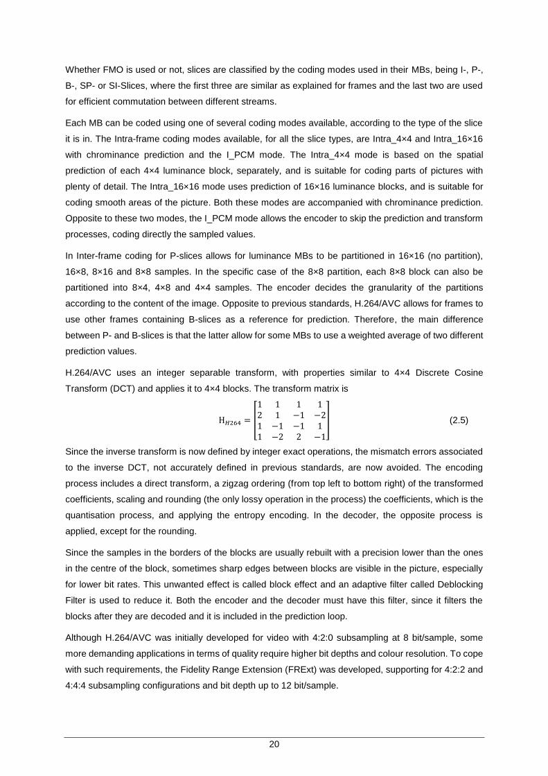
H.264/AVC uses an integer separable transform, with properties similar to 4×4 Discrete Cosine
Transform (DCT) and applies it to 4×4 blocks. The transform matrix is
H𝐻264 = [
1 1 1 12 1 −1 −21 −1 −1 11 −2 2 −1
] (2.5)
Since the inverse transform is now defined by integer exact operations, the mismatch errors associated
to the inverse DCT, not accurately defined in previous standards, are now avoided. The encoding
process includes a direct transform, a zigzag ordering (from top left to bottom right) of the transformed
coefficients, scaling and rounding (the only lossy operation in the process) the coefficients, which is the
quantisation process, and applying the entropy encoding. In the decoder, the opposite process is
applied, except for the rounding.
Since the samples in the borders of the blocks are usually rebuilt with a precision lower than the ones
in the centre of the block, sometimes sharp edges between blocks are visible in the picture, especially
for lower bit rates. This unwanted effect is called block effect and an adaptive filter called Deblocking
Filter is used to reduce it. Both the encoder and the decoder must have this filter, since it filters the
blocks after they are decoded and it is included in the prediction loop.
Although H.264/AVC was initially developed for video with 4:2:0 subsampling at 8 bit/sample, some
more demanding applications in terms of quality require higher bit depths and colour resolution. To cope
with such requirements, the Fidelity Range Extension (FRExt) was developed, supporting for 4:2:2 and
4:4:4 subsampling configurations and bit depth up to 12 bit/sample.

21
Although there are other non-standardised tools for H.264/AVC, they are under the scope of this thesis.
Different applications require different sets of tools and not all applications require all the tools that this
standard provides. Implementing all the tools in all the decoders would make most of the decoders
unnecessarily complex. Therefore, profiles and levels establish concurrence points defined in order to
allow interoperability between terminals corresponding to applications with similar functional
requirements. Initially, three profiles were defined: Baseline, Main and Extended. FRExt adds four new
profiles, all of them hierarchically built from the Main profile: High, High 10, High 4:2:2 and High 4:4:4.
According to [FaPe09], H.264/AVC has a higher compression performance, for streaming applications,
than previous standards, with average compression gains of 63% relative to MPEG-2 Video and around
37% relative to MPEG-4 Visual ASP. For videoconference applications, H.264/AVC shows a high
compression performance, around 40% better than H.263 Baseline and around 30% better than
MPEG-4 Visual SP. Also, for entertainment applications, the average compression gain relative to
MPEG-2 Video is around 45%.
The complexity and size of H.264/AVC depends on the platform it is implemented in. Therefore,
complexity is hard to assess and it is usually done based on the C code developed by JVT. Encoding
complexity of H.264/AVC is more than one order of magnitude higher than MPEG-4 Visual Simple, and
a factor of 2 higher for decoding complexity. The relation between the complexities of the encoder and
the decoder for H.264/AVC is around 10 for the simplest configurations and up to 2 orders of magnitude
for more complex configurations.
2.4 Evolved Multimedia Broadcast Multicast Service
This section briefly describes the service that within the scope of this thesis – eMBMS. This service
extends the LTE Core Network, enhancing the capability of serving many users with the same video
content at the same time and boosting the capacity for live or on-demand contents. This section is based
on [Eric13] and [Sams13].
Broadcasting the same content to many of users is a bandwidth efficient way to provide a large number
of users with the same video content, compared to a unicast transmission, where the content is
individually transmitted to each user. The main reason is that each stream requires only one data
channel in the first case, whereas in the latter each user needs a data channel dedicated to him/herself,
as represented in Figure 2.8. The consequence is that the broadcast mode can transmit a limited
number of streams to a very large number of users, whereas unicast can transmit a large number of
streams to a limited number of user. In the cases where many users are interested in having the same
content, it is advantageous to broadcast or multicast (i.e., transmit the content to a large number of
service subscribing users, but not all).

22
Figure 2.8. Broadcast versus Unicast (extracted from [Eric13]).
Since mobile communication systems are traditionally designed for unicast communication, the
coexistence of broadcast and unicast is achieved by extending the existing LTE architecture with
eMBMS-specific elements, as represented in dark blue in Figure 2.1: the Broadcast Multicast Serving
Centre (BM-SC), responsible for authentication, content authorisation, billing and configuration of the
data flow through the core network; the MBMS Gateway (MBMS-GW), whose main function is to deliver
MBMS packets to each eNB transmitting the service, using multicast; and the MBMS Coordination Entity
(MCE), responsible for allocating time and frequency resources as an MBMS scheduler that can serve
a large number of eNBs. The BM-SC adds resilience to the broadcast by using Application-Level
Forward Erasure Correction (AL-FEC) codes – which adds redundancy to the stream so that receivers
can recover packet losses – and supports the 3GPP-associated delivery procedures. These procedures
include unicast base file repair, allowing receivers to fetch the remaining parts of a file through unicast
from the BM-SC and reception reporting, so operators can collect QoE reports and make session-quality
measurements. The centralised MCE architecture allows operators to maximise the MBMS over a Single
Frequency Network (MBSFN) gains with a large MBSFN area.
In Figure 2.9, the procedures and message exchanges required for starting an eMBMS session are
represented. The BM-SC initiates the MBMS Session Start procedure when it is ready to send data, by
sending a Session Start Request to the MBMS-GW; this is a request to activate all necessary bearer
resources in the network for the transfer of eMBMS data and to notify interested and previously
registered UEs of the imminent start of the transmission. The MBMS-GW responds with a Session Start
Respond message signalling the BM-SC to send eMBMS data to the MBMS-GW after waiting for a
configurable delay that allows for the network to perform all the procedures required to enable eMBMS
data transfer. Then, the MBMS-GW stores the session attributes and allocates a transport network IP
multicast address for this session and passes the Session Start Request with the session attributes on
to the MME. The MME also stores the session attributes and passes the Session Start Request with the
session attributes on to the RAN, i.e., to the eNBs. The eNBs stores the session attributes, responds
with a Session Start Response message to the MME – which in its turn passes the message on to the
MBMS-GW after storing the eNBs identifiers – and establishes the necessary radio resources for the
transfer of MBMS data to the interested UEs. The eNB then joins the transport network IP multicast
address (including the IP address of the multicast source) allocated by the MBMS GW, to enable
reception of MBMS data. Finally, the BM-SC starts sending eMBMS data to the MBMS-GW, which sends
it using IP multicast distribution towards all joined eNBs.

23
E-UTRAN/UTRAN MBMS GW MME/SGSN BM-SC
1. Session Start Request
3. Session Start Request
6. Session Start Response
4. Session Start Request
5. Session Start Response
9. MBMS data
2. Session Start Response
UE
7. RAN Resource Setup
8. IP Multicast Join
10. MBMS data
Figure 2.9. MBMS Session Start Procedure (extracted from [3GPP11a]).
Broadcast data is sent over synchronised SFN, as illustrated in Figure 2.10, where tightly synchronised,
identical transmissions from multiple cells, using the same set of sub-frames and modulation and coding
scheme, appear to the device as a transmission from a single large cell over a time-dispersive channel,
since the several received signals are combined into a better resulting signal instead of being seen as
interference. This improves received signal quality and spectral efficiency.
Figure 2.10. SFN principles (extracted from [Eric13]).
For SFN broadcast, unlike unicast, signals arrive from many geographically separate sources and can
incur large delay spread. Consequently, one of the factors limiting MBMS capacity is self-interference
from signals reaching the receiver with a delay that is greater than the guard interval (low transmitter
density). To overcome this, a long cyclic prefix is added to MBSFN-reserved sub-frames to allow for the
time difference in the receiver.
The two main eMBMS use cases are live streaming and on-request file delivery, which enables services
such as unicast off-load (local device caching), software updates and Machine-to-Machine (M2M) file
loading. For live streaming delivery over eMBMS, MPEG Dynamic Adaptive Streaming over HTTP
(MPEG-DASH) is an option that enables high quality streaming of media content. This solution slices

24
the live stream into a sequence of media segments, which are then delivered through the system as
independent files. By using MPEG-DASH with eMBMS, the same live encoder and common clients can
be used for unicast and broadcast offerings. This solution also supports using the same system protocol
stack for both live streaming and file-delivery implementations.
Multicast, by its nature, is not a connection-oriented mechanism, so protocols such as TCP are not
appropriate. For applications such as streaming, the occasional dropped packet is not a problem, but
for distribution of critical data, a mechanism is required for requesting retransmission. The File Delivery
over Unidirectional Transport (FLUTE) protocol allows distribution of files over unidirectional links using
UDP. File delivery can also make use of the unicast file-repair feature, allowing UEs to fetch any missing
file segments. However, this feature should not be used for services with real-time requirements, such
as live streaming.
2.5 Performance Parameters
The main service relevant to this thesis is video transmission, hence, this section is focused only on the
performance parameters of LTE video services. Video quality evaluation can be classified into subjective
and objective. Subjective video quality is concerned with how video is perceived by a viewer and
designates his/her opinion on a particular video sequence. Subjective video quality tests are often
expensive in terms of time and human resources. Objective video evaluation techniques are
mathematical models that approximate results of subjective quality assessment, but are based on
criteria and metrics that can be measured objectively and automatically evaluated by an algorithm.
Objective quality models can be classified into Full-Reference (FR), Reduced-Reference (RR) and
No-Reference (NR). In the first, a detailed comparison of the input and output video stream is performed.
This is a computationally intensive process as it not only involves per-pixel processing but also time and
spatial alignment of the input and output streams. In the RR models, some reduced information about
the original video is needed, and is used along with the degraded video in order to estimate the perceived
video quality. NR models estimate the perceived video quality based exclusively in the degraded video
stream. This type of model can consider fewer factors than a FR model however can be deployed in a
much wider variety of scenarios.
The parameters that define quality in a video stream for IP video applications can be related to the video
coding process or to the network through which the video is transmitted. The first ones include
resolution, frame rate, compression. Higher resolution means that each individual picture frame is
represented by more pixels, decreasing spatial granularity. The frame rate is the number of frames
shown per second. This is a measure of time granularity, and is usually represented in frames per
second (fps). Together they strongly influence the video bitrate. Higher resolution and/or frame rate
means better video quality, but it also means higher video bit rate, and hence a higher bandwidth needed
to transmit the video. Compression techniques can be either lossless or lossy. As the name indicates,
in the former no video quality is lost, although the compression ratios are usually not satisfactory for

25
video streaming, while the latter strongly reduce the video bitrate and consequently the bandwidth
required to transmit it, but also, as the name suggests, degrade video quality.
The main network related performance parameters that have an impact on the quality of IP video
applications are packet loss and delay variation. Packet loss occurs when packets of data being
transmitted across an IP network fail to reach their destination, or are corrupted on arrival. This can
happen due to a large number of factors, such as network congestion, weak radio signals due to distance
or multi-path fading, faulty networking hardware, or faulty network drivers. When reliable delivery is
necessary, packet loss increases latency due to additional time needed for retransmission. When this
is not the case and no retransmission is performed, packets experiencing high enough delays might be
dropped, resulting in lower latency overall at the price of data loss. In terms of the impact this has on
video, it can vary from a few disruptions in the image to total frame loss. Packet delay variation is the
difference in latency between retransmitted and received packets. Even in the absence of packet loss,
packet delay variation may cause the video to freeze until a frame with higher delay arrives to the
decoder. The effects of packet delay variation in video streams can be removed by a properly sized
play-out buffer at the receiver, which may only cause a detectable delay before the start of media
playback, due to the time the buffer takes to be filled up to a minimum threshold.
2.6 State of the Art
Although this thesis is based on the H.264/AVC standard, there are other widely used coding schemes,
such as MPEG-2 Visual, H.263 or MPEG-4 Visual. The first one is popular for certain applications, such
as Digital Video Broadcast (DVB) for both standard-definition and high-definition television (SDTV and
HDTV, respectively). H.263 has a basic coding algorithm similar to MPEG-2, but with changes that make
it more efficient for coding video at low bit-rates; therefore, this standard is commonly used for
applications such as video telephony or video conference. MPEG-4 uses the same baseline H.263
algorithm, but with several additional features that improve its coding efficiency and make it suitable for
coding many types of audio-visual data. As mentioned before, video coding standards set the syntax for
the decoder and for the encoder’s output, but the encoding process itself is not standardised. This leaves
room for many coding parameters to range in order to achieve the desired balance between rate and
subjective quality for the target application.
In [WiSc03], the authors optimise encoders for the four standards mentioned above and compare their
performance by means of Peak Signal-to-Noise Ratio (PSNR) and subjective testing results. Three
separate experiments were performed, evaluating performance for video streaming, video conferencing
and entertainment-quality applications. In the first experiment, H.264/AVC showed significantly better
performance relative to the other standards, with MPEG-2 being the least adequate to this application.
For the second experiment, H.264/AVC is, again, the standard that provides the best performance with
H.263 being the worst (MPEG-2 was not tested). In the final experiment only H.264/AVC and MPEG-2
were tested and the first showed again the best performance. The authors also confirm these results

26
through sets of subjective testes, in which H.264/AVC shows even better performance relative to the
other tested standards.
As shown before, H.264/AVC allows for significant reduction of bit-rate, relative to previous standards,
for the same quality level, making it the most accepted standard for mobile TV delivery services such
as eMBMS. However, “the coding efficiency is achieved at the expense of increased traffic variability”,
[VuHu08]; the authors present a study of the transport mechanism, in order to exploit the advantages of
the standard without sacrificing spectral efficiency by performing statistical multiplexing of several video
streams. This technique “produces a combined stream, which is less bursty compared to the individual
streams”, exploiting the fact that peaks in the streams do not coincide in time. It is performed either by
coordination in between the encoders of the individual streams in order to meet the available link
capacity or by dropping P-frames when the aggregate rate of the streams exceed current channel
capacity, with the first case showing multiplexing gains in terms of PSNR and bit-rate and the latter
showing negative in most of the simulation setups. Specifically, in the case of coordinated encoding,
periodically updating the rate of the channel to meet the bit-rate requirements “do not contribute
significantly to the gains, but may reduce the PSNR variations within a stream and thus provide gains
in terms of visual quality”.
In cellular networks, two factors are important when considering video transmission: heterogeneity of
UEs and the constant changes in delivery parameters in the network. The latter manifests itself through
blocking effect, temporary playback of video stream due to buffering or even total loss of playback. In
[McDo11], the authors propose how an extension of H.264/AVC known as Scalable Video Coding (SVC)
provides a solution to the above factors. A static (no network losses) analysis of video quality when
spatial resolution (spatial scalability), number of frames per second (temporal scalability) or the
quantisation parameter (quality scalability) are ranged shows that all of these three dimensions can
cause a degradation of the quality, with spatial resolution having the most noticeable effect. As for the
analysis in an LTE network, authors verified that channel conditions and competing traffic led to packet
losses, which had different effects for the tested scalability dimensions. Moreover, temporal scalability
showed the most frequent frame loss, due to the fact that in its configuration a single layer represents
an entire I-frame, thus “when loss of a layer containing an I-frame occurs, the entire frame is lost”
whereas in the cases of spatial and quality scalability, “the I-frame data is spread across multiple layers”.
In [Sing12], the authors assess LTE capacity for stored video services, evaluate the impact of adaptive
streaming on user QoE and on the concept of Rebuffering Outage Capacity and propose a QoE-aware
RRM framework “that works in conjunction with adaptive streaming to optimise capacity under certain
QoE constraints”. Also, the authors define Rebuffering as “the state of streaming invoked when the
playback buffer is emptied in which the video playback is stalled while the buffer is being filled up”. From
here, they define Rebuffering percentage as the percentage of the total streaming time spent rebuffering.
Finally, the definition of Rebuffering Outage Capacity comes as “the number of active users that can
simultaneously stream video where users are satisfied 𝐴𝑐𝑜𝑣 percentile of the time, with a user being
counted as satisfied if and only if the rebuffering percentage in its video streaming session is less than
or equal to 𝐴𝑜𝑢𝑡. For the quality-capacity trade-off experiment, results show, as expected, that a higher

27
number of simultaneous users can be supported for lower quality streams. Also, by increasing 𝐴𝑜𝑢𝑡, the
rebuffering outage capacity increases monotonically, which is also expected – if users are content with
less, the system can support more users. If adaptive streaming is included, rebuffering outage capacity
increases very effectively, with results showing that the lowest quality adaptive stream leads to higher
capacity that the highest quality non-adaptive stream. The results with the proposed RRM show that
some perceptive quality needs to be sacrificed in order to gain from rebuffering reduction but, since user
QoE “is more sensitive to playback stall than to nominal quality degradation, the proposed technique
would lead to increase in the number of satisfied users in the system and hence translate into capacity
gains” in the range of ~20%. These results justify the adoption of H.264/AVC for the service of interest
to this thesis, eMBMS.
In [Hell11], the authors analyse the improvement in capacity introduced by layer-aware Modulation and
Coding Schemes (MCS) allocation when using SVC compared to case with single MCS and H.264/AVC
coded video transmission, based on the MBSFN channel models and MCS schemes discussed in 3GPP
Release 10. The authors start by defining four channel schemes for a MBSFN channel simulation, with
increasing modulation schemes, coding rates and, consequently, data rates. Results from simulations
show, as expected, that the high data rate channels, being more vulnerable to noise, have a lower
percentage of users receiving data with less than 1% of failure. The combination of layer-aware MCS
with SVC allows reaching the target coverage area with a significantly reduced cost in terms of allocated
channel bandwidth, by transmitting the low quality SVC base layer (SVC BL) to the whole target area
using only a portion of the available bandwidth for the robust bearer channel, whereas the remaining
bandwidth can be utilised with a less robust high data rate bearer channel to provide a high quality SVC
enhancement layer (SVC EL) to users with good reception conditions. The authors then define three
scenarios using the most robust channel scheme defined before for H.264/AVC and the SVC BL and
the remaining three channel schemes as the SVC EL, one for each scenario. An SVC BL ratio (SVC BL
data rate to the overall video data rate) of 30%, i.e., 30% of bandwidth for the SVC BL and 70% for the
SVC EL, corresponds to an increase of the capacity by more than twice compared to transmission of
H.264/AVC single-layer (SL), assuming an average SVC coding overhead of 10 %, whereas an SVC
BL ratio of 50% leads to capacity gains up to 500%. Finally, the authors define three coded video
streams – one coded as H.264/AVC SL, one as SVC 30% and one last as SVC 50% – transmitting the
same video sequences, encapsulated in RTP packets and subsequently into IP packets. As expected,
high quality SVC video is not played out flawlessly for a portion of users, whereas the SVC BL performs
as good as the H.264/AVC SL reference. The two SVC streams show similar performance but the
scenarios presented reveal that, the higher the data of the SVC EL, a higher percentage of users will
have a low playout robustness. Also, the increase in data rate of the SVC EL provokes an increase in
the percentage on users with a certain PSNR degradation. Considering the achievable capacity gain,
SVC30 clearly outperforms SVC50. Results show that there is a good trade-off between the capacity
gain and the PSNR cost, allowing for operators to find a setup that matches their needs.
In [Zhan09], the authors propose a mechanism to improve throughput in eMBMS by sacrificing
coverage, since the performance of a broadcast system “is limited by UEs in poor conditions”. An
advantage of this solution is that it allows for exact control of the coverage, by setting and adjusting the

28
threshold for the SINR of UEs, which means that it allows to control the cost of the solution. The RRM
framework used for the single-cell point-to-multipoint transmission contains a service-specific packet
scheduler that decides the TTI and the RBs in which MBMS will be scheduled; a service-specific HARQ
(Hybrid Automatic Repeat reQuest) checking the Ack/Nack feedbacks from all the UEs; and a service-
specific AMC, determining that all “subscribers must use the same MCS for a transmission”, selected
according to the worst QCI among feedbacks from all UEs. Some users in poor reception conditions
such as building insides determine the system throughput since “they are more likely to select low MCS
and request retransmissions”. Since providing coverage to such users increases the cost of delivering
the service, the authors propose that these UEs are identified and ignored by the RRM when deciding
on MCS and retransmission. For that purpose, authors define a measure determined by instantaneous
SINR as the resource cost to cover an UE. Another way of improving throughput is increasing the lowest
effective code rate, which is done by “increasing the order of the lowest MCS in candidate set and
decreasing the maximum transmission number”. The idea behind this method is very similar to the
mechanism proposed by the authors, however these parameters are discrete-value, “which means that
the adjustment of the parameters can only be performed with very coarse granularity” and cannot be
controlled. Results show that, with the threshold set to -5dB, the coverage is degraded from 99.8% to
96.5%, and the throughput gain is 22.6%. Comparing the purposed mechanism to the lowest effective
code rate alternative, the first shows much higher throughput gain, “and the coverage is even slightly
better” than the alternative. As for the Block Error Ratio (BLER), the alternative shows that although
some UEs have relative good BLER performance, they are not being covered but still they cost
resources whereas in the purposed mechanism UEs not being covered have BLER near 1, which means
that these UEs should be totally ignored by the service. “With the proposed mechanism network
operators will not only get spectral efficiency gains for MBMS but it will also enable them to adjust the
trade-off between coverage and spectral efficiency according to business requirements”.
In August 2012, at the Mobile World Congress, Ericsson (a network equipment manufacturer)
demonstrated live LTE Broadcast as the world’s first demo of end to end commercial offering of the
service, [Eric14]. In January 2014, Verizon (an American operator) announced that it would be
showcasing its LTE Multicast service, based on eMBMS, during Super Bowl week at the Verizon Power
House in New York City. In the same announcement, Verizon revealed plans to show the Super Bowl
game “to an invited audience live in the Power House over LTE Multicast”, resulting from a partnership
with network equipment manufacturer Alcatel-Lucent and device manufacturer Samsung, [Veri14].
In January 2014, [Sams14], Samsung and Korean operator KT announced the world’s first commercial
eMBMS solution to be available to KT subscribers on a specific Samsung device, starting the day after
the announcement, although the service is currently limited to selected areas of the country where it is
available. In order to access the service, with the commercial name ‘Olleh LTE Play’, subscribers must
update the software on their devices and download the operator’s mobile TV application. “In an effort to
commercialise LTE eMBMS, Samsung and KT have worked together for a number of years to develop
network equipment and device solutions”. Although Samsung plans to “actively explore partnerships
with global mobile operators to promote eMBMS solutions”, to date there are no other commercial
eMBMS service anywhere in the world.

29
Chapter 3
Models and Simulator
Description
3 Models and Simulator Description
This chapter provides a description of the models and simulators used and/or developed. First, a
description of the radio link model is given. Secondly, the video quality assessment models are
described, followed by a description of the leaky bucket model used in the developed rebuffering delay
models. Next, the OPNET Modeler simulation tool is briefly presented, followed by the simulation set up
used in this thesis and a further description of the implementation of the models used. Finally, both
simulator and models are assessed.

30
3.1 LTE Network Simulator
The LTE simulation scenarios developed in this thesis were implemented and simulated using the
OPNET Modeler, [Rive14], simulation tool. OPNET is a network simulation tool consisting of a
hierarchical modelling environment based on C/C++ programming, and has an advanced Graphical
User Interface (GUI) used for analysis and debugging. It comprises a large set of features and toolsets
including: a model library involving many protocols, a node editor for specifying network component
interface, a process editor for abstraction of behaviour of a particular network component, a project
editor for defining the topology of the network and various linkages, an open model source code editor,
and a simulation window that is able to capture and show the results of network simulation.
In the project editor, one can design a network or a simple simulation scenario using nodes and objects
from the object palette or creating new ones with the node editor. In Figure 3.1, a pre-defined eMBMS
scenario is represented where 2 eNBs is transmitting video data to 5 UEs. Actually, it is not exactly video
that is being transmitted, but random traffic generated by OPNET based on source video trace files.
These trace files contain information about the video frames of a video sequence, such as the type of
frame, the number of bits of each frame, and the order in which the frames are played out.
Each of the objects visible in Figure 3.1 has a large set of editable attributes, concerning e.g. LTE and
IP, as represented in Figure 3.2 for eNB and UE. For this thesis, the most relevant attributes are those
related to physical channels and eMBMS as shown in the figure, such as the MCS index and the path
loss parameters. For the path loss parameters, a large variety of pre-configured models are available,
such as pedestrian and vehicular, urban, suburban and rural environments and indoor propagation.
Figure 3.1. Example of a default eMBMS scenario.

31
a) eNB attributes b) UE attributes
Figure 3.2. Examples of attributes edition for two network elements of a pre-defined scenario.
After running the simulation, the results browser becomes available, where one can choose from a large
variety of simulation results to be shown, as depicted in Figure 3.3. These results can be object-specific
statistics (e.g. for a specific UE or eNB) or network global statistics. Either global or object, the results
can be shown separately in dedicated windows or by combining several results to be grouped and
shown in the same window. In Figure 3.4, the values for the received throughput over the simulation
time, for a specific UE from the scenario of Figure 3.1, are represented. The data from these graphs can
be exported to a spreadsheet for more extensive analysis, and can be refreshed after another simulation
run (avoiding the need to select the wanted results at each simulation run).
Figure 3.3. Example of available results from the OPNET simulation Results Browser.
Although it is a powerful network simulation tool, OPNET is not designed for video transmission, does
not provide any video-specific performance metric, and does not allow for actual video to be transmitted

32
between nodes. Also, OPNET is not pre-configured to write a trace file of the received packets at the
UEs at the end of each simulation run; a configuration of this functionality would require the edition the
UE node module in the simulator, which goes beyond the scope of this thesis. Therefore, the
assessment of video quality can only be done relying on simple NR models described in Section 3.3,
using the available metrics, such as those shown in Figure 3.3.
Figure 3.4. Example of network simulation results, in this case showing the received throughput over
the simulation time for a specific UE in several simulation runs.
3.2 Radio Link Model
This section provides a brief description of the LTE physical layer implementation in OPNET, [Rive13].
An eNB can deploy a physical profile either supporting FDD or TDD. Some frame structure and
frequency domain parameters, such as frame length or RB allocation, are fixed and implemented as
defined in Section 2.1.2. Duplexing scheme, bandwidth, base frequency and CP length are also
implemented as described in that section, but these are configurable. The PBCH, PDSCH, PDCCH,
PUSCH and PUCCH physical channels are also modelled as described in the same section.
Physical layer measurements of SINR are supported for both PUSCH and PDSCH. A measurement
entity is created for each UE, which records instantaneous values of SINR and smoothes them by using
a measurement window; thus, the measurement module computes a moving average and the size of
the measurement window can be configured. For DL, separate measurements are collected for each
sub-band of the channel if the scheduler is expected to use Channel Dependent Scheduling, or no
measurements are collected at all, depending on the efficiency mode. Physical layer measurements of
Reference Signal Received Power (RSRP) and Reference Signal Received Quality (RSRQ) are
supported. A measurement entity for RSRP and another for RSRQ is created for each audible eNB,

33
thus the UE continuously measures RSRP and RSRQ for all eNBs within range in the operating
frequency. Reference signals are not transmitted or received in the model, therefore RSRP and RSRQ
measurements are performed on the primary and secondary synchronisation signals. Thus, the physical
layer updates RSRP and RSRQ every 5 ms. The physical layer also sends indications to the higher
layers if the measured RSRQ (averaged over 200 ms) violates configured thresholds.
The maximum power is a configurable parameter at both eNBs and UEs, and is the transmission power
of the device over the entire channel bandwidth. Actual burst transmissions use a transmission power
proportional to its assigned portion of the bandwidth. The antenna gains at both eNB and UE are
configurable either via an attribute or by using an antenna mode. For eNBs with multiple sectors, only
the antenna model can be used, as it describes the directionality of the antenna on each of the sectors.
The ITU Multipath Channel models Pedestrian A, Pedestrian B, Vehicular A and Vehicular B, [3GPP02],
are supported, but more can be added. The multipath fading channel consists of a finite state Markov
chain (FSMC) that captures the time evolution of the multipath channel and channel state dependent
effective SNR mapping functions; these functions are used to compute the effective SNR for a given
channel state. The next state transition of the FSMC is governed by a transition probability matrix (TPM);
the TPM and the channel state dependent effective SNR mapping functions together define the
behaviour of a multipath channel model. The path loss model is selected from the following, among
several models available:
Free space
3GPP-based model - Urban microcell
ITU-R M.2135-based models
o Urban Micro (UMi)
o Rural Macro (RMa)
The 3GPP Urban microcell and the ITU-R M.2135-based models used in this thesis are described in
Annex B and Annex C, respectively. Although some of the presented models have configurable
parameters, most of them are fixed. Shadow fading is also supported as the log-normal distribution.
The interference model is supported as follows. The module detects time and frequency overlaps among
different bursts. Interference, proportional to the amount of burst overlap, may cause burst drops for
PUSCH and PDSCH bursts and its effects for control channels, i.e., errors in the transmission of control
signals, are based on a uniform distribution function.
The MCS Index is configurable on UE nodes and remains fixed during the entire simulation. This
attribute does not affect the simulation when Link Adaptation is activated. In this case, the MCS index
is dynamically changed based on the link adaptation procedure. Modulation curves plotting the SNR
versus BLER are available for all MCS indices. Convolutional turbo coding with circular rate matching
algorithm are implemented in obtaining the modulation curves.
Both SISO and MIMO models are supported. The latter can be used either for antenna diversity or for
spatial multiplexing, as described in Section 2.1.2. By default, the eNB supports two transmit antennas
and two receive ones, and the UE supports one transmit antenna and two receive ones.

34
3.3 Video Quality Assessment Models
In this section, the video quality assessment models used in this thesis are described. Due to the
previously mentioned simulator limitations, only NR models can be applied in this work. The first of these
models is proposed in ITU-T Recommendation G.1070 [ITUT07] as a QoE planning tool for point-to-
point videophone applications over IP networks. The model incorporates network, application and
terminal quality parameters of high importance for QoE planning and, opposite to previous
recommendations, calculation of video quality is now done without the need of using a video signal,
which is a key feature for this work as mentioned before. The input parameters used in the model are:
Video codec specifications and codec implementation;
Spatial resolution – theoretical spatial resolution employed in a codec;
Video display size – the size of the UE display where video is being played;
Key frame interval – the time interval in which the video is coded solely from intra-frame
information;
Video packet loss ratio, 𝑃𝑝𝑙 [%], referring to end-to-end IP packet loss ratio;
Video frame rate, 𝐹𝑟 [fps], used in the encoder;
Video bit rate, 𝐵𝑟 [kbps], at the encoder.
The video packet loss ratio parameter is obtained from OPNET. The remaining parameters are encoding
parameters and are characteristic of the video sequence.
The output of this model is an estimation of subjective video quality, 𝑉𝑞 in the form of an estimated Mean
Opinion Score (MOS) – an arithmetic mean of the scores attributed by different individuals, which can
range from 1 (worst) to 5 (best), [ITUT08].
The estimation for subjective video quality is calculated as:
𝑉𝑞 = 1 + 𝐼𝑝𝐼𝑐 (3.1)
where 𝐼𝑝 is a representation of the video quality degradation introduced by the packet losses in the
transmission process, and can be expressed as:
𝐼𝑝 = exp {−𝑃𝑝𝑙
𝐷𝑃𝑝𝑙
} (3.2)
where 𝐷𝑃𝑝𝑙 is the packet loss robustness factor and represents the degree of video quality robustness
due to packet loss.
In (3.1), 𝐼𝑐 is a representation for the basic video quality affected by the coding distortion under a
combination of 𝐹𝑟 and 𝐵𝑟, and can be expressed as:
𝐼𝑐 = 𝐼𝑂𝑓𝑟 exp {−(ln 𝐹𝑟 − ln 𝑂𝑓𝑟)
2
2 𝐷𝐹𝑟2 } (3.3)
where:
𝐷𝐹𝑟 is the degree of video quality robustness due to frame rate 𝐹𝑟;

35
𝑂𝑓𝑟 an optimal frame rate that maximises the video quality at each video bit rate 𝐵𝑟 and is
expressed as:
𝑂𝑓𝑟 = 𝑣1 + 𝑣2𝐵𝑟 (3.4)
If the video frame rate is the optimum that maximises video quality, 𝐹𝑟 = 𝑂𝑓𝑟, then 𝐼𝑐 = 𝐼𝑂𝑓𝑟, where 𝐼𝑂𝑓𝑟
represents the maximum video quality at a video bit rate 𝐵𝑟 and is expressed as:
𝐼𝑂𝑓𝑟 = 𝑣3 +
𝑣3
1 + (𝐵𝑟
𝑣4)
𝑣5
(3.5)
The degree of video quality robustness due to frame rate 𝐹𝑟 is expressed as:
𝐷𝐹𝑟 = 𝑣6 + 𝑣7𝐵𝑟 (3.6)
The packet loss robustness factor is expressed as:
𝐷𝑃𝑝𝑙= 𝑣10 + 𝑣11 exp {−
𝐹𝑟
𝑣8
} + 𝑣12 exp {−𝐵𝑟
𝑣9
} (3.7)
Coefficients 𝑣1, 𝑣2, …, and 𝑣12 are dependent on the first four input parameters listed above and can be
found in Table D.2.
In [JoSo14], the authors tested the G.1070 model in a Terrestrial DTV scenario, obtaining a Pearson
Correlation (PC) between the actual 𝐼𝑝 values, derived from subjective tests, and the values obtained
from (3.2) of 0.60 and a Root Mean Square Error (RMSE) of 0.30 (in a 0-1 scale), which are not good
results, concluding that the impact of a particular loss has a great variance depending on the impacted
slice (I, P, or B). As stated in Section 2.3, since B and P slices depend on information from I ones, the
loss of I slices affects much more than P or B ones, and, analogously, the loss of P slices affects more
than B ones. With these considerations, the authors propose a new metric representing the weighted
percentage of slice loss, 𝑝𝑤, which can be expressed as:
𝑝𝑤 = 𝑥1𝑃𝑝𝑙𝐼+ 𝑥2𝑃𝑝𝑙 𝑃
+ 𝑃𝑝𝑙𝐵 (3.8)
where:
𝑃𝑝𝑙𝐼, 𝑃𝑝𝑙𝑃
and 𝑃𝑝𝑙𝐵 are the packet loss ratios in I, P and B frames, respectively;
𝑥1 and 𝑥2 are two coefficients, representing the average number of affected slices when there
is an error in an I or in a P slice, respectively.
Also, the authors have found that 𝐼𝑝 can be correlated with 𝑝𝑤, selecting the appropriate values for 𝑥1
and 𝑥2, as:
𝐼𝑝 =1
1 + 𝑘𝑝𝑤
(3.9)
where 𝑘 is a constant. The values of 𝑥1, 𝑥2 and 𝑘 that minimise the RMSE between the actual 𝐼𝑝 values,
derived from subjective tests, and the values obtained from (3.9) are presented in Table 3.1. With these
values, the obtained PC is 0.84 and the RMSE between the actual and the derived 𝐼𝑝 values is 0.16,
these values being much better than those obtained by using the G.1070 model.

36
Table 3.1. Optimal values for 𝑥1, 𝑥2 and 𝑘 (extracted from [JoSo14])
𝑥1 21.5
𝑥2 5.7
𝑘 26.9
The authors also recommend that, for a better correlation between subjective and derived values of 𝑉𝑞,
𝐼𝑐 should be calculated using the expression in [JoAr11]. Since the expression in cause contains a
coefficient depending on video content and since in this thesis a generic model not depending on video
content is needed, 𝐼𝑐 is calculated using the expression from model G.1070 in (3.3).
3.4 Leaky Bucket Model
One of the parameters that affect QoS of a video broadcast service is the probability of occurrence of
rebuffering events which, as mentioned before, occur when the decoder buffer is emptied and it
provokes the video playback to stall. As this metric strongly depends on the size of the decoder buffer,
the buffer size should be designed so that the decoder can decode the video bit stream without suffering
from buffer overflow or underflow. This implies that the choice of the buffer size must be made
considering the typical peak bit rate of the applications for which the decoder is designed. For this goal,
the authors in [RiCh03] propose a hypothetical reference decoder (HRD) based on an idealised decoder
model that decoder manufacturers can use as a reference for their implementations. The buffer size for
this HRD is determined using a leaky bucket model which, as the name suggests, is based on an
analogy of a bucket that has a hole in the bottom through which any water it contains will leak away at
a constant rate, until or unless it is empty. Water can be added intermittently, i.e., in bursts, but if too
much is added at once, or it is added at too high an average rate, the water will exceed the capacity of
the bucket, which will overflow. In this analogy the bucket represents the decoder buffer and water
represents bits of information being added to and decoded out of the buffer. This analogy also suggests
that the leaky bucket model is designed for CBR channels, but it can also be used with VBR channels.
The VBR case will be considered, since both the video trace file used in this work was coded with VBR
and the radio channel is a VBR one. For these channels, having a sustainable peak bit rate 𝑅′ greater
than the long-term average bit rate 𝑅 of the encoded video sequence, it is beneficial to characterise the
encoded sequence using a leaky bucket with the higher leak 𝑅′ rate at the encoder, yet allowing the
leaky bucket to underflow when the channel drains the bucket faster than the encoder can fill it. To
illustrate, Figure 3.5 shows the encoding and decoding schedules using a leaky bucket with the higher
leak rate. The later/lower bound on the encoding schedule is the schedule by which bits drain from the
encoder leaky bucket and are transmitted or packetised. In the figure, flat spots in this transmission
schedule indicate intervals in which the bucket is empty because there is nothing to transmit.

37
Figure 3.5. Leaky bucket bounds in the VBR case (extracted from [RiCh03]).
The earlier/upper bound on the encoding schedule represents the capacity constraint of the leaky
bucket: an upward shift of the transmission schedule by 𝐵′ bits. Since the bucket drains at a rate 𝑅′
greater than 𝑅, the bucket can have a capacity 𝐵′ smaller than 𝐵, while still not overflowing, and can
start with an initial state 𝐹′ smaller than 𝐹, where 𝐵 and 𝐹 are the buffer size and initial state,
respectively, for the CBR case. The transmitted bits enter the decoder buffer after a constant
transmission delay δ. If, after the first bit enters the decoder buffer, the decoder delays at least
𝐷′ =𝐹′
𝑅′ (3.10)
seconds before decoding the first frame, then the decoding schedule is guaranteed not to underflow the
decoder buffer. Furthermore, with delay 𝐷′, if the capacity of the decoder buffer is at least 𝐵′, then the
decoding schedule is guaranteed not to overflow the decoder buffer. In either the CBR and VBR case a
single leaky bucket is specifiable by three parameters (𝑅, 𝐵, 𝐹), where:
𝑅 is the peak transmission bit rate (in bits per second) at which bits may leave the encoder
buffer and enter the decoder buffer after a constant delay;
𝐵 is the capacity (in bits) of the encoder or decoder buffer;
𝐹 is the initial decoder buffer fullness (in bits) before the decoder can start removing bits from
its buffer. 𝐹 and 𝑅 determine the initial or start-up delay 𝐷, according to (3.10).
Further description on how to obtain the buffer size 𝐵 for a given peak transmission bit rate 𝑅 is provided
in [RiCh03]. Also, the code for a Matlab program that computes the 𝐵(𝑅) curve for a given bit stream is
provided. The curve in Figure 3.8 was obtained using an adaptation of the provided program for the bit
stream corresponding to the video trace set as input of the simulator in this work, as described further.
3.5 Global Model Simulator
The global simulator is composed of two modules, Figure 3.6: one corresponding to OPNET, previously
described, and another in C program, developed by the author of this thesis. The latter is described in

38
this section, as well as their inputs and outputs and the various stages of the simulation process.
Figure 3.6. Simulation overview and input/output files (module developed by the author of this thesis
highlighted in blue).
3.5.1 Simulator set up
The setup for the base scenario, described further, is represented in Figure 3.7. As most modules remain
unchanged for all scenarios, other will have their attributes and/or positions configured according to the
scenario parameters. The Applications module defines the applications supported by the UE nodes,
such as video streaming. The LTE Configuration module defines the LTE physical layer parameters,
such as bandwidth, base frequency or MBMS areas. The Profiles module defines user activity profiles
representing several usage patterns, including the applications used in each profile. As the EPC node
as a limit of 8 ports, and one of them is used for connecting the EPC to the IP Cloud, in scenarios with
more than 7 eNBs more than one EPC are used, according to the number of eNBs in the scenario. The
Multicast Source (mcast_src) node represents a workstation with client-server applications running over
TCP/IP and UDP/IP, which defines the multicast addresses and the applications to provide each
address. The radio propagation model is defined for each user in the respective node. eNBs are
assumed not to be sectorised, since that is how eNBs are pre-configured in OPNET. In the scenario
represented in Figure 3.7, the UE_1 node is expected to move from one of the represented eNBs to the
other. Besides that, the node is represented in a position far from the point where it was supposed to
start moving. This is due to the fact that the multicast service requires a configuration start-up delay of
approximately 110 s, Figure 3.4, but the user starts moving immediately as the simulation begins.
Hence, the initial distance between UE_1 to eNodeB_1 is the distance covered by the UE in the first
110 s of simulation.
As the number of lost packets and the packet loss ratio are not measured by the simulator, and in order
to calculate the packet loss ratio, the total number of packets per second that are supposed to arrive the
UEs, considering no packet loss, needs to be obtained. This is achieved by inserting an extra UE next
to the one of the eNBs, with free space propagation, so that this UE receives all the packets with no
losses and it will serve as reference for the calculation of the packet loss ratio of other UEs. This
reference UE is represented in Figure 3.7 as UE_0, positioned 20 m away from eNodeB_1.

39
Figure 3.7. Simulator set up for Model Assessment.
Despite the mentioned limitations of the simulator regarding video, it allows for a Comma-Separated
Values (CSV) file containing the sizes, in bytes, of each frame of a video sequence, to be input; then, it
generates traffic according to the input file. This CSV file can be obtained from a video frame trace file,
which in its turn is obtained from encoding of a video sequence. A video trace file contains the sizes of
each individual encoded video frame, in bits, frame types, the time at which each frame should be
played, in milliseconds, and frame qualities. As the simulator only needs the information about the frame
sizes, it must be extracted from all the information contained in the trace file and converted from bits to
bytes. The simulator will then generate random traffic based on the video frame sizes, i.e., with the same
bit rate as the video, getting as close as possible to actually transmitting video. The definition of the
applications and their attributes, such as the video trace file in the case of this thesis, are defined in the
Applications module represented in Figure 3.7. The used video frame trace file was extracted from
[ASU14], being generated from the encoding of an excerpt of the film Terminator 2: Judgement Day and
the acquisition, the usage of this trace file being described in [SeRe04]. The parameters describing the
trace file are summarised in Table 3.2. Although the trace file was obtained from a 600 s video sequence,
in most of the simulations only the first 100 s were used. This means that the values for the mean and
peak frame bit rates in the simulations are not the ones represented in the table, but 1.516 Mbps for the
mean bit rate and 2.188 Mbps for the peak bit rate.
Table 3.2. Video trace files parameters (extracted from [ASU14]).
Parameter Default values
Encoder H.264 FRExt
Encoding type VBR
Frame Size HD 1280×720 pixels
Frame Rate (fps) 30
GoP Size 12
Number of B frames 2
Quantiser 28
Mean Frame Bit Rate (Mbps) 2.214
Peak Frame Bit Rate (Mbps) 21.72

40
The number of simulation runs desired and their respective initialisation seeds are set on the simulator
and the simulation runs are executed in series or in parallel, depending on the number of cores of the
machine running them.
After the simulation is completed, the simulator results browser is opened, allowing for statistic results
to be shown in one single or multiple plots. As explained before, the relevant statistic is the throughput,
in packets per second, received at each UE, including the reference UE. Also, in order to apply the
adaptation of the video quality estimation model proposed in [JoSo14], the throughput, in bits per
second, received at the reference UE is also needed in order to determine the packet loss rate for each
frame type. These statistics are shown in a single graph, containing the results for all simulation runs,
and data are then exported to an XLS spreadsheet file, Lost_packets_statistics.xls in Figure 3.6.
3.5.2 Video Quality Models
After simulations are run, the packet statistics need to be converted into a video quality metric, i.e.,
MOS. This is done by applying the models described in Section 3.3 through a module developed in C,
represented in Figure 3.6 as Video Quality Assessment Model. The inputs of this module are the XLS
file containing the throughput statistics per second, for all UEs and all simulation runs, and the video
frame trace file used to determine the traffic profile in the simulator.
The video quality model module starts by reading the video trace file and storing the data about time,
type and number of bits of the video frames. Next, it reads the other input file – the packet statistics XLS
file for the current scenario and calculates the number of bits per packet at each simulation second, by
dividing the throughput of the reference UE, in bits per second, by its throughput in packets per second.
Afterwards, the global (regarding frame type) packet loss ratio is calculated for each UE and for each
simulation run, by dividing the throughput of the UE by the throughput of the reference UE, both in
packets per second. This is the metric to be used in the original G.1070 model. For the model proposed
in [JoSo14], from this point on referred to as JoSo model, an estimation of the packet loss rate of each
frame type is required and it is the next and longer step of the process. This step is repeated for each
second of simulation and starts with summing the total number of bits of each frame type in the current
simulation second, as stated in the trace file. Then, the number of packets containing each frame type
in that second is obtained by dividing the total number of bits of that frame type by the number of bits
per packet, obtained before. Afterwards, the percentages of packets that contain frames of each frame
type are computed by dividing the number of packets containing each frame type by the total number of
packets. These percentages will be used as the probabilities of a lost packet contain each of the frame
types. After determining the total number of lost packets, by subtracting the number of packets received
by the reference UE with the number of packets received by the current UE, for each lost packet, it is
randomly determined from which frame type was the data it was containing, taking in consideration the
obtained probabilities. After repeating this for all the lost packets, it is now obtained the number of lost
packets containing information from each frame type. With these values, it is now possible to calculate
the packet loss ratio of each frame type, needed for the JoSo model. Afterwards, the estimation of MOS
according to the two models described before is obtained applying the equations in Section 3.3.

41
As described in Section 3.3, the equations describing the G.1070 video quality estimation model contain
12 coefficients that depend on coding and UE parameters. The model originally provides 5 sets of
coefficients obtained for different parameters. Initially, the coefficient set #5 was chosen, since these
are the only coefficients obtained for an H.264 codec. However, in initial tests, it seemed impossible do
obtain MOS estimations of 1 or 5, even in total or absence of packet loss, respectively. This was due to
the term representing coding distortion in (3.1). As the trace file was obtained from a VBR-coded video
sequence, the video bitrate deviations from the mean value strongly affected this term and,
consequently, the quality estimation. In order to avoid this influence of VBR coding, a new set of
coefficients was determined, as described in Annex D, being represented in Table D.2 as coefficient set
#5’, as it was based on the original #5 set.
Finally, the module ends by writing both MOS estimations at each second, for each user and each
simulation run in one XLS file for each simulated scenario, represented in Figure 3.6 as
Final_Results.xls. This results file is created with the .XLS extension in order to be read with Microsoft
Excel, a tool that makes it easy to analyse large amounts of data such as the video quality estimation
for each second of simulation, for each user and for each simulation run.
3.5.3 Rebuffering Delay Models
As they make use of the same parameters as the video quality estimation models, the two rebuffering
delay models described in this section were developed and included in the same C program as the
models described in the previous section. These two models were developed by the author of this thesis
and for both of them the decoder buffer size is needed and is computed using the Leaky Bucket Model
presented in Section 3.4. As stated there, the authors of the article on which that section is based
provided the code for a Matlab program that computes the minimum buffer size for a certain peak bit
rate. In order to make it simpler to apply the rebuffering models, this Matlab code was adapted and
implemented in C, so that the Leaky Bucket Model could be integrated in the global Models program.
By applying the Leaky Bucket Model with the video trace file presented in Section 3.5.1, the plot of leaky
bucket parameters (𝑅, 𝐵), represented in Figure 3.8, was obtained.
Figure 3.8. Illustration of peak bit rate 𝑅 and buffer size 𝐵 values for the test bit stream.
Although the model was used with peak bit rates ranging from 50 to 3 000 kbps in increments of 50 kbps,
as defined in the original code, only the values starting in 1 800 kbps are represented in order to make
0
2
4
6
8
10
1800 2000 2200 2400 2600 2800 3000
Bm
in [kbit]
Thousands
R [kbps]

42
the plot legible in the zone of interest; this zone is around 2 200 kbps, since, as mentioned in Section
3.5.1, the peak bit rate 𝑅 used in the simulations is 2.188 Mbps. The corresponding buffer size 𝐵 was
obtained using linear interpolation between the 2 150 and 2 200 kbps points:
𝐵 = 𝐵1 +𝐵2 − 𝐵1
𝑅2 − 𝑅1
(𝑅 − 𝑅1) (3.11)
where:
(𝑅1, 𝐵1) is the point in the lucky bucket plot corresponding to 2 150 kbps;
(𝑅2, 𝐵2) is the point in the lucky bucket plot corresponding to 2 200 kbps.
The resulting buffer size is 2 183 kbits (approximately 273 kB), being the value used in the two
rebuffering delay models presented next.
The first of the rebuffering delay models to be developed was based on the fact that a buffer with size
𝐵 bits, considered to be initially full, being leaked at an average rate of 𝑅 bits per second but not being
filled, takes an average 𝐷 seconds to be completely emptied:
𝐷 =𝐵
𝑅 (3.12)
Considering the buffer size obtained above and the average bit rate of 2.156 Mbps mentioned in
Section 3.5.1, the maximum rebuffering delay allowed for the tested video sequence is 1.44 s, which is
rounded up to 2 s, because the sampling rate of the results statistics is set to 1 sample per second in
OPNET. This means that, if a UE is 2 s consecutively without receiving any data, the buffer will be
emptied and the video will stall. As a matter of fact, the UE does not need to stop receiving packets for
2 s to make the video to stall. As defined in Table 4.12, a MOS of 1 means no service, i.e., no video is
being played, which is equivalent to say that the video is stalled. From the video quality estimation
models described in the previous section, it was observed that such score is achieved when the packet
loss ratio is above approximately 28%. This means that, if more than 28% of the information is lost, the
decoder cannot decode the frames and no frame is displayed, hence, the model basic idea was
reformulated: if a UE receives data with a packet loss ratio higher than 28% for 2 s consecutively, the
video will stall. Applying the model to several UEs, it gives an estimation of the percentage of satisfied
users, where a user is considered to be satisfied if the video never stalls during a simulation run. Another
viewpoint is that, by applying the model to a single UE for several simulation runs, it gives the probability
of that user being satisfied. This model is referred to as Max Delay model from this point on. In the C
program, this model simply reads the global packet loss ratio statistics computed before and searches
for 2 consecutive values above 28%. This search is done for each UE and for each simulation run.
Since this is a very simplistic way of measuring the occurrence of rebuffering events, a more accurate
model was developed, trying to approximate what actually happens in a decoder buffer, therefore
referred to as Realistic model. In the decoder buffer, bits are inserted at the rate at which they are
received in the UE. After the buffer reaches a certain initial fullness 𝐹, as described in Section 3.4, bits
start being removed from the buffer at the rate at which they are decoded. In the C program, the buffer
is simply represented by a variable indicating the number of bits in it. As the received packet statistics
are read, the buffer fullness is increased by the number of bits received. When the buffer reaches its

43
initial fullness, defined here as 50% of the buffer capacity, the program starts reading the trace file and
removing bits from the buffer, i.e., decreasing the buffer fullness variable, at the rate indicated by the
trace file. If the buffer fullness reaches 0, the video stalls and the decoder starts rebuffering. When
removing bits from the buffer to be hypothetically decoded into a frame, the program does not know
whether all the bits describing that frame where received or not at the UE, and it decreases the buffer
fullness as if the bits were all available. This implies that even few packet losses (i.e., a number of bits
equal to the buffer capacity being lost) during the entire simulation would cause the buffer to become
empty, which is not realistic at all. As the Max Delay model, this one also required some adjustments.
This was done by considering that, according to the packet loss ratio in each second, the UE either
receives the total information it was supposed to, or it receives none. In other words, if the packet loss
ratio in a second is low enough, it is considered that no losses occurred during that second and all the
bits were received. On the other hand, if the packet loss ratio is high enough, it is considered that no
packet was received and no bits are added to the buffer. As explained in the Max Delay model, it is
observed that in order for a service to be provided (with higher or lower quality) the packet loss ratio is
required to be under 28%. Again, this was the value chosen for the packet loss ratio threshold. As in the
Max Delay model, the purpose of this model is to estimate the percentage of satisfied users, i.e., users
that never experiment rebuffering events, or the probability of a user being satisfied. Although this model
is more accurate than the Delay model, it is still not very realistic, as rebuffering events might be
provoked by events of total packet loss scattered over the whole simulation time and it is not supposed
to happen.
3.6 Models and Simulator Assessment
In order to assure that the simulator and the models are properly configured and implemented, both the
simulator and the models had to be assessed, so that the validity of the simulation results can be
guaranteed. First, the minimum number of simulation runs that assures statistical relevance needs to
be determined. This was obtained by simulating 100 times the same base scenario, consisting of an 2
eNBs separated by 800 m and 1 eNB stopped at ¼ of the way between the eNBs (i.e., 200 m away from
one of them and 600 m away from the other), during 100 s for each simulation run. The DL base
frequency was 1 805 MHz, therefore the propagation model was the COST 231 Walfisch-Ikegami one,
presented in Annex B. An MCS index of 21 was used, which, according to Table 4.13, corresponds to a
64-QAM modulation. After applying the video quality model to the simulation results, the next step is to
calculate the average and standard deviation of the results from first n simulation runs, for n between 1
and 100, as represented in Figure 3.9.
The average and standard deviation for the results were calculated using (3.13) and (3.14), respectively.
µ =1
𝑁𝐴
∑ 𝐴𝑖
𝑁𝐴
𝑖=1
(3.13)

44
where:
𝑁𝐴 is the size of the population;
𝐴𝑖 is the value of the i-th element.
𝜎 = √1
𝑁𝐴
∑(𝐴𝑖 − µ)2
𝑁𝐴
𝑖=1
(3.14)
Figure 3.9. Average and standard deviations of the MOS at the UE for varying number of simulations.
From Figure 3.9, one can observe that both average and standard deviation values for both models
show some oscillations when a low number of simulation runs is considered and, as the number of
simulation runs is increased, the values become stable. Thus, the minimum number of simulation runs
that assures statistical relevance is chosen as the value at which the lines oscillation stops or becomes
as low as wanted. It was considered that from 20 simulation runs on the values become approximately
constant and, therefore, this value was chosen as number of simulation runs for each scenario.
The real time duration of a simulation run is strongly influenced by the number of UEs and eNBs
considered, the simulated time, the MCS index, the average bitrate of the video sequence being
transmitted, and also on the specifications of the machine running the simulator. Other simulation
parameters have less significant impact on the simulation duration. For the scenario used in this
assessment, described above, and the simulator running on a 2.2 GHz Intel Core i7 with 6 GB RAM
laptop, the average simulation time goes up to approximately 25 s. Although OPNET allows for
simulation runs to be runt in parallel over the several cores of the machine, it requires a licence for each
core, and only one licence was available. Considering 20 simulation runs, the total simulation duration
for each scenario goes up to approximately 9 minutes.
Regarding the assessment of the simulator, the video quality models and the delay models, one test
case was simulated for each. Starting with the video quality estimation models presented in Section 3.3,
the test scenario used was similar to the one used to assess the number of simulation runs. In this test,
the objective is to estimate the video quality perceived by a user depending on its position between the
2 eNBs. Instead of testing with a stopped user, varying its position at each simulation, it was chosen to
simulate a user moving between the eNBs at pedestrian speed, so that the effects of mobility in the
perceived quality were as low as possible. If the eNBs are enough apart from each other, a decrease in
the perceived quality is expected at some point next to the half way between the eNBs. In order for this
0
1
2
3
4
5
0 10 20 30 40 50 60 70 80 90 100
MO
S
Simulation Runs
<MOS G.1070>
<MOS JoSo>
σ(MOS G.1070)
σ(MOS JoSo)

45
decrease in quality to be well noticed, the distance between the eNBs was chosen to be 800 m.
Considering this and selecting a pedestrian speed of 1.6 m/s, the total time that the user takes to move
from one eNB to the other is exactly 500 s, hence being chosen as the simulation duration for each
simulation run in this test. The variation of the quality estimation with the distance from the user to the
first eNB, for both video quality estimation models, is represented in Figure 3.10.a). As expected, the
MOS estimation is close to 5 in the surroundings of each eNB (for approximately 100 m) and then, as
the user moves away, the MOS estimation decreases until the user reaches the half distance between
eNBs. This suggests that the models are accurate and well implemented.
a) eNBs 800 m apart b) eNBs 1000 m apart
Figure 3.10. Influence of the distance between eNBs in the MOS.
Another interesting aspect to test is what happens if the distance between the eNBs is increased to
1 000 m. In order to keep the effect of mobility consistent with the previous test, the UE speed was not
changed. This means that the user now takes 625 s to move from one eNB to the other, which is the
simulation duration for this test. It is expected that the mentioned quality decrease in the half way zone
is both larger and deeper than previously. These results are confirmed as shown in Figure 3.10.b).
Comparing both figures, one can observe that the estimated MOS is close to 3 at the half way point in
the first figure and close to 2 in the second. This is expected, since in the latter case the user is at a
larger distance from any eNB than in the first case. Another aspect that one can take from this
assessment is that the video quality models show high correlation with each other, as can be seen in
both figures. Consequently, in further results analysis only the JoSo model is considered.
Next, the assessment of the rebuffering delay models was made using the same scenario, but now
considering a user stopped at varying positions, for 100 s in each one, because these models measure
the occurrence of rebuffering events during the whole simulation time and, if the user is moving it
occupies several positions in the same simulation. This would make it impossible for one to establish a
relation between the position of the user and the probability of the user being satisfied with the service,
i.e., the probability of not occurring any rebuffering event during the simulation. For this assessment,
MOS is ignored and user satisfaction is based solely on rebuffering occurrence probability. Initially,
simulations were made varying the position of the user in 50 m between each simulation, but in the end
it became clear that, in the half way zone, a higher detail was needed, since this was verified as the
zone were the rebuffering probability stops being 0%. Therefore, in the 400-600 m zone, simulations
1
2
3
4
5
0 200 400 600 800
MO
S
Distance [m]
<MOS G.1070>
<MOS JoSo>1
2
3
4
5
0 200 400 600 800 1000
MO
S
Distance [m]
<MOS G.1070>
<MOS JoSo>

46
were made for each 25 m. The models results are shown in Figure 3.11.
Figure 3.11. Probability of user satisfaction according to distance to 1st eNB as an assessment of the
delay models.
As expected, in the surroundings of both eNBs (approximately 300 m), the probability of the user being
satisfied with the service is 100% since, as seen in the assessment of the video quality model, the
packet losses in these zones are none or not enough to create emptiness of the decoding buffer. In the
300-700 m zone, the packet loss ratio becomes higher, and buffer emptiness may occur, leading the
playback to stall. Obviously, this effect is more significant the larger the distance from the user to any of
the eNBs is. This test suggests that these models are well designed and implemented. As for the video
quality estimation, the rebuffering delay models also show a very high correlation with each other.
Finally, the simulator itself was assessed. For this assessment, since OPNET is a commercial product
and none of its modules or components were neither developed nor modified in this thesis, extensive
tests to it are redundant. Instead, a single scenario was tested in order to assure that the MBMS scenario
is well configured and the MBSNF is working properly. For this, the same scenario used to assess the
quality estimation models was tested, but this time MBSFN was turned off in both eNBs. The results
from this test were then compared with the quality estimation values according to the JoSo model from
Figure 3.10.a). The expected results are that the quality estimation without MBSFN is much lower than
the results with MBSFN, since in the first case interference is constructive and in the latter it is
destructive. Since both tests were made with only 1 UE, scalability of number of users due to delivery
synchronisation of MBMS is not visible here. The results of this test are represented in Figure 3.12.
Figure 3.12. Influence of constructive or destructive interference resulting from MBSFN being enabled
or disabled, respectively.
0%
20%
40%
60%
80%
100%
0 100 200 300 400 500 600 700 800 900 1000
Satisfied U
sers
Distance [m]
Realistic model
Max Delay model
1
2
3
4
5
0 200 400 600 800
MO
S
Distance [m]
<MOS JoSo> MBSFN on<MOS JoSo> MBSFN off

47
As expected, the estimated quality in the case of MBSFN turned off is much lower than the case with
MBSFN turned on, in the entire simulation. In the first case, the user can only receive an acceptable
service in a 50 radius next to an eNB, whereas in the latter the service is acceptable in a 250 m radius,
where acceptability of service is defined here as having a MOS above 4. The perfect service quality,
which is the provider’s objective, corresponding to a MOS of 5, is achieved inside a 100 m radius in the
“MBSFN on” test, but is never achieved in the “MBSFN off”. Moreover, in the 300-500 m, the estimated
quality corresponds to a MOS of 1, which means non-existing service, as defined in Table 4.12. This
was never verified in the test with MBSFN turned on.
This test suggests that, as expected, MBMS is well configured in OPNET and the simulator is working
properly.

48

49
Chapter 4
Results Assessment
4 Results Assessment
In this chapter results of both simulations and measurements are analysed. Firstly, the simulation
scenarios are described. Next, the results of the simulations are analysed and discussed. Afterwards,
the terrain measurements are detailed and their results are presented and analysed. Finally, the
simulation and the measurements results are compared.

50
4.1 Scenarios Description
The results analysis is done firstly by considering a simplistic reference scenario, and then 9 parametric
scenarios are obtained by varying the one of the parameters of interest at a time, in order to assess
their influence in the quality metrics previously described. Additionally, two realistic scenarios are
studied, in urban and rural environments, both based on the real NOS network.
For the simplistic scenarios, the considered reference scenario consists of 2 eNBs in an urban scenario
and 1 user between them, Figure 4.1.
Figure 4.1. Reference Scenario.
In this reference scenario, it is considered that the 2 BSs are separated by 600 m and that the UE is
outside at 1/3 of the distance between the BSs, corresponding to a distance of 200 m from one of the
BSs. The MCS index is set to 21, which corresponds to a 64-QAM modulation. The base frequency
used for DL is 2 660 MHz, using a 20 MHz band. Also, the sub-frame allocation for MBMS is limited to
6 sub-frames per frame. It is considered that all the 6 sub-frames available are used. Under these
circumstances (urban scenario, base frequency and UE outside), the propagation model M.2135 Urban
Microcell (UMi), described in Annex C, was used. Each scenario is simulated during 50 s, not accounting
for the 110 s of service set-up. These parameters are summarised in Table 4.1.
Table 4.1. Reference scenario parameters.
Parameter Default values
Number of BSs 2
Number of UEs 1
BS-BS distance [m] 600
UE-BS distance [m] 200
UE speed [m/s] 0
DL Base Frequency [MHz] 2660
Bandwidth [MHz] 20
Indoor/Outdoor Outdoor

51
Parameter Default values
Cyclic Prefix Type Extended (6 symbols per slot)
MCS index 21
Modulation 64-QAM
BS Antenna Gain [dBi] 18.2
BS Max. Transmission Power [dBm] 46
BS Receiver Sensitivity [dBm] -110
UE Antenna Gain [dBi] -1
UE Max. Transmission Power [dBm] 24
Effective simulation time [s] 50
In the first scenario, the impact of increasing the distance between BSs is assessed. The distance
between the 2 BSs is increased by 300 m in between simulations, starting at 300 m up to 3 000 m. If
the UE would stay always at same position, at 200 m away from one of the BSs, the impact of the
increasing distance between BSs would not be observed, as the UE would always be close to one of
them. Therefore, for each BS-BS distance value, the UE is at 1/3 of that distance from of one the BSs.
The changes from the reference scenario and parameters ranges are summarised in Table 4.2.
Table 4.2. Parameters values for scenario 1.
BS-BS distance [m] 300 600 900 1200 1500 1800 2100 2400 2700 3000
UE-BS distance [m] 100 200 300 400 500 600 700 800 900 1000
The second scenario has the objective of measuring the influence of the used frequency band, which is
done by repeating the first scenario, but now for the other two frequency bands used by NOS: 800 and
1 800 MHz. Since the choice of an adequate propagation model depends on the base frequency and
the UMi model is only valid for base frequencies above 2 000 MHz, a different model should be used
for these two bands. For base frequencies under 2 000 MHz the 3GPP Urban Microcell model, described
in Annex B, is the most adequate. On the other hand, varying more than one parameter at once (base
frequency and propagation model) may make it impossible to analyse the impact of one of those
parameters alone, as wanted. Therefore, the first scenario presented (for the 2 600 MHz band) was
repeated for this scenario, this time considering the 3GPP Urban Microcell as propagation model, in
order to keep it coherent with the simulations for the other two bands. Knowing that the model is going
to be applied with an important parameter out of its validity interval, some error is expected. The reason
for repeating the 2 600 MHz scenario instead of simulating the 800 and 1 800 MHz scenarios with the
UMi model is that a lower error is expected this way.
As stated in [ANAC11b], the available bandwidth also depends on the frequency band, with only 10 MHz
available for the 800 MHz band and 20 MHz available for the other two bands. For all bands (and in all
scenarios), the entire available bandwidth is used. Also, for the 800 MHz band, additional 3 dB are
considered for the BS maximum transmitted power, since it increases cell coverage and the use of this

52
band aims for high coverage. Since path loss is expected to increase with the base frequency and the
two bands assessed in this scenario have lower centre frequencies that the one from the first scenario,
it is also expected that the BS ranges are higher in this scenario than they were in the previous one.
Therefore, simulations are now made for BS-BS distances going up to 4500 m. This means, following
the same criteria as before for the UE position, that the UE-BS distance will now be ranged up to 1 500 m.
The changes from the reference scenario and the parameters ranges are summarised in Table 4.3.
Table 4.3. Parameters values for scenario 2.
DL Base Frequency [MHz] 816 1835 2660
Propagation Model 3GPP Urban Micro 3GPP Urban Micro 3GPP Urban Micro
Bandwidth [MHz] 10 20 20
BS Max. Transm. Power [dBm] 21.2 18.2 18.2
In the third scenario the objective is to assess how video quality is affected by UE mobility. For that
purpose, two different tests were made: one where the UE is stopped in several positions; the other
where the UE moves from one BS to the other at several different speeds. In the first case, the UE is
set at a distance from the first BS ranging from 0 to 300 m – half the distance between the BSs, since it
is expected that the results in the other half will be symmetrical to these – with a granularity of 50 m, as
represented in Table 4.4. For the second case, the values for the UE speed are represented in Table 4.5,
where 5 km/h is considered to be a typical pedestrian speed and 50, 90 and 120 km/h are the legal
speed limits for road vehicles inside towns, in single carriageways and in dual carriageways,
respectively, in Portugal; the 20 km/h case was chosen in order to avoid large gaps between values.
Since, as mentioned before, the MBMS service takes 110 s to start from the beginning of the simulation
and, if it is the case, the UE starts moving as soon as the simulation starts, the UE must be set at a
different initial position other than next to first BS in order to pass by the BS in the exact moment as the
service starts. This initial position must then be the distance covered by the UE in the first 110 s of
simulation, which is obviously equal to the UE speed, in m/s, times the 110 s. The resulting values are
expressed in Table 4.5. More than adjusting the UE initial position, a speed increase also makes the UE
cover the distance between BSs quicker, which means that the simulation time also needs to be adjusted
to the UE speed, being the time it takes to cover 600 m. A consequence of this is that the number of
samples collected, initially set to 1 sample per second, is now also varying. This would lead to an
incoherence in the final results, with one curve being represented by 375 samples and another by just
18. In order to avoid this situation, the total number of samples in the effective simulation time was
initially set to 100. Upon realising that this will create unnecessary detail in the curves representing the
results, making the results difficult to read, the number of samples was decreased to 50. The changes
from the reference scenario and parameters ranges are summarised in Table 4.4 and Table 4.5.
Table 4.4. Parameters values for scenario 3 – UE stopped.
UE speed [m/s] 0
UE-BS distance [m] 0 50 100 150 200 250 300

53
Table 4.5. Parameters values for scenario 3 – UE moving.
UE speed [km/h] 5 20 50 90 120
Initial UE position [m] -176 -616 -1540 -2750 -3630
Effective simulation time [s] 375 107 43 24 18
In the fourth scenario, the influence in video quality of a UE being indoor is measured. This scenario is
simply repeating the stopped part of the previous one, but this time considering the UE to be indoor. In
OPNET, this is made by selecting a different propagation model – the UMi Outdoor-to-Indoor, also
described in Annex C. The model takes into account the angle between the LoS to the wall and a unit
vector normal to the wall, and the distance between the UE and the wall. The first parameter is not
configurable as it depends on the building and BS positions; the latter is configurable but the default
value of 5 m was kept. With these parameters, the additional path loss ranges from 16.5 to 31.5 dB,
depending on the angle. The results are then compared with the Outdoor case from the third scenario.
The changes from the reference scenario and parameters ranges are summarised in Table 4.6.
Table 4.6. Parameters values for scenario 4.
Indoor/Outdoor Indoor
Propagation Model UMi Outdoor-to-Indoor
UE-BS distance [m] 0 50 100 150 200 250 300
The fifth scenario has the objective of measuring the influence of varying the MCS index which, by
definition, corresponds to varying modulation and coding. Simulations were made for the MCS index
values represented in Table 4.7 which were chosen in order to correspond to the values used in the
measurements described in Section 4.3, performed prior to the scenarios definition. Contrary to the
reference and the parametric scenarios described above, where the UE was set at 200 m away from
the first BS, in this scenario that distance is changed to 300 m. The reason for this change is that, as
can be observed in Figure 4.5 referent to the results from scenario 1, for MCS index 21, at 200 m
distance (correspondent to the reference scenario), the video quality estimation is almost the maximum
possible. As the quality is expected to increase when the MCS index is lowered and the MCS index 21
is the second highest tested value, for all the values under (at least) 21 no change in quality would be
noticed. Therefore, one must deteriorate the channel conditions just enough so that the video quality
estimation drops below the maximum, for all MCS indexes, without reaching the minimum, for any MCS
index. This is achieved by setting the UE at a wider distance from the first BS, specifically at 300 m
away. The changes from the reference scenario and parameters ranges are summarised in Table 4.7.
Table 4.7. Parameters values for scenario 5.
UE-BS distance [m] 300
MCS index 10 15 19 21 24

54
In the sixth scenario, the influence in the quality estimation of considering the BSs from the first 3
interfering tiers is assessed. For that purpose, the reference scenario with only 2 BSs in compared with
cases with 7, 19 and 37 BSs, corresponding to the first, second and third interfering tiers, respectively.
The BSs are placed in a virtual hexagonal grid, with each BS at the centre of a hexagon (i.e., a cell).
The hexagons radii are set to half the reference BS-BS distance of 600 m, resulting that each BS is 600
m apart from each of its neighbours, as represented in Figure 4.2, where the axes values are
represented in meters. In this figure, the 2 BSs from the reference scenario are represented by black
triangles. For the 7-cell case, one has to consider the black plus the red triangles, corresponding to the
centre BS plus the BSs from the first interfering tier. For the 19-cell case, one has to add the orange
triangles representing the 12 BSs from the second tier. Finally, the 37-cell case in obtained by adding
the yellow triangles, which represent the 18 BSs from the third tier. The blue squares in the figure
represent the EPCs to which the eNBs are connected. In order to avoid complexity of the figure and
keep it readable, the links between eNBs and EPCs are hidden. The grey circles represent other nodes
and simulator modules described, in the beginning of this section, and the white circles represent the
UEs, including the reference UE in the centre of the figure.
Figure 4.2. 37-cell parametric scenarios configuration.
The 10 UEs are placed in a circular configuration around the centre BS, each one of them 300 away
from that BS and not 200 m as in most other scenarios. The reason for this is similar to the one presented
for scenario 5: if the 200 m distance was kept, the video quality estimation would always be at its
maximum value, as it is in the 2 BS reference scenario, whose results can be seen in Figure 4.5. Since
the quality is expected to increase as more interfering BSs are considered (remember that in MBSFN
interference is constructive, not destructive), this increase would not be noticed. Therefore, UEs are set
at 300 m away from the centre BS so that the video quality estimation is never maximum and the
increase in quality in verified. The changes from the reference scenario and parameters ranges are
summarised in Table 4.8.

55
Table 4.8. Parameters values for scenario 6.
Number of UEs 10
Number of BSs 2 7 19 37
UE-BS distance [m] 300
The seventh scenario is simply a repetition of the sixth, but this time with MBSFN disabled. The major
impact of this change is that interference changes from constructive to destructive, which means that
increasing the number of BSs in now expected to be prejudicial for the video quality. The changes from
the reference scenario and parameters ranges are summarised in Table 4.9.
Table 4.9. Parameters values for scenario 7.
Number of UEs 10
Number of BSs 2 7 19 37
UE-BS distance [m] 300
MBSFN Disabled
Two additional parametric scenarios were initially considered, where the impact of the number of UEs
in the scenario would be accessed, for MBSFN both enabled and disabled. However, no influence could
be observed for the MBSFN disabled case and strange behaving results were obtained for the MBSFN
enabled case, as the average perceived quality would start to decrease with a certain number of users
and then abruptly raise again. Assuming that these behaviours were due to simulator models
implementation and knowing that the simulator was not developed by the author of this thesis, these
scenarios were removed and their results are not analysed.
The realistic urban scenario, as the name suggests, tries to simulate more accurately the delivery of an
eMBMS service to several users in an urban scenario. The main aspect that gives realism to this
scenario is that the positions of the eNBs were provided by NOS and are based on the operator’s real
network in some non-specified urban area. Three interference tiers are considered and, as in the 37-cell
parametric scenarios, the eNBs for first, second and third interference tiers are represented in Figure 4.3
by red, orange and yellow triangles, respectively. Although this distinction of which eNB belongs to which
tier is not important here, it was made by selecting a centre eNB among the ones provided, and then by
sorting the remaining eNBs by distance to the centre and choosing the first 6 which for the first tier, the
next 12 for the second tier and the following 18 for the third tier.
Three simultaneous scenarios are considered: one where UEs are stopped indoor, one where UEs are
stopped outdoor, and another where UEs are outdoor but with mobility. For the stopped cases, UEs are
set at 5 different distances from the centre eNB, ranging from 50 to 250 m, with granularity of 50 m. For
the mobility case, the same speed values from scenario 3 are considered. Hence, 15 simultaneous
cases are tested. For each case, 5 UEs are used resulting in a total of 75 UEs. Summing, in terms of
UE parameters, this scenario is a mixture of scenarios 3 and 4, but with several BSs and several UEs

56
for each case. In Figure 4.3, the stopped UEs are represented by the white circles arranged in a star-like
configuration, since there are 5 UEs for each distance to the centre value, whereas the moving UEs
show white arrows representing the direction of mobility (not the speed, as all the arrows have the same
length). Again, the moving users are represented in a position outside the area of interest in order to
compensate for the 110 s of service set-up. Each set of 5 moving UEs that are vertically aligned in the
figure move at the same speed and each set is placed at different x coordinates since they cover different
distances during the set-up time.
Figure 4.3. Realistic Urban scenario configuration (coordinates are represented in meters).
This being an urban scenario, where capacity is usually an important constraint, the chosen frequency
band is 2 600 MHz, since a 20 MHz bandwidth is available, enabling a higher network capacity. This
means that the UMi propagation model is used, with the Outdoor-to-Indoor variant of the model used
for the indoor UEs. The simulation time was reduced from the parametric scenarios to 40 s, since, with
the large number of nodes (UEs and eNBs) in this scenario, the real simulation duration would be
estimated in 12 hours. As the relation between the simulation time and the real simulation duration is
not linear, a reduction of 10 s in the first causes a reduction of approximately 4 hours in the latter.
Although this variety of UE behaviour in terms of channel conditions exists, this scenario is still not that
realistic, since all UEs are using the service of interest. An interesting aspect to assess in further works
would be the influence of considering other users using other services. The values used for the
parameters of interest for this scenario are summarised in Table 4.10. The parameters that are omitted,
comparing with Table 4.1, keep the same values from that table.
The realistic rural scenario has the same objective as the realistic urban described above, but now for
a rural environment. Again, the eNB coordinates were provided by NOS, based on the operator’s real
network in a non-specified rural area. The same BS classification in interference tiers from the urban
scenario was made, resulting in the configuration presented in Figure 4.4.

57
Table 4.10. Parameters values for real urban scenario.
#BS 37
#UE 75
dBS-BS [m] var
dUE-BS [m] 50 100 150 200 250 50 100 150 200 250 var
Base Frequency [MHz]
2660
Indoor/Outdoor Indoor Outdoor
Prop. Mod. UMi
UE Speed [m/s] 0 1,6 5,6 14 25 33
Bandwidth [MHz] 20
BS Ant. Gain [dB] 18,2
Simtime [s] 40
Simtime tot [s] 150
Initial UE position [m]
var -208 -728 -1820 -3250 -4290
Figure 4.4. Realistic Rural scenario configuration (coordinates are represented in meters).
The most obvious difference from the urban scenario figure is the much wider BS-BS distances, resulting
that, with the same number of BSs, the simulated area has now a width of approximately 90 km,
compared to the approximately 3 km of the urban scenario. There are two main reasons for this: urban
environments have usually a much larger number of users and a higher concentration of BSs is needed
in order to provide the network with capacity to serve all users; also, rural environments have usually a

58
much smaller concentration of obstacles (i.e., buildings) providing the BSs with higher coverage areas.
For this reason, and knowing that, in rural environments, coverage is the main constraint, the 800 MHz
band with the available 10 MHz bandwidth and the extra 3 dB of maximum BS transmission power are
used. This means that the M.2135 Rural Macro (RMa) propagation model described in Annex C is used
for the outdoor UEs. Since there is no outdoor-to-indoor model for rural environments defined in OPNET,
the same model is considered, but with an extra 20 dB attenuation. This extra attenuation is introduced
in the simulator by decreasing by 20 dB the UE antenna gain.
The same scenarios as before are tested, but now with wider distances between stopped UEs and the
centre eNB. Stopped UEs are now placed at distances to the centre BS ranging from 400 to 2 000 m,
with granularity of 400 m. The moving UEs move at the same speeds as before, but are now placed at
larger distances, in terms of y coordinate, to the centre eNB. The values used for the parameters of
interest for this scenario are summarised in Table 4.11. The parameters that are omitted, comparing
with Table 4.1, keep the same values from that table.
Table 4.11. Parameters values for real rural scenario.
#BS 37
#UE 75
dBS-BS [m] var
dUE-BS [km] 0.4 0.8 1.2 1.6 2 1 2 3 4 5 var
Base Frequency [MHz]
816
Indoor/Outdoor Indoor Outdoor
Prop. Mod. RMa (-20 dB) RMa
UE Speed [m/s] 0 1,6 5,6 14 25 33
Bandwidth [MHz] 10
BS Ant. Gain [dB] 21,2
Simtime [s] 40
Simtime tot [s] 150
Initial UE position [m]
var -208 -728 -1820 -3250 -4290
4.2 Results Analysis
In this section, the results obtained from the simulations of the scenarios described in the previous are
presented and analysed. First, the results from the parametric scenarios are presented, accompanied
by an assessment of the impact of each parameter on the system. The section is concluded with the
results, and a brief analysis, of the realistic scenarios.
Upon realising that the results obtained from the MOS estimation models and from the rebuffering delay
models produce very similar-shaped figures, only the first ones are presented in this section, with the
latter ones being displayed in Annex E.

59
Telecommunications operators always aim at providing services with perfect quality. In this study, the
objective is to provide the end user a service with a MOS of 5. Although this is the ideal and target
situation, it is not always achieved, as shown by the results that follow. However, a service not being
perfect does not necessarily mean that it has bad quality. Usually, a video service with a MOS of 4 is
still regarded as having good quality and as being the least acceptable quality. This means that in what
follows the conditions for obtaining a service with MOSs of 4 and 5, for each scenario, are evaluated.
The MOS results obtained for Scenario 1 are represented in Figure 4.5. Keeping in mind that MBSFN
is enabled, it is expected that the perceived video quality decreases as BSs are more apart from each
other, due to the reduction in the constructive interference. This effect is intensified by the fact that the
UE-BS distance is also being increased for each different value of the BS-BS distance, to 1/3 of that
value. Superficially, this might seem wrong, since two parameters are being modified simultaneously,
making it difficult to visualise the impact of one of them alone. However, if the BS-BS distance was
increased with the user always in the same position, e.g. 200 m away from the reference BS, this
scenario with be assessing the performance the performance of the system in the specific case of a
user being at 200 m. For a BS-BS distance of 400 m, this user would represent a worst-case scenario,
whereas for a much larger BS-BS distance (e.g. 4 000 m), the same user at the same distance would
now be a good-case scenario (eventually best-case, for a large enough BS-BS distance). As the
objective here is to assess an average-case scenario, the UE-BS distance is made proportional to the
BS-BS distance, in all cases.
Figure 4.5. MOS results for scenario 1.
From Figure 4.5, one can see that a MOS of approximately 5 (considering 4.5 to round up to 5) is
achievable for a BS-BS distance up to approximately 800 m, and a MOS of 4 (considering 3.5 to round
up to 4) is achievable for a BS-BS distance up to approximately 1 000 m. Again, for a UE at half the
distance between the BSs, these results would be lower. Keeping in mind that these results are obtained
for the 2 600 MHz band, which is mainly used to provide capacity in urban networks, and knowing that
micro-cells in this type of environment have typical radii from 300 to 800 m, these results show that,
under the conditions of this scenario, it is very likely that a user is provided with an excellent QoE.
For the second scenario, the simulations from the first one are repeated for the other two frequency
bands, 800 and 1 800 MHz, and the results from the 3 cases are merged into Figure 4.6. This scenario
can be seen as an assessment of the eMBMS coverage for these 3 frequency bands.
1
2
3
4
5
300 600 900 1200 1500 1800 2100 2400 2700 3000
MO
S
BS-BS distance [m]

60
Figure 4.6. MOS results for scenario 2.
The results show that, the higher the base frequency is the lower the perceived quality, for a fixed BS-BS
distance. This can be interpreted from another angle: as the BS-BS distance increases, the higher the
base frequency is the faster the service quality drops. This is a consequence of the path loss increasing
with the base frequency, as defined in (B.3). As stated before, the simulations for the 2 600 MHz were
remade for this scenario with a different propagation model to match the other frequency bands, which
explains the lower coverage in this scenario.
For the 800 MHz band, the excellent quality is achieved for BS-BS distance up to approximately 1 000
m, and the minimum acceptable quality is achieved up to approximately 2 500 m. As this band is
commonly the most used in rural areas, due to the low path loss, hence, the highest coverage, and
knowing that typical rural cell radius are usually between 10 and 15 km, these results seem to be lower
than expected. However, these results were obtained in an urban environment where path loss is much
higher due to higher density and size of obstacles (buildings), and with a propagation model for urban
micro cells. In an urban environment, the typical cell coverage in the 800 MHz band is approximately
between 1 and 3 km, which makes the obtained results acceptable.
In the 1 800 MHz band, the results from Figure 4.6 show that an excellent QoE is provided within the
first 500 m, and an acceptable service is provided to users up to 800 m apart from the reference BS.
Knowing that the typical cell radius in a urban environments is between approximately 400 and 1 000 m,
these results mean that it is expected that an acceptable service to be provided in most cases. If one
considers the cell radii to be 600 m, there is an 83% coverage for excellent quality, and it is expected
that 100% of the users have an acceptable service. By comparing these results for the 1 800 MHz band
with the results for the 2 600 MHz one from Scenario 1, one would be tempted to state that the latter
has higher coverage. However, such comparison cannot be made, since the results were obtained with
different propagation models. This comparison must be made within Figure 4.6 only, and it shows that
the 1 800 MHz band has, as expected, higher coverage than the 2 600 MHz one.
The results obtained from simulations of Scenario 3 are represented in Figure 4.7. This scenario aims
to assess the impact of user mobility in the perceived video quality. As the user is stopped in several
positions along the path from one BS to the other, almost no variation in the service quality is noted, as
it is always excellent. As soon as mobility starts to be considered, some degradation in quality the
half-way between the BSs starts to be perceived, due to signal degradation due to a change in the signal
1
2
3
4
5
0 600 1200 1800 2400 3000 3600 4200
MO
S
BS-BS distance [m]
800 MHz
1800 MHz
2600 MHz
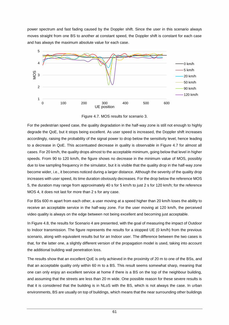
61
power spectrum and fast fading caused by the Doppler shift. Since the user in this scenario always
moves straight from one BS to another at constant speed, the Doppler shift is constant for each case
and has always the maximum absolute value for each case.
Figure 4.7. MOS results for scenario 3.
For the pedestrian speed case, the quality degradation in the half-way zone is still not enough to highly
degrade the QoE, but it stops being excellent. As user speed is increased, the Doppler shift increases
accordingly, raising the probability of the signal power to drop below the sensitivity level, hence leading
to a decrease in QoE. This accentuated decrease in quality is observable in Figure 4.7 for almost all
cases. For 20 km/h, the quality drops almost to the acceptable minimum, going below that level in higher
speeds. From 90 to 120 km/h, the figure shows no decrease in the minimum value of MOS, possibly
due to low sampling frequency in the simulator, but it is visible that the quality drop in the half-way zone
become wider, i.e., it becomes noticed during a larger distance. Although the severity of the quality drop
increases with user speed, its time duration obviously decreases. For the drop below the reference MOS
5, the duration may range from approximately 40 s for 5 km/h to just 2 s for 120 km/h; for the reference
MOS 4, it does not last for more than 2 s for any case.
For BSs 600 m apart from each other, a user moving at a speed higher than 20 km/h loses the ability to
receive an acceptable service in the half-way zone. For the user moving at 120 km/h, the perceived
video quality is always on the edge between not being excellent and becoming just acceptable.
In Figure 4.8, the results for Scenario 4 are presented, with the goal of measuring the impact of Outdoor
to Indoor transmission. The figure represents the results for a stopped UE (0 km/h) from the previous
scenario, along with equivalent results but for an Indoor user. The difference between the two cases is
that, for the latter one, a slightly different version of the propagation model is used, taking into account
the additional building wall penetration loss.
The results show that an excellent QoE is only achieved in the proximity of 20 m to one of the BSs, and
that an acceptable quality only within 60 m to a BS. This result seems somewhat sharp, meaning that
one can only enjoy an excellent service at home if there is a BS on the top of the neighbour building,
and assuming that the streets are less than 20 m wide. One possible reason for these severe results is
that it is considered that the building is in NLoS with the BS, which is not always the case. In urban
environments, BS are usually on top of buildings, which means that the near surrounding other buildings
1
2
3
4
5
0 100 200 300 400 500 600
MO
S
UE position
0 km/h
5 km/h
20 km/h
50 km/h
90 km/h
120 km/h

62
probably have LoS with the BS. Another possible reason is that the model does not take into account
the possibility of the UE being nearby a window, which means that these results would not be so harsh
for the case of a user being in a room with a window. Also, the use of the 1 800 MHz band should be
considered instead of the 2 600 MHz one for these simulations, due to the impact on path loss. Another
way to improve these results would be using a lower MCS index. Under poor channel conditions, a lower
order modulation makes the signal more resilient to errors, hence resulting in a better QoE. The cost of
this measure would be a lower throughput, meaning less TV channels available. Due to the additional
wall penetration loss, results were expected to be lower than for the outdoor case, but probably not this
lower. In conclusion, this result is not acceptable, as it suggests that eMBMS is not viable for indoors.
Figure 4.8. MOS results for scenario 4.
Making a rough estimation of how these results could be if the1 800 MHz band was used instead, based
on Figure 4.6, one can see that the 1 800 MHz band has a coverage approximately 100 m larger than
the 2 600 MHz one. If that would be the case, the coverage for an acceptable service would increase to
approximately to 120 m, which is still not good, but considerably better. If indoor coverage remains
limited to 120 m, it means that only 40% of the cell (in terms of radius, not area) is covered, which is still
far below the objective of 90%. As for the gain in coverage by considering a lower MCS index, the only
results collected that allow such analysis are the ones obtained for comparison with the measurements
described in the following section. These results are presented in Figure E.13, and represent the
variation of MOS as a user is moving away from an eNB, for each of the MCS indexes tested. This
makes the estimation even rougher, knowing that these results were obtained for a moving outdoor
user, in the 2 600 MHz band. Even so, the objective of using these results is not to know the absolute
coverage for each MCS index, but the difference between them. The figure shows that decreasing the
MCS index from 24 to 15 leads to a gain in coverage for MOS 4 of approximately 80 m. By adding 80 m
to the estimated 120 m from the change of frequency band one gets a coverage of 200 m, which
represents 60% of the cell radius, significantly better than previously, but still below the objective.
The results for Scenario 5 are presented in Figure 4.9, where the impact of the MCS index is assessed,
being motivated by the measurements presented in the next section, which were performed prior to the
development of the parametric scenarios being analysed in the current section. With the exception of
the first value presented in the figure, one can observe that the video quality decreases as the MCS
index is increased. This is due to the fact that, as the MCS index is increased, the available throughput
increases, but the transmission is less robust to errors. As the scenario is simulated with the same video
1
2
3
4
5
0 50 100 150 200 250 300 350 400 450 500 550 600
MO
S
UE position [m]
Outdoor
Indoor
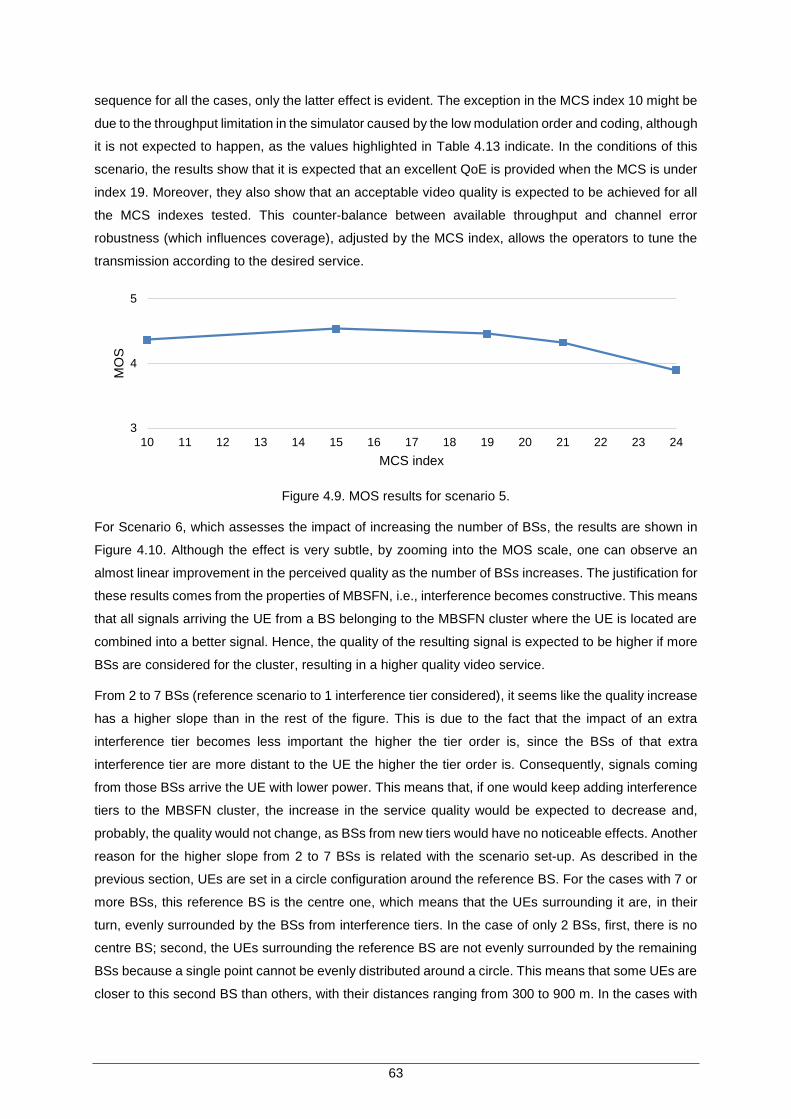
63
sequence for all the cases, only the latter effect is evident. The exception in the MCS index 10 might be
due to the throughput limitation in the simulator caused by the low modulation order and coding, although
it is not expected to happen, as the values highlighted in Table 4.13 indicate. In the conditions of this
scenario, the results show that it is expected that an excellent QoE is provided when the MCS is under
index 19. Moreover, they also show that an acceptable video quality is expected to be achieved for all
the MCS indexes tested. This counter-balance between available throughput and channel error
robustness (which influences coverage), adjusted by the MCS index, allows the operators to tune the
transmission according to the desired service.
Figure 4.9. MOS results for scenario 5.
For Scenario 6, which assesses the impact of increasing the number of BSs, the results are shown in
Figure 4.10. Although the effect is very subtle, by zooming into the MOS scale, one can observe an
almost linear improvement in the perceived quality as the number of BSs increases. The justification for
these results comes from the properties of MBSFN, i.e., interference becomes constructive. This means
that all signals arriving the UE from a BS belonging to the MBSFN cluster where the UE is located are
combined into a better signal. Hence, the quality of the resulting signal is expected to be higher if more
BSs are considered for the cluster, resulting in a higher quality video service.
From 2 to 7 BSs (reference scenario to 1 interference tier considered), it seems like the quality increase
has a higher slope than in the rest of the figure. This is due to the fact that the impact of an extra
interference tier becomes less important the higher the tier order is, since the BSs of that extra
interference tier are more distant to the UE the higher the tier order is. Consequently, signals coming
from those BSs arrive the UE with lower power. This means that, if one would keep adding interference
tiers to the MBSFN cluster, the increase in the service quality would be expected to decrease and,
probably, the quality would not change, as BSs from new tiers would have no noticeable effects. Another
reason for the higher slope from 2 to 7 BSs is related with the scenario set-up. As described in the
previous section, UEs are set in a circle configuration around the reference BS. For the cases with 7 or
more BSs, this reference BS is the centre one, which means that the UEs surrounding it are, in their
turn, evenly surrounded by the BSs from interference tiers. In the case of only 2 BSs, first, there is no
centre BS; second, the UEs surrounding the reference BS are not evenly surrounded by the remaining
BSs because a single point cannot be evenly distributed around a circle. This means that some UEs are
closer to this second BS than others, with their distances ranging from 300 to 900 m. In the cases with
3
4
5
10 11 12 13 14 15 16 17 18 19 20 21 22 23 24
MO
S
MCS index

64
7 or more BSs, the worst case UE is the one being at the same distance from two tier 1 BSs. In this
case, this UE is at 300 m from the centre BS (as they all are) and at approximately 370 m from the two
tier 1 BSs. Even if there was only 1 (not 7) extra BS, the UE-BS distance in this worst case UE would
be close to the 2 BS best case UE.
Figure 4.10. MOS results for scenario 6.
In Figure 4.11, the results for Scenario 7 are presented, showing the same curve from Scenario 6 along
with a new one obtained under similar conditions, with the only exception of MBSFN being now disabled.
The main property of these networks is the fact that interference becomes constructive, unlike other
situations, and being it disabled means that interference is destructive as usual. As a consequence,
each UE will be receiving unwanted signals from the surrounding BSs, in the same frequency in which
the UE is receiving his wanted signal, probably a delayed version of the wanted signal, since all users
in the network are using the same service. This makes it difficult for the UE to distinguish between his
signal and the interfering signals it receives and consequently reduces the service quality. As more
surrounding BSs are considered, more sources of interfering signals exist, hence poorer service quality.
As a result of this, nearly the opposite of what happened in scenario 6 is expected and verified to happen
now. As can be seen in the figure, the same higher slope from 2 to 7 BSs exists, but no zooming is
needed now for it to be noticeable. The reasons for this are the same as for scenario 6, although the
slope is much higher now than in Scenario 6, because in this scenario the quality was already acceptable
and MOS was not that far from the maximum value of 5.
Figure 4.11. MOS results for scenario 7.
In Scenario 6, for the 2 BS case, each UE was 300 m away from the closest BS. By adding the first
4,0
4,1
4,2
4,3
4,4
4,5
0 5 10 15 20 25 30 35 40
MO
S
Number of BSs
1
2
3
4
5
0 5 10 15 20 25 30 35 40
MO
S
Number of BSs
MBSFN ON
MBSFN OFF

65
interference tier, at least one of the new BSs is, at most, 370 m away from the UE. This means that the
UE is receiving new signals with power similar, but lower, to the one coming from the closest BS. This
fact, together with the fact that video quality was already good, implies that the quality raise is not much
relevant. In this scenario, receiving multiple unwanted signals with power similar to the wanted signal
creates a much higher impact because the receiver has to distinguish between the two (or more). As
the number of interference tiers is increased, the impact of each tier is lower for the same reasons
explained for Scenario 6.
The impact of increasing the number of BSs in this scenario becomes worse knowing that no frequency
re-use schemes are considered and that BSs are omnidirectional by default.
The realistic scenarios intent to exhibit the results obtained for the parametric scenarios in more realistic
scenario configurations, with BS positions based in a real life network and a higher number of users with
different channel conditions. The results for the urban and rural scenarios are presented in Figure 4.12
and Figure 4.13, respectively. The reason for dividing the results in two parts for each scenario is that 3
different cases are assessed and in two of them the variable parameter is distance, whereas in the third
it is speed. In each of the figures, each square represents the MOS of the 5 users in very similar channel
conditions over the whole simulated time. For example, the first square in the red curve of Figure 4.12.a)
represents 5 UEs forming a pentagon with the reference BS at its centre. Although they are all 50 m
away from this centre BS, they are at different distances to the surrounding BSs. Nevertheless, since
the centre BS is the closest to the UEs, it is the one that has the major impact in MOS. For the UEs
moving case, each of the 5 users moving at the same speed is at a different position, hence experiencing
different channel conditions.
a) UEs stopped. b) UEs moving.
Figure 4.12. MOS results for Realistic Urban scenario.
Regarding the urban scenario, the red line in Figure 4.12.a) shows that, for the users being closer to the
centre BS the perceive quality is slightly lower (although always staying within the perfect interval) than
for the users being in a zone in between BSs, because they are always well covered by the some of the
large number of BSs in the scenario. In fact, some of the users who are 250 m away from the centre BS
(whose MOS is represented by the last square in the red line) are less than that distance away from a
tier 1 BS. Thus, it would not be surprising if MOS would start increasing in the highest distance values
simulated. As a matter of fact, MOS would be expected to raise if larger distances were tested, since
users would be getting closer enough to tier 1 BSs. As for the blue line in the same figure, it represents
1
2
3
4
5
0 100 200 300
MO
S
UE-BS distance [m]
Indoor
Outdoor
1
2
3
4
5
0 30 60 90 120
MO
S
UE speed [km/h]
Mobility

66
users in the same configuration as before, but now indoors. In this case, the perceived quality rapidly
decreases for users who are at larger distances to the centre. This figure represents the same
assessment as made for scenario 4. In fact, despite having different network configuration in terms of
BSs positioning, Figure 4.12.a) show high resemblance with Figure 4.8. Two subtle differences can be
observed between the figures: first, in the realistic case, the acceptable quality level is achieved for a
slightly larger distance; second, in the realistic case, MOS never exactly reaches 1. The explanations
for both aspects might be the same: there are more BSs in the realistic case and the average inter-BS
distance is marginally shorter than in the parametric scenario. The minor increase in MOS in the end of
the blue line proves what was said to be expected for the outdoor case. The fact that this increase is
verified in the indoor case and not in the outdoor, knowing that UEs in both cases have the same channel
conditions, might have to do with the difference between the propagation models for indoor and outdoor.
The same analysis of coverage estimation for the indoor case that was made for Scenario 4 can, and
must, be made here. In this scenario, it would result in coverage increasing from approximately 70 m to
250 m, corresponding to approximately 91% of cell radius coverage, since the average inter-BS distance
for this scenario is approximately 550 m. With this correction, the result is already within the objective
cell coverage of 90%. The results for the moving users in this scenario are represented by a green line
in Figure 4.12.b). The fact that, even for low speeds, the MOS does not reach 5 is explained by the fact
that the 5 users in each case move along parallel trajectories 250 m apart from each other. This means
that each of these five users has different channel conditions, in some cases moving in zones away
from any BS, as can be seen in Figure 4.3. This is compensated by the fact that other UEs always move
close to one or more BSs. As a result, the perceived quality is always acceptable. This figure can be
seen as different way of representing the same type of results as the ones obtained for Scenario 3.
There, several lines represented the instantaneous video quality as a user moved. Now, each square
represents the average quality of five users during the whole run. Despite of this, the results from both
scenarios are coincident. Figure 4.7 shows drops in quality in the same position, but more severe as
higher the user speed is. This means that the average quality of the run decreases as speed increases,
which is verified in Figure 4.12.b).
As mentioned before, in rural environments coverage is the main concern, since there is not usually a
number of users large enough to overflow network capacity. Additionally, path loss is lower than in urban
environments, due to absence of tall buildings, which justifies that BSs are more separated in rural than
in urban environments, as can be seen by comparing Figure 4.3 and Figure 4.4. Consequently, larger
UE-BS distances were considered for this scenario, in comparison with the urban scenario. For this
scenario, UE-BS distances up to 2 km for the indoor case and up to 5 km for the outdoor are considered,
which, in the latter, correspond to half of the typical distance between BSs. The results for this scenario
are presented in Figure 4.13. Looking at the a) side of the figure, the most obvious result is that the
coverage for indoor UEs is immensely lower than for outdoor UEs. An acceptable service quality is
achieved for up to approximately 600 m apart from a BS, in the case of indoor users, whereas for the
outdoor ones, that the maximum distance increases to approximately 3 km. This means that the
coverage for an acceptable video quality is approximately 5 times higher outdoor than it is indoor. In this
scenario, both cases represent not acceptable results. If one considers the inter-BS distance to be

67
10 km, consequently the cell radius to be 5 km, the cell coverage for an acceptable service quality is
merely 12% and 60% for the indoor and outdoor cases, respectively. In this scenario, one cannot make
the same approximation made for the previous indoor scenarios, first, because the lowest frequency
band is already being used, and second, because there are no results collected for the influence of MCS
index in rural environments. Even so, it is expected that the decrease of the MCS index brings the cell
coverage percentages to more acceptable values.
a) UEs stopped. b) UEs moving.
Figure 4.13. MOS results for Realistic Rural scenario.
Comparing this figure with the equivalent for the urban scenario, Figure 4.12.a), the most obvious
difference in the lines representing the outdoor case is that, where in the rural scenario MOS decreases
to 1, in the urban one there is no significant drop in quality. The seemingly most evident reason for this
fact is that the distances tested are not the same in both scenarios. However, for each scenario, the
maximum distance tested is approximately half of the typical distances between BSs for that scenario,
which means that in that case, UEs are in the middle distance between BS. The explanation for this
difference can be taken from the results in Figure 4.5 and Figure 4.6. The urban scenario uses the
2600 MHz band, and BS-BS distance is, on average, approximately 500 m. From Figure 4.5, one can
see that, with such distance, MOS is still far from dropping above 5, and in this scenario only 2 BSs
were considered. The equivalent results for the 800 MHz band used in the rural scenario, represented
in Figure 4.6, show that MOS never quite reaches 5 and drops below 4 when BSs are approximately
2 km apart, whereas BSs in the rural scenario are, on average, approximately 8 km apart.
The results for the case of UEs moving are presented in Figure 4.13.b). The figure shows that MOS is
almost constant, with a very subtle decrease as the UE speed in increased, showing similarity with its
equivalent for the urban scenario presented in Figure 4.12.b). The fact that the rural line is almost
constant at a lower value than the urban one is justified with the same arguments as for the differences
for the outdoor stopped case and also based on the results from Figure 4.5 and Figure 4.6. In the urban
scenario, the moving UEs are positioned up to 500 m away from the centre BS (which means that they
may be less than that value away from some tier 1 BS), hence their perceived quality is near perfect. In
the rural scenario, these UEs are now positioned up to 2 km, which means that the quality of the video
they receive is on the edge of not being acceptable.
1
2
3
4
5
0 1 2 3 4 5
MO
S
UE-BS distance [km]
Indoor
Outdoor
1
2
3
4
5
0 30 60 90 120
MO
S
UE speed [km/h]
Mobility

68
4.3 Measurements
4.3.1 Procedure
On April 11th, 14th and 15th, 2014, an assessment of a real functioning eMBMS service was performed
at Optimus Telecomunicações (now called NOS Comunicações, [Tele14]) headquarters in Parque das
Nações, Lisbon. This assessment consisted of measuring the quality of the received signal on the UE
and correlating it with the subjective quality of the video being played, for 5 different MCS indexes.
One BS was installed on the building with a Baseband Unit (BBU) on the ground floor, connected via
optical fibre to a Radio Remote Unit (RRU) on the 1st floor, both provided by Huawei. An in-building
Distributed Antenna System (DAS) transports the signal from the RRU to the antennas located in the 1st
to 4th floors of the 10-storey building, as show in Figure 4.14. Measurements were made at 60 different
points for each MCS index, in the 2nd and above floors of the building, as shown in the figure, using an
UE, also provided by Huawei, connected to a laptop via the USB port. The low number of points is due
to time restrains since the equipment was available for just a few days. Initially, points were taken in
several sites spread over a floor, but then it was noticed that the position along the same floor did not
have significant influence on the measured values. It was also noticed that the position of the UE on the
top of the laptop keyboard strongly affected those values. After noticing there aspects, points were
taken, at each floor, only in dining rooms (inside) and stairways (outside), with the exception of the 2nd
floor, where a few points were taken at Engr. Ricardo Dinis’ desk. In all the cases, points were taken
with the UE being held on a hand, on the top of a table and on the top of the laptop keyboard. Real-time
values of the SNR, RSRP, RSRQ and Received Signal Strength Indicator (RSSI) received at the UE
were read from a data acquisition software tool installed on the laptop, where, [HoTo09]:
RSRP is the average power measured (and the average between receiver branches), for a
particular cell, of the resource elements that contain cell-specific reference signals.
RSSI is the total received wideband power on a given frequency;
RSRQ is the ratio of the RSRP and the E-UTRA Carrier RSSI, for the reference signals;
These measurements, especially RSRP, are fundamental for the UE’s cell selection and reselection
procedures and also for operators when designing cellular networks. RSRP, RSRQ and RSSI can be
related according to:
𝑅𝑆𝑅𝑄[dB] = 10 log10 (𝑁𝑅𝐵
𝑅𝑆𝑅𝑃
𝑅𝑆𝑆𝐼) (4.1)
= 10 log10(𝑁𝑅𝐵) + (𝑅𝑆𝑅𝑃[dBm] − 𝑅𝑆𝑆𝐼[dBm]) (4.2)
where:
𝑁𝑅𝐵 is the number of RBs allocated.
Unfortunately, only on the last day of measurements, the author realised that the software tool allowed
to read real-time values for received throughput, therefore results with throughput are only available for
the highest MCS index tested. Even though, it is not expected that the MCS index would have influence

69
on the throughput figures. In the reading of the throughput values, since these show fast and wide
variations, data acquisition had to be frozen so a consistent reading could be made (i.e., throughput at
a lower layer has to be higher than the throughput at a higher layer). For the remaining values this was
not necessary, since the values were usually stable enough for an accurate reading.
a) Floor plan b) Vertical cut
Figure 4.14. Approximate building plan with BSs locations and measurement positions
The UE was playing a live TV channel, from the few available, in MPEG Transport Stream (MPEG-TS)
with the video coded in H.264/AVC and the audio coded in MPEG-2. On the first day, six TV channels
were available, although only two were used – SIC Notícias (news) and Discovery Channel (science
documentary/reality shows). On the following days, only one channel was available – SIC Notícias since
the MCS index was lowered and such reduction results in lower throughput and, consequently less
supported channels.
At each point, the values mentioned above, shown on the software tool, and the floor at which they were
taken were registered and a subjective evaluation of the video quality was made, based on a 5-grade
MOS scale and according to the criteria in Table 4.12. On the first day of measurements, points were
taken for two TV channels in each site, so that the change in the content could result in different scores
for the same SNR.
Table 4.12. MOS scale and evaluation criteria.
MOS Quality Experience
5 Excellent Perfect
4 Good A few image disruptions and very occasional blocking. Not annoying
3 Fair Content is perceptible, but annoying to watch
2 Poor A few images, but content hard to understand
1 Bad No service at all

70
After 60 measurement points taken at each MCS index, the index was changed according to Table 4.13,
where the MCS indexes used in the measurements are highlighted. The MCS indexes used were:
𝐼𝑀𝐶𝑆 = 19, on the first day;
𝐼𝑀𝐶𝑆 = 10, 15 and 21, on the second day;
𝐼𝑀𝐶𝑆 = 24, on the third day.
Table 4.13. Modulation, TBS index, Throughput and number of channels.
MCS Index 𝐼𝑀𝐶𝑆
Modulation Order
𝑄𝑚
TBS Index 𝐼𝑇𝐵𝑆
Coding Rate
TBS [Bits]
Throughput [Mbps]
Available Channels
3 2 3 0.25 5736 3.44 1
4 2 4 0.30 7224 4.33 1
5 2 5 0.37 8760 5.26 1
6 2 6 0.34 10296 6.18 2
7 2 7 0.52 12216 7.33 2
8 2 8 0.59 14112 8.47 2
9 2 9 0.67 15840 9.50 3
10 4 9 0.33 15840 9.50 3
11 4 10 0.37 17569 10.54 3
12 4 11 0.43 19848 11.91 3
13 4 12 0.48 22920 13.75 4
14 4 13 0.54 25456 15.27 5
15 4 14 0.60 28336 17.00 5
16 4 15 0.64 30576 18.35 6
17 6 15 0.43 30576 18.35 6
18 6 16 0.46 32856 19.71 6
19 6 17 0.51 36696 22.02 7
20 6 18 0.55 39232 23.54 7
21 6 19 0.60 43816 26.29 8
22 6 20 0.65 46888 28.13 9
23 6 21 0.70 51024 30.61 10
24 6 22 0.75 55056 33.03 11
25 6 23 0.80 57336 34.40 11
26 6 24 0.85 61664 37.00 12
27 6 25 0.89 63776 38.27 12
28 6 26 0.93 75376 45.23 15
The first three columns in Table 4.13 are extracted from [3GPP09b]. The values in the fourth column,
the Transport Block Size (TBS), are also obtained from [3GPP09b], considering that the number of RBs
allocated is 100. The fifth column is the total throughput available for channels, being obtained from:

71
𝑅𝑏[Mbps] =𝑇𝐵𝑆[Bits]
𝜏𝑇𝑇𝐼[ms]
∙6
10∙
1
106 (4.3)
where:
the 6
10 term represents the maximum fraction of subframes out of a radio frame that are used for
eMBMS, [RoSc11].
The maximum number of channels, on the sixth column, is easily obtained dividing the total available
throughput by the maximum channel throughput and knowing that each channel has a maximum
throughput of 3 Mbps.
The interest of using lower MCS indexes is to broadcast one single channel (or very few) to a large area,
since it is expected that the same score is achievable with a lower SNR comparing to the case of higher
MCS indexes. Consequently, a larger number of users are covered. On the other hand, using higher
MCS indexes allows for a higher throughput and consequently more channels, but it is expected to
require better radio channel conditions (higher SNR), comparing to lower MCS indexes, to keep the
same score. For that reason, this case is more appealing to services in small areas, such an indoor or
home services, where a user can enjoy a large number of channels.
4.3.2 Results
The values read from the software tool and the subjective quality values were stored on a spreadsheet
and later converted into graphs, such as showed in Figure 4.15, where, for each MCS index, the SNR
and the subjective quality values of each measurement point are represented by black dots, as well as
a logistic trend line that makes an approximation of the real dependency of MOS on SNR.
By analysing the black dots only, in any of the graphs, one can observe three distinct zones: a first zone
where all the points have an MOS of 1, no matter how small SNR is, since this is the lowest score
possible; a second zone where, as expected, the MOS increases approximately linearly with SNR; and
a third zone where all the points have an MOS of 5, no matter how large SNR is, since this is the highest
score possible. The function that best approximates this behaviour is a logistic function – an S-shaped
function with an initial exponential growth that is eventually saturated by an exponential decay following
an approximately linear growth. The logistic trend lines are represented in Figure 4.15 by blue lines, with
the corresponding function and the square of the sample Pearson’s correlation coefficient, 𝑅2. As one
can observe, all but one of the trend lines have a correlation coefficient above 0.9, proving this is a good
approximation. The trend line of figure having a lower correlation coefficient may result from the large
range of SNR values that were collected with scores of 3 and 4.
More interesting than reading the 5 figures above separately, as they all look similar, is to merge them
and to analyse the differences between them, i.e., to analyse the impact of the changing of MCS index
in the MOS vs. SNR curves. Consequently, the trend lines for the five figures were merged into a new
one represented in Figure 4.16. Analysing the trend lines in the figure together, one can observe that
they all have approximately the same slope in zone two, which means that the score is affected equally
by variations (not absolute values) in SNR for all MCS indexes.

72
a) 𝐼𝑀𝐶𝑆 = 10
b) 𝐼𝑀𝐶𝑆 = 15
c) 𝐼𝑀𝐶𝑆 = 19
d) 𝐼𝑀𝐶𝑆 = 21
1
2
3
4
5
-10 0 10 20 30 40 50
MO
S
SNR [dB]
y=1+4/(exp(3.82675-0.282924*x))R²=0.910781
1
2
3
4
5
-10 0 10 20 30 40 50
MO
S
SNR [dB]
1
2
3
4
5
-10 0 10 20 30 40 50
MO
S
SNR [dB]
1
2
3
4
5
-10 0 10 20 30 40 50
MO
S
y=1+4/(exp(6.35996-0.415293*x)) R²=0.910781
y=1+4/(exp(6.43992-0.392449*x)) R²=0.935039
y=1+4/(exp(7.2333-0.370645*x)) R²=0.848511

73
e) 𝐼𝑀𝐶𝑆 = 24
Figure 4.15. MOS vs. SNR figures, with logistic trend lines, for five different MCS indexes.
On average, an increase of approximately 3 dB in SNR results in the score increasing by 1. More
interesting than that, one can also observe that the lower the MCS index is, the closer the correspondent
curve is to the vertical axis, and vice-versa. This demonstrates that, as expected, in order to keep a
constant score, as the MCS index is increased, the radio channel conditions (i.e., SNR) have to increase
as well. Analysing this from another angle, for a constant SNR, an increase in the MCS index results in
a degradation of the video quality and therefore in a lower score.
Figure 4.16. Logistic trend lines for the measurements results.
An important aspect that one should be able to take from this figure is the minimum SNR required to
achieve a given MOS. Taking such information from this figure may be inaccurate for three reasons:
first, the low number of measurement points might not allow the lines to be representative of the real
scenario; second, the trend lines are approximations to the measurement points and, as can be
observed in Figure 4.15, they are not always good approximations in the transitions between the
mentioned zones; third, as can also be observed in Figure 4.15, it might occur that, for the a constant
MOS, some points are enough apart from the average SNR that they are probably causing the trend
line to deviate from the zone with higher concentration of points where it was supposed to cross. These
points may have been cause by measurement or equipment errors, or even by rare reception conditions,
and their influence on the results should be minimised. The only solution to the first issue would be to
take more points, but unfortunately that was not possible. In order to overcome the other issues, the
bars in Figure F.1 represent the interval between the 5th and 95th percentiles of the SNR values for each
1
2
3
4
5
-10 0 10 20 30 40 50
MO
S
SNR [dB]
1
2
3
4
5
-10 0 10 20 30 40 50
MO
S
SNR [dB]
MCS=10
MCS=15
MCS=19
MCS=21
MCS=24
y=1+4/(exp(8.14931-0.363063*x)) R²=0.918355

74
score and each MCS index and the error lines represent the whole interval of values. In this
representation, the influence in the results of a point that is apart from the majority is reduced. Since
operators usually aim to provide the user a service with a quality corresponding to a score of 5, the most
important measure to take from the figure is the minimum SNR required to achieve an MOS of 5.
Therefore, looking at the lower bounds of the bars in Figure F.2.e), one can observe that the required
SNR is higher as higher the MCS index is (although not always clear in the results mainly due to the low
number of points), and that it ranges between approximately 20 dB and 28 dB for the tested MCS
indexes. If such analysis was based on the trend lines in Figure 4.16 the interval would be between
approximately 24 dB and 31 dB, which is not accurate as one can see from the points in Figure 4.15.
Another aspect that is interesting to analyse is how the quality of the video experienced by the user,
reflected in the MOS, changes over the building floors. The averages of the scores (MOS) of all the
measurement points in each floor and for each MCS index are represented in Table 4.14, where the
highest scores are highlighted in darker blue and the lowest scores in lighter blue or not highlighted at
all. For the MCS index of 10, points were not taken in the first three floors due to lack of relevance, i.e.,
for a low MCS index, it is worthless to take many points close to a BS, as they will all have a score of 5.
Table 4.14. MOS for each MCS index and at each building floor.
Floor 𝐼𝑀𝐶𝑆=10 𝐼𝑀𝐶𝑆=15 𝐼𝑀𝐶𝑆=19 𝐼𝑀𝐶𝑆=21 𝐼𝑀𝐶𝑆=24
9 2,00 1,25 1,55 1,17 1,00
8 2,09 2,29 1,67 1,67 1,00
7 2,83 2,73 2,50 2,21 1,33
6 3,50 3,50 3,00 2,43 1,80
5 4,07 3,45 3,80 3,20 2,67
4 - 5,00 5,00 4,50 3,70
3 - 4,67 4,27 3,75 3,72
2 - 5,00 5,00 4,80 3,80
As expected, the 2nd and 4th floors are the ones with the highest MOSs for all the MCS indexes, as those
are the floors where the two BSs are located. It is also expected and verified that the 3rd floor is the floor
without BS with the highest MOS, since it is between two floors with BSs. Also, as obvious, as the user
ascends the building from the 4th floor upwards, the quality of the video decreases, since the UE is
moving away from the closest BS. Finally, as one looks at the table from another angle, it is possible to
see that, in every floor, the increase in the MCS index decreases the video quality and so the MOS.
As for the throughput, values are available for the MCS index of 24 only, for the reasons mentioned
above. As also mentioned before, each channel has a throughput of 3 Mbps, and that is verified through
Figure 4.17. The blue line in the figure is a logistic trend line, which again has proved to be the best
approximation to the points represented as black dots, corresponding to the throughput at the Packet
Data Convergence Protocol (PDCP) layer. As shown in the figure, when in good reception conditions,
i.e., for an SNR higher than approximately 22 dB, the total channel throughput is received by the UE.
On the other hand, when the SNR is lower than approximately 16 dB, nothing is received on the UE.

75
Figure 4.17. Influence of the SNR in the received throughput.
Another interesting aspect to analyse concerning the received throughput is related with the MOS. Such
relation is represented in Figure 4.18. Again, a logistic trend line is represented by a black line, as an
approximation to the points representing the PDCP throughput.
Figure 4.18. Relation between the received throughput and the MOS.
An observation to the figure is that, for an MOS of 5 the UE must receive the total channel throughput.
This was expected since, from the definition of the maximum score, the video must be perfect, without
any image disruptions or blocking, and that is only achievable if the UE is able to receive the whole data.
With the exception of a few points, even for an MOS of 4 the UE requires almost the total throughput.
Those exception points may have occurred during a period when the video content had low motion.
Another comment is that approximately 90% of the channel total throughput must be received at the UE
in order to achieve a Fair (MOS of 3) video quality. If anything (or almost) is received at the UE, no
service is provided and therefore the score should not be higher than 1.
4.4 Comparison of Simulation and Measurement results
In this section, the results obtained from simulations are compared with the results obtained from
measurements described in Section 4.3. The purpose of this comparison is to establish a link between
simulations and real world, and to examine where the two differ. Seeing that the main analysis made for
the measurements results focuses on the impact of the variation of the MCS index in the perceived
0
1
2
3
4
-10 0 10 20 30 40 50
Thro
ughput
[Mbit/s
]
SNR [dB]
0
1
2
3
4
1 2 3 4 5
Thro
ughput
[Mbit/s
]
MOS
y=3/(exp(15.8166-0,806195*x)) R²=0.890829
y=3/(exp(7.0944-3.147595*x)) R²=0.943484

76
quality, by means of analysing the required SNR for each quality score to be achieved, comparison with
the simulations is only possible having equivalent results obtained from simulations. Among the
scenarios described in Section 4.1 there is in fact one scenario where the impact of the variation of the
MCS index is assessed, but no SNR statistics were collected from the simulation of that scenario.
Therefore, one cannot use any of the simulation results to make the comparison with the measurements,
thus new simulations are performed for this purpose.
As the objective of each simulation is simply to measure the impact of the SNR in the perceived quality,
for a given MCS index, a very simple scenario is configured, with only 1 eNB and 1 UE, being this UE
moving away from the eNB at the pedestrian speed of 1.5 m/s. The simulation duration was chosen as
600 s, so that the UE covers 900 m, in order to gather SNR values for all the quality scores. This scenario
is adapted from the reference scenario for the parametric simulations, hence all the parameters apart
from those that were just explained maintain their values. As seen before, more BSs improve the
perceived quality, but that happens as a direct consequence of a better channel quality, i.e., higher DL
SNR. For these new simulations, the same packet statistics are collected to be used as input for the
quality estimation model, but in addition to that, average DL SNR statistics in a 1 second window (since
this metric is fast varying) are extracted from the simulator.
The results obtained from the new simulations just described are presented in Figure E.12 in Annex E.
Each figure represents a MOS vs. SNR point per second of simulation, for a given MCS index. The five
figures presented represent the 5 five MCS indexes assessed in the measurements. In each figure is
also represented a logistic trend line that approximates the overall behaviour of the points with a logistic
equation. The equation that better fits each figure is also indicated in the respective figure, as well as
the square of the sample Pearson’s correlation between the points and the trend line approximating
them. In order for the difference between the trend lines to be noticeable, they are grouped together in
Figure 4.19. This figure is now comparable with its equivalent from the measurements, Figure 4.16.
Figure 4.19. Logistic trend lines for the simulations results.
Looking at both figures, the first reaction would be to say that they look very similar. The lines
represented do have the same shape in both figures, but that is no surprise, since they all are logistic
functions approximating the variation of MOS with SNR. In fact, if one pays attention to details, the
results presented in these figures have several differences. The major difference between the results
lies in their nature, i.e., the measurements results are based on a statistical mensuration whereas the
1
2
3
4
5
15 20 25 30 35 40 45
MO
S
SNR [dB]
MCS=10
MCS=15
MCS=19
MCS=21
MCS=24
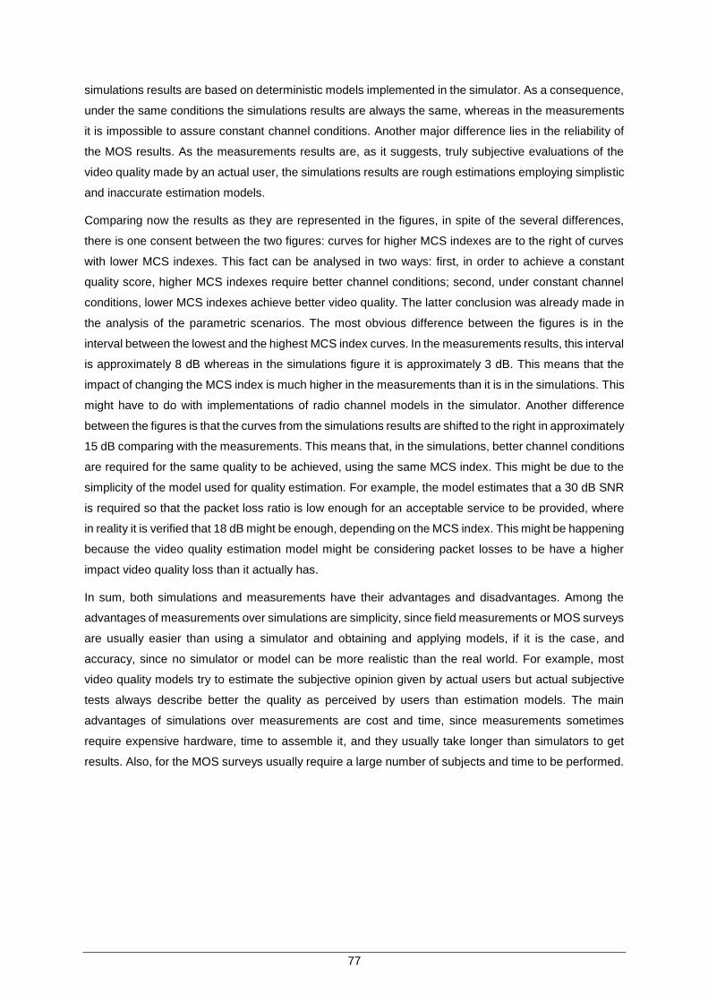
77
simulations results are based on deterministic models implemented in the simulator. As a consequence,
under the same conditions the simulations results are always the same, whereas in the measurements
it is impossible to assure constant channel conditions. Another major difference lies in the reliability of
the MOS results. As the measurements results are, as it suggests, truly subjective evaluations of the
video quality made by an actual user, the simulations results are rough estimations employing simplistic
and inaccurate estimation models.
Comparing now the results as they are represented in the figures, in spite of the several differences,
there is one consent between the two figures: curves for higher MCS indexes are to the right of curves
with lower MCS indexes. This fact can be analysed in two ways: first, in order to achieve a constant
quality score, higher MCS indexes require better channel conditions; second, under constant channel
conditions, lower MCS indexes achieve better video quality. The latter conclusion was already made in
the analysis of the parametric scenarios. The most obvious difference between the figures is in the
interval between the lowest and the highest MCS index curves. In the measurements results, this interval
is approximately 8 dB whereas in the simulations figure it is approximately 3 dB. This means that the
impact of changing the MCS index is much higher in the measurements than it is in the simulations. This
might have to do with implementations of radio channel models in the simulator. Another difference
between the figures is that the curves from the simulations results are shifted to the right in approximately
15 dB comparing with the measurements. This means that, in the simulations, better channel conditions
are required for the same quality to be achieved, using the same MCS index. This might be due to the
simplicity of the model used for quality estimation. For example, the model estimates that a 30 dB SNR
is required so that the packet loss ratio is low enough for an acceptable service to be provided, where
in reality it is verified that 18 dB might be enough, depending on the MCS index. This might be happening
because the video quality estimation model might be considering packet losses to be have a higher
impact video quality loss than it actually has.
In sum, both simulations and measurements have their advantages and disadvantages. Among the
advantages of measurements over simulations are simplicity, since field measurements or MOS surveys
are usually easier than using a simulator and obtaining and applying models, if it is the case, and
accuracy, since no simulator or model can be more realistic than the real world. For example, most
video quality models try to estimate the subjective opinion given by actual users but actual subjective
tests always describe better the quality as perceived by users than estimation models. The main
advantages of simulations over measurements are cost and time, since measurements sometimes
require expensive hardware, time to assemble it, and they usually take longer than simulators to get
results. Also, for the MOS surveys usually require a large number of subjects and time to be performed.

78

79
Chapter 5
Conclusions
5 Conclusions
This chapter finalises this work, summarising conclusions and suggesting aspects to be developed in
future work.

80
The main objective of this thesis was to analyse various parameters that influence the QoS of eMBMS
as perceived by end users in both urban and rural scenarios. Most of the scenarios analysed were
simplistic scenarios defined by the author with the objective of assessing the impact of specific
parameters. Two realistic scenarios based on a real network, provided by a Portuguese telecom
operator, were also analysed focusing on three different cases each. The percentage of the cell radius
in which an acceptable service can be provided and the influence of parameters such as MCS index
and user mobility was assessed.
The fundamental aspects of the technologies studied in this thesis are presented in Chapter 2. The basic
aspects of the two subjects on which this thesis lays, LTE and video streaming, are discussed,
concluding with the state of the art of video transmission over LTE networks. The first section describes
the fundamental aspects of LTE, focusing on its network architecture, where the basic structure and
functions of its main nodes are explained; the LTE radio interface, where details regarding frequency
bands, bandwidths, frame structure and resource allocation are provided; a capacity study, based on
the theoretical peak data rates. The next section briefly presents the main services and applications
supported by LTE and their classifications, with concepts of QoS being addressed. The following section
presents the basics of video coding and transmission, specifically on the H.264/AVC standard. The
fourth section present the subject that serves as the main motivation for this thesis, eMBMS. Its
properties and basic concepts are presented and its main advantages against common unicast video
streaming services are discussed. The following section presents the main parameters that affect the
performance of video transmission over LTE networks, i.e., the types of metrics used to assess video
quality and which parameters have influence them. The sixth and final section of this chapter presents
the state of the art on this subject, where studies by other authors on video transmission over LTE and
commercial deployment of eMBMS are presented.
The simulator and models used in this thesis are explained in Chapter 3. The simulator is presented and
all aspects regarding the models are described. Then, the configuration of the simulator and the
implementation and use of the models are described. The chapter is concluded with an assessment of
the models and simulator. The first section describes the simulator used in this thesis. This simulator
was neither developed nor edited by the author of this thesis, being the work regarding the simulator
narrowed to understanding and configuring it properly. Hence, this section provides a brief description
of the simulator’s structure, node attributes and results statistics that it collects. The second section
describes the radio link model implemented in the simulator. The information on this section was based
on the simulator’s documentation and it focuses mainly on the propagation models implemented and
physical layer measurements supported. The third section describes the video quality assessment
models used in this thesis, and the equations that define them are presented. One of the two models
presented is an improvement of the other, hence only the first is used for results analysis. Both these
models use the output of the simulator as input and return a rough estimation of the quality of video as
it would be perceived by a user watching it. The following section described the leaky bucket model,
used to determine the buffer size for a reference H.264/AVC decoder. This outcome of this model is
used by the rebuffering delay models – two simple models developed by the author of this work to
determine the probability of a video playback to stop due to missing data. The next section presents the

81
global model simulator and it is composed of three sub-sections. The first of these sub-sections
describes the configuration of the simulator, presenting the main nodes of a reference scenario and their
major attributes. This sub-section also describes how video information is inputted in the simulator for
transmission. The simulator uses as input a file containing information of video frames for a certain video
sequence and generates traffic according to it. The remaining two sub-sections describe the
implementation of the video quality estimation models and the rebuffering delay models. They are both
implemented in the same program written in C, since they both use the same results exported from the
simulator. The output is a file containing the results to be analysed further. This chapter is concluded
with a sixth section where the described models are assessed. A simple scenario is tested in order to
verify is the results are consistent with what is expected. Also, an assessment of the pre-configured
eMBMS service in the simulator is made, in order to assure that it works properly.
In Chapter 4, the results from both simulations and measurements are assessed. This chapter contains
four sections, the first being a description of the scenarios simulated, the second containing the analysis
of the results obtained from those simulations, the third describing the measurements performed and
analysing their results, and the fourth establishing a connection between simulations and measurements
results. The first section is an overall description of the scenarios simulated, starting by an extensive
description of all the parameters defining a reference scenario. Then, several parametric scenarios are
described by comparison with the reference. Finally, two realistic scenarios are described, one urban
and the other rural, both based on real LTE networks. The second section provides some of the results
obtained for each scenario, along with an analysis for each scenario. This analysis if based on an
influence of each parameter in the quality of service, with a comparison of the obtained results with what
is expected or ideal. The third section concerns the measurements performed by the author of this thesis
with an experimental set up of eMBMS, and is divided in two sub-sections. The first sub-section
describes the full measurement procedure and the conditions in which the results were obtained. The
second sub-section presents these results and analyses them, focusing on the channel condition
needed for an acceptable QoE to be provided. The fourth and last section of this chapter makes a
comparison between the simulations and measurements. In order to proper compare the results
obtained from measurements, new simulations were made for a simple scenario, where the variation of
video quality with SNR is displayed.
In this thesis, the analysis is done by simulating several scenarios and determining the conditions
necessary for an acceptable QoE to be provided or by determining the probability of such service to be
provided to a user in a specific scenario. First, 7 parametric scenarios were analysed, each one
assessing the impact in video quality of specific parameter, the 7 parameters being: inter-BS distance,
frequency band used, UE-BS distance and user mobility, outdoor-to-indoor propagation, MCS index,
number of eNBs and MBSFN usage. For each scenario, several simulations were made, for different
parameter values. The two realistic scenarios are similar in configuration, differing in the positioning of
the eNBs, frequency band and propagation model. In these simulations 3 simultaneous cases are
considered: users indoor, users stopped outdoors and users moving outdoors. For each case, 5 different
situations were tested, i.e., 5 different distances to a specific eNB, for the stopped user and 5 different
velocities for the moving users, resulting in users in 15 different situations. For each of these 15

82
situations, 5 users were considered in different positions, resulting as described before in 75 users under
different conditions.
Most of the results obtained in the parametric simulations are satisfactory. The results from the realistic
scenarios are not so acceptable, since they were obtained under adverse conditions. One should not
forget that the simulations were not performed with actual video being transmitted. The simulator simply
generates random traffic with bit rate defined by the information regarding frames sizes inputted from
the video trace file. This creates another limitation: since it is not real video that is being transmitted, it
is not real video that is being received at the UEs, hence no full-reference estimation models can be
applied. Remember that these models make a comparison between the original video sequence before
being transmitted and the damaged sequence after being received on the other end. Therefore, only
no-reference models could be used, which are sometimes less accurate. To make it even worse, most
no-reference models require the received video sequence, which was not available. That could have
been done if the original sequence had been coded by the author of this thesis and if the UE module in
the simulator could at least export a trace file of the received data. Merging this trace file with the coded
sequence would allow for a damaged sequence to be decoded, and no-reference models to be applied.
However, this feature of exporting trace files was not implemented in the UE module, and implementing
it would fall far out of the scope of this thesis. Remember that the choice of this simulator was based on
the fact that it already included simple pre-configured scenarios for eMBMS, with MBSFN already
properly implemented. This allowed the author to save plenty of work, having only to comprehend and
modify the pre-configured scenarios. With the presented limitations, extremely rough no-reference
models that rely only on packet loss ratio are the only solution.
Although the results from the measurements show a clear relationship between channel conditions,
video quality and the influence of the MCS index, these measurements were performed in an indoor
hotspot environment inside an office building, not being representative of the more common scenarios
where BSs being outside and users both indoors and outdoors.
The major outline conclusion drawn by the results is that eMBMS improves the quality of a video
streaming. The improvement in the perceived quality is clearly visible in the parametric scenario that
addresses it. One of the objectives of this thesis from the point of view of NOS was to assess whether
this service is viable and if it is worth the necessary investment. This is done by assessing whether it is
possible to provide a good QoE to all customers in different conditions and which are the necessary
conditions for that. Focusing primarily on the results from the realistic scenarios, one would be tempted
to conclude that this service is not of interest for the Portuguese operator since most indoor clients would
not be satisfied, with only 25% and 12% of the cell radius being covered with an acceptable service for
the urban and rural scenarios, respectively, under the simulated conditions. However, as already
explained, these results were obtained in very unfavourable conditions, i.e., using high modulation and
coding for both scenarios and using the frequency band with the highest path loss for the urban scenario.
As also explained, the results obtained from the parametric scenarios allow for a rough estimation of
what these percentages of coverage could be under more favourable conditions. The percentages of
satisfied users were then estimated to increase to 91% for the urban if more favourable conditions had

83
been used. No similar estimation is made for the rural scenario, since the parametric scenarios do not
provide the necessary results in this case. For the outdoor case, the results for the urban scenario show
that all users can be provided an excellent service, whereas in the rural scenario an acceptable service
can only be provided in approximately 60% of the cell radius. Again, this result is unacceptable for the
operator, but using a smaller modulation order could improve the service coverage and consequently
the percentage of satisfied clients. The impact of mobility provokes the perceived quality to slightly
decrease from near-perfect to just acceptable in urban environments, which is guaranteed to users
moving at velocities below 120 km/h. In rural environments, almost no impact is noticed, with the quality
always being just above acceptable. Again, this could be improved by choosing a lower MCS index.
Summarising these results, in the urban environment only indoor costumers can have complaints, even
in the most favourable conditions. A possible solution could be the use of indoor hotspots. In the rural
environment, all 3 cases tested have low coverage under the simulated conditions. As already
mentioned, the necessary solution is to use lower order modulation by setting a lower MCS index.
Another important conclusion is that the use of the eMBMS service in the 2600 MHz band is not advised.
Regarding future work, some notes were already made regarding limitations to simulations and
measurements. In the simulations, it would be ideal to simulate the transmission of real video sequences
so that more accurate quality estimation models could be used. Moreover, future work could assess the
advantage of eMBMS for a BS cluster with a large number of users, i.e. by assessing the impact of
increasing the number of multicast users for eMBMS both enabled and disabled. Also, the
measurements were made only on an indoor hotspot scenario. Measurements for outdoor, outdoor-to-
indoor and outdoor with mobility and in rural environments could improve this work and validate the
simulations. Also, it would be interesting to consider additional users in the network using other LTE
services. The assessment of the influence of this additional users in the QoS perceived by the eMBMS
users would be an interesting aspect to be assessed in the future.

84

85
Annex A
Link Budget
Annex A. Link Budget
In this annex, the equations that define Link budget for coverage estimation and SNR are presented.

86
Coverage is an important parameter when assessing the performance of a radio cell and Link budget is
an essential tool to estimate it. Because the basic LTE resource is the sub-carrier, coverage estimation
can done either independently for each sub-carrier or for the set of RBs allocated. A cell can be seen
as a disk, with the BS at its centre, whose radius is the maximum distance between BS and MT in which
is possible to establish communication meeting MT’s SINR requirements. Coverage is usually defined
as the maximum radius a cell can have, and it depends on the location of the cell, hence the most
suitable propagation model should be assessed. The radius of a cell can be determined using the
logarithmic form of Friis transmission equation:
𝐿𝑝[dB]= 𝑃𝑡 [dBm] + 𝐺𝑡[dBi]
− 𝑃𝑟[dBm] + 𝐺𝑟[dBi] (A.1)
where:
𝐿𝑝 is the path loss;
𝑀𝑝 is the power margin, which is the sum of margins for fast and slow fading and indoor
penetration;
𝑃𝑡 is the power fed to the transmitting antenna;
𝑃𝑟 is the power available at the receiving antenna;
𝐺𝑡 and 𝐺𝑟 are the transmitter and receiver gains, respectively.
The power fed to the BS antenna in DL is given by:
𝑃𝑡 [dBm]𝐷𝐿 = 𝑃𝑇𝑥[dBm] − 𝐿𝐶 [dB] (A.2)
where:
𝑃𝑇𝑥 is the transmitter output power;
𝐿𝐶 is the loss in the cable connecting the BS transmitter to the antenna.
The power fed to the MT antenna in UL is given by:
𝑃𝑡 [dBm]𝑈𝐿 = 𝑃𝑇𝑥[dBm] − 𝐿𝑈[dB] (A.3)
where:
𝐿𝑈 is the loss due to user’s head and hands.
The power received by the MT receiver in DL is given by:
𝑃𝑅𝑥 [dBm]𝐷𝐿 = 𝑃𝑟 [dBm] − 𝐿𝑈[dB] (A.4)
The power received by the BS receiver in UL is given by:
𝑃𝑅𝑥 [dBm]𝑈𝐿 = 𝑃𝑟[dBm] − 𝐿𝐶 [dB] (A.5)
The expression for the path loss in (A.1) can also be written as:
𝐿𝑝[dB]= 𝐿𝑝[dB]
𝑃𝑟𝑀 + 𝑀𝑝[dB] (A.6)
where:
𝐿𝑝𝑃𝑟𝑀 is the path loss obtained from the propagation model;

87
𝑀𝑝 is a sum of margins, whose expression is:
𝑀𝑝[dB]= 𝑀𝑆𝐹[dB] + 𝑀𝐹𝐹 [dB] + 𝐿𝑝𝑖𝑛𝑑[dB]
(A.7)
where:
𝑀𝑆𝐹 is the slow fading margin;
𝑀𝐹𝐹 is the fast fading margin;
𝐿𝑝𝑖𝑛𝑑 is the indoor penetration loss.
Putting together (A.1), (A.2), (A.4) and (A.6), one gets:
𝑃𝑅𝑥[dBm] = 𝑃𝑇𝑥[dBm] − 𝐿𝐶 [dB] + 𝐺𝑡[dBi] − 𝐿𝑝[dB]
𝑃𝑟𝑀 − 𝑀𝑝[dB]− 𝐿𝑈[dB] + 𝐺𝑟[dBi]
(A.8)
The SNR of the received signal can be calculated as:
𝜌𝑁[dB] = 𝑃𝑅𝑥[dBm] − 𝑁[dBm] (A.9)
SINR is given by:
𝜌𝐼𝑁[dB] = 10 log (𝑃𝑅𝑥[mW]
𝑁[mW] + 𝐼[mW]) (A.10)
where:
𝐼 is the interference power at the receiver, given by:
𝐼[mW] = ∑ 𝐼𝑖 [mW]
𝑁𝐼
𝑖=1
(A.11)
where:
𝐼𝑖 is the power from interfering signal 𝑖;
𝑁𝐼 is the number of interfering signals reaching the receiver.

88

89
Annex B
COST 231Walfisch-Ikegami
Model
Annex B. COST 231Walfisch-Ikegami Model
This annex presents the propagation model used to calculate the path loss in urban environment for
frequency bands under 2000 MHz.

90
3GPP TR 25.996 [3GPP11b] defines a spatial channel model, where the median value for the path loss
in an urban microcell scenario is based on the COST 231 Walfisch-Ikegami model, which defines
expressions for both LoS and NLoS cases. The COST 231 Walfisch-Ikegami propagation model
parameters are represented in Figure B.1:
Figure B.1. Definition of parameters for use in COST 231 Walfisch-Ikegami propagation model
(adapted from [Corr12]).
The expression in the case of LoS is:
𝐿𝐿𝑜𝑆[dB] = 42.6 + 26 log (𝑑[km]
1 km) + 20 log (
𝑓[MHz]
1 MHz) , for 𝑑 ≥ 20 m (B.1)
where:
𝑑 is the horizontal distance between the BS and the MT;
𝑓 is the frequency of the signal carrier.
The expression in the case of NLoS is:
𝐿𝑁𝐿𝑜𝑆[dB]= 𝐿0[dB]
+ 𝑚𝑎𝑥 {0, 𝐿𝑟𝑡𝑠𝑊𝐼
[dB]+ 𝐿𝑚𝑠𝑑
𝑊𝐼[dB]
} (B.2)
where:
𝐿0 is the free space path loss;
𝐿𝑟𝑡𝑠𝑊𝐼 is the loss due to diffraction and scatter from closest rooftop to MT;
𝐿𝑚𝑠𝑑𝑊𝐼 is the loss due to multiscreen diffraction from urban rows of buildings.
The expression for the free space propagation path loss is:
𝐿0[dB]= 32.44 + 20 log (
𝑑[km]
1 km) + 20 log (
𝑓[MHz]
1 MHz) (B.3)
The expression for the loss due to diffraction and scatter from closest rooftop to MT is:
𝐿𝑟𝑡𝑠𝑊𝐼
[𝑑𝐵]= −16.9 − 10 log (
𝑤𝑠[m]
1 m) + 10 log (
𝑓[MHz]
1 MHz) + 20 log (
∆ℎ𝑀𝑊𝐼
[m]
1 m) + 𝐿𝑜𝑟𝑖
𝑊𝐼 (B.4)
where:
𝑤𝑠 is the average street width;
∆ℎ𝑀𝑊𝐼
is the vertical distance from the MT to the top of the buildings;
𝐿𝑜𝑟𝑖𝑊𝐼 is the loss due to street orientation.
The vertical distance from the MT to the top of the buildings is given by:
∆ℎ𝑀𝑊𝐼
[m] = 𝐻𝐵𝑊𝐼
[m] − ℎ𝑚[m] (B.5)

91
where:
𝐻𝐵𝑊𝐼 is the average buildings height;
ℎ𝑚 is the height of the MT.
The loss due to street orientation is given by:
Lori𝑊𝐼
[dB]= {
−10 + 0.354𝜙[°], if 0° ≤ 𝜙 ≤ 35°
2.5 + 0.075(𝜙[°] − 35°), if 35° ≤ 𝜙 ≤ 55°
4.0 − 0.114(𝜙[°] − 55°), if 55° ≤ 𝜙 ≤ 90°
(B.6)
where:
𝜙 is the angle between the incident wave and the edge of the street where the MT is in.
The expression for the loss due to multiscreen diffraction from urban rows of buildings is:
𝐿𝑚𝑠𝑑𝑊𝐼
[𝑑𝐵]= 𝐿𝑏𝑠ℎ
𝑊𝐼 + 𝑘𝑎𝑊𝐼 + 𝑘𝑑
𝑊𝐼 log (𝑑[km]
1 km) + 𝑘𝑓
𝑊𝐼 log (𝑓[MHz]
1 MHz) − 9 log (
𝑤𝐵 [m]
1 m) (B.7)
where:
𝐿𝑏𝑠ℎ𝑊𝐼 is the loss due to the difference in heights between the buildings and the BS;
𝑘𝑎𝑊𝐼
is the increase of the path loss for BS antennas below the rooftops of the adjacent
buildings;
𝑘𝑑𝑊𝐼
is the dependence of the multiscreen diffraction loss versus distance;
𝑘𝑓𝑊𝐼
is the dependence of the multiscreen diffraction loss versus frequency;
𝑤𝐵 is the average building separation.
The loss due to the difference in heights between the buildings and the BS is given by:
𝐿𝑏𝑠ℎ𝑊𝐼
[𝑑𝐵]= {
−18 log (1 +∆ℎ𝐵
𝑊𝐼[m]
1 m) , for ∆ℎ𝐵
𝑊𝐼 > 0
0, for ∆ℎ𝐵𝑊𝐼 ≤ 0
(B.8)
where:
∆ℎ𝐵𝑊𝐼
is the vertical distance between the heights of the BS and the buildings, and is given by:
∆ℎ𝐵𝑊𝐼
[𝑚]= ℎ𝑏[m] − 𝐻𝐵
𝑊𝐼[m] (B.9)
where:
ℎ𝑏 is the height of the BS;
𝐻𝐵𝑊𝐼 is the buildings average height.
The expression for the increase of the path loss for BS antennas below the rooftops of the adjacent
buildings is:
ka𝑊𝐼
[dB]= {
54, for ∆ℎ𝐵𝑊𝐼 > 0
54 − 0.8∆ℎ𝐵𝑊𝐼
[m], for ∆ℎ𝐵𝑊𝐼 ≤ 0 and 𝑑 ≥ 0.5 km
54 − 1.6∆ℎ𝐵𝑊𝐼
[m]𝑑[km], for ∆ℎ𝐵𝑊𝐼 ≤ 0 and 𝑑 < 0.5 km
(B.10)
The expression for the dependence of the multiscreen diffraction loss versus distance is:

92
𝑘𝑑𝑊𝐼
[𝑑𝐵]= {
18, for ∆ℎ𝐵𝑊𝐼 > 0
18 − 15∆ℎ𝐵
𝑊𝐼[m]
𝐻𝐵𝑊𝐼
[m], for ∆ℎ𝐵
𝑊𝐼 ≤ 0 (B.11)
The expression for the dependence of the multiscreen diffraction loss versus frequency is:
𝑘𝑓𝑊𝐼
[𝑑𝐵]= {
−4 + 0.7 (𝑓[MHz]
925 MHz− 1) , medium cities, suburbs
−4 + 1.5 (𝑓[MHz]
925 MHz− 1) , metropolitan centres
(B.12)
This propagation model is valid under the following conditions:
𝑓 ∈ [800, 2000] MHz
𝑑 ∈ [0.02, 5] km
ℎ𝑏 ∈ [4, 50] m
ℎ𝑚 ∈ [1, 3] m
The shadow fading standard deviation takes values in 𝜎 ∈ [4, 7] dB.
For the 3GPP TS 25.966 urban microcell scenario, the following parameters are assumed:
ℎ𝑏 = 12.5 m;
𝐻𝐵𝑊𝐼 = 12 m;
𝑤𝐵 = 50 m;
𝑤𝑠 = 25 m;
ℎ𝑚 = 1.5 m;
𝜙 = 30°;
𝜎𝐿𝑜𝑆 = 4 dB;
𝜎𝑁𝐿𝑜𝑆 = 10 dB.

93
Annex C
M.2135 Propagation Models
Annex C. M.2135 Propagation Models
This annex presents the propagation models used to calculate the path loss in urban and rural
environments for frequency bands over 2000 MHz.

94
Report ITU-R M.2135-1 [ITUR09] defines expressions for calculating the median value for the path loss
for an Urban Microcell (UMi) scenario and for a Rural Microcell (RMa), among others. Both models are
specified in the frequency range from 2 GHz to 6 GHz.
C.1 Urban Microcell (UMi)
In the UMi scenario the height of both BS and MT antennas are assumed to be below the tops of
surrounding buildings and to be outdoors in an area where streets are laid out in a Manhattan-like grid.
This model is defined for both LoS and NLoS cases. The model also defines a case where users are
located indoor and BSs are outdoor.
Path loss in the case of LoS has two expressions, depending on the distance between MT and BS. The
first one is:
𝐿𝐿𝑜𝑆[dB] = 28.0 + 22 log10 (𝑑[m]
1 m) + 20 log10 (
𝑓[GHz]
1 GHz) , for 10 m < 𝑑 < 𝑑′𝐵𝑃 (C.1)
where:
𝑑 is the horizontal distance between the BS and the MT;
𝑓 is the frequency of the signal carrier;
𝑑′𝐵𝑃 is the breakpoint distance, given by:
𝑑′𝐵𝑃 [m] = 4ℎ′𝑏[m]ℎ
′𝑚[m]
𝑓[Hz]
𝑐[m/s] (C.2)
where:
𝑐 = 3.0 × 10⁸ m/s is the propagation velocity in free space;
ℎ′𝑏 and ℎ′
𝑚 are the effective antenna heights at the BS and the MT, given by:
ℎ′𝑏[m] = ℎ𝑏[m] − 1.0 (C.3)
ℎ′𝑚[m] = ℎ𝑚[m] − 1.0 (C.4)
where ℎ𝑏 and ℎ𝑚 are the actual antenna heights.
The second expression for the path loss in the case of LoS is:
𝐿𝐿𝑜𝑆[dB] = 7.8 + 40 log10 (𝑑[m]
1 m) + 2 log10 (
𝑓[GHz]
1 GHz)
−18 log10 (ℎ′
𝑏[m]
1 m) − 18 log10 (
ℎ′𝑏[m]
1 m)
, for 𝑑′𝐵𝑃 < 𝑑 < 5000 m (C.5)
For both LoS expressions, the shadow fading standard deviation is 𝜎 = 3 dB.
The expression in the case of NLoS is:
𝐿𝑁𝐿𝑂𝑆[dB]= 𝑚𝑖𝑛{𝐿[dB](𝑑1, 𝑑2), 𝐿[dB](𝑑2, 𝑑1)} (C.6)
where:

95
𝐿[dB](𝑑𝑘, 𝑑𝑙) = 𝐿𝐿𝑜𝑆[dB](𝑑𝑘) + 17.9 + 12.5𝑛𝑗 + 10𝑛𝑗 log10 (
𝑑𝑙[m]
1 m)
+ 2 log10 (𝑓[GHz]
1 GHz)
(C.7)
𝑛𝑗 = 𝑚𝑎𝑥 {2.8 − 0.0024𝑑𝑘[m], 1.84} (C.8)
These distances 𝑑1 and 𝑑2 are defined with respect to a rectangular street grid, as illustrated in
Figure C.1, where the MT is shown moving along a street perpendicular to the street on which the BS
is located (the LoS street). 𝑑1 is the distance from the BS to the centre of the perpendicular street, and
𝑑2 is the distance of the MT along the perpendicular street, measured from the centre of the LoS street.
Figure C.1. Geometry for 𝑑1 and 𝑑2 path-loss model (extracted from [ITUR09]).
The applicability range for (C.6) is:
10 m < 𝑑1 + 𝑑2 < 5000 m;
𝑤𝑠
2⁄ < 𝑚𝑖𝑛{𝑑1, 𝑑2}, where 𝑤𝑠 is the street width in meters;
Also, when 𝑚𝑖𝑛{𝑑1, 𝑑2} <𝑤𝑠
2⁄ , the expression in the case of LoS is applied.
The shadow fading standard deviation for NLoS is 𝜎 = 4 dB.
As stated in the beginning of this section, this model also defines a case for outdoor-to-indoor (OtoI)
propagation. The path loss for the case of a Manhattan-like grid layout is expressed as:
𝐿𝑂𝑡𝑜𝐼𝑈𝑀𝑖
[dB]= 𝐿𝑏
𝑈𝑀𝑖[dB]
+ 𝐿𝑡𝑤𝑈𝑀𝑖
[dB]+ 𝐿𝑖𝑛
𝑈𝑀𝑖[dB]
(C.9)
where:
𝐿𝑏𝑈𝑀𝑖 is the basic path loss between the BS and the MT;
𝐿𝑡𝑤𝑈𝑀𝑖 is the loss through the building wall;
𝐿𝑖𝑛𝑈𝑀𝑖 is the path loss inside the building.
The basic path loss is given by:
𝐿𝑏𝑈𝑀𝑖
[dB]= 𝐿𝐵𝐼
𝑈𝑀𝑖[dB]
(𝑑𝑜𝑢𝑡 + 𝑑𝑖𝑛) (C.10)
where:

96
𝐿𝐵𝐼𝑈𝑀𝑖 is the path loss of UMi outdoor scenario, corresponding to (C.1) or (C.6) depending if the
BS is in LoS or NLoS, respectively, with the wall next to MT location;
𝑑𝑜𝑢𝑡 is the distance from BS to the wall next to MT location;
𝑑𝑖𝑛 is the perpendicular distance from wall to MT.
The loss through the building wall is given by:
𝐿𝑡𝑤𝑈𝑀𝑖
[dB]= 14 + 15(1 − cos 𝜃)2 (C.11)
where 𝜃 is the angle between LoS to the wall and a unit vector normal to the wall.
The path loss inside the building is given by:
𝐿𝑖𝑛𝑈𝑀𝑖
[dB]= 0.5𝑑𝑖𝑛 (C.12)
For the case of a hexagonal layout, where 𝜃 is unknown, the expression for the loss through the building
wall is
𝐿𝑡𝑤𝑈𝑀𝑖
[dB]= 20 (C.13)
and all the other values remain the same.
The applicability range for (C.9)(C.6) is:
10 m < 𝑑𝑜𝑢𝑡 + 𝑑𝑖𝑛 < 1000 m;
𝑑𝑖𝑛 < 25 m.
The shadow fading standard deviation for the outdoor-to-indoor is 𝜎 = 7 dB.
C.2 Rural Macrocell (RMa)
The Rural macro-cell (RMa) scenario propagation scenario represents radio propagation in large areas
(radii up to 10 km) with low building density. The height of the BS antenna is typically in the range from
20 to 70 m, which is much higher than the average building height. Consequently, LoS conditions can
be expected to exist in most of the coverage area. In case the UE is located inside a building or vehicle,
an additional penetration loss is considered which can possibly be modelled as a (frequency-dependent)
constant value. UE speed can range from 0 to 350 km/h.
This model is defined for both LoS and NLoS cases. As in the UMi model, path loss in the case of LoS
has two expressions, depending on the distance between MT and BS. The first one is:
𝐿1𝐿𝑜𝑆[dB]= 20 log10 (
40𝜋 𝑑[m] 𝑓[GHz]
1 m × 3 GHz) + min(0.03ℎ1.72, 10) log10 (
𝑑[m]
1 m)
− min(0.044ℎ1.72, 14.77)
+ 0.002𝑑 log10 (ℎ[m]
1 m) , for 10 m < 𝑑 < 𝑑𝐵𝑃
(C.14)
where:

97
𝑑 is the horizontal distance between the BS and the MT;
𝑓 is the frequency of the signal carrier;
ℎ is the average building height;
𝑑𝐵𝑃 is the breakpoint distance, given by:
𝑑𝐵𝑃[m] = 2𝜋ℎ𝑏 [m]ℎ𝑚[m]
𝑓[Hz]
𝑐[m/s] (C.15)
where:
𝑐 = 3.0 × 10⁸ m/s is the propagation velocity in free space;
ℎ𝑏 and ℎ𝑚 are the BS and the MT antenna heights.
The second expression for the path loss in the case of LoS is:
𝐿2𝐿𝑜𝑆[dB]= 𝐿1𝐿𝑜𝑆[dB]
+ 40 log10 (𝑑
𝑑𝐵𝑃
) , for 𝑑𝐵𝑃 < 𝑑 < 10000 m (C.16)
For the first LoS expression, the shadow fading standard deviation is 𝜎 = 4 dB, whereas for the second
it is 𝜎 = 6 dB.
The expression in the case of NLoS is:
𝐿𝑁𝐿𝑂𝑆[dB]= 161.04 − 7.1 log10 (
𝑤𝑠[m]
1 m) + 7.5 log10 (
ℎ[m]
1 m)
− (24.37 − 3.7 (ℎ
ℎ𝑏
)2
) log10 (ℎ𝑏[m]
1 m)
+ (43.42 − 3.1 log10 (ℎ𝑏[m]
1 m)) (log10 (
𝑑[m]
1 m) − 3)
+ 20 log10 (𝑓[GHz]
1 GHz)
− (3.2 (log10 (ℎ𝑚[m]
1 m))
2
− 4.97) , for 10 m < 𝑑 < 5000 m
(C.17)
where:
𝑤𝑠 is the street width;
ℎ𝑚 is the UE height.
The applicability range for the three expressions is:
5 m < ℎ < 50 m;
5 m < 𝑤𝑠 < 50 m;
10 m < ℎ𝑏 < 150 m;
1 m < ℎ𝑚 < 10 m;
The shadow fading standard deviation for NLoS is 𝜎 = 8 dB.

98

99
Annex D
Coefficients for ITU-T G.1070
Model
Annex D. Coefficients for ITU-T G.1070 Model
This annex provides the coefficient tables to be used in the video quality estimation function with respect
to coding and packet-loss degradation. Most of the information contained in this annex was extracted
from [ITUT07].

100
Table D.1 summarises the conditions under which each coefficient set is constructed.
Table D.1. Conditions for deriving coefficient tables (extracted from [ITUT07]).
Factors #1 #2 #3 #4 #5
Codec Type MPEG-4 MPEG-4 MPEG-2 MPEG-4 H.264
Video Format QVGA QQVGA VGA VGA VGA
Key Frame Interval (s) 1 1F 1 1 1
Video Display Size (inch) 4.2 2.1 9.2 9.2 9.2
These provisional coefficient values were determined based on subjective tests with video sequences
of 10 s. Therefore, the quality estimation based on these coefficients may result in an optimistic
evaluation in comparison with that of the video quality of longer video sequences in evaluating the effects
of packet loss. Also, the provisional values for the conditions #4 and #5 have been obtained for bit rates
higher than 300 and 400 kbps respectively and below 1.5 and 2 Mbps respectively. Packet loss rates
were smaller than 5% and the frame rate was set between 5 and 25 fps. The resultant provisional
coefficient values are provided in Table D.2.
Table D.2. Coefficient table for the video quality estimation function (adapted from [ITUT07]).
Coefficients #1 #2 #3 #4 #5 #5’
𝑣1 1.431 7.160 4.78 1.182 5.517 15.469
𝑣2 2.228× 10⁻²
2.215× 10⁻²
1.22× 10⁻²
1.11× 10⁻²
1.29× 10⁻²
0.69× 10⁻²
𝑣3 3.759 3.461 2.614 4.286 3.456 3.998
𝑣4 184.1 111.9 51.68 607.86 178.53 178.53
𝑣5 1.161 2.091 1.063 1.184 1.02 1.254
𝑣6 1.446 1.382 0.898 2.738 1.15 7.383
𝑣7 3.881× 10⁻⁴
5.881× 10⁻⁴
6.923× 10⁻⁴
−9.98× 10⁻⁴
3.55× 10⁻⁴
10.53× 10⁻⁴
𝑣8 2.116 0.8401 0.7846 0.896 0.114 0.114
𝑣9 467.4 113.9 85.15 187.24 513.77 101.943
𝑣10 2.736 6.047 1.32 5.212 0.736 0.135
𝑣11 15.28 46.87 539.48 254.11 −6.451 −6.451
𝑣12 4.170 10.87 356.6 268.24 13.684 10.036
Because the conditions considered for simulations in this thesis do not match any of the set of conditions
in Table D.1, accurate results were not achievable using any set of coefficients from Table D.2.
Therefore, a new set of coefficients was obtained using the Microsoft Excel Solver tool [Micr14], adapting
the coefficient set #5 to the conditions tested in this work. Coefficients 𝑣1 to 𝑣7 were modified in order to
minimise the influence of the coding process, since the objective of this thesis is to study the influence
of the network in video quality, not the influence of video coding. These coefficients were set in order to
make 𝐼𝑐 in (3.14) always close to its maximum value of 4, for any bitrate, thus minimising the effect of

101
VBR in the quality estimation, as it was strongly influenced by instant bitrate, even with no packet loss.
Coefficients 𝑣8 to 𝑣12 were modified due to the fact that MOS of 1 or 5 were never achievable, even with
total or absence of packet loss, respectively. The resulting coefficient set is presented in Table D.2 under
the column #5’.

102

103
Annex E
Additional Simulation Results
Annex E. Additional Simulation Results
This annex presents additional results from the processing of the data obtained in the simulations
described in Section 4.1.

104
E.1 Additional results from parametric and realistic scenarios
The following figures were obtained from the simulations of the parametric and realistic scenarios and
they represent the results from the rebuffering delay model.
Figure E.1. User satisfaction results for scenario 1.
Figure E.2. User satisfaction results for scenario 2.
Figure E.3. User satisfaction results for scenario 3.
0%
20%
40%
60%
80%
100%
300 600 900 1200 1500 1800 2100 2400 2700 3000
User
satisfa
ction
BS-BS distance [m]
0%
20%
40%
60%
80%
100%
0 600 1200 1800 2400 3000 3600 4200
User
satisfa
ction
BS-BS distance [m]
800 MHz
1800 MHz
2600 MHz
0%
20%
40%
60%
80%
100%
0 20 40 60 80 100 120
Satisfied U
sers
UE speed [km/h]
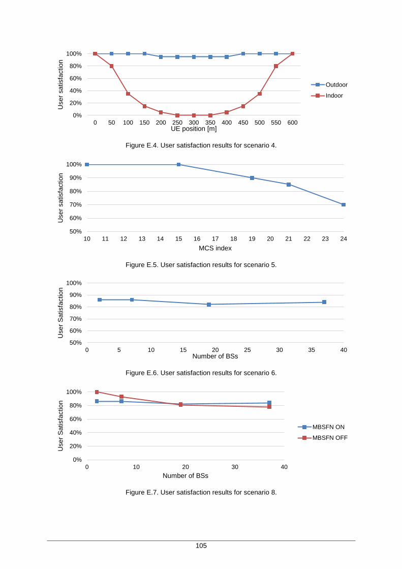
105
Figure E.4. User satisfaction results for scenario 4.
Figure E.5. User satisfaction results for scenario 5.
Figure E.6. User satisfaction results for scenario 6.
Figure E.7. User satisfaction results for scenario 8.
0%
20%
40%
60%
80%
100%
0 50 100 150 200 250 300 350 400 450 500 550 600
User
satisfa
ction
UE position [m]
Outdoor
Indoor
50%
60%
70%
80%
90%
100%
10 11 12 13 14 15 16 17 18 19 20 21 22 23 24
User
satisfa
ction
MCS index
50%
60%
70%
80%
90%
100%
0 5 10 15 20 25 30 35 40
User
Satisfa
ction
Number of BSs
0%
20%
40%
60%
80%
100%
0 10 20 30 40
User
Satisfa
ction
Number of BSs
MBSFN ON
MBSFN OFF

106
Figure E.8. User satisfaction results for Realistic Urban scenario – UEs stopped.
Figure E.9. User satisfaction results for Realistic Urban scenario – UEs moving.
Figure E.10. User satisfaction results for Realistic Rural scenario – UEs stopped.
Figure E.11. User satisfaction results for Realistic Rural scenario – UEs moving.
0%
20%
40%
60%
80%
100%
50 100 150 200 250
User
Satisfa
ction
UE-BS distance [m]
Indoor
Outdoor
0%
20%
40%
60%
80%
100%
0 20 40 60 80 100 120
User
Satisfa
ction
UE speed [km/h]
Mobility
0%
20%
40%
60%
80%
100%
0 1 2 3 4 5
User
Satisfa
ction
UE-BS distance [km]
Indoor
Outdoor
0%
20%
40%
60%
80%
100%
0 20 40 60 80 100 120
User
Satisfa
ction
UE speed [km/h]
Mobility

107
E.2 Results for comparison with the measurements
The following figures refer to the simulations made for the comparison between results from simulations
and measurements.
a) MCS index 10
b) MCS index 15
c) MCS index 19
d) MCS index 21
0 10 20 30 40 50 60 70
1
2
3
4
5
MO
S
SNR [dB]
y=1+4/(exp(12,5973-0,4567*x))R²=0,9869
0 10 20 30 40 50 60 70
1
2
3
4
5
MO
S
SNR [dB]
y=1+4/(exp(16,9691-0,6044*x))R²=0,9786
0 10 20 30 40 50 60 70
1
2
3
4
5
MO
S
SNR [dB]
y=1+4/(exp(14,7721-0,5217*x))R²=0,9916
0 10 20 30 40 50 60 70
1
2
3
4
5
MO
S
SNR [dB]
y=1+4/(exp(13,8043-0,4764*x))R²=0,9861

108
e) MCS index 24
Figure E.12. MOS vs. SNR figures, with logistic trend lines, for five different MCS indexes.
Figure E.13. MOS vs. UE-BS distance figure, with logistic trend lines, for five MCS indexes.
0 10 20 30 40 50 60 70
1
2
3
4
5
MO
S
SNR [dB]
y=1+4/(exp(11,8698-0,3904*x))R²=0,9906
1
2
3
4
5
0 100 200 300 400 500 600 700 800 900
MO
S
UE-BS distance [m]
10
15
19
21
24

109
Annex F
Additional Measurements
Results
Annex F. Additional Measurements Results
This annex presents graphs generated from the processing of the data obtained in the measurements
described in Section 4.3.

110
F.1 SINR vs. MCS index
a) MOS = 1 b) MOS = 2
c) MOS = 3 d) MOS = 4
e) MOS = 5
Figure F.1. Intervals of SINR [dB] that assures a certain MOS for each MCS index.
-10
0
10
20
30
40
10 15 19 21 24
SIN
R (
dB
)
MCS index
-10
0
10
20
30
40
10 15 19 21 24
SIN
R (
dB
)
MCS index
-10
0
10
20
30
40
10 15 19 21 24
SIN
R (
dB
)
MCS index
-10
0
10
20
30
40
10 15 19 21 24
SIN
R (
dB
)
MCS index
-10
0
10
20
30
40
10 15 19 21 24
SIN
R (
dB
)
MCS index

111
F.2 RSRP vs. MCS index
a) MOS = 1 b) MOS = 2
c) MOS = 3 d) MOS = 4
e) MOS = 5
Figure F.2. Intervals of RSRP [dBm] that assures a certain MOS for each MCS index.
-155
-145
-135
-125
-115
-105
-95
-85
-75
-65
-55
10 15 19 21 24
RS
RP
(dB
m)
MCS index
-145
-135
-125
-115
-105
-95
-85
-75
-65
-55
10 15 19 21 24
RS
RP
(dB
m)
MCS index
-145
-135
-125
-115
-105
-95
-85
-75
-65
-55
10 15 19 21 24
RS
RP
(dB
m)
MCS index
-145
-135
-125
-115
-105
-95
-85
-75
-65
-55
10 15 19 21 24
RS
RP
(dB
m)
MCS index
-145
-135
-125
-115
-105
-95
-85
-75
-65
-55
10 15 19 21 24
RS
RP
(dB
m)
MCS index

112

113
References
References
[3GPP02] 3GPP, Technical Specification Group Radio Access Network, High Speed Downlink Packet
Access: UE Radio Transmission and Reception (FDD) (Release 5), Report TR 25.890,
V1.0.0, Mar. 2002 (http://www.3gpp.org/DynaReport/25890.htm).
[3GPP06a] 3GPP, Technical Specification Group Radio Access Network, Feasibility study for evolved
Universal Terrestrial Radio Access (UTRA) and Universal Terrestrial Radio Access
Network (UTRAN) (Release 7), Report TR 25.912, V7.1.0, Oct. 2006
(http://www.3gpp.org/DynaReport/25912.htm).
[3GPP06b] 3GPP, Technical Specification Group Services and System Aspects, Policy and charging
control architecture (Release 7), Report TS 23.203, V7.1.0, Dec. 2006
(http://www.3gpp.org/DynaReport/23203.htm).
[3GPP09a] 3GPP, Technical Specification Group Services and System Aspects, Technical
Specifications and Technical Reports for an Evolved Packet System (EPS) based 3GPP
system (Release 8), Report TS 21.201, V8.1.0, Sep. 2009
(http://www.3gpp.org/DynaReport/21201.htm).
[3GPP09b] 3GPP, Technical Specification Group Radio Access Network, Evolved Universal Terrestrial
Radio Access (E-UTRA); Physical layer procedures (Release 8), Report TS 36.213, V8.8.0,
Sep. 2009 (http://www.3gpp.org/DynaReport/36213.htm).
[3GPP11a] 3GPP, Technical Specification Group Services and System Aspects, Multimedia
Broadcast/Multicast Service (MBMS); Architecture and functional description (Release 11),
Report TS 23.246, V11.0.0, Dec. 2011 (http://www.3gpp.org/DynaReport/23246.htm).
[3GPP11b] 3GPP, Technical Specification Group Radio Access Network, Spatial channel model for
Multiple Input Multiple Output (MIMO) simulations (Release 10), Report TR 25.996,
V10.0.0, Mar. 2011 (http://www.3gpp.org/DynaReport/25996.htm).
[3GPP14a] http://www.3gpp.org/technologies/keywords-acronyms/102-gprs-edge, Jan. 2014.
[3GPP14b] http://www.3gpp.org/technologies/keywords-acronyms/97-lte-advanced, Jan. 2014.
[AlcL09] Alcatel-Lucent, The LTE Network Architecture – A comprehensive tutorial, Paris, France,
2009.
[AlcL14] http://www2.alcatel-lucent.com/techzine/embms-for-more-efficient-use-of-spectrum, Jan.
2014.
[ANAC11a] ANACOM, Draft decision on the limitation of the number of rights of use of frequencies in

114
the 450 MHz, 800 MHz, 900 MHz, 1800 MHz, 2.1 GHz and 2.6 GHz bands and definition
of the respective allocation procedure, Lisbon, Portugal, Mar. 2011
(http://www.anacom.pt/render.jsp?categoryId=342072).
[ANAC11b] ANACOM, Information on multi-band spectrum auction (3), Lisbon, Portugal, Dec. 2011
(http://www.anacom.pt/render.jsp?contentId=1105917).
[ANAC13] ANACOM, Mobile Services, Statistical Information, 3rd Quarter 2013, Lisbon, Portugal, Nov.
2013 (http://www.anacom.pt/render.jsp?contentId=1182939&languageId=1).
[Anri09] Anritsu, LTE Resource Guide, 2009
(http://web.cecs.pdx.edu/~fli/class/LTE_Reource_Guide.pdf).
[Arti12] Artiza Networks, What is LTE?, 2012
(http://www.artizanetworks.com/lte_tut_what_lte.html).
[AsPe09] Assunção,P. and Pereira,F., Audiovisual Communications: Technologies, Standards and
Applications (in Portuguese), Chapter 11, IST Press, Instituto Superior Técnico, Lisbon,
Portugal, Jul. 2009.
[ASU14] http://trace.eas.asu.edu/h264/index.html, 2014.
[AT4W11] AT4 Wireless, “Overview of 3GPP releases and specifications for LTE and LTE-Advanced”,
2011.
[Cisc13] Cisco, “Cisco Visual Networking Index: Global Mobile Data Traffic Forecast Update,
2012-2017”, Feb. 2013.
[Cisc14a] http://www.cisco.com/en/US/solutions/collateral/ns341/ns973/ns1081/brochure_c02-
621881.html, Jan. 2014.
[Cisc14b] Cisco, Cisco Visual Networking Index: Global Mobile Data Traffic Forecast Update,
2013-2018, Feb. 2014
(http://www.cisco.com/en/US/solutions/collateral/ns341/ns525/ns537/ns705/ns827/white_
paper_c11-520862.html).
[Corr12] Correia,L.M., Mobile Communication Systems – Course Notes, IST-UTL, Lisbon, Portugal,
Sep. 2012.
[CoxC12] Cox,C., An introduction to LTE: LTE, LTE-advanced, SAE and 4G mobile communications,
John Wiley & Sons Ltd, Chichester, UK, 2012.
[DaFJ08] Dahlman,E., Furuskär,A., Jading,Y., Lindström,M., Parkvall,S., “Key features of the LTE
radio interface”, in Ericsson Review No. 2, 2008.
[DaPS08] Dahlman,E, Parkvall,S., Sköld,J., Beming,P., 3G Evolution: HSPA and LTE for Mobile
Broadband (2nd Edition), Elsevier Ltd., UK, 2008.
[Eric13] Ericsson, Delivering content with LTE Broadcast, Ericsson Review, Feb. 2013
(http://archive.ericsson.net/service/internet/picov/get?DocNo=28701-FGD101187).

115
[Eric14] http://www.ericsson.com/ourportfolio/telecom-operators/lte-broadcast, Feb. 2014.
[FaPe09] Faria,S. and Pereira,F., Audiovisual Communications: Technologies, Standards and
Applications (in Portuguese), Chapter 9, IST Press, Instituto Superior Técnico, Lisbon,
Portugal, Jul. 2009.
[Gonç11] Gonçalves,T., Energy efficient solutions based on beamforming for UMTS and LTE, M.Sc.
Thesis, Instituto Superior Técnico, Lisbon, Portugal, Oct. 2011.
[HaKo09] Haohong,W., Kondi,L.P., Luthra,A., Song,C., 4G Wireless Video Communications, John
Wiley & Sons Ltd., Chichester, UK, 2009.
[Hell11] Hellge,C., Skupin,R., Cho,J., Schierl,T., Wiegand,T., “Capacity improvement in EMBMS
using SVC and layer-aware bearer allocation”, Image Processing (ICIP), 2011 18th IEEE
International Conference on, Sept. 2011, pp.933-936.
[HoTo07] Holma,H. and Toskala,A., WCDMA for UMTS – HSPA Evolution and LTE (4rd Edition),
John Wiley & Sons, Chichester, UK, Nov. 2007.
[HoTo09] Holma,H. and Toskala,A., LTE for UMTS – OFDMA and SC-FDMA Based Radio Access,
John Wiley & Sons, Chichester, UK, 2009.
[ITUR09] ITU-R, Guidelines for evaluation of radio interface technologies for IMT-Advanced, Report
ITU-R M.2135-1, Dec. 2009 (http://www.itu.int/pub/R-REP-M.2135-1-2009).
[ITUR14] http://www.itu.int/net/pressoffice/press_releases/2010/48.aspx, Jan. 2014.
[ITUT07] ITU-T, Opinion model for video-telephony applications, Recommendation ITU-T G.1070,
2007 (http://www.itu.int/ITU-T/recommendations/rec.aspx?id=9050).
[ITUT08] ITU-T, Subjective video quality assessment methods for multimedia applications,
Recommendation ITU-T P.910, 2008 (https://www.itu.int/rec/T-REC-P.910-200804-I/en).
[JoAr11] Joskowicz,J., Ardao,J.C.L., “Combining the effects of frame rate, bit rate, display size and
video content in a parametric video quality model”, LANC '11 Proceedings of the 6th Latin
America Networking Conference, 2011, pp. 4-11.
[JoSo14] Joskowicz,J., Sotelo,R., “A Model for Video Quality Assessment Considering Packet Loss
for Broadcast Digital Television Coded in H.264”, International Journal of Digital Multimedia
Broadcasting, Volume 2014, Article ID 242531, Apr. 2014.
[KuOy13] Kumar,U., Oyman,O., “QoE evaluation for video streaming over eMBMS”, Computing,
Networking and Communications (ICNC), 2013 International Conference on, Jan. 2013,
pp. 555-559.
[McDo11] McDonagh,P., Vallati,C., Pande,A., Mohapatra,P., Perry,P., Mingozzi,E., “Investigation of
scalable video delivery using H.264 SVC on an LTE network”, Wireless Personal
Multimedia Communications (WPMC), 2011 14th International Symposium on, Oct. 2011,
pp. 1-5.

116
[Micr14] Microsoft, “Introduction to optimisation with the Excel Solver tool”, Sept. 2014
(http://office.microsoft.com/en-us/excel-help/introduction-to-optimisation-with-the-excel-
solver-tool-HA001124595.aspx).
[OPNE14] https://www.opnet.com/solutions/network_rd/modeler.html, May 2014.
[Remy10] Remy,J.G., “LTE-SAE: Evolution of GSM towards «All IP»”, in Computational Technologies
in Electrical and Electronics Engineering (SIBIRCON), 2010 IEEE Region 8 International
Conference on, 11-15 Jul. 2010.
[RiCh03] Ribas-Corbera,J., Chou,P.A., Regunathan,S.L., “A Generalized Hypothetical Reference
Decoder for H.264/AVC”, IEEE Transactions on Circuits and Systems for Video
Technology, Vol. 13 , Issue 7, Jul. 2003, pp. 674-687.
[Rive13] Riverbed Technology, OPNET Modeler Documentation Set, Version 17.5, 2013.
[Rive14] Riverbed Technology, Network Simulation (OPNET Modeler Suite), May 2014
(http://www.riverbed.com/products-solutions/products/network-performance-
management/network-planning-simulation/Network-Simulation.html).
[RoSc11] Rohde & Schwarz, LTE Release 9 Technology Introduction, White Paper, 2011
(http://www.rohde-schwarz.com/en/applications/lte-release-9-technology-introduction-
white-paper-application-note_56280-15541.html).
[Sams13] Samsung, eMBMS with Samsung, Simplified Approach to Broadcasting Content over LTE,
White Paper, Feb. 2013 (http://www.samsung.com/global/business/business-
images/resource/white-paper/2013/02/eMBMS-with-Samsung-0.pdf).
[Sams14] http://www.samsung.com/global/business/telecommunication-systems/news/press-
release/samsung-electronics-and-kt-join-forces-for-world-s-first-commercial-lte-embms,
Feb. 2014.
[SaPa05] Salkintzis,A.P., Passas,N., Emerging Wireless Multimedia Services and Technologies,
John Wiley & Sons Ltd., Chichester, UK, 2005.
[SeRe04] Seeling,P., Reisslein,M., Kulapala,B., “Network performance evaluation using frame size
and quality traces of single-layer and two-layer video: A tutorial”, Communications Surveys
& Tutorials Volume 6, Issue 3, IEEE, 2004.
[SeTo11] Sesia,S., Toufik,I., Baker,M., LTE – The UMTS Long Term Evolution - From Theory to
Practice, John Wiley & Sons Ltd, Chichester, UK, 2011.
[Sing12] Singh,S., Oyman,O., Papathanassiou,A., Chatterjee,D., Andrews,J.G., “Video Capacity
and QoE Enhancements over LTE”, Communications (ICC), 2012 IEEE International
Conference on, Jun. 2012, pp. 7071–7076.
[Tele14] http://www.telecompaper.com/news/zon-optimus-re-brands-as-nos--1014366, May 2014.
[Veri14] http://www.verizonwireless.com/news/article/2014/01/lte-multicast-verizon-power-
house.html, Feb. 2014.

117
[VuHu08] Vukadinovic,V., Huschke,J., “Statistical multiplexing gains of H.264/AVC video in
E-MBMS”, Wireless Pervasive Computing, 2008. ISWPC 2008. 3rd International
Symposium on, May 2008, pp. 468-474.
[WiSc03] Wiegand,T., Schwarz, H,. Joch,A., Kossentini,F., Sullivan,G.J., “Rate-Constrained Coder
Control and Comparison of Video Coding Standards”, Circuits and Systems for Video
Technology, IEEE Transactions on, Vol. 13, Issue 7, Jul. 2003, pp. 688-703.
[Yang10] Yang,X., Zhang,Y., “An Efficient SDMA Scheme Applied in Hot Spots Using Uniform
Circular Array”, in proceeding of: The IEEE International Symposium on Circuits and
Systems (ISCAS), Jan. 2010.
[Zhan09] Zhang,L., He,Z., Niu,K., Zhang,B., Skov,P., “Optimisation of Coverage and Throughput in
Single-cell eMBMS”, Vehicular Technology Conference Fall (VTC 2009-Fall), 2009 IEEE
70th, Sept. 2009, pp. 1-5.
Top Related