


Languages
Pages
Legal


2018/9/17 1
An Overview of Automatic
Speech Recognition
2018/9/17 2
Outline
1. Introduction
2. Pattern Recognition Approach
3. Two Key Technologies for ASR
4. ASR Systems and Application
5. ASR System Design Issues
6. Summary

2018/9/17 3
IntroductionSpoken language processing relies
heavily on pattern recognition (PR).
If we can incorporate the ability to PR in our work and life, we can make machines much easier to use. But the process of human PR is not well understood.
The decision for PR is based on appropriate probabilistic models of the patterns.

2018/9/17 4
Introduction
Problems of recognition
Signal variability
Environmental effects
Distinctive features are difficult to identify in continuous speech
A more successful approach
To treat the speech signal as a stochastic pattern and adopt a statistical pattern recognition

2018/9/17 5
Introduction
A source-channel speech generation
model
Speech recognition is formulated as a
maximum a posteriori decoding problem
Noisy
Channel
Channel
Decoding
Word
Sequence
Word
Sequence
Speech
Signal
Speech
Signal

2018/9/17 6
Introduction
Bayes rule
Assume speech signal S is parametrically
represented as a sequence of acoustic
vectors A
)()|()|( maxargmaxarg WPWAPAWPWW
the set of all possible sequences of words
the conditional probability of the acoustic vector sequence
the a priori probability of generating the sequence of words W

2018/9/17 7
Pattern Recognition Approach
Block diagram of a typical integrated continuous
speech recognizer
Feature
Analysis
Word
Match
Sentence
Match
Recognized
SentenceInput
Speech
Unit Model Lexicon Syntax Semantics
Language
Model
Acoustic
Word Model

2018/9/17 8
Speech Analysis and Feature
Extraction
To Parameterize speech into feature
vectors
Spectral feature
• Good discrimination
• An capability of creating statistical models
without the need for an excessive amount of
training data
• Having statistical properties which are invariant
across speakers and over a wide range of
speaking environments

2018/9/17 9
Feature Extraction Speech is a continuous evolution of the vocal tract
Need to extract time series of spectra
Use a sliding window - 16 ms window, 8 ms shift

2018/9/17 10
Speech Analysis and Feature
Extraction Implementations of feature extraction
Short-Time Spectral Features• Discrete Fourier transform(DFT)
• Linear predictive coding(LPC)
• Cepstral features with its first and second time derivatives
Frequency-Warped Spectral Features• Non-uniform frequency scales are used in
spectral analysis to provide the so-called mel-frequency spectral feature sets

2018/9/17 11
Speech Analysis and Feature
Extraction
Segment Analysis and Segment
Features
Long term analysis
Temporal decomposition
Auditory Features
Articulatory Features
Discriminative Features
Linear discriminant analysis

2018/9/17 12
Selection of Fundamental
Speech UnitsPhoneme-like units (PLUs)
The simplest set of fundamental speech units
/s/ / / /g/ /m/ / / /n/ /t/
Units other than Phones
Syllables, /seg/ /men/ /t/
Demisyllables, /s / / g/ /m / / n/ /t/
Units with Linguistic Context Dependency
triphones

2018/9/17 13
Acoustic Modeling of Speech
Units The size of training set
There is a tradeoff between using fewer subword
units(good coverage of individual units, but poor
resolution of linguistic context) and more subword
units(poor coverage of the infrequently occurring
units, but good resolution of linguistic context).
Start with some initial set of subword unit models
and adapt the models over time to the task
Hidden Markov models(HMMs)

2018/9/17 14
Lexical Modeling and Word
Level MatchLexicon
Provides a description of the words in terms of the basic set of subword units
Data-independent• Extracted from a standard dictionary and each
word in the vocabulary is represented by a single lexical entry
Data-independent• Multiple pronunciation

2018/9/17 15
Language Modeling and
Sentence Match The sentence-level matching
Grammar• Consist of a set of syntactic and semantic rules
• Can be represented as finite state network
Advance in language model Improve the efficiency and effectiveness of large
vocabulary speech recognition
Adaptive language modelingA large body of domain-specific training data
cannot be applied directly to a different task
2018/9/17 16
Search and Decision
Strategies
Finite state representation of all
knowledge source
Grammar for word sequence
The network representation of lexical
variability for words and phrases
Syllabic and phonemic knowledge used to
form fundamental linguistic units
Dynamic programming

2018/9/17 17
Two Key Technologies for
ASR
The use of HMMs modeling techniques
to characterize and model the spectral
and temporal variation of basic subword
units
The use of dynamic programming
search techniques to perform network
search

2018/9/17 18
Hidden Markov Modeling of
Speech Estimation of HMMs
Maximum likelihood• EM algorithm
• It often requires a large size training set
Maximum mutual information• Maximizes the mutual information between the given
acoustic data and the corresponding transcription
Maximum a posteriori• Adapt models to the task, to the speaker
• Bayesian learning
Minimum classification error• Minimizes the error rate on task-specific training data
• Generalized probabilistic descent(GPD)
2018/9/17 19
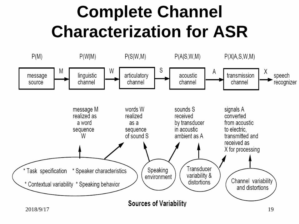
Complete Channel
Characterization for ASR

2018/9/17 20
Knowledge-Ignorant Modeling
& Channel Decoding

2018/9/17 21
LVCSR
Feature
Extraction
Subword
Models Lexicon
FeatureVectors
Word Level
Match
Recognized Sentence
Speech
Corpora
Acoustic
ModelingLanguage
ModelingText
Corpora
Speech Input
Word Model
Composition
Sentence Level
Search
Language
Models
Linguistic DecodingFront-end Processing
HMMs N-grams
Front-end Processing (前端處理) is a spectral analysis (頻譜分析)
that derives feature vectors to capture salient spectral
characteristics of speech input
Linguistic decoding (語言解碼) combines word-level matching and
sentence-level searc to perform an inverse operation to decode
the message from the speech waveform

2018/9/17 22
ASR Capabilities
Use powerful data-driven modeling tools: HMM, ANN, GM
• Rely little on detailed speech & language knowledge sources
• Give high performance in matched conditions
• Develop and deploy many applications and services
– but robustness and rigid constraints are two major limiting
factors

2018/9/17 23
Shannon’s Channel Modeling
Paradigm
Channel input is hidden (unobserved) while output is
observed and used to infer the input (which is often
approximated by a structural Markov model)
Channel modeling with (I, O) pairs in large training sets

2018/9/17 24
Modeling Input-Output
Associations Hidden Markov Model (HMM)
Artificial Neural Network (ANN)
Classification and Regression Tree (CART)
Support Vector Machine (SVM) and LVQ
Kernel-based models, mixture of experts,
Bayesian network. Graphical models, Markov random field
Many New Applications
– Rule induction, statistical parsing, machine translation
– Information retrieval, text categorization, call routing,
transliteration, pronunciation modeling, etc.

2018/9/17 25
Speech Recognition

2018/9/17 HMM and Speech Recognition 26
Hidden Markov Model - HMM

2018/9/17 HMM and Speech Recognition 27
The Markov chain
Let X=X1, X2,….Xn be a sequence of
random variables from a finite discrete
alphabet O={o1, o2,….,oM}. Based on
the Bayes’ rule
(8.1)
X are said to from a first-order Markov
chain , provided that
(8.2)
1
1 2 1 1
2
( , ,..., ) ( ) ( | )n
i
n i
i
P X X X P X P X X
1
1 1( | ) ( | )i
i i iP X X P X X

2018/9/17 HMM and Speech Recognition 28
The Markov chain
Eq.(8.1) becomes
(8.3)
Eq.(8.2) as the Markov assumption. The
Markov chain models time-invariant
(stationary) events if we discard the
time index i,
(8.4)
1 2 1 1
2
( , ,..., ) ( ) ( | )n
n i i
i
P X X X P X P X X
1( | ') ( | ')i iP X s X s P s s

HMM and Speech Recognition 29
The Markov chain
Consider a Markov chain with N distinct states {1,….,N},with the state at time t in the Markov chain denoted as st; Markov chain can be described as follows:
(8.5)
(8.6)
(8.7)
1( | ) 1 ,ij i ia P s j s i i j N
1( ) 1i P s i i N
1
1
1; 1
1
N
ij
j
N
j
j
a i N

2018/9/17 HMM and Speech Recognition 30
The Markov chain

2018/9/17 HMM and Speech Recognition 31
The Markov chain
A state-transition probability matrix of
this Dow Jones Markov chain
An initial state probability matrix
0.6 0.2 0.2
{ } 0.5 0.3 0.2
0.4 0.1 0.5
ijA a
0.5
( ) 0.2
0.3
t
i

2018/9/17 HMM and Speech Recognition 32
Markov Chain
2018/9/17 HMM and Speech Recognition 33
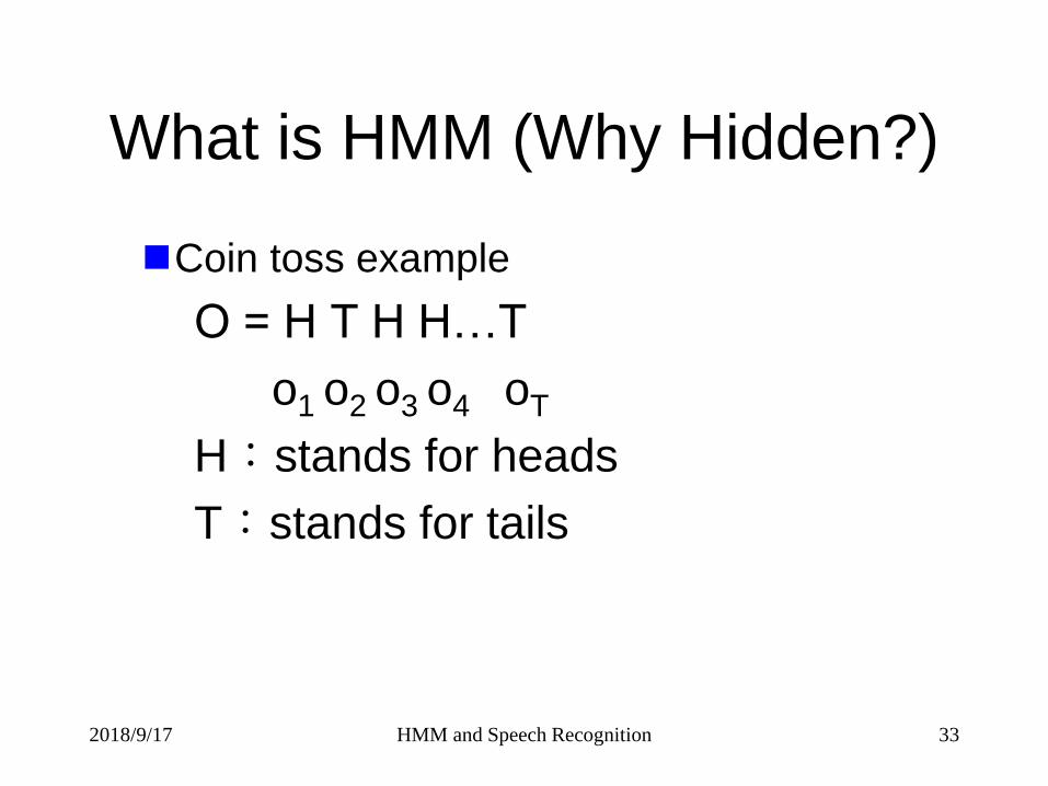
What is HMM (Why Hidden?)
Coin toss example
O = H T H H…T
o1 o2 o3 o4 oT
H:stands for heads
T:stands for tails

2018/9/17 HMM and Speech Recognition 34
1-FAIR COIN MODEL
2 states (每個state代表H or
T)
2 observation symbols
(每個symbol代表H or T)
2-FAIR COIN MODEL
2 states (每個state代表一個coin)
2 observation symbols
(每個symbol代表H or T)
Extension to Hidden Markov Model

2018/9/17 HMM and Speech Recognition 35
2-BIASED COINS MODEL
2 states
2 observation symbols
3-BIASED COINS MODEL
3 states
2 observation symbols

2018/9/17 HMM and Speech Recognition 36
How to model the outputs of the coin
tossing experiment via HMM
1. The size (the number of states) of the
model
2. The size of the observation sequence
3. Model parameters (state transition
probabilities, probabilities of heads and
tails in each state)
HMM for Coin Tossing

2018/9/17 HMM and Speech Recognition 37
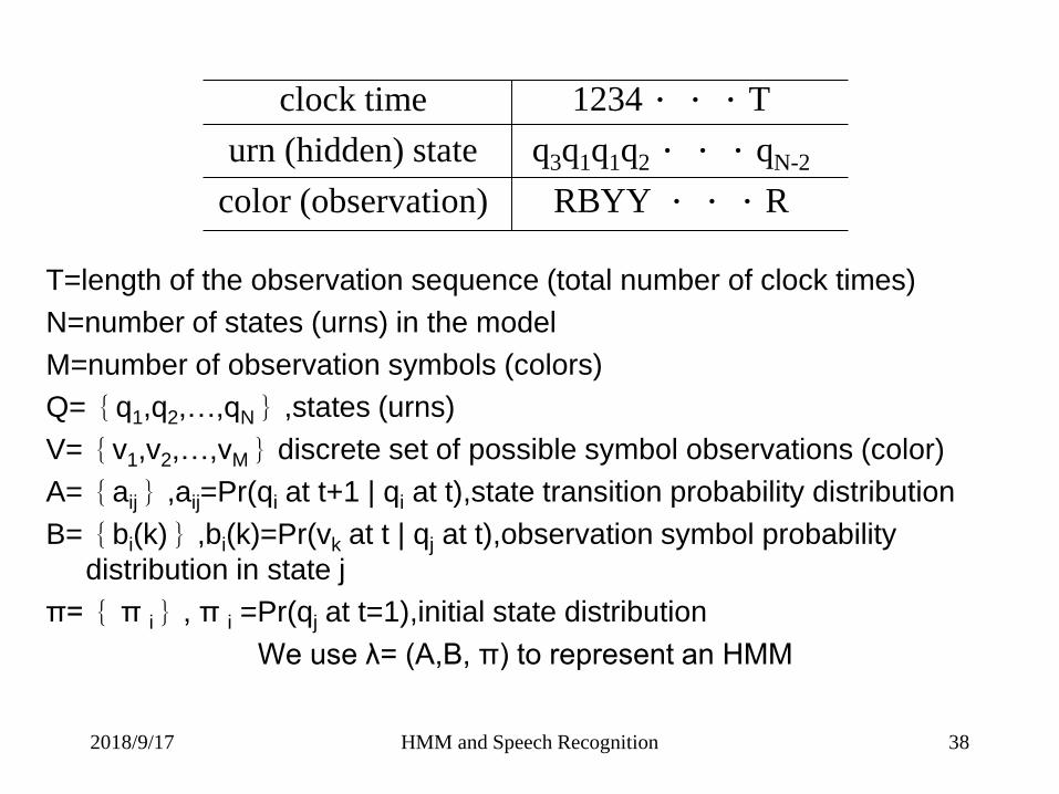
N-State Urn and Ball Model
2018/9/17 HMM and Speech Recognition 38
T=length of the observation sequence (total number of clock times)
N=number of states (urns) in the model
M=number of observation symbols (colors)
Q={q1,q2,…,qN},states (urns)
V={v1,v2,…,vM}discrete set of possible symbol observations (color)
A={aij},aij=Pr(qi at t+1 | qi at t),state transition probability distribution
B={bi(k)},bi(k)=Pr(vk at t | qj at t),observation symbol probability
distribution in state j
π={ π i}, π i =Pr(qj at t=1),initial state distribution
We use λ= (A,B, π) to represent an HMM
clock time
urn (hidden) state
color (observation)
1234...T
q3q1q1q2...qN-2
RBYY ...R

2018/9/17 HMM and Speech Recognition 39
N=4, Q={1,2,3,4} →state number
M=8, V={a,b,c,d,e,f,g,h} →observation number
T=24 →length
I=I1I2…IT →state
O=O1O2…OT →observation
ㄊ ˊ ㄞ ㄅ ˇ ㄟ
1 2 3 4
111222222223344444444444
aabcddedddcggffhffefhfff
HMM for Speech Recognition

2018/9/17 HMM and Speech Recognition 40
0.4 0.5 0.1 0
A = 0 0.6 0.3 0.1
0 0 0.6 0.4
0 0 0 1.0
a b c d e f g h
B= 0.7 0.2 0.1 0 0 0 0 0
0 0 0.2 0.6 0.2 0 0 0
0 0 0 0 0.1 0.6 0.1 0.2
π= (1,0,0,0)

2018/9/17 HMM and Speech Recognition 41
Elements of an HMM
1. There are a finite number states in the model,
say N.
2. A new state is entered based upon a
transition probability distribution which
depends on the previous state.(the Markov
property)
3. After each transition is made, an observation
output symbol is produced according to a
probability distribution which depends on the
current state.

2018/9/17 HMM and Speech Recognition 42
Basic principle
Each HMM is modeled using a set [, A, B] where
is a column matrix, A and B are square matrix.
is the initial state probability. ={i} and i, the
state index. i=1,2.. p, the HMM will have p states.
A={Aij} is the state transition probability. Aij=the
probability of moving from state i to state j.
B={Bjk} is the state observation probability. Bjk=the
observation of k pattern at state j.
2018/9/17 HMM and Speech Recognition 43
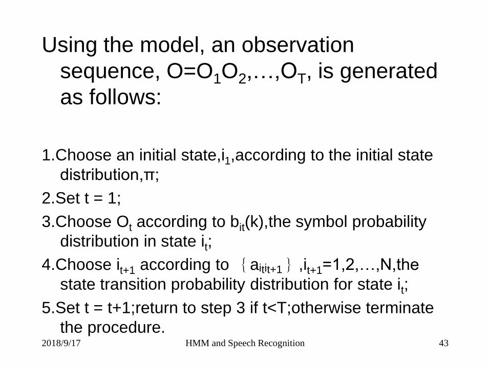
Using the model, an observation
sequence, O=O1O2,…,OT, is generated
as follows:
1.Choose an initial state,i1,according to the initial state
distribution,π;
2.Set t = 1;
3.Choose Ot according to bit(k),the symbol probability
distribution in state it;
4.Choose it+1 according to {aitit+1},it+1=1,2,…,N,the
state transition probability distribution for state it;
5.Set t = t+1;return to step 3 if t<T;otherwise terminate
the procedure.

2018/9/17 HMM and Speech Recognition 44
Three Problems for HMM
Problem1- Given the observation sequence
O=O1,O2,…,OT, and the model λ = (A,B, π),
how we compute Pr(O| λ), the probability of the
observation sequence.
Problem2- Given the observation sequence
O=O1,O2,…,OT, how we choose a state
sequence
I= i1,i2,…,iT which is optimal in some meaningful
sense.
Problem3- How we adjust the model parameters
λ= (A,B, π) to maximize Pr(O| λ).

2018/9/17 HMM and Speech Recognition 45
Solutions to the three HMM ProblemsProblem 1:
Given the model λ, the observation sequence O.
For every fixed state sequence I = i1i2…iT,
the probability of the observation sequence O is
Pr(O|I,λ)=bi1(O1) bi2(O2)... biT(OT)
The probability of such a state sequence I is
Pr(I|λ)=πi1ai1i2ai2i3… aiT-1iT
The joint probability of O and I is
Pr(O,I|λ)= Pr(O|I,λ) Pr(I|λ)
2018/9/17 HMM and Speech Recognition 46
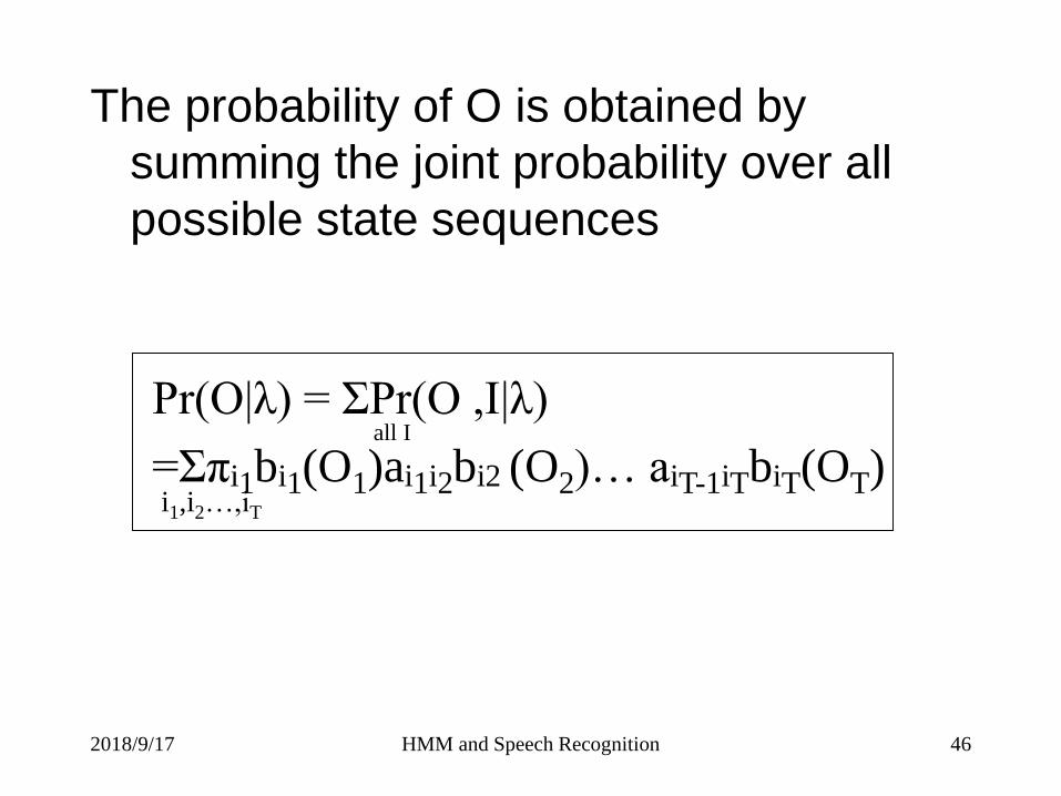
The probability of O is obtained by
summing the joint probability over all
possible state sequences
all I
i1,i2…,iT
Pr(O|λ) = ΣPr(O ,I|λ)
=Σπi1bi1(O1)ai1i2bi2 (O2)… aiT-1iTbiT(OT)

2018/9/17 HMM and Speech Recognition 47
DRAWBACK:
This method needs (2T-1)NT
multiplications and (NT -1) additions.
The calculation is on the order of 2T.NT.
If N=5, T=100, it needs 2 .100 .5100≡1072 computations!!
Clearly a more efficient procedure is
required.

2018/9/17 HMM and Speech Recognition 48
*The Forward_Backward Procedure
Def: The forward variable αt(i)
1. α1(i) = πibi(O1), 1≦i≦ N;
2. for t = 1,2,… ,T-1, 1≦j≦ N
3.then, Pr(O|λ) = Σi=1αT(i).
This method needs N(T-1)(N+1)+N multiplications and N(T-1)(N+1)+(N-1) additions. It is on the order of N2T calculations.
If N=5, T=100, it needs about 3000 computations.
αt(i) = Pr(O1, O2,… , Ot, it=qi|λ)
αt+1(j)=〔Σ αt(i)aij〕bj(Ot+1)

2018/9/17 HMM and Speech Recognition 49

2018/9/17 HMM and Speech Recognition 50

2018/9/17 HMM and Speech Recognition 51
Def : The backward variable βt(i)
1. βT(i) = 1, 1≦i ≦ N;
2, for t=T-1,T-2,… ,1, 1≦i ≦ N;
βt(i) = Σaijbj(0t+1) βt+1(j)
It requires on the order of N2T
calculations.
βt(i) = Pr(Ot+1, Ot+2,… ,OT | it = qi,λ)
βt-1(i) = Pr(OT | iT-1 = qi,λ)

2018/9/17 HMM and Speech Recognition 52
Problem 2:
*Viterbi Algorithm
Step 1-Initialization
Step 2-Recursion

2018/9/17 HMM and Speech Recognition 53
Problem 2:
*Viterbi Algorithm
Step 3-Termination
Step 4-Path (state sequence) backtracking

2018/9/17 HMM and Speech Recognition 54
Problem 3:
Def:γt(i) = Pr(it = qi | O,λ)
Def:ξt(i,j) = Pr(it = qi , it+1 = qj | O,λ)
γt(i)=αt(i)βt(i)/Pr(O| λ)
ξt(i,j) =αt(i)aijbjβt+1(j)/ Pr(O| λ)
Summing ξt(i,j) over j,giving
γt(i) = Σ ξt(i,j)N
j=1

2018/9/17 HMM and Speech Recognition 55
*Sum γt(i) & ξt(i,j) over time index t.
Σrt(j)=Expected number of times that state
qj is visited
Σt=1~T-1rt(i)=Expected number of transitions
made from qi.
Σ ξt(i,j) = Expected number of transitions
from state qi to state qj.

2018/9/17 HMM and Speech Recognition 56

2018/9/17 HMM and Speech Recognition 57
*The Baum-Welch Reestimation Formulas
1. The initial model λ defines a critical point of the
likelihood function, in which case λ= λ or
2. Model λ is more likely in the sense that
Pr(O| λ)>Pr(O| λ),i.e. we have found another
model λ, from which the observation sequence
is more likely to be produced.

2018/9/17 HMM and Speech Recognition 58
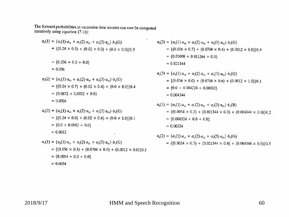
An example for HMM calcualtion
a simple 3 colored balls HMM(please go through this
sample)

2018/9/17 HMM and Speech Recognition 59
2018/9/17 HMM and Speech Recognition 60

2018/9/17 HMM and Speech Recognition 61

2018/9/17 HMM and Speech Recognition 62

2018/9/17 HMM and Speech Recognition 63
Viterbi

2018/9/17 HMM and Speech Recognition 64
Steps of ASR using HMM
Pre-emphasis
Frame blocking
Windowing
Auto-correlation analysis
LPC analysis
CEP analysis
• Codebook preparation
• HMM training
• HMM recognition
• Recognition of continuous
speech
• Post-processing

2018/9/17 HMM and Speech Recognition 65

2018/9/17 HMM and Speech Recognition 66
Pre-emphasis
The digitized signal s(n) is
put through a digital filter to
flatten the signal to make it
less susceptible to the finite
precision effects later in the
signal processing.
Common value for a is 0.95
)1()()( nsansns~

2018/9/17 HMM and Speech Recognition 67
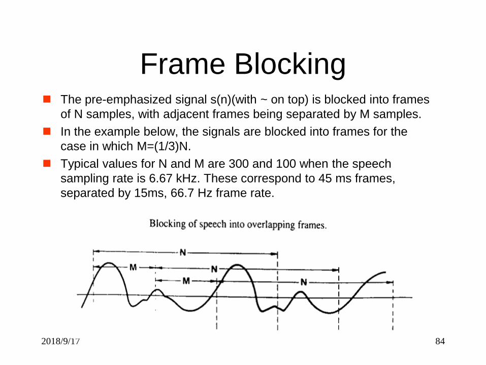
Frame Blocking The pre-emphasized signal s(n)(with ~ on top) is blocked into frames
of N samples, with adjacent frames being separated by M samples.
In the example below, the signals are blocked into frames for the
case in which M=(1/3)N.
Typical values for N and M are 300 and 100 when the speech
sampling rate is 6.67 kHz. These correspond to 45 ms frames,
separated by 15ms, 66.7 Hz frame rate.
Blocking of speech into overlapping frames.
2018/9/17 HMM and Speech Recognition 68
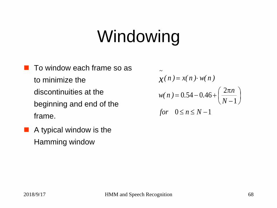
Windowing
To window each frame so as
to minimize the
discontinuities at the
beginning and end of the
frame.
A typical window is the
Hamming window
10
1
2460540
Nnfor
N
n..)n(w
)n(w)n(x)n(x~

2018/9/17 HMM and Speech Recognition 69
Auto-correlation analysis
Each frame of the
windowed signal is
auto-correlated.
Typically p is from 8 to
16.
The zeroth auto-
correlation R(0), is the
energy of the frame.
p,....,k
)kn()n()k(RkN
n
~~
xx
10
1
0

2018/9/17 HMM and Speech Recognition 70
LPC and CEP analysis
This is to convert each frame
of p+1 auto-correlation in an
LPC parameter set, which
are:
LPC coefficients
reflection coefficients
log area ratio coefficients
Read previous lectures for
details
CEP coefficients are directly
derived from LPC coefficients.
Read previous lectures for
details.
The CEP coefficients (cm) are
the coefficients of the Fourier
transform coefficients of the log
magnitude spectrum, are more
robust, reliable features se for
speech recognition than the
LPC coefficients, the reflection
coefficients and the log area
ration coefficients.
Generally, a CEP with Q>P
coefficients is used and
Q(3/2)p
refer to previous lecture

2018/9/17 HMM and Speech Recognition 71
Parameter weighting
Because of the sensitivity of
the low-order CEP to overall
spectral slope and the
sensitivity of high-order CEP
to noise, it is a standard
technique to weight the CEP
by a tapered window to
minimize these sensitivities.
A general weighting function
This function truncates the
computation and de-
emphasizes ck around k=1
and k=Q.
Qkfor
Q
ksin
Qw
cwc
k
kkk
^
1
21

2018/9/17 HMM and Speech Recognition 72
VQ = Vector Quantization
Advantages:
Reduced storage for signal
analysis
Reduced computation for
determining similarity of speech
analysis vectors.
Discretize representation of
speech sound. By associating a
phonetic label with each
codebook vector, the process of
choosing a best codebook
vector to represent a give
speech vector becomes
equivalent to assigning a
phonetic label to each speech
frame.
Disadvantages
an inherent signal distortion in
representing the actual speech
vector
the storage required for
codebook vector is nontrivial.
There will be trade-off among
quantization error, processing
time and storage.
2018/9/17 HMM and Speech Recognition 73
2018/9/17 HMM and Speech Recognition 74
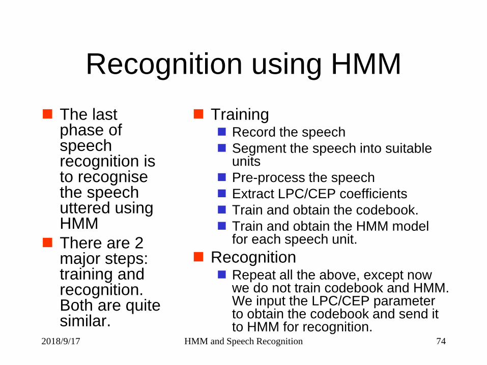
Recognition using HMM
The last phase of speech recognition is to recognise the speech uttered using HMM
There are 2 major steps: training and recognition. Both are quite similar.
Training Record the speech
Segment the speech into suitable units
Pre-process the speech
Extract LPC/CEP coefficients
Train and obtain the codebook.
Train and obtain the HMM model for each speech unit.
Recognition Repeat all the above, except now
we do not train codebook and HMM. We input the LPC/CEP parameter to obtain the codebook and send it to HMM for recognition.

2018/9/17 HMM and Speech Recognition 75
Recognition of Continuous
Words
Three methods
Two-level dynamic programming
Level Builing algorithm
One-pass algorithm
• details in L Rabiner and B H Juang, Chapter 7
2018/9/17 HMM and Speech Recognition 76
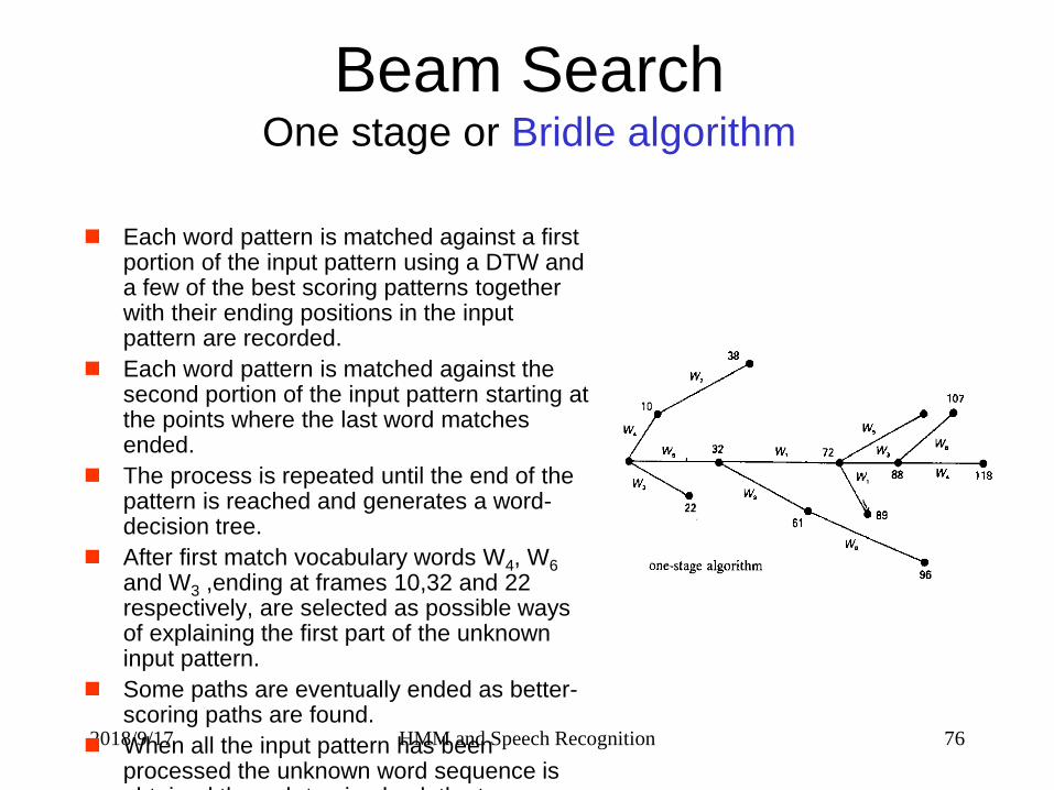
Beam SearchOne stage or Bridle algorithm
Each word pattern is matched against a first portion of the input pattern using a DTW and a few of the best scoring patterns together with their ending positions in the input pattern are recorded.
Each word pattern is matched against the second portion of the input pattern starting at the points where the last word matches ended.
The process is repeated until the end of the pattern is reached and generates a word-decision tree.
After first match vocabulary words W4, W6
and W3 ,ending at frames 10,32 and 22 respectively, are selected as possible ways of explaining the first part of the unknown input pattern.
Some paths are eventually ended as better-scoring paths are found.
When all the input pattern has been processed the unknown word sequence is obtained through tracing back the tree.

2018/9/17 HMM and Speech Recognition 77
Post-processing
Post-processing increase the recognition rate
significantly(reducing the error rate to 1/2 or
1/3)
Post-processing techniques
N-gram
Grammar, syntactical parsers such as PCFG, Link
Grammar
Semantic parsers (Logic parser?)
Trigger pairs - long distance dependency
Many other ….

2018/9/17 HMM and Speech Recognition 78
HMM - Hidden Markov Model
Three types:
discrete DHMM(poor performance)
continuous CHMM(require huge speech
data for training)
semi-continuous SCHMM(best)

2018/9/17 HMM and Speech Recognition 79
*HMM on Speech Recognition

2018/9/17 HMM and Speech Recognition 80
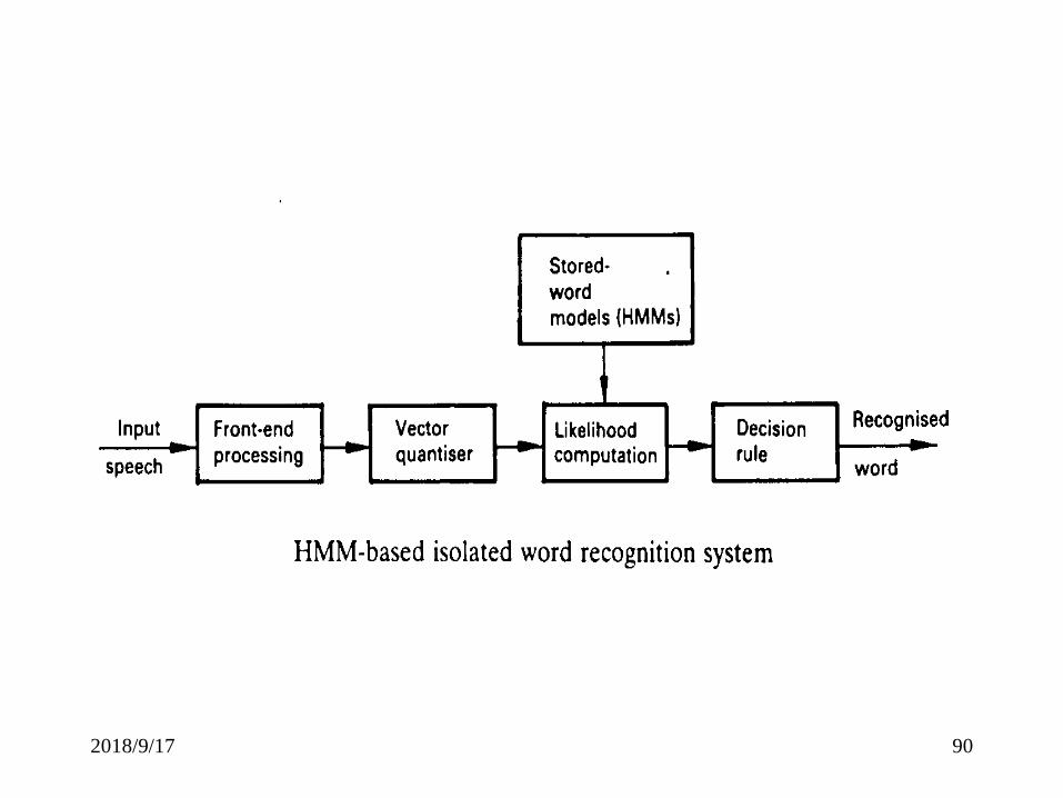
Example: Isolated Word Recognition
Assume we have a vocabulary of V words to be
recognized. We have a training set of L tokens
of each word (spoken by 1 or more talkers).
1. Build an HMM for each word in the vocabulary
λk,1≦k ≦ V
2. For each unknown word, characterized by
observation sequence 0=01, 02, 03,…, 0T
3. Scoring procedure
For each word model, λk,calculate Pk=Pr(0| λk)
4. Choose the word whose model probability is
highest.

2018/9/17 81
Steps of ASR using HMM
Pre-emphasis
Frame blocking
Windowing
Auto-correlation analysis
LPC analysis
CEP analysis
Codebook preparation
HMM training
HMM recognition
Recognition of continuous
speech
Post-processing

2018/9/17 82

2018/9/17 83
Pre-emphasis
The digitized signal s(n) is put through a
digital filter to flatten the signal to make
it less susceptible to the finite precision
effects later in the signal processing.
Common value for a is 0.95
)1()()( nsansns~
2018/9/17 84
Frame Blocking The pre-emphasized signal s(n)(with ~ on top) is blocked into frames
of N samples, with adjacent frames being separated by M samples.
In the example below, the signals are blocked into frames for the
case in which M=(1/3)N.
Typical values for N and M are 300 and 100 when the speech
sampling rate is 6.67 kHz. These correspond to 45 ms frames,
separated by 15ms, 66.7 Hz frame rate.

2018/9/17 85
Windowing
To window each frame so as to minimize the
discontinuities at the beginning and end of the
frame.
A typical window is the Hamming window
10
1
2460540
Nnfor
N
n..)n(w
)n(w)n(x)n(x~

2018/9/17 86
Auto-correlation analysis
Each frame of the windowed signal is auto-
correlated.
Typically p is from 8 to 16.
The zeroth auto-correlation R(0), is the
energy of the frame.
p,....,k
)kn()n()k(RkN
n
~~
xx
10
1
0

2018/9/17 87
LPC and CEP analysis This is to convert each frame of p+1 auto-correlation in an
LPC parameter set, which are: LPC coefficients
reflection coefficients
log area ratio coefficients
CEP coefficients are directly derived from LPC coefficients. Read previous lectures for details.
The CEP coefficients (cm) are the coefficients of the Fourier transform coefficients of the log magnitude spectrum, are more robust, reliable features se for speech recognition than the LPC coefficients, the reflection coefficients and the log area ration coefficients.
Generally, a CEP with Q>P coefficients is used and Q(3/2)p refer to previous lecture

2018/9/17 88
Parameter weighting
Because of the sensitivity of the low-order CEP to overall
spectral slope and the sensitivity of high-order CEP to
noise, it is a standard technique to weight the CEP by a
tapered window to minimize these sensitivities.
A general weighting function
This function truncates the computation and de-emphasizes ck
around k=1 and k=Q.
Qkfor
Q
ksin
Qw
cwc
k
kkk
^
1
21

2018/9/17 89
VQ = Vector Quantization
Advantages:
Reduced storage for signal
analysis
Reduced computation for
determining similarity of speech
analysis vectors.
Discretize representation of
speech sound. By associating a
phonetic label with each
codebook vector, the process of
choosing a best codebook
vector to represent a give
speech vector becomes
equivalent to assigning a
phonetic label to each speech
frame.
Disadvantages
an inherent signal distortion in
representing the actual speech
vector
the storage required for
codebook vector is nontrivial.
There will be trade-off among
quantization error, processing
time and storage.
2018/9/17 90

2018/9/17 91
Recognition using HMM
The last phase of speech recognition is to recognise the speech uttered using HMM
There are 2 major steps: training and recognition. Training
• Record the speech
• Segment the speech into suitable units
• Pre-process the speech
• Extract LPC/CEP coefficients
• Train and obtain the codebook.
• Train and obtain the HMM model for each speech unit.
Recognition
• Repeat all the above, except now we do not train codebook and HMM. We input the LPC/CEP parameter to obtain the codebook and send it to HMM for recognition.

2018/9/17 92
Recognition of Continuous
Words
Three methods
Two-level dynamic programming
Level Builing algorithm
One-pass algorithm
• details in L Rabiner and B H Juang, Chapter 7

2018/9/17 93
Beam SearchOne stage or Bridle algorithm
Each word pattern is matched against a first portion of the input pattern using a DTW and a few of the best scoring patterns together with their ending positions in the input pattern are recorded.
Each word pattern is matched against the second portion of the input pattern starting at the points where the last word matches ended.
The process is repeated until the end of the pattern is reached and generates a word-decision tree.
After first match vocabulary words W4, W6 and W3 ,ending at frames 10,32 and 22 respectively, are selected as possible ways of explaining the first part of the unknown input pattern.
Some paths are eventually ended as
better-scoring paths are found.
When all the input pattern has been processed
the unknown word sequence is obtained
through tracing back the tree.

2018/9/17 94
Post-processing
Post-processing increase the recognition rate
significantly(reducing the error rate to 1/2 or
1/3)
Post-processing techniques
N-gram
Grammar, syntactical parsers such as PCFG, Link
Grammar
Semantic parsers (Logic parser?)
Trigger pairs - long distance dependency
Many other ….

2018/9/17 95
HMM - Hidden Markov Model
Three types:
discrete DHMM(poor performance)
continuous CHMM(require huge speech
data for training)
semi-continuous SCHMM(best)

2018/9/17 96
*HMM on Speech Recognition

2018/9/17 97
Example: Isolated Word Recognition
Assume we have a vocabulary of V words to be
recognized. We have a training set of L tokens
of each word (spoken by 1 or more talkers).
1. Build an HMM for each word in the vocabulary
λk,1≦k ≦ V
2. For each unknown word, characterized by
observation sequence 0=01, 02, 03,…, 0T
3. Scoring procedure
For each word model, λk,calculate Pk=Pr(0| λk)
4. Choose the word whose model probability is
highest.

2018/9/17 98
4. Speech Recognition
Application Telecommunications
Providing information or access to data or service over telephone lines
Office / desktopVoice control of PC
Voice control of telephony functionality
Manufacturing and business
Medical / legalCreate various reports and forms
Other applicationsUsing speech recognition in toys and games

2018/9/17 99
5. ASR System Design Issues
Signal capturing and noise reduction
Microphone array
Acoustic variability and robustness issues
Database collection limitation
Static versus dynamic system design
Spontaneous speech and keyword spotting
Human factors issues

2018/9/17 100
6. Summary
Research Challenges Robust speech recognition to improve the usability
of a system in a wide variety of speaking condition for a large population of speakers
Robust utterance verification to relax the rigid speaking format and to be able to extract relevant partial information in spontaneous speech and attach a recognition confidence to it
High performance speech recognition through adaptive system design to quickly meet changing tasks, speakers and speaking environments
Top Related