


Languages
Pages
Legal


Copyright © James W. Kamman, 2016
An Introduction to
Three-Dimensional, Rigid Body Dynamics
James W. Kamman, PhD
Volume II: Kinetics
Unit 3
Degrees of Freedom, Partial Velocities and Generalized Forces
Summary
This unit defines the concepts of degrees of freedom, generalized coordinates, partial velocities, partial
angular velocities and generalized forces. These concepts form an introduction to methods of treating
systems with multiple bodies as systems rather than one body at a time as with the Newton/Euler equations
of motion.
Page Count Examples Suggested Exercises
18 7 6

Copyright © James W. Kamman, 2016 Volume II, Unit 3: page 1/18
Degrees of Freedom of Mechanical Systems
System Configuration and Generalized Coordinates
The configuration of a mechanical system is defined as the position of
each of the bodies within the system at a particular instant. In general,
both translational and rotational coordinates are needed to describe the
position of a rigid body. Together the translation and rotation coordinates
are called generalized coordinates. For the simple pendulum shown, Gx
and Gy are translational coordinates that describe the location of the
mass center of the bar, and is a rotational coordinate that describes the
orientation of the bar.
Typically, the generalized coordinates used to define the configuration of the mechanical system form a
dependent set. That is, the coordinates are not independent of each other. For example, for the simple
pendulum Gx , Gy , and are not independent, because the following two independent constraint equations
can be written
12
sin ( )G
x L 12
cos ( )G
y L
Given the value of one of the coordinates, these equations can be used to compute the values of the other two
coordinates, so only one of the coordinates is needed. Any pair of these coordinates forms a dependent set.
Note:
Generalized coordinates need not always directly represent translational or rotational variables, but
they will for the purpose of this text.
Generalized Coordinates and Degrees of Freedom
The number of degrees of freedom (DOF) of a
mechanical system is defined as the minimum number of
generalized coordinates necessary to define the
configuration of the system. For a set of generalized
coordinates to be minimum in number, the coordinates must
form an independent set. The figures to the right show
examples of one, two, and three degree-of-freedom planar
systems.
For mechanical systems that consist of a series of
interconnected bodies, it may not be obvious how many
Simple Pendulum
Copyright © James W. Kamman, 2016 Volume II, Unit 3: page 2/18
degrees of freedom the system possesses. For these systems,
the number of degrees of freedom can be found by first
calculating the number of degrees of freedom the system
would possess if the motions of all the bodies were
unrestricted and then subtracting the total number of
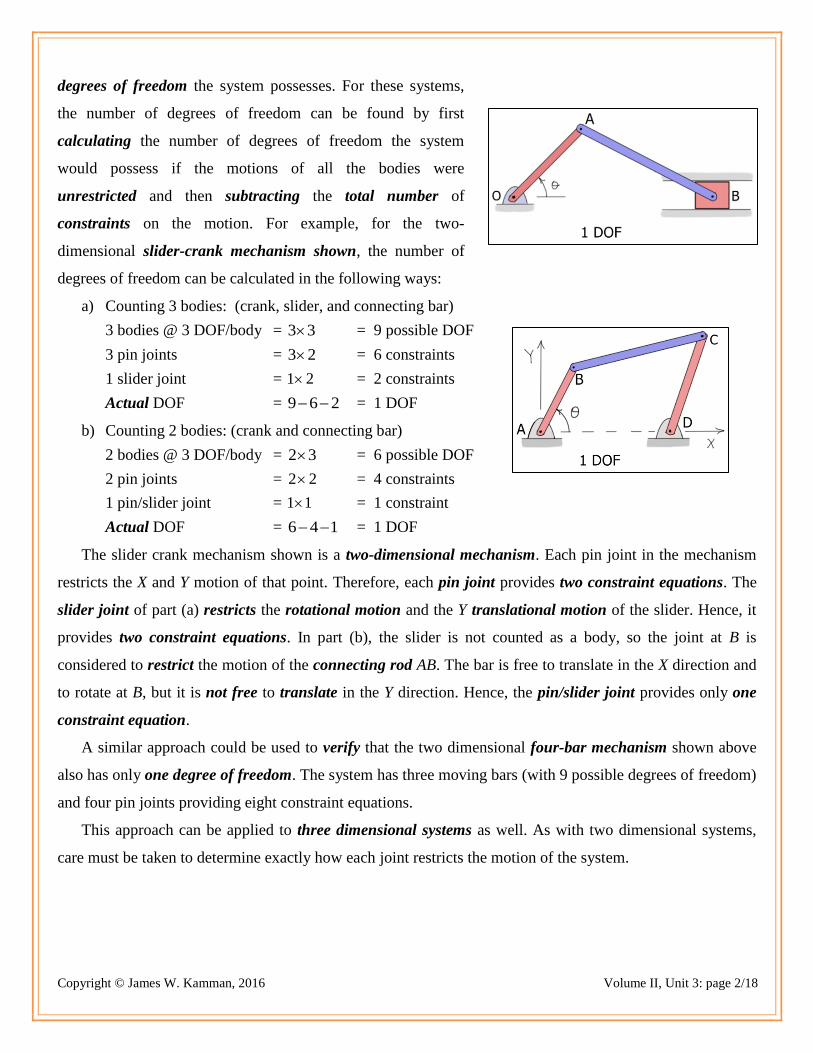
constraints on the motion. For example, for the two-
dimensional slider-crank mechanism shown, the number of
degrees of freedom can be calculated in the following ways:
a) Counting 3 bodies: (crank, slider, and connecting bar)
3 bodies @ 3 DOF/body = 3 3 = 9 possible DOF
3 pin joints = 3 2 = 6 constraints
1 slider joint = 1 2 = 2 constraints
Actual DOF = 9 6 2 = 1 DOF
b) Counting 2 bodies: (crank and connecting bar)
2 bodies @ 3 DOF/body = 2 3 = 6 possible DOF
2 pin joints = 2 2 = 4 constraints
1 pin/slider joint = 1 1 = 1 constraint
Actual DOF = 6 4 1 = 1 DOF
The slider crank mechanism shown is a two-dimensional mechanism. Each pin joint in the mechanism
restricts the X and Y motion of that point. Therefore, each pin joint provides two constraint equations. The
slider joint of part (a) restricts the rotational motion and the Y translational motion of the slider. Hence, it
provides two constraint equations. In part (b), the slider is not counted as a body, so the joint at B is
considered to restrict the motion of the connecting rod AB. The bar is free to translate in the X direction and
to rotate at B, but it is not free to translate in the Y direction. Hence, the pin/slider joint provides only one
constraint equation.
A similar approach could be used to verify that the two dimensional four-bar mechanism shown above
also has only one degree of freedom. The system has three moving bars (with 9 possible degrees of freedom)
and four pin joints providing eight constraint equations.
This approach can be applied to three dimensional systems as well. As with two dimensional systems,
care must be taken to determine exactly how each joint restricts the motion of the system.
Copyright © James W. Kamman, 2016 Volume II, Unit 3: page 3/18
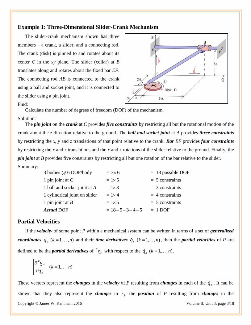
Example 1: Three-Dimensional Slider-Crank Mechanism
The slider-crank mechanism shown has three
members – a crank, a slider, and a connecting rod.
The crank (disk) is pinned to and rotates about its
center C in the xy plane. The slider (collar) at B
translates along and rotates about the fixed bar EF.
The connecting rod AB is connected to the crank
using a ball and socket joint, and it is connected to
the slider using a pin joint.
Find:
Calculate the number of degrees of freedom (DOF) of the mechanism.
Solution:
The pin joint on the crank at C provides five constraints by restricting all but the rotational motion of the
crank about the z direction relative to the ground. The ball and socket joint at A provides three constraints
by restricting the x, y and z translations of that point relative to the crank. Bar EF provides four constraints
by restricting the x and z translations and the x and z rotations of the slider relative to the ground. Finally, the
pin joint at B provides five constraints by restricting all but one rotation of the bar relative to the slider.
Summary:
3 bodies @ 6 DOF/body = 3 6 = 18 possible DOF
1 pin joint at C = 1 5 = 5 constraints
1 ball and socket joint at A = 1 3 = 3 constraints
1 cylindrical joint on slider = 1 4 = 4 constraints
1 pin joint at B = 1 5 = 5 constraints
Actual DOF = 18 5 3 4 5 = 1 DOF
Partial Velocities
If the velocity of some point P within a mechanical system can be written in terms of a set of generalized
coordinates ( 1, , )kq k n and their time derivatives ( 1, , )kq k n , then the partial velocities of P are
defined to be the partial derivatives of R
Pv with respect to the ( 1, , )kq k n .
( 1, , )
R
P
k
vk n
q
These vectors represent the changes in the velocity of P resulting from changes in each of the kq . It can be
shown that they also represent the changes in Pr the position of P resulting from changes in the

Copyright © James W. Kamman, 2016 Volume II, Unit 3: page 4/18
( 1, , )kq k n . They are a measure of the sensitivity of the velocity (or position) of P to changes in the kq
(or kq ). In this regard, they can also provide a measure of the mechanical advantage or disadvantage
associated with changes in any of the generalized coordinates. If small changes in the generalized
coordinates produce large changes in the position of P, then the provider has a mechanical disadvantage. If
large changes in the generalized coordinates produce small changes in the position of P, then the provider
has a mechanical advantage.
From the perspective of multivariate calculus, if the position vector of P is a function of the generalized
coordinates and time, that is, ( , )P P kr r q t , then R
Pv the velocity of P can be written as follows.
1
R nP P PR
P k
k k
dr r rv q
dt q t
From this result, it also follows that
R
P P
k k
v r
q q
The term Pr
t
accounts for position vectors that depend explicitly on time (e.g. some specified motion).
Note that since the velocity is linear in the ( 1, , )kq k n , the partial velocities are found by
inspection of the velocity vector.
Partial Angular Velocities
Similarly, if the angular velocity of a body B within a mechanical system can be written in terms of a set
of generalized coordinates ( 1, , )kq k n and their time derivatives ( 1, , )kq k n , then the partial
angular velocities of B are defined to be the partial derivatives of R
B with respect to the ( 1, , )kq k n .
( 1, , )
R
B
k
k nq
These vectors represent changes in the angular velocity of a body resulting from changes in the
( 1, , )kq k n . In general, the angular velocity can be written in terms of the partial angular velocities as
1
( )
RnBR R
B k B t
k k
where ( )R
B t is that part of the angular velocity vector that depends explicitly on time.
Copyright © James W. Kamman, 2016 Volume II, Unit 3: page 5/18
Note the above equation cannot generally be formulated using a differentiation process as there is no
vector whose derivative is the angular velocity. The angular velocity is formed using the summation rule for
angular velocities, and as with the partial velocities, the partial angular velocities are found by inspection.
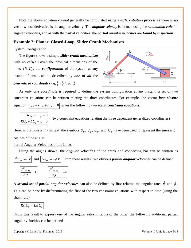
Example 2: Planar, Closed-Loop, Slider Crank Mechanism
System Configuration
The figure shows a simple slider crank mechanism
with no offset. Given the physical dimensions of the
links ( , )R L , the configuration of the system at any
instant of time can be described by one or all the
generalized coordinates , ,kq x .
As only one coordinate is required to define the system configuration at any instant, a set of two
constraint equations can be written relating the three coordinates. For example, the vector loop-closure
equation / / / 0B A C B A Cr r r gives the following two scalar constraint equations.
0
0
RS LS
RC LC x
(two constraint equations relating the three dependent generalized coordinates)
Here, as previously in this text, the symbols S , S , C and C have been used to represent the sines and
cosines of the angles.
Partial Angular Velocities of the Links
Using the angles shown, the angular velocities of the crank and connecting bar can be written as
R
AB k and R
BC k . From these results, two obvious partial angular velocities can be defined.
R
ABk
R
BCk
A second set of partial angular velocities can also be defined by first relating the angular rates and .
This can be done by differentiating the first of the two constraint equations with respect to time (using the
chain rule).
R C L C
Using this result to express one of the angular rates in terms of the other, the following additional partial
angular velocities can be defined
Copyright © James W. Kamman, 2016 Volume II, Unit 3: page 6/18
R
BC RC RCk k k
LC LC
R
ABLC LC
k k kRC RC
Note that
R
BC
becomes zero when the crank angle 90 (deg) . In this position, the connecting rod BC
is translating and not rotating, so changing the angular velocity of the crank has no effect on the angular
velocity of the connecting rod. Conversely, R
AB
becomes undefined when the crank angle 90 (deg) .
Near this position, the angular velocity of the crank is very sensitive to changes in the angular velocity of the
connecting rod.
Partial Velocities of the Slider
The velocity of the slider can be written most simply as R
Cv x i . From this result, the following partial
velocity can be defined
R
Cvi
x
Additional partial velocities can be defined by relating x to the angular rates and . This can be done by
differentiating the second of the constraint equations with respect to time and using the chain rule.
x R S L S
Using this result, R
Cv the velocity of the slider can be written as
R
Cv x i R S L S i
Using this result and the equation above relating the angular rates and , the following additional partial
velocities can be defined.
R
C
RCv RS L S i
L C
R
CvR S C S C i
R
C
LCv R S LS i
R C
R
CvL S C S C i
Note when the crank angle 0 (or 180) (deg) , both of these partial velocities are zero, but when
90 (deg) , Cv
R i
and
Cv
is undefined. Recall that when 0 (or 180) (deg) , the velocity of

Copyright © James W. Kamman, 2016 Volume II, Unit 3: page 7/18
the slider is zero and both bars are rotating about their end points, and when 90 (deg) the connecting
rod is translating. When the connecting rod is translating, the crank angular velocity has its largest influence
on the velocity of the slider.
Example 3: Six DOF Arm
The system shown is a six DOF double pendulum or
arm. The first link is connected to ground and the second
link is connected to the first with ball and socket joints at O
and A. The ground frame is 1 2 3: , ,R N N N and the link
frames are 1 2 3: , , ( 1, 2)ii i iL n n n i . The orientation of
each link is defined relative to R using a 3-1-3 body-fixed
rotation sequence. The lengths of the links are 1 and 2 .
Find:
a) Partial angular velocities of the links associated with the rates of the six orientation angles.
b) Partial velocities of point B associated with the rates of the six orientation angles.
Solution:
Previous results:
In Unit 7 of Volume I the angular velocities of the links and the velocity of B were found to be
1 1 2 2 3 3i
R i i i
L i i in n n with
1 1 2 3 2 3
2 1 2 3 2 3
3 3 1 2
i i i i i i
i i i i i i
i i i i
S S C
S C S
C
( 1,2)i
1 1 2 21 13 1 1 11 3 2 23 1 2 21 3
RBv n n n n
a) Using these results, the following partial angular velocities can be identified.
1 1 1 1
12 13 1 12 13 2 12 3
11
R
LS S n S C n C n
1 1 1
13 1 13 2
12
R
LC n S n
1 1
3
13
R
Ln
2 2 2 2
22 23 1 22 23 2 22 3
21
R
LS S n S C n C n
2 2 2
23 1 23 2
22
R
LC n S n
2 2
3
23
R
Ln
b) The following partial velocities can also be identified.

Copyright © James W. Kamman, 2016 Volume II, Unit 3: page 8/18
1 1
1 12 1 1 12 13 3
11
R
BvC n S S n
1
1 13 3
12
R
BvC n
1
1 1
13
R
Bvn
2 2
2 22 1 2 22 23 3
21
R
BvC n S S n
2
2 23 3
22
R
BvC n
2
2 1
23
R
Bvn
Recall that matrices 1
T
R and 2
T
R transform the link-based components into the base frame. Hence, the
results shown for the partial velocities and partial angular velocities could all be easily transformed into the
base frame using the transformation matrices.
Generalized Forces
Given a mechanical system whose configuration is defined by a set of generalized coordinates
( 1,..., )kq k n , the generalized forces associated with each of the “n” generalized coordinates as
( ) ( )
k
RRji
q i j
forces torquesk ki j
vF F M
q q
( 1, , )k n
Here the index “i” represents each of the forces, the index “j” represents each of the torques, and the index
“k” represents each of the generalized coordinates. The forces iF and the torques
jM that have non-zero
contributions to this sum are said to be active.
Conservative and Nonconservative Forces
Consider a particle that moves from position 1 to position 2
along one path (forward path) and back again to position 1
along a second path (return path) as shown in the diagram. A
force acting on the particle is said to be conservative if the net
work it does over the closed path is zero. Suppose, for
example, that the work done by the force as the particle moves
from position 1 to position 2 is positive, then the force does the
same amount of work as the particle returns to position 1,
except that this work is negative.
In this way, conservative forces do not permanently add or remove energy from a system. When the
conservative force is doing negative work, the system is said to be gaining potential energy that can later be
transformed into kinetic energy. It is also true of conservative forces that the work done in moving from one
position to another is independent of the path of the particle. Examples include weight forces and spring
forces and torques.

Copyright © James W. Kamman, 2016 Volume II, Unit 3: page 9/18
Forces whose net work around a closed circuit is not zero are called nonconservative forces. The work
done by these forces as a particle moves from one position to another is dependent on the path of the
particle. Examples include friction and damping forces and torques.
Conservative Forces and Potential Energy (V)
The generalized force associated with conservative forces and torques can be written in terms of a
potential energy function, V. For weight forces and linear spring forces and torques, the potential energy
functions are
V W y mg y ( y is the height of the particle above some arbitrary datum)
212
V ke ( e is the elongation or compression of the spring (units of length))
212
V k ( is the elongation or compression of the spring (radians or degrees))
For systems with multiple conservative forces, the system potential energy is i
i
V V .
If conservative forces and torques do work on a system (i.e. if they are active), their contribution to the
generalized forces can be calculated using the definition given above or they can be calculated using the
potential energy function V .
kq
k
VF
q
( 1, , )k n
Viscous Damping and Rayleigh’s Dissipation Function (R)
One type of nonconservative force or torque is associated with viscous damping. One way of modeling
this phenomenon is to assume that the forces or torques are proportional to the relative velocity or relative
angular velocity of the end points of the element.
Force: relF cv Torque: relM c n
Here, the direction of the unit vector n is defined by the right-hand rule. For these types of nonconservative
forces and torques, Rayleigh’s dissipation function is
Force: 2
rel12
R c x Torque: 2
rel12
R c
Here, the symbols relx and rel have been used to represent the rates of translational and rotational motion
between the ends of the damping element. For systems with multiple proportional damping elements, the
system dissipation function is i
i
R R .

Copyright © James W. Kamman, 2016 Volume II, Unit 3: page 10/18
The contribution of these forces and/or torques to the generalized forces can be calculated using the
definition given above or they can be calculated using Rayleigh’s dissipation function.
kq
k
RF
q
( 1, , )k n
Example 4: Planar, One-Link Pendulum
The one link pendulum shown is acted upon by gravity and by the
applied moment M. The Y axis is pointed in the direction of gravity. The
single coordinate describes the position of the pendulum.
Find:
F , the generalized force associated with the coordinate
Solution:
The mechanical system in this case is a single body – the pendulum
link. Using the general definition of the generalized force acting on the
system associated with the coordinate is defined to be
( ) ( ) zero
R R RR Ri O Gj
i j O
forces torquesi j
v v vF F M F W M
The angular velocity of the bar, the velocity of the mass center G can be written as follows.
RB k 1 1 1
2 2 2
RR
G
dv LS i LC j L C i S j
dt
Substituting into the generalized force equation gives
1 12 2
R RGv
F W M W j L C i S j M k k W LS M
Note:
The contribution of the weight force could have been calculated using the potential energy function for
gravity. Assuming a horizontal datum along the X axis passing through O
1 12 2W
F W LC W LS

Copyright © James W. Kamman, 2016 Volume II, Unit 3: page 11/18
Example 5: Loaded, Planar, Slider-Crank Mechanism
The figure shows a slider crank mechanism under
the action of an external torque T acting on link AB,
external forces P and Q acting at B and C, and a linear
spring attached at B. The spring has stiffness k, an
unstretched length of u , and it always remains
horizontal. Neglect weight forces and friction.
Find:
F the generalized force associated with the coordinate
Solution:
The system in this case is the entire slider-crank mechanism. The active forces and torques acting on
the system are the forces P and Q, the torque T, and the linear spring force. The pin forces at A, B and C and
the wall force on the slider are not active. Why? The pin at A has zero velocity and zero partial velocity. The
pin at B has nonzero velocity and partial velocity, but the internal forces on members AB and BC are equal
and opposite, so their net contribution is zero. The same is true for the pin forces at C acting on the BC and
the slider. Without friction, the wall force is perpendicular to the velocity of C, and hence it is not active. So,
the generalized force F can be written as follows.
spring
( ) ( )
R R
i j
i j P Q Tforces torques
i j
R R R R
B C AB B
s
vF F M F F F F
v v vP i Q i T k F i
The angular velocity of AB and the velocity of B can be written as
R
AB k /R R
B B Av v k R C i S j R S i C j
The velocity of C was found in Example 2 to be
R
Cv R S C S C i
Substituting these results into the definition of F gives
R R R R
B C AB B
s
s
v v vF P i Q i T k F i
P F i R S i C j Q i R S C S C i T k k
Copyright © James W. Kamman, 2016 Volume II, Unit 3: page 12/18
sF F P RS QR S C S C T
The spring force is equal to the product of the spring stiffness and elongation, or s uF k RC . The
contribution of the spring force to F can also be calculated using the potential energy function of the
spring. Specifically,
2spring
spring
12 u u u
VF k RC k RC RS kRS RC
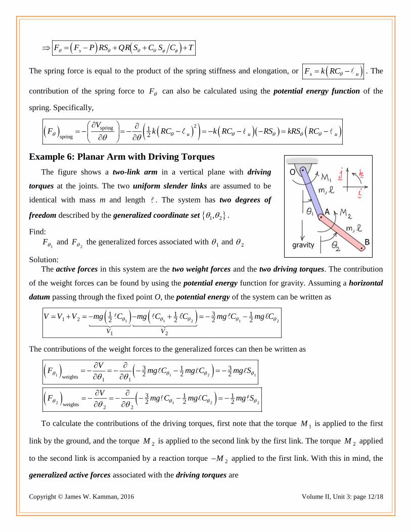
Example 6: Planar Arm with Driving Torques
The figure shows a two-link arm in a vertical plane with driving
torques at the joints. The two uniform slender links are assumed to be
identical with mass m and length . The system has two degrees of
freedom described by the generalized coordinate set 1 2, .
Find:
1
F and 2
F the generalized forces associated with 1 and 2
Solution:
The active forces in this system are the two weight forces and the two driving torques. The contribution
of the weight forces can be found by using the potential energy function for gravity. Assuming a horizontal
datum passing through the fixed point O, the potential energy of the system can be written as
1 1 2 1 21 2
1 2
31 1 12 2 2 2
V V
V V V mg C mg C C mg C mg C
The contributions of the weight forces to the generalized forces can then be written as
1 1 2 1weights1 1
3 312 2 2
VF mg C mg C mg S
2 1 2 2weights2 2
3 1 12 2 2
VF mg C mg C mg S
To calculate the contributions of the driving torques, first note that the torque 1M is applied to the first
link by the ground, and the torque 2M is applied to the second link by the first link. The torque 2M applied
to the second link is accompanied by a reaction torque 2M applied to the first link. With this in mind, the
generalized active forces associated with the driving torques are

Copyright © James W. Kamman, 2016 Volume II, Unit 3: page 13/18
1
1
1 1 2
1 2 2 1 2 2torques
1 1 1
1 2torques
0F M k M k M k M k k M k k M k
F M M
2
2
1 1 2
1 2 2 1 2 2torques
2 2 2
2torques
0 0F M k M k M k M k M k M k k
F M
The generalized forces 1
F and 2
F are the sums of the above results
1 1 1 11 2torques weights
32
F F F M M mg S 2 2 2 22torques weights
12
F F F M mg S
Example 7: Six DOF Arm with End Force
A force 1 1 2 2 3 3F F N F N F N is applied to the end of
the six degree of freedom arm described in Example 3.
Find:
1
( 1,2,3)i
F i and 2
( 1,2,3)i
F i the generalized forces
associated with F and the six orientation angles
Solution:
In Unit 7 of Volume I, the components of RBv the velocity
of B in the base frame were found to be
1 13 23
2 1 1 2 2
11 213
0 0
RB
T TRB
RB
v N
v N R R
v N
with
1 1 2 3 2 3
2 1 2 3 2 3
3 3 1 2
i i i i i i
i i i i i i
i i i i
S S C
S C S
C
Using these results, the six partial velocities of B can be written as follows.
1
11
12
2 1 1
1112 13
3
11
0
RB
RTB
RB
vN
Cv
N R
S S
vN
1
12
2 1 1
1213
3
12
0
0
RB
RTB
RB
vN
vN R
C
vN
1
13
2 1 1
13
3
13
1
0
0
RB
RTB
RB
vN
vN R
vN
Copyright © James W. Kamman, 2016 Volume II, Unit 3: page 14/18
1
21
22
2 2 2
2122 23
3
21
0
RB
RTB
RB
vN
Cv
N R
S S
vN
1
22
2 2 2
2223
3
22
0
0
RB
RTB
RB
vN
vN R
C
vN
1
23
2 2 2
23
3
23
1
0
0
RB
RTB
RB
vN
vN R
vN
Using these results, the six generalized forces associated with the applied force F can be written as follows.
11
12
1 1 2 3 1
1112 13
0
RTB
Cv
F F F F F R
S S
12 1 1 2 3 1
1213
0
0
RTBv
F F F F F R
C
13 1 1 2 3 1
13
1
0
0
RTBv
F F F F F R
21
22
2 1 2 3 2
2122 23
0
RTB
Cv
F F F F F R
S S
22 2 1 2 3 2
2223
0
0
RTBv
F F F F F R
C
23 2 1 2 3 2
23
1
0
0
RTBv
F F F F F R
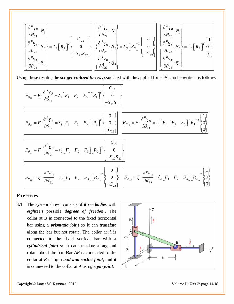
Exercises
3.1 The system shown consists of three bodies with
eighteen possible degrees of freedom. The
collar at B is connected to the fixed horizontal
bar using a prismatic joint so it can translate
along the bar but not rotate. The collar at A is
connected to the fixed vertical bar with a
cylindrical joint so it can translate along and
rotate about the bar. Bar AB is connected to the
collar at B using a ball and socket joint, and it
is connected to the collar at A using a pin joint.
Copyright © James W. Kamman, 2016 Volume II, Unit 3: page 15/18
Using the counting procedure discussed above, verify that the system has only one degree of freedom.
How many degrees of freedom does the system have if the joint at A is changed to a ball and socket
joint? How many degrees of freedom does the system have if the collar at B is connected to the fixed
horizontal bar with a cylindrical joint?
Answers: 1 DOF as is; 3 DOF if ball and socket joint at A; 2 DOF if collar at B can rotate
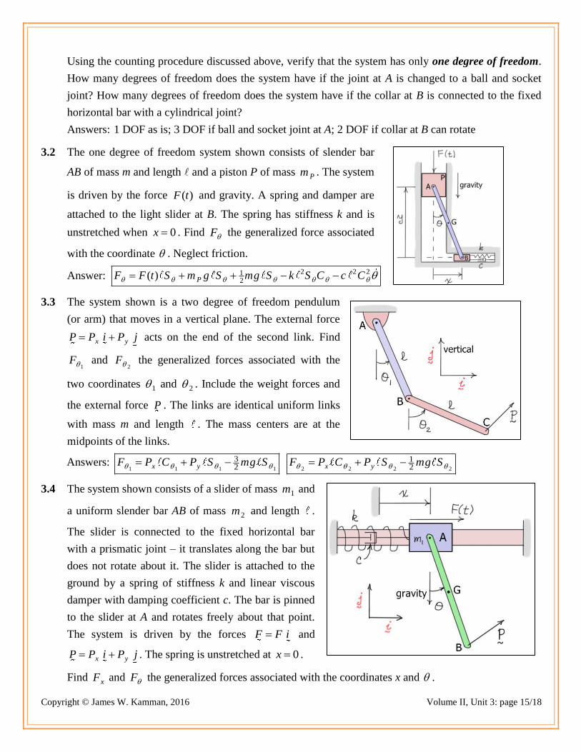
3.2 The one degree of freedom system shown consists of slender bar
AB of mass m and length and a piston P of mass Pm . The system
is driven by the force ( )F t and gravity. A spring and damper are
attached to the light slider at B. The spring has stiffness k and is
unstretched when 0x . Find F the generalized force associated
with the coordinate . Neglect friction.
Answer: 2 2 21
2( ) PF F t S m g S mg S k S C c C
3.3 The system shown is a two degree of freedom pendulum
(or arm) that moves in a vertical plane. The external force
x yP P i P j acts on the end of the second link. Find
1F and
2F the generalized forces associated with the
two coordinates 1 and 2 . Include the weight forces and
the external force P . The links are identical uniform links
with mass m and length . The mass centers are at the
midpoints of the links.
Answers: 1 1 1 1
32x yF P C P S mg S
2 2 2 2
12x yF P C P S mg S
3.4 The system shown consists of a slider of mass 1m and
a uniform slender bar AB of mass 2m and length .
The slider is connected to the fixed horizontal bar
with a prismatic joint – it translates along the bar but
does not rotate about it. The slider is attached to the
ground by a spring of stiffness k and linear viscous
damper with damping coefficient c. The bar is pinned
to the slider at A and rotates freely about that point.
The system is driven by the forces F F i and
x yP P i P j . The spring is unstretched at 0x .
Find xF and F the generalized forces associated with the coordinates x and .

Copyright © James W. Kamman, 2016 Volume II, Unit 3: page 16/18
Answers: x xF F P k x cx 212x yF P C P S m g S
3.5 The two degree of freedom system shown consists of two
bodies – disk D and slender bar B. The disk has radius R and
mass Dm . The slender bar has length and mass m. The unit
vector set ( , , )D i j k are fixed in the disk along the X , Y
and Z axes. The rotation of the disk about the Z axis is given by
the angle ( ) , and the rotation of the bar relative to the
disk about the X axis is given by the angle . A rotational
spring-damper located at pin P restricts the motion between the
bar and the disk. The spring has stiffness k and the linear,
viscous damper has damping coefficient c. An external force
X Y ZF F i F j F k is applied to the end of the bar.
A motor torque M is applied by the ground to the disk about the Z axis, and a motor torque M is
applied by the disk to the bar at P. Find F and F the generalized forces associated with the
coordinates and .
Answers: XF M F b S 12 Y ZF M mg S k c F C F S
3.6 The system shown is a three-dimensional double
pendulum or arm. The first link is connected to
ground and the second link is connected to the first
with universal joints at O and A, respectively. The
ground frame is 1 2 3: , ,R N N N and the link frames
are 1 2 3: , , ( 1, 2)ii i iL n n n i . The orientation of 1L
is defined relative to R and the orientation of 2L is
defined relative to 1L each with a 1-3 body-fixed
rotation sequence.
Link OA is oriented relative to the ground frame by first rotating through an angle 11 about the 1N
direction, and then rotating about an angle 12 about the 13n direction. Link AB is oriented relative to
link OA by rotating first through an angle 21 about the 11n direction, and then through an angle 22
about the 23n direction. The lengths of the links are 1 and 2 with mass centers are at their midpoints.
The system is driven by gravity and by four motor torques, one on each axis of the universal joints. The
four motor torques can be written as follows

Copyright © James W. Kamman, 2016 Volume II, Unit 3: page 17/18
11 11 1M M N 1
12 12 3M M n 1
21 21 1M M n 2
22 22 3M M n
The two constraint torques transmitted through the joints can be written as
11 3O OT T N n 1 2
1 3A AT T n n .
Find 11
F , 12
F , 21
F and 22
F the generalized forces associated with the four orientation angles. In the
process, show that the contribution of the constraint torques OT and AT are zero. Assume the 2N
direction is vertical.
Answers:
Recall that matrix 1R transforms components from the base frame (R) to 1L , and the matrix 2R
transforms components from 1L to 2L .
11 11 1 1 1
12
12 21
1 2 1 2 2 1 2
12 12 21 22 12 22
1 111 1 1 11 12 1 2 11 12 2 2 22 11 12 21 22 11 122 2
12
12
0
0 0 0
0
0 0 0 0 0 0
T
T T T
F M W R
C
S S
W R W R R
C S C S C C
M W S C W S C W S S S C C S C S
21 22 11C C
12 12 1 1 1
21
1 2 1 2 2 1 2
21 22
1 112 1 1 11 12 1 2 11 12 2 2 22 11 12 21 22 11 122 2
12
12
1
0 0 0
0
1
0 0 0 0 0 0
0
T
T T T
F M W R
C
W R W R R
S S
M W C S W C S W S C C C C C S
21
121 2 2 1 2 21 2 2 21 22 11 12 21 22 112
22
12
0
0 0 0T T
F M W R R M W S C C C C C S
C
22 22 2 2 1 2
122 2 2 22 11 12 21 22 11 12 21 22 112
12
1
0 0 0
0
T TF M W R R
M W C C S C S C C S S S

Copyright © James W. Kamman, 2016 Volume II, Unit 3: page 18/18
References:
1. L. Meirovitch, Methods of Analytical Dynamics, McGraw-Hill, 1970.
2. T.R. Kane, P.W. Likins, and D.A. Levinson, Spacecraft Dynamics, McGraw-Hill, 1983
3. T.R. Kane and D.A. Levinson, Dynamics: Theory and Application, McGraw-Hill, 1985
4. R.L. Huston, Multibody Dynamics, Butterworth-Heinemann, 1990
5. H. Baruh, Analytical Dynamics, McGraw-Hill, 1999
6. H. Josephs and R.L. Huston, Dynamics of Mechanical Systems, CRC Press, 2002
7. R.C. Hibbeler, Engineering Mechanics: Dynamics, 13th Ed., Pearson Prentice Hall, 2013
8. J.L. Meriam and L.G. Craig, Engineering Mechanics: Dynamics, 3rd Ed, 1992
9. F.P. Beer and E.R. Johnston, Jr. Vector Mechanics for Engineers: Dynamics, 4th Ed, 1984
Top Related