![Ontology-based Personalised Course Recommendation Framework · 2019. 1. 8. · Ontology-based Personalised Course Recommendation Framework MOHAMMED E. IBRAHIM1,2(Member, ... [25]](https://static.fdocuments.us/doc/165x107/603c6d90a65f9240f444d993/ontology-based-personalised-course-recommendation-framework-2019-1-8-ontology-based.jpg)


Languages
Pages
Legal


An Intelligent Recommendation Framework
for Student Counselling Management
in Thai Private Universities
Kanokwan Kongsakun
B.B.A. (Business Computer) Prince of Songkla University, Thailand
M.S. Ind. Ed. (Computer and Information Technology),
King Mongkut’s University of Technology Thonburi, Thailand
This thesis is presented for the Degree of
Doctor of Information Technology of
Murdoch University
September 2013

ii
Declaration
I declare that this thesis is my own account of my research and contains as its main
content work which has not previously been submitted for a degree at any tertiary
education institution.
Kanokwan Kongsakun
September 27, 2013

iii
Acknowledgements
The doctoral thesis could have not been completed, if I have not received the support
from many important people and supportive organisations in my life. This is a good
opportunity to thank all of them.
In countless ways, I have received love and support from my wonderful family. I would
like to thank my parents for the endless love and caring, two older sisters for love and
assistance, and all my cousins for their encouragement to further my study in Australia.
I am grateful to the Scholarship Committee of Hatyai University, Thailand for the
provision of a Postgraduate Study Scholarship and supports for my doctoral degree at
Murdoch University, Western Australia. Especially, I am grateful to Ajarn Tharnpas
Sattayarak, Vice President for Administration, Hatyai University, who assists me with
many supports.
I would also like to express my utmost gratitude to my principal supervisor, Associate
Professor Dr. Lance Chun Che Fung who has worked very hard to guide, support,
encourage and critique my work throughout the period of my study. I am also deeply
grateful for his supervision and efforts for the invaluable insight and experiences in my
academic career. I would like to express my gratefulness to my co-supervisor, Associate
Professor Dr. Kevin Kok Wai Wong for his advice, helpful comments and excellent
guidance in my research.

iv
I would like to thank Associate Professor Dr. Tanya McGill for the advice and teaching
on the subject of research methodology. I appreciate my fellow student, Mr Jesada
Kajornrit and his wife, Usarom Pongsarak, for their help and advice. My thanks are due
to Mr John Covate who assisted me at the beginning of this study, to my colleagues in
Thailand, and thanks to all my housemates, office mates and friends for their friendship
during my time in Perth.
Finally, I am deeply grateful to my wonderful husband, Michael Steven Watkins, for
love, understanding, inspiration, encouragement and support to empower me to finish
my research for the doctoral study. Thank you very much for standing by my side
during the study.

v
Abstract
This study proposed a framework for an Intelligent Recommendation System for
private universities in Thailand. Choosing a program of study for students is
significant due to the commitment involved and the potential career opportunities.
However, many students have enrolled in course majors without receiving any
advice from appropriate authorities or university services. This could have
potential mismatch between a student’s background, personal interests and
capability, with the particular course being taken up. This may lead to low
retention and dropouts. In order to improve the academic management processes,
many universities are developing innovative information systems and services with
an aim to enhance efficiency and student relationship. One of the key initiatives is
the development of Student Relationship Management Systems (SRM) and among
their functions, is the provision of recommendation and advice for students. The
proposed system in this study examined the correlation between up to 11,000
student records and their academic performance. The system focuses on the
following outcomes: programme and activity recommendation, likely overall GPA
and results in each year, Identification of postgraduate students and potential
dropouts. Association Rules and K-Means Clustering have been used together with
three classification techniques: Artificial Neural Networks (ANN), Decision Tree
(DT) and Support Vector Machines (SVM). Ensemble and the Modular Artificial
Neural Networks based on Optimised Weight of Subspace Reconstruction
(MANN-OWSR) have also been used to combine the learning models for
improved performance. Results from the experiments will be useful for counsellors
and academic staff in suggesting appropriate recommendations for the students.

vi
List of publications related to this thesis
JOURNAL
[P1] K. Kongsakun and C. C. Fung, "Neural Network Modelling for an Intelligent Recommendation System Supporting SRM for Universities in Thailand” In WSEAS TRANSACTIONS on COMPUTERS. Issue 2, Vol. 11, February 2012, pp.34-44.
[P2] K. Kongsakun, J. Kajornrit and C. C. Fung, Neural Network Modelling for an Intelligent Recommendation System Supporting SRM for Universities in Thailand. In The Asian International Journal of Science and Technology in Production and Manufacturing Engineering (AIJSTPME), July – September, 2012, Vol. 5, No. 3
CONFERENCE PROCEEDINGS
[P3] K. Kongsakun, J. Kajornrit and C.C. Fung, Understanding Student Relationship Management and Its effects on University students. In the Postgraduate Electrical Engineering and Computing Symposium (PEECS 2009), WA, Australia. October 2009.
[P4] K. Kongsakun, and C.C. Fung, a Recommendation System for Student Relationship Management. In Proceeding of the 8th International Conference on E-Business (INCEB 2009), Bangkok, Thailand, 28th-29th October 2009.
[P5] K. Kongsakun, C. C. Fung, S. Borirug and W. Philuek, An Intelligent Recommendation System Framework for Student Relationship Management. In Proceedings of the “World Academy of Science, Engineering and Technology”, Penang, Malaysia, volume 62, February 2010.
[P6] K. Kongsakun and C. C. Fung, Developing an Intelligent Recommendation System for a Private University in Thailand. In Proceedings of the International Association for Computer Information Systems (IACIS), Las Vegas, USA, 6-9 October, 2010.
[P7] K. Kongsakun, J. Kajornrit and C. C. Fung, Neural Network Modelling for an Intelligent Recommendation System Supporting SRM for Universities in Thailand. In Proceedings of the 8th International Conference on Computing and Information Technology (IC2IT), Pattaya city, Thailand, 9-10 May, 2012.
[P8] K. Kongsakun, Tuchtawan Chanakul and C. C. Fung, Decision Tree Modelling for an Intelligent Recommendation System Supporting SRM for Universities in Thailand. In Proceeding of the International Conference on Computer and Information Technology (ICCIT’2012), Bangkok, Thailand, 16-17 June, 2012.
[P9] K. Kongsakun, Prediction of Likelihood of Overall Results from Freshmen Using a Combined Classifier in a Recommendation System. In Proceeding of the

vii
Postgraduate Electrical Engineering and Computing Symposium (PEECS 2012), Curtin University, WA, Australia, 9 November 2012.
[P10] K. Kongsakun, C.C. Fung and K.W. Wong, Drop-out Identification model using Data Mining for an Intelligent Recommendation System for Universities in Thailand. In Proceeding of the Hatyai Symposium 2013, Songkla, Thailand, 10 May 2013.
[P11] K. Kongsakun, An improved recommendation model using linear regression and clustering for a private university in Thailand. In Proceeding of the International Conference on Machine Learning and Cybernetics (ICMLC 2013),Tianjin, China, 14-17 July 2013.

viii
Contributions of this thesis
In general, recommendations in university are provided by counsellors or advisers
without any analysis of the information from past students. In this thesis, an intelligent
recommendation system for university students is proposed. The contributions in this
thesis which have been published previously in the list of publications related to this
thesis are summarised below.
Key Contributions Supportive papers
A review of various techniques in recommendation systems, data mining and intelligent techniques, and report on the proposed framework.
Conference Papers
[P3], [P4] and [P5]
Reported on the use of combined classifiers for GPA prediction in a recommendation system to improve the performance accuracy.
Conference Paper
[P9]
Reported on the use of K-Mean clustering and comparison of results obtained from other approaches. Also, reported on the proposed techniques and results based on artificial neural networks and decision tree used in this study together with comparison with other approaches.
Conference Papers
[P6], [P7], [P8]
Journal Papers
[P1] and [P2]
Reported on the proposed framework and results based on clustering, together with ANN, Decision Tree and SVM including Ensemble and MANN-OWSR for dropout identifications and comparison with other approaches.
Conference Paper
[P10] [P11]

ix
Contents
Acknowledgements ........................................................................................................ iii
Abstract ............................................................................................................................ v
List of publication related to this thesis ....................................................................... vi
Contributions of this thesis ......................................................................................... viii
List of Figures ................................................................................................................ xii
List of Tables ................................................................................................................ xiv
List of Abbreviations .................................................................................................... xvi
Chapter 1: Introduction ................................................................................................. 1
1.1 Background ............................................................................................................. 1 1.2 Objective ................................................................................................................. 4 1.3 Methodology ........................................................................................................... 4 1.4 Thesis Outline ......................................................................................................... 6
Chapter 2: Background .................................................................................................. 9
2.1 Introduction ............................................................................................................. 9 2.2 University System in Thailand ................................................................................ 9
2.2.1 University types ............................................................................................... 9 2.2.2 University admission process ......................................................................... 11 2.2.3 Student relationship management in Thai universities .................................. 13 2.2.4 Student counselling in universities ................................................................. 15 2.2.5 Background information on students ............................................................. 16 2.2.6 Justification for the proposed recommendation system ................................. 17
2.3 Intelligent Techniques for the Proposed Recommendation System ...................... 18 2.3.1 Artificial Neural Networks ............................................................................. 19 2.3.2 Decision tree ................................................................................................... 20 2.3.3 Support vector machine .................................................................................. 21 2.3.4 Association rules ............................................................................................ 22 2.3.5 K-means clustering ......................................................................................... 23 2.3.6 Confidence-weighted voting ensemble .......................................................... 23 2.3.7 Modular Artificial Neural Networks-Optimised Weight of Subspace
Reconstruction ............................................................................................... 24 2.3.8 Evaluation metrics of the intelligent recommendation system ...................... 26
2.4 Summary ............................................................................................................... 27
Chapter 3: Framework of the Proposed Recommendation System ......................... 28
3.1 Introduction ........................................................................................................... 28

x
3.2 An Overview of the Proposed Recommendation System ..................................... 28 3.3 Description of the Modules and Their Purposes ................................................... 29
3.3.1 Module 1: likely overall GPA ........................................................................ 29 3.3.2 Module 2: ranked programme recommendation ............................................ 29 3.3.3 Module 3: likely GPA for each semester ....................................................... 30 3.3.4 Module 4: ranked activities recommendation ................................................ 31 3.3.5 Module 5: programme completion identification .......................................... 31 3.3.6 Module 6: postgraduate study identification .................................................. 31
3.4 Description of Parameters Used in this Study ....................................................... 32 3.4.1 UniID .............................................................................................................. 34 3.4.2 GPAs .............................................................................................................. 34
3.4.2.1 Overall GPA ............................................................................................ 35 3.4.2.2 GPA each semester ................................................................................. 35 3.4.2.3 Previous school GPA .............................................................................. 36 3.4.2.4 Postgraduate GPA ................................................................................... 36
3.4.3 Previous major ............................................................................................... 37 3.4.4 Type of school ................................................................................................ 37 3.4.5 Number of awards .......................................................................................... 38 3.4.6 Talents and interests ....................................................................................... 39 3.4.7 Motivation channels ....................................................................................... 39 3.4.8 Admission round ............................................................................................ 40 3.4.9 Guardian occupation ...................................................................................... 41 3.4.10 Gender .......................................................................................................... 41 3.4.11 Activity type ................................................................................................. 41 3.4.12 University major ........................................................................................... 42
3.5 Methodology ......................................................................................................... 44 3.5.1 Data pre-processing ........................................................................................ 44 3.5.2 Data analysis (hybrid classification association recommendation models) ... 45 3.5.3 Validation of model based on intelligent recommendation system ............... 47
Chapter 4: Programme and Activity Recommendation ............................................ 48
4.1 Introduction ........................................................................................................... 48 4.2 Objectives .............................................................................................................. 49 4.3 Input and Output Variables Selection ................................................................... 49 4.4 Experiment Methodology and Design .................................................................. 52 4.5 Intelligent Technique Used ................................................................................... 54 4.6 Experiment Results ............................................................................................... 55
4.6.1 Example results of ranked programme and activity recommendations based on GRI algorithm ................................................................................. 56
4.6.2 Example results of ranked programme and activity recommendations based on GRI and K-means clustering .......................................................... 61
4.7 Conclusion and Discussion ................................................................................... 63 Chapter 5: Grade Point Average Prediction and Postgraduate Identification ....... 65
5.1 Introduction ........................................................................................................... 65 5.2 Objectives .............................................................................................................. 65 5.3 Input and Output Variables Selection ................................................................... 66 5.4 Intelligent Techniques ........................................................................................... 68 5.5 Experimental Methodology and Design ................................................................ 70

xi
5.6 Experiment Results ............................................................................................... 72 5.6.1 First comparison between SVM, ANN and CHAID ...................................... 72 5.6.2 Second comparison of the ANN, CHAID and ensemble models .................. 74 5.6.3 Third comparison using MANN-OWSR, SVM and ensemble in overall
GPA and GPA of each semester .................................................................... 76 5.6.4 Third comparison of MANN-OWSR, SVM and CHAID in the
postgraduate identification module ................................................................ 78 5.7 Conclusion and Discussion ................................................................................... 79
Chapter 6: Dropout Identification ............................................................................... 81
6.1 Introduction ........................................................................................................... 81 6.2 Objectives .............................................................................................................. 81 6.3 Input and Output Variables Selection ................................................................... 82 6.4 Experimental Methodology and Design ................................................................ 83 6.5 Experimental Results ............................................................................................ 85
6.5.1 First comparison of classification techniques ANN, CHAID and SVM ....... 85 6.5.2 Results from K-means clustering ................................................................... 86 6.5.3 Comparing results from three models using data from Cluster 1: second
comparison ..................................................................................................... 87 6.5.4 Comparison of results based on data from Cluster 2 ..................................... 88 6.5.5 Fourth comparison between Ensemble 1 and Ensemble 2 ............................. 90 6.5.6 Fifth comparison between MANN-OWSR and the best ensemble ................ 91
6.6 Conclusion and Discussion ................................................................................... 92
Chapter 7: Conclusion and Future Work ................................................................... 94
7.1 Introduction ........................................................................................................... 94 7.2 Summary of Findings ............................................................................................ 94
7.2.1 Programme and activity recommendations .................................................... 94 7.2.2 Grade point average prediction and postgraduate identification .................... 95 7.2.3 Dropout identification: programme completion identification and dropout
identification modules ................................................................................... 96 7.3 Discussion on Future Work ................................................................................... 97 7.4 Conclusion ............................................................................................................. 98
References ...................................................................................................................... 99
Appendix ...................................................................................................................... 111

xii
List of Figures
Figure 1.1: Process of developing the proposed recommendation system ....................... 5
Figure 1.2: Thesis outline .................................................................................................. 8
Figure 2.1: Relationship marketing model for student retention [31] ............................. 14
Figure 2.2: A multilayer feed-forwards network ............................................................ 19
Figure 2.3: Development of the MANN-OWSR model [2] ............................................ 24
Figure 2.4: The vector of a new student as X1Y1 within a boundary of β. Only the
training data within β are used for the MANN-OWSR model [2] ................. 25
Figure 2.5: Training data used in the MANN-OWSR model [2] .................................... 25
Figure 3.1: Percentage of participants’ opinion in relation to independent variables,
the likely study level and programme of study .............................................. 33
Figure 3.2: Proposed intelligent recommendation system based on the Hybrid
Classification Association framework ........................................................... 44
Figure 4.1: Number of undergraduate students by programme of study (2001–2007) ... 50
Figure 4.2: Process to compare performance of GRI for ranked programme and
activity recommendations .............................................................................. 52
Figure 4.3: Flowchart to derive recommendation for three ranked programme
majors and activities ....................................................................................... 53
Figure 4.4: Distribution of the rules in each ranking ...................................................... 59
Figure 4.5: Comparison of the accuracy between ranked programme and activity
recommendations ........................................................................................... 60
Figure 4.6: Comparison of mean absolute error between ranked programme and
activity recommendations .............................................................................. 60
Figure 4.7: Comparison of accuracies between ranked programme and activity
recommendations ........................................................................................... 62
Figure 4.8: Comparison of mean absolute errors between ranked programme and
activity recommendations .............................................................................. 63
Figure 5.1: Number of postgraduate students in each postgraduate programme
(2001–2009) ................................................................................................... 66
Figure 5.2: Process for determining the best GPA recommendation model ................... 70
Figure 5.3: Accuracy rate of the classification techniques ............................................. 73

xiii
Figure 5.4: Comparison of MAE from the first process ................................................. 73
Figure 5.5: Comparison of the accuracy rate between ANN, CHAID and ensemble ..... 75
Figure 5.6: Comparison of MAE between ANN, CHAID and ensemble ....................... 75
Figure 5.7: Comparison of the accuracy between MANN-OWSR, SVM and
ensemble ......................................................................................................... 77
Figure 5.8: Comparison of MAE between MANN-OWSR, SVM and ensemble .......... 77
Figure 5.9: Comparison of the accuracy between MANN-OWSR, SVM and CHAID .. 78
Figure 5.10: Comparison of MAE between MANN-OWSR, SVM and CHAID ........... 79
Figure 6.1: Number of undergraduate students, including dropouts, by programme
of study (2001–2007) ..................................................................................... 82
Figure 6.2: Process for determining the student dropout identification model ............... 84
Figure 6.3: Comparison of the accuracy between classification techniques ................... 86
Figure 6.4: Number of data in each cluster from K-means clustering ............................ 87
Figure 6.5: Comparison of accuracy based on dataset from Cluster 1 ............................ 88
Figure 6.6: Comparison of accuracy based on data from the second cluster .................. 89
Figure 6.7: Comparison of accuracy of SVM and ANN ensembles ............................... 90
Figure 6.8: Comparison of accuracy of ensemble and MANN-OWSR .......................... 91
Figure 6.9: Accuracy of ensemble in comparison to the single SVM model ................. 92

xiv
List of Tables
Table 2.1: Enrolment numbers in higher education institutions in Thailand [26] .......... 11
Table 3.1: Statistical parameters for the categorised GPAs ............................................ 34
Table 3.2: Six classes of overall GPA based on statistics ............................................... 35
Table 3.3: Five classes of previous school GPA ............................................................. 36
Table 3.4: Five classes of postgraduate GPA results ...................................................... 37
Table 3.5: Classes of previous major .............................................................................. 37
Table 3.6: Classes of type of school ................................................................................ 38
Table 3.7: Class of number of awards ............................................................................. 38
Table 3.8: Class of talents and interests .......................................................................... 39
Table 3.9: Class of motivation channels ......................................................................... 40
Table 3.10: Classes of admission round .......................................................................... 40
Table 3.11: Classes of guardian occupation .................................................................... 41
Table 3.12: Classes of gender ......................................................................................... 41
Table 3.13: Classes of activity type ................................................................................ 42
Table 3.14: Classes of university major .......................................................................... 42
Table 3.15: Samples of variables in the training sample dataset for likely overall
GPA ................................................................................................................ 43
Table 4.1: Variables used in the ranked programme and activity modules .................... 51
Table 4.2: Example results of ranked programme recommendation .............................. 54
Table 4.3: Example results of ranked activity recommendation ..................................... 54
Table 4.4: Example results of rules extraction by GRI for ranked programme
recommendations ........................................................................................... 56
Table 4.5: Example results of rules extraction by GRI for ranked activity
recommendation ............................................................................................. 57
Table 4.6: A comparison of the accuracy between the ranked programme and
activity recommendations .............................................................................. 59
Table 4.7: Comparison of mean absolute error between ranked programme and
activity recommendations .............................................................................. 60
Table 4.8: Comparison of accuracies between ranked programme and activity
recommendations ........................................................................................... 61

xv
Table 4.9: Comparison of mean absolute errors between ranked programme and
activity recommendations .............................................................................. 62
Table 5.1: Variable names and data types in each module ............................................. 67
Table 5.2: Example results for likely overall GPA and likely GPA in each semester .... 72
Table 5.3: Example results for postgraduate identification ............................................ 72
Table 5.4: Accuracy rate from the first process .............................................................. 72
Table 5.5: Comparison of MAE from the first process ................................................... 73
Table 5.6: Comparison of the accuracy rate between ANN, CHAID and ensemble ...... 74
Table 5.7: Comparison of MAE between ANN, CHAID and ensemble ........................ 75
Table 5.8: Comparison of the accuracy between MANN-OWSR, SVM and
ensemble ......................................................................................................... 76
Table 5.9: Comparison of MAE between MANN-OWSR, SVM and ensemble ............ 77
Table 5.10: Comparison of the accuracy between MANN-OWSR, SVM and
CHAID in the postgraduate identification module ........................................ 78
Table 5.11: Comparison of MAE between MANN-OWSR, SVM and CHAID ............ 79
Table 6.1: Name and type of input and output data ........................................................ 83
Table 6.2: First comparison of classification technique accuracy .................................. 86
Table 6.3: Number of clusters and iterations by K-means clustering ............................. 86
Table 6.4: Comparison of results based on data from Cluster 1 ..................................... 87
Table 6.5: Comparison of results from the second cluster .............................................. 88
Table 6.6: Results of comparison between Ensemble 1 and 2 ........................................ 90
Table 6.7: Accuracies from the best ensemble and MANN-OWSR ............................... 91
Table 6.8: Comparison of SVM cluster ensemble and single SVM model .................... 92

xvi
List of Abbreviations
Abbreviation Definition
ANN Artificial Neural Network
AR Association Rules
BP Back Propagation
CAAR Classification based on Atomic AR
CHAID Chi-squared Automatic Interaction Detector
CRM Customer Relationship Management
CUAS Central University Admissions System
DT Decision Tree
GPA Grade Point Average
GRI Generalised Rule Induction
HCAF Hybrid Classification Association Framework
HE Higher Education
HEI Higher Education Institutes
MAE Mean Absolute Error
MANN-OWSR Modular ANNs based on Optimised Weight of Subspace
Reconstruction
MLP Multilayer Perceptron
RMSE Root of the Mean Square Error
SD Standard Deviation
SRM Student Relationship Management
SVM Support Vector Machine

1
Chapter 1: Introduction
1.1 Background
Higher education (HE) is essential to the development of a country’s long-term
economic performance and productivity [1]. As it requires substantial investments and
resources, one of the key objectives of higher education institutes (HEIs) is to focus on
improving student completion rates in respective programmes. In Thailand, records
reveal that there is room for improvement in this area. Novoa, Curado and Machado [3]
found that one cause can be attributed to the high number of student dropouts. This has
led to wasted resources and a reduced number of graduates to meet the demands of
industry and the community. There are many reasons why a student may choose to drop
out, such as finding that the programme is unsuitable. This problem usually originates at
enrolment when the student selects or is recommended an unsuitable programme of
study.
Previous studies have investigated the issues that can lead to student dropouts at
university. One of these issues is depression. This can occur when the student is unable
to cope with study, which is a common problem among tertiary students. This affects
the student’s behaviour, motivation level, concentration, feeling of self-worth and mood
and can eventually lead to the student electing to drop out [4]. From a university
perspective, causes for dropouts are related to the allocation of resources and inability to
recruit students of appropriate calibre with a high probability of completion.
Inappropriate management decisions can lead to unoccupied student placements and
loss of potential tuition fees when students dropout. The problem of student retention in
HE can also be attributed to low student satisfaction and student transfer [5]. In addition
to these causes, previous studies have found that the quality and convenience of support
services influence Thai students to change educational institutes in HE [6]. Therefore, it
is necessary to meet student needs and to match their capabilities with suitable
programmes of study in HE recruitment and enrolment processes. Understanding
student needs will enhance their learning experience, increase their chances of success
and reduce resource wastage that is due to dropouts and change of programs.

2
With a limited supply of resources and increasing competition for students in Thailand’s
HE sector, universities and institutes are focusing their efforts on increasing the rate of
student retention and completion. In addition, reputation is being used increasingly to
measure the university’s quality and performance [7]. One aspect of such measurement
is based on factors that affect student satisfaction. Gatfield [8] stated that it is vital that
HEIs concentrate on quality through accreditation processes and various aspects of
quality services from a student perspective.
Archer and Cooper [9] confirmed that the provision of counselling services is an
important factor contributing to students’ academic success. Urata and Takano [10]
stated that the essence of student counselling should include advice on career guidance,
identification of learning strategies, handling of interpersonal relationships, along with
self-understanding of the mind and body. A key aspect of student services is to provide
counselling on programme guidance because this will assist the students in their
enrolment decisions and future university experience. Although many students choose
particular programmes of study because of job opportunities, issues may arise if a
student is not interested in the career or if the programme is not suitably matched with
the student’s capabilities [11]. Therefore, to assist with student retention, HEIs need to
determine how they can attract or recruit students and how they can match students to
appropriate programmes of study to achieve a high completion rate.
In the business world, organisations and corporations rely on successful relationships
with customers and they dedicate a large amount of effort to gaining and maintaining
customers and establishing successful relationships with those customers [12].
Customer Relationship Management (CRM) is a management concept aimed at
enhancing customer satisfaction and improving the relationship between the
organisation and its customers [13]. Student Relationship Management (SRM) is a
similar concept applied in the academic world. CRM has been defined as:
a fundamental strategic orientation which is pursued by all members of a
company in order to increase customer satisfaction, customer loyalty and the
benefit for the consumer as well as for the company during the entire supplier-
customer-relationship [14].

3
In educational institutes, students could be considered a form of customer and, as such,
the objective of SRM is to increase student satisfaction and loyalty for the benefit of the
institute. SRM can be considered similar to CRM because it aims to develop and
maintain a close relationship between the institute and the students by supporting the
administrative process and monitoring the students’ academic activities and
performance. Piedade and Santos [15] explained that SRM involves the identification of
performance indicators and behavioural patterns that characterise the students and the
situations under which they are supervised. In addition, SRM is:
understood as a process based on the student acquired knowledge, whose main
purpose is to keep a close and effective students institution relationship
through the closely monitoring of their academic activities along their
academic path.
Therefore, similarly to CRM, SRM is considered an important means of enhancing
student satisfaction [12].
The HE sector in Thailand consists of 79 public and 71 private HEIs and 19 community
colleges [16]. The Thai education system is based on government policies. Gamage [11]
found that:
another challenge faced by the higher education in Thailand that is pushing the
public universities to become ‘autonomous universities’, or public
corporations with more administrative and financial autonomy.
This causes intense competition between private and government universities in
Thailand. Both sectors are competing fiercely to attract students that may eventually
affect the university’s sustainability [17]. Therefore, HEIs in Thailand need to maintain
or obtain sufficient student numbers. This means that private universities need to
compete with other universities and enhance their reputation to gain student attention.
For example, Hatyai University, a private university in the south of Thailand, faces
various challenges, including competition with other universities, change of government
policies and political unrest in the southern part of Thailand. However, some factors are
within the control or influence of the university, such as student recruitment, student
enrolment and student retention. For example, as a typical private university, Hatyai
University has strategies that aim to increase student retention and completion rates,

4
improve the university’s reputation and enhance student satisfaction through the
provision of student services, such as programme advice and career guidance. To
achieve these aims, the university needs to establish some form of SRM approach to
ensure successful relationships with its students.
Within this context, this research study aimed to investigate and develop an intelligent
system to provide academic recommendations for new students based on historical
records of students who have successfully completed their programmes. Moreover, this
project focused on techniques that enabled the recommendation system to improve
student services, which, in turn, supported SRM by assisting students to choose the
most appropriate programme for their study at university. This focus ensured that the
objective was met, which was to improve completion rates in HEIs.
1.2 Objective
The objective of this research was to develop and apply intelligent techniques and
methodologies to a recommendation system for recommending appropriate programmes
and activities to students. It also aimed to assess the likely overall grade point average
(GPA), as well as the GPA for each semester, for prospective students, new students
and current students. Other objectives including identifying students who were likely to
succeed in postgraduate study and identifying students who were likely to drop out
before graduation. The proposed techniques were implemented and evaluated based on
classification models in each of the techniques. Finally, the proposed techniques were
applied to determine the best model for achieving good results from the intelligent
recommendation system.
1.3 Methodology
The literature review found that few Thai universities used recommendation systems to
support SRM. The workflow of the development of the proposed system is illustrated in
Figure 1.1.

5
Figure 1.1: Process of developing the proposed recommendation system
This study used several processes to achieve its objectives. The first process involved
defining the research problems. This was followed by the data selection and pre-
processing data processes. The data analysis process was performed next and was
followed by the proposal of an intelligent recommendation system that makes
appropriate recommendations for students based on artificial intelligence and data-
mining techniques.
Figure 1.1 demonstrates that the data selection process was carried out after the research
problems were defined. This involved choosing the appropriate variables for the
training data and, as such, was an important step. The variables were based on survey
results provided by the university, which were based on the opinion and experience of
supervisors and counsellors who had been involved with the process. During the data
preparation process, pre-processing was used to organise the student records from the
university’s enterprise database. The data were then re-formatted in preparation for
processing by subsequent algorithms. Next, the data cleaning process was executed to
identify the parameters from the dataset, and missing data were either deleted or
completed with null values [18]. Preparation of the analytical variables was done in the

6
data transformation step or in a separate process. Validity of the data was then checked
against the legitimate range of values and data types.
The next step was data analysis, which included five techniques: Decision Tree (DT),
Artificial Neural Network (ANN), Support Vector Machine (SVM), Association Rules
(AR) and Clustering. The development process also involved a process for training,
validating and testing the model. The prediction models comprised of six modules
within the intelligent recommendation framework. The details of each module are
explained in the subsequent chapters. As there were multiple outputs from the various
modules, two aggregation models (ensemble and modular ANNs [MANNs] based on
Optimised Weight of Subspace Reconstruction [OWSR]) were employed to improve the
accuracy of the final results. In the final process, the results were compared and the
models that returned the best accuracy were chosen to determine the recommendations.
The proposed intelligent recommendation system was designed in such a way that it
forms an integral part of an online system for one or multiple private universities in
Thailand. The proposed system will be available for use by new students who may
access the online application during the enrolment process. Counsellors, staff and
university management will use the function for predicting subsequent years’ results to
provide support for students who are likely to be in need of help during their studies.
This information will enable the university to improve its resource management
processes. In particular, it could be used to improve the retention rate by providing
additional support to at risk students.
1.4 Thesis Outline
Chapter 1 provided an introduction to the research study. Chapter 2 will provide the
background of Thai university systems and will discuss the techniques to be used in the
recommendation system.
Chapter 3 will provide the framework of the proposed recommendation system, along
with the main idea and research methodology. It will also provide an overview of the
system, modules and purposes, including the parameters to be used in the system.

7
Chapter 4 will provide the module and process for the programme and activity
recommendations. This is a multiclass classification problem that aims to recommend
an appropriate programme and activities to the students; choice will be provided. The
objective of this module is to determine the most appropriate recommendation based on
past successful cases. The chapter will also describe the selection of input and output
variables and illustrate the proposed model with the experimental methodology and
design of the model. The subsequent section will discuss the intelligent technique
justification, which will be followed by the experimental results, discussion and
contributions.
Chapter 5 describes three modules: the likely overall GPA for prospective students or
new students, the likely GPA for students in each year and postgraduate identification,
which are forecasting problems. The model is trained with past GPA results from
student records for both GPA predictions and with past postgraduate student records for
the postgraduate identification. This chapter will discuss objectives, input and output
variable selection, experimental methodology and design and the justification of the
intelligent technique used. The experimental results are compared between different
techniques and variables to obtain the best result. Finally, the chapter will provide a
discussion and contributions.
Chapter 6 will describe the module for dropout identification. This is used not only for
new students but also for existing students in each year. The objective of this chapter is
to identify a possible dropout during a student’s programme of study. This will be
followed by input and output variable selection to support the model, experimental
methodology and design for the dropout identification model, intelligent technique
justification, experimental results, discussion and contributions.
The final chapter will conclude with a summary of the findings, contributions and
suggestions for future development. The thesis outline is illustrated in Figure 1.2.

8
Figure 1.2: Thesis outline

9
Chapter 2: Background
2.1 Introduction
In Thailand, one of the performance assessments for an educational institute is the
number and percentage of successful graduates. Educational institutes establish and
implement strategies to improve student satisfaction and academic development to
enhance the number of completions,, while upholding the quality and capabilities of the
graduates. Further, institutes use technology to assist students to succeed in their study.
In this thesis, an intelligent recommendation system based on artificial intelligence and
data-mining techniques is proposed to assist university students in choosing the
appropriate programme of study and the relevant subjects. The proposed system uses a
Hybrid Classification Association framework (HCAF) to aggregate results from
different techniques to enhance the performance of the system and confidence in the
outcomes. Recommendations on the programmes in which students should enrol are
important because they have implications on student commitment and the students’
families. This chapter provides the background of the university system in Thailand and
the justification for this study. This is followed by an explanation of the techniques and
methodology adopted in the proposed recommendation system.
2.2 University System in Thailand 2.2.1 University types
Thailand is a developing country with a population approaching 69 million of which 20
per cent are below the age of 14 and 9.2 per cent are above the age of 65 [19, 20].
Education is a significant factor in enhancing the capabilities and opportunities for the
people and improving the quality and standard of living. Sangnapaboworn, Director of
the International Education Development Center at the Office of the Education Council,
stated that HE in Thailand should be the highest level in the education system and
should focus on various fields of knowledge and research. It is expected that HEIs will
develop community leaders who will lead and establish sustainable solutions to address
the nation’s issues and to expand the areas of research and technology development.

10
Therefore, educating students at the university level will have a positive effect on the
nation’s economic growth, art, culture and social welfare through the development of
appropriate programmes and projects [21].
Thailand’s oldest HEI, Chulalongkorn University, was named after King
Chulalongkorn, Rama V, the Fifth King of the Chakri Dynasty and was established in
1916 [22]. Since then, HE in Thailand has grown considerably. For example, the 1933
Thammasat University Act was passed after the 1932 revolution, which laid the
foundation for commitment to HE with the establishment of the Thammasat University
in 1934 as an open university. The aim of this was to propagate the knowledge of law
and politics to the Thai people. In 1960, Thammasat University changed the open
admission to a restrictive selection process [22]. Details of the history of HE in Thailand
have been reported in [23].
Prior to 1969, HE in Thailand was a state monopoly. Towards the end of the 1960s, the
demand for tertiary study grew steadily [24] and, in 1969, the Thai government
established two open universities to meet the increasing demand. Private colleges and
universities have also been established since the passing of the Private College Act in
1969 [24, 25], and they have played an important role in their contribution to HE in
Thailand. In a survey conducted in July 2008, the number of HEIs in Thailand was 164
and comprised of 78 public universities, 67 private universities and 19 community
colleges, which provided educational opportunities for Thai communities [25, 26].
Along with the rise in HEIs came an increase in student numbers. The 1999 National
Education Act extended free basic education from 9 to 12 years and increased the
number of students further. A report by World Bank stated that the HEI gross enrolment
rates in Thailand have risen from seven per cent in 1987 to 56 per cent in 2005 [25]. A
survey conducted by the Bureau of International Cooperation in November 2008
showed that the number of university students in Thailand was 2,032,638 with 64,115
faculty members working in 145 institutes. The total number of students in the HE
sector was estimated to be 2.2 million with 91 per cent enrolled in undergraduate
programmes [27]. The student to faculty member ratio was estimated at 31:1. Table 2.1
provides information on enrolment numbers in Thai HEIs from 1998 to 2006 and
demonstrates that student numbers have increased substantially from year to year.

11
Table 2.1: Enrolment numbers in higher education institutions in Thailand [26]
Year Total PhD Master Graduate
diploma Bachelor
Lower
than
bachelor
1998 1,033,325 1,725 73,364 1,332 947,907 8,997
1999 1,012,285 2,362 78,131 1,914 918,421 11,457
2000 1,103,888 3,190 89,563 2,456 994,240 14,493
2001 1,179,569 5,080 107,825 2,015 1,046,501 18,148
2002 1,273,096 6,213 126,123 4,087 1,122,812 13,861
2003 1,850,864 7,711 126,863 4,958 1,631,693 79,639
2004 1,804,573 7,949 136,552 9,881 1,579,508 70,683
2005 1,900,203 11,623 154,338 6,401 1,656,427 71,414
2006 2,123,024 14,765 181,292 8,191 1,850,846 67,930
Table 2.1 shows that the number of enrolments has increased by almost double from
1998 (1,033,325) to 2006 (2,123,024). In particular, the number of PhD enrolments has
grown dramatically from 1,725 in 1998 to 14,765 in 2006. These statistics indicate a
significant increase in the number of enrolments at Thai universities.
2.2.2 University admission process
The academic year in Thai HEIs is divided into two semesters. The first semester
normally runs from June to September and the second semester runs from November to
March. School breaks (2–4 weeks) occur between these two semesters in October.
During the long summer break from April to May, many universities provide an
optional short semester, which is known as the summer semester.
Currently, there are approximately 9,300 study programmes, ranging from lower
undergraduate to PhD degree programmes, in both public and private universities [28].
As in other countries, the degree system in Thailand provides bachelor, master and PhD

12
degrees and a bachelor degree is normally a four-year programme. The exceptions are
the pharmacy and architecture programmes, which are five-year programmes, and the
dental surgery, medicine and veterinary medicine PhD programmes, which are all six-
year programmes. A master’s degree requires two years of full time study, which can
incorporate two forms of study: course work and research. Similarly, PhD degrees
include both course work and research study, and the programmes typically take three to
five years to complete [26]. During the study period, students spend most of their time
at the university and many have to live away from home. This can lead to social
challenges for some students, which can often affect their studies. If a student has
chosen a programme that is not suitable for him or her, this will put additional pressure
on the student and may lead to drop out or failure.
To gain admission to university, students have to fulfil certain entrance requirements.
Specifically, they need to participate in the assessment organised by the Central
University Admissions System (CUAS), which commenced in 2006. The CUAS
replaced the national entrance examination, which had been used for over four decades.
The CUAS aims to enable each individual student to study in one of the programmes
offered by the public universities. However, students who do not receive an offer from a
public university or who do not take the CUAS assessment have to consider alternate
options, such as private universities, open universities or Rajaphat universities.
There are other reasons why students may choose to enrol in private universities. For
example, they may select programmes based on reasons such as a particular programme
is not offered at the public universities, the proximity of the private university to their
home, examples or advice received from friends and parents, preferred learning modes
are offered or a better resourced environment. These students need to meet the financial
requirements, such as higher tuition and related fees, to study at the private universities.
However, some students may obtain education loans from the government. In 2006,
there were 1,846,301 students enrolled in public universities, including open
universities, and 276,723 students enrolled in private universities, making up
approximately 15 per cent of the overall student population in the HE sector [29].

13
2.2.3 Student relationship management in Thai universities
With a focus on private universities providing better services to students, one issue that
requires attention is the problem of low student retention. This problem can be
attributed to low student satisfaction, student transfers and dropouts [5] and leads to a
reduction in enrolment numbers and revenue and an increase in the cost of replacement.
Conversely, it was found that the quality and convenience of support services are
factors that may influence students to stay or change education institutes [6, 16]. An
understanding of the available information can assist student management, student
services and market operation. In addition, it is important to develop strategies to
maintain and enhance student satisfaction to achieve the above objectives. One
approach involves the establishment of an SRM system. A definition of SRM can be
adopted from the established practices of CRM in businesses, which focuses on
customers and aims to establish effective competition and new strategies to improve an
organisation’s performance [30]. SRM is used within the education sector. Although
there have been many research studies focused on CRM, few have concentrated on
SRM. As reported by Piedade and Santos [15], the technological supports are
inadequate to sustain SRM in universities. For instance, an SRM system was proposed
to support the SRM concepts and techniques that assist a university’s business
intelligent system by providing a tool to aid tertiary students in their decision-making
processes. The SRM strategy also provided the institution with SRM practices,
including planned activities for the students and other relevant participants. However,
the study concluded that the technological support for the SRM concepts and practices
was insufficient at the time of writing [15]. In the literature concerning CRM and SRM,
a number of other proposals and examples were found.
Verhoef [32] and Bolton et al.[33] focused on customer retention, which can be
considered similar to the goals of students retention. Ackerman and Schibrowsky [31]
applied the concept of business relationships and proposed a relationship marketing
model, as shown in Figure 2.1.

14
Figure 2.1: Relationship marketing model for student retention [31]
The relationship marketing model illustrates an alternative aspect of student retention by
providing a different perspective on retention strategies. For example, the financial
bonding activities and programmes in Figure 2.1 provided a different view on retention
strategies and an economic justification on the need for implementing retention
programmes. A prominent result was the improvement of graduation rates by 65 per
cent by retaining one additional student from every ten [31]. In their study, it was
recognised that the focus of student retention could adopt the principles of relationship
marketing, and this contributed towards maintaining a stronger relationship with the
students [34–36].
In the context of educational institutes, management can consider students to have a
role similar to that of customers. The objective of SRM is to increase student
satisfaction and learning experiences. SRM may be defined similarly to CRM and aims
to develop and maintain close relationships between the institute and the students by
supporting the management processes and monitoring the students’ academic activities
and behaviours. Piedade and Santos [15] explained that SRM involves the
identification of performance indicators and behavioural patterns that characterise the
students and the different situations under which the students are supervised. Therefore,
SRM can be used as an important means to support and enhance student satisfaction.
Weaker Bonds
Stronger Bonds
Financial Bonding
Activities and Programmes
Student Retention Social Bonding
Activities and Programmes
Structural Bonding
Activities and Programmes

15
As understanding the needs of the students is essential for enhancing their satisfaction,
it is necessary to prepare strategies in both teaching and related services to support
SRM. Therefore, this thesis proposes an intelligent information system to assist
students in universities to support the SRM concept.
2.2.4 Student counselling in universities
One type of service that supports SRM and is provided by most universities is student
counselling. Archer and Cooper [9] stated that the provision of counselling services is
an important factor contributing to students’ academic success. Further, the
advancement of technology in educational institutions could create opportunities for
substantial improvement in management and information systems. Many designs and
techniques now allow for better results in analysis and recommendations. With this in
mind, universities in Thailand are working towards improving education quality [37]
and many institutes are focusing on how to increase student retention rates and
completion rates. In addition, a university’s performance is also increasingly being used
to measure its ranking and reputation [38]. Urata and Takano [10] stated that the
essence of student counselling should include advice on career guidance, identification
of learning strategies, handling of interpersonal relationships and self-understanding of
the mind and body. It can be said that a key aspect of student services is to provide
programme guidance, as this will assist the students in their programme selection and
future university experience. Other research focused on the provision of counselling and
careers services, which have been adopted by many universities. To enhance the
university’s mission, the prominent services provided by universities are psychological
counselling, careers and work-placement advice and financial assistance.
Conversely, many students have chosen particular programmes of study because of
perceived job opportunities, peer pressure and parental or family advice. Issues may
arise if a student is not interested in the programme or if the programme or career is not
suitably matched with the student’s capabilities [11]. In Thailand’s tertiary education
sector, teaching staff may have insufficient time to counsel students because of high
workload and inadequate support tools. Hence, it is desirable that some form of
intelligent recommendation tool was developed to assist staff and students in the
enrolment process. This forms the motivation of this research.

16
2.2.5 Background information on students
With various pathways available to gain admission to private universities, students have
the benefit of choosing from a range of programmes. However, producing graduates
who are suitable for and effective in the workplace is also an important objective for
private universities because the employability and demands of graduates reflect the
quality of the university and the programmes. In turn, this will affect the number of
future applications and demand for the programmes. The enrolment process is an
important and integral part of a student’s experience, as it assists the student in selecting
the appropriate programme of study, mapping the student’s ability with better chances
of graduation and possibly good results during the programme [39].
From the university’s perspective, this issue is also related to the allocation of resources
and the recruitment of high calibre students who have a high probability of completion
and good results. If the selection of programmes and allocation of students are not
mapped appropriately, this could lead to unfulfilled places and loss of potential tuition
fees. Research has shown that the problem of student retention in HE can be attributed
to low student satisfaction, student transfer and dropout [5]. Apart from the loss of
students and revenue, this issue also increases the cost of replacement, as students need
to be recruited from advanced years instead of from the first year. Moreover, it was
found that the quality and convenience of support services are also factors that influence
students to change educational institutes in HE [6]. Hence, a system that recommends
more appropriate programme placement, leading to higher level of success, could be
considered a high quality supporting service, thereby, increasing student retention.
Other studies focused on issues relating to student backgrounds prior to their enrolment,
which may affect the progress of the students’ studies. For example, a research group
from the Department of Education, Thailand [40], studied the backgrounds of 289,007
Grade 12 students to determine the factors that might have affected their academic
achievements. The study showed that personal information, such as gender and
interests, parental factors, such as jobs and qualifications, and information on the
schools, such as their size, type and ranking, were determining factors. Therefore, these
factors have been used as parameters for the proposed recommendation system in this
study to make the appropriate recommendations for students.

17
2.2.6 Justification for the proposed recommendation system
Prior studies have addressed issues faced by Thai students during their time at
university. For example, Sarawut [41] studied the causes of dropouts and programme
incompletion among undergraduate students from the Faculty of Engineering at King
Mongkut’s University of Technology North Bangkok. It was reported that the general
reasons for under achievement were due to teaching and learning issues. Further, the
study showed that there were three groups, which each had different reasons for not
completing their studies. The first group’s primary reason for incompletion was the
students’ attitude towards the field of study. This group felt that their field of study was
too difficult. The second and third group’s primary reasons were related to teaching and
learning. Hence, this indicated the need to match the programme requirements with the
academic capabilities of the students.
Another study at the Dhurakij Pundit University, Thailand, examined the relationship
between learning behaviour and low academic achievement (below 2.0 GPA) of first-
year students in regular four-year undergraduate degree programmes. The results
indicated that students who had low academic achievement had a moderate score in
every aspect of learning behaviour. On average, the students scored the highest in class
attendance, followed by the attempt to spend more time on study after obtaining low
examination grades. Some of the problems and difficulties that affected students’ low
academic achievement were students’ lack of understanding of the subject and the lack
of motivation and enthusiasm to learn [42].
While most Thai students considered a university degree an essential part of their
education, many of them did not know which programme and subjects to study. One
service that can help students and staff with this challenge is the student counselling
service, which provides programme advice and counselling for new students to achieve
a better match between the student’s ability and the chances of success in completing
the programme. In private universities in Thailand, this service is normally provided by
counsellors or advisors who have many years of experience in the organisation or in
HE. However, with the increasing number of students and expanding number of
choices, the workload on advisors is becoming too much. It is apparent that some form

18
of intelligent system will be useful in assisting the advisors and this forms the
motivation of this study.
In summary, it is necessary to meet student needs and to match their capability with the
programme of their choice in the recruitment and enrolment of students in private
universities. The students’ backgrounds may also have a part to play in the matching
process. Understanding student needs will implicitly enhance the student’s learning
experience and increase their chances of success, thereby, reducing resource wastage
that is due to dropouts and change of programs. Therefore, these factors are considered
in the proposed recommendation system in this study.
2.3 Intelligent Techniques for the Proposed Recommendation System
Herlocker [43] defined a recommendation system as one that predicts an interesting or
useful item for the user. Within the context of recommendation systems, intelligent
techniques used in data mining to find models and relationships between data are used
to classify and analyse information in databases [44]. There are reported studies that
focused on the improvement of recommendation systems [45-50] and other studies that
focused on management issues in the HE system [51]. Application examples of
intelligent techniques and recommendations include assessment of students’ academic
performance [52–57], recommending students for remedial classes [40], managing
classroom processes [57, 58], student satisfaction [56, 59], programme enrolment [39],
graduation or academic success [60], student dropout [61] and student retention [62]. In
this study, ANN, SVM, DT, K-means clustering and AR are employed in the
experiments. In addition, two aggregation methods, ensemble and MANN-OWSR, have
been applied to improve the performance accuracy of the prediction models. The basic
concepts of the techniques used in this thesis are described below.

19
2.3.1 Artificial Neural Networks
ANNs have been used extensively in machine learning [51] and in various applications
for data analysis. For example, an ANN was used to analyse Internet traffic data over
Internet protocol networks [63] to recognise faces [64] and to enhance the creation of
targeted strategies based on computational intelligent techniques for CRM [65]. In
addition, Kala et al. [66] reported that ANNs and machine learning have been used in a
large number of research studies dealing with huge datasets, such as handwriting
recognition. With respect to the neural network algorithm used in this study, the Feed-
Forwards Neural Network, also called Multilayer Perceptron (MLP), was used. A
multilayer feed-forwards network is shown in Figure 2.2.
Figure 2.2: A multilayer feed-forwards network
In the training of an MLP, the back propagation (BP) learning algorithm is commonly
used to perform the supervised learning process [67]. During the training phase, data are
applied as input to the neural network and the data generated by the network at the
output layer is considered the prediction output. The output is then compared with the
expected data. The differences between the prediction output and the values of actual
output are then used in the BP algorithm to update the connection weights of the
neurons to improve the prediction performance. The process repeats until certain
stopping criteria are reached, such as a predefined system error, or after a certain
number of iterations have been executed. After the training process, the network is used
for the prediction of output based on new input. Assuming that the subsequent inputs
Input layer Hidden layer 1 Hidden layer 2
Output layer
y1
y2
yn
x1
x2
x3
xn
Layer 1 Layer 2 Layer 3 Layer 4

20
are of similar characteristics with the training data, the neural network is able to perform
prediction with reasonable accuracy.
In the feed-forwards calculations used in this experiment, the input neurons are
activated with the values of the encoded input fields. In the hidden layer or output layer,
the activation of each of the nodes is calculated according to the following expression:
ai = σ (∑jWijOj) (1)
where ai is the activation of neuron i, j is the set of neurons in the preceding layer, ѡij is
the weight of the connection between neuron i and neuron j, Oj is the output of neuron j
and σ(x) is the sigmoid transfer function, which is shown as follows:
σ (x) = 1/(1+e-x) (2)
The BP learning algorithm updates the network weights and biases in the direction in
which the system performance increases most rapidly. The process stops when certain
termination criterion is reached and the network is considered trained.
There are other studies on the application of ANNs in recommendation systems. An
example was given by Superby et al. [54]. They used data-mining techniques to
determine the factors influencing the achievement of first-year university students.
Their study classified students into three groups: low-risk, medium-risk and high-risk
students. Their report presented results from the use of machine learning techniques,
such as neural networks, DTs and random forests. The findings showed that the
prediction results were not remarkable; however, the authors stated that this was
because the dataset from the three universities was not appropriate for the proposed
techniques in their study.
2.3.2 Decision tree
The DT technique resembles an inverted tree structure consisting of nodes and branches
connecting the nodes. Generally, the bottom nodes are called ‘leaves’, which are used to
specify different classes, and the top node is called ‘root’, where all the training
examples are applied. These examples are then classified into appropriate classes [68].
In this study, the Chi-squared Automatic Interaction Detector (CHAID), developed by

21
Kass [69] and Hawkins [70], was used. The CHAID algorithm is a highly efficient
technique that is capable of building classification tree models with an aim to identify
the most important predictors based on adjusted significance testing. CHAID uses a
Chi-square test to determine the split data in the DT.
Many recommendation systems have used DT algorithms. Vialadi et al. [39] proposed a
recommendation system to help student decision-making in programme enrolment by
predicting failure or success using a classifier. Their study employed production rules in
a pattern discovery module to discover the patterns and the DT (C4.5) algorithm in the
sub-modules. Their study aimed to develop a system to predict failure or success in the
chosen programme of study. The results of the study showed that the global accuracy of
the trial was 77.3 per cent.
Another focus on recommendation systems centred on its use as a marketing tool in e-
commerce. Kim [71] employed several data-mining techniques, including DT, and their
experimental results showed that the CHAID algorithm performed better than the other
models with statistical significance. Hence, CHAID is being incorporated in the
proposed system in this thesis.
2.3.3 Support vector machine
SVM is a classification technique and supervised learning method developed by Vapnik
[72]. It [73, 74] creates the input–output mapping functions, which can be either a
classification function or a regression function from a set of training data. SVM has also
been used in various prediction and recommendation works. Bo and Luo [75] proposed
a personalised recommendation algorithm that used SVM to classify the data for
collaborative recommendation in a web information recommendation algorithm. Xu et
al. [76] used SVM and other techniques to find hidden relational models; the approach
of their study realised a solution for recommendations based on the features of the
items, the features of the users and their relational information.
22
2.3.4 Association rules
An AR is used to discover and establish relationships or associations between values of
categorical variables in large datasets [68, 77]. Two main parameters are used in
building ARs: support and confidence. One form of AR is as follows:
A B [support, confidence] (3)
where an occurrence of A implies occurrence of B, with a given value of ‘support’ and
‘confidence’, which are the measurements of an association rule. ‘Support’ is connected
to the coverage of a rule and ‘confidence’ is related to the trust that is likely to be in the
prediction of the rules. The support of a set of items is the percentage of transactions
that are composed of all items, while the confidence of a rule A B is the percentage
of transactions that comprise all items in B and the value of confidence indicates the
strength of the rules. It can be calculated as follows:
Confidence (A B) = (4)
Significantly, an AR produces an if–then statement in terms of rules [78]. In this case,
the following example can be given: A = shampoo and B = conditioner. If A is
purchased, then it is likely that B is also purchased in the same transaction. The
expression on the establishment of AR can be formatted as follows:
Let I = {i1, i2,…, in} be a set of items and D be the set of transactions (5)
where each transaction (T) consists of a set of items and is associated with an identifier
TID and n is the number of items [68].
In previous research reports, ARs have been used in various applications. For example,
McNee [79] used an AR to identify users who liked particular writers. The system then
recommended all books from the users’ favourite authors. A study by Demiriz [50]
employed an AR to find the user rating for items in online e-commerce customer
databases. Therefore, ARs could be used to examine the similarities between students in
a dataset and, as such, it is incorporated in this thesis to find programme and activity
recommendations for students.

23
2.3.5 K-means clustering
Clustering techniques are popular in machine learning for the partitioning of groups of
similar data in a dataset [80]. Clustering has been applied in diverse problems. For
example, clustering was used to analyse the customer relationship in security trading
[81], to replicate microarray data for various covariance structure [82] and to classify
customers for customer segmentation [83–88]. K-means is a popular clustering
technique and a traditional partition-based method [6, 14]. In [89], Sarwar et al.
mentioned that K-means clustering is popularly used because it is fast and it is able to
produce a proper size of clusters. In their research, K-means clustering was employed to
produce a high quality recommendation for a large number of customers and products.
It was found that using K-means clustering could improve the scalability of the
recommendation system. Similarly, K-means clustering is employed in this study to
improve the performance accuracy of the recommendation system for university
students.
2.3.6 Confidence-weighted voting ensemble
Ensemble is a widely used method for improving the performance of multiple
classification systems. For example, an ensemble neural network could be constructed
by training a number of individual neural networks and then aggregating their outputs.
Kim and Kang [90] proposed an ensemble method based on boosting and bagging
methods to improve the performance of neural networks on bankruptcy prediction tasks.
Another example is Baruque and Corchado’s [91] study, which used the weighted
voting ensemble to achieve the lowest topographical error for the results of an ensemble
of self-organising maps to achieve the best visualisation of the dataset’s internal
architecture. Rico-Juan and Inesta [92] proposed the confidence voting method
ensemble to decrease the final equal error rate for offline signature verification. In this
thesis, the confidence voting method ensemble is employed to achieve the lowest
prediction error for the recommendation models.

24
2.3.7 Modular Artificial Neural Networks-Optimised Weight of Subspace
Reconstruction
In prediction, Frayman et al. [93] suggested that better results could be achieved by
aggregating the forecast results from multiple techniques instead of choosing the best
one. Using the concepts of Tobler’s first law: ‘everything is related to everything else,
but near things are more related than distant things’ [94], Kajornrit et al. [2] proposed
the use of MANNs, which comprises two aggregation methods: the Inverse Distance
Weighting Method (IDWM) and the OWSR, to estimate missing monthly rainfall data.
The architectural overview is described in Figure 2.3.
Figure 2.3: Development of the MANN-OWSR model [2]
In Figure 2.3, the MANN-OWSR method has been applied. Suppose β is a small region
around an input vector of student data; Zfinal and the vectors of a set of training data (Z1,
Z2,…, Zk) are the data points within the region β in which:
|| Zi - Zfinal || < β (6)
This technique can be illustrated by considering a new student as being represented by a
two-dimensional vector x and y, and the radius of the boundary is β. This is shown in
Figure 2.4.
Input
1st Model (ANN)
2nd Model (SVM)
Output Aggregation
Training Data
(For MANN-OWSR)

25
Figure 2.4: The vector of a new student as X1Y1 within a boundary of β. Only the
training data within β are used for the MANN-OWSR model [2]
By applying the MANN-OWSR approach in this study, the data (X1Y1) is the input of
the training model ANN, and the output of ANN is set as Z1(ANN). Similarly, the output
of SVM can be set as Z1(SVM), as shown in Figure 2.5.
Figure 2.5: Training data used in the MANN-OWSR model [2]
In general, the final value of the modular model could be the linear combination of the
estimated values of each module. In this case, the final value could be expressed as
follows:
Z(final) = W1Z(ANN) + W2Z(SVM) (7)
where Z(final) is the final estimated value, ZANN and ZSVM are estimated values from the
ANN and SVM module, respectively, and W1 and W2 are combination weights. The
summation of combination weights is equal to 1:
ANN Model
SVM Model
Input
(X1Y1)
Input
(X1Y1)
Output
Z1(ANN)
Output
Z1(SVM)
Y
X
X1Y1

26
1 = W1 + W2 (8)
By substituting Equation 8 for Equation 7, the formula can be expressed as follows:
Z(final) = W1Z(ANN) + (1-W1) Z(SVM) (9)
Therefore, the problem is how to find the optimal weight (W1) that provides the best
final estimation result. By using the MANN-OWSR method as mentioned above, the
optimal weight can be found by minimising cost function in Equation 10, as follows:
(10)
where is the mean square error, is the final estimated value from the model, is
the observed value associated with the data point i and k is the number of closest value
points. Applying Equation 9 to Equation 10:
(11)
where is the mean square error, is the observed value, is the estimated
value associated with the ANN value point, is the estimated value associated with
the SVM value point, w is the weight associated with the target point and k is the
number of close value points. MANN-OWSR is an effective aggregation technique to
improve the accuracy of the classification models. It is chosen in this study as a means
to determine the optimal output.
2.3.8 Evaluation metrics of the intelligent recommendation system
To evaluate the recommendation systems, published works have been used to measure
the recommendation system by comparing the prediction numerical recommendation
values against the recorded actual values [95]. The accuracy metric can be formed as
follows:
casetotalcorrectionofnumberaccuracy
___
= (12)

27
There are many metrics that could be used to evaluate the recommendation algorithms,
for example, the means square error and the root of the means square error (RMSE)
values. There have been many research studies conducted on recommendation systems
that used the mean absolute error (MAE) as a metric to measure the performance of the
system. Willmott and Matsuura [96] found that MAE is more advantageous than
RMSE, which is a function of three types of error sets, rather than just one. They stated
that ‘MAE is a more natural measure of average error, and (unlike RMSE) is
unambiguous’. Therefore, MAE is employed in this study to compare it with previous
studies and as a measure of the deviation of the recommendations from the actual
values. It is formulated as follows:
nPiOi
MAEn
i∑ =−
= 1||
(13)
where Oi is the observed value, Pi is the predicted value and n is the number of
predicted data. If the MAE value is low, it means the performance of the
recommendation system is more accurate than predictions with a higher value of MAE.
As mentioned, many studies have used MAE as an evaluation metric [97–104].
Consequently, MAE is used to measure the prediction error in the following chapters.
Another common evaluation metric is the correlation coefficient (r) [2], which is used
in Chapter 5. Therefore, this study uses percentage accuracy, MAE and correlation to
evaluate the intelligent recommendation system.
2.4 Summary
This chapter provided a background of this study and outlined the relevant techniques
involved. Thailand’s university system was described, together with the relevant issues
and the need to establish an SRM system. In particular, the intelligent recommendation
system was introduced as an aid for students and university counsellors. This chapter
also provided the principles of various intelligent techniques, such as ANN, DT, SVM,
AR, K-means clustering and ensemble methods. A new technique, MANN-OWSR, was
introduced and evaluation metrics for assessing the performance of the recommendation
system were discussed. The next chapter details the proposed framework for this study.

28
Chapter 3: Framework of the Proposed Recommendation
System
3.1 Introduction
This chapter presents the framework of the proposed recommendation system. Various
data-mining techniques were employed in this study and three classification techniques
(ANN, DT based on the CHAID algorithm and SVM) were included. In addition, the
AR technique was used to find the relationships between the parameters and clustering
was used to find similar student data and group them accordingly. Finally, two
aggregation techniques, ensemble based on confidence-weighted voting methods and
MANN-OWSR, were used in the data analysis process to aggregate the results to
enhance the outcomes. The framework (HCAF) developed in this study comprises six
recommendation modules, which are explained in this chapter.
3.2 An Overview of the Proposed Recommendation System
The literature has proposed several solutions to support SRM in Thai universities;
however, few systems have focused on recommendation systems using historical
records from past graduates. This thesis proposes a recommendation system that uses
artificial intelligence and data-mining techniques to assist supervisors and counsellors in
making appropriate recommendations for students.
A private university in the south of Thailand provided datasets with suggestions based
on opinions and experience from their supervisors and counsellors and these were used
to determine the variables for the training data. Student background information, such
as high school attended, related school results and student performance in terms of
GPA, were suggested as prominent factors and were used in this study. The university
also provided student datasets and records from past years for use in the experiments.
The dataset parameters are typically used by most universities in Thailand and the
process in developing the proposed recommendation system is applicable to other

29
institutes, subject to the availability of the datasets and selection of the appropriate
parameters.
3.3 Description of the Modules and Their Purposes
Within the framework, the recommendation system is designed to provide suggestions
from six modules, which are described in the following sections.
3.3.1 Module 1: likely overall GPA
This module aims to provide the likely overall GPA for prospective students and new
students. It uses the data to train the GPA recommendation model in the experiment and
the output is given as the likely overall GPA. The prediction model and its development
are detailed in Chapter 5. In this module, the prospective or new student’s data, such as
expected programme of study, previous GPA and talents and interests, are used as the
input for the module and the results provide the likely overall GPA based on the
expected programme of study. This module can be used by counsellors and supervisors
in the enrolment process and for monitoring the new student’s performance during their
first semester at the university. This module is an essential component of the intelligent
recommendation system.
3.3.2 Module 2: ranked programme recommendation
This module focuses on the ranked programme recommendation for students. The
prediction model and its development are detailed in Chapter 4. This module will assist
the counsellor or supervisor in recommending that students enrol in an appropriate
programme, as opposed to the student choosing the programme of study that their
friends have chosen, which can lead to mismatched choices. It is believed that this
recommendation will refine the enrolment process. This module recommends three
ranked programmes for the applicants based on results from past students who have
similar profiles to the current applicant. These recommendations use similar variables to
the previous module with the difference being that this module focuses on personal data
and previous school history. In terms of parameters, prospective students are required to

30
provide input data, such as previous GPA and talents and interests. This module
provides ranked programme options for the student. This information may be used by
counsellors to make suggestions to the students and parents. If an online intelligent
recommendation system is developed, this module could be made available directly to
users.
3.3.3 Module 3: likely GPA for each semester
This module aims to provide recommendations to assist counsellors and supervisors in
guiding students to select the subjects to study and plan for the following semester. The
likely GPA for each semester from the first semester of Year 1 through to the last
semester of Year 4 can be used to monitor the performance of any particular group of
students. The prediction model and its development are explained in Chapter 5.
The input data of this process are similar to that of the likely overall GPA module, the
differences being the addition of the GPA scores from the previous semester and the
target GPA for the next semester. For example, if a student studies in the first semester
of Year 1, this module will estimate the likely GPA of the second semester of the same
year. After the first semester of Year 1, students can provide input data, including the
GPA of the first semester in Year 1 with the target GPA of the first semester of Year 2.
When a student completes the second semester of Year 1, this module will provide the
likely result of the first semester of Year 2. The input data will include the GPA of the
first and second semesters in Year 1 with a target GPA of the first semester of Year 2.
These are used as extended features in the input data of the GPA recommendation
model. Similarly, the system can be used to assess the likely GPA for each semester in a
similar fashion. This module can also be used by counsellors and supervisors to guide
their respective students; however, it should be emphasised that the aim is to assist
students who are likely to be at risk and to encourage students to perform better than the
prediction. Hence, accuracy of the module is not the key objective; rather, the results are
used more as a guide than a goal.

31
3.3.4 Module 4: ranked activities recommendation
This module aims to provide ranked activities recommendations for students. The
prediction model and its development are illustrated in Chapter 4. There are five types
of activities: academic, such as academic competition, technological, such as computer
club, acting, such as theatre club, social development, such as rural development
volunteering club, and other, such as sports. This will help counsellors and supervisors
to recommend appropriate remedial activities for the students, which may help or
improve the student’s performance. The input data of this process are similar to the
previous modules, such as previous major, GPA from secondary school, talents and
interests and university major. The output ranks three types of recommended activities
based on results from previous students’ with similar profiles who have been successful
in their university study.
3.3.5 Module 5: programme completion identification
This module aims to assist lecturers, supervisors and counsellors to identify students
who may be at risk and who may need extra support. The system will alert the user
when a particular student is identified as being at risk of withdrawal or failure prior to
graduation. This module uses the dropout identification model to identify students who
are at risk. This is treated as a binary problem in this study. The prediction model and its
development are shown in Chapter 6. The input data of this process are based on similar
parameters to those used in the previous modules. The parameters include previous
major, previous GPA from secondary school, talents and interests, university major,
number of awards and guardian occupation. The output identifies the students who are
at risk of possibly withdrawing from the programmes before completion, based on the
results from previous students who had similar profiles at the time of their university
studies.
3.3.6 Module 6: postgraduate study identification
This module uses postgraduate study identification to identify students who may be
suitable and likely to succeed in postgraduate study. The prediction model and its
development are detailed in Chapter 5. This module focuses on the final year students

32
only. The system uses historical data to identify students who are likely to be successful
in future postgraduate study. This module also uses the GPA recommendation model to
provide the likely overall GPA in postgraduate study. The input data of this process are
based on similar variables to the previous modules, such as previous major, previous
GPA from secondary school, talents and interests, university major, number of awards
and guardian occupation. Other variables such as postgraduate major and overall GPA
from undergraduate study are also used. The output identifies students who have
postgraduate success in terms of four levels of GPA: likelihood of achieving a GPA
between 3.00 and 3.25, between 3.26 and 3.50, between 3.51 and 3.75 and between 3.76
and 4.00. The minimum GPA for a student to pass a postgraduate programme in
Thailand is 3.00; therefore, it is used as the starting value.
3.4 Description of Parameters Used in this Study
The variables selection process is important for the success of the proposed
recommendation system. In this study, Hatyai University provided previous internal
survey results from 62 supervisors and counsellors. Their survey investigated the
participants’ opinions and experience relating to the independent variables, which were
considered significant in determining the forecasted results for the students. The
participants’ opinions relating to the chosen variables are shown in Figure 3.1.
Figure 3.1 shows that more than 50 per cent of participants agreed with the use of the
first four independent variables in the experiment, while more than 50 per cent of
participants agreed or were neutral with the use of the other variables. Moreover, the
participants recommended additional variables to be used, and they have been chosen
for use in this experiment. The additional variables include programme of study from
previous school, programme of study at university and number of awards from previous
schooling.

33
Figure 3.1: Percentage of participants’ opinion in relation to independent
variables, the likely study level and programme of study
McKenzie and Schweitzer [105] demonstrated that gender correlated with GPA results
during university studies. Another study by Newman-Ford and Lloyd [106] confirmed
that gender also related with academic attainment but only had minor effects. A study
by Thai Education Research [107] found that gender, interests, parental jobs, parental
qualifications, previous school size, previous school type and previous school rankings
were significant to student success at universities. Another study found that high school
GPA was related to progress at university for new students and students in the four-year
programmes [108]. A research study by the Dhurakit Bundit University found that
learning behaviour in university is related to the GPA from the student’s previous
school [42]. In the process of collecting suitable variables for this experiment, the
variables suggested by participants in the survey results have been included. However,
some variables cannot be included in the experiment because of a lack of available data.
The numerical data of the overall GPA from previous schools and the overall GPA from
university were transformed to categorised classes based on means and standard
deviations (SDs) of all data. Other variables were transformed into categorical or binary
bins. The data variables available for use in this study are explained in the following
sections.

34
3.4.1 UniID
‘UniID’ is the student identification number from university. This is not included in the
training and testing results. Although UniID can be used as a student identifier, the
information has been randomised by the university and this study did not identify any
individual students. It was used for the validation and checking of results only.
3.4.2 GPAs
In terms GPAs, four variables were categorised statistically into a number of classes, as
shown below.
Table 3.1: Statistical parameters for the categorised GPAs
Statistic
Overall GPA &
GPA each
semester
Previous school
GPA
Postgraduate
GPA
Mean 2.720 2.977 3.434
Median 2.690 3.000 3.430
Mode 2.500 3.000 3.450
Standard deviation 0.466 0.618 0.186
Kurtosis –0.370 –0.077 –0.219315083
Skewness 0.083 –0.472 0.4546
Range 3.090 3.000 1.000
Minimum 0.910 1.000 3.000
Maximum 4.000 4.000 4.000
The statistics in Table 3.1 were used for overall GPA, GPA each semester, previous
school GPA and postgraduate GPA. These GPAs were transformed into classes based
on mean, SD and other statistics in each type of GPAs. These are described in the
following sections.

35
3.4.2.1 Overall GPA
‘Overall GPA’ (or university GPA) is the student’s overall GPA once he or she
graduates from university. It normally ranges from zero to four and two decimal points
were used (e.g., 3.45).
3.4.2.2 GPA each semester
‘GPA each semester’ is the student’s GPA from each semester, which is worked out as
an average over the total study time. The GPA scores are multiplied by the number of
subjects in each unit and then divided by the total number of units in each semester. The
GPA normally ranges from zero to four. This variable does not included summer
semesters.
As the GPA each semester was part of the overall GPA for each student data, the two
variables used the same criterion to classify the data. In Table 3.1, the SD and mean of
these two variables were 0.466 and 2.720, respectively. These variables were
transformed into six classes, as shown below.
Table 3.2: Six classes of overall GPA based on statistics
Class Minimum GPAs Maximum GPAs
0.1 0.910 1.425
0.2 1.426 1.941
0.3 1.942 2.457
0.4 2.458 2.973
0.5 2.974 3.489
0.6 3.490 4.000

36
3.4.2.3 Previous school GPA
‘Previous school GPA’ is a student’s secondary school GPA. As in university, the GPA
ranges from zero to four. In Table 3.1, the SD and mean of this variable are 0.618 and
2.977, respectively. Consequently, this variable was transformed into five classes, as
shown below.
Table 3.3: Five classes of previous school GPA
Class Minimum GPAs Maximum GPAs
0.1 1.000 1.618
0.2 1.619 2.237
0.3 2.238 2.856
0.4 2.857 3.475
0.5 3.476 4.000
3.4.2.4 Postgraduate GPA
‘Postgraduate GPA’ is a postgraduate student’s GPA once he or she graduates. In
Thailand, postgraduate study has a minimum GPA of 3.00 for a student to pass. In
Chapter 5, the GPA ranges for postgraduate study are set based on statistical
characteristics. In Table 3.1, the SD and mean of this variable are 0.186 and 3.434,
respectively. The values of this variable were transformed into five classes, as shown
below.

37
Table 3.4: Five classes of postgraduate GPA results
Class Minimum Postgraduate
GPAs
Maximum Postgraduate
GPAs
0.1 3.00 3.19
0.2 3.20 3.39
0.3 3.40 3.59
0.4 3.60 3.79
0.5 3.80 4.00
3.4.3 Previous major
‘Previous major’ is a student’s major or programme of study that was completed at
secondary school. However, previous majors from many types of schools were
transformed into binary bins. For example, a student’s previous major could be
accounting and his or her university major could be business computing. In this case,
the previous major would be different from the student’s programme of study at
university. Therefore, the variable is set at zero, as detailed below.
Table 3.5: Classes of previous major
Class Type of school
0 Different programme of study
1 Same or equivalent programme of study
3.4.4 Type of school
‘Type of school’ is the type of secondary school or college where students graduated.
Table 3.6 shows how these types of schools were grouped in this study.

38
Table 3.6: Classes of type of school
Class Type of school
0.1 High school
0.2 Technical college
0.3 Commercial college
0.4 Sports, Thai dancing, religion or handcraft training
schools
0.5 Other universities (change universities or
programmes)
0.6 Vocation training schools
3.4.5 Number of awards
‘Number of awards’ is the number of awards that a student has received from secondary
school or college. In this study, the number of awards is normalised between 0.0 and
one, as shown below.
Table 3.7: Class of number of awards
Class Number of awards
0.0 No award
0.1 Received 1 award
0.2 Received 2 awards
0.3 Received 3 awards
0.4 Received 4 awards
0.5 Received 5 awards
0.6 Received 6 awards
0.7 Received 7 awards
0.8 Received 8 awards
0.9 Received 9 awards
1.0 Received 10 awards or more

39
3.4.6 Talents and interests
‘Talents and interests’ is the information reported by enrolled students. The information
used in this study is shown in Table 3.8.
Table 3.8: Class of talents and interests
Class Type of talents and interests
0.1 Sports
0.2 Music and entertainment
0.3 Presentation
0.4 Academic
0.5 Other
0.6 Involved with two to three talents and
interests
0.7 Involved with more than three talents and
interests
3.4.7 Motivation channels
‘Motivation channels’ are the media from which students learnt about the programme of
study or the university. Table 3.9 shows how the motivation channels were set in this
study.

40
Table 3.9: Class of motivation channels
Class Motivation channels
0.1 Poster
0.2 Brochure
0.3 Teacher
0.4 Friend
0.5 Family
0.6 Internet
0.7 Newspaper
0.8 Visiting university
0.9 Television
1.0 Other
3.4.8 Admission round
‘Admission round’ is the university’s admission round, which includes Round 1 to
Round 5. For example, some students enrol at university in the first round because they
know exactly which programme and at which university they want to study, whereas
other students fail the entrance examination at one university and then enrol in the final
round of another university, which would be Round 5 or higher. Private universities
open many rounds of enrolment to ensure students are able to study at university. Table
3.10 shows how the admission rounds were classified in this study.
Table 3.10: Classes of admission round
Class Admission round
0.1 First round
0.2 Second round
0.3 Third round
0.4 Fourth round
0.5 Fifth round or higher

41
3.4.9 Guardian occupation
‘Guardian occupation’ is the occupation of a student’s parents or guardian, such as
teacher or government officer. For students who do not live with their parents, their
guardian’s occupation is considered instead. Table 3.11 shows how the guardian
occupations were classified in this study.
Table 3.11: Classes of guardian occupation
Class Type of guardian occupation
0.1 Housewife
0.2 Agriculture
0.3 Business or shop owner
0.4 Politician or government officer
0.5 Freelance
0.6 Police or nurse
0.7 Other
3.4.10 Gender
The gender of the student is either female or male, as shown below.
Table 3.12: Classes of gender
Class Gender
0.1 Female
0.2 Male
3.4.11 Activity type
‘Activity type’ is the type of activity at the university. The classes are illustrated below.

42
Table 3.13: Classes of activity type
Class Activity type
0.1 Academic activities, such as academic competition
0.2 Technological activities, such as computer club
0.3 Acting activities, such as theatres club
0.4 Social development activities, such as rural
development volunteering club
0.5 Other activities
3.4.12 University major
‘University major’ (or programme of study) is the student’s major at university. Some
programmes of study have been ignored because of insufficient or imbalanced data.
Seven popular majors are detailed below. Majors not listed below are not considered in
the recommendation system developed in this study; however, they could be
incorporated, should sufficient data and demand become available.
Table 3.14: Classes of university major
Class University major
0.1 Management
0.2 Accounting
0.3 Business computing
0.4 Marketing
0.5 Human resource management
0.6 Business English
0.7 Law
In the data preparation and selection process, student data included records from the
first year through to graduation. The data in this study did not reveal any personal
information because of privacy issues, and no form of student identification was
included in this research. The student data were randomised and all private information
was removed by the university. Example data from the dataset are shown below.

43
Table 3.15: Samples of variables in the training sample dataset for likely overall
GPA
UniID
Input data: previous school data Target
Pre-
GPA
Typ
e of
scho
ol
No.
of a
war
ds
Tal
ents
& in
tere
sts
Mot
ivat
ion
chan
nel
Adm
issi
on r
ound
Gua
rdia
n
occu
patio
n
Gen
der
Uni
vers
ity G
PA
4800 2.35 C 0.2 1 Poster 1 Police F 3.75
4801 3.55 B 0.3 4 Brochure 2 Governo
r
M 3.05
5001 2.55 A 0.2 3 Friend 5 Teacher F 2.09
5002 2.75 G 0.4 5 Family 4 Nurse F 2.58
5003 3.00 F 0.2 7 Newspaper 3 Teacher M 2.77
5101 2.00 E 0.1 2 Other 1 Farmer F 2.11
Table 3.15 shows some examples of the variables and student data, which included a
randomised student ID, the GPA from previous study, the type of school, awards
received, talents and interests, motivation channel, admission round, guardian
occupation, gender and overall GPA from university. In the data preparation process,
the continuous values, which are previous GPA (input data) and overall GPA (target)
from university, were transformed based on the mean and SD of all data and categorised
into ranges of five and six, respectively. This dataset included both qualitative and
quantitative information.

44
3.5 Methodology
Figure 3.2: Proposed intelligent recommendation system based on the Hybrid
Classification Association framework
As described in Chapter 2, data-mining techniques are deemed effective in
recommendation systems. Figure 3.2 illustrates the framework of the proposed
recommendation system and the details are provided below.
3.5.1 Data pre-processing
In the data pre-processing stage, data from previous student records were collected from
the university’s enterprise database. Initially, the data were re-formatted in the data
Student Historical Data
Data Cleaning Data Transformation
2. Data Analysis (Hybrid Classification Association Framework and Intelligent Recommendation Models: HCAF)
1. Likely overall GPA
2. Ranked Programme Recommendation
3. Likely GPA Each Year
Student—Year 1 to 4 Prospective student and new student
Student—Year 4
6. Postgraduate Study Identification
4. Ranked Activities Recommendation
5. Course completion Identification
Neural Network
SVM
AR
DT (CHAID)
Clustering
Data-mining Techniques
Aggregation Techniques
Ensemble
MANN-‐OWSR
ANN
SVM
AR
CHAID
Clustering
Models
Ensemble
MANN-‐OWSR
INPUTS
OUTPUTS
1. Data Pre-‐Processing

45
transformation stage to prepare them for processing by subsequent algorithms. In the
data cleaning process, the parameters used in the data analysis were identified and
records with missing data were either eliminated or the fields filled with null values
[18]. Preparation of analytical variables was done in the data transformation step or
completed separately. The integrity of the data was checked by validating it against the
legitimate range of values and data types. Finally, the data were separated randomly into
training and testing data categories for processing by a combination of data-mining
techniques. The percentages of data used for training, validation and testing were 60 per
cent, 20 per cent and 20 per cent, respectively.
3.5.2 Data analysis (Hybrid Classification Association Recommendation models)
In this study, the data analysis process was separated into three models:
• programme and activity recommendation model—this model is based on AR to
find associations for ranked programmes. The proposed techniques were applied
against classification techniques. K-means clustering is employed in the
proposed technique to classify data before rule extraction by AR to improve the
performance of the model and then the best model is chosen to predict the
ranked programmes and activities for prospective students. The details are
explained in the next chapter
• GPA recommendation model—this model focuses on improvement of prediction
models and chooses the best accuracy for the recommendation system. The
proposed techniques were applied against the classification techniques: ANN,
CHAID and SVM. To improve the performance of the models, the ensemble
method based on confidence-weighted voting and MANN-OWSR are employed.
In the final process, the best models, which showed the best performance
accuracy and the lowest accuracy error rate, are chosen to predict the overall
GPA for prospective students, new students, students in each academic year and
postgraduate students to identify potential students for continuing with
postgraduate study. This model is explained in Chapter 5
• programme completion identification model—the proposed techniques were
applied against the classification techniques. To classify student dropouts, K-
means clustering is employed and three classification techniques (SVM, CHAID
and ANN) are then applied to each cluster. All outputs of each cluster are

46
compared and the two models with the highest accuracy are chosen. Clusters of
the same model are then combined before the next step of aggregation. In the
combination process, two aggregation techniques (ensemble method based on
confidence-weighted voting and MANN-OWSR) are employed to aggregate the
two models with highest accuracy with the combination of all clusters of the
same model. The outputs of the two aggregation models are then compared and
the most accurate model is chosen. In the final step, the chosen model is
compared again with the classification models. Then, the best model is chosen
for the dropout identification module in the intelligent recommendation system.
This model is explained in Chapter 6.
The main classification techniques used in comparison with the proposed hybrid
techniques in each model are described in Chapters 4, 5 and 6. An ANN, a DT, SVMs
and ARs were used as the classification to train the input data in the three models. The
ANN used the feed-forwards algorithm to classify the data and to establish the
approximate function. The BP algorithm used was a multilayer network that used a log-
sigmoidal (logsig) transfer function. In the training process, the BP training function in
the feed-forwards networks was used to predict the output based on the input data. The
DT used the CHAID [69] algorithm, which created child nodes with optimal splits for
segmentations of the parameters (or tree growing). The CHAID also evaluated the
values of a possible predictor field with similar values merged and all other values
maintained. Further, SVM, a learning algorithm to classify the data developed from
statistical learning theory [72], was used in the model. SVM learns structure from data
and has the ability to classify unseen data correctly. These three classification
techniques were used to compare the results of three techniques. ARs were used to
discover hidden relationships between the chosen variables, using if–then statements in
terms of rules. This technique constructed the rules to find the association between the
student data attributes. In this study, ARs were used to find the rules for the outputs of
three ranked programmes of study and activities in the recommendation models, and
clustering was also used to find relationships within the data to build a group of clusters.
This system provides recommendations on suitable activities that may improve a
student’s performance. Examples of such activities are drama, debate, volunteer work
and other social clubs, which will improve student communication, social and

47
intellectual capabilities. Moreover, the system provides identification of students who
are likely to succeed and students who are likely to fail in relation to study. Such
information will nominate students who may need extra support from supervisors,
counsellors or lecturers. Finally, the system provides identification of final year students
who are likely to enrol in postgraduate studies and who are likely to succeed. These
processes use comparison results from three classifiers in the experiment and the data
were based on historical records from the university’s database. The results from the
classification models were combined and improved by using ensemble methods and
MANN-OWSR and the best result, in comparison to the classification techniques, was
chosen, along with appropriate recommendations.
3.5.3 Validation of model based on intelligent recommendation system
In this research, all training, validation and testing data were randomised and generated
prior to each training, validation and testing session to ensure that the comparison
between the three different classification techniques did not occur by chance.
In terms of the appropriateness of parameters and performance of the model, the results
were only tested by counsellors and university officers from the organisation that
supplied the data because of privacy issues. All comments provided in their reports
were maintained as confidential.
The goal is that the new intelligent recommendation models will form an integral part of
an online system for private universities in Thailand. The developed system will be
evaluated by university management and experienced counsellors. In some modules, the
proposed system will be available for use by new students who will access the online
application during the enrolment process. The recommendations for current students
and subsequent years’ results could be used by counsellors, staff, supervisors and
university management to provide support for students who are likely to need help with
their studies. This information will enable the university to use their current resources
with greater efficiency. In particular, this could be used to improve the retention rate by
providing additional support to students who are identified as being most at risk.

48
Chapter 4: Programme and Activity Recommendation
4.1 Introduction
The framework of the proposed intelligent recommendation system was described in the
previous chapter. This chapter discusses the programme and activity recommendation
modules from the intelligent recommendation system HCAF in relation to the proposed
model of ranked programme and activity recommendation. The main objectives of the
recommendation modules are to recommend three ranked programmes and activities for
students as a multiclass-classification problem based on historical data. In the proposed
model, ARs based on generalised rule induction (GRI) algorithms are employed first.
Next, they become the classification for comparison with the proposed combination of
K-means clustering and GRI. The combined use of ARs and clustering methods was
performed to improve the accuracy of the ranked programme and activity
recommendation. The metrics used to measure the performance of each method were
the prediction performance accuracy and the MAE. In the experiment process, the
Statistical Package for the Social Sciences Clementine was used in the first step of
finding rules using ARs based on the GRI algorithm. Matrix Laboratory was then used
to match the rules with the student profiles from historical data and to predict the three
ranked targets for the programme and activity recommendations for students.
This chapter is separated into various sections. Section 4.2 presents the objectives of the
chapter and Section 4.3 presents the input and output variables selection with a
description of the dataset. The experimental design is explained in Section 4.4 and a
discussion on the instructional techniques that are employed is provided in Section 4.5.
Section 4.6 presents the experimental results, which is followed by the chapter
discussion and conclusion. The final section describes the contributions of the
techniques used in this chapter.

49
4.2 Objectives
This chapter aims to:
1. find the ranked programme and activity recommendation based on past records
from the student database. This is intended to assist supervisors and counsellors
in advising prospective students and enrolled students at university
2. investigate and develop the ranked programme and activity prediction model in
the proposed intelligent recommendation system based on the HCAF. ARs are
employed to identify the relationship between the data
3. improve the performance of the recommendation model using clustering
techniques
4. propose the integrated techniques and improve the accuracy of the
recommendation model in the proposed intelligent recommendation system
HCAF.
4.3 Input and Output Variables Selection
In this experiment, the sample data were chosen from the university’s database of
11,400 student records. After the data cleaning process, 9,001 student records were used
in this study. The distribution of the students, with respect to programmes, is illustrated
in Figure 4.1.

50
Figure 4.1: Number of undergraduate students by programme of study (2001–
2007)
In Figure 4.1, the tertiary student data were obtained from seven academic years of
records (2001–2007), excluding summer semesters. Student data included records from
first year to graduation. The data comprised of 30.62 per cent of students from business
computing, 19.02 per cent from accounting, 22.18 per cent from management, 14.75 per
cent from marketing, 5.2 per cent from human resource management, 4.84 per cent from
business English and 3.38 per cent from law. The data in this study did not indicate any
personal information because of privacy issues, and no student was identified in the
research. The university randomised the data and all private information was removed
in this experiment.
As mentioned in Chapter 3, the process of choosing variables was based on results from
a survey conducted and provided by the university. The variables used in these two
modules are shown in Table 4.1.

51
Table 4.1: Variables used in the ranked programme and activity modules
No.
Module 2:
ranked programme
recommendation
Module 4:
ranked activity recommendation
Variable name Type Variable name Type
1 University Major* Target Activity type* Target
2 Previous school GPA Input Previous school GPA Input
3 Gender** Input University major** Input
4 Talents and interests Input Talents and interests Input
Note: * and ** refer to different variables between two models.
To choose variables to support the programme and activity selection for GRI
algorithms, the study of Geiser and Santelices [101] found that previous school GPA
was the best predictor not only for new students but also for student outcomes in four
years. Another study found that gender and interests also related to the success of study
of tertiary students [107]. Therefore, the variables chosen in Module 2 (previous school
GPA, gender and talents and interests) are input variables with the target of major or
programme of study. In addition, with the purpose of choosing activities to improve the
student’s performance in their study and future career, a study by Hoover and Dunigan
[109] found that the majority of students who joined collegiate organisations also
improved their performance during their study and future career. In the framework,
‘university major’ is a significant input to discover the types of activities that should be
supported by extracting the successful cases from the student database. This ranked
activity recommendation module provides information on recommended activities to the
students after they have determined their programme of study at university and before
obtaining their GPA results in the first semester. Most students are expected to use the
ranked programme activity at the beginning of the first semester. In the same module,
the three variables (previous school GPA, university major and talents and interests) are
input with the target output from the module to be ranked activities. Details of the
methodology used in this experiment are described in the next section.

52
4.4 Experiment Methodology and Design
This section describes the methodology and the ranked programme and activity
recommendation model. Normalisation of the data was first carried out as an essential
step in pre-processing. To prepare the dataset for the GRI algorithm in the data analysis
process, quantitative data was required. For the training, validation and testing of the
model, the dataset was randomised and divided into three sets: 60 per cent, 20 per cent
and 20 per cent of data, respectively. The proposed model is illustrated in Figure 4.2.
Figure 4.2: Process to compare performance of GRI for ranked programme and
activity recommendations
The GRI algorithm was used in the first stage. To improve the prediction accuracy, the
K-means clustering technique was incorporated with the GRI algorithms, as shown in
Figure 4.2. In this study, 9,000 random records with the aforementioned parameters for
ranked programme and activities were used. Based on the recommendations from
supervisors and lecturers, the number of clusters used was two. The model execution
flowchart is provided in Figure 4.3.
Result
Comparison
Input Association Rules (GRI)
Output
Association Rules Technique
Proposed Model
Input K-means
Clustering Cluster 1
Cluster 2
Association Rules (GRI) Output
Best Result

53
Start
End
Rule Extraction
Filter Rules to 3 ranksBy Confidence
Confidence 80-‐100%?
Confidence 40-‐59%?
Confidence 60-‐79%?
Set Rules with confidence 80-‐100%
to Each Major/Activity
N
N
Y
Student database
Match student profiles with Target from each group of rules for each
ranking
Major/Activity 3?
Major/Activity 4?
Major/Activity 5?
Major/Activity 1?
Major/Activity 2?
Set Rules with confidence 60-‐79% to Each Major/
Activity
Y
Set Rules with confidence 40-‐59% to Each Major/
Activity
Y
Major6?
Major7?
N N
Show Results of Rank 1,2 and 3 for majors and
activities
Y
Y
Y
Y
Y
Y
Y
N
N
N
N
N
N
Show Results of Rank 1,2 and 3 for majors and
activities
Figure 4.3: Flowchart to derive recommendation for three ranked programme
majors and activities
Figure 4.3 shows that, after determining the ARs using GRI algorithms to find the
correlations between student records in the dataset, the confidence levels of the rules
from the results in the first stage are sorted according to the ranked programme majors
and activities. The extracted rules are filtered and categorised according to the
confidence levels 80–100 per cent, 60–79 per cent and 40–59 per cent as the top, second
and third ranked programme majors and activities, respectively.
After the three rule levels have been set, the next step is matching the rules with the
student profiles. Examples of the displayed results are shown in Table 4.2 and 4.3.

54
Table 4.2: Example results of ranked programme recommendation
Rank Recommended
programme
Programme name
1 Programme = 0.2 Accounting
2 Programme = 0.1 Business Computing
3 Programme = 0.5 Human Resource
Management
Table 4.3: Example results of ranked activity recommendation
Rank Recommended
activity
Activity name
1 Activity = 0.1 Academic activity, such as academic
competition related with student major
2 Activity = 0.3 Acting activity, such as theatre club
3 Activity = 0.4 Social development activity, such as rural
development volunteering club
The results in ranked format are provided to counsellors and supervisors to assist them
with their recommendations for the students.
4.5 Intelligent Technique Used
Data-mining techniques were used in various recommendation systems to determine the
relationship between data records [110]. Classification is one important technique in
data mining that can be used to classify data and discover knowledge from large
databases [111]. In this study, to solve the multiclass-classification problem, the AR
tool, proposed by Agrawal et al. [77], was an important tool in data mining that aimed
to extract a model to find the relevant relationships between the attribute set and class
labels [112]. There have been many research reports on the use of AR for classification
purposes [63, 77–80, 113–121]. Example applications are product recommendations
[79, 122–124], student performance recommendations [89], user-rating predictions [50]
and book recommendations [4].

55
A concept to construct a concise and accurate classifier using an AR was proposed by
Xu et al. [80]. They presented a novel classification algorithm classification based on
atomic ARs (CAAR). Compared with the DT algorithm, they claimed that their
proposed CAAR classification rule set achieved the highest average accuracy and was
faster than classification based on ARs.
Another study by Paireekreng et al. [63] proposed an integrated method by using
classification and association rule techniques to extract knowledge from mobile content
in a user profile. This proposed method simplified the association from outcomes of the
classification and clustering processes for the non-interactive recommendation system.
Another study by Soliman and Adly [82] also proposed an algorithm using an AR to
find the best subset of rules for all possible ARs to build an efficient classifier [125].
Therefore, many research reports have shown that ARs are an accomplished technique
for the classification [82, 83, 126, 127]. In this study, ARs based on GRI were used to
extract the rules for the multiclass-classification problem. Many research reports have
shown that the results of ARs based on GRI were of high quality [91, 92].
To improve the performance of ARs, K-means clustering was introduced by Tou and
Genzalaz in 1974. Liu and He [105] and Khattak et al. [106] suggested that clustering
can classify data and improve the accuracy of ARs. Plasse et al. [97] found that the
clustered data, which were extracted by ARs, gained more accuracy than normal data.
Therefore, in this proposed GPA recommendation model, K-means clustering was used
to enhance the performance of the model.
4.6 Experiment Results
This section compares the results from the GRI algorithms with the results from the
combination of K-means clustering and GRI algorithms. In the example results
illustrated in the tables, ‘consequent’ represents the target programme or activity,
‘antecedent’ represents the extracted rules, ‘support’ shows how often the rule appears
in the student dataset and ‘confidence’ represents the percentage of number of
transactions, including all target programmes or activities in the consequent, as well as
the antecedent, to the number of transactions that include all items in the antecedent.

56
4.6.1 Example results of ranked programme and activity recommendations based
on GRI algorithm
Example results from the GRI algorithm are shown in the following table:
Table 4.4: Example results of rules extraction by GRI for ranked programme
recommendations
Consequent Antecedent Support
(%)
Confidence
(%)
Programme
= 0.2
PGPA = 0.1 and TI = 0.4 and G =
0.1
25.02 100
Programme
= 0.5
PGPA = 0.3 and TI = 0.6 and G =
0.1
12.02 100
Programme
= 0.3
PGPA = 0.2 and TI = 0.6 and G =
0.2
11.04 100
Programme
= 0.3
PGPA = 0.1 and G = 0.1 15.23 80.95
Programme
= 0.1
PGPA = 0.4 and TI = 0.7 and G =
0.1
25.08 71.43
Programme
= 0.7
PGPA = 0.2 and TI = 0.7 15.18 68.75
Programme
= 0.6
PGPA = 0.2 and TI = 0.7 25.03 66.67
Programme
= 0.3
PGPA = 0.1 and TI = 0.1 15.09 62.5
Programme
= 0.2
PGPA = 0.3 and TI = 0.4 and G =
0.2
17.96 61.65
Programme
= 0.3
TI = 0.4 and G = 0.1 27.18 58.67
Programme
= 0.5
PGPA = 0.5 and TI = 0.6 and G =
0.2
15.08 57.14
Programme
= 0.2
PGPA = 0.3 and TI = 0.4 18.46 53.7

57
Programme
= 0.4
PGPA = 0.1 and TI = 0.2 and G =
0.2
8.61 52.73
Programme
= 0.3
PGPA = 0.3 and TI = 0.3 and G =
0.1
15.52 48.94
Programme
= 0.7
PGPA = 0.4 and TI = 0.2 and G =
0.1
17.56 46.52
Programme
= 0.4
PGPA = 0.1 and TI = 0.2 15.72 44.62
Programme
= 0.4
PGPA = 0.5 and TI = 0.1 15.16 42.86
Programme
= 0.2
PGPA = 0.1 and TI = 0.1 and G =
0.2
29.00 40.98
Programme
= 0.3
PGPA = 0.2 and TI = 0.6 15.06 40
The results in Table 4.4 illustrate output from extraction of the programme
recommendation. The details include ‘programme’, which refers to one of the seven
programmes of study (major), ‘G’ refers to gender, ‘PGPA’ refers to one of the five
ranges of previous GPA and ‘TI’ refers to one of the seven choices of talents and
interests.
Similarly, example results from rule extraction of the activity recommendation are
shown in Table 4.5
Table 4.5: Example results of rules extraction by GRI for ranked activity
recommendation
Consequent Antecedent Support
(%)
Confidence
(%)
Activity = 0.4 TI = 0.5 29.78 100
Activity = 0.1 TI = 0.3 28.23 100
Activity = 0.3 Programme = 0.4 and TI = 0.2 24.18 100
Activity = 0.5 Programme = 0.7 and TI = 0.1 14.11 90.28
Activity = 0.4 PGPA = 0.2 and TI = 0.5 12.46 89.27

58
Activity = 0.2 Programme = 0.2 and PGPA = 0.5
and TI = 0.6
15.02 89.2
Activity = 0.3 Programme = 0.1 and PGPA = 0.2
and TI = 0.2
16.07 69.4
Activity = 0.4 Programme = 0.5 and PGPA = 0.5
and TI = 0.5
19.03 68.6
Activity = 0.5 Programme = 0.3 and PGPA = 0.1
and TI = 0.7
20.01 55
Activity = 0.5 Programme = 0.1 and PGPA = 0.5
and TI = 0.1
13.00 54.2
Activity = 0.1 PGPA = 0.5 36.63 50.7
Activity = 0.1 Programme = 0.7 and PGPA = 0.5 18.78 50.4
Activity = 0.4 Programme = 0.7 and PGPA = 0.1 13.44 42.5
Activity = 0.1 Programme = 0.3 15.31 40.03
‘Activity’ provides recommendations based on one of the five activities, ‘programme’
refers to one of the seven programmes of study (major), ‘PGPA’ refers to one of the five
ranges of previous GPA and ‘TI’ refers to talents and interests.
After the rule extraction process was executed, 201 rules were generated for the
programme recommendation and 238 rules for the activity recommendation. The rules
were then divided into three rankings according to the confidence levels 80–100 per
cent, 60–79 per cent and 40–59 per cent, respectively. The distribution of the rules in
each ranking is displayed in Figure 4.6.

59
Figure 4.4: Distribution of the rules in each ranking
This figure shows that the number of rules in each ranking is not equal. Particularly, the
number of rules for the activity recommendation in each ranking is quite different,
which may affect the accuracy of the prediction results.
To evaluate the results, 20 per cent of the student data was used to test the accuracy of
the rules. The results from the test, in terms of ranked programmes and activities, are
presented in Table 4.6 and 4.7 and in Figures 4.5 and 4.6.
Table 4.6: A comparison of the accuracy between the ranked programme and
activity recommendations
Rule 1st ranking
(%)
2nd ranking
(%)
3rd ranking
(%)
Average
GRI programme
recommendation
67.642 70.056 70.950 69.549
GRI activity
recommendation
76.648 64.413 65.307 68.790

60
Figure 4.5: Comparison of the accuracy between ranked programme and activity
recommendations
Table 4.7: Comparison of mean absolute error between ranked programme and
activity recommendations
Rule 1st ranking 2nd ranking 3rd ranking Average
GRI programme
recommendation
0.070 0.065 0.064 0.066
GRI activity
recommendation
0.051 0.078 0.074 0.068
Figure 4.6: Comparison of mean absolute error between ranked programme and
activity recommendations

61
The comparison in Figure 4.5 and 4.6 shows that the ranked programme
recommendation average slightly outperformed the activity recommendation average.
The accuracy of the results from programme recommendation by GRI in each ranking is
similar, whereas the accuracy of the first-ranked activity recommendation by GRI is
significantly better than the other two. It can be observed that the number of rules for
the first-ranked activity recommendation in Figure 4.5 is also higher; this correlates
with the higher accuracy of the result and, subsequently, provides a better first-ranking
result.
4.6.2 Example results of ranked programme and activity recommendations based
on GRI and K-means clustering
Table 4.8: Comparison of accuracies between ranked programme and activity
recommendations
Rule 1st ranking
(%)
2nd ranking
(%)
3rd
ranking
(%)
Average
(%)
GRI programme
recommendation
67.642 70.056 70.950 69.549
GRI-clustered
programme
recommendation
73.631 72.682 73.464 73.259
GRI activity
recommendation
76.648 64.413 65.307 68.790
GRI-clustered
activity
recommendation
78.492 71.899 69.218 73.203

62
Figure 4.7: Comparison of accuracies between ranked programme and activity
recommendations
Table 4.9: Comparison of mean absolute errors between ranked programme and
activity recommendations
Rule 1st ranking 2nd ranking 3rd
ranking
Average
GRI programme
recommendation
0.070 0.065 0.064 0.066
GRI-clustered
programme
recommendation
0.057 0.061 0.057 0.058
GRI activity
recommendation
0.051 0.078 0.074 0.068
GRI-clustered activity
recommendation
0.046 0.059 0.065 0.057

63
Figure 4.8: Comparison of mean absolute errors between ranked programme and
activity recommendations
Table 4.8 and 4.9 and Figure 4.7 and 4.8 show that the proposed techniques using K-
means clustering and GRI, in terms of the GRI-clustered programme recommendation,
obtained more accuracy than using GRI alone, in terms of the GRI programme
recommendation. In addition, the results of each ranking are similar in both accuracy
and MAE. Considering the activity recommendation results, the GRI-clustered
recommendation also obtained more accuracy than GRI techniques alone. However, the
first-ranking results, in both accuracy and MAE, obtained higher performance than the
second and third ranking.
4.7 Conclusion and Discussion
With the availability of historical student records, educational institutes could make use
of such resources and data-mining techniques to support SRM. In this study, a model
for the recommendation of ranked programmes is proposed to provide three ranked
programmes, as well as three ranked activities, to the students and counsellors. The use
of clustered data could assist to improve the accuracy of the results. In both modules
(ranked programme recommendation and activity recommendation), it was found that
ARs based on GRI with the incorporation of two sets of clustered data by K-means

64
clustering outperformed the results from the ARs technique based on GRI with
uncluttered data.
Chapter 5 discusses GPA predictions for undergraduate students and for those who are
likely to be successful in postgraduate study.

65
Chapter 5: Grade Point Average Prediction and Postgraduate
Identification
5.1 Introduction
Chapter 4 illustrated the proposed ranked programme and activity recommendation
model and treated it as a multiclass-classification problem. In addition to this, several
methods for the identification of students’ academic performance and capabilities were
proposed to assist supervisors and counsellors. In this chapter, research on three
proposed modules of the intelligent recommendation system HCAF is described. These
modules are ‘likely overall GPA for prospective and new students’, ‘likely GPA for
each year from Year 1 through to Year 4’ and ‘identification of potential students to
continue with postgraduate study’. In this study, the following techniques were applied:
ANN, DT based on CHAID algorithms and SVM. The ensemble method based on the
confidence-weighted voting method and MANNs-OWSR were also used to enhance the
performance of the models. In this experiment, the prediction performance accuracy and
MAE were used to test and compare the results of each model. A statistical probability
table with a comparison of the accuracy rates was used to demonstrate the accuracies of
the prediction results.
This chapter is separated into various sections. Section 5.2 presents the objectives of the
chapter and Section 5.3 presents the input and output variables selection, including an
explanation of the datasets. A discussion of the techniques used and the experiment
design followed in Section 5.4 and 5.5, respectively. Section 5.6 presents the
experiment’s results, which is followed by a discussion and conclusion in Section 5.7.
The final section explains the contributions of the techniques of the chapter.
5.2 Objectives
This chapter aims to:
1. develop and apply techniques and methodologies based on classification
techniques using past cases from the student database to predict the likely GPA

66
results of prospective, new and current students. The aim is to assist supervisors
and counsellors to advise prospective and enrolled students
2. predict the likely results from postgraduate study to identify potential students
who may continue with postgraduate study
3. improve the performance of the recommendation model by using combination
techniques, that is, the ensemble and MANN-OWSR methods
4. propose the techniques to be used in the model and choose the best model with
the highest accuracy for use in the intelligent recommendation system HCAF.
5.3 Input and Output Variables Selection
The data source used in the experiment was the same as that used in the previous
chapter. In this chapter, two sets of data were organised during the pre-processing data
stage. In the two likely GPA modules, the datasets were the same as those used in the
previous chapter. Therefore, the variables selection was explained in Section 4.3. The
postgraduate study identification module comprised of 918 student records after the data
cleaning process. Details are illustrated in Figure 5.1.
Figure 5.1: Number of postgraduate students in each postgraduate programme
(2001–2009)
Figure 5.1 shows that the dataset of 918 postgraduate student records from nine
academic years (2001–2009, excluding summer semesters) is made up of 38 per cent of

67
students from the Master of Education in Educational Administration, 36 per cent from
the Master of Business Administration, 16 per cent from the Master of Education in
Curriculum and Instruction and 10 per cent from the Graduate Diploma in Teaching
Profession. Section 3.4 provides details in terms of choosing the variables for this
experiment and pre-processing the data. The variable names and data types for this
experiment are shown in Table 5.1.
Table 5.1: Variable names and data types in each module
No.
Module 1:
likely overall GPA
for new students
Module 3:
likely GPA
for students in each
year
Module 6:
identification of
potential students to
continue with
postgraduate study
Variable
name
Type Variable name Type Variable name Type
1 Overall GPA Target GPA next
semester
Target Master degree
success
Target
2 Previous
school GPA
Input GPA (every
previous semester,
except summer)
Input University
GPA (overall
GPA)
Input
3 Previous
major
Input Previous school
GPA
Input Postgraduate
major
Input
4 Type of
school
Input Previous major Input University
major
Input
5 Number of
previous
awards
Input Type of school Input University
awards
Input
6 Talents and
interests
Input Number of
previous awards
Input Type of
university
Input
7 Motivation
channels
Input Talents and
interests
Input Previous school
GPA
Input
8 Admission
round
Input Motivation
channels
Input Type of school Input

68
9 Guardian
occupation
Input Admission
round
Input Motivation
channels
Input
10 Gender Input Guardian
occupation
Input Guardian
occupation
Input
11 University
major
Input Gender Input Activity type Input
12 University
major
Input Gender Input
The selection of appropriate input feature variables is essential for classifiers. As
explained in the previous chapter, previous school GPA, interests and gender are
associated with the ability of students to study at the tertiary level [99–101, 128].
Therefore, the main variables chosen in Module 1 and 3 were previous school GPA,
talents and interests and gender. However, other parameters may be useful in data
analysis by data mining, and additional supportive variables used in this experiment are
shown in Table 5.2. The module for identifying students who are likely to succeed in
postgraduate study used similar variables to the other modules in this chapter. As
choosing an appropriate activity could also improve student performance at university
[102], this variable was also used in Module 6. The next section discusses the intelligent
techniques used.
5.4 Intelligent Techniques
The first classification technique chosen for the GPA recommendation model was
SVM. Many research reports have shown that SVM is capable of providing successful
outcomes from classification tasks [46, 75, 129]. The second technique used in this
framework is ANN, which is a data-driven, self-adaptive method and is also a
successful and popular technique in classification [5, 15, 34, 59, 130, 131]. The third
classification technique is the DT algorithm, which has been used in various studies
[108, 132, 133], as well as in many educational data-mining studies. In this study, the
DT algorithm based on CHAID was used [134, 135]. Ramaswami and Bhaskaran [110]
reported that the results from the CHAID algorithms were satisfactory and the CHAID
algorithms could also be used to analyse both binary and categorical data. As many

69
feature variables in this study were categorical data, the DT based on CHAID algorithm
was deemed an appropriate technique for the intelligent recommendation system HCAF.
In general, combined classification models can improve the prediction performance of
the classifiers [90, 93]. In this study, two main aggregation techniques were employed.
One was the ensemble method based on confidence-weighted voting. One study showed
that ensemble is able to reduce prediction errors; however; it depends on the model
variance of the classifiers [93]. The other aggregation technique used in the study was
the MANN-OWSR, which is an efficient aggregation technique introduced and reported
by Kajornrit [2]. This technique has shown an acceptable improvement accuracy, and it
can be used to combine two classification models [2]. This suits the methodological
design in this study and these techniques are described in the following section.

70
5.5 Experimental Methodology and Design
SVM
Student Historic Data
ANN CHAID
Input
1st Comparison
Model with the Best Accuracy
Second Best Accurate Model Least Accurate Model
2nd Comparison
Ensemble
MANN-OWSR Model with Higher Accuracy
3rd Comparison
GPA Recommendation Model
Model with Highest Accuracy
Figure 5.2: Process for determining the best GPA recommendation model
Figure 5.2 illustrates the process that determines the best GPA recommendation model
for use in this chapter. While the three techniques (ANN, SVM and CHAID) have been
used extensively in the past, it is recognised that the ensemble and MANN-OWSR
methods have the potential to improve accuracy. Hence, it is necessary to determine
whether the single or combined model should be used. The process adopted in this study
is described below.

71
First, the ANN, DT based on CHAID algorithms and SVM were used. The results from
these three models were then compared in the first result comparison.
Second, the two models that returned the lowest performance accuracy were combined
using the ensemble approach based on the confidence-weighted voting method. Then,
the result from the ensemble model was compared with the results from the three
models. The two models that gave the best results were chosen for the next process.
Next, the two models with the highest accuracy from the previous comparison were
aggregated using MANN-OWSR. Then, the model (SVM, ANN or CHAID) with the
best result was compared with the results from the ensemble and MANN-OWSR
models. The one that returned the best performance accuracy and the lowest accuracy
error rate was then chosen to predict the overall GPA for prospective, new and current
students.
This technique was also applied to determine the best model for the prediction of results
from postgraduate study to identify potential students to continue with postgraduate
study. After the model was determined, it could be used by counsellors and supervisors
to provide recommendations for the students.
The outputs from the likely overall GPA and GPA for each semester module were
categorised into six GPA classes; for example, A is likely to get a GPA of 0.3, which is
between 2.254 and 2.720 (see Table 3.2). Outputs from the postgraduate identification
module were provided in five postgraduate GPA categories. For example, if B is a
senior student and the result shows that B is likely to obtain a postgraduate GPA of 0.3,
this refers to the GPA range 3.4–3.59. Examples of the results are given in Table 5.2
and 5.3.

72
Table 5.2: Example results for likely overall GPA and likely GPA in each semester
Student no. Likely GPA Remarks
A001 2.254–2.720 Performance of this student needs
to be monitored and counselling
should be provided, if needed
Table 5.3: Example results for postgraduate identification
Student no. GPA class Remarks
B009 3.4–3.59 This student is likely to be
successful in postgraduate study
with good results
5.6 Experiment Results
This section provides example results from the GPA recommendation model. Three
modules were developed: likely overall GPA (4Y), likely GPA of each semester (Y1S1
to Y4S2) and postgraduate identification (PG). To determine the best model, the
experiment was trained, validated and tested three times to ensure consistency of
results. The comparison results shown in this experiment are the average accuracy rate
and MAE from each technique used in the model and the statistical probability of
occurrence of the compared techniques. As described previously, SVM, ANN and
CHAID are used in the first process.
5.6.1 First comparison between SVM, ANN and CHAID
The comparison results are illustrated in Table 5.4 and 5.5 and in Figures 5.3 and 5.4.
Table 5.4: Accuracy rate from the first process
Technique Average accuracy rate of each module (%)
4Y Y1S1 Y1S2 Y2S1 Y2S2 Y3S1 Y3S2 Y4S1 Y4S2 PG
SVM 97.29 93.63 98.20 98.90 99.94 99.83 99.68 99.83 99.78 83.37
ANN 87.48 57.50 65.09 68.02 71.77 67.81 74.86 67.81 73.17 70.48
CHAID 85.89 54.25 41.20 64.68 69.59 65.29 70.64 65.29 69.07 72.08

73
Figure 5.3: Accuracy rate of the classification techniques
Table 5.5: Comparison of MAE from the first process
Technique MAE of each module
4Y Y1S1 Y1S2 Y2S1 Y2S2 Y3S1 Y3S2 Y4S1 Y4S2 PG
SVM 0.003 0.008 0.002 0.00 0.001 0.000 0.000 0.001 0.000 0.017
ANN 0.013 0.049 0.038 0.036 0.031 0.036 0.028 0.035 0.030 0.031
CHAID 0.014 0.053 0.042 0.040 0.033 0.039 0.033 0.040 0.035 0.025
Figure 5.4: Comparison of MAE from the first process
In Table 5.4 and Figure 5.3, the accuracy rate between ANN and CHAID are similar:
ANN performed slightly better in the likely overall GPA and GPA each semester
module, but CHAID performed better in the postgraduate identification module.
However, SVM performed considerably higher than ANN and CHAID in overall GPA
and GPA each semester, while performing a little higher in postgraduate identification.

74
To consider the MAE results in Table 5.5 and Figure 5.4, the comparison showed that
the trend is similar to the accuracy rate.
The comparison results of the first process demonstrated that SVM outperformed the
ANN and CHAID techniques for all modules. In likely overall GPA and GPA each
semester, the second accuracy model was ANN, followed by CHAID as the lowest
accuracy model. Conversely, in postgraduate identification, the second and third
accuracy models were CHAID and ANN, respectively.
Therefore, the SVM-based model could be used to predict students’ GPA results with
the greatest degree of accuracy in the first process. As SVM demonstrated the highest
accuracy, it was considered in the second result comparison. However, as ANN and
CHAID ranked second and third in accuracy for likely overall GPA and GPA each
semester, they were combined by ensemble in the next process, while CHAID and
ANN, which were racked second and third in accuracy for postgraduate identification,
were combined by ensemble in the next process for that module.
5.6.2 Second comparison of the ANN, CHAID and ensemble models
To improve the two lowest performing models, CHAID and ANN were combined by
ensemble. The comparison results are shown in Table 5.6 and 5.7 and in Figure 5.5 and
5.6.
Table 5.6: Comparison of the accuracy rate between ANN, CHAID and ensemble
Technique Average accuracy rate of each module (%)
CGPA Y1S1 Y1S2 Y2S1 Y2S2 Y3S1 Y3S2 Y4S1 Y4S2 PG
ANN 87.48 57.50 65.087 68.02 71.77 67.81 74.86 68.96 73.17 70.48
CHAID 85.89 54.25 61.828 64.68 69.59 65.29 70.64 64.26 69.08 72.09
Ensemble 87.74 58.34 65.628 68.89 72.68 68.49 75.71 69.88 73.94 72.04

75
Figure 5.5: Comparison of the accuracy rate between ANN, CHAID and ensemble
Table 5.7: Comparison of MAE between ANN, CHAID and ensemble
Technique
MAE of combination of weak techniques with ensemble
4Y Y1S1 Y1S2 Y2S1 Y2S2 Y3S1 Y3S2 Y4S1 Y4S2 PG
ANN 0.013 0.049 0.038 0.036 0.031 0.036 0.028 0.035 0.030 0.031
CHAID 0.014 0.053 0.042 0.040 0.033 0.039 0.033 0.040 0.035 0.028
Ensemble 0.012 0.049 0.038 0.035 0.029 0.036 0.027 0.034 0.029 0.028
Figure 5.6: Comparison of MAE between ANN, CHAID and ensemble
In the likely overall GPA and GPA of each semester module, the comparison results
above show that the ensemble of the ANN and CHAID models slightly outperformed
the individual ANN model, which was the second highest accurate model in the first
process. In addition, the results of the average accuracy and MAE presented a similar
trend: likely overall GPA (4Y) scored the lowest MAE and highest accuracy, whereas
likely GPA in the first semester of Year 1 scored the highest MAE and lowest accuracy.
Having considered most cases, the results of the ensemble model returned higher

76
performance accuracy than the individually trained models; however, the ensemble
method generated relatively small improvement in performance accuracy.
In the postgraduate identification module, the results of the ensemble of the CHAID and
ANN models showed slightly lower performance than the individual CHAID model.
Further, having considered the above graphs and tables, the results indicated that the
average performance of the combined ANN and CHAID models by ensemble
outperformed the individual ANN and CHAID models in the likely overall GPA and
GPA of each year module. Therefore, in the next step, ensemble was chosen to combine
with the SVM model, which was the highest accuracy model from the first process,
using MANN-OWSR. Conversely, in postgraduate identification, CHAID showed
higher performance than ensemble; therefore, CHAID was chosen to combine with
SVM, also using MANN-OWSR, in the next process.
5.6.3 Third comparison using MANN-OWSR, SVM and ensemble in overall GPA
and GPA of each semester
In these two modules, ensemble was combined with SVM in the aggregation techniques
using MANN-OWSR. The comparison results are shown in Table 5.8 and 5.9 and in
Figures 5.7 and 5.8.
Table 5.8: Comparison of the accuracy between MANN-OWSR, SVM and
ensemble
Technique Average accuracy of each module (%)
CGPA Y1S1 Y1S2 Y2S1 Y2S2 Y3S1 Y3S2 Y4S1 Y4S2
SVM 97.29 93.63 98.20 98.90 99.40 99.83 99.68 99.49 99.78
MANN-OWSR 97.37 92.95 98.09 99.29 99.30 99.80 99.72 99.43 99.82
Ensemble 87.74 58.34 65.63 68.89 72.68 68.49 75.71 69.88 73.94

77
Figure 5.7: Comparison of the accuracy between MANN-OWSR, SVM and
ensemble
Table 5.9: Comparison of MAE between MANN-OWSR, SVM and ensemble
Technique MAE of each module
CGPA Y1S1 Y1S2 Y2S1 Y2S2 Y3S1 Y3S2 Y4S1 Y4S2
SVM 0.012 0.049 0.038 0.035 0.029 0.036 0.027 0.034 0.029
OWSR 0.003 0.008 0.002 0.001 0.001 0.000 0.000 0.000 0.000
Ensemble 0.003 0.008 0.002 0.001 0.001 0.000 0.000 0.001 0.000
Figure 5.8: Comparison of MAE between MANN-OWSR, SVM and ensemble
The tables and figures above show that MANN-OWSR provided better accuracy and
less prediction errors than ensemble but returned slightly better accuracy and less
prediction error than SVM. The MAE comparison results also showed similar trends

78
between SVM and OWSR. Considering the accuracy results together with MAE, the
average performance of MANN-OWSR outperformed the individual SVM and
ensemble models in these two modules. In the next section, the third comparison results
of the postgraduate identification module are demonstrated.
5.6.4 Third comparison of MANN-OWSR, SVM and CHAID in the postgraduate
identification module
In this module, the CHAID and SVM models were combined using MANN-OWSR.
The comparison results are shown in Table 5.10 and 5.11 and in Figure 5.9 and 5.10.
Table 5.10: Comparison of the accuracy between MANN-OWSR, SVM and
CHAID in the postgraduate identification module
Technique Average accuracy of each module (%)
SVM 83.37
OWSR 83.09
CHAID 72.09
Figure 5.9: Comparison of the accuracy between MANN-OWSR, SVM and
CHAID

79
Table 5.11: Comparison of MAE between MANN-OWSR, SVM and CHAID
Technique MAE
SVM 0.028
OWSR 0.017
CHAID 0.017
Figure 5.10: Comparison of MAE between MANN-OWSR, SVM and CHAID
In the postgraduate identification module, the results showed that MANN-OWSR and
SVM returned similar accuracy and both models returned higher accuracy than CHAID.
The MAE comparison results showed similar trends to the accuracy results: MANN-
OWSR and SVM returned the same results at 0.017 and CHAID had more errors than
the first two models at 0.011. Even though the results of SVM and MANN-OWSR were
similar, the average performance of SVM outperformed MANN-OWSR and CHAID.
The results of the SVM model can be used to predict the best results of the postgraduate
identification module model with the best degree of accuracy.
5.7 Conclusion and Discussion
This chapter proposed a process to develop the GPA recommendation model, which
forms the three modules in the intelligent recommendation system HCAF. The first two
modules focused on predicting the likely overall GPA for prospective and new students
and the likely GPA for students in each academic year. The postgraduate identification

80
module focused on final year students who were likely to be successful in postgraduate
study, and the result from this module could be used to support the scholarship
committee and university administrator to estimate the number of potential students to
carry on with postgraduate study.
This chapter also showed that the SVM model outperformed the ANN and CHAID
models in the first process. The finding also indicated that the best recommendation
model for the likely overall GPA and GPA in each semester module was the MANN-
OWSR model. Conversely, the best model for the postgraduate identification module
was the SVM model.
This chapter demonstrated the use of intelligent techniques to determine the best model
for predicting students’ GPA and identifying their potential to continue with
postgraduate study. However, it is noted that datasets from other universities may
exhibit different characteristics and the best model to be used may not be the same as in
this study. The proposed model and process in Figure 5.4 provided an innovative
approach to determining the best model for the prediction.
The next chapter discusses the identification of dropouts so that appropriate remedial
actions can be initiated by the university to improve the retention rate.

81
Chapter 6: Dropout Identification
6.1 Introduction
In the previous chapter, the SVM results and aggregation technique, MANN-OWSR,
were found to provide the best prediction accuracy from the dataset used in this study.
This chapter focuses on the identification of students who are likely to drop out, and this
forms one of the modules in the intelligent recommendation system HCAF (see Chapter
3). Most of the techniques employed in this proposed model were used in previous
models and include K-means clustering, ANN, DT based on the CHAID algorithm,
SVM and two aggregation techniques: ensemble and MANN-OWSR. However, unlike
previous applications that were multiclass problems, this chapter focuses on the issue,
which is, by nature, a binary classification problem.
The process of the proposed techniques is explained in this chapter, which is separated
into various sections. The next section presents the objectives of the chapter. Section 6.3
discusses the input and output variables selection, including an explanation of the
dataset. The experiment design and results are explained in Sections 6.4 and 6.5,
respectively. The final section provides a conclusion relating to the work in this chapter.
6.2 Objectives
This chapter aims to:
1. identify possible student dropouts during the programme of study based on past
cases from the student database. The proposed dropout identification process
applied the techniques and methodologies in the intelligent recommendation
system to identify students who are likely to drop out before graduation
2. determine the most appropriate techniques to be used from the results in this
chapter. Clustering techniques, ensemble and MANN-OWSR were used to
analyse the data and to improve the performance accuracy. The proposed
techniques and the best model with the highest accuracy were chosen to use in
the intelligent recommendation system.

82
6.3 Input and Output Variables Selection
In this experiment, the variables were chosen from the university’s database of 11,400
student records, which was composed of the 9,001 student records used in Chapter 4
and 5 and the 2,399 student dropout records. The distribution of the 11,400 student
records is illustrated in Figure 6.1 below.
Figure 6.1: Number of undergraduate students, including dropouts, by
programme of study (2001–2007)
In Figure 6.1, the dataset was obtained from undergraduate records in six academic
years (2001–2007, excluding summer semesters). The student data were composed of
30.62 per cent of students from business computing, 19.02 per cent from accounting,
22.18 per cent from management, 14.75 per cent from marketing, 5.2 per cent from
human resource management, 4.84 per cent from business English and 3.38 per cent
from law.
As explained in Chapter 3, the variables used in the process were suggested by the
university lecturers and counsellors. However, some variables could not be included in
the experiment because of insufficient data. Reference was made to previous studies
relating to factors that influenced student dropout rates in tertiary education. Yu et al.
[62] declared that demographics, such as gender, are related to dropout rates. They also

83
found that high school academic performance could be another significant input
variable among dropout students [62]. Braxton et al. [136] stated that parental
encouragement is an important factor for student retention and Sittichai [137] found that
parental guidance and career were related to student dropout rates. In this experiment,
numerical data, such as overall GPA from previous schools and overall GPA at
university, were transformed into categorical classes (see Chapter 3). The data variables
used in these three modules are illustrated in Table 6.1.
Table 6.1: Name and type of input and output data
No.
Module 5:
programme completion identification
Variable name Type
1 Dropout identification Target
2 Previous school GPA Input
3 Previous major Input
4 Number of previous awards Input
5 Talents and interests Input
6 Motivation channels Input
7 Admission round Input
8 Guardian occupation Input
9 Gender Input
10 University major Input
11 Overall GPA (or GPA before dropout) Input
6.4 Experimental Methodology and Design
The techniques used in this study were described in Chapters 4 and 5. The processes for
determining the best student dropout identification model are composed of three
classification techniques, a clustering technique and two aggregation techniques (see
Figure 6.2).

84
Input
2nd Comparison
K-Means
Cluster 1
SVM ANN CHAID
Cluster 2
SVM ANN CHAID
Model of Cluster with Second Best
Accuracy
Models of Cluster 1 with the
best Accuracy
3rd Comparison
Model of Cluster 1 with Least Accuracy
Model of Cluster 2 with Second Best
Accuracy
Models of Cluster 2 with the
best Accuracy
Model of Cluster 2 with Least Accuracy
Ensemble(2)
Ensemble(1)
MANN-OWSR
Student Dropout Identification Model
4th Comparison
RankingRanking
SVM ANN CHAID
1st Comparision
Classification Model with the Best
Accuracy
Second Best Accurate Model
Least Accurate Model
Ranking
5th ComparisonModel with Higher Accuracy
Final Comparison Model with Higher Accuracy
Model with Highest Accuracy
Figure 6.2: Process for determining the student dropout identification model
Figure 6.2 shows the process for determining the best student dropout identification
model from a dataset of student records. This process concentrates on comparing the
performance of different models or a combination of models to determine the best result
for the intelligent recommendation system.
In the first stage, three classification techniques (SVM, CHAID and ANN) were trained,
validated and tested three times. Next, the results of these three techniques were

85
compared and ranked in the first comparison and the model with the best accuracy was
compared in the final comparison.
To improve the performance of the model, the K-means clustering technique was used
to divide the dataset into two groups of related data. Each cluster was applied to the
three basic techniques (SVM, ANN and CHAID) again in a process similar to the first
stage. The results from the three basic models in each cluster were then compared in the
second and third comparisons (see Figure 6.2). The models that gave the highest and
second highest accuracy in each cluster were combined using the ensemble technique as
Ensemble 1 and Ensemble 2 outputs. These two results were then compared in the
fourth comparison. In addition, MANN-OWSR was used to aggregate the best result
from each cluster. This was then compared with the best ensemble result from the fourth
comparison. The fifth comparison compared the cluster models that gave the highest
accuracy in the fourth comparison. After testing the data, the results of the MANN-
OWSR accuracy were compared using ensemble, which gave the highest accuracy from
the fourth comparison. The results were shown in the fifth comparison.
In the final comparison, the result from the model with the highest accuracy in the first
comparison was then compared with the output from the fifth comparison. The model
that gave the best result was then chosen to determine student dropouts in the intelligent
recommendation system.
6.5 Experimental Results
As in the process in Chapter 5, the data were used to train, validate and test each
technique three times to ensure consistency. Therefore, the results shown in this section
are the average results.
6.5.1 First comparison of classification techniques ANN, CHAID and SVM
The comparison results are shown in Table 6.2. Figure 6.3 presents the accuracy of the
recommendation system using the three classification techniques.

86
Table 6.2: First comparison of classification technique accuracy
Technique Accuracy
1st round (%) 2nd round (%) 3rd round (%) Average
ANN 92.60 93.17 93.35 93.04
CHAID 89.63 89.68 89.92 89.74
SVM 93.74 93.60 93.70 93.68
Figure 6.3: Comparison of the accuracy between classification techniques
The comparison results show that the SVM model outperformed CHAID but only
outperformed ANN by 0.64 per cent. Therefore, the SVM-based model could be
considered able to predict student dropout identification with the best accuracy in the
first process. In the second process, K-means clustering was employed to separate data
into two groups, which is described below.
6.5.2 Results from K-means clustering
This experiment used two clusters because the survey results showed that dropouts
could be categorised into two main groups: low level GPA and personal reasons.
Table 6.3: Number of clusters and iterations by K-means clustering
Input data Cluster Iterations
11,400 2 13

87
Figure 6.4: Number of data in each cluster from K-means clustering
The data in Cluster 1 and 2 consisted of 4,608 and 6,792 records, respectively. These
two clustered datasets were used to train and validate the ANN, CHAID and SVM
models in the next stage.
6.5.3 Comparing results from three models using data from Cluster 1: second
comparison
The results from the second comparison are shown in Table 6.4 and Figure 6.5 below.
Table 6.4: Comparison of results based on data from Cluster 1
Technique
Accuracy
1st round 2nd round (%) 3rd round
(%)
Average
ANN 96.28 96.17 96.06 96.17
CHAID 96.17 94.63 95.40 95.40
SVM 96.50 95.84 96.28 96.20

88
Figure 6.5: Comparison of accuracy based on dataset from Cluster 1
In Table 6.4 and Figure 6.5, the results of the first cluster indicated that each of the three
models returned higher performance accuracy than the classification techniques did. In
particular, CHAID was the most accurate with a 5.66 per cent improvement. In this test
data, the accuracy rankings were SVM, ANN and CHAID, respectively. The next
section discusses the data and results from the second cluster.
6.5.4 Comparison of results based on data from Cluster 2
The second cluster results are demonstrated in Table 6.5 and Figure 6.6.
Table 6.5: Comparison of results from the second cluster
Technique Accuracy
1st round (%) 2nd round (%) 3rd round (%) Average
ANN 93.51 93.76 92.17 93.15
CHAID 88.14 88.52 88.52 88.39
SVM 93.74 94.11 94.11 93.98
91.0092.0093.0094.0095.0096.0097.0098.0099.00
100.00
1st Accuracy (%) 2nd Accuracy (%) 3rd Accuracy (%) Average
ANN
CHAID
SVM

89
Figure 6.6: Comparison of accuracy based on data from the second cluster
According to the above table and figure, the results based on data from the second
cluster illustrated that SVM gave the highest accuracy in comparison to the other two
techniques. However, SVM gained only a marginally difference against ANN, with a
0.83 per cent improvement. In this process, accuracy rankings were SVM, ANN and
CHAID, respectively.
Having considered the comparisons of the first and second clusters, it is found that the
second cluster performed lower than the first cluster. The results of the three techniques
in the second cluster are similar to the results in the first comparison, and the results
from the first cluster were better. The next process will use the comparison results based
on data from the two clusters.
In this process, the model that gave the second best accuracy was combined as
Ensemble 2. The ANN model gave the second best accuracy from both clusters. Models
with the best accuracy were also combined as Ensemble 1, which is described in the
next process. SVM gave the best results based on data from both clusters. The CHAID
model gave the lowest accuracy and, therefore, is not used in the subsequent ensemble
models.

90
6.5.5 Fourth comparison between Ensemble 1 and Ensemble 2
Results of the comparison are given in Table 6.6 and Figure 6.7.
Table 6.6: Results of comparison between Ensemble 1 and 2
Technique Accuracy
1st round (%) 2nd round (%) 3rd round (%) Average
Ensemble 2 83.097 90.328 80.302 84.58
Ensemble 1 96.495 96.495 96.673 96.55
Figure 6.7: Comparison of accuracy of SVM and ANN ensembles
Ensemble 1, which was a combination of the SVM techniques, provided a higher
accuracy of 96.55 per cent. This means that it outperformed Ensemble 2, which was a
combination of the ANN techniques and provided an accuracy of 84.58 per cent.
As illustrated in Figure 6.2, the techniques that gave the highest accuracy in the second
and third comparisons were chosen to form the MANN-OWSR model. This means that
the techniques for MANN-OWSR were effectively the same as the ones used for
Ensemble 1. The results from the fourth comparison between the two ensemble outputs
were then compared with the results from the MANN-OWSR model. This comparison
is described in the next section.

91
6.5.6 Fifth comparison between MANN-OWSR and the best ensemble
Table 6.7 and Figure 6.8 demonstrate the comparison results from the fifth comparison
between the results from the best ensemble and MANN-OWSR.
Table 6.7: Accuracies from the best ensemble and MANN-OWSR
Technique
Accuracy
1st round
(%)
2nd round
(%)
3rd round (%) Average
MANN-OWSR 95.92 95.87 95.92 95.90
Best ensemble 96.50 96.50 96.67 96.55
Figure 6.8: Comparison of accuracy of ensemble and MANN-OWSR
From the classification results, the average ensemble accuracy was slightly higher than
MANN-OWSR with 0.65 per cent. The SVM cluster ensemble showed slightly better
results than MANN-OWSR consistently during the three tests. As the improvement is
quite small, it could be considered that both approaches could be used for this dataset.
A comparison between the highest performing classification techniques and the
proposed techniques is illustrated next.

92
Table 6.8: Comparison of SVM cluster ensemble and single SVM model
Technique Accuracy
1st round (%) 2nd round (%) 3rd round (%) Average
SVM model 93.74 93.60 93.70 93.68
Ensemble of
SVMs
96.50 96.50 96.67 96.55
Figure 6.9: Accuracy of ensemble in comparison to the single SVM model
The above table and figure show that the accuracy of the SVM cluster ensemble was
compared with the results from the single SVM model in the first process. The results
indicated that the ensemble returned a better classification accuracy of 96.55 per cent,
while the single SVM model from the classification techniques returned an average
accuracy of 93.68 per cent. Therefore, for the dataset used in this study, the ensemble of
the combined SVM models outperformed the single SVM model for the purpose of
classification. Therefore, this model is chosen as the module for dropout identification
in the proposed intelligent recommendation system.
6.6 Conclusion and Discussion
In terms of providing technology to support SRM, the proposed dropout identification
model could be used in the intelligent recommendation system. In this study, the
proposed model was tested with historical data to assist counsellors and supervisors at

93
university. This model will be useful for identifying students who are likely to drop out
before graduation, allowing remedial action to be initiated.
This chapter demonstrated how to establish the integrated model to determine the most
appropriate techniques to use. The experiments were compared in detail with single
classification techniques and ensemble approaches for the intelligent recommendation
system. The objective was to choose the best technique, which would provide better
services to enable counsellors and supervisors to assist students. The next chapter
provides a discussion on future work and a conclusion for this thesis.

94
Chapter 7: Conclusion and Future Work
7.1 Introduction
This thesis proposed an intelligent recommendation system with the aim to support
SRM and to address issues related to the provision of programme advice and
counselling for university students in Thailand. The research focused on the
development and implementation of the processes within the proposed framework and
demonstrated how the modules could be used, based on a set of over 9,000 sample
student records provided by a typical university in Thailand. The following sections
summarise the findings from the previous chapters.
7.2 Summary of Findings
As the goals of SRM are to recruit and retain students, improve student services, reduce
costs and improve productivity [138], outcomes from this research could be considered
a useful reference for university management in retaining students, improving student
services, increasing student and staff productivity and supporting SRM. The following
sections provide a discussion on lessons learnt from the experiments.
7.2.1 Programme and activity recommendations
In Chapter 4, the AR technique was first proposed and employed to find three ranked
outputs from the programme recommendation and activity recommendation modules in
the proposed intelligent recommendation system HCAF. From this study, it was found
that the rules extraction performed by the ARs based on the GRI algorithm gave an
accuracy of approximately 69.55 per cent and 68.79 per cent for the ranked programme
and activity recommendations, respectively.
To improve the performance, it was decided that the dataset should be refined by using
the clustering technique to group student records that had similar features. Therefore,
the K-means clustering approach was used to divide the dataset into two sets of 5,804

95
and 3,197 records. The experiment was repeated with the GRI being applied to each
dataset. It was observed that the accuracy increased to 73.26 per cent and 73.20 per cent
using the clustered data for the ranked programme and activity recommendation,
respectively.
It is observed that the GRI approach can be used to improve results with clustered data.
While it may be argued that the accuracy obtained from the proposed technique is not
necessarily in the 80–90 per cent region, this could be due to historical data being
subjected to subjective advice and student interests changing during their programme of
study. Therefore, it is difficult to achieve an exceptionally high accuracy. Secondly, the
number of clusters was limited to two after discussion with the university counsellors. It
is possible to increase the number of clusters; however, this could lead to a reduced
number in some of the clusters, rendering the results uncertain.
Therefore, Chapter 4 demonstrated that the use of GRI and clustering is a feasible
technique for providing ranked programme and activity recommendations for students
and to assist counsellors and supervisors.
7.2.2 Grade point average prediction and postgraduate identification
The issues of GPA prediction and postgraduate student identification were different in
nature when compared to the previous module. The data were continuous values,
whereas the previous problem dealt with multiclass classification using the AR
technique. In Chapter 5, three modules (prediction of likely overall GPA for new
students, prediction of likely overall GPA for students in each year and postgraduate
student identification) formed the other essential modules in the framework. These
modules are based on three classification models: ANN, DT based on CHAID
algorithms and SVM.
Based on the dataset and experiments in this study, MANN-OWSR gave the best result
for the likely overall GPA and GPA in each semester modules with an accuracy of
approximately 98 per cent in both cases. Conversely, SVM gave the best accuracy for
the postgraduate identification module with an accuracy of 83.3 per cent. The results
showed that the MANN-OWSR approach worked well with this dataset. Given another

96
dataset from another university, the best approach may be different. However, the
proposed framework will allow different approaches to be experimented on to
recommend the best approach for the particular university. For postgraduate
identification, while the accuracy did not appear to be as high as GPA prediction, this
could be due to students not being able to continue with postgraduate study because of
financial or other reasons. In addition, some students worked for a while before
returning to postgraduate study; hence, their academic records have been discontinued.
Nevertheless, over 80 per cent accuracy is a good indication that appropriate advice
could be given to encourage students who are contemplating further study.
7.2.3 Dropout identification: programme completion identification and dropout
identification modules
Student dropout is an important issue for universities for various reasons. For example,
it will lead to loss of revenue for the university and have potential employment
implications for the staff. In Chapter 6, this study attempted to identify students who
were likely to drop out by using 11,400 student records from seven years. The chapter
proposed and developed an integrated model for the intelligent recommendation system.
The nature of this problem is essentially a binary classification problem in proposing an
identification of potential dropouts.
The technique used in this module is effectively a combination of the modules used in
the previous chapters. The module incorporated the clustering approach, as used in
Chapter 4, and the three classification techniques, plus the two aggregation techniques
from Chapter 5.
The intention of this work was to propose and develop a framework to determine an
accurate approach for identifying dropouts. Based on the experiments, the SVM
ensemble based on clustered data gave the best result of 96.6 per cent, which was an
improvement on the single techniques. For the dataset based on student records from
other universities, the proposed framework could be applied to determine student
dropouts. In addition, similar to Chapter 4, it is possible to increase the number of
clusters should more data records be made available.

97
The proposed methodology and processes in the three chapters show that the model has
returned consistent results. Therefore, it is suggested that the proposed recommendation
system will provide an effective and efficient service for university management,
programme counsellors, academic staff and students and support SRM strategies of the
university.
7.3 Discussion on Future Work
This study could be considered for future research in various directions. It is agreed that
academic records and student backgrounds are only some of the factors that determine a
student’s success in the programme of study. Many other reasons could affect a
student’s motivation, progress and ability to succeed. These factors could be internal or
external. Hence, to improve the current proposed recommendation system, it should be
able to incorporate more indicators, such as career options and feedback from successful
graduates. The next generation recommendation system should also provide more
options in various types of delivery modes and educational pathways to assist students
and management. The features used in this study were based on supervisor and
counsellor opinions that could be subjective and limited. A wider survey could be
conducted to determine better use of the information from the student records. Other
factors that were missed in this study include results from psychological assessment of
new and enrolled students. However, this will require expertise from other appropriate
disciplines and expansion of the student records.
This research study explored the use of several computational intelligent techniques,
which were deemed the best choice at the time of the study. With the development of
other techniques, such as fuzzy sets, rough sets and a range of other optimisation
techniques, different techniques could be incorporated in the next recommendation
system.
Finally, the performance of the recommendation system should be monitored by
comparing performance of the results from the students in subsequent years against
recommendations by the counsellors. This will be necessary to validate the usefulness

98
of the system and to improve the performance through ongoing development of the
system.
7.4 Conclusion
This thesis provided a study of the proposal and development of a framework to
determine the appropriate techniques for the recommendations of ranked programme
preferences and activities, the likely overall GPA, likely GPA each semester,
identification of postgraduate students and dropouts based on historical student records.
Up to 11,000 student records were used in the experiments to demonstrate the proposed
processes and techniques.
The results indicated that the proposed framework determined the best approach for
providing high performance results. The recommendation could be used by supervisors,
counsellors and academic staff to advise students on the choice of programme and
activity from various student clubs. By knowing the likely future GPA scores,
supervisors, counsellors and lecturers can monitor students who are likely to need
remedial assistance or who may dropout before graduation. Students who have the
potential for postgraduate study could also be encouraged and management could invest
appropriate resources to assist such students.
It is recognised that student cohorts at other universities will differ. However, the
modules and associated techniques in the proposed intelligent recommendation system
are universal and could be adopted for other datasets or features. Therefore, it is
concluded that the proposal will be a useful tool to assist university management, staff
and students alike and will help to improve student performance at Thai universities.

99
References
[1] P. Grey and J. Byun, 'Customer relationship management', Center for Research
on Information Technology Organizations, University of Califonia, Irvine, CA,
2001. Available: http://www.escholarship.org/uc/item/76n7d23r#page-52
[2] J. Kajornrit, K.W. Wong and C.C. Fung, 'Estimation of missing precipitation
records using modular artificial neural networks', in 19th International
Conference on Neural Information Processing (ICONIP2012), pp. 52–59.
[3] A. Novoa et al., 'Estudo sobre abandono', Reitoria da Universidade de Lisboa,
2006.
[4] B. Andrews and J.M. Wilding, 'The relation of depression and anxiety to life-
stress and achievement in students', British Journal of Psychology, vol. 95, pp.
509–521, 2004.
[5] A.L. Caison, 'Determinates of systemic retention: Implications for improving
retention practice in higher education', Journal of College Student Retention:
Research, Theory & Practice, vol. 6, no. 4, pp. 425–441, 2004–2005.
[6] P.A. Helland, H.J. Stallings and J.M. Braxton, 'The fulfillment of expectations
for college and student departure decisions', Journal of College Student
Retention, vol. 3, pp. 381–396, 2001–2002.
[7] K. Jusoff, S.A. Abu Samah and P. Mohd Isa, 'Promoting university community's
creative citizenry', International Journal of Human and Social Sciences, vol. 4,
no. 1, pp. 25–30, 2009.
[8] T. Gatfield, 'A scale of marketing for higher education', Journal of Marketing for
Higher Education, vol. 10, pp. 27–41, 2000.
[9] J.J. Archer and S. Cooper, 'Counselling and mental health services on campus',
in A Handbook of Contemporary Practices and Challenges, San Francisco, CA:
Jossy-Bass, 1998.
[10] U. Uruta and A. Takano, 'Between psychology and college of education',
Journal of Educational Psychology, vol. 51, pp. 205–217, 2003.
[11] D.T. Gamage, J. Suwanabroma, T. Ueyama, S. Hada and E. Sekikawa, 'The
impact of quality assurance measures on student services at the Japanese and

100
Thai private universities', Quality Assurance in Education, vol. 16, pp. 181–198,
2008.
[12] K. Harej and R.V. Horvat, 'Customer relationship management momentum for
business improvement', Information Technology Interfaces (ITI), pp. 107–111,
2004.
[13] C. Jie and W. Mingzan, 'The data excavation model in CRM based on fuzzy
rule', in 2nd IEEE conference (ICIEA2007), pp. 742–745.
[14] A. Hibert, K. Schönbrunn and S. Schmode, 'Student relationship managment in
Germany-foundation and opportunities', Management Revue, vol. 18, pp. 204–
219, 2007.
[15] M.B. Piedade and M.Y. Santos, 'Student relationship management: Concept,
practice and technological support', IEEE Xplore, pp. 2–5, 2008.
[16] Office of the Higher Education Commission. (2008). Higher Education
Institutions recognized by Office of the Higher Education Commission [Online].
Available: http://inter.mua.go.th/main2/index.php
[17] D.T. Gamage, J. Suwanabroma, T. Ueyama, S. Hada and E. Sekikawa, 'The
impact of quality assurance measures on student services at the Japanese and
Thai private universities', Quality Assurance in Education, vol. 16, pp. 181–198,
2008.
[18] K.W. Wong, C.C. Fung and T.D. Gedeon, 'Data mining using neural fuzzy for
student relationship management', in International Conference of Soft
Computing and Intelligent Systems, Tsukuba, Japan, 2002.
[19] The World Bank. (2012, Apr.). Thailand [Online]. Available:
http://www.worldbank.org/en/country/thailand
[20] Theodora. (2012, Apr.). Thailand People 2012 [Online]. Available:
http://www.theodora.com/wfbcurrent/thailand/thailand_people.html
[21] W. Sangnapaboworn, 'Higher education reform in Thailand: Towards quality
improvement and university autonomy', in The Shizuoka Forum on "Approaches
to Higher Education, Intellectual Creativity, Cultivation of Human Resources
Seen in Asian Countries", 2003, p. 18.
[22] P.M. Komolmas, 'New trends in higher education towards the 21st century in
Thailand', ABAC Journal, vol. 19, 1999.
[23] Office of the Higher Education Commission. History of Higher Education in
Thailand [Online]. Available: http://inter.mua.go.th/main2/page_detail.php?id=3

101
[24] P.M. Komolmas, 'Privatizing globalizing higher education in Thailand', AU
Journal, vol. 18, 1998.
[25] The World Bank. (2011, Apr.). Thailand: Country Summary of Higher
Education [Online]. Available:
http://siteresources.worldbank.org/EDUCATION/Resources/278200-‐
1121703274255/1439264-‐1193249163062/Thailand_CountrySummary.pdf
[26] C.W. Runckel. (2011, Mar.). Education in Thailand [Online]. Available:
http://www.business-‐in-‐asia.com/thailand/education_in_thailand.html
[27] Bureau of International Cooperation. (2008, May). Towards a Learning Society
in Thailand [Online]. Available:
http://www.bic.moe.go.th/fileadmin/BIC_Document/book/intro-‐ed08.pdf
[28] UNESCO. (1995–2011, Apr.). Education-Thailand [Online]. Available:
http://www.unesco.org/new/en/education/resources/unesco-‐portal-‐to-‐recognized-‐
higher-‐education-‐institutions/dynamic-‐single-‐view/news/thailand/
[29] Office of the Higher Education Commission. (2006, May). Total of Students
2006 Classified by Higher Education Institutes, Level of Education and Gender
[Online]. Available: http://www.mua.go.th/infodata/49/all2549.htm
[30] Y. Gao and C. Zhang, 'Research on customer relationship managment
application system of manufacturing enterprises', in Wireless Communications,
Networking and Mobile Computing 4th International Conference (Wicom'08),
Dalian, pp. 1–4.
[31] R. Ackerman and J. Schibrowsky, 'A business marketing strategy applied to
student retention: A higher education initiative', Journal of College Student
Retention, vol. 9, pp. 330–336, 2007–2008.
[32] P.C. Verhoef, 'Understanding the effect of customer relationship management
efforts on customer retention and customer share development', Journal of
Marketing, vol. 67, pp. 30–45, 2003.
[33] R.N. Bolton, P.K. Kannan and M.D. Bramlett, 'Implications of loyalty program
membership and service experiences for customer retention and value', Journal
of the Academy of Marketing Science, vol. 17, pp. 45–65, 2000.
[34] J. Hemsley-Brown and I. Oplatka, 'Universities in a competitive global
marketplace. A systematic review of the literature on higher education
marketing', Interantional Journal of Public Sector Management, vol. 69, pp.
316–338, 2006.

102
[35] K. Neville, C. Heavin and E. Walsh, 'A case in customizing e-learning', Journal
of Information Technology, vol. 20, pp. 117–129, 2005.
[36] E.D. Seeman and M. O'Hara, 'Customer relationship management in higher
education: Using information systems to improve the student-school
relationship', Campus-Wide Information Systems, vol. 23, pp. 24–34, 2006.
[37] Office of the Higher Education Commission. (2008, May). Thai Higher
Education: Policy & Issue [Online]. Available:
http://inter.mua.go.th/main2/files/file/Plicy&Issue/OHEC%20Policy&IssueThai%20Hig
her%20Education%20PolicyIssue.pdf
[38] K. Jusoff, S.A. Abu Samah and P. Mohd Isa, 'Promoting university community's
creative citizenry', International Journal of Human and Social Sciences, vol. 4,
no. 1, pp. 25–30, 2009.
[39] C. Vialardi, J. Bravo, L. Shafti and A. Ortigosa. (2009, Jul.). Recommendation
in higher education using data mining techniques. Presented at 2nd International
Conference on Educational Data Mining [Online]. Available:
http://www.educationaldatamining.org/EDM2009/uploads/proceedings/vialardi.pdf
[40] Office of the Education Council. A study of the background of grade twelve
affect students different academic achievements [Online]. Available:
http://thaiedresearch.org
[41] S. Subyam, 'Causes of dropout and program incompletion among undergraduate
students from the faculty of engineering, King Mongkut's University of
Technology North Bangkok', in The 8th National Conference on Engineering
Education, Le Meridien Chiang Mai, Muang, Chiang Mai, Thailand, 2009.
[42] N. Jantarasapt. The Relationship between the Study Behavior and Low Academic
Achievement of Students of Dhurakij Pundit University, Thailand [Online].
Available: http://www.dpu.ac.th/researchcenter/archive.php?act=view&id=73
[43] J.L. Herlocker, 'Understanding and improving automated collaborative filtering
systems', PhD thesis, Faculty of the Graduate School, The University of
Minnesota, 2000.
[44] U. Fayyad, G. Piatetsky-Shapiro and P. Smyth, 'From data mining to knowledge
discovery in databases', AI Magazine, vol. 17, no. 3, pp. 37–54, 1996.
[45] F.-M. Shyu and H.-Y. Liao, 'An application of SVM: Blog templates
recommendation system', in 2010 Sixth International Conference on Natural
Computation (ICNC 2010).

103
[46] B. Wu, L. Qi and X. Feng, 'Personalized recommendation algorithm based on
SVM', in International Conference on Communications, Circuits and Systems
(ICCCAS2007), pp. 951–953.
[47] T.-H. Kim, Y.-S. Ryu, S.-I. Park and S.-B. Yang, 'An improved recommendation
algorithm in collaborative filtering', Lecture Notes in Computer Science, vol.
2455, pp. 254–261, 2002.
[48] B. Awerbuch, B. Patt-Shamir, D. Peleg and M. Tuttle, 'Improved
recommendation systems', in Proceedings of the Sixteenth Annual ACM-SIAM
Symposium in Discrete Algorithms (SODA'05), 2005, pp. 1174–1183.
[49] S.E. Middleton, N.R. Shadbolt and D.C. De Roure, 'Ontological user profiling in
recommender systems', ACM Transactions on Information Systems, vol. 22, pp.
54–88, 2004.
[50] A. Demiriz, 'Enhancing product recommender systems on sparse binary data',
Data Mining and Knowledge Discovery, vol. 9, pp. 147–170, 2004.
[51] J. Luan, 'Data mining and its application in higher education', New Directions
for Institutional Research, vol. 2002, pp. 17–36, 2002.
[52] S.B. Kotsiantis and P.E. Pintelas, 'Predicting student's marks in Hellenic Open
University', in The Fifth IEEE International Conference on Advanced Learning
Technologies, 2005.
[53] A. Salazar, J. Gosalbez, I. Bosch, R. Miralles and L. Vergara, 'A case study of
knowledge discovery on academic achievement', in Information Technology:
Research and Education (ITRE2004).
[54] J.F. Superby et al., 'Determination of factors influencing the achievement of the
first-year university students using data mining methods', in the 8th
International Conference on Intelligent Tutoring Systems (ITS2006), Jhongli,
Taiwan.
[55] J.P. Vandamme, N. Meskens and J.F. Superby, 'Predicting academic
performance by data mining methods', Education Economics, vol. 15, pp. 405–
419, 2007.
[56] E.H. Thomas and N. Galambos, 'What satisfies students? Mining student-
opinion data with regression and decision tree analysis', Research in Higher
Education, vol. 45, pp. 251–269, 2004.

104
[57] Y. Ma, B. Liu, C.K. Wong, P.S. Yu and S.M. Lee, 'Targeting the right students
using data mining', in Proceedings of the Sixth ACM SIGKDD International
Conference on Knowledge Discovery and Data Mining, Boston, MA, 2000.
[58] G.D. Chen, C.C. Liu, K.L. Ou and B.J. Liu, 'Discovering decision knowledge
from Web log portfolio for managing classroom processes by applying decision
tree and data cube technology', Journal of Educational Computing Research,
vol. 23, pp. 305–332, 2000.
[59] K.H. Im, T.H. Kim, S. Bae and S.C. Park, 'Conceptual modeling with neural
network for giftedness identification and education', In Advance in Natural
Computation, vol. 3611, pp. 530–538, 2005.
[60] N. Schmitt, J. Keeney, F.L. Oswald, T.J. Pleskac, A.Q. Billington, R. Sinha and
M. Zorzie, 'Prediction of 4-year college student performance using cognitive and
noncognitive predictors and the impact on demographic status of admitted
students', Journal of Applied Psychology, vol. 94, pp. 1479–1497, 2009.
[61] G.W. Dekker et al., 'Predicting students drop out: A case study', in 2nd
International Conference on Educational Data Mining, Cordoba, Spain, 2009,
pp. 41–50.
[62] C.H. Yu et al., 'A data mining approach for identifying predictors of student
retention from sophomore to junior year', Journal of Data Science, vol. 8, pp.
307–325, 2010.
[63] S. Chabaa et al., 'Identification and prediction of Internet traffic using artificial
neural networks', Journal of Intelligent Learning Systems and Applications, vol.
2010, pp. 147–155, 2010.
[64] M. Nakano et al., 'True smile recognition system using neural networks', in 9th
International Conference on Neural Information Processing (ICONIP'02),
Singapore, 2002, pp. 650–654.
[65] K.W. Wong et al., 'Intelligent data mining and personalisation for customer
relationship management', in 8th International Conference on Control,
Automation, Robotics and Vision, Kunming, China, 2004, pp. 1796–1801.
[66] R. Kala et al., 'Fuzzy neuro systems for machine learning for large data sets', in
2009 IEEE International Advance Computing Conference (IACC2009), Patiala,
India.
[67] K.-L. Du and M.N.S. Swamy, Neural Networks in a Softcomputing Framework,
vol. 1, Germany: Springer, 2006.

105
[68] K.J. Cios et al., Data Mining: A Knowledge Discovery Approach, Germany:
Springer Science and Business Media, 2007.
[69] G.V. Kass, 'An exploratory technique for investigation large quantities of
categorical data', Applied Statistics, vol. 29, pp. 119–127, 1980.
[70] D.M. Hawkins and G.V. Kass, 'Automatic interaction detection', in Topics in
Applied Multivariate Analysis, D.M. Hawkins, Ed. Cambridge: Cambridge
University Press, 1982, pp. 269–302.
[71] K.-J. Kim, 'Customer need type classifcaiton model using data mining
techniques for recommender systems', World Academy of Science, Engineering
and Technology, vol. 80, pp. 279–284, 2011.
[72] V.N. Vapnik, The Nature of Statistical Learning Theory, Germany: Springer,
1999.
[73] V. Kecman, Studies in Fuzziness and Soft Computing, Germany: Springer, 2005.
[74] S.R. Gunn, 'Support vector machines for classification and regression',
University of Southampton, UK, 1998.
[75] Y. Bo and Q. Luo, 'Personalized Web information recommendation algorithm
based on support vector machine', in 2007 International Conference on
Intelligent Pervasive Computing, 2007.
[76] Z. Xu et al., 'Infinite hidden relational models', in The Twenty-Second
Conference on Uncertainty in Artificial Intelligence (UAI2006), Cambridge,
MA, 2012.
[77] R. Agrawal et al., 'Mining association rules between sets of items in large
databases', in ACM SIGMOD International Conference on Management of Data,
Washington, DC, 1993.
[78] A. Ceglar and J.F. Roddick, 'Association mining', ACM Computing Surveys, vol.
38, pp. 1–42, 2006.
[79] S.M. McNee et al., 'Being accurate is not enough: How accuracy metrics have
hurt recommendation systems', in CHI '06 Extended Abstracts on Human
Factors in Computing Systems, 2006, pp. 1097–1101.
[80] Y. Zhu et al., 'Initializing K-means clustering using affinity propagation', in
Ninth International Conference on Hybrid Intelligent Systems, 2009.
[81] Z. Wang et al., 'Clustering analysis of customer relationship in securities trade',
in Proceeding of Third International Conference on Machine Learning and
Cybernetics, Shanghai, 2004, pp. 1760–1762.

106
[82] S.K. Ng et al., 'Clustering replicated microarray data via mixtures of random
effects models for various covariance structures', in Conferences in Research
and Practice in Information Technology (CRPIT), 2006.
[83] M. Stone et al., 'Managing the change from marketing to customer relationship
management', Long Range Planning, vol. 29, pp. 675–683, 2006.
[84] S. Y. Kim et al., 'Customer segmentation and strategy development based on
customer lifetime value: A case study', Expert Systems with Applications, vol.
31, pp. 101–107, 2006.
[85] C.C.H. Chan, 'Intelligent value-based customer segmentation method for
campaign management: A case study of automobile retailer', Expert Systems
with Applications, vol. 34, pp. 2754–2762, 2008.
[86] M. Namvar et al., 'A two phase clustering method for intelligent customer
segmentation', in International Conference on Intelligent Systems, Modelling
and Simulation, 2010.
[87] X. Lai, 'Segmentation study on enterprise customers based on data mining
technology', in First International Workshop on Database Technology and
Applications, 2009.
[88] W. Wang and S. Fan, 'Application of data mining technique in customer
segmentation of shipping enterprises', in Database Technology and Applications
(DBTA), 2010.
[89] B.M. Sarwar et al., 'Recommender systems for large-scale e-commerce: Scalable
neighborhood formation using clustering', in Fifth International Conference on
Computer and Information Technology (ICCIT2002).
[90] M.-J. Kim and D.-K. Kang, 'Ensemble with neural networks for bankruptcy
prediction', Expert Systems with Applications, vol. 37, pp. 3373–3379, 2010.
[91] B. Baruque and E. Corchado, 'A weighted voting summarisation of SOM
ensembles', Data Mining Knowledge Discovery, vol. 21, pp. 398–426, 2010.
[92] J.R. Rico-Juan and J.M. Inesta, 'Confidence voting method ensemble applied to
off-line signature verification', Pattern Analysis Application, vol. 15, pp. 113–
120, 2012.
[93] Y. Frayman et al., 'Solving regression problems using competitive ensemble
models', in Proceedings of the 15th Australian Joint Conference on Artificial
Intelligence: Advances in Artificial Intelligence, 2002, pp. 511–522.

107
[94] H.J. Miller, 'Tobler's first law and spatial analysis', Annuals of the Association of
American Geographers, vol. 94, pp. 284–289, 2004.
[95] F.H.D. Olmo and E. Gaudioso, 'Evaluation of recommendation systems: A new
approach', Expert Systems with Applications, vol. 35, 2008.
[96] C.J. Willmott and K. Matsuura, 'Advantages of the mean absolute error (MAE)
over the root mean square error (RMSE) in assessing average model
performance', Climate Research, vol. 30, pp. 79–82, 2005.
[97] J. Kajornrit et al., 'Rainfall prediction in the northeast region of Thailand using
cooperative neuro-fuzzy technique', in 8th International Conference on
Computing and Information Technology, 2012, pp. 24–29.
[98] N.F. Guler et al., 'Recurrent neural networks employing Lyapunov exponents for
EEG signals classification', Expert Systems with Applications, vol. 29, pp. 506–
514, 2005.
[99] W. Wang et al., 'Determination of the spread parameter in the Gaussian Kernel
for classification and regression', Neurocomputing, vol. 55, pp. 643–663, 2003.
[100] V.N. Staroverov et al., 'Comparative assessment of a new nonempirical density
functional: Molecules and hydrogen-bonded complexes', Journal of Chemical
Physics, vol. 119, pp. 12,129–12,137, 2003.
[101] B. Sarwar et al., 'Item-based collaborative filtering recommendation algorithms',
in Proceedings of the 10th International Conference on World Wide Web, 2001,
pp. 285–295.
[102] S. Ahmad et al., 'RVP-Net: Online prediction of real valued accessible surface
area of proteins from single sequences', Bioinformatics Applications Note, vol.
19, pp. 1849–1851, 2003.
[103] J. Kajornrit, K.W. Wong and C.C. Fung, 'Estimation of Missing Precipitation
Records using Modular Artificial Neural Networks', in 19th International
Conference on Neural Information Processing (ICONIP2012), Doha, Qatar.
[104] K. Kongsakun and C.C. Fung, 'Neural network modeling for an intelligent
recommendation system supporting SRM for universities in Thailand', WSEAS
Transactions on Computers, vol. 11, 2012.
[105] K. McKenzie and R. Schweitzer, 'Who succeeds at university? Factors
predicting academic performance in first year Australian university students',
Higher Education Research and Development, vol. 20, pp. 21–33, 2001.

108
[106] L. Newman-Ford et al., 'An investigation in the effects of gender, prior academic
achievement, place of residence, age and attendance on first-year undergraduate
attainment', Journal of Applied Research in Higher Education, vol. 1, pp. 14–28,
2009.
[107] Office of the Education Council. A Study of the Background of Grade Twelve
Affect Students Different Academic Achievements [Online]. Available:
http://thaiedresearch.org
[108] S. Geiser and M.V. Santelices. 'Validity of high-school grades in predicting
student success beyond the freshman year: High-school record vs. standardized
test as indicators of four-year college outcomes', Center for Studies in Higher
Education, University of California, Berkeley, CA, 2007. Available:
http://cshe.berkeley.edu/publications/docs/ROPS.GEISER._SAT_6.12.07.pdf
[109] T.S. Hoover and A.H. Dunigan, 'Leadership characteristics and professional
development needs of collegiate student organizations', NACTA Journal, vol. 48,
2004.
[110] D.R. Liu and Y.Y. Shin, 'Integrating AHP and data mining for product
recommendation based on customer lifetime value', Information and
Management, vol. 42, pp. 387–400, 2005.
[111] X.Y. Xu et al., 'Construct concise and accurate classifier by atomic association
rules', in Third International Conference on Machine Learning and Cybernetics,
Shanghai, 2004.
[112] W. Paireekreng et al., 'A model for mobile content filtering on non-interactive
recommendation systems', in 2011 IEEE International Conference on Systems,
Man, and Cybernetics (IEEESMC2011), Alaska.
[113] A. Anand and D. Khots, 'A data mining framework for identifying claim
overpayments for the health insurance industry', in Third INFORMS Workshop
on Data Mining and Health Informatics (DM-HI2008).
[114] V. Aggelis and D. Christodoulakis, 'E-trans association rules for e-banking
transactions', in IV International Conference on Decision Support for
Telecommunications and Information, Warsaw, Poland, 2004.
[115] P.L. Hsu et al., 'The hybrid of association rule algorithms and genetic algorithms
for tree induction: An example of predicting the student course performance',
Expert Systems with Applications, vol. 25, pp. 51–62, 2003.
109
[116] A.M. Khattak et al., 'Analyzing association rule mining and clustering on sales
day data with XLMiner and Weka', International Journal of Database Theory
and Application, vol. 3, pp. 13–22, 2010.
[117] X.W. Liu and P.L. He, 'The research of improved association rules mining
Apriori algorithm', in International Conference on Machine Learning and
Cybernetics, 2004, pp. 1577–1579.
[118] C. Özseyhan et al., 'An association rule-based recommendation engine for an
online dating site', Communications of the IBIMA, vol. 2012, p. 15, 2012.
[119] M. Plasse, N. Niang, G. Saporta, A. Villeminot and L. Leblond, 'Combined use
of association rules mining and clustering methods to find relevant links between
binary rare attributes in a large dataset', Computational Statistics & Data
Analysis, vol. 52, pp. 596–613, 2007.
[120] N. Raheja and R. Kumar, 'Optimization of association rule learning in
distributed database using clustering technique', International Journal of
Scientific and Research Publication, vol. 2, p. 7, 2012.
[121] O.S. Soliman and A. Adly, 'Bio-inspired algorithm for classification association
rules', in 8th International Conference on INFOrmatics and Systems
(INFOS2012), Cairo University Conference Center, Giza, Egypt.
[122] J.K. Kim et al., 'A personalized recommendation prodedure for Internet
shopping support', Electronic Commerce Research and Applications, vol. 1, pp.
301–313, 2002.
[123] F.H. Wang and H.M. Shao, 'Effective personalized recommendation based on
time-framed navigation clustering and association mining', Expert Systems with
Applications, vol. 27, pp. 367–377, 2004.
[124] I.N. Kouris et al., 'Using information retrieval techniques for supporting data
mining', Data and Knowledge Engineering, vol. 52, pp. 353–383, 2005.
[125] O.S. Soliman and A. Adly, 'Using quantum-inspired immune system', in The
Annual Conference, ISSR, Cairo University, Egypt, 2011.
[126] A. Veloso and W. Meira, 'Self-training associative classification', in Demand-
Driven Associative Classification, London, UK: Springer, 2011.
[127] X. Zhu et al., 'A weighted voting-based associative classification algorithm', The
Computer Journal, vol. 53, pp. 786–801, 2010.
[128] N. Jantarasapt. 'The study of the relationship between learning behavior and low
academic achievement of Dhurakij Pundit University students' [Online].

110
[129] J.A. Xu and K. Araki. 'A SVM-based personal recommendation system for TV
programs', in 12th International Multi-Media Modelling Conference
Proceedings, 2006.
[130] J.J. Guo and P.B. Luh, 'Improving market clearing price prediction by using a
committee machine of neural networks', IEEE Transactions on Power Systems,
vol. 19, pp. 1867–1876, 2004.
[131] P. Kraipeerapun et al., 'Lithofacies classification from well log data using neural
networks and interval neutrosphic sets for multiclass classification problems',
WSEAS Transactions on Computers, vol. 6, pp. 463–470, 2007.
[132] Y.H. Cho et al., 'A personalized recommender system based on Web usage
mining and decision tree induction', Expert Systems with Applications, vol. 23,
pp. 329–342, 2002.
[133] Q.A. AI-Radaideh et al., 'Mining student data using decision trees', in
International Arab Conference on Information Technology (ACIT2006),
Yarmouk University, Jordan.
[134] Z.J. Koracic, 'Early prediction of student success: Mining student enrolment
data', in Informing Science & IT Education Conference (InSITE) 2010, pp. 647–
664.
[135] M. Ramaswami and R. Bhaskaran, 'A CHAID based performance prediction
model in educational data mining', International Journal of Computer Science
Issues, vol. 7, 2010.
[136] J.M. Braxton et al, Understanding and Reducing College Student Departure,
Jossey-Bass, 2004.
[137] R. Sittichai et al., 'Discontinuation among university students Songklanakarin',
Journal of Social Science and Humanities, vol. 14, p. 10, 2008.
[138] B. Chapman, 'The Australian university student financing system: The rationale
for, and experience with, income-contingent loans', Crawford School of
Government and Economics, Canberra, Australia, 2011.
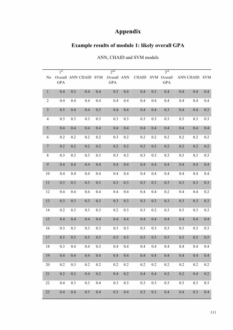
111
Appendix
Example results of module 1: likely overall GPA
ANN, CHAID and SVM models
No 1st
Overall GPA
ANN CHAID SVM 2nd
Overall GPA
ANN CHAID SVM 3rd
Overall GPA
ANN CHAID SVM
1 0.4 0.3 0.4 0.4 0.3 0.4 0.4 0.3 0.4 0.4 0.4 0.4
2 0.4 0.4 0.4 0.4 0.4 0.4 0.4 0.4 0.4 0.4 0.4 0.4
3 0.5 0.4 0.4 0.5 0.4 0.4 0.4 0.4 0.3 0.4 0.4 0.3
4 0.3 0.3 0.3 0.3 0.3 0.3 0.3 0.3 0.3 0.3 0.3 0.3
5 0.4 0.4 0.4 0.4 0.4 0.4 0.4 0.4 0.4 0.4 0.4 0.4
6 0.2 0.2 0.2 0.2 0.3 0.2 0.2 0.2 0.2 0.2 0.2 0.2
7 0.2 0.2 0.2 0.2 0.2 0.2 0.2 0.2 0.2 0.2 0.2 0.2
8 0.3 0.3 0.3 0.3 0.3 0.3 0.3 0.3 0.3 0.3 0.3 0.3
9 0.4 0.4 0.4 0.4 0.4 0.4 0.4 0.4 0.4 0.4 0.4 0.4
10 0.4 0.4 0.4 0.4 0.4 0.4 0.4 0.4 0.4 0.4 0.4 0.4
11 0.3 0.3 0.3 0.3 0.3 0.3 0.3 0.3 0.3 0.3 0.3 0.3
12 0.4 0.4 0.4 0.4 0.4 0.4 0.4 0.4 0.2 0.4 0.4 0.2
13 0.3 0.3 0.3 0.3 0.3 0.3 0.3 0.3 0.3 0.3 0.3 0.3
14 0.2 0.3 0.3 0.3 0.2 0.3 0.3 0.2 0.3 0.3 0.3 0.3
15 0.4 0.4 0.4 0.4 0.4 0.4 0.4 0.4 0.4 0.4 0.4 0.4
16 0.3 0.3 0.3 0.3 0.3 0.3 0.3 0.3 0.3 0.3 0.3 0.3
17 0.5 0.5 0.5 0.5 0.5 0.5 0.5 0.5 0.5 0.5 0.5 0.5
18 0.3 0.4 0.4 0.3 0.4 0.4 0.4 0.4 0.4 0.4 0.4 0.4
19 0.4 0.4 0.4 0.4 0.4 0.4 0.4 0.4 0.4 0.4 0.4 0.4
20 0.2 0.3 0.2 0.2 0.2 0.2 0.2 0.2 0.2 0.2 0.2 0.2
21 0.2 0.2 0.4 0.2 0.4 0.2 0.4 0.4 0.2 0.2 0.4 0.2
22 0.4 0.3 0.3 0.4 0.3 0.3 0.3 0.3 0.3 0.3 0.3 0.3
23 0.4 0.4 0.3 0.4 0.3 0.4 0.3 0.3 0.4 0.4 0.3 0.4

112
24 0.4 0.4 0.3 0.4 0.3 0.4 0.3 0.3 0.3 0.3 0.4 0.3
25 0.3 0.3 0.3 0.3 0.3 0.3 0.3 0.3 0.5 0.5 0.3 0.5
26 0.3 0.3 0.3 0.3 0.3 0.3 0.3 0.3 0.3 0.3 0.3 0.3
27 0.3 0.3 0.3 0.3 0.3 0.3 0.3 0.3 0.3 0.3 0.3 0.3
28 0.3 0.3 0.3 0.3 0.3 0.3 0.3 0.3 0.3 0.3 0.3 0.3
29 0.3 0.3 0.3 0.3 0.3 0.3 0.3 0.3 0.3 0.3 0.3 0.3
30 0.2 0.3 0.2 0.2 0.2 0.3 0.2 0.2 0.3 0.3 0.2 0.3
31 0.5 0.5 0.5 0.5 0.5 0.5 0.5 0.5 0.5 0.5 0.5 0.5
32 0.4 0.4 0.4 0.4 0.4 0.4 0.4 0.4 0.4 0.4 0.4 0.4
33 0.4 0.4 0.4 0.4 0.4 0.4 0.4 0.4 0.4 0.4 0.4 0.4
34 0.3 0.3 0.3 0.3 0.4 0.3 0.3 0.4 0.3 0.3 0.3 0.3
35 0.5 0.5 0.5 0.5 0.5 0.5 0.5 0.5 0.5 0.5 0.5 0.5
36 0.4 0.4 0.4 0.4 0.4 0.4 0.4 0.4 0.4 0.4 0.4 0.4
37 0.3 0.4 0.4 0.3 0.4 0.4 0.4 0.4 0.4 0.4 0.4 0.4
38 0.4 0.4 0.4 0.4 0.4 0.4 0.4 0.4 0.4 0.4 0.4 0.4
39 0.5 0.5 0.5 0.5 0.5 0.5 0.5 0.5 0.5 0.5 0.5 0.5
40 0.6 0.5 0.5 0.6 0.5 0.5 0.5 0.5 0.6 0.6 0.5 0.6
41 0.4 0.3 0.3 0.3 0.3 0.5 0.3 0.3 0.2 0.2 0.3 0.2
42 0.5 0.5 0.4 0.5 0.4 0.5 0.4 0.4 0.5 0.5 0.4 0.5
43 0.3 0.3 0.3 0.3 0.3 0.3 0.3 0.3 0.2 0.2 0.3 0.2
44 0.3 0.3 0.3 0.3 0.3 0.3 0.3 0.3 0.3 0.3 0.3 0.3
45 0.6 0.5 0.4 0.6 0.4 0.4 0.4 0.4 0.4 0.4 0.4 0.4
46 0.3 0.3 0.3 0.3 0.3 0.3 0.3 0.3 0.3 0.3 0.3 0.3
47 0.2 0.2 0.3 0.2 0.2 0.3 0.3 0.2 0.3 0.3 0.3 0.3
48 0.5 0.1 0.4 0.5 0.4 0.5 0.4 0.4 0.5 0.5 0.4 0.5
49 0.3 0.3 0.3 0.3 0.3 0.3 0.3 0.3 0.2 0.2 0.3 0.2
50 0.4 0.4 0.4 0.4 0.4 0.4 0.4 0.4 0.4 0.4 0.4 0.4
51 0.2 0.3 0.3 0.2 0.3 0.3 0.3 0.3 0.3 0.3 0.3 0.3
52 0.4 0.4 0.4 0.4 0.4 0.4 0.4 0.4 0.4 0.4 0.4 0.4
53 0.5 0.5 0.5 0.5 0.5 0.5 0.5 0.5 0.6 0.6 0.5 0.6

113
54 0.2 0.3 0.3 0.2 0.3 0.3 0.3 0.3 0.3 0.3 0.3 0.3
55 0.3 0.3 0.3 0.3 0.3 0.3 0.3 0.3 0.4 0.3 0.3 0.4
56 0.2 0.2 0.2 0.2 0.2 0.2 0.2 0.2 0.2 0.2 0.2 0.2
57 0.4 0.4 0.4 0.4 0.4 0.4 0.4 0.4 0.4 0.4 0.4 0.4
58 0.5 0.5 0.5 0.5 0.5 0.5 0.5 0.5 0.5 0.5 0.5 0.5
59 0.3 0.3 0.3 0.3 0.3 0.3 0.3 0.3 0.3 0.3 0.3 0.3
60 0.5 0.5 0.5 0.5 0.5 0.5 0.5 0.5 0.5 0.5 0.5 0.5
61 0.5 0.5 0.5 0.5 0.5 0.5 0.5 0.5 0.5 0.5 0.5 0.5
62 0.4 0.4 0.4 0.4 0.4 0.4 0.4 0.4 0.4 0.4 0.4 0.4
63 0.5 0.5 0.5 0.5 0.5 0.5 0.5 0.5 0.5 0.5 0.5 0.5
64 0.5 0.5 0.5 0.5 0.5 0.5 0.5 0.5 0.5 0.5 0.5 0.5
65 0.5 0.5 0.5 0.5 0.5 0.5 0.5 0.5 0.5 0.5 0.5 0.5
66 0.3 0.3 0.3 0.3 0.3 0.3 0.3 0.3 0.3 0.3 0.3 0.3
67 0.6 0.5 0.6 0.6 0.4 0.6 0.6 0.4 0.6 0.6 0.6 0.6
68 0.4 0.4 0.4 0.4 0.4 0.4 0.4 0.4 0.4 0.4 0.4 0.4
69 0.4 0.4 0.4 0.4 0.4 0.4 0.4 0.4 0.4 0.4 0.4 0.4
70 0.4 0.4 0.4 0.4 0.4 0.4 0.4 0.4 0.4 0.4 0.4 0.4
71 0.5 0.5 0.5 0.5 0.5 0.5 0.5 0.5 0.5 0.5 0.5 0.5
72 0.3 0.3 0.3 0.3 0.3 0.3 0.3 0.3 0.3 0.3 0.3 0.3
73 0.4 0.4 0.4 0.4 0.4 0.4 0.4 0.4 0.4 0.4 0.4 0.4
74 0.3 0.3 0.3 0.3 0.3 0.3 0.3 0.3 0.3 0.3 0.3 0.3
75 0.2 0.3 0.3 0.2 0.3 0.3 0.3 0.3 0.3 0.3 0.3 0.3
76 0.3 0.3 0.3 0.3 0.3 0.3 0.3 0.3 0.3 0.3 0.3 0.3
77 0.5 0.5 0.5 0.5 0.5 0.5 0.5 0.5 0.5 0.5 0.5 0.5
78 0.4 0.4 0.4 0.4 0.4 0.4 0.4 0.4 0.4 0.4 0.4 0.4
79 0.5 0.5 0.5 0.5 0.5 0.5 0.5 0.5 0.5 0.5 0.5 0.5
80 0.4 0.4 0.4 0.4 0.4 0.4 0.4 0.4 0.4 0.4 0.4 0.4

114
ANN, CHAID and ensemble models
No
1st Overall
GPA
Ens ANN CHD
2nd Overall
GPA
Ens ANN CHD
3rd Overall
GPA
Ens ANN CHD
1 0.4 0.4 0.4 0.4 0.4 0.4 0.4 0.4 0.4 0.4 0.4 0.4
2 0.4 0.4 0.4 0.4 0.4 0.4 0.4 0.4 0.4 0.4 0.4 0.4
3 0.5 0.3 0.4 0.4 0.5 0.4 0.4 0.4 0.5 0.4 0.4 0.4
4 0.2 0.2 0.2 0.2 0.2 0.2 0.2 0.2 0.2 0.2 0.2 0.2
5 0.3 0.3 0.3 0.3 0.3 0.3 0.3 0.3 0.3 0.3 0.3 0.3
6 0.5 0.5 0.5 0.5 0.5 0.5 0.5 0.5 0.5 0.5 0.5 0.5
7 0.4 0.4 0.4 0.4 0.4 0.4 0.4 0.4 0.4 0.4 0.4 0.4
8 0.4 0.4 0.4 0.4 0.4 0.4 0.4 0.4 0.4 0.4 0.4 0.4
9 0.4 0.4 0.4 0.4 0.4 0.4 0.4 0.4 0.4 0.4 0.4 0.4
10 0.1 0.2 0.2 0.2 0.1 0.2 0.2 0.2 0.1 0.2 0.2 0.2
11 0.4 0.4 0.4 0.4 0.4 0.4 0.4 0.4 0.4 0.4 0.4 0.4
12 0.4 0.4 0.4 0.4 0.4 0.4 0.4 0.4 0.4 0.4 0.4 0.4
13 0.4 0.4 0.4 0.4 0.4 0.4 0.4 0.4 0.4 0.4 0.4 0.4
14 0.3 0.3 0.3 0.3 0.3 0.3 0.3 0.3 0.3 0.3 0.3 0.3
15 0.4 0.4 0.4 0.4 0.4 0.4 0.4 0.4 0.4 0.4 0.4 0.4
16 0.2 0.2 0.2 0.4 0.2 0.2 0.2 0.4 0.2 0.2 0.2 0.4
17 0.3 0.3 0.3 0.2 0.3 0.2 0.3 0.2 0.3 0.2 0.3 0.2
18 0.2 0.2 0.3 0.2 0.2 0.2 0.3 0.2 0.2 0.2 0.3 0.2
19 0.2 0.2 0.2 0.2 0.2 0.2 0.2 0.2 0.2 0.2 0.2 0.2
20 0.3 0.3 0.3 0.3 0.3 0.3 0.3 0.3 0.3 0.3 0.3 0.3
21 0.4 0.3 0.3 0.3 0.4 0.3 0.3 0.3 0.4 0.3 0.3 0.3
22 0.2 0.3 0.3 0.3 0.2 0.3 0.3 0.3 0.2 0.3 0.3 0.3
23 0.4 0.3 0.4 0.3 0.4 0.3 0.4 0.3 0.4 0.3 0.4 0.3
24 0.4 0.3 0.4 0.3 0.4 0.3 0.4 0.3 0.4 0.3 0.4 0.3
25 0.3 0.3 0.3 0.3 0.3 0.3 0.3 0.3 0.3 0.3 0.3 0.3

115
26 0.2 0.2 0.2 0.2 0.2 0.2 0.2 0.2 0.2 0.2 0.2 0.2
27 0.3 0.4 0.4 0.4 0.3 0.4 0.4 0.4 0.3 0.4 0.4 0.4
28 0.3 0.3 0.3 0.3 0.3 0.3 0.3 0.3 0.3 0.3 0.3 0.3
29 0.1 0.2 0.2 0.2 0.1 0.2 0.2 0.2 0.1 0.2 0.2 0.2
30 0.3 0.3 0.3 0.3 0.3 0.3 0.3 0.3 0.3 0.3 0.3 0.3
31 0.4 0.3 0.3 0.3 0.4 0.3 0.3 0.3 0.4 0.3 0.3 0.3
32 0.4 0.4 0.4 0.4 0.4 0.4 0.4 0.4 0.4 0.4 0.4 0.4
33 0.2 0.2 0.2 0.2 0.2 0.2 0.2 0.2 0.2 0.2 0.2 0.2
34 0.4 0.3 0.3 0.3 0.4 0.3 0.3 0.3 0.4 0.3 0.3 0.3
35 0.2 0.2 0.2 0.2 0.2 0.2 0.2 0.2 0.2 0.2 0.2 0.2
36 0.4 0.5 0.5 0.4 0.4 0.4 0.5 0.4 0.4 0.4 0.5 0.4
37 0.4 0.3 0.3 0.3 0.4 0.3 0.3 0.3 0.4 0.3 0.3 0.3
38 0.4 0.4 0.4 0.4 0.4 0.4 0.4 0.4 0.4 0.4 0.4 0.4
39 0.3 0.4 0.4 0.4 0.3 0.4 0.4 0.4 0.3 0.4 0.4 0.4
40 0.2 0.2 0.2 0.2 0.2 0.2 0.2 0.2 0.2 0.2 0.2 0.2
41 0.5 0.5 0.5 0.4 0.5 0.4 0.5 0.4 0.5 0.4 0.5 0.4
42 0.3 0.3 0.3 0.3 0.3 0.3 0.3 0.3 0.3 0.3 0.3 0.3
43 0.4 0.4 0.4 0.4 0.4 0.4 0.4 0.4 0.4 0.4 0.4 0.4
44 0.4 0.4 0.4 0.4 0.4 0.4 0.4 0.4 0.4 0.4 0.4 0.4
45 0.2 0.2 0.2 0.2 0.2 0.2 0.2 0.2 0.2 0.2 0.2 0.2
46 0.5 0.4 0.5 0.4 0.5 0.4 0.5 0.4 0.5 0.4 0.5 0.4
47 0.3 0.3 0.3 0.3 0.3 0.3 0.3 0.3 0.3 0.3 0.3 0.3
48 0.3 0.4 0.4 0.4 0.3 0.4 0.4 0.4 0.3 0.4 0.4 0.4
49 0.5 0.4 0.4 0.4 0.5 0.4 0.4 0.4 0.5 0.4 0.4 0.4
50 0.5 0.5 0.5 0.5 0.5 0.5 0.5 0.5 0.5 0.5 0.5 0.5
* Please note that “Ens” is ensemble and “CHD” is CHAID algorithm

116
Results of the MANN-OWSR, SVM and ensemble in overall GPA and GPA each semester
No. 1st
Overall GPA
SVM OWSR Ensemble 2nd
Overall GPA
SVM OWSR Ensemble 3rd
Overall GPA
SVM OWSR Ensemble
1 0.4 0.4 0.4 0.4 0.3 0.3 0.3 0.3 0.4 0.4 0.4 0.4
2 0.4 0.4 0.4 0.4 0.3 0.3 0.3 0.3 0.4 0.4 0.4 0.4
3 0.3 0.3 0.3 0.3 0.2 0.2 0.2 0.2 0.5 0.5 0.5 0.4
4 0.2 0.2 0.2 0.2 0.5 0.5 0.5 0.5 0.2 0.2 0.2 0.2
5 0.3 0.3 0.3 0.3 0.4 0.4 0.4 0.4 0.3 0.3 0.3 0.3
6 0.3 0.3 0.3 0.3 0.3 0.3 0.3 0.3 0.5 0.5 0.5 0.5
7 0.4 0.4 0.4 0.4 0.2 0.2 0.2 0.2 0.4 0.4 0.4 0.4
8 0.3 0.3 0.3 0.3 0.3 0.3 0.3 0.3 0.4 0.4 0.4 0.4
9 0.3 0.3 0.3 0.3 0.4 0.4 0.4 0.4 0.4 0.4 0.4 0.4
10 0.3 0.3 0.3 0.3 0.3 0.3 0.3 0.4 0.1 0.1 0.1 0.2
11 0.4 0.4 0.4 0.4 0.6 0.6 0.6 0.5 0.4 0.4 0.4 0.4
12 0.4 0.4 0.4 0.4 0.3 0.3 0.3 0.3 0.4 0.4 0.4 0.4
13 0.3 0.3 0.3 0.3 0.3 0.3 0.3 0.3 0.4 0.4 0.4 0.4
14 0.4 0.4 0.4 0.4 0.3 0.3 0.3 0.3 0.3 0.3 0.3 0.3
15 0.4 0.4 0.4 0.4 0.4 0.4 0.4 0.4 0.4 0.4 0.4 0.4
16 0.5 0.5 0.5 0.5 0.3 0.3 0.3 0.3 0.2 0.2 0.2 0.2
17 0.2 0.2 0.2 0.2 0.2 0.2 0.2 0.3 0.3 0.3 0.3 0.3
18 0.5 0.5 0.5 0.5 0.2 0.2 0.2 0.3 0.2 0.2 0.2 0.2
19 0.2 0.2 0.2 0.2 0.5 0.5 0.5 0.5 0.2 0.2 0.2 0.2
20 0.3 0.3 0.3 0.3 0.4 0.4 0.4 0.4 0.3 0.3 0.3 0.3
21 0.3 0.3 0.3 0.3 0.4 0.4 0.4 0.4 0.4 0.4 0.4 0.3
22 0.4 0.4 0.4 0.4 0.3 0.3 0.3 0.3 0.2 0.2 0.2 0.3
23 0.2 0.2 0.2 0.2 0.2 0.2 0.2 0.2 0.4 0.4 0.4 0.3
24 0.2 0.2 0.2 0.2 0.2 0.2 0.2 0.2 0.4 0.4 0.4 0.4
25 0.2 0.2 0.2 0.2 0.3 0.3 0.3 0.3 0.3 0.3 0.3 0.3

117
26 0.2 0.2 0.2 0.3 0.3 0.3 0.3 0.3 0.2 0.2 0.2 0.2
27 0.5 0.5 0.5 0.5 0.3 0.3 0.3 0.3 0.3 0.3 0.3 0.4
28 0.4 0.4 0.4 0.4 0.2 0.2 0.2 0.3 0.3 0.3 0.3 0.3
29 0.4 0.4 0.4 0.4 0.4 0.4 0.4 0.4 0.1 0.1 0.1 0.2
30 0.3 0.3 0.3 0.3 0.5 0.5 0.5 0.5 0.3 0.3 0.3 0.3
31 0.3 0.3 0.3 0.3 0.3 0.3 0.3 0.3 0.4 0.4 0.4 0.3
32 0.2 0.2 0.2 0.2 0.3 0.3 0.3 0.3 0.4 0.4 0.4 0.4
33 0.3 0.3 0.3 0.3 0.3 0.3 0.3 0.3 0.2 0.2 0.2 0.2
34 0.3 0.3 0.3 0.3 0.2 0.2 0.2 0.2 0.4 0.4 0.4 0.3
35 0.6 0.6 0.6 0.3 0.2 0.2 0.2 0.3 0.2 0.2 0.2 0.2
36 0.3 0.3 0.3 0.3 0.3 0.3 0.3 0.3 0.4 0.4 0.4 0.4
37 0.3 0.3 0.3 0.4 0.4 0.4 0.4 0.3 0.4 0.4 0.4 0.3
38 0.2 0.2 0.2 0.2 0.4 0.4 0.4 0.4 0.4 0.4 0.4 0.4
39 0.3 0.3 0.3 0.3 0.4 0.4 0.4 0.4 0.3 0.3 0.3 0.4
40 0.2 0.2 0.2 0.2 0.2 0.2 0.2 0.2 0.2 0.2 0.2 0.2
41 0.3 0.3 0.3 0.3 0.2 0.2 0.2 0.2 0.5 0.5 0.5 0.4
42 0.3 0.3 0.3 0.3 0.4 0.4 0.4 0.3 0.3 0.3 0.3 0.3
43 0.2 0.2 0.2 0.2 0.2 0.2 0.2 0.2 0.4 0.4 0.4 0.4
44 0.4 0.4 0.4 0.3 0.5 0.5 0.5 0.5 0.4 0.3 0.4 0.4
45 0.5 0.5 0.5 0.5 0.2 0.2 0.2 0.2 0.2 0.2 0.2 0.2
46 0.2 0.2 0.2 0.2 0.3 0.3 0.3 0.3 0.5 0.5 0.5 0.5
47 0.3 0.3 0.3 0.3 0.3 0.3 0.3 0.3 0.3 0.3 0.3 0.3
48 0.3 0.3 0.3 0.3 0.4 0.4 0.4 0.4 0.3 0.3 0.4 0.4
49 0.5 0.5 0.5 0.5 0.2 0.2 0.2 0.2 0.5 0.5 0.5 0.4
50 0.3 0.3 0.3 0.3 0.2 0.2 0.2 0.2 0.5 0.5 0.5 0.5

118
Example results of module 2: ranked programme recommendation
Association Rules (GRI) models
No 1st
Ranking GRI
2nd
Ranking GRI
3rd
Ranking GRI
1 0.4 0.4 0.1 0.1 0.5 0.5
2 0.3 0.2 0.6 0.6 0.1 0.3
3 0.6 0.3 0.4 0.4 0.5 0.5
4 0.4 0.2 0.1 0.1 0.5 0.5
5 0.4 0.2 0.1 0.5 0.1 0.1
6 0.3 0.2 0.6 0.2 0.5 0.5
7 0.3 0.4 0.2 0.5 0.5 0.5
8 0.2 0.2 0.2 0.2 0.5 0.5
9 0.5 0.4 0.5 0.5 0.5 0.5
10 0.2 0.2 0.5 0.5 0.5 0.5
11 0.4 0.2 0.5 0.5 0.4 0.4
12 0.4 0.5 0.5 0.4 0.5 0.5
13 0.2 0.5 0.5 0.5 0.4 0.4
14 0.2 0.2 0.5 0.5 0.4 0.4
15 0.2 0.2 0.4 0.4 0.3 0.3
16 0.4 0.5 0.5 0.5 0.5 0.5
17 0.4 0.5 0.5 0.5 0.5 0.5
18 0.4 0.1 0.3 0.3 0.5 0.5
19 0.2 0.2 0.1 0.4 0.3 0.3
20 0.3 0.3 0.4 0.4 0.5 0.5
21 0.3 0.3 0.1 0.2 0.5 0.5
22 0.4 0.4 0.5 0.5 0.5 0.5
23 0.2 0.1 0.1 0.5 0.5 0.5
24 0.4 0.4 0.1 0.5 0.3 0.7

119
25 0.2 0.2 0.4 0.4 0.7 0.7
26 0.3 0.3 0.5 0.5 0.5 0.5
27 0.4 0.4 0.6 0.6 0.5 0.5
28 0.5 0.5 0.5 0.5 0.5 0.5
29 0.4 0.4 0.5 0.5 0.5 0.5
30 0.5 0.5 0.2 0.2 0.5 0.5
31 0.3 0.3 0.2 0.2 0.5 0.5
32 0.4 0.4 0.4 0.4 0.5 0.5
33 0.4 0.4 0.5 0.5 0.5 0.5
34 0.3 0.3 0.7 0.5 0.5 0.5
35 0.4 0.4 0.5 0.5 0.5 0.5
36 0.5 0.1 0.7 0.5 0.5 0.5
37 0.5 0.5 0.5 0.5 0.5 0.5
38 0.2 0.2 0.5 0.5 0.3 0.5
39 0.3 0.3 0.3 0.3 0.5 0.5
40 0.5 0.5 0.3 0.3 0.5 0.5
41 0.3 0.3 0.3 0.3 0.3 0.3
42 0.5 0.5 0.6 0.6 0.6 0.6
43 0.3 0.3 0.6 0.5 0.5 0.5
44 0.2 0.2 0.5 0.5 0.5 0.5
45 0.4 0.1 0.6 0.5 0.5 0.5
46 0.5 0.5 0.5 0.5 0.5 0.5
47 0.4 0.4 0.6 0.6 0.6 0.6
48 0.3 0.4 0.4 0.4 0.5 0.5
49 0.3 0.3 0.6 0.6 0.6 0.6
50 0.3 0.3 0.6 0.5 0.7 0.7
51 0.2 0.2 0.5 0.5 0.7 0.7
52 0.4 0.4 0.2 0.2 0.5 0.5
53 0.4 0.4 0.4 0.4 0.5 0.5
54 0.4 0.4 0.6 0.6 0.7 0.6

120
55 0.5 0.1 0.7 0.5 0.5 0.5
56 0.4 0.4 0.5 0.4 0.7 0.5
57 0.4 0.4 0.5 0.1 0.7 0.5
58 0.3 0.3 0.7 0.5 0.5 0.5
59 0.3 0.3 0.7 0.2 0.5 0.5
60 0.3 0.3 0.5 0.5 0.1 0.1
61 0.4 0.4 0.5 0.2 0.1 0.3
62 0.3 0.3 0.5 0.5 0.1 0.1
63 0.4 0.4 0.5 0.5 0.1 0.5
64 0.4 0.4 0.5 0.5 0.1 0.5
65 0.4 0.4 0.5 0.4 0.5 0.5
66 0.3 0.1 0.6 0.5 0.5 0.1
67 0.4 0.4 0.5 0.5 0.5 0.1
68 0.4 0.4 0.2 0.2 0.5 0.5
69 0.5 0.5 0.5 0.5 0.5 0.2
70 0.5 0.5 0.5 0.5 0.3 0.3
Example results of module 3: likely GPA for each semester
Semester 1 of year 1
ANN, CHAID and SVM models
No. 1st
GPA Y1S1
ANN CHD SVM 2nd
GPA Y1S1
ANN CHD SVM 3rd
GPA Y1S1
ANN CHD SVM
1 0.3 0.2 0.2 0.3 0.4 0.4 0.4 0.4 0.3 0.3 0.3 0.3
2 0.1 0.3 0.2 0.1 0.3 0.3 0.3 0.3 0.4 0.4 0.4 0.4
3 0.3 0.3 0.2 0.3 0.3 0.3 0.3 0.3 0.3 0.3 0.3 0.3
4 0.3 0.3 0.2 0.3 0.4 0.3 0.3 0.4 0.5 0.4 0.5 0.5
5 0.3 0.4 0.4 0.3 0.4 0.3 0.3 0.4 0.5 0.4 0.5 0.5

121
6 0.2 0.2 0.3 0.2 0.5 0.4 0.4 0.5 0.4 0.3 0.4 0.4
7 0.3 0.4 0.3 0.3 0.3 0.4 0.4 0.3 0.2 0.3 0.3 0.2
8 0.4 0.4 0.4 0.4 0.4 0.4 0.4 0.4 0.2 0.3 0.3 0.2
9 0.3 0.4 0.3 0.3 0.4 0.4 0.4 0.4 0.3 0.3 0.3 0.3
10 0.3 0.3 0.3 0.3 0.3 0.3 0.3 0.3 0.4 0.4 0.4 0.4
11 0.4 0.4 0.3 0.4 0.2 0.3 0.2 0.2 0.4 0.4 0.4 0.4
12 0.5 0.4 0.3 0.5 0.3 0.3 0.3 0.3 0.3 0.3 0.3 0.3
13 0.3 0.4 0.4 0.3 0.3 0.3 0.3 0.3 0.3 0.4 0.3 0.3
14 0.5 0.5 0.4 0.5 0.4 0.4 0.4 0.4 0.4 0.3 0.3 0.4
15 0.4 0.3 0.3 0.4 0.4 0.4 0.4 0.4 0.3 0.3 0.3 0.3
16 0.3 0.4 0.3 0.3 0.4 0.3 0.3 0.4 0.5 0.4 0.4 0.5
17 0.2 0.3 0.2 0.2 0.4 0.3 0.3 0.4 0.3 0.4 0.4 0.3
18 0.2 0.3 0.3 0.2 0.3 0.3 0.3 0.3 0.5 0.4 0.4 0.5
19 0.4 0.5 0.4 0.4 0.3 0.3 0.3 0.3 0.3 0.3 0.3 0.3
20 0.2 0.3 0.3 0.2 0.5 0.5 0.4 0.5 0.4 0.4 0.4 0.4
21 0.5 0.5 0.5 0.5 0.3 0.3 0.3 0.3 0.2 0.3 0.2 0.2
22 0.4 0.4 0.4 0.4 0.3 0.3 0.3 0.3 0.3 0.4 0.3 0.3
23 0.4 0.4 0.4 0.4 0.3 0.3 0.3 0.3 0.2 0.3 0.3 0.2
24 0.4 0.4 0.4 0.4 0.4 0.3 0.3 0.4 0.4 0.4 0.4 0.4
25 0.4 0.5 0.5 0.4 0.4 0.5 0.4 0.4 0.3 0.3 0.3 0.3
26 0.4 0.3 0.3 0.4 0.3 0.4 0.4 0.3 0.3 0.3 0.3 0.3
27 0.4 0.4 0.4 0.4 0.4 0.3 0.3 0.4 0.3 0.3 0.2 0.3
28 0.5 0.5 0.5 0.5 0.4 0.5 0.4 0.4 0.3 0.2 0.2 0.3
29 0.3 0.3 0.3 0.3 0.5 0.5 0.5 0.5 0.3 0.3 0.3 0.3
30 0.4 0.4 0.4 0.4 0.2 0.3 0.2 0.2 0.3 0.3 0.3 0.3
31 0.3 0.4 0.3 0.3 0.4 0.4 0.4 0.4 0.3 0.3 0.2 0.3
32 0.4 0.3 0.3 0.4 0.4 0.3 0.3 0.4 0.3 0.3 0.3 0.3
33 0.2 0.3 0.2 0.2 0.3 0.3 0.3 0.3 0.4 0.3 0.3 0.4
34 0.4 0.4 0.4 0.4 0.4 0.5 0.4 0.4 0.4 0.4 0.4 0.4
35 0.3 0.3 0.3 0.3 0.4 0.4 0.4 0.4 0.5 0.4 0.3 0.5

122
36 0.4 0.3 0.3 0.4 0.3 0.3 0.2 0.3 0.4 0.3 0.3 0.4
37 0.4 0.3 0.3 0.4 0.4 0.4 0.4 0.4 0.5 0.4 0.4 0.5
38 0.3 0.3 0.3 0.3 0.5 0.5 0.5 0.5 0.2 0.3 0.3 0.2
39 0.4 0.5 0.3 0.4 0.2 0.2 0.2 0.2 0.4 0.4 0.5 0.4
40 0.5 0.5 0.4 0.5 0.3 0.2 0.2 0.3 0.2 0.3 0.3 0.2
41 0.3 0.3 0.3 0.3 0.5 0.3 0.3 0.5 0.2 0.3 0.2 0.2
42 0.4 0.5 0.5 0.4 0.3 0.3 0.3 0.3 0.4 0.3 0.3 0.4
43 0.3 0.4 0.4 0.3 0.4 0.3 0.4 0.4 0.2 0.3 0.3 0.2
44 0.4 0.4 0.4 0.4 0.3 0.3 0.3 0.3 0.5 0.4 0.4 0.5
45 0.2 0.3 0.2 0.2 0.5 0.5 0.4 0.5 0.3 0.3 0.3 0.3
46 0.4 0.4 0.3 0.4 0.5 0.5 0.3 0.5 0.4 0.3 0.3 0.4
47 0.3 0.3 0.3 0.3 0.3 0.3 0.3 0.3 0.4 0.4 0.4 0.4
48 0.3 0.3 0.3 0.3 0.4 0.5 0.4 0.4 0.3 0.4 0.4 0.3
49 0.4 0.3 0.3 0.4 0.4 0.3 0.3 0.4 0.4 0.3 0.3 0.4
50 0.2 0.2 0.3 0.2 0.2 0.2 0.3 0.2 0.5 0.4 0.4 0.5
ANN, CHAID and ensemble models
No.
1st
GPA
Y1S1
ANN CHD Ens 2nd
GPA Y1S1
ANN CHD Ens
3rd
GPA
Y1S1
ANN CHD Ens
1 0.3 0.2 0.2 0.2 0.4 0.4 0.4 0.4 0.3 0.3 0.3 0.3
2 0.1 0.3 0.2 0.2 0.3 0.3 0.3 0.3 0.4 0.4 0.4 0.4
3 0.3 0.3 0.2 0.3 0.3 0.3 0.3 0.3 0.3 0.3 0.3 0.3
4 0.3 0.3 0.2 0.3 0.4 0.3 0.3 0.3 0.5 0.4 0.5 0.5
5 0.3 0.4 0.4 0.4 0.4 0.3 0.3 0.3 0.5 0.4 0.5 0.5
6 0.2 0.2 0.3 0.2 0.5 0.4 0.4 0.4 0.4 0.3 0.4 0.4
7 0.3 0.4 0.3 0.3 0.3 0.4 0.4 0.4 0.2 0.3 0.3 0.3
8 0.4 0.4 0.4 0.4 0.4 0.4 0.4 0.4 0.2 0.3 0.3 0.3

123
9 0.3 0.4 0.3 0.3 0.4 0.4 0.4 0.4 0.3 0.3 0.3 0.3
10 0.3 0.3 0.3 0.3 0.3 0.3 0.3 0.3 0.4 0.4 0.4 0.4
11 0.4 0.4 0.3 0.3 0.2 0.3 0.2 0.2 0.4 0.4 0.4 0.4
12 0.5 0.4 0.3 0.3 0.3 0.3 0.3 0.3 0.3 0.3 0.3 0.3
13 0.3 0.4 0.4 0.4 0.3 0.3 0.3 0.3 0.3 0.4 0.3 0.3
14 0.5 0.5 0.4 0.5 0.4 0.4 0.4 0.4 0.4 0.3 0.3 0.3
15 0.4 0.3 0.3 0.3 0.4 0.4 0.4 0.4 0.3 0.3 0.3 0.3
16 0.3 0.4 0.3 0.3 0.4 0.3 0.3 0.3 0.5 0.4 0.4 0.4
17 0.2 0.3 0.2 0.2 0.4 0.3 0.3 0.3 0.3 0.4 0.4 0.4
18 0.2 0.3 0.3 0.3 0.3 0.3 0.3 0.3 0.5 0.4 0.4 0.4
19 0.4 0.5 0.4 0.4 0.3 0.3 0.3 0.3 0.3 0.3 0.3 0.3
20 0.2 0.3 0.3 0.3 0.5 0.5 0.4 0.5 0.4 0.4 0.4 0.4
21 0.5 0.5 0.5 0.5 0.3 0.3 0.3 0.3 0.2 0.3 0.2 0.2
22 0.4 0.4 0.4 0.4 0.3 0.3 0.3 0.3 0.3 0.4 0.3 0.3
23 0.4 0.4 0.4 0.4 0.3 0.3 0.3 0.3 0.2 0.3 0.3 0.3
24 0.4 0.4 0.4 0.4 0.4 0.3 0.3 0.3 0.4 0.4 0.4 0.4
25 0.4 0.5 0.5 0.5 0.4 0.5 0.4 0.4 0.3 0.3 0.3 0.3
26 0.4 0.3 0.3 0.3 0.3 0.4 0.4 0.4 0.3 0.3 0.3 0.3
27 0.4 0.4 0.4 0.4 0.4 0.3 0.3 0.3 0.3 0.3 0.2 0.2
28 0.5 0.5 0.5 0.5 0.4 0.5 0.4 0.4 0.3 0.2 0.2 0.2
29 0.3 0.3 0.3 0.3 0.5 0.5 0.5 0.5 0.3 0.3 0.3 0.3
30 0.4 0.4 0.4 0.4 0.2 0.3 0.2 0.2 0.3 0.3 0.3 0.3
31 0.3 0.4 0.3 0.3 0.4 0.4 0.4 0.4 0.3 0.3 0.2 0.2
32 0.4 0.3 0.3 0.3 0.4 0.3 0.3 0.3 0.3 0.3 0.3 0.3
33 0.2 0.3 0.2 0.2 0.3 0.3 0.3 0.3 0.4 0.3 0.3 0.3
34 0.4 0.4 0.4 0.4 0.4 0.5 0.4 0.4 0.4 0.4 0.4 0.4
35 0.3 0.3 0.3 0.3 0.4 0.4 0.4 0.4 0.5 0.4 0.3 0.3
36 0.4 0.3 0.3 0.3 0.3 0.3 0.2 0.3 0.4 0.3 0.3 0.3
37 0.4 0.3 0.3 0.3 0.4 0.4 0.4 0.4 0.5 0.4 0.4 0.4
38 0.3 0.3 0.3 0.3 0.5 0.5 0.5 0.5 0.2 0.3 0.3 0.3

124
39 0.4 0.5 0.3 0.3 0.2 0.2 0.2 0.2 0.4 0.4 0.5 0.5
40 0.5 0.5 0.4 0.5 0.3 0.2 0.2 0.2 0.2 0.3 0.3 0.3
41 0.3 0.3 0.3 0.3 0.5 0.3 0.3 0.3 0.2 0.3 0.2 0.2
42 0.4 0.5 0.5 0.5 0.3 0.3 0.3 0.3 0.4 0.3 0.3 0.3
43 0.3 0.4 0.4 0.4 0.4 0.3 0.4 0.4 0.2 0.3 0.3 0.3
44 0.4 0.4 0.4 0.4 0.3 0.3 0.3 0.3 0.5 0.4 0.4 0.4
45 0.2 0.3 0.2 0.2 0.5 0.5 0.4 0.5 0.3 0.3 0.3 0.3
46 0.4 0.4 0.3 0.4 0.5 0.5 0.3 0.5 0.4 0.3 0.3 0.3
47 0.3 0.3 0.3 0.3 0.3 0.3 0.3 0.3 0.4 0.4 0.4 0.4
48 0.3 0.3 0.3 0.3 0.4 0.5 0.4 0.4 0.3 0.4 0.4 0.4
49 0.4 0.3 0.3 0.3 0.4 0.3 0.3 0.3 0.4 0.3 0.3 0.3
50 0.2 0.2 0.3 0.2 0.2 0.2 0.3 0.2 0.5 0.4 0.4 0.4
SVM, MANN-OWSR and ensemble models
No.
1st
GPA
Y1S1
SVM OWSR Ens 2nd
GPA Y1S1
SVM OWSR Ens
3rd
GPA
Y1S1
SVM OWSR Ens
1 0.3 0.3 0.3 0.3 0.4 0.4 0.4 0.3 0.2 0.2 0.2 0.3
2 0.4 0.4 0.4 0.4 0.3 0.3 0.3 0.3 0.4 0.4 0.4 0.4
3 0.3 0.3 0.3 0.3 0.3 0.3 0.3 0.3 0.3 0.3 0.3 0.3
4 0.5 0.5 0.5 0.5 0.4 0.3 0.3 0.3 0.5 0.4 0.5 0.5
5 0.5 0.5 0.5 0.5 0.4 0.3 0.3 0.3 0.5 0.4 0.5 0.5
6 0.4 0.4 0.4 0.4 0.5 0.4 0.4 0.4 0.4 0.3 0.4 0.4
7 0.2 0.2 0.2 0.3 0.3 0.4 0.4 0.4 0.2 0.3 0.3 0.3
8 0.2 0.2 0.2 0.3 0.4 0.4 0.4 0.4 0.2 0.3 0.3 0.3
9 0.3 0.3 0.3 0.3 0.4 0.4 0.4 0.4 0.3 0.3 0.3 0.3
10 0.4 0.4 0.4 0.4 0.3 0.3 0.3 0.3 0.4 0.4 0.4 0.4
11 0.4 0.4 0.4 0.4 0.2 0.3 0.2 0.2 0.4 0.4 0.4 0.4

125
12 0.3 0.3 0.3 0.3 0.3 0.3 0.3 0.3 0.3 0.3 0.3 0.3
13 0.3 0.3 0.3 0.3 0.3 0.3 0.3 0.3 0.3 0.4 0.3 0.3
14 0.4 0.4 0.4 0.3 0.4 0.4 0.4 0.4 0.4 0.3 0.3 0.3
15 0.3 0.3 0.3 0.3 0.4 0.4 0.4 0.4 0.3 0.3 0.3 0.3
16 0.5 0.5 0.5 0.4 0.4 0.3 0.3 0.3 0.5 0.4 0.4 0.4
17 0.3 0.3 0.3 0.4 0.4 0.3 0.3 0.3 0.3 0.4 0.4 0.4
18 0.5 0.5 0.5 0.4 0.3 0.3 0.3 0.3 0.5 0.4 0.4 0.4
19 0.3 0.3 0.3 0.3 0.3 0.3 0.3 0.3 0.3 0.3 0.3 0.3
20 0.4 0.4 0.4 0.4 0.5 0.5 0.4 0.5 0.4 0.4 0.4 0.4
21 0.2 0.2 0.2 0.2 0.3 0.3 0.3 0.3 0.2 0.3 0.2 0.2
22 0.3 0.3 0.3 0.3 0.3 0.3 0.3 0.3 0.3 0.4 0.3 0.3
23 0.2 0.2 0.2 0.3 0.3 0.3 0.3 0.3 0.2 0.3 0.3 0.3
24 0.4 0.4 0.4 0.4 0.4 0.3 0.3 0.3 0.4 0.4 0.4 0.4
25 0.3 0.3 0.3 0.3 0.4 0.5 0.4 0.4 0.3 0.3 0.3 0.3
26 0.3 0.3 0.3 0.3 0.3 0.4 0.4 0.4 0.3 0.3 0.3 0.3
27 0.3 0.3 0.3 0.2 0.4 0.3 0.3 0.3 0.3 0.3 0.2 0.2
28 0.3 0.3 0.3 0.2 0.4 0.5 0.4 0.4 0.3 0.2 0.2 0.2
29 0.3 0.3 0.3 0.3 0.5 0.5 0.5 0.5 0.3 0.3 0.3 0.3
30 0.3 0.3 0.3 0.3 0.2 0.3 0.2 0.2 0.3 0.3 0.3 0.3
31 0.3 0.3 0.3 0.2 0.4 0.4 0.4 0.4 0.3 0.3 0.2 0.2
32 0.3 0.3 0.3 0.3 0.4 0.3 0.3 0.3 0.3 0.3 0.3 0.3
33 0.4 0.4 0.4 0.3 0.3 0.3 0.3 0.3 0.4 0.3 0.3 0.3
34 0.4 0.4 0.4 0.4 0.4 0.5 0.4 0.4 0.4 0.4 0.4 0.4
35 0.5 0.5 0.5 0.3 0.4 0.4 0.4 0.4 0.5 0.4 0.3 0.3
36 0.4 0.4 0.4 0.3 0.3 0.3 0.2 0.3 0.4 0.3 0.3 0.3
37 0.5 0.5 0.5 0.4 0.4 0.4 0.4 0.4 0.5 0.4 0.4 0.4
38 0.2 0.2 0.2 0.3 0.5 0.5 0.5 0.5 0.2 0.3 0.3 0.3
39 0.4 0.4 0.4 0.5 0.2 0.2 0.2 0.2 0.4 0.4 0.5 0.5
40 0.2 0.2 0.2 0.3 0.3 0.2 0.2 0.2 0.2 0.3 0.3 0.3
41 0.2 0.2 0.2 0.2 0.5 0.3 0.3 0.3 0.2 0.3 0.2 0.2

126
42 0.4 0.4 0.4 0.3 0.3 0.3 0.3 0.3 0.4 0.3 0.3 0.3
43 0.2 0.2 0.2 0.3 0.4 0.3 0.4 0.4 0.2 0.3 0.3 0.3
44 0.5 0.5 0.5 0.4 0.3 0.3 0.3 0.3 0.5 0.4 0.4 0.4
45 0.3 0.3 0.3 0.3 0.5 0.5 0.4 0.5 0.3 0.3 0.3 0.3
46 0.4 0.4 0.4 0.3 0.5 0.5 0.3 0.5 0.4 0.3 0.3 0.3
47 0.4 0.4 0.4 0.4 0.3 0.3 0.3 0.3 0.4 0.4 0.4 0.4
48 0.3 0.3 0.3 0.4 0.4 0.5 0.4 0.4 0.3 0.4 0.4 0.4
49 0.4 0.4 0.4 0.3 0.4 0.3 0.3 0.3 0.4 0.3 0.3 0.3
50 0.5 0.5 0.5 0.4 0.2 0.2 0.3 0.2 0.5 0.4 0.4 0.4
Semester 2 of year 1
ANN, CHAID and SVM models
No. 1st
GPA Y1S2
ANN CHD SVM 2nd
GPA Y1S2
ANN CHD SVM 3rd
GPA Y1S2
ANN CHD SVM
1 0.3 0.2 0.2 0.3 0.4 0.4 0.4 0.4 0.3 0.3 0.3 0.3
2 0.1 0.3 0.2 0.1 0.3 0.3 0.3 0.3 0.4 0.4 0.4 0.4
3 0.3 0.3 0.2 0.3 0.3 0.3 0.3 0.3 0.3 0.3 0.3 0.3
4 0.3 0.3 0.2 0.3 0.4 0.3 0.3 0.4 0.5 0.4 0.5 0.5
5 0.3 0.4 0.4 0.3 0.4 0.3 0.3 0.4 0.5 0.4 0.5 0.5
6 0.2 0.2 0.3 0.2 0.5 0.4 0.4 0.5 0.4 0.3 0.4 0.4
7 0.3 0.4 0.3 0.3 0.3 0.4 0.4 0.3 0.2 0.3 0.3 0.2
8 0.4 0.4 0.4 0.4 0.4 0.4 0.4 0.4 0.2 0.3 0.3 0.2
9 0.3 0.4 0.3 0.3 0.4 0.4 0.4 0.4 0.3 0.3 0.3 0.3
10 0.3 0.3 0.3 0.3 0.3 0.3 0.3 0.3 0.4 0.4 0.4 0.4
11 0.4 0.4 0.3 0.4 0.2 0.3 0.2 0.2 0.4 0.4 0.4 0.4
12 0.5 0.4 0.3 0.5 0.3 0.3 0.3 0.3 0.3 0.3 0.3 0.3
13 0.3 0.4 0.4 0.3 0.3 0.3 0.3 0.3 0.3 0.4 0.3 0.3
14 0.5 0.5 0.4 0.5 0.4 0.4 0.4 0.4 0.4 0.3 0.3 0.4

127
15 0.4 0.3 0.3 0.4 0.4 0.4 0.4 0.4 0.3 0.3 0.3 0.3
16 0.3 0.4 0.3 0.3 0.4 0.3 0.3 0.4 0.5 0.4 0.4 0.5
17 0.2 0.3 0.2 0.2 0.4 0.3 0.3 0.4 0.3 0.4 0.4 0.3
18 0.2 0.3 0.3 0.2 0.3 0.3 0.3 0.3 0.5 0.4 0.4 0.5
19 0.4 0.5 0.4 0.4 0.3 0.3 0.3 0.3 0.3 0.3 0.3 0.3
20 0.2 0.3 0.3 0.2 0.5 0.5 0.4 0.5 0.4 0.4 0.4 0.4
21 0.5 0.5 0.5 0.5 0.3 0.3 0.3 0.3 0.2 0.3 0.2 0.2
22 0.4 0.4 0.4 0.4 0.3 0.3 0.3 0.3 0.3 0.4 0.3 0.3
23 0.4 0.4 0.4 0.4 0.3 0.3 0.3 0.3 0.2 0.3 0.3 0.2
24 0.4 0.4 0.4 0.4 0.4 0.3 0.3 0.4 0.4 0.4 0.4 0.4
25 0.4 0.5 0.5 0.4 0.4 0.5 0.4 0.4 0.3 0.3 0.3 0.3
26 0.4 0.3 0.3 0.4 0.3 0.4 0.4 0.3 0.3 0.3 0.3 0.3
27 0.4 0.4 0.4 0.4 0.4 0.3 0.3 0.4 0.3 0.3 0.2 0.3
28 0.5 0.5 0.5 0.5 0.4 0.5 0.4 0.4 0.3 0.2 0.2 0.3
29 0.3 0.3 0.3 0.3 0.5 0.5 0.5 0.5 0.3 0.3 0.3 0.3
30 0.4 0.4 0.4 0.4 0.2 0.3 0.2 0.2 0.3 0.3 0.3 0.3
31 0.3 0.4 0.3 0.3 0.4 0.4 0.4 0.4 0.3 0.3 0.2 0.3
32 0.4 0.3 0.3 0.4 0.4 0.3 0.3 0.4 0.3 0.3 0.3 0.3
33 0.2 0.3 0.2 0.2 0.3 0.3 0.3 0.3 0.4 0.3 0.3 0.4
34 0.4 0.4 0.4 0.4 0.4 0.5 0.4 0.4 0.4 0.4 0.4 0.4
35 0.3 0.3 0.3 0.3 0.4 0.4 0.4 0.4 0.5 0.4 0.3 0.5
36 0.4 0.3 0.3 0.4 0.3 0.3 0.2 0.3 0.4 0.3 0.3 0.4
37 0.4 0.3 0.3 0.4 0.4 0.4 0.4 0.4 0.5 0.4 0.4 0.5
38 0.3 0.3 0.3 0.3 0.5 0.5 0.5 0.5 0.2 0.3 0.3 0.2
39 0.4 0.5 0.3 0.4 0.2 0.2 0.2 0.2 0.4 0.4 0.5 0.4
40 0.5 0.5 0.4 0.5 0.3 0.2 0.2 0.3 0.2 0.3 0.3 0.2
41 0.3 0.3 0.3 0.3 0.5 0.3 0.3 0.5 0.2 0.3 0.2 0.2
42 0.4 0.5 0.5 0.4 0.3 0.3 0.3 0.3 0.4 0.3 0.3 0.4
43 0.3 0.4 0.4 0.3 0.4 0.3 0.4 0.4 0.2 0.3 0.3 0.2
44 0.4 0.4 0.4 0.4 0.3 0.3 0.3 0.3 0.5 0.4 0.4 0.5

128
45 0.2 0.3 0.2 0.2 0.5 0.5 0.4 0.5 0.3 0.3 0.3 0.3
46 0.4 0.4 0.3 0.4 0.5 0.5 0.3 0.5 0.4 0.3 0.3 0.4
47 0.3 0.3 0.3 0.3 0.3 0.3 0.3 0.3 0.4 0.4 0.4 0.4
48 0.3 0.3 0.3 0.3 0.4 0.5 0.4 0.4 0.3 0.4 0.4 0.3
49 0.4 0.3 0.3 0.4 0.4 0.3 0.3 0.4 0.4 0.3 0.3 0.4
50 0.2 0.2 0.3 0.2 0.2 0.2 0.3 0.2 0.5 0.4 0.4 0.5
51 0.3 0.3 0.3 0.3 0.3 0.3 0.4 0.3 0.2 0.3 0.3 0.2
52 0.5 0.4 0.4 0.4 0.4 0.4 0.4 0.4 0.4 0.3 0.3 0.4
53 0.5 0.4 0.4 0.5 0.2 0.2 0.3 0.2 0.2 0.3 0.3 0.2
54 0.5 0.4 0.4 0.5 0.5 0.4 0.4 0.4 0.3 0.3 0.4 0.3
55 0.5 0.3 0.3 0.5 0.5 0.4 0.4 0.5 0.4 0.3 0.2 0.4
56 0.3 0.3 0.2 0.2 0.3 0.4 0.4 0.3 0.4 0.4 0.4 0.4
57 0.4 0.3 0.2 0.4 0.3 0.4 0.4 0.3 0.4 0.4 0.4 0.4
58 0.4 0.4 0.4 0.4 0.2 0.3 0.3 0.2 0.2 0.3 0.3 0.2
59 0.2 0.3 0.3 0.2 0.3 0.3 0.3 0.3 0.3 0.3 0.3 0.3
60 0.2 0.3 0.3 0.2 0.2 0.3 0.3 0.2 0.4 0.3 0.4 0.4
61 0.3 0.3 0.3 0.3 0.4 0.4 0.4 0.3 0.3 0.4 0.4 0.3
62 0.5 0.3 0.3 0.3 0.5 0.4 0.4 0.5 0.3 0.4 0.4 0.3
63 0.3 0.4 0.3 0.3 0.4 0.4 0.4 0.4 0.3 0.3 0.3 0.3
64 0.5 0.4 0.4 0.5 0.3 0.4 0.4 0.3 0.5 0.4 0.4 0.4
65 0.3 0.3 0.3 0.3 0.5 0.5 0.4 0.5 0.2 0.3 0.3 0.2
66 0.2 0.3 0.3 0.2 0.3 0.4 0.4 0.3 0.3 0.4 0.2 0.3
67 0.2 0.3 0.4 0.2 0.3 0.3 0.3 0.3 0.3 0.3 0.3 0.3
68 0.4 0.4 0.4 0.4 0.3 0.4 0.3 0.3 0.2 0.3 0.3 0.3
69 0.4 0.4 0.4 0.4 0.3 0.3 0.3 0.3 0.2 0.4 0.4 0.2
70 0.3 0.3 0.3 0.3 0.2 0.3 0.3 0.2 0.2 0.4 0.4 0.2

129
ANN, CHAID and ensemble models
No.
1st GPA
Y1S2
ANN CHD Ens 2nd
GPA Y1S2
ANN CHD Ens
3rd GPA
Y1S2
ANN CHD Ens
1 0.3 0.2 0.2 0.2 0.4 0.4 0.4 0.4 0.3 0.3 0.3 0.3
2 0.1 0.3 0.2 0.2 0.3 0.3 0.3 0.3 0.4 0.4 0.4 0.4
3 0.3 0.3 0.2 0.3 0.3 0.3 0.3 0.3 0.3 0.3 0.3 0.3
4 0.3 0.3 0.2 0.3 0.4 0.3 0.3 0.3 0.5 0.4 0.5 0.5
5 0.3 0.4 0.4 0.4 0.4 0.3 0.3 0.3 0.5 0.4 0.5 0.5
6 0.2 0.2 0.3 0.2 0.5 0.4 0.4 0.4 0.4 0.3 0.4 0.4
7 0.3 0.4 0.3 0.3 0.3 0.4 0.4 0.4 0.2 0.3 0.3 0.3
8 0.4 0.4 0.4 0.4 0.4 0.4 0.4 0.4 0.2 0.3 0.3 0.3
9 0.3 0.4 0.3 0.3 0.4 0.4 0.4 0.4 0.3 0.3 0.3 0.3
10 0.3 0.3 0.3 0.3 0.3 0.3 0.3 0.3 0.4 0.4 0.4 0.4
11 0.4 0.4 0.3 0.3 0.2 0.3 0.2 0.2 0.4 0.4 0.4 0.4
12 0.5 0.4 0.3 0.3 0.3 0.3 0.3 0.3 0.3 0.3 0.3 0.3
13 0.3 0.4 0.4 0.4 0.3 0.3 0.3 0.3 0.3 0.4 0.3 0.3
14 0.5 0.5 0.4 0.5 0.4 0.4 0.4 0.4 0.4 0.3 0.3 0.3
15 0.4 0.3 0.3 0.3 0.4 0.4 0.4 0.4 0.3 0.3 0.3 0.3
16 0.3 0.4 0.3 0.3 0.4 0.3 0.3 0.3 0.5 0.4 0.4 0.4
17 0.2 0.3 0.2 0.2 0.4 0.3 0.3 0.3 0.3 0.4 0.4 0.4
18 0.2 0.3 0.3 0.3 0.3 0.3 0.3 0.3 0.5 0.4 0.4 0.4
19 0.4 0.5 0.4 0.4 0.3 0.3 0.3 0.3 0.3 0.3 0.3 0.3
20 0.2 0.3 0.3 0.3 0.5 0.5 0.4 0.5 0.4 0.4 0.4 0.4
21 0.5 0.5 0.5 0.5 0.3 0.3 0.3 0.3 0.2 0.3 0.2 0.2
22 0.4 0.4 0.4 0.4 0.3 0.3 0.3 0.3 0.3 0.4 0.3 0.3
23 0.4 0.4 0.4 0.4 0.3 0.3 0.3 0.3 0.2 0.3 0.3 0.3
24 0.4 0.4 0.4 0.4 0.4 0.3 0.3 0.3 0.4 0.4 0.4 0.4
25 0.4 0.5 0.5 0.5 0.4 0.5 0.4 0.4 0.3 0.3 0.3 0.3

130
26 0.4 0.3 0.3 0.3 0.3 0.4 0.4 0.4 0.3 0.3 0.3 0.3
27 0.4 0.4 0.4 0.4 0.4 0.3 0.3 0.3 0.3 0.3 0.2 0.2
28 0.5 0.5 0.5 0.5 0.4 0.5 0.4 0.4 0.3 0.2 0.2 0.2
29 0.3 0.3 0.3 0.3 0.5 0.5 0.5 0.5 0.3 0.3 0.3 0.3
30 0.4 0.4 0.4 0.4 0.2 0.3 0.2 0.2 0.3 0.3 0.3 0.3
31 0.3 0.4 0.3 0.3 0.4 0.4 0.4 0.4 0.3 0.3 0.2 0.2
32 0.4 0.3 0.3 0.3 0.4 0.3 0.3 0.3 0.3 0.3 0.3 0.3
33 0.2 0.3 0.2 0.2 0.3 0.3 0.3 0.3 0.4 0.3 0.3 0.3
34 0.4 0.4 0.4 0.4 0.4 0.5 0.4 0.4 0.4 0.4 0.4 0.4
35 0.3 0.3 0.3 0.3 0.4 0.4 0.4 0.4 0.5 0.4 0.3 0.3
36 0.4 0.3 0.3 0.3 0.3 0.3 0.2 0.3 0.4 0.3 0.3 0.3
37 0.4 0.3 0.3 0.3 0.4 0.4 0.4 0.4 0.5 0.4 0.4 0.4
38 0.3 0.3 0.3 0.3 0.5 0.5 0.5 0.5 0.2 0.3 0.3 0.3
39 0.4 0.5 0.3 0.3 0.2 0.2 0.2 0.2 0.4 0.4 0.5 0.5
40 0.5 0.5 0.4 0.5 0.3 0.2 0.2 0.2 0.2 0.3 0.3 0.3
41 0.3 0.3 0.3 0.3 0.5 0.3 0.3 0.3 0.2 0.3 0.2 0.2
42 0.4 0.5 0.5 0.5 0.3 0.3 0.3 0.3 0.4 0.3 0.3 0.3
43 0.3 0.4 0.4 0.4 0.4 0.3 0.4 0.4 0.2 0.3 0.3 0.3
44 0.4 0.4 0.4 0.4 0.3 0.3 0.3 0.3 0.5 0.4 0.4 0.4
45 0.2 0.3 0.2 0.2 0.5 0.5 0.4 0.5 0.3 0.3 0.3 0.3
46 0.4 0.4 0.3 0.4 0.5 0.5 0.3 0.5 0.4 0.3 0.3 0.3
47 0.3 0.3 0.3 0.3 0.3 0.3 0.3 0.3 0.4 0.4 0.4 0.4
48 0.3 0.3 0.3 0.3 0.4 0.5 0.4 0.4 0.3 0.4 0.4 0.4
49 0.4 0.3 0.3 0.3 0.4 0.3 0.3 0.3 0.4 0.3 0.3 0.3
50 0.2 0.2 0.3 0.2 0.2 0.2 0.3 0.2 0.5 0.4 0.4 0.4

131
SVM, MANN-OWSR and ensemble models
No.
1st GPA
Y1S2
SVM OWSR Ens 2nd
GPA Y1S2
SVM OWSR Ens
3rd GPA
Y1S2
SVM OWSR Ens
1 0.3 0.3 0.3 0.3 0.4 0.4 0.4 0.3 0.2 0.2 0.2 0.3
2 0.4 0.4 0.4 0.4 0.3 0.3 0.3 0.3 0.4 0.4 0.4 0.4
3 0.3 0.3 0.3 0.3 0.3 0.3 0.3 0.3 0.3 0.3 0.3 0.3
4 0.5 0.5 0.5 0.5 0.4 0.3 0.3 0.3 0.5 0.4 0.5 0.5
5 0.5 0.5 0.5 0.5 0.4 0.3 0.3 0.3 0.5 0.4 0.5 0.5
6 0.4 0.4 0.4 0.4 0.5 0.4 0.4 0.4 0.4 0.3 0.4 0.4
7 0.2 0.2 0.2 0.3 0.3 0.4 0.4 0.4 0.2 0.3 0.3 0.3
8 0.2 0.2 0.2 0.3 0.4 0.4 0.4 0.4 0.2 0.3 0.3 0.3
9 0.3 0.3 0.3 0.3 0.4 0.4 0.4 0.4 0.3 0.3 0.3 0.3
10 0.4 0.4 0.4 0.4 0.3 0.3 0.3 0.3 0.4 0.4 0.4 0.4
11 0.4 0.4 0.4 0.4 0.2 0.3 0.2 0.2 0.4 0.4 0.4 0.4
12 0.3 0.3 0.3 0.3 0.3 0.3 0.3 0.3 0.3 0.3 0.3 0.3
13 0.3 0.3 0.3 0.3 0.3 0.3 0.3 0.3 0.3 0.4 0.3 0.3
14 0.4 0.4 0.4 0.3 0.4 0.4 0.4 0.4 0.4 0.3 0.3 0.3
15 0.3 0.3 0.3 0.3 0.4 0.4 0.4 0.4 0.3 0.3 0.3 0.3
16 0.5 0.5 0.5 0.4 0.4 0.3 0.3 0.3 0.5 0.4 0.4 0.4
17 0.3 0.3 0.3 0.4 0.4 0.3 0.3 0.3 0.3 0.4 0.4 0.4
18 0.5 0.5 0.5 0.4 0.3 0.3 0.3 0.3 0.5 0.4 0.4 0.4
19 0.3 0.3 0.3 0.3 0.3 0.3 0.3 0.3 0.3 0.3 0.3 0.3
20 0.4 0.4 0.4 0.4 0.5 0.5 0.4 0.5 0.4 0.4 0.4 0.4
21 0.2 0.2 0.2 0.2 0.3 0.3 0.3 0.3 0.2 0.3 0.2 0.2
22 0.3 0.3 0.3 0.3 0.3 0.3 0.3 0.3 0.3 0.4 0.3 0.3
23 0.2 0.2 0.2 0.3 0.3 0.3 0.3 0.3 0.2 0.3 0.3 0.3
24 0.4 0.4 0.4 0.4 0.4 0.3 0.3 0.3 0.4 0.4 0.4 0.4
25 0.3 0.3 0.3 0.3 0.4 0.5 0.4 0.4 0.3 0.3 0.3 0.3

132
26 0.3 0.3 0.3 0.3 0.3 0.4 0.4 0.4 0.3 0.3 0.3 0.3
27 0.3 0.3 0.3 0.2 0.4 0.3 0.3 0.3 0.3 0.3 0.2 0.2
28 0.3 0.3 0.3 0.2 0.4 0.5 0.4 0.4 0.3 0.2 0.2 0.2
29 0.3 0.3 0.3 0.3 0.5 0.5 0.5 0.5 0.3 0.3 0.3 0.3
30 0.3 0.3 0.3 0.3 0.2 0.3 0.2 0.2 0.3 0.3 0.3 0.3
31 0.3 0.3 0.3 0.2 0.4 0.4 0.4 0.4 0.3 0.3 0.2 0.2
32 0.3 0.3 0.3 0.3 0.4 0.3 0.3 0.3 0.3 0.3 0.3 0.3
33 0.4 0.4 0.4 0.3 0.3 0.3 0.3 0.3 0.4 0.3 0.3 0.3
34 0.4 0.4 0.4 0.4 0.4 0.5 0.4 0.4 0.4 0.4 0.4 0.4
35 0.5 0.5 0.5 0.3 0.4 0.4 0.4 0.4 0.5 0.4 0.3 0.3
36 0.4 0.4 0.4 0.3 0.3 0.3 0.2 0.3 0.4 0.3 0.3 0.3
37 0.5 0.5 0.5 0.4 0.4 0.4 0.4 0.4 0.5 0.4 0.4 0.4
38 0.2 0.2 0.2 0.3 0.5 0.5 0.5 0.5 0.2 0.3 0.3 0.3
39 0.4 0.4 0.4 0.5 0.2 0.2 0.2 0.2 0.4 0.4 0.5 0.5
40 0.2 0.2 0.2 0.3 0.3 0.2 0.2 0.2 0.2 0.3 0.3 0.3
41 0.2 0.2 0.2 0.2 0.5 0.3 0.3 0.3 0.2 0.3 0.2 0.2
42 0.4 0.4 0.4 0.3 0.3 0.3 0.3 0.3 0.4 0.3 0.3 0.3
43 0.2 0.2 0.2 0.3 0.4 0.3 0.4 0.4 0.2 0.3 0.3 0.3
44 0.5 0.5 0.5 0.4 0.3 0.3 0.3 0.3 0.5 0.4 0.4 0.4
45 0.3 0.3 0.3 0.3 0.5 0.5 0.4 0.5 0.3 0.3 0.3 0.3
46 0.4 0.4 0.4 0.3 0.5 0.5 0.3 0.5 0.4 0.3 0.3 0.3
47 0.4 0.4 0.4 0.4 0.3 0.3 0.3 0.3 0.4 0.4 0.4 0.4
48 0.3 0.3 0.3 0.4 0.4 0.5 0.4 0.4 0.3 0.4 0.4 0.4
49 0.4 0.4 0.4 0.3 0.4 0.3 0.3 0.3 0.4 0.3 0.3 0.3
50 0.5 0.5 0.5 0.4 0.2 0.2 0.3 0.2 0.5 0.4 0.4 0.4
51 0.2 0.2 0.2 0.3 0.3 0.3 0.4 0.3 0.2 0.3 0.3 0.3
52 0.4 0.4 0.4 0.3 0.4 0.4 0.4 0.4 0.4 0.3 0.3 0.3
53 0.2 0.2 0.2 0.3 0.2 0.2 0.3 0.2 0.2 0.3 0.3 0.3
54 0.3 0.3 0.3 0.4 0.5 0.4 0.4 0.4 0.3 0.3 0.4 0.4
55 0.4 0.4 0.4 0.2 0.5 0.4 0.4 0.4 0.4 0.3 0.2 0.2

133
56 0.4 0.4 0.4 0.4 0.3 0.4 0.4 0.4 0.4 0.4 0.4 0.4
57 0.4 0.4 0.4 0.4 0.3 0.4 0.4 0.4 0.4 0.4 0.4 0.4
58 0.2 0.2 0.3 0.3 0.2 0.3 0.3 0.3 0.2 0.3 0.3 0.3
59 0.3 0.3 0.3 0.3 0.3 0.3 0.3 0.3 0.3 0.3 0.3 0.3
60 0.4 0.4 0.4 0.4 0.2 0.3 0.3 0.3 0.4 0.3 0.4 0.4
61 0.3 0.3 0.3 0.4 0.4 0.4 0.4 0.4 0.3 0.4 0.4 0.4
62 0.3 0.3 0.3 0.4 0.5 0.4 0.4 0.4 0.3 0.4 0.4 0.4
63 0.3 0.3 0.3 0.3 0.4 0.4 0.4 0.4 0.3 0.3 0.3 0.3
64 0.5 0.4 0.4 0.4 0.3 0.4 0.4 0.4 0.5 0.4 0.4 0.4
65 0.2 0.2 0.3 0.3 0.5 0.5 0.4 0.5 0.2 0.3 0.3 0.3
66 0.3 0.3 0.3 0.2 0.3 0.4 0.4 0.4 0.3 0.4 0.2 0.2
67 0.3 0.3 0.3 0.3 0.3 0.3 0.3 0.3 0.2 0.3 0.3 0.2
68 0.2 0.3 0.3 0.3 0.3 0.4 0.3 0.3 0.2 0.3 0.3 0.3
69 0.2 0.2 0.2 0.4 0.3 0.3 0.3 0.3 0.2 0.4 0.4 0.4
70 0.2 0.2 0.2 0.4 0.2 0.3 0.3 0.3 0.2 0.4 0.4 0.4
Semester 1 of year 2
ANN, CHAID and SVM models
No. 1st
GPA Y2S1
ANN CHD SVM 2nd
GPA Y2S1
ANN CHD SVM 3rd
GPA Y2S1
ANN CHD SVM
1 0.3 0.2 0.2 0.3 0.4 0.4 0.4 0.4 0.3 0.3 0.3 0.3
2 0.1 0.3 0.2 0.1 0.3 0.3 0.3 0.3 0.4 0.4 0.4 0.4
3 0.3 0.3 0.2 0.3 0.3 0.3 0.3 0.3 0.3 0.3 0.3 0.3
4 0.3 0.3 0.2 0.3 0.4 0.3 0.3 0.4 0.5 0.4 0.5 0.5
5 0.3 0.4 0.4 0.3 0.4 0.3 0.3 0.4 0.5 0.4 0.5 0.5
6 0.2 0.2 0.3 0.2 0.5 0.4 0.4 0.5 0.4 0.3 0.4 0.4
7 0.3 0.4 0.3 0.3 0.3 0.4 0.4 0.3 0.2 0.3 0.3 0.2
8 0.4 0.4 0.4 0.4 0.4 0.4 0.4 0.4 0.2 0.3 0.3 0.2

134
9 0.3 0.4 0.3 0.3 0.4 0.4 0.4 0.4 0.3 0.3 0.3 0.3
10 0.3 0.3 0.3 0.3 0.3 0.3 0.3 0.3 0.4 0.4 0.4 0.4
11 0.4 0.4 0.3 0.4 0.2 0.3 0.2 0.2 0.4 0.4 0.4 0.4
12 0.5 0.4 0.3 0.5 0.3 0.3 0.3 0.3 0.3 0.3 0.3 0.3
13 0.3 0.4 0.4 0.3 0.3 0.3 0.3 0.3 0.3 0.4 0.3 0.3
14 0.5 0.5 0.4 0.5 0.4 0.4 0.4 0.4 0.4 0.3 0.3 0.4
15 0.4 0.3 0.3 0.4 0.4 0.4 0.4 0.4 0.3 0.3 0.3 0.3
16 0.3 0.4 0.3 0.3 0.4 0.3 0.3 0.4 0.5 0.4 0.4 0.5
17 0.2 0.3 0.2 0.2 0.4 0.3 0.3 0.4 0.3 0.4 0.4 0.3
18 0.2 0.3 0.3 0.2 0.3 0.3 0.3 0.3 0.5 0.4 0.4 0.5
19 0.4 0.5 0.4 0.4 0.3 0.3 0.3 0.3 0.3 0.3 0.3 0.3
20 0.2 0.3 0.3 0.2 0.5 0.5 0.4 0.5 0.4 0.4 0.4 0.4
21 0.5 0.5 0.5 0.5 0.3 0.3 0.3 0.3 0.2 0.3 0.2 0.2
22 0.4 0.4 0.4 0.4 0.3 0.3 0.3 0.3 0.3 0.4 0.3 0.3
23 0.4 0.4 0.4 0.4 0.3 0.3 0.3 0.3 0.2 0.3 0.3 0.2
24 0.4 0.4 0.4 0.4 0.4 0.3 0.3 0.4 0.4 0.4 0.4 0.4
25 0.4 0.5 0.5 0.4 0.4 0.5 0.4 0.4 0.3 0.3 0.3 0.3
26 0.4 0.3 0.3 0.4 0.3 0.4 0.4 0.3 0.3 0.3 0.3 0.3
27 0.4 0.4 0.4 0.4 0.4 0.3 0.3 0.4 0.3 0.3 0.2 0.3
28 0.5 0.5 0.5 0.5 0.4 0.5 0.4 0.4 0.3 0.2 0.2 0.3
29 0.3 0.3 0.3 0.3 0.5 0.5 0.5 0.5 0.3 0.3 0.3 0.3
30 0.4 0.4 0.4 0.4 0.2 0.3 0.2 0.2 0.3 0.3 0.3 0.3
31 0.3 0.4 0.3 0.3 0.4 0.4 0.4 0.4 0.3 0.3 0.2 0.3
32 0.4 0.3 0.3 0.4 0.4 0.3 0.3 0.4 0.3 0.3 0.3 0.3
33 0.2 0.3 0.2 0.2 0.3 0.3 0.3 0.3 0.4 0.3 0.3 0.4
34 0.4 0.4 0.4 0.4 0.4 0.5 0.4 0.4 0.4 0.4 0.4 0.4
35 0.3 0.3 0.3 0.3 0.4 0.4 0.4 0.4 0.5 0.4 0.3 0.5
36 0.4 0.3 0.3 0.4 0.3 0.3 0.2 0.3 0.4 0.3 0.3 0.4
37 0.4 0.3 0.3 0.4 0.4 0.4 0.4 0.4 0.5 0.4 0.4 0.5
38 0.3 0.3 0.3 0.3 0.5 0.5 0.5 0.5 0.2 0.3 0.3 0.2

135
39 0.4 0.5 0.3 0.4 0.2 0.2 0.2 0.2 0.4 0.4 0.5 0.4
40 0.5 0.5 0.4 0.5 0.3 0.2 0.2 0.3 0.2 0.3 0.3 0.2
41 0.3 0.3 0.3 0.3 0.5 0.3 0.3 0.5 0.2 0.3 0.2 0.2
42 0.4 0.5 0.5 0.4 0.3 0.3 0.3 0.3 0.4 0.3 0.3 0.4
43 0.3 0.4 0.4 0.3 0.4 0.3 0.4 0.4 0.2 0.3 0.3 0.2
44 0.4 0.4 0.4 0.4 0.3 0.3 0.3 0.3 0.5 0.4 0.4 0.5
45 0.2 0.3 0.2 0.2 0.5 0.5 0.4 0.5 0.3 0.3 0.3 0.3
46 0.4 0.4 0.3 0.4 0.5 0.5 0.3 0.5 0.4 0.3 0.3 0.4
47 0.3 0.3 0.3 0.3 0.3 0.3 0.3 0.3 0.4 0.4 0.4 0.4
48 0.3 0.3 0.3 0.3 0.4 0.5 0.4 0.4 0.3 0.4 0.4 0.3
49 0.4 0.3 0.3 0.4 0.4 0.3 0.3 0.4 0.4 0.3 0.3 0.4
50 0.2 0.2 0.3 0.2 0.2 0.2 0.3 0.2 0.5 0.4 0.4 0.5
51 0.3 0.3 0.3 0.3 0.3 0.3 0.4 0.3 0.2 0.3 0.3 0.2
52 0.5 0.4 0.4 0.4 0.4 0.4 0.4 0.4 0.4 0.3 0.3 0.4
53 0.5 0.4 0.4 0.5 0.2 0.2 0.3 0.2 0.2 0.3 0.3 0.2
54 0.5 0.4 0.4 0.5 0.5 0.4 0.4 0.4 0.3 0.3 0.4 0.3
55 0.5 0.3 0.3 0.5 0.5 0.4 0.4 0.5 0.4 0.3 0.2 0.4
56 0.3 0.3 0.2 0.2 0.3 0.4 0.4 0.3 0.4 0.4 0.4 0.4
57 0.4 0.3 0.2 0.4 0.3 0.4 0.4 0.3 0.4 0.4 0.4 0.4
58 0.4 0.4 0.4 0.4 0.2 0.3 0.3 0.2 0.2 0.3 0.3 0.2
59 0.2 0.3 0.3 0.2 0.3 0.3 0.3 0.3 0.3 0.3 0.3 0.3
60 0.2 0.3 0.3 0.2 0.2 0.3 0.3 0.2 0.4 0.3 0.4 0.4
61 0.3 0.3 0.3 0.3 0.4 0.4 0.4 0.3 0.3 0.4 0.4 0.3
62 0.5 0.3 0.3 0.3 0.5 0.4 0.4 0.5 0.3 0.4 0.4 0.3
63 0.3 0.4 0.3 0.3 0.4 0.4 0.4 0.4 0.3 0.3 0.3 0.3
64 0.5 0.4 0.4 0.5 0.3 0.4 0.4 0.3 0.5 0.4 0.4 0.4
65 0.3 0.3 0.3 0.3 0.5 0.5 0.4 0.5 0.2 0.3 0.3 0.2
66 0.2 0.3 0.3 0.2 0.3 0.4 0.4 0.3 0.3 0.4 0.2 0.3
67 0.2 0.3 0.4 0.2 0.3 0.3 0.3 0.3 0.3 0.3 0.3 0.3
68 0.4 0.4 0.4 0.4 0.3 0.4 0.3 0.3 0.2 0.3 0.3 0.3

136
69 0.4 0.4 0.4 0.4 0.3 0.3 0.3 0.3 0.2 0.4 0.4 0.2
70 0.3 0.3 0.3 0.3 0.2 0.3 0.3 0.2 0.2 0.4 0.4 0.2
ANN, CHAID and ensemble models
No.
1st GPA Y2S1
ANN CHD Ens 2nd
GPA Y2S1
ANN CHD Ens 3rd
GPA Y2S1
ANN CHD Ens
1 0.3 0.2 0.2 0.2 0.4 0.4 0.4 0.4 0.3 0.3 0.3 0.3
2 0.1 0.3 0.2 0.2 0.3 0.3 0.3 0.3 0.4 0.4 0.4 0.4
3 0.3 0.3 0.2 0.3 0.3 0.3 0.3 0.3 0.3 0.3 0.3 0.3
4 0.3 0.3 0.2 0.3 0.4 0.3 0.3 0.3 0.5 0.4 0.5 0.5
5 0.3 0.4 0.4 0.4 0.4 0.3 0.3 0.3 0.5 0.4 0.5 0.5
6 0.2 0.2 0.3 0.2 0.5 0.4 0.4 0.4 0.4 0.3 0.4 0.4
7 0.3 0.4 0.3 0.3 0.3 0.4 0.4 0.4 0.2 0.3 0.3 0.3
8 0.4 0.4 0.4 0.4 0.4 0.4 0.4 0.4 0.2 0.3 0.3 0.3
9 0.3 0.4 0.3 0.3 0.4 0.4 0.4 0.4 0.3 0.3 0.3 0.3
10 0.3 0.3 0.3 0.3 0.3 0.3 0.3 0.3 0.4 0.4 0.4 0.4
11 0.4 0.4 0.3 0.3 0.2 0.3 0.2 0.2 0.4 0.4 0.4 0.4
12 0.5 0.4 0.3 0.3 0.3 0.3 0.3 0.3 0.3 0.3 0.3 0.3
13 0.3 0.4 0.4 0.4 0.3 0.3 0.3 0.3 0.3 0.4 0.3 0.3
14 0.5 0.5 0.4 0.5 0.4 0.4 0.4 0.4 0.4 0.3 0.3 0.3
15 0.4 0.3 0.3 0.3 0.4 0.4 0.4 0.4 0.3 0.3 0.3 0.3
16 0.3 0.4 0.3 0.3 0.4 0.3 0.3 0.3 0.5 0.4 0.4 0.4
17 0.2 0.3 0.2 0.2 0.4 0.3 0.3 0.3 0.3 0.4 0.4 0.4
18 0.2 0.3 0.3 0.3 0.3 0.3 0.3 0.3 0.5 0.4 0.4 0.4
19 0.4 0.5 0.4 0.4 0.3 0.3 0.3 0.3 0.3 0.3 0.3 0.3
20 0.2 0.3 0.3 0.3 0.5 0.5 0.4 0.5 0.4 0.4 0.4 0.4
21 0.5 0.5 0.5 0.5 0.3 0.3 0.3 0.3 0.2 0.3 0.2 0.2
22 0.4 0.4 0.4 0.4 0.3 0.3 0.3 0.3 0.3 0.4 0.3 0.3
23 0.4 0.4 0.4 0.4 0.3 0.3 0.3 0.3 0.2 0.3 0.3 0.3

137
24 0.4 0.4 0.4 0.4 0.4 0.3 0.3 0.3 0.4 0.4 0.4 0.4
25 0.4 0.5 0.5 0.5 0.4 0.5 0.4 0.4 0.3 0.3 0.3 0.3
26 0.4 0.3 0.3 0.3 0.3 0.4 0.4 0.4 0.3 0.3 0.3 0.3
27 0.4 0.4 0.4 0.4 0.4 0.3 0.3 0.3 0.3 0.3 0.2 0.2
28 0.5 0.5 0.5 0.5 0.4 0.5 0.4 0.4 0.3 0.2 0.2 0.2
29 0.3 0.3 0.3 0.3 0.5 0.5 0.5 0.5 0.3 0.3 0.3 0.3
30 0.4 0.4 0.4 0.4 0.2 0.3 0.2 0.2 0.3 0.3 0.3 0.3
31 0.3 0.4 0.3 0.3 0.4 0.4 0.4 0.4 0.3 0.3 0.2 0.2
32 0.4 0.3 0.3 0.3 0.4 0.3 0.3 0.3 0.3 0.3 0.3 0.3
33 0.2 0.3 0.2 0.2 0.3 0.3 0.3 0.3 0.4 0.3 0.3 0.3
34 0.4 0.4 0.4 0.4 0.4 0.5 0.4 0.4 0.4 0.4 0.4 0.4
35 0.3 0.3 0.3 0.3 0.4 0.4 0.4 0.4 0.5 0.4 0.3 0.3
36 0.4 0.3 0.3 0.3 0.3 0.3 0.2 0.3 0.4 0.3 0.3 0.3
37 0.4 0.3 0.3 0.3 0.4 0.4 0.4 0.4 0.5 0.4 0.4 0.4
38 0.3 0.3 0.3 0.3 0.5 0.5 0.5 0.5 0.2 0.3 0.3 0.3
39 0.4 0.5 0.3 0.3 0.2 0.2 0.2 0.2 0.4 0.4 0.5 0.5
40 0.5 0.5 0.4 0.5 0.3 0.2 0.2 0.2 0.2 0.3 0.3 0.3
41 0.3 0.3 0.3 0.3 0.5 0.3 0.3 0.3 0.2 0.3 0.2 0.2
42 0.4 0.5 0.5 0.5 0.3 0.3 0.3 0.3 0.4 0.3 0.3 0.3
43 0.3 0.4 0.4 0.4 0.4 0.3 0.4 0.4 0.2 0.3 0.3 0.3
44 0.4 0.4 0.4 0.4 0.3 0.3 0.3 0.3 0.5 0.4 0.4 0.4
45 0.2 0.3 0.2 0.2 0.5 0.5 0.4 0.5 0.3 0.3 0.3 0.3
46 0.4 0.4 0.3 0.4 0.5 0.5 0.3 0.5 0.4 0.3 0.3 0.3
47 0.3 0.3 0.3 0.3 0.3 0.3 0.3 0.3 0.4 0.4 0.4 0.4
48 0.3 0.3 0.3 0.3 0.4 0.5 0.4 0.4 0.3 0.4 0.4 0.4
49 0.4 0.3 0.3 0.3 0.4 0.3 0.3 0.3 0.4 0.3 0.3 0.3
50 0.2 0.2 0.3 0.2 0.2 0.2 0.3 0.2 0.5 0.4 0.4 0.4
51 0.3 0.3 0.3 0.3 0.3 0.3 0.4 0.3 0.2 0.3 0.3 0.3
52 0.5 0.4 0.4 0.4 0.4 0.4 0.4 0.4 0.4 0.3 0.3 0.3
53 0.5 0.4 0.4 0.4 0.2 0.2 0.3 0.2 0.2 0.3 0.3 0.3

138
54 0.5 0.4 0.4 0.4 0.5 0.4 0.4 0.4 0.3 0.3 0.4 0.4
55 0.5 0.3 0.3 0.3 0.5 0.4 0.4 0.4 0.4 0.3 0.2 0.2
56 0.3 0.3 0.2 0.2 0.3 0.4 0.4 0.4 0.4 0.4 0.4 0.4
57 0.4 0.3 0.2 0.2 0.3 0.4 0.4 0.4 0.4 0.4 0.4 0.4
58 0.4 0.4 0.4 0.4 0.2 0.3 0.3 0.3 0.2 0.3 0.3 0.3
59 0.2 0.3 0.3 0.3 0.3 0.3 0.3 0.3 0.3 0.3 0.3 0.3
60 0.2 0.3 0.3 0.3 0.2 0.3 0.3 0.3 0.4 0.3 0.4 0.4
61 0.3 0.3 0.3 0.3 0.4 0.4 0.4 0.4 0.3 0.4 0.4 0.4
62 0.5 0.3 0.3 0.3 0.5 0.4 0.4 0.4 0.3 0.4 0.4 0.4
63 0.3 0.4 0.3 0.3 0.4 0.4 0.4 0.4 0.3 0.3 0.3 0.3
64 0.5 0.4 0.4 0.4 0.3 0.4 0.4 0.4 0.5 0.4 0.4 0.4
65 0.3 0.3 0.3 0.3 0.5 0.5 0.4 0.5 0.2 0.3 0.3 0.3
66 0.2 0.3 0.3 0.3 0.3 0.4 0.4 0.4 0.3 0.4 0.2 0.2
67 0.2 0.3 0.4 0.4 0.3 0.3 0.3 0.3 0.3 0.3 0.3 0.3
68 0.4 0.4 0.4 0.4 0.3 0.4 0.3 0.3 0.2 0.3 0.3 0.3
69 0.4 0.4 0.4 0.4 0.3 0.3 0.3 0.3 0.2 0.4 0.4 0.4
70 0.3 0.3 0.3 0.3 0.2 0.3 0.3 0.3 0.2 0.4 0.4 0.4
SVM, MANN-OWSR and ensemble models
No.
1st GPAY2S1
SVM OWSR Ens 2nd
GPA Y2S1
SVM OWSR Ens 3rd
GPAY2S1
SVM OWSR Ens
1 0.3 0.3 0.3 0.3 0.4 0.4 0.4 0.3 0.2 0.2 0.2 0.3
2 0.4 0.4 0.4 0.4 0.3 0.3 0.3 0.3 0.4 0.4 0.4 0.4
3 0.3 0.3 0.3 0.3 0.3 0.3 0.3 0.3 0.3 0.3 0.3 0.3
4 0.5 0.5 0.5 0.5 0.4 0.3 0.3 0.3 0.5 0.4 0.5 0.5
5 0.5 0.5 0.5 0.5 0.4 0.3 0.3 0.3 0.5 0.4 0.5 0.5
6 0.4 0.4 0.4 0.4 0.5 0.4 0.4 0.4 0.4 0.3 0.4 0.4
7 0.2 0.2 0.2 0.3 0.3 0.4 0.4 0.4 0.2 0.3 0.3 0.3
8 0.2 0.2 0.2 0.3 0.4 0.4 0.4 0.4 0.2 0.3 0.3 0.3

139
9 0.3 0.3 0.3 0.3 0.4 0.4 0.4 0.4 0.3 0.3 0.3 0.3
10 0.4 0.4 0.4 0.4 0.3 0.3 0.3 0.3 0.4 0.4 0.4 0.4
11 0.4 0.4 0.4 0.4 0.2 0.3 0.2 0.2 0.4 0.4 0.4 0.4
12 0.3 0.3 0.3 0.3 0.3 0.3 0.3 0.3 0.3 0.3 0.3 0.3
13 0.3 0.3 0.3 0.3 0.3 0.3 0.3 0.3 0.3 0.4 0.3 0.3
14 0.4 0.4 0.4 0.3 0.4 0.4 0.4 0.4 0.4 0.3 0.3 0.3
15 0.3 0.3 0.3 0.3 0.4 0.4 0.4 0.4 0.3 0.3 0.3 0.3
16 0.5 0.5 0.5 0.4 0.4 0.3 0.3 0.3 0.5 0.4 0.4 0.4
17 0.3 0.3 0.3 0.4 0.4 0.3 0.3 0.3 0.3 0.4 0.4 0.4
18 0.5 0.5 0.5 0.4 0.3 0.3 0.3 0.3 0.5 0.4 0.4 0.4
19 0.3 0.3 0.3 0.3 0.3 0.3 0.3 0.3 0.3 0.3 0.3 0.3
20 0.4 0.4 0.4 0.4 0.5 0.5 0.4 0.5 0.4 0.4 0.4 0.4
21 0.2 0.2 0.2 0.2 0.3 0.3 0.3 0.3 0.2 0.3 0.2 0.2
22 0.3 0.3 0.3 0.3 0.3 0.3 0.3 0.3 0.3 0.4 0.3 0.3
23 0.2 0.2 0.2 0.3 0.3 0.3 0.3 0.3 0.2 0.3 0.3 0.3
24 0.4 0.4 0.4 0.4 0.4 0.3 0.3 0.3 0.4 0.4 0.4 0.4
25 0.3 0.3 0.3 0.3 0.4 0.5 0.4 0.4 0.3 0.3 0.3 0.3
26 0.3 0.3 0.3 0.3 0.3 0.4 0.4 0.4 0.3 0.3 0.3 0.3
27 0.3 0.3 0.3 0.2 0.4 0.3 0.3 0.3 0.3 0.3 0.2 0.2
28 0.3 0.3 0.3 0.2 0.4 0.5 0.4 0.4 0.3 0.2 0.2 0.2
29 0.3 0.3 0.3 0.3 0.5 0.5 0.5 0.5 0.3 0.3 0.3 0.3
30 0.3 0.3 0.3 0.3 0.2 0.3 0.2 0.2 0.3 0.3 0.3 0.3
31 0.3 0.3 0.3 0.2 0.4 0.4 0.4 0.4 0.3 0.3 0.2 0.2
32 0.3 0.3 0.3 0.3 0.4 0.3 0.3 0.3 0.3 0.3 0.3 0.3
33 0.4 0.4 0.4 0.3 0.3 0.3 0.3 0.3 0.4 0.3 0.3 0.3
34 0.4 0.4 0.4 0.4 0.4 0.5 0.4 0.4 0.4 0.4 0.4 0.4
35 0.5 0.5 0.5 0.3 0.4 0.4 0.4 0.4 0.5 0.4 0.3 0.3
36 0.4 0.4 0.4 0.3 0.3 0.3 0.2 0.3 0.4 0.3 0.3 0.3
37 0.5 0.5 0.5 0.4 0.4 0.4 0.4 0.4 0.5 0.4 0.4 0.4
38 0.2 0.2 0.2 0.3 0.5 0.5 0.5 0.5 0.2 0.3 0.3 0.3

140
39 0.4 0.4 0.4 0.5 0.2 0.2 0.2 0.2 0.4 0.4 0.5 0.5
40 0.2 0.2 0.2 0.3 0.3 0.2 0.2 0.2 0.2 0.3 0.3 0.3
41 0.2 0.2 0.2 0.2 0.5 0.3 0.3 0.3 0.2 0.3 0.2 0.2
42 0.4 0.4 0.4 0.3 0.3 0.3 0.3 0.3 0.4 0.3 0.3 0.3
43 0.2 0.2 0.2 0.3 0.4 0.3 0.4 0.4 0.2 0.3 0.3 0.3
44 0.5 0.5 0.5 0.4 0.3 0.3 0.3 0.3 0.5 0.4 0.4 0.4
45 0.3 0.3 0.3 0.3 0.5 0.5 0.4 0.5 0.3 0.3 0.3 0.3
46 0.4 0.4 0.4 0.3 0.5 0.5 0.3 0.5 0.4 0.3 0.3 0.3
47 0.4 0.4 0.4 0.4 0.3 0.3 0.3 0.3 0.4 0.4 0.4 0.4
48 0.3 0.3 0.3 0.4 0.4 0.5 0.4 0.4 0.3 0.4 0.4 0.4
49 0.4 0.4 0.4 0.3 0.4 0.3 0.3 0.3 0.4 0.3 0.3 0.3
50 0.5 0.5 0.5 0.4 0.2 0.2 0.3 0.2 0.5 0.4 0.4 0.4
51 0.2 0.2 0.2 0.3 0.3 0.3 0.4 0.3 0.2 0.3 0.3 0.3
52 0.4 0.4 0.4 0.3 0.4 0.4 0.4 0.4 0.4 0.3 0.3 0.3
53 0.2 0.2 0.2 0.3 0.2 0.2 0.3 0.2 0.2 0.3 0.3 0.3
54 0.3 0.3 0.3 0.4 0.5 0.4 0.4 0.4 0.3 0.3 0.4 0.4
55 0.4 0.4 0.4 0.2 0.5 0.4 0.4 0.4 0.4 0.3 0.2 0.2
56 0.4 0.4 0.4 0.4 0.3 0.4 0.4 0.4 0.4 0.4 0.4 0.4
57 0.4 0.4 0.4 0.4 0.3 0.4 0.4 0.4 0.4 0.4 0.4 0.4
58 0.2 0.2 0.3 0.3 0.2 0.3 0.3 0.3 0.2 0.3 0.3 0.3
59 0.3 0.3 0.3 0.3 0.3 0.3 0.3 0.3 0.3 0.3 0.3 0.3
60 0.4 0.4 0.4 0.4 0.2 0.3 0.3 0.3 0.4 0.3 0.4 0.4
61 0.3 0.3 0.3 0.4 0.4 0.4 0.4 0.4 0.3 0.4 0.4 0.4
62 0.3 0.3 0.3 0.4 0.5 0.4 0.4 0.4 0.3 0.4 0.4 0.4
63 0.3 0.3 0.3 0.3 0.4 0.4 0.4 0.4 0.3 0.3 0.3 0.3
64 0.5 0.4 0.4 0.4 0.3 0.4 0.4 0.4 0.5 0.4 0.4 0.4
65 0.2 0.2 0.3 0.3 0.5 0.5 0.4 0.5 0.2 0.3 0.3 0.3
66 0.3 0.3 0.3 0.2 0.3 0.4 0.4 0.4 0.3 0.4 0.2 0.2
67 0.3 0.3 0.3 0.3 0.3 0.3 0.3 0.3 0.2 0.3 0.3 0.2
68 0.2 0.3 0.3 0.3 0.3 0.4 0.3 0.3 0.2 0.3 0.3 0.3

141
69 0.2 0.2 0.2 0.4 0.3 0.3 0.3 0.3 0.2 0.4 0.4 0.4
70 0.2 0.2 0.2 0.4 0.2 0.3 0.3 0.3 0.2 0.4 0.4 0.4
Semester 2 of year 2
ANN, CHAID and SVM models
No. 1st
GPA Y2S2
ANN CHD SVM 2nd
GPA Y2S2
ANN CHD SVM 3rd
GPA Y2S2
ANN CHD SVM
1 0.3 0.2 0.2 0.3 0.4 0.4 0.4 0.4 0.3 0.3 0.3 0.3
2 0.1 0.3 0.2 0.1 0.3 0.3 0.3 0.3 0.4 0.4 0.4 0.4
3 0.3 0.3 0.2 0.3 0.3 0.3 0.3 0.3 0.3 0.3 0.3 0.3
4 0.3 0.3 0.2 0.3 0.4 0.3 0.3 0.4 0.5 0.4 0.5 0.5
5 0.3 0.4 0.4 0.3 0.4 0.3 0.3 0.4 0.5 0.4 0.5 0.5
6 0.2 0.2 0.3 0.2 0.5 0.4 0.4 0.5 0.4 0.3 0.4 0.4
7 0.3 0.4 0.3 0.3 0.3 0.4 0.4 0.3 0.2 0.3 0.3 0.2
8 0.4 0.4 0.4 0.4 0.4 0.4 0.4 0.4 0.2 0.3 0.3 0.2
9 0.3 0.4 0.3 0.3 0.4 0.4 0.4 0.4 0.3 0.3 0.3 0.3
10 0.3 0.3 0.3 0.3 0.3 0.3 0.3 0.3 0.4 0.4 0.4 0.4
11 0.4 0.4 0.3 0.4 0.2 0.3 0.2 0.2 0.4 0.4 0.4 0.4
12 0.5 0.4 0.3 0.5 0.3 0.3 0.3 0.3 0.3 0.3 0.3 0.3
13 0.3 0.4 0.4 0.3 0.3 0.3 0.3 0.3 0.3 0.4 0.3 0.3
14 0.5 0.5 0.4 0.5 0.4 0.4 0.4 0.4 0.4 0.3 0.3 0.4
15 0.4 0.3 0.3 0.4 0.4 0.4 0.4 0.4 0.3 0.3 0.3 0.3
16 0.3 0.4 0.3 0.3 0.4 0.3 0.3 0.4 0.5 0.4 0.4 0.5
17 0.2 0.3 0.2 0.2 0.4 0.3 0.3 0.4 0.3 0.4 0.4 0.3
18 0.2 0.3 0.3 0.2 0.3 0.3 0.3 0.3 0.5 0.4 0.4 0.5
19 0.4 0.5 0.4 0.4 0.3 0.3 0.3 0.3 0.3 0.3 0.3 0.3
20 0.2 0.3 0.3 0.2 0.5 0.5 0.4 0.5 0.4 0.4 0.4 0.4
21 0.5 0.5 0.5 0.5 0.3 0.3 0.3 0.3 0.2 0.3 0.2 0.2

142
22 0.4 0.4 0.4 0.4 0.3 0.3 0.3 0.3 0.3 0.4 0.3 0.3
23 0.4 0.4 0.4 0.4 0.3 0.3 0.3 0.3 0.2 0.3 0.3 0.2
24 0.4 0.4 0.4 0.4 0.4 0.3 0.3 0.4 0.4 0.4 0.4 0.4
25 0.4 0.5 0.5 0.4 0.4 0.5 0.4 0.4 0.3 0.3 0.3 0.3
26 0.4 0.3 0.3 0.4 0.3 0.4 0.4 0.3 0.3 0.3 0.3 0.3
27 0.4 0.4 0.4 0.4 0.4 0.3 0.3 0.4 0.3 0.3 0.2 0.3
28 0.5 0.5 0.5 0.5 0.4 0.5 0.4 0.4 0.3 0.2 0.2 0.3
29 0.3 0.3 0.3 0.3 0.5 0.5 0.5 0.5 0.3 0.3 0.3 0.3
30 0.4 0.4 0.4 0.4 0.2 0.3 0.2 0.2 0.3 0.3 0.3 0.3
31 0.3 0.4 0.3 0.3 0.4 0.4 0.4 0.4 0.3 0.3 0.2 0.3
32 0.4 0.3 0.3 0.4 0.4 0.3 0.3 0.4 0.3 0.3 0.3 0.3
33 0.2 0.3 0.2 0.2 0.3 0.3 0.3 0.3 0.4 0.3 0.3 0.4
34 0.4 0.4 0.4 0.4 0.4 0.5 0.4 0.4 0.4 0.4 0.4 0.4
35 0.3 0.3 0.3 0.3 0.4 0.4 0.4 0.4 0.5 0.4 0.3 0.5
36 0.4 0.3 0.3 0.4 0.3 0.3 0.2 0.3 0.4 0.3 0.3 0.4
37 0.4 0.3 0.3 0.4 0.4 0.4 0.4 0.4 0.5 0.4 0.4 0.5
38 0.3 0.3 0.3 0.3 0.5 0.5 0.5 0.5 0.2 0.3 0.3 0.2
39 0.4 0.5 0.3 0.4 0.2 0.2 0.2 0.2 0.4 0.4 0.5 0.4
40 0.5 0.5 0.4 0.5 0.3 0.2 0.2 0.3 0.2 0.3 0.3 0.2
41 0.3 0.3 0.3 0.3 0.5 0.3 0.3 0.5 0.2 0.3 0.2 0.2
42 0.4 0.5 0.5 0.4 0.3 0.3 0.3 0.3 0.4 0.3 0.3 0.4
43 0.3 0.4 0.4 0.3 0.4 0.3 0.4 0.4 0.2 0.3 0.3 0.2
44 0.4 0.4 0.4 0.4 0.3 0.3 0.3 0.3 0.5 0.4 0.4 0.5
45 0.2 0.3 0.2 0.2 0.5 0.5 0.4 0.5 0.3 0.3 0.3 0.3
46 0.4 0.4 0.3 0.4 0.5 0.5 0.3 0.5 0.4 0.3 0.3 0.4
47 0.3 0.3 0.3 0.3 0.3 0.3 0.3 0.3 0.4 0.4 0.4 0.4
48 0.3 0.3 0.3 0.3 0.4 0.5 0.4 0.4 0.3 0.4 0.4 0.3
49 0.4 0.3 0.3 0.4 0.4 0.3 0.3 0.4 0.4 0.3 0.3 0.4
50 0.2 0.2 0.3 0.2 0.2 0.2 0.3 0.2 0.5 0.4 0.4 0.5

143
ANN, CHAID and ensemble models
No.
1st GPA Y2S2
ANN CHD Ens 2nd
GPA Y2S2
ANN CHD Ens
3rd
GPA
Y2S2
ANN CHD Ens
1 0.3 0.2 0.2 0.2 0.4 0.4 0.4 0.4 0.3 0.3 0.3 0.3
2 0.1 0.3 0.2 0.2 0.3 0.3 0.3 0.3 0.4 0.4 0.4 0.4
3 0.3 0.3 0.2 0.3 0.3 0.3 0.3 0.3 0.3 0.3 0.3 0.3
4 0.3 0.3 0.2 0.3 0.4 0.3 0.3 0.3 0.5 0.4 0.5 0.5
5 0.3 0.4 0.4 0.4 0.4 0.3 0.3 0.3 0.5 0.4 0.5 0.5
6 0.2 0.2 0.3 0.2 0.5 0.4 0.4 0.4 0.4 0.3 0.4 0.4
7 0.3 0.4 0.3 0.3 0.3 0.4 0.4 0.4 0.2 0.3 0.3 0.3
8 0.4 0.4 0.4 0.4 0.4 0.4 0.4 0.4 0.2 0.3 0.3 0.3
9 0.3 0.4 0.3 0.3 0.4 0.4 0.4 0.4 0.3 0.3 0.3 0.3
10 0.3 0.3 0.3 0.3 0.3 0.3 0.3 0.3 0.4 0.4 0.4 0.4
11 0.4 0.4 0.3 0.3 0.2 0.3 0.2 0.2 0.4 0.4 0.4 0.4
12 0.5 0.4 0.3 0.3 0.3 0.3 0.3 0.3 0.3 0.3 0.3 0.3
13 0.3 0.4 0.4 0.4 0.3 0.3 0.3 0.3 0.3 0.4 0.3 0.3
14 0.5 0.5 0.4 0.5 0.4 0.4 0.4 0.4 0.4 0.3 0.3 0.3
15 0.4 0.3 0.3 0.3 0.4 0.4 0.4 0.4 0.3 0.3 0.3 0.3
16 0.3 0.4 0.3 0.3 0.4 0.3 0.3 0.3 0.5 0.4 0.4 0.4
17 0.2 0.3 0.2 0.2 0.4 0.3 0.3 0.3 0.3 0.4 0.4 0.4
18 0.2 0.3 0.3 0.3 0.3 0.3 0.3 0.3 0.5 0.4 0.4 0.4
19 0.4 0.5 0.4 0.4 0.3 0.3 0.3 0.3 0.3 0.3 0.3 0.3
20 0.2 0.3 0.3 0.3 0.5 0.5 0.4 0.5 0.4 0.4 0.4 0.4
21 0.5 0.5 0.5 0.5 0.3 0.3 0.3 0.3 0.2 0.3 0.2 0.2
22 0.4 0.4 0.4 0.4 0.3 0.3 0.3 0.3 0.3 0.4 0.3 0.3
23 0.4 0.4 0.4 0.4 0.3 0.3 0.3 0.3 0.2 0.3 0.3 0.3
24 0.4 0.4 0.4 0.4 0.4 0.3 0.3 0.3 0.4 0.4 0.4 0.4
25 0.4 0.5 0.5 0.5 0.4 0.5 0.4 0.4 0.3 0.3 0.3 0.3

144
26 0.4 0.3 0.3 0.3 0.3 0.4 0.4 0.4 0.3 0.3 0.3 0.3
27 0.4 0.4 0.4 0.4 0.4 0.3 0.3 0.3 0.3 0.3 0.2 0.2
28 0.5 0.5 0.5 0.5 0.4 0.5 0.4 0.4 0.3 0.2 0.2 0.2
29 0.3 0.3 0.3 0.3 0.5 0.5 0.5 0.5 0.3 0.3 0.3 0.3
30 0.4 0.4 0.4 0.4 0.2 0.3 0.2 0.2 0.3 0.3 0.3 0.3
31 0.3 0.4 0.3 0.3 0.4 0.4 0.4 0.4 0.3 0.3 0.2 0.2
32 0.4 0.3 0.3 0.3 0.4 0.3 0.3 0.3 0.3 0.3 0.3 0.3
33 0.2 0.3 0.2 0.2 0.3 0.3 0.3 0.3 0.4 0.3 0.3 0.3
34 0.4 0.4 0.4 0.4 0.4 0.5 0.4 0.4 0.4 0.4 0.4 0.4
35 0.3 0.3 0.3 0.3 0.4 0.4 0.4 0.4 0.5 0.4 0.3 0.3
36 0.4 0.3 0.3 0.3 0.3 0.3 0.2 0.3 0.4 0.3 0.3 0.3
37 0.4 0.3 0.3 0.3 0.4 0.4 0.4 0.4 0.5 0.4 0.4 0.4
38 0.3 0.3 0.3 0.3 0.5 0.5 0.5 0.5 0.2 0.3 0.3 0.3
39 0.4 0.5 0.3 0.3 0.2 0.2 0.2 0.2 0.4 0.4 0.5 0.5
40 0.5 0.5 0.4 0.5 0.3 0.2 0.2 0.2 0.2 0.3 0.3 0.3
41 0.3 0.3 0.3 0.3 0.5 0.3 0.3 0.3 0.2 0.3 0.2 0.2
42 0.4 0.5 0.5 0.5 0.3 0.3 0.3 0.3 0.4 0.3 0.3 0.3
43 0.3 0.4 0.4 0.4 0.4 0.3 0.4 0.4 0.2 0.3 0.3 0.3
44 0.4 0.4 0.4 0.4 0.3 0.3 0.3 0.3 0.5 0.4 0.4 0.4
45 0.2 0.3 0.2 0.2 0.5 0.5 0.4 0.5 0.3 0.3 0.3 0.3
46 0.4 0.4 0.3 0.4 0.5 0.5 0.3 0.5 0.4 0.3 0.3 0.3
47 0.3 0.3 0.3 0.3 0.3 0.3 0.3 0.3 0.4 0.4 0.4 0.4
48 0.3 0.3 0.3 0.3 0.4 0.5 0.4 0.4 0.3 0.4 0.4 0.4
49 0.4 0.3 0.3 0.3 0.4 0.3 0.3 0.3 0.4 0.3 0.3 0.3
50 0.2 0.2 0.3 0.2 0.2 0.2 0.3 0.2 0.5 0.4 0.4 0.4
SVM, MANN-OWSR and ensemble models
1st SVM OWSR Ensemble 2nd GPA
SVM OWSR Ensemble 3rd SVM OWSR Ensemble

145
No. GPA
Y2S2
Y2S2 GPA
Y2S2
1 0.3 0.3 0.3 0.3 0.4 0.4 0.4 0.3 0.2 0.2 0.2 0.3
2 0.4 0.4 0.4 0.4 0.3 0.3 0.3 0.3 0.4 0.4 0.4 0.4
3 0.3 0.3 0.3 0.3 0.3 0.3 0.3 0.3 0.3 0.3 0.3 0.3
4 0.5 0.5 0.5 0.5 0.4 0.3 0.3 0.3 0.5 0.4 0.5 0.5
5 0.5 0.5 0.5 0.5 0.4 0.3 0.3 0.3 0.5 0.4 0.5 0.5
6 0.4 0.4 0.4 0.4 0.5 0.4 0.4 0.4 0.4 0.3 0.4 0.4
7 0.2 0.2 0.2 0.3 0.3 0.4 0.4 0.4 0.2 0.3 0.3 0.3
8 0.2 0.2 0.2 0.3 0.4 0.4 0.4 0.4 0.2 0.3 0.3 0.3
9 0.3 0.3 0.3 0.3 0.4 0.4 0.4 0.4 0.3 0.3 0.3 0.3
10 0.4 0.4 0.4 0.4 0.3 0.3 0.3 0.3 0.4 0.4 0.4 0.4
11 0.4 0.4 0.4 0.4 0.2 0.3 0.2 0.2 0.4 0.4 0.4 0.4
12 0.3 0.3 0.3 0.3 0.3 0.3 0.3 0.3 0.3 0.3 0.3 0.3
13 0.3 0.3 0.3 0.3 0.3 0.3 0.3 0.3 0.3 0.4 0.3 0.3
14 0.4 0.4 0.4 0.3 0.4 0.4 0.4 0.4 0.4 0.3 0.3 0.3
15 0.3 0.3 0.3 0.3 0.4 0.4 0.4 0.4 0.3 0.3 0.3 0.3
16 0.5 0.5 0.5 0.4 0.4 0.3 0.3 0.3 0.5 0.4 0.4 0.4
17 0.3 0.3 0.3 0.4 0.4 0.3 0.3 0.3 0.3 0.4 0.4 0.4
18 0.5 0.5 0.5 0.4 0.3 0.3 0.3 0.3 0.5 0.4 0.4 0.4
19 0.3 0.3 0.3 0.3 0.3 0.3 0.3 0.3 0.3 0.3 0.3 0.3
20 0.4 0.4 0.4 0.4 0.5 0.5 0.4 0.5 0.4 0.4 0.4 0.4
21 0.2 0.2 0.2 0.2 0.3 0.3 0.3 0.3 0.2 0.3 0.2 0.2
22 0.3 0.3 0.3 0.3 0.3 0.3 0.3 0.3 0.3 0.4 0.3 0.3
23 0.2 0.2 0.2 0.3 0.3 0.3 0.3 0.3 0.2 0.3 0.3 0.3
24 0.4 0.4 0.4 0.4 0.4 0.3 0.3 0.3 0.4 0.4 0.4 0.4
25 0.3 0.3 0.3 0.3 0.4 0.5 0.4 0.4 0.3 0.3 0.3 0.3
26 0.3 0.3 0.3 0.3 0.3 0.4 0.4 0.4 0.3 0.3 0.3 0.3
27 0.3 0.3 0.3 0.2 0.4 0.3 0.3 0.3 0.3 0.3 0.2 0.2
28 0.3 0.3 0.3 0.2 0.4 0.5 0.4 0.4 0.3 0.2 0.2 0.2

146
29 0.3 0.3 0.3 0.3 0.5 0.5 0.5 0.5 0.3 0.3 0.3 0.3
30 0.3 0.3 0.3 0.3 0.2 0.3 0.2 0.2 0.3 0.3 0.3 0.3
31 0.3 0.3 0.3 0.2 0.4 0.4 0.4 0.4 0.3 0.3 0.2 0.2
32 0.3 0.3 0.3 0.3 0.4 0.3 0.3 0.3 0.3 0.3 0.3 0.3
33 0.4 0.4 0.4 0.3 0.3 0.3 0.3 0.3 0.4 0.3 0.3 0.3
34 0.4 0.4 0.4 0.4 0.4 0.5 0.4 0.4 0.4 0.4 0.4 0.4
35 0.5 0.5 0.5 0.3 0.4 0.4 0.4 0.4 0.5 0.4 0.3 0.3
36 0.4 0.4 0.4 0.3 0.3 0.3 0.2 0.3 0.4 0.3 0.3 0.3
37 0.5 0.5 0.5 0.4 0.4 0.4 0.4 0.4 0.5 0.4 0.4 0.4
38 0.2 0.2 0.2 0.3 0.5 0.5 0.5 0.5 0.2 0.3 0.3 0.3
39 0.4 0.4 0.4 0.5 0.2 0.2 0.2 0.2 0.4 0.4 0.5 0.5
40 0.2 0.2 0.2 0.3 0.3 0.2 0.2 0.2 0.2 0.3 0.3 0.3
41 0.2 0.2 0.2 0.2 0.5 0.3 0.3 0.3 0.2 0.3 0.2 0.2
42 0.4 0.4 0.4 0.3 0.3 0.3 0.3 0.3 0.4 0.3 0.3 0.3
43 0.2 0.2 0.2 0.3 0.4 0.3 0.4 0.4 0.2 0.3 0.3 0.3
44 0.5 0.5 0.5 0.4 0.3 0.3 0.3 0.3 0.5 0.4 0.4 0.4
45 0.3 0.3 0.3 0.3 0.5 0.5 0.4 0.5 0.3 0.3 0.3 0.3
46 0.4 0.4 0.4 0.3 0.5 0.5 0.3 0.5 0.4 0.3 0.3 0.3
47 0.4 0.4 0.4 0.4 0.3 0.3 0.3 0.3 0.4 0.4 0.4 0.4
48 0.3 0.3 0.3 0.4 0.4 0.5 0.4 0.4 0.3 0.4 0.4 0.4
49 0.4 0.4 0.4 0.3 0.4 0.3 0.3 0.3 0.4 0.3 0.3 0.3
Example results of module 4: ranked activities recommendation
No. 1st
Ranking GRI
2nd
Ranking GRI
3rd
Ranking GRI
1 0.4 0.4 0.5 0.5 0.5 0.5
2 0.1 0.2 0.5 0.4 0.5 0.5
3 0.3 0.3 0.4 0.4 0.5 0.5

147
4 0.3 0.3 0.5 0.1 0.5 0.5
5 0.3 0.3 0.4 0.5 0.5 0.5
6 0.1 0.2 0.4 0.2 0.5 0.5
7 0.1 0.1 0.5 0.5 0.5 0.5
8 0.3 0.3 0.4 0.2 0.3 0.3
9 0.3 0.3 0.5 0.5 0.3 0.3
10 0.2 0.2 0.2 0.5 0.5 0.5
11 0.1 0.2 0.2 0.5 0.5 0.5
12 0.3 0.3 0.2 0.4 0.3 0.3
13 0.3 0.3 0.4 0.5 0.3 0.5
14 0.3 0.3 0.5 0.5 0.5 0.5
15 0.2 0.3 0.4 0.4 0.3 0.5
16 0.4 0.4 0.5 0.5 0.3 0.3
17 0.3 0.3 0.5 0.5 0.3 0.4
18 0.4 0.4 0.4 0.4 0.5 0.5
19 0.2 0.2 0.5 0.5 0.5 0.5
20 0.3 0.3 0.4 0.4 0.5 0.5
21 0.2 0.2 0.4 0.4 0.5 0.5
22 0.3 0.3 0.4 0.4 0.5 0.5
23 0.3 0.1 0.2 0.2 0.3 0.5
24 0.5 0.5 0.3 0.5 0.5 0.5
25 0.2 0.2 0.5 0.5 0.5 0.5
26 0.3 0.3 0.4 0.5 0.5 0.5
27 0.3 0.3 0.3 0.5 0.5 0.5
28 0.1 0.1 0.3 0.5 0.5 0.5
29 0.5 0.5 0.5 0.5 0.5 0.5
30 0.5 0.1 0.3 0.3 0.5 0.5
31 0.5 0.5 0.3 0.3 0.3 0.3
32 0.4 0.4 0.4 0.4 0.5 0.5
33 0.4 0.4 0.5 0.3 0.1 0.1

148
34 0.5 0.5 0.2 0.2 0.5 0.5
35 0.5 0.5 0.3 0.5 0.4 0.4
36 0.4 0.4 0.5 0.5 0.5 0.5
37 0.5 0.5 0.5 0.5 0.5 0.2
38 0.3 0.3 0.5 0.5 0.5 0.5
39 0.2 0.2 0.4 0.4 0.5 0.5
40 0.2 0.3 0.5 0.1 0.5 0.5
41 0.4 0.4 0.5 0.5 0.2 0.3
42 0.3 0.3 0.5 0.2 0.2 0.4
43 0.4 0.4 0.5 0.5 0.2 0.3
44 0.3 0.3 0.5 0.2 0.5 0.5
45 0.2 0.2 0.5 0.5 0.5 0.5
46 0.3 0.3 0.5 0.5 0.3 0.3
47 0.3 0.1 0.5 0.5 0.5 0.5
48 0.3 0.3 0.5 0.4 0.3 0.5
49 0.3 0.3 0.3 0.5 0.5 0.5
50 0.3 0.3 0.2 0.5 0.5 0.5
Example results of module 5: programme completion identification
ANN, CHAID and SVM models
No. 1st Test
ANN CHD SVM 2nd Test
ANN CHD SVM 3rd Test
ANN CHD SVM
1 0 0 0 0 0 0 0 0 0 0 1 0
2 0 0 0 0 0 0 0 0 0 0 0 0
3 0 0 0 0 0 1 1 1 0 1 1 1
4 0 1 1 1 0 0 1 0 0 0 1 0
5 0 0 0 0 0 0 0 0 0 1 1 1
6 0 0 0 0 0 1 1 1 0 0 0 0

149
7 0 0 0 0 0 0 0 0 0 0 0 0
8 0 0 0 0 0 0 0 0 0 0 0 0
9 0 0 0 0 0 0 0 0 0 1 1 1
10 0 1 1 1 0 0 0 0 0 1 1 1
11 0 0 0 0 0 1 1 1 0 0 0 0
12 0 0 0 0 0 0 0 0 0 0 0 0
13 0 1 1 1 0 0 1 0 0 1 1 1
14 0 1 1 1 0 1 0 1 0 1 1 1
15 0 0 0 0 0 0 0 0 0 1 1 1
16 0 0 1 0 0 0 0 0 0 0 0 0
17 0 0 0 0 0 1 1 1 0 0 0 0
18 0 0 0 0 0 0 0 0 0 0 0 0
19 0 1 1 1 0 0 0 0 0 1 1 1
20 0 0 0 0 0 0 0 0 0 0 0 0
21 0 1 1 1 0 0 0 0 0 0 0 0
22 0 0 0 0 0 1 1 1 0 1 1 1
23 0 1 1 1 0 0 0 0 0 0 0 0
24 0 0 0 0 0 1 1 1 0 0 0 0
25 0 0 0 0 0 0 0 0 0 0 0 0
26 0 0 0 0 0 0 0 0 0 0 0 0
27 0 0 0 0 0 0 0 0 0 0 0 0
28 0 1 1 1 0 0 0 0 0 0 0 0
29 0 0 0 0 0 0 0 0 0 0 0 0
30 0 0 0 0 0 0 0 0 0 0 0 0
31 0 0 0 0 0 0 0 0 0 0 0 0
32 0 0 0 0 0 0 0 0 0 0 0 0
33 0 0 0 0 0 0 0 0 0 0 0 0
34 0 0 0 0 0 0 0 0 0 0 0 0
35 0 0 0 0 0 0 0 0 0 0 0 0
36 0 1 1 1 0 1 1 1 0 0 0 0

150
37 0 0 0 0 0 0 0 0 0 0 1 0
38 0 0 0 0 0 0 0 0 0 0 0 0
39 0 1 1 1 0 0 0 0 0 0 0 0
40 0 0 1 0 0 1 1 1 0 0 0 0
41 0 0 0 0 0 0 0 0 0 0 0 0
42 0 0 0 0 0 1 1 0 0 0 0 0
43 0 0 0 0 0 0 0 0 0 0 0 0
44 0 1 1 1 0 0 0 0 0 0 0 0
45 0 0 0 0 0 0 0 0 0 0 0 0
46 0 0 0 0 0 0 0 0 0 0 0 0
47 0 0 0 0 0 0 0 0 0 0 0 0
48 0 0 0 0 0 1 1 1 0 0 0 0
49 0 0 0 0 0 0 0 0 0 0 0 0
50 0 1 1 1 0 0 0 0 0 0 0 0
Cluster 1 of the ANN, CHAD and SVM models
No. 1st
Test ANN CHD SVM
2nd
Test ANN CHD SVM
3rd
Test ANN CHD SVM
1 0 0 0 0 0 0 0 0 0 0 0 0
2 0 0 0 0 1 1 1 1 0 0 0 0
3 0 0 0 0 0 0 0 0 0 0 0 0
4 0 0 0 0 0 1 1 1 0 0 0 0
5 0 1 1 0 0 1 0 1 0 1 1 0
6 0 0 0 0 0 0 0 0 0 0 0 0
7 0 0 0 0 0 0 0 0 0 0 0 0
8 0 0 0 0 0 0 0 0 0 0 0 0
9 0 1 1 0 0 0 0 0 0 1 1 0
10 0 0 0 0 0 0 0 0 0 0 0 0

151
11 0 1 1 1 0 0 1 0 0 1 1 1
12 0 0 0 0 0 0 0 0 0 0 0 0
13 0 0 0 0 0 0 0 0 0 0 0 0
14 0 0 0 0 0 0 0 0 0 0 0 0
15 0 0 0 0 0 0 0 0 0 0 0 0
16 0 0 0 0 0 0 0 0 0 0 0 0
17 0 0 0 0 0 0 0 0 0 0 0 0
18 0 0 0 0 0 0 0 0 0 0 0 0
19 0 0 0 0 0 0 0 0 0 0 0 0
20 0 0 0 0 0 0 0 0 0 0 0 0
21 0 0 0 0 0 0 0 0 0 0 0 0
22 0 0 0 0 0 0 0 0 0 0 0 0
23 0 0 0 0 0 0 0 0 0 0 0 0
24 0 0 0 0 0 0 0 0 0 0 0 0
25 0 0 0 0 0 0 0 0 0 0 0 0
26 0 0 0 0 0 0 0 0 0 0 0 0
27 0 0 0 0 0 0 0 0 0 0 0 0
28 0 0 0 0 0 0 0 0 0 0 0 0
29 0 1 1 1 0 0 0 0 0 1 1 1
30 1 1 1 1 0 0 0 0 1 1 1 1
Cluster 2 of the ANN, CHAD and SVM models
No. 1st Test
ANN CHD SVM 2nd Test
ANN CHD SVM 3rd Test
ANN CHD SVM
1 1 1 0 1 0 0 0 0 0 0 0 0
2 0 0 0 0 0 0 0 0 0 0 0 0
3 0 0 0 0 0 0 0 0 0 0 0 0
4 0 0 0 0 0 1 1 1 0 0 0 0
5 0 1 1 0 0 1 0 1 0 1 1 0

152
6 0 0 0 0 0 0 0 0 0 0 0 0
7 0 0 0 0 0 0 0 0 0 0 0 0
8 0 0 0 0 0 0 0 0 0 0 0 0
9 0 1 1 0 0 0 0 0 0 1 1 0
10 0 0 0 0 0 0 0 0 0 0 0 0
11 0 1 1 1 0 0 1 0 0 1 1 1
12 0 0 0 0 0 0 0 0 0 0 0 0
13 0 0 0 0 0 0 0 0 0 0 0 0
14 0 0 0 0 0 0 0 0 0 0 0 0
15 0 0 0 0 0 0 0 0 0 0 0 0
16 0 0 0 0 0 0 0 0 0 0 0 0
17 1 1 1 1 0 0 0 0 1 1 1 1
18 0 0 0 0 0 0 0 0 0 0 0 0
19 0 0 0 0 0 0 0 0 0 0 0 0
20 0 0 0 0 0 0 0 0 0 0 0 0
21 0 0 0 0 0 0 0 0 0 0 0 0
22 0 0 0 0 0 0 0 0 0 0 0 0
23 0 0 0 0 0 0 0 0 0 0 0 0
24 1 1 1 1 1 1 1 1 1 1 1 1
25 0 0 0 0 0 0 0 0 0 0 0 0
26 0 0 0 0 0 0 0 0 0 0 0 0
27 0 0 0 0 0 0 0 0 0 0 0 0
28 0 0 0 0 0 0 0 0 0 0 0 0
29 0 1 1 1 0 0 0 0 0 1 1 1
30 0 0 0 0 0 0 0 0 0 0 0 0

153
Example results of module 6: postgraduate study identification
ANN, CHAID and SVM models
No. 1st M.Level
ANN CHD SVM 2nd M.Level
ANN CHD SVM 3rd M.Level
ANN CHD SVM
1 0.1 0.1 0.1 0.1 0.2 0.2 0.2 0.2 0.2 0.2 0.2 0.2
2 0.2 0.2 0.2 0.2 0.1 0.1 0.1 0.1 0.1 0.1 0.1 0.1
3 0.1 0.1 0.1 0.1 0.3 0.3 0.3 0.3 0.2 0.2 0.2 0.2
4 0.2 0.1 0.1 0.2 0.1 0.1 0.1 0.1 0.2 0.1 0.1 0.2
5 0.3 0.2 0.2 0.3 0.2 0.2 0.2 0.2 0.3 0.4 0.3 0.3
6 0.3 0.4 0.3 0.3 0.4 0.4 0.4 0.4 0.2 0.1 0.1 0.2
7 0.2 0.2 0.2 0.2 0.3 0.3 0.3 0.3 0.2 0.2 0.2 0.2
8 0.3 0.2 0.2 0.3 0.1 0.1 0.1 0.1 0.3 0.3 0.3 0.3
9 0.2 0.1 0.1 0.2 0.2 0.1 0.1 0.2 0.3 0.2 0.2 0.3
10 0.3 0.2 0.2 0.3 0.4 0.4 0.4 0.4 0.4 0.4 0.3 0.4
11 0.1 0.1 0.1 0.1 0.4 0.3 0.4 0.4 0.2 0.2 0.2 0.2
12 0.1 0.3 0.1 0.1 0.2 0.1 0.1 0.2 0.3 0.3 0.3 0.3
13 0.1 0.2 0.1 0.1 0.2 0.2 0.2 0.2 0.3 0.3 0.2 0.3
14 0.1 0.1 0.1 0.1 0.3 0.2 0.2 0.3 0.4 0.3 0.3 0.4
15 0.2 0.2 0.2 0.2 0.1 0.1 0.1 0.1 0.1 0.1 0.1 0.1
16 0.2 0.2 0.2 0.2 0.2 0.1 0.1 0.2 0.3 0.2 0.2 0.3
17 0.2 0.2 0.2 0.2 0.2 0.1 0.1 0.2 0.2 0.2 0.2 0.2
18 0.4 0.4 0.3 0.4 0.3 0.2 0.2 0.3 0.2 0.1 0.1 0.2
19 0.2 0.3 0.2 0.2 0.2 0.1 0.1 0.2 0.1 0.1 0.1 0.1
20 0.3 0.2 0.2 0.3 0.2 0.2 0.1 0.2 0.1 0.1 0.1 0.1
21 0.3 0.2 0.2 0.3 0.2 0.2 0.2 0.2 0.1 0.1 0.1 0.1
22 0.3 0.2 0.2 0.3 0.2 0.1 0.1 0.2 0.2 0.2 0.2 0.2
23 0.4 0.3 0.4 0.4 0.2 0.1 0.1 0.2 0.1 0.1 0.1 0.1
24 0.1 0.1 0.1 0.1 0.1 0.1 0.1 0.1 0.3 0.3 0.3 0.3
25 0.3 0.3 0.3 0.3 0.3 0.3 0.3 0.3 0.2 0.2 0.2 0.2

154
26 0.2 0.2 0.1 0.2 0.1 0.1 0.1 0.1 0.2 0.2 0.2 0.2
27 0.2 0.1 0.1 0.2 0.1 0.2 0.1 0.1 0.1 0.1 0.1 0.1
28 0.3 0.3 0.3 0.3 0.2 0.1 0.1 0.2 0.2 0.2 0.2 0.2
29 0.2 0.2 0.2 0.2 0.2 0.1 0.1 0.2 0.3 0.3 0.3 0.3
30 0.2 0.1 0.1 0.2 0.2 0.2 0.2 0.2 0.2 0.2 0.2 0.2
31 0.3 0.2 0.2 0.3 0.1 0.1 0.1 0.2 0.3 0.3 0.3 0.3
32 0.3 0.2 0.2 0.3 0.2 0.2 0.2 0.3 0.1 0.1 0.1 0.1
33 0.1 0.2 0.1 0.1 0.2 0.2 0.2 0.2 0.3 0.2 0.2 0.3
34 0.2 0.1 0.1 0.2 0.1 0.1 0.1 0.1 0.2 0.1 0.1 0.2
35 0.3 0.3 0.3 0.3 0.4 0.4 0.4 0.4 0.4 0.4 0.4 0.4
36 0.1 0.2 0.1 0.1 0.2 0.2 0.2 0.2 0.1 0.1 0.1 0.1
37 0.3 0.3 0.3 0.3 0.3 0.3 0.3 0.3 0.1 0.1 0.1 0.2
38 0.2 0.3 0.2 0.2 0.2 0.1 0.1 0.2 0.3 0.4 0.3 0.3
39 0.2 0.2 0.2 0.2 0.2 0.2 0.2 0.2 0.2 0.2 0.2 0.2
40 0.1 0.2 0.1 0.1 0.3 0.3 0.3 0.3 0.2 0.1 0.1 0.1
41 0.1 0.1 0.1 0.1 0.1 0.1 0.1 0.1 0.2 0.2 0.2 0.2
42 0.2 0.3 0.2 0.2 0.1 0.1 0.1 0.1 0.2 0.1 0.1 0.2
43 0.4 0.4 0.4 0.4 0.1 0.2 0.1 0.2 0.4 0.4 0.4 0.4
44 0.1 0.1 0.1 0.1 0.1 0.1 0.1 0.2 0.2 0.2 0.2 0.2
45 0.1 0.2 0.1 0.1 0.3 0.3 0.3 0.3 0.3 0.3 0.3 0.3
46 0.2 0.1 0.1 0.2 0.1 0.1 0.1 0.2 0.1 0.1 0.1 0.1
47 0.2 0.1 0.1 0.2 0.1 0.2 0.1 0.2 0.3 0.3 0.3 0.3
48 0.2 0.2 0.2 0.2 0.2 0.1 0.1 0.1 0.4 0.4 0.4 0.4
49 0.3 0.3 0.3 0.3 0.2 0.2 0.2 0.2 0.3 0.2 0.2 0.3
50 0.1 0.1 0.1 0.1 0.1 0.1 0.1 0.1 0.2 0.2 0.2 0.2

155
ANN, CHAID and ensemble models
No. 1st
Test ANN CHD SVM
2nd
Test ANN CHD SVM
3rd
Test ANN CHD SVM
1 0.1 0.1 0.1 0.1 0.2 0.2 0.2 0.2 0.2 0.2 0.2 0.2
2 0.2 0.2 0.2 0.2 0.1 0.1 0.1 0.1 0.1 0.1 0.1 0.1
3 0.1 0.1 0.1 0.1 0.3 0.3 0.3 0.3 0.2 0.2 0.2 0.2
4 0.2 0.1 0.1 0.1 0.1 0.1 0.1 0.1 0.2 0.1 0.1 0.1
5 0.3 0.2 0.2 0.2 0.2 0.2 0.2 0.2 0.3 0.4 0.3 0.4
6 0.3 0.4 0.3 0.3 0.4 0.4 0.4 0.4 0.2 0.1 0.1 0.1
7 0.2 0.2 0.2 0.2 0.3 0.3 0.3 0.3 0.2 0.2 0.2 0.2
8 0.3 0.2 0.2 0.2 0.1 0.1 0.1 0.1 0.3 0.3 0.3 0.3
9 0.2 0.1 0.1 0.1 0.2 0.1 0.1 0.1 0.3 0.2 0.2 0.2
10 0.3 0.2 0.2 0.2 0.4 0.4 0.4 0.4 0.4 0.4 0.3 0.4
11 0.1 0.1 0.1 0.1 0.4 0.3 0.4 0.4 0.2 0.2 0.2 0.2
12 0.1 0.3 0.1 0.1 0.2 0.1 0.1 0.1 0.3 0.3 0.3 0.3
13 0.1 0.2 0.1 0.1 0.2 0.2 0.2 0.2 0.3 0.3 0.2 0.3
14 0.1 0.1 0.1 0.1 0.3 0.2 0.2 0.2 0.4 0.3 0.3 0.3
15 0.2 0.2 0.2 0.2 0.1 0.1 0.1 0.1 0.1 0.1 0.1 0.1
16 0.2 0.2 0.2 0.2 0.2 0.1 0.1 0.1 0.3 0.2 0.2 0.2
17 0.2 0.2 0.2 0.2 0.2 0.1 0.1 0.1 0.2 0.2 0.2 0.2
18 0.4 0.4 0.3 0.3 0.3 0.2 0.2 0.2 0.2 0.1 0.1 0.1
19 0.2 0.3 0.2 0.2 0.2 0.1 0.1 0.1 0.1 0.1 0.1 0.1
20 0.3 0.2 0.2 0.2 0.2 0.2 0.1 0.2 0.1 0.1 0.1 0.1
21 0.3 0.2 0.2 0.2 0.2 0.2 0.2 0.2 0.1 0.1 0.1 0.1
22 0.3 0.2 0.2 0.2 0.2 0.1 0.1 0.1 0.2 0.2 0.2 0.2
23 0.4 0.3 0.4 0.4 0.2 0.1 0.1 0.1 0.1 0.1 0.1 0.1
24 0.1 0.1 0.1 0.1 0.1 0.1 0.1 0.1 0.3 0.3 0.3 0.3
25 0.3 0.3 0.3 0.3 0.3 0.3 0.3 0.3 0.2 0.2 0.2 0.2
26 0.2 0.2 0.1 0.1 0.1 0.1 0.1 0.1 0.2 0.2 0.2 0.2

156
27 0.2 0.1 0.1 0.1 0.1 0.2 0.1 0.1 0.1 0.1 0.1 0.1
28 0.3 0.3 0.3 0.3 0.2 0.1 0.1 0.1 0.2 0.2 0.2 0.2
29 0.2 0.2 0.2 0.2 0.2 0.1 0.1 0.1 0.3 0.3 0.3 0.3
30 0.2 0.1 0.1 0.1 0.2 0.2 0.2 0.2 0.2 0.2 0.2 0.2
31 0.3 0.2 0.2 0.2 0.1 0.1 0.1 0.1 0.3 0.3 0.3 0.3
32 0.3 0.2 0.2 0.2 0.2 0.2 0.2 0.2 0.1 0.1 0.1 0.1
33 0.1 0.2 0.1 0.1 0.2 0.2 0.2 0.2 0.3 0.2 0.2 0.2
34 0.2 0.1 0.1 0.1 0.1 0.1 0.1 0.1 0.2 0.1 0.1 0.1
35 0.3 0.3 0.3 0.3 0.4 0.4 0.4 0.4 0.4 0.4 0.4 0.4
36 0.1 0.2 0.1 0.1 0.2 0.2 0.2 0.2 0.1 0.1 0.1 0.1
37 0.3 0.3 0.3 0.3 0.3 0.3 0.3 0.3 0.1 0.1 0.1 0.1
38 0.2 0.3 0.2 0.2 0.2 0.1 0.1 0.1 0.3 0.4 0.3 0.4
39 0.2 0.2 0.2 0.2 0.2 0.2 0.2 0.2 0.2 0.2 0.2 0.2
40 0.1 0.2 0.1 0.1 0.3 0.3 0.3 0.3 0.2 0.1 0.1 0.1
41 0.1 0.1 0.1 0.1 0.1 0.1 0.1 0.1 0.2 0.2 0.2 0.2
42 0.2 0.3 0.2 0.3 0.1 0.1 0.1 0.1 0.2 0.1 0.1 0.1
43 0.4 0.4 0.4 0.4 0.1 0.2 0.1 0.2 0.4 0.4 0.4 0.4
44 0.1 0.1 0.1 0.1 0.1 0.1 0.1 0.1 0.2 0.2 0.2 0.2
45 0.1 0.2 0.1 0.1 0.3 0.3 0.3 0.3 0.3 0.3 0.3 0.3
46 0.2 0.1 0.1 0.1 0.1 0.1 0.1 0.1 0.1 0.1 0.1 0.1
47 0.2 0.1 0.1 0.1 0.1 0.2 0.1 0.1 0.3 0.3 0.3 0.3
48 0.2 0.2 0.2 0.2 0.2 0.1 0.1 0.1 0.4 0.4 0.4 0.4
49 0.3 0.3 0.3 0.3 0.2 0.2 0.2 0.2 0.3 0.2 0.2 0.2
50 0.1 0.1 0.1 0.1 0.1 0.1 0.1 0.1 0.2 0.2 0.2 0.2

157
Results of the MANN-OWSR, SVM and ensemble in overall GPA and GPA each semester
No. 1st Test
SVM OWSR Ens 2nd Test
SVM OWSR Ens 3rd Test
SVM OWSR Ens
1 0.2 0.2 1 0 0.2 1 0 0.2 1 0 0.2 0.2
2 0.1 0.1 1 0 0.1 1 0 0.1 1 0 0.1 0.1
3 0.2 0.2 1 0 0.2 1 0 0.2 1 0 0.2 0.2
4 0.1 0.1 1 0 0.1 1 0 0.1 1 0 0.1 0.1
5 0.2 0.1 0 0.1 0.1 0 0.1 0.1 0 0.1 0.2 0.1
6 0.1 0.1 1 0 0.1 1 0 0.1 1 0 0.1 0.1
7 0.1 0.1 1 0 0.1 1 0 0.1 1 0 0.1 0.1
8 0.2 0.2 1 0 0.2 1 0 0.2 1 0 0.2 0.2
9 0.3 0.2 0 0.1 0.2 0 0.1 0.2 0 0.1 0.3 0.2
10 0.1 0.1 1 0 0.1 1 0 0.1 1 0 0.1 0.1
11 0.2 0.2 1 0 0.2 1 0 0.2 1 0 0.2 0.2
12 0.3 0.3 1 0 0.3 1 0 0.3 1 0 0.3 0.3
13 0.2 0.1 0 0.1 0.1 0 0.1 0.1 0 0.1 0.2 0.1
14 0.2 0.2 1 0 0.2 1 0 0.2 1 0 0.2 0.2
15 0.2 0.2 1 0 0.2 1 0 0.2 1 0 0.2 0.2
16 0.1 0.1 1 0 0.1 1 0 0.1 1 0 0.1 0.1
17 0.4 0.4 1 0 0.4 1 0 0.4 1 0 0.4 0.4
18 0.2 0.3 0 0.1 0.2 1 0 0.3 0 0.1 0.2 0.3
19 0.2 0.2 1 0 0.2 1 0 0.2 1 0 0.2 0.2
20 0.2 0.2 1 0 0.2 1 0 0.2 1 0 0.2 0.2
21 0.2 0.1 0 0.1 0.1 0 0.1 0.1 0 0.1 0.2 0.1
22 0.4 0.4 1 0 0.4 1 0 0.4 1 0 0.4 0.4
23 0.2 0.2 1 0 0.1 0 0.1 0.1 0 0.1 0.2 0.2
24 0.3 0.2 0 0.1 0.2 0 0.1 0.2 0 0.1 0.3 0.2

158
25 0.2 0.1 0 0.1 0.1 0 0.1 0.1 0 0.1 0.2 0.1
26 0.3 0.4 0 0.1 0.3 1 0 0.3 1 0 0.3 0.4
27 0.2 0.2 1 0 0.2 1 0 0.2 1 0 0.2 0.2
28 0.2 0.2 1 0 0.2 1 0 0.2 1 0 0.2 0.2
29 0.1 0.1 1 0 0.1 1 0 0.1 1 0 0.1 0.1
30 0.4 0.3 0 0.1 0.3 0 0.1 0.3 0 0.1 0.4 0.3
* Please note that “ Ens” is ensemble and “CHD” is CHAID algorithms
Top Related