


Languages
Pages
Legal


Delft University of Technology
An integrated shear-wave velocity model for the Groningen gas field, TheNetherlands
Kruiver, Pauline P.; van Dedem, Ewoud; Romijn, Remco; de Lange, Ger; Korff, Mandy; Stafleu, Jan;Gunnink, Jan L.; Rodriguez-Marek, Adrian; Bommer, Julian J.; van Elk, JanDOI10.1007/s10518-017-0105-yPublication date2017Document VersionPublisher's PDF, also known as Version of recordPublished inBulletin of Earthquake Engineering
Citation (APA)Kruiver, P. P., van Dedem, E., Romijn, R., de Lange, G., Korff, M., Stafleu, J., ... Doornhof, D. (2017). Anintegrated shear-wave velocity model for the Groningen gas field, The Netherlands. Bulletin of EarthquakeEngineering, 15(9), 3555–3580. DOI: 10.1007/s10518-017-0105-y
Important noteTo cite this publication, please use the final published version (if applicable).Please check the document version above.
CopyrightOther than for strictly personal use, it is not permitted to download, forward or distribute the text or part of it, without the consentof the author(s) and/or copyright holder(s), unless the work is under an open content license such as Creative Commons.
Takedown policyPlease contact us and provide details if you believe this document breaches copyrights.We will remove access to the work immediately and investigate your claim.
This work is downloaded from Delft University of Technology.For technical reasons the number of authors shown on this cover page is limited to a maximum of 10.

ORIGINAL RESEARCH PAPER
An integrated shear-wave velocity modelfor the Groningen gas field, The Netherlands
Pauline P. Kruiver1 • Ewoud van Dedem2• Remco Romijn3 •
Ger de Lange1 • Mandy Korff1,4 • Jan Stafleu5 •
Jan L. Gunnink5 • Adrian Rodriguez-Marek6 •
Julian J. Bommer7 • Jan van Elk3 • Dirk Doornhof3
Received: 12 May 2016 / Accepted: 8 February 2017 / Published online: 20 February 2017� The Author(s) 2017. This article is published with open access at Springerlink.com
Abstract A regional shear-wave velocity (VS) model has been developed for the
Groningen gas field in the Netherlands as the basis for seismic microzonation of an area of
more than 1000 km2. The VS model, extending to a depth of almost 1 km, is an essential
input to the modelling of hazard and risk due to induced earthquakes in the region. The
detailed VS profiles are constructed from a novel combination of three data sets covering
different, partially overlapping depth ranges. The uppermost 50 m of the VS profiles are
obtained from a high-resolution geological model with representative VS values assigned
to the sediments. Field measurements of VS were used to derive representative VS values
for the different types of sediments. The profiles from 50 to 120 m are obtained from
inversion of surface waves recorded (as noise) during deep seismic reflection profiling of
the gas reservoir. The deepest part of the profiles is obtained from sonic logging and VP–VS
relationships based on measurements in deep boreholes. Criteria were established for the
splicing of the three portions to generate continuous models over the entire depth range for
use in site response calculations, for which an elastic half-space is assumed to exist below a
Electronic supplementary material The online version of this article (doi:10.1007/s10518-017-0105-y)contains supplementary material, which is available to authorized users.
& Pauline P. [email protected]
1 Deltares, P.O. Box 177, 2600 MH Delft, The Netherlands
2 Shell Global Solutions International BV, P.O. Box 60, 2280 AB Rijswijk, The Netherlands
3 Nederlandse Aardolie Maatschappij B.V., Schepersmaat 2, 9405 TA Assen, The Netherlands
4 Department Geoscience and Engineering, Delft University of Technology, Stevinweg 1,2628 CN Delft, The Netherlands
5 TNO Geological Survey of the Netherlands, Princetonlaan 6, 3584 CB Utrecht, The Netherlands
6 Charles E Via Jr. Dept. Civil & Environmental Engineering, Virginia Tech, Blacksburg, VA 24061,USA
7 Department of Civil and Environmental Engineering, Imperial College London, London SW7 2AZ,UK
123
Bull Earthquake Eng (2017) 15:3555–3580DOI 10.1007/s10518-017-0105-y

clear stratigraphic boundary and impedance contrast encountered at about 800 m depth. In
order to facilitate fully probabilistic site response analyses, a scheme for the randomisation
of the VS profiles is implemented.
Keywords Shear-wave velocity � Site response analysis � Geology � Randomisation �Surface-wave inversion � Microzonation
1 Introduction
The province of Groningen in the Netherlands (Fig. 1) is experiencing induced earthquakes
due to the exploitation of a large onshore gas field. The largest induced earthquake to date
was the Huizinge event of August 2012 with a local magnitude ML of 3.6 (moment
magnitude M = 3.4). This earthquake initiated the development of a comprehensive
probabilistic seismic hazard and risk model for the region (Bourne et al. 2015), covering an
area of about 35 9 45 km.
Rather than using proxy parameters such as the time-averaged 30 m shear-wave
velocity, VS30, to capture site effects, the aim has been to more faithfully model the
dynamic effects of the specific profiles in the field, which are overlain by a particularly
thick deposit of soft soils. To this end, a seismic microzonation of the field has been
developed, the starting point of which is the model of shear-wave velocity (VS) profiles
described herein. The field-wide VS profiles are subsequently used to define a reference
rock horizon—at a depth of about 800 m—and then used in a large number of site response
analyses to obtain nonlinear frequency-dependent amplification factors, as described in
Rodriguez-Marek et al. (2017). The final microzonation defines 161 zones. Bommer et al.
(2017) explain the derivation of ground-motion prediction equations (GMPEs) for
Fig. 1 Location of theGroningen gas field (in red) inthe northern part of theNetherlands
3556 Bull Earthquake Eng (2017) 15:3555–3580
123

accelerations at the deep rock horizon and the process for combining the predicted rock
motions with the nonlinear site amplification factors.
The work presented herein adds to the body of shared knowledge and experience of
seismic microzonation in Europe, which includes, among many others, the EURO-
SEISTEST project in Volvi, Greece (Pitilakis et al. 1999), the characterisation of the
Grenoble basin in France (Gueguen et al. 2007) and the microzonation of the city of Basel
in Switzerland (Havenith et al. 2007). Each of these projects has made use of different
types of data and measurements. The Groningen microzonation project marks an important
contribution to the field since it uses innovative approaches. The project is also of broad
interest since it applies to a much larger area than has been the focus for previous seismic
microzonation projects. Another factor that makes the project relevant is that it corre-
sponds to a region that is effectively aseismic in terms of tectonic earthquakes—the
motivation for development of the Groningen microzonation is entirely due to induced
seismicity.
This paper describes the development of the VS model for the Groningen field. The VS
profiles have been constructed using a unique combination of VS models over three sep-
arate depth ranges that collectively cover the full range down to about 800 m. The shal-
lowest depth range, to 50 m below Dutch Ordnance Datum (NAP, which is approximately
Mean Sea Level), is based on the high resolution 3D geological model GeoTOP (Stafleu
et al. 2011; Stafleu and Dubelaar 2016), combined with representative VS distributions
with depth for the sediments. The VS model for the intermediate depth range, from NAP-
50 m to *NAP-120 m, comes from the inversion of Rayleigh waves data (surface waves)
using the Modal Elastic Inversion method (Ernst 2013) on the extensive reflection seismic
survey data. The VS model for the third depth range, starting at *NAP-70 m to about
NAP-800 m is based on the PreStack Depth Migration (PSDM) velocity model derived
from sonic logs that is used to image the reservoir. These three models, all with different
spatial resolutions, are spliced to obtain one VS model over the full depth range.
In order to obtain fully probabilistic estimates of the ground shaking hazard at the
surface, the site amplification characteristics are modelled in a probabilistic framework
(Bazzurro and Cornell 2004a, b). Therefore, VS profiles were constructed by sampling
from statistical distributions of VS that were obtained from site-specific field measure-
ments. The resulting randomized VS profiles capture the variability and uncertainty in the
amplification factors. The randomisation scheme for VS includes confining stress depen-
dent relations and correlations within and between units in the profile.
This paper first gives a short description of the geological setting. This is followed by a
detailed description of the three different VS models. The subsequent sections elaborate on
the construction of VS profiles, including splicing of the three VS models, layering and
randomisation. Thereafter, the zonation of the field necessary for the aggregation of the
probabilistic amplification factors is described. For illustration, the shallow VS model is
used to construct a VS30 map. The paper concludes with a discussion of potential
improvements to the VS model that may be addressed in future work.
2 Geological setting
The area of Groningen consists of a mainly flat, low-lying area with an average surface
level close to mean sea level. The geological history of the region includes the deposition
of fluvial braid plain sands, ice sheet loading, erosion during Pleistocene ice ages, and an
Bull Earthquake Eng (2017) 15:3555–3580 3557
123

infill of Holocene shallow marine (intertidal) and terrestrial deposits consisting of soft
clays, sands and the formation of peat. As a result, a thick layer of unconsolidated deposits
(over 800 m thick) with a large degree of heterogeneity is present over the entire
Groningen region. The Cretaceous limestones of the Chalk Group were selected as the
reference horizon for site response analyses (Rodriguez-Marek et al. 2017). Hence the
formations considered for the site response analysis are the Paleogene, Neogene and
younger deposits overlying the Chalk Group (de Mulder et al. 2003; Vos 2015). The
lowermost deposits are the Lower North Sea Group, which consists of an alternation of
primarily marine grey sands and sandstones and clays of Late Paleocene to Middle Eocene
age. On average, the base of the Lower North Sea Group is situated at a depth of 840 m.
The predominantly clayey marine formations of the Oligocene (Middle North Sea Group)
are found between about 450 and 350 m depth, corresponding to the base of the overlying
marine deposits of the Breda Formation (Miocene). This also corresponds to the base of the
Upper North Sea Group. The Breda Formation consists of open marine clays, sandy clays
and loam. The overlying sediments belong to the Oosterhout Formation (Pliocene), con-
sisting of marine delta slope deposits of clay, fine sand and loam. The combination of the
Lower, Middle and Upper North Sea Group is also known as the North Sea Supergroup
(https://www.dinoloket.nl/en/nomenclature-deep). Stratigraphically, the overlying Pleis-
tocene and Holocene formations belong to the North Sea Supergroup. The deposits of these
formations are described separately below, owing to their heterogeneity, which is reflected
in the variation in their geomechanical properties.
The uppermost deposits of Pleistocene and Holocene age are influenced by the last three
ice ages and associated sea level fluctuations. During the Pleistocene, the sedimentary
sequence is characterized by a succession of fluvial (Peize Formation, Appelscha For-
mation and Urk Formation), glacial (Peelo and Drente Formation) and marine deposits
(Eem Formation) following the penultimate glacial stage. The Elsterian glaciation pro-
duced deep subglacial features (‘tunnel valleys’), which were filled with sands and clays of
the Peelo Formation and were buried by younger sediments. The second glaciation, the
Drente Substage of the Saalian glacial, produced the till sheet that constitutes the Drente
plateau. The ridge-and-valley topography is still present in the landscape stretching from
the city of Groningen towards the South-East (Hondsrug). The region was not covered by
ice-sheets during the last ice-age (Weichselian). During this period, a widespread super-
ficial blanket of eolian sand formed that in many places marks the top of the Pleistocene
deposits (the so-called cover sands). The northern part of the Netherlands borders the North
Sea. During interglacial periods, a large part of Groningen became a coastal plain. The
Holocene succession consists of alternations of shallow marine intertidal deposits
(Naaldwijk Formation) and peat (Nieuwkoop Formation). Two distinct peat layers can be
recognized: Basal peat and Holland peat. The Holocene succession reaches several tens of
metres in the north (maximum thickness of 28 m in the far north) and is absent in the south
of the region. A representative geological cross section of the top 25 m is shown in Fig. 2.
This section clearly shows that the subsurface displays a large degree of heterogeneity due
to the channel sands and the clayey deposits in the intertidal basin. An effort was made to
combine all available geological and geomechanical data into a stochastic model that
captures the spatial variability of these deposits. This is because the vertical position,
thickness, lateral extent of soft layers (i.e. clay and peat) and the impedance contrasts at
layer boundaries are dominant factors in site amplification.
3558 Bull Earthquake Eng (2017) 15:3555–3580
123

3 Description of VS models
The integrated model of VS from the surface to the base of the North Sea Supergroup is a
combination of three different VS models, each with its own depth range. The top part of
the model ranges from the surface to NAP-50 m and is constructed from the combination
of the high resolution 3D geological voxel model GeoTOP constructed by TNO—Geo-
logical Survey of the Netherlands and Groningen specific VS data. The VS model for this
depth range has been derived from seismic cone penetration tests (SCPT) that were linked
to the geological units of the GeoTOP model. This VS model is referred to as the GeoTOP
VS model.
The intermediate depth interval ranges from approximately NAP-40 m to NAP-120 m.
Extensive reflection seismic surveys were conducted in the 1980s for imaging purposes of
the reservoir. The legacy data were reprocessed using surface waves information to retrieve
a VS model based on the Modal Elastic Inversion (MEI) method (Ernst 2013). This model
is referred to as the MEI VS model.
The deepest depth interval ranges from approximately NAP-70 m to the base of the
North Sea Supergroup, providing overlap with the MEI VS model. The VS model for this
depth range is based on the pre-stack-depth-migration model (PSDM) of compression-
wave velocity (VP) used to image the reservoir. The VP model is based on 70 sonic logs
and well markers in 500 wells. The VP model is converted to a VS model using
Fig. 2 Cross section of the top 25 m of Late Pleistocene and Holocene sediments from northeast (left) tosouthwest (right) (after Vos 2015). Walcheren and Wormer Deposits are members of the NaaldwijkFormation. The vertical scale is exaggerated
Bull Earthquake Eng (2017) 15:3555–3580 3559
123

relationships for the VP/VS ratio based on Groningen-specific data. This model is referred
to as the Sonic VS model. The following sections describe each of these models in more
detail.
3.1 GeoTOP VS model
GeoTOP describes the subsurface in voxels measuring 100 by 100 by 0.5 m (x, y, z) to a
maximum depth of NAP-50 m. The model provides estimates of stratigraphy and lithol-
ogy, including sand grain-size classes. The estimates are calculated using Sequential
Gaussian Simulation (SGS) and Sequential Indicator Simulation (SIS) (Goovaerts 1997;
Chiles and Delfiner 2012). These stochastic techniques allow the construction of multiple,
equally probable 3D subsurface models as well as the evaluation of model uncertainty
(Stafleu et al. 2011). The ‘‘most likely’’ subsurface model was determined from the
multiple subsurface models, using the averaging technique described by Soares (1992).
This ‘‘most likely’’ model is used in the construction of the GeoTOP VS model. The
GeoTOP model (version 1.3) is publically available at https://www.dinoloket.nl/en/
subsurface-models (Stafleu and Dubelaar 2016).
The GeoTOP model of the north-eastern part of the Netherlands, including the
Groningen region, was constructed using some 42,700 digital borehole descriptions from
DINO, the national Dutch subsurface database operated by the Geological Survey. The
largest part of these boreholes consists of manually-drilled auger holes collected by the
Geological Survey during the 1:50,000 geological mapping campaigns. Most of the other
borehole data comes from external parties such as groundwater companies and munici-
palities. Because of the large share of manually-drilled boreholes, borehole density
decreases rapidly with depth.
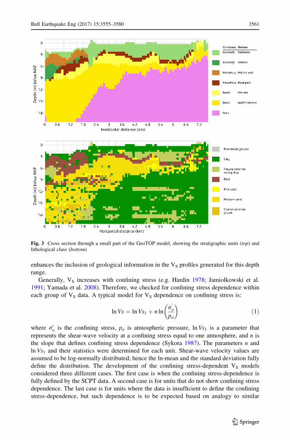
An example of a cross section through the GeoTOP model is presented in Fig. 3,
showing the stratigraphic units in the top panel and the lithological classes in the bottom
panel. From top to bottom there are in this example Holocene Naaldwijk clays, the Holland
and Basal Peat, sands of the Boxtel Formation and clays of the Peelo Formation.
The GeoTOP VS model associates each of the voxels of the GeoTOP model to a VS
value. The various constituents of the Groningen subsoil have different geological histo-
ries, as described above, and consequently have different geomechanical characteristics.
A Holocene clay will have a different VS than a Pleistocene clay that has experienced
loading by ice sheets. Therefore, different VS statistical distributions were derived for each
of the stratigraphic and lithological combinations that are found in the Groningen field. In
the following, the combination of stratigraphy and lithology is referred to as ‘‘unit’’.
A data set of 88 SCPTs in Groningen provided the input for these statistical distribu-
tions. The VS measurements from the SCPTs at each depth were associated with a
stratigraphy, inferred from GeoTOP, and lithological class, inferred from cone resistance
and friction ratio of the accompanying cone penetration test (CPT). The effective isotropic
confining stress, r0
o (i.e., the average of the vertical and two horizontal components of the
effective stress) for each depth is computed using the unit weight of the overlying sedi-
ments and assuming a mean water table of 1 m below the surface. For brevity, the effective
isotropic confining stress is hereafter simply referred to as ‘‘confining stress’’. Next, VS
values from the SCPTs were clustered for each unit and lnVs was plotted versus the natural
logarithm of the confining stress. The clustered VS values were then used to develop
models to assign VS values to each of the GeoTOP voxel-stacks. A voxel-stack is a vertical
sequence of voxels at a particular (x,y)-location in the GeoTOP grid. This approach
3560 Bull Earthquake Eng (2017) 15:3555–3580
123
enhances the inclusion of geological information in the VS profiles generated for this depth
range.
Generally, VS increases with confining stress (e.g. Hardin 1978; Jamiolkowski et al.
1991; Yamada et al. 2008). Therefore, we checked for confining stress dependence within
each group of VS data. A typical model for VS dependence on confining stress is:
lnVs ¼ lnVs1 þ n lnr
0o
pa
� �ð1Þ
where r0o is the confining stress, pa is atmospheric pressure, lnVs1 is a parameter that
represents the shear-wave velocity at a confining stress equal to one atmosphere, and n is
the slope that defines confining stress dependence (Sykora 1987). The parameters n and
lnVs1 and their statistics were determined for each unit. Shear-wave velocity values are
assumed to be log-normally distributed; hence the ln-mean and the standard deviation fully
define the distribution. The development of the confining stress-dependent VS models
considered three different cases. The first case is when the confining stress-dependence is
fully defined by the SCPT data. A second case is for units that do not show confining stress
dependence. The last case is for units where the data is insufficient to define the confining
stress-dependence, but such dependence is to be expected based on analogy to similar
Fig. 3 Cross section through a small part of the GeoTOP model, showing the stratigraphic units (top) andlithological class (bottom)
Bull Earthquake Eng (2017) 15:3555–3580 3561
123

sediments elsewhere in the field. For these units, the parameters of Eq. 1 are based on
existing literature and expert judgment.
Two examples of VS data for typical units with numerous observations are shown in
Fig. 4. The mean VS at a certain confining stress is described by the slope n and the
intercept lnVS1, while the standard deviation depends on the number of observations, mean
ln r00=pa� �
, the sum of squares of ln r00=pa� �
and the total variance of VS (Montgomery et al.
2011). As indicated previously, the VS profiles also need to be randomised (described in
Sect. 4.1), for which the above described mean VS and standard deviation will be used.
There were sufficient observations (a minimum of 20) for 10 units to derive a confining
stress-dependent relation based on SCPT data. The parameters describing the confining
stress dependence defined by the SCPT data are given in Table 1. The values of the slope
n for Groningen clay (including sandy clay and clayey sand) range from 0.18 to 0.43 with
an average of 0.28. This compares well with literature values for clay, which are generally
given as n = 0.25 (Hardin 1978; Jamiolkowski et al. 1991; Yamada et al. 2008). The slope
n depends on the type of sediment (Fig. 4): clays of the Peelo Formation (Pleistocene
glacial deposits) have a stronger confining stress dependence (larger n) than clays of the
Naaldwijk Formation (Holocene tidal deposits) which is generally present at much shal-
lower depths and thus lower confining stresses.
For several units, confining stress dependence is not apparent in the SCPT data, showing
an n close to 0 or even slightly negative. Figure 5 shows VS data for medium sand from the
Boxtel Formation. Since the slope in this case is very close to 0 (0.07), no confining stress
dependence was imposed for this unit. In some other cases, the geological history implies
that confining stress dependence is not expected. For example, the clay from the Drente
Formation formed under varying glacial conditions and the effect of spatially varying
loading is much larger than the confining stress dependence. The distributions of these
constant VS units are defined by the mean and standard deviations of lnVs. These are
summarised in Table 2. A minimum standard deviation of 0.2 is imposed. This lower limit
was used in the past as measurement uncertainty in VS profiles (Coppersmith et al. 2014).
A standard deviation 0.27 is imposed on all peats, based on the observations from the
SCPT data set for Nieuwkoop Holland Peat.
The last class of VS consists of units for which confining stress dependence of VS is to
be expected, but there are not enough data in the SCPT data set to constrain this
Fig. 4 Example of numerous VS observations in the SCPT data set, for clays from the Peelo Formation(left) and Naaldwijk Formation (right). The solid line describes the regression while dotted lines indicate95% confidence intervals
3562 Bull Earthquake Eng (2017) 15:3555–3580
123

relationship. In that case, we estimate n from literature. We use n = 0.25 for clay, for all
lithoclasses within Nieuwkoop Basal Peat and for peats within Pleistocene Formations
following Hardin (1978), Jamiolkowski et al. (1991) and Yamada et al. (2008). For sand,
we use measured coefficients of uniformity Cu from Groningen to estimate n using Menq
(2003). This results in values for n varying between 0.25 and 0.29. In this case, no average
Fig. 5 Example of VS independent of confining stress, n = 0.07 based on the data for medium sand of theBoxtel Formation. For this data set, a slope of n = 0 is chosen. The solid line describes the regression whiledotted lines indicate 95% confidence intervals
Table 1 Look-up table summarising parameters for the confining stress dependent VS (Eq. 1) from SCPTs
Formation Lithological class #Obs.
Slopen
InterceptVS1 (m/s)
Mean
ln r00=pa� � Sum of
squares
ln r00=pa� �
Totalvariance ofln(VS)
Boxtel Sandy clay andclayey sand
43 0.20 217.0 0.10 5.67 0.039
Boxtel Fine sand 260 0.11 247.2 -0.057 64.41 0.054
Naaldwijk Clay 303 0.18 135.6 -1.20 107.49 0.11
Naaldwijk Sandy clay andclayey sand
245 0.28 190.6 -0.98 59.65 0.066
Naaldwijk Fine sand 166 0.36 247.2 -0.78 34.05 0.099
NieuwkoopBasal Peat
Peat 22 0.57 156.0 -0.77 3.70 0.19
Peelo Clay 455 0.33 194.4 0.39 41.89 0.033
Peelo Sandy clay andclayey sand
41 0.43 181.3 0.66 2.59 0.033
Peelo Fine sand 222 0.10 265.1 0.54 16.26 0.022
Peelo Medium and coarsesand, gravel andshells
72 0.24 265.1 0.61 3.04 0.020
During random sampling, a minimum standard deviation of 0.2 is imposed
Bull Earthquake Eng (2017) 15:3555–3580 3563
123
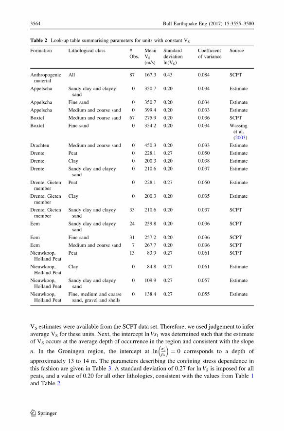
VS estimates were available from the SCPT data set. Therefore, we used judgement to infer
average VS for these units. Next, the intercept lnVs1 was determined such that the estimate
of VS occurs at the average depth of occurrence in the region and consistent with the slope
n. In the Groningen region, the intercept at lnr0opa
� �¼ 0 corresponds to a depth of
approximately 13 to 14 m. The parameters describing the confining stress dependence in
this fashion are given in Table 3. A standard deviation of 0.27 for lnVS is imposed for all
peats, and a value of 0.20 for all other lithologies, consistent with the values from Table 1
and Table 2.
Table 2 Look-up table summarising parameters for units with constant VS
Formation Lithological class #Obs.
MeanVS
(m/s)
Standarddeviationln(VS)
Coefficientof variance
Source
Anthropogenicmaterial
All 87 167.3 0.43 0.084 SCPT
Appelscha Sandy clay and clayeysand
0 350.7 0.20 0.034 Estimate
Appelscha Fine sand 0 350.7 0.20 0.034 Estimate
Appelscha Medium and coarse sand 0 399.4 0.20 0.033 Estimate
Boxtel Medium and coarse sand 67 275.9 0.20 0.036 SCPT
Boxtel Fine sand 0 354.2 0.20 0.034 Wassinget al.(2003)
Drachten Medium and coarse sand 0 450.3 0.20 0.033 Estimate
Drente Peat 0 228.1 0.27 0.050 Estimate
Drente Clay 0 200.3 0.20 0.038 Estimate
Drente Sandy clay and clayeysand
0 210.6 0.20 0.037 Estimate
Drente, Gietenmember
Peat 0 228.1 0.27 0.050 Estimate
Drente, Gietenmember
Clay 0 200.3 0.20 0.035 Estimate
Drente, Gietenmember
Sandy clay and clayeysand
33 210.6 0.20 0.037 SCPT
Eem Sandy clay and clayeysand
24 259.8 0.20 0.036 SCPT
Eem Fine sand 31 257.2 0.20 0.036 SCPT
Eem Medium and coarse sand 7 267.7 0.20 0.036 SCPT
Nieuwkoop,Holland Peat
Peat 13 83.9 0.27 0.061 SCPT
Nieuwkoop,Holland Peat
Clay 0 84.8 0.27 0.061 Estimate
Nieuwkoop,Holland Peat
Sandy clay and clayeysand
0 109.9 0.27 0.057 Estimate
Nieuwkoop,Holland Peat
Fine, medium and coarsesand, gravel and shells
0 138.4 0.27 0.055 Estimate
3564 Bull Earthquake Eng (2017) 15:3555–3580
123

Not all units present in the Groningen region are represented in the SCPT data set. In
those cases, either representative relations from similar units or expert estimates were used
(e.g. Table 3). For example, all members from the Naaldwijk Formation were represented
by the Naaldwijk VS distributions in Table 1 and 3. Additionally, the VS distributions of
Nieuwkoop Holland Peat are assumed to be representative for all Holocene peats.
3.2 MEI VS model
Three-dimensional seismic reflection data was acquired in the 1980s by NAM for the
purpose of imaging and characterisation of the Groningen gas reservoir. This legacy data
set was used to constrain the VS model in the intermediate depth range. Surface waves are
generally regarded as noise in the process of seismically imaging deep reflectors. There-
fore, they are attenuated during acquisition of seismic data and suppressed during pro-
cessing. The surface (and guided) waves, however, propagate along the surface and
therefore contain useful information of the elastic properties of the near-surface. Survey
techniques have been designed that use these types of waves (e.g. Park et al. 1999). Hence,
inversion of these surface waves was used to derive a VS model.
Table 3 Look-up table summarising parameters for the confining stress dependent VS (Eq. 1) fromestimates
Formation Lithological class Slopen
InterceptVS1 (m/s)
Standarddeviationln(VS)
Appelscha, Boxtel, Drachten,Eem, Peelo, Urk-Tynjemember
Peat 0.25 122.7 0.27
Appelscha Clay 0.25 267.7 0.20
Boxtel Clay 0.25 177.7 0.20
Drachten Clay 0.25 146.9 0.20
Drachten Sandy clay and clayey sand 0.25 221.4 0.20
Drente Fine sand 0.25 225.9 0.20
Drente Medium sand 0.25 239.8 0.20
Drente Coarse sand, gravel and shells 0.26 237.5 0.20
Drente, Gieten member Fine sand 0.25 278.7 0.20
Drente, Gieten member Medium sand 0.29 295.9 0.20
Drente, Gieten member Coarse sand, gravel and shells 0.26 295.9 0.20
Eem Clay 0.25 194.4 0.20
Naaldwijk Medium and coarse sand, graveland shells
0.25 308.0 0.20
Nieuwkoop Basal Peat Clay 0.25 141.2 0.27
Nieuwkoop Basal Peat Sandy clay and clayey sand, fine,medium and coarse sand, graveland shells
0.25 170.7 0.27
Urk, Tynje member Clay 0.25 167.3 0.20
Urk, Tynje member Sandy clay and clayey sand 0.25 194.4 0.20
Urk, Tynje member Fine sand and medium sand 0.26 219.2 0.20
Urk, Tynje member Coarse sand, gravel and shells 0.26 265.1 0.20
Bull Earthquake Eng (2017) 15:3555–3580 3565
123
The Modal Elastic Inversion (MEI) method was used for the elastic near-surface model
building. In essence, the MEI method is an approximate elastic Full Waveform Inversion
method, in which the elastic wavefield is approximated by focusing on waves that prop-
agate laterally through the shallow subsurface. These waves include the fundamental mode
of the Rayleigh wave, its higher modes and guided waves. A limited number of hori-
zontally propagating modes, characterized by lateral propagation properties and depth-
dependent amplitude properties, are taken into account to represent the near-surface elastic
wavefield (Ernst, 2013). The objective in the MEI approach is to find a model that min-
imizes the difference between the observed data (Rayleigh waves) and the forward mod-
elled data.
The pre-processing applied to the data prior to Modal Elastic Inversion was restricted to
applying a high-cut filter and data selection of those data traces that contain the Rayleigh
waves. For efficiency, the data set was split in large overlapping rectangular areas, which
were inverted independently. Within one area, all data are inverted simultaneously. The
resulting VS models are merged afterwards. The starting model was a laterally invariant
vertical gradient, which was subsequently updated during the inversion. All lateral vari-
ations in the resulting VS model were introduced by the inversion. Generally, the uncer-
tainty in VS values in the resulting VS model is estimated to be 5–10%.
The vertical resolution of the resulting VS model is limited and the maximum depth
range to which VS in this case can be reliably estimated is approximately 120 m below the
surface. This is due to the seismic data acquisition design and consequently the narrow
frequency band in which the surface waves are unaffected and still present in the data. The
surface seismic data was acquired in 1988 with mostly (buried) dynamite sources and to a
lesser extent with vibroseis sources (in cities) or airgun sources (in lakes and offshore), and
recorded with 10 Hz vertical geophones. The seismic data acquisition was designed for
deep imaging of the Groningen reservoir with a typical orthogonal geometry with line
spacing of 250–500 m and group spacing of 50 m. The receiver group arrays were
designed to suppress and distort Rayleigh waves with wavelengths less than approximately
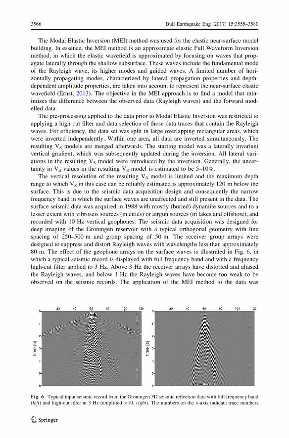
80 m. The effect of the geophone arrays on the surface waves is illustrated in Fig. 6, in
which a typical seismic record is displayed with full frequency band and with a frequency
high-cut filter applied to 3 Hz. Above 3 Hz the receiver arrays have distorted and aliased
the Rayleigh waves, and below 1 Hz the Rayleigh waves have become too weak to be
observed on the seismic records. The application of the MEI method to the data was
Fig. 6 Typical input seismic record from the Groningen 3D seismic reflection data with full frequency band(left) and high-cut filter at 3 Hz (amplified 910, right). The numbers on the x-axis indicate trace numbers
3566 Bull Earthquake Eng (2017) 15:3555–3580
123

therefore restricted to the bandwidth from 1 to 3 Hz, and to those recorded traces on which
the Rayleigh waves were recorded.
The narrow temporal bandwidth results in a narrow range of wavelengths (roughly
between *70 m and *500 m). The penetration depth of the Rayleigh wave depends on
the wavelength: the short wavelengths are sensitive to the shallow subsurface velocities,
whereas the long wavelengths are more sensitive to the deeper velocities. The narrow range
of wavelengths and especially the lack of short wavelengths therefore results in limited
resolving power for the very shallow subsurface velocities. A typical depth resolution
kernel of the fundamental mode of the Rayleigh wave is shown in Fig. 7. The high
frequencies (right side of the plot) are more sensitive to the shallow layers, while the low
frequencies (left side of the plot) are more sensitive to the deeper layers. The maximum
penetration depth is *120 m and there is a limited resolving power of velocities in the
shallow layers of the model (0–20 m).
The convergence of the inversion is verified using the normalized root-mean-square
(RMS) misfit between the model and the data for each seismic shot (Fig. 8). The nor-
malized RMS misfit ranges from 0 (excellent convergence) to 100 (very poor conver-
gence). Generally, Fig. 8 shows that the normalized RMS misfit is good, but there are
several areas with large misfits (denoted by red outlines). These larger misfits are linked to
the source types used during the seismic acquisition. In and around cities or highways
vibroseis sources were used and airguns were used in lakes. Both source types do not
contain the low frequencies required for the inversion. The estimation of the shear-wave
velocity model in these areas might be hampered by these conditions. In other areas, the
seismic records were acquired using buried dynamite sources and show a much better
Fig. 7 Representative depth sensitivity kernel for the fundamental mode of the Rayleigh wave as a functionof depth and frequency. Red indicates low sensitivity, blue indicates high sensitivity
Bull Earthquake Eng (2017) 15:3555–3580 3567
123

RMS. The area in the north is characterized by a high ambient noise level that cannot be
modelled and therefore shows up as a relatively large RMS misfit.
The inversion resulted in a VS model over the area where 3D seismic data was available,
and therefore does not cover the full extent of the area of interest. Horizontally, the VS
model is gridded on the same 100 m 9 100 m grid as the GeoTOP model. Vertically, the
VS model is defined at 10 m depth intervals. An example of a depth slice at 65 m depth is
shown in Fig. 9. The MEI VS model shows distinct zones of relatively high and relatively
low VS values in patterns that resemble geological features, such as buried valleys. These
structures can also be recognized in a cross-section from West to East in the centre of the
field (Fig. 10). The cross-section also shows the vertical smoothness of the model.
3.3 Sonic VS model
For larger depths, VS is derived from the seismic data that was collected to image the
reservoir. One component of the processing of seismic data for imaging is the application
of pre-stack depth migration (Yilmaz 2001), which among others moves dipping reflectors
to their true positions. This procedure requires a velocity model, the so-called Pre-Stack
Depth Migration Velocity model (PSDM velocity model). There are more than 500 wells
in the Groningen field. Data from these wells were available for this project. Sonic logs,
providing VP, were measured in 70 of them. In several wells, VS was measured as well
over a limited depth range. In two wells both VP and VS were measured over the entire
North Sea Supergroup. Sonic logs and well markers for key horizons are used to construct
a depth-calibrated, high-resolution P-wave (VP) model over the entire field. There is
sufficient coverage of sonic logs for depths larger than 200 m, but for shallower depths, the
accuracy of the VP model is reduced.
The PSDM velocity model is used as input VP model for the North Sea Supergroup. Site
response calculations, however, require information in terms of VS instead of VP. Hence,
Fig. 8 Normalized RMS misfit per shot record. Red outlines indicate areas with large misfit due to seismicacquisition source types (vibroseis and airguns)
3568 Bull Earthquake Eng (2017) 15:3555–3580
123

the PSDM VP values are converted to VS using VP/VS relations from the two well logs
where both VP and VS were measured over the entire North Sea Supergroup (Fig. 11). The
measurements of VP and VS start below the depth of the conductor in the well, at
*60–75 m. The ratio between VP and VS shows a linear decrease with depth in the Upper
North Sea Group, while it is more or less constant in the Lower North Sea Group (Fig. 11).
The linear relationship to convert VP into VS for the Upper North Sea Group is given by:
VS ¼VP
4:7819�0:0047 � Zð Þ ð2Þ
where Z is the depth in metres. The corresponding Poisson’s ratio in the Upper North Sea
Group generally varies between 0.45 and 0.47. The constant relation to convert VP into VS
for the Lower North Sea Group is given by:
Fig. 9 Depth slice through theMEI VS model at a depth ofNAP-65 m
Fig. 10 Cross section through the MEI VS model, from west to east at the centre of the field. The verticalscale is exaggerated
Bull Earthquake Eng (2017) 15:3555–3580 3569
123

VS ¼VP
3:2ð3Þ
This corresponds to a Poisson’s ratio of 0.446.
The Sonic VS model was discretised in layers of 25 m thickness and on a grid identical
to the 100 m 9 100 m cells of the GeoTOP model. A cross section of the sonic VS model
through the centre of the field is shown in Fig. 12. The VS inversion which is present in the
Lower North Sea Group at depths of *500 m is caused by the Brussels sand. Locally, this
sand is cemented, leading to high VS.
Fig. 11 VP and VS profiles (left) and the VP/VS ratio (middle) and Poisson’s ratio (right) for two deep wellsin the Groningen field. BRW-5 in blue symbols, ZRP-2 in red symbols
Fig. 12 Cross section through the Sonic VS model, from west to east at the centre of the field. The verticalscale is exaggerated. The base of the Upper North Sea Group is indicated by the black line; the base of theLower North Sea Group by the thin yellow line
3570 Bull Earthquake Eng (2017) 15:3555–3580
123

4 Generation of VS profiles
4.1 Splicing of the final VS models
The three VS models are spliced in order to obtain VS profiles from the surface to the
reference baserock horizon at the base of the North Sea Supergroup for each location in the
field. The top part, from the surface to NAP-50 m, consists of the GeoTOP VS model. The
MEI VS model is appended between NAP-50 m and a maximum of NAP-120 m. The layer
thicknesses in the MEI VS depth range are taken from the geological scenarios of the
geological model below 50 m (Sect. 5). The maximum thickness of layers in this depth
range is 10 m.
The extent of the MEI model is smaller than the extent of the area of interest,
comprising of the Groningen field with a 5 km buffer. For regions outside the MEI
range, the average MEI VS for a depth slice was selected as an estimate of VS. In effect,
this yielded an increasing VS model with depth, but without detailed channel-like
structures.
The transition between the MEI and the sonic VS model is chosen at the depth where the
two VS profiles intersect. This choice avoids velocity inversions at the transition. The layer
thicknesses in the sonic VS range are taken from the geological scenarios of the geological
model below 50 m (Sect. 5) with a maximum thickness of 25 m. The reference rock
horizon is represented by the base of the North Sea Supergroup. At this level, there is an
impedance contrast as VS jumps from *600 m/s (on average) just above this level to
1400 m/s (on average) just below this level. Examples of typical VS profiles constructed
from the three VS models are shown in Fig. 13. In total, approximately 140,000 VS profiles
were generated.
4.2 Randomisation of VS profiles
The spatial variability within each geological zone (Sect. 5) needs to be captured in the site
response analyses. To this end, randomisation was applied in the site response calculations
to the soil composition, input motions (Rodriguez-Marek et al. 2017) and to the VS profiles
in the GeoTOP depth range. Randomisation of soil composition is achieved by assuming
that the collection of GeoTOP voxel-stacks within one geological zone represent the likely
Fig. 13 Examples of VS profiles over the full depth range, with sampled and mean VS in the top 50 m andMEI and Sonic VS below 50 m. The sampling is described in Sect. 4.2. The VS at reference rock horizon(1400 m/s) is out of the horizontal scale
Bull Earthquake Eng (2017) 15:3555–3580 3571
123

successions of units within that zone. The procedure to develop randomised GeoTOP VS
profiles is shown in Figs. 14 and 15. Shear-wave velocity profiles were calculated for each
voxel-stack in the GeoTOP model. For each unit in the voxel-stack (Fig. 14a,b), the
corresponding VS relation is selected from Tables 1, 2, or 3. A sensitivity study indicated
that the 0.5 m layering of GeoTOP created unrealistic site response results. Therefore, the
GeoTOP layers were resampled into layers of 1.0 m, by examining the two voxels within
every metre and selecting one of the voxels at random (Fig. 14c–e). Next, consecutive
voxels of the same unit were merged into one layer up to a maximum thickness of 3.0 m
(Fig. 14f,g). The maximum thickness of 3.0 m was imposed to preserve the confining
stress-dependence of VS.
Within one voxel-stack and one unit of stratigraphy and lithological class we assume
full correlation of VS. This means that all layers of a given unit within one voxel-stack are
based on one sample of VS from the VS distribution of this unit (i.e. from Tables 1, 2, or 3).
Within one voxel-stack and between different units we assume a correlation coefficient qof 0.5. In order to avoid VS profiles that have extremely low or extremely high (and
therefore unrealistic) VS values, the distributions were truncated at two standard devia-
tions. This truncation follows common practice in site response analyses of nuclear
facilities (EPRI 2013). To compensate for the truncation, the VS values are sampled from a
distribution with a standard deviation that is increased by 16%. This value corresponds to
the value that would render a truncated distribution with the desired (target) standard
deviation. A correlated sampling approach was implemented largely following Toro
(1995). The VS distributions were standardized in order to be able to sample in a correlated
way between units having different VS distributions (different average and standard
deviation of lnVS). Truncation was implemented as follows:
Fig. 14 Example of GeoTOP voxel-stack processing. From left to right: (a) original GeoTOP stratigraphicunits; (b) original GeoTOP lithological classes; (c) resampled lithological classes into layers of 1.0 mthickness; (d) resampled stratigraphic units into layers of 1.0 m thickness; (e) random selector used to selectthe upper (grey) or lower (black) voxel; (f) merged lithological classes with a maximum thickness of 3.0 m;(g) merged stratigraphic units with a maximum thickness of 3.0 m. For the clays (green) of the PeeloFormation (purple), the mean depth of the unit is indicated. Far right: bar graph of the sampled shear-wavevelocity profile assigned to the voxels by applying the routine from Fig. 15 to voxel-stacks (f) and (g)
3572 Bull Earthquake Eng (2017) 15:3555–3580
123

1. Draw a random sample ln VSsample
� �from a normal distribution with
l ¼ ln VSmeanð Þ and r� ¼ 1:16rlnVSð4Þ
2. Standardise to a distribution with l = 0 using
ln VSsamplestandardized
� �¼
ln VSsample
� �� l
� �r�
ð5Þ
3. Repeat steps 1 and 2 until
ln VSsamplestandardized
� ���� ���\2:0 ð6Þ
The random sample for each unit is taken at the average depth of occurrence of this unit
in the voxel-stack. For the confining stress-dependent VS relations in Table 1 the standard
deviation is related to the distance to average lnr0opa
� �. In order to avoid sampling in the
confining stress range either outside the range defined by the data, or always at the tails of
the distribution which might results in relatively large standard deviation, the random
sample ln VSsample
� �is taken at the average depth of occurrence of the particular unit,
assuming that this is comparable to the average confining stress.
When moving to the next unit in the voxel-stack, correlated sampling is applied, again
at the average depth of occurrence of the next unit. The correlated sampling is imple-
mented as follows:
1. Draw an auxiliary variable b (needed for standardized and truncated distribution) from
a normal distribution with l = 0 and r = 1.16.
2. Repeat step 1 until |b|\ 2.0.
3. Calculate ln VSsamplestandardized
� �correlated to the previous layer using the correlation
coefficient q and auxiliary variable b using:
ln VSsamplestandardized
� �¼ qln VSpreviouslayerstandardized
� �þ b
ffiffiffiffiffiffiffiffiffiffiffiffiffiffiffiffiffi1� q2ð Þ
pð7Þ
4. Transform ln VSsamplestandardized
� �to ln VSsample
� �using:
ln VSsample
� �¼ lþ r�ln VSsamplestandardized
� �ð8Þ
where l is the mean VS value at that depth.
5. Use ln VSsamplestandardized
� �as ln VSpreviouslayerstandardized
� �in Eq. (7) in the calculation of the next
unit.
Using the above described procedure, the truncated and correlated lnVS is sampled for
each unit at one depth per unit. In order to determine the shear-wave velocities at other
depths of this unit in the voxel stack, the updated intercept lnVs2 is determined using the
slope n of the corresponding distribution and ln VSsample
� �from Eq. 8 for this unit using:
Bull Earthquake Eng (2017) 15:3555–3580 3573
123

lnVs2 ¼ lnVSsample � n lnr0opa
� �ataveragedepth
!ð9Þ
Finally, the lnVS values at all other depths (and thus confining stresses) within this
voxel-stack of this unit are calculated using:
lnVs ¼ lnVs2 þ n lnr0opa
� �ð10Þ
In effect this means that only lnVs1 and not the slope n is randomized in Eq. 1.
Examples of randomized VS profiles are shown in Fig. 16. For reference, the units and
the profiles based on the mean VS relation are included as well. For uniform units, the
confining stress dependent increase in VS is apparent (e.g. in the left panel of Fig. 16). The
correlated sampling ensures that the jumps in VS between units are not unrealistically
large. In some cases, almost the entire profile is sampled in the low side of the mean (e.g.
middle panel of Fig. 16). Because of a correlation coefficient of 0.5, jumps from relatively
high sampled VS to relatively low sampled VS between units is still possible (e.g. right
panel of Fig. 16).
5 Zonation and layering
The geological cross section of Fig. 2 shows that the subsurface in Groningen is hetero-
geneous. As a consequence, the properties that dictate the response to earthquake shaking
will be spatially variable. However, for practical considerations the site response analyses
were conducted for a finite number of zones within the Groningen field (Rodriguez-Marek
et al. 2017). Hence, we defined zones of geologically similar build-up to accommodate for
the heterogeneity of the subsurface. These zones were used as a starting point for the site
response zonation (Rodriguez-Marek et al. 2017).
Several sources of information were available for the definition of the geological zones:
the high resolution 3D geological model GeoTOP (Stafleu et al. 2011; Stafleu and Dubelaar
2016), 19,082 borehole descriptions from the DINO database (www.dinoloket.nl), 5674
cone penetration tests, the Digital Geological Model of the Netherlands (DGM, Gunnink
et al. 2013), the REgional Geohydrological Information System II (REGIS II, Vernes and
van Doorn 2005), the digital terrain model AHN (open data, www.ahn.nl) and paleogeo-
graphic maps (Vos and Knol 2015; Vos et al. 2011).
Because of the difference in resolution and depth range of the various geological
sources, the region of Groningen has been divided into zones of similar geology for two
depth ranges (Kruiver et al. 2015). Between the surface and the maximum depth of
GeoTOP (NAP-50 m), the geological zones are defined based on characteristic succes-
sions. The model consists of a geological zonation map (Fig. 17) and the GeoTOP voxels
with stratigraphic and lithoclass information. This zonation was applied to the site response
results (Rodriguez-Marek et al. 2017), because of the large contribution of the shallowest
deposits to the site response.
cFig. 15 Scheme for sampling of VS. ‘strat-lith’ is short for the combination of stratigraphic unit andlithological class
3574 Bull Earthquake Eng (2017) 15:3555–3580
123

Bull Earthquake Eng (2017) 15:3555–3580 3575
123

In addition to the VS profiles, site response analyses require the assignment of nonlinear
properties to each layer. This assignment is based on the soil type for each layer (e.g. using
Darendeli 2001 or Menq 2003). For the near surface layers, the stratigraphic and lithoclass
information from the GeoTOP model is used to assign soil types to each layer. The deeper
geological structures are different from the shallow structures, hence a different geological
zonation map applies for the depth range between NAP-50 m and the base of the Upper
North Sea Group. The layer and composition information for this depth range which are
needed for assigning appropriate nonlinear properties to each layer is represented by
characteristic scenarios for subsurface successions for each zone, including a probability of
encountering each scenario in that zone. In the site response calculations, the Lower North
Sea Group was considered to behave linearly (Rodriguez-Marek et al. 2017). Therefore,
details on the composition of these layers, beyond its VS value, are not needed. The full
layer profile for each location (X, Y coordinate on the GeoTOP grid) is a combination of
the GeoTOP layers of stratigraphy and lithoclass, appended with one of the deeper sce-
narios while taking into account the probabilities of each scenario on the deeper geological
zones.
6 VS30 map
The time-averaged shear-wave velocity over the upper 30 m of a profile (VS30) is used as
an input to some of the components of the ground motion model for the Groningen region
(Bommer et al. 2017) The GeoTOP VS model enables the determination of a VS30 map.
This map is also relevant for the new building codes in the Netherlands. A VS profile is
calculated between the surface and 30 m depth following the scheme described in Sect. 4,
except that the layers of 0.5 m thickness of GeoTOP have been preserved. The VS30 is then
calculated from the VS profile as the harmonic mean. This procedure was repeated 100
Fig. 16 Three examples of randomized VS profiles (black line) and mean VS profiles (red lines), at thesame locations as Fig. 13. The column at the left of each graph indicates the units in the voxel-stack. Left:example of homogeneous voxel-stack with only 4 units of stratigraphy-lithology. Middle and right:examples of more heterogeneous voxel-stacks
3576 Bull Earthquake Eng (2017) 15:3555–3580
123

times with a different initial random sample for each voxel-stack, which provided 100
estimates of VS30 for each GeoTOP grid cell.
The average and standard deviation of VS30 values for each geological zone were
calculated from all VS30 values within that zone. For the entire field, the average VS30
based on all VS30 realisations is 207 m/s with a standard deviation of 48 m/s. The VS30
maps with zonation are shown in Fig. 18 for mean and standard deviation of VS30. The data
are plotted in coloured bins in these figures; the VS30 data per zone is available in Online
Resource 1. The average and median VS30 are very similar, with a maximum difference of
5 m/s. The maps show a distinct pattern in VS30 that is related to geology. The northern
part of the region contains the thickest layers of soft Holocene deposits, with overall low
VS30 values. Channel structures can be recognised, e.g. in the eastern part. The southern
part consists of Pleistocene deposits which are generally stiffer (but still relatively soft
soil), which is reflected in the higher VS30 values. The Hondsrug (the sand ridge on which
the city of Groningen is situated) stands out as a relatively high VS30 zone in the south
west. Immediately east of the ridge is a channel that is filled with soft Holocene deposits.
This is reflected by the low VS30 zone adjacent to the Hondsrug. The right panel of Fig. 18
shows that the standard deviation of VS30 ranges from 25 to 54 m/s between zones.
Although the VS30 values are relatively low (soft soil), variation of VS30 within zones,
expressed by the standard deviation, can be significant. The degree of variation in VS30
within the zones is not uniform across the entire field. In particular, within-zone variation is
greater in the south where the average VS30 values are higher.
Fig. 17 Geological zonationmap. Similar colours indicatesimilar geological successions inthe shallow depth range
Bull Earthquake Eng (2017) 15:3555–3580 3577
123

7 Discussion and conclusions
In this paper a shear-wave velocity model is presented spanning the depth range from the
surface to about 800 m depth as a starting point for site response analyses in the Groningen
field. The combination of three different VS models (in terms of depth ranges) resulted in a
model that is unique on this scale. Furthermore, a randomisation scheme for the shallow VS
profiles (to 50 m depth) was developed, taking into account the geological characteristics
of the subsurface. This randomisation is required to determine the probabilistic amplifi-
cation factors that feed into the seismic hazard and risk analysis. To facilitate the ran-
domisation of VS, we derived VS relations for each unit of stratigraphy and lithology that is
present in the region. Full correlation of VS is assumed within one unit in a vertical profile.
Between units, however, partial correlation is assumed using a correlation coefficient of
0.5. Additionally, a microzonation model was constructed to account for geological
heterogeneity.
The VS relations for the shallow depth range were based on SCPT data measured in the
region. For some units there was insufficient data to determine a confining stress-dependent
relation. Future fieldwork campaigns will increase the number of SCPTs available for this
analysis. Additionally, there is a large number of CPTs (*5700) available in the region.
This provides the opportunity to design a region specific VS relation based on both SCPTs
and CPTs. When the CPTs are converted to synthetic VS profiles using relations that are
calibrated on the SCPT-CPT data set, more units can be quantified. Rather than using
standard classification methods (e.g. Robertson 1990), the adapted scheme is needed to
accommodate soils such as peats and glacial clays.
Fig. 18 Mean (left) and standard deviation (right) of VS30 for the Groningen region
3578 Bull Earthquake Eng (2017) 15:3555–3580
123

Additionally, the transition between the GeoTOP and MEI VS models is currently
defined at one fixed depth, i.e. the maximum depth of the GeoTOP model. An alternative
choice might be a transition level that varies in depth and is based on the location of
channel structures or other geological features. However, to implement this approach the
exact locations of these features needs to be known and these are currently not known in
sufficient detail. Future subsurface models by TNO—Geological Survey of the Netherlands
may include the required level of detail. In the current model, scenarios of stratigraphy
were used below NAP-50 m to accommodate the uncertainty in locations of key geological
features.
The model building presented in this paper represents a unique exercise in which a
comprehensive set of geological, geotechnical, and geophysical data was used to build an
extensive 3D VS model for site response analyses. The construction of this deep and
detailed VS model has enabled the incorporation of fully probabilistic, nonlinear site
amplification functions into the estimation of surface ground motions (Rodriguez-Marek
et al. 2017). In essence, an approach to including local site effects in seismic hazard
analyses usually applied in site-specific studies for critical facilities can thus be applied to
hazard and risk assessments for an entire region (Bommer et al. 2017).
Acknowledgements The geological zonation model was constructed by a large team of geologists fromDeltares and TNO—Geological Survey of the Netherlands: Ane Wiersma, Pieter Doornenbal, TommerVermaas, Renee de Bruijn, Marc Hijma, Freek Busschers, Marcel Bakker, Ronald Harting, Roula Dambrink,Willem Dabekaussen, Wim Dubelaar, Eppie de Heer, Jan Peeters. Veronique Marges provided numerousmaps and Wim Dubelaar commented on the geological setting. We are very grateful to several individualswho have provided critical review and feedback at different stages of the project. We wish to express ourgratitude to Ben Edwards, Rien Herber, Tijn Berends, Joep Storms, Adriaan Janszen, Karel Maron, ClemensVisser, Bernard Dost and Dirk Kraaijpoel for their comments on the geological zonation model. This paperbenefitted from the comments of an anonymous reviewer.
Open Access This article is distributed under the terms of the Creative Commons Attribution 4.0 Inter-national License (http://creativecommons.org/licenses/by/4.0/), which permits unrestricted use, distribution,and reproduction in any medium, provided you give appropriate credit to the original author(s) and thesource, provide a link to the Creative Commons license, and indicate if changes were made.
References
Bazzurro P, Cornell CA (2004a) Ground-motion amplification in nonlinear soil sites with uncertain prop-erties. Bull Seismol Soc Am 94:2090–2109
Bazzurro P, Cornell CA (2004b) Nonlinear soil-site effects in probabilistic seismic hazard analysis. BullSeismol Soc Am 94(6):2110–2123
Bommer JJ, Stafford PJ, Edwards B, Dost B, van Dedem E, Rodriguez-Marek A, Kruiver PP, van Elk J,Doornhof D (2017) Framework for a ground-motion model for induced seismic hazard and riskanalysis in the Groningen gas field, the Netherlands. Earthq Spectr 33(2). doi:10.1193/082916EQS138M
Bourne SJ, Oates SJ, Bommer JJ, Dost B, van Elk J, Doornhof D (2015) A Monte Carlo method forprobabilistic hazard assessment of induced seismicity due to conventional natural gas production. BullSeismol Soc Am 105:1721–1738
Chiles J-P, Delfiner P (2012) Geostatistics—modeling spatial uncertainty. Wiley, Hoboken, p 699Coppersmith KJ, Bommer JJ, Hanson KL, Unruh J, Coppersmith RT, Wolf L, Youngs R, Rodriguez-Marek
A, Al Atik L, Toro G (2014) Hanford sitewide probabilistic seismic hazard analysis. PNNL-23361Pacific Northwest National Laboratory, Richland Washington http://www.hanford.gov/page.cfm/OfficialDocuments/HSPSHA
Darendeli M (2001) Development of a new family of normalized modulus reduction and material dampingcurves. Dissertation, Department of Civil Engineering, University of Texas, Austin, TX
Bull Earthquake Eng (2017) 15:3555–3580 3579
123

de Mulder EFJ, Geluk MC, Ritsema I, Westerhoff WE, Wong TE (2003) De ondergrond van Nederland.Wolters-Noordhoff
Electrical Power Research Instititue, EPRI (2013) Seismic evaluation guidance. Screening, prioritizationand implementation details (SPID) for the Resolution of Fukushima Near-Term Task Force Recom-mendation 2.1: Seismic. Report no. 1025281. February
Ernst F (2013) Modal elastic inversion. In: 75th EAGE Conference & exhibition incorporating SPEEUROPEC 2013, London, 2013. doi:10.3997/2214-4609.20130001
Goovaerts P (1997) Geostatistics for natural resources evaluation. Oxford University Press, New York,p 483
Gueguen P, Cornou C, Garambois S, Banton J (2007) On the limitation of the H/V spectral ratio usingseismic noise as an exploration tool: application to the Grenoble valley (France), a small apex ratiobasin. Pure Appl Geophys 164(1):115–134
Gunnink JL, Maljers D, Van Gessel SF, Menkovic A, Hummelman HJ (2013) Digital Geological Model(DGM): a 3D raster model of the subsurface of the Netherlands. Neth J Geosci 92:33–46
Hardin BO (1978) The nature of stress–strain behavior for soils. In: ASCE Geotechnical EngineeringDivision Specialty Conference, Pasadena, California, June 19–21, 1978
Havenith HB, Fah D, Polom U, Roulle A (2007) S-wave velocity measurements applied to the seismicmicrozonation of Basel, Upper Rhine Graben. Geophys J Int 170(1):346–358
Jamiolkowski M, Leroueil S, Lo Presti D (1991) Theme lecture: design parameters from theory to practice.In: Proceedings, Geo-Coast, vol 2. Pp 877–917
Kruiver PP, de Lange G, Wiersma A, Meijers P, Korff M, Peeters J, Stafleu J, Harting R, Dambrink R,Busschers F, Gunnink JL (2015) Geological schematisation of the shallow subsurface of Groningen—for site response to earthquakes for the Groningen gas field. Deltares report no. 1209862-005-GEO-0004-v5-r. http://kennisonline.deltares.nl/product/30895
Menq F (2003) Dynamic properties of sandy and gravelly soils. Dissertation, University of TexasMontgomery DC, Runger GC, Hubele NF (2011) Engineering statistics. WileyPark CB, Miller RD, Xia J (1999) Multichannel analysis of surface waves (MASW). Geophysics
64:800–808Pitilakis K, Raptakis D, Lontzetidis K, Tika-Vassilikou T, Jongmans D (1999) Geotechnical and geo-
physical description of EURO-SEISTEST, using field, laboratory tests and moderate strong motionrecordings. J Earthq Eng 3(3):381–409. doi:10.1080/13632469909350352
Robertson PK (1990) Soil classification using the cone penetration test. Can Geotech J 27(1):151–158Rodriguez-Marek A, Kruiver PP, Meijers P, Bommer JJ, Dost B, van Elk J, Doornhof D (2017) A regional
site response model for the Groningen gas field. Re-submitted to Bulletin of the Seismological Societyof America following revision
Soares A (1992) Geostatistical estimation of multi-phase structure. Math Geol 24(2):149–160Stafleu J, Dubelaar CW (2016) Product specification subsurface model GeoTOP, version 1.3. TNO report
R10133, 53 pp. https://www.dinoloket.nl/en/subsurface-modelsStafleu J, Maljers D, Gunnink JL, Menkovic A, Busschers FS (2011) 3D modelling of the shallow sub-
surface of Zeeland, the Netherlands. Neth J Geosci 90:293–310Sykora DW (1987) Examination of existing shear wave velocity and shear modulus correlations in soils.
Corps of Engineers, VicksburgToro GR (1995) Probabilistic models of site velocity profiles for generic and site-specific ground-motion
amplification studies. Upton, New YorkVernes RW, van Doorn THM (2005) Van Gidslaag naar Hydrogeologische Eenheid—Toelichting op de
totstandkoming van de dataset REGIS II. TNO report report 05-038-B, 105 ppVos PC (2015) Origin of the Dutch coastal landscape. Long-term landscape evolution of the Netherlands
during the Holocene, described and visualized in national, regional and local palaeogeographical mapseries. Dissertation, Utrecht University
Vos PC, Knol E (2015) Holocene landscape reconstruction of the Wadden Sea area between Marsdiep andWeser. Neth J Geosci 94:157–183
Vos PC, Bazelmans J, Weerts HJT, van der Meulen MJ (2011) Atlas van Nederland in het Holoceen:landschap en bewoning vanaf de laatste ijstijd tot nu. Bert Bakker, Amsterdam
Wassing BBT, Maljers D, Westerhoff RS, Bosch JHA, Weerts HJT (2003) Seismisch hazard van geındu-ceerde aardbevingen, Rapportage fase 1. TNO Geological Survey of the Netherlands Report numberNITG-03-185-C-def (in Dutch)
Yamada S, Hyodo M, Orense RP, Dinesh S (2008) Initial shear modulus of remolded sand-clay mixtures.J Geotech Geoenviron Eng 134:960–971
Yilmaz O (2001) Seismic data analysis. Investigations in Geophysics. Society of Exploration Geophysicists,Tulsa. doi:10.1190/1.9781560801580
3580 Bull Earthquake Eng (2017) 15:3555–3580
123
Top Related