


![1[1].AirPollution Introduction R1](https://static.fdocuments.us/doc/165x107/577d36ef1a28ab3a6b945cdc/11airpollution-introduction-r1.jpg)


Languages
Pages
Legal


GEOS 3310 Lecture Notes: AirPollution
Dr. T. Brikowski
Spring 2011
file:airPollution.tex,v (1.20, January 11, 2011), printed April 22, 2011

Introduction
• see EPA Air Quality Trends (2010) for
good summary
• and AirNow for nationwide current AQI
and much background information
1

Introduction
• air pollution is the most widespread human impact on the
planet
• many trends are encouraging, for instance for the U.S. as awhole air quality is improving [Fig. 17.10, Keller, 2000]
• some are discouraging, e.g. the number of unhealthful days
is increasingly a result of ozone pollution (Fig. 3)
• Texas (especially Houston, Figs. 4–5) stands out as one of
the worst areas of increasing air pollution
– Dallas Metroplex trends are mixed, but generally show
increasing ozone as the number of vehicle miles/day
increases (compare 2005 to 2004 )2
– the Metroplex is chronically out of compliance with
EPA regulations, and new lower standards have brought
increased regulatory pressure
– enforcement may increase with new regional EPA
administrator
3

Air Quality Trends, U.S.
Figure 1: Air quality index trends in the U.S. for six principal pollutants,
1990-2007. From USEPA .
4

AQI
Figure 2: Air Quality Index (AQI) scale. An AQI for each major pollutant
is computed using various EPA formulas . The highest AQI among all the
pollutants is reported for that day.
5

Ozone Impact on AQI
Figure 3: Ozone contribution to increase in air quality index. Increasing
air pollution is chiefly a result of increased ozone pollution, which in turn is
chiefly a result of automobile exhaust. See USEPA air quality trends .
6

Houston-LA Ozone Trends
Figure 4: Trend in number of high ozone days for Houston and Los
Angeles. Both cities experienced similar growth rates during this period, LA
population is approximately 3.7 million, Houston 2 million. After GHASP
webpage.7

US City Smog Rankings
Figure 5: Ranking of major US cities by number of standard-exceeded
days. After GHASP webpage.
8

Ozone Kills
• a 2004 study [Bell et al., 2004] shows Dallas as the U.S. city
with the 8th largest link between deaths and ozone increase
• a 10ppb decrease in average ozone would reduce daily death
rates by 1%
• annual expected deaths from all causes in Dallas County are
40.6/100,000 population, or about 1,000/year (2,500/yr in
Metroplex)
9

Los Angeles Smog
Figure 6: Pasadena looking north at the San Gabriel Mountains with and
without smog. Left image typical of mid-summer days, right image typical
of mid-winter. After California Smog Check webpage.
10
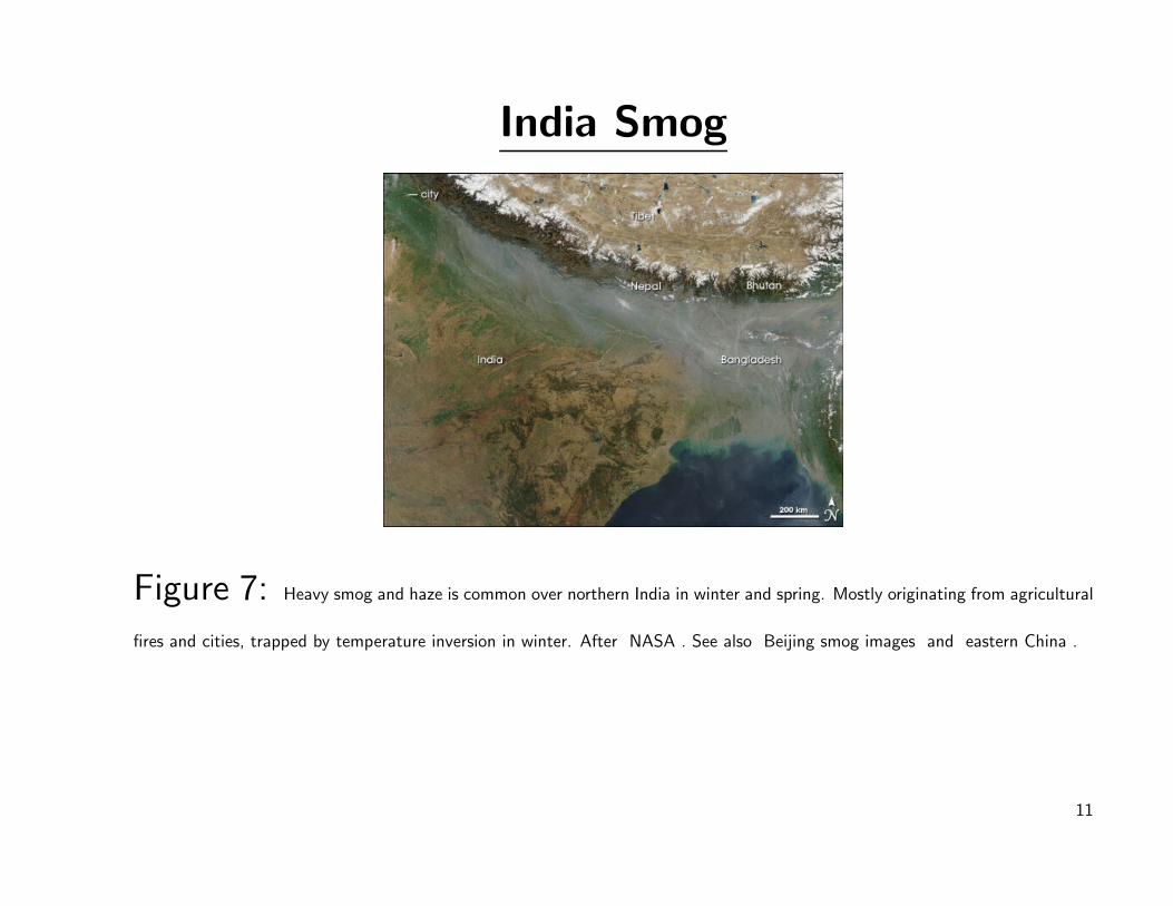
India Smog
Figure 7: Heavy smog and haze is common over northern India in winter and spring. Mostly originating from agricultural
fires and cities, trapped by temperature inversion in winter. After NASA . See also Beijing smog images and eastern China .
11

The Nature of Pollution
12
Pollution Events
Awareness of the seriousness of urban pollution has been
raised by a number of extreme events:
• a number of cases like Ducktown Tennessee have
demonstrated the magnitude of air pollution’s effects
• 1930 Meuse Valley, Belgium. A week long inversion led to
dense smog and 60 deaths
• 1948 Donora, Pennsylvania. Smog related to coal burning
for steel production and household heating led to 20 deaths,
14,000 illnesses
• 1952 London smog crisis: up to 12,000 dead, extremely13

dense smog related to coal burning for heat and industry
[Fig. 18.1, Keller, 2008]. See also NPR story and photos
• Principal smog effects:
– Soils and water: toxic elements added, nutrients leached
– Vegetation: damage to leaves, etc., increased susceptibility
to disease
– Animals: impairment of respiratory system, damage to
body
– Human health: poisoning, respiratory ailments (especially
asthma)
– Human artifacts: discoloration, erosion, etc. (e.g. ozone
causes rubber to fail rapidly)
– Aesthetics: ruined views, especially of natural areas like
the Grand Canyon14

Source Categories
• Stationary: fixed location, includes fugitive, point and area
sources
• Point: emits from a discrete (controllable) site
• Fugitive: open areas that generate particulates
• Area: emit from distributed or multiple sources within a
well-defined area
• Mobile: moving source, e.g. vehicles
15

Pollutants Categories
• gaseous
• particulate: small solid particles, e.g. PM-10 are particles
less than 10 microns
• primary pollutants are emitted directly into the air
• secondary pollutants are formed when primary pollutants
react or combine (e.g. ozone)
16

Major Pollutants
• sulfur dioxide
– colorless and odorless, associated with gray smog
– primarily from coal-fired power plants
– major component of acid rain
– major impact is corrosion of paint and metals, crop
damage, and plant damage in general [Fig. 18.9, Keller,
2008]
• Nitrogen Oxides
– many forms, most prominently NO2, light brown gas
– toxic and quite corrosive
– its major impact is in the formation of photochemicalsmog, secondary contribution is as acid rain
17

– newly recognized as making significant contribution to
ozone layer depletion
– almost all NOx is anthropogenic, mostly automobiles and
power plants
• CO, carbon monoxide
– main impact is to interrupt blood oxygen uptake, causing
asphyxia
– sometimes so high in Los Angeles outdoor air that
household detectors sound alter
– mostly natural sources, but in city it is concentrated
automobile emissions
• Ozone18

– a photochemical oxidant produced by sunlight acting on
several primary pollutants
– main impact is plant and lung tissue damage, breakdown
of rubber, paint, etc.
– main source is automobiles (which release the precursors
of ozone)
• VOC’s, volatile organic compounds
– an important constituent in forming photochemical smog
– globally only 5% of emissions are anthropogenic, but half
the emissions in the U.S. are anthropogenic, primarily
automobiles
– other large sources are 2-stroke engines (e.g. leaf blowers),
charcoal lighter fluid, etc.19

• PM-10: particulate matter
– main sources are industrial processes, power plant effluent
and disturbed ground (dust)
– acts as a lung irritant, and causes significant lung damage
– important particulates are sulfates and nitrates, which are
secondary pollutants
– globally most particulates are natural, but in cities
anthropogenic particulates may dominate
– reduction in particulate pollution shown to increase life
expectancy in the U.S. by 5% (see interactive graphic )
20

Urban Air Pollution
21

Inversions
• meteorological conditions can act to trap pollutants, making
them deadly
• atmospheric inversions occur when cold air is trapped in an
enclosed area (e.g. valley) by overlying warm air [Fig. 18.6,
Keller, 2008]
• these are especially a problem in the Western U.S., where
topography favors trapping of air [Fig. 18.7, Keller, 2008].
See also Mexico City image , although that city has cleaned
up its air remarkably
• the chimney effect allows pollutants to move past
topographic barriers if emissions are high (concentrating22

pollutants) and horizontal winds are sufficient to perturb the
inversion layer [Fig. 18.8, Keller, 2008]
• the heat island effect traps pollutants in cities by limiting
horizontal air circulation when air heated over pavement
moves vertically upward in a convective pattern [Fig. 17.6,
Keller, 2000]
• see also satellite observations
23

Smog Production
• sulfurous smog:
– produced when SO2 and particulates combine with
moisture
– a thick gray fog is produced
– mostly occurs in areas of extensive coal burning (e.g. steel
mill towns) [Fig. 18.9, Keller, 2008]
• photochemical smog
– produced by combination of NOx and hydrocarbon primary
pollutants in the presence of sunlight [Fig. 18.10a, Keller,
2008]
– note this is a complex reaction that is incompletely
understood24

– formation of this smog is directly related to automobile use
– as morning traffic builds up NO and Hydrocarbon
concentrations increase [Fig. 18.10b, Keller, 2008]
– ozone is produced by photodissociation of NO2
– simultaneously hydrocarbons react with NO yielding more
NO2
– by midday peaks in ozone and NO2 (brown haze) are seen
25

Control of Air Pollution
• problems vary by region. In the west and Texas
most problems relate to ozone/photochemical smog (i.e.
automobile-caused). In the upper mid-West it is SO2 and
particulates from coal-fired power plants
• pollution control methods vary by pollutant
• particulates
– mostly from point sources (readily identified)
– controlled mostly by gravity settling, a relatively cheap
process [Fig. 18.14a-b, Keller, 2008]
• automobile pollution is controlled primarily by the catalyticconverter, which transforms CO and hydrocarbons into CO2
26
and water. Separate devices for minimizing NOx emissions
have recently been required as well.
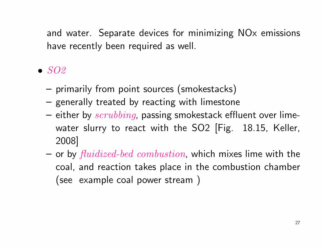
• SO2
– primarily from point sources (smokestacks)
– generally treated by reacting with limestone
– either by scrubbing, passing smokestack effluent over lime-
water slurry to react with the SO2 [Fig. 18.15, Keller,
2008]
– or by fluidized-bed combustion, which mixes lime with the
coal, and reaction takes place in the combustion chamber
(see example coal power stream )
27

Air Quality Legislation
• much of the improvement in U.S. air quality is attributable
to legislation
• the 1970 Clean Air Act set primary standards to protect
people’s health, and less-stringent secondary standards for
plants and other materials
• 1990 amendments to this established cap and tradeapproaches to SO2, where emission reductions at one site
can be used to offset increases at another. Essentially the
right to pollute can be sold on the open market
• EPA’s Clean Air Mercury rule applies “cap and trade”28

to mercury, perhaps unwise for elements subject to
biomagnification
• cost of controls can be optimized, or in some critical cases
mandated (e.g. EPA and lead recycling) [Fig. 18.16, Keller,
2008]
29

Other Resources
30

Useful LinksThis is intended to be an ever-evolving list of useful links on
the general topic of this note set.
• ozone forecast now available for Texas (most states have
similar sites)
• animation of global CO “pollution” transport. Forest and
grassland fires in Africa & South America, industrial pollution
in Southeast Asia.
• animation of global ozone showing seasonal variation by
hemisphere, and hole in Antarctica
• regional high ozone in central Texas contributes to lack of
compliance31

• ozone breaks down flower scent, possibly explaining decline
of bees in some areas
• atmospheric chemistry of photochemical smog
• ozone formation animation
• natural H2S emissions from anaerobic bacteria after “Dead
Zone” phenomena. Same thing eventually led to Permo-
Triassic mass extinction
• more whale sunburns , related to ozone hole?
32

Bibliography
33

Michelle L. Bell, Aidan McDermott, Scott L. Zeger, Jonathan M. Samet, and Francesca Dominici.Ozone and Short-term Mortality in 95 US Urban Communities, 1987-2000. JAMA, 292(19), 17 November 2004.
E. A. Keller. Environmental Geology. Prentice Hall, Upper Saddle River, NJ, 8th edition, 2000.ISBN 0-13-022466-9.
E. A. Keller. Introduction to Environmental Geology. Prentice Hall, 4th edition, 2008.ISBN 9780132251501. URL http://www.pearsonhighered.com/educator/academic/product/0,3110,0132251507,00.html.
34
Top Related