


Languages
Pages
Legal

Air Pollution as a Cause of Violent Crime:Evidence from Los Angeles and Chicago ∗
Evan Herrnstadt†Anthony Heyes
Erich MuehleggerSoodeh Saberian
Job Market Paper
December 2016Current version can be found here
Abstract
Exposure to air pollution has adverse impacts on human health, workplace productivity,and educational and cognitive performance. However, empirical evidence linking pollutionexposure to high-stakes decisionmaking is limited. Motivated by research from medicine andpsychology linking pollution to aggression, we provide the first evidence of a causal link be-tween short-run variation in ambient pollution and the commission of violent crime. Usingthe location of crimes and wind direction as a source of pollution variation, we find that airpollution increases violent crime in both Chicago (by 2.2%) and the Los Angeles metro area (by6.1%). Consistent with the literature on aggression and ambient pollution, we find no effecton property crime. The results are robust to a wide variety of specifications and falsificationtests. Back of the envelope calculations indicate that the cost of pollution-induced crime iscomparable in magnitude to other outcomes studied in the literature and should be includedin benefit-cost analysis of pollution abatement policies. Overall, the results suggest that pollu-tion may reduce welfare and affect behavior and decisionmaking through an even wider set ofchannels than previously understood.
∗We thank William Greene, Pierre Brochu, Sophie Bernard, Doug Miller, Solomon Hsiang, Aureo de Paula, MichaelGreenstone, Rema Hanna, Paulina Oliva and seminar participants at University of Montreal, McGill University, Re-sources for the Future, UC-Berkeley, UC-Irvine, UC-Davis, the June 2016 Summer AERE meetings in Breckenridge andthe March 2016 Congress of the Royal Economic Society in Brighton for valuable comments. Heyes acknowledgesfunding from the Canada Research Chair programme. Herrnstadt acknowledges funding from Resources for the Fu-ture. Heyes is also part-time Professor of Economics at the University of Sussex. Errors are ours.†Herrnstadt: Center for the Environment, Harvard University, [email protected]. Heyes: Department of
Economics, University of Ottawa. Muehlegger: Department of Economics, University of California-Davis and NBER;Saberian: Department of Economics, University of Ottawa.
1
1 Introduction
Air pollution can have a detrimental impact on human well-being in a variety of ways. A large
body of research has quantified a range of adverse effects on adult and infant health.1 More
recent work points to a much wider set of negative impacts, linking variation in air quality to
reduced workplace productivity, diminished labor market participation2, compromised cogni-
tion and test scores3 and costly avoidance behavior4. In this paper, we show that the influence
of air pollution on human behavior and social outcomes is even wider than previously estab-
lished. Specifically, we provide robust quasi-experimental evidence of a positive causal link
from ambient air pollution to same-day violent criminal activity in Chicago and Los Angeles.
Our identification strategy exploits variation in pollution driven by day-by-day changes in
the wind direction. Wind transports air pollution through urban and suburban environments.
Depending on the direction from which the wind is blowing, neighborhoods experience differ-
ential changes in air quality conditions. Using detailed information about where crime occurs
and flexibly controlling for local weather and economic conditions, we compare relative levels
of criminal activity in neighborhoods on days where one part of the city experiences a wind-
driven surge in pollution to days where other parts of the city experience a surge in pollution.
In effect, we are using within-metro, within-day variation in pollution exposure driven by dif-
ferences in wind direction.
We examine the relationship between crime and pollution in the second and third most pop-
ulous cities in the United States: Los Angeles and Chicago. In Los Angeles, ocean winds blow-
ing on-shore push pollution from downtown Los Angeles to the northeast, into the foothills of
the San Gabriel mountains. The San Gabriel mountains trap the pollution, elevating ambient
pollution levels in communities in the foothills (such as Pasadena, Burbank and Glendora),
except where there is a break between mountain ranges (such as at Santa Clarita). To establish
a causal relationship between pollution and crime, we compare criminal activity in areas like
Pasadena relative to activity in areas elsewhere in the Los Angeles metro area on days with
and without winds blowing in from sea. Consistent with the literature from other fields on air
pollution and aggressive behavior, we find violent crime increases in locations adversely im-
pacted by wind-driven pollution. On treated days (where treatment means a west-wind day in
an area where west-wind is associated with dirtier air) violent crime is 6.1 percent higher than
1These include Schlenker and Walker (2016), Currie and Walker (2011), Beatty and Shimshack (2014).2Hanna and Oliva (2015), Zivin and Neidell (2012)3Lavy et al. (2014)4Ito and Zhang (2016), Moretti and Neidell (2011), Zivin and Neidell (2009)
2
on untreated days, relative to control neighborhoods.
We apply a related but distinct identification strategy in Chicago: we focus our attention
on major interstates that transect the city of Chicago (I-90, I-94, I-290, I-55 and I-57) and gener-
ate substantial local air pollution. Exploiting the city block location of the two million crimes
reported to the Chicago police from 2001 - 2012, we estimate the causal effect of pollution on
criminal activity by comparing crime on opposite sides of major interstates on days when the
wind blows orthogonally to the direction of the interstate. As an example, I-290 runs due west
from the Chicago city center to the suburbs of Oak Park and Berwyn. On days when the wind
blows from the south, the pollution from the interstate impacts on the north side of the in-
terstate, whereas when the wind blows from the north, the pollution impacts neighborhoods
south of the road. By comparing relative criminal activity on opposite sides of I-290 on days
when the wind is blowing to the south versus the north, we can control for the main threat to
panel identification: omitted variables plausibly correlated with both pollution and criminal
activity, such as economic activity. The side of the interstate from which the wind blows acts as
a control that captures variation in day-to-day crime, local weather conditions and unobserv-
ables, such as neighborhood economic activity. On days when the wind blows orthogonally to
the interstate, we find that violent crime increases by 2.2 percent on the downwind side. These
effects are unique to violent crimes – consistent with expectations, we find no effect of pollution
on the commission of property crime. When we break the result down by the specific type of
crime, we find evidence that pollution causes assaults to escalate into physical battery, perhaps
suggesting that loss of self-control is an important mechanism. No subcategory of property
crime is affected.
As further evidence that we are identifying a causal effect of air pollution, the effect sizes
in both cities attenuate as wind speeds increase; this finding is consistent with wind-driven
pollution dispersion. In Chicago, the effect also attenuates when we broaden the range of
wind directions considered orthogonal to an interstate. As a placebo test, we consider placebo
“roads” parallel to I-290 as a form of falsification test and find that the downwind estimate is
maximized precisely at the latitude at which I-290 transects Chicago.
Although we use wind direction as our source of quasi-experimental variation in both Los
Angeles and Chicago, the strategies for causal identification differ, as do the potential threats to
identification. Taken together, the robust and consistent results across cities and identification
strategies are more persuasive than either individual analysis alone. In Los Angeles, we use
unique local topography to estimate the effect from within-day variation in pollution in crime
3
across the entire metro area; in Chicago, we focus at a much more local level by isolating sides
of major highways. In the case of Los Angeles, the pollution is generated by many sources
(both mobile and stationary) rather than very localized exposure to pollution from a nearby
interstate. In contrast, in Chicago, for each treated side of the interstate, we can use the op-
posite side of the same interstate as a control, for which economic activity, weather and other
correlates of criminal activity are virtually identical and unlikely to be spuriously correlated
with seasonal fluctuations in wind direction.
Our paper has clear implications for policy. Crime is a major social concern and the ef-
fect sizes that we uncover translate into substantial external costs. Properly accounting for the
impacts of pollution on criminal behavior would increase our estimates of marginal damages,
thus increasing the optimal stringency of externality-correcting regulations or Pigouvian pol-
lution taxes. At a broader level the analysis pushes further at the nexus between the economy,
society, and natural environment, widening the set of economic and social outcomes that can
plausibly be linked to prevailing environmental conditions. A clean city could be not just a
healthy and economically productive city, but also a less violent one.
The rest of the paper proceeds as follows. In Section 2 we summarize the existing literature
in biology, medicine and psychology linking air pollution to aggressive behavior. Although
ours is the first paper to document a causal effect of air pollution on violent crime, previous
research highlights several possible channels that – individually or in combination – might un-
derpin the effects that we find. Section 3 summarizes our data sources. In this section, we
also present some cross-sectional/panel regression results that suggest a positive association
between ambient air pollution levels and same-day violent crime. Acknowledging the prob-
lems with drawing conclusions about causality from this analysis we turn to the central quasi-
experimental elements of the paper in Sections 4 (Overview), 5 (Los Angeles) and 6 (Chicago).
Section 7 brings the results together and develops some policy implications.
2 Pollution and Violence
This paper is the first, to our knowledge, to document the causal relationship between air
pollution and the commission of violent crime.5 We remain agnostic on the mechanism (or
5A distinct literature links long-term exposure to lead with violent crime. Using annual state level crime data forColumbia from 1985 to 2002, Reyes (2007) estimates the elasticity of violent crime with respect to childhood lead ex-posure to be about 0.8. Stretesky and Lynch (2004) exploit spatial variation in lead exposure across 2,772 US countiesto establish a similar link, with the greatest effect in the poorest areas. Nevin (2007) finds a strong, robust correlationbetween violent crime and preschool lead exposure in a panel of high-income countries.
4
mechanisms) underpinning the results that we identify. However, it is useful at this stage
to note that there exist substantial literatures in medicine, biology and psychology that link
pollution exposure to aggression and highlight potential pathways by which ambient pollution
might generate violent behavior.
The first, and perhaps most straightforward pathway, is that pollution might trigger a psy-
chological response as a result of physical discomfort associated with air pollution exposure.6
A long literature in psychology summarized by (Anderson and Bushman, 2002) documents a
link between physical discomfort and aggressive behavior. Most relevant to our work, Rotton
(1983) and Rotton et al. (1978) found laboratory exposure to malodorous reduced subject cog-
nitive performance, tolerance for frustration, and the subjects’ ratings of other people and the
physical environment.7
A second documented pathway linking pollution and aggression is that air pollution may
directly affect brain chemistry. Serotonin (5-Hydroxytrlptamine or 5-HT) is a primary neuro-
transmitter, responsible for the flow of information in the brain and nervous system. Krueger
et al. (1963) was the first study to identify short-term variations in air quality as an important
cause of fluctuations in serotonin in the bloodstream. In more recent work, Paz and Huitron-
Resendiz (1996), Gonzalez-Guevara et al. (2014) and Murphy et al. (2013) provide experimental
evidence linking short-term ozone exposure to decreased serotonin in the brains of animals.8
Serotonin is an inhibitor, low levels of which are associated with increased aggression in
humans and animals, in both observational and experimental settings (Coccaro et al., 2011).
Decreased serotonin is associated with an increased tendency to fight amongst rhesus mon-
keys (Faustman et al., 1993) and increased impulsive aggression in children (Frankle et al.,
2005). In a recent study that involved manipulating the serotonin levels of human subjects
within a social experimental setting, Crockett et al. (2013) found that “serotonin-depleted par-
ticipants were more likely to punish those who treated them unfairly, and were slower to accept
fair exchanges”. In their summary of the human subject literature, Siegel and Crockett (2013)
6Ambient air pollution exposure is known to manifest in physical discomfort. For instance, Nattero and Enrico(1996) followed 32 subjects over the span of nine months and found that high concentrations of ambient CO and NOxwere both significantly correlated with incidence of headache. In addition, ambient pollution causes irritation of theeyes and respiratory system.
7Similar results have been demonstrated when subjects are exposed to uncomfortable temperatures (Baron and Bell,1976), noise (Donnerstein and Wilson, 1976) and other physical discomforts. The link between temperature and crimeis also well-documented (Ranson, 2014).
8Other neurotransmitters have also been implicated, but the mechanisms are not as well-understood. For exampleKinawy (2009) find that rats exposed to the fumes of unleaded or leaded gasoline are more aggressive (adopted moreaggressive postures, attacked others sooner and more frequently) than a control group exposed to clean air. Subsequentinspection of the brains showed variation in the levels not just of serotonin but other monoamine neurotransmitterssuch as dopamine and norepinephrine.
5

note that “...a meta-analysis encompassing 175 independent samples and over 6,500 total par-
ticipants reveals a reliable inverse relationship between serotonin and aggression”. Given that
criminal assault requires both an attacker and a victim, it may also be significant that serotonin
levels are positively correlated with harm-avoidance behavior in humans (Hansenne et al.,
1999); in other words, a serotonin-depleted individual is less likely to seek to avoid or flee from
an aggressor.
Third, exposure to common air pollutants also leads to oxidative stress and the inflam-
mation of nerve tissues in the body and the brain (neuro-inflammation); “(c)onsistent with
findings from human populations, animal studies in dogs, mice and rats show that short-run
exposure to air pollution leads to an immediate increase in neuro-inflammation” (Levesque
et al., 2011; Van Berlo et al., 2010). Neuro-inflammation is linked to aggressive behavior in
animals in experimental settings – Rammal et al. (2008) finds that oxidative stress and inflam-
mation reduces the time to attack and increases the frequency of attack of residential mice
towards intruding mice inserted into their “space.”
Finally, pollution may lead to other physiological changes that manifest in increased ag-
gression. For example, Maney and Goodson (2011) surveys the literature on the role played by
hormonal mechanisms in animal aggression. Uboh et al. (2007), for example, provides experi-
mental evidence causally-linking exposure to gasoline vapors to substantially-elevated levels
of testosterone in male rats. Testosterone is itself linked to violent crime in humans (Dabbs Jr
et al., 1995; Birger et al., 2003). As another example, carbon monoxide may directly affect phys-
ical and cognitive functioning by binding to hemoglobin, and reducing the oxygen-carrying
capacity of the cardiovascular system. This oxygen deficiency can have deleterious effects on
an exposed individual. In a rare controlled lab experiment, Amitai et al. (1998) exposed 45
Hebrew University students to various levels of carbon monoxide. They tested these students,
as well as 47 control students, along various neuro-psychological dimensions. They found that
even low level exposure results in impaired learning, attention and concentration, and visual
processing. Essentially, treated individuals were unable to ”think straight”.
In addition to the work isolating the possible pathways by which air pollution may be
linked to aggression, our work also relates to a complementary literature in both psychology
documenting the positive correlation between air pollution and adverse psychological out-
comes. Rotton and Frey (1984) uses data on psychiatric emergencies from the Dayton, OH po-
lice department and finds that such calls are positively correlated with levels of ozone precur-
sors and sulfur dioxide, even when controlling for time trends and contemporaneous weather
6

conditions. Szyszkowicz (2007) documents a similar positive correlation between emergency
department visits for depression and ambient levels of a variety of pollutants, including CO,
NO2, SO2, ozone, and PM2.5. Further, there are several studies that find a positive association
between levels of air pollution pollutants and suicide, suicide attempts, and suicidal ideation
and psychiatric admission rates (Lim et al., 2012; Szyszkowicz et al., 2010; Yang et al., 2011;
Briere et al., 1983; Strahilevitz, 1977).
3 Data and Preliminary Evidence
3.1 Crime Data
Our crime data come from administrative records documenting all crimes reported to the
Chicago Police Department between 2001 and 2012 and the Los Angeles County Sheriff’s De-
partment between 2005 and 2013.
We obtain data on reported crimes in the Los Angeles metropolitan area from the Los Ange-
les County Sheriff’s Department.9 For each reported crime, the dataset provides incident date,
date reported, type of crime, whether the crime was gang-related and the approximate address
and police administrative area in which the crime occurred as defined by the LASD.10
We obtain crime data from Chicago using the City of Chicago’s open data portal.11 The
database is drawn from the Chicago Police Department’s Citizen Law Enforcement Analysis
and Reporting system and reports the type of crime, date, time of day, latitude and longitude
of the address at which the crime was reported down to the city block, and other details of the
incident (e.g., whether an arrest was made, whether the crime was considered domestic).
We focus on commonly-examined crimes, restricting samples in both Chicago and Los An-
geles to FBI Type I crimes: homicide, forcible rape, robbery, assault, battery, burglary, larceny,
arson, and grand theft auto. We separate these crimes into violent crimes (homicide, forcible
rape, assault and battery) and property crimes (burglary, robbery, larceny, arson, and grand
theft auto). In the Los Angeles sample, the 192,000 reported violent crimes are predominately
assault (83%), while the 627,000 property crimes are predominately larceny (58%), burglary
9http://shq.lasdnews.net/CrimeStats/LASDCrimeInfo.html.10The gang-related categorization is adjudged by the attending officer. Los Angeles is host to a significant level
of gang violence and it is possible that the process driving gang-violence is different from those that drive the non-gang-related events. Gang-related assaults might, for example, be more premeditated or more group-determined, inwhich case the loss-of-control model motivated by the literature review may be less applicable. Something less than5% of all assaults in our dataset are gang-related. For completeness we re-estimated our main specifications includinggang-related incidents in the data and it made no substantive difference to the results.
11https://data.cityofchicago.org/
7

(22%) and grand theft auto (20%). In the Chicago sample, the 240,000 reported violent crimes
are predominately battery (57%) and assault (32%), while the 1.8 million property crimes are
predominately larceny (58%), burglary (17%) and grand theft auto (14%).
In all of the subsequent analysis, we focus on daily variation in crime and pollution. In
the Appendix, we document long-run, seasonal and intraday patterns of crime in Los Angeles
and the City of Chicago that motivate this choice. As in many cities nationwide, crime and
pollution have been declining over time in both Los Angeles and Chicago. Within each year,
violent crime in both cities and property crime in Chicago increase during the summer months.
Criminal activity also cycles over the course of each day – crime in both cities is higher during
evening hours than in morning hours. As the time stamp of each crime reflects when the crime
was reported, this might result in some degree of misreporting in terms of the hour (more
likely) or the date (less likely). To balance concerns related to longer-run shifts in demograph-
ics and socioeconomics plausibly correlated with trends in pollution and crime and concerns
related to within-day misreporting of the hour a crime occurred, we focus on daily variation
crime and pollution.
3.2 Pollution Data
Our direct measures of ambient pollution come from the Environmental Protection Agency’s
network of monitors. In both cities, we will use ambient pollution data to establish a suggestive
correlation with violent crime in Section 3.4. In Los Angeles, the data are also used to inform
our quasi-experimental approach.
For Los Angeles, we focus on the daily measures at the twenty-two Air Quality System
stations (AQS) monitoring ozone throughout 2005-2013.12 Pollution measures are assigned to
each incident using information of the closest monitoring station. If a monitoring station fails
to record pollution measure for a specific day, the next closest station is used. Crimes that do
not have any stations within their 15 miles are excluded from our sample. The mean ozone
level is 0.042 ppm, with a standard deviation of 0.017. The 95th percentile day in our sample
had an average reading of 0.074 across the total twenty-two monitors.
For Chicago, we focus on the 24-hour average at the two PM10 pollution monitors consis-
tently operating throughout 2001-2010 nearest to the center of Chicago.13 We take a simple
12These stations are 06-037-0002, 06-037-0016, 06-037-0113, 06-037-1002, 06-037-1103, 06-037-1201, 06-037-1301, 06-037-1302, 06-037-1601, 06-037-1602, 06-037-1701, 06-037-2005, 06-037-4002, 06-037-4006, 06-037-5005, 06-037-6012, 06-037-9033, 06-037-9034, 06-059-0007, 06-059-1003, 06-059-2022, 06-059-5001.
13These stations are 17-031-1016, just west of city limits, and 17-031-0022 on the south side.
8
daily average over the hourly measurements. Only monitor-days with at least 18 valid hourly
readings are included in the sample. This limits our sample to 3642 days during the twelve-
year period. The mean PM10 level is 28 µg/m3, with a standard deviation of 14.4. The 95th
percentile day in our sample had an average reading of 55 µg/m3 across the two monitors.
3.3 Weather Data
The seasonality in both pollution and crime and the existing literature (e.g., Ranson (2014))
suggest that weather (particularly temperature) is an important covariate with both crime and
pollution. We collect weather data for the two cities from the National Climatic Data Center
(NCDC). The NCDC is the most comprehensive source of publicly available U.S. weather data,
reporting temperature, precipitation and other meteorologic variables at approximately 10,000
locations. We aggregate hourly data up to the daily-level and present summary statistics in
Table 1. These summary statistics include: (1) measures of ambient weather conditions possibly
correlated with crime (daily maximum temperature, precipitation, dew point, air pressure,
wind speed, and cloud cover) and (2) the average wind direction which is correlated with local
air pollution. We use weather information from the station located at Los Angeles International
Airport (LAX) and Chicago Midway International Airport (MDW).14
3.4 Preliminary Evidence on Pollution and Crime
We begin by documenting a positive correlation between daily ambient pollution levels and
violent criminal activity in both Los Angeles and Chicago, consistent with the medical, biolog-
ical and psychological literatures linking ambient air pollution to aggression. These regressions
suggest a link between pollution and the commission of violent crime, motivating our quasi-
experimental approach in the coming sections.
In Los Angeles, we allocate crimes to the centroid of the reported zipcode, and assign them
to the nearest AQS to create time-invariant regions. Thus, we also include AQS (location) fixed
effects to capture time-invariant heterogeneity in criminal activity. As the pollution data in
Chicago is limited to a handful of stations, we aggregate crimes up to a daily, city-level time
14 Midway is the closest weather station to the Chicago city center consistently reporting our meteorological variablesof interest. As a comparison, we also examined similar variables at O’Hare International Airport, located approximatelytwice as far from the city center as Midway. Readings at Midway and O’Hare are highly correlated for all four variables.Correlation in temperatures, precipitation, wind speed and wind direction were 0.995, 0.750, 0.950 and 0.703. Ourresults throughout the paper are not sensitive to the choice of weather station.
9

series. In both cities, we estimate the following specification:
Crimeit = βPollutionit + γXit + εit. (1)
where Crimeit is the number of crimes committed nearest to AQS i on day t; Pollutionit is the
reading at station i on day t; Xit is a vector of controls for weather, co-pollutants, and dummies
for year-month, day-of-week, first day of the month, and major holidays.15
The pollutant of interest in these regressions is ozone for Los Angeles and PM10 for Chicago.
For each city, the pollutant chosen is that most likely to trigger Air Quality Index (AQI) alerts
in 2010; that is, it is most often the pollutant driving poor air quality in the region.16 Standard
errors are clustered at the year-month level to account for within-month correlation in shocks.
The results of this regression are shown in Table 2. Columns 1-4 are results from regressions
using Los Angeles data, while Columns 5-8 are results from regressions using the Chicago data.
In the first two columns for each city, the dependent variable is the number of assaults (and bat-
teries in Chicago due to reporting conventions) – the most common category of violent crime.
There is a clear positive correlation between pollution and violent crime, even with the rich set
of controls described above. In Los Angeles, the preferred specification indicates that a one-
standard deviation increase in pollution (0.016 ppm) is associated with 0.04 more assaults, or a
1.18% increase relative to the monitor-day mean of 3.39. In Chicago, the preferred specification
indicates that a one-standard deviation increase in pollution (14.4 µg/m3) is associated with
0.6 more assaults, or a 1.25% increase relative to the daily city-wide mean of 48. In Columns
3 and 7, the dependent variable is larceny – the most common category of property crime.
The estimates are four to six times smaller in magnitude, mixed in sign, and not significant at
conventional levels in either city.
As a robustness check, we also present specifications that do not include co-pollutants
(Columns 2, 4, 6, 8). The Los Angeles coefficient is remarkably stable and, while it changes
somewhat, the Chicago coefficient is qualitatively similar to the preferred estimate. Again, we
find no significant relationship between pollution and larceny.
These results are robust across cities, but a causal interpretation would require additional
assumptions about unobservables. While we control for a wide variety of weather and time
variables, there could be other time-varying unobservables affecting these results. In the fol-
15Weather controls include 3-degree-C bins of maximum daily temperature and dew point, average cloud cover,wind speed, precipitation, and air pressure.
16In Chicago, it is in fact PM2.5; however, we use PM10 due to data constraints in earlier years. The results arequalitatively similar in both cities if the actual AQI is used as the dependent variable instead.
10

lowing section, we present a more robust research design that we adapt to the specific geogra-
phies of Los Angeles and Chicago.
4 Causal Identification
The regressions in the previous section find evidence of a positive correlation between pollu-
tion and violent crime (but not property crime) consistent with the literature on pollution and
aggression, but do not necessarily identify a causal relationship; although we flexibly control
for a rich set of weather variables, it is possible that unobserved shocks are correlated with
both pollution and violent crime, thus confounding a causal interpretation of the estimates in
Table 3.
We refine our identification strategy to better address the threat of omitted variable bias,
while continuing to flexibly control for factors such as weather that may be correlated with both
pollution and crime. Specifically, we use wind direction as a source of quasi-random variation
in pollution exposure. In both Los Angeles and Chicago, areas downwind of pollution sources
experience higher levels of ambient air pollution. As the wind shifts from day to day, the set of
downwind neighborhoods also changes.
Since we observe the location at which each crime was committed, we can compare the
amount of crime in neighborhood A and neighborhood B on days when A is downwind rela-
tive to days when B is downwind. Formally, we estimate the following difference-in-differences
regression, estimating crime in neighborhood i at time t as:
Crimeit = αi + βTreatmentit + γt + εit (2)
where the “treatment” denotes the wind direction that elevates pollution in neighborhood i on
date t, and γt represents a date-of-sample fixed effect.
Our research design exploits within-day, within-city variation in pollution exposure, allow-
ing us to control for correlated unobservables related to (for instance) citywide economic ac-
tivity or weather conditions. In this context, unbiased estimation of the effect of pollution on
crime requires that wind direction (which determines our “treatment”) is orthogonal to within-
day variation in omitted variables correlated with crime.
Our use of wind direction also addresses concerns about reporting bias common in the
existing literature on criminal activity. Crimes may be differentially under-reported, especially
those that are personally sensitive. However, unless under-reporting is correlated with wind
11

direction – and we have no reason to think that should be the case for either, let alone both, of
our study areas – our strategy for causal identification will remain valid.
5 Quasi-experimental Evidence: Los Angeles
In the context of Los Angeles, we exploit the unique topology of the Los Angeles basin. When
the wind blows from the west or southwest, pollution from the whole basin area (including the
major point sources of Los Angeles International Airport (LAX) and the Port of Los Angeles) is
carried inland.17 The dirty air is then pinned over downtown Los Angeles and the San Gabriel
and San Fernando valleys against the cushion of high land a few miles to the east and northeast.
This process is well-understood by students of air quality in the city. McCarty (2014) writes
that “(t)he high density of transportation, with cars, air traffic and shipping produces volatile
organic compounds and oxides of nitrogen – the chemicals that turn into ozone. Sea breezes
push them over the basin and the abundant sunlight transforms them into ozone, which is
then trapped by the mountains to the east”. Suzanne Paulsen, Director of the UCLA Center
for Clean Air aptly sums it up: “The Los Angeles basin is unfortunately uniquely suited to
ozone pollution. It’s a combination of the ring of mountains, wind direction and lots of sources
upwind that produces the high ozone” (quoted in McCarty, 2014).
Helpfully for us, this description of the underlying process implies that the effect of a wind
blowing off of the sea is not uniform across the study area. In particular, such a wind will
tend to cleanse the air of locations between the coast and downtown (except those directly
adjacent to major pollution sources on the coast that we have already identified), but dirty the
air over the downtown area of LA and those communities to the east and north-east (Schultz
and Warner, 1982; Lu and Turco, 1996, 1994; Lu et al., 2003).18 The blanket of pollution that
settles between the city and the mountains can easily be seen in an aerial picture such as Figure
3, which is taken from the south-west on a day when the wind is blowing from the sea.19 It
shows the population centers in the San Fernando and San Gabriel Valleys – in addition to the
17The combined ports of Los Angeles and Long Beach are the largest in the US and third largest in the world, andrepresent the single largest contributor to air pollution in the Los Angeles Metropolitan area (Polakovic, 2002)
18As they found in their sampling study: “A few hours into the sea breeze regime, the highest concentrations ofsecondary pollutants were found in the San Gabriel Valley. In the source areas of the coastal plain, concentrations fellas ... air was displaced by air of more recent marine origin” (Blumenthal et al., 1978, p. 896)
19The major highway in the photograph is Interstate 110 (The Harbor Freeway) which runs due north before bearingrightward towards LA downtown. The area immediately to the left of the “elbow” in the freeway is the eastern edge ofthe University of Southern California (USC) campus. The white circular building towards the bottom left corner is theLA Memorial Sports Arena – former home to the LA Lakers basketball team, and soon to be demolished to provide asite for a soccer stadium for the MLS expansion franchise Los Angeles FC. The last event held at the venue was a soldout Bruce Springsteen concert in March 2016.
12
downtown core of LA – sitting under a shroud of polluted air.20
To estimate the causal effects of pollution on crime, we exploit the fact that when the wind
blows from the ocean – as it often does on the west coast – it impacts the air quality in dif-
ferent parts of the study area in qualitatively different ways. In some locales, like the city of
Pasadena, a wind from the west sharply diminishes air quality. In others, such as the city of
Pomona, a wind from the west cleans the air. In essence, we compare levels in violent crime in
locations like Pasadena relative to locations like Pomona on days in which the wind is “treat-
ing” Pasadena relative to days in which the wind is not.
We begin by demonstrating that westerly winds increase ambient air pollution at inland
monitors proximate to the San Gabriel mountains relative to monitors near the coast.21 For
each AQS, we regress daily ozone measured at that AQS on wind direction dummy which
takes the value 1 if the prevalent wind on the day in question is recorded as having come from
a direction between 240 degrees (roughly SW) 276 degrees (roughly W) and 0 otherwise. We
further include daily weather controls (daily mean temperature, humidity, precipitation, wind
speed, air pressure and cloud cover) and time fixed effects (day of week, year-month, holiday
and pay day dummies) plausibly correlated with both air pollution and wind-direction. 22
Table 3 reports the location-specific coefficients on the westerly-wind treatment dummy for
each of the AQS monitors. We also summarize the spatial variation in Figure 4. Note that
pollution in downtown LA (AQS 5), as well as population centers close to the mountains (such
as Pasadena (11), Burbank (4), Reseda (6), Asuza (1), Glendora (2)), is elevated on west-wind
days as pollution from the whole area is pinned by the breeze off the sea against the cushion
of higher land. Pomona (10) is far enough east that the mountain range does not act as a
cushion for wind from the west-southwest. Santa Clarita (15) sits at the southwest entrance to
the Antelope Valley, a low-lying passage around 6 to 8 kms in width between the San Gabriel
Mountains to the east and Santa Monica Range further to the west. This allows escape of
air from the southwest and pollution is blown further inland and as the air slows deposited
around Lancaster (16) at the other end of the valley. The regressions confirm the established
20In a well-cited early study, Blumenthal et al. (1978) provides extensive additional commentary on the atmosphericscience that underlies the differential impact of sea breezes on pollution in different parts of our study area.
21It is worth noting that the mechanics of air quality in the region mean that the levels of the main pollutants tend tomove together. If polluted air is held in the valleys then that air holds elevated levels of the various pollutants. Thoughwe develop our results for ozone, the most frequently problematic pollutant in the study area, our method will notallow us convincingly to disentangle the role of ozone from correlated pollutants. The story in this part of the paper ismore akin to a “bad air” effect than isolating a particular effect of ozone.
22To avoid complication we will also use “westerly” as a shorthand descriptor for such a wind, but acknowledgehere that this nomenclature is inexact. The 36 degree bin width divides the circle into 10 parts, but our results are notsensitive to the choice of bin widths, as we report later.
13

wisdom that population centers near the coast, such as Anaheim (18), Irvine (20) and Playa
del Rey (14), have cleaner air when the wind is primarily blowing off the sea. The cluster of
stations in the immediate vicinity of the Port of Los Angeles ((7), (8), (12) and (13)) and other
industry in the Harbor area are exceptions; however, our results are robust to the inclusion or
exclusion of these stations.
We use the coefficients on the wind direction dummy in these 22 “first-stage” regressions
to divide the daily crime sample into eleven AQS locations where a wind off the sea causes
an increase in pollution concentrations (where the regression of pollution on a westerly wind
results in a positive coefficient) and eleven in which it causes a decrease in pollution. we define
a treated observation as a west-wind day at an AQS location where westerly wind is associated
with higher pollutant concentrations. More precisely, we estimate the following equation:
Crimest = β0 + β1Treatmentst + Wtβ2 + αs + γt + εst
where “treatment” is a dummy variable equal to one as described above. The vector αs contains
station fixed effects that control for any time-invariant unobservable AQS-specific factors. The
vector γt contains date fixed effects, which absorbs any day-to-day variation in economic and
weather conditions, as well as any other unobserved factors common across the metro area
that might be correlated with wind direction. We also run a specification omitting the date fixed
effects, but including a flexible set of weather controls as measured at Los Angeles International
Airport.23 These controls are collinear with the date fixed effects in our main specification.
The coefficient of interest is that on the treatment dummy. In effect, the regression is a
difference-in-differences specification. First, at those locations where a west-wind is associated
with higher pollution we would expect to see more crime – other things being equal – on west-
wind (treated) days than non-west-wind (untreated) days. Second, on west-wind days we
should expect, other things being equal, to see a most pronounced rise in crime in those places
where such a wind is associated with higher pollution, than locations where it is not. A positive
coefficient would be evidence of a causal impact of air pollution on violent crime. Locations at
which west-wind does not increase pollution act as controls for unobservable daily variation
in station-invariant criminal activity. For any treatment effect that we identify to be misleading
due to an omitted variable it must be that variable, if included, would have a different direct
impact on crime across the treated and untreated groups.
23When included, the vector W contains weather controls (daily mean temperature, humidity, precipitation, windspeed, air pressure and cloud cover). We again control flexibly for temperature and humidity by means of a set of 3degree Celsius indicators for temperature and dew point temperature.
14

5.1 Results
The result from the base specification is summarized in column 1 in Table 4. Of the 72,182 data
points, 17,719 (24.6 %) are treated. The coefficient of interest is 0.162, positive and significant at
the 5% level. Recall that the coefficient being positive indicates there is an increase in incidents
of violent crime in the treated set with the untreated set as a comparator. This amounts to a 6.14
percent increase in the total daily count of assaults in a treated compared to untreated state.
Column 2 gauges sensitivity of our results to the exclusion of date fixed effects. The point
estimates are somewhat changed, but remain positive and significant at the 5% level. Weather
variables might have an important direct impact on criminal behavior – by affecting mood,
or the types of activity in which people engage – while also directly influencing air quality
conditions. In column 3 we again omit date fixed effects, but flexibly control for daily average
temperature, humidity, precipitation, cloud cover, air pressure and wind speed as described
above. The point estimate changes slightly, remains positive and significant at 5%. Indeed, our
weather controls account for much of the impact of including date fixed effects.
As noted above, the areas near the port are somewhat anomalous. In column 4 we report
coefficients from our preferred specification, excluding all data from the port AQSs: numbers
(7), (8), (12) and (13). Again the sign of significance of the coefficient on the treatment dummy
is maintained. This assures us that the result is not being driven by unusual features of the air
quality regime in that area.
Table 5 presents the results of the same specification for larceny. As shown the point esti-
mates are much smaller (especially relative to the mean) and statistically insignificant, indicat-
ing that there is no effect of pollution on larceny crimes. This is again consistent with pollution
inducing violent behavior in particular, but not criminality in general.
In defining whether a day has “westerly” wind, we selected 36 degrees as our bin width.
However, we also conducted our analysis with four alternative bin widths: 45, 60, 75 and 90
degrees. This has no substantive effect on our point estimates, as summarized in Table 6.
5.1.1 Lags
Various studies suggest serial correlation in crime (Jacob et al., 2007; Matsueda and Anderson,
1998). If wind direction and crime are both correlated over time, then we would expect to see a
relationship between them. Further, there could be negative autocorrelation, in which pollution
“harvests” crimes that were would have happened one or two days later instead.24 To address
24Given the mechanisms at play, such as loss of impulse control, this does not seem likely ex ante.
15
these concerns, Table 7 allows for the possibility of lagged effects of treatment and crime by
including up to three lagged days of crime and treatment variable. As shown although there
exists positive autocorrelation in criminal behavior, the point estimates of coefficient of interest
are not disturbed. We also find a smaller but still significant lagged treatment effect, consistent
with pollution exposure having some effect that carries over from one day to the next (but no
longer).
5.1.2 Placebos
Columns 1, 2, 3 and 4 of Table 8 summarize the result of three separate placebo tests using, in
turn, treatment 100 days before the date in question, treatment 100 days after, and treatment
defined by wind direction in New York and Houston, respectively. The point estimates are
mixed in sign, several times smaller than the point estimate from our preferred specification,
and do not approach statistical significance at conventional levels.
6 Quasi-experimental Evidence: Chicago
We bolster evidence from the Los Angeles analysis by replicating the spirit of the exercise in
Chicago. Although we use again use wind direction as our source of quasi-experimental vari-
ation, we focus at a much more local level, isolating areas close to major interstates transecting
Chicago and examining days during which the wind blows orthogonally to the direction of
the highway. This allows us to use the region bordering the interstate on the upwind side as
a control for the region on the downwind side. As a result, our treatment and control areas
experience virtually identical fluctuations in economic activity, weather and other correlates
of criminal activity. Despite the different strategy for selecting treatment and control areas,
we find qualitatively identical results – violent crime, but not property crime, increases on the
downwind side of the interstate.
To demonstrate the downwind pollution impact of an interstate, consider Figure 1, which
summarizes CO readings at one of the monitors in Chicago (31-6004-1). This monitor is located
immediately north of I-290, which runs due East/West from the Chicago city center to the sub-
urbs of Oak Park and Berwyn. The shade of the contour plot denotes mean CO pollution
reading at the monitor as a function of daily average wind speed and direction. The vector and
distance from the origin denote the direction from which the wind is blowing and the average
wind speed, respectively. For this particular monitor, the concentration of CO is greatest when
16

the wind blows from the highway toward the monitor, but not dominantly enough to carry the
emissions beyond the nearby neighborhood. Conveniently, immediately across the highway
from the monitor are several cemeteries that occupy an area extending approximately one mile
south of I-290 and a quarter mile east and west of the location of the pollution monitor. Conse-
quently, we attribute the incremental pollution at the monitor when the wind is blowing from
the south to the pollution from traffic on I-290.
Our identification strategy is easiest to illustrate again using I-290 as an example. I-290 runs
(essentially) due west through Chicago. To causally estimate the effect of pollution on crime,
we compare crimes along the north side of I-290 to the south side of I-290 on days when the
wind is blowing orthogonally to the interstate. On a day when the wind is blowing from the
south, the pollution impacts the north side of I-290 and vice-versa. In essence, the side of the
interstate from which the wind is blowing acts as a control for unobservable daily variation
in side-invariant criminal activity. For our estimate to be biased, an omitted variable must
differentially affect crime on the side of the road to which the pollution is blowing.
We extend a similar identification strategy to the other expressways in the Chicago area
by examining crimes within one mile of major interstates on days during which the wind is
blowing orthogonally to the direction of the interstate. Figure 5 plots the location of all crimes
in Chicago within one mile of any interstate. For the analysis, we limit the sample of crimes
to the colored regions in Figure 5 based on several criteria. First, we drop crimes that are
within one mile of more than one interstate. These locations may be downwind of more than
one interstate at a given time and create the possibility for very complicated treatment effects.
This excludes crime in downtown Chicago (where the major interstates converge) and crime
close to the interchanges of I-90, I-94, and I-57, both north and south of the city. Second, we
drop crimes in the extreme northwest and southeast of the city. The northwestern region we
exclude is proximate to and includes Chicago O’Hare International Airport. While the airport
is technically part of the City of Chicago, it is connected to the rest by only a narrow strip of
highway, and is unlikely to be representative of criminal activity elsewhere. The southeastern
part of the city borders Lake Michigan to the east and Lake Calumet to the southwest; the
lakes differentially affect the possibility of criminal activity on the relevant sides of I-90 and
I-94. Finally, we exclude crimes on the western edges of I-55 and I-290. Westward of 87.74 W
longitude, I-55 exits (and then re-enters) the city and I-290 runs along the city limits.
For our base specification, we examine crimes within one mile of either side of the inter-
state and on days during which the average wind direction is within sixty degrees of the line
17

orthogonal to the direction of the interstate.25 Thus, for I-290, running east and west, we focus
on days for which the wind blows from a direction between 300 degrees (roughly NW) and 60
degrees (roughly NE) or from a direction between 120 degrees (roughly SE) and 240 degrees
(roughly SW). We relax both of these assumptions in robustness checks.
Our main specification regresses the number of crimes on side s of interstate i on day t on
interstate-side FE, interstate-date FE and a dummy variable equal to one if side s is the side
downwind from interstate i on day t. Formally,
Crimeist = αis + γit + βDownwindist + εist. (3)
Because the nature and motivation of violent and property crimes differ, we separately
estimate the relationship for each class of crimes. Interstate-side fixed effects (α) control for
time-invariant unobservables that are correlated with criminal activity on each side of the in-
terstate. In contrast, the interstate-date fixed effects (γ) control for daily variation in criminal
activity near each interstate.
Exploiting the micro-geography of Chicago allows us to address the main identification
concern with the city-level analysis. Effectively, the upwind side of the interstate acts as a con-
trol for day-to-day variation in local criminal activity. We identify the effect of being downwind
from the interstate by comparing criminal activity on opposite sides of the interstate on days
when one side is downwind and days when the other side is downwind. One advantage of
this approach is that our “treatment” is driven by all different wind directions, depending on
the interstate-side of interest. Thus, unobservable drivers of violent crime must be correlated
with wind direction in a very complicated manner to threaten our causal interpretation.
6.1 Results
We present the results for violent crime in Tables 9. Column 2 corresponds to the specification
in equation (3).26 We find that the downwind side of the interstate experiences 0.023 more
violent crimes per day. When measured relative to the mean number of violent crimes (1.09
per route-side per day), this represents an increase of approximately 2.2 percent.
A remaining threat to identification arises if we omit a variable correlated with wind direc-
tion that differentially affects crime on one side of the interstate. Using I-290 as an example,
25For I-90, which travels northwest then north and then northwest again, we treat each of the three segments of theinterstate separately.
26We also present estimates from a very parsimonious specification in column 1 for the purpose of additional com-parison.
18

suppose that the wind only blows from the south on hot summer days and houses on the
north-side of I-290 are much less likely to have air conditioning that houses on the south-side
of I-290. We might observe a relative increase in crime on the north-side of the I-290 when the
wind is blowing from the south due not to pollution, but rather to increased exposure to high
temperatures.
We do not think this threat to identification is likely to bias our estimates. The seven inter-
state segments we examine transect different parts of the city of Chicago with different socio-
economic characteristics. Furthermore, the interstate segments travel in different directions. To
bias our estimates, such stories like the one in the preceding paragraph would have to hold for
different regions of the city with different demographics, some of which are east and west of
an interstate and some of which are north and south of an interstate.
Nevertheless, we can address the concern directly. In column 3, we allow for the number
of crimes on each of the fourteen interstate sides to vary independently with temperature and
precipitation. Going forward, we take this as our preferred specification. Formally, column 3
estimates:
Crimeist = αis + γit + βDownwindist + ΛisXist + εist. (4)
where Xist includes the maximum temperature over the course of the day and precipitation
over the course of the day.
We find little evidence that these additional controls explain our results in column 2. When
we allow for criminal activity on the each side of the road to vary independently with temper-
ature and precipitation, our estimates are almost identical: the downwind side again experi-
ences 0.023 more violent crimes per day, an increase of approximately 2.2 percent relative to
mean violent crime levels.
Table 10 presents the results of identical specification for property crime rather than violent
crime. As in the city-level analysis, we find little evidence that pollution impacts property
crime. In none of the specifications is the downwind side of the interstate associated with an
increase (or decrease) in property crime. In fact, the point estimates are smaller in magnitude
than those for violent crime, despite the much larger baseline incidence of property crime.
The point estimate is 0.14% of the mean daily property crime level and we can rule out an
increase of greater than 0.6%. A Chow test for equality of the property crime and violent crime
treatment effects cannot reject equality (p = 0.28 for the specification in column 2) in levels.
Although we cannot formally reject that the effect is equal in levels to that estimated for violent
19

crime, our estimate represents a very small change in the relative rate of property crime.27
Choice of wind angle and distance window Two subjective choices underlie our anal-
ysis in Table 9. First, when constructing the sample, we include any day in which the wind
blows within at least 60 degrees of the vector orthogonal to the direction of the road. Second,
when counting the number of crimes, we include crimes within one mile of either side of the
interstate. We relax both assumptions and find that our estimates of the downwind effect vary
as we would expect if it was driven by pollution.
Table 11 presents the results of estimating Equation (3) as we vary the two inclusion rules.
Each row-column “cluster” of numbers is the treatment effect coefficient, its robust standard
error, the number of observations, and the R2 from a separate regression. We use our preferred
specification, column 3 from Table 9, but the results are similar for the specifications for column
2 of that table as well. Moving from left to right, we increase the number of degrees around
the orthogonal vector to the direction of the road from 36 degrees to 90 degrees. Moving from
top to bottom, we increase the size of the collar around the interstate from one-quarter mile to
one-half mile to one mile. Our main specification (60 degrees, one mile) is in bold.
As an illustration of the angle inclusion rule, consider areas near I-290, which runs due east-
west. In column 1, we would only include days in our estimation during which the wind blows
between 324 degrees and 36 degrees or between 144 degrees and 216 degrees.28 In contrast, in
column 5, we would include all the days in the dataset – a day during which the wind blew
in any northerly direction would be considered a day in which the north side of the road was
treated and the south side was not.
As the table illustrates, extending the angle inclusion rule has two effects. First, increasing
the angle used for inclusion increases the size of the sample and the precision of the estimates.
Moving from left to right across the table, standard errors monotonically decline. Second,
increasing the angle for inclusion broadens the set of days during which we consider the north
side of the road treated. Consider, for instance, the most inclusive rule, column 5. In the case
of I-290, if, on a day, the wind blows towards 271 degrees, one degree north of due west, we
consider that day a day on which the treatment applies to the north side of the road, despite the
fact that pollution from I-290 would likely affect both the north and south sides of the interstate.
Increasing the inclusion angle tends to attenuate the point estimate of the downwind effect; this
result is analogous to the attenuation of an intent-to-treat estimate caused by non-compliance.
27When we scale the coefficients by the sample means of their respective dependent variables, we can reject equalityat the 5% level.
28In the case of I-290, the vector orthogonal to the direction of the road runs essentially north-south.
20
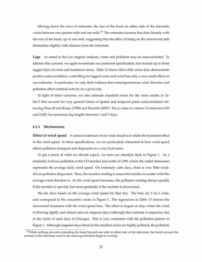
Moving down the rows of estimates, the size of the band on either side of the interstate
varies between one-quarter mile and one mile.29 The estimates increase less than linearly with
the size of the band, up to one mile, suggesting that the effect of being on the downwind side
diminishes slightly with distance from the interstate.
Lags As noted in the Los Angeles analysis, crime and pollution may be autocorrelated. To
address this concern, we again re-estimate our preferred specification, but include up to three
lagged days of crime and treatment status. Table 12 shows that while crime does demonstrate
positive autocorrelation, controlling for lagged crime and wind has only a very small effect on
our estimates. In particular, we only find evidence that contemporaneous wind direction and
pollution affect criminal activity on a given day.
In light of these concerns, we also estimate standard errors for the main results in Ta-
ble 9 that account for very general forms of spatial and temporal panel autocorrelation fol-
lowing Driscoll and Kraay (1998) and Hoechle (2007). The p-value in column 3 is between 0.06
and 0.065, for maximum lag lengths between 1 and 7 days.
6.1.1 Mechanisms
Effect of wind speed A natural extension of our main result is to relate the treatment effect
to the wind speed. In these specifications, we are particularly interested in how wind speed
affects pollution transport and dispersion in a very local sense.
To get a sense of what we should expect, we turn our attention back to Figure 1. As a
reminder, it shows pollution at the CO monitor just north of I-290, where the radial dimension
represents the average daily wind speed. On extremely calm days, there is very little wind-
driven pollution dispersion. Thus, the monitor reading is somewhat similar no matter what the
average wind direction is. As the wind speed increases, the pollution reading decays quickly
if the monitor is upwind, but more gradually if the monitor is downwind.
We bin days based on the average wind speed for that day. The bins are 2 m/s wide,
and correspond to the concentric circles in Figure 1. The regressions in Table 13 interact the
downwind treatment with the wind speed bins. The effect is largest on days when the wind
is blowing lightly, and almost zero on stagnant days (although that estimate is imprecise due
to the rarity of such days in Chicago). This is very consistent with the pollution pattern in
Figure 1. Although stagnant days (those in the smallest circle) are highly polluted, the pollution
29While nothing prevents extending the band beyond one mile to either side of the interstate, the bands around thesections of the interstate used in the main specification begin to overlap.
21
exposure on the north side of the interstate is elevated even when the wind blows mostly from
the north. On days in the second-smallest circle, the downwind neighborhood is exposed to
significantly more pollution than the upwind neighborhood. The effect grows again as the
wind picks up, but these are imprecisely estimated as such days are relatively rare.
These results bolster the case for a causal relationship between pollution and violent crime.
At the same time, they underscore the importance of interpreting the magnitude of our esti-
mates as a reduced form relationship, as measuring the exact difference in pollution treatment
is not straightforward.
Crime subcategories Although it is convenient to examine aggregated violent and property
crimes, there are substantial differences in the natures and costs of the different crimes. We can
further disaggregate the data and estimate effects for the individual index crimes. In doing so,
we sacrifice power, especially among the rarer crimes such as homicide. Still, the results are
informative.
Table 14 presents the results of estimating our preferred specification separately for the var-
ious violent crimes in our data. We estimate 7.8 and 3.4 percent increases in rape and homicide,
respectively, but these are not significantly different from zero. The estimated increase in vio-
lent crime appears to be driven by aggravated battery arrests. At the same time, the number
of aggravated assault arrests decreases. An assault is defined as “an unlawful attack by one
person upon another wherein the offender displays a weapon in a threatening manner, placing
someone in reasonable apprehension of receiving a battery.” A battery is defined “an unlawful
attack by one person upon another wherein the offender uses a weapon or the victim suffers
obvious severe or aggravated bodily injury involving apparent broken bones, loss of teeth, pos-
sible internal injury, severe laceration, or loss of consciousness.”30. That is, a battery subsumes
an assault in the case that actual bodily injury is sustained. One interpretation of these results
is that pollution causes a net increase in violent crime, but it also results in marginal assaults
escalating into batteries.
Breaking down the property crime (Table 15) results confirms that there is no effect within
any particular type of crime that is being obscured by an opposite response among another
type.
30Definitions of FBI index crimes are given at http://gis.chicagopolice.org/clearmap crime sums/crime types.html.
22
6.1.2 Results from an alternative identification strategy
To further test the robustness of our main results, we exploit a different source of variation
induced by the wind. In the main specification, we included route-side and route-date fixed
effects. Thus, our estimates came from the response of crime in a given neighborhood to being
downwind, relative to the corresponding upwind neighborhood on the same day.
In this alternative specification, we essentially use crime (and average wind exposure) at a
location on the same day of the year in other years as a control for crime at the location on the
day of interest. That is, when a given route-side is more consistently downwind on July 10th,
2011 than on the typical July 10th, do we see higher violent crime on that day? In the first three
columns, the treatment variable calculates the fraction of the day the wind was blowing to
that side of the road. In the last three columns, the treatment is continuous: the wind blowing
directly towards one side is a stronger treatment than wind blowing at an angle to the vector
of orthogonality.31 The sample size is larger than the main specification because we are able to
use all days in our data, rather than restricting our sample to only the days in which the wind
is blowing orthogonally to the interstate on average.
Table 16 presents the results. On a day that is “unusually downwind” for that calendar
date, a neighborhood experiences more violent crime. For a given route-side, a completely
upwind day will have 0.03 more violent crimes than a completely downwind day using the
binary treatment variable. The continuous treatment variable ranges from -1 to 1, so it predicts
that a completely upwind day will have roughly 0.035 more violent crimes than a completely
downwind day.
These signs and magnitudes are remarkably similar to those in our main specification, even
though the exogenous variation in wind exposure is coming from a comparison with different
implicit control groups. We take this as evidence that our main causal result is not simply an
artifact of our primary specification.
6.1.3 Placebo Tests
As a final piece of evidence, we consider a placebo test of our identification strategy. To moti-
vate the placebo test, consider the following thought exercise. Suppose we did not know ex ante
the latitude at which I-290 cuts straight east/west through the city of Chicago. We could esti-
31Specifically, we calculate the cosine of the difference between the wind angle and the direction orthogonal to theinterstate that makes the side of interest downwind. Thus, for an orthogonally upwind side-day, the variable takes avalue of cos (π) = −1. For a fully downwind side-day, the variable takes a value of cos (0) = 1. A day with an averagedirection parallel to the interstate takes on a value cos (π/2) = 0.
23

mate downwind coefficients from our model at a number of different latitudes. We could then
examine whether the effect on violent crime of being downwind was greatest at the latitude
of I-290. If we found large effects at alternative latitudes, we might worry that our downwind
treatment was capturing effects other than pollution from mobile sources.
To conduct the exercise, we focus on the band of crimes at similar longitudes to the crimes in
our sample set for I-290, but extending far north and south of I-290. Figure 6 maps the latitude
and longitudes of the crimes we use for the falsification test in green and the location of the
interstates in red. Moving from the south to the north in one mile increments, we consider
alternative latitudes with which we conduct a t-test equivalent to the main specification in
equation (3). For each latitude, we calculate the daily difference in violent crimes one mile
north of the latitude and one mile south of the latitude. We then test whether the differential at
that latitude is greater on days when the wind blows north than when the wind blows south.
Figure 7 plots the difference in the north-south violent crime differential on days when
the wind is blowing to north rather than the south at each alternative latitude, adjusted for
the fact that when the wind is blowing to the south, the pollution “treatment” applies to the
southern-side of the latitude. The interpretation is identical to the interpretation of the down-
wind treatment in column 2 of Table 9, although this exercise only examines one of the seven
interstate segments.
Three points in particular stand out in Figure 7. First, the maximum estimated downwind
effect (in the center of the graph) is exactly at the latitude that I-290 cuts east-west through
Chicago. Second, just to the right of the peak, corresponding to a latitude slightly of I-290, we
find the lowest estimated value for the downwind effect. When we consider an alternative lat-
itude just north of I-290, winds from the south blow pollution from the road onto the south side
of the alternative latitude and reverse the sign of the downwind effect. Relative to the alterna-
tive latitude, pollution is from I-290 falls on the upwind side. The sharp rebound at latitudes
just north of the minimum estimated downwind effect is also reassuring. This suggests that
the source of pollution is very local to the latitude at which I-290 cuts through Chicago from
east to west and disperses at latitudes further north. Finally, the second highest peak on the
graph (at a latitude of roughly 41.84) is on the northern side of I-55 as it exits the sample region
of the falsification test.
24
7 Broader Implications
We establish evidence that increases in ambient pollution causes an uptick in violent criminal
activity. This has two clear policy consequences. First, a Pigouvian tax or external cost estimate
for local pollutants excluding the cost of crime would be understated. Second, the cognitive
and behavioral effects of pollution exposure may include a much wider range of outcomes and
decisions than previously thought.
Although we estimate that the effect of pollution on crime is modest in percentage terms,
the annual aggregate costs of crime are enormous. Estimates from the literature vary in mag-
nitude: more conservative estimates suggest crime imposes external costs of several hundred
billion dollars per year annually in the U.S., while the upper end of estimates (e.g., Anderson,
1999) puts the aggregate cost of crime at over one trillion dollars annually.
Using our estimates of the effects of pollution on crime in Chicago, we compute a back-of-
the-envelope estimate of the cost of mobile pollution-induced crime. We apply cost of crime
estimates from the literature, assuming that all the additional crimes are assaults and batteries
to be conservative.32 Then we scale our estimates up to the size of the urbanized population
of the United States. Under these assumptions, the annual cost to the United States amounts
to $178 million per year. For comparison, Currie and Walker (2011) produce a back-of-the-
envelope estimate that pre-term births due to traffic congestion carry costs of $444 million per
year.
Willingness-to-pay estimates from the stated and revealed preference literatures can also
help describe the general magnitude of the effect. Bishop and Murphy (2011) apply a hedonic
model to LA housing data, and estimate that mean willingness to pay for a 10% in violent crime
is 472 USD (2010) per household per year. Taking the 6.1% increase from our LA estimates, this
suggests a willingness to pay of somewhere around 250-300 USD (2010) to eliminate the crime
we estimate to be pollution-induced.
Although we cannot put an exact number on the cost of pollution-induced violent crime,
it is robustly positive, and appears to be economically significant. Translating any of these
calculations directly to the appropriate adjustment to Pigouvian tax is difficult, given that we
identify the effect off of the difference between ”good” and ”bad” air days. Still, they demon-
strate that the pollution-crime externality is non-trivial, and should be considered in future
research and policy decisions.
We do not take a stand on the exact underlying mechanism, but our results suggest that air
32Details of the calculation are in Appendix A.3.
25

pollution may impact behavior in economically-meaningful ways much more broad than pre-
viously considered. Although we focus on violent criminal activity as an outcome, the potential
underlying loss of control and increased impulsivity may be related to other economically im-
portant decisions, summarized broadly in Kahneman (2011). These results also provide insight
into potential behavioral explanations behind lost productivity and performance found by pre-
vious studies. Finally, we see our results as complementary to the literature on the cognitive
effects of poverty (e.g., Mani et al., 2013; Schilbach et al., 2016), in which cognitive load and
stress lead to poor decisionmaking. Pollution exposure may have similar effects, which adds
an additional dimension of concern to policy debates about environmental justice and high
levels of pollution in the developing world.
8 Conclusion
The primary contribution of this paper is to identify a causal relationship between short-run
variation in air pollution and violent crime. Our approach exploits variation in air quality
induced by naturally occurring changes in wind direction in two heavily-populated parts of
the United States. In the Los Angeles basin, a wind blowing from the west “treats” only some
communities with polluted air; this is determined by the specifics of local topography. In
Chicago, wind orthogonal to a major interstate such as the I-290 treats those neighborhoods on
the downwind side with pollution from highway users, but not those upwind. Each setting
lends itself to a design similar to a difference-in-differences estimator.
The analyses in both Los Angeles and Chicago provide evidence of a causal link from ele-
vated air pollution in an area to higher same-day incidence of violent crime in that area. The
effect can persist from one calendar day to the next, though the size of the lagged treatment
effect is much smaller or zero. We find no evidence of any such link for property crime, so
this appears to be a story about violence, not criminality more generally, consistent with the
literature in other disciplines on air pollution and aggression.
The size of the estimated effects are substantial. In our preferred specification in Los An-
geles a treated community experiences a 6.14% increase in the incidence of violent crime. In
Chicago, violent crime increases by 2.2% in a neighborhood on the downwind side of a major
interstate. Back of the envelope calculations based on these magnitudes suggest that the cost
to society is meaningful compared to other outcomes studied in the external costs literature.
To our knowledge, this is the first paper documenting a causal relationship between ambi-
ent pollution and crime. As such it is appropriate, within each setting, to subject the central
26

estimates to a wide variety of robustness and falsification tests. However, we also contend
that each setting acts to corroborate the results of the other, and that the pair of case studies
– generating congruent results – are more persuasive in combination than either would be in-
dividually. Concerns regarding idiosyncratic threats to identification that might arise in one
setting can be allayed by the consistency of results from the other.
While we are unable to provide positive evidence on the underlying mechanism, our re-
sults suggest that air pollution may impact behavior in economically-meaningful ways much
more broad than previously considered. From a policy standpoint, the analysis points to an
additional social cost of air pollution. Estimates of the marginal social cost of air pollutants
that ignore it can be expected to understate the social benefit of pollution control interventions.
Thus, benefit-cost analysis based on such estimates will prescribe environmental policies that
are insufficiently stringent.
More generally our work contributes to the growing recognition that, in addition to the
well-understood health benefits, a clean natural environment contributes to a much wider
range of positive economic and social outcomes.
27
References
Amitai, Y., Zlotogorski, Z., Golan-Katzav, V., Wexler, A., and Gross, D. (1998). Neuropsycholog-
ical impairment from acute low-level exposure to carbon monoxide. Archives of Neurology,
55(6):845–848.
Anderson, C. A. and Bushman, B. J. (2002). Human aggression. Annual Review of Psychology,
53:27–51.
Anderson, D. A. (1999). The aggregate burden of crime*. The Journal of Law and Economics,
42(2):611–642.
Baron, R. A. and Bell, P. A. (1976). Aggression and heat: The influence of ambient temperature,
negative affect, and a cooling drink on physical aggression. Journal of Personality and Social
Psychology, 33(3):245.
Beatty, T. K. and Shimshack, J. P. (2014). Air pollution and children’s respiratory health: A
cohort analysis. Journal of Environmental Economics and Management, 67(1):39–57.
Birger, M., Swartz, M., Cohen, D., Alesh, Y., Grishpan, C., and Kotelr, M. (2003). Aggression:
The testosterone-serotonin link. Journal of Israel Medical Association, 5(9):653–658.
Bishop, K. C. and Murphy, A. D. (2011). Estimating the willingness to pay to avoid violent
crime: A dynamic approach. American Economic Review, 101(3):625–629.
Blumenthal, D., White, W., and Smith, T. (1978). Anatomy of a los angeles smog episode: Pollu-
tant transport in the daytime sea breeze regime. Atmospheric Environment (1967), 12(4):893–
907.
Briere, J., Downes, A., and Spensley, J. (1983). Summer in the city: Urban weather conditions
and psychiatric emergency-room visits. Journal of Abnormal Psychology, 92(1):77–80.
Coccaro, E. F., Sripada, C. S., Yanowitch, R. N., and Phan, K. L. (2011). Corticolimbic function
in impulsive aggressive behavior. Biological Psychiatry, 69(12):1153–1159.
Cohen, L. E. and Felson, M. (1979). Social change and crime rate trends: A routine activity
approach. American Sociological Review, 44:588–608.
Crockett, M. J., Apergis-Schoute, A., Herrmann, B., Lieberman, M. D., Muller, U., Robbins,
T. W., and Clark, L. (2013). Serotonin modulates striatal responses to fairness and retaliation
in humans. Journal of Neuroscience, 33(8):3505–3513.
28

Currie, J. and Walker, R. (2011). Traffic congestion and infant health: Evidence from e-zpass.
American Economic Journal: Applied Economics, 3(1):65–90.
Dabbs Jr, J. M., Carr, T. S., Frady, R. L., and Riad, J. K. (1995). Testosterone, crime, and misbe-
havior among 692 male prison inmates. Personality and Individual Differences, 18(5):627–633.
Donnerstein, E. and Wilson, D. W. (1976). Effects of noise and perceived control on ongoing
and subsequent aggressive behavior. Journal of Personality and Social Psychology, 34(5):774.
Driscoll, J. and Kraay, A. (1998). Consistent covariance matrix estimation with spatially depen-
dent data. Review of Economics and Statistics, 80(4):549–560.
Faustman, W. O., Ringo, D. L., and Faull, K. F. (1993). An association between low levels
of 5-HIAA and HVA in cerebrospinal fluid and early mortality in a diagnostically mixed
psychiatric sample. British Journal of Psychiatry, 163(4):519–521.
Frankle, W. G., Lombardo, I., New, A. S., Goodman, M., Talbot, P. S., Huang, Y., Hwang, D.-R.,
Slifstein, M., Curry, S., Abi-Dargham, A., et al. (2005). Brain serotonin transporter distri-
bution in subjects with impulsive aggressivity: A positron emission study with [11C] McN
5652. American Journal of Psychiatry, 162(5):915–923.
Gonzalez-Guevara, E., Martınez-Lazcano, J. C., Custodio, V., Hernandez-Ceron, M., Rubio, C.,
and Paz, C. (2014). Exposure to ozone induces a systemic inflammatory response: Possible
source of the neurological alterations induced by this gas. Inhalation Toxicology, 26(8):485–
491.
Hanna, R. and Oliva, P. (2015). The effect of pollution on labor supply: Evidence from a natural
experiment in mexico city. Journal of Public Economics, 122(1):68–79.
Hansenne, M., Reggers, J., Pinto, E., Kjiri, K., Ajamier, A., and Ansseau, M. (1999). Tempera-
ment and Character Inventory (TCI) and depression. Journal of Psychiatric Research, 33(1):31–
36.
Hoechle, D. (2007). Robust standard errors for panel regressions with cross-sectional depen-
dence. The Stata Journal, 7(3):281–312.
Ito, K. and Zhang, S. (2016). Willingness to pay for clean air: Evidence from air purifier markets
in china. Technical report, National Bureau of Economic Research.
29

Jacob, B., Lefgren, L., and Moretti, E. (2007). The dynamics of criminal behavior evidence from
weather shocks. Journal of Human Resources, 42(3):489–527.
Kahneman, D. (2011). Thinking, fast and slow. Macmillan.
Kinawy, A. A. (2009). Impact of gasoline inhalation on some neurobehavioural characteristics
of male rats. BMC Physiology, 9(1):21–31.
Krueger, A. P., Andriese, P. C., and Kotaka, S. (1963). The biological mechanism of air ion
action: The effect of CO2+ in inhaled air on the blood level of 5-hydroxytryptamine in mice.
International Journal of Biometeorology, 7(1):3–16.
Lavy, V., Ebenstein, A., and Roth, S. (2014). The impact of short term exposure to ambient air
pollution on cognitive performance and human capital formation. Technical report, National
Bureau of Economic Research.
Levesque, S., Lull, M. E., Taetzsch, T., Kodavanti, U., Stadler, K., Wagner, A., Johnson, J. A.,
Duke, L., Kodavanti, P., Surace, M. J., et al. (2011). Diesel exhaust activates & primes mi-
croglia: Air pollution, neuroinflammation, & regulation of dopaminergic neurotoxicity. En-
vironmental Health Perspectives, 119(3):1149–1155.
Lim, Y.-H., Kim, H., Kim, J. H., Bae, S., Park, H. Y., and Hong, Y.-C. (2012). Air pollution and
symptoms of depression in elderly adults. Environmental Health Perspectives, 120(7):1023–
1028.
Lu, R., Turco, R., Stolzenbach, K., Friedlander, S., Xiong, C., Schiff, K., Tiefenthaler, L., and
Wang, G. (2003). Dry deposition of airborne trace metals on the los angeles basin and adja-
cent coastal waters. Journal of Geophysical Research: Atmospheres, 108(D2).
Lu, R. and Turco, R. P. (1994). Air pollutant transport in a coastal environment. part I: Two-
dimensional simulations of sea-breeze and mountain effects. Journal of the Atmospheric Sci-
ences, 51(15):2285–2308.
Lu, R. and Turco, R. P. (1996). Ozone distributions over the los angeles basin: Three-
dimensional simulations with the smog model. Atmospheric Environment, 30(24):4155–4176.
Maney, D. L. and Goodson, J. L. (2011). Neurogenomic mechanisms of aggression in songbirds.
Advances in Genetics, 75(1):83–119.
30
Mani, A., Mullainanathan, S., Shafir, E., and Zhao, J. (2013). Poverty impedes cognitive func-
tion. Science, 341(6149):976–980.
Matsueda, R. L. and Anderson, K. (1998). The dynamics of delinquent peers and delinquent
behavior. Criminology, 36(2):269–308.
McCarty, M. (2014). Good news: SoCal’s air is better. Bad news: It’s still the worst in
the US. http://www.scpr.org/news/2014/04/30/43876/southern-california-among-most-
polluted-regions-in/. Last accessed on Mar 25, 2015.
McCollister, K. E., French, M. T., and Fang, H. (2010). The cost of crime to society: New crime-
specific estimates for policy and program evaluation. Drug and Alcohol Dependence, 108:98–
109.
Moretti, E. and Neidell, M. (2011). Pollution, health, and avoidance behavior evidence from
the ports of los angeles. Journal of Human Resources, 46(1):154–175.
Murphy, S. R., Schelegle, E. S., Miller, L. A., Hyde, D. M., and Van Winkle, L. S. (2013). Ozone
exposure alters serotonin and serotonin receptor expression in the developing lung. Toxico-
logical Sciences, 134(1):168–179.
Nattero, G. and Enrico, A. (1996). Outdoor pollution and headache. Headache, 36:243–245.
Nevin, R. (2007). Understanding international crime trends: The legacy of preschool lead ex-
posure. Environmental Research, 104(3):315–336.
Paz, C. and Huitron-Resendiz, S. (1996). The effects of ozone exposure on the sleep-wake cycle
and serotonin contents in the pons of the rat. Neuroscience Letters, 204(1):49–52.
Polakovic, G. (2002). Finally tackling L.A.’s worst air polluter. Los Angeles Times. Last accessed
on July 26, 2016.
Rammal, H., Bouayed, J., Younos, C., and Soulimani, R. (2008). Evidence that oxidative stress is
linked to anxiety-related behaviour in mice. Brain, Behavior, and Immunity, 22(8):1156–1159.
Ranson, M. (2014). Crime, weather, and climate change. Journal of Environmental Economics and
Management, 67(3):274–302.
Reyes, J. W. (2007). Environmental policy as social policy? the impact of childhood lead expo-
sure on crime. The BE Journal of Economic Analysis & Policy, 7(1).
31

Rotton, J. (1983). Affective and cognitive consequences of malodorous pollution. Basic and
Applied Social Psychology, 4(2):171–191.
Rotton, J., Barry, T., Frey, J., and Soler, E. (1978). Air pollution and interpersonal attraction1.
Journal of Applied Social Psychology, 8(1):57–71.
Rotton, J. and Frey, J. (1984). Psychological costs of air pollution: Atmospheric conditions,
seasonal trends, and psychiatric emergencies. Population and Environment, 7(1):3–16.
Schilbach, F., Schofield, J., and Mullainanathan, S. (2016). The psychological lives of the poor.
American Economic Review, 106(5):435–440.
Schlenker, W. and Walker, W. R. (2016). Airports, air pollution, and contemporaneous health.
Review of Economic Studies, 83(2):768–809.
Schultz, P. and Warner, T. T. (1982). Characteristics of summertime circulations and pollutant
ventilation in the los angeles basin. Journal of Applied Meteorology, 21(5):672–682.
Siegel, J. Z. and Crockett, M. J. (2013). How serotonin shapes moral judgment and behavior.
Annals of the New York Academy of Sciences, 1299(1):42–51.
Strahilevitz, M. (1977). Air pollutants and the admission rate of psychiatric patients. American
Journal of Pschiatry, 136(2):205–207.
Stretesky, P. B. and Lynch, M. J. (2004). The relationship between lead and crime. Journal of
Health and Social Behavior, 45(2):214–229.
Szyszkowicz, M. (2007). Air pollution and emergency department visits for depression in
edmonton, canada. International Journal of Occupational Medicine and Environmental Health,
20(3):241–245.
Szyszkowicz, M., Willey, J. B., Grafstein, E., Rowe, B. H., and Colman, I. (2010). Air pollution
and emergency department visits for suicide attempts in vancouver, canada. Environmental
Health Insights, 4:79–86.
Uboh, F., Akpanabiatu, M., Ekaidem, I., Ebong, P., and Umoh, I. (2007). Effect of inhalation
exposure to gasoline on sex hormones profile in Wistar albino rats. International Journal of
Romanian Society of Endocrinology, 3(1):23–30.
United States Census Bureau (2010). 2010 census.
32
Van Berlo, D., Albrecht, C., Knaapen, A. M., Cassee, F. R., Gerlofs-Nijland, M. E., Kooter, I. M.,
Palomero-Gallagher, N., Bidmon, H.-J., van Schooten, F.-J., Krutmann, J., et al. (2010). Com-
parative evaluation of the effects of short-term inhalation exposure to diesel engine exhaust
on rat lung and brain. Archives of Toxicology, 84(7):553–562.
Yang, A. C., Tsai, S.-J., and Huang, N. E. (2011). Decomposing the association of completed
suicide with air pollution, weather, and unemployment data at different time scales. Journal
of Affective Disorders, 129(1):275–281.
Zivin, J. G. and Neidell, M. (2009). Days of haze: Environmental information disclosure
and intertemporal avoidance behavior. Journal of Environmental Economics and Management,
58(2):119–128.
Zivin, J. G. and Neidell, M. (2012). The impact of pollution on worker productivity. The Ameri-
can Economic Review, 102(7):3652–3673.
33
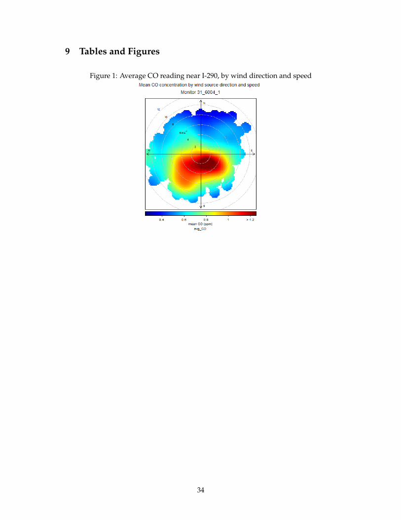
9 Tables and Figures
Figure 1: Average CO reading near I-290, by wind direction and speed
34

Figure 2: Distribution of wind source direction
Panel A: Los Angeles Panel B: Chicago
Figure 3: Los Angeles from the southwest
35

Figure 4: Positive vs. Negative AQSs
36

Figure 5: Chicago: Sample set for interstate identification strategy
Figure 6: Chicago: Sample set for falsification test
37

Figure 7: Chicago: North-south crime differential, alternative latitudes
Note: The y-axis reports the difference in the number of violent crimes one mile north ver-sus one mile south of the latitude reported on days when the wind is blowing northernlyrather than southernly. Northernly and southernly are defined as within 60 degrees ofnorth and south, respectively. The solid line denotes the point estimate of the differenceand the dashed lines denote the upper and lower bounds of the 95% confidence intervalof the t-test. The vertical lines denote the latitudes of I-290 and the average latitude ofI-55.
38
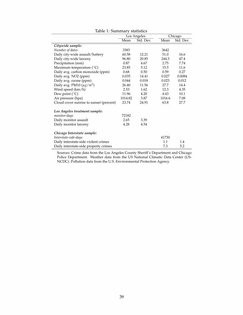
Table 1: Summary statisticsLos Angeles Chicago
Mean Std. Dev. Mean Std. Dev.Citywide sample:Number of dates 3383 3642Daily city-wide assault/battery 60.58 12.21 51.0 16.6Daily city-wide larceny 96.80 20.85 244.3 47.4Precipitation (mm) 0.87 4.67 2.75 7.74Maximum temperature (◦C) 23.85 5.12 15.5 11.6Daily avg. carbon monoxide (ppm) 0.68 0.50 0.59 0.27Daily avg. NO2 (ppm) 0.035 14.41 0.027 0.0084Daily avg. ozone (ppm) 0.044 0.018 0.023 0.012Daily avg. PM10 (µg/m3) 26.40 11.56 27.7 14.4Wind speed (km/h) 2.53 1.62 12.3 4.35Dew point (◦C) 11.96 4.20 4.43 10.1Air pressure (hpa) 1014.82 3.87 1016.6 7.08Cloud cover sunrise to sunset (percent) 23.74 24.91 63.8 27.7
Los Angeles treatment sample:monitor-days 72182Daily monitor assault 2.65 3.39Daily monitor larceny 4.28 4.54
Chicago Interstate sample:Interstate-side-days 41730Daily interstate-side violent crimes 1.1 1.4Daily interstate-side property crimes 7.3 5.2
Sources: Crime data from the Los Angeles County Sheriff’s Department and ChicagoPolice Department. Weather data from the US National Climatic Data Center (US-NCDC). Pollution data from the U.S. Environmental Protection Agency.
39
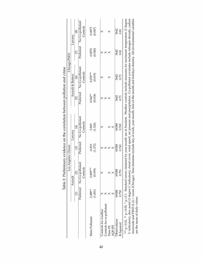
Tabl
e2:
Prel
imin
ary
evid
ence
onth
eco
rrel
atio
nbe
twee
npo
lluti
onan
dcr
ime
Los
Ang
eles
:Ozo
neC
hica
go:P
M10
Ass
ault
Larc
eny
Ass
ault
&Ba
tter
yLa
rcen
y(1
)(2
)(3
)(4
)(5
)(6
)(7
)(8
)Pr
efer
red
No
Co-
pollu
tant
Pref
erre
dN
oC
o-po
lluta
ntPr
efer
red
No
Co-
pollu
tant
Pref
erre
dN
oC
o-po
lluta
ntC
ontr
ols
Con
trol
sC
ontr
ols
Con
trol
s
Mai
nPo
lluta
nt2.
488*
*2.
809*
**-0
.810
0.86
90.
042*
*0.
078*
**0.
0070
-0.0
073
(1.0
01)
(0.9
39)
(1.3
72)
(1.3
24)
(0.0
18)
(0.0
19)
(0.0
40)
(0.0
47)
Con
trol
sfo
rw
eath
erX
XX
XX
XX
XC
ontr
ols
for
co-p
ollu
tant
XX
XX
Tim
eFE
XX
XX
XX
XX
AQ
SfF
EX
XX
XO
bser
vati
ons
6938
869
388
6938
869
388
3642
3642
3642
3642
R-S
quar
ed0.
750
0.75
10.
743
0.76
50.
730.
730.
810.
81
***
p<
0.01
,**
p<
0.05
,*p<
0.1.
Stan
dard
erro
rscl
uste
red
byye
ar-m
onth
are
inbr
acke
ts.
Wea
ther
cont
rols
incl
ude
mea
sure
sfo
rm
axim
umte
mpe
ratu
re(3
degr
eeC
indi
cato
rs),
dew
poin
t(3
degr
eeC
indi
cato
rs),
clou
dco
ver,
win
dsp
eed,
air
pres
sure
and
prec
ipit
atio
n.C
o-po
lluta
ntco
vari
ates
incl
ude
nitr
ogen
diox
ide,
carb
onm
onox
ide
and
PM10
(LA
)/oz
one
(Chi
cago
).Ti
me
dum
mie
sin
clud
eda
yof
wee
k,ye
ar-m
onth
,firs
t-of
-the
-mon
than
dho
liday
sdu
mm
y.A
llen
viro
nmen
talv
aria
bles
are
the
mea
nof
daily
valu
es.
40

Tabl
e3:
LA:E
ffec
tofW
este
rly
Win
don
Ozo
neby
AQ
S(1
)(2
)(3
)(4
)(5
)(6
)(7
)(8
)A
zusa
Gle
ndor
aSa
wte
lleBu
rban
kLA
Dow
ntow
nR
esed
aLy
nwoo
dC
ompt
onW
est
0.00
126∗
∗0.
0012
10.
0004
580.
0009
560.
0004
580.
0010
6∗∗
0.00
585∗
∗0.
0012
6∗∗∗
(0.0
0058
4)(0
.001
02)
(0.0
0033
0)(0
.001
00)
(0.0
0043
7)(0
.000
454)
(0.0
0294
)(0
.000
447)
Obs
erva
tion
s29
0029
0029
0029
0029
0029
0017
5013
70R
-Squ
ared
0.74
30.
784
0.59
50.
766
0.71
40.
732
0.74
90.
707
(9)
(10)
(11)
(12)
(13)
(14)
(15)
(16)
Pico
Riv
era
Pom
ona
Pasa
dena
Long
Beac
hLo
wer
Wes
tsid
ePl
aya
Del
Rey
Sant
aC
lari
taLa
ncas
ter
Wes
t-0
.001
35∗∗
-0.0
0045
80.
0052
7∗∗
0.00
224∗
∗∗-0
.000
783
-0.0
0300
∗∗∗
-0.0
0123
∗∗∗
0.00
527∗
∗
(0.0
0062
1)(0
.000
471)
(0.0
0225
)(0
.000
338)
(0.0
0060
1)(0
.001
12)
(0.0
0041
7)(0
.002
20)
Obs
erva
tion
s26
0029
0029
0029
0029
0029
0014
3029
00R
-Squ
ared
0.76
50.
744
0.80
00.
723
0.66
20.
632
0.54
60.
737
(17)
(18)
(19)
(20)
(21)
(22)
Lebe
cA
nahe
imM
esa
Verd
eIr
vine
LaH
abra
Thou
sand
Oak
sW
est
0.00
0197
-0.0
0006
91-0
.001
40∗∗
∗-0
.000
419
-0.0
0123
∗∗-0
.000
148
(0.0
0038
2)(0
.000
342)
(0.0
0053
9)(0
.000
552)
(0.0
0062
2)(0
.000
555)
Obs
erva
tion
s51
329
0013
1829
0029
0029
00R
-Squ
ared
0.77
60.
727
0.65
40.
563
0.58
30.
722
Con
trol
sfo
rw
eath
erX
XX
XX
XX
XTi
me
FEX
XX
XX
XX
X
***
p<
0.01
,**
p<
0.05
,*p<
0.1.
Dep
ende
ntva
riab
leis
ozon
e.St
anda
rder
rors
clus
tere
dby
year
-mon
thar
ein
brac
kets
.W
eath
erco
ntro
lsin
clud
em
easu
res
for
max
imum
tem
pera
ture
(3de
gree
Cin
dica
tors
),de
wpo
int(
3de
gree
Cin
dica
tors
),cl
oud
cove
r,w
ind
spee
d,ai
rpr
essu
rean
dpr
ecip
-it
atio
n.Ti
me
dum
mie
sin
clud
eda
yof
wee
kan
dye
ar-m
onth
.All
envi
ronm
enta
lvar
iabl
esar
eth
em
ean
ofda
ilyva
lues
.∗
sign
ifica
ntat
10%
∗∗si
gnifi
cant
at5%
∗∗∗
sign
ifica
ntat
1%.
41

Table 4: LA: Assault(1) (2) (3) (4)
Treatment (West*Location Dummy) 0.162*** 0.242*** 0.175*** 0.0919***(0.0302) (0.0605) (0.0405) (0.0352)
Controls for weather XDate FE X XAQS FE X X X XObservations 72182 72182 72182 62339R-Squared 0.748 0.725 0.728 0.728
Notes: *** p<0.01, ** p<0.05, * p<0.1. Standard errors clustered by year-monthare in brackets. Weather controls include measures for maximum temperature(3 degree C indicators), dew point (3 degree C indicators), cloud cover, windspeed, air pressure and precipitation. Co-pollutant covariates include PM10,nitrogen dioxide and carbon monoxide. Column 4 excludes port monitoringstations including AQS numbers (7), (8), (12) and (13).
Table 5: LA: Larceny(1) (2) (3)
Treatment (West*Location Dummy) 0.0625 0.0518 0.0612(0.0504) (0.0628) (0.0489)
Controls for weather XDate FE XAQS FE X X XObservations 72182 72182 72182R-Squared 0.742 0.721 0.722
Notes: *** p<0.01, ** p<0.05, * p<0.1. Standard errors clustered byyear-month are in brackets. Weather controls include measures formaximum temperature (3 degree C indicators), dew point (3 degreeC indicators), cloud cover, wind speed, air pressure and precipita-tion. Co-pollutant covariates include PM10, nitrogen dioxide andcarbon monoxide. All environmental variables are the mean of dailyvalues.
Table 6: LA: Assault, by treatment angleAngle width 36 45 60 75 90Treatment 0.162*** 0.165*** 0.173*** 0.176*** 0.174***
(0.0302) (0.0306) (0.0303) (0.0296) (0.0297)Date FE X X X X XAQS FE X X X X XObservations 72182 72182 72182 72182 72182R-Squared 0.748 0.748 0.748 0.748 0.748
Notes: *** p<0.01, ** p<0.05, * p<0.1. Dependent variable is dailynumber of assaults. Standard errors clustered by year-month are inbrackets. Time dummies include date fixed effect. All environmen-tal variables are the mean of daily values.
42

Table 7: LA: Assault, including lagged variables(1) (2) (3) (4) (5) (6) (7)
Treatment 0.165*** 0.141*** 0.137*** 0.134*** 0.128*** 0.125*** 0.125***(0.0405) (0.0280) (0.0275) (0.0272) (0.0269) (0.0269) (0.0269)
Treatment, t-1 0.0951*** 0.0892*** 0.0848*** 0.0741** 0.0711** 0.0697**(0.0293) (0.0280) (0.0276) (0.0274) (0.0271) (0.0270)
Treatment, t-2 0.0303 0.0230 0.0160 0.00926 0.00719(0.0328) (0.0323) (0.0324) (0.0323) (0.0323)
Treatment, t-3 0.0396 0.0375 0.0328 0.0281(0.0241) (0.0240) (0.0241) (0.0240)
Number of crimes, t-1 0.0858** 0.0808*** 0.0787***(0.00755) (0.00702) (0.00691)
Number of crimes, t-2 0.0582*** 0.0553***(0.00668) (0.00656)
Number of crimes, t-3 0.0365***(0.00600)
Date FE X X X X X X XAQS FE X X X X X X XObservations 72182 72182 72182 72182 72182 72182 72182R-Squared 0.748 0.748 0.748 0.748 0.750 0.751 0.751
Notes: *** p<0.01, ** p<0.05, * p<0.1. Dependent variable is daily number of assaults. Standard errorsclustered by year-month are in brackets. All environmental variables are the mean of daily values.
Table 8: LA: Falsification(1) (2) (3) (4)
-100 +100 New York HoustonTreatment (West*Location Dummy) 0.0338 0.00268 0.00023 0.0234
(0.0310) (0.0294) (0.0410) (0.0313)Date FE X X X XAQS FE X X X XObservations 72182 72182 72182 72182R-Squared 0.748 0.749 0.778 0.698
Notes: *** p<0.01, ** p<0.05, * p<0.1. Dependent variable is daily number ofassaults. Standard errors clustered by year-month are in brackets. Time dummiesinclude date fixed effect. All environmental variables are the mean of daily values.
43

Table 9: Chicago: Violent crime downwind of inter-states
(1) (2) (3)Treatment (downwind) 0.0694*** 0.0231** 0.0234**
(0.0134) (0.0110) (0.0113)Route*Side FE X XRoute*Date FE X XRoute*Side Weather Interact. XObservations 41730 41730 41730R-Squared 0.000644 0.678 0.680
Notes: *** p<0.01, ** p<0.05, * p<0.1. Robust standard er-rors reported. The dependent variable is the number of crimeswithin one mile of one side of the interstate. A side of the inter-state is considered downwind if the average wind vector overthe course of the day is within 60 degrees of the vector orthog-onal to the direction of the interstate.
Table 10: Chicago: Property crime downwind of inter-states
(1) (2) (3)Treatment (downwind) 0.0108 -0.0101 -0.00457
(0.0509) (0.0295) (0.0304)Route*Side FE X XRoute*Date FE X XRoute*Side Weather Interact. XObservations 41730 41730 41730R-Squared 0.00000107 0.841 0.843
Notes: *** p<0.01, ** p<0.05, * p<0.1. Robust standard errorsreported. The dependent variable is the number of crimes withinone mile of one side of the interstate. A side of the interstate isconsidered downwind if the average wind vector over the courseof the day is within 60 degrees of the vector orthogonal to thedirection of the interstate.
44

Table 11: Chicago: Downwind violent crime, by treatment angleand distance from interstate
Angle width 36 45 60 75 9014 mile
Est. 0.0075 0.0112* 0.0137*** 0.0100** 0.0090**SE (0.0069) (0.0060) (0.0051) (0.0044) (0.0040)N 24760 31250 41730 51924 61362R2 0.579 0.582 0.588 0.587 0.588
12 mile
Est. 0.0145 0.0168* 0.0160** 0.0154** 0.0164***SE (0.0105) (0.0092) (0.0077) (0.0067) (0.0061)N 24760 31250 41730 51924 61362R2 0.637 0.639 0.642 0.641 0.64
1 mileEst. 0.0247 0.0235* 0.0234** 0.0166* 0.0152*SE (0.0153) (0.0134) (0.0113) (0.0099) (0.0090)N 24760 31250 41730 51924 61362R2 0.676 0.678 0.68 0.68 0.679
Notes: *** p<0.01, ** p<0.05, * p<0.1. Robust standard errors reported. Thedependent variable is the number of crimes within one mile of one side ofan interstate. All specifications include interstate*date fixed effects and inter-state*side fixed effects interacted with daily maximum temperature and totalprecipitation.
Table 12: Chicago: Downwind violent crime, including lagged variables(1) (2) (3) (4) (5) (6)
Treatment (downwind) 0.0234** 0.0263** 0.0256** 0.0255** 0.0262** 0.0261**(0.0113) (0.0121) (0.0121) (0.0121) (0.0121) (0.0121)
Downwind, t-1 -0.00491 -0.00272 -0.00260 -0.00352 -0.00296(0.00722) (0.00757) (0.00757) (0.00757) (0.00756)
Downwind, t-2 -0.00667 -0.00720 -0.00686 -0.00719(0.00708) (0.00736) (0.00736) (0.00735)
Downwind, t-3 0.00161 0.00172 0.00111(0.00709) (0.00708) (0.00708)
Number of crimes, t-1 0.0407*** 0.0372***(0.00846) (0.00846)
Number of crimes, t-2 0.0357***(0.00852)
Number of crimes, t-3 0.0382***(0.00868)
Route*Side FE X X X X X XRoute*Date FE X X X X X XRoute*Side Weather Interact. X X X X X XObservations 41730 41730 41730 41730 41730 41730R-Squared 0.680 0.680 0.680 0.680 0.681 0.682
Notes: *** p<0.01, ** p<0.05, * p<0.1. Robust standard errors reported. The dependent variable isthe number of crimes within one mile of one side of the interstate.
45
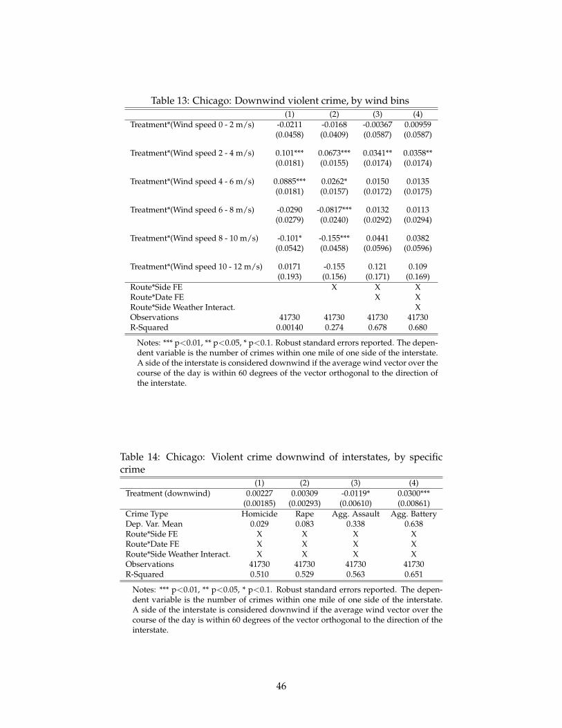
Table 13: Chicago: Downwind violent crime, by wind bins(1) (2) (3) (4)
Treatment*(Wind speed 0 - 2 m/s) -0.0211 -0.0168 -0.00367 0.00959(0.0458) (0.0409) (0.0587) (0.0587)
Treatment*(Wind speed 2 - 4 m/s) 0.101*** 0.0673*** 0.0341** 0.0358**(0.0181) (0.0155) (0.0174) (0.0174)
Treatment*(Wind speed 4 - 6 m/s) 0.0885*** 0.0262* 0.0150 0.0135(0.0181) (0.0157) (0.0172) (0.0175)
Treatment*(Wind speed 6 - 8 m/s) -0.0290 -0.0817*** 0.0132 0.0113(0.0279) (0.0240) (0.0292) (0.0294)
Treatment*(Wind speed 8 - 10 m/s) -0.101* -0.155*** 0.0441 0.0382(0.0542) (0.0458) (0.0596) (0.0596)
Treatment*(Wind speed 10 - 12 m/s) 0.0171 -0.155 0.121 0.109(0.193) (0.156) (0.171) (0.169)
Route*Side FE X X XRoute*Date FE X XRoute*Side Weather Interact. XObservations 41730 41730 41730 41730R-Squared 0.00140 0.274 0.678 0.680
Notes: *** p<0.01, ** p<0.05, * p<0.1. Robust standard errors reported. The depen-dent variable is the number of crimes within one mile of one side of the interstate.A side of the interstate is considered downwind if the average wind vector over thecourse of the day is within 60 degrees of the vector orthogonal to the direction ofthe interstate.
Table 14: Chicago: Violent crime downwind of interstates, by specificcrime
(1) (2) (3) (4)Treatment (downwind) 0.00227 0.00309 -0.0119* 0.0300***
(0.00185) (0.00293) (0.00610) (0.00861)Crime Type Homicide Rape Agg. Assault Agg. BatteryDep. Var. Mean 0.029 0.083 0.338 0.638Route*Side FE X X X XRoute*Date FE X X X XRoute*Side Weather Interact. X X X XObservations 41730 41730 41730 41730R-Squared 0.510 0.529 0.563 0.651
Notes: *** p<0.01, ** p<0.05, * p<0.1. Robust standard errors reported. The depen-dent variable is the number of crimes within one mile of one side of the interstate.A side of the interstate is considered downwind if the average wind vector over thecourse of the day is within 60 degrees of the vector orthogonal to the direction of theinterstate.
46

Table 15: Chicago: Property crime downwind of interstates, by specific crime(1) (2) (3) (4) (5)
Treatment (downwind) 0.00482 -0.00358 -0.00799 0.00298 -0.000807(0.0100) (0.0125) (0.0221) (0.0115) (0.00191)
Crime Type Robbery Burglary Larceny Gr. Theft Auto ArsonDep. Var. Mean 0.866 1.269 4.014 1.122 0.033Route*Side FE X X X X XRoute*Date FE X X X X XRoute*Side Weather Interact. X X X X XObservations 41730 41730 41730 41730 41730R-Squared 0.632 0.661 0.794 0.619 0.507
Notes: *** p<0.01, ** p<0.05, * p<0.1. Robust standard errors reported. The dependent vari-able is the number of crimes within one mile of one side of the interstate. A side of theinterstate is considered downwind if the average wind vector over the course of the day iswithin 60 degrees of the vector orthogonal to the direction of the interstate.
Table 16: Chicago: Downwind violent crime, alternative identification strategy(1) (2) (3) (4) (5) (6)
Treatment (binary) 0.0287** 0.0303** 0.0303**(0.0138) (0.0150) (0.0146)
Treatment (continuous) 0.0175* 0.0187* 0.0187*(0.00901) (0.00987) (0.00956)
Route*Side*Month FE X XRoute*Side*DoY FE X X X XCovariate Interactions X XObservations 61362 61362 61362 61362 61362 61362R-Squared 0.301 0.356 0.369 0.301 0.356 0.369
Notes: *** p<0.01, ** p<0.05, * p<0.1. Robust standard errors reported. The dependentvariable is the number of crimes within one mile of one side of the interstate. Binary andcontinuous variables constructed as described in Section 6.1.2.
47

A Appendix
A.1 Supplementary Tables and Figures - Los Angeles
A.1.1 Patterns of Crime in Los Angeles
Figure 8 shows hourly pattern in assault and larceny in Los Angeles. As shown assaults are
lowest in the early morning and tend to increase until midnight. Larceny theft crimes are also
at lowest rate in the early morning, they increase until evening but tend to decrease after that.
A feel for the seasonal variability in crime incidents is provided in Figure 9. Assaults are
concentrated in the hotter, more polluted months of May to August while the larcenies are more
up-and-down through the year. Normalizing crimes level in 2005 to 100, Figure 10 depicts the
annual trends in assaults and larcenies between 2005 and 2013. As it is clear, both group of
crimes have decreasing trend since 2005. Finally Figure 11 gives an impression of seasonality
of pollutants in Los Angeles. Ozone exhibits a strong seasonal pattern, with higher levels in
summer. CO exhibits the opposite pattern, with higher levels in winter.
Effects by wind power Not only wind direction but also wind speed plays an essential role
in determining pollution concentrations in a city. Although we control for wind speed in our
estimations, we test the effect of wind power in Table 17 by interacting our treatment variable
by wind bin. This allows us to compare a light west wind day with a strong west wind day.
As shown, winds between 4 - 6 meters per second have the larges, positive and statistically
significant effect on daily number of assaults in treated area. In addition, strong winds do not
have any significant effects on assault incidents.
Effects by season In Table 18 we interact our treatment variable by each season with refer-
ence season is winter. This is a suggestive approach allowing us to determine the most influen-
tial pollutant. As indicated, across all specifications point estimates are largest during summer
months suggesting ozone is the primary pollutant affecting assault incidents.
Effects by day of week Although we include date fixed effect in our estimation, our point
estimates show the individuals average behavior for a specific day. In Table 19 we interact our
treatment by day of week to allow the effect of treatment to vary by weekday versus week-
ends. As presented, our results are driven on weekends suggesting that the positive effect of
pollution on assaults can be augmented by higher number of people spending time in outdoor
activities on weekends.
48
A.2 Supplementary Tables and Figures - Chicago
A.2.1 Patterns of Crime in Chicago
Crime reports display certain temporal and seasonal regularities. As is clear from Figure 12,
reports of violent crime are lowest in the very early morning and steadily increase until mid-
night. Property crime reports also are lowest in the early morning, but tend to be higher during
the day than at night. In Figure 13, we present the average number of crimes for a given week
of the year to consider seasonality. Two things are worth noting here. First, the absolute mag-
nitude of property crime is roughly 6-7 times larger than that of violent crime. Second, the
seasonal patterns are slightly different. While violent crimes are approximately symmetrical
around their peak in the summer, property crimes tail off more slowly in the fall than they
rise in the spring. Finally, Figure 14 presents the annual trends in property and violent crimes
between 2001 and 2012. Each type of crime’s 2001 level is normalized to 100. Overall, violent
crime has declined more rapidly than property crime, although both varieties are far below
their 2001 levels.
In Figures 12 and 13, there are spikes in crime reports at midnight and in the first week of
the year. If one looks at the day of the month, there is also a spike on the first of the month.
Some of this is driven by the fact that the time and date in our data refer to the actual occurrence
of the crime, not the report. Thus, if someone waits to report a crime or forgets the time and
date exactly, they might be more likely to simply choose midnight or the first of the month.
Correspondence with the Chicago Police Department’s Research and Development Division
indicates that there is no official procedure that would otherwise be driving this phenomenon.
This effect is the largest for January 1, some of which could be driven by the New Year’s Eve
holiday. At any rate, we control for the 1st day of the month and year when appropriate in our
citywide regressions. In our analyses using detailed geographic coordinates, we are comparing
treatment and control areas within the same day, so any effect should be swept out.
The geographic patterns of property versus violent crime also differ from one another. The
heat maps in Figure 15 plot the density of property and violent crime throughout Chicago for
2001-2012. The grey lines denote the major interstates running through the city limits. The
shades are comparable only within a map; that is, an area on the violent crime map that is
darker than an area on the property crime map does not necessarily indicate that there are
more violent crimes in absolute terms. It simply means that the share of violent crimes that
occur in that area is greater than the share of property crimes. The poorer areas, such as the
South Side, and the westernmost portions of the West Side have experienced the most violent
49
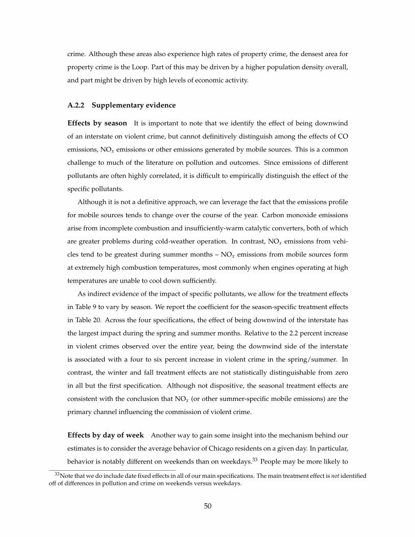
crime. Although these areas also experience high rates of property crime, the densest area for
property crime is the Loop. Part of this may be driven by a higher population density overall,
and part might be driven by high levels of economic activity.
A.2.2 Supplementary evidence
Effects by season It is important to note that we identify the effect of being downwind
of an interstate on violent crime, but cannot definitively distinguish among the effects of CO
emissions, NOx emissions or other emissions generated by mobile sources. This is a common
challenge to much of the literature on pollution and outcomes. Since emissions of different
pollutants are often highly correlated, it is difficult to empirically distinguish the effect of the
specific pollutants.
Although it is not a definitive approach, we can leverage the fact that the emissions profile
for mobile sources tends to change over the course of the year. Carbon monoxide emissions
arise from incomplete combustion and insufficiently-warm catalytic converters, both of which
are greater problems during cold-weather operation. In contrast, NOx emissions from vehi-
cles tend to be greatest during summer months – NOx emissions from mobile sources form
at extremely high combustion temperatures, most commonly when engines operating at high
temperatures are unable to cool down sufficiently.
As indirect evidence of the impact of specific pollutants, we allow for the treatment effects
in Table 9 to vary by season. We report the coefficient for the season-specific treatment effects
in Table 20. Across the four specifications, the effect of being downwind of the interstate has
the largest impact during the spring and summer months. Relative to the 2.2 percent increase
in violent crimes observed over the entire year, being the downwind side of the interstate
is associated with a four to six percent increase in violent crime in the spring/summer. In
contrast, the winter and fall treatment effects are not statistically distinguishable from zero
in all but the first specification. Although not dispositive, the seasonal treatment effects are
consistent with the conclusion that NOx (or other summer-specific mobile emissions) are the
primary channel influencing the commission of violent crime.
Effects by day of week Another way to gain some insight into the mechanism behind our
estimates is to consider the average behavior of Chicago residents on a given day. In particular,
behavior is notably different on weekends than on weekdays.33 People may be more likely to
33Note that we do include date fixed effects in all of our main specifications. The main treatment effect is not identifiedoff of differences in pollution and crime on weekends versus weekdays.
50
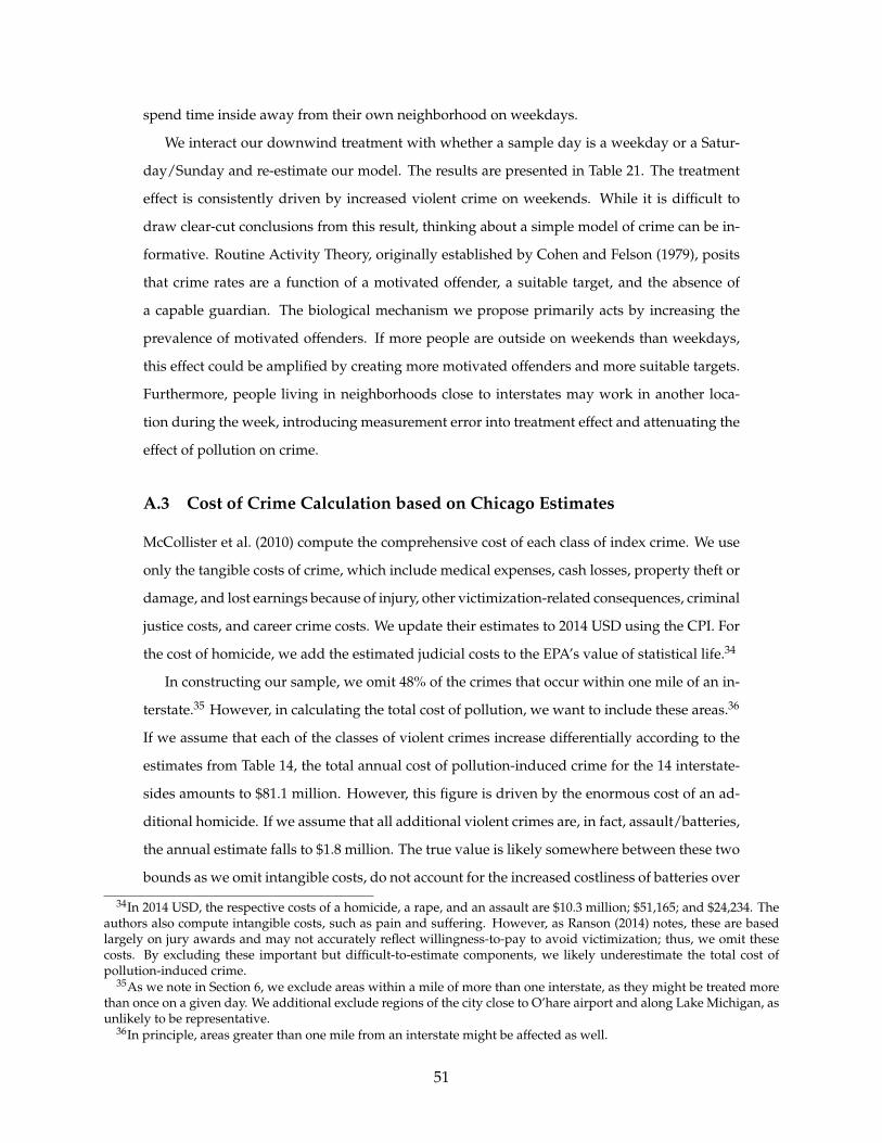
spend time inside away from their own neighborhood on weekdays.
We interact our downwind treatment with whether a sample day is a weekday or a Satur-
day/Sunday and re-estimate our model. The results are presented in Table 21. The treatment
effect is consistently driven by increased violent crime on weekends. While it is difficult to
draw clear-cut conclusions from this result, thinking about a simple model of crime can be in-
formative. Routine Activity Theory, originally established by Cohen and Felson (1979), posits
that crime rates are a function of a motivated offender, a suitable target, and the absence of
a capable guardian. The biological mechanism we propose primarily acts by increasing the
prevalence of motivated offenders. If more people are outside on weekends than weekdays,
this effect could be amplified by creating more motivated offenders and more suitable targets.
Furthermore, people living in neighborhoods close to interstates may work in another loca-
tion during the week, introducing measurement error into treatment effect and attenuating the
effect of pollution on crime.
A.3 Cost of Crime Calculation based on Chicago Estimates
McCollister et al. (2010) compute the comprehensive cost of each class of index crime. We use
only the tangible costs of crime, which include medical expenses, cash losses, property theft or
damage, and lost earnings because of injury, other victimization-related consequences, criminal
justice costs, and career crime costs. We update their estimates to 2014 USD using the CPI. For
the cost of homicide, we add the estimated judicial costs to the EPA’s value of statistical life.34
In constructing our sample, we omit 48% of the crimes that occur within one mile of an in-
terstate.35 However, in calculating the total cost of pollution, we want to include these areas.36
If we assume that each of the classes of violent crimes increase differentially according to the
estimates from Table 14, the total annual cost of pollution-induced crime for the 14 interstate-
sides amounts to $81.1 million. However, this figure is driven by the enormous cost of an ad-
ditional homicide. If we assume that all additional violent crimes are, in fact, assault/batteries,
the annual estimate falls to $1.8 million. The true value is likely somewhere between these two
bounds as we omit intangible costs, do not account for the increased costliness of batteries over
34In 2014 USD, the respective costs of a homicide, a rape, and an assault are $10.3 million; $51,165; and $24,234. Theauthors also compute intangible costs, such as pain and suffering. However, as Ranson (2014) notes, these are basedlargely on jury awards and may not accurately reflect willingness-to-pay to avoid victimization; thus, we omit thesecosts. By excluding these important but difficult-to-estimate components, we likely underestimate the total cost ofpollution-induced crime.
35As we note in Section 6, we exclude areas within a mile of more than one interstate, as they might be treated morethan once on a given day. We additional exclude regions of the city close to O’hare airport and along Lake Michigan, asunlikely to be representative.
36In principle, areas greater than one mile from an interstate might be affected as well.
51
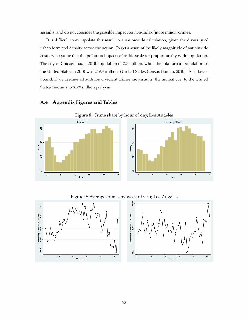
assaults, and do not consider the possible impact on non-index (more minor) crimes.
It is difficult to extrapolate this result to a nationwide calculation, given the diversity of
urban form and density across the nation. To get a sense of the likely magnitude of nationwide
costs, we assume that the pollution impacts of traffic scale up proportionally with population.
The city of Chicago had a 2010 population of 2.7 million, while the total urban population of
the United States in 2010 was 249.3 million (United States Census Bureau, 2010). As a lower
bound, if we assume all additional violent crimes are assaults, the annual cost to the United
States amounts to $178 million per year.
A.4 Appendix Figures and Tables
Figure 8: Crime share by hour of day, Los Angeles
Figure 9: Average crimes by week of year, Los Angeles
52
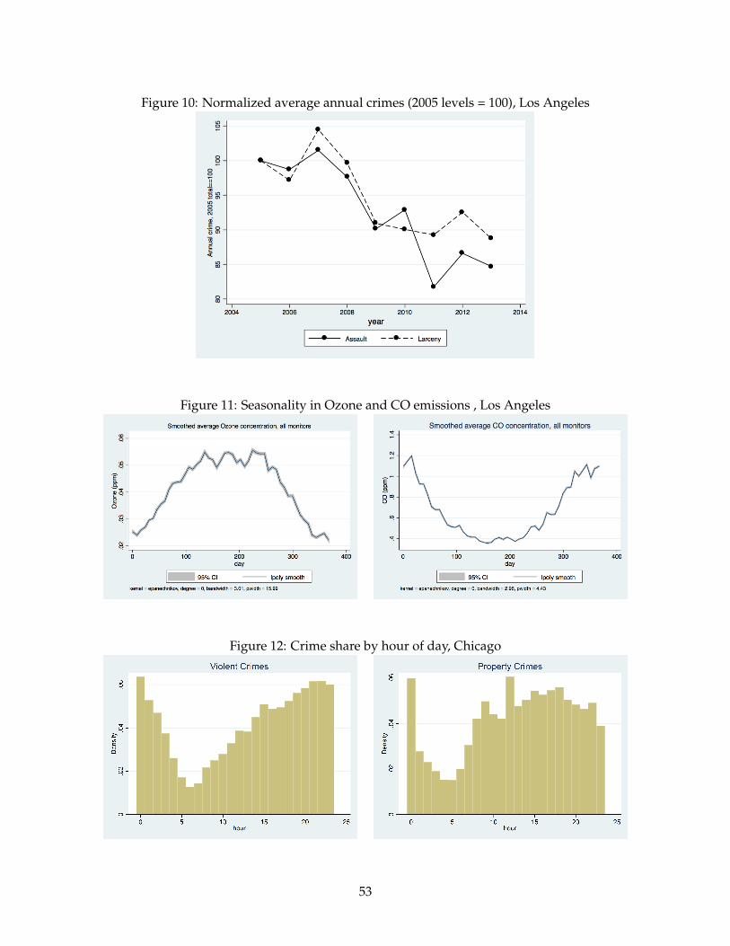
Figure 10: Normalized average annual crimes (2005 levels = 100), Los Angeles
Figure 11: Seasonality in Ozone and CO emissions , Los Angeles
Figure 12: Crime share by hour of day, Chicago
53
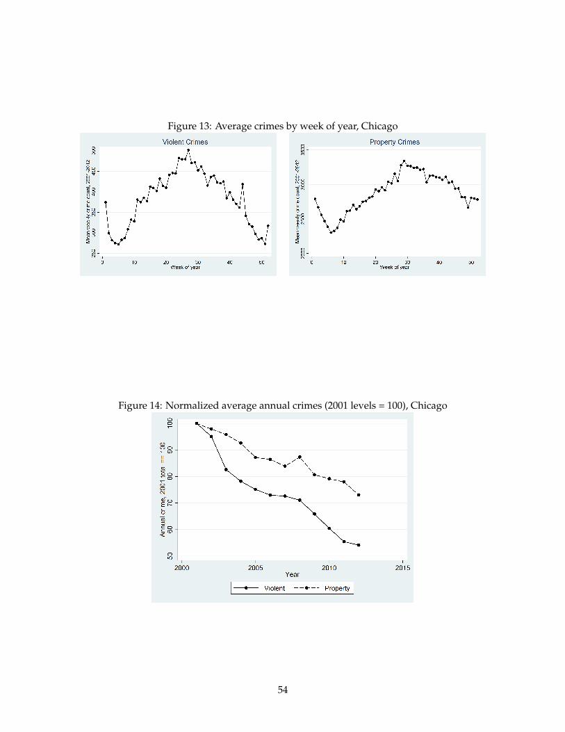
Figure 13: Average crimes by week of year, Chicago
Figure 14: Normalized average annual crimes (2001 levels = 100), Chicago
54

Figure 15: Crime density heat maps, Chicago
Figure 16: Seasonality in CO and PM10 emissions , Chicago
55
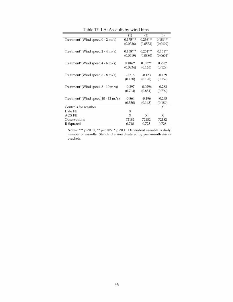
Table 17: LA: Assault, by wind bins(1) (2) (3)
Treatment*(Wind speed 0 - 2 m/s) 0.175*** 0.236*** 0.189***(0.0336) (0.0533) (0.0409)
Treatment*(Wind speed 2 - 4 m/s) 0.158*** 0.251*** 0.151**(0.0419) (0.0880) (0.0604)
Treatment*(Wind speed 4 - 6 m/s) 0.184** 0.377** 0.252*(0.0834) (0.165) (0.129)
Treatment*(Wind speed 6 - 8 m/s) -0.216 -0.123 -0.159(0.138) (0.198) (0.159)
Treatment*(Wind speed 8 - 10 m/s) -0.297 -0.0296 -0.282(0.764) (0.851) (0.794)
Treatment*(Wind speed 10 - 12 m/s) -0.864 -0.196 -0.265(0.550) (0.143) (0.189)
Controls for weather XDate FE XAQS FE X X XObservations 72182 72182 72182R-Squared 0.748 0.725 0.728
Notes: *** p<0.01, ** p<0.05, * p<0.1. Dependent variable is dailynumber of assaults. Standard errors clustered by year-month are inbrackets.
56

Table 18: LA: Assault, by season(1) (2) (3)
Treatment (West*Location dummy) -0.108* -0.128 -0.0120(0.0556) (0.110) (0.101)
Treatment*Spring 0.261** 0.393* 0.263(0.0793) (0.203) (0.179)
Treatment*Summer 0.339** 0.454** 0.203(0.0846) (0.210) (0.156)
Treatment*Autumn 0.296** 0.384* 0.180(0.0855) (0.211) (0.179)
Main Effects XControls for weather XDate FE XAQS FE X X XObservations 72182 72182 72182R-Squared 0.748 0.725 0.728
Notes: *** p<0.01, ** p<0.05, * p<0.1. Reference season in theinteraction is winter. Robust standard errors reported. Dependentvariable is daily number of assaults. Standard errors clustered byyear-month are in brackets.
Table 19: LA: Assault, by weekday/weekend(1) (2) (3)
Treatment (West*Location dummy) 0.210*** 0.582*** 0.520***(0.0488) (0.0753) (0.0553)
Treatment*Weekday -0.0672 -0.475*** -0.479***(0.0563) (0.0451) (0.0444)
Main Effects XControls for weather XDate FE XAQS FE X X XObservations 72182 72182 72182R-Squared 0.748 0.726 0.729
Notes: *** p<0.01, ** p<0.05, * p<0.1. Dependent variable is dailynumber of assaults. Standard errors clustered by year-month are inbrackets.
57

Table 20: Chicago: Downwind violent crime, by season(1) (2) (3) (4)
Treatment (downwind) 0.0953*** -0.0305 -0.0305 0.00225(0.0218) (0.0204) (0.0192) (0.0206)
Treatment*Spring -0.0521 0.0981*** 0.0981*** 0.0528*(0.0349) (0.0311) (0.0294) (0.0302)
Treatment*Summer -0.0252 0.0783** 0.0783** 0.0296(0.0369) (0.0321) (0.0304) (0.0318)
Treatment*Autumn -0.0261 0.0303 0.0303 -0.00344(0.0342) (0.0299) (0.0283) (0.0290)
Main Effects X XRoute*Side FE X X XRoute*Date FE X XRoute*Side Weather Interact. XObservations 41730 41730 41730 41730R-Squared 0.0216 0.290 0.678 0.680
Notes: *** p<0.01, ** p<0.05, * p<0.1. Reference season in the interactionis winter. Robust standard errors reported. The dependent variable is thenumber of crimes within one mile of one side of the interstate.
Table 21: Chicago: Downwind violent crime, by week-day/weekend
(1) (2) (3) (4)Treatment (downwind) 0.0839*** 0.0363 0.0363* 0.0378*
(0.0268) (0.0232) (0.0220) (0.0221)
Treatment*Weekday -0.0201 -0.0185 -0.0185 -0.0200(0.0309) (0.0265) (0.0251) (0.0250)
Main Effects X XRoute*Side FE X X XRoute*Date FE X XRoute*Side Weather Interact. XObservations 41730 41730 41730 41730R-Squared 0.00485 0.278 0.678 0.680
Notes: *** p<0.01, ** p<0.05, * p<0.1. Robust standard errors reported.The dependent variable is the number of crimes within one mile of oneside of the interstate.
58
Top Related