


Languages
Pages
Legal

Advancement and Analysis of a Gauss Pseudospectral
Transcription for Optimal Control Problemsby
Geoffrey Todd HuntingtonB. S. Aerospace Engineering, University of California, Los Angeles, 2001
S. M. Aerospace Engineering, Massachusetts Institute of Technology, 2003Submitted to the Department of Aeronautics and Astronautics
in partial fulfillment of the requirements for the degree ofDoctor of Philosophy
inAeronautics and Astronautics
at theMASSACHUSETTS INSTITUTE OF TECHNOLOGY
June 2007c© Geoffrey Todd Huntington, MMVII. All rights reserved.
The author hereby grants to MIT permission to reproduce and distribute
publicly paper and electronic copies of this thesis document in whole or inpart.
Author . . . . . . . . . . . . . . . . . . . . . . . . . . . . . . . . . . . . . . . . . . . . . . . . . . . . . . . . . . . . . . . . . . . .
Department of Aeronautics and AstronauticsMay 11, 2007
Certified by . . . . . . . . . . . . . . . . . . . . . . . . . . . . . . . . . . . . . . . . . . . . . . . . . . . . . . . . . . . . . . .
Jonathan P. How, Ph.D., ProfessorDepartment of Aeronautics and Astronautics, MIT
Thesis Committee Co-Chair
Certified by . . . . . . . . . . . . . . . . . . . . . . . . . . . . . . . . . . . . . . . . . . . . . . . . . . . . . . . . . . . . . . .Anil V. Rao, Ph. D., Assistant Professor
Dept. of Mechanical and Aerospace Engineering, University of Florida
Thesis Committee Co-ChairAccepted by . . . . . . . . . . . . . . . . . . . . . . . . . . . . . . . . . . . . . . . . . . . . . . . . . . . . . . . . . . . . . . .
Jaime Peraire, Ph.D., ProfessorDepartment of Aeronautics and Astronautics, MIT
Chair, Committee on Graduate Students

[This page intentionally left blank.]

Advancement and Analysis of a Gauss Pseudospectral
Transcription for Optimal Control Problems
by
Geoffrey Todd Huntington
Author . . . . . . . . . . . . . . . . . . . . . . . . . . . . . . . . . . . . . . . . . . . . . . . . . . . . . . . . . . . . . . . . . . . .
Department of Aeronautics and Astronautics
May 11, 2007
Certified by . . . . . . . . . . . . . . . . . . . . . . . . . . . . . . . . . . . . . . . . . . . . . . . . . . . . . . . . . . . . . . .
Jonathan P. How, Ph.D., ProfessorDepartment of Aeronautics and Astronautics, MIT
Thesis Committee Co-Chair
Certified by . . . . . . . . . . . . . . . . . . . . . . . . . . . . . . . . . . . . . . . . . . . . . . . . . . . . . . . . . . . . . . .
Anil V. Rao, Ph. D., Assistant ProfessorDept. of Mechanical and Aerospace Engineering, University of Florida
Thesis Committee Co-Chair
Certified by . . . . . . . . . . . . . . . . . . . . . . . . . . . . . . . . . . . . . . . . . . . . . . . . . . . . . . . . . . . . . . .David W. Miller, Ph.D., Professor
Department of Aeronautics and Astronautics, MITThesis Advisor
Certified by . . . . . . . . . . . . . . . . . . . . . . . . . . . . . . . . . . . . . . . . . . . . . . . . . . . . . . . . . . . . . . .
Raymond J. Sedwick, Ph.D., Principal Research ScientistDepartment of Aeronautics and Astronautics, MIT
Thesis Advisor
Certified by . . . . . . . . . . . . . . . . . . . . . . . . . . . . . . . . . . . . . . . . . . . . . . . . . . . . . . . . . . . . . . .Ronald J. Proulx, Ph.D., Principal Member of the Technical Staff
Charles Stark Draper Laboratory
Thesis Advisor

[This page intentionally left blank.]

Advancement and Analysis of a Gauss Pseudospectral
Transcription for Optimal Control Problems
by
Geoffrey Todd Huntington
Submitted to the Department of Aeronautics and Astronauticson May 11, 2007, in partial fulfillment of the
requirements for the degree ofDoctor of Philosophy
inAeronautics and Astronautics
Abstract
As optimal control problems become increasingly complex, innovative numerical methods areneeded to solve them. Direct transcription methods, and in particular, methods involvingorthogonal collocation have become quite popular in several field areas due to their highaccuracy in approximating non-analytic solutions with relatively few discretization points.Several of these methods, known as pseudospectral methods in the aerospace engineeringcommunity, have also established costate estimation procedures which can be used to verifythe optimality of the resulting solution. This work examines three of these pseudospectralmethods in detail, specifically the Legendre, Gauss, and Radau pseudospectral methods, inorder to assess their accuracy, efficiency, and applicability to optimal control problems ofvarying complexity. Emphasis is placed on improving the Gauss pseudospectral method,where advancements to the method include a revised pseudospectral transcription for prob-lems with path constraints and differential dynamic constraints, a new algorithm for thecomputation of the control at the boundaries, and an analysis of a local versus global imple-mentation of the method. The Gauss pseudospectral method is then applied to solve currentproblems in the area of tetrahedral spacecraft formation flying. These optimal control prob-lems involve multiple finite-burn maneuvers, nonlinear dynamics, and nonlinear inequalitypath constraints that depend on both the relative and inertial positions of all four space-craft. Contributions of this thesis include an improved numerical method for solving optimalcontrol problems, an analysis and numerical comparison of several other competitive directmethods, and a greater understanding of the relative motion of tetrahedral formation flight.
Thesis Committee Co-Chair: Jonathan P. How, Ph.D., ProfessorTitle: Department of Aeronautics and Astronautics, MIT
Thesis Committee Co-Chair: Anil V. Rao, Ph. D., Assistant ProfessorTitle: Dept. of Mechanical and Aerospace Engineering, University of Florida
5

[This page intentionally left blank.]

Acknowledgments
For my part I know nothing with any certainty, but the sight of the stars makes me dream...
- V. van Gogh
Looking back on my experience as a doctoral candidate, only now do I realize that a
Ph.D. is more about the journey than the end result. In that respect, I feel an even greater
sense of accomplishment and growth than I do for the results in this thesis. Part of this was
a result of my own maturation and increasing respect for past accomplishments in the field,
but it was mostly due to the fact that I had two excellent co-advisors. Prof. Anil Rao, your
tireless effort and attention to detail is inspiring and taught me that you should take nothing
for granted; to truly know a topic, you must fully understand even the smallest facets of
the problem. Prof. Jon How, your ability to cut straight to the root of a problem gave
me direction, especially when I needed it most. To the rest of my committee: Prof. Dave
Miller, Dr. Ray Sedwick, and Dr. Ron Proulx, your comments both in and out of committee
meetings were invaluable and helped me identify what the key research areas were.
In the course of my research, I read piles of papers and books, but there really was no
substitute for just picking up the phone and calling the author. To all the fellow academics
who helped me understand the vast amount of literature, I thank you. Specifically, I’d like
to thank Dr. John Betts, Prof. Larry Biegler, Juan Arrieta-Camacho, Prof. Qi Gong, Prof.
Wei Kang, Dr. Mark Milam, Jeremy Schwartz, Prof. William Hager, Prof. Claudio Canuto,
Prof. Phillip Gill, Prof. Gamal Elnagar, and Prof. Mohammad Kazemi. I’d especially like
to thank my old officemate, Dr. David Benson. I’ll never forget all the days of bouncing
both balls and ideas off each other!
A large part of what made my doctoral experience so enjoyable was the assurance of
funding, compliments of Draper Labs. So to George Schmidt and the rest of the education
department at Draper, thank you for sticking with me to the end! As for the Aerospace
Controls Lab at MIT, you made sharing a room with 20 people actually enjoyable, and for
that I thank you!
7
Lastly, I have to mention my incredible support network of friends and family. To the
IM sports crew, you were my stress relief. To all the taco nite attendees, your thirst for
margaritas and homemade taco shells kept me true to my ”work hard, play hard” motto.
To my ever-supportive family, thank you for offering whatever was needed all along the way.
When I make it to space, it will be because of you. And the best for last: to my lovely bride
Katie, the wait is over. I’m coming home.
This thesis was prepared at The Charles Stark Draper Laboratory, Inc., and was partially
funded by the NASA Goddard Spaceflight Center under Cooperative Agreement NAS5-
NCC5-730.
Publication of this thesis does not constitute approval by Draper or the sponsoring agency of
the findings or conclusions contained herein. It is published for the exchange and stimulation
of ideas.
Geoffrey Todd Huntington . . . . . . . . . . . . . . . . . . . . . . . . . . . . . . . . . . . . . . . . . . . . . . . . . . . . . . . . . . . . . . . .
8
ASSIGNMENT
Draper Laboratory Report Number T-1583
In consideration of the research opportunity and permission to prepare my thesis by and at
The Charles Stark Draper Laboratory, Inc., I hereby assign my copyright to The Charles
Stark Draper Laboratory, Inc., Cambridge, Massachusetts.
Author’s Signature Date
9

[This page intentionally left blank.]
Contents
1 Introduction 23
1.1 Motivation for Research . . . . . . . . . . . . . . . . . . . . . . . . . . . . . 27
1.1.1 Advancement of Numerical Methods for Optimal Control Problems . 27
1.1.2 Optimization of Formation Flying Maneuvers . . . . . . . . . . . . . 30
1.2 Contributions & Thesis Summary . . . . . . . . . . . . . . . . . . . . . . . . 32
2 Mathematical Background 35
2.1 Optimal Control . . . . . . . . . . . . . . . . . . . . . . . . . . . . . . . . . 35
2.1.1 Continuous Bolza Problem . . . . . . . . . . . . . . . . . . . . . . . . 35
2.1.2 Indirect Approach . . . . . . . . . . . . . . . . . . . . . . . . . . . . . 37
2.1.3 Direct Approach . . . . . . . . . . . . . . . . . . . . . . . . . . . . . 39
2.2 Numerical Approximation Methods . . . . . . . . . . . . . . . . . . . . . . . 42
2.2.1 Global Polynomial Approximations . . . . . . . . . . . . . . . . . . . 42
2.2.2 Quadrature Approximation . . . . . . . . . . . . . . . . . . . . . . . 44
2.2.3 Orthogonal Collocation . . . . . . . . . . . . . . . . . . . . . . . . . . 49
3 The Gauss Pseudospectral Method 51
3.1 Direct Transcription Formulation . . . . . . . . . . . . . . . . . . . . . . . . 51
3.1.1 Gauss Pseudospectral Discretization of Transformed Continuous Bolza
Problem . . . . . . . . . . . . . . . . . . . . . . . . . . . . . . . . . . 55
3.1.2 A Comment on the Final State: Xf . . . . . . . . . . . . . . . . . . . 56
3.1.3 Discontinuities & Phases . . . . . . . . . . . . . . . . . . . . . . . . . 58
3.2 Costate Approximation . . . . . . . . . . . . . . . . . . . . . . . . . . . . . . 59
11
3.2.1 KKT Conditions of the Transcribed NLP . . . . . . . . . . . . . . . . 62
3.2.2 Gauss Pseudospectral Discretization of the First-Order Necessary Con-
ditions . . . . . . . . . . . . . . . . . . . . . . . . . . . . . . . . . . . 69
3.2.3 Costate Mapping Theorem . . . . . . . . . . . . . . . . . . . . . . . . 71
3.3 Convergence . . . . . . . . . . . . . . . . . . . . . . . . . . . . . . . . . . . . 74
3.4 Summary . . . . . . . . . . . . . . . . . . . . . . . . . . . . . . . . . . . . . 76
4 Improving the Boundary Control 77
4.1 Algorithm for Computation of Boundary Controls . . . . . . . . . . . . . . . 78
4.2 Applications of Boundary Control Algorithm . . . . . . . . . . . . . . . . . . 80
4.2.1 Unconstrained Problem . . . . . . . . . . . . . . . . . . . . . . . . . . 81
4.2.2 Problem with a Path Constraint . . . . . . . . . . . . . . . . . . . . . 84
4.2.3 Launch Vehicle Ascent Problem . . . . . . . . . . . . . . . . . . . . . 86
4.3 Summary . . . . . . . . . . . . . . . . . . . . . . . . . . . . . . . . . . . . . 95
5 Local versus Global Orthogonal Collocation Methods 99
5.1 Local GPM Approach: Segments . . . . . . . . . . . . . . . . . . . . . . . . 100
5.2 Global and Local Applications of the GPM . . . . . . . . . . . . . . . . . . . 102
5.2.1 Modified Hicks-Ray Reactor Problem . . . . . . . . . . . . . . . . . . 102
5.2.2 Problem with Discontinuous Control . . . . . . . . . . . . . . . . . . 105
5.3 Summary . . . . . . . . . . . . . . . . . . . . . . . . . . . . . . . . . . . . . 111
6 Comparison between Three Pseudospectral Methods 115
6.1 Continuous Mayer Problem . . . . . . . . . . . . . . . . . . . . . . . . . . . 115
6.2 First-Order Necessary Conditions of Continuous Mayer Problem . . . . . . . 116
6.3 Descriptions of the Pseudospectral Methods . . . . . . . . . . . . . . . . . . 117
6.3.1 Legendre Pseudospectral Method (LPM) . . . . . . . . . . . . . . . . 118
6.3.2 Radau Pseudospectral Method (RPM) . . . . . . . . . . . . . . . . . 119
6.3.3 Gauss Pseudospectral Method (GPM) . . . . . . . . . . . . . . . . . 121
6.4 Costate Estimation . . . . . . . . . . . . . . . . . . . . . . . . . . . . . . . . 123
6.5 Comparison of Pseudospectral Methods . . . . . . . . . . . . . . . . . . . . . 128
12

6.5.1 Single State Example . . . . . . . . . . . . . . . . . . . . . . . . . . . 128
6.5.2 Two State Example . . . . . . . . . . . . . . . . . . . . . . . . . . . . 134
6.5.3 Orbit-Raising Problem . . . . . . . . . . . . . . . . . . . . . . . . . . 138
6.6 Rationale for Choosing a Method . . . . . . . . . . . . . . . . . . . . . . . . 141
6.7 Summary . . . . . . . . . . . . . . . . . . . . . . . . . . . . . . . . . . . . . 143
7 Tetrahedral Formation Flying 147
7.1 Overview of Spacecraft Formation Configuration Problem . . . . . . . . . . 147
7.2 Spacecraft Model and Equations of Motion . . . . . . . . . . . . . . . . . . . 149
7.2.1 Spacecraft Model . . . . . . . . . . . . . . . . . . . . . . . . . . . . . 149
7.2.2 Dynamic Model During Thrust Phases . . . . . . . . . . . . . . . . . 149
7.2.3 Dynamic Model for Coast Phases . . . . . . . . . . . . . . . . . . . . 150
7.2.4 Dynamic Model for Terminal Phase . . . . . . . . . . . . . . . . . . . 151
7.3 Constraints . . . . . . . . . . . . . . . . . . . . . . . . . . . . . . . . . . . . 151
7.3.1 Initial Conditions . . . . . . . . . . . . . . . . . . . . . . . . . . . . . 152
7.3.2 Interior Point Constraints . . . . . . . . . . . . . . . . . . . . . . . . 153
7.3.3 Path Constraints . . . . . . . . . . . . . . . . . . . . . . . . . . . . . 153
7.3.4 Terminal Constraints . . . . . . . . . . . . . . . . . . . . . . . . . . . 154
7.4 Spacecraft Orbit Insertion Optimal Control Problem . . . . . . . . . . . . . 156
7.5 Numerical Solution via Gauss Pseudospectral Method . . . . . . . . . . . . . 156
7.6 Results . . . . . . . . . . . . . . . . . . . . . . . . . . . . . . . . . . . . . . . 157
7.6.1 Two-Maneuver Solution . . . . . . . . . . . . . . . . . . . . . . . . . 157
7.6.2 Single-Maneuver Solution . . . . . . . . . . . . . . . . . . . . . . . . 164
7.6.3 Analysis of Optimality for the 1-Maneuver Problem . . . . . . . . . . 167
7.7 Overview of the Spacecraft Reconfiguration Problem . . . . . . . . . . . . . 167
7.8 Spacecraft Model and Equations of Motion . . . . . . . . . . . . . . . . . . . 170
7.8.1 Spacecraft Model . . . . . . . . . . . . . . . . . . . . . . . . . . . . . 170
7.8.2 Equations of Motion . . . . . . . . . . . . . . . . . . . . . . . . . . . 171
7.9 Constraints . . . . . . . . . . . . . . . . . . . . . . . . . . . . . . . . . . . . 171
7.9.1 Initial Conditions . . . . . . . . . . . . . . . . . . . . . . . . . . . . . 172
13

7.9.2 Interior Point Constraints . . . . . . . . . . . . . . . . . . . . . . . . 173
7.9.3 Trajectory Path Constraints during Thrust Phases . . . . . . . . . . 173
7.9.4 Constraints in the Region of Interest Phase . . . . . . . . . . . . . . . 173
7.10 Tetrahedral Reconfiguration Optimal Control Problem . . . . . . . . . . . . 176
7.11 Numerical Solution via Gauss Pseudospectral Method . . . . . . . . . . . . . 176
7.12 Results . . . . . . . . . . . . . . . . . . . . . . . . . . . . . . . . . . . . . . . 177
7.12.1 Minimum-Fuel Solution for Qmin = 2.7 . . . . . . . . . . . . . . . . . 177
7.12.2 Ensuring Future Satisfaction of Quality Factor Constraint . . . . . . 180
7.13 Summary . . . . . . . . . . . . . . . . . . . . . . . . . . . . . . . . . . . . . 186
8 Conclusions 191
8.1 Thesis Summary . . . . . . . . . . . . . . . . . . . . . . . . . . . . . . . . . 191
8.2 Future Work . . . . . . . . . . . . . . . . . . . . . . . . . . . . . . . . . . . . 192
14

List of Figures
2-1 Lagrange polynomial approximation to the function 1/(1 + 16x2) using 25
equidistant points on the interval [−1, 1]. . . . . . . . . . . . . . . . . . . . 44
2-2 Approximation accuracy of t9 for uniform and non-uniform spacing as the
number of support points is increased . . . . . . . . . . . . . . . . . . . . . 45
2-3 Approximation accuracy of et for uniform and non-uniform spacing as the
number of support points is increased . . . . . . . . . . . . . . . . . . . . . 45
2-4 Legendre-Gauss, Legendre-Gauss-Radau, and Legendre-Gauss-Lobatto collo-
cation points for K = 10 on the interval [−1, 1] . . . . . . . . . . . . . . . . 48
2-5 Accuracy of the quadrature approximation to t9 using LG, LGL, and LGR
points as the number of points increases . . . . . . . . . . . . . . . . . . . . 48
2-6 Accuracy of the quadrature approximation to et using LG, LGL, and LGR
points as the number of points increases . . . . . . . . . . . . . . . . . . . . 49
3-1 Flow diagram of the Gauss pseudospectral transcription (both direct and in-
direct approaches). . . . . . . . . . . . . . . . . . . . . . . . . . . . . . . . . 72
4-1 Solution for the unconstrained problem. . . . . . . . . . . . . . . . . . . . . 82
4-2 Error in the initial control as the number of nodes is increased for a spline
extrapolation, a Lagrange extrapolation, or by using Pontryagin for the un-
constrained problem. . . . . . . . . . . . . . . . . . . . . . . . . . . . . . . 83
4-3 Error in the final control as the number of nodes is increased for a spline
extrapolation, a Lagrange extrapolation, or by using Pontryagin for the un-
constrained problem. . . . . . . . . . . . . . . . . . . . . . . . . . . . . . . 83
15

4-4 Error in the propagated cost as the number of nodes is increased for a spline
extrapolation, a Lagrange extrapolation, or by using Pontryagin for the un-
constrained problem. . . . . . . . . . . . . . . . . . . . . . . . . . . . . . . 84
4-5 Solution for the path constrained problem. . . . . . . . . . . . . . . . . . . 85
4-6 Error in the equality path constraint at τ0 as the number of nodes is increased
for a spline extrapolation, a Lagrange extrapolation, or by using Pontryagin
in the path constrained problem. . . . . . . . . . . . . . . . . . . . . . . . . 86
4-7 Error in the equality path constraint at τf as the number of nodes is increased
for a spline extrapolation, a Lagrange extrapolation, or by using Pontryagin
in the path constrained problem. . . . . . . . . . . . . . . . . . . . . . . . . 87
4-8 Error in the initial control, u1(t0), as the number of nodes is increased for a
spline extrapolation, a Lagrange extrapolation, or by using Pontryagin in the
path constrained problem. . . . . . . . . . . . . . . . . . . . . . . . . . . . . 87
4-9 Error in the initial control, u2(t0), as the number of nodes is increased for a
spline extrapolation, a Lagrange extrapolation, or by using Pontryagin in the
path constrained problem. . . . . . . . . . . . . . . . . . . . . . . . . . . . . 88
4-10 Error in the final control, u1(tf), as the number of nodes is increased for a
spline extrapolation, a Lagrange extrapolation, or by using Pontryagin in the
path constrained problem. . . . . . . . . . . . . . . . . . . . . . . . . . . . . 89
4-11 Error in the final control, u2(tf), as the number of nodes is increased for a
spline extrapolation, a Lagrange extrapolation, or by using Pontryagin in the
path constrained problem. . . . . . . . . . . . . . . . . . . . . . . . . . . . . 90
4-12 Error in the propagated cost as the number of nodes is increased for a spline
extrapolation, a Lagrange extrapolation, or by using Pontryagin for the path
constrained problem. . . . . . . . . . . . . . . . . . . . . . . . . . . . . . . 91
4-13 Optimal altitude profile for the Delta III launch vehicle example. . . . . . . 94
4-14 Profile of the three components of the optimal control for the Delta III launch
vehicle example. . . . . . . . . . . . . . . . . . . . . . . . . . . . . . . . . . 95
16
4-15 The difference in spline-extrapolated control, |ui(tk)− − ui(tk)
+|, at all three
interior phase interfaces in the launch vehicle example. Some differences are
significantly greater than the optimality tolerance of 1e − 6. . . . . . . . . . 96
4-16 The difference in Pontryagin-extrapolated control, |ui(tk)− − ui(tk)
+|, at all
three interior phase interfaces in the launch vehicle example. Almost all dif-
ferences lie below the optimality tolerance of 1e − 6. . . . . . . . . . . . . . . 96
5-1 Distribution of nodes and collocation points for both the global and local
approaches (N = 20). . . . . . . . . . . . . . . . . . . . . . . . . . . . . . . 103
5-2 BVP solution to the Hicks-Ray reactor problem. . . . . . . . . . . . . . . . 106
5-3 Convergence of Hicks-Ray Problem via global approach as a function of the
number of nodes, N . . . . . . . . . . . . . . . . . . . . . . . . . . . . . . . . 107
5-4 Convergence of Hicks-Ray problem via local approach as a function of the
number of segments, S (5 nodes per segment). . . . . . . . . . . . . . . . . 108
5-5 Solution to double integrator problem for initial conditions of Eq. (5.18) using
global LG collocation with 40 nodes. . . . . . . . . . . . . . . . . . . . . . . 109
5-6 Solution to double integrator problem for initial conditions of Eq. (5.18) using
local LG collocation with 8 segments of 5 nodes each. . . . . . . . . . . . . 110
5-7 Error in state and costate for the double integrator problem using initial
conditions of Eq. (5.18) and global LG collocation with 40 nodes. . . . . . . 111
5-8 Error in state and costate for the double integrator problem using initial
conditions of Eq. (5.18) and local LG collocation with 8 segments of 5 nodes
each. . . . . . . . . . . . . . . . . . . . . . . . . . . . . . . . . . . . . . . . 112
5-9 Solution to the double integrator problem with the initial conditions of Eq. (5.19)
and semi-global LG collocation with two segments of 20 nodes each. . . . . 113
5-10 Solution to the double integrator problem with the initial conditions of Eq. (5.19)
and local LG collocation. . . . . . . . . . . . . . . . . . . . . . . . . . . . . 113
5-11 Error in state and costate for the double integrator problem using initial
conditions of Eq. (5.19) and semi-global LG collocation with two segments of
20 LG points each. . . . . . . . . . . . . . . . . . . . . . . . . . . . . . . . . 114
17

5-12 Error in state and costate for the double integrator problem using initial
conditions of Eq. (5.19) and local LG collocation. . . . . . . . . . . . . . . . 114
6-1 Exact solution for the single state example . . . . . . . . . . . . . . . . . . . 129
6-2 State error for the single state example. . . . . . . . . . . . . . . . . . . . . 130
6-3 Control error for the single state example. . . . . . . . . . . . . . . . . . . . 132
6-4 Error in the propagated state for the single state example. . . . . . . . . . . 133
6-5 Costate error for the single state example. . . . . . . . . . . . . . . . . . . . 134
6-6 LPM costate error for the single state example. . . . . . . . . . . . . . . . . 135
6-7 State convergence for the single state example . . . . . . . . . . . . . . . . . 136
6-8 Costate convergence for the single state example . . . . . . . . . . . . . . . 137
6-9 Improved LPM costate convergence via closure conditions for the single state
example. . . . . . . . . . . . . . . . . . . . . . . . . . . . . . . . . . . . . . 138
6-10 Convergence of the final control, u(tf), for the single state example. . . . . . 139
6-11 Exact solution for the two state example. . . . . . . . . . . . . . . . . . . . 140
6-12 State error for the two state example . . . . . . . . . . . . . . . . . . . . . . 141
6-13 Control error for the two state example. . . . . . . . . . . . . . . . . . . . . 142
6-14 Error in the propagated state for the two state example . . . . . . . . . . . 143
6-15 Costate error for the two state example . . . . . . . . . . . . . . . . . . . . 144
6-16 State convergence for the two state example . . . . . . . . . . . . . . . . . . 144
6-17 Costate convergence for the two state example . . . . . . . . . . . . . . . . 145
6-18 Error in state r(t) for the orbit raising problem . . . . . . . . . . . . . . . . 145
6-19 Error in the costate λr(t) for the orbit raising problem . . . . . . . . . . . . 146
6-20 Convergence of costate λr for the orbit raising problem . . . . . . . . . . . . 146
7-1 Schematic of trajectory event sequence for the orbit insertion problem . . . 148
7-2 Three-dimensional view of optimal terminal tetrahedron for two-maneuver
problem . . . . . . . . . . . . . . . . . . . . . . . . . . . . . . . . . . . . . . 158
7-3 Optimal terminal tetrahedron viewed along the orbital plane for the two-
maneuver problem . . . . . . . . . . . . . . . . . . . . . . . . . . . . . . . . 159
7-4 SC #4 control for the 2nd maneuver in the two-maneuver problem . . . . . . 159
18

7-5 Spacecraft burn durations relative to time of reference perigee passage, t −tperigee, for spacecraft i = 1, . . . , 4 during the first burn phase for the two-
maneuver problem . . . . . . . . . . . . . . . . . . . . . . . . . . . . . . . . 160
7-6 Optimal fuel consumption m(i)0 − m
(i)f of spacecraft i = 1, . . . , 4 for the two-
maneuver problem . . . . . . . . . . . . . . . . . . . . . . . . . . . . . . . . 161
7-7 Optimal terminal tetrahedron viewed from normal to the orbital plane for the
two-maneuver problem . . . . . . . . . . . . . . . . . . . . . . . . . . . . . . 162
7-8 Radial control for the two-maneuver problem . . . . . . . . . . . . . . . . . . 163
7-9 Transverse control for the two-maneuver problem . . . . . . . . . . . . . . . 163
7-10 Normal control for the two-maneuver problem . . . . . . . . . . . . . . . . . 164
7-11 Optimal terminal tetrahedron viewed along orbital plane for the single-maneuver
problem . . . . . . . . . . . . . . . . . . . . . . . . . . . . . . . . . . . . . . 165
7-12 Optimal terminal tetrahedron viewed from normal to the orbital plane for the
single-maneuver problem . . . . . . . . . . . . . . . . . . . . . . . . . . . . 166
7-13 Spacecraft burn durations relative to time of reference perigee passage, t −tperigee, for spacecraft i = 1, . . . , 4 during the burn phase for the single-
maneuver problem . . . . . . . . . . . . . . . . . . . . . . . . . . . . . . . . 166
7-14 Error in radial control for the single-maneuver problem . . . . . . . . . . . . 168
7-15 Error in transverse control for the single-maneuver problem . . . . . . . . . 169
7-16 Error in normal control for the single-maneuver problem . . . . . . . . . . . 170
7-17 Schematic of the event sequence for the reconfiguration problem . . . . . . . 171
7-18 Initial tetrahedral configuration . . . . . . . . . . . . . . . . . . . . . . . . . 172
7-19 Fuel expenditure of each spacecraft for Qmin = 2.7. . . . . . . . . . . . . . . 178
7-20 Projection of initial tetrahedron into ECI YZ-Plane for Qmin = 2.7 . . . . . . 178
7-21 Projection of terminal tetrahedron into ECI YZ-Plane for Qmin = 2.7 . . . . 179
7-22 Quality factor in region of interest for Qmin = 2.7 . . . . . . . . . . . . . . . 180
7-23 Average length, L, in region of interest for Qmin = 2.7 . . . . . . . . . . . . . 181
7-24 Quality factor, Qgm, as a function of average length, L, in region of interest
for Qmin = 2.7. Note: slope of Qgm attains a maximum when L attains a
minimum. . . . . . . . . . . . . . . . . . . . . . . . . . . . . . . . . . . . . . 181
19

7-25 Evolution of tetrahedral quality (Qgm) over three-week period beyond tf in
region of interest for Qmin = 2.7 . . . . . . . . . . . . . . . . . . . . . . . . . 183
7-26 Evolution of average length, L, over three-week period after tf in region of
interest for Qmin = 2.7 . . . . . . . . . . . . . . . . . . . . . . . . . . . . . . 183
7-27 Evolution of quality factor, Qgm, over three-week period after tf in region of
interest for Qmin = 2.8 . . . . . . . . . . . . . . . . . . . . . . . . . . . . . . 184
7-28 Fuel expenditure of each spacecraft for Qmin = 2.8 . . . . . . . . . . . . . . . 185
7-29 Comparison of projection of terminal tetrahedra into ECI XZ-Plane for Qmin =
2.7 and Qmin = 2.8 . . . . . . . . . . . . . . . . . . . . . . . . . . . . . . . . 185
20
List of Tables
4.1 Properties of the Delta III launch vehicle . . . . . . . . . . . . . . . . . . . . 89
4.2 Constants used in the Delta III launch vehicle problem . . . . . . . . . . . . 92
5.1 Computational expense for both the global and local approach in the Hicks-
Ray reactor problem . . . . . . . . . . . . . . . . . . . . . . . . . . . . . . . 105
6.1 Definitions of Lagrange interpolation polynomials used in this work . . . . . 123
6.2 CPU Times for each example and each method, in seconds . . . . . . . . . . 143
7.1 Maneuver durations for the two-maneuver problem . . . . . . . . . . . . . . 158
7.2 Spacecraft initial conditions . . . . . . . . . . . . . . . . . . . . . . . . . . . 172
7.3 Phase durations (in minutes) for Qmin = 2.7 . . . . . . . . . . . . . . . . . . 179
7.4 Phase durations (in minutes) for Qmin = 2.8 case . . . . . . . . . . . . . . . . 186
21

[This page intentionally left blank.]

Chapter 1
Introduction
Optimal control problems date back to the 17th century with Johann Bernoulli’s famous
brachystochrone problem.125 Greek for “shortest time”, Bernoulli posed this problem to
his contemporaries, which attempts to find the path along which an object moves between
two points in a vertical plane under its own weight in the shortest time. Several esteemed
mathematicians including Wilhelm Gottfried Leibniz, the Marquis de l’Hopital, Isaac Newton
and both Johann and Jakob Bernoulli submitted solutions to the brachystochrone problem,
marking the beginnings of optimal control theory.
With over 300 years of research in this area, many significant advancements have been
made. Highlights of these advancements include the creation of calculus of variations, first
elaborated by Euler in 1733 in the Elementa Calculi Variatonum32 from which it got its
name. Also, in the 1950’s, Richard Bellman pioneered work in dynamic programming73
which led to sufficient conditions for optimality using the Hamilton-Jacobi-Bellman equation.
Lev Pontryagin’s development of the maximum (minimum) principle82 in 1962 provided a
method to determine the optimal control for constrained problems, often resulting in “bang-
bang” solutions. The availability of commercial computers in the 1950’s fundamentally
transformed the field by enabling efficient numerical solutions.21 Present-day numerical
methods for solving optimal control problems are plentiful and vary greatly in their approach
and complexity. These methods discretize the continuous-time problem in some fashion and
solve the resulting approximate, finite-dimensional problem to a specified tolerance.
Numerical methods for solving optimal control problems fall into two general categories:
23

indirect methods and direct methods. In an indirect method, first-order necessary conditions
for optimality are derived from the optimal control problem via the calculus of variations73
and Pontryagin’s minimum principle.82 These necessary conditions form a Hamiltonian
boundary-value problem (HBVP), which is then solved numerically for extremal trajecto-
ries.3 The optimal solution is then found by choosing the extremal trajectory with the lowest
cost. The primary advantages of indirect methods are a high accuracy in the solution and
the assurance that the solution satisfies the first-order optimality conditions. However, in-
direct methods have several disadvantages. First, the HBVP must be derived analytically,
which can often be non-trivial. Second, because indirect methods typically have small radii
of convergence, an extremely good initial guess of the unknown boundary conditions is gen-
erally required. Furthermore, many indirect methods require an accurate initial guess of the
costate, which is often non-intuitive and difficult to obtain. Finally for problems with path
constraints, it is necessary to have a priori knowledge of the constrained and unconstrained
arcs or switching structure. BNDSCO80 is a commercial program for solving multipoint
boundary value problems that implements an indirect multiple shooting algorithm.
In a direct method, the continuous-time optimal control problem is transcribed directly to
a nonlinear programming problem (NLP) without formulating an alternate set of optimality
conditions. The resulting NLP can be solved numerically by well developed algorithms,10,45
which attempt to satisfy a set of conditions (called Karush-Kuhn-Tucker (KKT) conditions)
associated with the NLP. Direct methods have the advantage that the first-order necessary
conditions do not need to be derived. Furthermore, they have much larger radii of con-
vergence than indirect methods and thus, do not require as good an initial guess, and do
not require an initial guess for the costate. Lastly, the switching structure does not need
to be known a priori. However, many direct methods have the disadvantage of providing
either an inaccurate costate or providing no costate information whatsoever, meaning it
is uncertain whether the optimal solution to the NLP is truly an optimal solution to the
original optimal control problem. Well-known software packages employing direct meth-
ods include Optimal Trajectories by Implicit Simulation (OTIS),119 Sparse Optimal Control
Software (SOCS),11 Graphical Environment for Simulation and Optimization (GESOP),122
Direct Collocation (DIRCOL),121 Nonlinear Trajectory Generation (NTG),78,79 and Direct
24

and Indirect Dynamic Optimization (DIDO).95
The category of direct methods is quite broad and encompasses some very different tech-
niques.64 In particular, the choice of what quantities to discretize and how to approximate
the continuous-time dynamics varies widely amongst the different direct methods. Two
of the more common types of direct methods are control parameterization and state and
control parameterization115 techniques. In a control parameterization method,16,102, 109, 130
the control alone is approximated and the differential equations are solved via numerical
integration. Examples of control parameterization include shooting methods and multiple
shooting methods. In state and control parameterization methods,14,37, 56, 57, 81, 107 the state
is discretized within the NLP as well as the control, and the continuous-time differential
equations are converted into algebraic constraints. These constraints are then imposed in
the NLP formulation, which avoid the sensitivity issues of direct shooting methods at the
expense of a larger NLP.
In recent years, considerable attention has been brought to a class of state and control
parameterization methods called pseudospectral23,33, 43 or orthogonal collocation26,116 meth-
ods. In a pseudospectral method, a finite basis of global interpolating polynomials is used
to approximate the state and control at a set of discretization points. The time derivative
of the state in the dynamic equations is approximated by the derivative of the interpo-
lating polynomial and is then constrained to be equal to the vector field of the dynamic
equations at a set of collocation points. While any set of unique collocation points can be
chosen, generally speaking an orthogonal collocation is chosen, i.e., the collocation points are
chosen to be the roots of an orthogonal polynomial (or linear combinations of such polyno-
mials and their derivatives). Because pseudospectral methods are generally implemented via
orthogonal collocation, the terms pseudospectral and orthogonal collocation are essentially
interchangeable (thus researchers in one field use the term pseudospectral43 while others use
the term orthogonal collocation116). One advantage to pseudospectral methods is that for
smooth problems, pseudospectral methods typically have faster convergence rates than other
methods, exhibiting so called “spectral accuracy”.112 For non-smooth problems or problems
where modeling changes are desired, the optimal control problem can be divided into phases
and orthogonal collocation can be applied globally within each phase. A vast amount of
25

work has been done on using pseudospectral methods to solve non-smooth optimal control
problems (see Refs. 27, 34, 38, 85, 92, 95).
Pseudospectral methods in optimal control arose from spectral methods which were tra-
ditionally used to solve fluid dynamics problems.23,43 Meanwhile, seminal work in orthogonal
collocation methods for optimal control problems date back to 1979 with the work of Ref. 87
and some of the first work using orthogonal collocation methods in engineering can be found
in the chemical engineering literature.27 More recent work in chemical and aerospace engi-
neering have used collocation at the Legendre-Gauss-Radau (LGR) points,41,71, 72 which is
termed the Radau pseudospectral method (RPM) in this thesis. Within the aerospace en-
gineering community, several well-known pseudospectral methods have been developed for
solving optimal control problems such as the Chebyshev pseudospectral method (CPM),117,118
the Legendre pseudospectral method (LPM),33 and the Gauss pseudospectral method (GPM).8
The CPM uses Chebyshev polynomials to approximate the state and control, and performs
orthogonal collocation at the Chebyshev-Gauss-Lobatto (CGL) points. An enhancement to
the Chebyshev pseudospectral method that uses a Clenshaw-Curtis quadrature was devel-
oped in Ref. 40. The LPM uses Lagrange polynomials for the approximations, and Legendre-
Gauss-Lobatto (LGL) points for the orthogonal collocation. A costate estimation procedure
for the Legendre pseudospectral method was developed by in Ref. 39 and recently updated
in Ref. 49. Recent work by Williams shows several variants of the standard LPM. The Jacobi
pseudospectral method126 is a more general pseudospectral approach that uses Jacobi poly-
nomials to find the collocation points, of which Legendre polynomials are a subset. Another
variant, called the Hermite-LGL method,128 uses piecewise cubic polynomials rather than La-
grange polynomials, and collocates at a subset of the LGL points. These new methods have
not yet become mainstream optimization techniques because of their novelty, but the new
software tool DIRECT127 could expedite this process. Lastly, in the Gauss pseudospectral
method, the state is approximated using a basis of Lagrange polynomials similar to the LPM,
and the optimal control problem is orthogonally collocated at the interior Legendre-Gauss
(LG) points. Much of the analysis done in this thesis centers on pseudospectral methods
and their accuracy and efficiency in numerically solving optimal control problems.
26

1.1 Motivation for Research
The research presented in this thesis is motivated by fundamental questions in two different
areas.
1.1.1 Advancement of Numerical Methods for Optimal Control
Problems
The Gauss pseudospectral method in its current form is one of the newest numerical ap-
proaches in the literature today,8 although it bears resemblance to work done in 1979.87 The
current method was originally developed for problems with integral dynamic equations, and
was then adapted to accommodate differential dynamic equations. The critical contribution
by Benson, which distinguishes the GPM among the other pseudospectral methods, was to
show that for an optimal control problem with either integral or differential dynamics, the
Karush-Kuhn-Tucker (KKT) conditions of the NLP are exactly equivalent to the discretized
form of the first-order optimality conditions of the HBVP. Hence, a solution to the NLP also
satisfies the optimality conditions traditionally used in indirect methods, thereby eliminating
one of the primary disadvantages of direct methods. Benson also showed that this equiv-
alence for the integral formulation existed in the presence of path constraints, but did not
explicitly show equivalence for problems with both path constraints and the more common
differential dynamic constraints. Therefore the first motivation for this thesis is to complete
the equivalence proof for the general formulation of the optimal control problem involving
both differential dynamic constraints and path constraints.
Costate Mapping using GPM
When analyzing the solution to optimal control problems, it is desirable for the solution
to include not only state and control approximations, but a costate approximation as well.
The ability to obtain accurate costate estimates is useful for verifying the optimality of
solutions, determining the sensitivity of the state with respect to cost, and performing mesh
refinement.14 Indirect methods naturally include the costate in their problem formulation, so
any indirect solution contains a costate estimate. However, direct methods do not explicitly
27
approximate the costate since the HBVP equations are not formulated. Despite this, a
costate estimate can be determined for many direct methods in several ways. Some of
these estimates are based on solving an approximation to the costate dynamics in post-
processing.58,76 Other estimates are based on relationships between the KKT multipliers of
the NLP and the continuous costate found by a sensitivity analysis,103 or relating the KKT
conditions of the NLP to the continuous costate dynamics.55,107 Or, for some pseudospectral
methods, the KKT multipliers can be algebraically mapped to the discrete costate via a
simple computation. Costate mapping procedures have been documented in Ref. 71 for
the RPM, Refs. 39, 49 for the LPM, and Ref. 8 for the GPM. Although an exact mapping
between the KKT multipliers and the discrete costate has not been proven for the RPM and
LPM, research has been done on these pseudospectral methods that discusses the (rapid)
convergence rates of the NLP solution to the solution of the continuous-time optimality
conditions.48,49, 71 Benson developed a costate mapping procedure for the GPM and proved it
was an exact map due to the equivalence between the KKT conditions and HBVP optimality
conditions. The aforementioned equivalence in the GPM brings about a certain mathematical
elegance that can possibly contain some undiscovered properties. Another motivation for
this research is to simply explore what additional benefits can be gleaned from the costate
mapping.
Analysis and Comparison of Various Pseudospectral Methods
With so many different approaches to solve optimal control problems, it is clear that the
academic community is fragmented on which approach may be the best for a general problem.
And it is likely that no one method works the best on all problems. However, very few
papers have been published that compare the performance of various methods. Survey
papers, such as Ref. 12, stop short of providing comparisons between various methods.
Numerical comparisons between methods are often difficult to perform fairly because many
direct methods are integrated with a specific NLP solver, thereby making it difficult to
distinguish between differences between the methods and differences due to the NLP solvers.
However, some research has been done that compares direct methods. Ref. 81 is primarily
focused on presenting enhanced mesh refinement and scaling strategies, but contains a brief
28

comparison of the accuracy of direct implicit integration schemes (like Hermite-Simpson
integration) and pseudospectral methods. Williams created the software tool DIRECT in
order to more effectively compare various trajectory optimization algorithms. The results
of a thorough comparison involving 21 test problems of several different direct methods
is presented in Ref. 127. Ref. 42 presents a comparison between several pseudospectral
approaches, but uses unorthodox variants of pseudospectral methods that are inconsistent
with a large majority of the literature. Based on this very limited body of research, there
exists a greater need to examine the accuracy and efficiency of these direct methods from a
numerical and theoretical standpoint.
Analysis and Comparison of Local versus Global Orthogonal Collocation Meth-
ods
Interestingly, when the Gauss pseudospectral method was first introduced to the academic
community, it received quite a bit of resistance and skepticism. Critics noted that historically,
local methods, i.e., those that approximate the dynamics locally using piecewise polynomials,
have been prosperous due to their property of local support,14 which bounds the maximum
error that can be generated locally along the trajectory. Consequently one can determine the
maximum error between the exact optimal solution and the computed solution for the entire
trajectory. While local methods have a long history in solving optimal control problems,
recent research in pseudospectral methods suggests that local collocation may neither be the
most accurate nor the most computationally efficient approach.8,48, 66, 68, 89 Instead, recent
work has shown great success in the application of global collocation (i.e., collocation using
a global polynomial across the entire time interval as the basis for approximation). By
using appropriate discretization points and interpolating polynomials, one can also bound
the maximum error generated by the global polynomial approximation, shown in Chapter
2. In fact, Ref. 81 specifically compares global pseudospectral methods to other local direct
collocation methods, and also experiments with the order of the local collocation methods
(i.e., the number of collocation points per segment) and its effect on the solution accuracy.
In light of the recent results that promote global orthogonal collocation and the long history
of the use local collocation, it is important to gain a better understanding as to how these
29

two different philosophies work in practice.
Computation of the Boundary Control Using the Gauss Pseudospectral Method
Other critics have highlighted the fact that since the Gauss pseudospectral method per-
forms collocation at the interior LG points, there is no explicit value for the control at the
boundary points. Consequently, the value for the boundary control can be quite arbitrary.
Moreover, traditional extrapolation techniques (such as spline extrapolation14 or Lagrange
extrapolation71) may violate control path constraints and certainly will be sub-optimal. Fur-
ther motivation for this research lies in the need to improve the accuracy of the boundary
control for the Gauss pseudospectral method.
1.1.2 Optimization of Formation Flying Maneuvers
Spacecraft formation flying is defined as a set of more than one spacecraft whose states are
coupled through a common control law.101 Formation flying has been identified as an enabling
technology for many future space missions.100 In particular, space missions using multiple
spacecraft, as compared with using a single spacecraft, allow simultaneous measurements to
be taken at specific relative locations, thereby improving science return. An important aspect
that is critical to the successful implementation of formation flying missions is trajectory
design (also called path planning or guidance100). An excellent survey of methods used
to design formation flying trajectories can be found in Ref. 100, which also provides an
extensive list of references on formation flying guidance. Formation flying trajectory design
has two main categories: stationkeeping, i.e., to maintain a relative spacecraft formation
for a specified portion of the trajectory and reconfiguration, i.e., to maneuver a spacecraft
formation from one configuration (involving the formation geometry, relative motion, and/or
orientation) to a second configuration.
A particular class of Earth-orbit formations that have been studied extensively are those
involving four spacecraft.17,25, 47, 53, 62, 66, 67 Four-spacecraft formations are desirable because
they use relatively few spacecraft yet are still capable of taking measurements in three-
dimensions at relatively large inter-spacecraft distances (e.g., a spacing of several kilome-
30

ters). However, because of complex mission constraints, it is often difficult to determine
feasible trajectories and controls. Because of the already difficult task of determining feasi-
ble solutions, it is even more of a challenge to determine solutions that minimize a specified
performance metric (e.g., trajectories that minimize fuel). Fuel-optimal solutions (if one can
be found) are often non-intuitive, but are very worthwhile as they can lead to significant fuel
savings which can result in a longer mission duration or increased payload capacity.
Several papers have attempted to solve tetrahedral trajectory optimization problems
similar to the ones considered in this research. Ref. 75 uses a two-step approach that begins
with genetic algorithms (a global heuristic optimization method) and afterwards refines the
problem using Lawden’s primer vector theory.5 Ref. 54 also uses a two-step approach, but
combines a direct SQP method with a genetic algorithm. Ref. 113 employs a three-step
approach that uses simulated annealing (another global heuristic method) as its initial step.
In each of these previous works, the problem is separated into steps where, in general, one
step optimizes the orbital transfer portion of the trajectory and the other step optimizes the
relative position constraints in a sequential but separate optimization procedure that uses
the trajectory from the first step. While dividing the problem into parts and optimizing each
part separately makes the problem more tractable, it also reduces the solution search space.
In this work the entire problem is formulated as a single unified numerical optimization
procedure. Other papers use a single numerical optimization procedure, but necessitate
significant simplifying assumptions on either the dynamic model111 or the search space60 in
order to make the problem more manageable. Lastly, Refs. 18, 19 use linearized dynamics,
but incorporate them into an MPC format, exhibiting a capability for real-time optimization
of formation flying maneuvers.
The formation flying problems posed in this thesis are based on the proposed NASA
Multi-scale Magnetospheric (MMS) Mission, which will attempt to make fundamental ad-
vancements in the understanding of the Earths magnetosphere and its dynamic interaction
with solar wind by measuring magnetic and electric fields.62,63 The mission intends to have
a four-spacecraft formation that forms a tetrahedral geometry when taking science data.
Very little is known about the characteristics of the fuel-optimal maneuvers for this type
of mission, so this research is primarily interested in gaining a better perspective on the
31
location, number, and duration of maneuvers needed to optimally reconfigure the spacecraft
between different configurations while simultaneously satisfying certain nonlinear geometric
path constraints along some region of the orbit.
1.2 Contributions & Thesis Summary
This section briefly describes the contents of the chapters in this thesis, and specifically
highlights the significant contributions.
In order to better understand the theoretical contributions in this thesis, there are several
mathematical concepts that are worth describing in detail within the thesis. Chapter 2
not only presents this material in a concise manner, but also discusses the rationale and
advantages for using these mathematical constructs.
Chapter 3 presents the Gauss pseudospectral method in its most current form. This
has been slightly modified from the original formulation in Ref. 6 in order to simplify the
notation, and provide a more complete NLP solution, which includes both path constraints
and differential dynamics in the optimal control problem formulation. Next, the equivalence
between the KKT conditions and the HBVP first-order optimality conditions is proved for
this new formulation, and a corresponding costate mapping theorem is derived. Lastly, this
chapter provides a discussion on past and present attempts to prove the convergence of
the NLP solution towards the exact optimal solution as the number of discretization points
increases towards infinity.
Chapter 4 directly addresses some of the critics’ concerns that the Gauss pseudospectral
method is an ill-conceieved approach because it does not provide an explicit value for the
boundary control from the NLP. Traditional methods involving extrapolation are presented,
along with a new procedure for computing a highly accurate boundary control from the NLP
solution. These approaches are compared on several example problems including a complex
multi-stage launch vehicle problem.
Chapter 5 directly addresses some of the other critics’ concerns regarding local versus
global approaches to optimal control problems, as mentioned earlier in this chapter. This
chapter outlines the rationale and procedure for each approach and references the current
32

work in both approaches. The comparison is conducted using the Gauss pseudospectral
method, which is implemented in both a local and global fashion. The comparison is made
on two example problems that have characteristics that might suggest the use of a local
approach. The computational accuracy and efficiency are analyzed for both examples.
In Chapter 6, a comparison is made between three commonly used pseudospectral meth-
ods: the Legendre, Radau, and Gauss pseudospectral methods. In order to provide a fair
comparison, in this study the NLP solver SNOPT45 is used for each of the discretizations.
Furthermore, all three methods are implemented using the same version of MATLAB R© and
the initial guesses provided for all examples are identical. Using this equivalent setup for all
three methods, the goal of the study is to assess the similarities and differences in the accu-
racy and and computational performance between the three methods. Three examples are
used to make the comparison. The first two examples are designed to be sufficiently simple
so that the key features of each method can be identified and analyzed. The third example,
a commonly used problem in aerospace engineering, is designed to provide an assessment as
to how the three methods compare on a more realistic problem. A great deal of the emphasis
of this study is to understand when one method may perform better than another method
and to identify why such an improved performance is attained in such circumstances.
Chapter 7 considers several spacecraft reconfiguration problems. The first problem is
what’s typically known as an orbit insertion problem or initialization problem,75 meaning the
four spacecraft must optimally maneuver from an initial parking orbit to the desired mission
orbit and satisfy certain formation configuration constraints upon reaching the mission orbit.
As formation flying missions continue throughout their mission lifetime, disturbances will
cause the spacecraft to naturally drift apart from one another, thus creating a “degraded”
formation. The second scenario addresses this issue by examining the problem of optimally
reconfiguring a four-spacecraft formation from an initial degraded formation to a formation
that satisfies a set of mission constraints along a region of the orbit (representing the scientific
area of interest for the mission). Both the orbit insertion problem and the reconfiguration
problem are posed as optimal control problems. These complex optimal control problems
are highly nonlinear and have no analytic solutions. Consequently, they are transcribed into
an NLP using the Gauss pseudospectral method. A greater understanding for the relative
33

motion of spacecraft formations, the location of minimum-fuel maneuvers, and minimum-fuel
tetrahedral geometries is developed in this chapter.
Finally, Chapter 8 summarizes the significant contributions of this thesis and suggests
potential future research directions.
34
Chapter 2
Mathematical Background
This chapter introduces several of the theoretical and mathematical concepts used in this
thesis. Many of the advancements in this thesis are founded on optimal control theory,
and a significant portion of this chapter explains the fundamentals of optimal control. This
work also largely relies on numerical approximations, and several approaches to function
approximation and quadrature approximation are described in detail.
2.1 Optimal Control
As explained concisely by Kirk in Ref. 73, the objective of an optimal control problem is to
determine the control signals that will cause a process to satisfy the physical, geometric, or
design constraints and at the same time minimize (or maximize) some performance criterion.
This section describes the optimal control problem in a more mathematical framework, and
discusses common approaches to solving optimal problems.
2.1.1 Continuous Bolza Problem
Consider the following general optimal control problem. Determine the control, u(t) ∈ Rm,
that minimizes the Bolza cost functional
J = Φ(x(t0), t0,x(tf ), tf) +
∫ tf
t0
g(x(t),u(t), t)dt (2.1)
35

involving the state, x(t) ∈ Rn, the initial time, t0, and (free or fixed) final time, tf , subject
to the dynamic constraint
x(t) = f(x(t),u(t), t), t ∈ [t0, tf ] (2.2)
the boundary condition
φ(x(t0), t0,x(tf), tf ) = 0 (2.3)
and inequality path constraint
C(x(t),u(t), t) ≤ 0, t ∈ [t0, tf ] (2.4)
In Eqs. (2.1)-(2.4), the functions Φ, g, f, φ, and C are defined as follows:
Φ : Rn × R × R
n × R → R
g : Rn × R
m × R → R
f : Rn × R
m × R → Rn
φ : Rn × R × R
n × R → Rq
C : Rn × R
m × R → Rc
(2.5)
The problem of Eqs. (2.1)-(2.4) is referred to as the continuous Bolza problem.
The Bolza problem is defined on the time interval t ∈ [t0, tf ]. Certain numerical tech-
niques (like pseudospectral methods) require a fixed time interval, such as [−1, 1]. The
independent variable can be mapped to the general interval τ ∈ [−1, 1] via the affine trans-
formation
τ =2t
tf − t0− tf + t0
tf − t0(2.6)
Note that this mapping is still valid with free initial and final times. Using Eq. (2.6), the
Bolza problem can be redefined as follows. Minimize the cost functional
J = Φ(x(τ0), t0,x(τf ), tf) +tf − t0
2
∫ τf
τ0
g(x(τ),u(τ), τ ; t0, tf)dτ (2.7)
36

subject to the constraints
dx
dτ=
tf − t02
f(x(τ),u(τ), τ ; t0, tf) (2.8)
φ(x(τ0), t0,x(τf ), tf) = 0 (2.9)
C(x(τ),u(τ), τ ; t0, tf) ≤ 0 (2.10)
The problem of Eqs. (2.7)–(2.10) is referred to as the transformed continuous Bolza problem.
2.1.2 Indirect Approach
The transformed Bolza problem of Eqs. (2.7)–(2.10) historically has been solved using a
branch of mathematics called calculus of variations to obtain a set of first-order necessary
conditions for optimality.20,73, 74 A solution to the optimality conditions is called an extremal
solution, and second-order conditions can be checked to ensure that the extremal solution is
a minimum. The fundamental theorem of the calculus of variations is73
If x∗ is an extremal, the variation of the cost, J , must vanish on x∗; that is,
δJ(x∗, δx) = 0, ∀ admissible δx (2.11)
The first-order necessary conditions are found by taking the first-order variation of the
augmented cost functional, which is created by adjoining the constraints to the cost functional
via adjoint variables (i.e., costate, λ(τ) ∈ ℜn) and Lagrange multipliers, ν ∈ ℜq and µ(τ) ∈ℜc as
Ja = Φ(x(τ0), t0,x(τf ), tf) − νT φ(x(τ0), t0,x(τf ), tf) +tf − t0
2
∫ 1
−1
[
g(x(τ),u(τ), τ ; t0, tf)
−λT (t)
(
dx
dτ− f(x(τ),u(τ), τ ; t0, tf)
)
− µT (τ)C(x(τ),u(τ), τ ; t0, tf)
]
dτ
(2.12)
The variation with respect to each free variable is then set to zero, as in Eq. (2.11) and
results in a set of first-order necessary conditions for optimality. This approach is commonly
called “indirect”, as it indirectly solves the original problem by formulating and solving
37

this alternate set of optimality conditions. Often, the first-order optimality conditions are
simplified by defining an augmented Hamiltonian functional, H, as
H(x, λ, µ,u, τ ; t0, tf) = g(x,u, τ ; t0, tf) + λT f(x,u, τ ; t0, tf) − µTC(x,u, τ ; t0, tf) (2.13)
which includes the costate, λ(τ) ∈ Rn, and Lagrange multiplier function associated with
the path constraint, µ(τ) ∈ Rc. For brevity, the explicit dependence on time, τ , for the
state, control, costate, and Lagrange multiplier has been dropped. The first-order optimality
conditions are also referred to as the Hamiltonian boundary value problem (HBVP):
dx
dτ
T
=tf − t0
2fT (x,u, τ ; t0, tf ) =
tf − t02
∂H∂λ
dλ
dτ
T
=tf − t0
2
(
−∂g
∂x− λT ∂f
∂x+ µT ∂C
∂x
)
= −tf − t02
∂H∂x
0T =∂g
∂u+ λT ∂f
∂u− µT ∂C
∂u=
∂H∂u
φ(x(τ0), t0,x(τf ), tf) = 0
λ(τ0)T = − ∂Φ
∂x(τ0)+ νT ∂φ
∂x(τ0)
λ(τf )T =
∂Φ
∂x(τf )− νT ∂φ
∂x(τf )
H(t0) =∂Φ
∂t0− νT ∂φ
∂t0
H(tf) = −∂Φ
∂tf+ νT ∂φ
∂tf
µj(τ) = 0 , when Cj(x,u, τ ; t0, tf ) < 0 , j = 1, . . . , c
µj(τ) ≤ 0 , when Cj(x,u, τ ; t0, tf) = 0 , j = 1, . . . , c
(2.14)
where ν ∈ Rq is Lagrange multiplier associated with the boundary condition φ. For some
problems, the control cannot be uniquely determined, either implicitly or explicitly, from
these optimality conditions. In such cases, the weak form of Pontryagin’s minimum principle
can be used which solves for the permissible control that globallly minimizes the augmented
Hamiltonian in Eq. (2.13). If U is the set of permissible controls, then Pontryagin’s minimum
38

principle73 states that the optimal control, u∗ ∈ U , satisfies the following:
H(x∗,u∗, λ∗, µ∗, τ ; t0, tf ) ≤ H(x∗,u, λ∗, µ∗, τ ; t0, tf), ∀u ∈ U , τ ∈ [−1, 1] (2.15)
Note that the equations described in this section constitute a set of necessary conditions for
optimality, but they are not sufficient conditions. A second order sufficiency check can be
implemented to confirm that the extremal solution is the desired minimum or maximum.
The necessary conditions for optimality involve not only the state and control, but the
costate as well, emphasizing the importance of the costate in an extremal solution. Without
a costate, one cannot check the necessary and sufficient conditions to ensure that an optimal
solution has been found. Furthermore, the costate provides information regarding the sensi-
tivity of the minimum cost with respect to the corresponding extremal state.73 Specifically,
let δJ∗(x∗(τ), τ, δx(τ)) denote the first-order approximation to the change in the minimum
cost that results when the state at time τ deviates from x∗(τ) by an amount δx(τ). Then
δJ∗(x∗(τ), τ, δx(τ)) = λ∗T (τ)δx(τ) (2.16)
Thus the sensitivities represented by the costate are often used to redesign the original
optimal control problem if the constraints on the problem are flexible.
2.1.3 Direct Approach
The optimality conditions of Eq. (2.14) are often not trivial to formulate. Furthermore,
numerical methods that solve these equations generally require an accurate guess for the
costate, which is often non-intuitive. For these reasons and others suggested in Chapter 1,
direct methods have become a very popular alternative to indirect methods in recent years.
Rather than formulate a set of optimality conditions, direct methods transcribe or convert the
infinite-dimensional optimal control problem into a finite-dimensional optimization problem
with algebraic constraints, also known as a nonlinear program (NLP).
As explained by Betts in Ref. 14, a direct transcription method has three fundamental
steps:
39
1. convert the dynamic system into a problem with a finite set of variables and algebraic
constraints, then
2. solve the finite-dimensional problem using a parameter optimization method, then
3. assess the accuracy of the finite-dimensional approximation and if necessary repeat the
transcription and optimization steps.
Some direct methods discretize only the control, and propagate the dynamics across
the interval using the control approximation. Any additional constraints are checked to
ensure feasibility, and along with the cost, help determine the search direction for NLP.
These methods are called “shooting methods”, named after the early application of aiming a
cannon such that the cannonball hit its target.14 Other methods discretize both the state and
control, and are hence called state and control parameterization methods. These methods
are further subdivided into local and global methods. Local methods break the dynamics
into subintervals at the points t0 ≤ t1, . . . , ti, . . . , tN ≤ tf , and attempt to find the state and
control that satisfy
xi+1 = xi +
∫ ti+1
ti
f(x,u, t)dt (2.17)
where the integral is then replaced with some quadrature approximation:
∫ ti+1
ti
f(x,u, t)dt ≈ hi
K∑
j=1
βjf(xj ,uj, τj), ti ≤ τj ≤ ti+1 (2.18)
Euler, Runge-Kutta, Trapezoidal, and Hermite-Simpson methods are all popular one-step
local methods. Adams schemes, such as Adams-Moulton and Adams-Bashforth schemes are
multi-step methods, meaning their integration steps involve more than just xi and xi+1.
Multi-step methods have the general form:
xi+k =
k−1∑
j=0
αjxi+j + h
k∑
j=0
βjfi+j (2.19)
where αj and βj are known constants. Global schemes go even further than multi-step
schemes in that they span the entire problem interval. Global, or pseudospectral methods
40

are extensively used in the numerical solution to partial differential equations, with the most
common types of methods being Galerkin, Tau, and Collocation methods.23 Pseudospectral
methods, as explained by Fornberg in Ref. 43, approximate the solution, x(t), by a finite
sum, X(t) =∑M
k=1 akφk(t). The two main questions that arise are then:
1. from which function class should φk(t), k = 1, . . . , M be chosen, and
2. how should the expansion coefficients ak be determined.
The φk(t), k = 1, . . . , M are called trial functions23 (also called expansion or approximating
functions), and are the basis for the truncated series expansion of the solution. These
trial functions are most commonly trigonometric functions or orthogonal polynomials such
as Legendre polynomials. The ak’s are determined from test functions, which try to to
ensure that the differential equations are satisfied as closely as possible. Tau, Galerkin, and
Collocation methods each use different test functions to determine the expansion coefficients.
In a Tau method, the expansion coefficients are selected so that the boundary conditions
are satisfied and the residual, RM(t) = X(t) − f(X(t),U(t), t) is orthogonal to the basis
functions. In other words, the inner product between the residual and the basis functions is
zero, as
< RM(t), φi(t) > ≡∫ tf
t0
RM(t)φi(t)dt = 0, ∀i = 1, . . . , M (2.20)
In a Galerkin method, the original basis functions are combined into a new set, φi(t), i =
1, . . . , M , in which all the functions satisfy the boundary conditions. The expansion coeffi-
cients are those in which the residual is orthogonal to the new basis functions, or
< RM(t), φi(t) > = 0, ∀i = 1, . . . , M (2.21)
Finally, in a collocation method, the test functions are the Dirac delta functions. Rather
than requiring the residual to be orthogonal to the basis functions, the residual must equal
zero at a suitably chosen set of collocation points, as
RM(tk) = 0, ∀k = 1, . . . , M (2.22)
41

The expansion coefficients are selected so that Eq. (2.22) is satisfied, in addition to the
boundary conditions. The Gauss pseudospectral method is a collocation method.
Unlike indirect methods, in direct methods there is no need to discretize and approximate
the costate. However, if an accurate costate estimate can be generated, this information
can help validate the optimality of the solution from a direct approach. Consequently,
many direct methods attempt to produce a costate approximation based on the Lagrange
multipliers involved in the NLP. One of the key attributes of the Gauss pseudospectral
method is that it produces unusually accurate costate estimates as compared to other direct
methods. This is explained in detail in Chapter 3.
2.2 Numerical Approximation Methods
Analytic solutions to optimal control problems are often limited to simple, well-understood
problems. Consequently, most optimal control problems are solved numerically. In a direct
method, the original infinite-dimensional optimal control problem is discretized and approx-
imated. In an indirect method, the HBVP is discretized and approximated. However, both
formulations require numerical approximation techniques. Since this thesis focuses on pseu-
dospectral methods, this section describes the mathematics of the approximation methods
used specifically in pseudospectral direct transcription methods.
2.2.1 Global Polynomial Approximations
Pseudospectral methods employ global interpolating polynomials to approximate the state
across the entire interval, τ ∈ [−1, 1]. For the pseudospectral methods considered in this
thesis, the approximations use Lagrange interpolating polynomials as the basis functions.
These polynomials are defined using a set of M support points τ1, . . . , τM on the time in-
terval τ ∈ [−1, 1]. The state, control, and costate of the optimal control problem can be
approximated as28
y(τ) ≈ Y (τ) =
M∑
i=1
Li(τ)Y (τi), (2.23)
42

where Y (τ) is a (M − 1)th order polynomial approximation and Li(τ), (i = 1, . . . , M) is the
set of Lagrange interpolating polynomials, defined as
Li(τ) =
M∏
j=1,j 6=i
τ − τj
τi − τj=
g(τ)
(τ − τi)g(τ)(2.24)
where g(τ) creates the trial function that determines the locations of the support points
(often this trial function is related to Legendre or Chebyshev polynomials) and g(τ) is the
time derivative of g(τ). Lagrange polynomials work well for collocation methods, since it
can be shown that
Li(τj) =
1 , i = j
0 , i 6= j(2.25)
resulting in the property that y(τj) = Y (τj), (j = 1, . . . , M), i.e., the function approxima-
tion is equal to the true function at the M points. In many pseudospectral methods, the
state may be approximated with one basis of Lagrange polynomials, while the control may
be approximated with a different basis of Lagrange polynomials. In fact, the Gauss pseu-
dospectral method does not even use the same number of support points for the state and
control. This is explained in detail in Chapter 3.
When discretizing the continuous-time interval, an intuitive discretization scheme is to
break the interval at equidistant support points. However, for polynomial approximation,
a uniform mesh has some very undesirable properties. As mentioned earlier, the (M −1)th order polynomial approximation uses M support points. One would hope that as the
number of support points increases, the error between the polynomial approximation and
the true function decreases. However, for uniform support points, this is not the case. As the
order of the polynomial approximation increases for uniformly spaced support points, the
Runge phenomenon surfaces, meaning the approximation error near the boundaries actually
increases as the order increases. Fig. 2-1 depicts the Runge phenomenon for a Lagrange
approximation to the function 1/(1 + 16x2) using 25 equidistant points, where it is clear
that the approximation is quite poor near the boundaries. Fortunately, there exist sets
of non-uniform points that eliminate the Runge phenomenon and can guarantee that the
polynomial approximation error monotonically decreases as the number of support points
43

−1 −0.5 0 0.5 1−4
−3
−2
−1
0
1
2
3
4
time, τ
Figure 2-1: Lagrange polynomial approximation to the function 1/(1+16x2) using 25 equidis-tant points on the interval [−1, 1].
is increased. Support points based on the roots of Legendre and Chebyshev polynomials
have this property, and have the characteristic that the spacing between the support points
is denser towards the boundaries. As is explained in Chapter 3, the support points of the
Gauss pseudospectral method are based on the roots of Legendre polynomials. As illustrative
examples, a comparison is shown between equidistant points and the points used in the GPM
for two functions in Figs. 2-2 and 2-3. The function in Fig. 2-2 is t9 and the function in Fig. 2-
3 is et. In these figures, it is clear that for large numbers of support points, the approximation
error using uniform spacing actually increases, while the support points based on Legendre
polynomials remains at machine precision accuracy.
2.2.2 Quadrature Approximation
In addition to the choice of support points used to approximate the state, control and
costate, pseudospectral methods use another set of points to accurately approximate the
dynamic aspects of the optimal control problem. For example, the integral within the cost
functional of Eq. (2.7) and the dynamic constraints of Eq. (2.8) must be discretized and
44

0 10 20 30 40 5010
−16
10−14
10−12
10−10
10−8
10−6
10−4
10−2
100
LG pointsequidistant
Rel
ativ
eE
rror
Number of support points
Figure 2-2: Approximation accuracy of t9 for uniform and non-uniform spacing as the numberof support points is increased
0 10 20 30 40 5010
−15
10−10
10−5
100
LG pointsequidistant
Rel
ativ
eE
rror
Number of support points
Figure 2-3: Approximation accuracy of et for uniform and non-uniform spacing as the numberof support points is increased
45

approximated as accurately as possible. Consequently, the points are chosen to minimize the
error in the quadrature approximation29 to an integral. The general form for the quadrature
approximation in pseudospectral methods is
∫ b
a
f(τ)dτ ≈K∑
i=1
wif(τi) (2.26)
where τ1, . . . , τK are the quadrature points on the interval τ ∈ [−1, 1] and wi, (i = 1, . . . , K)
are quadrature weights. For an arbitrary set of unique points τ1, . . . , τK , the quadrature
approximation is exact for polynomials of degree K − 1 or less. However, by appropriately
choosing the points, the accuracy of the quadrature can be improved greatly. It is well-
known that the quadrature approximation with the highest accuracy for a given number
of points K is the Gauss quadrature. In particular, the Gauss quadrature is exact for all
polynomials of degree 2K−1 or less. In a Gauss quadrature, the K quadrature points are the
Legendre-Gauss (LG) points, defined as the roots of the Kth-degree Legendre polynomial,
PK(t) where
PK(τ) =1
2KK!
dK
dτK
[
(
τ 2 − 1)K]
(2.27)
These non-uniform points are located on the interior of the interval [−1, 1], and are clustered
towards the boundaries, as depicted in Fig. 2-4. The corresponding Gauss quadrature weights
are then found by the formula
wi =
∫ 1
−1
Li(τ)dτ =2
(1 − τ 2i )[
PK(τi)]2 , (i = 1, . . . , K) (2.28)
where PK is the derivative of the Kth-degree Legendre polynomial.
Another approach is to use Legendre-Gauss-Radau (LGR) points, which lie on the interval
τ ∈ [−1, 1). By forcing one of the points to lie at the boundary, the degree of freedom is
reduced by one, thus making this choice of points accurate to 2K − 2. The K LGR points
are defined as the roots of PK(τ) + PK−1(τ), or the summation of the Kth and (K − 1)th
46
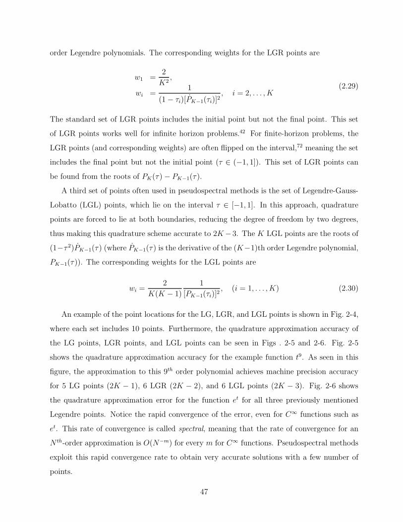
order Legendre polynomials. The corresponding weights for the LGR points are
w1 =2
K2,
wi =1
(1 − τi)[PK−1(τi)]2, i = 2, . . . , K
(2.29)
The standard set of LGR points includes the initial point but not the final point. This set
of LGR points works well for infinite horizon problems.42 For finite-horizon problems, the
LGR points (and corresponding weights) are often flipped on the interval,72 meaning the set
includes the final point but not the initial point (τ ∈ (−1, 1]). This set of LGR points can
be found from the roots of PK(τ) − PK−1(τ).
A third set of points often used in pseudospectral methods is the set of Legendre-Gauss-
Lobatto (LGL) points, which lie on the interval τ ∈ [−1, 1]. In this approach, quadrature
points are forced to lie at both boundaries, reducing the degree of freedom by two degrees,
thus making this quadrature scheme accurate to 2K −3. The K LGL points are the roots of
(1−τ 2)PK−1(τ) (where PK−1(τ) is the derivative of the (K−1)th order Legendre polynomial,
PK−1(τ)). The corresponding weights for the LGL points are
wi =2
K(K − 1)
1
[PK−1(τi)]2, (i = 1, . . . , K) (2.30)
An example of the point locations for the LG, LGR, and LGL points is shown in Fig. 2-4,
where each set includes 10 points. Furthermore, the quadrature approximation accuracy of
the LG points, LGR points, and LGL points can be seen in Figs . 2-5 and 2-6. Fig. 2-5
shows the quadrature approximation accuracy for the example function t9. As seen in this
figure, the approximation to this 9th order polynomial achieves machine precision accuracy
for 5 LG points (2K − 1), 6 LGR (2K − 2), and 6 LGL points (2K − 3). Fig. 2-6 shows
the quadrature approximation error for the function et for all three previously mentioned
Legendre points. Notice the rapid convergence of the error, even for C∞ functions such as
et. This rate of convergence is called spectral, meaning that the rate of convergence for an
N th-order approximation is O(N−m) for every m for C∞ functions. Pseudospectral methods
exploit this rapid convergence rate to obtain very accurate solutions with a few number of
points.
47

−1 −0.5 0 0.5 1support points
equidistantLG pointsLGR pointsLGL points
Figure 2-4: Legendre-Gauss, Legendre-Gauss-Radau, and Legendre-Gauss-Lobatto colloca-tion points for K = 10 on the interval [−1, 1]
0 5 10 15 20 25 3010
−20
10−15
10−10
10−5
100
105
LGLGRLGL
Rel
ativ
eE
rror
Number of support points
Figure 2-5: Accuracy of the quadrature approximation to t9 using LG, LGL, and LGR pointsas the number of points increases
48
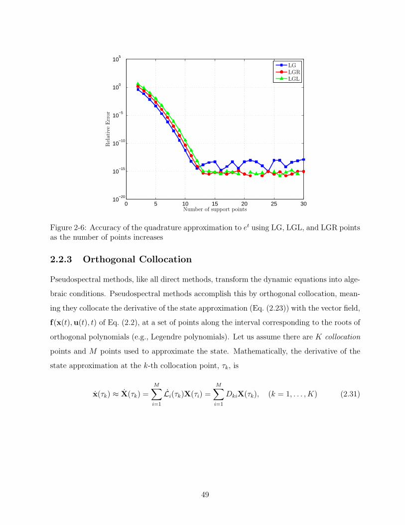
0 5 10 15 20 25 3010
−20
10−15
10−10
10−5
100
105
LGLGRLGL
Rel
ativ
eE
rror
Number of support points
Figure 2-6: Accuracy of the quadrature approximation to et using LG, LGL, and LGR pointsas the number of points increases
2.2.3 Orthogonal Collocation
Pseudospectral methods, like all direct methods, transform the dynamic equations into alge-
braic conditions. Pseudospectral methods accomplish this by orthogonal collocation, mean-
ing they collocate the derivative of the state approximation (Eq. (2.23)) with the vector field,
f(x(t),u(t), t) of Eq. (2.2), at a set of points along the interval corresponding to the roots of
orthogonal polynomials (e.g., Legendre polynomials). Let us assume there are K collocation
points and M points used to approximate the state. Mathematically, the derivative of the
state approximation at the k-th collocation point, τk, is
x(τk) ≈ X(τk) =M∑
i=1
Li(τk)X(τi) =M∑
i=1
DkiX(τk), (k = 1, . . . , K) (2.31)
49
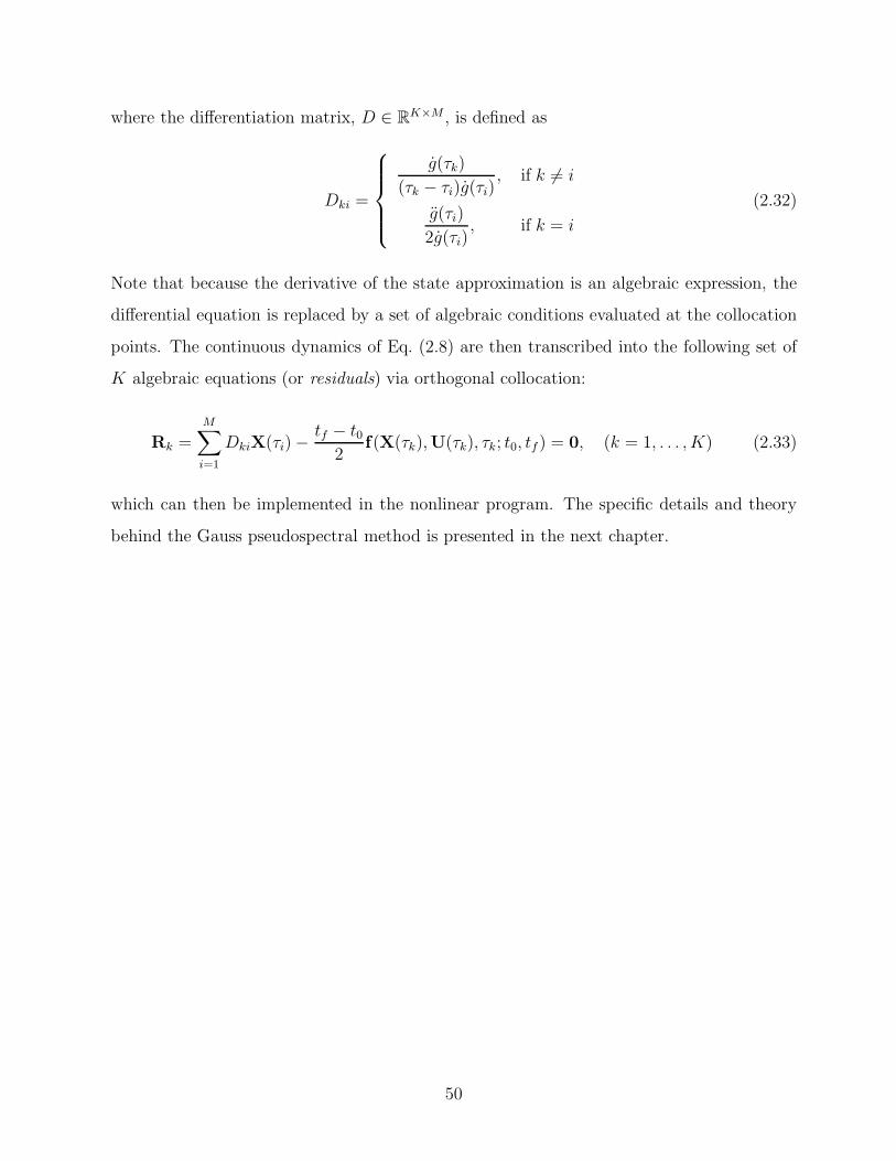
where the differentiation matrix, D ∈ RK×M , is defined as
Dki =
g(τk)
(τk − τi)g(τi), if k 6= i
g(τi)
2g(τi), if k = i
(2.32)
Note that because the derivative of the state approximation is an algebraic expression, the
differential equation is replaced by a set of algebraic conditions evaluated at the collocation
points. The continuous dynamics of Eq. (2.8) are then transcribed into the following set of
K algebraic equations (or residuals) via orthogonal collocation:
Rk =
M∑
i=1
DkiX(τi) −tf − t0
2f(X(τk),U(τk), τk; t0, tf ) = 0, (k = 1, . . . , K) (2.33)
which can then be implemented in the nonlinear program. The specific details and theory
behind the Gauss pseudospectral method is presented in the next chapter.
50

Chapter 3
The Gauss Pseudospectral Method
The Gauss pseudospectral method was originally developed by Benson6 in an effort to im-
prove the costate estimation of the Legendre pseudospectral method. It was originally for-
mulated for optimal control problems involving integral dynamic constraints, but was later
adapted to be used with the more common differential dynamic constraints.
This chapter describes the Gauss pseudospectral method in detail, where the notation
has been streamlined and expanded to include problems with state and/or control path con-
straints. Specific attention is drawn to the costate estimation procedure, and an equivalence
between the NLP multipliers and the discretized costate of the HBVP is mapped out. Fur-
thermore, a new estimate for the boundary control is presented and analyzed. Lastly, the
issue of the convergence of pseudospectral methods is addressed.
3.1 Direct Transcription Formulation
The Gauss pseudospectral transcription converts the transformed continuous Bolza problem
of Chapter 2 into a nonlinear program. This is accomplished using many of the mathematical
approximation tools expained in the second half of Chapter 2.
The Gauss pseudospectral method, like all pseudospectral methods, approximates the
state using a basis of global interpolating polynomials. These global polynomials are based
on a set of discrete points across the interval. One of the primary distinctions between pseu-
dospectral methods is the choice of discrete points used in the NLP formulation. Specifically
51

for the Gauss pseudospectral method, let K = τ1, . . . , τK be the set of K Legendre-Gauss
(LG) points which correspond to the roots of the Kth degree Legendre polynomial, PK(τ),
defined in the previous chapter. These LG points points lie on the interior of the interval
(−1, 1) such that τ1, . . . , τK are strictly increasing. Next, suppose that, for a given value of
K, one can create a superset, K0, that appends the point τ0 = −1 to the set K, for a total of
K + 1 points on the interval [−1, 1). Let x(τ) be the state as a function of the independent
variable τ where τ ∈ [−1, 1], as seen in the transformed continuous Bolza problem. An
approximation to the state, X(τ), is formed with a basis of K + 1 Lagrange interpolating
polynomials Li(τ) (i = 0, . . . , K) as follows:
x(τ) ≈ X(τ) =
K∑
i=0
Li(τ)x(τi) (3.1)
where
Li(τ) =
K∏
j=0,j 6=i
τ − τj
τi − τj(3.2)
The use of Lagrange polynomials results in a state approximation that is equal to the true
state at all the points within K0, or mathematically, x(τi) = X(τi), (i = 0, . . . , K).
Note that the time interval in the transformed optimal control problem spans τ ∈ [−1, 1],
yet the state approximation of Eq. (3.1) does not specifically include a discrete point at
the terminal time, τf = 1. Optimal control problems often include constraints involving
the terminal state, so it is advantagous to include a discrete variable Xf in the nonlinear
program. Therefore, in order to fully discretize the time interval for the NLP, another set
of points, called discretization points or nodes, is created as a superset of K0. The set of
nodes, N , includes the K interior LG points, τ1, . . . , τK , the initial point, τ0 ≡ −1, and the
final point, τf ≡ 1. The state at the final time, Xf , is included in the NLP discretization,
although it is not specifically part of the state approximation of Eq. (3.1). Since Xf is absent
in the state approximation, it must be constrained in other ways to ensure that it satisfies
the state dynamic equations of Eq. (2.8). This is accomplished by including an additional
constraint that relates the final state to the initial state via a Gauss quadrature. According
52

to the state dynamics,
x(τf) = x(τ0) +
∫ 1
−1
f(x(τ),u(τ), τ)dτ (3.3)
which can be discretized and approximated as
X(τf ) −X(τ0) −tf − t0
2
K∑
k=1
wkf(X(τk),U(τk), τk; t0, tf ) = 0 (3.4)
where wk are the Gauss weights and τk are the LG points. At first glance, the non-intuitive
handling of the terminal state seems unnecessarily complicated, however by formulating the
problem in this manner, unique mathematical properties can be derived which allow for a
very accurate approximation to the costate. This is presented more formally in the next
section.
Eq. (3.4) forces the terminal state to satisfy the dynamic constraints, but additional
constraints must be posed to ensure that the entire discrete state satisfies the dynamic
equations. This is accomplished via orthogonal collocation, as described in Chapter 2. Col-
location methods require the dynamic equations of Eq. (2.2) to be satisfied exactly at a set
of collocation points. The left-hand side of the dynamic equations is approximated by differ-
entiating the state approximation of Eq. (3.1) at the Legendre-Gauss points in the manner
of Eq. (2.31) as follows:
x(τk) ≈ X(τk) =
K∑
i=0
Li(τk)X(τi) =
K∑
i=0
DkiX(τk), (k = 1, . . . , K) (3.5)
The differentiation matrix, D ∈ RK×(K+1), can be determined offline from Eq. (2.32), where
g(τ) = (1 + τ)PN(τ).
Dki = Li(τk) =
(1 + τk)PK(τk) + PK(τk)
(τk − τi)[
(1 + τi)PK(τi) + PK(τi)] , i 6= k
(1 + τi)PK(τi) + 2PK(τi)
2[
(1 + τi)PK(τi) + PK(τi)] , i = k
(3.6)
where τk, (k = 1, . . . , K) are the points in the set K, and τi, (i = 0, . . . , K) are the points in
53

the set K0. Unlike many pseudospectral methods, the Gauss pseudospectral method does not
collocate at every point in the discretization set, N . To emphasize this point, the set of LG
points, K, is termed the set of collocation points. Recall the discretization set (N ) contains
the LG points plus the initial point and final point. Therefore, for the Gauss pseudspectral
method, there are two more discretization points than collocation points (K = N − 2). The
K collocation equations require Eq. (3.5) to be equal to the right-hand side of the dynamic
equations at the collocation points:
K∑
i=0
DkiX(τi) −tf − t0
2f(X(τk),U(τk), τk; t0, tf) = 0, (k = 1, . . . , K) (3.7)
As is shown shortly, collocating strictly on the interior of the interval leads to a unique
mathematical equivalence used to approximate the costate.
A discrete approximation for the control, Uk, (k = 1, . . . , K) is required for the col-
location constraints of Eq. (3.7) as well as the quadrature constraint of Eq. (3.4). The
time derivative of the control is not approximated, so the control approximation need not
be of the form Eq. (2.23). In fact, any approximation that has the property u(τk) = Uk,
(k = 1, . . . , K) is an equivalent control approximation in the eyes of the NLP. However, for
consistency, this work approximates the control at the K collocation points using a basis of
K Lagrange interpolating polynomials Li(τ), (i = 1, . . . , K) as
u(τ) ≈ U(τ) =K∑
i=1
Li(τ)U(τi) (3.8)
where τi, (i = 1, . . . , K) are the LG points belonging to the set K.
Lastly, the integral term in the cost functional of Eq. (2.7) can be approximated with a
Gauss quadrature as before, resulting in
J = Φ(X0, t0,Xf , tf ) +tf − t0
2
K∑
k=1
wkg(Xk,Uk, τk; t0, tf ) (3.9)
54

3.1.1 Gauss Pseudospectral Discretization of Transformed Con-
tinuous Bolza Problem
From the previous discussion, the Gauss pseudospectral discretization of the transformed
continuous Bolza optimal control problem in Chap 2 can now be stated formally. Determine
the discretized state, Xi, i ∈ N , control, Uk, k ∈ K, initial time, t0, and final time, tf that
minimizes the cost function
J = Φ(X0, t0,Xf , tf ) +tf − t0
2
K∑
k=1
wkg(Xk,Uk, τk; t0, tf ) (3.10)
subject to the algebraic collocation constraints expressed as a residual function,
Rk ≡K∑
i=0
DkiXi −tf − t0
2f(Xk,Uk, τk; t0, tf) = 0 (k = 1, . . . , N) (3.11)
quadrature constraint expressed as a residual,
Rf ≡ Xf −X0 −tf − t0
2
K∑
k=1
wkf(Xk,Uk, τk; t0, tf) = 0 (3.12)
boundary constraint,
φ(X0, t0,Xf , tf) = 0 (3.13)
and path constraint,
C(Xk,Uk, τk; t0, tf) ≤ 0 (k = 1, . . . , N) (3.14)
The cost function of Eq. (3.10) and the constraints of Eq. (3.11)–(3.14) define an NLP whose
solution is an approximate solution to the continuous Bolza problem.
To recap, the variables that are used in the GPM discretization are as follows:
NLP Variables Corresponding to State: (X0,X1, . . . ,XK ,Xf)
NLP Variables Corresponding to Control: (U1, . . . ,UK)
55

Similarly, the constraints in the GPM are as follows:
Constraints Corresponding to Dynamics: (R1, . . . ,RK ,Rf )
Constraints Corresponding to Path Constraints: (C1, . . . ,CK)
Constraints Corresponding to Boundary Conditions: φ
3.1.2 A Comment on the Final State: Xf
As seen in the previous section, the state is discretized at all N discretization points, but
the actual state approximation of Eq. (3.1) includes only N − 1 points in the set K0. The
final state is not explicitly in the state approximation. It is, however, implicitly in the state
approximation due to the quadrature constraint of Eq. (3.4). Although it is not immediately
obvious, the inclusion of the quadrature constraint produces the same value for Xf as one
would get by extrapolating the state approximation of Eq. (3.1) to tf . In this section,
it is shown mathematically that these two expressions are consistent with one another.
Specifically, it is shown that the NLP final state, Xf is the same as the extrapolated state
X(tf):
Lemma 1. Using the Gauss pseudospectral transcription for an optimal control problem, the
following two formulations for Xf are equivalent:
Xf = X0 +tf − t0
2
K∑
k=1
wkf(Xk,Uk, τk; t0, tf ) (3.15)
and
Xf = X(tf) =K∑
i=0
X(ti)Li(tf), (3.16)
Proof of Lemma 1. Beginning with Eq. (3.15):
Xf = X0 +tf − t0
2
K∑
k=1
wkf(Xk,Uk, τk; t0, tf ) (3.17)
From the collocation constraints of Eq. (3.11), the vector field at the Gauss points is equal
to the derivative of the state approximation, therefore f(Xk,Uk, τk; t0, tf) can be replaced in
56

Eq. (3.17):
Xf = X0 +
K∑
k=1
wk
(
K∑
i=0
X(τi)Dki
)
(3.18)
Recall that Dki = Li(τk). Hence, Eq. (3.18) is a Gauss quadrature for a polynomial of degree
less than 2K − 1 and can be replaced exactly with an integral
Xf = X0 +
∫ 1
−1
K∑
i=0
X(τi)Li(τ)dτ (3.19)
This integral can be evaluated, resulting in
Xf = X0 +
K∑
i=0
X(τi)Li(τf ) −K∑
i=0
X(τi)Li(τ0) (3.20)
According to the definition of Lagrange polynomials in Eq. (3.2), the final term in Eq. (3.20)
is equal to X0, so the first and last terms cancel, resulting in
Xf =
K∑
i=0
X(τi)Li(τf ) (3.21)
which simplifies to
Xf = X(tf) (3.22)
from Eq. (3.16).
2
The state approximation and the quadrature constraint are consistent with one another
and do not produce conflicting values for the state at the final time.
It is noted that in his original formulation, Benson did not explicitly include Xf or
Eq. (3.12) into the NLP, but rather used Eq. (3.12) to eliminate Xf from the problem. This
has the benefit of reducing the number of NLP nodes by one, but also makes the other
constraints more complicated. For example, if Xf is not explicitly in the discretization,
then any simple terminal constraint on the state would be a function of the state at all the
discretization points in the NLP according to Eq. (3.12). Because simple terminal constraints
57

are often found in optimal control problems, this work retains that simplicity by explicitly
including Xf and Eq. (3.12) in the NLP formulation.
3.1.3 Discontinuities & Phases
Some optimal control problems have known discontinuities in either the state or control.
Common examples are a mass drop during a launch vehicle ascent problem, or a “bang-
bang” control solution. The spectral accuracy described in Chapter 2 only applies to smooth
problems, meaning the primary advantage of using a global polynomial approximation is
eliminated for discontinuous problems. Chapter 5 discusses this effect in more detail. How-
ever, for problems with known discontinuities, a common procedure to recover the spectral
accuracy is to divide the trajectory into phases, where the dynamics are transcribed within
each phase and then connected together by additional phase interface (a.k.a linkage) con-
straints.85,95 Other approaches involve using a smoothing filter34 to eliminate the oscillatory
Gibb’s phenomenon often associated with a polynomial approximation to a discontinuous
function.
The Gauss pseudospectral method has been used to solve several multi-phase problems
(see Ref. 6,66,68). The extension to a P -phase problem involves repeating the structure for
the one-phase formulation P times. In addition, the terminal constraints for the first phase,
the initial and terminal constraints for the interior phases, and the initial constraints for the
P th phase are re-characterized as interior point constraints. These interior point constraints
include any continuity conditions in the state or time between adjacent phases. For our
formulation, it is assumed that the control is allowed to be discontinuous across phases, but
this too can be constrained if necessary. Eq. (3.13) of Section 3.1.1 can then be replaced by
the following set of equations:
L(1)(X(1)0 , t
(1)0 ) = 0,
L(r+1)(r) (X
(r)f , t
(r)f ,X
(r+1)0 , t
(r+1)0 ) = 0,
L(P )(X(P )f , t
(P )f ) = 0
(3.23)
where r = 1, . . . , P − 1 phases. It is noted that these phases do not need to be sequential,
58
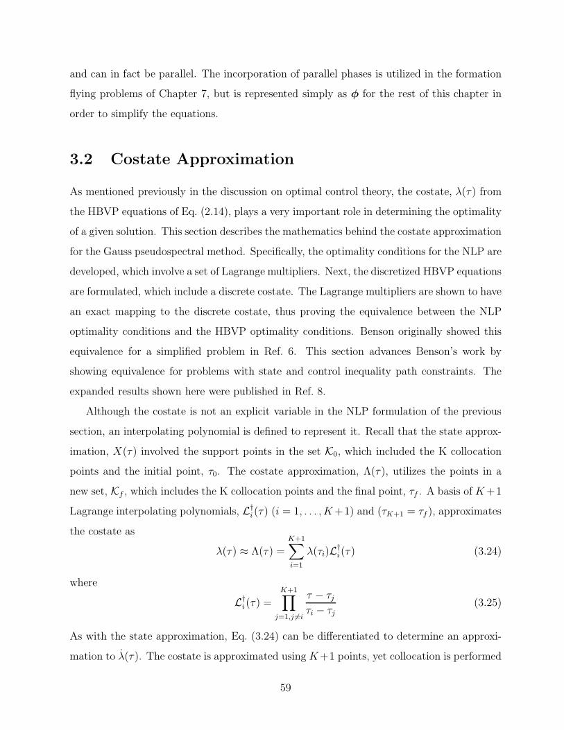
and can in fact be parallel. The incorporation of parallel phases is utilized in the formation
flying problems of Chapter 7, but is represented simply as φ for the rest of this chapter in
order to simplify the equations.
3.2 Costate Approximation
As mentioned previously in the discussion on optimal control theory, the costate, λ(τ) from
the HBVP equations of Eq. (2.14), plays a very important role in determining the optimality
of a given solution. This section describes the mathematics behind the costate approximation
for the Gauss pseudospectral method. Specifically, the optimality conditions for the NLP are
developed, which involve a set of Lagrange multipliers. Next, the discretized HBVP equations
are formulated, which include a discrete costate. The Lagrange multipliers are shown to have
an exact mapping to the discrete costate, thus proving the equivalence between the NLP
optimality conditions and the HBVP optimality conditions. Benson originally showed this
equivalence for a simplified problem in Ref. 6. This section advances Benson’s work by
showing equivalence for problems with state and control inequality path constraints. The
expanded results shown here were published in Ref. 8.
Although the costate is not an explicit variable in the NLP formulation of the previous
section, an interpolating polynomial is defined to represent it. Recall that the state approx-
imation, X(τ) involved the support points in the set K0, which included the K collocation
points and the initial point, τ0. The costate approximation, Λ(τ), utilizes the points in a
new set, Kf , which includes the K collocation points and the final point, τf . A basis of K +1
Lagrange interpolating polynomials, L†i (τ) (i = 1, . . . , K +1) and (τK+1 = τf ), approximates
the costate as
λ(τ) ≈ Λ(τ) =K+1∑
i=1
λ(τi)L†i(τ) (3.24)
where
L†i(τ) =
K+1∏
j=1,j 6=i
τ − τj
τi − τj(3.25)
As with the state approximation, Eq. (3.24) can be differentiated to determine an approxi-
mation to λ(τ). The costate is approximated using K+1 points, yet collocation is performed
59

at the K collocation points using
λ(τk) ≈ Λ(τk) =
K+1∑
i=1
λ(τi)D†ki (k = 1, . . . , K) (3.26)
where D†ki = L†
i(τk) represents the elements of the differential approximation matrix D† ∈R
K×K+1. D† is referred to as the adjoint of the differential approximation matrix D. Gauss
weights are used to prove the following lemma that relates elements of the differential ap-
proximation matrix, D, to elements of the adjoint differential approximation matrix, D†, as
originally shown in Ref. 6:
Lemma 2. [6] The relationship between elements in the differential approximation matrix
D and elements in its adjoint D† is
Dik = −wk
wiD†
ki (i, k = 1, . . . , K) (3.27)
where wi and wk, (i, k = 1, . . . , K) are the Gauss weights.29 Notice the elements of D cor-
responding to the initial point, τ0 (the first column of D), and elements of D† corresponding
to the final point, τf (the last column of D†), are omitted in this relationship.
Proof of Lemma 2 (6). Consider the integration by parts formula for the product of p(τ)
and q(τ) with τ ∈ [−1, 1] where p(τ) and q(τ) are defined to be polynomials of degree K, i.e.,
∫ 1
−1
p(τ)q(τ)dτ = p(τ)q(τ)∣
∣
∣
1
−1−∫ 1
−1
p(τ)q(τ)dτ
Because p(τ) and q(τ) are polynomials of degree K, the functions p(τ)q(τ) and p(τ)q(τ) are
polynomials of degree 2K − 1 and, thus, can be replaced exactly by a Gauss quadrature.29
Then, using the exact derivatives of the polynomials p(τ) and q(τ) at the Gauss points in
Eqs. (3.5) and (3.26), respectively, the integration by parts formula is replaced exactly by
K∑
j=1
[
K∑
l=0
Djlp(τl)
]
q(τj)wj =
[p(1)q(1) − p(−1)q(−1)] −K∑
j=1
p(τj)
[
K+1∑
l=1
D†jlq(τl)
]
wj
(3.28)
60
Because Eq. (3.28) must hold for all polynomials p(τ) and q(τ) of degree K or less, it must
hold for the set of Kth degree Lagrange interpolating polynomials Lp(τ) (p = 0, . . . , K) and
L†q(τ) (q = 1, . . . , K+1) as defined in Eqs. (3.2) and (3.25). To show the relationship between
the elements of the differential approximation matrix D and the elements of the adjoint D†,
a subset of these Lagrange polynomials, Lk(τ) and L†i(τ) (i, k = 1, . . . , K) from Eqs. (3.2)
and (3.25), respectively, are substituted into Eq. (3.28) to obtain
K∑
j=1
[
K∑
l=0
DjlLk(τl)
]
L†i(τj)wj =
[
Lk(1)L†i(1) − Lk(−1)L†
i (−1)]
−K∑
j=1
Lk(τj)
[
K+1∑
l=1
D†jlL†
i (τl)
]
wj
(3.29)
Now from the properties of Lagrange polynomials in Eq. (2.25) it is seen that
Lk(−1) = 0 (k = 1, . . . , K)
L†i(1) = 0 (i = 1, . . . , K)
Eq. (3.29) then simplifies to
K∑
j=1
K∑
l=1
DjlLk(τl)L†i(τj)wj = −
K∑
j=1
K∑
l=1
D†jlLk(τj)L†
i(τl)wj (3.30)
Then, once again using the Lagrange polynomial properties of Eq. (2.25) in Eq. (3.30), it can
be seen that the product Lk(τl)L†i(τj) is zero unless k = l and i = j. Similarly, the product
Lk(τj)L†i(τl) is zero unless k = j and i = l. Therefore, the following result is obtained at the
Gauss points:
Dikwi = −D†kiwk (i, k = 1, . . . , K) (3.31)
Rearranging Eq. (3.31) yields Eq. (3.27).
2
The following relationships involving the differentiation matrix are also important in the
costate analysis of the Gauss pseudospectral transcription method, originally shown in Ref. 6.
61

Lemma 3. [6] The elements of the differential approximation matrix, D, corresponding to
the LG points are related to the elements D corresponding to the initial time, τ0, by the
equation
Di,0 = −K∑
k=1
Dik (3.32)
Proof of Lemma 3 (6). This relationship can be shown by examining the derivative of a
constant function, f(t) = c. Applying the differential approxmation matrix results in
f(ti) = cDi,0 + c
K∑
k=1
Dik = 0 (3.33)
This relation is exact for all values of K because the function f(t) = c is a polynomial of
degree 0. The result can be simplified to Eq. (3.32).
2
A similar relationship can be drawn for the adjoint differentiation matrix, D†.
Lemma 4. [6] The elements of the adjoint differential approximation matrix, D†, corre-
sponding to the LG points are related to the elements D† corresponding to the final time, τf ,
by the equation
D†i,K+1 = −
K∑
k=1
D†ik (3.34)
Proof of Lemma 4 (6). This relationship can also be shown by examining the derivative
of a constant function, f(t) = c. See Lemma 3.
2
3.2.1 KKT Conditions of the Transcribed NLP
The solution to a nonlinear program satisfies a set of first-order optimality conditions called
the Karush-Kuhn-Tucker (KKT) conditions. The KKT conditions corresponding to the NLP
described in Section 3.1.1 can be obtained using the augmented cost function or Lagrangian.9
The augmented cost function is formed using the Lagrange multipliers Λk ∈ Rn, µk ∈ R
c,
62
k = 1, . . . , K, ΛF ∈ Rn, and ν ∈ R
q as
Ja = Φ(X0, t0,Xf , tf) +tf − t0
2
K∑
k=1
wkg(Xk,Uk, τk; t0, tf) − νT φ(X0, t0,Xf , tf )
−K∑
k=1
µTk C(Xk,Uk, τk; t0, tf ) −
K∑
k=1
ΛT
k
(
K∑
i=0
DkiXi −tf − t0
2f(Xk,Uk, τk; t0, tf)
)
−ΛF
T
(
Xf − X0 −tf − t0
2
K∑
k=1
wkf(Xk,Uk, τk; t0, tf )
)
(3.35)
where the tilde notation is used to highlight multipliers related to the solution of the NLP.
The KKT conditions are found by setting equal to zero the derivatives of the Lagrangian
with respect to X0, Xk, Xf , Uk, Λk, µk, ΛF , ν, t0, and tf .9
First, setting equal to zero the partial derivatives of the Lagrangian with respect to the
Lagrange multipliers, Λk, µk, ΛF , and ν results in Eqs. (3.11)–(3.14). Next, suppose
C(x,u, τ ; t0, tf) =
C1
C2
...
Cc
(3.36)
Then, applying the complementary slackness condition,9
µjk = 0 , when Cjk < 0
µjk ≤ 0 , when Cjk = 0
(j = 1, · · · , c), (k = 1, · · · , K) (3.37)
where Cjk ≡ Cj(Xk,Uk, τk; t0, tf) and µjk is the jth component of µk.
The partial derivative of the augmented cost function with respect to the state at the kth
LG point, Xk, k = 1, . . . , K, is given as
∂Ja
∂Xk
=tf − t0
2wk
∂gk
∂Xk
− µTk
∂Ck
∂Xk
−K∑
i=1
DikΛT
i +
+tf − t0
2Λ
T
k
∂fk∂Xk
+tf − t0
2wkΛ
T
F
∂fk∂Xk
(3.38)
63

where simplifying notation gk ≡ g(Xk,Uk, τk; t0, tf), fk ≡ f(Xk,Uk, τk; t0, tf), and Ck ≡C(Xk,Uk, τk; t0, tk) is used. Setting Eq. (3.38) equal to zero and dividing through by wk
results in
0T =tf − t0
2
[
∂gk
∂Xk
− 2
tf − t0
µTk
wk
∂Ck
∂Xk
+
(
ΛT
k
wk
+ ΛT
F
)
∂fk∂Xk
]
−K∑
i=1
DikΛ
T
i
wk
(3.39)
Applying Lemma 2 to Eq. (3.39) and adding and subtracting the termK∑
i=1
D†kiΛ
T
F , results in
0T =tf − t0
2
[
∂gk
∂Xk− 2
tf − t0
µTk
wk
∂Ck
∂Xk+
(
ΛT
k
wk+ Λ
T
F
)
∂fk∂Xk
]
+K∑
i=1
D†ki
(
ΛT
i
wi+ Λ
T
F
)
−K∑
i=1
D†kiΛ
T
F
(3.40)
Applying Lemma 4 to the last term in Eq. (3.40) results in
0T =tf − t0
2
[
∂gk
∂Xk
− 2
tf − t0
µTk
wk
∂Ck
∂Xk
+
(
ΛT
k
wk
+ ΛT
F
)
∂fk∂Xk
]
+K∑
i=1
D†ki
(
ΛT
i
wi
+ ΛT
F
)
+ D†k,K+1Λ
T
F
(3.41)
The next KKT condition is found by computing the partial derivative of the augmented cost
function with respect to the control Uk as
∂Ja
∂Uk=
tf − t02
wk∂gk
∂Uk− µT
k
∂Ck
∂Uk
+tf − t0
2Λ
T
k
∂fk∂Uk
+tf − t0
2wkΛ
T
F
∂fk∂Uk
(3.42)
Setting Eq. (3.42) equal to zero and multiplying through by2
(tf − t0)wk
, gives
0T =∂gk
∂Uk+
(
ΛT
k
wk+ Λ
T
F
)
∂fk∂Uk
− 2
tf − t0
µTk
wk
∂Ck
∂Uk(3.43)
64
The next KKT condition is found by computing the partial derivative of the augmented cost
function with respect to the initial state, X0, as
∂Ja
∂X0
=∂Φ
∂X0
− νT ∂φ
∂X0
−K∑
k=1
Dk,0ΛT
k + ΛT
F (3.44)
Applying Lemmas 2 and 3 to Eq. (3.44),
0T =∂Φ
∂X0− νT ∂φ
∂X0−
K∑
k=1
K∑
i=1
wi
wkD†
ikΛT
k + ΛT
F (3.45)
Adding and subtracting the term
K∑
i=1
wi
K∑
k=1
D†ikΛF in Eq. (3.45) yields
0T =∂Φ
∂X0− νT ∂φ
∂X0+ Λ
T
F
−K∑
i=1
wi
[
K∑
k=1
D†ik
(
ΛT
k
wk+ Λ
T
F
)
−K∑
k=1
D†ikΛ
T
F
] (3.46)
Applying Lemma 4 to Eq. (3.46) results in
0T =∂Φ
∂X0− νT ∂φ
∂X0+ Λ
T
F
−K∑
i=1
wi
[
K∑
k=1
D†ik
(
ΛT
k
wk+ Λ
T
F
)
+ D†i,K+1Λ
T
F
] (3.47)
Suppose now that the new variable, Λ0, is defined as
ΛT
0 ≡ − ∂Φ
∂X0
+ νT ∂φ
∂X0
(3.48)
Then, replacing the term in the square brackets in Eq. (3.47) using (3.41) produces
0T = −ΛT
0 + ΛT
F
+tf − t0
2
K∑
i=1
wi
[
∂gi
∂Xi− 2
tf − t0
µTi
wi
∂Ci
∂Xi+
(
ΛT
i
wi+ Λ
T
F
)
∂fi∂Xi
]
(3.49)
65

The next KKT condition is found by taking the partial derivative of the augmented cost
function with respect to the final state, Xf , as
0T =∂Ja
∂Xf
=∂Φ
∂Xf
− νT ∂φ
∂Xf
− ΛT
F (3.50)
The last two KKT conditions are found by computing the partial derivatives of the aug-
mented cost function with respect the initial and final times. First, computing the partial
derivative of the augmented cost function with respect to the initial time results in
∂Ja
∂t0=
∂Φ
∂t0− 1
2
K∑
k=1
wkgk +tf − t0
2
K∑
k=1
wk∂gk
∂t0− νT ∂φ
∂t0
−K∑
k=1
µTk
∂Ck
∂t0− 1
2
K∑
k=1
ΛT
k fk +tf − t0
2
K∑
k=1
ΛT
k
∂fk∂t0
−1
2
K∑
k=1
wkΛT
F fk +tf − t0
2
K∑
k=1
wkΛT
F
∂fk∂t0
(3.51)
Note that the functions g, f, and C are now explicit functions of t0 and tf due to the
transformation from t ∈ [t0, tf ] to τ ∈ [−1, 1] in Eq. (2.6). The term1
2
K∑
k=1
wk2
tf − t0
µTk
wk
Ck
(which equals zero due to the complementary slackness condition of Eq. (3.37)) is added to
Eq. (3.51). The resulting equation is
0 =∂Φ
∂t0− νT ∂φ
∂t0− 1
2
K∑
k=1
wk
[
gk +
(
ΛT
k
wk+ Λ
T
F
)
fk −2
tf − t0
µTk
wkCk
]
+tf − t0
2
K∑
k=1
wk
[
∂gk
∂t0+
(
ΛT
k
wk+ Λ
T
F
)
∂fk∂t0
− 2
tf − t0
µTk
wk
∂Ck
∂t0
]
(3.52)
Similarly, computing the partial derivative of the augmented cost function with respect to
66

the final time produces
∂Ja
∂tf=
∂Φ
∂tf+
1
2
K∑
k=1
wkgk +tf − t0
2
K∑
k=1
wk∂gk
∂tf− νT ∂φ
∂tf
−K∑
k=1
µTk
∂Ck
∂tf+
1
2
K∑
k=1
ΛT
k fk +tf − t0
2
K∑
k=1
ΛT
k
∂fk∂tf
+1
2
K∑
k=1
wkΛT
F fk +tf − t0
2
K∑
k=1
wkΛT
F
∂fk∂tf
(3.53)
Combining terms and subtracting the complementary slackness term results in
0 =∂Φ
∂tf− νT ∂φ
∂tf+
1
2
K∑
k=1
wk
[
gk +
(
ΛT
k
wk
+ ΛT
f
)
fk −2
tf − t0
µTk
wk
Ck
]
+tf − t0
2
K∑
k=1
wk
[
∂gk
∂tf+
(
ΛT
k
wk+ Λ
T
f
)
∂fk∂tf
− 2
tf − t0
µTk
wk
∂Ck
∂tf
](3.54)
The solution to the NLP of Eqs. (3.10)–(3.12) must satisfy the set of KKT conditions
67

described below:
K∑
i=0
XiDki =tf − t0
2fk (3.55)
K∑
i=1
(
ΛT
i
wi+ Λ
T
F
)
D†ki + Λ
T
F D†k,K+1 =
tf − t02
(
− ∂gk
∂Xk−(
ΛT
k
wk+ Λ
T
F
)
∂fk∂Xk
+2
tf − t0
µTk
wk
∂Ck
∂Xk
)(3.56)
0T =∂gk
∂Uk
+
(
ΛT
k
wk
+ ΛT
F
)
∂fk∂Uk
− 2
tf − t0
µTk
wk
∂Ck
∂Uk
(3.57)
φ(X0, t0,Xf , tf ) = 0 (3.58)
ΛT
0 = − ∂Φ
∂X0
+ νT ∂φ
∂X0
(3.59)
ΛT
F =∂Φ
∂Xf
− νT ∂φ
∂Xf
(3.60)
−tf − t02
K∑
k=1
wk∂Hk
∂t0+
1
2
K∑
k=1
wkHk =∂Φ
∂t0− νT ∂φ
∂t0(3.61)
tf − t02
K∑
k=1
wk∂Hk
∂tf+
1
2
K∑
k=1
wkHk = −∂Φ
∂tf+ νT ∂φ
∂tf(3.62)
Ck ≤ 0 (3.63)
µjk = 0 , when Cjk < 0 (3.64)
µjk ≤ 0 , when Cjk = 0 (3.65)
Xf = X0 +(tf − t0)
2
K∑
k=1
wkfk (3.66)
ΛT
F = ΛT
0 +tf − t0
2
K∑
k=1
wk
(
− ∂gk
∂Xk−(
ΛT
k
wk+ Λ
T
F
)
∂fk∂Xk
+2
tf − t0
µTk
wk
∂Ck
∂Xk
)
(3.67)
where the shorthand notation gk ≡ g(Xk,Uk, τk; t0, tf ), fk ≡ f(Xk,Uk, τk; t0, tf), Hk ≡H(Xk,Λk, µk,Uk, τk; t0, tf), and Cjk ≡ Cj(Xk,Uk, τk; t0, tf) is used. Note that the discrete
augmented Hamiltonian, Hk, is defined here as
Hk ≡ gk +
(
ΛT
k
wk+ Λ
T
F
)
fk −2
tf − t0
µTk
wkCk (3.68)
68

3.2.2 Gauss Pseudospectral Discretization of the First-Order Nec-
essary Conditions
This section describes in detail the discretized equations resulting from the Gauss pseu-
dospectral transcription of the first-order necessary conditions of the HBVP in Chapter 2.
In practice this step is not necessary in order to solve the problem, but by transcribing the
HBVP, one can extract a mapping between this set of equations and the equations in the
previous section. The entire set of continuous-time necessary conditions of the transformed
Bolza problem in Eq. (2.14) are discretized as follows. The state, control, and costate are
approximated using Eqs. (3.1), (3.8), and (3.24), respectively. The continuous-time first-
order optimality conditions of Eq. (2.14) are discretized using the variables X0 ≡ X(τ0),
Xk ≡ X(τk) ∈ Rn, (k = 1, . . . , K), and Xf ≡ X(τf ) for the state, Uk ≡ U(τk) ∈ R
m, (k =
1, . . . , K) for the control, Λ0 ≡ Λ(τ0), Λk ≡ Λ(τk) ∈ Rn, (k = 1, . . . , K), and Λf ≡ Λ(τf )
for the costate, and µk ≡ µ(τk) ∈ Rc, (k = 1, . . . , K), for the Lagrange multiplier associated
with the path constraints. The other unknown variables in the problem are the initial and
final times, t0 ∈ R, tf ∈ R, and the Lagrange multiplier, ν ∈ Rq. The total number of
variables is then given as (2n + m + c)K + 4n + q + 2. These variables are used to discretize
the continuous necessary conditions of Eq. (2.14). Recall that the derivative of the state is
approximated using Lagrange polynomials based on K + 1 points consisting of the K LG
points and the initial time, τ0, while the derivative of the costate is approximated using La-
grange polynomials based on K +1 points consisting of the K LG points and the final time,
τf . The resulting algebraic equations that approximate the continuous necessary conditions
69

are given as
K∑
i=0
XiDki =tf − t0
2fk (3.69)
K∑
i=1
ΛTi D†
ki + ΛTf D†
k,K+1 =tf − t0
2
(
− ∂gk
∂Xk− ΛT
k
∂fk∂Xk
+ µTk
∂Ck
∂Xk
)
(3.70)
0T =∂gk
∂Uk+ ΛT
k
∂fk∂Uk
− µTk
∂Ck
∂Uk(3.71)
φ(X0, t0,Xf , tf ) = 0 (3.72)
ΛT0 = − ∂Φ
∂X0+ νT ∂φ
∂X0(3.73)
ΛTf =
∂Φ
∂Xf− νT ∂φ
∂Xf(3.74)
−tf − t02
K∑
k=1
wk∂Hk
∂t0+
1
2
K∑
k=1
wkHk =∂Φ
∂t0− νT ∂φ
∂t0(3.75)
tf − t02
K∑
k=1
wk∂Hk
∂tf+
1
2
K∑
k=1
wkHk = −∂Φ
∂tf+ νT ∂φ
∂tf(3.76)
µjk = 0 , when Cjk < 0 (3.77)
µjk ≤ 0 , when Cjk = 0 (3.78)
for k = 1, . . . , K and j = 1, . . . , c. Note that the augmented Hamiltonian, Hk, is defined as
Hk ≡ gk + ΛTk fk − µT
k Ck (3.79)
The final two equations that are required are
Xf = X0 +tf − t0
2
K∑
k=1
wkfk (3.80)
ΛTf = ΛT
0 +tf − t0
2
K∑
k=1
wk
(
− ∂gk
∂Xk
− ΛTk
∂fk∂Xk
+ µTk
∂Ck
∂Xk
)
(3.81)
Equations (3.80) and (3.81) are required in order to link the initial and final state and
costate with the interior points. The total number of equations in Eqs. (3.69)–(3.81) is
(2n+m+ c)K +4n+ q +2 (the same as the number of unknown variables). The solution to
70

these nonlinear algebraic equations is an indirect solution to the optimal control problem.
Note that Eqs. (3.75)-(3.76) were derived from the original necessary conditions using
the relationships:
H(t0) = −tf − t02
∫ 1
−1
∂H∂t0
dτ +1
2
∫ 1
−1
Hdτ (3.82)
H(tf ) =tf − t0
2
∫ 1
−1
∂H∂tf
dτ +1
2
∫ 1
−1
Hdτ (3.83)
3.2.3 Costate Mapping Theorem
A costate estimate for the Bolza problem results from a comparison of the discretized nec-
essary conditions from Section 3.2.2 to the optimality or Karush-Kuhn-Tucker conditions
of the nonlinear programming problem in Section 3.2.1. The theorem presented here is an
expansion of the one developed in Ref. 6 and is published in Ref. 8.
Theorem 1 (Gauss Pseudospectral Costate Mapping Theorem). The Karush-Kuhn-
Tucker (KKT) conditions of the NLP are exactly equivalent to the discretized form of the
continuous first-order necessary conditions of the Bolza problem when using the Gauss pseu-
dospectral discretization. Furthermore a costate estimate at the initial time, final time, and
the Gauss points can be found from the KKT multipliers, Λk, µk, ΛF , and ν,
Λk =Λk
wk+ ΛF
µk =2
tf − t0
µk
wk
ν = ν
Λ0 = Λ0 , Λ(tf ) = ΛF
(3.84)
Proof of Theorem 1. Using the substitution of Eq. (3.84), it is seen that Eqs. (3.55)–(3.67)
are exactly the same as Eqs. (3.69)–(3.81).
2
Theorem 1 indicates that solving the NLP derived from the Gauss pseudospectral tran-
scription of the optimal control problem is equivalent to applying the Gauss pseudospectral
71
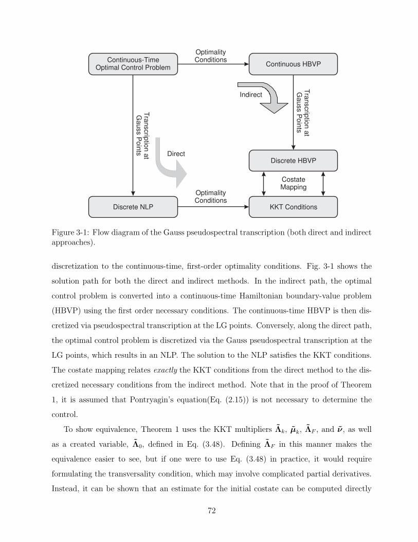
Tra
nscrip
tion a
tG
auss P
oin
ts
OptimalityConditions
OptimalityConditions
Tra
nscrip
tion a
tG
auss P
oin
ts
Continuous-TimeOptimal Control Problem
Continuous HBVP
Discrete HBVP
KKT Conditions
CostateMapping
Indirect
Direct
Discrete NLP
Figure 3-1: Flow diagram of the Gauss pseudospectral transcription (both direct and indirectapproaches).
discretization to the continuous-time, first-order optimality conditions. Fig. 3-1 shows the
solution path for both the direct and indirect methods. In the indirect path, the optimal
control problem is converted into a continuous-time Hamiltonian boundary-value problem
(HBVP) using the first order necessary conditions. The continuous-time HBVP is then dis-
cretized via pseudospectral transcription at the LG points. Conversely, along the direct path,
the optimal control problem is discretized via the Gauss pseudospectral transcription at the
LG points, which results in an NLP. The solution to the NLP satisfies the KKT conditions.
The costate mapping relates exactly the KKT conditions from the direct method to the dis-
cretized necessary conditions from the indirect method. Note that in the proof of Theorem
1, it is assumed that Pontryagin’s equation(Eq. (2.15)) is not necessary to determine the
control.
To show equivalence, Theorem 1 uses the KKT multipliers Λk, µk, ΛF , and ν, as well
as a created variable, Λ0, defined in Eq. (3.48). Defining ΛF in this manner makes the
equivalence easier to see, but if one were to use Eq. (3.48) in practice, it would require
formulating the transversality condition, which may involve complicated partial derivatives.
Instead, it can be shown that an estimate for the initial costate can be computed directly
72
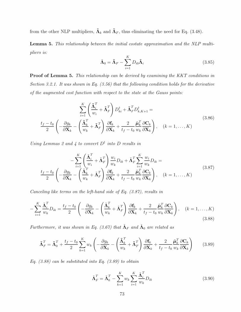
from the other NLP multipliers, Λk and ΛF , thus eliminating the need for Eq. (3.48).
Lemma 5. This relationship between the initial costate approximation and the NLP multi-
pliers is:
Λ0 = ΛF −K∑
i=1
Di0Λi (3.85)
Proof of Lemma 5. This relationship can be derived by examining the KKT conditions in
Section 3.2.1. It was shown in Eq. (3.56) that the following condition holds for the derivative
of the augmented cost function with respect to the state at the Gauss points:
K∑
i=1
(
ΛT
i
wi
+ ΛT
F
)
D†ki + Λ
T
F D†k,K+1 =
tf − t02
(
− ∂gk
∂Xk−(
ΛT
k
wk+ Λ
T
F
)
∂fk∂Xk
+2
tf − t0
µTk
wk
∂Ck
∂Xk
)
, (k = 1, . . . , K)
(3.86)
Using Lemmas 2 and 4 to convert D† into D results in
−K∑
i=1
(
ΛT
i
wi+ Λ
T
F
)
wi
wkDik + Λ
T
F
K∑
i=1
wi
wkDik =
tf − t02
(
− ∂gk
∂Xk−(
ΛT
k
wk+ Λ
T
F
)
∂fk∂Xk
+2
tf − t0
µTk
wk
∂Ck
∂Xk
)
, (k = 1, . . . , K)
(3.87)
Canceling like terms on the left-hand side of Eq. (3.87), results in
−K∑
i=1
ΛT
i
wk
Dik =tf − t0
2
(
− ∂gk
∂Xk
−(
ΛT
k
wk
+ ΛT
F
)
∂fk∂Xk
+2
tf − t0
µTk
wk
∂Ck
∂Xk
)
, (k = 1, . . . , K)
(3.88)
Furthermore, it was shown in Eq. (3.67) that ΛF and Λ0 are related as
ΛT
F = ΛT
0 +tf − t0
2
K∑
k=1
wk
(
− ∂gk
∂Xk−(
ΛT
k
wk+ Λ
T
F
)
∂fk∂Xk
+2
tf − t0
µTk
wk
∂Ck
∂Xk
)
(3.89)
Eq. (3.88) can be substituted into Eq. (3.89) to obtain
ΛT
F = ΛT
0 −K∑
k=1
wk
K∑
i=1
ΛT
i
wk
Dik (3.90)
73
which can be rewritten as
ΛF = Λ0 −K∑
k=1
K∑
i=1
ΛiDik (3.91)
Note that Λi is independent of the summation over the index k. Consequently, Eq. (3.91)
further simplifies to
ΛF = Λ0 −K∑
i=1
Λi
K∑
k=1
Dik (3.92)
Then, applying Lemma 3 gives
ΛF = Λ0 +
K∑
i=1
ΛiDi0 (3.93)
Rearranging,
Λ0 = ΛF −K∑
i=1
ΛiDi0 (3.94)
2
This approximation for the initial costate has a very small computational cost associated
with it, and is preferred in practice over the transversality condition of Eq. (3.48).
3.3 Convergence
The equivalence described in the previous section provides a way to relate the discrete direct
transcription with the discrete indirect transcription of the optimal control problem. Yet
what is still missing is a proof that shows that a solution to the discrete NLP converges to
the optimal solution of the original, continuous-time optimal control problem. This is by no
means a trivial proof, and is currently being studied by several researchers.36,49, 71
Most discussions on convergence in the literature refer to the ability of a numerical inte-
grator to converge to the true solution when integrating a system of differential equations.
Euler, trapezoidal, and Runge-Kutta methods all have certain convergence properties.2,44
However, convergence of an integration method does not necessarily mean that the same
discretization scheme will converge when used to solve an optimal control problem. Hager56
showed that a “convergent” Runge-Kutta method may not actually converge to the contin-
74

uous optimal solution when used to solve an optimal control problem. Conversely, Betts15
showed that a “nonconvergent” scheme could be used to solve inequality constrained opti-
mal control problems. The inclusion of a cost function adds an interesting but frustratingly
difficult aspect to convergence proofs for optimal control problems.
Kameswaran and Biegler71,72 have attempted to show convergence for their pseudospec-
tral method. Their method is essentially the Radau pseudospectral method implemented in
a local fashion, meaning the trajectory is broken into segments and each segment is pseu-
dospectrally approximated. By implementing the RPM in a local manner, they are able to
use the more traditional approach to convergence, namely that the segment step size dimin-
ishes to zero in the limit. However, this formulation is limited in the sense that they are able
to show convergence, but not “spectral” convergence.
For global pseudospectral approaches, there is only one segment, so some other approach
to convergence must be used. Rather, one can show convergence as the number of dis-
cretization points increases to infinity. This approach is commonly seen in the literature
for the convergence of methods used to solve partial differential equations.23,120 Interest-
ingly, there is a large body of research that discusses convergence of pseudospectral methods
for boundary value problems involving PDEs.51,52, 61, 83, 108 Canuto proved in Ref. 23 that
pseudospectral methods converge spectrally for elliptic boundary value problems when using
Legendre polynomials. However, there is still no mention of solving optimal control problems
using pseudospectral methods.
Recall that the Gauss pseudospectral method is able to show equivalence between the
KKT conditions of the NLP and the first-order optimality conditions of the discretized
HBVP. This HBVP is very similar to the boundary value problems that are formulated in
Canuto’s book, as initially discussed in Ref. 90. Currently, it remains unclear if it is possi-
ble to formulate the HBVP in a manner that can properly use Canuto’s approach to prove
convergence. However, as the connection between pseudospectral BVPs and pseudospec-
tral discretizations to OCPs grows stronger with further study, a better understanding of
convergence may be uncovered.
Lastly, Gong & Ross take an entirely new approach to convergence which seems to work
quite well for showing the convergence of the primal solution.48 This method is based
75

on Polak’s theory of consistent approximations and assumes that there exists a quantity
called an accumulation point.49 This assumption is verified by their formulation of the
optimal control problem. However, they use this same assumption to show the convergence
of the costate, yet there is no justification for a costate accumulation point in their problem
formulation. Hence, the convergence of the primal solution is valid, but convergence of the
dual solution (i.e., costate) is under dispute.
3.4 Summary
This chapter describes a reformulated version of the Gauss pseudospectral method originally
proposed in Ref. 6. This differential form can handle a more general optimal control problem
with inequality state and/or control path constraints. The key properties of the Gauss
pseudospectral method have been identified. In particular, the KKT conditions from the NLP
obtained via the Gauss pseudospectral discretization are derived and shown to be identical to
the first-order optimality conditions of the general continuous-time optimal control problem
discretized via the Gauss pseudospectral method. As a result, the KKT multipliers of the
NLP can be used to obtain an accurate estimate of the costate and an updated costate
mapping procedure is presented.
76
Chapter 4
Improving the Boundary Control
As mentioned in Chapter 3, the GPM discretizes the control only at the LG points and
does not disctretize the control at either the initial or the terminal point. Consequently, the
solution of the NLP defined in the previous chapter does not produce values of the controls at
the boundaries. The ability to obtain accurate initial and terminal controls can be critical in
many applications, particularly in precision guidance and real-time computations. Control
schemes like model-predictive control99 (MPC) implement only the first portion of the control
profile before the optimal control profile is recomputed at the next time step. Consequently,
the accuracy of the initial control when using MPC is extremely important. Thus at first
glance, the lack of an explicit initial control for the Gauss pseudospectral method would
limit the effectiveness of this method. This chapter discusses traditional methods and a
novel approach to generating accurate values for the initial control.
In order to implement the control from an NLP, the discrete control must be transformed
into a continuous-time control via an interpolation scheme. There are several interpolation
techniques commonly used in practice. For example, direct methods such as the trapezoidal
method or Hermite-Simpson method,14 use piecewise polynomial splines30 to represent the
continuous-time control profile, where it is required that the spline approximation, U(t),
equal the NLP control at the M grid points:
U(tk) = Uk, ∀k = 1, . . . , M (4.1)
77

If the grid points do not involve the boundary points (as in the GPM), the lack of control
information at the boundaries can be overcome simply via extrapolation of the control at the
LG points. For example, the Radau pseudospectral method discretizes the control only at
the Radau points, meaning that one of the boundary points (either the initial or final point)
is not an explicit point in the discretization. As seen in Eq. (6.16), the continuous-time
control is commonly determined from a Lagrange polynomial extrapolation71,72 rather than
a spline approximation.
So which interpolation scheme should be used to determine the boundary controls for the
GPM? In fact, multiple reasons exist that suggest any polynomial extrapolation may not be
the best approach. First, since the GPM discretization of the control assumes no particular
functional form, it is unclear which extrapolation would be the best function to use. Seccond,
any reasonable extrapolation of the control may violate a path constraint which, in general,
will render the extrapolated control infeasible. Third, even if the extrapolated control is
feasible, it will not satisfy the required optimality conditions at the boundaries (i.e., the
control will be suboptimal with respect to the NLP). The previously mentioned traditional
extrapolation approaches suffer from these deficiencies. Consequently, it is both practical
and most rigorous to develop a systematic procedure to compute the boundary controls. The
next section develops an approach to compute the boundary controls from the primal and
dual solutions of the NLP arising from the Gauss pseudospectral method.
4.1 Algorithm for Computation of Boundary Controls
This section proposes an algorithm for the computation of the initial and final control. Rather
than simply extrapolating a continuous-time approximation to the boundaries, as done in
the traditional approaches, this algorithm utilizes the mathematical equivalence between the
optimality conditions of the NLP and the HBVP to solve for the boundary control. Using
accurate boundary state and costate estimates from the NLP, one can solve for the optimal
control at the boundaries. Because the approach for computing the initial control is identical
to the approach for the terminal control, this section focuses on the computation of just the
initial control.
78

First, the augmented Hamiltonian, Ha, for the continuous-time optimal control problem
is defined (in shorthand notation) as
Ha(x,u, λ, µ) ≡ g + λT f− µTC (4.2)
Recall that, from the minimum principle of Pontryagin, at every instant of time the optimal
control is the control u∗(τ) ∈ U that satisfies the condition
Ha(x∗,u∗, λ∗, µ∗) ≤ Ha(x
∗,u, λ∗, µ∗) (4.3)
where U is the feasible control set. Consequently, for a given instant of time τ where
x∗(τ), λ∗(τ), and µ∗(τ) are known, Eq. (4.3) is a constrained optimization problem in the
u(τ) ∈ Rm. In order to solve this constrained optimization optimization problem at the
initial time, it is necessary to know x∗(τ0), λ∗(τ0), and µ∗(τ0).
Consider now the information that can be obtained by solving the NLP associated with
the GPM. In particular, the primal solution to the NLP produces X(τ0) while the dual
solution to the NLP can be manipulated algebraically to obtain the initial costate, Λ(τ0).
However, because the NLP does not evaluate that path constraint at the boundaries, there
is no mapping to the Lagrange multiplier µ(τ0). This apparent impediment can be overcome
by applying the minimum principle in a manner somewhat different from that given in
Eq. (4.3). In particular, let H be the Hamiltonian (not the augmented Hamiltonian), where
H is defined as
H(x,u, λ) ≡ g + λT f (4.4)
It is seen in Eq. (4.4) that the term involving the path constraint is not included. The
Hamiltonian can be used in place of the augmented Hamiltonian in Eq. (4.3) due to com-
plementary slackness, which states that the term with the path constraint is zero at the
optimal solution. The path constraint is instead incorporated into the feasible control set.
In particular, let V0
V0 = U⋂
C0 (4.5)
which is the intersection of the original set of feasible controls at time τ0, denoted U , with
79

the set of all controls at time τ0 that satisfy the inequality constraint of Eq. (3.14), denoted
C0. Under the assumption that an optimal solution does exist, the set V must be nonempty.
Then, using the values of X(τ0) and Λ(τ0), the following modified optimization problem in
m variables U(τ0) ∈ Rm can be solved to obtain the initial control, U(τ0):
minimize H(X(τ0),U(τ0),Λ(τ0), τ0; t0, tf)U(τ0) ∈ V0
(4.6)
It is noted that, because V0 is restricted by the inequality path constraint at τ0, the solution
of U(τ0) is equivalent to the solution of the following problem:
minimize H(X(τ0),U(τ0),Λ(τ0), τ0; t0, tf)U(τ0) ∈ Usubject to
C(X(τ0),U(τ0), τ0; t0, tf) ≤ 0
(4.7)
Interestingly, if the constraint is active, then the initial path constraint multiplier, µ(τ0),
will also be determined by the minimization problem of Eq. (4.7). Finally, as alluded to
above, the control at the terminal time, U(τf ), can be obtained by solving the minimization
problem of Eq. (4.7) at τ = τf , i.e.,
minimize H(X(τf),U(τf ),Λ(τf ), τf ; t0, tf )U(τf) ∈ Usubject to
C(X(τf),U(τf ), τf ; t0, tf) ≤ 0
(4.8)
4.2 Applications of Boundary Control Algorithm
The minimization problem posed in the previous section is now applied to three example
problems. The problems considered include a problem with no path constraints, a problem
with equalty path constraints, and a multiple-phase launch vehicle problem with equality
and inequality path constraints.
These examples employ three different control interpolation schemes to convert the dis-
crete NLP control to continuous time. Recall that any interpolation scheme is valid, as long
80
as it is collocated with the NLP control values at the K LG points. The first approach uses a
summation of K Lagrange polynomials, similar to the state approximation, denoted as “La-
grange” in Figs. 4-2–4-4. The second approach uses piecewise polynomial splines, computed
using the “interp1” command in MATLAB77 with the “spline” option. The third technique
uses the boundary control algorithm to compute the initial and final control, and then fits a
summation of K + 2 Lagrange polynomials through those points. This approach is denoted
as “Pontryagin” in Figs. 4-2–4-4. The accuracy of these three methods is compared, as well
as the rate at which the accuracy improves as the number of nodes, N , increases (recall from
Chapter 3 that N = K + 2).
Another metric to measure the accuracy of the control interpolation is to actually imple-
ment the continuous-time control according to the dynamic equations and then evaluate the
resulting cost. A desirable control law would produce a propagated cost that is close to the
analytic cost.
4.2.1 Unconstrained Problem
Consider the following optimal control problem with two states and one control:
minimize J = x2(tf) (4.9)
subject to the dynamic constraints
x1 = 12x1 + u
x2 = x21 + 1
2u2
(4.10)
and the initial conditions
x1(0) = 1, x2(0) = 0 (4.11)
where tf = 5. This problem was taken from Ref. 72, and the solution to this problem is
shown in Fig. 4-1. The analytic solution is
81
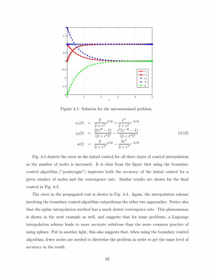
1.5
0.5
0
0-2
-1
-0.5
-1.5
x2
x1
λ2
λ1
u
1
1
2
2 3 4 5t
Figure 4-1: Solution for the unconstrained problem.
x1(t) =2
2 + e3e3/2t +
e3
2 + e3e−3/2t
x2(t) =2(e3t − 1)
(2 + e3)2− e6(e−3t − 1)
(2 + e3)2
u(t) =2
2 + e3e3/2t − 2e3
2 + e3e−3/2t
(4.12)
Fig. 4-2 depicts the error in the initial control for all three types of control interpolation
as the number of nodes is increased. It is clear from the figure that using the boundary
control algorithm (“pontryagin”) improves both the accuracy of the initial control for a
given number of nodes and the convergence rate. Similar results are shown for the final
control in Fig. 4-3.
The error in the propagated cost is shown in Fig. 4-4. Again, the interpolation scheme
involving the boundary control algorithm outperforms the other two approaches. Notice also
that the spline interpolation method has a much slower convergence rate. This phenomenon
is shown in the next example as well, and suggests that for some problems, a Lagrange
interpolation scheme leads to more accurate solutions than the more common practice of
using splines. Put in another light, this also suggests that, when using the boundary control
algorithm, fewer nodes are needed to discretize the problem in order to get the same level of
accuracy in the result.
82
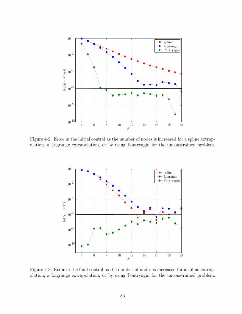
-2
4
0
-4
-6
-8
-106 8
10
10
10
10
10
1010 12 14 16 18 20
splineLagrangePontryagin
N
|u(τ
0)−
u∗ (
τ 0)|
Figure 4-2: Error in the initial control as the number of nodes is increased for a spline extrap-olation, a Lagrange extrapolation, or by using Pontryagin for the unconstrained problem.
-2
4
0
-4
-6
-8
-10
6 8
10
10
10
10
10
10
10 12 14 16 18 20
splineLagrangePontryagin
N
|u(τ
f)−
u∗ (
τ f)|
Figure 4-3: Error in the final control as the number of nodes is increased for a spline extrap-olation, a Lagrange extrapolation, or by using Pontryagin for the unconstrained problem.
83

-2
-1
-3
4
0
-4
-5
-6
-7
-86 8
10
10
10
10
10
10
10
10
1010 12 14 16 18 20
spline
Lagrange
Pontryagin
N
|J−
J∗ |
Figure 4-4: Error in the propagated cost as the number of nodes is increased for a spline ex-trapolation, a Lagrange extrapolation, or by using Pontryagin for the unconstrained problem.
4.2.2 Problem with a Path Constraint
Consider the following optimal control problem with three states and two controls:
minimize J = −x1(tf ) (4.13)
subject to the dynamic constraints
x1 = V u1
x2 = V u2
V = a − gu2
(4.14)
where
u21 + u2
2 = 1 (4.15)
84

and the boundary conditions
x1(0) = x2(0) = V (0) = 0
x2(tf ) = 0.1(4.16)
where tf = 2, g = 1, and a = 0.5g. Commonly known as the “max range” problem, where
x1 is the downrange direction, this problem was taken from Ref.22. The NLP solution is
compared to the boundary value problem solution using “bvp4c” in Matlab.77 The state
solution is shown in Fig. 4-5(a). The control solution is presented in Fig. 4-5(b).
x2
x1
0
0
0.1
0.2
0.2
0.3
0.4 0.6 0.8 1 1.2 1.4 1.6 1.8
-0.1
-0.2
-0.3
-0.4
(a) State Solution
1.5-1
2t
0
0
0.2
0.4
0.5
0.6
0.8
1
1
-0.2
-0.4
-0.6
-0.8
u1
u2
(b) Control Solution
Figure 4-5: Solution for the path constrained problem.
Since there are two elements of control in this problem, Figs. 4-8 and 4-9 depict the
error in the initial controls as the number of nodes is increased for all three types of control
interpolation. Again, the boundary control algorithm improves the initial control by several
orders of magnitude. Similar results are shown for the final controls in Figs. 4-10 and 4-11.
Recall in the boundary control algorithm presented in Section 4.1, the control path
constraint is enforced at the boundaries as well. If one were to simply extrapolate the
control using either splines or Lagrange polynomials, there would be no guarantee that
the path constraint would be satisfied, and therefore one could potentially end up with
an infeasible initial or final control. The boundary control algorithm guarantees a feasible
boundary control. Figs. 4-6 and 4-7 show that for small values of N , the path constraint is
indeed violated at the boundaries if “spline” or “Lagrange” extrapolation is used. However,
85

-2
0
0
-4
-6
-8
-10
-12
10
10
10
10
10
10
1010 20
spline
Lagrange
Pontryagin
5 15 25 30
Err
orm
agnit
ude
N
Figure 4-6: Error in the equality path constraint at τ0 as the number of nodes is increasedfor a spline extrapolation, a Lagrange extrapolation, or by using Pontryagin in the pathconstrained problem.
by using the “Pontryagin” approach presented in this chapter, the path constraint is always
satisfied at the boundaries, regardless of the number of nodes used.
The error in the propagated cost is shown in Fig. 4-12. As seen in Example 1, the
boundary control algorithm (“Pontryagin”) is the best performer, although for this example,
the improvement over the standard Lagrange interpolation is slight. However, the spline
interpolation method significantly underperforms, suggesting that splines are not the best
interpolation scheme to use for this type of problem.
[h]
4.2.3 Launch Vehicle Ascent Problem
The problem considered in this section is the guidance for a Delta III launch vehicle during
its ascent to orbit. The objective is to maneuver the launch vehicle from the ground to the
target orbit while maximizing the remaining fuel in the upper stage. This problem has been
rigorously studied and results are documented in Ref. 6.
86

-2
0
0
-4
-6
-8
-10
-12
-14
10
10
10
10
10
10
10
1010 20
splineLagrangePontryagin
5 15 25 30
Err
orm
agnit
ude
N
Figure 4-7: Error in the equality path constraint at τf as the number of nodes is increasedfor a spline extrapolation, a Lagrange extrapolation, or by using Pontryagin in the pathconstrained problem.
0
0
-5
-10
-15
10
10
10
1010 20
spline
Lagrange
Pontryagin
5 15 25 30
Err
orm
agnit
ude
N
Figure 4-8: Error in the initial control, u1(t0), as the number of nodes is increased for a splineextrapolation, a Lagrange extrapolation, or by using Pontryagin in the path constrainedproblem.
87

0
0
-5
-10
-15
10
10
10
1010 20
splineLagrangePontryagin
5 15 25 30
Err
orm
agnit
ude
N
Figure 4-9: Error in the initial control, u2(t0), as the number of nodes is increased for a splineextrapolation, a Lagrange extrapolation, or by using Pontryagin in the path constrainedproblem.
Vehicle Properties
The Delta III expendable launch vehicle has two stages along with nine strap-on solid rocket
boosters. The flight of the vehicle can be divided into four distinct phases. The first phase
begins with the rocket at rest on the ground and at time t0, the main engine and six of
the nine solid boosters ignite. When the boosters are depleted at time t1, their remaining
dry mass is ejected. The final three boosters are ignited, and along with the main engine,
represent the thrust for phase two of the flight. These boosters are then ejected once their
fuel is exhausted at time t2, and the main engine alone creates the thrust for phase three.
The fourth phase begins when the main engine fuel has been exhausted (MECO) and the
dry mass associated with the main engine is ejected at time t3. The thrust during phase
four is from a second stage, which burns until the target orbit has been reached (SECO) at
time t4, thus completing the trajectory. The specific characteristics of these rocket motors
can be seen in Table 4.1. Note that the solid boosters and main engine burn for their entire
duration (meaning t1, t2, and t3 are fixed), while the second stage engine is shut off when
88
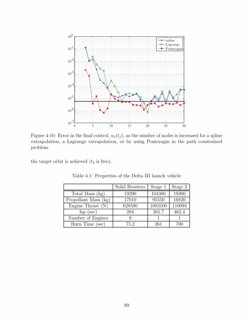
-2
-1
-3
0
0
-4
-5
-6
-7
10
10
10
10
10
10
10
1010 20
splineLagrangePontryagin
5 15 25 30
Figure 4-10: Error in the final control, u1(tf), as the number of nodes is increased for a splineextrapolation, a Lagrange extrapolation, or by using Pontryagin in the path constrainedproblem.
the target orbit is achieved (t4 is free).
Table 4.1: Properties of the Delta III launch vehicle
Solid Boosters Stage 1 Stage 2
Total Mass (kg) 19290 104380 19300Propellant Mass (kg) 17010 95550 16820Engine Thrust (N) 628500 1083100 110094
Isp (sec) 284 301.7 462.4Number of Engines 9 1 1Burn Time (sec) 75.2 261 700
89

-2
-1
-3
0
-4
-5
-6
-7
10
10
10
10
10
10
1010 20
splineLagrangePontryagin
5 15 25 30
Err
orm
agnit
ude
N
Figure 4-11: Error in the final control, u2(tf), as the number of nodes is increased for a splineextrapolation, a Lagrange extrapolation, or by using Pontryagin in the path constrainedproblem.
Dynamic Model
The equations of motion for a non-lifting point mass in flight over a spherical rotating planet
are expressed in Cartesian Earth centered inertial (ECI) coordinates as
r = v
v = − µ
‖r‖3r +
T
mu +
D
m
m = − T
g0Isp
(4.17)
where r(t) =[
x(t) y(t) z(t)]T
is the position, v =[
vx(t) vy(t) vz(t)]T
is the Carte-
sian ECI velocity, µ is the gravitational parameter, T is the vacuum thrust, m is the mass,
g0 is the acceleration due to gravity at sea level, Isp is the specific impulse of the engine,
u =[
ux uy uz
]T
is the thrust direction, and D =[
Dx Dy Dz
]T
is the drag force.
The drag force is defined as
D = −1
2CDArefρ‖vrel‖vrel (4.18)
90
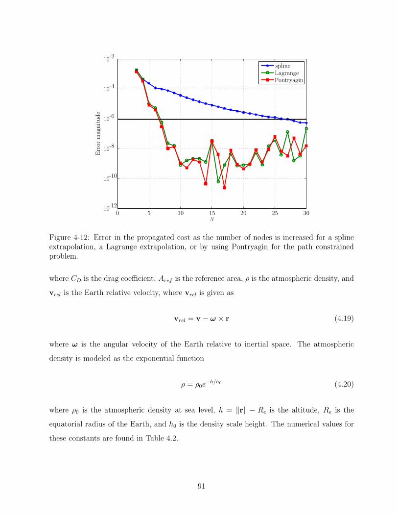
-2
0
-4
-6
-8
-10
-12
10
10
10
10
10
1010 20
splineLagrangePontryagin
5 15 25 30
Err
orm
agnit
ude
N
Figure 4-12: Error in the propagated cost as the number of nodes is increased for a splineextrapolation, a Lagrange extrapolation, or by using Pontryagin for the path constrainedproblem.
where CD is the drag coefficient, Aref is the reference area, ρ is the atmospheric density, and
vrel is the Earth relative velocity, where vrel is given as
vrel = v − ω × r (4.19)
where ω is the angular velocity of the Earth relative to inertial space. The atmospheric
density is modeled as the exponential function
ρ = ρ0e−h/h0 (4.20)
where ρ0 is the atmospheric density at sea level, h = ‖r‖ − Re is the altitude, Re is the
equatorial radius of the Earth, and h0 is the density scale height. The numerical values for
these constants are found in Table 4.2.
91

Table 4.2: Constants used in the Delta III launch vehicle problem
Constant Value
Payload Mass (kg) 4164Aref (m2) 4π
Cd 0.5ρ0 (kg/m3) 1.225h0 (km) 7.2t1 (s) 75.2t2 (s) 150.4t3 (s) 261
Re (km) 6378.14VE (km/s) 7.905
Constraints
The launch vehicle starts on the ground at rest (relative to the Earth) at time t0, so that
the ECI initial conditions are
r(t0) = r0 =[
5605.2 0 3043.4]T
km
v(t0) = v0 =[
0 0.4076 0]T
km/s
m(t0) = m0 = 301454 kg
(4.21)
which corresponds to the Cape Canaveral launch site. The terminal constraints define the
target geosynchronous transfer orbit (GTO), which is defined in orbital elements as
af = 24361.14 km,
ef = 0.7308,
if = 28.5 deg,
Ωf = 269.8 deg,
ωf = 130.5 deg
(4.22)
The orbital elements, a, e, i, Ω, and ω represent the semi-major axis, eccentricity, inclina-
tion, right ascension of the ascending node (RAAN), and argument of perigee, respectively.
Note that the true anomaly, ν, is left undefined since the exact location within the orbit is
92
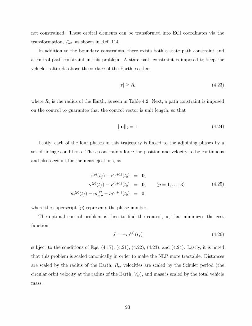
not constrained. These orbital elements can be transformed into ECI coordinates via the
transformation, To2c as shown in Ref. 114.
In addition to the boundary constraints, there exists both a state path constraint and
a control path constraint in this problem. A state path constraint is imposed to keep the
vehicle’s altitude above the surface of the Earth, so that
|r| ≥ Re (4.23)
where Re is the radius of the Earth, as seen in Table 4.2. Next, a path constraint is imposed
on the control to guarantee that the control vector is unit length, so that
||u||2 = 1 (4.24)
Lastly, each of the four phases in this trajectory is linked to the adjoining phases by a
set of linkage conditions. These constraints force the position and velocity to be continuous
and also account for the mass ejections, as
r(p)(tf) − r(p+1)(t0) = 0,
v(p)(tf ) − v(p+1)(t0) = 0, (p = 1, . . . , 3)
m(p)(tf) − m(p)dry − m(p+1)(t0) = 0
(4.25)
where the superscript (p) represents the phase number.
The optimal control problem is then to find the control, u, that minimizes the cost
function
J = −m(4)(tf) (4.26)
subject to the conditions of Eqs. (4.17), (4.21), (4.22), (4.23), and (4.24). Lastly, it is noted
that this problem is scaled canonically in order to make the NLP more tractable. Distances
are scaled by the radius of the Earth, Re, velocities are scaled by the Schuler period (the
circular orbit velocity at the radius of the Earth, VE), and mass is scaled by the total vehicle
mass.
93
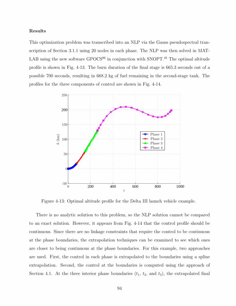
Results
This optimization problem was transcribed into an NLP via the Gauss pseudospectral tran-
scription of Section 3.1.1 using 20 nodes in each phase. The NLP was then solved in MAT-
LAB using the new software GPOCS86 in conjunction with SNOPT.45 The optimal altitude
profile is shown in Fig. 4-13. The burn duration of the final stage is 665.3 seconds out of a
possible 700 seconds, resulting in 668.2 kg of fuel remaining in the second-stage tank. The
profiles for the three components of control are shown in Fig. 4-14.
200 400 600 800 1000
200
0
0-50
50
100
150
250
h(k
m)
t
Phase 1Phase 2Phase 3Phase 4
Figure 4-13: Optimal altitude profile for the Delta III launch vehicle example.
There is no analytic solution to this problem, so the NLP solution cannot be compared
to an exact solution. However, it appears from Fig. 4-14 that the control profile should be
continuous. Since there are no linkage constraints that require the control to be continuous
at the phase boundaries, the extrapolation techniques can be examined to see which ones
are closer to being continuous at the phase boundaries. For this example, two approaches
are used. First, the control in each phase is extrapolated to the boundaries using a spline
extrapolation. Second, the control at the boundaries is computed using the approach of
Section 4.1. At the three interior phase boundaries (t1, t2, and t3), the extrapolated final
94

0
0
0.2
0.4
0.6
0.8
1
-0.2
-0.4
-0.6
-0.8
t
ux
uy
uz
200 400 600 800 1000
ui,
i=
1,2,
3
Figure 4-14: Profile of the three components of the optimal control for the Delta III launchvehicle example.
control from one phase is compared to the extrapolated initial control of the next phase, or
|ui(tk)− − ui(tk)
+|, where ui, (i = 1, 2, 3) are the three components of control and tk, (k =
1, 2, 3) are the three phase interfaces. The difference in extrapolated controls are shown for
the spline extrapolation in Fig. 4-15 versus the number of nodes per phase. A similar graph
is shown for the Pontryagin extrapolated controls in Fig. 4-16. In the spline extrapolation,
the difference between the extrapolated controls is roughly 10−3 when using 10 nodes, and
gradually becomes more accurate as the number of nodes increases. Using Pontryagin, on
the other hand, produces extremely similar boundary controls (∼ 10−6) for small numbers of
nodes, which is a significant improvement over the spline approach. The results of Fig. 4-16
hover around the optimality tolerance of 10−6 for all the simulations tested.
4.3 Summary
This chapter described a method to obtain more accurate information about the control at
the boundary through post-processing. A post-optimality computation is performed where
95

|ui(t
k)− −
ui(t
k)+|
(t )
(t )
(t )
(t )
(t )
(t )
(t )
(t )
(t )
-2
-3
u
u
u
u
u
u
u
u
u
2
2
22
2
2
33
3
3
3
3
-4
-5
-6
-7
-8
10
10
10
10
10
10
1010 20
N
1
1
1
1
11
15 25 30 35 40 45
Figure 4-15: The difference in spline-extrapolated control, |ui(tk)− − ui(tk)
+|, at all threeinterior phase interfaces in the launch vehicle example. Some differences are significantlygreater than the optimality tolerance of 1e − 6.
|ui(t
k)− −
ui(t
k)+|
(t )
(t )
(t )
(t )
(t )
(t )
(t )
(t )
(t )
-2
-3
u
u
u
u
u
u
u
u
u
2
2
22
2
2
33
3
3
3
3-4
-5
-6
-7
-8
-9
10
10
10
10
10
10
10
1010 20
N
1
1
1
1
11
15 25 30 35 40 45
Figure 4-16: The difference in Pontryagin-extrapolated control, |ui(tk)− − ui(tk)
+|, at allthree interior phase interfaces in the launch vehicle example. Almost all differences lie belowthe optimality tolerance of 1e − 6.
96

the Pontryagin minimum principle is applied at the boundary points in order to obtain a more
accurate control approximation at the initial and final times. The results show signifcant
improvement in simulation when compared with a control approximation that uses various
extrapolation techniques to compute the boundary control.
97

[This page intentionally left blank.]

Chapter 5
Local versus Global Orthogonal
Collocation Methods
Orthogonal collocation methods are traditionally global in nature, meaning that a global
interpolating polynomial spans the entire problem interval. However, orthogonal collocation
methods have been used locally,27,72 meaning the problem interval is divided into segments
and a “global” interpolating polynomial spans the width of each segment. The segments are
then connected by various linkage conditions, similar to the concept of phases presented in
Chapter 3. The conceptual difference between phases and segments are that phase interfaces
usually represent a physical event (such as a mass drop in a launch vehicle problem), whereas
segment interfaces are simply a construct of the numerical approximation procedure, and
tend to be more numerous. Furthermore, phases may occur in parallel, while segments are
sequential in the independent variable (as seen in Chapter 7).
This chapter compares the theory and implementation of a global and local approach
for the Gauss pseudospectral method. Proponents of the global approach tout the “spectral
accuracy” (see Chapter 2) of the method for smooth problems, while proponents of the local
approach claim the benefits of “local support”. These two approaches are compared on two
example problems. The first example is a smooth problem with nonlinear dynamics and a
quadratic cost, while the second example is a “bang-bang” problem that is discontinuous in
the control. Each method is evaluated on accuracy of the NLP solution, convergence rate,
and computational efficiency.
99

5.1 Local GPM Approach: Segments
First, the description of the Gauss pseudospectral transcription of Chapter 3 is slightly
modified to reflect the partitioning of the optimal control problem into segments. This
local application of the GPM is a similar approach to that found in Refs. 26, 71, 104. The
continuous Bolza problem of Eqs. (2.7)–(2.10) is transcribed to a nonlinear programming
problem using the local Gauss pseudospectral method as follows. First, the original time
interval I = [t0, tf ] is divided into S sub-intervals (or segments) Is, (s = 1, . . . , S) such that
Is = [ts−1, ts] and
S⋂
s=1
Is = ∅
S⋃
s=1
Is = I
where ∅ is the empty set. Within each sub-interval, the time, t(s), is transformed to the
interval [−1, 1] via the affine transformation
τ (s) =2t(s)
ts − ts−1
− ts + ts−1
ts − ts−1
(5.1)
where τ (s) ∈ [−1, 1] and denotes the transformed time in Is. Each sub-interval Is, is dis-
cretized according to the GPM. For example, the state is approximated using a basis of N +1
Lagrange interpolating polynomials, Li(τ), (i = 0, . . . , K), as in Eq. (3.1):
x(s)(τ) ≈ X(s)(τ) =
K∑
i=0
X(s)(τi)Li(τ) (5.2)
where K is the number of Legendre-Gauss points. The resulting NLP is as follows: Minimize
J = Φ(X(1)0 , t
(1)0 ,X
(S)f , t
(S)f ) +
S∑
s=1
[
t(s)f − t
(s)0
2
K∑
k=1
w(s)k g(X
(s)k ,U
(s)k , τ
(s)k ; ts−1, ts)
]
(5.3)
100

subject to the dynamic constraint
K∑
i=0
D(s)ki X
(s)i −
t(s)f − t
(s)0
2f(X
(s)k ,U
(s)k , τ
(s)k ; ts−1, ts) = 0,
(k = 1, . . . , K), (s = 1, . . . , S)
(5.4)
and the Gauss quadrature
X(s)f ≡ X
(s)0 +
t(s)f − t
(s)0
2
K∑
k=1
w(s)k f(X
(s)k ,U
(s)k , τ
(s)k ; ts−1, ts), (s = 1, . . . , S) (5.5)
where X(s)k ≡ X(τ
(s)k ) ∈ R
n and U(s)k ≡ U(τ
(s)k ) ∈ R
m. Next, the boundary constraint of
Eq. (2.9) is expressed as
φ(X(1)0 , t
(1)0 ,X
(S)f , t
(S)f ) = 0 (5.6)
Furthermore, the path constraint of Eq. (2.10) is evaluated at the LG points in each segment
as
C(X(s)k ,U
(s)k , τ
(s)k ; ts−1, ts) ≤ 0 (k = 1, . . . , K), (s = 1, . . . , S) (5.7)
Lastly, the state can be constrained to be continuous across segment boundaries by including
the following linkage conditions:
L(s+1)(s) (X
(s)f , t
(s)f ,X
(s+1)0 , t
(s+1)0 ) = 0, (s = 1, . . . , S − 1) (5.8)
The cost function of Eq. (5.3) and the algebraic constraints of Eqs. (5.4), (5.5), (5.6), (5.7),
and (5.8) define an NLP whose solution is an approximate solution to the continuous Bolza
problem.
In the case where one sub-interval is used (i.e., S = 1), the GPM is employed as a global
collocation method. Conversely, in this analysis it is assumed that any case where S ≫ 1, to
be a local application of the method (although, strictly speaking, this is untrue). In the latter
case, the sub-intervals are connected via linkage conditions on the state, the independent
variable, and, possibly, the control. The analysis that follows compares the GPM in both
global collocation (i.e., S = 1) and local collocation (i.e., S ≫ 1) for a given number of total
101

discretization points.
5.2 Global and Local Applications of the GPM
In this comparison, the Gauss pseudospectral method is applied as both a global and a
local collocation method on two examples. As a global collocation method, the number of
segments is set to unity (i.e., S = 1) and the accuracy is assessed as a function of the number
of collocation points, N . As a local collocation method, the number of collocation points in
a given sub-interval is fixed and the number of sub-intervals is varied. In the local approach,
five nodes (three LG points plus two boundary points) are chosen for each sub-interval and
the width of each sub-interval is constrained to be equal. Fig. 5-1 depicts the distribution
of nodes and collocation points for both the global and local approaches using a total of 20
discretization points. Recall from Chapter 2 that the LG points are more dense near the
endpoints than in the middle, which is readily apparent in Fig. 5-1. It is emphasized that, for
both approaches, once the number of LG points per interval is determined, the location of
each point inside the interval is immediately fixed. All examples in this chapter were solved
using the TOMLABR© version59 of the sparse NLP solver SNOPT45 with default tolerances
and comparable initial guesses for both the local and global approaches. A Pentium 4,
3.2 GHz desktop computer was used for all computations and any documented computation
times are in reference to this machine.
5.2.1 Modified Hicks-Ray Reactor Problem
Consider the Hicks-Ray reactor problem104 where it is desired to minimize the quadratic cost
functional∫ 10
0
[
a1(C(t) − C)2 + a2(T (t) − T )2 + a3(U(t) − U)2]
dt (5.9)
102

global nodesglobal collocation pointslocal nodeslocal collocation points
segment 1 segment 2 segment 3 segment 4
8 100
2
2 4 6
1
t)
Figure 5-1: Distribution of nodes and collocation points for both the global and local ap-proaches (N = 20).
subject to the nonlinear dynamic constraints
C(t) =1 − C(t)
θ− k10C(t)e−t/T (t) (5.10)
T (t) =yf − T (t)
θ+ k10C(t)e−t/T (t) (5.11)
−α(T (t) − yc)U(t) (5.12)
and the initial conditions
C(0) = 0.1367
T (0) = 0.7293(5.13)
The two states are denoted by C(t) and T (t), the control is denoted by U(t), and all other
parameters are constants. This problem has no analytic solution, however, this analysis
compares the NLP solutions to a highly accurate extremal solution of the Hamiltonian
boundary-value problem (HBVP) associated with Eqs. (5.9)–(5.13). This HBVP solution
was found using the MATLAB boundary-value problem solver BVP4C77 and is shown in
Fig. 5-2. Finally, it is noted that the traditional form of this example includes the (active)
103

path constraint U(t) ≥ 0. However, due to the increased difficulty in accurately solving a
path-constrained HBVP and the fact that this is simply an illustrative example, the path
constraint was omitted for this analysis.
The results obtained by solving the Hicks-Ray reactor problem using GPM as both a
global and a local collocation method are shown in Figs. 5-3 and 5-4, respectively. The
“error” in these figures represent the maximum absolute error between the NLP state and
the HBVP state across the discretized trajectory for a given number of nodes, N . Fig. 5-3
shows the error for the global approach as the number of nodes increases. It is seen from
Fig. 5-3 that the error decreases at a spectral rate43 as N increases and attains a minimum
just below the feasibility tolerance of 10−6 for discretizations with at least 21 nodes. This
rapid convergence is typical for pseudospectral methods and is one of the primary motivations
for using a global approach. As for the local approach, Fig. 5-4 shows the error in the state
as a function of the number of segments where five nodes (three LG points) were used per
segment. The state errors using local collocation converge at a much slower rate than seen
in the global approach. Notice that the data shown for the global approach end at 30
nodes while the data for the local approach extend to 25 segments, or 125 total nodes. For
comparison, the vertical line in Fig. 5-4 represents the largest number of nodes used in the
global scenario. Thus for 30 total nodes, the global method has an accuracy better than
10−6 (Fig. 5-3), while the local method produces an accuracy of ∼ 10−3 (Fig. 5-4). Often
in practice, it is desirable to know how many nodes are required to achieve a certain level
of accuracy. The data in this example show that to achieve an accuracy of 10−5, one would
need 16 nodes in the global approach and more than 125 total nodes in the local approach.
Although the global method outperforms the local method in accuracy, one must also
consider the computational efficiency between the two approaches. First, it is noted that,
for the same number of nodes, the global method results in a much more dense constraint
Jacobian as compared to the local method since the collocation equations are a function of
the state and control across the entire interval in the global method. However, as seen from
Fig. 5-4, for a certain required accuracy, the local approach needs many more collocation
points as compared to the global approach. This results in a much larger, albeit sparser
Jacobian for the local approach. Table 5.1 summarizes the performance of each method
104

for a desired accuracy. Specifically, Table 5.1 shows that, for a desired accuracy, the local
method requires significantly more computational effort as compared to the global approach
both in terms of CPU time and major iterations of the NLP solver. Table 5.1 also shows
that the larger, sparser Jacobian of the local approach results in a higher number of nonzero
elements than the smaller, more dense counterpart in the global approach, which is the
likely contributer to the higher computational expense. This result is not intuitive, as one
might expect the sparse NLP solver to perform faster on the large, sparse approach. For this
example, the extremely high accuracy of global polynomials outweighs the more numerous
but relatively inexpensive computations of the local approach.
Table 5.1: Computational expense for both the global and local approach in the Hicks-Rayreactor problem
GlobalApproach
Accuracy Nodes Non- Jacobian CPU Major MinorRequired Zeros Density (%) Time (s) Iterations Iterations
1e-3 10 248 46 1.343 29 451e-4 12 348 44 1.234 31 551e-5 16 596 41 5.047 113 1441e-6 21 996 40 6.531 115 171
LocalApproach
Accuracy Nodes Non- Jacobian CPU Major MinorRequired Zeros Density (%) Time (s) Iterations Iterations
1e-3 35 512 6.6 8.890 43 1001e-4 80 1178 2.8 49.86 56 1741e-5 165 2436 1.4 148.3 44 285
5.2.2 Problem with Discontinuous Control
In this problem, it is desired to minimize the cost functional
J = tf (5.14)
105

7 90.05
0.15
7 90.7
0.75
7 9−1000
8
8
8
10
10
10
0.1
1000
0
0
0
0
2
2
2
3
3
3
4
4
4
5
5
5
6
6
6
0.8
1
1
1C
TU
C
T
U
t
Figure 5-2: BVP solution to the Hicks-Ray reactor problem.
subject to the dynamic constraints
x1(t) = x2(t)
x2(t) = u(t)(5.15)
the boundary conditions
x1(0) = x10 ; x2(0) = x20
x1(tf) = 0 ; x2(tf ) = 0(5.16)
and the inequality control constraint
|u(t)| ≤ 1 (5.17)
The key difference between this example and the previous example is that, for a wide variety
of initial conditions, the optimal control for this problem is “bang-bang”, i.e., it switches
from either its maximum value to its minimum value (or vice-versa) at a time tb (where
106

10
10
10
10
10
10
1010 2015 25 30
-7
-6
-5
-4
-3
-2
-1
5
Costate
Err
or
N
C Error
T Error
Figure 5-3: Convergence of Hicks-Ray Problem via global approach as a function of thenumber of nodes, N .
0 < tb < tf ). Because of the discontinuity in the optimal control, it would appear at first
glance that a global approximation would be much less accurate than a local approximation.
However, the two methods are surprisingly comparable in their solution accuracy for this
problem.
Example 2 Solved without Knowledge of Discontinuity
The discontinuity in the control can drastically affect the accuracy of each approach depend-
ing on where the discontinuity is located. In order to fully assess the accuracy of solutions,
two different sets of initial conditions are considered. The first set of initial conditions is as
follows:
x10 = 3, x20 = 2 (5.18)
For the initial conditions of Eq. (5.18) the optimal switch time of the control is tb ≈ 4.2361,
which is designed to lie on the interior of a segment in both the global and local approaches,
107

30 nodes
10
10
10
10
10
10
1010 2015 25
-7
-6
-5
-4
-3
-2
-1
0 5
Costate
Err
or
S
C Error
T Error
Figure 5-4: Convergence of Hicks-Ray problem via local approach as a function of the numberof segments, S (5 nodes per segment).
as opposed to on a segment boundary. Figs. 5-5 and 5-6 show the solutions for these initial
conditions which employ 40 nodes for the global GPM and 8 equally-spaced segments with
5 nodes per segment (40 nodes total) for the local GPM. Furthermore, Figs. 5-7 and 5-8
show the errors in the state (x1 and x2) and costate (λ1 and λ2) obtained from the global
and local GPM methods, respectively. Naturally, for both approaches the largest error in
the state occurs at the switch time. Note that the error in these figures is the absolute
difference between the NLP solution and exact analytic solution. Figs. 5-5–5-8 show clearly
that the results from both approaches are strikingly similar, and that the global approach is
slightly more accurate. Critics of global methods claim that by shifting the nodes towards
the boundaries, the sparsity of nodes in the middle of the trajectory degrades the accuracy
of the approximation. However, despite a reduced density in the center of the interval, the
maximum error is actually smaller with the global approach.
108

7
GPM x1GPM x2Exact x1Exact x2
7
7
-5
-2
-1
0
0
0
0
0
0
2
2
2
2
3
3
3
4
4
4
5
5
5
5
6
6
6
1
1
1
1
t
GPM u
Exact u
GPM λ1
GPM λ2
Exact λ1
Exact λ2
ux
λ
Figure 5-5: Solution to double integrator problem for initial conditions of Eq. (5.18) usingglobal LG collocation with 40 nodes.
Example 2 Solved with Knowledge of Discontinuity
It is important to note that both the global and local applications of the GPM assumed no
prior knowledge of the control switching time, tb. As is often the case, even if a disconti-
nuity in the solution is expected, the exact location of the discontinuity may be unknown.
Therefore in general, the switch time will not coincide with a segment interface when using
the local approach. However, one of the benefits of the local approach is that, if a switching
time is known, a segment interface can be located to coincide with this switch time. Yet this
concept can be applied to the global approach as well. The global approach then becomes
a semi-global approach where the number of segments is one greater than the number of
known discontinuities. This semi-global approach has been developed for different classes of
optimal control problems using the Legendre pseudospectral method38,85, 92, 95 and the Gauss
pseudospectral method.66–68
In order to assess how a priori knowledge of the discontinuity can improve accuracy in
109

7
7
7
-5
-2
-1
-1
0
0
0
0
0
0
2
2
2
2
3
3
3
4
4
4
5
5
5
5
6
6
6
1
1
1
1
1
t
GPM x1
GPM x2
GPM u
Exact u
GPM λ1
GPM λ2
Exact x1
Exact x2
Exact λ1
Exact λ2
ux
λ
Figure 5-6: Solution to double integrator problem for initial conditions of Eq. (5.18) usinglocal LG collocation with 8 segments of 5 nodes each.
both the global and local approaches, consider the following initial conditions:
x10 = −1 x20 = 2 (5.19)
The initial conditions of Eq. (5.19) has the interesting feature that the switch time in the
control is exactly tb = 3 and the optimal final time is t∗f = 4. Consequently, when a local
approach is employed with 8 equally spaced segments [i.e., the same number of segments
used with Eq. (5.18)], the switch time of the control lies at the boundary between the sixth
and seventh segments.
Using the initial conditions of Eq. (5.19), the GPM is employed in the following two
ways. First, the semi-global GPM is employed using two segments of 20 nodes each, where
the segment interface occurs at t = 3. The local GPM is employed as before with 8 segments
and 5 nodes per segment. The results of these two cases is shown in Figs. 5-9– 5-12. The
accuracy of both methods is improved dramatically. Comparing Figs. 5-11 and 5-12 it is
seen again that for all relevant quantities, the error using the local GPM is slightly larger
110

7
0.01
0.02
0.03
0.04
0.05
0.06
00 2 3 4 5 61
t
Mag
nit
ude
Err
or
x1 Error
x2 Error
λ1 Error
λ2 Error
Figure 5-7: Error in state and costate for the double integrator problem using initial condi-tions of Eq. (5.18) and global LG collocation with 40 nodes.
than the corresponding error using global GPM. Although it isn’t clear from Figs. 5-11 and
5-12 , the state is accurate to within the NLP tolerances due to the fact that the solution
is a piecewise polynomial expression and can be approximated exactly with at least three
collocaion points per phase.
5.3 Summary
A comparison was made between a global and a local implementation of the Gauss pseu-
dospectral method. The purpose of the comparison was to determine the accuracy and
computational efficiency of each approach. Employing the GPM as a local method, the
number of collocation points within each segment was held fixed at a small number (e.g.,
three collocation points) while the number of segments was varied. In global collocation
form, a single segment was used and the number of collocation points was varied. Analysis
of the examples in this chapter suggests that for smooth problems, global collocation is sig-
111

7
0.01
0.02
0.03
0.04
0.05
0.06
00 2 3 4 5 61
t
Mag
nit
ude
Err
or
x1 Error
x2 Error
λ1 Error
λ2 Error
Figure 5-8: Error in state and costate for the double integrator problem using initial condi-tions of Eq. (5.18) and local LG collocation with 8 segments of 5 nodes each.
nificantly more accurate than local collocation for a given number of total collocation points.
For nonsmooth problems, the accuracies of global and local collocation methods were found
to be comparable, and if the discontinuities are known a priori, a semi-global approach is
the most accurate approach. Furthermore it was found that, for a desired accuracy, the
global approach was computationally more efficient for smooth problems . These claims
were supported by two example problems which had features that might lead one to prefer
the use of a local method.
112

-2
-2
-1
0
0
0
0
0
0
0.5
0.5
0.5
1.5
1.5
1.5
2
2
2
2
2
2.5
2.5
2.5
3
3
3
3.5
3.5
3.5
4
4
4
4
1
1
1
1
t
GPM x1
GPM x2
GPM u
Exact u
GPM λ1
GPM λ2
Exact λ1
Exact λ1
Exact λ2
Exact λ2
ux
λ
Figure 5-9: Solution to the double integrator problem with the initial conditions of Eq. (5.19)and semi-global LG collocation with two segments of 20 nodes each.
-2
-1
-1
-1
-0.5
0
0
0
0
0
0
0.5
0.5
0.5
0.5
1.5
1.5
1.5
2
2
2
2
2
2.5
2.5
2.5
3
3
3
3
3.5
3.5
3.5
4
4
4
1
1
1
1
1
1
t
GPM x1
GPM x2
GPM u
Exact u
GPM λ1
GPM λ2
Exact x1
Exact x2
Exact λ1
Exact λ2
ux
λ
Figure 5-10: Solution to the double integrator problem with the initial conditions ofEq. (5.19) and local LG collocation.
113
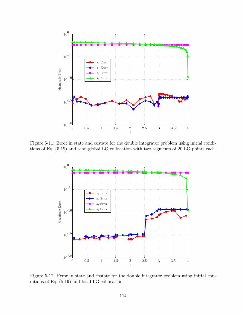
−20
-10
-15
10
10
10
10
10
-5
0
0 0.5 1.5 2 2.5 3 3.5 41t
Mag
nit
ude
Err
orx1 Error
x2 Error
λ1 Error
λ2 Error
Figure 5-11: Error in state and costate for the double integrator problem using initial condi-tions of Eq. (5.19) and semi-global LG collocation with two segments of 20 LG points each.
−20
-10
-15
10
10
10
10
10
-5
0
0 0.5 1.5 2 2.5 3 3.5 41t
Mag
nit
ude
Err
or
x1 Error
x2 Error
λ1 Error
λ2 Error
Figure 5-12: Error in state and costate for the double integrator problem using initial con-ditions of Eq. (5.19) and local LG collocation.
114

Chapter 6
Comparison between Three
Pseudospectral Methods
This chapter analyzes the performance of three pseudospectral methods: the Gauss,8 Radau,72
and Legendre33 pseudospectral methods. All three approaches are global in nature and imple-
ment orthogonal collocation based on Legendre polynomials. The key distinctions between
these methods lie in the choice of both the discretization points and collocation points. This
chapter introduces these differences, discusses the mathematical implications of each set
of points, and numerically compares the three methods with respect to the accuracy and
convergence rates of the resulting NLP state, control, and costate solution.
6.1 Continuous Mayer Problem
Without loss of generality, consider the following optimal control problem in Mayer form.
Determine the control, u(τ) ∈ Rm, that minimizes the cost functional
J = Φ(x(τf )) (6.1)
subject to the constraints
dx
dτ=
tf − t02
f(x(τ),u(τ)) ∈ Rn (6.2)
115
φ(x(τ0),x(τf )) = 0 ∈ Rq (6.3)
The optimal control problem of Eqs. (6.1)–(6.3) is referred to as the continuous Mayer
problem. It is noted that, in order to simplify the analysis and provide a clear comparison, this
chapter considers optimal control problems with fixed terminal times and without algebraic
path constraints. As in Chapter 2, the time interval τ ∈ [−1, 1] can be transformed to the
arbitrary time interval t ∈ [t0, tf ] via the affine transformation of Eq. (2.6).
6.2 First-Order Necessary Conditions of Continuous
Mayer Problem
Following a similar procedure to the continuous Bolza problem of Chapter 2, the indirect
approach to solving the continuous Mayer problem of Eqs. (6.1)–(6.3) is to apply the calculus
of variations to obtain first-order necessary conditions for optimality.73 These variational
conditions are derived using the Hamiltonian, H, defined for the Mayer problem as
H(x, λ,u) = λT f(x,u) (6.4)
where λ(τ) ∈ Rn is the costate. Note that, for brevity, the explicit dependence of the state,
control, and costate on τ has been dropped. Assuming that the optimal control lies within
the feasible control set, the continuous-time first-order optimality conditions are
dx
dτ
T
=tf − t0
2fT (x,u) =
tf − t02
∂H∂λ
dλ
dτ
T
= −tf − t02
λT ∂f
∂x= −tf − t0
2
∂H∂x
0T = λT ∂f
∂u=
∂H∂u
φ(x(τ0),x(τf )) = 0
λ(τ0)T = νT ∂φ
∂x(τ0), λ(τf )
T =∂Φ
∂x(τf )− νT ∂φ
∂x(τf)
(6.5)
116

where ν ∈ Rq is Lagrange multiplier associated with the boundary condition φ. The opti-
mality conditions of Eq. (6.5) define a Hamiltonian boundary value problem (HBVP).
6.3 Descriptions of the Pseudospectral Methods
The three pseudospectral methods in this comparison approximate the state using a finite
basis of global polynomials, which are created by first discretizing the problem into N nodes
along the trajectory (described in Chapter 2). However, the points within the node set, N ,
are unique to each method, along with the choice of basis polynomials. These differences
are explained in detail in this section. Furthermore, all pseudospectral methods transcribe
the dynamic equations into algebraic conditions, which are evaluated at a set of collocation
points, K. This set of collocation points is also unique to each method and may or may not
be the same as the node set. The locations of nodes and collocation points, as well as the
choice of basis functions are key features that distinguish these methods from each other.
There are many different types of pseudospectral methods, but this comparison is limited
to three methods: the Legendre, Radau, and Gauss pseudospectral methods, since these are
the three methods with published costate approximation procedures. The Gauss method has
already been described in detail in Chapter 3, so this chapter provides only a brief overview.
The Legendre and Radau direct transcription methods are described here in more detail and
the key differences between the methods are highlighted. It is noted that the indexing in this
section may be slightly different than the indexing contained in the references. This is done
in order to create some commonality between the three methods in terms of their indices,
and to create NLPs that are equivalent in size. Therefore, in all methods, N represents the
total number of discretization points (nodes) used in the NLP, which is kept the same among
all methods for the numerical comparisons in this chapter. Moreover, in general, the index j
is used to represent the j-th node, while the index k is used to represent the k-th collocation
point.
117

6.3.1 Legendre Pseudospectral Method (LPM)
The Legendre pseudospectral method (LPM), like all pseudospectral methods, is based on
approximating the state using a finite set of interpolating polynomials. The state is ap-
proximated using a basis of N Lagrange interpolating polynomials, Li(τ) (i = 1, . . . , N), as
defined in Eq. (2.23).
x(τ) ≈ X(τ) =N∑
i=1
Li(τ)X(τi) (6.6)
In the LPM, the location of N nodes are described by the Legendre-Gauss-Lobatto (LGL)
points on the interval τ ∈ [−1, 1] which were defined in Chapter 2. Note that the endpoints
−1 and 1 are included in the state approximation.
Next, all pseudospectral methods transcribe the dynamic equations by collocating the
derivative of this state approximation with the vector field, f(x,u), at a set of points along
the interval. Let us assume there are K collocation points. In the LPM, the LGL points are
both the nodes and the collocation points, meaning the two sets are equivalent (N = K).
Naturally, the number of points in both sets is the same as well (N = K). Mathematically,
the derivative of the state approximation at the k-th LGL point, τk, is
x(τk) ≈ X(τk) =N∑
i=1
Li(τk)X(τi) =N∑
i=1
DkiX(τk), (k = 1, . . . , K) (6.7)
where the differentiation matrix, D ∈ RK×N , is defined as
Dki =
PN−1(τk)
PN−1(τi)1
τk−τi, if k 6= i
− (N−1)N4
, if k = i = 1
(N−1)N4
, if k = i = N
0, otherwise
(6.8)
The continuous dynamics of Eq. (6.2) are then transcribed into the following set of K alge-
braic equations via collocation described in Chapter 2 by Eq. (2.33):
N∑
i=1
DkiX(τi) −tf − t0
2f(X(τk),U(τk)) = 0, (k = 1, . . . , K) (6.9)
118

The approximated control, U(τ), is defined in a similar manner as the state:
u(τ) ≈ U(τ) =N∑
i=1
Li(τ)U(τi) (6.10)
where τi, i = 1, . . . , N are the LGL nodes. Again, it is emphasized that in the LPM, the
LGL points are both the discretization points and the collocation points. These two sets of
points are not the same for the other methods presented in this thesis.
Next, the continuous cost function of Eq. (6.1) is approximated simply as
J = Φ(X(τN )) (6.11)
where τN ≡ 1 for the LPM. Lastly, the boundary constraint of Eq. (6.3) is expressed using
τN and τ1 ≡ −1 as
φ(X(τ1),X(τN )) = 0 (6.12)
The cost function of Eq. (6.11) and the algebraic constraints of Eqs. (6.9) and (6.12) define
an NLP whose solution is an approximate solution to the continuous Mayer problem.
6.3.2 Radau Pseudospectral Method (RPM)
The Radau pseudospectral method has been primarily used in the chemical engineering
community.27,71 The location of the nodes in the Radau method are based on the flipped
Legendre-Gauss-Radau (LGR) points, which lie on the interval τ ∈ (−1, 1]. Recall from
Chapter 2 that this set of points includes the final point but not the initial point. When
discretizing optimal control problems, it is desirable that the discretization span the entire
interval, including both endpoints. Therefore, in order to complete the full discretization of
the time interval, the N discretization points are found using N − 1 flipped Radau points
plus the initial point, τ0 ≡ −1. The state approximation is constructed exactly the same as
the Legendre pseudospectral method, using a basis of N Lagrange polynomials:
x(τ) ≈ X(τ) =N−1∑
i=0
Li(τ)X(τi) (6.13)
119
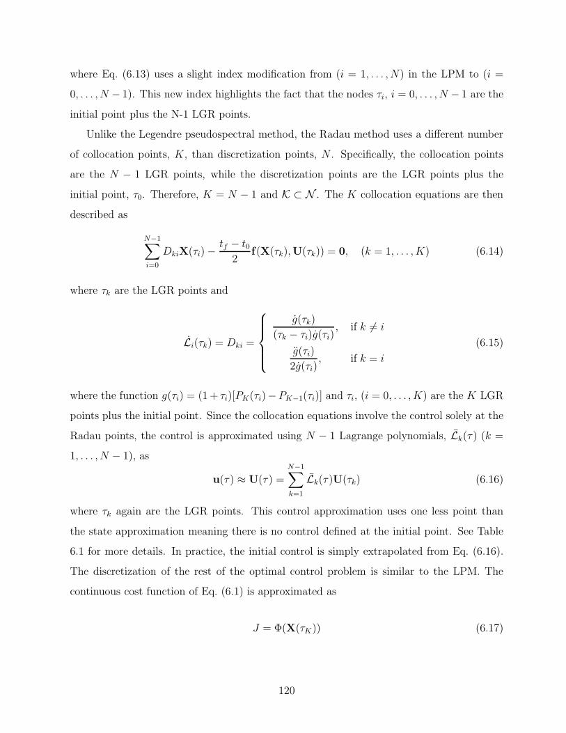
where Eq. (6.13) uses a slight index modification from (i = 1, . . . , N) in the LPM to (i =
0, . . . , N − 1). This new index highlights the fact that the nodes τi, i = 0, . . . , N − 1 are the
initial point plus the N-1 LGR points.
Unlike the Legendre pseudospectral method, the Radau method uses a different number
of collocation points, K, than discretization points, N . Specifically, the collocation points
are the N − 1 LGR points, while the discretization points are the LGR points plus the
initial point, τ0. Therefore, K = N − 1 and K ⊂ N . The K collocation equations are then
described as
N−1∑
i=0
DkiX(τi) −tf − t0
2f(X(τk),U(τk)) = 0, (k = 1, . . . , K) (6.14)
where τk are the LGR points and
Li(τk) = Dki =
g(τk)
(τk − τi)g(τi), if k 6= i
g(τi)
2g(τi), if k = i
(6.15)
where the function g(τi) = (1 + τi)[PK(τi)−PK−1(τi)] and τi, (i = 0, . . . , K) are the K LGR
points plus the initial point. Since the collocation equations involve the control solely at the
Radau points, the control is approximated using N − 1 Lagrange polynomials, Lk(τ) (k =
1, . . . , N − 1), as
u(τ) ≈ U(τ) =N−1∑
k=1
Lk(τ)U(τk) (6.16)
where τk again are the LGR points. This control approximation uses one less point than
the state approximation meaning there is no control defined at the initial point. See Table
6.1 for more details. In practice, the initial control is simply extrapolated from Eq. (6.16).
The discretization of the rest of the optimal control problem is similar to the LPM. The
continuous cost function of Eq. (6.1) is approximated as
J = Φ(X(τK)) (6.17)
120

Recall that in the Radau method, the final LGR point τK = 1. Lastly, the boundary
constraint of Eq. (6.3) is expressed as a function of the initial point and the final point as
φ(X(τ0),X(τK)) = 0 (6.18)
The cost function of Eq. (6.17) and the algebraic constraints of Eqs. (6.14) and (6.18) define
an NLP whose solution is an approximate solution to the continuous Mayer problem.
6.3.3 Gauss Pseudospectral Method (GPM)
This section largely echoes Chapter 3, however slight differences in index notation are in-
duced to highlight nuances between this method and the Legendre and Radau pseudospectral
methods. Recall from Chapter 3 that the location of the nodes in the Gauss pseudospectral
method are based on Legendre-Gauss (LG) points, which lie on the interval τ ∈ (−1, 1).
This set of points includes neither the initial point nor the final point. Therefore, in order to
fully discretize the time interval, the N discretization points are (N − 2) interior LG points,
the initial point, τ0 ≡ −1, and the final point, τF ≡ 1. The state is approximated using a
basis of N-1 Lagrange interpolating polynomials, which is slightly smaller than the previous
two methods,
x(τ) ≈ X(τ) =N−2∑
i=0
Li(τ)X(τi) (6.19)
where τi (i = 0, . . . , N−2) are the initial point plus the (N−2) LG points. Note that the final
point, although it is part of the NLP discretization, is not part of the state approximation.
This results in a state approximation that is one order less than the previous methods, but is
necessary in order to have the equivalence property between the KKT conditions and HBVP
conditions. As in the Radau pseudospectral method, the Gauss pseudospectral method uses
a different number of collocation points, K, than discretization points, N . Specifically, the
collocation points are the LG points, while the discretization points are the LG points plus
the initial point and final point. Therefore, K = N − 2 and K ⊂ N . The K collocation
121

equations are then described as
N−2∑
i=0
DkiX(τi) −tf − t0
2f(X(τk),U(τk)) = 0, (k = 1, . . . , K) (6.20)
where τk, (k = 1, . . . , K) are the LG points. This equation is exactly the same as Eq. (3.7)
in Chapter 3 except for a slight change in indices to show the relationship of this collocation
approach to the others presented in this chapter. Note that there is no collocation at either
boundary. The control is approximated at the (N − 2) collocation points using a basis of
(N − 2) Lagrange interpolating polynomials Li(τ), (i = 1, . . . , N − 2) as
u(τ) ≈ U(τ) =N−2∑
i=1
Li(τ)U(τi) (6.21)
where τi, (k = 1, . . . , N − 2) are the LG points. Table 6.1 lists all the Lagrange polynomial
expressions described in this work.
As explained in Chapter 3, an additional constraint must be added to the discretization
in order to ensure that the the final state obeys the state dynamics. This is enforced by
including a Gauss quadrature to approximate the integral of the dynamics across the entire
interval (Eq. (3.4)):
X(τF ) − X(τ0) −tf − t0
2
K∑
k=1
wkf(X(τk),U(τk)) = 0 (6.22)
where wk are the Gauss weights and τk are the LG points. Lastly, the cost function is
approximated by
J = Φ(X(τF )) (6.23)
and the boundary constraint is expressed as
φ(X(τ0),X(τF )) = 0 (6.24)
The cost function of Eq. (6.23) and the algebraic constraints of Eqs. (6.20), (6.22), and (6.24)
define an NLP whose solution is an approximate solution to the continuous Mayer problem.
122

Table 6.1: Definitions of Lagrange interpolation polynomials used in this work# of Basis Polynomials Application Symbol Index
N LPM (x,u,λ) Li(τ) i = 1, . . . , NN RPM (x) Li(τ) i = 0, . . . , N − 1
N-1 RPM (u, λ) Li(τ) i = 1, . . . , N − 1N-1 GPM (x,λ) Li(τ) i = 0, . . . , N − 2
N-2 GPM (u) Li(τ) i = 1, . . . , N − 2
6.4 Costate Estimation
All three aforementioned pseudospectral methods have established costate estimation proce-
dures. In particular, a mapping between the KKT multipliers of the NLP and the costates
of the continuous-time optimal control problem has been derived for all three methods. This
section describes the costate estimation procedure for each method.
Legendre Pseudospectral Method
As explained in Chapter 3, the KKT conditions of the NLP are derived by defining an aug-
mented cost function, which brings the NLP constraints into the cost function via Lagrange
multipliers. For LPM, the augmented cost is
Ja = Φ(XN) − νT φ(X1,XN) −K∑
k=1
ΛT
k
(
N∑
i=1
DkiXi −tf − t0
2f(Xk,Uk)
)
(6.25)
The KKT multipliers in Eq. (6.25) are Λk, (k = 1, . . . , K), which are associated with
the collocation equations of Eq. (6.9) and ν, which relates to the boundary condition of
Eq. (6.12). Without going into detail, the mapping from the KKT multipliers to the HBVP
variables is:39
Λk =Λk
wk, (k = 1, . . . , K)
ν = ν
(6.26)
123

The HBVP variables Λk, (k = 1, . . . , K), and ν, now defined in terms of NLP multipliers,
can be substituted into the HBVP equations to determine if the optimality conditions have
been met. It has been documented in the literature49,128 that this mapping for the LPM
does not provide an exact equivalence between the KKT conditions and the HBVP condi-
tions. Specifically, the HBVP costate differential equations are not naturally collocated at
the boundaries, meaning the boundary KKT conditions result in a linear combination of
two HBVP conditions: the boundary costate dynamics and the transversality conditions.
Although all the KKT conditions are not derived here, the conflicting KKT condition is
shown, which is found by taking the partial derivative of the augmented cost function with
respect to the initial state:
K∑
k=1
ΛTk D1k +
tf − t02
ΛT1
∂f1∂X1
=1
w1
(
−ΛT1 + νT ∂φ
∂X1
)
(6.27)
Notice that the left-hand side of the equation resembles the discretized costate dynamics and
the right hand side resembles the transversality condition from the HBVP in Section 6.2. If
these conditions were to map exactly to the HBVP equations, each side of Eq. (6.27) should
equal zero. However, Eq. (6.27) is inseparable in the LPM. Similarly, the KKT condition
corresponding to the final state is
K∑
k=1
ΛTk DNk +
tf − t02
ΛTN
∂fN∂XN
=1
wN
(
ΛTN − ∂Φ
∂XN
+ νT ∂φ
∂XN
)
(6.28)
where again, the left-hand side is the discretized costate dynamics and the right-hand side
is the transversality condition corresponding to the terminal state. It is impossible to get
an exact mapping from the KKT conditions to the HBVP conditions without being able
to separate these mixed conditions. Recent research49 suggests that by applying relaxation
techniques, linear independence constraint qualification, and an additional set of conditions
called “closure conditions”, one can show that there exists a costate approximation that
converges to the true costate in the limit. From Ref. 49, the most recent closure conditions
124

are∥
∥
∥
∥
∥
−Λ∗1 −
∂Φ
∂x1
T
(X∗1,X
∗N) −
(
∂φ
∂x1
(X∗1,X
∗N)
)T
ν∗
∥
∥
∥
∥
∥
∞
≤ δD
∥
∥
∥
∥
∥
Λ∗N − ∂Φ
∂xN
T
(X∗1,X
∗N) −
(
∂φ
∂xN
(X∗1,X
∗N)
)T
ν∗
∥
∥
∥
∥
∥
∞
≤ δD
(6.29)
where X∗, Λ∗, and ν∗ represent a solution that satisfies Eq. (6.29) and the KKT conditions.
δD is a dual feasibility tolerance. These conditions are essentially the discretized HBVP
transversality conditions.73 The covector mapping theorem49 states that there exists an N
large enough so that the closure conditions and the KKT conditions are satisfied to a specified
tolerance, δ. Upon close examination of Ref. 49 (and the references therein) any algorithm
attempting to solve the combined KKT conditions and closure conditions must solve a mixed
primal-dual feasibility problem. By including the closure conditions of Eq. (6.29) to form the
“augmented optimality conditions”, both the state and costate are now variables to be solved.
This procedure significantly increases the computational complexity required to estimate the
costate. To be thorough, both LPM costate approximations described here (Refs. 39 and 49)
are considered in this chapter. The LPM costate is computed first according to Eq. (6.26),
and then by formulating the primal-dual feasibility problem which attempts to satisfy the
augmented KKT conditions according to some tolerance, δ. It is noted that improving the
LPM costate approximation is an ongoing research topic, and better methods may be found
in the future.
Similar to the LPM state approximation, the continuous-time costate approximation is
represented by a basis of N Lagrange interpolating polynomials as
λ(τ) ≈ Λ(τ) =N∑
i=1
Λ(τi)Li(τ) (6.30)
Radau Pseudospectral Method
The augmented cost function corresponding to the Radau pseudospectral method is given
as
Ja = Φ(XK) − νT φ(X0,XK) −K∑
k=1
ΛT
k
(
K∑
i=0
DkiXi −tf − t0
2f(Xk,Uk)
)
(6.31)
125

The KKT multipliers resulting from the NLP using the Radau pseudospectral method are
Λk, (k = 1, . . . , K), associated with the collocation equations of Eq. (6.14) and ν, associated
with the boundary conditions of Eq. (6.18). The mapping from the KKT multipliers to the
HBVP variables is described as follows:
Λk =Λk
wk, (k = 1, . . . , K)
ν = ν
(6.32)
The K discrete costates Λk, (k = 1, . . . , K), and the HBVP multiplier ν are now defined in
terms of the KKT multipliers. As in the LPM, it is understood that there is an imperfect
match between the KKT multipliers and the costate.72 The Radau method has a similar
conflict of HBVP equations when the partial derivative of the augmented cost function is
taken with respect to the final state:
K∑
k=1
ΛTk DKk +
tf − t02
ΛTK
∂fK∂XK
=1
wK
(
ΛTK − ∂Φ
∂XK+ νT ∂φ
∂XK
)
(6.33)
However, recent work71,72 has demonstrated rapid convergence rates of the costate approxi-
mation using Eq. (6.32) as the number of nodes increases. The discrete values of the costate
are used to construct a continuous-time approximation to the costate, which is represented
by a basis of N − 1 Lagrange interpolating polynomials, as in the control:72
λ(τ) ≈ Λ(τ) =
K∑
i=1
Λ(τi)Li(τ) (6.34)
where τk, (k = 1, . . . , K) are the LGR points. Note that since there is no collocation at
the initial point, there is no initial costate estimate that is directly output from the NLP.
However, the initial costate can be approximated by extrapolating Eq. (6.34).
126
Gauss Pseudospectral Method
The augmented cost function corresponding to the Gauss discretization of the Mayer problem
is
Ja = Φ(XF ) − νT φ(X0,XF ) −K∑
k=1
ΛT
k
(
K∑
i=0
DkiXi −tf − t0
2f(Xk,Uk)
)
−ΛT
F
(
XF −X0 −tf − t0
2
K∑
k=1
wkf(Xk,Uk)
) (6.35)
The KKT multipliers resulting from the NLP using the Gauss pseudospectral method are
Λk (k = 1, . . . , K), associated with the collocation equations of Eq. (6.20), ΛF , associated
with the quadrature constraint of Eq. (3.4), and ν, associated with the boundary conditions
of Eq. (6.24). The mapping from the KKT multipliers to the HBVP variables is described
in Chapter 3 and repeated here for clarity:
Λk =Λk
wk+ ΛF , (k = 1, . . . , K)
ν = ν ,
Λf = ΛF
(6.36)
The variables Λk, Λf , and ν, now defined in terms of NLP multipliers, can be substituted into
the HBVP equations to ensure the optimality conditions have been met. The discrete costate
is then used to construct a continuous-time costate approximation, which is represented by
a slightly different basis of N − 1 Lagrange interpolating polynomials, defined as
λ(τ) ≈ Λ(τ) =K+1∑
i=1
Λ(τi)Li(τ) (6.37)
where τi, (i = 1, . . . , K + 1) are the LG points plus the final point, τF . Recall that the
state is approximated using (N − 1) Lagrange polynomials based on the LG points and the
initial time, while the costate, λ(τ), is approximated using (N − 1) Lagrange polynomials
consisting of the LG points and the final time. This discrepancy is required to preserve the
mapping, as expained in Chapter 3. As in the Radau method, an approximation for the
127

initial costate, Λ0, cannot be pulled directly from a corresponding multiplier in the NLP
because no such multiplier exists. However, an accurate approximation to the initial costate
can be determined from the following equation:
Λ0 ≡ ΛF −K∑
k=1
Dk0Λk (6.38)
which is shown in Chapter 3,to satisfy the HBVP transversality condition
ΛT0 = νT ∂φ
∂X0
(6.39)
resulting in a perfect match between the HBVP equations and the KKT conditions. Fur-
thermore, one could simply extrapolate Eq. (6.37) to τ0, which would produce an equally
accurate initial costate. All three methods for determining the initial costate are equiva-
lent. The remainder of this chapter focuses on comparing these pseudospectral techniques in
terms of their computational efficiency, approximation accuracy, and solution convergence
rates with respect to the state, control, and especially the costate.
6.5 Comparison of Pseudospectral Methods
The three pseudospectral methods described in this chapter: GPM, RPM, and LPM, are
compared on several examples of increasing complexity.
6.5.1 Single State Example
As a first example, consider the following one-dimensional optimal control problem. Minimize
the cost functional
J = −y(tf) (6.40)
subject to the constraints
y(t) = y(t)u(t) − y(t) − u2(t) (6.41)
128

and the initial condition
y(t0) = 1 (6.42)
where y(t), is the state, u(t) is the control, and tf = 5 is the final time. The exact solution
is
y∗(t) =4
1 + 3et(6.43)
λ∗(t) = ae(2 ln(1+3et)−t) (6.44)
u∗(t) = .5y∗(t) (6.45)
where a =−1
(e−5 + 6 + 9e5)(6.46)
(6.47)
λ∗(t) is the costate associated with the optimal solution. The exact solution is depicted in
Fig. 6-1.
y
λ
-1.5
-1
-0.5
0
0
0.5
2 3 4 5
1
1
State
t
u
Figure 6-1: Exact solution for the single state example
This problem is solved by all three pseudospectral techniques mentioned previously. Each
129

method transcribes the optimal control problem into an NLP that consists of 10 nodes
(N = 10). The resulting NLP is then solved with SNOPT45 using the default feasibility
and optimality tolerances (10−6). In Fig. 6-2, the absolute value of the error between the
NLP state and the exact solution (|Y (τi) − y∗(τi)|, i = 1, . . . , N) is plotted for each node
and all three approaches. Note that the error in initial state is not included since the
SNOPT satisfies state equality bounds (i.e., the initial conditions) to double precision (10−16).
When comparing the state accuracy of the three methods in this example, there is no clear
method that outperforms the other two across the entire interval. In fact, the only noticeable
difference in Fig. 6-2 is that both the GPM and RPM formulations produce an extremely
accurate terminal state. It is hypothesized that the highly accurate terminal state for the
GPM is due to the additional quadrature constraint in the NLP.
-9
-10
10
10
10
10
10
10
10
-8
-7
-6
-5
-4
0 2 3 4 51
GPM y
LPM y
RPM y
|Y(t
i)−
y∗ (
t i)|
t
Figure 6-2: State error for the single state example.
The control error is plotted in Fig. 6-3. As described in Section 6.3, each method approx-
imates the control using a different number of points. The LPM discretizes the control at all
N discretization points, while Radau discretizes the control at the (N-1) Radau points, and
the Gauss method discretizes the control at the (N-2) Gauss points. In the Radau discretiza-
130
tion, the initial control is missing. Similarly, in the Gauss discretization, the control at both
the initial and final time are missing. These missing control values can be computed by a
variety of techniques. The approach often outlined in the literature33,71 is to extrapolate
the control approximation equations, Eqs. (6.10), (6.16) and (6.21). However, in practice
it is more common to use a simple spline extrapolation.14 Thirdly, a technique involving
the HBVP equations67 at the boundaries has been developed for the Gauss pseudospectral
method in Chapter 4, but this technique is not used in this section. Since the extrapolated
controls are not explicit variables in the NLP, one would assume that they would be less
accurate than methods that include the boundary controls in the formulation of the NLP,
such as the LPM. In Fig. 6-3, the boundary control estimate for the Gauss method is in-
deed the least accurate. Likewise, the accuracy of the initial control estimate for the Radau
method is similar to the GPM value. However, it is interesting that while the largest error
for Gauss and Radau are at the boundaries, the LPM has a larger error at one of the interior
points. In this example, the benefit of an accurate initial control for the LPM is offset by
the inaccurate interior control.
A more appropriate way to determine the effect of the control error is to actually propa-
gate the state dynamics according to the control estimate from the NLP, as done in Chapter 4.
In this comparison, the state dynamics are propagated using the Matlab function ODE45,
where the control approximations are represented using Eqs. (6.10), (6.16), and (6.21). The
resulting propagated state error is shown in Fig. 6-4. Clearly, the LPM propagation error is
the largest despite the relatively accurate boundary controls.
The largest discrepancy between the methods is seen in the costate comparison of Fig. 6-
5. The LPM costate approximation is several orders of magnitude worse than the other
two methods across all values of N . This example highlights a common problem49 with the
original LPM costate approximation39 where the approximation tends to “wiggle” about the
true solution, shown clearly in Fig. 6-6. Furthermore, note that the largest error in the LPM
costate occurs at the boundaries due to the conflicting constraints (explained in Section 6.4).
The GPM, which has no constraint conflict, provides extremely accurate boundary costates,
while the RPM produces an accurate initial costate (no conflict) but a less accurate final
costate (which has a conflict explained in Section 6.4).
131
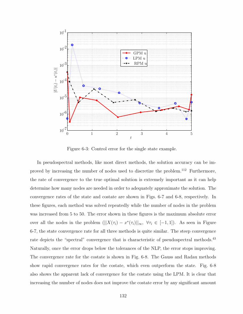
10
10
10
10
10
10
10-7
-6
-5
-4
-3
-2
-1
0 2 3 4 51t
GPM u
LPM u
RPM u
|U(t
i)−
u∗ (
t i)|
Figure 6-3: Control error for the single state example.
In pseudospectral methods, like most direct methods, the solution accuracy can be im-
proved by increasing the number of nodes used to discretize the problem.112 Furthermore,
the rate of convergence to the true optimal solution is extremely important as it can help
determine how many nodes are needed in order to adequately approximate the solution. The
convergence rates of the state and costate are shown in Figs. 6-7 and 6-8, respectively. In
these figures, each method was solved repeatedly while the number of nodes in the problem
was increased from 5 to 50. The error shown in these figures is the maximum absolute error
over all the nodes in the problem (||X(τi) − x∗(τi)||∞, ∀τi ∈ [−1, 1]). As seen in Figure
6-7, the state convergence rate for all three methods is quite similar. The steep convergence
rate depicts the “spectral” convergence that is characteristic of pseudospectral methods.43
Naturally, once the error drops below the tolerances of the NLP, the error stops improving.
The convergence rate for the costate is shown in Fig. 6-8. The Gauss and Radau methods
show rapid convergence rates for the costate, which even outperform the state. Fig. 6-8
also shows the apparent lack of convergence for the costate using the LPM. It is clear that
increasing the number of nodes does not improve the costate error by any significant amount
132

-10
-12
-14
10
10
10
10
10
10
-8
-6
-4
0 2 3 4 51
Magnitude
t
|y pro
p(t
)−
y∗ (
t)|
GPM
RPM
LPM
Figure 6-4: Error in the propagated state for the single state example.
for this example. As mentioned previously, Gong and Ross have devised a modified covector
mapping theorem to improve the costate approximation for the LPM. This covector map-
ping theorem includes a set of “closure conditions” that is assumed to be implemented in a
mixed primal-dual feasibility problem where the variables are the state, control, and costate.
The constraints in this primal-dual feasibility problem are the KKT conditions of the NLP
and the additional closure conditions. When this alternate NLP is posed and solved, the
resulting costate convergence rate in Fig. 6-9 is indeed much better, although not as rapid
as either the Gauss or Radau methods. As mentioned previously, this increased accuracy
comes at a significant computational burden in post-processing. Due to the large number of
extra steps necessary to produce this result, further computation of LPM costates involves
only the original costate estimation procedure of Eq. (6.26), since this is the likely method
to be used in practice.
Lastly, Fig. 6-10 depicts the convergence rate of the error in the final control, u(tf ). For
this figure, the final control in the GPM was computed following the approach described in
Chapter 4, and the final control for the RPM and LPM methods are simply output from the
133
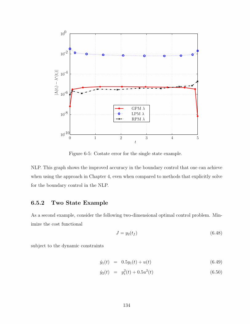
-10
10
10
10
10
10
10
-8
-6
-4
-2
0
0 2 3 4 51t
|Λ(t
i)−
λ∗ (
t i)|
GPM λ
RPM λ
LPM λ
Figure 6-5: Costate error for the single state example.
NLP. This graph shows the improved accuracy in the boundary control that one can achieve
when using the approach in Chapter 4, even when compared to methods that explicitly solve
for the boundary control in the NLP.
6.5.2 Two State Example
As a second example, consider the following two-dimensional optimal control problem. Min-
imize the cost functional
J = y2(tf ) (6.48)
subject to the dynamic constraints
y1(t) = 0.5y1(t) + u(t) (6.49)
y2(t) = y21(t) + 0.5u2(t) (6.50)
134

−0.04
−0.03
−0.02
−0.01
0.01
0.02
0.03
λ err
0
0 2 3 4 51t
Λ(t
i)−
λ∗ (
t i)
Figure 6-6: LPM costate error for the single state example.
and the boundary conditions,
y1(t0) = 1 y1(tf ) = 0.5 (6.51)
y2(t0) = 0 (6.52)
where tf = 5. Note that this problem contains a terminal bound on the first state, y1(tf ).
The exact solution is of the form
y∗1(t) = a1e
1.5t + a2e−1.5t, (6.53)
y∗2(t) = a3(e
1.5t)2 − a4(e−1.5t)2 + c1, (6.54)
λ∗1(t) = a5e
1.5t + a6e−1.5t, (6.55)
λ∗2(t) = 1, (6.56)
u∗(t) = −λ∗1(t) (6.57)
The exact solution can be seen in Fig. 6-11. Again, all three methods are compared using 10
135

-10
10
10
10
10
10
1010 2015 25 30 35 40 45
N
-8
-6
-4
-2
0
5 50
GPM yLPM yRPM y
||Y(t
i)−
y∗ (
t i)| ∞
Figure 6-7: State convergence for the single state example
nodes. The error plots are formulated in the same manner as the previous example problem.
Fig. 6-12 shows the state error at each node for all three methods. Recall that the error for
the states involving the boundary conditions is O(10−16), and therefore outside the range of
the plot. As in the single-state example, all three methods are relatively comparable in state
accuracy. Moreover, the GPM and Radau formulations again show an increase in accuracy
for the unconstrained terminal state.
The control error is plotted in Fig. 6-13. Interestingly, for this problem, the LPM control
estimate is worse than both GPM and RPM, even at the boundaries. The NLP control for
each method is used to propagate the state equations, and their resulting state accuracy is
compared in Fig. 6-14 for both states. In this example, the RPM produces the most accurate
propagated solution, followed by the GPM, and lastly LPM.
Reconfirming the results in the first example, the largest discrepancy between the meth-
ods is seen in the costate comparison, and specifically with the second costate, shown in
Fig. 6-15. The LPM method produces the worst costate approximation for both λ1 and
136

10
10
10
10
10
10
10
1010 2015 25 30 35 40 45
N
-8
-7
-6
-5
-4
-3
-2
-1
5 50
GPM λ
RPM λ
LPM λ
||Y(t
i)−
y∗ (
t i)| ∞
Figure 6-8: Costate convergence for the single state example
λ2. Although it is not shown, this large error in λ2 exhibits the same “wiggle” phenomenon
around the true costate as seen in the first example. In terms of boundary costates, the GPM
method provides the most accurate boundary costates, and the Radau method provides a
relatively accurate initial costate, but an inaccurate final costate, as expected from the the-
oretical analysis. In the Radau method, the final costate is consistently the least accurate
costate, suggesting that the conflicting HBVP equations described in Section 6.4 degrades
the performance of this method.
The convergence rates of the state and costate are shown in Figs. 6-16 and 6-17, respec-
tively. Each approach was solved repeatedly while the number of nodes in the problem was
increased from 5 to 30. The error shown in these figures is computed in the same manner
as the previous example. Fig. 6-16 displays both states, y1 and y2, and there is a noticeable
difference between the convergence rate of y1 and y2 for the GPM and RPM. However, for the
LPM approach, both states converge at the same (slower) rate. The state convergence rate
of the RPM is the fastest for this example. It is hypothesized that this slight improvement
137
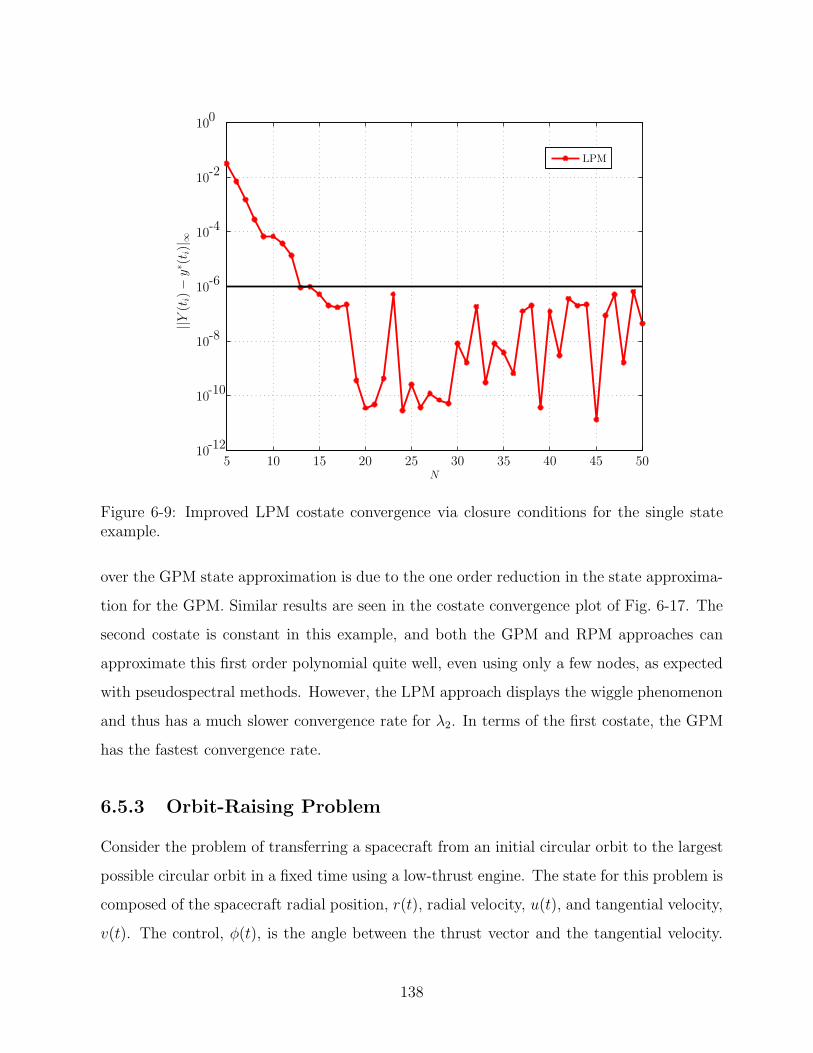
10
10
10
10
10
10
1010 2015 25 30 35 40 45
N
-8
-6
-4
-2
0
5 50
||Y(t
i)−
y∗ (
t i)| ∞
-10
-12
LPM
Figure 6-9: Improved LPM costate convergence via closure conditions for the single stateexample.
over the GPM state approximation is due to the one order reduction in the state approxima-
tion for the GPM. Similar results are seen in the costate convergence plot of Fig. 6-17. The
second costate is constant in this example, and both the GPM and RPM approaches can
approximate this first order polynomial quite well, even using only a few nodes, as expected
with pseudospectral methods. However, the LPM approach displays the wiggle phenomenon
and thus has a much slower convergence rate for λ2. In terms of the first costate, the GPM
has the fastest convergence rate.
6.5.3 Orbit-Raising Problem
Consider the problem of transferring a spacecraft from an initial circular orbit to the largest
possible circular orbit in a fixed time using a low-thrust engine. The state for this problem is
composed of the spacecraft radial position, r(t), radial velocity, u(t), and tangential velocity,
v(t). The control, φ(t), is the angle between the thrust vector and the tangential velocity.
138

10
10
10
10
10
1010 2015 25 30 35 40 45
N
-8
-6
-4
-2
5 50
GPM
RPM
LPM
-10
-12
|U(t
f)−
u∗(t
f)|
Figure 6-10: Convergence of the final control, u(tf), for the single state example.
The optimal control problem is stated as follows. Minimize the cost functional
J = −r(tf ) (6.58)
subject to the dynamic constraints
r = u
u =v2
r− µ
r2+
T sin φ
m0 − |m|t
v = −uv
r+
T cos φ
m0 − |m|t
(6.59)
139

y
y
λ
λ
-2
-1.5
-1
-0.5
0
0
0.5
1.5
2
2
2
2 3 4 5
1
1
1
1t
u
Figure 6-11: Exact solution for the two state example.
and the boundary conditions
r(0) = 1, r(tf ) = free
u(0) = 0, u(tf ) = 0,
v(0) =
√
µ
r(0), v(tf ) =
√
µ
r(tf),
(6.60)
where µ is the gravitational parameter, T is the thrust magnitude, m0 is the initial mass,
and m is the fuel consumption rate. These parameters are given as follows in normalized
units:
T = 0.1405, m = 0.0749, m0 = µ = 1, tf = 3.32 (6.61)
This problem does not have an analytic solution, but it has been solved numerically many
times6,20 so it’s solution is well known. The results of each method was compared against
the solution to a boundary value problem solution using the Matlab function BVP4C with
a tolerance of 10−9. For brevity, an error analysis is presented for only the first state and
costate, r(t) and λr(t). The remaining state and costate errors look very similar to the
140

10
10
10
10
10
10
10-8
-7
-6
-5
-4
-3
-2
0 2 3 4 51
|Y(t
i)−
y∗ (
t i)|
t
GPM y1
LPM y1
RPM y1
GPM y2
LPM y2
RPM y2
Figure 6-12: State error for the two state example
one presented. Fig. 6-18 shows the state error throughout the trajectory. The RPM has a
slightly better state accuracy than the other two methods, although they all have very similar
maximum state errors. Interestingly, in Fig. 6-19, the RPM also has a slightly better costate
approximation than the other two methods and does not exhibit the usual reduced costate
accuracy at the terminal time. As in the previous examples, the LPM costate convergence
rate is significantly worse than the other two methods, shown in Fig. 6-20. Note that the
convergence rates for the Radau and Gauss methods are slower than in the previous examples
due to a discontinuity in the optimal control profile.
6.6 Rationale for Choosing a Method
Based on the results of all three example problems and a detailed analysis of the mathematics
of each method, there may be certain circumstances under which each method should be
chosen. Inaccurate boundary costates in the LPM method are attributed to boundary costs
or constraints in the problem. However, if the original problem has no boundary constraints
141

10
10
10
10
10-5
-4
-3
-2
-1
0 2 3 4 51t
GPM u
LPM u
RPM u
|U(t
i)−
u∗ (
t i)|
Figure 6-13: Control error for the two state example.
or costs, then the conflicting HBVP equations disappear and LPM would be an appropriate
method. The RPM costate inaccuracy only occurs at the terminal time, so problems without
terminal constraints would likely mitigate the errors in the final costate. The GPM has a
perfect mapping with the HBVP equations, and therefore creates accurate costate estimates
for general problems with both initial and final constraints.
Lastly, Table 6.2 presents NLP computation times for all three examples and all three
methods. The results listed correspond to a Pentium 4, 3.2 GHz machine, where the con-
straint Jacobian was computed using numerical derivatives. All three methods have very
similar computation times, which is expected since the methods are very similar in terms
of their problem density. Note that the codes used in this analysis are not optimized for
computational efficiency. Streamlined coding, analytic derivatives (or automatic differentia-
tion), and a transition to faster programming languages like C or Fortran would significantly
improve the computation times of all three methods.
142

-9
10
10
10
10
10
10
10
10
10
-8
-7
-6
-5
-4
-3
-2
0 2 3 4 51t
|y pro
p(t
)−
y∗ (
t)|
-10
GPM y1
LPM y1
RPM y1
GPM y2
LPM y2
RPM y2
Figure 6-14: Error in the propagated state for the two state example
Table 6.2: CPU Times for each example and each method, in seconds
GPM RPM LPM
Ex 1 (N = 50) 4.265 4.203 4.750Ex 2 (N = 30) 2.203 2.296 2.688Ex 3 (N = 40) 3.969 4.046 5.156
6.7 Summary
This chapter compared three established pseudospectral methods that are used to numeri-
cally solve optimal control problems. In particular, the Legendre, Radau, and Gauss pseu-
dospectral methods have been compared in terms of their accuracy in the state, control,
and costate. Three examples are used in the study to identify the key differences between
the three methods. The results of this comparison indicate that the accuracy of the Radau
and Gauss methods are very similar in accuracy, and both of these methods significantly
outperform the Legendre method in terms of costate accuracy. Furthermore, it is found that
the computational efficiency of all three methods is comparable.
143

10
10
10
10
10
10
-8
-6
-4
-2
0
0 2 3 4 51t
|Λ(t
i)−
λ∗ (
t i)|
(ti
-10
GPM λ1
RPM λ1
LPM λ1
GPM λ2
RPM λ2
LPM λ2
Figure 6-15: Costate error for the two state example
10
10
10
10
10
10
10
1010 2015 25 30
N
-7
-6
-5
-4
-3
-2
-1
0
5
||Y(t
i)−
y∗ (
t i)| ∞
GPM y1LPM y1RPM y1GPM y2
LPM y2
RPM y2
Figure 6-16: State convergence for the two state example
144

10
10
10
10
10
1010 2015 25 30
N
-8
-6
-4
-2
0
5
||Y(t
i)−
y∗ (
t i)| ∞
-10
GPM λ1
RPM λ1
LPM λ1
GPM λ2
RPM λ2
LPM λ2
Figure 6-17: Costate convergence for the two state example
-9
10
10
10
10
10
10
-8
-7
-6
-5
-4
0 0.5 1.5 2 2.5 3 3.51t
|R(t
)−
r∗(t
)|
GPM r
LPM r
RPM r
Figure 6-18: Error in state r(t) for the orbit raising problem
145

λr
λr
Radau λr
10
10
10
10
10
10
10
10-6
-5
-4
-3
-2
-1
0
0 0.5 1.5 2 2.5 3 3.5
1
1t
GPM
LPM
|Λr(t
)−
r∗(t
)|
Figure 6-19: Error in the costate λr(t) for the orbit raising problem
Costate Convergence (λr)
10
10
10
10
10
10
10
10
1010 20 30 40
-6
-5
-4
-3
-2
-1
0
2
1
50 60 70 80 90 100t
|Λr(t
)−
r∗(t
)| GPM λr
LPM λr
RPM λr
Figure 6-20: Convergence of costate λr for the orbit raising problem
146

Chapter 7
Tetrahedral Formation Flying
This chapter applies the Gauss pseudospectral method to a novel research area within
aerospace engineering: spacecraft formation flying. Relatively little is known about the
trajectories of satellites flying in formation, and even less is known about fuel optimal tra-
jectories. The problems considered in this chapter are in reference to the Magnetospheric
Multiscale (MMS) misson, which is an Earth-orbiting formation of four spacecraft working
in close proximity of each other in order to study the Earth’s magnetosphere. Two forma-
tion flying problems are posed in this chapter: an orbit insertion problem, simulating the
fuel-optimal transfer from a parking orbit to the desired mission orbit, and a reconfiguration
problem, where the formation has been significantly degraded and must optimally maneuver
in order to meet the formation constraints created by the science users and minimize the total
fuel used. The problems are solved using the Gauss pseudospectral method and the results
are analyzed that provide new insight into the relative motion of tetrahedral formations.
7.1 Overview of Spacecraft Formation Configuration
Problem
Consider the problem of maneuvering a fleet of four spacecraft from an initial parking orbit
to a terminal reference orbit where the formation must attain a desired tetrahedral shape at
a specified point in the terminal reference orbit. For simplicity, assume that each spacecraft
147

Burn
Bur
n
Coast
Coast
Coast
Start
End
Figure 7-1: Schematic of trajectory event sequence for the orbit insertion problem
is initialized at the same point, (i.e., deployed simultaneously) on a circular parking orbit of
altitude h0 = 600 km and inclination i0 = 28 deg. The desired terminal reference orbit is
600 km by 7000 km elliptic orbit with an inclination of 28 deg. Scientific data is taken at
apogee of this reference orbit, meaning that the spacecraft must be in the desired tetrahedral
formation upon reaching apogee. Constraints are placed on both the size and shape of
this tetrahedral formation. Furthermore, it is desired that the spacecraft return to this
tetrahedral formation repeatedly at every apogee.
The trajectory is divided into five phases per spacecraft with the following phase sequence:
coast, burn, coast, burn, and coast. Naturally, the dynamics are different for the coast and
burn phases: there is no thrust during the coast phases, and in the burn phases the thrust is
constant at its maximum value Tmax. At each phase interface the state must be continuous
while the control can be discontinuous. Note that the initial and terminal times of all phases
are free (with the exception, of course, of the first phase where the initial time is fixed to zero).
Fig. 7-1 shows a schematic of the trajectory event sequence. This five-phase trajectory clearly
has two maneuver opportunities. The specifics of the configuration problem are explained
in the following three sections.
148

7.2 Spacecraft Model and Equations of Motion
7.2.1 Spacecraft Model
This problem considers four identical spacecraft each with a dry mass of 200 kg and a fuel
mass of 300 kg. The maneuvers are assumed to be non-impulsive, with the maximum thrust
level of the engine set to 7.015 kN and the engine specific impulse set to 285.7 s. It is noted
that these physical parameters are typical of a standard apogee kick motor.123
7.2.2 Dynamic Model During Thrust Phases
During all thrust phases the state of each spacecraft is modeled using modified equinoctial
elements. The three degree-of-freedom equations of motion for a spacecraft moving over a
spherical nonrotating Earth are given in modified equinoctial elements as5
p =2p
w
√
p
µaθ
P1 =
√
p
µ
−ar cos L + [(w + 1) sinL + P1]aθ
w+ [Q2 sin L − Q1 cos L]
P2an
w
P2 =
√
p
µ
ar sin L + [(w + 1) cosL + P2]aθ
w− [Q2 sin(L) − Q1 cos L]
P1an
w
Q1 =
√
p
µ
(
s2
2w
)
an sin L
Q2 =
√
p
µ
(
s2
2w
)
an cos L
L =√
µp
(
w
p
)2
+
√
p
µ
Q2 sin L − Q1 cos L
wan
(7.1)
where p is the semi-latus rectum, P1, P2, Q1, and Q2 have no geometric definition, and L
is true longitude. Additionally, w = 1 + P1 sin L + P2 cos L, s2 = 1 + Q21 + Q2
2, and ar, aθ,
and an are the perturbing accelerations in the directions of er, eθ, and en where er is the
unit vector in the radial direction, en is the unit vector in the direction normal to the orbital
plane, and eθ = en × er (thereby completing the right-handed system er, eθ, en). For the
application under consideration here, the perturbing accelerations are due entirely to thrust
149
and can be written as
ar =T
mur, aθ =
T
muθ, an =
T
mun, (7.2)
where T is the thrust magnitude, m is the spacecraft mass, and ur, uθ, and un are the er,
eθ, and en components, respectively, of the thrust direction. Finally, the mass flow rate of
the engine is governed by the equation
m = − T
g0Isp(7.3)
where g0 is the sea level acceleration due to gravity and Isp is the specific impulse of the
engine.
7.2.3 Dynamic Model for Coast Phases
By assuming a spherical Earth gravity model, the only equinoctial element that changes with
time during a coast phase is the true longitude, L. In particular, the differential equation
for the true longitude can be written as
L =dL
dt=
õp
p2(1 + P1 sin L + P2 cos L)2 = f(L, p, P1, P2) (7.4)
Observing that all quantities except L in Eq. (7.4) are constant results in a separation of
variables in Eq. (7.4) to give
dt =dL
f(L, p, P1, P2)(7.5)
Integrating both sides of Eq. (7.5) produces
tf − t0 =
∫ Lf
L0
dL
f(L, p, P1, P2)(7.6)
where t0 and tf are the initial and terminal time, respectively, of the coast phase while
L(t0) = L0 and L(tf ) = Lf are the initial and terminal true longitude. Since all other states
150
are constant during a coast phase, the dynamic model for each spacecraft is given as
tf − t0 −∫ Lf
L0
dL
f(L, p, P1, P2)= 0, i = 1, . . . , 4 (7.7)
All other components of the state (i.e., p, P1, P2, Q1, Q2, and m) are treated as constant
optimization parameters. It is noted that, due to additional terminal constraints, the above
model is not used for the final coast phase.
7.2.4 Dynamic Model for Terminal Phase
The terminal constraints in this problem focus largely on the relative position of the space-
craft, and are easily expressed in Cartesian Earth-centered inertial (ECI) coordinates. There-
fore it makes sense to use a dynamic model that is consistent with the mathematical form of
the constraints. Consequently, as opposed to modified equinoctial elements, the dynamics of
each spacecraft in the final coast phase are described using ECI coordinates. This transition
is by no means necessary, but it both reduces the complexity of the analytic derivatives of
the equations of motion and exemplifies the versatility inherent in the Gauss pseudospectral
method. The new dynamic model is given below as
r = v, v = −µr
‖r‖3(7.8)
where r is the position vector measured from the center of the Earth, v is the inertial velocity,
and µ is the gravitational parameter. In order to maintain continuity between the phases,
the Cartesian variables are transformed to modified equinoctial elements at the start of the
final phase and are set equal to the elements at the final time of the previous phase via
linkage conditions,14,57 explained in the next section.
7.3 Constraints
This section describes the many constraints imposed in the orbit insertion problem. Some
constraints are a direct result of the posed problem, while others are specific to the application
151

of the GPM to this problem.
7.3.1 Initial Conditions
All four spacecraft start in the same circular orbit at time t = 0. The initial conditions
corresponding to this orbit are given in orbital elements as
a(0) = Re + h0 , e(0) = 0
i(0) = 28 deg , ω(0) = 270 deg
Ω(0) = 0 , ν(0) = 270 deg
(7.9)
where a is the semi-major axis, e is the eccentricity, i is the inclination, ω is the argument
of perigee, Ω is the longitude of the ascending node, ν is the true anomaly, Re is the radius
of the Earth, and h0 = 600 km is the initial altitude. It is noted that the initial argument
of perigee, ω(0), is chosen to be the same as that of the terminal reference orbit while the
initial true anomaly, ν(0), is arbitrary. The orbital elements in Eq. (7.9) are then converted
to modified equinoctial elements using a transformation To2e (see for example Ref. 5) to
obtain the initial state in modified equinoctial elements as
p(i)(t0) = p0
P(i)1 (t0) = P1,0
P(i)2 (t0) = P2,0
Q(i)1 (t0) = Q1,0
Q(i)2 (t0) = Q2,0
L(i)(t0) = L0
, (i = 1, . . . , 4) (7.10)
where i is the ith spacecraft. Furthermore, the initial mass of each spacecraft is equal to its
maximum value, i.e.,
m(i)(t0) = mmax , (i = 1, . . . , 4) (7.11)
where mmax = 500 kg. Lastly it is noted that for this preliminary analysis, it is reasonable
to assume that all four spacecraft can start at the same initial point without any conflict.
However, if more realism is added to the problem, issues such as collision avoidance must be
152

addressed.
7.3.2 Interior Point Constraints
In order for the state to be continuous at each phase interface, it is necessary to enforce
linkage conditions at the phase boundaries. These linkage conditions are enforced on the
modified equinoctial elements, mass, and time as
p(i)(t(j)f ) = p(i)(t
(j+1)0 )
P(i)1 (t
(j)f ) = P
(i)1 (t
(j+1)0 )
P(i)2 (t
(j)f ) = P
(i)2 (t
(j+1)0 )
Q(i)1 (t
(j)f ) = Q
(i)1 (t
(j+1)0 )
Q(i)2 (t
(j)f ) = Q
(i)2 (t
(j+1)0 )
L(i)(t(j)f ) = L(i)(t
(j+1)0 )
m(i)(t(j)f ) = m(i)(t
(j+1)0 )
t(i)f
(j)= t
(i)0
(j+1)
,(i = 1, . . . , 4)
(j = 1, . . . , P − 1)(7.12)
where j is the jth phase and P is the number of phases in the problem (in this case P =
5). Finally, in order to ensure that time is increasing during the trajectory, the following
inequality constraint is placed on time during each phase:
t(i)f
(j) − t(i)0
(j) ≥ 0, (i = 1, . . . , 4) , (j = 1, . . . , P ) (7.13)
7.3.3 Path Constraints
The following two path constraints are imposed on the four spacecraft. First, during the
thrust phases of the trajectory it is necessary to constrain the thrust direction to be unit
length. Defining the thrust direction as uT = [ur uθ un]T , the following constraint is imposed
on uT :
uT · uT = 1 (7.14)
Second, during flight the mass of each spacecraft cannot fall below the vehicle dry mass.
Defining the dry mass of each vehicle as mdry, the following inequality constraint is imposed
153

on the mass of each spacecraft during the each phase of the trajectory:
m(i)(t) ≥ mdry , (i = 1, . . . , 4) (7.15)
7.3.4 Terminal Constraints
The position of the mesocenter of the formation is defined as
r =1
4
4∑
i=1
r(i) (7.16)
where r(i) is the position of the ith spacecraft as measured from the center of the Earth. At
time tf , the mesocenter must coincide with the apogee of the terminal orbit. Defining the
position of the terminal orbit apogee as ra, this constraint is given as
r(tf ) = ra (7.17)
Similarly, velocity of the mesocenter of the formation is defined as
v =1
4
4∑
i=1
v(i) (7.18)
where v(i) is the velocity of the ith spacecraft. Since six orbital elements are necessary to
completely define an orbit’s characteristics, constraining both the position and velocity of
the mesocenter at t = tf ensures that the mesocenter is on the reference orbit for that instant
in time. Defining the velocity of the reference orbit apogee as va, the constraint imposed on
the velocity of the formation mesocenter is given as
v(tf ) = va (7.19)
Next, the formation must form a tetrahedron upon reaching apogee of the final orbit. To
ensure the quality of this tetrahedron, a set of constraints are formed that take into account
both the formation size and shape. First, it is noted that the spacecraft must be within
154

a certain distance of each other to take useful measurements. Although an average inter-
spacecraft separation of 10 km is considered ideal, acceptable science return is still possible
for average separations ranging from 4 km to 18 km.62,63 For this application, the formation
size is constrained by placing bounds on the formation’s average side length, L.
4 ≤ L ≤ 18 km. (7.20)
In addition to the formation size, the formation shape must meet certain performance criteria.
The metric used to determine the quality of the shape of the formation is called the QR8
Geometric Factor,88 and is given as
QR8 = Va/V∗ (7.21)
where Va is the actual volume of the tetrahedron, and V ∗ is the (ideal) volume of a regular
tetrahedron whose side length is L. It is seen that the QR8 metric contains no sensitivity
to the size of the tetrahedron. For this work, values of QR8 greater than 0.9 are considered
acceptable. Consequently, the following terminal constraint is enforced:
QR8 ≥ 0.9 (7.22)
See Ref. 88 for details on how to compute the QR8 Geometric Factor. Next, in the absence
of perturbations, a spacecraft’s orbit period is solely a function of semi-major axis. In this
case, spacecraft with equal semi-major axes (and therefore equal periods) will return to
their relative positions exactly one period later. Consequently, the entire formation will be
periodic if all spacecraft involved have the same semi-major axis.
a(1)(t(P )f ) = a(2)(t
(P )f ) = a(3)(t
(P )f ) = a(4)(t
(P )f ) (7.23)
Finally, it is required that the trajectories of all four spacecraft terminate at the same time,
i.e.,
t(1)f
(P )= t
(2)f
(P )= t
(3)f
(P )= t
(4)f
(P )(7.24)
155
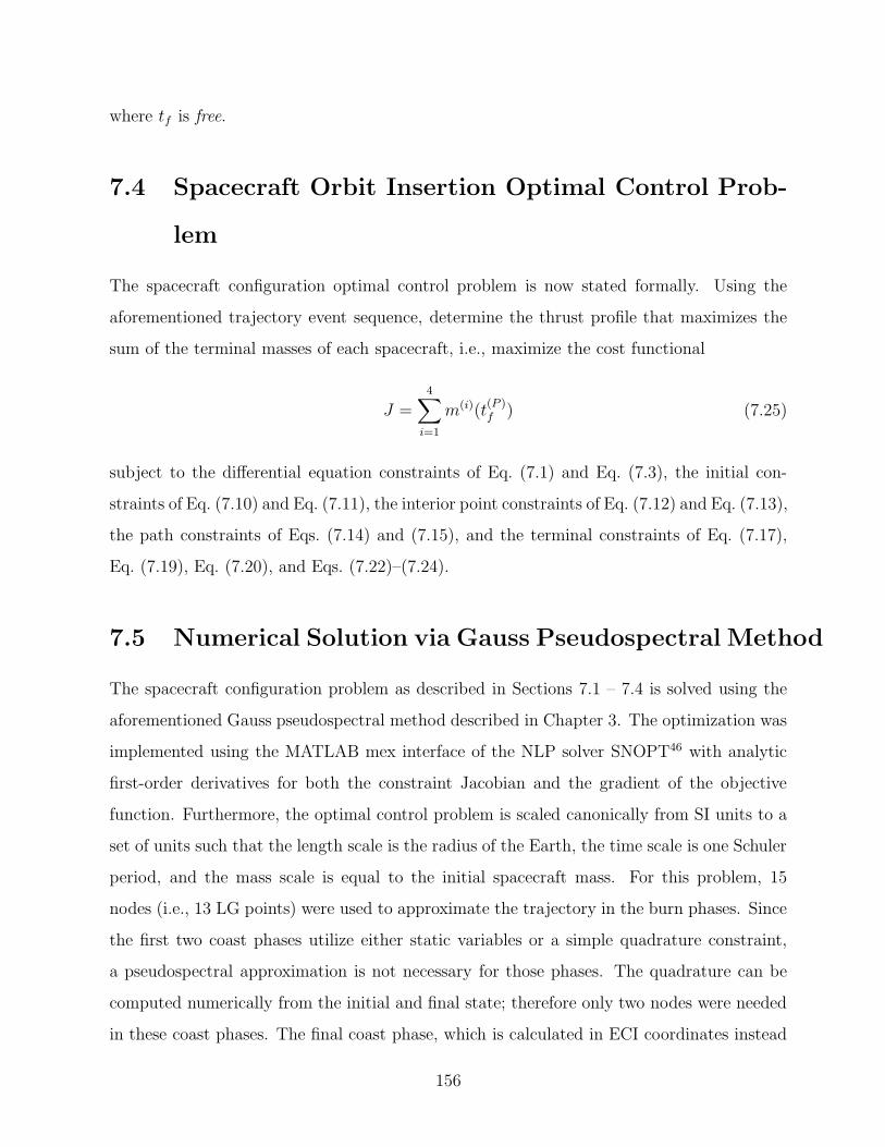
where tf is free.
7.4 Spacecraft Orbit Insertion Optimal Control Prob-
lem
The spacecraft configuration optimal control problem is now stated formally. Using the
aforementioned trajectory event sequence, determine the thrust profile that maximizes the
sum of the terminal masses of each spacecraft, i.e., maximize the cost functional
J =4∑
i=1
m(i)(t(P )f ) (7.25)
subject to the differential equation constraints of Eq. (7.1) and Eq. (7.3), the initial con-
straints of Eq. (7.10) and Eq. (7.11), the interior point constraints of Eq. (7.12) and Eq. (7.13),
the path constraints of Eqs. (7.14) and (7.15), and the terminal constraints of Eq. (7.17),
Eq. (7.19), Eq. (7.20), and Eqs. (7.22)–(7.24).
7.5 Numerical Solution via Gauss Pseudospectral Method
The spacecraft configuration problem as described in Sections 7.1 – 7.4 is solved using the
aforementioned Gauss pseudospectral method described in Chapter 3. The optimization was
implemented using the MATLAB mex interface of the NLP solver SNOPT46 with analytic
first-order derivatives for both the constraint Jacobian and the gradient of the objective
function. Furthermore, the optimal control problem is scaled canonically from SI units to a
set of units such that the length scale is the radius of the Earth, the time scale is one Schuler
period, and the mass scale is equal to the initial spacecraft mass. For this problem, 15
nodes (i.e., 13 LG points) were used to approximate the trajectory in the burn phases. Since
the first two coast phases utilize either static variables or a simple quadrature constraint,
a pseudospectral approximation is not necessary for those phases. The quadrature can be
computed numerically from the initial and final state; therefore only two nodes were needed
in these coast phases. The final coast phase, which is calculated in ECI coordinates instead
156

of equinoctial elements, requires a pseudospectral approximation. Because the duration of
the final coast phase is unknown a priori, 40 nodes (i.e., 38 LG points) were used in the final
coast phase. Note that these node amounts were chosen in order to accurately approximate
the solution yet still maintain a reasonably sized NLP. In the future it is likely that the
number of nodes per phase could become an optimization variable itself. In fact, some more
mature optimization software codes such as SOCS14 do have this feature, but this ability
has not been developed for the GPM.
7.6 Results
The key results of the configuration problem are discussed in this section. The first sub-
section summarizes the results for the two-maneuver configuration problem, and the second
subsection summarizes the results for a single-maneuver configuration problem, where each
spacecraft is given only one maneuver opportunity. Lastly, the third subsection provides a
detailed post-optimality analysis of the single-maneuver solution.
7.6.1 Two-Maneuver Solution
Recall that the formation must attain a geometry that is within 10% of a regular tetrahedron
(measured by the quality factor) and have an average inter-spacecraft distance between 4 and
18km at the terminal time. Furthermore, the spacecraft mesocenter must have a position and
velocity that corresponds to the apogee of the reference orbit, and the spacecraft must have
equal semi-major axes and terminal times. The solution from the NLP does indeed satisfy all
these constraints, and interestingly, the minimum-fuel formation resides at the lower bound
for both the volume constraint and average inter-spacecraft distance. This result is largely
intuitive, since maneuvering the spacecraft to a larger separation distance would naturally
require more fuel, and is counter-productive to the given cost function. Fig. 7-2 provides a
three-dimensional perspective of the terminal tetrahedron where x, y, and z represent the
standard Earth-centered inertial coordinate system.24
Notice in Table 7.1 that, despite the presence of two maneuver opportunities, only one
spacecraft actually thrusts twice. Three of the four spacecraft are able to complete the
157

1.181
1.1812
1.18146.279
6.28
6.281
6.282
6.283
x (m) x 1000y (m)
z (m
)
SC 1
SC 4
SC 2
mesocenter
SC 3
-4 -3 -2 -1 021
Control
Figure 7-2: Three-dimensional view of optimal terminal tetrahedron for two-maneuver prob-lem
Table 7.1: Maneuver durations for the two-maneuver problem
Burn Duration (s) \ Spacecraft Number 1 2 3 4
First Burn 65.1965 65.2958 65.2960 65.1584Second Burn 0 0 0 0.0356
transfer and maintain equal semi-major axes with only the first maneuver. The fourth
spacecraft, however, uses a slight corrective maneuver later in the orbit, at a true anomaly
of approximately 90 deg. Interestingly, as seen in Fig. 7-3, the fourth spacecraft is also the
spacecraft with the lowest final altitude. The small second maneuver is predominantly in
the tangential direction (see Fig. 7-4) and raises the semi-major axis of that spacecraft to
match the other three. With such a small second maneuver, one wonders if two maneuvers
is even necessary. The next section shows that this problem can be solved with only one
maneuver allowed per spacecraft, but the one-maneuver solution uses more fuel than the
two-maneuver trajectory. Further discussion comparing the two scenarios is presented in the
next subsection.
As seen in Fig. 7-5, the optimal locations of the first maneuver for each of the spacecraft
158

500 1500 2000 2500
500
1500
2000
2500SC 2
SC 4
SC 1
SC 3
IncreasingAltitude
Earth
ReferenceOrbit Plane mesocenter
1000
1000
0
0
-500
-500
-1000
-1000
-1500
-1500
-2000
-2000-2500
-2500
y − ymc (m)
z−
z mc
(m)
Figure 7-3: Optimal terminal tetrahedron viewed along the orbital plane for the two-maneuver problem
0
Discrete
0.2
0.4
0.6
0.8
t (s)
Con
trol
Com
pon
ents ur
ut
un
-0.22960.9 2960.91 2960.92 2960.93 2960.94
Figure 7-4: SC #4 control for the 2nd maneuver in the two-maneuver problem
159
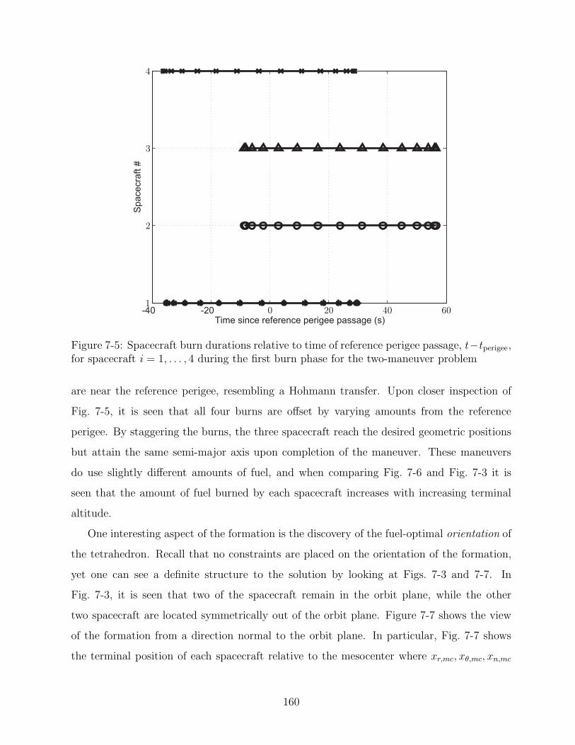
-40 -20Time since reference perigee passage (s)
Spacecra
ft #
20 400
2
3
4
160
Figure 7-5: Spacecraft burn durations relative to time of reference perigee passage, t−tperigee,for spacecraft i = 1, . . . , 4 during the first burn phase for the two-maneuver problem
are near the reference perigee, resembling a Hohmann transfer. Upon closer inspection of
Fig. 7-5, it is seen that all four burns are offset by varying amounts from the reference
perigee. By staggering the burns, the three spacecraft reach the desired geometric positions
but attain the same semi-major axis upon completion of the maneuver. These maneuvers
do use slightly different amounts of fuel, and when comparing Fig. 7-6 and Fig. 7-3 it is
seen that the amount of fuel burned by each spacecraft increases with increasing terminal
altitude.
One interesting aspect of the formation is the discovery of the fuel-optimal orientation of
the tetrahedron. Recall that no constraints are placed on the orientation of the formation,
yet one can see a definite structure to the solution by looking at Figs. 7-3 and 7-7. In
Fig. 7-3, it is seen that two of the spacecraft remain in the orbit plane, while the other
two spacecraft are located symmetrically out of the orbit plane. Figure 7-7 shows the view
of the formation from a direction normal to the orbit plane. In particular, Fig. 7-7 shows
the terminal position of each spacecraft relative to the mesocenter where xr,mc, xθ,mc, xn,mc
160

163.05
163.1
163.15
163.2
163.25
163.3
163.35
163.4
Spacecraft #
Mas
s of
Exp
ende
d F
uel (
kg)
2 3 41
Burn #2
Figure 7-6: Optimal fuel consumption m(i)0 − m
(i)f of spacecraft i = 1, . . . , 4 for the two-
maneuver problem
represent the instantaneous radial, transverse, and normal components of the position of the
mesocenter. It is seen from Fig. 7-7 the two out-of-plane spacecraft (2 and 3) have the same
projection into the orbit plane. Furthermore, the altitude of spacecraft 4, which burns twice,
is significantly lower than the altitude of the other three spacecraft. Although the solution is
not guaranteed to be globally optimal due to the nonconvexity of the problem, it was found
that several different initial guesses all converged to the solution obtained in this analysis.
Figs. 7-8, 7-9, and 7-10 show the maneuver profile for the three components of thrust
for all four spacecraft during the first maneuver. The four arcs in each figure represent the
four spacecraft. Note that Figs. 7-8–7-10 include the control at the boundaries, which was
calculated using the method described in Chapter 4. The overwhelming majority of the
thrust is in the transverse direction (Fig. 7-9), due to the orbit transfer. Consistent with
the relative geometry in Fig. 7-3, only two spacecraft have nonzero normal components of
thrust (Fig. 7-10), since two spacecraft remain in the reference orbit plane. Interestingly,
the small radial component of thrust in all four spacecraft (Fig. 7-8) is negative at the start
161

-4000 2000
SC 1
SC 4
SC 2&3
mesocenter
Earth
0
0-3000
500
1000
1000
-500
-1000
-1000
-1500
-2000-2000
xθ − xθ,mc (m)
xr−
xr,
mc
(m)
Figure 7-7: Optimal terminal tetrahedron viewed from normal to the orbital plane for thetwo-maneuver problem
of the maneuver and positive at the end of the maneuver. By examining Gauss’s variational
equations,5 it is seen that a change in semi-major axis, a, is related to the radial acceleration,
ar by
a =2a2
h
(
e sin(ν)ar +p
raθ
)
(7.26)
where ν is the true anomaly, h is the angular momentum, p is the semilatus rectum, e is the
eccentricity, and r is the radial distance to the spacecraft. From Eq. (7.26) it is seen that
when ν is slightly negative (i.e., just before perigee), the radial acceleration must be negative
in order to increase the semi-major axis. Similarly, when ν is slightly positive (i.e., just after
perigee), the radial acceleration must be positive to increase the semi-major axis. Therefore
starting the maneuver in the negative radial direction before perigee aids in raising the
semi-major axis of the spacecraft. Note that the crossover point for each spacecraft is not
exactly at perigee, but this slight difference is most likely attributed to the need to satisfy
the terminal conditions.
162

-40 -20
0.06
0.08
time since perigee passage
SC 1
SC 2
SC 3
SC 4
SC 2&3
20 40 60
-0.02
-0.04
-0.06
0
0
0.02
0.04
0.1
0.12
ur
Figure 7-8: Radial control for the two-maneuver problem
−40 −20
0.997
0.998
0.999
time since perigee passage
SC 1SC 2SC 3SC 4
SC 2&3
20 40
1
600
0.996
0.995
0.994
0.993
0.992
uθ
Figure 7-9: Transverse control for the two-maneuver problem
163

−40 −20time since perigee passage
SC 1SC 2SC 3SC 4
20 40 60
-0.02
-0.04
-0.01
0
0
0.01
0.02
0.03
0.04
0.05
-0.03
-0.05
un
Figure 7-10: Normal control for the two-maneuver problem
7.6.2 Single-Maneuver Solution
In the two-maneuver solution, only one of the four spacecraft used both maneuver opportu-
nities. Moreover, the spacecraft that did use two maneuvers had an extremely small second
maneuver. A natural question that arises from the two-maneuver result is if the problem can
be solved using only one maneuver opportunity per spacecraft. The one maneuver problem
was posed by setting the duration of the second burn phase to zero.
As expected, slightly more fuel is used in the single-maneuver solution: 653.375 kg as op-
posed to 653.220 kg in the two-maneuver solution. Interestingly, allowing only one maneuver
per spacecraft changes the orientation of the tetrahedron at the terminal time. The orien-
tation of the tetrahedron for the one maneuver solution is seen in Figs. 7-11 and 7-12. By
allowing only one maneuver per spacecraft, the single burn must simultaneously achieve two
conflicting goals. On one hand, at least one spacecraft must terminate at a different altitude
than the other three in order to satisfy the tetrahedral constraints. With the periodicity
constraint, the only way to achieve a different altitude at the final time is by staggering the
164

-2000
0
0
S/C 3
S/C 4
Mesocenter
-1500
2000
2000
1500
1500
1000
1000
500
500
-500
-500
-1000
-1000
S/C 1 & 2
y − ymc (m)
z−
z mc
(m)
Figure 7-11: Optimal terminal tetrahedron viewed along orbital plane for the single-maneuver problem
maneuvers to occur at different times. On the other hand, each spacecraft should burn at
perigee in order to efficiently complete the orbit transfer. To minimize fuel, each spacecraft
should burn as close as possible to perigee, yet still be staggered enough to produce suffi-
cient separation in the final geometry. By balancing these two goals, the resulting effect is
to minimize the maximum altitude separation. This result can be seen in Fig. 7-12, where
the difference between all four spacecraft and the altitude of the mesocenter is the same.
Furthermore, from Fig. 7-13, it can be seen that the maneuvers must be staggered further
away from perigee than in the two-maneuver solution, which is the likely cause of the larger
fuel expenditure than the two-burn solution. Two of the spacecraft burn almost completely
before perigee while the other two are approximately centered around perigee. From a fuel
balancing perspective, the difference in expended fuel between the four spacecraft is 0.25 kg.
In fact, the difference in expended fuel between the four spacecraft for the two-burn solution
is also 0.25 kg, (seen in Fig. 7-6), implying that there is no significant advantage in choosing
one scenario over the other with respect to fuel balancing.
165

-3000xθ − xθ,mc (m)
xr−
xr,
mc
(m)
-2000
0
0
S/C 1S/C 2
Mesocenter
2000
500
1000
1000
1500
-500
-1000
-1000-1500
S/C 3 & 4
3000
Figure 7-12: Optimal terminal tetrahedron viewed from normal to the orbital plane for thesingle-maneuver problem
20-80 -60 0
S/C 1S/C 2S/C 3S/C 4
i
t − tperigee (s)
1
2
3
4
-40 -20 40
Figure 7-13: Spacecraft burn durations relative to time of reference perigee passage, t−tperigee,for spacecraft i = 1, . . . , 4 during the burn phase for the single-maneuver problem
166

7.6.3 Analysis of Optimality for the 1-Maneuver Problem
As mentioned in Section 6.4, a primary benefit of the Gauss Pseudospectral Method is the
equivalence that exists between the direct and indirect approaches.8 By using the costate
mapping shown in this thesis, one can verify that the control from the NLP matches the
analytic control determined from the first-order HBVP optimality conditions at the LG
points (Section 6.2). Confidence in the NLP solution is increased if the NLP solution also
satisfies the HBVP necessary conditions for optimality.
This analysis was done for both the single-maneuver and two-maneuver cases, but only the
results from the single-maneuver case are shown here. Figs. 7-14–7-16 show the magnitude
of the differences between the NLP control and the estimated optimal control derived from
the HBVP conditions for the three components of control, |∆ur|, |∆uθ|, and |∆un|. It is
seen from Figs. 7-14–7-16 that the largest magnitude difference is order 10−6, verifying that
the NLP control is in excellent agreement with the estimated control from the first-order
optimality conditions. This error can potentially be reduced further by increasing the number
of LG points or by tightening the tolerances of the NLP optimizer. Recall that there are
no control variables in the NLP at the boundaries, and therefore only the control at the LG
points are compared.
7.7 Overview of the Spacecraft Reconfiguration Prob-
lem
Now consider a fleet of four spacecraft in a 1.2x12 Earth radii (Re) reference orbit with
a 10 degree inclination. In this scenario, science measurements are taken in a region of
the orbit, called the region of interest (ROI), rather than at a single point as in the orbit
insertion problem. Furthermore, assume that the initial state of each spacecraft is such that
the formation tetrahedron is highly degraded and is incapable of being used to take science
measurements anywhere in this region of interest.62,63 The problem is then to reconfigure the
four spacecraft into a formation such that the formation satisfies a set of geometric constraints
for a portion of the orbit near apogee. This ROI is defined as a portion of the orbit such that
167

200
0
S/C 1
S/C 2
S/C 3
S/C 4
1
2
3
-40 -20 40t − tperigee (s)
-60-80
0.5
1.5
2.5
3.5
|∆u
r|×
10−
6
Figure 7-14: Error in radial control for the single-maneuver problem
the mesocenter (i.e., the geometric center of the formation) is located a distance greater than
9Re from the center of the Earth (roughly ±20 deg in true anomaly on either side of apogee).1
It is known that the initial (degraded) formation does not satisfy the geometric constraints
in the region of interest. The problem considered in this section is to design a single-orbit,
minimum-fuel trajectory and control profile that reconfigures the spacecraft to satisfy both
the required geometric constraints in the region of interest. Furthermore, in order to reduce
interference with the scientific measurements, it is desired that the spacecraft perform no
maneuvers for at least three weeks after the final reconfiguration maneuver. Consequently,
the tetrahedron must be able to maintain the specified quality in the region of interest for at
least three weeks without additional maneuvers. To assess the quality of the tetrahedron well
beyond the final reconfiguration maneuver, the spacecraft are propagated from the terminal
state, x(tf), of the single orbit minimum-fuel trajectory for a period of three weeks under
the influence of several perturbations. The resulting ephemeris of each spacecraft is then
1The region of interest represents the plasma sheet region of the magnetosphere, in which scientificmeasurements are taken.
168

20
0.2
0.4
0.6
0.8
1.2
1.4
1.6
00
S/C 1
S/C 2
S/C 3
S/C 4
1
2
-40 -20 40t − tperigee (s)
-60-80
1.8
|∆u
θ|×
10−
7
Figure 7-15: Error in transverse control for the single-maneuver problem
used to analyze the tetrahedron during this three-week period to see if the region of interest
geometric constraints have been violated. This section addresses and compares minimum-
fuel trajectories that both violate and adhere to this constraint.
Trajectory Event Sequence
The trajectory event sequence for this problem is given as follows. First, the trajectory is
divided into seven phases with the following ordered event sequence:
[Burn Coast Burn Coast Burn Coast ROI]
During the coast phases the thrust is zero, while during the burn phase the thrust is constant
at a maximum value Tmax. Furthermore, at each phase interface it is assumed that the
trajectories and mass of each spacecraft are continuous, but that the control is discontinuous.
It is important to note that, with the exception of the initial time of each spacecraft in the
first phase, the initial and terminal times of each spacecraft and each phase are free. Also,
169

200
0
S/C 1
S/C 2
S/C 3
S/C 4
1
2
3
-40 -20 40t − tperigee (s)
-60-80
0.5
1.5
2.5
3.5
|∆u
n|×
10−
6
Figure 7-16: Error in normal control for the single-maneuver problem
while no maneuvers are allowed in the region of interest phase (and thus the region of interest
phase is a coast phase), several constraints on the formation are applied only in the region of
interest. Therefore, the region of interest is specified separately from the other coast phases
in the problem. Fig. 7-17 shows a schematic of the reconfiguration problem.
7.8 Spacecraft Model and Equations of Motion
7.8.1 Spacecraft Model
In this application four identical spacecraft are considered, each with a dry mass of 150 kg
and a fuel mass of 200 kg. Furthermore, the maximum thrust level of the engine is 0.22 N
with an engine specific impulse of 110 s. These physical parameters are typical of a stan-
dard monopropellant hydrazine orbit maintenance thruster.123 Consequently, all thrusting
maneuvers are assumed to be non-impulsive. Lastly, there are a few parameters that are
not used in the single-orbit optimal control problem, but are used when propagating the
170

Burn
Burn
Bur
n
Coast
Coast
Coast
Start/End
Region of Interest
Reference Orbit
Figure 7-17: Schematic of the event sequence for the reconfiguration problem
spacecraft beyond tf to analyze the long term effects of the tetrahedral formation under
certain perturbations. The drag coefficient, Cd, is 2.2 and the drag area, Ad, is 1 m2 for all
spacecraft.
7.8.2 Equations of Motion
The equations of motion for the reconfiguration problem are exactly the same as those defined
for the orbit insertion problem. Consequently, the dynamic model during thrust phases is
defined in Section 7.2.2, the dynamic model during coast phases is defined in Section 7.2.3,
and the dynamic model for the region of interest is defined in Section 7.2.4.
7.9 Constraints
This section describes the many constraints imposed in the reconfiguration problem. Some
constraints are a direct result of the posed problem, while others are specific to the application
of the GPM to this problem.
171
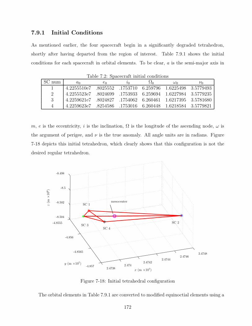
7.9.1 Initial Conditions
As mentioned earlier, the four spacecraft begin in a significantly degraded tetrahedron,
shortly after having departed from the region of interest. Table 7.9.1 shows the initial
conditions for each spacecraft in orbital elements. To be clear, a is the semi-major axis in
Table 7.2: Spacecraft initial conditionsSC num a0 e0 i0 Ω0 ω0 ν0
1 4.2255510e7 .8025552 .1753710 6.259796 1.6225498 3.57794932 4.2255523e7 .8024699 .1753933 6.259694 1.6227984 3.57792353 4.2259621e7 .8024827 .1754062 6.260461 1.6217395 3.57816804 4.2259623e7 .8254586 .1753016 6.260448 1.6218584 3.5779821
m, e is the eccentricity, i is the inclination, Ω is the longitude of the ascending node, ω is
the argument of perigee, and ν is the true anomaly. All angle units are in radians. Figure
7-18 depicts this initial tetrahedron, which clearly shows that this configuration is not the
desired regular tetrahedron.
x (m ×107)
y (m ×107)
z(m
×106
)
2.47382.474
2.47422.4744
2.47462.4748
-4.8555
-4.856
-4.8565
-4.857
-8.504
-8.502
-8.5
-8.498
SC 1
SC 2SC 3
SC 4
mesocenter
Figure 7-18: Initial tetrahedral configuration
The orbital elements in Table 7.9.1 are converted to modified equinoctial elements using a
172
transformation To2e (see for example Ref. 5) to obtain the initial state in modified equinoctial
elements. Furthermore, the initial mass of each spacecraft is set to its maximum value, i.e.,
m(i)(t0) = mmax, i = 1, . . . , 4 (7.27)
where for this problem, mmax = 350 kg.
7.9.2 Interior Point Constraints
The interior point constraints are exactly the same as those defined for the orbit insertion
problem in Section 7.3.2, where the number of phases, P = 7.
7.9.3 Trajectory Path Constraints during Thrust Phases
The path constraints are exactly the same as those defined for the orbit insertion problem
in Section 7.3.3.
7.9.4 Constraints in the Region of Interest Phase
The final phase of the trajectory spans the region of interest. In the region of interest,
several geometric constraints are placed on the formation. As noted in Section 7.7, this
phase is a coast phase. Consequently, the thrust is zero in the region of interest. Next, let
the spacecraft mesocenter (i.e., the mean position) be defined as
r =1
4
4∑
i=1
r(i) (7.28)
where r(i), i = 1, . . . , 4 are the positions of the four spacecraft as measured from the center
of the Earth. At the start of the region of interest phase, the mesocenter must attain a
particular position on the reference orbit, rROI , where ‖rROI‖ = 9Re and is located at a
point prior to apogee. Consequently, a constraint on the position of the mesocenter at the
173

start of the region of interest is given as
r(t(P )0 ) = rROI (7.29)
There is a second constraint enforced at the entrance of the region of interest. In the
absence of perturbations, a spacecraft’s orbit period is solely a function of semi-major axis.
Consequently, a formation in which all spacecraft have equal semi-major axes will be periodic
in its motion. When perturbations are introduced, there will be some degradation to the
tetrahedron over time, but in general the degradation rate is reduced if the orbit periods
are equal at the start. Therefore, in order for the formation to maintain its quality in the
ROI for a period of time into the future (i.e., beyond tf), it is beneficial to require that
the semi-major axes of each spacecraft at the start of the region of interest. Applying this
condition, a second constraint on the formation in the region of interest is given as
a(1)(t(P )0 ) = a(2)(t
(P )0 ) = a(3)(t
(P )0 ) = a(4)(t
(P )0 ) (7.30)
Now, the region of interest terminates when the position of the mesocenter has again attained
a magnitude of 9Re. Consequently, a constraint at the terminus of the region of interest is
given as
||r(t(P )f )|| = 9Re (7.31)
Next, several path constraints are enforced during the region of interest. First, as the
formation evolves in the region of interest, it must maintain a certain geometry in order to be
able to take useful scientific measurements. In particular, the two aspects to the formation
geometry that are important in order to fulfill the science requirements are the shape and
size of the formation. The metric used to determine the quality of the shape of the formation
is the Glassmeier metric (Qgm).88 The Glassmeier metric is given as
Qgm =Va
V ∗+
SAa
SA∗+ 1 (7.32)
where Va is the actual volume of the tetrahedron, SAa is the actual surface area of the
174

tetrahedron, and V ∗ and SA∗ are the volume and surface area, respectively, of a regular
tetrahedron whose average side length is L. It is noted that the largest possible value of
each ratio in Eq. (7.32) is unity. Consequently, the maximum value of Qgm is 3. It is seen
that the Glassmeier quality metric is a function of both volume and surface area of the
tetrahedron. However, because of the functional form of Qgm, the Glassmeier metric has no
sensitivity to the size of the tetrahedron. The ideal geometry for this mission is a regular
tetrahedron with 10 km spacing between each satellite, but science investigators note that
there is considerable flexibility here.62,63 In particular, values of Qgm greater than 2.7 are
acceptable in the region of interest. Consequently, the following path constraint on Qgm is
enforced in the region of interest
Qgm ≥ 2.7 (7.33)
See Appendix for the computation of the Glassmeier quality factor.
Because the Glassmeier metric is insensitive to the size of the tetrahedron, an additional
constraint is required to constrain the size of the tetrahedron. Although an average inter-
spacecraft separation of 10 km is considered ideal, acceptable science return is still possible
for average separations ranging from 4 km to 18 km.62,63 Consequently, the following path
constraint is enforced during the region of interest that keeps the average side length, L,
bounded between its acceptable lower and upper limits:
4 ≤ L ≤ 18. (7.34)
Next, in order to evaluate the aforementioned path constraints in the region of interest at
the same time for all four spacecraft, it is necessary that both the initial and terminal time
for all four spacecraft be the same. Constraints on the initial and terminal time in the region
of interest are then given as
t(1)0
(P )= t
(2)0
(P )= t
(3)0
(P )= t
(4)0
(P )
t(1)f
(P )= t
(2)f
(P )= t
(3)f
(P )= t
(4)f
(P ) (7.35)
It is noted that t0 and tf in these equations are free.
175

7.10 Tetrahedral Reconfiguration Optimal Control Prob-
lem
The optimal control tetrahedral reconfiguration problem is now stated formally. Using the
aforementioned trajectory event sequence, determine the thrust profile that maximizes the
sum of the terminal masses of each spacecraft, i.e., maximize the objective functional
J =4∑
i=1
m(i)(t(P )f ) (7.36)
subject to the dynamic constraints of Eq. (7.1), (7.3), and (7.7), the initial constraints of
Table 7.9.1 and Eq. (7.27), the interior point constraints of Eq. (7.12) and (7.13), the path
constraints of Eq. (7.14) and (7.15), the terminal constraints of Eq. (7.29), (7.30), (7.31),
(7.35), (7.32), and (7.34).
7.11 Numerical Solution via Gauss Pseudospectral Method
The spacecraft configuration problem as described in Section 7.7 - Section 7.10 is solved using
the aforementioned Gauss pseudospectral method.6 The optimization was carried out with
the MATLAB mex interface of the NLP solver SNOPT46 using analytic first-order derivatives
for both the constraint Jacobian and the gradient of the objective function. Furthermore,
the optimal control problem was scaled canonically from SI units to a non-dimensional set of
units such that the length scale is the radius of the Earth, the time scale is one Schuler period,
and the mass scale is equal to the initial spacecraft mass. For this numerical reconfiguration
problem, 10 nodes (i.e., 8 Gauss points) were used for the burn phases, and 50 nodes (i.e., 48
Gauss points) were used in the region of interest coast phase. The coast phases (other
than the region of interest phase) were not discretized, but were computed via numerical
quadrature of Eq. (7.7). Consequently, each coast phase had two nodes representing the
initial and final points of the phase.
Ideally, science investigators would like the formation geometry constraints to hold for a
period of three weeks. Yet, the problem described in the previous sections has a duration of
176

only one orbit, or roughly one day. Because of this, any constraints on the formation after
this first pass through the ROI are not explicitly coded into the problem. However, the solu-
tion to the single-orbit problem was propagated for three weeks using an orbit propagation
tool called FreeFlyer R© to determine the effects of perturbations on the formation. These
results are presented in the following section. The problem was then solved with a tighter
requirement on the tetrahedral formation, which, when propagated for three weeks, met the
tetrahedral requirements for the entire duration. The results of this case are presented in
the following section as well.
7.12 Results
7.12.1 Minimum-Fuel Solution for Qmin = 2.7
A minimum-fuel solution to the problem posed in Section 7.10 with Qmin = 2.7 is presented
here. The total amount of fuel burned is∑4
i=1 mif = 0.1289 kg. The propellant used by
each spacecraft is shown in Fig. 7-19. Furthermore, Table 7.3 describes in detail the phase
durations for each spacecraft. Although three maneuver opportunities were included in the
trajectory design, it is seen in the optimal trajectory that at least one maneuver was of zero
duration for each spacecraft. In fact, as seen in Table 7.3, only spacecraft #4 used more than
one of the three provided maneuver opportunities. In addition, all of the thrust maneuvers
were relatively short in duration (the longest burn being roughly six minutes in duration). It
is also interesting to note that spacecraft #1 burned over half of the total fuel expended and
that this maneuver resulted in a significant change in the position of spacecraft #1 relative
to to the other three spacecraft. By examining the tetrahedral formation at the initial time
(Fig. 7-20) and the tetrahedral formation at the terminal time (Fig. 7-21), it can be seen
that the optimal solution essentially re-positioned spacecraft #1 according to the arrow in
Fig. 7-20, with only minor changes in the other three spacecraft. It is important to note that
this optimal trajectory design is unique to the initial conditions given, meaning different
initial conditions could result in very different maneuver profiles.
Fig. 7-22 shows the evolution of the Glassmeier quality factor,Qgm, in the region of
177
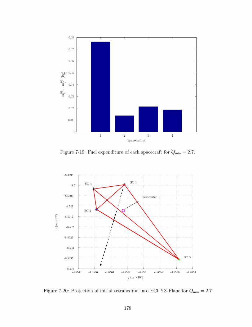
1 2 3 4
m(i
)0
−m
(i)
f(k
g)
0
0.01
0.02
0.03
0.04
0.05
0.06
0.07
0.08
Spacecraft #
Figure 7-19: Fuel expenditure of each spacecraft for Qmin = 2.7.
y (m ×107)
z(m
×106
)
SC 1
SC 2
SC 3
SC 4
mesocenter
-4.8568 -4.8566 -4.8564 -4.8562 -4.856 -4.8558 -4.8556 -4.8554-8.504
-8.5035
-8.503
-8.5025
-8.502
-8.5015
-8.501
-8.5005
-8.5
-8.4995
Figure 7-20: Projection of initial tetrahedron into ECI YZ-Plane for Qmin = 2.7
178

Table 7.3: Phase durations (in minutes) for Qmin = 2.7SC num Burn1 Coast1 Burn2 Coast2 Burn3 Coast3 Coast ROI
1 0 158.483 0 355.017 6.224 61.533 837.3002 1.118 226.667 0 164.500 0 188.967 837.3003 0 157.483 0 84.083 1.746 337.950 837.3004 0.383 272.717 1.143 75.000 0 232.017 837.300
y (m ×107)
z(m
×106
)
SC 1
SC 2
SC 3
SC 4
mesocenter
-5.1338 -5.1336 -5.1334 -5.1332 -5.133 -5.1328 -5.1326-9.001
-9
-8.999
-8.998
-8.997
-8.996
-8.995
-8.994
-8.993
Figure 7-21: Projection of terminal tetrahedron into ECI YZ-Plane for Qmin = 2.7
interest. Note that the constraint on the quality factor becomes active twice during the
region of interest, once at the terminal point and once in the middle of the region of interest.
Interestingly, as seen in Figs. 7-22 and 7-23, the instant of time near the middle of the region
of interest where the quality factor attains is lower bound occurs when the average length
has simultaneously attained its minimum value. When the spacecraft are in close proximity,
small changes in relative position can lead to large changes in the relative geometry. As a
result, the sensitivity of the shape of the tetrahedron to changes in average length is highest
when the spacecraft are more closely spaced. In particular, this sensitivity can result in a
rapid degradation of the quality factor. Fig. 7-24 supports this by showing that the sensitivity
of the quality factor with respect to the average length, ∂Qgm/∂L, is indeed largest at the
179

3 4 5 6 7 8 9
2.7
2.75
2.8
2.85
2.9
2.95
t (s ×104)
Qgm
Figure 7-22: Quality factor in region of interest for Qmin = 2.7
time that L is at a minimum.
Finally, it is observed from Fig. 7-23 that the average length always remains between its
upper and lower bound in the region of interest. A possible explanation why the average
length never attains its lower bound is because of the shape of the tetrahedron is highly
sensitive to changes in L when the average length is small. As a result, it may be difficult to
maintain the quality factor if L is too small. A possible explanation as to why the average
length never attains its upper bound is that an exceedingly large value of L may result in an
increase in fuel consumption (since the initial tetrahedron, while deformed, has an acceptable
average side length only of 9.054 km). As a result, a tetrahedron with a large average length
would not be fuel-optimal.
7.12.2 Ensuring Future Satisfaction of Quality Factor Constraint
It is important to note that the fuel-optimal solution described in Section 7.12.1 does not
consider any potential degradation in the quality factor beyond a single passage though the
180

3 5 6 7 8 9
t (s ×104)
0.4
0.6
0.8
1
1.2
1.4
1.6
1.8
L(m
×104
)
Figure 7-23: Average length, L, in region of interest for Qmin = 2.7
2.7
2.75
2.8
2.85
2.9
2.95
0.95 1 1.05 1.15 1.251.1 1.2
Qgm
Maximum Slope
Enter ROI
Exit ROI
L (m ×104)
Figure 7-24: Quality factor, Qgm, as a function of average length, L, in region of interest forQmin = 2.7. Note: slope of Qgm attains a maximum when L attains a minimum.
181

region of interest. However, if no more maneuvers were performed after the spacecraft have
exited the region of interest, it is clear that perturbations (e.g., oblateness, solar, lunar, and
drag) could potentially degrade the quality of the tetrahedron. As a result, at a future time,
the quality of the formation would be unacceptable.
As an example of potentially unacceptable degradation in the quality of the formation,
suppose that, upon the first exit from the region of interest, it is required that no maneuvers
be performed for a period of three weeks in order to take meausurements without interrup-
tion. Naturally, the tetrahedron must be able to maintain a quality factor of greater than 2.7
during every passage through the region of interest for this three-week period. A question
that arises then is whether an optimal trajectory (such as that obtained in Section 7.12.1)
meets these requirements. Fig. 7-25 shows the trajectory obtained when the final state of
the optimal trajectory of Section 7.12.1 is propagated forward over a period of three weeks.2
It is seen from Fig. 7-25 that the quality of the tetrahedron begins to degrade in the region
of interest on subsequent revolutions. More specifically, it is seen in Fig. 7-25 that, within
20 revolutions (1 revolution ≈ 1 day), the quality of the tetrahedral formation no longer
satisfies the requirement on the quality factor in the region of interest. However, it is noted
that the average side length between the spacecraft changes very little (Fig. 7-26) over this
three-week period, due in large part to the constraint of Eq. 7.30 on the semi-major axis.
Ideally, the way to ensure that the quality factor constraint is met for a specified time into
the future would be to pose an optimal control problem that includes a sufficient number
of revolutions of the orbit and enforces the quality factor constraint during the region of
interest in every revolution. However, this is computationally cumbersome since the size of
the optimal control problem would increase substantially. An alternative to solving such a
complex optimal control problem is to include some margin in the quality factor constraint
for the single revolution optimal control problem (i.e., the problem considered in this section).
In particular, it may be useful to set the lower bound on Qgm to a value that is higher than
the desired value of 2.7 and see if the tetrahedron is of acceptable quality for three-weeks
into the future.
2The three-week propagation was performed using the orbit propagation tool FreeFlyer using oblateness,solar, lunar, and drag perturbations.
182
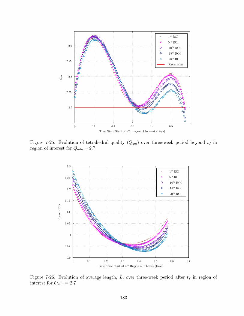
0
2.7
2.75
2.8
2.85
2.9
Qgm
Maxim
0.1 0.2 0.3 0.4 0.5
1st ROI
5th ROI
10th ROI
15th ROI
20th ROI
Constraint
Time Since Start of nth Region of Interest (Days)
Figure 7-25: Evolution of tetrahedral quality (Qgm) over three-week period beyond tf inregion of interest for Qmin = 2.7
00.9
0.95
1
1.05
1.15
1.25
1.1
1.2
1.3
L(m
×104
)
0.1 0.2 0.3 0.4 0.5 0.6 0.7
1st ROI
5th ROI
10th ROI
15th ROI
20th ROI
Time Since Start of nth Region of Interest (Days)
Figure 7-26: Evolution of average length, L, over three-week period after tf in region ofinterest for Qmin = 2.7
183
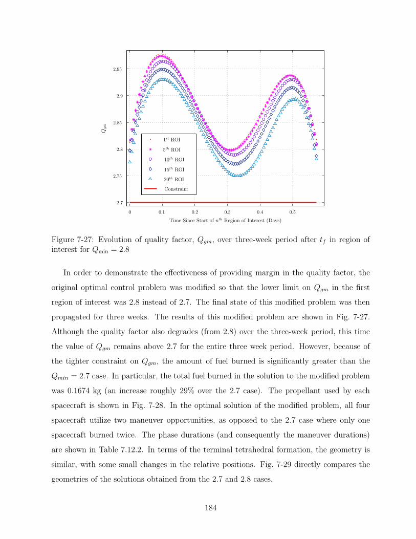
0
2.7
2.75
2.8
2.85
2.9
2.95
Qgm
0.1 0.2 0.3 0.4 0.5
1st ROI
5th ROI
10th ROI
15th ROI
20th ROI
Constraint
Time Since Start of nth Region of Interest (Days)
Figure 7-27: Evolution of quality factor, Qgm, over three-week period after tf in region ofinterest for Qmin = 2.8
In order to demonstrate the effectiveness of providing margin in the quality factor, the
original optimal control problem was modified so that the lower limit on Qgm in the first
region of interest was 2.8 instead of 2.7. The final state of this modified problem was then
propagated for three weeks. The results of this modified problem are shown in Fig. 7-27.
Although the quality factor also degrades (from 2.8) over the three-week period, this time
the value of Qgm remains above 2.7 for the entire three week period. However, because of
the tighter constraint on Qgm, the amount of fuel burned is significantly greater than the
Qmin = 2.7 case. In particular, the total fuel burned in the solution to the modified problem
was 0.1674 kg (an increase roughly 29% over the 2.7 case). The propellant used by each
spacecraft is shown in Fig. 7-28. In the optimal solution of the modified problem, all four
spacecraft utilize two maneuver opportunities, as opposed to the 2.7 case where only one
spacecraft burned twice. The phase durations (and consequently the maneuver durations)
are shown in Table 7.12.2. In terms of the terminal tetrahedral formation, the geometry is
similar, with some small changes in the relative positions. Fig. 7-29 directly compares the
geometries of the solutions obtained from the 2.7 and 2.8 cases.
184

m(i
)0
−m
(i)
f(k
g)
0
0.01
0.02
0.03
0.04
0.05
0.06
0.07
0.08
0.09
Spacecraft #
1 2 3 4
Figure 7-28: Fuel expenditure of each spacecraft for Qmin = 2.8
x (m ×107)
z(m
×106
)
SC 1
SC 2
SC 3
SC 4
-9.002
-9.001
-9
-8.999
-8.998
-8.997
-8.996
-8.995
-8.994
-8.993
7
2.4055 2.406 2.4065 2.407 2.4075
mesocenters
Qmin = 2.7
Qmin = 2.8
Figure 7-29: Comparison of projection of terminal tetrahedra into ECI XZ-Plane for Qmin =2.7 and Qmin = 2.8
185

Table 7.4: Phase durations (in minutes) for Qmin = 2.8 caseSC num Burn1 Coast1 Burn2 Coast2 Burn3 Coast3 Coast ROI
1 0 149.150 0.065 424.850 7.209 0 837.3002 0 184.517 1.008 241.767 1.107 152.867 837.3003 1.448 155.767 0 88.200 1.556 334.300 837.3004 0 273.000 1.268 87.35 0.024 219.617 837.300
7.13 Summary
The problem of determining minimum-fuel maneuver sequences for a four-spacecraft forma-
tion was considered. The objective was to determine fuel-optimal configuration trajectories
that would transfer a four spacecraft formation from an initial parking orbit to a desired
terminal reference orbit while satisfying particular tetrahedral formation constraints. The
configuration problem was solved numerically using the Gauss pseudospectral method. In
particular, two versions of the minimum-fuel configuration problem were considered. In the
first scenario each spacecraft was given two maneuver opportunities to complete the transfer.
In the second scenario each spacecraft was given only one maneuver opportunity. Optimal
solutions, and the discovery of the fuel-optimal orientation was found for each scenario. In
addition, the first-order optimality conditions (or KKT conditions) obtained from the Gauss
pseudospectral method were shown for a multiple-phase optimal control problem. These
KKT conditions were compared with the optimality conditions obtained by discretizing the
calculus of variations problem via the Gauss pseudospectral method. A mapping between
the KKT multipliers and the HBVP costates was used to determine an estimate of the
optimal control for a four spacecraft formation flying problem. It was found that the con-
trol obtained from the NLP was in excellent agreement with the control estimated by the
discretized HBVP.
In addition, a minimum-fuel trajectory was designed to transfer four spacecraft from a
degraded tetrahedral formation into a tetrahedron that satisfied certain geometric quality
constraints for a portion of its orbit. This problem was posed as an optimal control problem
and was solved via direct transcription using the Gauss pseudospectral method. The final
state of the solution was propagated three weeks into the future to examine the potential
186

degradation of the formation. Observing that the formation degraded in an unacceptably
short period of time, a modified optimal control problem was posed that provided margin
in the quality factor. It was found that the solution to this modified problem satisfied the
tetrahedral quality constraints for this entire three week period beyond the final time of
the trajectory design. The results in this chapter provide insight into the relative motion
of tetrahedral formations and demonstrate the applicability of the Gauss pseudospectral
method to spacecraft formation flying problems.
187

[This page intentionally left blank.]
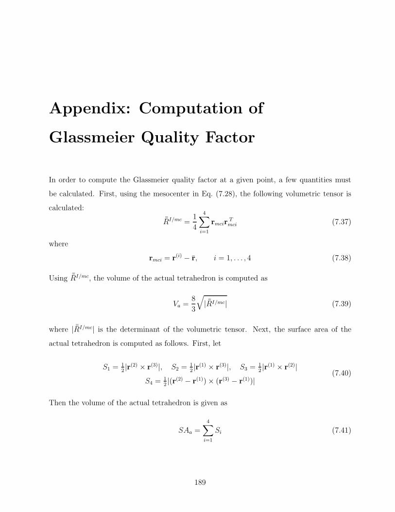
Appendix: Computation of
Glassmeier Quality Factor
In order to compute the Glassmeier quality factor at a given point, a few quantities must
be calculated. First, using the mesocenter in Eq. (7.28), the following volumetric tensor is
calculated:
¯RI/mc =1
4
4∑
i=1
rmcirTmci (7.37)
where
rmci = r(i) − r, i = 1, . . . , 4 (7.38)
Using ¯RI/mc, the volume of the actual tetrahedron is computed as
Va =8
3
√
| ¯RI/mc| (7.39)
where | ¯RI/mc| is the determinant of the volumetric tensor. Next, the surface area of the
actual tetrahedron is computed as follows. First, let
S1 = 12|r(2) × r(3)|, S2 = 1
2|r(1) × r(3)|, S3 = 1
2|r(1) × r(2)|
S4 = 12|(r(2) − r(1)) × (r(3) − r(1))|
(7.40)
Then the volume of the actual tetrahedron is given as
SAa =4∑
i=1
Si (7.41)
189

Lastly, the ideal volume and surface area equations are solely a function of the average side
length, and are expressed below.
V ∗ =
√2
12(L)3, SA∗ =
√3(L)2 (7.42)
190
Chapter 8
Conclusions
This chapter provides a brief recap of the key contributions of this thesis, and expounds on
potential areas for future work.
8.1 Thesis Summary
The Gauss pseudospectral method, a recently developed direct transcription method for
solving optimal control problems, is presented in its most current form. This formulation
has been modified from the original formulation in Ref. 6 by increasing its applicability
to problems with path constraints, explicitly including the terminal state in the NLP, and
improving the control estimate at the boundaries. The Gauss pseudospectral method is
implemented as a global approach, meaning the trajectory is approximated using a global
interpolating polynomial across the entire interval, as opposed to using piecewise polynomials
to locally approximate segments of the trajectory. However, since both implementations can
be found in the literature for pseudospectral methods, a rigorous analytic and numerical
comparison is conducted where the GPM is implemented in both a global and local fashion
on several problems. The results validate the use of a global approach (or semi-global
approach in the presence of known discontinuities).
A comparison is made between three commonly used pseudospectral methods: the Leg-
endre, Radau, and Gauss pseudospectral methods. In order to provide a fair comparison, the
NLP solver SNOPT45 is used for each of the discretizations. Furthermore, all three methods
191

are implemented using the same version of MATLAB R© and the initial guesses provided for
all examples are identical. The accuracy and and computational performance between all
the three methods is compared, and a guideline is created to help determine under what
circumstances each method is appropriate.
This thesis also provides a discussion on past and present attempts to prove the conver-
gence of the NLP solution towards the exact optimal solution as the number of discretization
points increases towards infinity.
Lastly, this thesis applies the Gauss pseudospectral method to tetrahedral spacecraft
formation flying problems. Both orbit insertion problems and reconfiguration problems are
formulated, solved, and analyzed, thus creating a greater understanding for the relative
motion and maneuvers of minimum-fuel spacecraft formations.
8.2 Future Work
This work primarily focuses on the viability of the Gauss pseudospectral method as a pre-
ferred numerical method for solving optimal control problems. Specifically, the GPM’s ca-
pability to obtain accurate, efficient solutions to very complex, non-intuitive problems is
scrutinized, improved, and compared against several other competitive methods. Yet more
advancements can be made to advance the GPM even further. This section will highlight
some of the potential areas where the GPM can be improved.
Real-Time Path Planning
Real-time path planning is one of the hottest topics in this field right now. Simply deter-
mining an optimal trajectory a priori, and then implementing a controller that will bring
the vehicle back to this optimal trajectory in the presence of disturbances has been done
several times and in fact is sub-optimal. Researchers are now looking at control algorithms
that attempt to re-optimize the trajectory once a vehicle deviates from the original optimal
trajectory. Thus the ability to formulate and solve an optimal control problem in real-time
is highly desirable. Simplified optimal control problems, like those that form linear programs
when discretized, have already been used in real-time control. However, there is still much
192

work to be done in terms of implementing nonlinear programs that can be consistently and
reliably solved in real-time. That said, pseudospectral methods have the potential to be
used in real-time due to the extremely high solution accuracy obtained with relatively few
nodes (meaning a smaller problem size). Ross98 has initiated work in real-time optimization
using pseudospectral methods and it is likely others will follow his example. Along similar
lines, research is underway1 to try and reduce the computational burden of pseudospectral
methods. Many real-time applications have a nonconvex feasible region, meaning it may be
quite difficult (or computationally expensive) to start from an arbitrary initial guess and
converge to the globally optimal solution. Research on algorithms that help determine the
initial guess for the GPM transcription may significantly reduce overall computation times
and bring pseudospectral methods closer to real-time applications.
Convergence
As mentioned in Chapter 3, the issue of convergence for the Gauss pseudospectral methods,
and pseudospectral methods in general, is currently unresolved. Due to the global nature
of pseudospectral methods, this proof is inherently different than many convergence proofs
of direct transcription methods. Moreover, the inclusion of a cost function makes this con-
vergence proof more complicated than those of boundary value problems. Yet the evidence
suggests that a convergence proof is tractable, and that the convergence rate for smooth
problems using the GPM is extremely good.
Mesh Refinement
The high accuracy and convergence rate for the GPM requires the assumption that the prob-
lem is sufficiently smooth. However, many real world problems have either state discontinu-
ities, control discontinuities, or both. Often the number and location of these discontinuities
are unknown. A mesh refinement algorithm that could detect discontinuities (and insert
a phase interface in response), and also determine an appropriate number of discretization
points to use would be extremely helpful, and would significantly increase the effectiveness
of pseudospectral methods.
193
Improving the Control
As was seen in Chapter 4, Pontryagin’s minimum principle was used to create a more accu-
rate estimate of the boundary control. This approach works because the state and costate
approximation are more accurate than the control approximation, not only at the bound-
aries, but at the interior points as well. If this approach was able to improve the control at
the boundaries, it may also be able to improve the control at the interior LG points as well,
or possibly even at arbitrary points between the LG points. This result was also noticed by
Hager,56 who first suggested a posteriori computation of the control. More research must be
done in order to determine to what extent this algorithm should be used when determining
the most accurate control profile.
194

Bibliography
1Aoude, G., and How, J., ”Two-Stage path Planning Approach for Designing Multiple
Spacecraft Reconfiguration Maneuvers,” to appear at the 20th International Symposium
on Space Flight Dynamics, Sept, 2007.
2Ascher, U., Mattheij, R., Russel, R., Numerical Solution of Boundary Value Problems for
Ordinary Differential Equations, SIAM-Philadelphia, 1995.
3Athans, M., and Falb, P. L., Optimal Control, McGraw-Hill, New York, 1966, pp. 284-351.
4Axelsson, O., “Global Integration of Differential Equations Through Lobatto Quadra-
ture,” BIT, Vol. 4 (1964) pp. 69-86
5Battin, R.H., An Introduction to the Mathematics and Methods of Astrodynamics, AIAA
Press, New York, 1987, pp. 490-493 and p. 119.
6Benson, D., A Gauss Pseudospectral Transcription for Optimal Control, Ph.D. Disserta-
tion, Department of Aeronautics and Astronautics, Massachusetts Institute of Technology,
November 2004.
7Benson, D.A., Huntington, G.T., Thorvaldsen, T.P., and Rao, A.V., “Direct Trajectory
Optimization and Costate Estimation via an Orthogonal Collocation Method,” AIAA
Guidance, Navigation, and Control Conference, AIAA Paper 2006–6358, Keystone, Col-
orado, August 21–24, 2006.
8Benson, D.A., Huntington, G.T., Thorvaldsen, T.P., and Rao, A.V., “Direct Trajectory
Optimization and Costate Estimation via an Orthogonal Collocation Method,” Journal of
195

Guidance, Control, and Dynamics, Vol. 29, No. 6, November–December 2006, pp. 1435–
1440.
9Bertsekas, D., Nonlinear Programming, Athena Scientific, Belmont, MA,1995.
10Betts, J.T. and Frank, P.D., “A Sparse Nonlinear Optimization Algorithm,” Journal of
Optimization Theory and Applications, Vol. 82, pp. 519-541, 1994.
11Betts, J.T. and Huffman, W.P., “Sparse Optimal Control Software - SOCS,” Mathematics
and Engineering Analysis Library Report, MEA-LR-085, Boeing Information and Support
Services, P. O. Box 3797, Seattle, WA, 98124-2297, 15 July 1997.
12Betts, J.T., “Survey of Numerical Methods for Trajectory Optimization,” Journal of
Guidance, Control, and Dynamics, Vol. 21, No. 2, 1998, pp. 193–207.
13Betts, J.T., “A Direct Approach to Solving Optimal Control Problems,” Computing in
Science and Engineering , May-June 1999, pp. 73-75
14Betts, J.T., Practical Methods for Optimal Control Using Nonlinear Programming, Society
for Industrial and Applied Mathematics Press, 2001.
15Betts, J., Biehn, N., and Campbell, S., ”Convergence of Nonconvergent IRK Discretiza-
tions of Optimal Control Problems with State Inequality Constraints,” SIAM Journal of
Scientific Computing, Vol. 23, No. 6, 2002, pp. 1981–2007.
16Bock, H.G. and Plitt, K.J., “ A Multiple Shooting Algorithm for Direct Solution of
Optimal Control Problems,” IFAC 9th World Congress, Budapest, Hungary, 1984.
17Breger, L.,et al., ”Distributed Control of Formation Flying Spacecraft Build on OA,”
AIAA Guidance, Nav, & Control Conference, Austin, TX, Aug 2003.
18Breger, L. and How, J., ”Formation Flying Control for the MMS Mission using GVE-
based MPC,” Proceedings of the 2005 IEEE Conference on Control Applications, Aug,
2005.
19Breger, L., How., ”J2-Modified GVE-Based MPC for Formation Flying Spacecraft,” AIAA
Guidance, Navigation, and Control Conference, San Francisco, CA, Aug. 15-18, 2005.
196

20Bryson, A., Ho, Y., Applied Optimal Control, Hemisphere Publishing Co., New York,
1975.
21Bryson, A., ”Optimal Control–1950 to 1985”, IEEE Control Systems Magazine, Vol 16,
Issue 3, June 1996, pp. 26-33
22Bryson, A.E., Dynamic Optimization, Addison Wesley Longman, Menlo Park, CA, 1999,
pp. 105–106.
23Canuto, C., Hussaini, M.Y., Quarteroni, A., Zang, T.A., Spectral Methods in Fluid Dy-
namics, Springer-Verlag, New York, 1988.
24Chobotov, V.A., Ed., Orbital Mechanics, AIAA Press, New York, 1991, p. 18.
25Clemente, D., Atkins, E., ”Optimization of a Tetrahedral Satellite Formation,” AIAA
Guidance, Nav, & Control Conference, Aug 2004.
26Cuthrell, J.E. , and Biegler, L.T., “On the Optimization of DIfferential-Algebraic Process
Systems,” AIChE Journal, Vol.33, No.8, pp.1257-1270, Aug. 1987.
27Cuthrell, J.E. and Biegler, L.T., “Simultaneous Optimization and Solution Methods for
Batch Reactor Control Profiles,” Computers and Chemical Engineering, Vol. 13, Nos. 1/2,
1989, pp.49–62.
28Davis, P., Interpolation & Approximation, Dover Publications, 1975.
29Davis, P., Rabinowitz, P., Methods of Numerical Integration, Academic Press, 1984.
30DeBoor, C., A Practical Guide to Splines, Springer-Verlag, New York, NY, 1978.
31Dontchev, A. L., Hager, W., Veliov, V., ”Second-Order Runge-Kutta Approximations in
Control Constrained Optimal Control,” SIAM Journal on Numerical Analysis, Vol. 38,
No. 1, June 2000, pp. 202-226.
32Euler, L., Elementa Calculi variationum, Originally published in Novi Commentarii
academiae scientiarum Petropolitanae 10, 1766, pp. 51-93
197

33Elnagar, G., Kazemi, M., Razzaghi, M., “The Pseudospectral Legendre Method for Dis-
cretizing Optimal Control Problems,” IEEE Transactions on Automatic Control, Vol. 40,
No. 10, October 1995.
34Elnagar, G.E., and Kazemi, M.A., “Pseudospectral Legendre-based optimal computation
of nonlinear constrained variational problems,” Journal of Computational and Applied
Mathematics, Vol. 88, pp.363-375, 1997.
35Elnagar, G. and Kazemi, M., “Pseudospectral Chebyshev Optimal Control of Constrained
Nonlinear Dynamical Systems,” Computational Optimization and Applications, Vol. 11,
1998, pp. 195–217.
36Engelsone, A., Campbell, S., Betts, J., ”Order of Convergence in the Direct Transcription
Solution of Optimal Control Problems,” Proceedings of the 44th Conference on Decision
and Control, Seville, Spain, Dec., 12-15, 2005.
37Enright, P.J. and Conway, B.A., “Discrete Approximations to Optimal Trajectories Using
Direct Transcription and Nonlinear Programming,” Journal of Guidance, Control, and
Dynamics, Vol. 15, No. 4, 1992, pp. 994–1002.
38Fahroo, F. and Ross, I.M., “A Spectral Patching Method for Direct Trajectory Optimiza-
tion,” Journal of the Astronautical Sciences, Vol. 48, No. 2–3, Apr-Sept 2000, pp.269-286.
39Fahroo, F. and Ross, I.M., “Costate Estimation by a Legendre Pseudospectral Method,”
Journal of Guidance, Control, and Dynamics, Vol. 24, No. 2, March-April 2002, pp. 270-
277.
40Fahroo, F. and Ross, I.M., “Direct Trajectory Optimization by a Chebyshev Pseudospec-
tral Method,” Journal of Guidance, Control, and Dynamics, Vol. 25, No. 1, January-
February 2002, pp. 160–166.
41Fahroo, F. and Ross, I., “Pseudospectral Methods for Infinite Horizon Nonlinear Optimal
Control Problems,” 2005 AIAA Guidance, Navigation, and Control Conference, AIAA
Paper 2005-6076, San Francisco, CA, August 15–18, 2005.
198

42Fahroo, F., Ross, I.M., “On Discrete-Time Optimality Conditions for Pseudospectral
Methods,” AIAA/AAS Astrodynamics Specialist Conference and Exhibit, Keystone, CO,
Aug 2006.
43Fornberg, B., A Practical Guide to Pseudospectral Methods, Cambridge University Press,
1998.
44Gear, G., Numerical Initial Value Problems in Ordinary Differential Equations, Prentice-
Hall, New Jersey, 1971.
45Gill, P.E., Murray, W., and Saunders, M.A., “SNOPT: An SQP Algorithm for Large-
Scale Constrained Optimization,” SIAM Journal on Optimization, Vol. 12, No. 4, 2002,
pp. 979–1006.
46Gill, P.E., Users Guide for SNOPT Version 7, A Fortran Package for Large-Scale Nonlinear
Programming, University of California, San Diego, La Jolla, CA, Sept 04.
47Gim, D. , Alfriend, K., “Criteria for Best Configuration and Sub-optimal Reconfiguration
for MMS Mission,” AAS Spaceflight Mechanics Meeting, Maui, HI, Feb. ,2004.
48Gong, Q., Kang, W., and Ross, I., “A Pseudospectral Method for the Optimal Control of
Constrained Feedback Linearizable Systems”, IEEE Transactions on Automatic Control,
Vol. 51, No. 7, July 2006.
49Gong, Q., Ross, I., Kang, W., and Fahroo, F., “On the Pseudospectral Covector Mapping
Theorem for Nonlinear Optimal Control,” IEEE Conference on Decision and Control, Dec
13-15, 2006.
50Gottlieb, D. and Orszag, S., Numerical Analysis of Spectral Methods: Theory and Appli-
cations, Society for Industrial and Applied Mathematics, 1977.
51Gottlieb, D., ”The Stability of Pseudospectral-Chebyshev Methods,” Mathematics of
Computation, Vol. 36, No. 153, Jan 1981, pp.107-118.
199

52Gottlieb, D., Lustman, L., Tadmor, E., ”Convergence of Spectral Methods for Hyperbolic
Initial-Boundary Value Systems”, SIAM Journal on Numerical Analysis, Vol. 24, No. 3,
June 1987, pp. 532–537.
53Guzman, J., Schiff, C., ”A Preliminary Study for a Tetrahedron Formation: Quality
Factors and Visualization,” AIAA Guid, Nav, & Contr, Conf., 2002
54Guzman, J.J., “Tetrahedron Formation Control,” Journal of the Astronautical Sciences,
Vol. 51, No. 4, 2003, pp. 419–431.
55Hager, W.W., “Rate of Convergence for Discrete Approximations to Unconstrained Con-
trol Problems,” SIAM Journal on Numerical Analysis, Vol. 13, 1976, pp. 449–471.
56Hager, W.W., “Runge-Kutta Methods in Optimal Control and the Transformed Adjoint
System,” Numer. Math., Vol. 87, 2000, pp. 247–282.
57Hargraves, C.R. and Paris, S.W., “Direct Trajectory Optimization Using Nonlinear Pro-
gramming and Collocation,” Journal of Guidance, Control, and Dynamics, Vol. 10, No. 4,
1987, pp. 338-342.
58Herman, A.L. and Conway, B.A., “Direct Optimization Using Collocation Based on High
Order Gauss-Lobatto Quadrature Rules,” Journal of Guidance, Control, and Dynamics,
Vol. 19, No. 3, 1996, pp. 592–599.
59Holmstrom, K., Goran, A.O., and Edvall, M.M., “User’s Guide for TOMLAB/SNOPT,”
TOMLAB Optimization, 5 July 2005.
60Hoskins, A. and Atkins, E., “Spacecraft Formation Optimization with a Multi-Impulse
Design,” Proceedings of the 2005 AIAA Guidance, Navigation, and Control Conference,
AIAA Paper 2005–5835, August 15–18, 2005, San Francisco, CA.
61Haung, W., Heping, M., Sun, W., ”Convergence Analysis of Spectral Collocation Methods
for a Singular Differential Equation,” SIAM Journal of Numerical Analysis, Vol. 41, No.
6, pp. 2333-2349.
200

62Hughes, S.P., “Orbit Design for Phase I and Phase II of the Magnetospheric Multiscale
Mission,” NASA Goddard Flight Center. 2004.
63Hughes, S. ”Formation Tetrahedron Design for Phase 1 of the Magnetospheric Multiscale
Mission,” Flight Dynamics Analysis Branch, NASA Goddard Space Flight Center, 2004.
64Hull, D., “Conversion of Optimal Control Problems into Parameter Optimization Prob-
lems,” AIAA Guidance, Navigation, and Control Conference, San Diego, CA, July 29-31,
1996
65Hull, D.G., Optimal Control Theory for Applications, Springer-Verlag, New York, 2003.
66Huntington, G.T., and Rao, A.V., “Optimal Configuration of Spacecraft Formations via a
Gauss Pseudospectral Method,” AAS Spaceflight Mechanics Meeting, AAS 05-103, Copper
Mountain, CO, Jan 2005.
67Huntington, G.T., Benson, D.A., and Rao, A. V., “Post-Optimality Evaluation and Anal-
ysis of a Formation Flying Problem via a Gauss Pseudospectral Method,” Proceedings
of the 2005 AAS/AIAA Astrodynamics Specialist Conference, AAS Paper 05-339, Lake
Tahoe, California, August 7–11, 2005.
68Huntington, G.T. and Rao, A.V., “Optimal Reconfiguration of a Spacecraft Formation
via a Gauss Pseudospectral Method,” Proceedings of the 2005 AAS/AIAA Astrodynamics
Specialist Conference, AAS Paper 05–338, Lake Tahoe, California, August 7–11, 2005.
69Huntington, G. T. , Benson, D. A., How, J. P., Kanizay, N., Darby, C. L., and Rao,
A. V., “Computation of Boundary Controls Using a Gauss Pseudospectral Method,”
2007 Astrodynamics Specialist Conference, Mackinac Island, Michigan, August 21–24,
to appear.
70Huntington, G. T., Benson, D. A, and Rao, A. V., “Design of Optimal Tetrahedral Space-
craft Formations,” The Journal of the Astronautical Sciences, Vol. 55, No. 2, April–June
2007, to appear.
201

71Kameswaran, S. and Biegler, L.T., “Convergence Rates for Dynamic Optimization Using
Radau Collocation,” SIAM Conference on Optimization, Stockholm, Sweden, 2005.
72Kameswaran, S. and Biegler, L.T., “Convergence Rates for Direct Transcription of Op-
timal Control Problems at Radau Points,” Proceedings of the 2006 American Control
Conference, Minneapolis, Minnesota, June 2006.
73Kirk, D.E., Optimal Control Theory, Prentice-Hall, Englewood Cliffs, NJ, 1970.
74Lewis, F. and Syrmos, V., Optimal Control , John Wiley & Sons, New York, 1995.
75Mailhe, L.M. and Guzman, J.J., “Initialization and Resizing of Formation Flying us-
ing Global and Local Optimization Methods,” Proceedings of the 2004 IEEE Aerospace
Conference, Vol. 1, March 6–13, 2004, pp. 556.
76Matrell, C.A. and Lawton, J.A., “Adjoint Variable Solutions via an Auxiliary Opti-
mization Problem,” Journal of Guidance, Control, and Dynamics, Vol. 18, No. 6, 1995,
pp. 1267–1272.
77MATALB, version 2006a: The Language of Scientific Computing, Mathworks, Natick,
MA, 2006.
78Milam, M., Mushambi, K., Murray, M., ”A New Computational Approach to Real-Time
Trajectory Generation for Constrained Mechanical Systems,” Proceedings of the 39th IEEE
Conference on Decision and Control, Sydney, Australia, Dec., 2000.
79Milam, M., ”Real-Time Optimal Trajectory Generation for Constrained Dynamical Sys-
tems,” Ph.D. Thesis, California Institute of Technology, Pasadena, CA, 2003.
80Oberle, H.J. and Grimm, W., “BNDSCO: A proggram for the numerical solution of
optimal control problems,” Technical Report 515, DFVLR, Hamburg, October 2001.
81Paris, S.W., Riehl, J.P., Sjuaw, W..K., “Enhanced Procedures for Direct Trajectory Op-
timization Using Nonlinear Programming and Implicit Integration,” AIAA/AAS Astro-
dynamics Specialist Conference and Exhibit, Keystone CO, Aug 2006
202

82Pontryagin, L.S., Boltyanskii, V., Gamkrelidze, R., Mischenko, E., The Mathematical
Theory of Optimal Processes. Wiley Interscience, New York City, NY, 1962.
83Quarteroni, A., Zampeiri, E., ”Finite Element Preconditioning for Legendre Spectral Col-
location Approximations to Elliptic Equations and Systems”, SIAM Journal on Numerical
Analysis, Vol. 29, No. 4, Aug. 1992, pp.917-936.
84Rao, A.V. and Clarke, K.A., “Performance Optimization of a Maneuvering Re-entry Vehi-
cle Using a Legendre Pseudospectral Method,” 2002 AIAA Atmospheric Flight Mechanics
Conference, AIAA Paper 2002-4885, Monterey, CA August 5–8, 2002.
85Rao, A.V., “Extension of a Pseudospectral Legendre Method to Non-Sequential Multiple-
Phase Optimal Control Problems”, AIAA Guidance, Navigation, and Control Conference,
AIAA Paper No. 2003-5634, Austin, TX, Aug. 11-14, 2003.
86Rao, A.V., GPOCS: A MATLAB Implementation of the Gauss Pseudospectral Method for
Solving Non-Sequential Multiple-Phase Optimal Control Problems, University of Florida,
2007.
87Reddien, G.W., “Collocation at Gauss Points as a Discretization in Optimal Control,”
SIAM Journal of Control and Optimization, Vol. 17, No. 2, March 1979.
88Robert, P., et.al., ”Tetrahedron Geometric Factors,” Analysis Methods for Multi-
Spacecraft Data (G. Paschmann and P. Daly, eds.), pp. 323-348, Nordwijk, The Nether-
lands: ISSI Report SR-001, ESA Publications Division, 1998.
89Ross, I.M. and Fahroo, F., “A Pseudospectral Transformation of the Covectors of Opti-
mal Control Systems,” Proceedings of the 1st IFAC/IEEE Symposium on Structure and
Control, Prague, Czech Republic, August 2001.
90Ross, I.M., Fahroo, F., ”Convergence of Pseudospectral Discretizations of Optimal Control
Problems,” Proceedings of the 40th IEEE Conference on Decision and Control, Orlando,
FL, Dec. 2001.
203

91Ross, I., King, J., and Fahroo, F., “Designing Optimal Spacecraft Formations,” 2002
AIAA/AAS Astrodynamics Specialist Conference, AIAA Paper 2002-4635, Monterey, CA,
August 5–8, 2002.
92Ross, I.M., and Fahroo, F. , “A Direct Method for Solving Nonsmooth Optimal Control
Problems”, Proceedings of the 2002 World Congress of the International Federation on
Automatic Control, IIAC, Barcelona, July 2002.
93Ross, I. M. and Fahroo, F., “A Perspective on Methods for Trajectory Optimization,”
Proceedings of the AIAA/AAS Astrodynamics Specialist Conference, Montery, CA, August
2002. Invited Paper AIAA 2002-4727.
94Ross, I.M. and Fahroo, F., “Legendre Pseudospectral Approximations of Optimal Control
Problems,” Lecture Notes in Control and Information Sciences, Springer-Verlag, 2003.
95Ross, I.M., and Fahroo, F., “Pseudospectral Knotting Methods for Solving Optimal Con-
trol Problems,” Journal of Guidance, Control, and Dynamics, Vol. 27, No. 3, 2004.
96Ross, I.M. and D’Souza,C., “Hybrid Optimal Control Framework for Mission Planning,”
Journal of Guidance, Control, and Dynamics, Vol. 28,No. 4,July-August 2005.
97Ross, I.M. and Fahroo, F., “Legendre Pseudospectral Approximations of Optimal Control
Problems,” Lecture Notes in Control and Information Sciences, Springer-Verlag, 2003.
98Ross, I.M., Fahroo, F., ”Issues in real-time computation of optimal control,” Journal of
Mantematical and Computer Modeling, Vol. 43, 2006, pp. 1172–1188.
99Rossiter, J.A., Model Predictive Control: A Practical Approach, CRC Press, Boca Raton,
FL, 2003
100Scharf, D.P., Hadaegh, F.Y., and Ploen, S.R., ”A Survey of Spacecraft Formation Flying
Guidance and Control (Part I): Guidance,” Proceedings of the American Control Confer-
ence, Denver, CO, pp. 1733–1739, 2003.
204

101Scharf, D.P., Hadaegh, F.Y., and Ploen, S.R., ”A Survey of Spacecraft Formation Flying
Guidance and Control (Part II): Control,” Proceedings of the American Control Confer-
ence, Boston, MA, pp. 2976–2985, 2004.
102Schwartz, A., “Theory and Implementation of Numerical Methods Based on Runge-Kutta
Integration for Solving Optimal Control Problems,” Ph. D. Thesis, University of Califor-
nia, Berkeley, 1996.
103Seywald, H. and Kumar, R.R., “Method for Automatic Costate Calculation,” Journal of
Guidance, Control, and Dynamics, Vol. 19, No. 6, 1996, pp. 1252–1261.
104Silva-Beard, A., Flores-Tlacuahuac, A., and Arrieta-Camacho, J.J., ”Dynamic Trajectory
Optimization Between Unstable Steady-States of a Class of CSTRs,” Proceedings of the
XII European Symposium on Computer Aided Process Engineering, Jan Van Shijndel
(ed.), Elsevier Sccience Publishing Co., The Hague, Ned, 2002.
105Stanton, S. and Proulx, R., “Optimal Orbital Transfer Using a Legendre Pseudospec-
tral Method,” AAS/AIAA Astrodynamics Specialist Conference, AAS-03-574, Big Sky,
Montana, August 3–7, 2003.
106Stoer, J., Bulirsch, R., Introduction to Numerical Analysis, Springer-Verlag, New York,
1993.
107Stryk, O., “Numerical Solution of Optimal Control Problems by Direct Collocation,”
Optimal Control, ed. R. Bulirsch, A. Miele and J. Stoer, Birkhauser Verlag, Basel, 1993,
pp. 129–143.
108Tadmor, E., ”The Exponential Accuracy of Fourier and Chebyshev Differencing Methods,”
SIAM Journal of Numerical Analysis, Vol. 23, No. 1, Feb 1986, pp. 1–10.
109Teo, K.L., Goh C.J., and Wong, K.H., A Unified Computational Approach to Optimal
Control Problems, Longman Scientific & Technical, 1991.
110Thorvaldsen, T., Proulx, R., and Ross, I. M., “A Fast Accurate Method for Low-Thrust
Trajectory Optimization,” Proceedings of the 16th Space Flight Dynamics Conference,
Pasadena, CA, December 2001.
205
111Tillerson, M., Breger, L., How, J.P., ”Distributed Coordination and Control of Formation
Flying Spacecraft,” American Control Conference, Vol. 2, June 4-6, 2003, pp. 1740-1745.
112Trefethen, L.N., Spectral Methods in MATLAB, SIAM Press, Philadelphia, 2000.
113Tsuda, Y., “Global Optimization of Maneuver Schedule for Multiple Spacecrafts Flying
in Formation,” 55th International Astronautical Congress, Vancouver, Canada, IAC-04-
A.2.01, 2004.
114Vallado, D., Fundamentals of Astrodynamics and Applications, McGraw-Hill, 1997.
115Vasantharajan, S., and Biegler, L.T., “Simultaneous Strategies for Optimization of
Differential-Algebraic Systems with Enforcement of Error Criteria,” Computers and
Chemical Engineering, Vol. 14, No. 10, pp.1083-1100, 1990.
116Villadsen, J., and Michelsen, M., “Solution of differential equation models by polynomial
approximation,” Prentice Hall, New Jersey, 1978.
117Vlassenbroeck, J. and Van Doreen, R., “A Chebyshev Technique for Solving Nonlinear
Optimal Control Problems,” IEEE Transactions on Automatic Control, Vol. 33, No. 4,
1988, pp. 333–340.
118Vlassenbroeck, J., “A Chebyshev Polynomial Method for Optimal Control with State
Constraints,” Automatica, Vol. 24, 1988, pp. 499–506.
119Vlases, W.G., Paris, S.W., Lajoie, R.M., Martens, M.J., and Hargraves, C.R., “Optimal
Trajectories by Implicit Simulation,” Boeing Aerospace and Electronics, Technical Report
WRDC-TR-90-3056, Wright-Patterson Air Force Base, 1990.
120Voigt, R.G., Gottlieb, D., Hussaini, M.Y., (eds.) Spectral Methods for Partial Differential
Equations, SIAM-CBMS, Philadelphia, 1984.
121Von Stryk, O., “User’s Guide for DIRCOL 2.1: A Direct Collocation Method for the
Numerical Solution of Optimal Control Problems,” Technische Universitat Darmstadt,
1999.
206

122Well, K., Graphical Environment for Simulation and Optimization, Department of Opti-
mization, Guidance, and Control, Stuttgart, Germany, 2002.
123Wertz, J.R. and Larsen, W.J., Space Mission Analysis and Design, 3rd Edition, Microcosm
Press, El Segundo, CA and Kluwer Academic Publishers, Dordrecht, The Netherlands,
1999, p. 694.
124Wiesel, W.E., Spaceflight Dynamics, McGraw-Hill Companies, Inc., New York, 1997,
pp. 75-76.
125Willems, J.C., ”1696: The Birth of Optimal Control”, Proceedings of the 35th Conference
on Decision and Control, Kobe, Japan, December 1996.
126Williams, P., “Jacobi Pseudospectral Method for Solving Optimal Control Problems”,
Journal of Guidance, Vol. 27, No. 2,2003
127Williams, P., “A Comparison of Differentiation and Integration Based Direct Transcrip-
tion Methods”, AAS/AIAA Space Flight Mechanics Conference, Copper Mountain, CO,
Jan. 23-27, 2005. Paper AAS 05-128.
128Williams, P., “Hermite-Legendre-Gauss-Lobatto Direct Transcription Methods In Trajec-
tory Optimization,” Advances in the Astronautical Sciences. Vol. 120, Part I, pp. 465-484.
2005
129Williams, P., “A Gauss-Lobatto Quadrature Method For Solving Optimal Control Prob-
lems,” Australia Mathematical Society, ANZIAM J.47, pp.C101-C115, July, 2006.
130Williamson, W.E., “Use of Polynomial Approximations to Calculate Suboptimal Con-
trols,” AIAA J. 9 (1971) 2271 - 2273.
207
Top Related