


Languages
Pages
Legal


Advanced Honors Calculus, I and II
(Fall 2021 and Winter 2022)
Volker Runde
November 19, 2021

Contents
Introduction (2020/21) iv
Introduction (2018/19) v
Introduction (2017/18) vi
List of Symbols vii
1 The Real Number System and Finite-Dimensional Euclidean Space 1
1.1 The Real Line . . . . . . . . . . . . . . . . . . . . . . . . . . . . . . . . . . 1
1.2 Functions . . . . . . . . . . . . . . . . . . . . . . . . . . . . . . . . . . . . 13
1.3 The Euclidean Space RN . . . . . . . . . . . . . . . . . . . . . . . . . . . . 17
1.4 Topology . . . . . . . . . . . . . . . . . . . . . . . . . . . . . . . . . . . . 23
2 Limits and Continuity 39
2.1 Limits of Sequences . . . . . . . . . . . . . . . . . . . . . . . . . . . . . . . 39
2.2 Limits of Functions . . . . . . . . . . . . . . . . . . . . . . . . . . . . . . . 46
2.3 Global Properties of Continuous Functions . . . . . . . . . . . . . . . . . . 49
2.4 Uniform Continuity . . . . . . . . . . . . . . . . . . . . . . . . . . . . . . . 53
3 Differentiation in RN 56
3.1 Differentiation in One Variable: A Review . . . . . . . . . . . . . . . . . . 56
3.2 Partial Derivatives . . . . . . . . . . . . . . . . . . . . . . . . . . . . . . . 60
3.3 Vector Fields . . . . . . . . . . . . . . . . . . . . . . . . . . . . . . . . . . 65
3.4 Total Differentiability . . . . . . . . . . . . . . . . . . . . . . . . . . . . . 68
3.5 Taylor’s Theorem . . . . . . . . . . . . . . . . . . . . . . . . . . . . . . . . 75
3.6 Classification of Stationary Points . . . . . . . . . . . . . . . . . . . . . . 79
4 Integration in RN 86
4.1 Content in RN . . . . . . . . . . . . . . . . . . . . . . . . . . . . . . . . . 86
4.2 The Riemann Integral in RN . . . . . . . . . . . . . . . . . . . . . . . . . 89
i

4.3 Evaluation of Integrals in One Variable: A Review . . . . . . . . . . . . . 102
4.4 Fubini’s Theorem . . . . . . . . . . . . . . . . . . . . . . . . . . . . . . . . 105
4.5 Integration in Polar, Spherical, and Cylindrical Coordinates . . . . . . . . 112
5 The Implicit Function Theorem and Applications 122
5.1 Local Properties of C1-Functions . . . . . . . . . . . . . . . . . . . . . . . 122
5.2 The Implicit Function Theorem . . . . . . . . . . . . . . . . . . . . . . . . 126
5.3 Local Extrema under Constraints . . . . . . . . . . . . . . . . . . . . . . . 133
5.4 Change of Variables . . . . . . . . . . . . . . . . . . . . . . . . . . . . . . 139
6 Curve and Surface Integrals and the Integral Theorems by Green, Gauß,
and Stokes 155
6.1 Curves in RN . . . . . . . . . . . . . . . . . . . . . . . . . . . . . . . . . . 155
6.2 Curve Integrals . . . . . . . . . . . . . . . . . . . . . . . . . . . . . . . . . 165
6.3 Green’s Theorem . . . . . . . . . . . . . . . . . . . . . . . . . . . . . . . . 178
6.4 Surfaces in R3 . . . . . . . . . . . . . . . . . . . . . . . . . . . . . . . . . . 185
6.5 Surface Integrals and Stokes’ Theorem . . . . . . . . . . . . . . . . . . . . 190
6.6 Gauß’ Theorem . . . . . . . . . . . . . . . . . . . . . . . . . . . . . . . . . 196
7 Stokes’ Theorem for Differential Forms 203
7.1 Alternating Multilinear Forms . . . . . . . . . . . . . . . . . . . . . . . . . 203
7.2 Differential Forms . . . . . . . . . . . . . . . . . . . . . . . . . . . . . . . 208
7.3 Integration of Differential Forms . . . . . . . . . . . . . . . . . . . . . . . 215
7.4 Simplices and Chains . . . . . . . . . . . . . . . . . . . . . . . . . . . . . . 218
7.5 Stokes’ Theorem . . . . . . . . . . . . . . . . . . . . . . . . . . . . . . . . 225
8 Infinite Series and Improper Integrals 229
8.1 Infinite Series . . . . . . . . . . . . . . . . . . . . . . . . . . . . . . . . . . 229
8.2 Improper Riemann Integrals . . . . . . . . . . . . . . . . . . . . . . . . . . 242
9 Sequences and Series of Functions 251
9.1 Uniform Convergence . . . . . . . . . . . . . . . . . . . . . . . . . . . . . 251
9.2 Power Series . . . . . . . . . . . . . . . . . . . . . . . . . . . . . . . . . . . 256
9.3 Fourier Series . . . . . . . . . . . . . . . . . . . . . . . . . . . . . . . . . . 265
A Linear Algebra 281
A.1 Linear Maps and Matrices . . . . . . . . . . . . . . . . . . . . . . . . . . . 281
A.2 Determinants . . . . . . . . . . . . . . . . . . . . . . . . . . . . . . . . . . 284
A.3 Eigenvalues . . . . . . . . . . . . . . . . . . . . . . . . . . . . . . . . . . . 287
ii

B Limit Superior and Limit Inferior 291
B.1 The Limit Superior . . . . . . . . . . . . . . . . . . . . . . . . . . . . . . . 291
B.2 The Limit Inferior . . . . . . . . . . . . . . . . . . . . . . . . . . . . . . . 293
Index 294
iii

Introduction (2020/21)
This is the 2020/2021 update of my MATH 217/317 notes. Unlike the previous changes
to these notes, these ones are more substantial:
• All graphics have been reworked and—hopefully—made more intelligible as a result.
• The proof of the Change of Variables Theorem has been moved from Chapter 6 to
Chapter 5, where it fits in better.
• An entirely new Chapter 7 has been inserted, which treats differential forms and puts
the classical integral theorems of Green, Stokes, and Gauß into proper perspective.
• Consequently, the old Chapters 7 and 8 have become Chapters 8 and 9, respectively.
Volker Runde, Edmonton August 30, 2021
iv

Introduction (2018/19)
This is the 2018/2019 update of my MATH 217/317 notes. There are no major revisions,
just minor touch ups.
Volker Runde, Edmonton June 1, 2019
v
Introduction (2017/18)
The present notes are based on the courses MATH 217 and 317 as I taught them in the
academic year 2004/2005 and later, again, in 2016/17 and in 2017/18. It is an updated
(and debugged) version of previous incarnations of these notes. The most distinctive
notion of this version is that it includes exercises. Also, some new material has been
added to Sections 6.3 (on conservative vector fields) and 8.3 (Weierstraß’ Approximation
Theorem).
The notes are not intended replace any of the many textbooks on the subject, but
rather to supplement them by relieving the students from the necessity of taking notes
and thus allowing them to devote their full attention to the lecture.
Of course, the degree of originality conveyed in these notes is (very) limited. In putting
them together, I mostly relied on the following sources:
1. James S. Muldowney, Advanced Calculus Lecture Notes for Mathematics 217–
317. Third Edition. (available online);
2. Robert G. Bartle, The Elements of Real Analysis. Second Edition. Jossey-Bass,
1976;
3. Otto Forster, Analysis 2. Vieweg, 1984;
4. Harro Heuser, Lehrbuch der Analysis, Teil 2. Teubner, 1983.
It ought to be clear that these notes may only be used for educational, non-profit
purposes.
Volker Runde, Edmonton April 1, 2018
vi

List of Symbols
−∞, 1
‖ · ‖, 18
∞, 1
| · |, 10
Br(x0), 20
Br[x0], 20
C, 2
∂S, 30
F, 1
f : A→ B, x 7→ f(x), 13
f−1 : A→ B, 14
f−1(Y ), 13
F[X], 3
f(X), 13
F(X), 2
inf S, 7
int S, 31
L = limx→x0 f(x), 46
N, 2
N0, 14
P(S), 16
Q, 2
R, 1
RN , 17
S1 × · · · × SN , 17
Sr[x0], 29
supS, 7
x · y, 17
x = limn→∞ xn, 39
xnn→∞→ x, 39
xn → x, 39
Z, 3
vii

Chapter 1
The Real Number System and
Finite-Dimensional Euclidean
Space
1.1 The Real Line
What is R?
Intuitively, one can think of R as of a line stretching from −∞ to ∞. Intuition,
however, can be deceptive in mathematics. In order to lay solid foundations for calculus,
we introduce R from an entirely formalistic point of view: we demand from a certain set
that it satisfies the properties that we intuitively expect R to have, and then just define
R to be this set!
What are the properties of R we need to do mathematics? First of all,we should be
able to do arithmetic.
Definition 1.1.1. A field is a set F together with two binary operations + and · satisfying
the following:
(F1) for all x, y ∈ F, we have x+ y ∈ F and x · y ∈ F as well;
(F2) for all x, y ∈ F, we have x+ y = y + x and x · y = y · x (commutativity);
(F3) for all x, y, z ∈ F, we have x + (y + z) = (x + y) + z and x · (y · z) = (x · y) · z(associativity);
(F4) for all x, y, z ∈ F, we have x · (y + z) = x · y + x · z (distributivity);
(F5) there are 0, 1 ∈ F with 0 6= 1 such that for all x ∈ F, we have x+ 0 = x and x · 1 = x
(existence of neutral elements);
1

(F6) for each x ∈ F, there is −x ∈ F such that x + (−x) = 0, and for each x ∈ F \ {0},there is x−1 ∈ F such that x · x−1 = 1 (existence of inverse elements).
Items (F1) to (F6) in Definition 1.1.1 re called the field axioms.
For the sake of simplicity, we use the following shorthand notation:
xy := x · y;
x+ y + z := x+ (y + z);
xyz := x(yz);
x− y := x+ (−y);x
y:= xy−1 (where y 6= 0);
xn := x · · ·x︸ ︷︷ ︸n times
(where n ∈ N);
x0 := 1.
Examples. 1. Q, R, and C are fields.
2. Let F be any field then
F(X) :=
{p
q: p and q are polynomials in X with coefficients in F and q 6= 0
}is a field.
3. Define + and · on {A,B} through the following tables:
+ A B
A A B
B B A
and
· A B
A A A
B A B
This turns {A,B} into a field as is easily verified.
4. Define + and · on {©,♣,♥}:
+ © ♣ ♥
© © ♣ ♥♣ ♣ ♥ ©♥ ♥ © ♣
and
· © ♣ ♥
© © © ©♣ © ♣ ♥♥ © ♥ ♣
This turns {©,♣,♥} into a field as is also routinely verified.
2

5. Let
F[X] := {p : p is a polynomial in X with coefficients in F}.
Then F[X] is not a field because, for instance, X has no multiplicative inverse.
6. Both Z and N are not fields.
There are several properties of a field that are not part of the field axioms, but which,
nevertheless, can easily be deduced from them:
1. The neutral elements 0 and 1 are unique: Suppose that both 01 and 02 are neutral
elements for +. Then we have
01 = 01 + 02, by (F5),
= 02 + 01, by (F2),
= 02, again by (F5).
A similar argument works for 1.
2. The inverses −x and x−1 are uniquely determined by x: Let x 6= 0, and let y, z ∈ Fbe such that xy = xz = 1. Then we have
y = y(xz), by (F5) and (F6),
= (yx)z, by (F3),
= (xy)z, by (F2),
= z(xy), again by (F2),
= z, again by (F5) and (F6).
A similar argument works for −x.
3. x0 = 0 for all x ∈ F.
Proof. We have
x0 = x(0 + 0), by (F5),
= x0 + x0, by (F4).
This implies
0 = x0− x0, by (F6),
= (x0 + x0)− x0,
= x0 + (x0− x0), by (F3),
= x0,
which proves the claim.
3

4. (−x)y = −xy holds for all x, y ∈ F.
Proof. We have
xy + (−x)y = (x− x)y = 0.
Uniqueness of −xy then yields that (−x)y = −xy.
5. For any x, y ∈ F, the identity
(−x)(−y) = −(x(−y)) = −(−xy) = xy
holds.
6. If xy = 0, then x = 0 or y = 0.
Proof. Suppose that x 6= 0, so that x−1 exists. Then we have
y = y(xx−1) = (yx)x−1 = 0,
which proves the claim.
Of course, Definition 1.1.1 is not enough to fully describe R. Hence, we need to take
properties of R into account that are not merely arithmetic anymore:
Definition 1.1.2. An ordered field is a field O together with a subset P with the following
properties:
(O1) for x, y ∈ P , we have x+ y ∈ P as well;
(O2) for x, y ∈ P , we have xy ∈ P , as well;
(O3) for each x ∈ O, exactly one of the following holds:
(i) x ∈ P ;
(ii) x = 0;
(iii) −x ∈ P .
Again, we introduce shorthand notation:
x < y :⇐⇒ y − x ∈ P ;
x > y :⇐⇒ y < x;
x ≤ y :⇐⇒ x < y or x = y;
x ≥ y :⇐⇒ x > y or x = y.
As for the field axioms, there are several properties of ordered fields that are not part
of the order axioms (Definition 1.1.2(O1) to (O3)), but follow from them without too
much trouble:
4
1. x < y and y < z implies x < z.
Proof. If y−x ∈ P and z−y ∈ P , then (O1), implies that z−x = (z−y)+(y−x) ∈ Pas well.
2. If x < y, then x+ z < y + z for any z ∈ O.
Proof. This holds because (y + z)− (x+ z) = y − x ∈ P .
3. x < y and z < u implies that x+ z < y + u.
4. x < y and t > 0 implies tx < ty.
Proof. We have ty − tx = t(y − x) ∈ P by (O2).
5. 0 ≤ x < y and 0 ≤ t < s implies tx < sy.
6. x < y and t < 0 implies tx > ty.
Proof. We have
tx− ty = t(x− y) = −t(y − x) ∈ P
because −t ∈ P by (O3).
7. x2 > 0 holds for any x 6= 0.
Proof. If x > 0, then x2 > 0 by (O2). Otherwise, −x > 0 must hold by (O3), so
that x2 = (−x)2 > 0 as well.
In particular 1 = 12 > 0.
8. x−1 > 0 for each x > 0.
Proof. This is true because
x−1 = x−1x−1x = (x−1)2x > 0.
holds.
9. 0 < x < y implies y−1 < x−1.
5

Proof. The fact that xy > 0 implies that x−1y−1 = (xy)−1 > 0. It follows that
y−1 = x(x−1y−1) < y(x−1y−1) = x−1
holds as claimed.
Examples. 1. Q and R are ordered.
2. C cannot be ordered.
Proof. Assume that P ⊂ C as in Definition 1.1.2 does exist. We know that 1 ∈ P .
On the other hand, we have −1 = i2 ∈ P , which contradicts (O3).
3. {A,B} cannot be ordered.
Proof. Assume that there is a set P as required by Definition 1.1.2. Since B ∈ Pand A /∈ P , it follows that P = {B}. But this implies A = B+B ∈ P contradicting
(O1).
Similarly, it can be shown that {©,♣,♥} cannot be ordered.
The last two of these examples are just instances of a more general phenomenon:
Proposition 1.1.3. Let O be an ordered field. Then we can identify the subset {1, 1 +
1, 1 + 1 + 1, . . .} of O with N.
Proof. Let n,m ∈ N be such that
1 + · · ·+ 1︸ ︷︷ ︸n times
= 1 + · · ·+ 1︸ ︷︷ ︸m times
.
Without loss of generality, let n ≥ m. Assume that n > m. Then
0 = 1 + · · ·+ 1︸ ︷︷ ︸n times
− 1 + · · ·+ 1︸ ︷︷ ︸m times
= 1 + · · ·+ 1︸ ︷︷ ︸n−m times
> 0
must hold, which is impossible. Hence, we have n = m.
Hence, if O is an ordered field, it contains a copy of the infinite set N and thus has to
be infinite itself. This means that no finite field can be ordered.
Both R and Q satisfy (O1), (O2), and (O3). Hence, (F1) to (F6) combined with (O1),
(O2), and (O3) still do not fully characterize R.
Definition 1.1.4. Let O be an ordered field, and let ∅ 6= S ⊂ O. Then C ∈ O is called:
(a) an upper bound for S if x ≤ C for all x ∈ S (in this case S is called bounded above);
6

(b) a lower bound for S if x ≥ C for all x ∈ S (in this case S is called bounded below).
If S is both bounded above and below, we simply call it bounded.
Example. The set
{q ∈ Q : q ≥ 0 and q2 ≤ 2}
is bounded below (by 0) and above by 2021.
Definition 1.1.5. Let O be an ordered field, and let ∅ 6= S ⊂ O. Then:
(a) an upper bound for S is called the supremum of S (in short: supS) if supS ≤ C for
every upper bound C for S;
(b) a lower bound for S is called the infimum of S (in short: inf S) if inf S ≥ C for every
lower bound C for S.
Remark. It is easy to see that, whenever a set has a supremum or an infimum, then they
are unique.
Example. The set
S := {q ∈ Q : −2 ≤ q < 3}
is bounded such that inf S = −2 and supS = 3. Clearly, −2 is a lower bound for S and
since −2 ∈ S, it must be inf S. Clearly, 3 is an upper bound for S; if r ∈ Q were an upper
bound of S with r < 3, then
1
2(r + 3) >
1
2(r + r) = r
can not be in S anymore whereas
1
2(r + 3) <
1
2(3 + 3) = 3
implies the opposite. Hence, 3 is the supremum of S.
Do infima and suprema always exist in ordered fields? We shall soon see that this is
not the case in Q.
Definition 1.1.6. An ordered field O is called complete if supS exists for every ∅ 6= S ⊂O which is bounded above.
We shall use completeness to define R:
Definition 1.1.7. R is a complete ordered field.
It can be shown that R is the only complete ordered field (see Exercise 1.2.1 below)
even though this is of little relevance for us: the only properties of R we are interested in
are those of a complete ordered field. From now on, we shall therefore rely on Definition
1.1.7 alone when dealing with R.
Here are a few consequences of completeness:
7
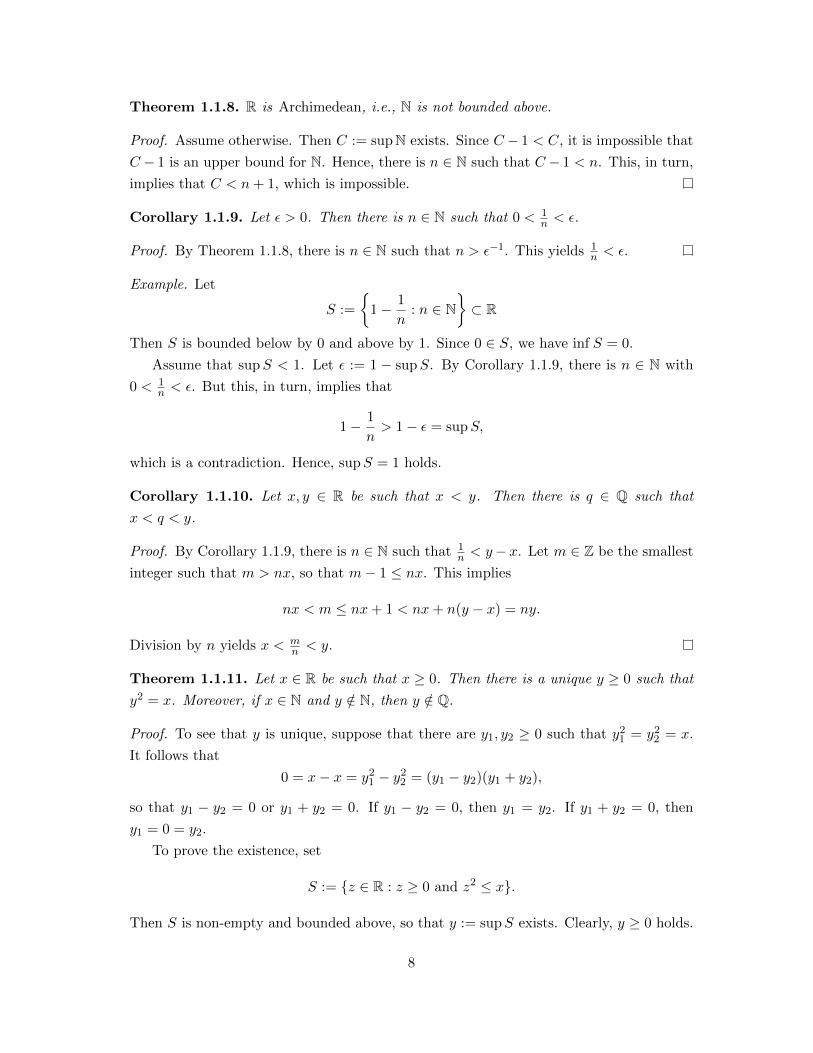
Theorem 1.1.8. R is Archimedean, i.e., N is not bounded above.
Proof. Assume otherwise. Then C := supN exists. Since C − 1 < C, it is impossible that
C − 1 is an upper bound for N. Hence, there is n ∈ N such that C − 1 < n. This, in turn,
implies that C < n+ 1, which is impossible.
Corollary 1.1.9. Let ε > 0. Then there is n ∈ N such that 0 < 1n < ε.
Proof. By Theorem 1.1.8, there is n ∈ N such that n > ε−1. This yields 1n < ε.
Example. Let
S :=
{1− 1
n: n ∈ N
}⊂ R
Then S is bounded below by 0 and above by 1. Since 0 ∈ S, we have inf S = 0.
Assume that supS < 1. Let ε := 1 − supS. By Corollary 1.1.9, there is n ∈ N with
0 < 1n < ε. But this, in turn, implies that
1− 1
n> 1− ε = supS,
which is a contradiction. Hence, supS = 1 holds.
Corollary 1.1.10. Let x, y ∈ R be such that x < y. Then there is q ∈ Q such that
x < q < y.
Proof. By Corollary 1.1.9, there is n ∈ N such that 1n < y− x. Let m ∈ Z be the smallest
integer such that m > nx, so that m− 1 ≤ nx. This implies
nx < m ≤ nx+ 1 < nx+ n(y − x) = ny.
Division by n yields x < mn < y.
Theorem 1.1.11. Let x ∈ R be such that x ≥ 0. Then there is a unique y ≥ 0 such that
y2 = x. Moreover, if x ∈ N and y /∈ N, then y /∈ Q.
Proof. To see that y is unique, suppose that there are y1, y2 ≥ 0 such that y21 = y2
2 = x.
It follows that
0 = x− x = y21 − y2
2 = (y1 − y2)(y1 + y2),
so that y1 − y2 = 0 or y1 + y2 = 0. If y1 − y2 = 0, then y1 = y2. If y1 + y2 = 0, then
y1 = 0 = y2.
To prove the existence, set
S := {z ∈ R : z ≥ 0 and z2 ≤ x}.
Then S is non-empty and bounded above, so that y := supS exists. Clearly, y ≥ 0 holds.
8
We claim that y2 = x.
Assume that y2 < x. Choose n ∈ N such that 1n <
x−y22y+1 . Then(
y +1
n
)2
= y2 +2y
n+
1
n2
≤ y2 +1
n(2y + 1)
< y2 + x− y2
= x
holds, so that y cannot be an upper bound for S. Hence, we have a contradiction, so that
y2 ≥ x must hold.
Assume now that y2 > x. Choose n ∈ N such that 1n <
12y (y2 − x), and note that(
y − 1
n
)2
= y2 − 2y
n+
1
n2
> y2 − 2y
n
> y2 − (y2 − x)
= x
≥ z2
for all z ∈ S. This, in turn, implies that y − 1n ≥ z for all z ∈ S. Hence, y − 1
n < y is an
upper bound for S, which contradicts the definition of supS.
All in all, y2 = x must hold.
Suppose now that x ∈ N, and assume that y ∈ Q \ N. Let m,n ∈ N be such that
y = mn , and suppose without loss of generality that gcd(n,m) = 1. Let p1, . . . , pk and
q1, . . . , q` be each pairwise distinct primes such that
m = pµ11 · · · pµkk and n = qν11 · · · q
ν``
for suitable µ1, . . . , µk, ν1, . . . , ν` ∈ N. As x = y2 = m2
n2 , it follows that
q2ν11 · · · q2ν`
` x = n2x = m2 = p2µ11 · · · p2µk
k .
Uniqueness of the prime factorization of n2x then yields {q1, . . . , q`} ⊂ {p1, . . . , pk}, which
contradicts gcd(m,n) = 1.
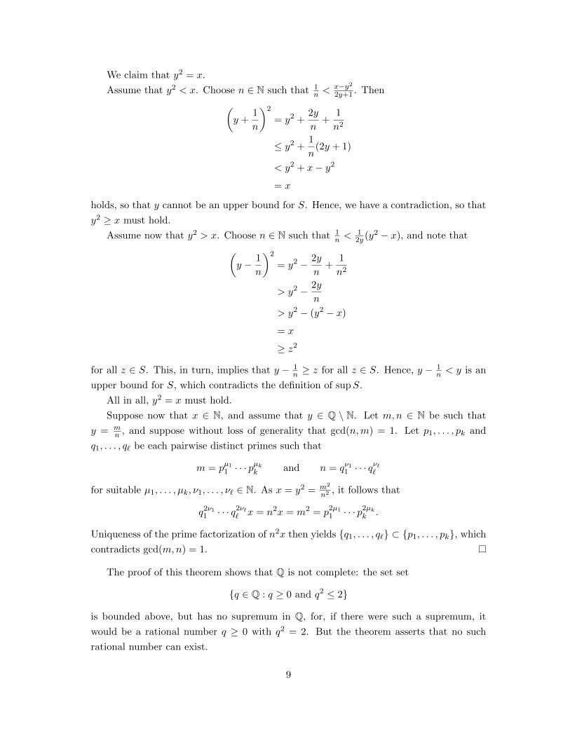
The proof of this theorem shows that Q is not complete: the set set
{q ∈ Q : q ≥ 0 and q2 ≤ 2}
is bounded above, but has no supremum in Q, for, if there were such a supremum, it
would be a rational number q ≥ 0 with q2 = 2. But the theorem asserts that no such
rational number can exist.
9
For a, b ∈ R with a < b, we introduce the following notation:
[a, b] := {x ∈ R : a ≤ x ≤ b} (closed interval );
(a, b) := {x ∈ R : a < x < b} (open interval );
(a, b] := {x ∈ R : a < x ≤ b};
[a, b) := {x ∈ R : a ≤ x < b}.
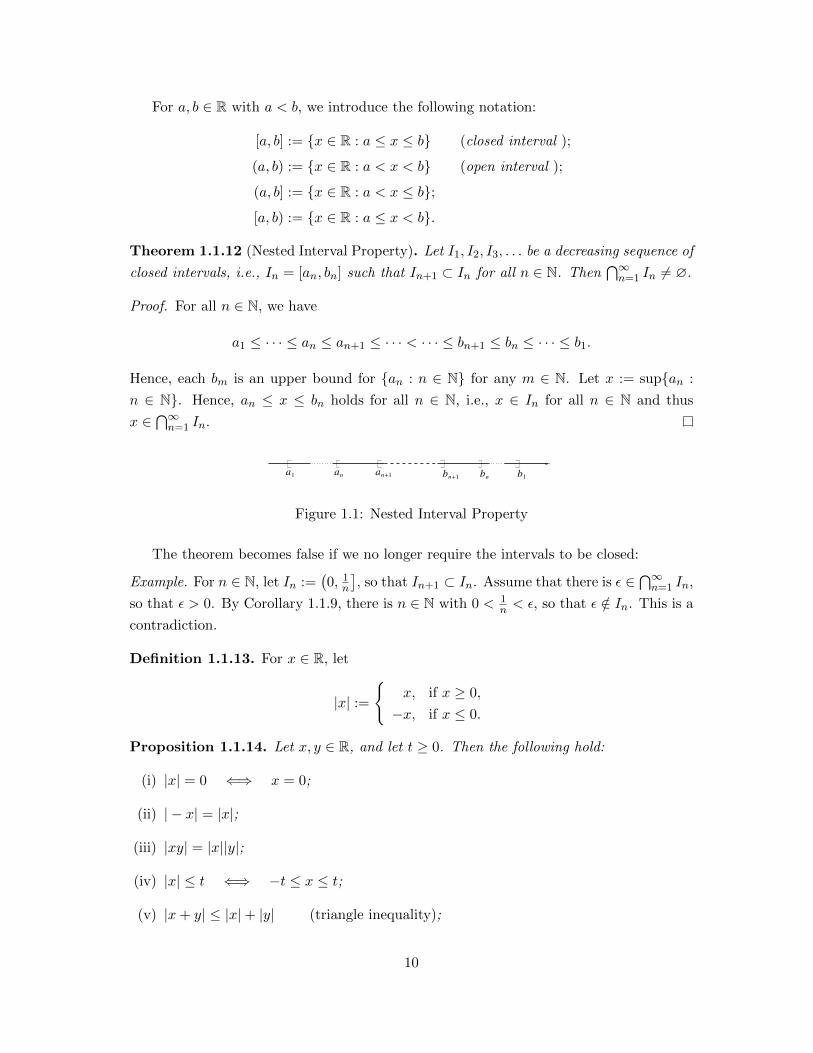
Theorem 1.1.12 (Nested Interval Property). Let I1, I2, I3, . . . be a decreasing sequence of
closed intervals, i.e., In = [an, bn] such that In+1 ⊂ In for all n ∈ N. Then⋂∞n=1 In 6= ∅.
Proof. For all n ∈ N, we have
a1 ≤ · · · ≤ an ≤ an+1 ≤ · · · < · · · ≤ bn+1 ≤ bn ≤ · · · ≤ b1.
Hence, each bm is an upper bound for {an : n ∈ N} for any m ∈ N. Let x := sup{an :
n ∈ N}. Hence, an ≤ x ≤ bn holds for all n ∈ N, i.e., x ∈ In for all n ∈ N and thus
x ∈⋂∞n=1 In.
a1 an n+1an+1b bn b1
Figure 1.1: Nested Interval Property
The theorem becomes false if we no longer require the intervals to be closed:
Example. For n ∈ N, let In :=(0, 1
n
], so that In+1 ⊂ In. Assume that there is ε ∈
⋂∞n=1 In,
so that ε > 0. By Corollary 1.1.9, there is n ∈ N with 0 < 1n < ε, so that ε /∈ In. This is a
contradiction.
Definition 1.1.13. For x ∈ R, let
|x| :=
{x, if x ≥ 0,
−x, if x ≤ 0.
Proposition 1.1.14. Let x, y ∈ R, and let t ≥ 0. Then the following hold:
(i) |x| = 0 ⇐⇒ x = 0;
(ii) | − x| = |x|;
(iii) |xy| = |x||y|;
(iv) |x| ≤ t ⇐⇒ −t ≤ x ≤ t;
(v) |x+ y| ≤ |x|+ |y| (triangle inequality);
10

(vi) ||x| − |y|| ≤ |x− y|.
Proof. (i), (ii), and (iii) are routinely checked.
(iv): Suppose that |x| ≤ t. If x ≥ 0, we have −t ≤ x = |x| ≤ t; for x ≤ 0, we have
−x ≥ 0 and thus −t ≤ −x ≤ t. This implies −t ≤ x ≤ t. Hence, −t ≤ x ≤ t holds for any
x with |x| ≤ t.Conversely, suppose that −t ≤ x ≤ t. For x ≥ 0, this means x = |x| ≤ t. For x ≤ 0,
the inequality −t ≤ x implies that |x| = −x ≤ t.(v): By (iv), we have
−|x| ≤ x ≤ |x| and − |y| ≤ y ≤ |y|.
Adding these two inequalities yields
−(|x|+ |y|) ≤ x+ y ≤ |x|+ |y|.
Again by (iv), we obtain |x+ y| ≤ |x|+ |y| as claimed.
(vi): By (v), we have
|x| = |x− y + y| ≤ |x− y|+ |y|
and hence
|x| − |y| ≤ |x− y|.
Exchanging the roles of x and y yields
−(|x| − |y|) = |y| − |x| ≤ |y − x| = |x− y|,
so that
||x| − |y|| ≤ |x− y|
holds by (iv).
Exercises
1. Let + and · be defined on {♠, †,©,A} through:
+ ♠ † © A
♠ ♠ † © A
† † © A ♠© © A ♠ †A A ♠ † ©
· ♠ † © A
♠ ♠ ♠ ♠ ♠† ♠ † © A
© ♠ © ♠ ©A ♠ A © †
.
Do these turn {♠, †,©,A} into a field?
11

2. Show that
Q[√
2]
:={p+ q
√2 : p, q ∈ Q
},
with + and · inherited from R, is a field.
(Hint : Many of the field axioms are true for Q[√
2]
simply because they are true
for R; in this case, just point it out and don’t verify the axiom in detail.)
3. Let O be an ordered field, and let x, y, z, u ∈ O:
(a) suppose that x < y and z < u, and show that x+ z < y + u;
(b) suppose that 0 ≤ x < y and 0 ≤ z < u, and show that xz < yu.
You may use the axioms of an ordered field and all the properties that were derived
from them in class.
4. Let ∅ 6= S ⊂ R be bounded below, and let −S := {−x : x ∈ S}. Show that:
(a) −S is bounded above.
(b) S has an infimum, namely inf S = − sup(−S).
5. Find supS and inf S in R for
S :=
{(−1)n
(1− 1
n
): n ∈ N
}.
Justify, i.e., prove, your findings.
6. Let S, T ⊂ R be non-empty and bounded above. Show that
S + T := {x+ y : x ∈ S, y ∈ T}
is also bounded above with
sup(S + T ) = supS + supT.
7. An ordered field O is said to have the nested interval property if⋂∞n=1 In 6= ∅ for
each decreasing sequence I1 ⊃ I2 ⊃ I3 ⊃ · · · of closed intervals in O.
Show that an Archimedean ordered field with the nested interval property is com-
plete.
8. Let x, y ∈ R with x < y. Show that there is z ∈ R \Q such that x < z < y.
12
1.2 Functions
In this section, we give a somewhat formal introduction to functions and introduce the
notions of injectivity, surjectivity, and bijectivity. We use bijective maps to define what
it means for two (possibly infinite) sets to be “of the same size” and show that N and Qhave “the same size” whereas R is “larger” than Q.
Definition 1.2.1. Let A and B be non-empty sets. A subset f of
A×B := {(a, b) : a ∈ A, b ∈ B}
is called a function, mapping map if, for each x ∈ A, there is a unique y ∈ B such that
(x, y) ∈ f .
For a function f ⊂ A×B, we write f : A→ B and, for (x, y) ∈ A×B,
y = f(x) :⇐⇒ (x, y) ∈ f.
We then often write
f : A→ B, x 7→ f(x).
The set A is called the domain of of f , and B is called its co-domain.
Definition 1.2.2. Let A and B be non-empty sets, let f : A→ B be a function, and let
X ⊂ A and Y ⊂ B. Then
f(X) := {f(x) : x ∈ X} ⊂ B
is the image of X (under f), and
f−1(Y ) := {x ∈ A : f(x) ∈ Y } ⊂ A
is the inverse!image of Y (under f). The set f(A) is called the range of f .
Example. Consider sin : R→ R, i.e., {(x, sin(x)) : x ∈ R} ⊂ R× R. Then we have:
sin(R) = [−1, 1];
sin([0, π]) = [0, 1];
sin−1({0}) = {nπ : n ∈ Z};
sin−1({x ∈ R : x ≥ 7}) = ∅.
Definition 1.2.3. Let A and B be non-empty sets, and let f : A → B be a function.
Then f is called:
(a) injective if f(x1) 6= f(x2) whenever x1 6= x2 for x1, x2 ∈ A;
13

(b) surjective if f(A) = B;
(c) bijective if it is both injective and surjective.
Examples. 1. The function
f1 : R→ R, x 7→ x2
is neither injective nor surjective, whereas
f2 : [0,∞)︸ ︷︷ ︸:={x∈R:x≥0}
→ R, x 7→ x2
is injective, but not surjective, and
f3 : [0,∞)→ [0,∞), x 7→ x2
is bijective.
2. The function
sin : [0, 2π]→ [−1, 1], x 7→ sin(x)
is surjective, but not injective.
Remark. If f : A→ B is bijective, the map
B → A, f(x)→ x
is well defined and called the inverse map and denoted by f−1 : A→ B.
For finite sets, it is obvious what it means for two sets to have the same size or for
one of them to be smaller or larger than the other one. For infinite sets, matters are more
complicated:
Example. Let N0 := N ∪ {0}. Then N is a proper subset of N0, so that N should be
“smaller” than N0. On the other hand,
N0 → N, n 7→ n+ 1
is bijective, i.e., there is a one-to-one correspondence between the elements of N0 and N.
Hence, N0 and N should “have the same size”.
We use the second idea from the previous example to define what it means for two
sets to have “the same size”:
Definition 1.2.4. Two sets A and B are said to have the same cardinality—in symbols:
|A| = |B|—if there is a bijective map f : A→ B.
Examples. 1. If A and B are finite, then |A| = |B| holds if and only if A and B have
the same number of elements.
14

2. By the previous example, we have |N| = |N0|—even though N is a proper subset of
N0.
3. The function
f : N→ Z, n 7→ (−1)n⌊n
2
⌋is bijective, so that we can enumerate Z as {0, 1,−1, 2,−2, . . .}. As a consequence,
|N| = |Z| holds even though N ( Z.
4. Let a1, a2, a3, . . . be an enumeration of Z. We can then write Q as a rectangular
scheme that allows us to enumerate Q. Omitting duplicates, we conclude that
|Q| = |N|:
a1 a2 a3 a4 a5
a2
2
a3
2
a4
2
a5
2
a1
2
1
3
a2
3
a3
3
a4
3
a5
3
a1
4
a2
4
a3
4
a4
4
a5
4
a1
5
a2
5
a3
5
a4
5
a5
5
a
Figure 1.2: Enumeration of Q
5. Let a < b. The function
f : [a, b]→ [0, 1], x 7→ x− ab− a
is bijective, so that |[a, b]| = |[0, 1]|.
Definition 1.2.5. A set A is called countable if it is finite or if |A| = |N|.
A set A is countable, if and only if we can enumerate it, i.e., A = {a1, a2, a3, . . .} where
the sequence a1, a2, a3, . . . may break off after a finite number of terms.
As we have already seen, the sets N, N0, Z, and Q are all countable. But not all sets
are:
15

Theorem 1.2.6. The sets [0, 1] and R are not countable.
Proof. We only consider [0, 1] (this is enough because it is easy to see that a an infinite
subsets of a countable set must again be countable).
Each x ∈ [0, 1] has a decimal expansion
x = 0.ε1ε2ε3 · · · (1.1)
with ε1, ε2, ε3, . . . ∈ {0, 1, 2, . . . , 9}.Assume that there is an enumeration [0, 1] = {a1, a2, a3, . . .}. Define x ∈ [0, 1] using
(1.1) by letting, for n ∈ N,
εn :=
{6, if the n-th digit of an is 7,
7, if the n-th digit of an is not 7
Let n ∈ N be such that x = an.
Case 1: The n-th digit of an is 7. Then the n-th digit of x is 6, so that an 6= x.
Case 2: The n-th digit of an is not 7. Then the n-th digit of x is 7, so that an 6= x,
too.
Hence, x /∈ {a1, a2, a3, . . .}, which contradicts [0, 1] = {a1, a2, a3, . . .}.
The argument used in the proof of Theorem 1.2.6 is called Cantor’s Diagonal Argu-
ment.
Exercises
1. Let R be a complete ordered field, and let ι0 : Q → R be the canonical embedding.
Show that
ι : R→ R, x 7→ sup{ι0(q) : q ∈ Q, q ≤ x}
defines a bijective map satisfying:
• ι(x+ y) = ι(x) + ι(y) for x, y ∈ R;
• ι(xy) = ι(x)ι(y) for x, y ∈ R;
• ι(x) > 0 if x > 0.
2. For any set S, its power set P(S) is defined to be the set consisting of all subsets of
S. Show that there is no surjective map from S to P(S). (Hint : Assume that there
is a surjective map f : S → P(S) and consider the set {x ∈ S : x /∈ f(x)}.)
16

1.3 The Euclidean Space RN
Recall that, for any sets S1, . . . , SN , their (N -fold) Cartesian product is defined as
S1 × · · · × SN := {(s1, . . . , sN ) : sj ∈ Sj for j = 1, . . . , N}.
The N -dimensional Euclidean space is defined as
RN := R× · · · × R︸ ︷︷ ︸N times
= {(x1, . . . , xN ) : x1, . . . , xN ∈ R}.
An element x := (x1, . . . , xN ) ∈ RN is called a point or vector in RN ; the real numbers
x1, . . . , xN ∈ R are the coordinates of x. The vector 0 := (0, . . . , 0) is the origin or zero
vector of RN . (For N = 2 and N = 3, the space RN can be identified with the plane and
three-dimensional space of geometric intuition.)
We can add vectors in RN and multiply them with real numbers: For two vectors
x = (x1, . . . , xN ), y := (y1, . . . , yN ) ∈ RN and a scalar λ ∈ R define:
x+ y := (x1 + y1, . . . , xN + yN ) (addition);
λx := (λx1, . . . , λxN ) (scalar multiplication).
The following rules for addition and scalar multiplication in RN are easily verified:
x+ y = y + x;
(x+ y) + z = x+ (y + z);
0 + x = x;
x+ (−1)x = 0;
1x = x;
0x = 0;
λ(µx) = (λµ)x;
λ(x+ y) = λx+ λy;
(λ+ µ)x = λx+ µx.
This means that RN is a vector space.
Definition 1.3.1. The inner product on RN is defined by
x · y :=N∑j=1
xjyj
for x = (x1, . . . , xN ), y := (y1, . . . , yN ) ∈ RN .
Proposition 1.3.2. The following hold for all x, y, z ∈ RN and λ ∈ R:
17
(i) x · x ≥ 0;
(ii) x · x = 0 ⇐⇒ x = 0;
(iii) x · y = y · x;
(iv) x · (y + z) = x · y + x · z;
(v) (λx) · y = λ(x · y) = x · λy.
Definition 1.3.3. The (Euclidean) norm on RN is defined by
‖x‖ :=√x · x =
√√√√ N∑j=1
x2j
for x = (x1, . . . , xN ).
For N = 2, 3, the norm ‖x‖ of a vector x ∈ RN can be interpreted as its length. The
Euclidean norm on RN thus extends the notion of length in 2- and 3-dimensional space,
respectively, to arbitrary dimensions.
Lemma 1.3.4 (Geometric versus Arithmetic Mean). For x, y ≥ 0, the inequality
√xy ≤ 1
2(x+ y)
holds with equality if and only if x = y.
Proof. We have
x2 − 2xy + y2 = (x− y)2 ≥ 0 (1.2)
with equality if and only if x = y. This yields
xy ≤ xy +1
4(x2 − 2xy + y2) (1.3)
= xy +1
4x2 − 1
2xy +
1
4y2
=1
4x2 +
1
2xy +
1
4y2
=1
4(x2 + 2xy + y2)
=1
4(x+ y)2.
Taking roots yields the desired inequality. It is clear that we have equality if and only if
the second summand in (1.3) vanishes; by (1.2) this is possible only if x = y.
18

Theorem 1.3.5 (Cauchy–Schwarz Inequality). We have
|x · y| ≤N∑j=1
|xjyj | ≤ ‖x‖‖y‖
for x = (x1, . . . , xN ), y := (y1, . . . , yN ) ∈ RN .
Proof. The first inequality is clear due to the triangle inequality in R.
If ‖x‖ = 0, then x1 = · · · = xN = 0, so that∑N
j=1 |xjyj | = 0; a similar argument
applies if ‖y‖ = 0. We may therefore suppose that ‖x‖‖y‖ 6= 0. We then obtain
N∑j=1
|xj ||yj |‖x‖‖y‖
=
N∑j=1
√(xj‖x‖
)2( yj‖y‖
)2
≤N∑j=1
1
2
[(xj‖x‖
)2
+
(yj‖y‖
)2], by Lemma 1.3.4,
=1
2
1
‖x‖2N∑j=1
x2j +
1
‖y‖2N∑j=1
y2j
=
1
2
[‖x‖2
‖x‖2+‖y‖2
‖y‖2
]= 1.
Multiplication by ‖x‖‖y‖ yields the claim.
Proposition 1.3.6 (Properties of ‖ · ‖). For x, y ∈ RN and λ ∈ R, we have:
(i) ‖x‖ ≥ 0;
(ii) ‖x‖ = 0 ⇐⇒ x = 0;
(iii) ‖λx‖ = |λ|‖x‖;
(iv) ‖x+ y‖ ≤ ‖x‖+ ‖y‖ (triangle inequality);
(v) |‖x‖ − ‖y‖| ≤ ‖x− y‖.
Proof. (i), (ii), and (iii) are easily verified.
For (iv), note that
‖x+ y‖2 = (x+ y) · (x+ y)
= x · x+ x · y + y · x+ y · y
= ‖x‖2 + 2x · y + ‖y‖2
≤ ‖x‖2 + 2‖x‖‖y‖+ ‖y‖2, by Theorem 1.3.5,
= (‖x‖+ ‖y‖)2.
19

Taking roots yields the claim.
For (v), note that—by (iv) with x and y replaced by x− y and y—
‖x‖ = ‖(x− y) + y‖ ≤ ‖x− y‖+ ‖y‖,
holds, so that
‖x‖ − ‖y‖ ≤ ‖x− y‖.
Interchanging x and y yields
‖y‖ − ‖x‖ ≤ ‖y − x‖ = ‖x− y‖,
so that
−‖x− y‖ ≤ ‖x‖ − ‖y‖ ≤ ‖x− y‖.
This proves (v).
We now use the norm on RN to define two important types of subsets of RN :
Definition 1.3.7. Let x0 ∈ RN and let r > 0. Then:
(a) the open ball in RN centered at x0 with radius r is the set
Br(x0) := {x ∈ RN : ‖x− x0‖ < r}.
(b) the closed ball in RN centered at x0 with radius r is the set
Br[x0] := {x ∈ RN : ‖x− x0‖ ≤ r}.
For N = 1, Br(x0) and Br[x0] are nothing but open and closed intervals, respectively,
namely
Br(x0) = (x0 − r, x0 + r) and Br[x0] = [x0 − r, x0 + r].
Moreover, if a < b, then
(a, b) = (x0 − r, x0 + r) and [a, b] = [x0 − r, x0 + r]
holds, with x0 := 12(a+ b) and r := 1
2(b− a).
For N = 2, Br(x0) and Br[x0] are just disks with center x0 and radius r, where the
circle is not included in the case of Br(x0), but is included for Br[x0].
Finally, if N = 3, then Br(x0) and Br[x0] are balls in the sense of geometric intuition.
In the open case, the surface of the ball is not included, but it is included in the closed
ball.
Definition 1.3.8. A set C ⊂ RN is called convex if tx+ (1− t)y ∈ C for all x, y ∈ C and
t ∈ [0, 1].
20

In plain language, a set is convex if, for any two points x and y in the C, the whole
line segment joining x and y is also in C:
y
x
Figure 1.3: A convex subset of R2
y
x
Figure 1.4: Not a convex subset of R2
Proposition 1.3.9. Let x0 ∈ RN , and let r > 0. Then Br(x0) and Br[x0] are convex.
Proof. We only prove the claim for Br(x0) in detail.
21

Let x, y ∈ Br(x0) and t ∈ [0, 1]. Then we have
‖tx+ (1− t)y − x0‖ = ‖t(x− x0) + (1− t)(y − x0)‖
≤ t‖x− x0‖+ (1− t)‖y − x0‖
< tr + (1− t)r (1.4)
= r,
so that tx+ (1− t)y ∈ Br(x0).
The claim for Br[x0] is proved similarly, but with ≤ instead of < in (1.4).
Let I1, . . . , IN ⊂ R be closed intervals, i.e., Ij = [aj , bj ] where aj < bj for j = 1, . . . , N .
Then I := I1 × · · · × IN is called a closed interval in RN . We have
I = {(x1, . . . , xN ) ∈ RN : aj ≤ xj ≤ bj for j = 1, . . . , N}.
For N = 2, a closed interval in RN , i.e., in the plane, is just a rectangle. For N = 3, a
closed interval in R3 is a rectangular box.
Theorem 1.3.10 (Nested Interval Property in RN ). Let I1, I2, I3, . . . be a decreasing
sequence of closed intervals in RN . Then⋂∞n=1 In 6= ∅ holds.
Proof. Each interval In is of the form
In = In,1 × · · · × In,N
with closed intervals In,1, . . . , In,N in R. For each j = 1, . . . , N , we have
I1,j ⊃ I2,j ⊃ I3,j ⊃ · · · ,
i.e., the sequence I1,j , I2,j , I3,j , . . . is a decreasing sequence of closed intervals in R. By
Theorem 1.1.12, this means that⋂∞n=1 In,j 6= ∅, i.e., there is xj ∈ In,j for all n ∈ N.
Let x := (x1, . . . , xN ). Then x ∈ In,1 × · · · × In,N holds for all n ∈ N, which means that
x ∈⋂∞n=1 In.
Exercises
1. For x = (x1, . . . , xN ) ∈ RN , set
‖x‖1 := |x1|+ · · ·+ |xN | and ‖x‖∞ := max{|x1|, . . . , |xN |}.
(a) Show that the following are true for j = 1,∞, x, y ∈ RN and λ ∈ R:
(i) ‖x‖j ≥ 0 and ‖x‖j = 0 if and only if x = 0;
(ii) ‖λx‖j = |λ|‖x‖j ;
22

(iii) ‖x+ y‖j ≤ ‖x‖j + ‖y‖j .
(b) For N = 2, sketch the sets of those x for which ‖x‖1 ≤ 1, ‖x‖ ≤ 1, and
‖x‖∞ ≤ 1.
(c) Show that
‖x‖1 ≤√N‖x‖ ≤ N ‖x‖∞
for all x ∈ RN .
2. Let x, y ∈ RN . Show that |x · y| = ‖x‖‖y‖ holds if and only if x and y are linearly
dependent.
3. Show that
‖x+ y‖2 = ‖x‖2 + ‖y‖2 ⇐⇒ x · y = 0
for any x, y ∈ RN .
4. Let C be a family of convex sets in RN . Show that⋂C∈C C is again convex. Is⋃
C∈C C necessarily convex?
1.4 Topology
The word topology derives from the Greek and literally means “study of places”. In
mathematics, topology is the discipline that provides the conceptual framework for the
study of continuous functions:
Definition 1.4.1. Let x0 ∈ RN . A set U ⊂ RN is called a neighborhood of x0 if there is
ε > 0 such that Bε(x0) ⊂ U .
��������
��������
x~
0x 0
x 0Bε( )
x
U
Figure 1.5: A neighborhood of x0, but not of x0
Examples. 1. If x0 ∈ RN is arbitrary, and r > 0, then both Br(x0) and Br[x0] are
neighborhoods of x0.
23

2. The interval [a, b] is not a neighborhood of a: To see this assume that is is a
neighborhood of a. Then there is ε > 0 such that
Bε(a) = (a− ε, a+ ε) ⊂ [a, b],
which would mean that a− ε ≥ a. This is a contradiction.
Similarly, [a, b] is not a neighborhood of b, [a, b) is not a neighborhood of a, and
(a, b] is not a neighborhood of b.
Definition 1.4.2. A set U ⊂ RN is open if it is a neighborhood of each of its points.
Examples. 1. ∅ and RN are trivially open.
2. Let x0 ∈ RN , and let r > 0. We claim that Br(x0) is open. Let x ∈ Br(x0). Choose
ε ≤ r − ‖x− x0‖, and let y ∈ Bε(x). It follows that
‖y − x0‖ ≤ ‖y − x‖︸ ︷︷ ︸<ε
+‖x− x0‖
< r − ‖x− x0‖+ ‖x− x0‖
= r;
hence, Bε(x) ⊂ Br(x0) holds.
x 0
Bε
x 0Br )(
x 0|||| x −
r
x
ε
)(x
Figure 1.6: Open balls are open
In particular, (a, b) is open for all a, b ∈ R such that a < b. On the other hand,
[a, b], (a, b], and [a, b) are not open.
24

3. The set
S := {(x, y, z) ∈ R3 : y2 + z2 = 1, x > 0}
is not open.
Proof. Clearly, x0 := (1, 0, 1) ∈ S. Assume that there is ε > 0 such that Bε(x0) ⊂ S.
It follows that (1, 0, 1 +
ε
2
)∈ Bε(x0) ⊂ S.
On the other hand, however, we have(1 +
ε
2
)2> 1,
so that(1, 0, 1 + ε
2
)cannot belong to S.
To determine whether or not a given set is open is often difficult if one has nothing
more but the definition at one’s disposal. The following two hereditary properties are
often useful:
Proposition 1.4.3. The following are true:
(i) if U, V ⊂ RN are open, then U ∩ V is open;
(ii) if I is any index set and {Ui : i ∈ I} is a collection of open sets, then⋃i∈I Ui is open.
Proof. (i): Let x0 ∈ U ∩ V . Since U is open, there is ε1 > 0 such that Bε1(x0) ⊂ U , and
since V is open, there is ε2 > 0 such that Bε2(x0) ⊂ V . Let ε := min{ε1, ε2}. Then
Bε(x0) ⊂ Bε1(x0) ∩Bε2(x0) ⊂ U ∩ V
holds, so that U ∩ V is open.
(ii): Let x0 ∈ U :=⋃i∈I Ui. Then there is i0 ∈ I such that x0 ∈ Ui0 . Since Ui0 is open,
there is ε > 0 such that Bε(x0) ⊂ Ui0 ⊂ U . Hence, U is open.
Example. The subset⋃∞n=1Bn
2((n, 0)) of R2 is open because it is the union of a sequence
of open sets.
Definition 1.4.4. A set F ⊂ RN is called closed if
F c := RN \ F := {x ∈ RN : x /∈ F}
is open.
Examples. 1. ∅ and RN are (trivially) closed.
25

2. Let x0 ∈ RN , and let r > 0. We claim that Br[x0] is closed. To see this, let
x ∈ Br[x0]c, i.e., ‖x − x0‖ > r. Choose ε ≤ ‖x − x0‖ − r, and let y ∈ Bε(x). Then
we have
‖y − x0‖ ≥ |‖y − x‖ − ‖x− x0‖|
≥ ‖x− x0‖ − ‖y − x‖
> ‖x− x0‖ − ‖x− x0‖+ r
= r,
so that Bε(x) ⊂ Br[x0]c. It follows that Br[x0]c is open, i.e., Br[x0] is closed.
x 0
x 0|||| x −
Bε
)x(
Br x 0][
r
x
ε
Figure 1.7: Closed balls are closed
In particular, [a, b] is closed for all a, b ∈ R with a < b.
3. For a, b ∈ R with a < b, the interval (a, b] is not open because (b− ε, b+ ε) 6⊂ (a, b]
for all ε > 0. But (a, b] is not open either because (a− ε, a+ ε) 6⊂ R \ (a, b].
Proposition 1.4.5. The following are true:
(i) if F,G ⊂ RN are closed, then F ∪G is closed;
(ii) if I is any index set and {Fi : i ∈ I} is a collection of closed sets, then⋂i∈I Fi is
closed.
Proof. (i): Since F c and Gc are open, so is F c ∩ Gc = (F ∪ G)c by Proposition 1.4.3(i).
Hence, F ∪G is closed.
(ii): Since F ci is open for each i ∈ I, Proposition 1.4.3(ii) yields the openness of⋃i∈IF ci =
(⋂i∈IFi
)c,
26

which, in turn, means that⋂i∈I Fi is closed.
Example. Let x ∈ RN . Since {x} =⋂r>0Br[x], it follows that {x} is closed. Consequently,
if x1, . . . , xn ∈ RN , then
{x1, . . . , xn} = {x1} ∪ · · · ∪ {xN}
is closed.
Arbitrary unions of closed sets are, in general, not closed again.
Definition 1.4.6. A point x ∈ RN is called a cluster point of S ⊂ RN if each neighborhood
of x contains a point y ∈ S \ {x}.
Examples. 1. Let x ∈ R. Then, for every x ∈ R, the open interval (x−ε, x+ε) contains
a rational number different from x. Hence, every real number is a cluster point of
Q.
2. Let S ⊂ RN be finite. We claim that S has no cluster points. This is clear if S = ∅,
so we can suppose without loss of generality that S 6= ∅. Let x ∈ RN . If x /∈ S,
set ε := min{‖y − x‖ : y ∈ S}, so that ε > 0 and Bε(x) ∩ S = ∅; if x ∈ S, set
ε := min{‖y − x‖ : y ∈ S \ {x}}, so that ε > 0 and Bε(x) ∩ S = {x}. In either case,
x cannot be a cluster point of S.
3. Let
S :=
{1
n: n ∈ N
}.
Then 0 is a cluster point of S. Let x ∈ R be any cluster point of S, and assume that
x 6= 0. If x ∈ S, it is of the form x = 1n for some n ∈ N. Let ε := 1
n −1
n+1 , so that
Bε(x) ∩ S = {x}. Hence, x cannot be a cluster point. If x /∈ S, choose n0 ∈ N such
that 1n0< |x|
2 . This implies that 1n <
|x|2 for all n ≥ n0. Let
ε := min
{|x|2, |1− x|, . . . ,
∣∣∣∣ 1
n0 − 1− x∣∣∣∣} > 0.
It follows that
1,1
2, . . . ,
1
n0 − 1/∈ Bε(x)
because∣∣x− 1
k
∣∣ ≥ ε for k = 1, . . . , n0 − 1. For n ≥ n0, we have∣∣ 1n − x
∣∣ ≥ |x|2 ≥ ε.
All in all, we have 1n /∈ Bε(x) for all n ∈ N. Hence, 0 is the only accumulation point
of S.
Definition 1.4.7. A set S ⊂ RN is bounded if S ⊂ Br[0] for some r > 0.
Theorem 1.4.8 (Bolzano–Weierstraß Theorem). Every bounded, infinite subset S ⊂ RN
has a cluster point.
27

Proof. Let r > 0 such that S ⊂ Br[0]. It follows that
S ⊂ [−r, r]× · · · × [−r, r]︸ ︷︷ ︸N times
=: I1.
We can find 2N closed intervals I(1)1 , . . . , I
(2N )1 such that I1 =
⋃2N
j=1 I(j)1 , where
I(j)1 = I
(j)1,1 × · · · × I
(j)1,N
for j = 1, . . . , 2N such that each interval I(j)1,k has length r.
Since S is infinite, there must be j0 ∈ {1, . . . , 2N} such that S ∩ I(j0)1 is infinite. Let
I2 := I(j0)1 .
Inductively, we obtain a decreasing sequence I1, I2, I3, . . . of closed intervals with the
following properties:
(a) S ∩ In is infinite for all n ∈ N;
(b) for In = In,1 × · · · × In,N and
`(In) = max{length of In,j : j = 1, . . . , N},
we have
`(In+1) =1
2`(In) =
1
4`(In−1) = · · · = 1
2n`(I1) =
r
2n−1.
���������������������������������������������������������������������������������������������������������������������������������������������������������������������������������������������������������������������������������������������������������������
���������������������������������������������������������������������������������������������������������������������������������������������������������������������������������������������������������������������������������������������������������������I1
1( )
I13)(I1
4( )
I1(2)
I2=:
I21( )
I2(2)
I24( )
I23)(
I3=:
I1
S
r
r−r
−r
Figure 1.8: Proof of the Bolzano–Weierstraß Theorem
From Theorem 1.3.10, we know that there is x ∈⋂∞n=1 In.
We claim that x is a cluster point of S.
28
Let ε > 0. For y ∈ In note that
max{|xj − yj | : j = 1, . . . , N} ≤ `(In) =r
2n−2
and thus
‖x− y‖ =
N∑j=1
|xj − yj |2 1
2
≤√N max{|xj − yj | : j = 1, . . . , N}
≤√N r
2n−2.
Choose n ∈ N so large that√N r
2n−2 < ε. It follows that In ⊂ Bε(x). Since S ∩ In is infinite,
Bε(x) ∩ S must be infinite as well; in particular, Bε(x) contains at least one point from
S \ {x}.
Theorem 1.4.9. A set F ⊂ RN is closed if and only if it contains all of its cluster points.
Proof. Suppose that F is closed. Let x ∈ RN be a cluster point of F and assume that
x /∈ F . Since F c is open, it is a neighborhood of x. But F c ∩ F = ∅ holds by definition.
Suppose conversely that F contains its cluster points, and let x ∈ RN \ F . Then x is
not a cluster point of F . Hence, there is ε > 0 such that Bε(x) ∩ F ⊂ {x}. Since x /∈ F ,
this means in fact that Bε(x) ∩ F = ∅, i.e., Bε(x) ⊂ F c.
For our next definition, we first give an example as motivation:
Example. Let x0 ∈ RN and let r > 0. Then
Sr[x0] := {x ∈ RN : ‖x− x0‖ = r}
is the the sphere centered at x0 with radius r. We can think of Sr[x0] as the “surface” of
Br[x0].
Suppose that x ∈ Sr[x0], and let ε > 0. We claim that both Bε(x) ∩ Br[x0] and
Bε(x)∩Br[x0]c are not empty. For Bε(x)∩Br[x0], this is trivial because Sr[x0] ⊂ Br[x0],
so that x ∈ Bε(x) ∩ Br[x0]. Assume that Bε(x) ∩ Br[x0]c = ∅, i.e., Bε(x) ⊂ Br[x0]. Let
t > 1, and set yt := t(x− x0) + x0. Note that
‖yt − x‖ = ‖t(x− x0) + x0 − x‖ = ‖(t− 1)(x− x0)‖ = (t− 1)r.
Choose t < 1 + εr , then yt ∈ Bε(x). On the other hand, we have
‖yt − x0‖ = t‖x− x0‖ > r,
so that yt /∈ Br[x0]. Hence, Bε(x) ∩Br[x0]c is not empty.
29
Define the boundary of Br[x0] as
∂Br[x0] := {x ∈ RN : Bε(x) ∩Br[x0] and Bε(x) ∩Br[x0]c are not empty for each ε > 0}.
By what we have just seen, Sr[x0] ⊂ ∂Br[x0] holds. Conversely, suppose that x /∈ Sr[x0].
Then there are two possibilities, namely x ∈ Br(x0) or x ∈ Br[x0]c. In the first case, we
find ε > 0 such that Bε(x) ⊂ Br(x0), so that Bε(x) ∩ Br[x0]c = ∅, and in the second
case, we obtain ε > 0 with Bε(x) ⊂ Br[x0]c, so that Bε(x) ∩ Br[x0] = ∅. It follows that
x /∈ ∂Br[x0].
All in all, ∂Br[x0] is Sr[x0].
This example motivates the following definition:
Definition 1.4.10. Let S ⊂ RN . A point x ∈ RN is called a boundary point of S if
Bε(x) ∩ S 6= ∅ and Bε(x) ∩ Sc 6= ∅ for each ε > 0. We let
∂S := {x ∈ RN : x is a boundary point of S}
denote the boundary of S.
Examples. 1. Let x0 ∈ RN , and let r > 0. As for Br[x0], one sees that ∂Br(x0) =
Sr[x0].
2. Let x ∈ R, and let ε > 0. Then the interval (x− ε, x+ ε) contains both rational and
irrational numbers. Hence, x is a boundary point of Q. Since x was arbitrary, we
conclude that ∂Q = R.
Proposition 1.4.11. Let S ⊂ RN be any set. Then the following are true:
(i) ∂S = ∂(Sc);
(ii) ∂S ∩ S = ∅ if and only if S is open;
(iii) ∂S ⊂ S if and only if S is closed.
Proof. (i): Since Scc = S, this is immediate from the definition.
(ii): Let S be open, and let x ∈ S. Then there is ε > 0 such that Bε(x) ⊂ S, i.e.,
Bε(x) ∩ Sc = ∅. Hence, x is not a boundary point of S.
Conversely, suppose that ∂S ∩ S = ∅, and let x ∈ S. Since Br(x) ∩ S 6= ∅ for each
r > 0 (it contains x), and since x is not a boundary point, there must be ε > 0 such that
Bε(x) ∩ Sc = ∅, i.e., Bε(x) ⊂ S.
(iii): Let S be closed. Then Sc is open, and by (ii), ∂Sc ∩Sc = ∅, i.e., ∂Sc ⊂ S. With
(i), we conclude that ∂S ⊂ S.
Suppose that ∂S ⊂ S, i.e., ∂S ∩ Sc = ∅. With (i) and (ii), this implies that Sc is
open. Hence, S is closed.
30

Definition 1.4.12. Let S ⊂ RN . Then S, the closure of S, is defined as
S := S ∪ {x ∈ RN : x is a cluster point of S}.
Theorem 1.4.13. Let S ⊂ RN be any set. Then:
(i) S is closed;
(ii) S is the intersection of all closed sets containing S;
(iii) S = S ∪ ∂S.
Proof. (i): Let x ∈ RN \ S. Then, in particular, x is not a cluster point of S. Hence,
there is ε > 0 such that Bε(x) ∩ S ⊂ {x}; since x /∈ S, we then have automatically that
Bε(x) ∩ S = ∅. Since Bε(x) is a neighborhood of each of its points, it follows that no
point of Bε(x) can be a cluster point of S. Hence, Bε(x) lies in the complement of S.
Consequently, S is closed.
(ii): Let F ⊂ RN be closed with S ⊂ F . Clearly, each cluster point of S is a cluster
point of F , so that
S ⊂ F ∪ {x ∈ RN : x is a cluster point of F} = F.
This proves that S is contained in every closed set containing S. Since S itself is closed,
it equals the intersection of all closed set containing S.
(iii): By definition, every point in ∂S not belonging to S must be a cluster point of
S, so that S ∪ ∂S ⊂ S. Conversely, let x ∈ S and suppose that x /∈ S, i.e., x ∈ Sc. Then,
for each ε > 0, we trivially have Bε(x) ∩ Sc 6= ∅, and since x must be a cluster point, we
have Bε(x) ∩ S 6= ∅ as well. Hence, x must be a boundary point of S.
Examples. 1. For x0 ∈ R and r > 0, we have
Br(x0) = Br(x0) ∪ ∂Br(x0) = Br(x0) ∪ Sr[x0] = Br[x0].
2. As ∂Q = R, we also have Q = R.
Remark. Theorem 1.4.13 suggests that the notions of cluster point and boundary point
of a set S are related, but they are not the same. For instance, given x0 ∈ RN and r > 0,
every point of Br[x0] is a cluster point of Br[x0] whereas ∂Br[x0] = Sr[x0]. On the other
hand, if 0 6= S ⊂ RN is finite, it is easy to see that ∂S = S whereas there are no cluster
points of S.
Definition 1.4.14. A point x ∈ S ⊂ RN is called an interior point of S if there is ε > 0
such that Bε(x) ⊂ S. We let
int S := {x ∈ S : x is an interior point of S}
denote the interior of S.
31

Theorem 1.4.15. Let S ⊂ RN be any set. Then:
(i) int S is open and equals the union of all open subsets of S;
(ii) int S = S \ ∂S.
Proof. For each x ∈ int S, there is εx > 0 such that Bεx(x) ⊂ S, so that
int S ⊂⋃
x∈int S
Bεx(x). (1.5)
Let y ∈ RN be such that there is x ∈ int S such that y ∈ Bεx(x). Since Bεx(x) is open,
there is δy > 0 with
Bδy(y) ⊂ Bεx(x) ⊂ S.
It follows that y ∈ int S, so that the inclusion (1.5) is, in fact, an equality. Since the right
hand side of (1.5) is open, this proves the first part of (i).
Let U ⊂ S be open, and let x ∈ U . Then there is ε > 0 such that Bε(x) ⊂ U ⊂ S, so
that x ∈ int S. Hence, U ⊂ int S holds.
For (ii), let x ∈ int S. Then there is ε > 0 such thatBε(x) ⊂ S and thusBε(x)∩Sc = ∅.
It follows that x ∈ S \ ∂S. Conversely, let x ∈ S such that x /∈ ∂S. Then there is ε > 0
such that Bε(x)∩S = ∅ or Bε(x)∩Sc = ∅. Since x ∈ Bε(x)∩S, the first situation cannot
occur, so that Bε(x) ∩ Sc = ∅, i.e., Bε(x) ⊂ S. It follows that x is an interior point of
S.
Example. Let x0 ∈ RN , and let r > 0. Then
int Br[x0] = Br[x0] \ Sr[x0] = Br(x0)
holds.
Definition 1.4.16. An open cover of S ⊂ RN is a family {Ui : i ∈ I} of open sets in RN
such that S ⊂⋃i∈I Ui.
Example. The family {Br(0) : r > 0} is an open cover for RN .
Definition 1.4.17. A set K ⊂ RN is called compact if every open cover {Ui : i ∈ I} of
K has a finite subcover, i.e., there are i1, . . . , in ∈ I such that
K ⊂ Ui1 ∪ · · · ∪ Uin .
Examples. 1. Every finite set is compact.
Proof. Let S = {x1, . . . , xn} ⊂ RN , and let {Ui : i ∈ I} be an open cover for S,
i.e., x1, . . . , xn ∈⋃i∈I Ui. For j = 1, . . . , n, there is thus ij ∈ I such that xj ∈ Uij .
Hence, we have
S ⊂ Ui1 ∪ · · · ∪ Uin .
Hence, {Ui1 , · · · , Uin} is a finite subcover of {Ui : i ∈ I}.
32

2. The open unit interval (0, 1) is not compact.
Proof. For n ∈ N, let Un :=(
1n , 1). Then {Un : n ∈ N} is an open cover for (0, 1).
Assume that (0, 1) is compact. Then there are n1, . . . , nk ∈ N such that
(0, 1) = Un1 ∪ · · · ∪ Unk .
Without loss of generality, let n1 < · · · < nk, so that
(0, 1) = Un1 ∪ · · · ∪ Unk = Unk =
(1
nk, 1
),
which is nonsense.
3. Every compact set K ⊂ RN is bounded.
Proof. Clearly, {Br(0) : r > 0} is an open cover for K. Since K is compact, there
are 0 < r1 < · · · < rn such that
K ⊂ Br1(0) ∪ · · · ∪Brn(0) = Brn(0),
which is possible only if K is bounded.
Lemma 1.4.18. Every compact set K ⊂ RN is closed.
Proof. Let x ∈ Kc. For n ∈ N, let
Un :=
{y ∈ RN : ‖y − x‖ > 1
n
}= B 1
n[x]c,
so that
K ⊂ RN \ {x} =∞⋃n=1
Un.
Since K is compact, there are n1 < · · · < nk in N such that
K ⊂ Un1 ∪ · · · ∪ Unk = Unk .
It follows that
B 1nk
(x) ⊂ B 1nk
[x] = U cnk ⊂ Kc.
Hence, Kc is a neighborhood of x.
Lemma 1.4.19. Let K ⊂ RN be compact, and let F ⊂ K be closed. Then F is compact.
33

Proof. Let {Ui : i ∈ I} be an open cover for F . Then {Ui : i ∈ I} ∪ {RN \ F} is an open
cover for K. Compactness of K yields i1, . . . , in ∈ I such that
K ⊂ Ui1 ∪ · · · ∪ Uin ∪ RN \ F.
Since F ∩ (RN \ F ) = ∅, it follows that
F ⊂ Ui1 ∪ · · · ∪ Uin .
Since {Ui : i ∈ I} is an arbitrary open cover for F , this entails the compactness of F .
Theorem 1.4.20 (Heine–Borel Theorem). The following are equivalent for K ⊂ RN :
(i) K is compact;
(ii) K is closed and bounded.
Proof. (i) =⇒ (ii) is clear (no unbounded set is compact, as seen in the examples, and
every compact set is closed by Lemma 1.4.18).
(ii) =⇒ (i): As K is bounded, there is r > 0 such that
K ⊂ Br(0) ⊂ [−r, r]× · · · × [−r, r] =: I1.
Since K is closed, it follows from Lemma 1.4.19 that K is compact if I1 is. It is therefore
enough to show that I1 is compact.
Let {Ui : i ∈ I} be an open cover for I1, and assume that it does not have a finite
subcover.
As in the proof of the Bolzano–Weierstraß Theorem, we may find closed intervals
I(1)1 , . . . , I
(2N )1 with `
(I
(j)1
)= 1
2`(I1) for j = 1, . . . , 2N such that I1 =⋃2N
j=1 I(j)1 . Since
{Ui : i ∈ I} has no finite subcover for I1, there is j0 ∈ {1, . . . , 2N} such that {Ui : i ∈ I}has no finite subcover for I
(j0)1 . Let I2 := I
(j0)1 .
Inductively, we thus obtain closed intervals I1 ⊃ I2 ⊃ I3 ⊃ · · · such that:
(a) `(In+1) = 12`(In) = · · · = 1
2n `(I1) for all n ∈ N;
(b) {Ui : i ∈ I} does not have a finite subcover for In for each n ∈ N.
Let x ∈⋂∞n=1 In, and let i0 ∈ I be such that x ∈ Ui0 . Since Ui0 is open, there is ε > 0
such that Bε(x) ⊂ Ui0 . Let n ∈ N and y ∈ In; it follows that
‖y − x‖ ≤√N max
j=1,...,N|yj − xj | ≤
√N
2n−1`(I1).
Choose n ∈ N so large that√N
2n−1 `(I1) < ε. It follows that
In ⊂ Bε(x) ⊂ Ui0 ,
so that {Ui : i ∈ I} has a finite subcover for In.
This is a contradiction. Therefore, {Ui : i ∈ I} must have a finite subcover for I1.
34
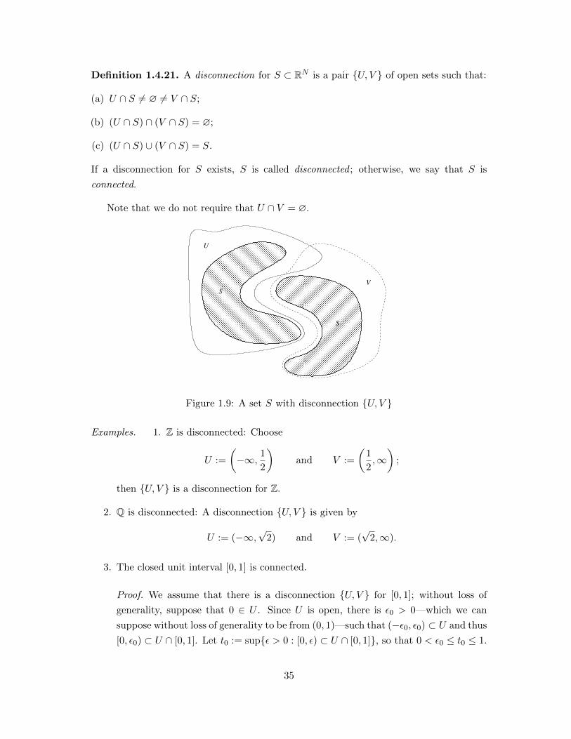
Definition 1.4.21. A disconnection for S ⊂ RN is a pair {U, V } of open sets such that:
(a) U ∩ S 6= ∅ 6= V ∩ S;
(b) (U ∩ S) ∩ (V ∩ S) = ∅;
(c) (U ∩ S) ∪ (V ∩ S) = S.
If a disconnection for S exists, S is called disconnected ; otherwise, we say that S is
connected.
Note that we do not require that U ∩ V = ∅.
����������������������������������������������������������������������������������������������������������������������������������������������������������������������������������������������������������������������������������������������������������������������������������������������������������������������������������������������������������������������������������������������������������������������������������������������������������������������������������������������������������������������������������������������������������������������������������������������������������������������������������������������������������������������������������������������������
����������������������������������������������������������������������������������������������������������������������������������������������������������������������������������������������������������������������������������������������������������������������������������������������������������������������������������������������������������������������������������������������������������������������������������������������������������������������������������������������������������������������������������������������������������������������������������������������������������������������������������������������������������������������������������������������������
��������������������������������������������������������������������������������������������������������������������������������������������������������������������������������������������������������������������������������������������������������������������������������������������������������������������������������������������������������������������������������������������������������������������������������������������������������������������������������������������������������������������������������������������������������������������������������������������
��������������������������������������������������������������������������������������������������������������������������������������������������������������������������������������������������������������������������������������������������������������������������������������������������������������������������������������������������������������������������������������������������������������������������������������������������������������������������������������������������������������������������������������������������������������������������������������������
S
S
U
V
Figure 1.9: A set S with disconnection {U, V }
Examples. 1. Z is disconnected: Choose
U :=
(−∞, 1
2
)and V :=
(1
2,∞)
;
then {U, V } is a disconnection for Z.
2. Q is disconnected: A disconnection {U, V } is given by
U := (−∞,√
2) and V := (√
2,∞).
3. The closed unit interval [0, 1] is connected.
Proof. We assume that there is a disconnection {U, V } for [0, 1]; without loss of
generality, suppose that 0 ∈ U . Since U is open, there is ε0 > 0—which we can
suppose without loss of generality to be from (0, 1)—such that (−ε0, ε0) ⊂ U and thus
[0, ε0) ⊂ U ∩ [0, 1]. Let t0 := sup{ε > 0 : [0, ε) ⊂ U ∩ [0, 1]}, so that 0 < ε0 ≤ t0 ≤ 1.
35

Assume that t0 ∈ V . We can choose δ > 0 such that t0−δ > 0 and (t0−δ, t0+δ) ⊂ V .
This, in particular, means that [0, ε) 6⊂ U ∩ [0, 1] for all ε > t0− δ, which contradicts
the very definition of t0.
Assume therefore that t0 ∈ U . If t0 < 1, we can choose θ > 0 such that t0 + θ < 1
and (t0 − θ, t0 + θ) ⊂ U : this also contradicts the definition of t0. Hence, assume
that t0 = 1. But this implies that V ∩ [0, 1] = ∅, which contradicts the definition of
a disconnection.
All in all, there is no disconnection for [0, 1].
Theorem 1.4.22. Let C ⊂ RN be convex. Then C is connected.
Proof. Assume that there is a disconnection {U, V } for C. Let x ∈ U∩C and let y ∈ V ∩C.
Let
U := {t ∈ R : tx+ (1− t)y ∈ U}
and
V := {t ∈ R : tx+ (1− t)y ∈ V }.
We claim that U is open. To see this, let t0 ∈ U . It follows that x0 := t0x+(1− t0)y ∈U . Since U is open, there is ε > 0 such that Bε(x0) ⊂ U . For t ∈ R with |t− t0| < ε
‖x‖+‖y‖ ,
we thus have
‖(tx+ (1− t)y)− x0‖ = ‖(tx+ (1− t)y)− (t0x+ (1− t0)y)‖
= ‖(t− t0)x− (t− t0)y‖
≤ |t− t0|(‖x‖+ ‖y‖)
< ε
and therefore tx+ (1− t)y ∈ Bε(x0) ⊂ U . It follows that t ∈ U .
Analogously, one sees that V is open.
The following hold for {U , V }:
(a) U ∩ [0, 1] 6= ∅ 6= V ∩ [0, 1]: since x = 1x + (1 − 1)y ∈ U and y = 0x + (1 − 0)y ∈ V ,
we have 1 ∈ U and 0 ∈ V ;
(b) (U ∩ [0, 1]) ∩ (V ∩ [0, 1]) = ∅: if t ∈ (U ∩ [0, 1]) ∩ (V ∩ [0, 1]), then tx + (1 − t)y ∈(U ∩ C) ∩ (V ∩ C), which is impossible;
(c) (U ∩ [0, 1]) ∪ (V ∩ [0, 1]) = [0, 1]: for t ∈ [0, 1], we have tx+ (1− t)y ∈ C = (U ∩C) ∪(V ∪ C)—due to the convexity of C—, so that t ∈ (U ∩ [0, 1]) ∪ (V ∩ [0, 1]).
Hence, {U , V } is a disconnection for [0, 1], which is impossible.
Example. ∅, RN , and all closed and open balls and intervals in RN are connected.
36

Corollary 1.4.23. The only subsets of RN which are both open and closed are ∅ and
RN .
Proof. Let U ⊂ RN be both open and closed, and assume that ∅ 6= U 6= RN . Then
{U,U c} would be a disconnection for RN .
Exercises
1. Let S ⊂ RN . Show that x ∈ RN is a cluster point of S if and only if each neighbor-
hood of x contains an infinite number of points in S.
2. Let S ⊂ RN be any set. Show that ∂S is closed.
3. For j = 1, . . . , N , let Ij = [aj , bj ] with aj < bj , and let I := I1×· · ·× IN . Determine
∂I. (Hint : Draw a sketch for N = 2 or N = 3.)
4. Which of the sets below are compact?
(a) {x ∈ RN : r ≤ ‖x‖ ≤ R} with 0 < r < R;
(b) {x ∈ RN : r < ‖x‖ ≤ R} with 0 < r < R;
(c){(t, sin 1
t
): t ∈ (0, 2021]
};
(d){
1n : n ∈ N
};
(e){
1n : n ∈ N
}∪ {0}.
Justify your answers.
5. Show that:
(a) if U1 ⊂ RN and U2 ⊂ RM are open, then so is U1 × U2 ⊂ RN+M ;
(b) if F1 ⊂ RN and F2 ⊂ RM are closed, then so is F1 × F2 ⊂ RN+M ;
(c) if K1 ⊂ RN and K2 ⊂ RM are compact, then so is K1 ×K2 ⊂ RN+M .
6. Show that a subset K of RN is compact if and only if it has the finite intersection
property, i.e., if {Fi : i ∈ I} is a family of closed sets in RN such that K∩⋂i∈I Fi = ∅,
then there are i1, . . . , in ∈ I such that K ∩ Fi1 ∩ · · · ∩ Fin = ∅.
7. A set S ⊂ RN is called star shaped if there is x0 ∈ S such that tx0 + (1 − t)x ∈ Sfor all x ∈ S and t ∈ [0, 1]. Show that every star shaped set is connected, and give
an example of a star shaped set that fails to be convex.
8. Let C ⊂ RN be connected. Show that C is also connected.
37

9. For ε ∈ (0, 1), determine whether or not the set{(x, y, z) ∈ R3 : 1 ≤ x2 + y2 ≤ 4, z2 ∈ [ε, 1]
}is (a) open, (b) closed, (c) compact, or (d) connected.
10. Let ∅ 6= S ⊂ RN be arbitrary, and let ∅ 6= U ⊂ RN be open. Show that
S + U := {x+ y : x ∈ S, y ∈ U}
is open.
38

Chapter 2
Limits and Continuity
2.1 Limits of Sequences
Definition 2.1.1. A sequence in a set S is a function s : N→ S.
When dealing with a sequence s : N → S, we prefer to write sn instead of s(n) and
denote the whole sequence s by (sn)∞n=1. We shall also consider, when the occasion arises,
sequences indexed over subsets of Z other than N, e.g., {n ∈ Z : n ≥ −333}.
Definition 2.1.2. A sequence (xn)∞n=1 in RN converges or is convergent to x ∈ RN if, for
each neighborhood U of x, there is nU ∈ N such that xn ∈ U for all n ≥ nU . The vector
x is called the limit of (xn)∞n=1. A sequence that does not converge is said to diverge or
to be divergent.
Equivalently, the sequence (xn)∞n=1 converges to x ∈ RN if, for each ε > 0, there is
nε ∈ N such that ‖xn − x‖ < ε for all n ≥ nε.If a sequence (xn)∞n=1 in RN converges to x ∈ RN , we write x = limn→∞ xn or xn
n→∞→ x
or simply xn → x.
Proposition 2.1.3. Every sequence in RN has at most one limit.
Proof. Let (xn)∞n=1 be a sequence in RN with limits x, y ∈ RN . Assume that x 6= y, and
set ε := ‖x−y‖2 .
Since x = limn→∞ xn, there is n1 ∈ N such that ‖xn−x‖ < ε for n ≥ n1, and since also
y = limn→∞ xn, there is n2 ∈ N such that ‖xn − y‖ < ε for n ≥ n2. For n ≥ max{n1, n2},we then have
‖x− y‖ ≤ ‖x− xn‖+ ‖xn − y‖ < 2ε = ‖x− y‖,
which is impossible.
39

n2x
n1x
y
x
Figure 2.1: Uniqueness of the limit
We call a sequence (xn)∞n=1 bounded
Proposition 2.1.4. Every convergent sequence in RN is bounded.
We omit the proof which is almost verbatim like in the one-dimensional case.
Theorem 2.1.5. Let (xn)∞n=1 =((x
(1)n , . . . , x
(N)n
))∞n=1
be a sequence in RN . Then the
following are equivalent for x =(x(1), . . . , x(N)
):
(i) limn→∞ xn = x;
(ii) limn→∞ x(j)n = x(j) for j = 1, . . . , N .
Proof. (i) =⇒ (ii): Let ε > 0. Then there is nε ∈ N such that ‖xn− x‖ < ε for all n ≥ nε,so that ∣∣∣x(j)
n − x(j)∣∣∣ ≤ ‖xn − x‖ < ε
holds for all n ≥ nε and for all j = 1, . . . , N . This proves (ii).
(ii) =⇒ (i): Let ε > 0. For each j = 1, . . . , N , there is n(j)ε ∈ N such that∣∣∣x(j)
n − x(j)∣∣∣ < ε√
N
holds for all j = 1, . . . , N and for all n ≥ n(j)ε . Let nε := max
{n
(1)ε , . . . , n
(N)ε
}. It follows
that
maxj=1,...,N
∣∣∣x(j)n − x(j)
∣∣∣ < ε√N
and thus
‖xn − x‖ ≤√N max
j=1,...,N
∣∣∣x(j)n − x(j)
∣∣∣ < ε
for all n ≥ nε.
40
Examples. 1. The sequence (1
n, 3,
3n2 − 4
n2 + 2n
)∞n=1
converges to (0, 3, 3), because 1n → 0, 3→ 3 and 3n2−4
n2+2n→ 3 in R.
2. The sequence (1
n3 + 3n, (−1)n
)∞n=1
diverges because ((−1)n)∞n=1 does not converge in R.
Since convergence in RN is nothing but coordinatewise convergence, the following is a
straightforward consequence of the limit rules in R:
Proposition 2.1.6 (Limit Rules). Let (xn)∞n=1, (yn)∞n=1 be convergent sequences in RN ,
and let (λn)∞n=1 be a convergent sequence in R. Then the sequences (xn + yn)∞n=1,
(λnxn)∞n=1, and (xn · yn)∞n=1 are also convergent such that:
limn→∞
(xn + yn) = limn→∞
xn + limn→∞
yn,
limn→∞
λnxn = ( limn→∞
λn)( limn→∞
xn)
and
limn→∞
(xn · yn) = ( limn→∞
xn) · ( limn→∞
yn).
Definition 2.1.7. Let (sn)∞n=1 be a sequence in a set S, and let n1 < n2 < · · · . Then
(snk)∞k=1 is called a subsequence of (sn)∞n=1.
As in R, we have:
Theorem 2.1.8. Every bounded sequence in RN has a convergent subsequence.
Proof. Let (xn)∞n=1 be a bounded sequence in RN , and let S := {xn : n ∈ N}.If S is finite, (xn)∞n=1 obviously has a constant and thus convergent subsequence.
Suppose therefore that S is infinite. By the Bolzano–Weierstraß Theorem, it therefore
has a cluster point x. Choose n1 ∈ N such that xn1 ∈ B1(x) \ {x}. Suppose now that
n1 < n2 < · · · < nk have already been constructed such that
xnj ∈ B 1j(x) \ {x}
for j = 1, . . . , k. Let
ε := min
{1
k + 1, ‖xl − x‖ : l = 1, . . . , nk and xl 6= x
}.
41

Then there is nk+1 ∈ N such that xnk+1∈ Bε(x) \ {x}. By the choice of ε, it is clear that
xnk+16= xl for l = 1, . . . , nk, so that that nk+1 > nk.
The subsequence (xnk)∞k=1 obtained in this fashion satisfies
‖xnk − x‖ <1
k
for all k ∈ N, so that x = limk→∞ xnk .
Definition 2.1.9. A sequence (xn)∞n=1 in R is called decreasing if x1 ≥ x2 ≥ x3 ≥ · · · and
increasing if x1 ≤ x2 ≤ x3 ≤ · · · . It is called monotone if it is increasing or decreasing.
Theorem 2.1.10. A monotone sequence converges if and only if it is bounded.
Proof. Let (xn)∞n=1 be a bounded, monotone sequence. Without loss of generality, suppose
that (xn)∞n=1 is increasing. By Theorem 2.1.8, (xn)∞n=1 has a subsequence (xnk)∞k=1 which
converges. Let x := limk→∞ xnk . We will show that actually x = limn→∞ xn.
Let ε > 0. Then there is kε ∈ N such that
x− xnk = |xnk − x| < ε,
i.e.,
x− ε < xnk < x+ ε
for all k ≥ kε. Let nε := nkε , and let n ≥ nε. Pick m ∈ N be such that nm ≥ n, and note
that xnε ≤ xn ≤ xnm , so that
x− ε < xnε ≤ xn ≤ xnm < x+ ε,
i.e.,
|x− xn| < ε.
This means that indeed x = limn→∞ xn.
Example. Let θ ∈ (0, 1), so that
0 < θn+1 = θ θn < θn ≤ 1
for all n ∈ N. Hence, the sequence (θn)∞n=1 is bounded and decreasing and thus convergent.
Since
limn→∞
θn = limn→∞
θn+1 = θ limn→∞
θn,
it follows that limn→∞ θn = 0.
Theorem 2.1.11. The following are equivalent for a set F ⊂ RN :
(i) F is closed;
42

(ii) for each sequence (xn)∞n=1 in F with limit x ∈ RN , we already have x ∈ F .
Proof. (i) =⇒ (ii): Let (xn)∞n=1 be a convergent sequence in F with limit x ∈ RN . Assume
that x /∈ F , i.e., x ∈ F c. Since F c is open, there is ε > 0 such that Bε(x) ⊂ F c. Since
x = limn→∞ xn, there is nε ∈ N such that ‖xn − x‖ < ε for all n ≥ nε. But this, in turn,
means that xn ∈ Bε(x) ⊂ F c for n ≥ nε, which is absurd.
(ii) =⇒ (i): Assume that F is not closed, i.e., F c is not open. Hence, there is x ∈ F c
such that Bε(x) ∩ F 6= ∅ for all ε > 0. In particular, there is, for each n ∈ N, an element
xn ∈ F with ‖xn − x‖ < 1n . It follows that x = limn→∞ xn even though (xn)∞n=1 lies in F
whereas x /∈ F .
Example. The set
F = {(x1, . . . , xN ) ∈ RN : x1 − x2 − · · · − xN ∈ [0, 1]}
is closed. To see this, let (xn)∞n=1 be a sequence in F which converges to some x ∈ RN .
We have
xn,1 − xn,2 − · · · − xn,N ∈ [0, 1]
for n ∈ N. Since [0, 1] is closed this means that
x1 − x2 − · · · − xN = limn→∞
(xn,1 − xn,2 − · · · − xn,N ) ∈ [0, 1],
so that x ∈ F .
Theorem 2.1.12. The following are equivalent for a set K ⊂ RN :
(i) K is compact;
(ii) every sequence in K has a subsequence that converges to a point in K.
Proof. (i) =⇒ (ii): Let (xn)∞n=1 be a sequence in K, which is then necessarily bounded.
Hence, it has a convergent subsequence with limit, say x ∈ RN . Since K is also closed, it
follows from Theorem 2.1.11 that x ∈ K.
(ii) =⇒ (i): Assume that K is not compact. By the Heine–Borel theorem, this leaves
two cases:
Case 1: K is not bounded. In this case, there is, for each n ∈ N, and element xn ∈ Kwith ‖xn‖ ≥ n. Hence, every subsequence of (xn)∞n=1 is unbounded and thus diverges.
Case 2: K is not closed. By Theorem 2.1.11, there is a sequence (xn)∞n=1 in K that
converges to a point x ∈ Kc. Since every subsequence of (xn)∞n=1 converges to x as well,
this violates (ii).
43

Corollary 2.1.13. Let ∅ 6= F ⊂ RN be closed, and let ∅ 6= K ⊂ RN be compact such
that
inf{‖x− y‖ : x ∈ K, y ∈ F} = 0.
Then F and K have non-empty intersection.
This is wrong if K is only required to be closed, but not necessarily compact:
x
y
Figure 2.2: Two closed sets in R2 with distance zero, but empty intersection
Proof. For each n ∈ N, choose xn ∈ K and yn ∈ F such that ‖xn− yn‖ < 1n . By Theorem
2.1.12, (xn)∞n=1 has a subsequence (xnk)∞k=1 converging to x ∈ K. Since limn→∞(xn−yn) =
0, it follows that
x = limk→∞
xnk = limk→∞
((xnk − ynk) + ynk) = limk→∞
ynk
and thus, from Theorem 2.1.11, x ∈ F holds as well.
Definition 2.1.14. A sequence (xn)∞n=1 in RN is called a Cauchy sequence if, for each
ε > 0, there is nε ∈ N such that ‖xn − xm‖ < ε for n,m ≥ nε.
Theorem 2.1.15. A sequence in RN is a Cauchy sequence if and only if it converges.
Proof. Let (xn)∞n=1 be a sequence in RN with limit x ∈ RN . Let ε > 0. Then there is
nε ∈ N such that ‖xn − x‖ < ε2 for all n ≥ nε. It follows that
‖xn − xm‖ ≤ ‖xn − x‖+ ‖x− xm‖ <ε
2+ε
2= ε
for n,m ≥ nε. Hence, (xn)∞n=1 is a Cauchy sequence.
Conversely, suppose that (xn)∞n=1 is a Cauchy sequence. Then there is n1 ∈ N such
that ‖xn − xm‖ < 1 for all n,m ≥ n1. For n ≥ n1, this means in particular that
‖xn‖ ≤ ‖xn − xn1‖+ ‖xn1‖ < 1 + ‖xn1‖.
44
Let
C := max{‖x1‖, . . . , ‖xn1−1‖, 1 + ‖xn1‖}.
Then it is immediate that ‖xn‖ ≤ C for all n ∈ N. Hence, (xn)∞n=1 is bounded and thus
has a convergent subsequence, say (xnk)∞k=1. Let x := limk→∞ xnk , and let ε > 0. Let
n0 ∈ N be such that ‖xn−xm‖ < ε2 for n ≥ n0, and let kε ∈ N be such that ‖xnk −x‖ < ε
2
for k ≥ kε. Let nε := nmax{kε,n0}. Then it follows that
‖xn − x‖ ≤ ‖xn − xnε‖︸ ︷︷ ︸< ε
2
+ ‖xnε − x‖︸ ︷︷ ︸< ε
2
< ε
for n ≥ nε.
Example. For n ∈ N, let
sn :=n∑k=1
1
k.
It follows that
|s2n − sn| =2n∑
k=n+1
1
k≥
2n∑k=n+1
1
2n=
1
2,
so that (sn)∞n=1 cannot be a Cauchy sequence and thus has to diverge. Since (sn)∞n=1 is
increasing, this does in fact mean that it must be unbounded.
Exercises
1. Use induction to prove Bernoulli’s Inequality, i.e.,
(1 + x)n ≥ 1 + nx
for n ∈ N0 and x ≥ −1. Conclude that, if θ > 1 and R ∈ R, there is n ∈ N such
that θn > R. Conclude that the sequence (θn)∞n=1 does not converge.
2. Let (xn)∞n=1 be a convergent sequence in RN with limit x. Show that {xn : n ∈N} ∪ {x} is compact.
3. Let (xn)∞n=1 be a sequence in RN such that there is θ ∈ (0, 1) with
‖xn+2 − xn+1‖ ≤ θ‖xn+1 − xn‖
for n ∈ N. Show that (xn)∞n=1 converges.
(Hint : Show first that
‖xn+1 − xn‖ ≤ θn−1‖x2 − x1‖
for n ∈ N, and then use this and the fact that∑∞
n=0 θn converges to show that
(xn)∞n=1 is a Cauchy sequence.)
4. Let S ⊂ RN , and let x ∈ RN . Show that x ∈ S if and only if there is a sequence
(xn)∞n=1 in S such that x = limn→∞ xn.
45

2.2 Limits of Functions
We define the limit of a function (at a point) through limits of sequences:
Definition 2.2.1. Let ∅ 6= D ⊂ RN , let f : D → RM be a function, and let x0 ∈ D.
Then L ∈ RM is called the limit of f for x → x0—in symbols: L = limx→x0 f(x)—if
limn→∞ f(xn) = L for each sequence (xn)∞n=1 in D with limn→∞ xn = x0.
It is important that x0 ∈ D: otherwise there are not sequences in D converging to x0.
For example, limx→−1√x is simply meaningless.
Examples. 1. Let D = [0,∞), and let f(x) =√x. Let (xn)∞n=1 be a sequence in D
with limn→∞ xn = x0. For n ∈ N, we have
|√xn −
√x0|2 ≤ |
√xn −
√x0|(√xn +
√x0) = |xn − x0|.
Let ε > 0, and choose nε ∈ N such that |xn − x0| < ε2 for n ≥ nε. It follows that
|√xn −
√x0| < ε
for n ≥ nε. Since ε > 0 was arbitrary, limn→∞√xn =
√x0 holds. Hence, we have
limx→x0√x =√x0.
2. LetD = (0,∞), and let f(x) = 1x . Let (xn)∞n=1 be a sequence inD with limn→∞ xn =
0. Let R > 0. Then there is n0 ∈ N such that xn0 <1R and thus f(xn0) = 1
xn0> R.
Hence, the sequence (f(xn))∞n=1 is unbounded and thus divergent. Consequently,
limx→0 f(x) does not exist.
3. Let
f : R2 \ {(0, 0)} → R, (x, y) 7→ xy
x2 + y2.
Let xn =(
1n ,
1n
), so that limn→∞ xn = 0. Then
f(xn) = f
(1
n,
1
n
)=
1n2
1n2 + 1
n2
=1
2
holds for all n ∈ N.
On the other hand, let xn =(
1n ,
1n2
), so that
f(xn) = f
(1
n,
1
n2
)=
1n3
1n2 + 1
n4
=1
n3
n4
n2 + 1=
n4
n5 + n3=
1n
1 + 1n2
→ 0.
Consequently, lim(x,y)→(0,0) f(x, y) does not exist.
As in one variable, the limit of a function at a point can be described in alternative
ways:
46

Theorem 2.2.2. Let ∅ 6= D ⊂ RN , let f : D → RM , and let x0 ∈ D. Then the following
are equivalent for L ∈ RM :
(i) limx→x0 f(x) = L;
(ii) for each ε > 0, there is δ > 0 such that ‖f(x) − L‖ < ε for each x ∈ D with
‖x− x0‖ < δ;
(iii) for each neighborhood U of L, there is a neighborhood V of x0 such that f−1(U) =
V ∩D.
Proof. (i) =⇒ (ii): Assume that (i) holds, but that (ii) is false. Then there is ε0 > 0
sucht that, for each δ > 0, there is xδ ∈ D with ‖xδ − x0‖ < δ, but ‖f(xδ)− L‖ ≥ ε0. In
particular, for each n ∈ N, there is xn ∈ D with ‖xn − x0‖ < 1n , but ‖f(xn)− L‖ ≥ ε0. It
follows that limn→∞ xn = x0 whereas f(xn) 6→ L. This contradicts (i).
(ii) =⇒ (iii): Let U be a neighborhood of L. Choose ε > 0 such that Bε(L) ⊂ U , and
choose δ > 0 as in (ii). It follows that
D ∩Bδ(x0) ⊂ f−1(Bε(L)) ⊂ f−1(U).
Let V := Bδ(x0) ∪ f−1(U).
(iii) =⇒ (i): Let (xn)∞n=1 be a sequence in D with limn→∞ xn = x0. Let U be a
neighborhood of L. By (iii), there is a neighborhood V of x0 such that f−1(U) = V ∩D.
Since x0 = limn→∞ xn, there is nV ∈ N such that xn ∈ V for all n ≥ nV . Conse-
quently, f(xn) ∈ U for all n ≥ nV . Since U is an arbitrary neighborhood of L, we have
limn→∞ f(xn) = L. Since (xn)∞n=1 is an arbitrary sequence in D converging to x0, (i)
follows.
Definition 2.2.3. Let ∅ 6= D ⊂ RN , let f : D → RM , and let x0 ∈ D. Then f is
continuous at x0 if limx→x0 f(x) = f(x0).
Applying Theorem 2.2.2 with L = f(x0) yields:
Theorem 2.2.4. Let ∅ 6= D ⊂ RN , let f : D → RM , and let x0 ∈ D. Then the following
are equivalent:
(i) f is continuous at x0;
(ii) for each ε > 0, there is δ > 0 such that ‖f(x) − f(x0)‖ < ε for each x ∈ D with
‖x− x0‖ < δ;
(iii) for each neighborhood U of f(x0), there is a neighborhood V of x0 such that f−1(U) =
V ∩D.
47

Continuity in several variables has hereditary properties similar to those in the one
variable situation:
Proposition 2.2.5. Let ∅ 6= D ⊂ RN , and let f, g : D → RM and φ : D → R be
continuous at x0 ∈ D. Then the functions
f + g : D → RM , x 7→ f(x) + g(x),
φf : D → RM , x 7→ φ(x)f(x),
and
f · g : D → RM , x 7→ f(x) · g(x)
are continuous at x0.
Proposition 2.2.6. Let ∅ 6= D1 ⊂ RN , ∅ 6= D2 ⊂ RM , let f : D2 → RK and g : D1 →RM be such that g(D1) ⊂ D2, and let x0 ∈ D1 be such that g is continuous at x0 and that
f is continuous at g(x0). Then
f ◦ g : D1 → RK , x 7→ f(g(x))
is continuous at x0.
Proof. Let (xn)∞n=1 be a sequence in D such that xn → x0. Since g is continuous at
x0, we have g(xn) → g(x0), and since f is continuous at g(x0), this ultimately yields
f(g(xn))→ f(g(x0)).
Proposition 2.2.7. Let ∅ 6= D ⊂ RN . Then f = (f1, . . . , fM ) : D → RM is continuous
at x0 ∈ D if and only if fj : D → R is continuous at x0 for j = 1, . . . ,M .
Examples. 1. The function
f : R2 → R3, (x, y) 7→(
sin
(xy2
x2 + y4 + π
), e
y17
sin(log(π+cos(x)2)) , 2021
)is continuous at every point of R2.
2. Let
f : R→ R2, x 7→
{(x, 1), x ≤ 0,
(x,−1), x > 0,
so that
f1 : R→ R, x 7→ x
and
f2 : R→ R, x 7→
{1, x ≤ 0,
−1, x > 0.
It follows that f1 is continuous at every point of R, where is f2 is continuous only
at x0 6= 0. It follows that f is continuous at every point x0 6= 0, but discontinuous
at x0 = 0.
48

Exercises
1. Let D := {(x, y) ∈ R2 : y 6= 0}, and let
f : D → R, (x, y) 7→ x2
y
Show that:
(a) limt→0t6=0
f(tx0, ty0) = 0 for all (x0, y0) ∈ D;
(b) lim(x,y)→(0,0) f(x, y) does not exist.
2. Let
f : R3 \ {0} → R, (x, y, z) 7→ xyz
|x|3 + |y|3 + |z|3.
Calculate
limn→∞
f
(1
n,
1
n,
1
n
)and lim
n→∞f
(1
n,
1
n,
1
n2
).
What does this tell you about lim(x,y,z)→(0,0,0) f(x, y, z)?
2.3 Global Properties of Continuous Functions
So far, we have discussed continuity only in local terms, i.e., at a point. In this section,
we shall consider continuity globally.
Definition 2.3.1. Let ∅ 6= D ⊂ RN . A function f : D → RM is continuous on D if it is
continuous at each point x0 ∈ D.
Theorem 2.3.2. Let ∅ 6= D ⊂ RN . Then the following are equivalent for f : D → RM :
(i) f is continuous.
(ii) for each open U ⊂ RM , there is an open set V ⊂ RN such that f−1(U) = V ∩D.
Proof. (i) =⇒ (ii): Let U ⊂ RM be open, and let x ∈ D such that f(x) ∈ U , i.e.,
x ∈ f−1(U). Since U is open, there is εx > 0 such that Bεx(f(x)) ⊂ U . Since f
is continuous at x, there is δx > 0 such that ‖f(y) − f(x)‖ < εx for all y ∈ D with
‖y − x‖ < δx, i.e.,
Bδx(x) ∩D ⊂ f−1(Bεx(f(x))) ⊂ f−1(U).
Letting V :=⋃x∈f−1(U)Bδx(x), we obtain an open set such that
f−1(U) ⊂ V ∩D ⊂ f−1(U).
(ii) =⇒ (i): Let x0 ∈ D, and choose ε > 0. Then there is an open subset V of RN
such that V ∩D = f−1(Bε(f(x0))). Choose δ > 0 such that Bδ(x0) ⊂ V . It follows that
‖f(x)− f(x0)‖ < ε for all x ∈ D with ‖x− x0‖ < δ. Hence, f is continuous at x0.
49
Corollary 2.3.3. Let ∅ 6= D ⊂ RN . Then the following are equivalent for f : D → RM :
(i) f is continuous.
(ii) for each closed F ⊂ RM , there is a closed set G ⊂ RN such that f−1(F ) = G ∩D.
Proof. (i) =⇒ (ii): Let F ⊂ RM be closed. By Theorem 2.3.2, there is an open set V ⊂ RN
such that
V ∩D = f−1(F c) = f−1(F )c.
Let G := V c.
(ii) =⇒ (i): Let U ⊂ RM be open. By (ii), there is a closed set G ⊂ RN with
G ∩D = f−1(U c) = f−1(U)c.
Letting V := Gc, we obtain an open set with V ∩D = f−1(U). By Theorem 2.3.2, this
implies the continuity of f .
Example. The set
F = {(x, y, z, u) ∈ R4 : ex+y sin(zu2) ∈ [0, 2] and x− y2 + z3 − u4 ∈ [−π, 2020]}
is closed. This can be seen as follows: The function
f : R4 → R2, (x, y, z, u) 7→ (ex+y sin(zu2), x− y2 + z3 − u4)
is continuous, [0, 2]× [−π, 2020] is closed, and F = f−1([0, 2]× [−π, 2020]).
Theorem 2.3.4. Let ∅ 6= K ⊂ RN be compact, and let f : K → RM be continuous. Then
f(K) is compact.
Proof. Let {Ui : i ∈ I} be an open cover for f(K). By Theorem 2.3.2, there is, for each
i ∈ I an open subset Vi of RN such that Vi ∩K = f−1(Ui). Then {Vi : i ∈ I} is an open
cover for K. Since K is compact, there are i1, . . . , in ∈ I such that
K ⊂ Vi1 ∪ · · · ∪ Vin .
Let x ∈ K. Then there is j ∈ {1, . . . , n} such that x ∈ Vij and thus f(x) ∈ Uij . It follows
that
f(K) ⊂ Ui1 ∪ · · · ∪ Uin ,
so that f(K) is compact.
Corollary 2.3.5. Let ∅ 6= K ⊂ RN be compact, and let f : K → RM be continuous.
Then f(K) is bounded.
50

Corollary 2.3.6. Let ∅ 6= K ⊂ RN be compact, and let f : K → R be continuous. Then
there are xmax, xmin ∈ K such that
f(xmax) = sup{f(x) : x ∈ K} and f(xmin) = inf{f(x) : x ∈ K}.
Proof. Let (yn)∞n=1 be a sequence in f(K) such that yn → y0 := sup{f(x) : x ∈ K}. Since
f(K) is compact and thus closed, there is xmax ∈ K such that f(xmax) = y0
The existence of xmin is shown similarly.
The two previous corollaries generalize two well known results on continuous functions
on closed, bounded intervals of R. They show that the crucial property of an interval, say
[a, b] that makes these results work in one variable is precisely compactness.
The intermediate value theorem does not extend to continuous functions on arbitrary
compact set, as can be seen by very easy examples. The crucial property of [a, b] that
makes this particular theorem work is not compactness, but connectedness.
Theorem 2.3.7. Let ∅ 6= D ⊂ RN be connected, and let f : D → RM be continuous.
Then f(D) is connected.
Proof. Assume that there is a disconnection {U, V } for f(D). Since f is continuous, there
are open sets U , V ⊂ RN open such that
U ∩D = f−1(U) and V ∩D = f−1(V ).
But then {U , V } is a disconnection for D, which is impossible.
This theorem can be used, for example, to show that certain sets are connected:
Example. The unit circle in the plane
S1 := {(x, y) ∈ R2 : ‖(x, y)‖ = 1}
is connected because R is connected,
f : R→ R2, t 7→ (cos t, sin t)
is continuous, and S1 = f(R). (Inductively, one can then go on and show that SN−1 is
connected for all N ≥ 2.)
Corollary 2.3.8 (Intermediate Value Theorem). Let ∅ 6= D ⊂ RN be connected, let
f : D → R be continuous, and let x1, x2 ∈ D be such that f(x1) < f(x2). Then, for each
y ∈ (f(x1), f(x2)), there is xy ∈ D with f(xy) = y.
Proof. Assume that there is y0 ∈ (f(x1), f(x2)) with y0 /∈ f(D). Then {U, V } with
U := {y ∈ R : y < y0} and V := {y ∈ R : y > y0}
is a disconnection for f(D), which contradicts Theorem 2.3.7.
51

Examples. 1. Let p be a polynomial of odd degree with leading coefficient one, so that
limx→∞
p(x) =∞ and limx→−∞
p(x) = −∞.
Hence, there are x1, x2 ∈ R such that p(x1) < 0 < p(x2). By the Intermediate Value
Theorem, there is x ∈ R with p(x) = 0.
2. Let
D := {(x, y, z) ∈ R3 : ‖(x, y, z)‖ ≤ π},
so that D is connected. Let
f : D → R, (x, y, z) 7→ xy + z
cos(xyz)2 + 1.
Then
f(0, 0, 0) = 0 and f(1, 0, 1) =1
1 + 1=
1
2.
Hence, there is (x0, y0, z0) ∈ D such that f(x0, y0, z0) = 1π .
Exercises
1. Let K,L ⊂ RN compact and non-empty. Show that
K + L := {x+ y : x ∈ K, y ∈ L}
is compact in RN .
2. Let C ⊂ RN . We say that x0, x1 ∈ C can be joined by a path if there is a continuous
function γ : [0, 1] → RN with γ([0, 1]) ⊂ C, γ(0) = x0, and γ(1) = x1. We call C
path connected if any two points in C can be joined by a path.
Show that any path connected set is connected.
3. Show that:
(a) if C1 ⊂ RN1 and C2 ⊂ RN2 are path connected, then so is C1 × C2 ⊂ RN1+N2 ;
(b) if C ⊂ RN is path connected and f : C → RM is continuous, then f(C) is path
connected;
(c) if C1, C2 ⊂ RN is path connected, then so is C1 + C2.
4. Show that:
(a) if C is a family of connected subsets of RN such that⋂C∈C C 6= ∅, then
⋃C∈C C
is connected;
52

(b) if C1 ⊂ RN1 and C2 ⊂ RN2 are connected, then so is C1×C2 ⊂ RN1+N2 (Hint :
Argue that we can suppose that C1 and C2 are not empty, and fix x2 ∈ C2;
then apply (a) to C := {(C1 × {x2}) ∪ ({x1} × C2) : x1 ∈ C1}.);
(c) if C1, C2 ⊂ RN are connected, then so is C1 + C2 ⊂ RN .
5. Let
C :=
{(x, sin
(1
x
)): x > 0
}⊂ R2.
Show that C is connected, but not path connected. (Hint : Show that {0}×[−1, 1] ⊂C and that any point in {0} × [−1, 1] cannot be joined by a path with any point of
the form(x, sin
(1x
))with x > 0.)
6. Show that RN \ {0} is disconnected if and only if N = 1.
7. Let
D := {(exy, e−x2−z) : (x, y, z) ∈ R3}
Short that there is (u, v) ∈ D such that
log(u+ v) =√
19.
2.4 Uniform Continuity
We conclude the chapter on continuity, with a property related to, but stronger than
continuity:
Definition 2.4.1. Let ∅ 6= D ⊂ RN . Then f : D → RM is called uniformly continuous
if, for each ε > 0, there is δ > 0 such that ‖f(x1) − f(x2)‖ < ε for all x1, x2 ∈ D with
‖x1 − x2‖ < δ.
The difference between uniform continuity and continuity at every point is that the
δ > 0 in the definition of uniform continuity depends only on ε > 0, but not on a particular
point of the domain.
Examples. 1. All constant functions are uniformly continuous.
2. The function
f : [0, 1]→ R, x 7→ x2
is uniformly continuous. To see this, let ε > 0, and observe that
|x21 − x2
2| = |x1 − x2|(x1 + x2) ≤ 2|x1 − x2|
for all x1, x2 ∈ [0, 1]. Choose δ := ε2 .
53

3. The function
f : (0, 1]→ R, x 7→ 1
x
is continuous, but not uniformly continuous. For each n ∈ N, we have∣∣∣∣f ( 1
n
)− f
(1
n+ 1
)∣∣∣∣ = |n− (n+ 1)| = 1.
Therefore, there is no δ > 0 such that∣∣∣f ( 1
n
)− f
(1
n+1
)∣∣∣ < 12 whenever
∣∣∣ 1n −
1n+1
∣∣∣ <δ.
4. The function
f : [0,∞)→ R, x 7→ x2
is continuous, but not uniformly continuous. Assume that there is δ > 0 such that
|f(x1) − f(x2)| < 1 for all x1, x2 ≥ 0 with |x1 − x2| < δ. Choose, x1 := 2δ and
x2 := 2δ + δ
2 . It follows that |x1 − x2| = δ2 < δ. However, we have
|f(x1)− f(x2)| = |x1 − x2|(x1 + x2)
=δ
2
(2
δ+
2
δ+δ
2
)≥ δ
2
4
δ
= 2.
The following theorem is very valuable when it comes to determining that a given
function is uniformly continuos:
Theorem 2.4.2. Let ∅ 6= K ⊂ RN be compact, and let f : K → RM be continuous. Then
f is uniformly continuous.
Proof. Assume that f is not uniformly continuous, i.e., there is ε0 > 0 such that, for all
δ > 0, there are xδ, yδ ∈ K with ‖xδ−yδ‖ < δ whereas ‖f(xδ)−f(yδ)‖ ≥ ε0. In particular,
there are, for each n ∈ N, elements xn, yn ∈ K such that
‖xn − yn‖ <1
nand ‖f(xn)− f(yn)‖ ≥ ε0.
Since K is compact, (xn)∞n=1 has a subsequence (xnk)∞k=1 converging to some x ∈ K. Since
xnk − ynk → 0, it follows that
x = limk→∞
xnk = limk→∞
ynk .
The continuity of f yields
f(x) = limk→∞
f(xnk) = limk→∞
f(ynk).
54

Hence, there are k1, k2 ∈ N such that
‖f(x)− f(xnk)‖ < ε02
for k ≥ k1 and ‖f(x)− f(ynk)‖ < ε02
for k ≥ k2.
For k ≥ max{k1, k2}, we thus have
‖f(xnk)− f(ynk)‖ ≤ ‖f(xnk)− f(x)‖+ ‖f(x)− f(ynk)‖ < ε02
+ε02
= ε0,
which is a contradiction.
Exercises
1. Let ∅ 6= D ⊂ RN . A function f : D → RM is called Lipschitz continuous if there is
C ≥ 0 such that
‖f(x)− f(y)‖ ≤ C‖x− y‖
for all x, y ∈ D.
Show that:
(a) each Lipschitz continuous function is uniformly continuous;
(b) if f : [a, b] → R is continuous such that f is differentiable on (a, b) with f ′
bounded on (a, b), then f is Lipschitz continuous;
(c) the function
f : [0, 1]→ R, x 7→√x
is uniformly continuous, but not Lipschitz continuous.
2. (Banach’s Fixed Point Theorem.) Let ∅ 6= F ⊂ RN be closed, and let f : F → RN
be such that f(F ) ⊂ F and that there is θ ∈ (0, 1) with
‖f(x)− f(y)‖ ≤ θ‖x− y‖
for x, y ∈ F . Show that there is a unique x0 ∈ F such that f(x0) = x0. (Hint :
Problem 2.1.3.)
3. Let ∅ 6= D ⊂ RN , let f : D → RM be continuous, and let (xn)∞n=1 be a Cauchy
sequence in D. Show that (f(xn))∞n=1 is a Cauchy sequence in RM if D is closed or
if f is uniformly continuous.
Does this remain true without any additional requirements for D or f?
55

Chapter 3
Differentiation in RN
3.1 Differentiation in One Variable: A Review
In this section, we give a quick review of differentiation in one variable.
Definition 3.1.1. Let I ⊂ R be an interval, and let x0 ∈ I. Then f : I → R is said to be
differentiable at x0 if
limh→0h6=0
f(x0 + h)− f(x0)
h
exists. This limit is denoted by f ′(x0) and called the first derivative of f at x0.
Intuitively, differentiability of f at x0 means that we can put a tangent line to the
curve given by f at (x0, f(x0)) of which the slope is f ′(x0):
f(x)
x 0 x 1
y
x
Figure 3.1: Tangent lines to f(x) at x0 and x1
Example. Let n ∈ N, and let
f : R→ R, x 7→ xn.
56
Let h ∈ R \ {0}. From the Binomial Theorem, we know that
(x+ h)n =
n∑j=0
(n
j
)xjhn−j
and thus
(x+ h)n − xn =n−1∑j=0
(n
j
)xjhn−j .
Letting h→ 0, we obtain
(x+ h)n − xn
h=
n−1∑j=0
(n
j
)xjhn−j−1
=
n−2∑j=0
(n
j
)xjh
>0︷ ︸︸ ︷n− j − 1 + nxn−1
→ nxn−1.
Proposition 3.1.2. Let I ⊂ R be an interval, and let f : I → R be differentiable at
x0 ∈ I. Then f is continuous at x0.
Proof. Let (xn)∞n=1 be a sequence in I such that xn → x0. Without loss of generality,
suppose that xn 6= x0 for all n ∈ N. It follows that
|f(xn)− f(x0)| = |xn − x|︸ ︷︷ ︸→0
∣∣∣∣f(xn)− f(x0)
xn − x0
∣∣∣∣︸ ︷︷ ︸→|f ′(x0)|
→ 0.
Hence, f is continuous at x0.
We recall the differentiation rules without proof:
Proposition 3.1.3 (Rules of Differentiation). Let I ⊂ R be an interval, and let f, g : I →R be differentiable at x0 ∈ I. Then f + g, fg, and—if g(x0) 6= 0, f
g—are differentiable at
x0 such that
(f + g)′(x0) = f ′(x0) + g′(x0),
(fg)′(x0) = f(x0)g′(x0) + f ′(x0)g(x0),
and (f
g
)′(x0) =
f ′(x0)g(x0)− f(x0)g′(x0)
g(x0)2.
57

Proposition 3.1.4 (Chain Rule). Let I, J ⊂ R be intervals, let g : I → R and f : J → Rbe functions such that g(I) ⊂ J , and suppose that g is differentiable at x0 ∈ I and that f
is differentiable at g(x0) ∈ J . Then f ◦ g : I → R is differentiable at x0 such that
(f ◦ g)′(x0) = f ′(g(x0))g′(x0).
Definition 3.1.5. Let I ⊂ R be an interval. We call f : I → R differentiable if it is
differentiable at each point of I.
Example. Define
f : R→ R, x 7→
{x2 sin
(1x
), x 6= 0,
0, x = 0.
It is clear f is differentiable at all x 6= 0 with
f ′(x) = 2x sin
(1
x
)− x2 1
x2cos
(1
x
)= 2x sin
(1
x
)− cos
(1
x
).
Let h 6= 0. Then we have∣∣∣∣f(0 + h)− f(0)
h
∣∣∣∣ =
∣∣∣∣1hh2 sin
(1
h
)∣∣∣∣ =
∣∣∣∣h sin
(1
h
)∣∣∣∣ ≤ |h| h→0→ 0,
so that f is also differentiable at x = 0 with f ′(0) = 0. Let xn := 12πn , so that xn → 0. It
follows that
f ′(xn) =1
πnsin(2πn)︸ ︷︷ ︸
=0
− cos(2πn)︸ ︷︷ ︸=1
6→ f ′(0).
Hence, f ′ is not continuous at x = 0.
Definition 3.1.6. Let ∅ 6= D ⊂ R, and let x0 be an interior point ofD. Then f : D → R is
said to have a local maximum [minimum] at x0 if there is ε > 0 such that (x0−ε, x0+ε) ⊂ Dand f(x) ≤ f(x0) [f(x) ≥ f(x0)] for all x ∈ (x0 − ε, x0 + ε). If f has a local maximum or
minimum at x0, we say that f has a local extremum at x0.
Theorem 3.1.7. Let ∅ 6= D ⊂ R, let f : D → R have a local extremum at x0 ∈ int D,
and suppose that f is differentiable at x0. Then f ′(x0) = 0 holds.
Proof. We only treat the case of a local maximum.
Let ε > 0 be as in Definition 3.1.6. For h ∈ (−ε, 0), we have x0 + h ∈ (x0 − ε, x0 + ε),
so that≤0︷ ︸︸ ︷
f(x0 + h)− f(x0)
h︸︷︷︸≤0
≥ 0.
58

It follows that f ′(x0) ≥ 0. On the other hand, we have for h ∈ (0, ε) that
≤0︷ ︸︸ ︷f(x0 + h)− f(x0)
h︸︷︷︸≥0
≤ 0,
so that f ′(x0) ≤ 0.
Consequently, f ′(x0) = 0 holds.
Lemma 3.1.8 (Rolle’s “Theorem”). Let a < b, and let f : [a, b] → R be continuous such
that f(a) = f(b) and such that f is differentiable on (a, b). Then there is ξ ∈ (a, b) such
that f ′(ξ) = 0.
Proof. The claim is clear if f is constant. Hence, we may suppose that f is not constant.
Since f is continuous, there is ξ1, ξ2 ∈ [a, b] such that
f(ξ1) = sup{f(x) : x ∈ [a, b]} and f(ξ2) = inf{f(x) : x ∈ [a, b]}.
Since f is not constant and since f(a) = f(b), it follows that f attains at least one local
extremum at some point ξ ∈ (a, b). By Theorem 3.1.7, this means f ′(ξ) = 0.
Theorem 3.1.9 (Mean Value Theorem). Let a < b, and let f : [a, b] → R be continuous
and differentiable on (a, b). Then there is ξ ∈ (a, b) such that
f ′(ξ) =f(b)− f(a)
b− a.
(f x )
y
xa bξ
Figure 3.2: Mean Value Theorem
59
Proof. Define g : [a, b]→ R by letting
g(x) := (f(x)− f(a))(b− a)− (f(b)− f(a))(x− a)
for x ∈ [a, b]. It follows that g(a) = g(b) = 0. By Rolle’s theorem, there is ξ ∈ (a, b) such
that
0 = g′(ξ) = f ′(ξ)(b− a)− (f(b)− f(a)),
which yields the claim.
Corollary 3.1.10. Let I ⊂ R be an interval, and let f : I → R be differentiable such that
f ′ ≡ 0. Then f is constant.
Proof. Assume that f is not constant. Then there are a, b ∈ I, a < b such that f(a) 6= f(b).
By the mean value theorem, there is ξ ∈ (a, b) such that
0 = f ′(ξ) =f(b)− f(a)
b− a6= 0,
which is a contradiction.
3.2 Partial Derivatives
The notion of partial differentiability is the weakest of the several generalizations of dif-
ferentiablity to several variables.
Definition 3.2.1. Let ∅ 6= D ⊂ RN , and let x0 ∈ int D. Then f : D → RM is called
partially differentiable at x0 if, for each j = 1, . . . , N , the limit
limh→0h6=0
f(x0 + hej)− f(x0)
h
exists, where ej is the j-th canonical basis vector of RN .
We use the notations
∂f∂xj
(x0)
Djf(x0)
fxj (x0)
:= limh→0h6=0
f(x0 + hej)− f(x0)
h
for the (first) partial derivative of f at x0 with respect to xj .
To calculate ∂f∂xj
, fix x1, . . . , xj−1, xj+1, . . . , xN , i.e., treat them as constants, and con-
sider f as a function of xj .
60

Examples. 1. Let
f : R2 → R, (x, y) 7→ ex + x cos(xy).
It follows that
∂f
∂x(x, y) = ex + cos(xy)− xy sin(xy) and
∂f
∂y(x, y) = −x2 sin(xy).
2. Let
f : R3 → R, (x, y, z) 7→ exp(x sin(y)z2).
We obtain
∂f
∂x(x, y, z) = sin(y)z2 exp(x sin(y)z2),
∂f
∂y(x, y, z) = x cos(y)z2 exp(x sin(y)z2),
and∂f
∂z(x, y, z) = 2zx sin(y) exp(x sin(y)z2).
3. Let
f : R2 → R, (x, y) 7→
{xy
x2+y2, (x, y) 6= (0, 0),
0, (x, y) = (0, 0).
Since
f
(1
n,
1
n
)=
1n2
1n2 + 1
n2
=1
26→ 0,
the function f is not continuous at (0, 0). Clearly, f is partially differentiable at
each (x, y) 6= (0, 0) with
∂f
∂x(x, y) =
y(x2 + y2)− 2x2y
(x2 + y2)2.
Moreover, we have∂f
∂x(0, 0) = lim
h→0h6=0
f(h, 0)− f(0, 0)
h= 0.
Hence, ∂f∂x exists everywhere.
The same is true for ∂f∂y .
Definition 3.2.2. Let ∅ 6= D ⊂ RN , let x0 ∈ int D, and let f : D → R be partially
differentiable at x0. Then the gradient (vector) of f at x0 is defined as
(grad f)(x0) := (∇f)(x0) :=
(∂f
∂x1(x0), . . . ,
∂f
∂xN(x0)
).
61
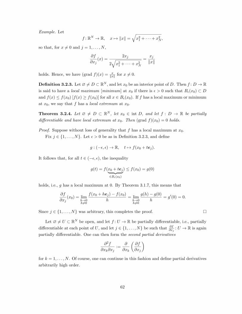
Example. Let
f : RN → R, x 7→ ‖x‖ =√x2
1 + · · ·+ x2N ,
so that, for x 6= 0 and j = 1, . . . , N ,
∂f
∂xj(x) =
2xj
2√x2
1 + · · ·+ x2N
=xj‖x‖
holds. Hence, we have (grad f)(x) = x‖x‖ for x 6= 0.
Definition 3.2.3. Let ∅ 6= D ⊂ RN , and let x0 be an interior point of D. Then f : D → Ris said to have a local maximum [minimum] at x0 if there is ε > 0 such that Bε(x0) ⊂ D
and f(x) ≤ f(x0) [f(x) ≥ f(x0)] for all x ∈ Bε(x0). If f has a local maximum or minimum
at x0, we say that f has a local extremum at x0.
Theorem 3.2.4. Let ∅ 6= D ⊂ RN , let x0 ∈ int D, and let f : D → R be partially
differentiable and have local extremum at x0. Then (grad f)(x0) = 0 holds.
Proof. Suppose without loss of generality that f has a local maximum at x0.
Fix j ∈ {1, . . . , N}. Let ε > 0 be as in Definition 3.2.3, and define
g : (−ε, ε)→ R, t 7→ f(x0 + tej).
It follows that, for all t ∈ (−ε, ε), the inequality
g(t) = f(x0 + tej︸ ︷︷ ︸∈Bε(x0)
) ≤ f(x0) = g(0)
holds, i.e., g has a local maximum at 0. By Theorem 3.1.7, this means that
∂f
∂xj(x0) = lim
h→0h6=0
f(x0 + hej)− f(x0)
h= lim
h→0h6=0
g(h)− g(0)
h= g′(0) = 0.
Since j ∈ {1, . . . , N} was arbitrary, this completes the proof.
Let ∅ 6= U ⊂ RN be open, and let f : U → R be partially differentiable, i.e., partially
differentiable at each point of U , and let j ∈ {1, . . . , N} be such that ∂f∂xj
: U → R is again
partially differentiable. One can then form the second partial derivatives
∂2f
∂xk∂xj:=
∂
∂xk
(∂f
∂xj
)for k = 1, . . . , N . Of course, one can continue in this fashion and define partial derivatives
arbitrarily high order.
62

Example. Let U := {(x, y) ∈ R2 : x 6= 0}, and define
f : U → R, (x, y) 7→ exy
x.
It follows that
∂f
∂x=xyexy − exy
x2
=xy − 1
x2exy
=
(y
x− 1
x2
)exy,
and
∂f
∂y= exy.
For the second partial derivatives, this means that
∂2f
∂x2=
(− y
x2+
2
x3
)exy +
(y
x− 1
x2
)yexy,
∂2f
∂y2= xexy,
∂2f
∂x∂y= yexy,
and
∂2f
∂y∂x=
1
xexy +
(y
x− 1
x2
)xexy =
1
xexy +
(y − 1
x
)exy = yexy.
This means that∂2f
∂x∂y=
∂2f
∂y∂x.
holds. Is this coincidence?
Theorem 3.2.5 (Clairaut’s Theorem). Let ∅ 6= U ⊂ RN be open, and suppose that
f : U → R is twice continuously partially differentiable, i.e., all second partial derivatives
of f exist and are continuous on U . Then
∂2f
∂xj∂xk(x) =
∂2f
∂xk∂xj(x)
holds for all x ∈ U and for all j, k = 1, . . . , N .
Proof. Without loss of generality, let N = 2 and x = 0.
63

Since U is open, there is ε > 0 such that (−ε, ε)2 ⊂ U . Fix y ∈ (−ε, ε), and define
Fy : (−ε, ε)→ R, x 7→ f(x, y)− f(x, 0).
Then Fy is differentiable. By the Mean Value Theorem, there is, for each x ∈ (−ε, ε), an
element ξ ∈ (−ε, ε) with |ξ| ≤ |x| such that
Fy(x)− Fy(0) = F ′y(ξ)x =
(∂f
∂x(ξ, y)− ∂f
∂x(ξ, 0)
)x.
Applying the Mean Value Theorem to the function
(−ε, ε)→ R, y 7→ ∂f
∂x(ξ, y),
we obtain η with |η| ≤ |y| such that
∂f
∂x(ξ, y)− ∂f
∂x(ξ, 0) =
∂2f
∂y∂x(ξ, η)y.
Consequently,
f(x, y)− f(x, 0)− f(0, y) + f(0, 0) = Fy(x)− Fy(0) =∂2f
∂y∂x(ξ, η)xy
holds.
Now, fix x ∈ (−ε, ε), and define
Fx : (−ε, ε)→ R, y 7→ f(x, y)− f(0, y).
Proceeding as with Fy, we obtain ξ, η with |ξ| ≤ |x| and |η| ≤ |y| such that
f(x, y)− f(0, y)− f(x, 0) + f(0, 0) =∂2f
∂x∂y(ξ, η)xy.
Therefore,∂2f
∂y∂x(ξ, η) =
∂2f
∂x∂y(ξ, η)
holds whenever xy 6= 0. Let 0 6= x → 0 and 0 6= y → 0. It follows that ξ → 0, ξ → 0,
η → 0, and η → 0. Since ∂2f∂y∂x and ∂2f
∂x∂y are continuous, this yields
∂2f
∂y∂x(0, 0) =
∂2f
∂x∂y(0, 0)
as claimed.
The usefulness of Clairaut’s Theorem appears to be limited: in order to be able to
interchange the order of differentiation, we first need to know that the second oder partial
derivatives are continuous, i.e., we need to know the second oder partial derivatives before
the theorem can help us save any work computing them. For many functions, however,
e.g., for
f : R3 → R, (x, y, z) 7→ arctan(x2 − y7)
exyz,
it is immediate from the rules of differentiation that their higher order partial derivatives
are continuous again without explicitly computing them.
64
Exercises
1. Show that the mean value theorem becomes false for vector valued functions: Let
f : [0, 2π]→ R2, x 7→ (cos(x), sin(x)).
Show that there is no ξ ∈ (0, 2π) such that
f ′(ξ) =f(2π)− f(0)
2π.
2. Let
f : R2 → R, (x, y) 7→
{xy x
2−y2x2+y2
, if (x, y) 6= (0, 0),
0, otherwise.
Show that f is twice partially differentiable everywhere, but that
∂2f
∂y∂x(0, 0) 6= ∂2f
∂x∂y(0, 0).
Is f continuous at (0, 0)?
3. Calculate all partial derivatives up to order two of the functions
f(x, y) := x2 − 42xy3 − yx and f(x, y, z) :=xey
z
where z 6= 0 for the latter function.
3.3 Vector Fields
Suppose that there is a force field in some region of space. Mathematically, a force is a
vector in R3. Hence, one can mathematically describe a force field as a function v that
that assigns to each point x in a region, say D, of R3 a force v(x).
Slightly generalizing this, we thus define:
Definition 3.3.1. Let ∅ 6= D ⊂ RN . A vector field on D is a function v : D → RN .
Example. Let ∅ 6= U ⊂ RN be open, and let f : U → R be partially differentiable. Then
∇f is a vector field on U , a so-called gradient field.
Is every vector field a gradient field?
Definition 3.3.2. Let ∅ 6= U ⊂ R3 be open, and let v : U → R3 be partially differentiable.
Then the curl of v is defined as
curl v :=
(∂v3
∂x2− ∂v2
∂x3,∂v1
∂x3− ∂v3
∂x1,∂v2
∂x1− ∂v1
∂x2
).
65

Very loosely speaking, one can say that the curl of a vector field measures “the tendency
of the field to swirl around”.
Proposition 3.3.3. Let ∅ 6= U ⊂ R3 be open, and let f : U → R be twice continuously
differentiable. Then curl grad f = 0 holds.
Proof. We have, by Theorem 3.2.5, that
curl grad f =
(∂
∂x2
∂f
∂x3− ∂
∂x3
∂f
∂x2,∂
∂x3
∂f
∂x1− ∂
∂x1
∂f
∂x3,∂
∂x1
∂f
∂x2− ∂
∂x2
∂f
∂x1
)= 0
holds.
Definition 3.3.4. Let ∅ 6= U ⊂ RN be open, and let v : U → RN be a partially
differentiable vector field. Then the divergence of v is defined as
div v :=N∑j=1
∂vj∂xj
.
Examples. 1. Let ∅ 6= U ⊂ RN be open, and let v : U → RN and f : U → R be
partially differentiable. Since
∂
∂xj(fvj) =
∂f
∂xjvj + f
∂vj∂xj
for j = 1, . . . , N , it follows that
div fv =N∑j=1
∂
∂xj(fvj)
=N∑j=1
∂f
∂xjvj + f
N∑j=1
∂vj∂xj
= ∇f · v + f div v.
2. Let
v : RN \ {0} → RN , x 7→ x
‖x‖.
Then v = fu with
u(x) = x and f(x) =1
‖x‖=
1√x2
1 + · · ·+ x2N
for x ∈ RN \ {0}. It follows that
∂f
∂xj(x) = −1
2
2xj√x2
1 + · · ·+ x2N
3 = − xj‖x‖3
66

for j = 1, . . . , N and thus
∇f(x) = − x
‖x‖3.
for x ∈ RN \ {0}. By the previous example, we thus have
(div v)(x) = (∇f)(x) · x+1
‖x‖(div u)(x)︸ ︷︷ ︸
=N
= − x · x‖x‖3
+N
‖x‖
=N − 1
‖x‖
for x ∈ RN \ {0}.
Definition 3.3.5. Let ∅ 6= U ⊂ RN be open, and let f : U → R be twice partially
differentiable. Then the Laplace operator ∆ of f is defined as
∆f =N∑j=1
∂2f
∂x2j
= div grad f.
Example. The Laplace operator occurs in several important partial differential equations:
• Let ∅ 6= U ⊂ RN be open. Then the functions f : U → R solving the potential
equation
∆f = 0
are called harmonic functions.
• Let ∅ 6= U ⊂ RN be open, and let I ⊂ R be an open interval. Then a function
f : U × I → R is said to solve the wave equation if
∆f − 1
c2
∂2f
∂t2= 0
and the heat equation if
∆f − 1
c2
∂f
∂t= 0,
where c > 0 is a constant. (Here, the Laplace operator is taken with respect to the
first N coordinates only, i.e., ∆f =∑N
j=1∂2f∂x2j
.)
Exercises
1. Compute ∆f for
f : R3 \ {(0, 0, 0)} → R, (x, y, z) 7→ 1√x2 + y2 + z2
.
67

2. Let ∅ 6= U ⊂ RN be open, and let f, g : U → R be twice partially differentiable.
Show that
∆(fg) = f∆g + 2(∇f) · (∇g) + (∆f)g.
3. Let f : R → R be twice continuously differentiable, let c > 0 and v ∈ RN be
arbitrary, and let ω := c‖v‖. Show that
F : RN × R→ R, (x, t) 7→ f(x · v − ωt)
solves the wave equation
∆F − 1
c2
∂2F
∂t2= 0,
where ∆ denotes the spatial Laplace operator, i.e.,
∆F =N∑j=1
∂2F
∂x2j
.
4. Show that the function
f : RN × (R \ {0})→ R, (x, t) 7→ 1
tN2
exp
(−‖x‖
2
4t
)solves the heat equation
∆f − ∂f
∂t= 0,
where again ∆ stands for the spatial Laplace operator.
3.4 Total Differentiability
One of the drawbacks of partial differentiability is that partially differentiable functions
may well be discontinuous. We now introduce a stronger notion of differentiability in
several variables that—as will turn out—implies continuity:
Definition 3.4.1. Let ∅ 6= D ⊂ RN , and let x0 ∈ int D. Then f : D → RM is called
[totally ] differentiable at x0 if there is a linear map T : RN → RM such that
limh→0h6=0
‖f(x0 + h)− f(x0)− Th‖‖h‖
= 0. (3.1)
If N = 2 and M = 1, then the total differentiability of f at x0 can be interpreted
as follows: the function f : D → R models a two-dimensional surface, and if f is totally
differentiable at x0, we can put a tangent plane—described by T—to that surface.
Theorem 3.4.2. Let ∅ 6= D ⊂ RN , let x0 ∈ int D, and let f : D → RM be differentiable
at x0. Then:
68
(i) f is continuous at x0;
(ii) f is partially differentiable at x0, and the linear map T in (3.1) is given by the matrix
Jf (x0) =
∂f1∂x1
(x0), . . . , ∂f1∂xN
(x0)...
. . ....
∂fM∂x1
(x0), . . . , ∂fM∂xN
(x0)
.Proof. Since
limh→0h6=0
‖f(x0 + h)− f(x0)− Th‖‖h‖
= 0,
we have
limh→0h6=0
‖f(x0 + h)− f(x0)− Th‖ = 0.
Since limh→0 Th = 0 holds, we have limh→0 ‖f(x0 + h)− f(x0)‖ = 0. This proves (i).
Let
A :=
a1,1, . . . , a1,N
.... . .
...
aM,1, . . . , aM,N
be such that T = TA. Fix j ∈ {1, . . . , N}, and note that
0 = limh→0h6=0
‖f(x0 + hej)− f(x0)− T (hej)‖‖hej‖︸ ︷︷ ︸
=|h|
= limh→0h6=0
∥∥∥∥1
h[f(x0 + hej)− f(x0)]− Tej
∥∥∥∥ .From the definition of a partial derivative, we have
limh→0h6=0
1
h[f(x0 + hej)− f(x0)] =
∂f1∂xj
(x0)...
∂fM∂xj
(x0)
,whereas
Tej =
a1,j
...
aM,j
.This proves (ii).
The linear map in (3.1) is called the differential of f at x0 and denoted by Df(x0).
The matrix Jf (x0) is called the Jacobian matrix of f at x0.
69
Examples. 1. Each linear map is totally differentiable.
2. Let MN (R) be the N ×N matrices over R (note that MN (R) = RN2). Let
f : MN (R)→MN (R), X 7→ X2.
Fix X0 ∈MN (R), and let H ∈MN (R) \ {0}, so that
f(X0 +H) = X20 +X0H +HX0 +H2
and hence
f(X0 +H)− f(X0) = X0H +HX0 +H2.
Let
T : MN (R)→MN (R), X 7→ X0X +XX0.
It follows that, for H → 0,
‖f(X0 +H)− f(X0)− T (H)‖‖H‖
=‖H2‖‖H‖
=
∥∥∥∥∥ H︸︷︷︸→0
H
‖H‖︸ ︷︷ ︸bounded
∥∥∥∥∥→ 0.
Hence, f is differentiable at X0 with Df(X0)X = X0X +XX0.
The last of these two examples shows that is is often convenient to deal with the
differential coordinate free, i.e., as a linear map, instead of with coordinates, i.e., as a
matrix.
The following theorem provides a very usueful sufficient condition for a function to be
totally differentiable.
Theorem 3.4.3. Let ∅ 6= U ⊂ RN be open, and let f : U → RM be partially differentiable
such that ∂f∂x1
, . . . , ∂f∂xN
are continuous at x0 ∈ U . Then f is totally differentiable at x0.
Proof. Without loss of generality, let M = 1, and let U = Bε(x0) for some ε > 0. Let
h = (h1, . . . , hN ) ∈ RN with 0 < ‖h‖ < ε. For k = 0, . . . , N , let
x(k) := x0 +
k∑j=1
hjej .
It follwos that
• x(0) = x0,
• x(N) = x0 + h,
• and x(k−1) and x(k) differ only in the k-th coordinate.
70

For each k = 1, . . . , N , let
gk : (−ε, ε)→ R, t 7→ f(x(k−1) + tek);
it is clear that gk(0) = f(x(k−1)) and gk(hk) = f(x(k)). By the Mean Value Theorem,
there is ξk with |ξk| ≤ |hk| such that
f(x(k))− f(x(k−1)) = gk(hk)− gk(0) = g′k(ξk)hk =∂f
∂xk(x(k−1) + ξkek)hk.
This, in turn, yields
f(x0 + h)− f(x0) =N∑j=1
(f(x(j))− f(x(j−1))) =N∑j=1
∂f
∂xj(x(j−1) + ξjej)hj .
It follows that
|f(x0 + h)− f(x0)−∑N
j=1∂f∂xj
(x0)hj |‖h‖
=1
‖h‖
∣∣∣∣∣∣N∑j=1
(∂f
∂xj(x(j−1) + ξjej)−
∂f
∂xj(x0)
)hj
∣∣∣∣∣∣=
1
‖h‖
∣∣∣∣( ∂f
∂x1(x(0) + ξ1e1)− ∂f
∂x1(x0), . . . ,
∂f
∂xN(x(N−1) + ξNeN )− ∂f
∂xN(x0)
)· h∣∣∣∣
≤
∥∥∥∥∥(∂f
∂x1(x(0) + ξ1e1)− ∂f
∂x1(x0)︸ ︷︷ ︸
→0
, . . . ,∂f
∂xN(x(N−1) + ξNeN )− ∂f
∂xN(x0)︸ ︷︷ ︸
→0
)∥∥∥∥∥→ 0,
as h→ 0.
Very often, we can spot immediately that a function is continuously partially differ-
entiable without explicitly computing the partial derivatives. We then know that the
function has to be totally differentiable (and, in particular, continuous).
Theorem 3.4.4 (Chain Rule). Let ∅ 6= U ⊂ RN and ∅ 6= V ⊂ RM be open, and let
g : U → RM and f : V → RK be functions with g(U) ⊂ V such that g is differentiable at
x0 ∈ U and f is differentiable at g(x0) ∈ V . Then f ◦ g : U → RK is differentiable at x0
such that
D(f ◦ g)(x0) = Df(g(x0))Dg(x0)
and
Jf◦g(x0) = Jf (g(x0))Jg(x0).
71

Proof. Since g is differentiable at x0, there is θ > 0 such that
‖g(x0 + h)− g(x0)−Dg(x0)h‖‖h‖
≤ 1
for 0 < ‖h‖ < θ. Consequently, we have for all h ∈ RN with 0 < ‖h‖ < θ that
‖g(x0 + h)− g(x0)‖
≤ ‖g(x0 + h)− g(x0)−Dg(x0)h‖+ ‖Dg(x0)h‖ ≤ (1 + |||Dg(x0)|||︸ ︷︷ ︸=:C
)‖h‖.
Let ε > 0. Then there is δ ∈ (0, θ) such that
‖f(g(x0) + h)− f(g(x0))−Df(g(x0))h‖ < ε
C‖h‖
for ‖h‖ < Cδ. Choose ‖h‖ < δ, so that ‖g(x0 + h)− g(x0)‖ < Cδ. It follows that
‖f(g(x0 + h))− f(g(x0))−Df(g(x0))[g(x0 + h)− g(x0)]‖
<ε
C‖g(x0 + h)− g(x0)‖ ≤ ε‖h‖.
It follows that
limh→0h6=0
f(g(x0 + h))− f(g(x0))−Df(g(x0))[g(x0 + h)− g(x0)]
‖h‖= 0.
Let h 6= 0, and note that
‖f(g(x0 + h))− f(g(x0))−Df(g(x0))Dg(x0)h‖‖h‖
≤ ‖f(g(x0 + h))− f(g(x0))−Df(g(x0))[g(x0 + h)− g(x0)]‖‖h‖
(3.2)
+‖Df(g(x0))[g(x0 + h)− g(x0)]−Df(g(x0))Dg(x0)h‖
‖h‖(3.3)
As we have seen, the term in (3.2) tends to zero as h → 0. For the term in (3.3), note
that
‖Df(g(x0))[g(x0 + h)− g(x0)]−Df(g(x0))Dg(x0)h‖‖h‖
≤ |||Df(g(x0))||| ‖g(x0 + h)− g(x0)−Dg(x0)h‖‖h‖︸ ︷︷ ︸→0
→ 0
as h→ 0. Hence,
limh→0h6=0
‖f(g(x0 + h))− f(g(x0))−Df(g(x0))Dg(x0)h‖‖h‖
= 0
holds, which proves the claim.
72
Definition 3.4.5. Let ∅ 6= U ⊂ RN be open, let x0 ∈ U , and let v ∈ RN be a unit vector,
i.e., with ‖v‖ = 1. The directional derivative of f : U → RM at x0 in the direction of v is
defined as
limh→0h6=0
f(x0 + hv)− f(x0)
h
and denoted by Dvf(x0).
Theorem 3.4.6. Let ∅ 6= U ⊂ RN be open, and let f : U → R be totally differentiable at
x0 ∈ U . Then Dvf(x0) exists for each v ∈ RN with ‖v‖ = 1, and we have
Dvf(x0) = ∇f(x0) · v.
Proof. Define
g : R→ RN , t 7→ x0 + tv.
Choose ε > 0 such small that g((−ε, ε)) ⊂ U . Let h := f ◦ g. The chain rule yields that h
is differentiable at 0 with
h′(0) = Dh(0)
= Df(g(0))Dg(0)
=
N∑j=1
∂f
∂xj(g(0))
dgjdt
(0)︸ ︷︷ ︸=vj
=
N∑j=1
∂f
∂xj(x0)vj
= ∇f(x0) · v.
Since
h′(0) = limh→0h6=0
f(x0 + hv)− f(x0)
h= Dvf(x0),
this proves the claim.
Theorem 3.4.6 allows for a geometric interpretation of the gradient: The gradient
points in the direction in which the slope of the tangent line to the graph of f is maximal.
Existence of directional derivatives is stronger than partial differentiability, but weaker
than total differentiability. We shall now see that—as for partial differentiability—the
existence of directional derivatives need not imply continuity:
Example. Let
f : R2 → R, (x, y) 7→
{xy2
x2+y4, (x, y) 6= 0
0, otherwise..
73

Let v = (v1, v2) ∈ R2 such that ‖v‖ = 1, i.e. v21 + v2
2 = 1. For h 6= 0, we then have:
f(0 + hv)− f(0)
h=
1
h
h3v1v22
h2v21 + h4v4
2
=v1v
22
v21 + h2v4
2
.
Hence, we obtain
Dvf(0) = limh→0h6=0
f(0 + hv)− f(0)
h=
{0, v1 = 0,v22v1, otherwise.
In particular, Dvf(0) exists for each v ∈ R2 with ‖v‖ = 1. Nevertheless, f fails to be
continuous at 0 because
limn→∞
f
(1
n2,
1
n
)= lim
n→∞
1n4
1n4 + 1
n4
=1
26= 0 = f(0).
Exercises
1. Determine the Jacobians of
R3 → R3, (r, θ, φ) 7→ (r sin θ cosφ, r sin θ sinφ, r cos θ)
and
R3 → R3, (r, θ, z) 7→ (r cos θ, r sin θ, z).
2. An N × N matrix X is invertible if there is X−1 ∈ MN (R) such that XX−1 =
X−1X = IN where IN denotes the unit matrix.
(a) Show that U := {X ∈ MN (R) : X is invertible} is open. (Hint : X ∈ MN (R)
is invertible if and only if detX 6= 0.)
(b) Show that the map
f : U →MN (R), X 7→ X−1
is totally differentiable on U , and calculate Df(X0) for each X0 ∈ U . (Hint :
You may use that, by Cramer’s Rule, f is continuous.)
3. Let
p : (R \ {0})× R→ R2, (r, θ) 7→ (r cos θ, r sin θ),
let ∅ 6= U ⊂ R2 be open, and let f : U → R be twice continuously partially
differentiable. Show that
(∆f) ◦ p =∂2(f ◦ p)∂r2
+1
r
∂(f ◦ p)∂r
+1
r2
∂2(f ◦ p)∂θ2
on p−1(U). (Hint : Apply the chain rule twice.)
74

4. Let ∅ 6= C ⊂ RN be open and connected, and let f : C → R be differentiable such
that ∇f ≡ 0. Show that f is constant. (Hint : First, treat the case where C is convex
using the chain rule; then, for general C, assume that f is not constant, let x, y ∈ Csuch that f(x) 6= f(y), and show that {U, V } with U := {z ∈ C : f(z) = f(x)} and
V := {z ∈ C : f(z) 6= f(x)} is a disconnection for C.)
5. Let
f : R2 → R, (x, y) 7→
{xy3
x2+y4, (x, y) 6= (0, 0),
0, (x, y) = (0, 0).
Show that:
(a) f is continuous at (0, 0);
(b) for each v ∈ R2 with ‖v‖ = 1, the directional derivative Dvf(0, 0) exists and
equals 0;
(c) f is not totally differentiable at (0, 0).
(Hint for (c): Assume towards a contradiction that f is totally differentiable at
(0, 0), and compute the first derivative of R 3 t 7→ f(t2, t) at 0 first directly and
then using the chain rule. What do you observe?)
6. Let ∅ 6= U ⊂ RN be open, and let f : U → R be partially differentiable such that∂f∂x1
, . . . , ∂f∂xN
are bounded. Show that f is continuous.
3.5 Taylor’s Theorem
We begin witha review of Taylor’s theorem in one variable:
Theorem 3.5.1 (Taylor’s Theorem in One Variable). Let I ⊂ R be an interval, let n ∈ N0,
and let f : I → R be n+ 1 times differentiable. Then, for any x, x0 ∈ I, there is ξ between
x and x0 such that
f(x) =n∑k=0
f (k)(x0)
k!(x− x0)k +
f (n+1)(ξ)
(n+ 1)!(x− x0)n+1.
Proof. Let x, x0 ∈ I such that x 6= x0. Choose y ∈ R such that
f(x) =n∑k=0
f (k)(x0)
k!(x− x0)k +
y
(n+ 1)!(x− x0)n+1.
Define
F (t) := f(x)−n∑k=0
f (k)(t)
k!(x− t)k − y
(n+ 1)!(x− t)n+1,
75

so that F (x0) = F (x) = 0. By Rolle’s Theorem, there is ξ strictly between x and x0 such
that F ′(ξ) = 0. Note that
F ′(t) = −f ′(t)−n∑k=1
(f (k+1)(t)
k!(x− t)k − f (k)(t)
(k − 1)!(x− t)k−1
)+y
n!(x− t)n
= −f(n+1)(t)
n!(x− t)n +
y
n!(x− t)n,
so that
0 = −f(n+1)(ξ)
n!(x− ξ)n +
y
n!(x− ξ)n
and thus y = f (n+1)(ξ).
For n = 0, Taylor’s Theorem is just the mean value theorem.
Taylor’s theorem can be used to derive the so-called second derivative test for local
extrema:
Corollary 3.5.2 (Second Derivative Test). Let I ⊂ R be an open interval, let f : I → Rbe twice continuously differentiable, and let x0 ∈ I such that f ′(x0) = 0 and f ′′(x0) < 0
[f ′′(x0) > 0]. Then f has a local maximum [minimum] at x0.
Proof. Since f ′′ is continuous, there is ε > 0 such that f ′′(x) < 0 for all x ∈ (x0−ε, x0 +ε).
Fix x ∈ (x0 − ε, x0 + ε). By Taylor’s Theorem, there is ξ between x and x0 such that
f(x) = f(x0) + f ′(x0)(x− x0)︸ ︷︷ ︸=0
+
<0︷ ︸︸ ︷f ′′(ξ)
≥0︷ ︸︸ ︷(x− x0)2
2︸ ︷︷ ︸≤0
≤ f(x0),
which proves the claim.
This proof of the second derivative test has a slight drawback compared with the usual
one: we require f not only to be twice differentiable, but twice continuously differentiable.
Its advantage is that it generalizes to the several variable situation.
To extend Taylor’s Theorem to several variables, we introduce new notation.
A multiindex is an element α = (α1, . . . , αN ) ∈ NN0 . We define
|α| := α1 + · · ·+ αN and α! := α1! · · ·αN !.
If f is |α| times continuously partially differentiable, we let
Dαf :=∂αf
∂xα:=
∂|α|f
∂xα11 · · · ∂x
αNN
.
Finally, for x = (x1, . . . , xN ) ∈ RN , we let xα := xα11 · · ·x
αNN .
We shall prove Taylor’s Theorem in several variables through reduction to the one
variable situation:
76

Lemma 3.5.3. Let ∅ 6= U ⊂ RN be open, let f : U → R be n times continuously partially
differentiable, and let x ∈ U and ξ ∈ RN be such that {x+ tξ : t ∈ [0, 1]} ⊂ U . Then
g : [0, 1]→ R, t 7→ f(x+ tξ)
is n times continuously differentiable such that
dng
dtn(t) =
∑|α|=n
n!
α!Dαf(x+ tξ)ξα
for t ∈ [0, 1].
Proof. We prove by induction on n that
dng
dtn(t) =
N∑j1,...,jn=1
Djn · · ·Dj1f(x+ tξ)ξj1 · · · ξjn .
For n = 0, this is trivially true.
For the induction step from n− 1 to n note that
dng
dtn(t) =
d
dt
N∑j1,...,jn−1=1
Djn−1 · · ·Dj1f(x+ tξ)ξj1 · · · ξjn−1
=
N∑j=1
Dj
N∑j1,...,jn−1=1
Djn−1 · · ·Dj1f(x+ tξ)ξj1 · · · ξjn−1
ξj ,
by the chain rule,
=
N∑j1,...,jn=1
Djn · · ·Dj1f(x+ tξ)ξj1 · · · ξjn .
Since f is n times partially continuosly differentiable, we may change the order of differ-
entiations, and with a little combinatorics, we obtain
dng
dtn(t) =
N∑j1,...,jn=1
Djn · · ·Dj1f(x+ tξ)ξj1 · · · ξjn
=∑|α|=n
n!
α1! · · ·αN !Dα1
1 · · ·DαNN f(x+ tξ)ξα1
1 · · · ξαNN
=∑|α|=n
n!
α!Dαf(x+ tξ)ξα.
as claimed.
77

Theorem 3.5.4 (Taylor’s Theorem). Let ∅ 6= U ⊂ RN be open, let f : U → R be
n + 1 times continuously partially differentiable, and let x ∈ U and ξ ∈ RN be such that
{x+ tξ : t ∈ [0, 1]} ⊂ U . Then there is θ ∈ [0, 1] such that
f(x+ ξ) =∑|α|≤n
1
α!
∂αf
∂xα(x)ξα +
∑|α|=n+1
1
α!
∂αf
∂xα(x+ θξ)ξα. (3.4)
Proof. Define
g : [0, 1]→ R, t 7→ f(x+ tξ).
By Taylor’s theorem in one variable, there is θ ∈ [0, 1] such that
g(1) =
n∑k=0
g(k)(0)
k!+g(n+1)(θ)
(n+ 1)!.
By Lemma 3.5.3, we have for k = 0, . . . , n that
g(k)(0)
k!=∑|α|=k
1
α!
∂αf
∂xα(x)ξα
as well asg(n+1)(θ)
(n+ 1)!=
∑|α|=n+1
1
α!
∂αf
∂xα(x+ θξ)ξα.
Consequently, we obtain
f(x+ ξ) = g(1) =∑|α|≤n
1
α!
∂αf
∂xα(x)ξα +
∑|α|=n+1
1
α!
∂αf
∂xα(x+ θξ)ξα.
as claimed.
We shall now examine the terms of (3.4) up to order two:
• Clearly, ∑|α|=0
1
α!
∂αf
∂xα(x)ξα = f(x)
holds.
• We have ∑|α|=1
1
α!
∂αf
∂xα(x)ξα =
N∑j=1
∂f
∂xj(x)ξj = (grad f)(x) · ξ.
78

• Finally, we obtain
∑|α|=2
1
α!
∂αf
∂xα(x)ξα =
N∑j=1
1
2
∂2f
∂x2j
(x)ξ2j +
∑j<k
∂2f
∂xj∂xk(x)ξjξk
=1
2
N∑j=1
∂2f
∂x2j
(x)ξ2j +
1
2
∑j 6=k
∂2f
∂xj∂xk(x)ξjξk
=1
2
N∑j,k=1
∂2f
∂xj∂xk(x)ξjξk
=1
2
∂2f∂x21
(x), . . . , ∂2f∂xN∂x1
(x)
.... . .
...∂2f
∂x1∂xN(x), . . . , ∂2f
∂x2N(x)
ξ1
...
ξN
·
ξ1
...
ξN
=
1
2(Hess f)(x)ξ · ξ,
where
(Hess f)(x) :=
∂2f∂x21
(x), . . . , ∂2f∂xN∂x1
(x)
.... . .
...∂2f
∂x1∂xN(x), . . . , ∂2f
∂x2N(x)
is the so-called Hessian of f at x.
This yields the following, reformulation of Taylor’s Theorem:
Corollary 3.5.5. Let ∅ 6= U ⊂ RN be open, let f : U → R be twice continuously partially
differentiable, and let x ∈ U and ξ ∈ RN be such that {x+ tξ : t ∈ [0, 1]} ⊂ U . Then there
is θ ∈ [0, 1] such that
f(x+ ξ) = f(x) + (grad f)(x) · ξ +1
2(Hess f)(x+ θξ)ξ · ξ.
Exercises
1. Let x, y ∈ R. Show that there is θ ∈ [0, 1] such that
sin(x+ y) = x+ y − 1
2(x2 + 2xy + y2) sin(θ(x+ y)).
3.6 Classification of Stationary Points
In this section, we put Taylor’s theorem to work to determine the local extrema of a
function in several variables or rather, more generally, classify its so-called stationary
points.
79

Definition 3.6.1. Let ∅ 6= U ⊂ RN be open, and let f : U → R be partially differentiable.
A point x0 ∈ U is called stationary for f if ∇f(x0) = 0.
As we have seen in Theorem 3.2.4, all points where f attains a local extremum are
stationary for f .
Definition 3.6.2. Let ∅ 6= U ⊂ RN be open, and let f : U → R be partially differentiable.
A stationary point x0 ∈ U where f does not attain a local extremum is called a saddle
(for f).
Figure 3.3: Saddle = center of a Pringle
The notion of positive definiteness for a symmetric matrix and related ones—such as
negative definiteness and indefiniteness—are defined in Section A.3.
Lemma 3.6.3. Let ∅ 6= U ⊂ RN be open, let f : U → R be twice continuously partially
differentiable, and suppose that (Hess f)(x0) is positive definite with x0 ∈ U . There there
is ε > 0 such that Bε(x0) ⊂ U and such that (Hess f)(x) is positive definite for all
x ∈ Bε(x0).
Proof. Since (Hess f)(x0) is positive definite,
det
∂2f∂x21
(x0), . . . , ∂2f∂xk∂x1
(x0)
.... . .
...∂2f
∂x1∂xk(x0), . . . , ∂2f
∂x2k(x0)
> 0
80

holds for k = 1, . . . , N by Theorem A.3.8. Since all second partial derivatives of f are
continuous, there is, for each k = 1, . . . , N , an element εk > 0 such that Bεk(x0) ⊂ U and
det
∂2f∂x21
(x), . . . , ∂2f∂xk∂x1
(x)
.... . .
...∂2f
∂x1∂xk(x), . . . , ∂2f
∂x2k(x)
> 0
for all x ∈ Bεk(x0). Let ε := min{ε1, . . . , εN}. It follows that
det
∂2f∂x21
(x), . . . , ∂2f∂xk∂x1
(x)
.... . .
...∂2f
∂x1∂xk(x), . . . , ∂2f
∂x2k(x)
> 0
for all k = 1, . . . , N and for all x ∈ Bε(x0) ⊂ U . By Theorem A.3.8 again, this means
that (Hess f)(x) is positive definite for all x ∈ Bε(x0).
As for one variable, we can now formulate a second derivative test in several variables:
Theorem 3.6.4. Let ∅ 6= U ⊂ RN be open, let f : U → R be twice continuously partially
differentiable, and let x0 ∈ U be a stationary point for f . Then:
(i) if (Hess f)(x0) is positive definite, then f has a local minimum at x0;
(ii) if (Hess f)(x0) is negative definite, then f has a local maximum at x0;
(iii) if (Hess f)(x0) is indefinite, then f has a saddle at x0.
Proof. (i): By Lemma 3.6.3, there is ε > 0 such that Bε(x0) ⊂ U and that (Hess f)(x) is
positive definite for all x ∈ Bε(x0). Let ξ ∈ RN be such that 0 < ‖ξ‖ < ε. By Corollary
3.5.5, there is θ ∈ [0, 1] such that
f(x0 + ξ) = f(x0) + (grad f)(x0) · ξ︸ ︷︷ ︸=0
+1
2(Hess f)(x0 + θξ)ξ · ξ︸ ︷︷ ︸
>0
> f(x0).
Hence, f has a local minimum at x0.
(ii) is proven similarly.
(iii): Suppose that (Hess f)(x0) is indefinite. Then there are λ1, λ2 ∈ R with λ1 <
0 < λ2 and non-zero ξ1, ξ2 ∈ RN such that
(Hess f)(x0)ξj = λjξj
for j = 1, 2. Let ε > 0 be such that Bε(x0) ⊂ U . Scaling ξ1 and ξ2 such that ‖ξj‖ < ε for
j = 1, 2, we can suppose without loss of generality that {x0 + tξj : t ∈ [0, 1]} ⊂ Bε(x0) for
j = 1, 2. Since
(Hess f)(x0)ξj · ξj = λj‖ξj‖2{< 0, j = 1,
> 0, j = 2,
81

the continuity of the second partial derivatives yields δ ∈ (0, 1] such that
(Hess f)(x0 + tξ1)ξ1 · ξ1 < 0 and (Hess f)(x0 + tξ2)ξ2 · ξ2 > 0
for all t ∈ R with |t| ≤ δ. From Corollary 3.5.5, we obtain θ1, θ2 ∈ [0, 1] such that
f(x0 + δξj) = f(x0) +δ2
2(Hess f)(x0 + θjδξj)ξj · ξj
{< f(x0), j = 1,
> f(x0), j = 2.
Consequently, for any ε > 0 such that Bε(x0) ⊂ U , we find x1, x2 ∈ Bε(x0) such that
f(x1) < f(x0) < f(x2). Hence, f must have a saddle at x0.
Example. Let
f : R3 → R, (x, y, z) 7→ x2 + y2 + z2 + 2xyz,
so that
∇f(x, y, z) = (2x+ 2yz, 2y + 2zx, 2z + 2xy).
It is not hard to see that
∇f(x, y, z) = 0
⇐⇒ (x, y, z) ∈ {(0, 0, 0), (−1, 1, 1), (1,−1, 1), (1, 1,−1), (−1,−1,−1)}.
Hence, (0, 0, 0), (−1, 1, 1), (1,−1, 1), (1, 1,−1), and (−1,−1,−1), are the only stationary
points of f .
Since
(Hess f)(x, y, z) =
2 2z 2y
2z 2 2x
2y 2x 2
,it follows that
(Hess f)(0, 0, 0) =
2 0 0
0 2 0
0 0 2
is positive definite, so that f attains a local minimum at (0, 0, 0).
To classify the other stationary points, first note that (Hess f)(x, y, z) cannot be neg-
ative definite at any point because 2 > 0. Since
det
[2 2z
2z 2
]= 4− 4z2
82
is zero whenever z2 = 1, it follows that (Hess f)(x, y, z) is not positive definite for all
non-zero stationary points of f . Finally, we have
det
2 2z 2y
2z 2 2x
2y 2x 2
= 2 det
[2 2x
2x 2
]− 2z det
[2z 2x
2y 2
]+ 2y det
[2z 2
2y 2x
]
= 2(4− 4x2)− 2z(4z − 4xy) + 2y(4zx− 4y)
= 8− 8x2 − 8z2 + 8xzy + 8xyz − 8y2
= 8(1− x2 − y2 − z2 + 2xyz).
This determinant is negative whenever |x| = |y| = |z| = 1 and xyz = −1. Consequently,
(Hess f)(x, y, z) is indefinite for all non-zero stationary points of f , so that f has a saddle
at those points.
Corollary 3.6.5. Let ∅ 6= U ⊂ R2 be open, let f : U → R be twice continuously partially
differentiable, and let (x0, y0) ∈ U be such that
∂f
∂x(x0, y0) =
∂f
∂y(x0, y0) = 0.
Then the following hold:
(i) if ∂2f∂x2
(x0, y0) > 0 and ∂2f∂x2
(x0, y0)∂2f∂y2
(x0, y0) −(∂2f∂x∂y (x0, y0)
)2> 0, then f has a
local minimum at (x0, y0);
(ii) if ∂2f∂x2
(x0, y0) < 0 and ∂2f∂x2
(x0, y0)∂2f∂y2
(x0, y0) −(∂2f∂x∂y (x0, y0)
)2> 0, then f has a
local maximum at (x0, y0);
(iii) if ∂2f∂x2
(x0, y0)∂2f∂y2
(x0, y0)−(∂2f∂x∂y (x0, y0)
)2< 0, then f has a saddle at (x0, y0).
Example. Let
D := {(x, y) ∈ R2 : 0 ≤ x, y, x+ y ≤ π},
83

����������������������������������������������������������������������������������������������������������������������������������������������������������������������������������������������������������������������������������������������������������������������������������������������������������������������������������������������������������������������������������������������������������������������������������������������������������������������������������������������������������������������������������������������������������������������������������������������������������������������������������������������������������������������������������������������������������������������������������������������������������������������������������������������������������������
����������������������������������������������������������������������������������������������������������������������������������������������������������������������������������������������������������������������������������������������������������������������������������������������������������������������������������������������������������������������������������������������������������������������������������������������������������������������������������������������������������������������������������������������������������������������������������������������������������������������������������������������������������������������������������������������������������������������������������������������������������������������������������������������������������������
(0,0)
(0,π )
(π ,0) x
y
Figure 3.4: The domain D
and let
f : D → R, (x, y) 7→ (sinx)(sin y) sin(x+ y).
It follows that f |∂D ≡ 0 and that f(x) > 0 for (x, y) ∈ int D.
Hence f has the global minimum 0, which is attained at each point of ∂D.
In the interior of D, we have
∂f
∂x(x, y) = (cosx)(sin y) sin(x+ y) + (sinx)(sin y) cos(x+ y)
and∂f
∂y(x, y) = (sinx)(cos y) sin(x+ y) + (sinx)(sin y) cos(x+ y).
It follows that ∂f∂x (x, y) = ∂f
∂y (x, y) = 0 implies that
(cosx) sin(x+ y) = −(sinx) cos(x+ y)
and
(cos y) sin(x+ y) = −(sin y) cos(x+ y).
Division of the first equation by the second one yields
cosx
cos y=
sinx
sin y
and thus cotx = cot y. It follows that x = y. Since ∂f∂x (x, x) = 0 implies
0 = (cosx) sin(2x) + (sinx) cos(2x) = sin(3x),
which—for x + x ∈ [0, π]—is true only for x = π3 , it follows that
(π3 ,
π3
)is the only
stationary point of f .
84

It can be shown that∂2f
∂x2
(π3,π
3
)= −√
3 < 0
and∂2f
∂x2
(π3,π
3
) ∂2f
∂y2
(π3,π
3
)−(∂2f
∂x∂y
(π3,π
3
))2
=9
4> 0.
Hence, f has a local (and thus global) maximum at(π3 ,
π3
), namely f
(π3 ,
π3
)= 3
√3
8 .
Exercises
1. Determine and classify the stationary points of
f : R2 → R, (x, y) 7→ (x2 + 2y2)e−(x2+y2).
If f has a local extremum at a stationary point, determine the nature of this ex-
tremum and evaluate f there.
2. Let c1, . . . , cp ∈ RN . For which x ∈ RN does∑p
j=1 ‖x− cj‖2 become minimal?
3. Determine the minimum and the maximum of
f : D → R, (x, y) 7→ sinx+ sin y + sin(x+ y),
whereD :={
(x, y) ∈ R2 : 0 ≤ x, y ≤ π2
}, and all points ofD where they are attained.
85

Chapter 4
Integration in RN
4.1 Content in RN
What is the volume of a subset of RN?
Let
I = [a1, b1]× · · · × [aN , bN ] ⊂ RN
be a compact N -dimensional interval. Then we define its (Jordan) content µ(I) to be
µ(I) :=
N∏j=1
(bj − aj).
For N = 1, 2, 3, the Jordan content of a compact interval is then just its intuitive lenght/-
area/volume.
To be able to meaningfully speak of the content of more general set, we first define
what it means for a set to have content zero.
Definition 4.1.1. A set S ⊂ RN has content zero [µ(S) = 0] if, for each ε > 0, there are
compact intervals I1, . . . , In ⊂ RN with
S ⊂n⋃j=1
Ij andn∑j=1
µ(Ij) < ε.
Examples. 1. Let x = (x1, . . . , xN ) ∈ RN , and let ε > 0. For δ > 0, let
Iδ := [x1 − δ, x1 + δ]× · · · × [xN − δ, xN + δ].
It follows that x ∈ Iδ and µ(Iδ) = 2NδN . Choose δ > 0 so small that 2NδN < ε and
thus µ(Iδ) < ε. It follows that {x} has content zero.
86
2. Let S1, . . . , Sm ⊂ RN all have content zero. Let ε > 0. Then, for j = 1, . . . ,m, there
are compact intervals I(j)1 , . . . , I
(j)nj ⊂ RN such that
Sj ⊂nj⋃k=1
I(j)k and
nj∑k=1
µ(I(j)k ) <
ε
m.
It follows that
S1 ∪ · · · ∪ Sm ⊂m⋃j=1
nj⋃k=1
I(j)k
andm∑j=1
nj∑k=1
µ(I(j)k ) < m
ε
m= ε.
Hence, S1 ∪ · · · ∪Sm has content zero. In view of the previous examples, this means
in particular that all finite subsets of RN have content zero.
3. Let f : [0, 1] → R be continuous. We claim that {(x, f(x)) : x ∈ [0, 1]} has content
zero in R2.
Let ε > 0. Since f is uniformly continuous, there is δ ∈ (0, 1) such that |f(x) −f(y)| ≤ ε
4 for all x, y ∈ [0, 1] with |x − y| ≤ δ. Choose n ∈ N such that nδ < 1 and
(n+ 1)δ ≥ 1. For k = 0, . . . , n, let
Ik := [kδ, (k + 1)δ]×[f(kδ)− ε
4, f(kδ) +
ε
4
].
Let x ∈ [0, 1]; then there is k ∈ {0, . . . , n} such that x ∈ [kδ, (k + 1)δ] ∩ [0, 1], so
that |x− kδ| ≤ δ. From the choice of δ, it follows that |f(x)− f(kδ)| ≤ ε4 , and thus
f(x) ∈[f(kδ)− ε
4 , f(kδ) + ε4
]. It follows that (x, f(x)) ∈ Ik.
Since x ∈ [0, 1] was arbitrary, we obtain as a consequence that
{(x, f(x)) : x ∈ [0, 1]} ⊂n⋃k=0
Ik.
Moreover, we have
n∑k=0
µ(Ik) ≤n∑k=0
δε
2= (n+ 1)δ
ε
2≤ (1 + δ)
ε
2< ε.
This proves the claim.
4. Let r > 0. We claim that
S := {(x, y) ∈ R2 : x2 + y2 = r2}
has content zero.
87

Let
S1 := {(x, y) ∈ R2 : x2 + y2 = r2, y ≥ 0},
and let
f : [−r, r]→ R, x 7→√r2 − x2.
Then f is continous, and S1 = {(x, f(x)) : x ∈ [−r, r]}. By the previous example,
µ(S1) = 0 holds. Similarly,
S2 := {(x, y) ∈ R2 : x2 + y2 = r2, y ≤ 0}
has content zero. Hence, S = S1 ∪ S2 has content zero.
For an application later on, we require the following lemma:
Lemma 4.1.2. A set S ⊂ RN does not have content zero if and only if, there is ε0 > 0
such that, for any compact intervals I1, . . . , In ⊂ RN with S ⊂⋃nj=1 Ij, we have
n∑j=1
int Ij∩S 6=∅
µ(Ij) ≥ ε0.
Proof. Suppose that S does not have content zero. Then there is ε0 > 0 such that, for
any compact intervals I1, . . . , In ⊂ RN with S ⊂⋃nj=1 Ij , we have
∑nj=1 µ(Ij) ≥ ε0.
Set ε0 := ε02 , and let I1, . . . , In ⊂ RN a collection of compact intervals such that
S ⊂ I1 ∪ · · · ∪ In. We may suppose that there is m ∈ {1, . . . , n} such that
int Ij ∩ S 6= ∅
for j = 1, . . . ,m and that
Ij ∩ S ⊂ ∂Ij
for j = m+ 1, . . . , n. Since boundaries of compact intervals always have content zero,
n⋃j=m+1
Ij ∩ S ⊂n⋃
j=m+1
∂Ij
has content zero. Hence, there are compact intervals J1, . . . , Jk ⊂ RN such that
n⋃j=m+1
Ij ∩ S ⊂k⋃j=1
Jj and
n∑j=1
µ(Jj) <ε02.
Since
S ⊂ I1 ∪ · · · ∪ Im ∪ J1 ∪ · · · ∪ Jk,
88

we have
ε0 ≤m∑j=1
µ(Ij) +
k∑j=1
µ(Jj)︸ ︷︷ ︸<ε02
,
which is possible only ifm∑j=1
µ(Ij) ≥ε02
= ε0.
This completes the proof.
Exercises
1. Let (xn)∞n=1 be a convergent sequence in RN with limit x. Show that {xn : n ∈N} ∪ {x} has content zero.
2. Let I ⊂ RN be a compact interval. Show that ∂I has content zero.
3. Let I1, . . . , In ⊂ R be compact intervals such that Q ∩ [0, 1] ⊂ I1 ∪ · · · ∪ In. Show
that∑n
j=1 µ(Ij) ≥ 1.
4.2 The Riemann Integral in RN
Let
I := [a1, b1]× · · · × [aN , bN ].
For j = 1, . . . , N , let
aj = tj,0 < tj,1 < · · · < tj,nj = bj
and
Pj := {tj,k : k = 0, . . . , nj}.
Then P := P1 × · · · PN is called a partition of I.
Each partition of I generates a subdivision of I into subintervals of the form
[t1,k1 , t1,k1+1]× [t2,k2 , t2,k2+1]× · · · × [tN,kN , tN,kN+1];
these intervals only overlap at their boundaries (if at all).
89
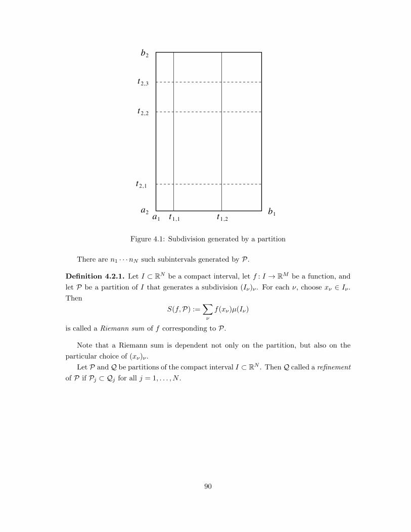
a1
a2 b1
b2
1 1 ,t t1 2,
2 1 ,t
2,2t
2 3,t
Figure 4.1: Subdivision generated by a partition
There are n1 · · ·nN such subintervals generated by P.
Definition 4.2.1. Let I ⊂ RN be a compact interval, let f : I → RM be a function, and
let P be a partition of I that generates a subdivision (Iν)ν . For each ν, choose xν ∈ Iν .
Then
S(f,P) :=∑ν
f(xν)µ(Iν)
is called a Riemann sum of f corresponding to P.
Note that a Riemann sum is dependent not only on the partition, but also on the
particular choice of (xν)ν .
Let P and Q be partitions of the compact interval I ⊂ RN . Then Q called a refinement
of P if Pj ⊂ Qj for all j = 1, . . . , N .
90

refinement of
Figure 4.2: Subdivisions corresponding to a partition and to a refinement
If P1 and P2 are any two partitions of I, there is always a common refinement Q of
P1 and P2.
2
1
21and
common refinement of
Figure 4.3: Subdivision corresponding to a common refinement
Definition 4.2.2. Let I ⊂ RN be a compact interval, let f : I → RM be a function,
and suppose that there is y ∈ RM with the following property: For each ε > 0, there is a
partition Pε of I such that, for each refinement P of Pε and for any Riemann sum S(f,P)
corresponding to P, we have ‖S(f,P)− y‖ < ε. Then f is said to be Riemann integrable
on I, and y is called the Riemann integral of f over I.
In the situation of Definition 4.2.2, we write
y =:
∫If =:
∫If dµ =:
∫If(x1, . . . , xN ) dµ(x1, . . . , xN ).
The proof of the following is an easy exercise:
91

Proposition 4.2.3. Let I ⊂ RN be a compact interval, and let f : I → RM be Riemann
integrable. Then∫I f is unique.
Theorem 4.2.4 (Cauchy Criterion for Riemann Integrability). Let I ⊂ RN be a compact
interval, and let f : I → RM be a function. Then the following are equivalent:
(i) f is Riemann integrable;
(ii) for each ε > 0, there is a partition Pε of I such that, for all refinements P and Qof Pε and for all Riemann sums S(f,P) and S(f,Q) corresponding to P and Q,
respectively, we have ‖S(f,P)− S(f,Q)‖ < ε.
Proof. (i) =⇒ (ii): Let y :=∫I f , and let ε > 0. Then there is a partition Pε of I such
that
‖S(f,P)− y‖ < ε
2
for all refinements P of Pε and for all corresponding Riemann sums S(f,P). Let P and Qbe any two refinements of Pε, and let S(f,P) and S(f,Q) be the corresponding Riemann
sums. Then we have
‖S(f,P)− S(f,Q)‖ ≤ ‖S(f,P)− y‖+ ‖S(f,Q)− y‖ < ε
2+ε
2= ε,
which proves (ii).
(ii) =⇒ (i): For each n ∈ N, there is a partition Pn of I such that
‖S(f,P)− S(f,Q)‖ < 1
2n
for all refinements P and Q of Pn and for all Riemann sums S(f,P) and S(f,Q) cor-
responding to P and Q, respectively. Without loss of generality suppose that Pn+1 is a
refinement of Pn. For each n ∈ N, fix a particular Riemann sum Sn := S(f,Pn). For
n > m, we then have
‖Sn − Sm‖ ≤n−1∑k=m
‖Sk+1 − Sk‖ <n−1∑k=m
1
2k,
so that (Sn)∞n=1 is a Cauchy sequence in RM . Let y := limn→∞ Sn. We claim that
y =∫Y f .
Let ε > 0, and choose n0 so large that 12n0 < ε
2 and ‖Sn0 − y‖ < ε2 . Let P be a
refinement of Pn0 , and let S(f,P) be a Riemann sum corresponding to P. Then we have
‖S(f,P)− y‖ ≤ ‖S(f,P)− Sn0‖︸ ︷︷ ︸< 1
2n0< ε
2
+ ‖Sn0 − y‖︸ ︷︷ ︸< ε
2
< ε.
This proves (i).
92

The Cauchy Criterion for Riemann Integrability has a somewhat surprising—and very
useful—corollary. For its proof, we require the following lemma of which the proof is
elementary, but unpleasant (and thus omitted):
Lemma 4.2.5. Let I ⊂ RN be a compact interval, and let P be a partiation of I subdi-
viding it into (Iν)ν . Then we have
µ(I) =∑ν
µ(Iν).
Corollary 4.2.6. Let I ⊂ RN be a compact interval, and let f : I → RM be a function.
Then the following are equivalent:
(i) f is Riemann integrable;
(ii) for each ε > 0, there is a partition Pε of I such that ‖S1(f,Pε)− S2(f,Pε)‖ < ε for
any two Riemann sums S1(f,Pε) and S2(f,Pε) corresponding to Pε.
Proof. (i) =⇒ (ii) is clear in the light of Theorem 4.2.4.
(i) =⇒ (i): Without loss of generality, suppose that M = 1.
Let (Iν)ν be the subdivions of I corresponding to Pε. Let P and Q be refinements of
Pε with subdivision (Jµ)µ and (Kλ)λ of I, respectively. Note that
S(f,P)− S(f,Q)
=∑µ
f(xµ)µ(Jµ)−∑λ
f(yλ)µ(Kλ) =∑ν
∑Jµ⊂Iν
f(xµ)µ(Jµ)−∑
Kλ⊂Iν
f(yλ)µ(Kλ)
.
For any index ν, choose z∗ν , zν∗ ∈ Iν such that
f(z∗ν) = max{f(xµ), f(yλ) : Jµ,Kλ ⊂ Iν}
and
f(zν∗) = min{f(xµ), f(yλ) : Jµ,Kλ ⊂ Iν}.
For ν, we obtain
(f(zν∗)− f(z∗ν))µ(Iν)
= f(zν∗)∑Jµ⊂Iν
µ(Jµ)− f(z∗ν)∑
Kλ⊂Iν
µ(Kλ), by Lemma 4.2.5,
≤∑Jµ⊂Iν
f(xµ)µ(Jµ)−∑
Kλ⊂Iν
f(yλ)µ(Kλ)
≤ f(z∗ν)∑Jµ⊂Iν
µ(Jµ)− f(zν∗)∑
Kλ⊂Iν
µ(Kλ)
= (f(z∗ν)− f(zν∗))µ(Iν), by Lemma 4.2.5 again,
93
so that ∣∣∣∣∣∣∑Jµ⊂Iν
f(xµ)µ(Jµ)−∑
Kλ⊂Iν
f(yλ)µ(Kλ)
∣∣∣∣∣∣ ≤ (f(z∗ν)− f(zν∗))µ(Iν).
It follows that
|S(f,P)− S(f,Q)|
≤∑ν
(f(z∗ν)− f(zν∗))µ(Iν) =
∣∣∣∣∣∑ν
f(z∗ν)µ(Iν)︸ ︷︷ ︸=S1(f,Pε)
−∑ν
f(zν∗)µ(Iν)︸ ︷︷ ︸=S2(f,Pε)
∣∣∣∣∣ < ε,
which completes the proof.
Theorem 4.2.7. Let I ⊂ RN be a compact interval, and let f : I → RM be continuous.
Then f is Riemann integrable.
Proof. Since I is compact, f is uniformly continuous.
Let ε > 0. Then there is δ > 0 such that ‖f(x) − f(y)‖ < εµ(I) for x, y ∈ I with
‖x− y‖ < δ.
Choose a partition P of I with the following property: If (Iν)ν is the subdivision of I
generated by P, then, for each
Iν := [a(ν)1 , b
(ν)1 ]× · · · × [a
(ν)N , b
(ν)N ],
we have
maxj=1,...,N
|a(ν)j − b
(ν)j | <
δ√N.
Let S1(f,P) and S2(f,P) be any two Riemann sums of f corresponding to P, namely
S1(f,P) =∑ν
f(xν)µ(Iν) and S2(f,P) =∑ν
f(yν)µ(Iν)
with xν , yν ∈ Iν . Hence,
‖xν − yν‖ =
√√√√ N∑j=1
(xν,j − yν,j)2 <
√√√√ N∑j=1
δ2
N= δ
holds, so that
‖S1(f,P)− S2(f,P)‖ ≤∑ν
‖f(xν)− f(yν)‖µ(Iν) <ε
µ(I)
∑ν
µ(Iν) = ε.
This completes the proof.
Our next theorem improves Theorem 4.2.8 and has a similar, albeit technically more
involved proof:
94

Theorem 4.2.8. Let I ⊂ RN be a compact interval, and let f : I → RM be bounded
such that S := {x ∈ I : f is discontinous at x} has content zero. Then f is Riemann
integrable.
Proof. Let C ≥ 0 be such that ‖f(x)‖ ≤ C for x ∈ I, and let ε > 0.
Choose a partition P of I such that∑Iν∩S 6=∅
µ(Iν) <ε
4(C + 1)
holds for the corresponding subdivision (Iν)ν of I, and let
K :=⋃
Iν∩S=∅Iν .
S
I
K
Figure 4.4: The idea of the proof of Theorem 4.2.8
Then K is compact, and f |K is continous; hence, f |K is uniformly continous.
Choose δ > 0 such that ‖f(x)− f(y)‖ < ε2µ(I) for x, y ∈ K with ‖x− y‖ < δ. Choose
a partition Q refining P such that, for each interval Jλ in the corresponding subdivision
(Jλ)λ of I with
Jλ := [a(λ)1 , b
(λ)1 ]× · · · × [a
(λ)N , b
(λ)N ],
we have
maxj=1,...,N
|a(λ)j − b
(λ)j | <
δ√N.
Let S1(f,Q) and S2(f,Q) be any two Riemann sums of f corresponding to Q, namely
S1(f,Q) =∑λ
f(xλ)µ(Jλ) and S2(f,Q) =∑λ
f(yλ)µ(Jλ).
95

It follows that
‖S1(f,Q)− S2(f,Q)‖ ≤∑λ
‖f(xλ)− f(yλ)‖µ(Jλ)
=∑Jλ 6⊂K
‖f(xλ)− f(yλ)‖︸ ︷︷ ︸≤2C
µ(Jλ) +∑Jλ⊂K
‖f(xλ)− f(yλ)‖︸ ︷︷ ︸< ε
2µ(I)
µ(Jλ)
≤ 2C∑Jλ 6⊂K
µ(Jλ) +ε
2µ(I)
∑Jλ⊂K
µ(Jλ)︸ ︷︷ ︸< ε
2
≤ 2C∑
Iν∩S 6=∅
µ(Iν)︸ ︷︷ ︸< ε
4(C+1)
+ε
2
<ε
2+ε
2
= ε,
which proves the claim.
Let ∅ 6= D ⊂ RN be bounded, and let f : D → RM be a function. Let I ⊂ RN be a
compact interval such that D ⊂ I. Define
f : I → RM , x 7→
{f(x), x ∈ D,
0, x /∈ D.(4.1)
We say that f is Riemann integrable on D if f is Riemann integrable on I. We define∫Df :=
∫If .
It is easy to see that this definition is independent of the choice of I.
Theorem 4.2.9. Let ∅ 6= D ⊂ RN be bounded with µ(∂D) = 0, and let f : D → RM be
bounded and continuous. Then f is Riemann integrable on D.
Proof. Define f as in (4.1). Then f is continuous at each point of int D as well as at each
point of int(I \D). Consequently,
{x ∈ I : f is discontinuous at x} ⊂ ∂D
has content zero. The claim then follows from Theorem 4.2.8.
Definition 4.2.10. Let D ⊂ RN be bounded. We say that D has content if 1 is Riemann
integrable on D. We write
µ(D) :=
∫D
1.
96

Sometimes, if we want to emphasize the dimension N , we write µN (D).
For any set S ⊂ RN , let its indicator function be
χS : RN → R, x 7→
{1, x ∈ S,0, x /∈ S.
If D ⊂ RN is bounded, and I ⊂ RN is a compact interval with D ⊂ I, then Definition
4.2.10 becomes
µ(D) =
∫IχD.
It is important not to confuse the statements “D does not have content” and “D has
content zero”: a set with content zero always has content.
The following theorem characterizes the sets that have content in terms of their bound-
aries:
Theorem 4.2.11. The following are equivalent for a bounded set D ⊂ RN :
(i) D has content.
(ii) ∂D has content zero.
Proof. (ii) =⇒ (i) is clear by Theorem 4.2.9.
(i) =⇒ (ii): Assume towards a contradiction that D has content, but that ∂D does
not have content zero. By Lemma 4.1.2, this means that there is ε0 > 0 such that, for any
compact intervals I1, . . . , In ⊂ RN with ∂D ⊂⋃nj=1 Ij , we have
n∑j=1
int Ij∩∂D 6=∅
µ(Ij) ≥ ε0.
Let I ⊂ RN be a compact interval such that D ⊂ I. Choose a partition P of I such that
|S(χD,P)− µ(D)| < ε02
for any Riemann sum of χD corresponding to P. Let (Iν)ν be the subdivision of I corre-
sponding to P. Choose support points xν ∈ Iν with xν ∈ D whenever int Iν ∩ ∂D 6= ∅.
Let
S1(χD,P) =∑ν
χD(xν)µ(Iν).
Choose support points yν ∈ Iν such that yν = xν if int Iν ∩ ∂D = ∅ and yν ∈ Dc if
int Iν ∩ ∂D 6= ∅, and let
S2(χD,P) =∑ν
χD(yν)µ(Iν).
97

It follows that
S1(χD,P)− S2(χD,P) =∑ν
(int Iν)∩∂D 6=∅
µ(Iν) ≥ ε0.
On the other hand, however, we have
|S1(χD,P)− S2(χD,P)| ≤ |S1(χD,P)− µ(D)|+ |S2(χD,P)− µ(D)| < ε0,
which is a contradiction.
Before go ahead and actually compute Riemann integrals, we sum up (and prove) a
few properties of the Riemann integral:
Proposition 4.2.12 (Properties of the Riemann Integral). The following are true:
(i) Let ∅ 6= D ⊂ RN be bounded, let f, g : D → RM be Riemann integrable on D, and
let λ, µ ∈ R. Then λf + µg is Riemann integrable on D such that∫D
(λf + µg) = λ
∫Df + µ
∫Dg.
(ii) Let ∅ 6= D ⊂ RN be bounded, and let f : D → R be non-negative and Riemann
integrable on D. Then∫D f is non-negative.
(iii) Let ∅ 6= D ⊂ RN be bounded, and let f : D → RM be Riemann integrable on D.
Then
‖f‖ : D → R, x 7→ ‖f(x)‖
is Riemannn integrable with ∥∥∥∥∫Df
∥∥∥∥ ≤ ∫D‖f‖.
(iv) Let D1, D2 ⊂ RN be non-empty and bounded such that µ(D1 ∩ D2) = 0, and let
f : D1 ∪ D2 → RM be Riemann integrable on D1 and D2. Then f is Riemann
integrable on D1 ∪D2 such that∫D1∪D2
f =
∫D1
f +
∫D2
f.
(v) Let ∅ 6= D ⊂ RN have content, let f : D → R be Riemann integrable, and let
m,M ∈ R be such that
m ≤ f(x) ≤M
for x ∈ D. Then
mµ(D) ≤∫Df ≤M µ(D)
holds.
98

(vi) Let ∅ 6= D ⊂ RN be compact, connected, and have content, and let f : D → R be
continuous. Then there is x0 ∈ D such that∫Df = f(x0)µ(D).
Proof. (i) is routine.
(ii): Without loss of generality, suppose that I is a compact interval. Assume that∫I f < 0. Let ε := −
∫I f > 0, and choose a partition P of I such that for all Riemann
sums S(f,P) corresponding to P, the inequality∣∣∣∣S(f,P)−∫If
∣∣∣∣ < ε
2
holds. It follows that
S(f,P) < − ε2< 0,
whereas, on the other hand,
S(f,P) =∑ν
f(xν)µ(Iν) ≥ 0,
where (Iν)ν is the subdivision of I corresponding to P.
(iii): Again, suppose that D is a compact interval I.
Let ε > 0, and let f1, . . . , fM denote the components of f . By Corollary 4.2.6, there
is a partition Pε of I such that
|S1(fj ,Pε)− S2(fj ,Pε)| <ε
M
for j = 1, . . . ,M and for all Riemann sums S1(fj ,Pε) and S2(fj ,Pε) corresponding to Pε.Let (Iν)ν be the subdivision of I induced by Pε. Choose support points xν , yν ∈ Iν . Fix
j ∈ {1, . . . ,M}. Let z∗ν , zν∗ ∈ {xν , yν} be such that
fj(z∗ν) = max{fj(xν), fj(yν)} and fj(zν∗) = min{fj(xν), fj(yν)}
We then have that∑ν
|fj(xν)− fj(yν)|µ(Iν)
=∑ν
(fj(z∗ν)− fj(zν∗))µ(Iν) =
∑ν
fj(z∗ν)µ(Iν)−
∑ν
fj(zν∗)µ(Iν) <ε
M.
99

It follows that∣∣∣∣∣∑ν
‖f(xν)‖µ(Iν)−∑ν
‖f(yν)‖µ(Iν)
∣∣∣∣∣ ≤∑ν
‖f(xν)− f(yν)‖µ(Iν)
≤∑ν
M∑j=1
|fj(xν)− fj(yν)|µ(Iν)
≤M∑j=1
∑ν
|fj(xν)− fj(yν)|µ(Iν)
< Mε
M
= ε,
so that ‖f‖ is Riemann integrable by the Cauchy criterion.
Let ε > 0 and choose a partition P of I with corresponding subdivision (Iν)ν of I and
support points xν ∈ Iν such that∥∥∥∥∥∑ν
f(xν)µ(Iν)−∫If
∥∥∥∥∥ < ε
2
and ∣∣∣∣∣∑ν
‖f(xν)‖µ(Iν)−∫I‖f‖
∣∣∣∣∣ < ε
2.
It follows that∥∥∥∥∫If
∥∥∥∥ ≤∥∥∥∥∥∑
ν
f(xν)µ(Iν)
∥∥∥∥∥+ε
2≤∑ν
‖f(xν)‖µ(Iν) +ε
2≤∫I‖f‖+ ε.
Since ε > 0 was arbitrary, this means that∥∥∫
I f∥∥ ≤ ∫I ‖f‖.
(iv): Choose a compact interval I ⊂ RN such that D1, D2 ⊂ I, and note that∫Dj
f =
∫IfχDj =
∫D1∪D2
fχDj
for j = 1, 2. In particular, fχD1 and fχD2 are Riemann integrable on D1 ∪ D2. Since
µ(D1 ∩D2) = 0, the function fχD1∩D2 is automatically Riemann integrable, so that
f = fχD1 + fχD2 − fχD1∩D2
is Riemann integrable. It follows from (i) that∫D1∪D2
f =
∫D1
f +
∫D2
f −∫D1∩D2
f︸ ︷︷ ︸=0
.
100

(v): Since M − f(x) ≥ 0 holds for all x ∈ D, we have by (ii) that
0 ≤∫D
(M − f) = M
∫D
1−∫Df = M µ(D)−
∫Df.
Similarly, one proves that mµ(D) ≤∫D f .
(vi): Without loss of generality, suppose that µ(D) > 0. Let
m := inf{f(x) : x ∈ D} and M := sup{f(x) : x ∈ D},
so that
m ≤∫D f
µ(D)≤M.
Let x1, x2 ∈ D be such that f(x1) = m and f(x2) = M . By the Intermediate Value
Theorem, there is x0 ∈ D such that f(x0) =∫D f
µ(D) .
Exercises
1. Let I be a compact interval, and let f = (f1, . . . , fM ) : I → RM . Show that f
is Riemann integrable if and only if fj : I → R is Riemann integrable for each
j = 1, . . . ,M and that, in this case,∫If =
(∫If1, . . . ,
∫IfM
)holds.
2. Let I ⊂ RN be a compact interval, and let f : I → RM be Riemann integrable.
Show that f is bounded.
3. Let ∅ 6= D ⊂ RN have content zero, and let f : D → RM be bounded. Show that f
is Riemann-integrable on D such that∫Df = 0.
4. Let ∅ 6= D ⊂ RN be bounded, and let f, g : D → R be Riemann-integrable. Show
that fg : D → R is Riemann-integrable.
Do we have ∫Dfg =
(∫Df
)(∫Dg
)?
(Hint : First treat the case where f = g, treat the general case by observing that
fg = 12((f + g)2 − f2 − g2.)
5. Let ∅ 6= U ⊂ RN be open with content, and let f : U → [0,∞) be bounded and
continuous such that∫U f = 0. Show that f ≡ 0 on U .
101

6. Let I ⊂ RN be a compact interval. Show that
A := {A ⊂ I : A has content}
is an algebra over I, i.e.,
(a) ∅, I ∈ A,
(b) if A ∈ A, then I \A ∈ A, and
(c) if A1, . . . , An ∈ A, then A1 ∪ · · · ∪An ∈ A.
4.3 Evaluation of Integrals in One Variable: A Review
In this section, we review the basic techniques for evaluating Riemann integrals of func-
tions of one variable:
Theorem 4.3.1. Let f : [a, b]→ R be continous, and let F : [a, b]→ R be defined as
F (x) :=
∫ x
af(t) dt
for x ∈ [a, b]. Then F is an antiderivative of f , i.e., F is differentiable such that F ′ = f .
Proof. Let x ∈ [a, b], and let h 6= 0 such that x+ h ∈ [a, b]. By the Mean Value Theorem
of integration, we obtain that
F (x+ h)− F (x) =
∫ x+h
xf(t) dt = f(ξh)h
for some ξh between x+ h and x. It follows that
F (x+ h)− F (x)
h= f(ξh)
h→0→ f(x)
because f is continuous.
Proposition 4.3.2. Let F1 and F2 be antiderivatives of a function f : [a, b] → R. Then
F1 − F2 is constant.
Proof. This is clear because (F1 − F2)′ = f − f = 0.
Theorem 4.3.3 (Fundamental Theorem of Calculus). Let f : [a, b] → R be continuous,
and let F : [a, b]→ R be any antiderivative of f . Then∫ b
af(x) dx = F (b)− F (a) =: F (x)
∣∣∣ba
holds.
102

Proof. By Theorem 4.3.1 and by Proposition 4.3.2, there is C ∈ R such that∫ x
af(t) dt = F (x)− C
for all x ∈ [a, b]. Since
F (a)− C =
∫ a
af(t) dt = 0,
we have C = F (a) and thus ∫ b
af(t) dt = F (b)− F (a).
This proves the claim.
Example. Since ddx sinx = cosx, it follows that∫ π
0sinx dx = − cosx
∣∣∣π0
= 2.
Corollary 4.3.4 (Change of Variables). Let φ : [a, b]→ R be continuously differentiable,
let f : [c, d]→ R be continuous, and suppose that φ([a, b]) ⊂ [c, d]. Then∫ φ(b)
φ(a)f(x) dx =
∫ b
af(φ(t))φ′(t) dt
holds.
Proof. Let F be an antiderivative of f . The chain rule yields that
(F ◦ φ)′ = (f ◦ φ)φ′,
so that F ◦ φ is an antiderivative of (f ◦ φ)φ′. By the fundamental theorem of calculus,
we thus have∫ φ(b)
φ(a)f(x) dx = F (φ(b))− F (φ(a)) = (F ◦ φ)(b)− (F ◦ φ)(b) =
∫ b
af(φ(t))φ′(t) dt
as claimed.
Examples. 1. We have ∫ √π0
x sin(x2) dx =1
2
∫ √π0
2x sin(x2) dx
=1
2
∫ π
0sinu du
= −1
2cosu
∣∣∣∣π0
=1
2+
1
2
= 1.
103

2. We have∫ 1
0
√1− x2 dx =
∫ π2
0
√1− sin2 t cos t dt =
∫ π2
0
√cos2 t cos t dt =
∫ π2
0cos2 t dt.
Corollary 4.3.5 (Integration by Parts). Let f, g : [a, b]→ R be continuously differentiable.
Then ∫ b
af(x)g′(x) dx = f(b)g(b)− f(a)g(a)−
∫ b
af ′(x)g(x) dx
holds.
Proof. By the product rule, we have
d
dxf(x)g(x) = f(x)g′(x) + f ′(x)g(x)
for x ∈ [a, b], and the fundamental theorem of calculus yields
f(b)g(b)− f(a)g(a) =
∫ b
a
d
dxf(x)g(x) dx
=
∫ b
a(f(x)g′(x) + f ′(x)g(x)) dx
=
∫ b
af(x)g′(x) dx+
∫ b
af ′(x)g(x) dx
as claimed.
Examples. 1. Note that∫ π2
0cos2 x dx = − sin(0) cos(0) + sin
(π2
)cos(π
2
)+
∫ π2
0sin2 x dx
=
∫ π2
0sin2 x dx
=
∫ π2
0(1− cos2 x) dx
=π
2−∫ π
2
0cos2 x dx,
so that ∫ π2
0cos2 x dx =
π
4.
Combining this with the second example on change of variables, we also obtain that∫ 1
0
√1− t2 dt =
∫ π2
0cos2 x dx =
π
4.
104
2. We have∫ x
1log t dt =
∫ x
11 log t dt = t log t
∣∣∣x1−∫ x
1t1
tdt = x log x− (x− 1).
Hence,
(0,∞)→ R, x 7→ x log x− x
is an antiderivative of the natural logarithm.
4.4 Fubini’s Theorem
Fubini’s Theorem is the first major tool for the actual computation of Riemann inte-
grals in several dimensions (the other one is Change of Variables). It asserts that multi-
dimensional Riemann integrals can be computed through iteration of one-dimensional
ones:
Theorem 4.4.1 (Fubini’s Theorem). Let I ⊂ RN and J ⊂ RM be compact intervals, and
let f : I × J → RK be Riemann integrable such that, for each x ∈ I, the integral
F (x) :=
∫Jf(x, y) dµM (y)
exists. Then F : I → RK is Riemann integrable such that∫IF =
∫I×J
f.
Proof. Let ε > 0.
Choose a partition Pε of I × J such that∥∥∥∥S(f,P)−∫I×J
f
∥∥∥∥ < ε
2
for any Riemann sum S(f,P) of f corresponding to a partition P of I × J finer than Pε.Let Pε,x and Pε,y be the partitions of I and J , respectively, such that Pε := Pε,x×Pε,y.
Set Qε := Pε,x, and let Q be a refinement of Qε with corresponding subdivision (Iν)ν of
I; pick xν ∈ Iν . For each ν, there is a partition Rε,ν of J such that, for each refinement
R of Rε,ν with corresponding subdivision (Jλ)λ, we have∥∥∥∥∥∑λ
f(xν , yλ)µM (Jλ)− F (xν)
∥∥∥∥∥ < ε
2µN (I)(4.2)
for any choice of yλ ∈ Jλ. Let Rε be a common refinement of (Rε,ν)ν and Pε,y with
corresponding subdivision (Jλ)λ of J . Consequently, Q × Rε is a refinement of Pε with
corresponding subdivision (Iν × Jλ)λ,ν of I × J . Picking yλ ∈ Jλ, we thus have∥∥∥∥∥∥∑ν,λ
f(xν , yλ)µN (Iν)µM (Jλ)−∫I×J
f
∥∥∥∥∥∥ < ε
2. (4.3)
105

We therefore obtain∥∥∥∥∥∑ν
F (xν)µN (Iν)−∫I×J
f
∥∥∥∥∥≤
∥∥∥∥∥∥∑ν
F (xν)µN (Iν)−∑ν,λ
f(xν , yλ)µN (Iν)µM (Jλ)
∥∥∥∥∥∥+
∥∥∥∥∥∥∑ν,λ
f(xν , yλ)µN (Iν)µM (Jλ)−∫I×J
f
∥∥∥∥∥∥<
∥∥∥∥∥∥∑ν
F (xν)µN (Iν)−∑ν,λ
f(xν , yλ)µN (Iν)µM (Jλ)
∥∥∥∥∥∥+ε
2, by (4.3),
≤∑ν
∥∥∥∥∥F (xν)−∑λ
f(xν , yλ)µM (Jλ)
∥∥∥∥∥µN (Iν) +ε
2
<∑ν
ε
2µN (I)µ(Iν) +
ε
2
=ε
2+ε
2
= ε.
Since this holds for each refinement Q of Qε, and for any choice of xν ∈ Iν , we obtain
that F is Riemann integrable such that∫IF =
∫I×J
f,
as claimed.
Examples. 1. Let
f : [0, 1]× [0, 1]→ R, (x, y) 7→ xy.
We obtain ∫[0,1]×[0,1]
f =
∫ 1
0
(∫ 1
0xy dy
)dx
=
∫ 1
0x
(∫ 1
0y dy
)dx
=
∫ 1
0x
(y2
2
∣∣∣∣10
)dx
=1
2
∫ 1
0x dx
=1
4.
106

2. Let
f : [0, 1]× [0, 1]→ R, (x, y) 7→ y3exy2.
Then Fubini’s Theorem yields∫[0,1]×[0,1]
f =
∫ 1
0
(∫ 1
0y3exy
2dy
)dx =?.
Changing the order of integration, however, we obtain∫[0,1]×[0,1]
f =
∫ 1
0
(∫ 1
0y3exy
2dx
)dy
=
∫ 1
0yexy
2∣∣∣10dy
=
∫ 1
0(yey
2 − y) dy
=1
2ey
2 − y2
2
∣∣∣∣10
=1
2e− 1
2− 1
2
=1
2e− 1.
The following corollary is a straightforward specialization of Fubini’s Theorem applied
twice (in each variable).
Corollary 4.4.2. Let I = [a, b]× [c, d], let f : I → R be Riemann integrable, and suppose
that:
(a) for each x ∈ [a, b], the integral∫ dc f(x, y) dy exists;
(b) for each y ∈ [c, d], the integral∫ ba f(x, y) dx exists.
Then ∫ b
a
(∫ d
cf(x, y) dy
)dx =
∫If =
∫ d
c
(∫ b
af(x, y) dx
)dy
holds.
Similarly straightforward is the next corollary:
Corollary 4.4.3. Let I = [a, b]× [c, d], and let f : I → R be bounded such that the set D0
of its discontinuity points has content zero and satisfies µ1({y ∈ [c, d] : (x, y) ∈ D0}) = 0
for each x ∈ [a, b]. Then f is Riemann integrable such that∫If =
∫ b
a
(∫ d
cf(x, y) dy
)dx.
107
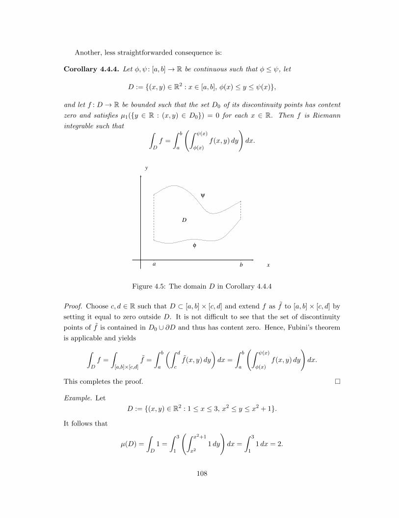
Another, less straightforwarded consequence is:
Corollary 4.4.4. Let φ, ψ : [a, b]→ R be continuous such that φ ≤ ψ, let
D := {(x, y) ∈ R2 : x ∈ [a, b], φ(x) ≤ y ≤ ψ(x)},
and let f : D → R be bounded such that the set D0 of its discontinuity points has content
zero and satisfies µ1({y ∈ R : (x, y) ∈ D0}) = 0 for each x ∈ R. Then f is Riemann
integrable such that ∫Df =
∫ b
a
(∫ ψ(x)
φ(x)f(x, y) dy
)dx.
y
xba
φ
ψ
D
Figure 4.5: The domain D in Corollary 4.4.4
Proof. Choose c, d ∈ R such that D ⊂ [a, b] × [c, d] and extend f as f to [a, b] × [c, d] by
setting it equal to zero outside D. It is not difficult to see that the set of discontinuity
points of f is contained in D0 ∪ ∂D and thus has content zero. Hence, Fubini’s theorem
is applicable and yields∫Df =
∫[a,b]×[c,d]
f =
∫ b
a
(∫ d
cf(x, y) dy
)dx =
∫ b
a
(∫ ψ(x)
φ(x)f(x, y) dy
)dx.
This completes the proof.
Example. Let
D := {(x, y) ∈ R2 : 1 ≤ x ≤ 3, x2 ≤ y ≤ x2 + 1}.
It follows that
µ(D) =
∫D
1 =
∫ 3
1
(∫ x2+1
x21 dy
)dx =
∫ 3
11 dx = 2.
108
Corollary 4.4.5 (Cavalieri’s Principle). Let N ≥ 2, and suppose that S, T ⊂ RN have
content. For each x ∈ R, let
Sx := {(x1, . . . , xN−1) ∈ RN−1 : (x, x1, . . . , xN−1) ∈ S}
and
Tx := {(x1, . . . , xN−1) ∈ RN−1 : (x, x1, . . . , xN−1) ∈ T},
and suppose that Sx and Tx have content with µN−1(Sx) = µN−1(Tx) for each x ∈ R.
Then µN (S) = µN (T ) holds.
Proof. Let I ⊂ R and J ⊂ RN−1 be compact intervals such that S, T ⊂ I × J , and note
that
µN (S) =
∫I×J
χS
=
∫I
(∫JχS(x, x1, . . . , xN−1) dµN−1(x1, . . . , xN−1)
)dx
=
∫I
(∫JχSx
)=
∫IµN−1(Sx)
=
∫IµN−1(Tx)
=
∫I
(∫JχTx
)=
∫I
(∫JχT (x, x1, . . . , xN−1) dµN−1(x1, . . . , xN−1)
)dx
=
∫I×J
χT
= µN (T ).
This completes the proof.
Example. Let r > 0, and let
T := {(x, y, z) ∈ R3 : z ≥ 0, x2 + y2 + z2 ≤ r2},
i.e., the half of Br[(0, 0, 0)] lying above the xy-plane, and
S := {(x, y, z) ∈ R3 : z ≥ 0, x2 + y2 ≤ r2, 0 ≤ z2 ≤ x2 + y2},
i.e., the part of the cylinder standing perpendicularly on the xy-plane with base Br[(0, 0)]
between the xy-plane and the plane z = r with the cone with base Br[(0, 0, r)] and apex
(0, 0, 0) removed.
109
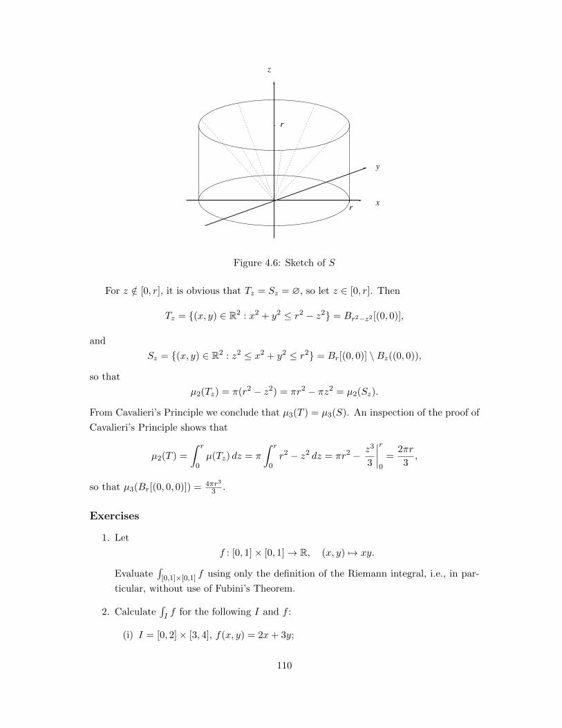
y
x
z
r
r
Figure 4.6: Sketch of S
For z /∈ [0, r], it is obvious that Tz = Sz = ∅, so let z ∈ [0, r]. Then
Tz = {(x, y) ∈ R2 : x2 + y2 ≤ r2 − z2} = Br2−z2 [(0, 0)],
and
Sz = {(x, y) ∈ R2 : z2 ≤ x2 + y2 ≤ r2} = Br[(0, 0)] \Bz((0, 0)),
so that
µ2(Tz) = π(r2 − z2) = πr2 − πz2 = µ2(Sz).
From Cavalieri’s Principle we conclude that µ3(T ) = µ3(S). An inspection of the proof of
Cavalieri’s Principle shows that
µ2(T ) =
∫ r
0µ(Tz) dz = π
∫ r
0r2 − z2 dz = πr2 − z3
3
∣∣∣∣r0
=2πr
3,
so that µ3(Br[(0, 0, 0)]) = 4πr3
3 .
Exercises
1. Let
f : [0, 1]× [0, 1]→ R, (x, y) 7→ xy.
Evaluate∫
[0,1]×[0,1] f using only the definition of the Riemann integral, i.e., in par-
ticular, without use of Fubini’s Theorem.
2. Calculate∫I f for the following I and f :
(i) I = [0, 2]× [3, 4], f(x, y) = 2x+ 3y;
110
(ii) I =[0, π2
]×[0, π2
], f(x, y) = sin(x+ y);
(iii) I = [1, 2]× [2, 3]× [0, 2], f(x, y, z) = 2z(x+y)2
.
3. Let a < b, let f : [a, b]→ [0,∞) be continuous, and let
D := {(x, y) : x ∈ [a, b], y ∈ [0, f(x)]}.
Show that D has content and that
µ(D) =
∫ b
af(x) dx.
4. Let
D := {(x, y) ∈ R : x, y ≥ 0, x2 + y2 ≤ 1},
and let
f : D → R, (x, y) 7→ 4y3
(x+ 1)2
Evaluate∫D f .
5. Define
f : [0, 1]3 → R, (x, y, z) 7→
{xy, z ≤ xy,z, z ≥ xy.
Evaluate∫
[0,1]3 f .
6. Let I ⊂ RN and J ⊂ RM be compact intervals, let f : I → R and g : J → R be
continuous, and define
f ⊗ g : I × J → R, (x, y) 7→ f(x)g(y).
7. Let f : [a, b]→ (0,∞) be continuous. Show that(∫ b
af(x) dx
)(∫ b
a
1
f(x)dx
)≥ (b− a)2.
(Hint : Apply Fubini’s Theorem to [a, b]2 3 (x, y) 7→ f(x)f(y) .)
8. Define f : [0, 1]× [0, 1]→ R by letting
f(x, y) =
22n, if (x, y) ∈ [2−n, 2−n+1)× [2−n, 2−n+1) for some n ∈ N,−22n+1, if (x, y) ∈ [2−n−1, 2−n)× [2−n, 2−n+1) for some n ∈ N,
0, otherwise.
Show that the iterated integrals∫ 1
0
(∫ 1
0f(x, y) dy
)dx and
∫ 1
0
(∫ 1
0f(x, y) dx
)dy
111
both exist, but that∫ 1
0
(∫ 1
0f(x, y) dy
)dx 6=
∫ 1
0
(∫ 1
0f(x, y) dx
)dy.
Why doesn’t this contradict Fubini’s Theorem?
4.5 Integration in Polar, Spherical, and Cylindrical Coor-
dinates
In the last example of the previous section, we used Fubini’s Theorem to determine the
volume of a sphere in R3—by making recourse to the area of a disc in R2. But how can
we rigorously compute the are of a disc with given diameter in R2? We will answer this
question in this section.
The second main tool for the calculation of multi-dimensional integrals is the multi-
dimensional Change of Variables formula:
Theorem 4.5.1 (Change of Variables). Let ∅ 6= U ⊂ RN be open, let ∅ 6= K ⊂ U be
compact with content, let φ : U → RN be continuously partially differentiable, and suppose
that there is a set Z ⊂ K with content zero such that φ|K\Z is injective and det Jφ(x) 6= 0
for all x ∈ K \ Z. Then φ(K) has content and∫φ(K)
f =
∫K
(f ◦ φ)| det Jφ|
holds for all continuous functions f : φ(U)→ RM .
Proof. Postponed, but not skipped!
Examples. 1. Let a, b, c > 0 and let
E :=
{(x, y, z) ∈ R3 :
x2
a2+y2
b2+z2
c2≤ 1
}.
What is the content of E?
Let
φ : R3 → R3, (r, θ, σ) 7→ (ar cos θ cosσ, br cos θ sinσ, cr sin θ),
and let
K := [0, 1]×[−π
2,π
2
]× [0, 2π],
so that E = φ(K). Of course, φ is not injective on K.
112
Set
Z :=({0} ×
[−π
2,π
2
]× [0, 2π]
)∪(
[0, 1]×{−π
2,π
2
}× [0, 2π]
)∪(
[0, 1]×[−π
2,π
2
]× {0}
),
so that
K \ Z = (0, 1]×(−π
2,π
2
)× (0, 2π].
It is clear that µ3(Z) = 0.
We claim that φ|K\Z is injective. To see this, let (r1, θ1, σ1), (r2, θ2, σ2) ∈ K \ Z be
such that φ(r1, θ1, σ1) = φ(r2, θ2, σ2). As a, b, c > 0, this means that
r1 cos θ1 cosσ1 = r2 cos θ2 cosσ2,
r1 cos θ1 sinσ1 = r2 cos θ2 sinσ2, and r1 sin θ1 = r2 sin θ2.
It follows that
r21 = r2
1(cos2 θ1(cos2 σ1 + sin2 σ1) + sin2 θ1)
= r21 cos2 θ1 cos2 σ1 + r2
1 cos2 θ1 sin2 σ1 + r21 sin2 θ1
= r22 cos2 θ2 cos2 σ2 + r2
2 cos2 θ2 sin2 σ2 + r22 sin2 θ2
= r22(cos2 θ2(cos2 σ2 + sin2 σ2) + sin2 θ2)
= r22,
so that r1 = r2. As r1, r2 > 0, this means that
cos θ1 cosσ1 = cos θ2 cosσ2,
cos θ1 sinσ1 = cos θ2 sinσ2, and sin θ1 = sin θ2.
Now, sin is injective on[−π
2 ,π2
], so that θ1 = θ2 and—consequently—cos θ1 = cos θ2.
As cos is non-zero on(−π
2 ,π2
), we conclude that
cosσ1 = cosσ2 and sinσ1 = sinσ2.
Since
(0, 2π]→ R2, σ 7→ (cosσ, sinσ)
is injective, it follows that σ1 = σ2 as well.
For (r, θ, σ) ∈ K, we have
Jφ(r, θ, σ) =
a cos θ cosσ, −ar sin θ cosσ, −ar cos θ sinσ
b cos θ sinσ, −br sin θ sinσ, br cos θ cosσ
c sin θ, cr cos θ, 0
,113

and thus
det Jφ(r, θ, σ) = abc det
cos θ cosσ, −r sin θ cosσ, −r cos θ sinσ
cos θ sinσ, −r sin θ sinσ, r cos θ cosσ
sin θ, r cos θ, 0
= abc
(sin θ
[−r sin θ cosσ, −r cos θ sinσ
−r sin θ sinσ, r cos θ cosσ
]
− r cos θ
[cos θ cosσ, −r cos θ sinσ
cos θ sinσ, r cos θ cosσ
])= −abc r2
(sin θ
((sin θ)(cos θ)(cos2 σ) + (sin θ)(cos θ)(sin2 σ)
)+ cos θ ((cos2 θ)(cos2 σ) + (cos2 θ)(sin2 σ))
)= −abc r2 cos θ
((sin2 θ)(cos2 σ) + (sin2 θ)(sin2 σ) + cos2 θ)
)= −abc r2 cos θ
(sin2 θ + cos2 θ
)= −abc r2 cos θ,
so that, particular, det Jφ(r, θ, σ) 6= 0 if (r, θ, σ) /∈ Z.
Therefore, Change of Variables applies, and we obtain
µ(E) =
∫E
1
=
∫K
1 |det Jφ|
= abc
∫ 1
0
(∫ π2
−π2
(∫ 2π
0r2 cos θ dσ
)dθ
)dr
= 2π abc
∫ 1
0r2
(∫ π2
−π2
cos θ dθ
)dr
= 2π abc
∫ 1
0r2 sin θ
∣∣π2−π
2dr
= 4π abc
∫ 1
0r2 dr
= 4π abcr3
3
∣∣∣∣10
=4π
3abc.
2. Let
f : R2 → R, (x, y) 7→ 1
x2 + y2 + 1.
Find∫B1[(0,0)] f .
114

Use polar coordinates, i.e., let
φ : R2 → R2, (r, θ) 7→ (r cos θ, r sin θ).
(x y),x
y
r
θ
Figure 4.7: Polar coordinates
It follows that B1[(0, 0)] = φ(K), where K = [0, 1]× [0, 2π]. We have
Jφ(r, θ) =
[cos θ, −r sin θ
sin θ, r cos θ
]
and thus
det Jφ(r, θ) = r.
Set
Z := ({0} × [0, 2π]) ∪ ([0, 1]× {0}),
so that Z has content zero, φ|K\Z is injective, and det Jφ is non-zero on K \ Z.
115

Change of Variables then yields∫B1[(0,0)]
f =
∫K
r
r2 + 1
=
∫ 1
0
(∫ 2π
0
r
r2 + 1dθ
)dr
= 2π
∫ 1
0
r
r2 + 1dr
= π
∫ 1
0
2r
r2 + 1dr
= π
∫ 2
1
1
sds
= π log s|21= π log 2.
3. Let
f : R3 → R, (x, y, z)→√x2 + y2 + z2,
and let R > 0.
Find∫BR[(0,0,0)] f .
Use spherical coordinates, i.e., let
φ : R3 → R3, (r, θ, σ) 7→ (r cos θ cosσ, r cos θ sinσ, r sin θ),
so that
det Jφ(r, θ, σ) = −r2 cos θ.
(x ,y ,z )
r
z
x
θ
σ
y
Figure 4.8: Spherical coordinates
116

It is clear that BR[(0, 0, 0)] = φ(K), where K = [0, R]×[−π
2 ,π2
]× [0, 2π]. Define Z
as in the first example. By Change of Variables, we thus have∫BR[(0,0,0)]
f =
∫Kr3 cos θ
=
∫ R
0
(∫ π2
−π2
(∫ 2π
0r3 cos θ dσ
)dθ
)dr
= 2π
∫ R
0
(r3
∫ π2
−π2
cos θ dθ
)dr
= 4π
∫ R
0r3 dr
= 4πr4
4
∣∣∣∣R0
= πR4.
4. Let
D := {(x, y, z) ∈ R3 : x, y ≥ 0, 1 ≤ z ≤ x2 + y2 ≤ e2},
and let
f : D → R, (x, y, z) 7→ 1
(x2 + y2)z.
Compute∫D f .
Use cylindrical coordinates, i.e., let
φ : R3 → R3, (r, θ, z) 7→ (r cos θ, r sin θ, z),
so that
Jφ(r, θ, z) =
cos θ, −r sin θ, 0
sin θ, r cos θ, 0
0, 0, 1
and
det Jφ(r, θ, z) = r.
117

(x y ,z ),
r
x
y
z
θ
Figure 4.9: Cylindrical coordinates
It follows that D = φ(K), where
K :={
(r, θ, z) : r ∈ [1, e], θ ∈[0,π
2
], z ∈ [1, r2]
}.
It is clear that φ is injective on K and that detJφ doesn’t vanish there. We thus
obtain ∫Df =
∫K
r
r2z
=
∫ e
1
(∫ π2
0
(∫ r2
1
1
rzdz
)dθ
)dr
=π
2
∫ e
1
(1
r
∫ r2
1
1
zdz
)dr
=π
2
∫ e
1
2 log r
rdr
= π
∫ 1
0s ds
=π
2.
5. Let R > 0, and let
C := {(x, y, z) ∈ R3 : x2 + y2 ≤ R2}
and
B := {(x, y, z) ∈ R3 : x2 + y2 + z2 ≤ 4R2}.
Find µ(C ∩B).
118

2R x
y
z
R
Figure 4.10: Intersection of ball and cylinder
Note that
µ(C ∩B) = 2(µ(D1) + µ(D2)),
where
D1 :={
(x, y, z) ∈ R3 : x2 + y2 + z2 ≤ 4R2, z ≥√
3(x2 + y2)}
and
D2 :={
(x, y, z) ∈ R3 : x2 + y2 ≤ R2, 0 ≤ z ≤√
3(x2 + y2)}.
Use spherical coordinates to compute µ(D1).
Note that D1 = φ(K1), where
K1 = [0, 2R]×[π
3,π
2
]× [0, 2π].
We obtain
µ(D1) =
∫K1
r2 cos θ
=
∫ 2R
0
(∫ π2
π3
(∫ 2π
0r2 cos θ dσ
)dθ
)dr
= 2π
∫ 2R
0
(r2
∫ π2
π3
cos θ dθ
)dr
= 2π
∫ 2R
0r2(
sin(π
2
)− sin
(π3
))dr
= 2π
(1−√
3
2
)∫ 2R
0r2 dr
=8R3
3π(2−
√3).
119
Use cylindrical coordinates to compute µ(D2), and note that D2 = φ(K2), where
K2 ={
(r, θ, z) : r ∈ [0, R], θ ∈ [0, 2π], z ∈[0,√
3 r]}
.
We obtain
µ(D2) =
∫K2
r
=
∫ R
0
(∫ 2π
0
(∫ √3 r
0r dz
)dθ
)dr
= 2π√
3
∫ R
0r2 dr
=2√
3R3
3π.
All in all, we have
µ(B ∩ C) = 2(µ(D1) + µ(D2))
=16R3
3π(2−
√3) +
4√
3R3
3π
=32R3
3π − 16
√3R3
3π +
4√
3R3
3π
=
(32
3− 4√
3
)πR3.
Exercises
1. Let a, b > 0. Determine the area of the ellipse
E :=
{(x, y) ∈ R2 :
x2
a2+y2
b2≤ 1
}.
2. Let D ⊂ R3 be the region in the first octant, i.e., with x, y, z ≥ 0, which is bounded
by the cylinder given by x2 + y2 = 16 and the plane given by z = 3. Evaluate∫Dxyz.
3. Let R > 0, and define, for 0 < ρ < R,
Aρ,R := {(x, y, z) ∈ R3 : ρ2 ≤ x2 + y2 + z2 ≤ R2}.
Determine
limρ→0
∫Aρ,R
1√x2 + y2 + z2
.
120
4. Let D in spherical coordinates be given as the solid lying between the spheres given
by r = 2 and r = 4, above the xy-plane and below the cone given by the angle
θ = π3 . Evaluate the integral
∫D xyz.
5. Let D ⊂ R2 be the trapeze with vertices (1, 0), (2, 0), (0,−2), and (0,−1). Evaluate∫D exp
(x+yx−y
). (Hint : Consider
φ : R2 → R2, (u, v) 7→(
1
2(u+ v),
1
2(u− v)
)and apply Change of Variables.)
121
Chapter 5
The Implicit Function Theorem
and Applications
5.1 Local Properties of C1-Functions
In this section, we study “local” properties of certain functions, i.e., properties that hold
if the function is restricted to certain subsets of its domain, but not necessarily for the
function on its whole domain.
We start this section with introducing some “shorthand” notation:
Definition 5.1.1. Let ∅ 6= U ⊂ RN be open. We call f : U → RM to be:
(a) of class C0—in symbols: f ∈ C0(U,RM )—if f is continuos;
(b) of class Cp with p ∈ N—in symbols: f ∈ Cp(U,RM )—if f is p times continuously
partially differentiable, i.e., all partial derivatives of f up to order p exist on U and
are continuous.
Our first local property is the following:
Definition 5.1.2. Let ∅ 6= D ⊂ RN , and let f : D → RM . Then f is locally injective at
x0 ∈ D if there is a neighborhood U of x0 such that f is injective on U ∩D. If f is locally
injective each point of U , we simply call f locally injective on D.
Trivially, every injective function is locally injective. But what about the converse?
Lemma 5.1.3. Let ∅ 6= U ⊂ RN be open, and let f ∈ C1(U,RN ) be such that det Jf (x0) 6=0 for some x0 ∈ U . Then f is locally injective at x0.
Proof. Choose ε > 0 such that Bε(x0) ⊂ U and
det
∂f1∂x1
(x(1)
), . . . , ∂f1
∂xN
(x(1)
)...
. . ....
∂fN∂x1
(x(N)
), . . . , ∂fN
∂xN
(x(N)
) 6= 0
122

for all x(1), . . . , x(N) ∈ Bε(x0).
Choose x, y ∈ Bε(x0) such that f(x) = f(y), and let ξ := y − x. By Taylor’s theorem,
there is, for each j = 1, . . . , N , a number θj ∈ [0, 1] such that
fj(x+ ξ︸ ︷︷ ︸=y
) = fj(x) +N∑k=1
∂fj∂xk
(x+ θjξ)ξk = fj(x).
It follows thatN∑k=1
∂fj∂xk
(x+ θjξ)ξk = 0
for j = 1, . . . , N . Let
A :=
∂f1∂x1
(x+ θ1ξ) , . . . , ∂f1∂xN
(x+ θ1ξ)...
. . ....
∂fN∂x1
(x+ θNξ) , . . . , ∂fN∂xN
(x+ θNξ)
,so that Aξ = 0. On the other hand, detA 6= 0 holds, so that ξ = 0, i.e., x = y.
Theorem 5.1.4. Let ∅ 6= U ⊂ RN be open, let M ≥ N , and let f ∈ C1(U,RM ) be such
that rank Jf (x) = N for all x ∈ U . Then f is locally injective on U .
Proof. Let x0 ∈ U . Without loss of generality suppose that
rank
∂f1∂x1
(x0), . . . , ∂f1∂xN
(x0)...
. . ....
∂fN∂x1
(x0), . . . , ∂fN∂xN
(x0)
= N.
Let f := (f1, . . . , fN ). It follows that
Jf (x) =
∂f1∂x1
(x), . . . , ∂f1∂xN
(x)...
. . ....
∂fN∂x1
(x), . . . , ∂fN∂xN
(x)
for x ∈ U and, in particular, detJf (x0) 6= 0.
By Lemma 5.1.3, f—and hence f—is therefore locally injective at x0.
Example. The function
f : R→ R2, x 7→ (cosx, sinx)
satisfies the hypothesis of Theorem 5.1.4 and thus is locally injective. Nevertheless,
f(x+ 2π) = f(x)
holds for all x ∈ R, so that f is not injective.
123
Next, we turn to an application of local injectivity:
Lemma 5.1.5. Let ∅ 6= U ⊂ RN be open, and let f ∈ C1(U,RN ) be such that det Jf (x) 6=0 for x ∈ U . Then f(U) is open.
Proof. Fix y0 ∈ f(U), and let x0 ∈ U be such that f(x0) = y0.
Choose δ > 0 such that Bδ[x0] ⊂ U and such that f is injective on Bδ[x0] (the latter is
possible by Lemma 5.1.3). Since f(∂Bδ[x0]) is compact and does not contain y0, we have
that
ε :=1
3inf{‖y0 − f(x)‖ : x ∈ ∂Bδ[x0]} > 0.
We claim that Bε(y0) ⊂ f(U).
Fix y ∈ Bε(y0), and define
g : Bδ[x0]→ R, x 7→ ‖f(x)− y‖2.
Then g is continuous, and thus attains its minimum at some x ∈ Bδ[x0]. Assume towards
a contradiction that x ∈ ∂Bδ[x0]. It then follows that√g(x) = ‖f(x)− y‖ ≥ ‖f(x)− y0‖︸ ︷︷ ︸
≥3ε
−‖y0 − y‖︸ ︷︷ ︸<ε
≥ 2ε > ε > ‖f(x0)− y‖ =√g(x0),
and thus g(x) > g(x0), which is a contradiction. It follows that x ∈ Bδ(x0).
Consequently, ∇g(x) = 0 holds. Since
g(x) =N∑j=1
(fj(x)− yj)2
for x ∈ Bδ[x0], it follows that
∂g
∂xk(x) = 2
N∑j=1
∂fj∂xk
(x)(fj(x)− yj)
holds for k = 1, . . . , N and x ∈ Bδ(x0). In particular, we have
0 =
N∑j=1
∂fj∂xk
(x)(fj(x)− yj)
for k = 1, . . . , N , and therefore
Jf (x)f(x) = Jf (x)y,
so that f(x) = y. It follows that y = f(x) ∈ f(Bδ(x0)) ⊂ f(U).
Theorem 5.1.6. Let ∅ 6= U ⊂ RN be open, let M ≤ N , and let f ∈ C1(U,RM ) with
rank Jf (x) = M for x ∈ U . Then f(U) is open.
124
Proof. Let x0 = (x0,1, . . . , x0,N ) ∈ U . We need to show that f(U) is a neighborhood of
f(x0). Without loss of generality suppose that
det
∂f1∂x1
(x0), . . . , ∂f1∂xM
(x0)...
. . ....
∂fM∂x1
(x0), . . . , ∂fM∂xM
(x0)
6= 0
and—making U smaller if necessary—even that
det
∂f1∂x1
(x), . . . , ∂f1∂xM
(x)...
. . ....
∂fM∂x1
(x), . . . , ∂fM∂xM
(x)
6= 0
for x ∈ U . Define
f : U → RM , x 7→ f(x1, . . . , xM , x0,M+1, . . . , x0,N ),
where
U := {(x1, . . . , xM ) ∈ RM : (x1, . . . , xM , x0,M+1, . . . , x0,N ) ∈ U} ⊂ RM .
Then U is open in RM , f is of class C1 on U , and det Jf (x) 6= 0 holds on U . By Lemma
5.1.5, f(U) is open in RM . Consequently, f(U) ⊃ f(U) is a neighborhood of f(x0).
Exercises
1. Let U := R2 \ {(0, 0)}, and let
f : U → R2, (x, y) 7→
(x√
x2 + y2,
y√x2 + y2
).
(a) Calculate det Jf (x, y) for all (x, y) ∈ U .
(b) Determine f(U). Does it contain a non-empty open subset?
2. Is the following “theorem” true or not?
Let ∅ 6= U ⊂ RN be open, let x0 ∈ U , and let f ∈ C1(U,RN ) be such that
f(V ) is open for each open neighborhood V ⊂ U of x0. Then det Jf (x0) 6=0.
Give a proof or provide a counterexample.
3. Let ∅ 6= U ⊂ RN be open, and let f ∈ C1(U,RN ) be such that det Jf (x) 6= 0 for all
x ∈ U .
125

(a) Show that
U → R, x 7→ ‖f(x)‖
has no local maximum.
(b) Suppose that U is bounded (so that U is compact) and that f has a continuous
extension f : U → RN . Show that the continuous map
U → R, x 7→ ‖f(x)‖
attains its maximum on ∂U .
5.2 The Implicit Function Theorem
The function we have encountered so far were “explicitly” given, i.e., they were describe by
some sort of algebraic expression. Many functions occurring “in nature”, howere, are not
that easily accessible. For instance, a R-valued function of two variables can be thought of
as a surface in three-dimensional space. The level curves can often—at least locally—be
parametrized as functions—even though they are impossible to describe explicitly:
fdomain of
f ( x 0 y 0),
f ( x y, )
f ( x y, ) = c 1
f ( x y, ) = c 1
f ( x y, ) = c 2
x
yz
Figure 5.1: Level curves
In the figure above, the curves corresponding to the level c1 can locally be parametrized
whereas the curve corresponding to the level c2 allows no such parametrization close to
f(x0, y0).
More generally (and more rigorously), given equations
fj(x1, . . . , xM , y1, . . . , yN ) = 0
for j = 1, . . . , N , can y1, . . . , yN be uniquely expressed as functions yj = φj(x1, . . . , xM )?
126
Examples. 1. “Yes” if f(x, y) = x2 − y: choose φ(x) = x2.
2. “No” if f(x, y) = y2 − x: both φ(x) =√x and ψ(x) = −
√x solve the equation.
The implicit function theorem will provides necessary conditions for a positive answer.
Lemma 5.2.1. Let ∅ 6= K ⊂ RN be compact, and let f : K → RM be injective and
continuous. Then the inverse map
f−1 : f(K)→ K, f(x) 7→ x
is also continuous.
Proof. Let x ∈ K, and let (xn)∞n=1 be a sequence in K such that limn→∞ f(xn) = f(x).
We need to show that limn→∞ xn = x. Assume that this is not true. Then there is ε0 > 0
and a subsequence (xnk)∞k=1 of (xn)∞n=1 such that ‖xnk − x‖ ≥ ε0 for all k ∈ N. Since K is
compact, we may suppose that (xnk)∞k=1 converges to some x′ ∈ K. Since f is continuous,
this means that limk→∞ f(xnk) = f(x′). Since limn→∞ f(xn) = f(x), this implies that
f(x) = f(x′), and the injectivity of f yields x = x′, so that limk→∞ xnk = x. This,
however, contradicts that ‖xnk − x‖ ≥ ε0 for all k ∈ N.
Proposition 5.2.2 (Baby Inverse Function Theorem). Let I ⊂ R be an open interval,
let f ∈ C1(I,R), and let x0 ∈ I be such that f ′(x0) 6= 0. Then there is an open interval
J ⊂ I with x0 ∈ J such that f restricted to J is injective. Moreover, f−1 : f(J)→ R is a
C1-function such thatdf−1
dy(f(x)) =
1
f ′(x)(5.1)
for x ∈ J .
Proof. Without loss of generality, let f ′(x0) > 0. Since I is open, and since f ′ is continu-
ous, there is ε > 0 with [x0− ε, x0 + ε] ⊂ I such that f ′(x) > 0 for all x ∈ [x0− ε, x0 + ε]. It
follows that f is strictly increasing on [x0−ε, x0 +ε] and therefore injective. From Lemma
5.2.1, it follows that f−1 : f([x0 − ε, x0 + ε])→ R is continuous. Let J := (x0 − ε, x0 + ε),
so that f(J) is an open interval and f−1 : f(J)→ R is continuous.
Let y, y ∈ f(J) such that y 6= y. Let x, x ∈ J be such that y = f(x) and y = f(x).
Since f−1 is continuous, we obtain that
limy→y
f−1(y)− f−1(y)
y − y= lim
x→x
x− xf(x)− f(x)
=1
f ′(x),
whiche proves (5.1). From (5.1), it is also clear that df−1
dy is continuous on f(J).
Lemma 5.2.3. Let ∅ 6= U ⊂ RN be open, let f ∈ C1(U,RN ), and let x0 ∈ U be such that
det Jf (x0) 6= 0. Then there is a neighborhood V ⊂ U of x0 and C > 0 such that
‖f(x)− f(x0)‖ ≥ C‖x− x0‖
127

for all x ∈ V .
Proof. Since det Jf (x0) 6= 0, the matrix Jf (x0) is invertible. For all x ∈ RN , we have
‖x‖ = ‖Jf (x0)−1Jf (x0)x‖ ≤ |||Jf (x0)−1|||‖Jf (x0)x‖
and therefore1
|||Jf (x0)−1|||‖x‖ ≤ ‖Jf (x0)x‖.
Let C := 12
1|||Jf (x0)−1||| , so that
2C‖x− x0‖ ≤ ‖Jf (x0)(x− x0)‖
holds for all x ∈ RN . Choose ε > 0 such that Bε(x0) ⊂ U and
‖f(x)− f(x0)− Jf (x0)(x− x0)‖ ≤ C‖x− x0‖
for all x ∈ Bε(x0) =: V . Then we have for x ∈ V :
C‖x− x0‖ ≥ ‖f(x)− f(x0)− Jf (x0)(x− x0)‖
≥ ‖Jf (x0)(x− x0)‖ − ‖f(x)− f(x0)‖
≥ 2C‖x− x0‖ − ‖f(x)− f(x0)‖.
This proves the claim.
Lemma 5.2.4. Let ∅ 6= U ⊂ RN be open, let f ∈ C1(U,RN ) be injective such that
det Jf (x) 6= 0 for all x ∈ U . Then f(U) is open, and f−1 is a C1-function such that
Jf−1(f(x)) = Jf (x)−1 for all x ∈ U .
Proof. The openness of f(U) follows immediately from Theorem 5.1.6.
Fix x0 ∈ U , and define
g : U → RN , x 7→
{f(x)−f(x0)−Jf (x0)(x−x0)
‖x−x0‖ , x 6= x0,
0, x = x0.
Then g is continuous and satisfies
‖x− x0‖Jf (x0)−1g(x) = Jf (x0)−1(f(x)− f(x0))− (x− x0)
for x ∈ U . With C > 0 as in Lemma 5.2.3, we obtain for y0 = f(x0) and y = f(x) for x
in a neighborhood of x0 that
1
C‖y − y0‖‖Jf (x0)−1g(x)‖ =
1
C‖f(x)− f(x0)‖‖Jf (x0)−1g(x)‖
≥ ‖x0 − x‖‖Jf (x0)−1g(x)‖
= ‖Jf (x0)−1(f(x)− f(x0))− (x− x0)‖.
128

Since f−1 is continuous at y0 by Lemma 5.2.1, we obtain that
‖f−1(y)− f−1(y0)− Jf (x0)−1(y − y0)‖‖y − y0‖
≤ 1
C‖Jf (x0)−1g(x)‖ → 0
as y → y0. Consequently, f−1 is totally differentiable at y0 with Jf−1(y0) = Jf (x0)−1.
Since y0 ∈ f(U) was arbitrary, we have that f−1 is totally differentiable at each
point of y ∈ f(U) with Jf−1(y) = Jf (x)−1, where x = f−1(y). By Cramer’s Rule, the
entries of Jf−1(y) = Jf (x)−1 are rational functions of the entries of Jf (x). It follows that
f−1 ∈ C1(f(U),RN ).
Theorem 5.2.5 (Inverse Function Theorem). Let ∅ 6= U ⊂ RN be open, let f ∈C1(U,RN ), and let x0 ∈ U be such that det Jf (x0) 6= 0. Then there is an open neigh-
borhood V ⊂ U of x0 such that f is injective on V , f(V ) is open, and f−1 : f(V ) → RN
is a C1-function such that Jf−1 = J−1f .
Proof. By Theorem 5.1.4, there is an open neighborhood V ⊂ U of x0 with det Jf (x) 6= 0
for x ∈ V and such that f restricted to V is injective. The remaining claims then follow
immediately from Lemma 5.2.4.
For the implicit function theorem, we consider the following situation: Let ∅ 6= U ⊂RM+N be open, and let
f : U → RN , (x1, . . . , xM , y1, . . . , yN ) 7→ f(x1, . . . , xM︸ ︷︷ ︸=:x
, y1, . . . , yN︸ ︷︷ ︸=:y
)
be such that ∂f∂yj
and ∂f∂xk
exists on U for j = 1, . . . , N and k = 1, . . . ,M . We define
∂f
∂x(x, y) :=
∂f1∂x1
(x, y), . . . , ∂f1∂xM
(x, y)...
. . ....
∂fN∂x1
(x, y), . . . , ∂fN∂xM
(x, y)
and
∂f
∂y(x, y) :=
∂f1∂y1
(x, y), . . . , ∂f1∂yN
(x, y)...
. . ....
∂fN∂y1
(x, y), . . . , ∂fN∂yN
(x, y)
.Theorem 5.2.6 (Implicit Function Theorem). Let ∅ 6= U ⊂ RM+N be open, let f ∈C1(U,RN ), and let (x0, y0) ∈ U be such that f(x0, y0) = 0 and det ∂f∂y (x0, y0) 6= 0. Then
there are neighborhoods V ⊂ RM of x0 and W ⊂ RN of y0 with V ×W ⊂ U and a unique
φ ∈ C1(V,RN ) such that:
(i) φ(x0) = y0;
129
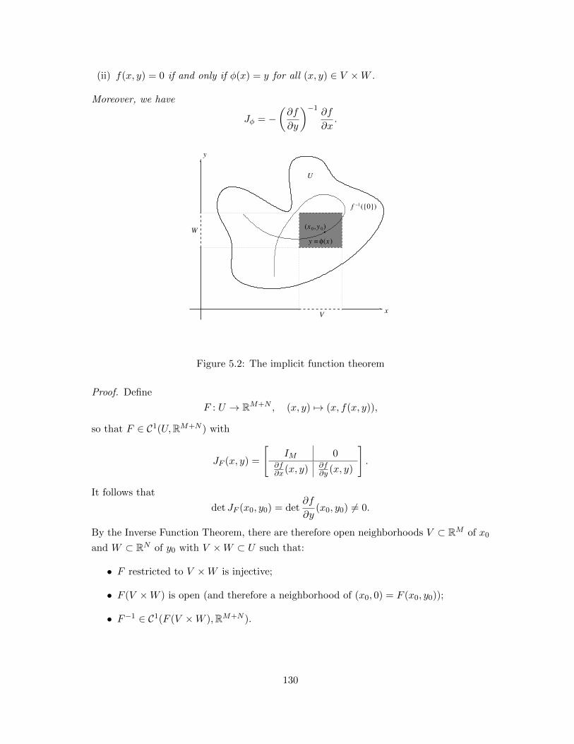
(ii) f(x, y) = 0 if and only if φ(x) = y for all (x, y) ∈ V ×W .
Moreover, we have
Jφ = −(∂f
∂y
)−1 ∂f
∂x.
=y φ(x)
x 0( ,y 0)
f −1({0})
x
y
W
V
U
Figure 5.2: The implicit function theorem
Proof. Define
F : U → RM+N , (x, y) 7→ (x, f(x, y)),
so that F ∈ C1(U,RM+N ) with
JF (x, y) =
[IM 0
∂f∂x (x, y) ∂f
∂y (x, y)
].
It follows that
det JF (x0, y0) = det∂f
∂y(x0, y0) 6= 0.
By the Inverse Function Theorem, there are therefore open neighborhoods V ⊂ RM of x0
and W ⊂ RN of y0 with V ×W ⊂ U such that:
• F restricted to V ×W is injective;
• F (V ×W ) is open (and therefore a neighborhood of (x0, 0) = F (x0, y0));
• F−1 ∈ C1(F (V ×W ),RM+N ).
130

Let
π : RM+N → RN , (x, y) 7→ y.
Then we have for (x, y) ∈ F (V ×W ) that
(x, y) = F (F−1(x, y)) = F (x, π(F−1(x, y))) = (x, f(x, π(F−1(x, y))))
and thus
y = f(x, π(F−1(x, y))).
Since {(x, 0) : x ∈ V } ⊂ F (V ×W ), we can define
φ : V → RN , x 7→ π(F−1(x, 0)).
It follows that φ ∈ C1(V,RN ) with φ(x0) = y0 and f(x, φ(x)) = 0 for all x ∈ V . If
(x, y) ∈ V ×W is such that f(x, y) = 0 = f(x, φ(x)), the injectivity of F—and hence of
f—yields y = φ(x). This also proves the uniqueness of φ.
Let
ψ : V → RM+N , x 7→ (x, φ(x)),
so that ψ ∈ C1(V,RM+N ) with
Jψ(x) =
[IM
Jφ(x)
]for x ∈ V . Since f ◦ ψ = 0, the chain rule yields for x ∈ V that
0 = Jf (ψ(x))Jψ(x)
=[
∂f∂x (ψ(x)) ∂f
∂y (ψ(x))] [ IM
Jφ(x)
]
=∂f
∂x(x, φ(x)) +
∂f
∂y(x, φ(x))Jφ(x)
and therefore
Jφ(x) = −(∂f
∂y(x, φ(x))
)−1 ∂f
∂x(x, φ(x)).
This completes the proof.
Example. The system
x2 + y2 − 2z2 = 0,
x2 + 2y2 + z2 = 4
of equations has the solutions x0 = 0, y0 =√
85 , and z0 =
√45 . Define
f : R3 → R2, (x, y, z) 7→ (x2 + y2 − 2z2, x2 + 2y2 + z2 − 4),
131

so that f(x0, y0, z0) = 0. Note that[∂f1∂y (x, y, z), ∂f1
∂z (x, y, z)∂f2∂y (x, y, z), ∂f2
∂z (x, y, z)
]=
[2y, −4z
4y, 2z
].
Hence,
det
[∂f1∂y (x, y, z), ∂f1
∂z (x, y, z)∂f2∂y (x, y, z), ∂f2
∂z (x, y, z)
]= 4yz + 16yz = 20yz 6= 0
whenever y 6= 0 6= z. By the Implicit Function Theorem, there is ε > 0 and a unique
φ ∈ C1((−ε, ε),R2) such that
φ1(0) =
√8
5, φ2(0) =
√4
5, and f(x, φ1(x), φ2(x)) = 0
for x ∈ (−ε, ε). Moroever, we have
Jφ(x) =
[dφ1dx (x)dφ2dx (x)
]= −
[2y, −4z
4y, 2z
]−1 [2x
2x
]
= − 1
20y2
[2z, 4z
−4y, 2y
][2x
2x
]=
[12xz20yz
−−4yx20yz
]=
[−3
5xy
15xz
]
and thus
φ′1(x) = −3
5
x
φ1(x)and φ′2(x) =
1
5
x
φ2(x)
for x ∈ (−ε, ε).
Exercises
1. Let
f : R2 → R, (x, y) 7→ x2 + y2.
Show that, there is ε > 0 and a C1-function φ : (−ε, ε)→ R with φ(0) = 1 such that
y = φ(x) solves the equation f(x, y) = 1 for all x ∈ R with |x| < ε. Show without
explicitly determining φ that
φ′(x) = − x
φ(x)(x ∈ (−ε, ε)).
2. Show that there are ε > 0, and u, v, w ∈ C1(Bε((1, 1)),R) such that u(1, 1) = 1,
v(1, 1) = 1, and w(1, 1) = −1, and
u(x, y)5 + x v(x, y)2 − y + w(x, y) = 0,
v(x, y)5 + y u(x, y)− x+ w(x, y) = 0,
132

and
w(x, y)4 + y5 − x4 = 1
for (x, y) ∈ Bε((1, 1)).
3. Let f0, . . . , fn−1 : R→ R be continuously differentiable, and let
p : R2 → R, (x, y) 7→ yn + fn−1(x)yn−1 + · · ·+ f1(x)y + f0(x).
Suppose that f0(0) = 0 and that f1(0) 6= 0. Show that there is ε > 0 and a unique
C1-function φ : (−ε, ε)→ R with φ(0) = 0 such that p(x, φ(x)) = 0 for all x ∈ (−ε, ε).
4. Let f ∈ C1(R2,R) be such that
f−1({0}) = {(x, y) ∈ R2 : (x− 1)2 + y2 = 1 or (x+ 1)2 + y2 = 1}.
(a) Sketch f−1({0}).
(b) Show that∂f
∂y(0, 0) =
∂f
∂x(0, 0) = 0.
5.3 Local Extrema under Constraints
Example. Let
f : B1[(0, 0)]→ R, (x, y) 7→ 4x2 − 3xy.
Since B1[(0, 0)] is compact, and f is continuous, there are (x1, y1), (x2, y2) ∈ B1[(0, 0)]
such that
f(x1, y1) = sup(x,y)∈B1[(0,0)]
f(x, y) and f(x2, y2) = inf(x,y)∈B1[(0,0)]
f(x, y).
The problem is to find (x1, y1) and (x2, y2). If (x1, y1) and (x2, y2) are in B1((0, 0)), then
f has local extrema at (x1, y1) and (x2, y2), and we know how to determine them.
Since∂f
∂x(x, y) = 8x− 3y and
∂f
∂y(x, y) = −3x,
the only stationary point for f in B1((0, 0)) is (0, 0). Furthermore, we have
∂2f
∂x2(x, y) = 8,
∂2f
∂y2(x, y) = 0, and
∂2f
∂x∂y(x, y) = −3,
so that
(Hess f)(x, y) =
[8 −3
−3 0
].
Since det(Hess f)(0, 0) = −9, it follows that f has a saddle at (0, 0).
Hence, (x1, y1) and (x2, y2) must lie in ∂B1[(0, 0)]. . .
133

There are, of course, ways to steer around the problem that occurs in this example.
For instance, we might parametrize the unit circle via
[0, 2π]→ R2, t 7→ (cos t, sin t)
and then determine the minimum and maximum—along with the values of t where they
are attained—of
[0, 2π]→ R, t 7→ 4(cos t)2 − 3(cos t)(sin t).
This would be an ad hoc solution that actually might lead to success, but is specific to the
particular problem. Instead, we develop a general approach to determine so-called local
extrema of functions under constraints.
We first make precise what this is supposed to mean:
Definition 5.3.1. Let ∅ 6= D ⊂ RN , and let f, φ : D → R. We say that f has a local
maximum [minimum] at x0 ∈ D under the constraint φ(x) = 0 if φ(x0) = 0 and if there
is a neighborhood U of x0 such that f(x) ≤ f(x0) [f(x) ≥ f(x0)] for all x ∈ U ∩D with
φ(x) = 0.
Theorem 5.3.2 (Lagrange Multiplier Theorem). Let ∅ 6= U ⊂ RN be open, let f, φ ∈C1(U,R), and let x0 ∈ U be such that f has a local extremum, i.e., a minimum or a
maximum, at x0 under the constraint φ(x) = 0 and such that ∇φ(x0) 6= 0. Then there is
λ ∈ R, a Lagrange multiplier, such that
∇f(x0) = λ∇φ(x0).
Proof. Without loss of generality suppose that ∂φ∂xN
(x0) 6= 0. By the Implicit Function
Theorem, there are an open neighborhood V ⊂ RN−1 of x0 := (x0,1, . . . , x0,N−1) and
ψ ∈ C1(V,R) such that
ψ(x0) = x0,N and φ(x, ψ(x)) = 0 for all x ∈ V .
It follows that
0 =∂φ
∂xj(x, ψ(x)) +
∂φ
∂xN(x, ψ(x))
∂ψ
∂xj(x)
for all j = 1, . . . , N − 1 and x ∈ V . In particular,
0 =∂φ
∂xj(x0) +
∂φ
∂xN(x0)
∂ψ
∂xj(x0) (5.2)
holds for all j = 1, . . . , N − 1.
The function
g : V → R, (x1, . . . , xN−1) 7→ f(x1, . . . , xN−1, ψ(x1, . . . , xN−1))
134

has a local extremum at x0, so that ∇g(x0) = 0 and thus
0 =∂g
∂xj(x0) =
∂f
∂xj(x0) +
∂f
∂xN(x0)
∂ψ
∂xj(x0) (5.3)
for j = 1, . . . , N − 1. Set
λ :=∂f
∂xN(x0)
(∂φ
∂xN(x0)
)−1
,
so that ∂f∂xN
(x0) = λ ∂φ∂xN
(x0) holds trivially. From (5.2) and (5.3), it also follows that
∂f
∂xj(x0) = − ∂f
∂xN(x0)
∂ψ
∂xj(x0) = −λ ∂φ
∂xN(x0)
∂ψ
∂xj(x0) = λ
∂φ
∂xj(x0)
holds as well for j = 1, . . . , N − 1. All in all, ∇f(x0) = λ∇φ(x0).
Example. Consider again
f : B1[(0, 0)]→ R, (x, y) 7→ 4x2 − 3xy.
Since f has no local extrema on B1((0, 0)), it must attain its minimum and maximum
on ∂B1[(0, 0)].
Let
φ : R2 → R, (x, y) 7→ x2 + y2 − 1,
so that
∂B1[(0, 0)] = {(x, y) ∈ R2 : φ(x, y) = 0}.
Hence, the mimimum and maximum of f on B1[(0, 0)] are local extrema under the con-
straint φ(x, y) = 0. Since ∇φ(x, y) = (2x, 2y) for x, y ∈ R, ∇φ never vanishes on
∂B1[(0, 0)].
Suppose that f has a local extremum at (x0, y0) under the constraint φ(x, y) = 0. By
the Lagrange Multiplier Theorem, there is thus λ ∈ R such that∇f(x0, y0) = λ∇φ(x0, y0),
i.e.,
8x0 − 3y0 = 2λx0,
−3x0 = 2λy0.
For notational simplicity, we write (x, y) instead of (x0, y0). Solve the equations:
8x− 3y = 2λx; (5.4)
−3x = 2λy; (5.5)
x2 + y2 = 1. (5.6)
From (5.5), it follows that x = −23λy. Plugging this expression into (5.4), we obtain
−16
3λy − 3y = −4
3λ2y. (5.7)
135

Case 1: y = 0. Then (5.5) implies x = 0, which contradicts (5.6). Hence, this case
cannot occur.
Case 2: y 6= 0. Dividing (5.7) by y3 yields
4λ2 − 16λ− 9 = 0
and thus
λ2 − 4λ− 9
4= 0.
Completing the square, we obtain (λ−2)2 = 254 and thus the solutions λ = 9
2 and λ = −12 .
Case 2.1: λ = −12 . Then (5.5) yields −3x = −y and thus y = 3x. Plugging into (5.6),
we get 10x2 = 1, so that x = ± 1√10
. Hence,(
1√10, 3√
10
)and
(− 1√
10,− 3√
10
)are possible
candidates for extrema to be attained at.
Case 2.2: λ = 92 . The (5.5) yields −3x = 9y and thus x = −3y. Plugging into (5.6),
we get 10y2 = 1, so that y = ± 1√10
. Hence,(
3√10,− 1√
10
)and
(− 3√
10, 1√
10
)are possible
candidates for extrema to be attained at.
Evaluating f at those points, we obtain:
f
(1√10,
3√10
)= −1
2;
f
(− 1√
10,− 3√
10
)= −1
2;
f
(3√10,− 1√
10
)=
9
2;
f
(− 3√
10,
1√10
)=
9
2.
All in all, f has on B1[(0, 0)] the maximum 92 , attained at
(3√10,− 1√
10
)and
(− 3√
10, 1√
10
),
and the minimum −12 , which is attained at
(1√10, 3√
10
)and
(− 1√
10,− 3√
10
).
Given a bounded, open set ∅ 6= U ⊂ RN an open set U ⊂ V ⊂ RN and a C1-function
f : V → R which is of class C1 on U , the following is a strategy to determine the minimum
and maximum (as well as those points in U where they are attained) of f on U :
• Determine all stationary points of f on U .
• If possible (with a reasonable amount of work), classify those stationary points and
evaluate f there in the case of a local extremum.
• If classifying the stationary points isn’t possible (or simply too much work), simply
evaluate f at all of its stationary points.
• Describe ∂U in terms of a constraint φ(x) = 0 for some φ ∈ C1(V,R) and check if
the Lagrange Multiplier Theorem is applicable.
136

• If so, determine all x ∈ V with φ(x) = 0 and ∇f(x) = λ∇φ(x) for some λ ∈ R, and
evaluate f at those points.
• Compare all the values of f you have obtain in the process and pick the largest and
the smallest one.
This is not a fail safe algorithm, but rather a strategy that may have to be modified
depending on the cirucmstances (or that may not even work at all. . . ).
Example. Let
K := {(x, y, z) ∈ R3 : x2 + 4y2 + z2 ≤ 9}
and
f : R3 → R, (x, y, z) 7→ xz + y(y − 1)
As K is compact and f is continuous, f attains both a minimum and a maximum on K.
We want to determine those values and the points in K where they are attained.
We first consider the interior of K. Since
∂f
∂x= z,
∂f
∂y= 2y − 1, and
∂f
∂z= x,
the only stationary point f has in the interior of K is(0, 1
2 , 0). Since
(Hess f)
(0,
1
2, 0
)=
0 0 1
0 2 0
1 0 0
,it is immediate that the Hessian can neither be positive nor negative definite (otherwise,
the upper left corner would not be zero). Since the Hessian clearly has rank three—and
thus is invertible—, it must be indefinite. Hence, f has a saddle at(0, 1
2 , 0).
To investigate the boundary of K, we apply the Lagrange multiplier theorem. Let
φ : R3 → R, (x, y, z) 7→ x2 + 4y2 + z2 − 9,
so that ∂K = {(x, y, z) ∈ R3 : φ(x, y, z) = 0}. We have to find solutions to the equations
z = 2λx, (5.8)
2y − 1 = 8λy, (5.9)
x = 2λz, (5.10)
and
x2 + 4y2 + z2 = 9. (5.11)
137

Plugging (5.10) into (5.8), we obtain z = 4λ2z.
Case 1: z 6= 0. It follows that λ2 = 14 , so that λ = ±1
2 .
Subcase 1.1: λ = 12 . Then (5.8) (or (5.10)) yields x = z. Moreover, (5.9) yields
2y − 1 = 4y and thus 2y = −1, i.e. y = −12 . Plugging into (5.11), we obtain 2x2 + 1 = 9,
i.e. x = ±2. Possible points on ∂K, where f could attain a minimum or a maximum are
therefore(2,−1
2 , 2)
and(−2,−1
2 ,−2). The values attained at those points are
f
(2,−1
2, 2
)= f
(−2,−1
2,−2
)=
19
4.
Subcase 1.2: λ = −12 . Then (5.8) yields x = −z. Moreover, (5.9) yields 2y − 1 = −4y
and thus 6y = 1, i.e. y = 16 . Plugging into (5.11), we obtain 2x2 + 1
9 = 9, i.e. x = ±2√
103 .
Candidates for points where f could attain a minimum or a maximum are therefore(2√
103 , 1
6 ,−2√
103
)and
(−2√
103 , 1
6 ,2√
103
). The values attained at those points are
f
(2√
10
3,1
6,−2√
10
3
)= f
(−2√
10
3,1
6,2√
10
3
)= −165
36.
Case 2: z = 0. Then (5.10) yields that x = 0 as well. From (5.11), we obtain that
4y2 = 9, i.e. y = ±32 . Therefore
(0, 3
2 , 0)
and(0,−3
2 , 0)
are also candidates for points
where an extremum could be attained at. The corresponding values attained by f at
those points are
f
(0,
3
2, 0
)=
3
4and f
(0,−3
2, 0
)=
15
4.
Thus, f attains on K the minimum −16536 at
(2√
103 , 1
6 ,−2√
103
)and
(−2√
103 , 1
6 ,2√
103
)and the maximum 19
4 at(2,−1
2 , 2)
and(−2,−1
2 ,−2).
Exercises
1. Determine the maximum and the minimum of
f : R2 → R, (x, y) 7→ (x− 1)2 + y2
on
K := {(x, y) ∈ R2 : x2 + y2 ≤ 4}.
as well as all points at which they are attained.
2. Determine the maximum and the minimum of
f : R2 → R, (x, y) 7→ x2 + y2 + xy
138

on
K := {(x, y) ∈ R2 : 2 ≤ x2 + y2 ≤ 8}.
Also, find all points in K, where the maximum and the minimum, respectively, are
attained.
3. Find the minimum and maximum of
f : R2 → R, (x, y) 7→ x2 − y2
on
K := {(x, y) : x2 + 2y2 ≤ 2}
and determine all points in K where the minimum and the maximum, respectively,
are attained.
4. Determine the maximum and minimum of
f : R3 → R, (x, y, z) 7→ xy + z2
on
B := {(x, y, z) ∈ R3 : x2 + y2 + z2 ≤ 2}
as well as all the points at which they are attained.
5. Of course, the definition of a local extremum under a constraint, can also be formu-
lated with respect to a vector-valued function φ. Prove the following generalization
of the Lagrange multiplier theorem from class:
Let ∅ 6= U ⊂ RN be open, let φ ∈ C1(U,RM ) with M < N , let f ∈ C1(U,R)
have a local extremum at x0 ∈ U under the constraint φ(x) = 0, and
suppose that Jφ(x0) has rank M . Then there are λ1, . . . , λM ∈ R such
that
(∇f)(x0) =M∑j=1
λj(∇φj)(x0).
5.4 Change of Variables
In this section, we shall actually prove the change of variables formula stated earlier:
Theorem 5.4.1 (Change of Variables). Let ∅ 6= U ⊂ RN be open, let ∅ 6= K ⊂ U be
compact with content, let φ ∈ C1(U,RN ), and suppose that there is a set Z ⊂ K with
content zero such that φ|K\Z is injective and det Jφ(x) 6= 0 for all x ∈ K \Z. Then φ(K)
has content and ∫φ(K)
f =
∫K
(f ◦ φ)| det Jφ|
holds for all continuous functions f : φ(U)→ RM .
139

The reason why we didn’t proof the theorem when we first encountered it were twofold:
first of all, there simply wasn’t enough time to both prove the theorem and cover ap-
plications, but secondly, the proof also requires some knowledge of local properties of
C1-functions, which wasn’t available to us then.
Before we delve into the proof, we give yet another example:
Example. Let
D := {(x, y) ∈ R2 : 1 ≤ x2 + y2 ≤ 4}
and determine ∫D
1
x2 + y2.
Use polar coordinates:
φ : R2 → R2, (r, θ) 7→ (r cos θ, r sin θ),
so that detJφ(r, θ) = r. Let K = [1, 2]× [0, 2π], so that φ(K) = D. It follows that∫D
1
x2 + y2=
∫K
r
r2=
∫K
1
r=
∫ 2
1
(∫ 2π
0
1
rdθ
)dr = 2π log 2.
To prove Theorem 5.4.1, we proceed through a series of steps.
Given a compact subset K of RN and a (sufficiently nice) C1-function φ on a neigh-
borhood of K, we first establish that φ(K) does indeed have content.
Lemma 5.4.2. Let ∅ 6= U ⊂ RN be open, let φ ∈ C1(U,RN ), and let K ⊂ U be compact
with content zero. Then φ(K) is compact with content zero.
Proof. Clearly, φ(K) is compact.
Choose an open set V ⊂ RN with K ⊂ V , and such that V ⊂ U is compact.
As φ is a C1-function, the map
U × RN → R, (x, ξ) 7→ ‖Jφ(x)ξ‖
is continuous; in particular, it is bounded on V ×B1[0], so that there is C > 0 such that
‖Jφ(x)ξ‖ ≤ C for all x ∈ V and all ξ ∈ RN with ‖ξ‖ ≤ 1. It follows that
‖Jφ(x)ξ‖ ≤ C‖ξ‖ (5.12)
for all xinV and all ξ ∈ RN .
Let ε > 0, and choose compact intervals I1, . . . , In ⊂ V with
K ⊂n⋃j=1
Ij andn∑j=1
µ(Ij) <ε
(2C√N)N
.
140

U
����������������������������������������������������������������������������������������������������������������������������������������������������������������������������������������������������������������������������������������������������������������������������������������������������������������������������������������������������������������������������������������������������������������������������������������������������������������������������������������������������������������������������������������������������������������������������������������������������������������������������������������������������������������������������������������������������
����������������������������������������������������������������������������������������������������������������������������������������������������������������������������������������������������������������������������������������������������������������������������������������������������������������������������������������������������������������������������������������������������������������������������������������������������������������������������������������������������������������������������������������������������������������������������������������������������������������������������������������������������������������������������������������������������
������������������������������������������������������������������������������������������������������������������������������������������������������������������������������������������������������������������������������������������������������������������������������������������������������������������������������������������������������
������������������������������������������������������������������������������������������������������������������������������������������������������������������������������������������������������������������������������������������������������������������������������������������������������������������������������������������������������
K
V
Figure 5.3: K, U , V , and I1, . . . , In
Without loss of generality, suppose that each Ij is a cube, i.e.,
Ij = [xj,1 − rj , xj,1 + rj ]× · · · × [xj,N − rj , xj,N + rj ]
with (xj,1, . . . , xj,N ) ∈ RN and rj > 0: this can be done by first making sure that each Ij
is of the form
Ij = [a1, b1]× · · · × [aN , bN ]
with a1, b1, . . . , an, bN ∈ Q, so that the ratios between the lengths of the different sides of
Ij are rational, and then splitting it into sufficiently many cubes.
Figure 5.4: Splitting a 2-dimensional interval into cubes
(You’re asked to work out the details in Exercise 1 below.)
141

Let j ∈ {1, . . . , n}, and let x, y ∈ Ij . Then we have
|φk(x)− φk(y)| ≤ ‖φ(x)− φ(y)‖
=
∥∥∥∥∫ 1
0Jφ(x+ t(y − x))(y − x) dt
∥∥∥∥≤∫ 1
0‖Jφ(x+ t(y − x))(y − x)‖ dt
≤∫ 1
0C‖x− y‖ dt, by (5.12),
= C‖x− y‖
= C
√√√√ N∑ν=1
(xν − yν)2
≤ C
√√√√ N∑ν=1
(2rj)2
= C√N 2rj
= C√N µ(Ij)
1N .
for k = 1, . . . , N .
Fix x0 ∈ Ij , and Rj := C√N µ(Ij)
1N , and define
Jj := [φ1(x0)−Rj , φ1(x0) +Rj ]× · · · × [φN (x0)−Rj , φN (x0) +Rj ].
It follows that φ(Ij) ⊂ Jj and that
µ(Jj) = (2Rj)N = (2C
√N)Nµ(Ij)
All in all we obtain, that
φ(K) ⊂n⋃j=1
Jj andn∑j=1
µ(Jj) = (2C√N)N
n∑j=1
µ(Ij) < ε.
Hence, φ(K) has content zero.
Lemma 5.4.3. Let ∅ 6= U ⊂ RN be open, let φ ∈ C1(U,RN ) be such that det Jφ(x) 6= 0
for all x ∈ U , and let ∅ 6= K ⊂ U be compact. Then
{x ∈ K : φ(x) ∈ ∂φ(K)} ⊂ ∂K
holds. In particular, ∂φ(K) ⊂ φ(∂K) holds.
Proof. Let x ∈ K be such that φ(x) ∈ ∂φ(K), and let V ⊂ U be a neighborhood x, which
we can suppose to be open. By Lemma 5.1.5, φ(V ) is a neighborhood of φ(x), and since
142

φ(x) ∈ ∂φ(K), it follows that φ(V ) ∩ (RN \ φ(K)) 6= ∅. Assume that V ⊂ K. Then
φ(V ) ⊂ φ(K) holds, which contradicts φ(V ) ∩ (RN \ φ(K)) 6= ∅. Consequently, we have
V ∩ (RN \K) 6= ∅. Since trivially V ∩K 6= ∅, we conclude that x ∈ ∂K.
Since φ(K) is compact and therefore closed, we have ∂φ(K) ⊂ φ(K) and thus ∂φ(K) ⊂φ(∂K).
Proposition 5.4.4. Let ∅ 6= U ⊂ RN be open, let φ ∈ C1(U,RN ) be such that det Jφ(x) 6=0 for all x ∈ U , and let ∅ 6= K ⊂ U be compact with content. Then φ(K) is compact with
content.
Proof. Since K has content, ∂K has content zero. From Lemma 5.4.2, we conclude that
µ(φ(∂K)) = 0. Since ∂φ(K) ⊂ φ(∂K) by Lemma 5.4.3, it follows that µ(∂φ(K)) = 0. By
Theorem 4.2.11, this means that φ(K) has content.
Next, we investigate how applying a C1-function to a set with content affects that
content.
Lemma 5.4.5. Let D ⊂ RN have content. Then
µ(D) = inf
n∑j=1
µ(Ij) (5.13)
holds, where the infimum is taken over all n ∈ N and all compact intervals I1, . . . , In ⊂ RN
such that D ⊂ I1 ∪ · · · ∪ In.
Proof. See Exercise 2 below.
Proposition 5.4.6. Let ∅ 6= K ⊂ RN be compact with content, and let T : RN → RN be
linear. Then T (K) has content such that
µ(T (K)) = |detT |µ(K).
Proof. We first prove three separate cases of the claim:
Case 1:
T (x1, . . . , xN ) = (x1, . . . , λxj , . . . xN )
with λ ∈ R for x1, . . . , xN ∈ R.
Suppose first that K is an interval, say K = [a1, b1]× · · · × [aN , bN ], so that
T (K) = [a1, b1]× · · · × [λaj , λbj ]× · · · × [aN , bN ]
if λ ≥ 0 and
T (K) = [a1, b1]× · · · × [λbj , λaj ]× · · · × [aN , bN ]
if λ < 0. Since detT = λ, this settles the claim in this particular case.
143

Suppose that K is now arbitrary and λ 6= 0. Then T is invertible, so that T (K)
has content by Proposition 5.4.4. For any closed intervals I1, . . . , In ⊂ RN with K ⊂I1 ∪ . . . ∪ In, we then obtain
µ(T (K)) ≤n∑j=1
µ(T (Ij)) = |detT |n∑j=1
µ(Ij)
and thus µ(T (K)) ≤ |detT |µ(K) by Lemma 5.4.5. Since T−1 is of the same form, we get
also get µ(K) = µ(T−1(T (K))) ≤ |detT |−1µ(T (K)) and thus µ(T (K)) ≥ |detT |µ(K).
For arbitrary K and λ = 0, let I ⊂ RN be a compact interval with K ⊂ I. Then T (I)
has content zero, and so has T (K) ⊂ T (I).
Case 2:
T (x1, . . . , xj , . . . , xk, . . . , xN ) = (x1, . . . , xk, . . . , xj , . . . , xN )
with j < k for x1, . . . , xN ∈ R. Again, T is invertible, so that T (K) has content by
Proposition 5.4.4. Since detT = −1, the claim is trivially true if K is an interval and for
general K by Lemma 5.4.5 in a way similar to Case 1.
Case 3:
T (x1, . . . , xj , . . . , xk, . . . , xN ) = (x1, . . . , xj , . . . , xk + xj , . . . , xN )
with j < k for x1, . . . , xN ∈ R. It is clear that then T is invertible, so that T (K) has
content by Proposition 5.4.4. Again, suppose first that K is a compact interval. As only
the two coordinates j and k are concerned, it follows from a straightforward application
of Fubini’s Theorem, that we can limit ourselves to the case where j = 1 and k = N = 2.
Let K = [a, b]× [c, d], so that
T (K) = {(x, x+ y) ∈ R2 : x ∈ [a, b], y ∈ [c, d]}
= {(x, y) ∈ R2 : x ∈ [a, b], c+ x ≤ y ≤ d+ x}.
Applying Fubini’s Theorem again, we obtain
µ(T (K)) =
∫ b
a
∫ d+x
c+x1 dy dx
=
∫ b
a(d− c) dx
= (b− a)(d− c)
= µ(K).
Since detT = 1, this settles the claim in this case.
Now, let K be arbitrary. Invoking Lemma 5.4.5 as in Case 1, we obtain µ(T (K)) ≤µ(K). Obtaining the reversed inequality is a little bit harder than in Cases 1 and 2 because
144

T−1 is not of the form covered by Case 3 (in fact, it isn’t covered by any of Cases 1, 2,
3). Let S : RN → RN be defined by
S(x1, . . . , xj , . . . , xN ) = (x1, . . . ,−xj , . . . , xN ).
It follows that T−1 = S ◦ T ◦ S, so that—in view of Case 1—we get
µ(K) = µ(T−1(T (K))
= µ(S(T (S(T (K))))) = µ(T (S(T (K)))) ≤ µ(S(T (K))) = µ(T (K)).
All in all, µ(T (K)) = µ(K) holds.
Suppose now that T is arbitrary. Then there are linear maps T1, . . . , Tn : RN → RN
such that T = T1 ◦ · · · ◦Tn, and each Tj is of one of the forms discussed in Cases 1, 2, and
3. We therefore obtain eventually
µ(T (K)) = µ(T1(· · ·Tn(K) · · · ))
= |detT1|µ(T2(· · ·Tn(K) · · · )) = · · · = |detT1| · · · |detTn|µ(K) = |detT |µ(K).
This completes the proof.
Next, we move from linear maps to C1-maps:
Lemma 5.4.7. Let U ⊂ RN be open, let r > 0 be such that K := [−r, r]N ⊂ U , and
let φ ∈ C1(U,RN ) be such that det Jφ(x) 6= 0 for all x ∈ K. Furthermore, suppose that
α ∈(
0, 1√N
)is such that ‖φ(x)− x‖ ≤ α‖x‖ for x ∈ K. Then
(1− α√N)N ≤ µ(φ(K))
µ(K)≤ (1 + α
√N)N
holds.
Proof. Let x ∈ K. Then
‖φ(x)− x‖ ≤ α‖x‖ ≤ α√N r
holds and, consequently,
|φj(x)| ≤ |xj |+ ‖φ(x)− x‖ ≤ (1 + α√N)r
for j = 1, . . . , N . This means that
φ(K) ⊂ [−(1 + α√N)r, (1 + α
√N)r]N . (5.14)
Let x = (x1, . . . , xN ) ∈ ∂K, so that |xj | = r for some j ∈ {1, . . . , N}. Consequently,
r = |xj | ≤ ‖x‖ ≤√N r
145
holds and thus
|φj(x)| ≥ |xj | − ‖x− φ(x)‖ ≥ (1− α√N)r.
Since ∂φ(K) ⊂ φ(∂K) by Lemma 5.4.3, this means that
∂φ(K) ⊂ φ(∂K) ⊂ RN \ (−(1− α√N)r, (1− α
√N)r)N
and thus
(−(1− α√N)r, (1− α
√N)r)N ⊂ RN \ ∂φ(K).
Let U := int φ(K) and V := int (RN \ φ(K)). Then U and V are open, non-empty,
and satisfy
U ∪ V = RN \ ∂φ(K).
Since (−(1 − α√N)r, (1 − α
√N)r)N is connected, this means that it is contained either
in U or in V . Since
‖φ(0)‖ = ‖φ(0)− 0‖ ≤ α‖0‖ = 0,
it follows that 0 ∈ (−(1− α√N)r, (1− α
√N)r)N ∩ U and thus
(−(1− α√N)r, (1− α
√N)r)N ⊂ U ⊂ φ(K). (5.15)
From (5.14) and (5.15), we conclude that
(1− α√N)N (2r)N ≤ µ(φ(K)) ≤ (1 + α
√N)N (2r)N .
Division by µ(K) = (2r)N yields the claim.
For x = (x1, . . . , xN ) ∈ RN and r > 0, we denote by
K[x, r] := [x1 − r, x1 + r]× · · · × [xN − r, xN + r]
the cube with center x and side length 2r.
Proposition 5.4.8. Let ∅ 6= U ⊂ RN be open, and let φ ∈ C1(U,RN ) be such that
det Jφ(x) 6= 0 for all x ∈ U . Then, for each compact set ∅ 6= K ⊂ U and for each
ε ∈ (0, 1), there is rε > 0 such that K[x, r] ⊂ U and
|det Jφ(x)|(1− ε)N ≤ µ(φ(K[x, r]))
µ(K[x, r])≤ |det Jφ(x)|(1 + ε)N
for all x ∈ K and for all r ∈ (0, rε).
Proof. Let C > 0 be such that
‖Jφ(x)−1ξ‖ ≤ C‖ξ‖
146

for all x ∈ K and ξ ∈ RN , and choose rε > 0 such that K[x+ ξ, rε] ⊂ U and
‖φ(x+ ξ)− φ(x)− Jφ(x)ξ‖ ≤ ε
C√N‖ξ‖
for all x ∈ K and ξ ∈ K[0, rε]. Fix x ∈ K, and define
ψ(ξ) := Jφ(x)−1(φ(x+ ξ)− φ(x)).
For r ∈ (0, rε), we thus have
‖ψ(ξ)−ξ‖ = ‖Jφ(x)−1(φ(x+ξ)−φ(x)−Jφ(x)ξ)‖ ≤ C‖φ(x+ξ)−φ(x)−Jφ(x)ξ‖ ≤ ε√N‖ξ‖
for ξ ∈ K[0, r]. From Lemma 5.4.7 (with α = ε√N
), we conclude that
(1− ε)N ≤ µ(ψ(K[0, r]))
µ(K[0, r])≤ (1 + ε)N . (5.16)
Since
ψ(K[0, r]) = Jφ(x)−1φ(K[x, r])− Jφ(x)−1φ(x),
Proposition 5.4.6 yields that
µ(ψ(K[0, r])) = µ(Jφ(x)−1φ(K[x, r])) = |det Jφ(x)−1|µ(φ(K[x, r])).
Since µ(K[0, r]) = µ(K[x, r]), multiplying (5.16) with |det Jφ(x)| we obtain
|det Jφ(x)|(1− ε)N ≤ µ(φ(K[x, r]))
µ(K[x, r])≤ |det Jφ(x)|(1 + ε)N ,
as claimed.
We can now prove:
Theorem 5.4.9. Let ∅ 6= U ⊂ RN be open, let ∅ 6= K ⊂ U be compact with content, let
φ ∈ C1(U,RN ) be injective on K and such that det Jφ(x) 6= 0 for all x ∈ K. Then φ(K)
has content and ∫φ(K)
f =
∫K
(f ◦ φ)| det Jφ| (5.17)
holds for all continuous functions f : φ(U)→ RM .
Proof. Let f : φ(U)→ RM be continuous. By Proposition 5.4.4, φ(K) has content. Hence,
both integrals in (5.17) exist, and we are left with showing that they are equal.
Suppose without loss of generality that M = 1. Since
f =1
2(f + |f |)︸ ︷︷ ︸≥0
− 1
2(|f | − f)︸ ︷︷ ︸≥0
,
147

we can also suppose that f ≥ 0.
For each x ∈ K, choose Ux ⊂ U open with with x ∈ Ux and det Jφ(y) 6= 0 for all
y ∈ Ux. Since {Ux : x ∈ K} is an open cover of K, there are x1, . . . , xl ∈ K with
K ⊂ Ux1 ∪ · · · ∪ Uxl .
Replacing U by Ux1 ∪ · · · ∪ Uxl , we can thus suppose that det Jφ(x) 6= 0 for all x ∈ U .
Let ε ∈ (0, 1), and choose compact intervals I1, . . . , In ⊂ U with the following proper-
ties:
(a) for j 6= k, the intervals Ij and Ik have only boundary points in common, and we
have K ⊂⋃nj=1 Ij ⊂ U ;
(b) if m ≤ n is such that Ij ∩∂K 6= ∅ if and only if j ∈ {1, . . . ,m}, then∑m
j=1 µ(Ij) < ε
holds (this is possible because µ(∂K) = 0);
(c’) for any choice of ξj , ηj ∈ Ij for j = 1, . . . , n we have∣∣∣∣∣∣∫K
(f ◦ φ)| det Jφ| −n∑j=1
(f ◦ φ)(ξj)|det Jφ(ηj)|µ(Ij)
∣∣∣∣∣∣ < ε
(see Exercise 3 below). Arguing as in the proof of Lemma 5.4.2, we can suppose that
I1, . . . , In are actually cubes with centers x1, . . . , xn, respectively. From (c’), we then
obtain
(c) ∣∣∣∣∣∣∫K
(f ◦ φ)| det Jφ| −n∑j=1
(f ◦ φ)(ξj)|det Jφ(xj)|µ(Ij)
∣∣∣∣∣∣ < ε.
for any choice of ξj ∈ Ij for j = 1, . . . , n (see again Exercise 3 below).
Making our cubes even smaller, we can also suppose that
(d)
| det Jφ(xj)|(1− ε)N ≤µ(φ(Ij))
µ(Ij)≤ |det Jφ(xj)|(1 + ε)N
for j = 1, . . . , n.
Let V ⊂ U be open and bounded such that
n⋃j=1
Ij ⊂ V ⊂ V ⊂ U,
148
and let C := sup{|det Jφ(x)| : x ∈ V }. Together, (b) and (d) yield that
m∑j=1
µ(φ(Ij)) ≤ 2NCε.
Let j ∈ {m+ 1, . . . , n}, so that Ij ∩ ∂K = ∅, but Ij ∩K 6= ∅. As in the proof of Lemma
5.4.7, the connectedness of Ij yields that Ij ⊂ K. Note that, thanks to the injectivity of
φ on K, we have
φ(K) \n⋃
j=m+1
φ(Ij) = φ
K \ n⋃j=m+1
Ij
.
Let C := sup{|f(φ(x))| : x ∈ V }, and note that∣∣∣∣∣∣∫φ(K)
f −n∑j=1
∫φ(Ij)
f
∣∣∣∣∣∣ ≤∣∣∣∣∣∣∫φ(K)
f −n∑
j=m+1
∫φ(Ij)
f
∣∣∣∣∣∣+
∣∣∣∣∣∣m∑j=1
∫φ(Ij)
f
∣∣∣∣∣∣≤∫φ(K\
⋃nj=m+1 Ij)
f + 2NCCε
≤∫φ(
⋃mj=1 Ij)
f + 2NCCε
≤ 2N+1CCε. (5.18)
Let j ∈ {1, . . . , n}. Since the set φ(Ij) is connected, there is yj ∈ φ(Ij) such that∫φ(Ij)
f = f(yj)µ(φ(Ij)); choose ξj ∈ Ij such that yj = φ(ξj). It follows that
n∑j=1
∫φ(Ij)
f =n∑j=1
f(yj)µ(φ(Ij)) =n∑j=1
f(φ(ξj))µ(φ(Ij)). (5.19)
Since f ≥ 0, we obtain
n∑j=1
f(φ(ξj))|det Jφ(xj)|µ(Ij)(1− ε)N (5.20)
≤n∑j=1
f(φ(ξj))µ(φ(Ij)), by (d),
=
n∑j=1
∫φ(Ij)
f, by (5.19), (5.21)
≤n∑j=1
f(φ(ξj))| det Jφ(xj)|µ(Ij)(1 + ε)N , again by (5.19) and (d). (5.22)
As ε → 0, both (5.20) and (5.22) converge to the right hand side of (5.17) by (c),
whereas (5.21) converges to the left hand side of (5.17) by (5.18).
149

Even though Theorem 5.4.1 almost looks like the Change of Variables Theorem, it is
still not general enough to cover polar, spherical, or cylindrical coordinates.
Proof of Theorem 5.4.1. We leave showing that φ(K) has content as an exercise (see be-
low).
Let ε > 0, and let C > 0 be such that
C ≥ sup{|f(φ(x)) detJφ(x)|, |f(φ(x))| : x ∈ K}.
Choose compact intervals I1, . . . , In ⊂ U and J1, . . . , Jn ⊂ RN such that φ(Ij) ⊂ Jj for
j = 1, . . . , N ,
Z ⊂n⋃j=1
int Ij ,
n∑j=1
µ(Ij) <ε
2C, and
n∑j=1
µ(Jj) <ε
2C.
Let K0 := K \⋃nj=1 int Ij . Then K0 is compact, φ|K0 is injective and det Jφ(x) 6= 0 for
x ∈ K0. From Theorem 5.4.9, we conclude that∫φ(K0)
f =
∫K0
(f ◦ φ)|det Jφ|.
From the choice of the intervals Ij , it follows that∣∣∣∣∫K
(f ◦ φ)|det Jφ| −∫K0
(f ◦ φ)| det Jφ|∣∣∣∣ < ε
2,
and since φ(K) \ φ(K0) ⊂ J1 ∪ · · · ∪ Jn, the choice of J1, . . . , Jn yields∣∣∣∣∣∫φ(K)
f −∫φ(K0)
f
∣∣∣∣∣ < ε
2.
We thus conclude that ∣∣∣∣∣∫φ(K)
f −∫K
(f ◦ φ)| det Jφ|
∣∣∣∣∣ < ε.
Since ε > 0 is arbitrary, this completes the proof.
Example. For R > 0, let D ⊂ R3 be the upper hemisphere of the ball centered at 0 with
radius R intersected with the cylinder standing on the xy-plane, whose hull interesects
that plane in the circle given by the equation
x2 −Rx+ y2 = 0. (5.23)
What is the volume of D?
150

First note that
x2 −Rx+ y2 = 0 ⇐⇒ x2 − 2R
2x+
R2
4+ y2 =
R2
4
⇐⇒(x− R
2
)2
+ y2 =R2
4.
Hence, (5.23) describes a circle centered at(R2 , 0)
with radius R2 . It follows that
D =
{(x, y, z) ∈ R3 : x2 + y2 + z2 ≤ R2, z ≥ 0,
(x− R
2
)2
+ y2 ≤ R2
4
}= {(x, y, z) ∈ R3 : x2 + y2 + z2 ≤ R2, z ≥ 0, x2 + y2 ≤ Rx}.
R2
x
y
z
R
Figure 5.5: Intersection of a ball with a cylinder
Use cylindrical coordinates, i.e.,
φ : R3 → R3, (r, θ, z) 7→ (r cos θ, r sin θ, z).
Since
x2 + y2 ≤ Rx ⇐⇒ r2 = r2(cos θ)2 + r2(sin θ)2 ≤ Rr cos θ
⇐⇒ r ≤ R cos θ,
it follows that D = φ(K) with
K :={(r, θ, z) ∈ [0,∞)× [−π, π]× R : θ ∈
[−π
2,π
2
], r ∈ [0, R cos θ], z ∈
[0,√R2 − r2
]}.
151

The Change of Variables Formula then yields
µ(D) =
∫D
1
=
∫K
(1 ◦ φ)| det Jφ|
=
∫Kr
=
∫ π2
−π2
(∫ R cos θ
0
(∫ √R2−r2
0r dz
)dr
)dθ
=
∫ π2
−π2
(∫ R cos θ
0r√R2 − r2 dr
)dθ
= −1
2
∫ π2
−π2
(∫ R cos θ
0(−2r)
√R2 − r2 dr
)dθ
= −1
2
∫ π2
−π2
(∫ R2−R2(cos θ)2
R2
√u du
)dθ
=1
2
∫ π2
−π2
(∫ R2
R2(sin θ)2
√u du
)dθ
=1
2
∫ π2
−π2
2
3u
32
∣∣∣∣u=R2
u=R2(sin θ)2dθ
=1
3
∫ π2
−π2
(R3 −R3| sin θ|3) dθ
=R3
3π − R3
3
∫ π2
−π2
| sin θ|3 dθ.
We perform an auxiliary calculation. First note that∫ π2
−π2
| sin θ|3 dθ = 2
∫ π2
0(sin θ)3 dθ.
152

As ∫ π2
0(sin θ)3 dθ =
∫ π2
0(sin θ)(sin θ)2 dθ
=
∫ π2
0(sin θ)(1− (cos θ)2) dθ
=
∫ π2
0sin θ dθ +
∫ π2
0(− sin θ)(cos θ)2 dθ
= 1 +
∫ 0
1u2 du
= 1−∫ 1
0u2 du
=2
3,
it follows that ∫ π2
−π2
| sin θ|3 dθ =4
3.
All in all, we obtain that
µ(D) =R3
3
(π − 4
3
).
Exercises
1. An N -dimensional cube is a subset C of RN such that
C = [x1 − r, x1 + r]× · · · × [xN − r, xN + r]
with x1, . . . , xN ∈ R and r > 0.
Let ∅ 6= U ⊂ RN be open and let Z ⊂ U be compact with content zero. Show that,
for each ε > 0, there are cubes C1, . . . , Cn ⊂ U with
Z ⊂ C1 ∪ · · · ∪ Cn and
n∑j=1
µ(Cj) < ε.
2. Let D ⊂ RN have content. Show that
µ(D) = infn∑j=1
µ(Ij)
holds, where the infimum on the right hand side is taken over all n ∈ N and all
compact intervals I1, . . . , In ⊂ RN such that D ⊂ I1 ∪ · · · ∪ In.
153

3. Let I ⊂ RN be a compact interval, let f, g : I → R be continuous, and let ε > 0.
Show that there is a partition Pε of I such that, for each refinement P of Pε, we
have ∣∣∣∣∣∫Ifg −
∑ν
f(xν)g(yν)µ(Iν)
∣∣∣∣∣ < ε,
where (Iν)ν is the subdivision of I corresponding to P and xν , yν ∈ Iν are arbitrary.
4. Show that:
(a) if D ⊂ RN has content, then so has D such that µ(D) = µ(D);
(b) if ∅ 6= U ⊂ RN is open, Z is a set of content zero with Z ⊂ U , and φ : U → RN
is a C1-function, then φ(Z) has content zero.
5. Let ∅ 6= U ⊂ RN be open, let K ⊂ U be compact with content, let φ ∈ C1(U,RN ),
and suppose that there is Z ⊂ K with content zero such that det Jφ(x) 6= 0 for all
x ∈ K \Z. Show that φ(K) has content. (Hint : Show that ∂φ(K) ⊂ φ(Z)∪φ(∂K).)
6. Let C be the cylinder standing perpendicularly on the xy-plane such that its inter-
section with that plane is the closed unit disc, and let P be the prism (extending
from −∞ to∞ along the y-axis) standing perpendicularly on the xz-plane such that
its intersection with that plane is the diamond given by |x|+ |z| ≤ 1. Compute the
content of C ∩ P .
7. We may identify C with R2. For 0 < ρ < R, let
AR,ρ := {z ∈ C : ρ ≤ |z| ≤ R}.
Calculate∫AR,ρ
1z .
8. Let ∅ 6= K ⊂ R3 be a compact body with content, and let µ : K → R be a continuous
density. The Newton potential generated by K at x0 ∈ R3 \ K is given (up to a
factor) by
u(x0) :=
∫K
µ(x)
‖x0 − x‖dx.
Suppose that K = BR[(0, 0, 0)] with R > 0, and that µ is rotation symmetric, i.e.,
there is a continuous function µ : [0, R]→ R such µ(x) = µ(‖x‖) for all x ∈ K. Show
that
u(x0) =1
‖x0‖
∫Kµ.
for all x0 ∈ R3 \K. (Hint : First, argue that we can suppose that x0 = (0, 0, ‖x0‖)without loss of generality; then use spherical coordinates.)
9. Show that a slice of pizza of radius r > 0 and with angle α has the area 12r
2α.
154

Chapter 6
Curve and Surface Integrals and
the Integral Theorems by Green,
Gauß, and Stokes
6.1 Curves in RN
What is the circumference of a circle of radius r > 0? Of course, we “know” the answer:
2πr. But how can this be proven? More generally, what is the length of a curve in the
plane, in space, or in general N -dimensional Euclidean space?
We first need a rigorous definition of a curve:
Definition 6.1.1. A curve in RN is a continuous map γ : [a, b] → RN . The set {γ} :=
γ([a, b]) is called the trace or line element of γ.
Examples. 1. For r > 0, let
γ : [0, 2π]→ R2, t 7→ (r cos t, r sin t).
Then {γ} is a circle centered at (0, 0) with radius r.
2. Let c, v ∈ RN with v 6= 0, and let
γ : [a, b]→ RN , t 7→ c+ tv.
Then {γ} is the line segment from c + av to c + bv. Slightly abusing terminology,
we will also call γ a line segment.
3. Let γ : [a, b] → RN be a curve, and suppose that there is a partition a = t0 < t1 <
· · · < tn = b such that γ|[tj−1,tj ] is a line segment for j = 1, . . . , n. Then γ is called
a polygonal path: one can think of it as a concatenation of line segments.
155

4. For r > 0 and s 6= 0, let
γ : [0, 6π]→ R3, t 7→ (r cos t, r sin t, st).
Then {γ} is a helix:
y
x
z
r
Figure 6.1: Helix
If γ : [a, b]→ RN is a line segment, it makes sense to define its length as ‖γ(b)−γ(a)‖.It is equally intuitive how to define the length of a polygonal path: sum up the lengths of
all the line segments it is made up of.
For more general curves, one tries to successively approximate them with polygonal
paths:
x
y
γ
Figure 6.2: Successive approximation of a curve with polygonal paths
156

This motivates the following definition:
Definition 6.1.2. A curve γ : [a, b]→ RN is called rectifiable ifn∑j=1
‖γ(tj−1)− γ(tj)‖ : n ∈ N, a = t0 < t1 < · · · < tn = b
(6.1)
is bounded. The supremum of (6.1) is called the length of γ.
Even though this definition for the length of a curve is intuitive, it does not provide
any effective means to calculate the length of a curve (except for polygonal paths).
Lemma 6.1.3. Let γ : [a, b] → RN be a C1-curve. Then, for each ε > 0, there is δ > 0
such that ∥∥∥∥γ(t)− γ(s)
t− s− γ′(t)
∥∥∥∥ < ε
for all s, t ∈ [a, b] such that 0 < |s− t| < δ.
Proof. Let ε > 0, and suppose first that N = 1. Since γ′ is uniformly continuous on [a, b],
there is δ > 0 such that
|γ′(s)− γ′(t)| < ε
for s, t ∈ [a, b] with |s − t| < δ. Fix s, t ∈ [a, b] with 0 < |s − t| < δ. By the mean value
theorem, there is ξ between s and t such that
γ(t)− γ(s)
t− s= γ′(ξ).
It follows that ∣∣∣∣γ(t)− γ(s)
t− s− γ′(t)
∣∣∣∣ = |γ′(ξ)− γ′(t)| < ε
Suppose now that N is arbitrary. By the case N = 1, there are δ1, . . . , δN > 0 such
that, for j = 1, . . . , N , we have∣∣∣∣γj(t)− γj(s)t− s− γ′j(t)
∣∣∣∣ < ε√N
for all s, t ∈ [a, b] such that 0 < |s− t| < δj . Since∥∥∥∥γ(t)− γ(s)
t− s− γ′(t)
∥∥∥∥ ≤ √N maxj=1,...,N
∣∣∣∣γj(t)− γj(s)t− s− γ′j(t)
∣∣∣∣for s, t ∈ [a, b], s 6= t, this yields the claim with δ := minj=1,...,N δj .
Theorem 6.1.4. Let γ : [a, b] → RN be a C1-curve. Then γ is rectifiable, and its length
is calculated as ∫ b
a‖γ′(t)‖ dt.
157

Proof. Let ε > 0.
There is δ1 > 0 such that∣∣∣∣∣∣∫ b
a‖γ′(t)‖ dt−
n∑j=1
‖γ′(ξj)‖(tj − tj−1)
∣∣∣∣∣∣ < ε
2
for each partition a = t0 < t1 < · · · < tn = b and ξj ∈ [tj−1, tj ] such that tj − tj−1 < δ1
for j = 1, . . . , n. Moreover, by Lemma 6.1.3, there is δ2 > 0 such that∥∥∥∥γ(t)− γ(s)
t− s− γ′(t)
∥∥∥∥ < ε
2(b− a)
for s, t ∈ [a, b] such that 0 < |s− t| < δ2.
Let δ := min{δ1, δ2}, and let a = t0 < t1 < · · · < tn = b such that maxj=1,...,n(tj −tj−1) < δ. First, note that
|‖γ(tj)− γ(tj−1)‖ − ‖γ′(tj)‖(tj − tj−1)| < ε
2
tj − tj−1
b− afor j = 1, . . . , n. It follows that∣∣∣∣∣∣
n∑j=1
‖γ(tj)− γ(tj−1)‖ −∫ b
a‖γ′(t)‖ dt
∣∣∣∣∣∣≤
∣∣∣∣∣∣n∑j=1
‖γ(tj)− γ(tj−1)‖ −n∑j=1
‖γ′(tj)‖(tj − tj−1)
∣∣∣∣∣∣+
∣∣∣∣∣∣n∑j=1
‖γ′(tj)‖(tj − tj−1)−∫ b
a‖γ′(t)‖ dt
∣∣∣∣∣∣<
n∑j=1
|‖γ(tj)− γ(tj−1)‖ − ‖γ′(tj)‖(tj − tj−1)|︸ ︷︷ ︸< ε
2
tj−tj−1b−a
+ε
2
< ε.
This yields the claim.
Let now a = s0 < s1 < · · · < sm = b be any partition, and choose a partition a = t0 <
t1 < · · · < tn = b such that maxj=1,...,N (tj − tj−1) < δ and {s0, . . . , sm} ⊂ {t0, . . . , tn}. By
the foregoing, we then obtain that
m∑j=1
‖γ(sj−1)− γ(sj)‖ ≤n∑j=1
‖γ(tj−1)− γ(tj)‖ <∫ b
a‖γ′(t)‖ dt+ ε
and, since ε > 0 is arbitrary,
m∑j=1
‖γ(sj−1)− γ(sj)‖ ≤∫ b
a‖γ′(t)‖ dt.
158
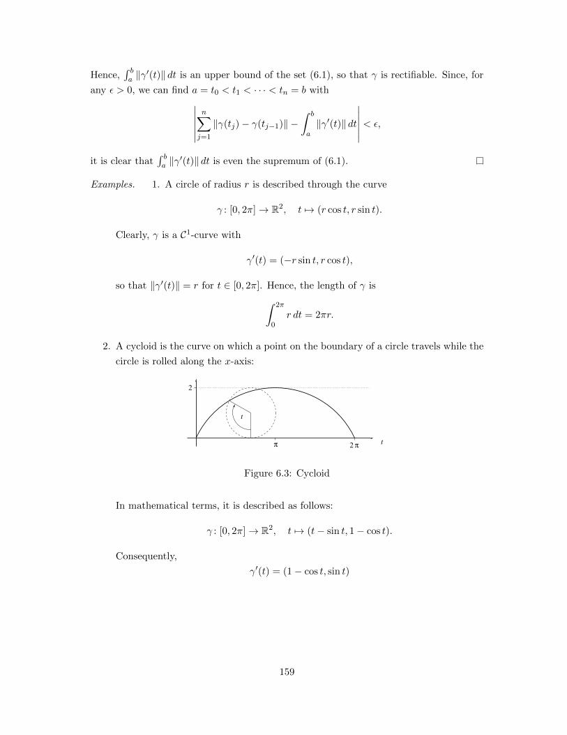
Hence,∫ ba ‖γ
′(t)‖ dt is an upper bound of the set (6.1), so that γ is rectifiable. Since, for
any ε > 0, we can find a = t0 < t1 < · · · < tn = b with∣∣∣∣∣∣n∑j=1
‖γ(tj)− γ(tj−1)‖ −∫ b
a‖γ′(t)‖ dt
∣∣∣∣∣∣ < ε,
it is clear that∫ ba ‖γ
′(t)‖ dt is even the supremum of (6.1).
Examples. 1. A circle of radius r is described through the curve
γ : [0, 2π]→ R2, t 7→ (r cos t, r sin t).
Clearly, γ is a C1-curve with
γ′(t) = (−r sin t, r cos t),
so that ‖γ′(t)‖ = r for t ∈ [0, 2π]. Hence, the length of γ is∫ 2π
0r dt = 2πr.
2. A cycloid is the curve on which a point on the boundary of a circle travels while the
circle is rolled along the x-axis:
2 π
2
πt
t
Figure 6.3: Cycloid
In mathematical terms, it is described as follows:
γ : [0, 2π]→ R2, t 7→ (t− sin t, 1− cos t).
Consequently,
γ′(t) = (1− cos t, sin t)
159

holds and thus
‖γ′(t)‖2 = (1− cos t)2 + (sin t)2
= 1− 2 cos t+ (cos t)2 + (sin t)2
= 2− 2 cos t
= 2− 2 cos
(t
2+t
2
)= 2− 2 cos
(t
2
)2
+ 2 sin
(t
2
)2
= 2
(sin
(t
2
)2
+ sin
(t
2
)2)
= 4 sin
(t
2
)2
for t ∈ [0, 2π]. Therefore, γ has the length∫ 2π
02
∣∣∣∣sin( t2)∣∣∣∣ dt = 4
∫ π
0sinu du = 8.
3. The first example is a very natural, but not the only way to describe a circle. Here
is another one:
γ : [0,√
2π]→ R2, t 7→ (r cos(t2), r sin(t2)).
Then
γ′(t) = (−2rt sin(t2), 2rt cos(t2)),
so that
‖γ′(t)‖ =√
4r2t2 (sin(t2)2 + cos(t2)2) = 2rt
holds for t ∈ [0,√
2π]. Hence, we obtain as length:∫ √2π
0‖γ′(t)‖ dt =
∫ √2π
02rt dt = 2r
t2
2
∣∣∣∣t=√
2π
t=0
= 2πr,
which is the same as in the first example.
Theorem 6.1.5. Let γ : [a, b]→ RN be a C1-curve, and let φ : [α, β]→ [a, b] be a bijective
C1-function. Then γ ◦ φ is a C1-curve with the same length as γ.
Proof. First, consider the case where φ is increasing, i.e., φ′ ≥ 0. It follows that∫ β
α‖(γ ◦ φ)′(t)‖ dt =
∫ β
α‖(γ′ ◦ φ)(t)φ′(t)‖ dt
=
∫ β
α‖(γ′ ◦ φ)(t)‖φ′(t) dt
=
∫ φ(β)=b
φ(α)=a‖γ′(s)‖ ds.
160

Suppose now that φ is decreasing, meaning that φ′ ≤ 0. We obtain∫ β
α‖(γ ◦ φ)′(t)‖ dt =
∫ β
α‖(γ′ ◦ φ)(t)φ′(t)‖ dt
= −∫ β
α‖(γ′ ◦ φ)(t)‖φ′(t) dt
= −∫ φ(β)=a
φ(α)=b‖γ′(s)‖ ds
=
∫ b
a‖γ′(s)‖ ds.
This completes the proof.
The theorem and its proof extend easily to piecewise C1-curves.
Next, we turn to defining (and computing) the angle between two curves:
Definition 6.1.6. Let γ : [a, b]→ RN be a C1-curve. The vector γ′(t) is called the tangent
vector to γ at t. If γ′(t) 6= 0, γ is called regular at t and singular at t otherwise. If γ′(t) 6= 0
for all t ∈ [a, b], we simply call γ regular.
Definition 6.1.7. Let γ1 : [a1, b1]→ RN and γ2 : [a2, b2]→ RN be two C1-curves, and let
t1 ∈ [a1, b1] and t2 ∈ [a2, b2] be such that:
(a) γ1 is regular at t1;
(b) γ2 is regular at t2;
(c) γ1(t1) = γ2(t2).
Then the angle between γ1 and γ2 at γ1(t1) = γ2(t2) is the unique θ ∈ [0, π] such that
cos θ =γ′1(t1) · γ′2(t2)
‖γ′1(t1)‖‖γ′2(t2)‖.
Loosely speaking, the angle between two curves is the angle between the corresponding
tangent vectors:
161

γ 1
γ 2
γ 1 t1( ) γ 2 t2( )=
θ
Figure 6.4: Angle between two curves
Example. Let
γ1 : [0, 2π]→ R2, t 7→ (cos t, sin t)
and
γ2 : [−1, 2]→ R2, t 7→ (t, 1− t).
We wish to find the angle between γ1 and γ2 at all points where the two curves intersect.
Since
‖γ2(t)‖2 = 2t2 − 2t+ 1 = (2t− 2)t+ 1
for all t ∈ [−1, 2], it follows that ‖γ2(t)‖ > 1 for all t ∈ [−1, 2] with t > 1 or t < 0 and
‖γ2(t)‖ < 1 for all t ∈ (0, 1), whereas γ2(0) = (0, 1) and γ2(1) = (1, 0) both have norm
one and thus lie on {γ1}. Consequently, we have
{γ1} ∩ {γ2} ={
(0, 1) = γ2(0) = γ1
(π2
), (1, 0) = γ2(1) = γ1(0)
}.
Let θ and σ denote the angle between γ1 and γ2 at (0, 1) and (1, 0), respectively. Since
γ′1(t) = (− sin t, cos t) and γ′2(t) = (1,−1)
for all t in the respective parameter intervals, we conclude that
cos θ =γ′1(π2
)· γ′2(0)∥∥γ′1 (π2 )∥∥ ‖γ′2(0)‖
=(−1, 0) · (1,−1)√
2= − 1√
2
and
cosσ =γ′1(0) · γ′2(1)
‖γ′1(0)‖‖γ′2(1)‖=
(0, 1) · (1,−1)√2
= − 1√2,
so that θ = σ = 3π4 .
162
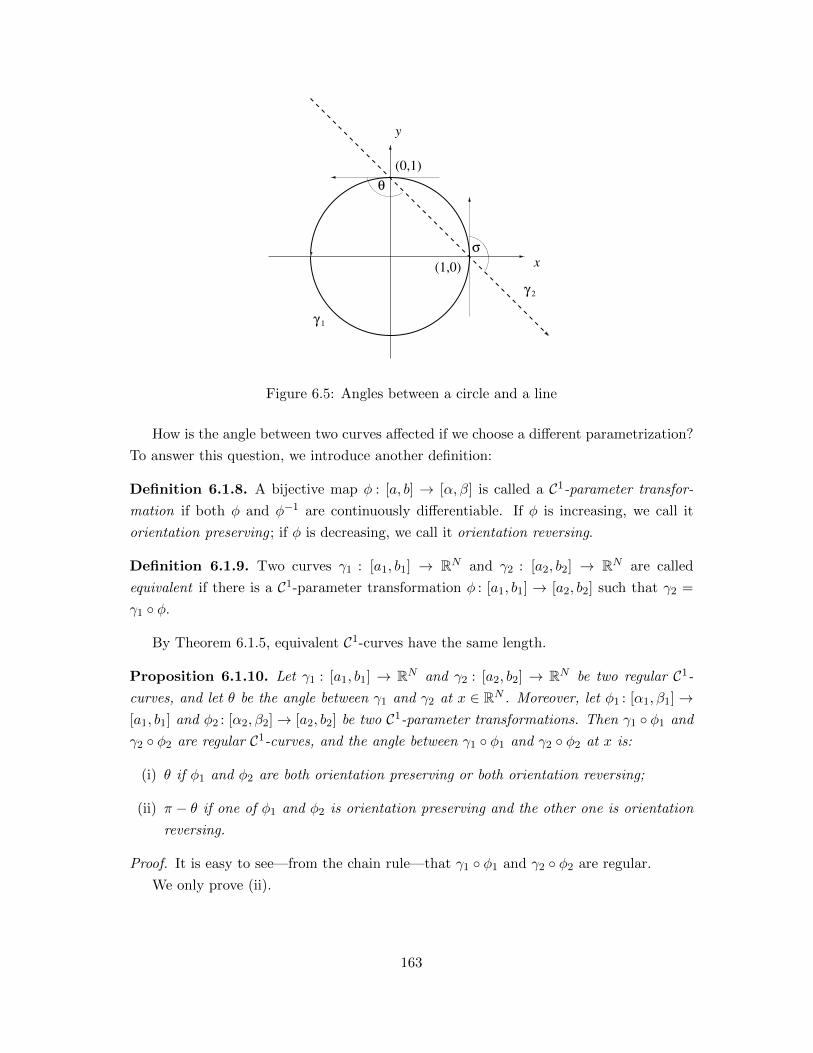
γ 1
γ 2
x
y
σ
θ
(0,1)
(1,0)
Figure 6.5: Angles between a circle and a line
How is the angle between two curves affected if we choose a different parametrization?
To answer this question, we introduce another definition:
Definition 6.1.8. A bijective map φ : [a, b] → [α, β] is called a C1-parameter transfor-
mation if both φ and φ−1 are continuously differentiable. If φ is increasing, we call it
orientation preserving ; if φ is decreasing, we call it orientation reversing.
Definition 6.1.9. Two curves γ1 : [a1, b1] → RN and γ2 : [a2, b2] → RN are called
equivalent if there is a C1-parameter transformation φ : [a1, b1] → [a2, b2] such that γ2 =
γ1 ◦ φ.
By Theorem 6.1.5, equivalent C1-curves have the same length.
Proposition 6.1.10. Let γ1 : [a1, b1] → RN and γ2 : [a2, b2] → RN be two regular C1-
curves, and let θ be the angle between γ1 and γ2 at x ∈ RN . Moreover, let φ1 : [α1, β1]→[a1, b1] and φ2 : [α2, β2]→ [a2, b2] be two C1-parameter transformations. Then γ1 ◦ φ1 and
γ2 ◦ φ2 are regular C1-curves, and the angle between γ1 ◦ φ1 and γ2 ◦ φ2 at x is:
(i) θ if φ1 and φ2 are both orientation preserving or both orientation reversing;
(ii) π − θ if one of φ1 and φ2 is orientation preserving and the other one is orientation
reversing.
Proof. It is easy to see—from the chain rule—that γ1 ◦ φ1 and γ2 ◦ φ2 are regular.
We only prove (ii).
163

For j = 1, 2, let tj ∈ [αj , βj ] be such that γ1(φ1(t1)) = γ2(φ2(t2)) = x. Suppose that
φ1 preserves orientation and that φ2 reverses it. We obtain
(γ1 ◦ φ1)′(t1) · (γ2 ◦ φ2)′(t2)
‖(γ1 ◦ φ1)′(t1)‖‖(γ2 ◦ φ2)′(t2)‖=
γ′1(φ1(t1))φ′1(t1) · γ′2(φ2(t2))φ′2(t2)
‖γ′1(φ1(t1))φ′1(t1)‖‖γ′2(φ2(t2))φ′2(t2)‖
=φ′1(t1)φ′2(t2)
−φ′1(t1)φ′2(t2)
γ′1(φ1(t1)) · γ′2(φ2(t2))
‖γ′1(φ1(t1))‖‖γ′2(φ2(t2))‖
= − γ′1(φ1(t1)) · γ′2(φ2(t2))
‖γ′1(φ1(t1))‖‖γ′2(φ2(t2))‖= − cos θ
= cos(π − θ),
which proves the claim.
Exercises
1. Let r > 0, and let c 6= 0. Determine the length of the helix
γ : [a, b]→ R3, t 7→ (r cos t, r sin t, ct).
2. (a) Let γj : [a, b]→ RN and γ2 : [b, c]→ RN be two curves such that γ1(b) = γ2(b).
The concatenation of γ1 and γ2 is the curve
γ1 ⊕ γ2 : [a, c]→ RN , t 7→
{γ1(t), if t ∈ [a, b],
γ2(t), if t ∈ [b, c].
Show that γ1 ⊕ γ2 is rectifiable provided that γ1 and γ2 are and that
length of γ1 ⊕ γ2 = length of γ1 + length of γ2.
(b) A curve γ : [a, b] → RN is called piecewise continuously differentiable—or
short: piecewise C1—if there is a partition a = t0 < · · · < tn = b such that
γj := γ|[tj−1,tj ] is continuously differentiable for j = 1, . . . , n. Show that γ is
rectifiable and that
length of γ =n∑j=1
∫ tj
tj−1
‖γ′j(t)‖ dt.
3. Parametrization with respect to arclength. Let γ : [a, b]→ RN be a regular C1-curve
with length L. Show that
τ : [a, b]→ [0, L], t 7→∫ t
a‖γ′(s)‖ ds
is a C1-parameter transformation. Conclude that there is a C1-curve γ : [0, L]→ RN
such that γ = γ ◦ τ .
164

4. Let
γ : R→ R2, t 7→ (t2 − 1, t3 − t).
(a) Sketch γ|[−2,2].
(b) Determine all s 6= t such that γ(s) = γ(t).
(c) Calculate the angle between γ and itself at all points γ(s) = γ(t) with s 6= t.
5. Show that
γ : [0, 1]→ R2, t 7→
{ (1, t cos
(πt
)), t ∈ (0, 1],
(1, 0), t = 0,
defines a curve that fails to be rectifiable. (Hint : Consider partitions 0 < 12n <
12n−1 < · · · <
13 <
12 < 1.)
6. Show that the following are equivalent for an open set U ⊂ RN :
(i) U is connected;
(ii) U is path connected;
(iii) any two points in U can be joined by a polygonal path in U , i.e., for any
x1, x2 ∈ U , there are a < b and a polygonal path γ : [a, b] → U such that
γ(a) = x1 and γ(b) = x2.
(Hint : For (i) =⇒ (iii), fix x1 ∈ U and consider the set of those x ∈ U such that x1
and x can be joined by a polygonal path in U .)
6.2 Curve Integrals
Let v : R3 → R3 be a force field, i.e., at each point x ∈ R3, the force v(x) is exerted. This
force field moves a particle along a curve γ : [a, b]→ R3. We would like to know the work
done in the process.
If γ is just a line segment and v is constant, this is easy:
work = v · (γ(b)− γ(a)).
For general γ and v, choose points γ(tj) and γ(tj−1) on γ so close that γ is “almost” a
line segment and that v is “almost” constant between those points. The work done by v
to move the particle from γ(tj−1) to γ(tj) is then approximately v(ηj) · (γ(tj)− γ(tj−1)),
for any ηj on γ “between” γ(tj−1) and γ(tj). For the the total amount of work, we thus
obtain
work ≈n∑j=1
v(ηj) · (γ(tj)− γ(tj−1)).
165
The finer we choose the partition a = t0 < t1 < · · · < tn = b, the better this approximation
of the work done should become.
These considerations, motivate the following definition:
Definition 6.2.1. Let γ : [a, b] → RN be a curve, and let f : {γ} → RN be a function.
Then f is said to be integrable along γ, if there is I ∈ R such that, for each ε > 0, there is
δ > 0 such that, for each partition a = t0 < t1 < · · · < tn = b with maxj=1,...,n(tj−tj−1) <
δ, we have ∣∣∣∣∣∣I −n∑j=1
f(γ(ξj)) · (γ(tj)− γ(tj−1))
∣∣∣∣∣∣ < ε
for each choice ξj ∈ [tj−1, tj ] for j = 1, . . . , n. The number I is called the (curve) integral
of f along γ and denoted by∫γf · dx or
∫γf1 dx1 + · · ·+ fN dxN .
Theorem 6.2.2. Let γ : [a, b] → RN be a rectifiable curve, and let f : {γ} → RN be
continuous. Then∫γ f · dx exists.
We will not prove this theorem.
Proposition 6.2.3. The following properties of curve integrals hold:
(i) Let γ : [a, b]→ RN and f, g : {γ} → RN be such that∫γ f · dx and
∫γ g · dx both exist,
and let α, β ∈ R. Then∫γ(α f + β g) · dx exists such that∫
γ(α f + β g) · dx = α
∫γf · dx+ β
∫γg · dx.
(ii) Let γ1 : [a, b] → RN , γ2 : [b, c] → RN and f : {γ1} ∪ {γ2} → RN be such that
γ1(b) = γ2(b) and that∫γ1f · dx and
∫γ2f · dx both exist. Then
∫γ1⊕γ2 f · dx exists
such that ∫γ1⊕γ2
f · dx =
∫γ1
f · dx+
∫γ2
f · dx.
(iii) Let γ : [a, b]→ RN be rectifiable, and let f : {γ} → RN be bounded such that∫γ f · dx
exists. Then ∣∣∣∣∫γf · dx
∣∣∣∣ ≤ sup{‖f(γ(t))‖ : t ∈ [a, b]} · length of γ
holds.
166

Proof. (Only of (iii)).
Let ε > 0, and choose are partition a = t0 < t1 < · · · < tn = b such that∣∣∣∣∣∣∫γf · dx−
n∑j=1
f(γ(tj)) · (γ(tj)− γ(tj−1))
∣∣∣∣∣∣ < ε.
It follows that∣∣∣∣∫γf · dx
∣∣∣∣ ≤∣∣∣∣∣∣n∑j=1
f(γ(tj)) · (γ(tj)− γ(tj−1))
∣∣∣∣∣∣+ ε
≤n∑j=1
‖f(γ(tj))‖‖γ(tj)− γ(tj−1)‖+ ε
≤ sup{‖f(γ(t))‖ : t ∈ [a, b]} ·n∑j=1
‖γ(tj)− γ(tj−1)‖+ ε
≤ sup{‖f(γ(t))‖ : t ∈ [a, b]} · length of γ + ε.
Since ε > 0 was arbitrary, this yields (iii).
Theorem 6.2.4. Let γ : [a, b]→ RN be a C1-curve, and let f : {γ} → RN be continuous.
Then ∫γf · dx =
∫ b
af(γ(t)) · γ′(t) dt
holds.
Proof. Let ε > 0, and choose δ1 > 0 such that, for each partition a = t0 < t1 < · · · < tn = b
with maxj=1,...,n(tj − tj−1) < δ1 and for any choice ξj ∈ [tj−1, tj ] for j = 1, . . . , n, we have∣∣∣∣∣∣∫ b
af(γ(t)) · γ′(t) dt−
n∑j=1
f(γ(ξj)) · γ′(ξj)(tj − tj−1)
∣∣∣∣∣∣ < ε
2.
Let C > 0 be such that C ≥ sup{‖f(γ(t))‖ : t ∈ [a, b]}, and choose δ2 > 0 such that∥∥∥∥γ(t)− γ(s)
t− s− γ′(t)
∥∥∥∥ < ε
4C(b− a)
for s, t ∈ [a, b] with 0 < |s − t| < δ2. Since γ′ is uniformly continuous, we may choose δ2
so small that
‖γ′(t)− γ′(s)‖ < ε
4C(b− a)
167

for s, t ∈ [a, b] with |s−t| < δ2. Consequently, we obtain for s, t,∈ [a, b] with 0 < t−s < δ2
and for ξ ∈ [s, t] that∥∥∥∥γ(t)− γ(s)
t− s− γ′(ξ)
∥∥∥∥ ≤ ∥∥∥∥γ(t)− γ(s)
t− s− γ′(t)
∥∥∥∥+ ‖γ′(t)− γ′(ξ)‖
<ε
4C(b− a)+
ε
4C(b− a)
=ε
2C(b− a)(6.2)
Let δ := min{δ1, δ2}, and choose a partition a = t0 < t1 < · · · < tn = b with
maxj=1,...,n(tj − tj−1) < δ. From (6.2), we obtain:
‖(γ(tj)− γ(tj−1))− γ′(ξj)(tj − tj−1)‖ < ε
2C
tj − tj−1
b− a(6.3)
for any choice of ξj ∈ [tj−1, tj ] for j = 1, . . . , n. Moreover, we have∣∣∣∣∣∣∫ b
af(γ(t)) · γ′(t) dt−
n∑j=1
f(γ(ξj)) · (γ(tj)− γ(tj−1))
∣∣∣∣∣∣≤
∣∣∣∣∣∣∫ b
af(γ(t)) · γ′(t) dt−
n∑j=1
f(γ(ξj)) · γ′(ξj)(tj − tj−1)
∣∣∣∣∣∣+
∣∣∣∣∣∣n∑j=1
f(γ(ξj)) · γ′(ξj)(tj − tj−1)−n∑j=1
f(γ(ξj)) · (γ(tj)− γ(tj−1))
∣∣∣∣∣∣<ε
2+
n∑j=1
|f(γ(ξj)) · (γ′(ξj)(tj − tj−1)− (γ(tj)− γ(tj−1)))|
≤ ε
2+
n∑j=1
‖f(γ(ξj))‖‖γ′(ξj)(tj − tj−1)− (γ(tj)− γ(tj−1))‖
<ε
2+
n∑j=1
Cε
2C
tj − tj−1
b− a, by (6.3),
=ε
2+ε
2
= ε.
By the definition of a curve integral, this yields the claim.
Of course, this theorem has an obvious extension to piecewise C1-curves.
Example. Let
γ : [0, 4π]→ R3, t 7→ (cos t, sin t, t),
and let
f : R3 → R3, (x, y, z) 7→ (1, cos z, xy).
168
It follows that ∫γf · d(x, y, z) =
∫γ
1 dx+ cos z dy + xy dz
=
∫ 4π
0(1, cos t, cos t sin t) · (− sin t, cos t, 1) dt
=
∫ 4π
0(− sin t+ (cos t)2 + (cos t)(sin t)) dt
=
∫ 4π
0(cos t)2 dt
= 2π.
We next turn to how a change of parameters affects curve integrals:
Proposition 6.2.5. Let γ : [a, b] → RN be a piecewise C1-curve, let f : {γ} → RN be
continuous, and let φ : [α, β] → [a, b] be a C1-parameter transformation. Then, if φ is
orientation preserving, ∫γ◦φ
f · dx =
∫γf · dx
holds, and ∫γ◦φ
f · dx = −∫γf · dx
holds if φ is orientation reversing.
Proof. Without loss of generality, suppose that γ is a C1-curve.
We only prove the assertion for orientation reversing φ.
Simply note that ∫γ◦φ
f · dx =
∫ β
αf(γ(φ(t))) · (γ ◦ φ)′(t) dt
=
∫ β
αf(γ(φ(t))) · γ′(φ(t))φ′(t) dt
=
∫ a
bf(γ(s)) · γ′(s) ds
= −∫ b
af(γ(s)) · γ′(s) ds
= −∫γf · dx.
This proves the claim.
We introduce new terminology:
Definition 6.2.6. Let ∅ 6= U ⊂ RN be open. We call a vector field f : U → RN
conservative with potential function F : U → R if F is partially differentiable such that
f = ∇F .
169

We previously encountered conservative vector fields under the name gradient fields.
Theorem 6.2.7 (Fundamental Theorem for Curve Integrals). Let ∅ 6= U ⊂ RN be
open, let f : U → RN be a continuous, conservative vector field with potential function
F : U → R, and let γ : [a, b]→ U be a piecewise C1-curve. Then∫γf · dx = F (γ(b))− F (γ(a))
holds.
Proof. Choose a = t0 < t1 < · · · < tn = b such that γ|[tj−1,tj ] is continuously differentiable
for j = 1, . . . , n. We then obtain∫γf · dx =
∫γ∇F · dx
=n∑j=1
∫ tj
tj−1
N∑k=1
∂F
∂xk(γ(t))γ′k(t) dt
=n∑j=1
∫ tj
tj−1
d
dtF (γ(t)) dt
=
n∑j=1
(F (γ(tj))− F (γ(tj−1)))
= F (γ(b))− F (γ(a)),
as claimed.
Remark. The adjective “conservative” for gradient fields derives itself from the Law of
Conservation of Energy. Suppose that N = 3 and that f moves a particle of mass m
along a curve γ : [a, b]→ R3. We suppose that γ is twice continuously differentiable. Then
Newton’s Second Law of Motion yields that
f(γ(t)) = mγ′′(t)
for t ∈ [a, b]. Consequently, the work carried out is computed as
work =
∫γf · dx
=
∫ b
af(γ(t)) · γ′(t) dt
= m
∫ b
aγ′′(t) · γ′(t) dt
=m
2
∫ b
a
d
dt‖γ′(t)‖2 dt
=m
2(‖γ′(b)‖2 − ‖γ′(a)‖2).
170
For t ∈ [a, b], the kinetic energy at γ(t) is
K(γ(t)) =m
2‖γ′(t)‖2,
so that
work = K(γ(b))−K(γ(a)).
Suppose now that f is conservative with potential function F . Then the potential energy
at (x, y, z) is P (x, y, z) = −F (x, y, z), so that
work =
∫γf · dx = F (γ(b))− F (γ(a)) = P (γ(a))− P (γ(b)).
by Theorem 6.2.7. All in all, we obtain
P (γ(a)) +K(γ(a)) = P (γ(b)) +K(γ(b)),
i.e., the Law of Conservation of Energy.
Example. Let
f : R3 → R3, (x, y, z) 7→ (2xz,−1, x2),
and let γ : [a, b]→ R3 be any piecewise C1-curve with γ(a) = (−4, 6, 1) and γ(b) = (3, 0, 1).
Since f is the gradient of
F : R3 → R, (x, y, z) 7→ x2z − y,
Theorem 6.2.7 yields that∫γf · dx = F (3, 0, 1)− F (−4, 6, 1) = 10− 9 = 1.
Theorem 6.2.7 greatly simplifies the calculation of curve integrals of conservative vector
fields. Not every vector field, however, is conservative as we shall see very soon.
To make formulations easier, we define:
Definition 6.2.8. A curve γ : [a, b]→ RN is called closed if γ(a) = γ(b).
Corollary 6.2.9. Let ∅ 6= U ⊂ RN be open, and let f : U → RN be a continuous,
conservative vector field. Then∫γ f · dx = 0 holds for every closed, piecewise C1-curve γ
in U .
Example. Let P,Q : R2 \ {(0, 0)} → R be given by
P (x, y) = − y
x2 + y2and Q(x, y) =
x
x2 + y2
for (x, y) ∈ R2 \ {(0, 0)}. Consider the counterclockwise oriented unit circle
γ : [0, 2π]→ R2, t 7→ (cos t, sin t);
171
in particular, γ is a closed C1-curve. A direct evaluation yields∫γP dx+Qdy =
∫ 2π
0(P (γ(t)), Q(γ(t))) · γ′(t) dt
=
∫ 2π
0(− sin t, cos t) · (− sin t, cos t) dt
=
∫ 2π
0sin2 t+ cos2 t dt
= 2π,
so that (P,Q) cannot be conservative.
Under certain circumstances, a converse of Corollary 6.2.9 is true:
Theorem 6.2.10. Let ∅ 6= U ⊂ RN be open and convex, and let f : U → RN be
continuous. Then the following are equivalent:
(i) f is conservative;
(ii)∫γ f · dx = 0 for each closed, piecewise C1-curve γ in U .
Proof. (i) =⇒ (ii) is Corollary 6.2.9.
(ii) =⇒ (i): For any x, y ∈ U , define
[x, y] := {x+ t(y − x) : t ∈ [0, 1]}.
Since U is convex, we have [x, y] ⊂ U . Clearly, [x, y] can be parametrized as a C1-curve:
[0, 1]→ RN , t 7→ x+ t(y − x).
Fix x0 ∈ U , and define
F : U → R, x 7→∫
[x0,x]f · dx.
Let x ∈ U , and let ε > 0 be such that Bε(x) ⊂ U . Let h 6= 0 be such that ‖h‖ < ε.
We obtain
F (x+ h)− F (x) =
∫[x0,x+h]
f · dx−∫
[x0,x]f · dx
=
∫[x0,x+h]
f · dx−∫
[x,x+h]f · dx+
∫[x,x+h]
f · dx−∫
[x0,x]f · dx
=
∫[x0,x+h]
f · dx+
∫[x+h,x]
f · dx+
∫[x,x0]
f · dx+
∫[x,x+h]
f · dx
=
∫[x0,x+h]⊕[x+h,x]⊕[x,x0]
f · dx︸ ︷︷ ︸=0
+
∫[x,x+h]
f · dx
=
∫[x,x+h]
f · dx.
172

x 0[ ,x]
x 0 x+ h [ , ]
x+ h [x , ]x+ h
x 0
U
x
Figure 6.6: Integration curves in the proof of Theorem 6.2.10
It follows that
1
‖h‖|F (x+ h)− F (x)− f(x) · h| = 1
‖h‖
∣∣∣∣∣∫
[x,x+h]f · dx−
∫[x,x+h]
f(x) · dx
∣∣∣∣∣=
1
‖h‖
∣∣∣∣∣∫
[x,x+h](f − f(x)) · dx
∣∣∣∣∣ ≤ sup{‖f(y)− f(x)‖ : y ∈ [x, x+ h]}. (6.4)
Since f is continuous at x, the right hand side of (6.4) tends to zero as h→ 0.
This theorem remains true for general open, connected sets: the given proof can be
adapted to this more general situation (see Exercise 3 below).
Even though Theorem 6.2.10 is important, it is of little use to determine whether or
not a given vector field is conservative. The next proposition gives a necessary condition:
Proposition 6.2.11. Let ∅ 6= U ⊂ RN be open, and let f = (f1, . . . , fN ) : U → RN be a
conservative C1-vector field. Then∂fj∂xk
=∂fk∂xj
(6.5)
holds on U for j, k = 1, . . . , N .
Remark. If N = 3, then (6.5) amounts to curl f = 0.
Proof. Let F : U → R be a potential function for f . As f is a C1-vector field, it follows
that F is twice continuously partially differentiable. Hence, we obtain from Clairaut’s
Theorem that∂fj∂xk
=∂2F
∂xk∂xj=
∂2F
∂xj∂xk=∂fk∂xj
on U for j, k = 1, . . . , N .
173

Alas, (6.5) need not be sufficient for a vector field to be conservative:
Example. Let P,Q : R2 \ {(0, 0)} → R be given by
P (x, y) = − y
x2 + y2and Q(x, y) =
x
x2 + y2
for (x, y) ∈ R2 \ {(0, 0)}. Then the rules of differentiation yield
∂P
∂y= − 1
x2 + y2+
2y2
(x2 + y2)2=−x2 − y2 + 2y2
(x2 + y2)2=−x2 + y2
(x2 + y2)2
and∂Q
∂x=
1
x2 + y2− 2x2
(x2 + y2)2=x2 + y2 − 2x2
(x2 + y2)2=−x2 + y2
(x2 + y2)2,
so that the vector field (P,Q) satisfies (6.5). However, as we have previously seen, (P,Q)
is not conservative.
Still, for sufficiently “nice” domains, a converse of Proposition 6.2.11 holds. To prove
it, we require some preparations.
Proposition 6.2.12. Let f : [a, b]× [c, d]→ R be continuous, and define
F : [a, b]→ R, x 7→∫ d
cf(x, y) dy.
Then F is continuous.
Proof. Let x0 ∈ [a, b], and let ε > 0. Choose δ > 0 such that
|f(x, y)− f(x′, y′)| < ε
d− cfor all (x, y), (x′, y′) ∈ [a, b] × [c, d] such that ‖(x, y) − (x′, y′)‖ < δ. (Remember: since
[a, b]× [c, d] is compact, f is uniformly continuous.) For x ∈ [a, b] such that |x− x0| < δ,
we thus obtain
|F (x)− F (x0)| =∣∣∣∣∫ d
cf(x, y) dy −
∫ d
cf(x0, y) dy
∣∣∣∣ ≤ ∫ d
c|f(x, y)− f(x0, y)|︸ ︷︷ ︸
< εd−c
dy ≤ ε,
which proves the claim.
Theorem 6.2.13. Let f : [a, b] × [c, d] → R be continuous, and suppose further that ∂f∂x
exists and is continuous throughout. Define
F : [a, b]→ R, x 7→∫ d
cf(x, y) dy.
Then F is continuously differentiable such that
F ′(x) =
∫ d
c
∂f
∂x(x, y) dy
for x ∈ [a, b].
174

Proof. Let ε > 0. Choose δ > 0 such that∣∣∣∣∂f∂x (x, y)− ∂f
∂x(x′, y′)
∣∣∣∣ < ε
d− c
for all (x, y), (x′, y′) ∈ [a, b]× [c, d] with ‖(x, y)− (x′, y′)‖ < δ. Fix x0 ∈ [a, b] and y ∈ [c, d],
and let h 6= 0 be such that x0 +h ∈ [a, b] and |h| < δ. By the Intermediate Value Theorem,
there is ξy between x0 and x0 + h such that
f(x0 + h, y)− f(x0, y)
h=∂f
∂x(ξy, y).
As ‖(x0, y)− (ξy, y)‖ < δ, we have∣∣∣∣f(x0 + h, y)− f(x0, y)
h− ∂f
∂x(x0, y)
∣∣∣∣ =
∣∣∣∣∂f∂x (ξy, y)− ∂f
∂x(x0, y)
∣∣∣∣ < ε
d− c.
Hence, it follows for 0 < |h| < δ such that x0 + h ∈ [a, b] that∣∣∣∣F (x0 + h)− F (x0)
h−∫ d
c
∂f
∂x(x0, y) dy
∣∣∣∣≤∫ d
c
∣∣∣∣f(x0 + h, y)− f(x0, y)
h− ∂f
∂x(x0, y)
∣∣∣∣︸ ︷︷ ︸< εd−c
dy ≤ ε.
We conclude that
limh→0h6=0
F (x0 + h)− F (x0)
h=
∫ d
c
∂f
∂x(x0, y) dy,
so that F is differentiable at x0 with
F ′(x0) =
∫ d
c
∂f
∂x(x0, y) dy
As x0 ∈ U is arbitrary, we obtain from Proposition 6.2.12 that F ′ is continuous as claimed.
Corollary 6.2.14. Let ∅ 6= U ⊂ RN be open, and let f : U × [a, b] → R be continuous
such that ∂f∂xj
exists and is continuous throughout for j = 1, . . . , N . Then
F : U → R, (x1, . . . , xN ) 7→∫ b
af(x1, . . . , xN , y) dy
is continuously partially differentiable such that
∂F
∂xj(x) =
∫ b
a
∂f
∂xj(x, y) dy
for x ∈ U and j = 1, . . . , N .
175

This allows us to prove a converse to Proposition 6.2.11.
Theorem 6.2.15. Let ∅ 6= U ⊂ RN be open, and let f : U → RN be a C1-vector field.
Consider the following statements:
(i) f is conservative;
(ii) f satisfies (6.5).
Then (i) =⇒ (ii), and (ii) =⇒ (i) if there is x0 ∈ U such that [x0, x] ⊂ U for all x ∈ U .
Remark. Sets satisfying the condition for (ii) =⇒ (i) to hold are called star shaped : think
of a star with x0 as its geometric center. Every convex set is trivially star shaped, but it
is easy to come up with star shaped sets that are not convex (see Exercise 1.4.7).
Proof. (i) =⇒ (ii) is clear by Proposition 6.2.11.
Suppose that f satisfies (6.5) and that U is star shaped. Without loss of generality,
suppose that x0 = 0. Define
F : U → R, x 7→∫
[0,x]f · dx,
so that
F (x) =N∑j=1
(∫ 1
0fj(tx) dt
)xj
for x ∈ U . It follows for x ∈ U and k = 1, . . . , N that
∂F
∂xk(x) =
N∑j=1
(∂
∂xk
∫ 1
0fj(tx) dt
)xj +
N∑j=1
(∫ 1
0fj(tx) dt
)∂xj∂xk
=N∑j=1
(∫ 1
0t∂fj∂xk
(tx) dt
)xj +
∫ 1
0fk(tx) dt, by Corollary 6.2.14,
=
∫ 1
0
fk(tx) + tN∑j=1
∂fj∂xk
(tx)xj
dt. (6.6)
Also, note that
d
dttfk(tx) = fk(tx) + t
d
dtfk(tx)
= fk(tx) + t
N∑j=1
∂fk∂xj
(tx)xj
= fk(tx) + tN∑j=1
∂fj∂xk
(tx)xj , by (6.5), (6.7)
176

for x ∈ U and k = 1, . . . , N . Note that (6.7) is just the integrand of (6.6), so that
∂F
∂xk(x) =
∫ 1
0
d
dttfk(tx) dt = tfk(tx)
∣∣∣∣∣1
0
= fk(x)
for x ∈ U and k = 1, . . . , k.
Example. Let
f : R3 → R3, (x, y, z) 7→ (yexy, xexy, 1).
A routine calculation shows that curl f = 0, so that f is conservative. Let F : R3 → R be
a potential function for f . It follows that
F (x, y, z) =
∫1 dz = z +G(x, y).
Differentiation with respect to x and y yields
∂F
∂x(x, y) =
∂G
∂x(x, y) = yexy and
∂F
∂y(x, y) =
∂G
∂y(x, y) = xexy,
so that
G(x, y) =
∫xexy dy = exy +H(x).
Differentiating with respect to x, we obtain
∂G
∂x(x, y) = yexy +
dH
dx(x)
so that dHdx ≡ 0 and H is constant. It follows that
F (x, y, z) = exy + z + C
for some constant C.
Exercises
1. Let
f : R2 → R2, (x, y) 7→ (y, y − x) and g : R2 → R2, (x, y) 7→ (y, x− y).
Determine whether f or g are conservative. If so, determine a respective potential
function.
2. Let f = (P,Q,R) : R3 → R3 be given by
P (x, y, z) = eyz, Q(x, y, z) = xzeyz, and R(x, y, z) = xyeyz
177

for x, y, z ∈ R, and let
γ : [0, 6π]→ R, t 7→ (cos t, sin t, 666t).
Evaluate the curve integral ∫γP dx+Qdy +Rdz.
3. Generalize Theorem 6.2.10 to general open and connected ∅ 6= U ⊂ RN . For (ii)
=⇒ (i), proceed as follows:
• Show that, if γ and γ are piecewise C1-curves in U with same initial points and
endpoints, then∫γ f · dx =
∫γ f · x.
• Fix x0 ∈ U . By Exercise 6.1.6, there is, for each x ∈ U , a piecewise C1-curve
γx in U with initial point x0 and endpoint x. Show that
F : U → R, x 7→∫γx
f · dx
is well defined and a potential function for f .
6.3 Green’s Theorem
Definition 6.3.1. Let a < b, and let φ1, φ2 : [a, b]→ R be continuous with φ1 ≤ φ2. Then
{(x, y) ∈ R2 : x ∈ [a, b], φ1(x) ≤ y ≤ φ2(x)}, (6.8)
is called a normal domain in R2 with respect to the x-axis if, for j = 1, 2, there are αj < βj
and strictly increasing σj : [αj , βj ]→ R onto [a, b] such that
[αj , βj ]→ R2, t 7→ (σj(t), φj(σj(t)))
are piecewise C1-curves.
Remark. Of course, a set of the form (6.8) is a normal domain with respect to the x-axis
if φ1 and φ2 are piecewise C1-functions.
178
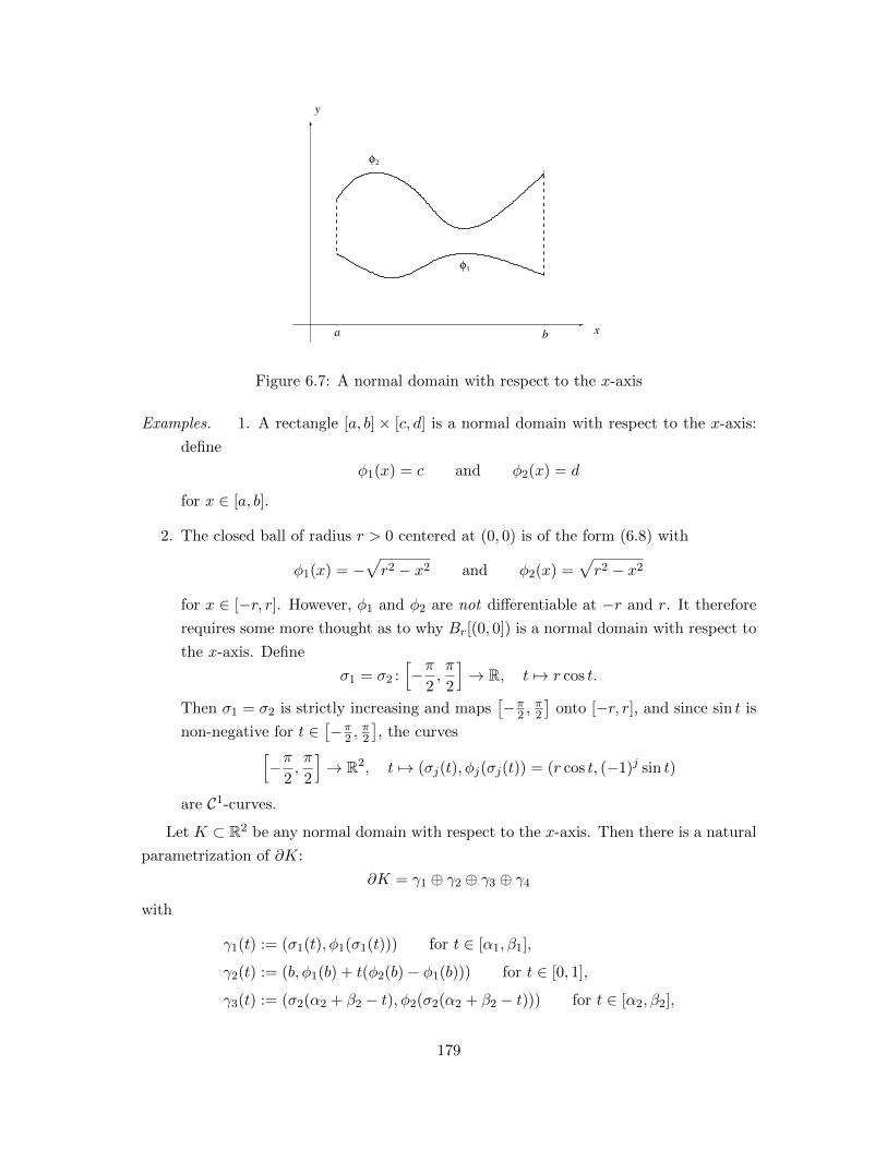
φ1
φ2
y
b xa
Figure 6.7: A normal domain with respect to the x-axis
Examples. 1. A rectangle [a, b] × [c, d] is a normal domain with respect to the x-axis:
define
φ1(x) = c and φ2(x) = d
for x ∈ [a, b].
2. The closed ball of radius r > 0 centered at (0, 0) is of the form (6.8) with
φ1(x) = −√r2 − x2 and φ2(x) =
√r2 − x2
for x ∈ [−r, r]. However, φ1 and φ2 are not differentiable at −r and r. It therefore
requires some more thought as to why Br[(0, 0]) is a normal domain with respect to
the x-axis. Define
σ1 = σ2 :[−π
2,π
2
]→ R, t 7→ r cos t.
Then σ1 = σ2 is strictly increasing and maps[−π
2 ,π2
]onto [−r, r], and since sin t is
non-negative for t ∈[−π
2 ,π2
], the curves[
−π2,π
2
]→ R2, t 7→ (σj(t), φj(σj(t)) = (r cos t, (−1)j sin t)
are C1-curves.
Let K ⊂ R2 be any normal domain with respect to the x-axis. Then there is a natural
parametrization of ∂K:
∂K = γ1 ⊕ γ2 ⊕ γ3 ⊕ γ4
with
γ1(t) := (σ1(t), φ1(σ1(t))) for t ∈ [α1, β1],
γ2(t) := (b, φ1(b) + t(φ2(b)− φ1(b))) for t ∈ [0, 1],
γ3(t) := (σ2(α2 + β2 − t), φ2(σ2(α2 + β2 − t))) for t ∈ [α2, β2],
179

and
γ4(t) := (a, φ2(a) + t(φ1(a)− φ2(a)) for t ∈ [0, 1].
γ 1
γ2
γ3γ
4
y
b xa
Figure 6.8: Natural parametrization of ∂K
We then say that ∂K is positively oriented.
Lemma 6.3.2. Let ∅ 6= U ⊂ R2 be open, let K ⊂ U be a normal domain with respect to
the x-axis, and let P : U → R be continuous such that ∂P∂y exists and is continuous. Then∫
K
∂P
∂y= −
∫∂K
P dx (+0 dy)
holds.
Proof. To simplify the bookkeeping, we only deal with the case where σ1 and σ2 are
C1-functions.
First note that∫K
∂P
∂y=
∫ b
a
(∫ φ2(x)
φ1(x)
∂P
∂y(x, y) dy
)dx, by Fubini’s Theorem,
=
∫ b
a(P (x, φ2(x))− P (x, φ1(x))) dx,
by the Fundamental Theorem of Calculus.
As a = σ1(α1) and b = σ1(β1), substituting x = σ1(t) yields∫ b
aP (x, φ1(x)) dx =
∫ β1
α1
P (σ1(t), φ1(σ1(t)))σ′1(t) dt =
∫ β1
α1
(P (γ1(t)), 0)·γ′1(t) dt =
∫γ1
P dx
180
Similarly, we obtain∫ b
aP (x, φ2(x)) dx =
∫ β2
α2
P (σ2(t), φ2(σ2(t)))σ′2(t) dt
= −∫ α2
β2
P (σ2(α2 + β2 − t), φ2(σ2(α2 + β2 − t)))σ′2(α2 + β2 − t) dt
=
∫ β2
α2
P (σ2(α2 + β2 − t), φ2(σ2(α2 + β2 − t)))σ′2(α2 + β2 − t) dt
= −∫ β2
α2
(P (γ3(t)), 0) · γ′3(t) dt
= −∫γ3
P dx.
It follows that ∫K
∂P
∂y= −
(∫γ1
P dx+
∫γ3
P dx
).
Since ∫γ2
P dx =
∫γ4
P dx = 0,
we eventually obtain ∫K
∂P
∂y= −
∫γ1⊕γ2⊕γ3⊕γ4
P dx = −∫∂K
P dx
as claimed.
As for the x-axis, we can define normal domains with respect to the y-axis:
Definition 6.3.3. Let c < d, and let ψ1, ψ2 : [c, d] → R be continuous with ψ1 ≤ ψ2.
Then
{(x, y) ∈ R2 : y ∈ [c, d], ψ1(y) ≤ x ≤ ψ2(y)},
is called a normal domain in R2 with respect to the y-axis if, for j = 1, 2, there are γj < δj
and strictly increasing τj : [γj , δj ]→ R onto [a, b] such that
[γj , δj ]→ R2, t 7→ (ψj(τj(t)), τj(t))
are piecewise C1-curves.
181

ψ2
ψ1
y
d
c
x
Figure 6.9: A normal domain with respect to the y-axis
Example. Rectangles and discs are normal domains with respect to the y-axis as well.
As for normal domains with respect to the x-axis, there is a canonical parametrization
for the boundary of every normal domain in R2 with respect to the x-axis. We then also
call the boundary with this parametrization positively oriented.
With an almost identical proof as for Lemma 6.3.2, we obtain:
Lemma 6.3.4. Let ∅ 6= U ⊂ R2 be open, let K ⊂ U be a normal domain with respect to
the y-axis, and let Q : U → R be continuous such that ∂Q∂x exists and is continuous. Then∫
K
∂Q
∂x=
∫∂K
(0 dx+)Qdy
holds.
Proof. As for Lemma 6.3.2.
Definition 6.3.5. A set K ⊂ R2 is called a normal domain if it is a normal domain with
respect to both the x- and the y-axis.
Theorem 6.3.6 (Green’s Theorem). Let ∅ 6= U ⊂ R2 be open, let K ⊂ U be a normal
domain, and let P,Q ∈ C1(U,R). Then∫K
(∂Q
∂x− ∂P
∂y
)=
∫∂K
P dx+Qdy
holds.
Proof. Add the identities in Lemmas 6.3.2 and 6.3.4.
182
Green’s Theorem is often useful to compute curve integrals:
Examples. 1. Let K = [0, 2]× [1, 3]. Then we obtain∫∂K
xy dx+ (x2 + y2) dy =
∫K
2x− x =
∫ 2
0
(∫ 3
1x dy
)dx = 4.
2. Let K = B1[(0, 0)]. Then we have∫∂K
xy2 dx+ (arctan(log y + 3)− x) dy
=
∫K−1− 2xy
= −∫K
2xy + 1
= −∫ 2π
0
(∫ 1
0(2r2 cos θ sin θ + 1)r dr
)dθ
= −(∫ 2π
0(cos θ)(sin θ) dθ
)︸ ︷︷ ︸
=0
(2
∫ 1
0r3 dr
)− 2π
∫ 1
0r dr
= −π.
Another nice consequence of Green’s Theorem is:
Corollary 6.3.7. Let K ⊂ R2 be a normal domain. Then
µ(K) =1
2
∫∂K
x dy − y dx
holds.
Proof. Apply Green’s Theorem with P (x, y) = −y and Q(x, y) = x.
Remark. Green’s Theorem remains valid for much more general domains than normal
ones. For instance, a triangle ∆ is normal if and only if one of its sides is parallel to one
of the coordinate axes. We can rotate ∆ suitably and obtain a triangle ∆ with a side
parallel to one of the coordinate axes:
183

∆~
y
x
∆
Figure 6.10: Rotating a triangle to obtain a normal domain
As ∆ is normal, we can apply Green’s Theorem to it. Change of Variables then yields
that Green’s Theorem holds for ∆ as well. When dealing with a tetrangle, e.g., a rectangle,
a trapeze, or a diamond, we split it into two triangles:
y
x
Figure 6.11: Splitting a tetrangle into two triangles
We can then apply Green’s Theorem to each of the two triangles. As the added bound-
ary piece is traversed twice, but in opposite directions, its contibutions to the boundary
integrals cancel each other. Hence, Green’s Theorem holds for general tetrangles. More
generally, Green’s Theorem applies to any polygon:
184

y
x
Figure 6.12: Splitting a polygon into triangles
Exercises
1. Show that
K := {(x, y) ∈ R2 : x, y, x+ y ∈ [0, 1]}
is a normal domain (with respect to both coordinate axes) and use Green’s Theorem
to compute ∫∂K
y ex dx+ x ey dy.
2. Let a, b > 0. Use Green’s Theorem to determine the area of the ellipse
E :=
{(x, y) ∈ R2 :
x2
a2+y2
b2≤ 1
}.
6.4 Surfaces in R3
What is the area of the surface of the Earth or—more generally—what is the surface area
of a sphere of radius r?
Before we can answer this question, we need, of course, make precise what we mean
by a surface
Definition 6.4.1. Let U ⊂ R2 be open, and let ∅ 6= K ⊂ U be compact and with content.
A surface with parameter domain K is the restriction of a C1-function Φ: U → R3 to K.
The set K is called the parameter domain of Φ, and {Φ} := Φ(K) is called the trace or
the surface element of Φ.
Examples. 1. Let r > 0, and let
Φ: R2 → R3, (s, t) 7→ (r(cos s)(cos t), r(sin s)(cos t), r sin t)
185
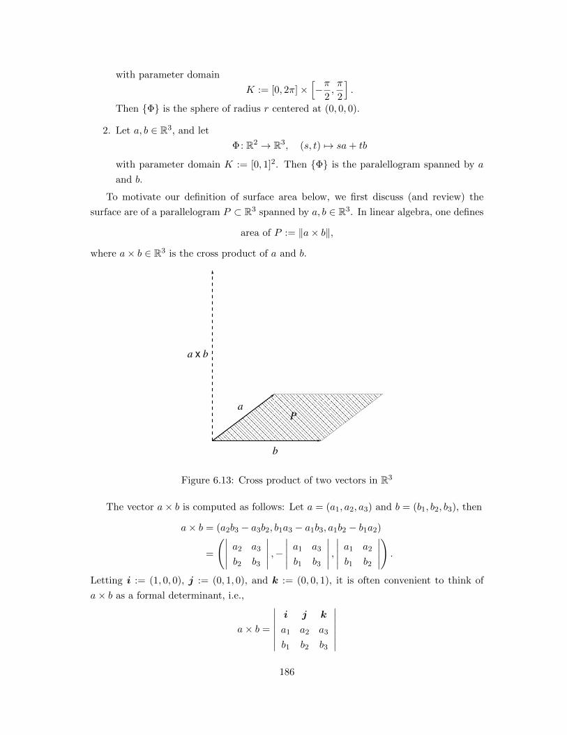
with parameter domain
K := [0, 2π]×[−π
2,π
2
].
Then {Φ} is the sphere of radius r centered at (0, 0, 0).
2. Let a, b ∈ R3, and let
Φ: R2 → R3, (s, t) 7→ sa+ tb
with parameter domain K := [0, 1]2. Then {Φ} is the paralellogram spanned by a
and b.
To motivate our definition of surface area below, we first discuss (and review) the
surface are of a parallelogram P ⊂ R3 spanned by a, b ∈ R3. In linear algebra, one defines
area of P := ‖a× b‖,
where a× b ∈ R3 is the cross product of a and b.
��������������������������������������������������������������������������������������������������������������������������������������������������������������������������������������������������������������������������������
��������������������������������������������������������������������������������������������������������������������������������������������������������������������������������������������������������������������������������
x b a
b
P
a
Figure 6.13: Cross product of two vectors in R3
The vector a× b is computed as follows: Let a = (a1, a2, a3) and b = (b1, b2, b3), then
a× b = (a2b3 − a3b2, b1a3 − a1b3, a1b2 − b1a2)
=
(∣∣∣∣∣ a2 a3
b2 b3
∣∣∣∣∣ ,−∣∣∣∣∣ a1 a3
b1 b3
∣∣∣∣∣ ,∣∣∣∣∣ a1 a2
b1 b2
∣∣∣∣∣).
Letting i := (1, 0, 0), j := (0, 1, 0), and k := (0, 0, 1), it is often convenient to think of
a× b as a formal determinant, i.e.,
a× b =
∣∣∣∣∣∣∣i j k
a1 a2 a3
b1 b2 b3
∣∣∣∣∣∣∣186

that we expand with respect to its first row. We need to stress, hoever, that this deter-
minant is not “really” a determinant (even though it conveniently very much behaves like
one).
The verification of the following is elementary:
Proposition 6.4.2. The following hold for a, b, c ∈ R3 and λ ∈ R:
(i) a× b = −b× a;
(ii) a× a = 0;
(iii) λ(a× b) = λa× b = a× λb;
(iv) a× (b+ c) = a× b+ a× c;
(v) (a+ b)× c = a× c+ b× c.
Moreover, we have
c · (a× b) =
∣∣∣∣∣∣∣c1 c2 c3
a1 a2 a3
b1 b2 b3
∣∣∣∣∣∣∣ .Corollary 6.4.3. For a, b ∈ R3,
a · (a× b) = b · (a× b) = 0.
holds.
In geometric terms, this result means that a × b stands perpendicularly on the plane
spanned by a and b.
Definition 6.4.4. Let Φ be a surface with parameter domain K, and let (s, t) ∈ K. Then
the normal vector to Φ in Φ(s, t) is defined as
N(s, t) :=∂Φ
∂s(s, t)× ∂Φ
∂t(s, t)
Example. Let a, b ∈ R3, and let
Φ: R2 → R3, (s, t) 7→ sa+ tb
with parameter domain K := [0, 1]2. It follows that
N(s, t) = a× b,
so that
surface area of Φ = ‖a× b‖ =
∫K‖N(s, t)‖.
187
Thinking of approximating a more general surface by braking it up in small pieces
reasonably close to parallelograms, we define:
Definition 6.4.5. Let Φ be a surface with parameter domain K. Then the surface area
of Φ is defined as ∫K‖N(s, t)‖ =
∫K
∥∥∥∥∂Φ
∂s(s, t)× ∂Φ
∂t(s, t)
∥∥∥∥ .Example. Let r > 0, and let
Φ: R2 → R3, (s, t) 7→ (r(cos s)(cos t), r(sin s)(cos t), r sin t)
with parameter domain
K := [0, 2π]×[−π
2,π
2
].
It follows that∂Φ
∂s(s, t) = (−r(sin s)(cos t), r(cos s)(cos t), 0)
and∂Φ
∂t(s, t) = (−r(cos s)(sin t),−r(sin s)(sin t), r cos t)
and thus
N(s, t)
=∂Φ
∂s(s, t)× ∂Φ
∂t(s, t)
=
(∣∣∣∣∣ r(cos s)(cos t) 0
−r(sin s)(sin t) r cos t
∣∣∣∣∣ ,−∣∣∣∣∣ −r(sin s)(cos t) 0
−r(cos s)(sin t) r cos t
∣∣∣∣∣ ,∣∣∣∣∣ −r(sin s)(cos t) r(cos s)(cos t)
−r(cos s)(sin t) −r(sin s)(sin t)
∣∣∣∣∣)
= (r2(cos s)(cos t)2, r2(sin s)(cos t)2, r2(sin s)2(cos t)(sin t) + r2(cos s)2(cos t)(sin t))
= (r2(cos s)(cos t)2, r2(sin s)(cos t)2, r2(cos t)(sin t))
= r cos tΦ(s, t).
Consequently,
‖N(s, t)‖ = ‖r cos tΦ(s, t)‖ = r cos t ‖Φ(s, t)‖ = r2 cos t
holds for (s, t) ∈ K. The surface area of Φ is therefore computed as∫K‖N(s, t)‖ =
∫ 2π
0
(∫ π2
−π2
r2 cos t dt
)ds = 2πr2
∫ π2
−π2
cos t dt = 4πr2.
For r = 6366 (radius of the Earth in kilometers), this yields a surface are of approximately
509, 264, 183 (square kilometers).
188

As for the length of a curve, we will now check what happens to the area of a surface
if the parametrization is changed:
Definition 6.4.6. Let ∅ 6= U, V ⊂ R2 be open. A C1-map ψ : U → V is called an
admissible parameter transformation if:
(a) it is injective;
(b) det Jψ(x) 6= 0 for all x ∈ U and does not change signs.
Let Φ be a surface with parameter domain K. Let V ⊂ R2 be open such that K ⊂ Vand such that Φ : V → R3 is a C1-map. Let ψ : U → V be an admissible parameter
transformation with ψ(U) ⊃ K. Then Ψ := Φ ◦ ψ is a surface with parameter domain
ψ−1(K). We then say that Ψ is obtained from Φ by means of the admissible parameter
transformation ψ.
Proposition 6.4.7. Let Φ and Ψ be surfaces such that Ψ is obtained from Φ by means
of an admissible parameter transformation. Then Φ and Ψ have the same surface area.
Proof. Let ψ denote the admissible parameter transformation in question. The chain rule
yields(∂Ψ
∂s,∂Ψ
∂t
)=
(∂Φ
∂u,∂Φ
∂v
)Jψ
=
∂Φ1∂u ,
∂Φ1∂v
∂Φ2∂u ,
∂Φ2∂v
∂Φ3∂u ,
∂Φ3∂v
[ ∂ψ1
∂s ,∂ψ1
∂t∂ψ2
∂s ,∂ψ2
∂t
]=
∂Φ1∂u
∂ψ1
∂s + ∂Φ1∂v
∂ψ2
∂s ,∂Φ1∂u
∂ψ1
∂t + ∂Φ1∂v
∂ψ2
∂t∂Φ2∂u
∂ψ1
∂s + ∂Φ2∂v
∂ψ2
∂s ,∂Φ2∂u
∂ψ1
∂t + ∂Φ2∂v
∂ψ2
∂t∂Φ3∂u
∂ψ1
∂s + ∂Φ3∂v
∂ψ2
∂s ,∂Φ3∂u
∂ψ1
∂t + ∂Φ3∂v
∂ψ2
∂t
.Consequently, we obtain
∂Ψ
∂s× ∂Ψ
∂t
=
(det
([∂Φ2∂u ,
∂Φ2∂v
∂Φ3∂u ,
∂Φ3∂v
]Jψ
),−det
([∂Φ1∂u ,
∂Φ1∂v
∂Φ3∂u ,
∂Φ3∂v
]Jψ
),det
([∂Φ1∂u ,
∂Φ1∂v
∂Φ2∂u ,
∂Φ2∂v
]Jψ
))
=
(∂Φ
∂u× ∂Φ
∂v
)det Jψ.
Change of variables finally yields
surface area of Φ =
∫K
∥∥∥∥∂Φ
∂u× ∂Φ
∂v
∥∥∥∥=
∫ψ−1(K)
∥∥∥∥∂Φ
∂u◦ ψ × ∂Φ
∂v◦ ψ∥∥∥∥ | det Jψ|
=
∫ψ−1(K)
∥∥∥∥∂Ψ
∂s× ∂Ψ
∂t
∥∥∥∥= surface area of Ψ.
This was the claim.
189

Exercise
1. Let Φ be a surface in R3 with parameter domain K ⊂ R2, let γ : [a, b] → K be
a C1-curve, and let α := Φ ◦ γ. Show that α′(t) is orthogonal to N(γ(t)) for each
t ∈ [a, b].
Interpret this in geometric terms.
2. Let a < b, and let f ∈ C1([a, b],R) such that f ≥ 0. Viewing the graph of f as a
subset of the xy-plane in R3 and rotating it about the x-axis generates a surface in
R3, a so called rotation surface. Show that the area of this surface is
2π
∫ b
af(t)
√1 + f ′(t)2 dt.
What is the area of the outer hull of a cone with height h > 0 whose basis is a circle
of radius r?
3. Let ∅ 6= K ⊂ R2 be a compact set with content, and let f be a real valued C1-
function defined on an open set U containing K. Then the graph of f |K can be
considered a surface, parametrized by
Φ: U → R3, (s, t) 7→ s i+ t j + f(s, t)k,
in R3. Show that this surface has the area∫K
√1 +
(∂f
∂x
)2
+
(∂f
∂y
)2
.
4. Let R > 0. Determine the area of the part of the sphere
{(x, y, z) ∈ R3 : z ≥ 0, x2 + y2 + z2 = R2}
that lies inside the cylinder{(x, y, z) ∈ R3 :
(x− R
2
)2
+ y2 ≤ R2
4
}.
6.5 Surface Integrals and Stokes’ Theorem
After having defined surfaces in R3 along with their areas, we now turn to defining—and
computing—integrals of (R-valued) functions and vector fields over them:
Definition 6.5.1. Let Φ be a surface with parameter domain K, and let f : {Φ} → R be
continuous. Then the surface integral of f over Φ is defined as∫Φf dσ :=
∫Kf(Φ(s, t))‖N(s, t)‖.
190
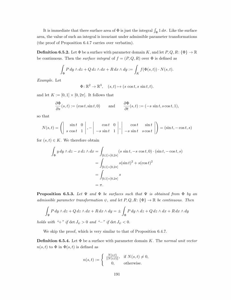
It is immediate that there surface area of Φ is just the integral∫
Φ 1 dσ. Like the surface
area, the value of such an integral is invariant under admissible parameter transformations
(the proof of Proposition 6.4.7 carries over verbatim).
Definition 6.5.2. Let Φ be a surface with parameter domainK, and let P,Q,R : {Φ} → Rbe continuous. Then the surface integral of f = (P,Q,R) over Φ is defined as∫
ΦP dy ∧ dz +Qdz ∧ dx+Rdx ∧ dy :=
∫Kf(Φ(s, t)) ·N(s, t).
Example. Let
Φ: R2 → R3, (s, t) 7→ (s cos t, s sin t, t).
and let K := [0, 1]× [0, 2π]. It follows that
∂Φ
∂s(s, t) := (cos t, sin t, 0) and
∂Φ
∂t(s, t) := (−s sin t, s cos t, 1),
so that
N(s, t) =
(∣∣∣∣∣ sin t 0
s cos t 1
∣∣∣∣∣ ,−∣∣∣∣∣ cos t 0
−s sin t 1
∣∣∣∣∣ ,∣∣∣∣∣ cos t sin t
−s sin t s cos t
∣∣∣∣∣)
= (sin t,− cos t, s)
for (s, t) ∈ K. We therefore obtain∫Φy dy ∧ dz − x dz ∧ dx =
∫[0,1]×[0,2π]
(s sin t,−s cos t, 0) · (sin t,− cos t, s)
=
∫[0,1]×[0,2π]
s(sin t)2 + s(cos t)2
=
∫[0,1]×[0,2π]
s
= π.
Proposition 6.5.3. Let Ψ and Φ be surfaces such that Ψ is obtained from Φ by an
admissible parameter transformation ψ, and let P,Q,R : {Φ} → R be continuous. Then∫ΨP dy ∧ dz +Qdz ∧ dx+Rdx ∧ dy = ±
∫ΦP dy ∧ dz +Qdz ∧ dx+Rdx ∧ dy
holds with “+” if det Jψ > 0 and “−” if det Jψ < 0.
We skip the proof, which is very similar to that of Proposition 6.4.7.
Definition 6.5.4. Let Φ be a surface with parameter domain K. The normal unit vector
n(s, t) to Φ in Φ(s, t) is defined as
n(s, t) :=
{N(s,t)‖N(s,t)‖ , if N(s, t) 6= 0,
0, otherwise.
191
Let Φ be a surface (with parameter domain K), and let f = (P,Q,R) : {Φ} → R3 be
continuous. Then we obtain∫ΦP dy ∧ dz +Qdz ∧ dx+Rdx ∧ dy =
∫Kf(Φ(s, t)) ·N(s, t)
=
∫Kf(Φ(s, t)) · n(s, t)‖N(s, t)‖
=
∫Φf · ndσ.
Theorem 6.5.5 (Stokes’ Theorem). Suppose that the following hypotheses are given:
(a) Φ is a C2-surface of which the parameter domain K is a normal domain (with respect
to both axes);
(b) the positively oriented boundary ∂K of K is parametrized by a piecewise C1-curve
γ : [a, b]→ R2;
(c) P , Q, and R are C1-functions defined on an open set containing {Φ}.
Then ∫Φ◦γ
P dx+Qdy +Rdz
=
∫Φ
(∂R
∂y− ∂Q
∂z
)dy ∧ dz +
(∂P
∂z− ∂R
∂x
)dz ∧ dx+
(∂Q
∂x− ∂P
∂y
)dx ∧ dy
=
∫Φ
(curl f) · ndσ
holds where f = (P,Q,R).
Remark. If {Φ} lies in the xy-plane, we recover (with additional hypotheses, of course)
Green’s Theorem.
Proof. Let Φ = (X,Y, Z), and
p(s, t) := P (X(s, t), Y (s, t), Z(s, t)).
We obtain ∫Φ◦γ
P dx =
∫ b
ap(γ(τ))
d(X ◦ γ)
dτ(τ) dτ
=
∫ b
ap(γ(τ))
(∂X
∂s(γ(τ))γ′1(τ) +
∂X
∂t(γ(τ))γ′2(τ)
)dτ
=
∫γp∂X
∂sds+ p
∂X
∂tdt.
192

By Green’s Theorem we have∫γp∂X
∂sds+ p
∂X
∂tdt =
∫K
(∂
∂s
(p∂X
∂t
)− ∂
∂t
(p∂X
∂s
)). (6.9)
We now transform the integral on the right hand side of (6.9). First note that
∂
∂s
(p∂X
∂t
)− ∂
∂t
(p∂X
∂s
)=∂p
∂s
∂X
∂t+ p
∂2X
∂s∂t− ∂p
∂t
∂X
∂s− p ∂
2X
∂t∂s=∂p
∂s
∂X
∂t− ∂p
∂t
∂X
∂s.
Furthermore, the Chain Rule yields that
∂p
∂s=∂P
∂x
∂X
∂s+∂P
∂y
∂Y
∂s+∂P
∂z
∂Z
∂s
and
∂p
∂t=∂P
∂x
∂X
∂t+∂P
∂y
∂Y
∂t+∂P
∂z
∂Z
∂t.
Combining all this, we obtain
∂p
∂s
∂X
∂t− ∂p
∂t
∂X
∂s
=
(∂P
∂x
∂X
∂s+∂P
∂y
∂Y
∂s+∂P
∂z
∂Z
∂s
)∂X
∂t−(∂P
∂x
∂X
∂t+∂P
∂y
∂Y
∂t+∂P
∂z
∂Z
∂t
)∂X
∂s
=∂P
∂y
(∂Y
∂s
∂X
∂t− ∂Y
∂t
∂X
∂s
)+∂P
∂z
(∂Z
∂s
∂X
∂t− ∂Z
∂t
∂X
∂s
)= −∂P
∂y
∣∣∣∣∣ ∂X∂s
∂X∂t
∂Y∂s
∂Y∂t
∣∣∣∣∣+∂P
∂z
∣∣∣∣∣ ∂Z∂s
∂Z∂t
∂X∂s
∂X∂t
∣∣∣∣∣ ,and therefore
∂
∂s
(p∂X
∂t
)− ∂
∂t
(p∂X
∂s
)= −∂P
∂y
∣∣∣∣∣ ∂X∂s
∂X∂t
∂Y∂s
∂Y∂t
∣∣∣∣∣+∂P
∂z
∣∣∣∣∣ ∂Z∂s
∂Z∂t
∂X∂s
∂X∂t
∣∣∣∣∣ .In view of (6.9), we thus have∫
Φ◦γP dx =
∫γp∂X
∂sds+ p
∂X
∂tdt
=
∫K
(−∂P∂y
∣∣∣∣∣ ∂X∂s
∂X∂t
∂Y∂s
∂Y∂t
∣∣∣∣∣+∂P
∂z
∣∣∣∣∣ ∂Z∂s
∂Z∂t
∂X∂s
∂X∂t
∣∣∣∣∣)
=
∫Φ−∂P∂y
dx ∧ dy +∂P
∂zdz ∧ dx. (6.10)
In a similar vein, we obtain∫Φ◦γ
Qdy =
∫Φ−∂Q∂z
dy ∧ dz +∂Q
∂xdx ∧ dy (6.11)
193

and ∫Φ◦γ
Rdz =
∫Φ−∂R∂x
dz ∧ dx+∂R
∂ydy ∧ dz. (6.12)
Adding (6.10), (6.11), and (6.12) completes the proof.
Example. Let γ be a counterclockwise parametrization of the circle {(x, y, z) ∈ R3 :
x2 + z2 = 1, y = 0}, and let
f(x, y, z) :=(x2z +
√x3 + x2 + 2︸ ︷︷ ︸=:P
, xy︸︷︷︸=:Q
, xy +√z3 + z2 + 2︸ ︷︷ ︸=:R
).
We want to compute ∫γP dx+Qdy +Rdz.
Let Φ be a surface with surface element {(x, y, z) ∈ R3 : x2 + z2 ≤ 1, y = 0}, e.g.,
Φ(s, t) := (s cos t, 0, s sin t)
for s ∈ [0, 1] and t ∈ [0, 2π]. It follows that
∂Φ
∂s(s, t) = (cos t, 0, sin t) and
∂Φ
∂t(s, t) = (−s sin t, 0, s cos t)
and thus
N(s, t) = (0,−s, 0)
for (s, t) ∈ K := [0, 1]× [0, 2π], so that
n(s, t) = (0,−1, 0)
for s ∈ (0, 1] and t ∈ [0, 2π]. It follows that
(curl f)(Φ(s, t)) · n(s, t) = −
(∂P
∂z(Φ(s, t))− ∂R
∂x(Φ(s, t))︸ ︷︷ ︸
=0
)= −s2(cos t)2
for s ∈ (0, 1] and t ∈ [0, 2π]. From Stokes’ Theorem, we obtain∫γP dx+Qdy +Rdz =
∫Φ
(curl f) · ndσ
=
∫K−s2(cos t)2s
= −(∫ 1
0s3 ds
)(∫ 2π
0(cos t)2 dt
)= −π
4.
194
Remark. Stokes’ Theorem allows for a physical interpretation of the curl of a vector field.
Let f be a continuously partially differentiable three-dimensional vector field that
models the velocity of a fluid, and let γ be a closed rectifiable curve. Then circulation
of f around γ given by∫γ f · d(x, y, z) is a measurement for the tendency of the fluid to
move around γ. Fix any point (x0, y0, z0) in the fluid and let Dr with r > 0 be a closed,
two-dimensional disc in the fluid, centered at (x0, y0, z0) with radius r. As the partial
derivatives of f are continuous, we obtain for r > 0 sufficiently small that
(curl f)(x, y, z) ≈ (curl f)(x0, y0, z0)
for all (x, y, z) ∈ Dr. Stoke’s Theorem then yields∫∂Dr
f · d(x, y, z) =
∫Dr
(curl f) · ndσ
≈∫Dr
(curl f)(x0, y0, z0) · n(x0, y0, z0) dσ
= πr2 (curl f)(x0, y0, z0) · n(x0, y0, z0),
so that
(curl f)(x0, y0, z0) · n(x0, y0, z0) = limr→0
1
πr2
∫∂Dr
f · d(x, y, z).
Hence, (curl f) · n can be thought of as a measurement for the rotating effect about the
axis given by n; it is largest when n and curl f are parallel.
Exercises
1. Let S be the upper hemisphere of the unit sphere in R3 (parametrized in the usual
way), and let
f(x, y, z) := (1, xz, xy)
for (x, y, z) ∈ R3. Use Stoke’s Theorem to compute∫S
(curl f) · ndσ.
2. Let Φ and Ψ be C2-surfaces with parameter domain K, which is a normal region,
such that Φ|∂K = Ψ|∂K , and let f : V → R3 be continuously differentiable where
V ⊂ R3 is open and contains {Φ} ∪ {Ψ}. Show that∫Φ
curl f · ndσ =
∫Ψ
curl f · ndσ.
195

6.6 Gauß’ Theorem
Suppose that a fluid is flowing through a certain part of three dimensional space. At each
point (x, y, z) in that part of space, suppose that a particle in that fluid has the velocity
v(x, y, z) ∈ R3 (independent of time; this is called a stationary flow). Suppose that the
fluid has the density ρ(x, y, z) at the point (x, y, z). The vector
f(x, y, z, t) := ρ(x, y, z, t)v(x, y, z)
is the density of the flow at (x, y, z).
Let S be a surface placed in the flow, and suppose that N 6= 0 throughout on S. Then
the mass passing through S in the direction of n is computed as∫Sf · ndσ. (6.13)
Fix a point (x0, y0, z0), and let
f = P i+Q j +Rk.
Let (x0, y0, z0) be the lower left corner of a box with sidelengths ∆x, ∆y, and ∆z.
∆x
∆y
x( y z )
z
y
x
∆z
0, 0, 0
Figure 6.14: Fluid streaming through a box
The mass passing through the two sides of the box parallel to the yz-plane is approx-
imately given by
P (x0, y0, z0) ∆y∆z and P (x0 + ∆x, y0, z0) ∆y∆z.
As an approximation for the mass flowing out of the box in the direction of the positive
x-axis, we therefore obtain
(P (x0 + ∆x, y0, z0)− P (x0, y0, z0)) ∆y∆z
=P (x0 + ∆x, y0, z0)− P (x0, y0, z0)
∆x∆x∆y∆z ≈ ∂P
∂x(x0, y0, z0) ∆x∆y∆z.
196
Similar considerations can be made for the y- and the z-axis. We thus have
mass flowing out of the box ≈(∂P
∂x+∂Q
∂y+∂R
∂z
)∆x∆y∆z = (div f) ∆x∆y∆z.
If V is a three-dimensional shape in the flow, we thus have
mass flowing out of V =
∫V
div f. (6.14)
If V has the surface S, (6.13) and (6.14), yield Gauß’s Theorem, namely∫Sf · ndσ =
∫V
div f
Of course, this is a far cry from a mathematically acceptable argument. To prove
Gauß’ theorem rigorously, we first have to define the domains in R3 over which we shall
be integrating:
Definition 6.6.1. Let U1, U2 ⊂ R2 be open, and let Φ1 ∈ C1(U1,R3) and Φ2 ∈ C1(U2,R3)
be surfaces with parameter domains K1 and K2, respectively, and write
Φν(s, t) = Xν(s, t) i+ Yν(s, t) j + Zν(s, t)k
for ν = 1, 2 and (s, t) ∈ Uν . Suppose that the following hold:
(a) the functions
gν : Uν → R2, (s, t) 7→ Xν(s, t) i+ Yν(s, t) j
for ν = 1, 2 are injective and satisfy det Jg1 < 0 and det Jg2 > 0 on K1 and K2,
respectively (except on a set of content zero);
(b) g1(K1) = g2(K2) =: K;
(c) the boundary of K is parametrized by a piecewise C1-curve;
(d) there are continuous functions φ1, φ2 : K → R with φ1 ≤ φ2 such that
Zν(s, t) = φν(Xν(s, t), Yν(s, t))
for ν = 1, 2 and (s, t) ∈ Kν .
Then
V := {(x, y, z) ∈ R3 : (x, y) ∈ K, φ1(x, y) ≤ z ≤ φ2(x, y)}
is called a normal domain with respect to the xy-plane. The surfaces Φ1 and Φ2 are called
the generating surfaces of V ; S1 := {Φ1} is called the lower lid, and S2 := {Φ2} the upper
lid of V .
197
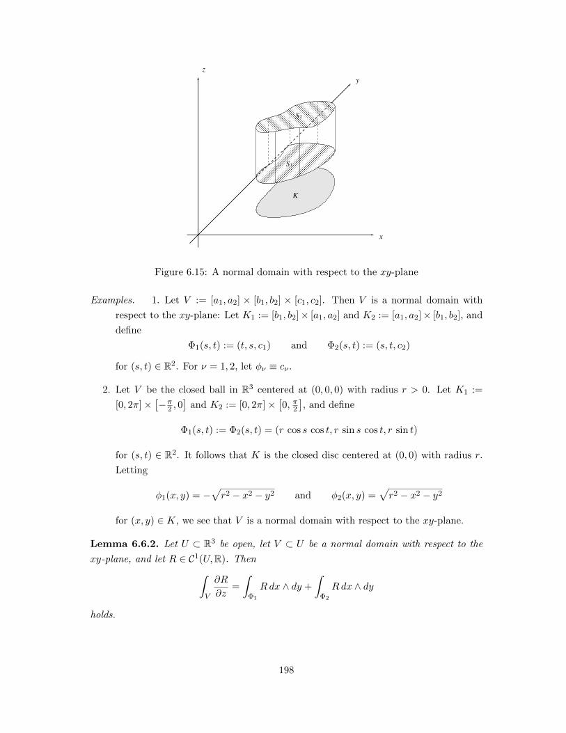
������������������������������������������������������������������������������������������������������������������������������������������������������������������������������������
������������������������������������������������������������������������������������������������������������������������������������������������������������������������������������
������������������������������������������������������������������������������������������������������������������������������������������������������������������
������������������������������������������������������������������������������������������������������������������������������������������������������������������
y
x
z
�����������
�����������
S2
S1
K
Figure 6.15: A normal domain with respect to the xy-plane
Examples. 1. Let V := [a1, a2] × [b1, b2] × [c1, c2]. Then V is a normal domain with
respect to the xy-plane: Let K1 := [b1, b2]× [a1, a2] and K2 := [a1, a2]× [b1, b2], and
define
Φ1(s, t) := (t, s, c1) and Φ2(s, t) := (s, t, c2)
for (s, t) ∈ R2. For ν = 1, 2, let φν ≡ cν .
2. Let V be the closed ball in R3 centered at (0, 0, 0) with radius r > 0. Let K1 :=
[0, 2π]×[−π
2 , 0]
and K2 := [0, 2π]×[0, π2
], and define
Φ1(s, t) := Φ2(s, t) = (r cos s cos t, r sin s cos t, r sin t)
for (s, t) ∈ R2. It follows that K is the closed disc centered at (0, 0) with radius r.
Letting
φ1(x, y) = −√r2 − x2 − y2 and φ2(x, y) =
√r2 − x2 − y2
for (x, y) ∈ K, we see that V is a normal domain with respect to the xy-plane.
Lemma 6.6.2. Let U ⊂ R3 be open, let V ⊂ U be a normal domain with respect to the
xy-plane, and let R ∈ C1(U,R). Then∫V
∂R
∂z=
∫Φ1
Rdx ∧ dy +
∫Φ2
Rdx ∧ dy
holds.
198

Proof. First note that∫V
∂R
∂z=
∫K
(∫ φ2(x,y)
φ1(x,y)
∂R
∂zdz
)=
∫K
(R(x, y, φ2(x, y))−R(x, y, φ1(x, y))).
Furthermore, we have∫KR(x, y, φ2(x, y)) =
∫g2(K2)
R(x, y, φ2(x, y))
=
∫K2
R(g2(s, t), φ2(g2(s, t))) detJg2(s, t)
=
∫K2
R(Φ2(s, t))
∣∣∣∣∣ ∂X2∂s (s, t) ∂X2
∂t (s, t)∂Y2∂s (s, t) ∂Y2
∂t (s, t)
∣∣∣∣∣=
∫K2
(0, 0, R(Φ2(s, t))) ·N(s, t)
=
∫Φ2
Rdx ∧ dy.
In a similar vein, we obtain∫KR(x, y, φ1(x, y)) = −
∫Φ1
Rdx ∧ dy.
All in all,∫V
∂R
∂z=
∫K
(R(x, y, φ2(x, y))−R(x, y, φ1(x, y))) =
∫Φ1
Rdx ∧ dy +
∫Φ2
Rdx ∧ dy
holds as claimed.
Let V ⊂ R3 be a normal domain with respect to the xy-plane, and let γ : [a, b] → R2
be a piecewise C1-curve that parametrizes ∂K. Let
K3 := {(s, t) ∈ R2 : s ∈ [a, b], φ1(γ(s)) ≤ t ≤ φ2(γ(s))}
and
Φ3(s, t) := γ1(s) i+ γ2(s) j + tk =: X3(s, t) i+ Y3(s, t) j + Z3(s, t)k
for (s, t) ∈ K3. Then Φ3 is a “generalized surface” whose surface element S3 := {Φ3} is
the vertical boundary of V .
Except for the points (s, t) ∈ K3 such that γ is not C1 at s—which is a set of content
zero—we have ∣∣∣∣∣ ∂X3∂s (s, t) ∂X3
∂t (s, t)∂Y3∂s (s, t) ∂Y3
∂t (s, t)
∣∣∣∣∣ =
∣∣∣∣∣ γ′1(s) 0
γ′2(s) 0
∣∣∣∣∣ = 0.
It therefore makes sense to define ∫Φ3
Rdx ∧ dy := 0.
199

Letting S := S1 ∪ S2 ∪ S3 = ∂V , we define∫SRdx ∧ dy :=
3∑ν=1
∫Φν
Rdx ∧ dy.
In view of Lemma 6.6.2, we obtain:
Corollary 6.6.3. Let U ⊂ R3 be open, let V ⊂ U be a normal domain with respect to the
xy-plane with boundary S, and let R ∈ C1(U,R). Then∫V
∂R
∂z=
∫SRdx ∧ dy
holds.
Normal domains in R3 can, of course, be defined with respect to all coordinate planes.
If a subset of R3 is a normal domain with respect to all coordinate planes, we simply
speak of a normal domain.
Theorem 6.6.4 (Gauß’ Theorem). Let U ⊂ R3 be open, let V ⊂ U be a normal domain
with boundary S, and let f ∈ C1(U,R3). Then∫Sf · ndσ =
∫V
div f
holds.
Proof. Let f = P i+Q j +Rk. By Corollary 6.6.3, we have∫SRdx ∧ dy =
∫V
∂R
∂z. (6.15)
Analogous considerations yield ∫SQdz ∧ dx =
∫V
∂Q
∂y(6.16)
and ∫SP dy ∧ dz =
∫V
∂P
∂x. (6.17)
Adding (6.15), (6.16), and (6.17), we obtain∫Sf · ndσ =
∫SP dy ∧ dz +Qdz ∧ dx+Rdx ∧ dy
=
∫V
∂P
∂x+∂Q
∂y+∂R
∂z
=
∫V
div f.
This proves Gauß’ Theorem.
200

Examples. 1. Let
V =
{(x, y, z) ∈ R3 : x2 + y2 + z2 ≤ 49
πe
},
and let
f(x, y, z) :=
(arctan(yz) + esin y, log(2 + cos(xz)),
1
1 + x2y2
).
Then Gauß’ Theorem yields that∫Sf · ndσ =
∫V
div f =
∫V
0 = 0.
2. Let S be the closed unit sphere in R3. Then∫S
2xy dy ∧ dz − y2 dz ∧ dx+ z3 dx ∧ dy =
∫S
(2xy,−y2, z3) · n(x, y, z) dσ
is difficult—if not impossible—to compute just using the definition of a surface
integral. With Gauß’ Theorem, however, the task becomes relatively easy. Let
f(x, y, z) := (2xy,−y2, z3)
for (x, y, z) ∈ R3, so that
(div f)(x, y, z) = 2y − 2y + 3z2 = 3z2.
By Gauß’ theorem, we have∫Sf · ndσ =
∫V
div f = 3
∫Vz2,
where V is the closed unit ball in R3. Passing to spherical coordinates and applying
Fubini’s theorem, we obtain∫Vz2 =
∫[0,1]×[0,2π]×[−π2 ,
π2 ]r4(sinσ)2(cosσ)
= 2π
∫ 1
0
(r4
∫ π2
−π2
(sinσ)2(cosσ) dσ
)dr
= 2π
∫ 1
0r4
(∫ 1
−1u2 du
)dr
= 2π
∫ 1
0
2
3r4 dr
=4π
15.
It follows that ∫Sf · ndσ =
∫V
div f = 3
∫Vz2 =
4π
5.
201

Exercises
1. Let S be the surface of the ball centered at (0, 0, 0) with radius r > 0. Compute∫Sx3 dy ∧ dz + y3 dz ∧ dx+ z3 dx ∧ dy.
2. Let V be the closed unit ball in R3, and let S := ∂V . Compute∫S
(2xy,−y2, z3) · n(x, y, z) dσ,
where n is the outward pointing unit normal vector on S, and dσ denotes integration
with respect to surface area.
3. Let V be a normal domain with boundary S such that N 6= 0 on S throughout, and
let f and g be R-valued C2-functions on an open set containing V .
(a) Prove Green’s First Formula:∫V
(∇f) · (∇g) +
∫Vf∆g =
∫SfDng dσ.
(b) Prove Green’s Second Formula:∫V
(f∆g − g∆f) =
∫S
(fDng − gDnf) dσ.
(Hint for (a): Apply Gauß’ Theorem to the vector field f∇g.)
4. Let ∅ 6= U ⊂ R3 be open, and suppose that f ∈ C2(U,R) is harmonic, i.e., satisfies
∆f = 0. Let V ⊂ U , S and n be as in the previous problem. Show that∫SDnf dσ = 0 and
∫SfDnf dσ =
∫V‖∇f‖2.
202
Chapter 7
Stokes’ Theorem for Differential
Forms
7.1 Alternating Multilinear Forms
Definition 7.1.1. Let r ∈ N. A map ω : (RN )r → R is called an r-linear form if, for each
j = 1, . . . , r, and all x1, . . . , xj−1, xj+1, . . . , xr ∈ RN , the map
R→ R, x 7→ ω(x1, . . . , xj−1, x, xj+1, . . . , xr)
is linear.
Example. Let ω1, . . . , ωr : RN → R be linear. Then
(RN )r → R, (x1, . . . , xr) 7→ ω1(x1) · · ·ωr(xr)
is an r-linear form.
Definition 7.1.2. Let r ∈ N. An r-linear form ω : (RN )r → R is called alternating if
ω(x1, . . . , xj , . . . , xk, . . . , xr) = −ω(x1, . . . , xk, . . . , xj , . . . , xr)
holds for all x1, . . . , xr ∈ RN and 1 ≤ j < k ≤ N .
We note the following:
1. If r = 1, then every linear map from RN to R is alternating.
2. If r > N , then zero is the only alternating, r-linear form.
3. If we identify MN (R) with (RN )N , then det is an alternating, N -linear form.
Definition 7.1.3. Let r ∈ N. Then Sr denotes the collection of all permutations of
{1, . . . , r}, i.e., the set of all bijective maps from {1, . . . , r} into itself.
203

Remarks. 1. The set Sr is a group under composition of maps.
2. A permutation of {1, . . . , r} is called a transposition if there are j < k such that
τ(j) = k, τ(k) = j and τ(l) = l for l ∈ {1, . . . , r} \ {j, k}.
Proposition 7.1.4. Let r ∈ N, and let σ ∈ Sr. Then there are transpositions τ1, . . . , τn ∈Sr such that σ = τ1 ◦ · · · ◦ τn.
Proof. We use induction on r.
The case r = 1 is clear: in this case, the identity is the only element of Sr, which is
a—empty—product of transpositions.
Suppose that the claim is true for all elements of Sr, and let σ ∈ Sr+1.
Case 1: σ(r + 1) = r + 1.
Then σ({1, . . . , r}) ⊂ {1, . . . , r}, so that σ|{1,...,r} ∈ Sr. By the induction hypothesis,
there are τ1, . . . , τn ∈ Sr such that σ|{1,...,r} = τ1◦· · ·◦τn. Define transpositions τ1, . . . , τn ∈Sr+1 by letting τj |{1,...,r} = τj and τj(r + 1) = r + 1 for j = 1, . . . , n. It is then clear that
σ = τ1 ◦ · · · ◦ τn.
Case 2: σ(r + 1) 6= r + 1.
Let τ ∈ Sr+1 be such that τ(σ(r+1)) = r+1, τ(r+1) = σ(r+1), and τ(k) = k for k ∈{1, . . . , r, r+1}\{r+1, σ(r+1)}. It follows that τ ◦σ ∈ Sr+1 with (τ ◦σ)(r+1) = r+1. By
Case 1, this means that there are transpositions τ1, . . . , τn ∈ Sr+1 with τ ◦σ = τ1 ◦· · ·◦τn,
so that σ = τ−1 ◦ τ1 ◦ · · · ◦ τn.
Definition 7.1.5. Let r ∈ N. Then the sign of σ ∈ Sr is defined as
sgnσ :=∏
1≤j<k≤r
σ(k)− σ(j)
k − j.
Proposition 7.1.6. Let r ∈ N. Then:
(i) sgnσ ∈ {−1, 1} for all σ ∈ Sr;
(ii) sgn : Sr → {−1, 1} is a group homomorphism where {−1, 1} is equipped with multi-
plication;
(iii) if ω is an alternating, r-linear form, then
ω(xσ(1), . . . , xσ(r)) = (sgnσ)ω(x1, . . . , xr)
for all σ ∈ Sr and x1, . . . , xr ∈ RN .
204

Proof. For (i) note that
sgnσ =∏
1≤j<k≤r
σ(k)− σ(j)
k − j
=∏
1≤j<k≤rσ(j)<σ(k)
σ(k)− σ(j)
k − j∏
1≤j<k≤rσ(j)>σ(k)
σ(k)− σ(j)
k − j
=∏
1≤j<k≤rσ(j)<σ(k)
(σ(k)− σ(j))∏
1≤j<k≤rσ(j)<σ(k)
1
k − j∏
1≤j<k≤rσ(j)>σ(k)
(σ(k)− σ(j))∏
1≤j<k≤rσ(j)>σ(k)
1
k − j
=∏
1≤j<k≤rσ(j)<σ(k)
(k − j)∏
1≤j<k≤rσ(j)<σ(k)
1
k − j
︸ ︷︷ ︸=1
∏1≤j<k≤rσ(j)>σ(k)
(j − k)∏
1≤j<k≤rσ(j)>σ(k)
1
k − j
︸ ︷︷ ︸=(−1)n
= (−1)n
where n is the number of pairs (j, k) with 1 ≤ j < k ≤ N and σ(j) > σ(k).
To prove (ii), let σ, τ ∈ Sr, and note that
(sgn)(σ ◦ τ) =∏
1≤j<k≤r
σ(τ(k))− σ(τ(j))
k − j
=∏
1≤j<k≤r
σ(τ(k))− σ(τ(j))
τ(k)− τ(j)
∏1≤j<k≤r
τ(k)− τ(j)
k − j
=
∏1≤j<k≤r
σ(τ(k))− σ(τ(j))
τ(k)− τ(j)
(sgn τ).
Now, ∏1≤j<k≤r
σ(τ(k))− σ(τ(j))
τ(k)− τ(j)=
∏1≤j<k≤rτ(j)<τ(k)
σ(τ(k))− σ(τ(j))
τ(k)− τ(j)
∏1≤j<k≤rτ(j)>τ(k)
σ(τ(k))− σ(τ(j))
τ(k)− τ(j)
=∏
1≤j<k≤rτ(j)<τ(k)
σ(τ(k))− σ(τ(j))
τ(k)− τ(j)
∏1≤j<k≤rτ(j)>τ(k)
σ(τ(j))− σ(τ(k))
τ(j)− τ(k)
=∏
1≤j<k≤r
σ(k)− σ(j)
k − j
= sgnσ,
so that sgn(σ ◦ τ) = (sgnσ)(sgn τ) as claimed.
Finally, let ω be an alternating, r-linear form, and let σ ∈ Sr. If σ is a transposition,
Definition 7.1.2 immediately yields that
ω(xσ(1), . . . , xσ(r)) = −ω(x1, . . . , xr) = (sgnσ)ω(x1, . . . , xr)
205
for all x1, . . . , xr ∈ RN . Suppose that σ ∈ Sr is arbitrary. Then, by Proposition 7.1.4,
there are transpositions τ1, . . . , τn ∈ Sr such that σ = τ1 ◦ · · · ◦ τn. It follows that
ω(xσ(1), . . . , xσ(r)) = ω(x(τ1◦···◦τn)(1), . . . , x(τ1◦···◦τn)(n))
= ω(xτ1(τ2◦···◦τn)(1)), . . . , xτ1(τ2◦···◦τn)(n)))
= (sgn τ1)ω(x(τ2◦···◦τn)(1), . . . , x(τ2◦···◦τn)(n)))
...
= (sgn τ1) · · · (sgn τn)ω(x1, . . . , xr)
= (sgnσ)ω(x1, . . . , xr)
for all x1, . . . , xr ∈ RN , which proves (iii).
Example. Let ω1, . . . , ωr : RN → R be linear. Then
ω1 ∧ · · · ∧ ωr : (RN )r → R, (x1, . . . , xr) 7→∑σ∈Sr
(sgnσ)ω1(xσ(1)) · · ·ωr(xσ(r))
is obviously an r-linear form. We claim that it is alternating. To see this, let τ ∈ Sr, and
note that
(ω1 ∧ · · · ∧ ωr)(xτ(1), . . . , xτ(r)) =∑σ∈Sr
(sgnσ)ω1(xσ(τ(1))) · · ·ωr(xσ(τ(r)))
= (sgn τ)−1︸ ︷︷ ︸=sgn τ
∑σ∈Sr
sgn(σ ◦ τ)ω1(x(σ◦τ)(1)) · · ·ωr(x(σ◦τ)(r))
= (sgn τ)∑σ∈Sr
(sgnσ)ω1(xσ(1)) · · ·ωr(xσ(r))
= (sgn τ)(ω1 ∧ · · · ∧ ωr)(x1, . . . , xr)
for all x1, . . . , xr ∈ RN .
Definition 7.1.7. For r ∈ N0, let Λr(RN ) := R if r = 0, and
Λr(RN ) := {ω : (RN )r → R : ω is an alternating, r-linear form}
if r ≥ 1.
It is immediate that Λr(RN ) is a vector space over R for all r ∈ N0.
Theorem 7.1.8. For j = 1, . . . , N , let
e∗j : RN → R, (x1, . . . , xN ) 7→ xj .
Then, for r ∈ N,
{e∗j1 ∧ · · · ∧ e∗jr : 1 ≤ j1 < · · · < jr ≤ N} (7.1)
is a basis for Λr(RN ).
206
Proof. For j = 1, . . . , N , let ej the jth canonical unit vector of RN , i.e., the jth coordinate
of ej is one and all the others are zero.
Let ω ∈ Λr(RN ), and let x1, . . . , xr ∈ RN . For k = 1, . . . , r and j = 1, . . . , N , let
λk,j ∈ R be such that xk =∑N
j=1 λk,jej . It follows that
ω(x1, . . . , xr) = ω
N∑j=1
λ1,jej , . . . ,N∑j=1
λr,jej
=
N∑j1=1
· · ·N∑jr=1
λ1,j1 · · ·λr,jrω (ej1 , . . . , ejr)
=
N∑j1,...,jr=1
λ1,j1 · · ·λr,jrω (ej1 , . . . , ejr)
=N∑
j1,...,jr=1jν 6= jµ for ν 6= µ
λ1,j1 · · ·λr,jrω (ej1 , . . . , ejr)
=∑
1≤j1<···<jr≤N
∑σ∈Sr
λ1,jσ(1) · · ·λr,jσ(r)ω(ejσ(1) , . . . , ejσ(r)
)=
∑1≤j1<···<jr≤N
∑σ∈Sr
λ1,jσ(1) · · ·λr,jσ(r)(sgnσ)ω (ej1 , . . . , ejr)
=∑
1≤j1<···<jr≤N
∑σ∈Sr
λ1,jσ(1) · · ·λr,jσ(r)(sgnσ)ω (ej1 , . . . , ejr)
(e∗j1 ∧ · · · ∧ e∗jr) (ej1 , . . . , ejr)
=∑
1≤j1<···<jr≤Nω (ej1 , . . . , ejr)
∑σ∈Sr
λ1,jσ(1) · · ·λr,jσ(r)(sgnσ)
(e∗j1 ∧ · · · ∧ e∗jr) (ej1 , . . . , ejr)
=∑
1≤j1<···<jr≤Nω (ej1 , . . . , ejr)
∑σ∈Sr
λ1,jσ(1) · · ·λr,jσ(r)
(e∗j1 ∧ · · · ∧ e∗jr)(ejσ(1) , . . . , ejσ(r)
)=
∑1≤j1<···<jr≤N
ω (ej1 , . . . , ejr) (e∗j1 ∧ · · · ∧ e∗jr)(x1, . . . , xr)
Consequently, (7.1) spans Λr(RN ). It is easy to see that the elements of (7.1) are linearly
independent and therefore form a basis of Λr(RN ).
Corollary 7.1.9. For all r ∈ N0, we have dim Λr(RN ) =(Nr
).
Corollary 7.1.10. ΛN (RN ) = R det.
We now define the wedge product of alternating multilinear forms:
207

Definition 7.1.11. Let r, s ∈ N. The the wedge product of e∗j1 ∧ · · · ∧ e∗jr∈ Λr(RN ) and
e∗jr+1∧ · · · ∧ e∗jr+s ∈ Λs(RN ) in Λr+s(RN ) is defined via
((e∗j1 ∧ · · · ∧ e∗jr) ∧ (e∗jr+1
∧ · · · ∧ e∗jr+s))(x1, . . . , xr+s)
:=∑
1≤j1<···<jr+s≤N
∑σ∈Sr+s
(sgnσ)e∗jσ(1)(x1) · · · e∗jσ(r+s)(xr+s)
for x1, . . . , xr+s ∈ RN .
Given r, s ∈ N, ω ∈ Λr(RN ), and φ ∈ Λs(RN ), we can use Theorem 7.1.8 to define
ω ∧ φ ∈ Λr+s(RN ) by means of linearity.
We record:
Proposition 7.1.12. Let r, s, t ∈ N, let λ ∈ R, and let ω ∈ Λr(RN ), φ ∈ Λs(RN ), and
ψ ∈ Λt(RN ). Then:
(i) (ω ∧ φ) ∧ ψ = ω ∧ (φ ∧ ψ);
(ii) λ(ω ∧ φ) = (λω) ∧ φ = ω ∧ (λφ);
(iii) (ω + φ) ∧ ψ = ω ∧ ψ + φ ∧ ψ;
(iv) ω ∧ (φ+ ψ) = ω ∧ φ+ ω ∧ ψ;
(v) ω ∧ φ = (−1)rsφ ∧ ω.
The verification is routine.
Exercises
1. Argue that the number n in Proposition 7.1.4 can be chosen to be less than or equal
to r − 1.
7.2 Differential Forms
Let ∅ 6= U ⊂ RN be open, and let r, p ∈ N0. By Corollary 7.1.9, we can canonically
identify the vector spaces Λr(RN ) and R(Nr ). Hence, it makes sense to speak of p-times
continuously partially differentiable maps from U to Λr(RN ).
Definition 7.2.1. Let ∅ 6= U ⊂ RN be open, and let r, p ∈ N0. A differential r-form—or
short: r-form—of class Cp on U is a Cp-function from U to Λr(RN ). The space of all
r-forms of class Cp is denoted by Λr(Cp(U)).
Remarks. 1. A zero-form of class Cp is simply a Cp-function with values in R.
208
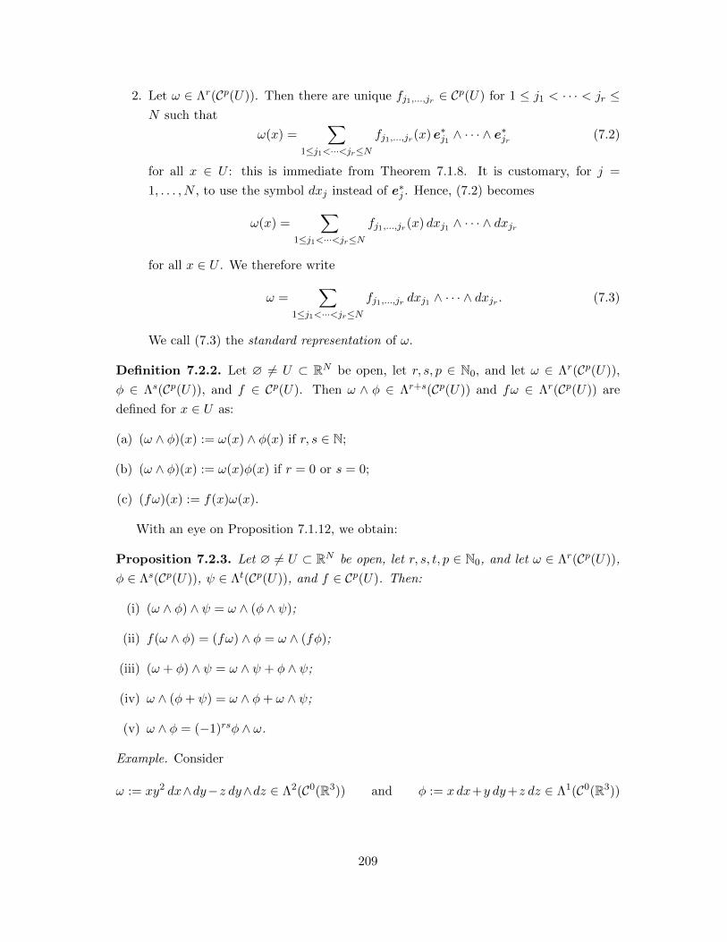
2. Let ω ∈ Λr(Cp(U)). Then there are unique fj1,...,jr ∈ Cp(U) for 1 ≤ j1 < · · · < jr ≤N such that
ω(x) =∑
1≤j1<···<jr≤Nfj1,...,jr(x) e∗j1 ∧ · · · ∧ e
∗jr (7.2)
for all x ∈ U : this is immediate from Theorem 7.1.8. It is customary, for j =
1, . . . , N , to use the symbol dxj instead of e∗j . Hence, (7.2) becomes
ω(x) =∑
1≤j1<···<jr≤Nfj1,...,jr(x) dxj1 ∧ · · · ∧ dxjr
for all x ∈ U . We therefore write
ω =∑
1≤j1<···<jr≤Nfj1,...,jr dxj1 ∧ · · · ∧ dxjr . (7.3)
We call (7.3) the standard representation of ω.
Definition 7.2.2. Let ∅ 6= U ⊂ RN be open, let r, s, p ∈ N0, and let ω ∈ Λr(Cp(U)),
φ ∈ Λs(Cp(U)), and f ∈ Cp(U). Then ω ∧ φ ∈ Λr+s(Cp(U)) and fω ∈ Λr(Cp(U)) are
defined for x ∈ U as:
(a) (ω ∧ φ)(x) := ω(x) ∧ φ(x) if r, s ∈ N;
(b) (ω ∧ φ)(x) := ω(x)φ(x) if r = 0 or s = 0;
(c) (fω)(x) := f(x)ω(x).
With an eye on Proposition 7.1.12, we obtain:
Proposition 7.2.3. Let ∅ 6= U ⊂ RN be open, let r, s, t, p ∈ N0, and let ω ∈ Λr(Cp(U)),
φ ∈ Λs(Cp(U)), ψ ∈ Λt(Cp(U)), and f ∈ Cp(U). Then:
(i) (ω ∧ φ) ∧ ψ = ω ∧ (φ ∧ ψ);
(ii) f(ω ∧ φ) = (fω) ∧ φ = ω ∧ (fφ);
(iii) (ω + φ) ∧ ψ = ω ∧ ψ + φ ∧ ψ;
(iv) ω ∧ (φ+ ψ) = ω ∧ φ+ ω ∧ ψ;
(v) ω ∧ φ = (−1)rsφ ∧ ω.
Example. Consider
ω := xy2 dx∧dy−z dy∧dz ∈ Λ2(C0(R3)) and φ := x dx+y dy+z dz ∈ Λ1(C0(R3))
209

In view of Proposition 7.2.3, we obtain for ω ∧ φ ∈ Λ3(C0(R3)) that
ω ∧ φ = x2y2 dx ∧ dy ∧ dx︸ ︷︷ ︸=0
+xy3 dx ∧ dy ∧ dy︸ ︷︷ ︸=0
+xy2z dx ∧ dy ∧ dz
− xz dy ∧ dz ∧ dx− yz dy ∧ dz ∧ dy︸ ︷︷ ︸=0
−z2 dy ∧ dz ∧ dz︸ ︷︷ ︸=0
= xy2z dx ∧ dy ∧ dz − xz dy ∧ dz ∧ dx
= (xy2z − xz) dx ∧ dy ∧ dz.
Definition 7.2.4. Let ∅ 6= U ⊂ RN be open. Then:
(a) the differential of f ∈ C1(U) is defined as
df :=
N∑j=1
∂f
∂xjdxj ∈ Λ1(C0(U));
(b) the outer differential of ω ∈ Λr(C1(U)) with r ∈ N in standard representation (7.3) is
defined as
dω :=∑
1≤j1<···<jr≤N
N∑j=1
∂fj1,...,jr∂xj
dxj ∧ dxj1 ∧ · · · ∧ dxjr ∈ Λr+1(C0(U)). (7.4)
Remark. In view of the properties of ∧, (7.4) is
dω =∑
1≤j1<···<jr≤Ndfj1,...,jr ∧ dxj1 ∧ · · · ∧ dxjr .
Examples. 1. Let ∅ 6= U ⊂ R2, and let ω := P dx+Qdy ∈ Λ1(C1(U)). Then
dω = dP ∧ dx+ dQ ∧ dy
=
(∂P
∂xdx+
∂P
∂ydy
)∧ dx+
(∂Q
∂xdx+
∂Q
∂ydy
)∧ dy
=∂P
∂ydy ∧ dx+
∂Q
∂xdx ∧ dy
=
(∂Q
∂x− ∂P
∂y
)dx ∧ dy.
210

2. Let ∅ 6= U ⊂ R3, and let ω := P dx+Qdy +Rdz ∈ Λ1(C1(U)). Then
dω = dP ∧ dx+ dQ ∧ dy + dR ∧ dz
=
(∂P
∂xdx+
∂P
∂ydy +
∂P
∂zdz
)∧ dx+
(∂Q
∂xdx+
∂Q
∂ydy +
∂Q
∂zdz
)∧ dy
+
(∂R
∂xdx+
∂R
∂ydy +
∂R
∂zdz
)∧ dz
=∂P
∂ydy ∧ dx+
∂P
∂zdz ∧ dx+
∂Q
∂xdx ∧ dy +
∂Q
∂zdz ∧ dy
+∂R
∂xdx ∧ dz +
∂R
∂ydy ∧ dz
=
(∂R
∂y− ∂Q
∂z
)dy ∧ dz +
(∂P
∂z− ∂R
∂x
)dz ∧ dx+
(∂Q
∂x− ∂P
∂y
)dx ∧ dy.
3. Let ∅ 6= U ⊂ R3, and let ω := P dy∧ dz+Qdz ∧ dx+Rdx∧ dy ∈ Λ2(C1(U)). Then
dω = dP ∧ dy ∧ dz + dQ ∧ dz ∧ dx+ dR ∧ dx ∧ dy
=
(∂P
∂xdx+
∂P
∂ydy +
∂P
∂zdz
)∧ dy ∧ dz
+
(∂Q
∂xdx+
∂Q
∂ydz ∧ dx+
∂Q
∂zdz
)∧ dz ∧ dx
+
(∂R
∂xdx+
∂R
∂ydy +
∂R
∂zdz
)dx ∧ dy
=∂P
∂xdx ∧ dy ∧ dz +
∂Q
∂ydy ∧ dz ∧ dx+
∂R
∂zdz ∧ dx ∧ dy
=
(∂P
∂x+∂Q
∂y+∂R
∂z
)dx ∧ dy ∧ dz.
The following holds:
Proposition 7.2.5. Let ∅ 6= U ⊂ RN be open, let r, s ∈ N0, let ω ∈ Λr(C1(U)) and
φ ∈ Λs(C1(U)), and let λ ∈ R. Then:
(i) d(ω + φ) = dω + dφ if r = s;
(ii) d(λω) = λdω;
(iii) d(ω ∧ φ) = dω ∧ φ+ (−1)rω ∧ dφ.
Proof. (i) and (ii) are routine.
For (iii), only consider the case where r, s ∈ N—the case where r = 0 or s = 0 is very
similar. In view of Proposition 7.2.3, we can suppose without loss of generality that
ω = f dxj1 ∧ · · · ∧ dxjr and φ = g dxk1 ∧ · · · ∧ dxks
211

with f, g ∈ C1(U) and 1 ≤ j1 < · · · < jr ≤ N and 1 ≤ k1 < · · · < ks ≤ N . It follows that
ω ∧ φ = fg dxj1 ∧ · · · ∧ dxjr︸ ︷︷ ︸=:α
∧ dxk1 ∧ · · · ∧ dxks︸ ︷︷ ︸=:β
,
so that
d(ω ∧ φ) = d(fg) ∧ α ∧ β
= g df ∧ α ∧ β + f dg ∧ α ∧ β, because d(fg) = g df + f dg,
= (df ∧ α) ∧ (gβ) + dg ∧ fα ∧ β
= (df ∧ α) ∧ (gβ) + (−1)r(fα) ∧ (dg ∧ β), by Proposition 7.2.3(v),
= dω ∧ φ+ (−1)rω ∧ dφ.
This proves the claim.
Theorem 7.2.6. Let ∅ 6= U ⊂ RN be open, let r ∈ N0, and let ω ∈ Λr(C2(U)). Then
d(dω) = 0.
Proof. Suppose first that r = 0, i.e., ω = f ∈ C2(U). Then
d(dω) = d
N∑j=1
∂f
∂xjdxj
=
N∑j=1
N∑k=1
∂2f
∂xk∂xjdxk ∧ dxj
=N∑
j,k=1j 6=k
∂2f
∂xk∂xjdxk ∧ dxj
=∑
1≤j<k≤N
(∂2f
∂xk∂xj− ∂2f
∂xj∂xk
)dxk ∧ dxj
= 0
by Clairaut’s Theorem.
Let r ∈ N. Without loss of generality, we can suppose that
ω = f dxj1 ∧ · · · ∧ dxjr︸ ︷︷ ︸=:α
with f ∈ C2(U) and 1 ≤ j < k ≤ N . From Proposition 7.2.5(iii), we conclude that
d(dω) = d(df ∧ α) = d(df) ∧ α− df ∧ dα.
As d(df) = 0 by the foregoing and dα = 0 for trivial reasons, we obtain d(dω) = 0.
212

Definition 7.2.7. Let ∅ 6= V ⊂ RM and ∅ 6= U ⊂ RN be open, let T = (t1, . . . , tN ) : V →U be of class C1, let r ∈ N0, and let ω ∈ Λr(C0(U)). Then the T -pullback ωT ∈ Λr(C0(V ))
of ω is defined as follows:
(a) if r = 0, i.e., ω = f ∈ C0(U), then ωT = fT = f ◦ T ;
(b) if r ∈ N and ω is in standard form (7.3), then
ωT :=∑
1≤j1<···<jr≤N(fj1,...,jr ◦ T ) dtj1 ∧ · · · ∧ dtr
where
dtj =M∑k=1
∂tj∂xk
dxk
for j = 1, . . . , N .
Proposition 7.2.8. Let ∅ 6= V ⊂ RM and ∅ 6= U ⊂ RN be open, let T = (t1, . . . , tN ) :
V → U be of class C1, let r, s ∈ N0, and let ω ∈ Λr(C0(U)) and φ ∈ Λs(C0(U)). Then:
(i) (ω + φ)T = ωT + φT if r = s;
(ii) (ω ∧ φ)T = ωT ∧ φT ;
(iii) dωT = (dω)T if ω ∈ Λr(C1(U)) and T ∈ C2(V,RN ).
Proof. (i) and (ii) are routine.
For (iii), suppose first that ω = f ∈ C1(U). Then
dfT =M∑j=1
∂(f ◦ T )
∂xjdxj
=
M∑j=1
(N∑k=1
(∂f
∂yk◦ T)∂tk∂xj
)dxj
=
N∑k=1
( ∂f
∂yk◦ T) M∑j=1
∂tk∂xj
dxj
=
N∑k=1
(∂f
∂yk◦ T)dtk
= (df)T ,
so that the claim is settled in this case.
For the case where r ∈ N, we suppose again that
ω = f dxj1 ∧ · · · ∧ dxjr︸ ︷︷ ︸=:α
213

with f ∈ C1(U) and 1 ≤ j < k ≤ N . We note that αT = dtj1 ∧ · · · ∧ dtjr and therefore
dαT = 0 by Exercise 7.2.5. It follows that
dωT = dfT ∧ αT + fT dαT = dfT ∧ αT = (df)T ∧ αT = (df ∧ α)T = (dω)T ,
which proves the claim.
Proposition 7.2.9. Let ∅ 6= W ⊂ RK , ∅ 6= V ⊂ RM , and ∅ 6= U ⊂ RN be open,
let T = (t1, . . . , tM ) : W → V and S = (s1, . . . , sN ) : V → U , let r ∈ N0, and let
ω ∈ Λr(C0(U)). Then (ωS)T = ωS◦T .
Proof. The claim is obvious for r = 0. For r ∈ N, we can suppose without loss of generality
that ω = dzj with j ∈ {1, . . . , N}: this follows from the standard representation (7.3) of
ω and Proposition 7.2.8. In this case, by definition,
(dzj)S = dsj =
M∑k=1
∂sj∂yk
dyk
and, consequently,
((dzj)S)T =M∑k=1
(∂sj∂yk◦ T)dtk
=
M∑k=1
(∂sj∂yk◦ T) K∑ν=1
∂tk∂xν
dxν
=K∑ν=1
(M∑k=1
(∂sj∂yk◦ T)∂tk∂xν
)dxν .
On the other hand, let u1, . . . , uN ∈ C1(W ) be the coordinate functions of S ◦ T . Then
(dzj)S◦T = duj
=
K∑ν=1
∂uj∂xν
dxν
=
K∑ν=1
(M∑k=1
(∂sj∂yk◦ T)∂tk∂xν
)dxν ,
so that ((dzj)S)T = (dzj)S◦T .
Exercises
1. Let
ω := sin(xy) dx+ exz dy − zx dz and φ := xyz dx ∧ dz + cos z dx ∧ dy.
Compute ω ∧ φ and d(ω ∧ φ), expressing both differential forms in their respective
standard representation.
214

2. Let ∅ 6= U ⊂ RN be open, and let f = (f1, . . . , fN ) ∈ C1(U,RN ). Show that
df1 ∧ · · · ∧ dfN = det Jf dx1 ∧ · · · ∧ dxN .
3. Let ∅ 6= U ⊂ RN be open, and let r ∈ N0. Then ω ∈ Λr(C1(U)) is called closed if
dω = 0. Show that:
(a) each ω ∈ ΛN (C1(U)) is closed;
(b) ω =∑N
j=1 fj dxj ∈ Λ1(C1(U)) is closed if and only if
∂fj∂xk
=∂fk∂xj
on U for all j, k = 1, . . . , N .
4. Let ∅ 6= U ⊂ R be open, let r, s ∈ N0, and let ω ∈ Λr(C1(U)) and φ ∈ Λs(C1(U)) be
closed. Show that ω ∧ φ is closed.
5. Let ∅ 6= U ⊂ RN be open, and let f1, . . . , fn ∈ C2(U). Show that df1 ∧ · · · ∧ dfn is
closed. (Hint : Induction on n.)
6. Let ∅ 6= U ⊂ RN be open, and let r ∈ N. Then ω ∈ Λr(C0(U)) is called exact if
there is φ ∈ Λr−1(C1(U)) such that ω = dφ. Show that:
(a) if ω ∈ Λr(C1(U)) is exact, then it is closed;
(b) if U is star shaped and ω ∈ Λ1(C1(U)) is closed, then ω is exact.
7.3 Integration of Differential Forms
Definition 7.3.1. Let U ⊂ Rr be open, and let ∅ 6= K ⊂ U be compact and with
content. An r-surface Φ of class Cp in RN with parameter domain K is the restriction of
a Cp-function Φ : U → RN to K. The set K is called the parameter domain of Φ, and
{Φ} := Φ(K) is called the trace or the surface element of Φ.
Definition 7.3.2. Let r ∈ N, let Φ = (φ1, . . . , φN ) be an r-surface of class C1 in RN with
parameter domain K, and let ω be an r-form of class C0 on a neighborhood of {Φ} with
a unique representation as in (7.3). Then the integral of ω over Φ is defined as
∫Φω :=
∑1≤j1<···<jr≤N
∫K
(fj1,...,jr ◦ Φ)
∣∣∣∣∣∣∣∣∂φj1∂x1
, . . . ,∂φj1∂xr
.... . .
...∂φjr∂x1
, . . . ,∂φjr∂xr
∣∣∣∣∣∣∣∣ .
215

Examples. 1. Let N be arbitrary, and let r = 1. Then ω is of the form
ω = f1 dx1 + · · ·+ fN dxN .
Let a < b, and let γ = (γ1, . . . , γN ) : [a, b] → RN be a C1-curve. Let ε > 0. For
j = 1, . . . , N , define
γ′j : (a− ε, b+ ε)→ R, t 7→
γj(a), a− ε < t ≤ a,γj(t), a ≤ t ≤ b,γj(b), b ≤ t < b+ ε.
Then γ′1, . . . , γ′N are continuous and extend γ′1, . . . , γ
′N . It follows that, for j =
1, . . . , N , the functions
γj : (a− ε, b+ ε)→ R, t 7→ γj(a) +
∫ t
aγ′j(s) ds
are of class C1 and extend γ1, . . . , γN , respectively. Set U := (a−ε, b+ε), K := [a, b],
and define
Φ: U → RN , t 7→ (γ1, . . . , γN ) .
Then Φ is a C1-curve γ, and∫Kω =
N∑j=1
∫ b
afj(γ(t))γ′1(t) dt =
∫γf1 dx1 + · · ·+ fN dxN ,
i.e., the curve integral of the vector field (f1, . . . , fN ) along the curve γ as described
in Theorem 6.2.4 is a special case of Definition 7.3.2.
2. Let N = 3, and let r = 2, i.e., Φ is a surface in the sense of Definition 6.4.1. The
normal vector to Φ at Φ(s, t) with (s, t) in the parameter domain K of Φ is
N(s, t)
=
(∣∣∣∣∣ ∂φ2∂s (s, t) ∂φ3
∂s (s, t)∂φ2∂t (s, t) ∂φ3
∂t (s, t)
∣∣∣∣∣ ,−∣∣∣∣∣ ∂φ1
∂s (s, t) ∂φ3∂s (s, t)
∂φ1∂t (s, t) ∂φ3
∂t (s, t)
∣∣∣∣∣ ,∣∣∣∣∣ ∂φ1
∂s (s, t) ∂φ2∂s (s, t)
∂φ1∂t (s, t) ∂φ2
∂t (s, t)
∣∣∣∣∣).
Given a continuous vector field f = (P,Q,R) defined on a neighborhood of {Φ} the
surface integral of f over Φ in the sense of Definition 6.5.2 is∫ΦP dy ∧ dz +Qdz ∧ dx+Rdx ∧ dy
=
∫K
(f ◦ Φ) ·N
=
∫K
(P ◦ Φ)
∣∣∣∣∣ ∂φ2∂s
∂φ3∂s
∂φ2∂t
∂φ3∂t
∣∣∣∣∣− (Q ◦ Φ)
∣∣∣∣∣ ∂φ1∂s
∂φ3∂s
∂φ1∂t
∂φ3∂t
∣∣∣∣∣+ (R ◦ Φ)
∣∣∣∣∣ ∂φ1∂s
∂φ3∂s
∂φ1∂t
∂φ3∂t
∣∣∣∣∣=
∫Φω
216

with the last integral being in the sense of Definition 7.3.2 where
ω := P dy ∧ dz −Qdx ∧ dz +Rdx ∧ dy = P dy ∧ dz +Qdz ∧ dx+Rdx ∧ dy.
So, the meanings assigned to the symbol∫ΦP dy ∧ dz +Qdz ∧ dx+Rdx ∧ dy
by Definitions 7.3.2 and 6.5.2 are identical.
The following is straightforward:
Lemma 7.3.3. Let Φ be an r-surface of class C1 with parameter domain K, and let ω1
and ω2 be r-forms of class C0 on an open neighborhood of {Φ}, and let λ1, λ2 ∈ R. Then∫Φλ1ω1 + λ2ω2 = λ1
∫Φω1 + λ2
∫Φω2.
Lemma 7.3.4. Let r ∈ N, let ∅ 6= U ⊂ RN be open, let ω ∈ Λr(C0(U)), Φ = (φ1, . . . , φN )
be an r-surface of class C1 in RN with parameter domain K such that {Φ} ⊂ U , and let
Ψ be the restriction of the identity map on Rr to K. Then∫Φω =
∫ΨωΦ.
Proof. In view of Lemma 7.3.3, we can limit ourselves to the case where
ω = f dxj1 ∧ · · · ∧ dxjr ,
with f ∈ C0(U) and 1 ≤ j1 < · · · < jr ≤ N , so that
ωΦ = (f ◦ Φ) dφj1 ∧ · · · ∧ dφjr
= (f ◦ Φ)
∣∣∣∣∣∣∣∣∂φj1∂x1
, . . . ,∂φj1∂xr
.... . .
...∂φjr∂x1
, . . . ,∂φjr∂xr
∣∣∣∣∣∣∣∣ dx1 ∧ · · · ∧ dxr
with the last equality being due to Exercise 7.2.2. Consequently, we obtain
∫ΨωΦ =
∫Ψ
(f ◦ Φ)
∣∣∣∣∣∣∣∣∂φj1∂x1
, . . . ,∂φj1∂xr
.... . .
...∂φjr∂x1
, . . . ,∂φjr∂xr
∣∣∣∣∣∣∣∣ dx1 ∧ · · · ∧ dxr
=
∫K
(f ◦ Φ)
∣∣∣∣∣∣∣∣∂φj1∂x1
, . . . ,∂φj1∂xr
.... . .
...∂φjr∂x1
, . . . ,∂φjr∂xr
∣∣∣∣∣∣∣∣ dx1 ∧ · · · ∧ dxr
=
∫Φω,
which proves the claim.
217
Theorem 7.3.5. Let ∅ 6= V ⊂ RM and ∅ 6= U ⊂ RN be open, let r ∈ N, let ω ∈Λr(C0(V )), let Φ be an r-surface of class C1 with {Φ} ⊂ V , and let T ∈ C1(V,RN ) with
T (V ) ⊂ U . Then ∫T◦Φ
ω =
∫ΦωT .
Proof. Let Ψ be as in Lemma 7.3.4, so that by that lemma∫T◦Φ
ω =
∫ΨωT◦Φ and
∫ΦωT =
∫Ψ
(ωT )Φ.
As (ωT )Φ by Proposition 7.2.9, this proves the claim.
7.4 Simplices and Chains
Definition 7.4.1. The unit simplex in RN is defined as
ΣN :=
(x1, . . . , xN ) ∈ RN : x1, . . . , xN ≥ 0,N∑j=1
xj ≤ 1
Examples. 1. Σ1 = [0, 1].
2. Σ2 is the triangle with vertices 0, i and j.
3. Σ3 is the tetrahedron with vertices 0, i, j, and k.
Definition 7.4.2. Let r ∈ N, and let (x0, x1, . . . , xr) ∈ (RN )r+1. Then the oriented affine
r-simplex [x0, x1, . . . , xr] is the r-surface in RN with parameter domain Σr given by
[x0, x1, . . . , xr] : Rr → RN , (t1, . . . , tr) 7→ x0 + t1(x1 − x0) + · · ·+ tr(xr − x0).
The points x0, x1, . . . , xr are called the vertices of [x0, x1, . . . , xr].
Remark. Note that the unit simplex in RN is not an oriented affine simplex in the sense
of Definition 7.4.2: the former is a set, the latter a (restriction of a) map.
Definition 7.4.3. Let r ∈ N. Then we call σ ∈ Sr even if sgnσ = 1 and odd if
sgnσ = −1.
Definition 7.4.4. Let (x0, x1, . . . , xr), (y0, y1, . . . , yr) ∈ RN . Then we call [x0, x1, . . . , xr]
and [y0, y1, . . . , yr] equivalent—in symbols: [x0, x1, . . . , xr] ∼ [y0, y1, . . . , yr]—if there is an
even σ ∈ Sr+1 such that yj = xσ(j) for j = 0, 1, . . . , r. We set
Jx0, x1, . . . , xrK := {[y0, y1, . . . , yr] : [x0, x1, . . . , xr] ∼ [y0, y1, . . . , yr]}
218
Remarks. 1. Definition 7.4.4 partitions {[xσ(0), xσ(1), . . . , xσ(r)] : σ ∈ Sr+1} into two
equivalence classes, namely Jx0, x1, . . . , xrK and
−Jx0, x1, . . . , xrK := {[xσ(0), xσ(1), . . . , xσ(r)] : σ ∈ Sr+1, σ odd}.
2. For convenience, if Σ = [x0, x1, . . . , xr], we write JΣK for Jx0, x1, . . . , xrK and −JΣKfor −Jx0, x1, . . . , xrK.
So far, oriented affine r-simplices were defined only for r ∈ N. For formal reasons, we
now define:
Definition 7.4.5. An oriented affine 0-simplex in RN is a pair (ε, x0) with ε ∈ {−1, 1}and x0 ∈ RN . We write
[x0] := (1, x0), −[x0] := (−1, x0), and Jx0K := [x0].
Definition 7.4.6. Let r ∈ N0. An affine r-chain in RN is a formal sum JΣ1K⊕· · ·⊕ JΣmKwhere Σ1, . . . ,Σm are oriented affine r-simplices in RN .
Remarks. 1. Somewhat abusing notation, we will also write JΣ1⊕· · ·⊕ΣmK for oriented
affine r-simplices Σ1, . . . ,Σm in RN or even Σ1 ⊕ · · · ⊕ Σm.
2. Given oriented affine r-simplices Σ1, . . . ,Σm in RN and ε1, . . . , εm ∈ {−1, 1}, we
convene that ε1Σ1 ⊕ · · · ⊕ εmΣm denotes ε1JΣ1K⊕ · · · ⊕ εmJΣmK.
Definition 7.4.7. Let r ∈ N, and let Σ := [x0, x1, . . . , xr] be an oriented affine r-simplex
in RN . Then the oriented boundary of Σ is defined as
∂Σ :=
r⊕j=0
(−1)r[x0, . . . , xj−1, xj+1, . . . , xr].
Remark. Obviously, ∂Σ is an affine r-chain.
Examples. 1. If Σ = [x0, x1], then ∂Σ = [x1]⊕ (−[x0]).
2. If Σ = [x0, x1, x2], then
∂Σ = [x1, x2]⊕ (−[x0, x2])⊕ [x0, x1] = [x0, x1]⊕ [x1, x2]⊕ [x2, x0].
Definition 7.4.8. Let r ∈ N. An oriented r-simplex in RN is an r-surface Φ of the form
T ◦ Σ such that:
(a) Σ is an oriented affine r-simplex in RM ;
(b) T is a C2-map defined on an open neighborhood of {Σ}.
219

Remarks. 1. If Φ1 and Φ2 are two oriented r-simplices of the form T ◦ Σ1 and T ◦ Σ2,
respectively, we define
Φ1 ∼ Φ2 :⇐⇒ Σ1 ∼ Σ2
and denote the corresponding equivalence class by JΦ1K.
2. As for oriented affine r-simplices, we have—given an oriented r-simplex Φ = T ◦Σ—
there are two equivalence classes denoted by JΦK and −JΦK.
3. We write T ◦ JΣK for JT ◦ ΣK: this is clearly well defined.
Definition 7.4.9. An oriented 0-simplex in RN is a pair (ε, T (x0)) with ε ∈ {−1, 1},x0 ∈ RM , and T is a C2-map into RN defined on a neighborhood of x0. We write
T ◦ [x0] := (1, x0), −T ◦ [x0] := (−1, x0), and JT ◦ x0K := T ◦ [x0].
Definition 7.4.10. Let r ∈ N0. An r-chain in RN is a formal sum JΦ1K ⊕ · · · ⊕ JΦmKwhere Φ1, . . . ,Φm are oriented r-simplices in RN of the form T ◦Σj for j = 1, . . . ,m where
Σ1, . . . ,Σm are oriented affine r-simplices in RM and T is a C2-map defined on an open
neighborhood of {Σ1} ∪ · · · ∪ {Σm}. The trace or surface element of JΦ1K⊕ · · · ⊕ JΦmK is
defined as
{JΦ1K⊕ · · · ⊕ JΦmK} := {Φ1} ∪ · · · ∪ {Φm}.
Remark. Given Φ1 = T ◦ Σ1 and Φ1 = T ◦ Σ1, we write JΦ1K = −JΦ2K if JΣ1K = −JΣ2K
Definition 7.4.11. Let r ∈ N. Then:
(a) if Φ is an oriented r-simplex Φ = T ◦ Σ in RN , the oriented boundary of Φ is defined
as the (r − 1)-chain
∂Φ :=
r⊕j=0
(−1)r T ◦ [x0, . . . , xj−1, xj+1, . . . , xr].
(b) if Φ1, . . . ,Φm are oriented r-simplices in RN , then the oriented boundary of Φ :=
Φ1 ⊕ · · · ⊕ Φm is defined as
∂Φ := ∂Φ1 ⊕ · · · ⊕ ∂Φm.
Remark. We convene that, whenever in an expression Φ1 ⊕ · · · ⊕ Φm, there are 1 ≤ j <
k ≤ m with Φk = −Φj , then Φj and Φk cancel each other.
Examples. 1. Let
x0 :=
[−π0
], x1 :=
[0
−π
], x2 :=
[π
0
], and x3 :=
[0
π
].
220
Set
Σ1 := [x0, x1, x2] and Σ2 := [x2, x3, x0],
so that
{Σ1 ⊕ Σ2} = {Σ1} ∪ {Σ2} = {(x, y) ∈ R2 : |x|+ |y| ≤ π}.
Let r > 0, and define
Tr : R2 → R2, (s, t)→ (r cos s, r sin t).
Set Φ1 := Tr ◦ Σ1, Φ2 := Tr ◦ Σ2, and Φr := Φ1 ⊕ Φ2. Then
{Φr} = {Φ1} ∪ {Φ2} = Br[(0, 0)]
and
∂Φr = Tr ◦ ∂Σ1 ⊕ Tr ◦ ∂Σ2
= Tr ◦ [x0, x1]⊕ Tr ◦ [x1, x2]⊕ Tr ◦ [x2, x0]
⊕ Tr ◦ [x2, x3]⊕ Tr ◦ [x3, x0]⊕ Tr ◦ [x0, x2]
= Tr ◦ [x0, x1]⊕ Tr ◦ [x1, x2]⊕ Tr ◦ [x2, x3]⊕ Tr ◦ [x3, x0],
i.e., ∂Φr is ∂Br[(0, 0)] in counterclockwise orientation.
2. Let 0 < r < R, and set Φ := ΦR ⊕ (−Φr). Then {Φ} = BR[(0, 0)] and
∂Φ = ∂ΦR ⊕ (−∂Φr),
i.e., ∂BR((0, 0)) in counterclockwise orientation “plus” ∂Br((0, 0)) in clockwise ori-
entation. This can be interpreted as the boundary of the annulus BR[(0, 0)]\Br(0, 0)
with the “outer” circle being oriented counterclockwise and the “inner” one being
oriented clockwise
221

R
r
Figure 7.1: Oriented boundary of BR[(0, 0)] \Br(0, 0)
We note:
Proposition 7.4.12. Let r ∈ N, let Σ = [x0, x1, . . . , xr] be an oriented affine r-simplex,
let σ ∈ Sr+1, and set Σσ := [xσ(0), xσ(1), . . . , xσ(r)]. Then, for any r-form ω of class C0
on an open neighborhood of {Σ} = {Σσ}, we have∫Σσ
ω = (sgnσ)
∫Σω. (7.5)
Proof. We can suppose without loss of generality that
ω = f dj1 ∧ · · · ∧ djr
for a continuous function f : {Σ} → R. Furthermore, in view of of Propositions 7.1.4 and
7.1.6(ii), it is enough to prove (7.5) in the case where σ is a transposition, in which case
(7.6) becomes ∫Σσ
ω = −∫
Σω. (7.6)
Suppose therefore that σ is a transposition.
Case 1: σ(0) = 0. Note that then
Σ(t1, . . . , tr) =
1−r∑j=1
x0 + t1x1 + · · ·+ trxr
and
Σσ(t1, . . . , tr) =
1−r∑j=1
x0 + t1xσ(1) + · · ·+ trxσ(r)
222

for (t1, . . . , tr) ∈ Rr. Define
Φ: Rr → Rr, (t1, . . . , tr) 7→ (tσ(1), . . . , tσ(r)),
so that
Φ(Σr) = Σr, Σ = Σσ ◦ Φ, and detJΦ = 1. (7.7)
Let Σσ,1, . . . ,Σσ,N denote the coordinate functions of Σσ. It is obvious that∣∣∣∣∣∣∣∣∂Σσ,j1∂x1
, . . . ,∂Σσ,j1∂xr
.... . .
...∂Σσ,jr∂x1
, . . . ,∂Σσ,jr∂xr
∣∣∣∣∣∣∣∣ = c
for some c ∈ R. From (7.5), we obtain therefore that
ωΣσ = c (f ◦ Σσ) dt1 ∧ · · · ∧ dtr.
Viewing Φ is an r-surface with parameter domain Σr, we eventually get∫σω =
∫Σσ◦Φ
ω
=
∫ΦωΣσ
= c
∫Φ
(f ◦ Σσ) dt1 ∧ · · · ∧ dtr
= c
∫Σr
(f ◦ Σσ ◦ Φ) det JΦ
= −c∫
Σr
f ◦ Σσ ◦ Φ | det JΦ|
= −c∫
Φ(Σr)f ◦ Σσ
= −∫
Σr
c (f ◦ Σσ)
= −∫
Σσ
ω,
which proves (7.6) in this case.
Case 2: σ(0) 6= 0.
Suppose first that σ(0) = 1. Define
Φ: Rr → Rr, (t1, . . . , tr) 7→
1−r∑j=1
tj , t2, . . . , tr
.
Then Φ also satisfies (7.7), and the same argument as in Case 2 proves (7.6). If σ(0) =
k /∈ {0, 1}, let τ ∈ Sr+1 be the permutation that interchanges k and 1. Then τ ◦ σ ◦ τ is
223

a transposition that interchanges 0 and 1, so that (7.6) holds with τ ◦ σ ◦ σ en lieu of σ.
On the other hand, τ(0) = 0, so that Case 1 applies to τ en lieu of σ. It follows that∫Σσ
ω =
∫Στ◦τ◦σ◦τ◦τ
ω =
∫((Στ )τ◦σ◦τ )τ
ω = −∫
(Στ )τ◦σ◦τ
ω =
∫Στ
ω = −∫
Σω,
so that (7.6) holds in this case, too.
In view of Lemma 7.3.4, we conclude:
Corollary 7.4.13. Let r ∈ N, let Σ = [x0, x1, . . . , xr] be an oriented affine r-simplex, let
σ ∈ Sr+1, and set Σσ := [xσ(0), xσ(1), . . . , xσ(r)]. Then, for any map T of class C2 defined
on an open neighborhood of {Σ} = {Σσ}, and for any r-form ω of class C0 on an open
neighborhood of {T ◦ Σ} = {T ◦ Σσ}, we have∫T◦Σσ
ω = (sgnσ)
∫T◦Σ
ω.
In Definition 7.3.2, we defined the integral of an r-form for r ∈ N. We now define it
for r = 0:
Definition 7.4.14. Let x0 ∈ RN , and let f be a zero form defined on an open neighbor-
hood of x0. We define ∫±[x0]
f = ±f(x0).
Finally, we define:
Definition 7.4.15. Let r ∈ N0, and let Φ := JΦ1K⊕ · · · ⊕ JΦmK be an oriented r-chain in
RN , and let ω be an r-form of class C0 on an open neighborhood of {Φ}. Then∫Φω :=
∫Φ1
ω + · · ·+∫
Φm
ω
Exercises
1. Let r ∈ N, and let (x0, x1, . . . , xr) ∈ RN . Show that
{[x0, x1, . . . , xr]} =
s0x0 + s1x1 + · · ·+ srxr : s0, s1, . . . , sr ≥ 0,r∑j=0
sj = 1
.
2. Let r > 0, let
x0 :=
[0
0
], x1 :=
[2π
0
], x2 :=
[2ππ2
], and x3 :=
[0π2
],
and let K be the rectangle in R2 with the vertices x0, x1, x2, and x3, and let
Φ: R2 7→ R3, (s, t) 7→ r(cos s)(cos t) i+ r(sin s)(cos t) j + r sin tk
224

be the surface in R3 with parameter domain K. Set Σ1 := [x0, x1, x2] and Σ2 :=
[x0, x2, x3], let Φk := Φ ◦Σk for k = 1, 2, and let Ψ := Φ1 ⊕ Φ2. Determine {Ψ} in
geometric terms.
7.5 Stokes’ Theorem
Lemma 7.5.1. Let r ∈ N, let e1, . . . , er be the canonical unit vectors of Rr, and let
Σ := [0, e1, . . . , er]. Then, for any (r−1)-form of class C1 defined on an open neighborhood
of {Σ}, we have ∫Σdω =
∫∂Σω. (7.8)
Proof. Set
Σ0 := [e1, . . . er], Σ1 := [0, e2, . . . , er], . . . ,Σr := [0, e1, . . . , er−1]
so that
∂Σ =
r⊕j=0
(−1)jΣj .
First, consider the case where r = 1. In this case, Σ1 = [0, 1], ∂Σ = [1] ⊕ (−[0]), and
ω is a continuously differentiable function f defined on (a neighborhood of) [0, 1]. We
obtain ∫Σdω =
∫ 1
0f ′(x) dx = f(1)− f(0) =
∫∂Σω.
Let now r ≥ 2. Suppose without loss of generality that
ω = f dx2 ∧ · · · ∧ dxr
with f being continuously differentiable on an open neighborhood of Σr. For an (r − 1)-
tuple (t1, . . . , tr−1) ∈ Σr−1, we have
Σ0(t1, . . . , tr−1) =
1−r−1∑j=1
tj
e1 + t1e2 + · · ·+ tr−1er,
Σ1(t1, . . . , tr−1) = t1e2 + t2e3 + · · ·+ tr−1er,
Σ2(t1, . . . , tr−1) = t1e1 + t2e3 + · · ·+ tr−1er,
and
Σr(t1, . . . , tr−1) = t1e1 + t2e2 + · · ·+ tr−1er−1.
225

For j = 0, 1, . . . , r, let Σj = (σj,1, . . . ,σj,r). Then∣∣∣∣∣∣∣∣∂σ0,2
∂t1, . . . ,
∂σ0,r
∂t1...
. . ....
∂σ0,2
∂tr−1, . . . ,
∂σ0,r
∂tr−1
∣∣∣∣∣∣∣∣ =
∣∣∣∣∣∣∣∣∂σ1,2
∂t1, . . . ,
∂σ1,r
∂t1...
. . ....
∂σ1,2
∂tr−1, . . . ,
∂σ1,r
∂tr−1
∣∣∣∣∣∣∣∣ = 1
and ∣∣∣∣∣∣∣∣∂σj,2∂t1
, . . . ,∂σj,r∂t1
.... . .
...∂σj,2∂tr−1
, . . . ,∂σj,r∂tr−1
∣∣∣∣∣∣∣∣ = 0
for j = 2, . . . , r. It follows that∫∂Σω =
∫Σ0
ω −∫Σ1
ω
=
∫Σr−1
f ◦Σ0 − f ◦Σ1
=
∫t1,...,tr−1≥0∑r−1
j=1 tj≤1
(f(1− t1 − · · · − tr−1, t1, . . . , tr−1)− f(0, t1, . . . , tr−1)) dt1 · · · dtr−1
=
∫t2,...,tr≥0∑rj=2 tj≤1
(f(1− t2 − · · · − tr, t2, . . . , tr)− f(0, t2, . . . , tr)) dt2 · · · dtr.
(7.9)
We now consider the left hand side of (7.8). We have
dω =
(∂f
∂x1dx1 + · · ·+ ∂f
∂xrdxr
)∧ dx2 ∧ · · · ∧ dxr =
∂f
∂x1dx1 ∧ dx2 ∧ · · · ∧ dxr
and therefore∫Σdω =
∫Σr
∂f(t1, . . . , tr)
∂x1dt1 · · · dtr
=
∫t2,...,tr≥0∑rj=2 tj≤1
(∫ 1−t2−···−tr
0
∂f(t1, . . . , tr)
∂x1dt1
)dt2 · · · dtr
=
∫t2,...,tr≥0∑rj=2 tj≤1
(f(1− t2 − · · · − tr, t2, . . . , tr)− f(0, t2, . . . , tr)) dt2 · · · dtr,
which equals the right hand side of (7.9).
Theorem 7.5.2 (Stokes’ Theorem for Differential Forms over r-Chains). Let Φ be an
r-chain, and let ω be an (r − 1)-form of class C1 on an open neighborhood of {Φ}. Then∫Φdω =
∫∂Φω.
226

Proof. Without loss of generality suppose that Φ is an oriented r-simplex. Let Σ be an
oriented affine r-simplex, and let T be a map of class C2 defined on an open neighborhood
of {Σ}. We can suppose without loss of generality that Σ = [0, e1, . . . , er]. We obtain∫Φdω =
∫T◦Σ
dω
=
∫Σ
(dω)T , by Theorem 7.3.5,
=
∫ΣdωT , by Proposition 7.2.8(iii),
=
∫∂ΣωT , by Lemma 7.5.1,
=
∫∂Φω, by Theorem 7.3.5 again,
which proves the theorem.
We now look at Stoke’s Theorem for particular values of N and r:
Examples. 1. Let N = 3 and r = 1, so that
ω = P dx+Qdy +Rdz.
It follows that∫∂ΦP dx+Qdy +Rdz
=
∫∂Φω
=
∫Φdω
=
∫Φ
(∂R
∂y− ∂Q
∂z
)dy ∧ dz +
(∂P
∂z− ∂R
∂x
)dz ∧ dx+
(∂Q
∂x− ∂P
∂y
)dx ∧ dy,
i.e., we obtain Stokes’ Theorem in its classical form.
2. Let N = 2 and r = 1, so that
ω = P dx+Qdy,
and let Φ be the identity map on R2 with a suitable parameter domain K. We
obtain ∫∂ΦP dx+Qdy =
∫Φ
(∂Q
∂x− ∂P
∂y
)dx ∧ dy =
∫K
(∂Q
∂x− ∂P
∂y
).
We therefore obtain Green’s Theorem.
227

3. Let N = 3 and r = 2, i.e.,
ω = P dy ∧ dz +Qdz ∧ dy +Rdx ∧ dy
and
dω =
(∂P
∂x+∂Q
∂y+∂R
∂z
)dx ∧ dy ∧ dz.
Letting f = P i+Q j +Rk, we obtain∫∂Φf · ndσ =
∫∂ΦP dy ∧ dz +Qdz ∧ dy +Rdx ∧ dy
=
∫Φ
(∂P
∂x+∂Q
∂y+∂R
∂z
)dx ∧ dy ∧ dz
This is Gauß’ Theorem.
4. Let N be arbitrary and let r = 0, i.e., Φ is a C1-curve γ : [a, b]→ RN , which we can
extend to an open set containing [a, b]. For a continuously partially differentiable
function F defined on an open neighborhood of {γ}, we therefore obtain∫γ∇F · dx =
∫Φ
∂F
∂x1dx1 + · · ·+ ∂F
∂xNdxN =
∫∂ΦF = F (γ(b))− F (γ(a)),
i.e., we have recovered the Fundamental Theorem for Curve Integrals.
5. Let N = 1 and r = 0, i.e., Φ = [a, b]. We obtain for for a C1-function f : [a, b] → Rthat ∫ b
af ′(x) dx =
∫Φf ′(x) dx =
∫∂Φf = f(b)− f(a).
This is the Fundamental Theorem of Calculus.
228

Chapter 8
Infinite Series and Improper
Integrals
8.1 Infinite Series
Consider∞∑n=0
(−1)n =
{(1− 1) + (1− 1) + · · · = 0,
1 + (−1 + 1) + (−1 + 1) + · · · = 1.
Which value is correct?
Definition 8.1.1. Let (an)∞n=1 be a sequence in R. Then the sequence (sn)∞n=1 with
sn :=∑n
k=1 ak for n ∈ N is called an (infinite) series and denoted by∑∞
n=1 an; the terms
sn of that sequence are called the partial sums of∑∞
n=1 an. We say that the series∑∞
n=1 an
converges if limn→∞ sn exists; this limit is then also denoted by∑∞
n=1 an.
Hence, the symbol∑∞
n=1 an stands both for the sequence (sn)∞n=1 as well as—if that
sequence converges—for its limit.
Since infinite series are nothing but particular sequences, all we know about sequences
can be applied to series. For example:
Proposition 8.1.2. Let∑∞
n=1 an and∑∞
n=1 bn be convergent series, and let α, β ∈ R.
Then∑∞
n=1(αan + βbn) converges and satsifies
∞∑n=1
(αan + βbn) = α∞∑n=1
an + β∞∑n=1
bn.
229
Proof. The limit laws yield
α
∞∑n=1
an + β
∞∑n=1
bn = α limn→∞
n∑k=1
ak + β limn→∞
n∑k=1
bk
= limn→∞
n∑k=1
(αak + βbk)
=∞∑n=1
(αan + βbn).
This proves the claim.
Here are a few examples:
Examples. 1. Harmonic Series. For n ∈ N, let an := 1n , so that
s2n − sn =2n∑
k=n+1
1
k≥
2n∑k=n+1
1
2n=
1
2.
Hence, (sn)∞n=1 is not a Cauchy sequence, so that∑∞
n=11n diverges.
2. Geometric Series. Let θ 6= 1, and let an := θn for n ∈ N0. We obtain for n ∈ N0
that
sn − θ sn =n∑k=0
θk −n∑k=0
θk+1 =n∑k=0
θk −n+1∑k=1
θk = 1− θn+1,
i.e.,
(1− θ)sn = 1− θn+1
and therefore
sn =1− θn+1
1− θ.
Hence,∑∞
n=0 θn diverges if |θ| ≥ 1, whereas
∑∞n=0 θ
n = 11−θ if |θ| < 1.
Proposition 8.1.3. Let (an)∞n=1 be a sequence of non-negative reals. Then∑∞
n=1 an
converges if and only if (sn)∞n=1 is a bounded sequence.
Proof. Since an ≥ 0 for n ∈ N, we have sn+1 = sn + an+1 ≥ sn. It follows that (sn)∞n=1 is
an increasing sequence, which is convergent if and only if it is bounded.
If (an)∞n=1 is a sequence of non-negative reals, we write∑∞
n=1 an < ∞ if the series
converges and∑∞
n=1 an =∞ otherwise.
Examples. 1. As we have just seen,∑∞
n=11n =∞ holds.
230

2. We claim that∑∞
n=11n2 <∞. To see this, let an := 1
n(n+1) for n ∈ N, so that
an =1
n− 1
n+ 1.
It follows thatn∑k=1
ak =n∑k=1
(1
k− 1
k + 1
)= 1− 1
n+ 1→ 1,
so that∑∞
n=1 an <∞. Since
n∑k=1
1
k2= 1 +
n∑k=2
1
k2≤ 1 +
n∑k=2
1
k(k − 1)= 1 +
n−1∑k=1
ak,
this means that∑∞
n=11n2 <∞.
The following is an immediate consequence of the Cauchy Criterion for convergent
sequences:
Theorem 8.1.4 (Cauchy Criterion). The infinite series∑∞
n=1 an converges if, for each
ε > 0, there is nε ∈ N such that, for all n,m ∈ N with n ≥ m ≥ nε, we have∣∣∣∣∣n∑
k=m+1
ak
∣∣∣∣∣ < ε.
Corollary 8.1.5. Suppose that the infinite series∑∞
n=1 an converges. Then limn→∞ an =
0 holds.
Proof. Let ε > 0, and let nε ∈ N be as in the Cauchy Criterion. It follows that
|an+1| =
∣∣∣∣∣n+1∑
k=n+1
ak
∣∣∣∣∣ < ε
for all n ≥ nε.
Examples. 1. The series∑∞
n=0(−1)n diverges.
2. The series∑∞
n=11n also diverges even though limn→∞
1n = 0.
Definition 8.1.6. A series∑∞
n=1 an is said to be absolutely convergent if∑∞
n=1 |an| <∞.
Example. For θ ∈ (−1, 1), the geometric series∑∞
n=0 θn converges absolutely.
Proposition 8.1.7. Let∑∞
n=1 an be an absolutely convergent series. Then∑∞
n=1 an con-
verges.
231

Proof. Let ε > 0. The Cauchy Criterion for∑∞
n=1 |an| yields nε ∈ N such that
n∑k=m+1
|ak| < ε
for n ≥ m ≥ nε. Since ∣∣∣∣∣n∑
k=m+1
ak
∣∣∣∣∣ ≤n∑
k=m+1
|ak| < ε
for n ≥ m ≥ nε, the convergence of∑∞
n=1 an follows from the Cauchy Criterion (this time
applied to∑∞
n=1 an).
Proposition 8.1.8. Let∑∞
n=1 an and∑∞
n=1 bn be absolutely convergent series, and let
α, β ∈ R. Then∑∞
n=1(αan + βbn) is also absolutely convergent.
Proof. Since both∑∞
n=1 an and∑∞
n=1 bn converge absolutely, we have for n ∈ N that
n∑k=1
|αak + βbk| ≤ |α|n∑k=1
|ak|+ |β|n∑k=1
|bk| ≤ |α|∞∑k=1
|ak|+ |β|∞∑k=1
|bk|.
Hence, the increasing sequence (∑n
k=1 |αak + βbk|)∞n=1 is bounded and therefore conver-
gent.
Is the converse also true?
Theorem 8.1.9 (Alternating Series Test). Let (an)∞n=1 be a decreasing sequence of non-
negative reals such that limn→∞ an = 0. Then∑∞
n=1(−1)n−1an converges.
Proof. For n ∈ N, let
sn :=n∑k=1
(−1)k−1ak.
It follows that
s2n+2 − s2n = −a2n+2 + a2n+1 ≥ 0
for n ∈ N, i.e., the sequence (s2n)∞n=1 increases. In a similar way, we obtain that the
sequence (s2n−1)∞n=1 decreases. Since
s2n = s2n−1 − a2n ≤ s2n−1
for n ∈ N, we see that the sequences (s2n)∞n=1 and (s2n−1)∞n=1 both converge.
Let s := limn→∞ s2n−1. We will show that s =∑∞
n=1(−1)n−1an.
Let ε > 0. Then there is n1 ∈ N such that∣∣∣∣∣2n−1∑k=1
(−1)k−1ak − s
∣∣∣∣∣ < ε
2
232
for all n ≥ n1. Since limn→∞ an = 0, there is n2 ∈ N such that |an| < ε2 for all n ≥ n2.
Let nε := max{2n1, n2}, and let n ≥ nε.Case 1: n is odd, i.e., n = 2m− 1 with m ∈ N. Since n > 2n1, it follows that m ≥ n1,
so that
|sn − s| = |s2m−1 − s| <ε
2< ε.
Case 2: n is even, i.e. n = 2m with m ∈ N, so that necessarily m ≥ n1. We obtain
|sn − s| = |s2m−1 − an − s| ≤ |s2m−1 − s|︸ ︷︷ ︸< ε
2
+ |an|︸︷︷︸< ε
2
< ε.
This completes the proof.
Example. The alternating harmonic series∑∞
n=1(−1)n−1 1n is convergent by the Alternat-
ing Series Test, but it is not absolutely convergent.
Theorem 8.1.10 (Comparison Test). Let (an)∞=1 and (bn)∞n=1 be sequences in R such that
bn ≥ 0 for all n ∈ N.
(i) Suppose that∑∞
n=1 bn <∞ and that there is n0 ∈ N such that |an| ≤ bn for n ≥ n0.
Then∑∞
n=1 an converges absolutely.
(ii) Suppose that∑∞
n=1 bn = ∞ and that there is n0 ∈ N such that an ≥ bn for n ≥ n0.
Then∑∞
n=1 an diverges.
Proof. (i): Let n ≥ n0, and note that
n∑k=1
|ak| =n0−1∑k=1
|ak|+n∑
k=n0
|ak| ≤n0−1∑k=1
|ak|+n∑
k=n0
bk ≤n0−1∑k=1
|ak|+∞∑k=1
bk.
Hence, the sequence (∑n
k=1 |ak|)∞n=1 is bounded, i.e.
∑∞n=1 an converges absolutely.
(ii): Let n ≥ n0, and note that
n∑k=1
ak =
n0−1∑k=1
ak +
n∑k=n0
ak ≥n0−1∑k=1
ak +
n∑k=n0
bk.
Since∑∞
n=1 bn =∞, it follows that that (∑n
k=1 ak)∞n=1 is unbounded and thus divergent.
Examples. 1. Let p ∈ R. Then
∞∑n=1
1
np
{diverges if p ≤ 1,
converges if p ≥ 2.
233

2. Since ∣∣∣∣ sin(n2019)
4n2 + cos(en13)
∣∣∣∣ ≤ 1
3n2
for n ∈ N, and since∑∞
n=11
3n2 < ∞, it follows that∑∞
n=1sin(n2019)
4n2+cos(en13 )converges
absolutely.
Corollary 8.1.11 (Limit Comparison Test). Let (an)∞=1 and (bn)∞n=1 be sequences in Rsuch that bn ≥ 0 for all n ∈ N.
(i) Suppose that∑∞
n=1 bn < ∞ and that limn→∞|an|bn
exists (and is finite). Then∑∞n=1 an converges absolutely.
(ii) Suppose that∑∞
n=1 bn = ∞ and that limn→∞anbn
exists and is strictly positive (pos-
sibly infinite). Then∑∞
n=1 an diverges.
Proof. (i): There are C ≥ 0 and n0 ∈ N such that |an|bn≤ C for all n ≥ n0, i.e., |an| ≤ Cbn.
The claim then follows from the Comparison Test.
(ii): Let n0 ∈ N and δ > 0 be such that anbn> δ for n ≥ n0, i.e. an ≥ δbn. The claim
follows again from the comparison test.
Examples. 1. Let
an :=4n+ 1
6n2 + 7nand bn :=
1
n
for n ∈ N. Sinceanbn
=4n2 + n
6n2 + 7n→ 2
3> 0,
and since∑∞
n=11n =∞, it follows that
∑∞n=1
4n+16n2+7n
diverges.
2. Let
an :=17n cos(n)
n4 + 49n2 − 16n+ 7and bn :=
1
n2
for n ∈ N. Since|an|bn
=17n3| cos(n)|
n4 + 49n2 − 16n+ 7→ 0,
and since∑∞
n=11n2 <∞, it follows that
∑∞n=1
17n cos(n)n4+49n2−16n+7
converges absolutely.
Theorem 8.1.12 (Ratio Test). Let (an)∞n=1 be a sequence in R.
(i) Suppose that there are n0 ∈ N and θ ∈ (0, 1) such that an 6= 0 and |an+1||an| ≤ θ for
n ≥ n0. Then∑∞
n=1 an converges absolutely.
(ii) Suppose that there are n0 ∈ N and θ ≥ 1 such that an 6= 0 and |an+1||an| ≥ θ for n ≥ n0.
Then∑∞
n=1 an diverges.
234

Proof. (i): Since |an+1| ≤ |an|θ for n ≥ n0, it follows by induction that
|an| ≤ θn−n0 |an0 |
for those n. Since θ ∈ (0, 1), the series∑∞
n=n0|an0 |θn−n0 converges. The comparison test
yields the convergence of∑∞
n=n0|an| and thus of
∑∞n=1 |an|.
(ii): Since |an+1| ≥ θ|an| for n ≥ n0, it follows by induction that
|an| ≥ θn−n0 |an0 | ≥ |an0 | > 0
for those n. Consequently, (an)∞n=1 does not converge to zero, so that∑∞
n=1 an diverges.
Corollary 8.1.13 (Limit Ratio Test). Let (an)∞n=1 be a sequence in R such that an 6= 0
for all but finitely many n ∈ N.
(i) Then∑∞
n=1 an converges absolutely if limn→∞|an+1||an| < 1.
(ii) Then∑∞
n=1 an diverges if limn→∞|an+1||an| > 1.
Example. Let x ∈ R \ {0}, and let an := xn
n! for n ∈ N. It follows that
an+1
an=
xn+1
(n+ 1)!
n!
xn=x
n→ 0.
Consequently,∑∞
n=0xn
n! converges absolutely for all x ∈ R.
If limn→∞|an+1||an| = 1, nothing can be said about the convergence of
∑∞n=1 an:
• if an := 1n for n ∈ N, then
an+1
an=
n
n+ 1→ 1,
and∑∞
n=11n diverges;
• if an := 1n2 for n ∈ N, then
an+1
an=
n2
(n+ 1)2→ 1,
and∑∞
n=11n2 converges.
Theorem 8.1.14 (Root Test). Let (an)∞n=1 be a sequence in R.
(i) Suppose that there are n0 ∈ N and θ ∈ (0, 1) such that n√|an| ≤ θ for n ≥ n0. Then∑∞
n=1 an converges absolutely.
(ii) Suppose that there are n0 ∈ N and θ ≥ 1 such that n√|an| ≥ θ for n ≥ n0. Then∑∞
n=1 an diverges.
235

Proof. (i): This follows immediately from the comparison test because |an| ≤ θn for
n ≥ n0.
(ii): This is also clear because |an| ≥ θn for n ≥ n0, so that an 6→ 0.
Corollary 8.1.15 (Limit Root Test). Let (an)∞n=1 be a sequence in R.
(i) Then∑∞
n=1 an converges absolutely if limn→∞n√|an| < 1.
(ii) Then∑∞
n=1 an diverges if limn→∞n√|an| > 1.
Example. For n ∈ N, let
an :=2 + (−1)n
2n−1.
It follows that
an+1
an=
2 + (−1)n+1
2n2n−1
2 + (−1)n=
1
2
2− (−1)n
2 + (−1)n=
{16 , if n is even,32 , if n is odd.
Hence, the Ratio Test is inconclusive. However, we have
n√an =
n
√2(2 + (−1)n)
2n≤
n√
6
2→ 1
2.
Hence, there is n0 ∈ N such that n√an <
23 for n ≥ n0. Hence,
∑∞n=1
2+(−1)n
2n−1 converges
absolutely by the Root Test.
Theorem 8.1.16. Let∑∞
n=1 an be absolutely convergent. Then∑∞
n=1 aσ(n) converges
absolutely for each bijective σ : N→ N such that∑∞
n=1 an =∑∞
n=1 aσ(n).
Proof. Let ε > 0, and choose n0 ∈ N such that∑∞
n=n0|an| < ε
2 . Set x :=∑∞
n=1 an. It
follows that ∣∣∣∣∣x−n0−1∑n=1
an
∣∣∣∣∣ =
∣∣∣∣∣∞∑
n=n0
an
∣∣∣∣∣ ≤∞∑
n=n0
|an| <ε
2.
Let σ : N → N be bijective. Choose nε ∈ N large enough, so that {1, . . . , n0 − 1} ⊂{σ(1), . . . , σ(nε)}. For m ≥ nε, we then have∣∣∣∣∣
m∑n=1
aσ(n) − x
∣∣∣∣∣ ≤∣∣∣∣∣m∑n=1
aσ(n) −n0−1∑n=1
an
∣∣∣∣∣+
∣∣∣∣∣n0−1∑n=1
an − x
∣∣∣∣∣ ≤∞∑
n=n0
|an|+ε
2< ε.
Consequently,∑∞
n=1 aσ(n) converges to x as well. The same argument, applied to the
series∑∞
n=1 |an|, yields the absolute convergence of∑∞
n=1 aσ(n).
Theorem 8.1.17 (Riemann’s Rearrangement Theorem). Let∑∞
n=1 an be convergent, but
not absolutely convergent, and let x ∈ R. Then there is a bijective map σ : N → N such
that∑∞
n=1 aσ(n) = x.
236
Proof. We need find a rearrangement of a1, a2, a3, . . . such that the rearranged series
converges to x.
Let b1, b2, b3, . . . denote the non-negative terms of (an)∞n=1, and let c1, c2, c3, . . . be the
strictly negative ones. We claim that∑∞
n=1 bn =∞. Otherwise,
∞∑n=1
cn =
∞∑n=1
an −∞∑n=1
bn
would converge as would, consequently,
∞∑n=1
|an| =∞∑n=1
bn −∞∑n=1
cn.
This would contradict the hypothesis that∑∞
n=1 an does not converge absolutely. Simi-
larly, one sees that∑∞
n=1 cn = −∞.
Choose n1 ∈ N minimal such that
n1∑k=1
bk > x.
Then choose m1 ∈ N minimal such that
n1∑k=1
bk +
m1∑k=1
ck < x.
Now choose n2 ∈ N, n2 > n1 minimal such that
n1∑k=1
bk +
m1∑k=1
ck +
n2∑k=n1+1
bk > x.
Then choose m2 ∈ N, m2 > m1 such that
n1∑k=1
bn +
m1∑k=1
ck +
n2∑k=n1+1
bk +
m2∑k=m1+1
ck < x.
Continuing in this fashion, we obtain a rearrangement
b1, . . . , bn1 , c1, . . . , cm1 , bn1+1, . . . bn2 , cm1+1, . . . cm2 , bn2+1, . . . , bn3 , cm2+1, . . .
of a1, a2, a3, . . ..
For N ∈ N, let sN denote the N th partial sum of the rearranged series. Then sN is of
one of the following forms for some ν ∈ N:
n1∑k=1
bk +
m1∑k=1
ck + · · ·+n∑
k=nν+1
bk (8.1)
237
with n ≤ nν+1 orn1∑k=1
bk +
m1∑k=1
ck + · · ·+n∑
k=nν+1
bk +m∑
k=mν+1
ck (8.2)
with m ≤ mν+1.
Suppose that sN is of the form (8.1). Then the minimality of nν+1 yields that
|x− SN | ≤ bnν+1 ,
if n = nν+1 and
|x− SN | ≤ −cmν
if n < nν+1. Similarly, if sN is of the form (8.2), we see that
|x− SN | ≤ −cmν+1 ,
if m = mν+1 and
|x− SN | ≤ bnν
if m < mν+1. All in all
|x− SN | ≤ max{bnν+1 ,−cmν ,−cmν+1 , bnν}
holds.
As∑∞
n=1 an converges, limn→∞ an = 0 holds and therefore limn→∞ bn = limn→∞ cn =
0 as well. It follows that x = limN→∞ sN .
Remark. We can choose σ such that∑∞
n=1 aσ(n) = ∞ as well. To see this pick n1 ∈ Nsuch that
n1∑k=1
bk > 1.
Then pick n2 > n1 such that
n1∑k=1
bk + c1 +
n2∑k=n1+1
bk > 2,
then n3 > n2 such that
n1∑k=1
bk + c1 +
n2∑k=n1+1
bk + c2 +
n3∑k=n2+1
bk > 3,
and so on. This way, we obtain a rearrangement
b1, . . . , bn1 , c1, bn1+1, . . . , bn2 , c2, bn2+1, . . . , bn3 , c3, . . .
of a1, a2, a3, . . . such that the rearranged series tends to ∞. Similarly, we can choose σ
such that∑∞
n=1 aσ(n) = −∞.
238

Theorem 8.1.18 (Cauchy Product Formula). Suppose that∑∞
n=0 an and∑∞
n=0 bn con-
verge absolutely. Then∑∞
n=0
∑nk=0 akbn−k converges absolutely such that
∞∑n=0
n∑k=0
anbn−k =
( ∞∑n=0
an
)( ∞∑n=0
bn
).
Proof. For notational simplicity, let
cn :=n∑k=0
akbn−k and Cn :=n∑k=0
ck
for n ∈ N0; moreover, define
A :=∞∑k=0
ak and B :=∞∑k=0
bk.
We first claim that limn→∞Cn = AB. To see this, define for n ∈ N0,
Dn :=
(n∑k=0
ak
)(n∑k=0
bk
),
so that limn→∞Dn = AB. It is therefore sufficient to show that limn→∞(Dn − Cn) = 0.
First note that, for n ∈ N0,
Cn =
n∑k=0
k∑j=0
ajbk−j =∑0≤j,lj+l≤n
albj
and
Dn =∑
0≤j,l≤nalbj ,
so that
Dn − Cn =∑
0≤j,l≤nj+l>n
albj .
For n ∈ N0, let
Pn :=
(n∑k=0
|ak|
)(n∑k=0
|bk|
).
The absolute convergence of∑∞
n=0 an and∑∞
n=0 bn, yields the convergence of (Pn)∞n=0.
Let ε > 0, and choose nε ∈ N such that |Pn − Pnε | < ε for n ≥ nε. Let n ≥ 2nε; it follows
239

that
|Dn − Cn| ≤∑
0≤j,l≤nj+l>n
|albj |
≤∑
0≤j,l≤nj+l>2nε
|albj |
≤∑
0≤j,l≤nj > nε or l > nε
|albj |
= Pn − Pnε< ε.
Hence, we obtain limn→∞(Dn − Cn) = 0.
To show that∑∞
n=0 |cn| < ∞, let cn :=∑n
k=0 |akbn−k|. An argument analogous to
the first part of the proof yields the convergence of∑∞
n=0 cn. The absolute convergence
of∑∞
n=0 cn then follows from the comparison test.
Example. For x ∈ R, define
exp(x) :=∞∑n=0
xn
n!;
we know that exp(x) converges absolutely for all x ∈ R. Let x, y ∈ R. From the Cauchy
Product Formula we obtain
exp(x) exp(y) =∞∑n=0
n∑k=0
xk
k!
yn−k
(n− k)!
=∞∑n=0
1
n!
n∑k=0
n!
k!(n− k)!xkyn−k
=∞∑n=0
1
n!
n∑k=0
(n
k
)xkyn−k
=
∞∑n=0
(x+ y)n
n!
= exp(x+ y).
This identity has interesting consequence.
For instance, since
1 = exp(0) = exp(x− x) = exp(x) exp(−x)
for all x ∈ R, it follows that exp(x) 6= 0 for all x ∈ R with exp(x)−1 = exp(−x). Moreover,
we have
exp(x) = exp(x
2+x
2
)= exp
(x2
)2> 0
240
for all x ∈ R. Induction on n shows that
exp(n) = exp(1)n
for all n ∈ N0. It follows that
exp(q) = exp(1)q
for all q ∈ Q.
Exercises
1. Determine whether or not each of the following series converges or converges abso-
lutely.
(a)∞∑n=1
1
cos(n) + π;
(b)
∞∑n=1
cos(πn)√n+ 4
;
(c)∞∑n=1
(−1)n(n+ 1)
n3.
2. Let (an)∞n=1 be a decreasing sequence of non-negative real numbers. Show that∑∞n=1 an converges if and only if
∑∞n=1 2na2n converges.
What can you conclude about the convergence of∑∞
n=11np for p ∈ R?
3. Prove or give a counterexample to the following generalization of the Alternating
Series Test:
Let (an)∞n=1 be a sequence of non-negative reals such that limn→∞ an = 0.
Then∑∞
n=1(−1)n−1an converges.
(Hint : Try an :=∣∣∣ 1n −
(−1)n√n
∣∣∣.)4. Test the following series for convergence and absolute convergence:
(a)∑∞
n=1
(2nn
)−1;
(b)∑∞
ν=427ν2 cos(2019ν7)√
ν(ν4−1);
(c)∑∞
k=4(−1)k
3
log(√k+log k)
;
(d)∑∞
m=21
(logm)p where p > 0.
5. Let (an)∞n=1 be a decreasing sequence of non-negative real numbers. Show with the
help of the Cauchy Criterion for infinite series that limn→∞ nan = 0 if∑∞
n=1 an
converges. Does the converse also hold?
241
6. Let p be a polynomial, and let θ ∈ (−1, 1). Show that the series∑∞
n=1 p(n)θn
converges absolutely.
7. Let∑∞
n=1 an be an absolutely convergent series, and let (λn)∞n=1 be a bounded
sequence in R. Show that∑∞
n=1 λnan is absolutely convergent as well.
If∑∞
n=1 an is merely supposed to converge, does then∑∞
n=1 λnan necessarily con-
verge as well?
8. Let p and q be polynomials, let ν be the degree of p, and let µ be the degree of
q. Suppose that n0 is such that q(n) 6= 0 for all n ≥ n0. Show that the series∑∞n=n0
p(n)q(n) converges if and only if µ− ν ≥ 2.
9. For n ∈ N0 let an := bn := (−1)n√n+1
and
cn :=n∑k=0
an−kbk.
Show that∑∞
n=0 an and∑∞
n=0 bn converge whereas∑∞
n=0 cn diverges.
10. The number e is defined as e := limn→∞(1 + 1
n
)n. In this problem, you are asked
to identify e as exp(1) as defined in class. Proceed as follows:
(a) Show that (1 +
1
n
)n≤
n∑k=0
1
k!
for n ∈ N.
(b) Show that(1 +
1
m
)m≥ 1 + 1 +
(1− 1
m
)1
2!+ · · ·+
(1− 1
m
)(1− 2
m
)· · ·(
1− n− 1
m
)1
n!
for all n,m ∈ N with m > n.
(c) Conclude from (a) and (b) that e =∑∞
n=01n! .
8.2 Improper Riemann Integrals
What is ∫ 1
0
1√xdx?
242

Since ddx2√x = 1√
x, it is tempting to argue that∫ 1
0
1√xdx = 2
√x∣∣10
= 2.
However:
• 1√x
is not defined at 0;
• 1√x
is unbounded on (0, 1] and thus cannot be extended to [0, 1] as a Riemann-
integrable function.
Hence, the fundamental theorem of calculus is not applicable.
What can be done?
Let ε ∈ (0, 1]. Since 1√x
is continuous on [ε, 1], the fundamental theorem yields (cor-
rectly) that ∫ 1
ε
1√xdx = 2
√x∣∣1ε
= 2(1−√ε).
It therefore makes sense to define∫ 1
0
1√xdx := lim
ε↓0
∫ 1
ε
1√xdx = 2.
Definition 8.2.1. (a) Let a ∈ R, let b ∈ R ∪ {∞} such that a < b, and suppose that
f : [a, b) → R is Riemann integrable on [a, c] for each c ∈ [a, b). Then the improper
Riemann integral of f over [a, b] is defined as∫ b
af(x) dx := lim
c↑b
∫ c
af(x) dx
if the limit exists.
(b) Let a ∈ R ∪ {−∞}, let b ∈ R such that a < b, and suppose that f : (a, b] → R is
Riemann integrable on [c, b] for each c ∈ (a, b]. Then the improper Riemann integral
of f over [a, b] is defined as ∫ b
af(x) dx := lim
c↓a
∫ b
cf(x) dx
if the limit exists.
(c) Let a ∈ R ∪ {−∞}, let b ∈ R ∪ {∞} such that a < b, and suppose that f : (a, b)→ Ris Riemann integrable on [c, d] for each c, d ∈ (a, b) with c < d. Then the improper
Riemann integral of f over [a, b] is defined as∫ b
af(x) dx :=
∫ c
af(x) dx+
∫ b
cf(x) dx (8.3)
with c ∈ (a, b) if the integrals on the right hand side of (8.3) both exists in the sense
of (a) and (b).
243
We note:
1. Suppose that f : [a, b] → R is Riemann integrable. Then the original meaning of∫ ba f(x) dx and the one from Definition 8.2.1 coincide.
2. When any of the three different situations in Definition 8.2.1 overlap, the resulting
improper integrals coincide.
3. The definition of∫ ba f(x) dx in Definition 8.2.1(c) is independent of the choice of
c ∈ (a, b).
4. Since∫ R−R sin(x) dx = 0 for all R > 0, the limit limR→∞
∫ R−R sin(x) dx exists (and
equals zero). However, since the limit of∫ R
0sin(x) dx = − cos(x)|R0 = − cos(R) + 1
does not exist for R→∞, the improper integral∫∞−∞ sin(x) dx does not exist.
In the sequel, we will focus on the case covered by Definition 8.2.1(a): The other cases
can be treated analoguously.
As for infinite series, there is a Cauchy Criterion for improper integrals:
Theorem 8.2.2 (Cauchy Criterion). Let a ∈ R, let b ∈ R ∪ {∞} such that a < b, and
suppose that f : [a, b) → R is Riemann integrable on [a, c] for each c ∈ [a, b). Then∫ ba f(x) dx exists if and only if, for each ε > 0, there is cε ∈ [a, b) such that∣∣∣∣∣
∫ c′
cf(x) dx
∣∣∣∣∣ < ε
for all c ≤ c′ with cε ≤ c ≤ c′ < b.
And, as for infinite series, there is a notion of absolute convergence:
Definition 8.2.3. Let a ∈ R, let b ∈ R ∪ {∞} such that a < b, and suppose that
f : [a, b)→ R is Riemann integrable on [a, c] for each c ∈ [a, b). Then∫ ba f(x) dx is said to
be absolutely convergent if∫ ba |f(x)| dx exists.
Theorem 8.2.4. Let a ∈ R, let b ∈ R ∪ {∞} such that a < b, and suppose that f :
[a, b) → R is Riemann integrable on [a, c] for each c ∈ [a, b). Then∫ ba f(x) dx exists if it
is absolutely convergent.
Proof. Let ε > 0. By the Cauchy Criterion, there is cε ∈ [a, b) such that∫ c′
c|f(x)| dx < ε
244

for all c ≤ c′ with cε ≤ c ≤ c′ < b. For any such c and c′, we thus have∣∣∣∣∣∫ c′
cf(x) dx
∣∣∣∣∣ ≤∫ c′
c|f(x)| dx < ε.
Hence,∫ ba f(x) dx exists by the Cauchy criterion.
The following are also proven as the corresponding statements about infinite series:
Proposition 8.2.5. Let a ∈ R, let b ∈ R∪{∞} such that a < b, and let f : [a, b)→ [0,∞)
be Riemann integrable on [a, c] for each c ∈ [a, b). Then∫ ba f(x) dx exists if and only if
[a, b)→ [0,∞), c 7→∫ c
af(x) dx
is bounded.
Theorem 8.2.6 (Comparison Test). Let a ∈ R, let b ∈ R ∪ {∞} such that a < b, and
suppose that f, g : [a, b)→ R are Riemann integrable on [a, c] for each c ∈ [a, b).
(i) Suppose that |f(x)| ≤ g(x) for x ∈ [a, b) and that∫ ba g(x) dx exists. Then
∫ ba f(x) dx
converges absolutely.
(ii) Suppose that 0 ≤ g(x) ≤ f(x) for x ∈ [a, b) and that∫ ba g(x) dx does not exist. Then∫ b
a f(x) dx doex not exist.
Examples. 1. We want to find out if∫∞
0sinxx dx exists or even converges absolutely.
Fix c > 0, and let R > c. Integration by parts yields∫ R
c
sinx
xdx =
cosx
x
∣∣∣Rc
+
∫ R
c
cosx
x2dx.
Clearly, ∫ R
c
1
x2dx = −1
x
∣∣∣∣Rc
= − 1
R+
1
c
R→∞→ 1
c
holds, so that∫∞c
1x2dx exists. Since
∣∣ cosxx2
∣∣ ≤ 1x2
for all x > 0, the comparison test
shows that∫∞c
cosxx2
dx exists. Since
cosx
x
∣∣∣Rc
=cosR
R− cos c
c
R→∞→ −cos c
c,
it follows that∫∞c
sinxx dx exists. Define
f : [0, c]→ R, x 7→
{sinxx , x 6= 0,
1, x = 0.
245

Since limx↓0sinxx = 1, the function f is continuous. Consequently, there is C ≥ 0
such that |f(x)| ≤ C for x ∈ [0, c]. Let ε ∈ (0, c), and note that∣∣∣∣∫ c
ε
sinx
xdx−
∫ c
0f(x) dx
∣∣∣∣ ≤ ∫ ε
0|f(x)| dx ≤ Cε ε→0→ 0,
i.e.,∫ c
0sinxx dx exists. All in all, the improper integral
∫∞0
sinxx dx exists.
However,∫∞
0sinxx dx does not converge absolutely. To see this, let n ∈ N, and note
that∫ nπ
0
| sinx|x
dx =
n∑k=1
∫ kπ
(k−1)π
| sinx|x
dx ≥n∑k=1
1
kπ
∫ kπ
(k−1)π| sinx| dx =
2
π
n∑k=1
1
k.
Since the harmonic series diverges, it follows that the improper integral∫∞
0| sinx|x dx
does not exist.
2. We claim that the integral∫∞−∞ e
−x2 dx exists.
Let R ≥ 1. As ∫ R
1e−x dx = −e−x
∣∣R1
= −e−R +1
e
R→∞→ 1
e,
and since e−x2 ≤ e−x for x ≥ 1, it follows that
∫∞1 e−x
2dx and, consequently,∫∞
0 e−x2dx exist. Similarly, we see that
∫ 0−∞ e
−x2 dx exists. Hence,∫∞−∞ e
−x2 dx
exists.
We shall now evaluate it. First, note that∫ ∞−∞
e−x2dx = lim
R→∞
∫ R
−Re−x
2dx.
We shall evaluate limR→∞
(∫ R−R e
−x2 dx)2
instead and then take roots.
Let R > 0, and note that(∫ R
−Re−x
2dx
)2
=
(∫ R
−Re−x
2dx
)(∫ R
−Re−y
2dy
)=
∫ R
−R
∫ R
−Re−(x2+y2) dx dy =
∫[−R,R]2
e−(x2+y2)
by Fubini’s Theorem. Passing to polar coordinates, we obtain∫BR[(0,0)]
e−(x2+y2) =
∫ 2π
0
∫ R
0re−r
2dr dθ = 2π
−e−r22
∣∣∣∣∣R
0
= π(−e−R2+1)
R→∞→ π
and, mutatis mutantis,∫B√2R[(0,0)]
e−(x2+y2) = π(−e−2R2+ 1)
R→∞→ π.
246
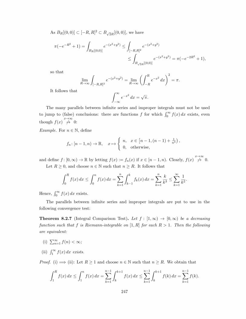
As BR[(0, 0)] ⊂ [−R,R]2 ⊂ B√2R[(0, 0)], we have
π(−e−R2+ 1) =
∫BR[(0,0)]
e−(x2+y2) ≤∫
[−R,R]2e−(x2+y2)
≤∫B√2R[(0,0)]
e−(x2+y2) = π(−e−2R2+ 1),
so that
limR→∞
∫[−R,R]2
e−(x2+y2) = limR→∞
(∫ R
−Re−x
2dx
)2
= π.
It follows that ∫ ∞−∞
e−x2dx =
√π.
The many parallels between infinite series and improper integrals must not be used
to jump to (false) conclusions: there are functions f for which∫∞
0 f(x) dx exists, even
though f(x)x→∞6→ 0:
Example. For n ∈ N, define
fn : [n− 1, n)→ R, x 7→
{n, x ∈
[n− 1, (n− 1) + 1
n3
),
0, otherwise,
and define f : [0,∞)→ R by letting f(x) := fn(x) if x ∈ [n− 1, n). Clearly, f(x)x→∞6→ 0.
Let R ≥ 0, and choose n ∈ N such that n ≥ R. It follows that∫ R
0f(x) dx ≤
∫ n
0f(x) dx =
n∑k=1
∫ k
k−1fk(x) dx =
n∑k=1
k
k3≤∞∑k=1
1
k2.
Hence,∫∞
0 f(x) dx exists.
The parallels between infinite series and improper integrals are put to use in the
following convergence test:
Theorem 8.2.7 (Integral Comparison Test). Let f : [1,∞) → [0,∞) be a decreasing
function such that f is Riemann-integrable on [1, R] for each R > 1. Then the following
are equivalent:
(i)∑∞
n=1 f(n) <∞;
(ii)∫∞
1 f(x) dx exists.
Proof. (i) =⇒ (ii): Let R ≥ 1 and choose n ∈ N such that n ≥ R. We obtain that∫ R
1f(x) dx ≤
∫ n
1f(x) dx =
n−1∑k=1
∫ k+1
kf(x) dx ≤
n−1∑k=1
∫ k+1
kf(k) dx =
n−1∑k=1
f(k).
247

Since∑∞
k=1 f(k) <∞, it follows that∫∞
1 f(x) dx exists.
(ii) =⇒ (i): Let n ∈ N, and note that
n∑k=1
f(k) = f(1) +
n∑k=2
∫ k
k−1f(k) dx
≤ f(1) +
n∑k=2
∫ k
k−1f(x) dx
= f(1) +
∫ n
1f(x) dx
≤ f(1) +
∫ ∞1
f(x) dx.
Hence,∑∞
k=1 f(k) converges.
Examples. 1. Let p > 0 and R > 1, so that∫ R
1
1
xpdx =
{logR, p = 1
11−p
(1
Rp−1 − 1), p 6= 1.
It follows that∫∞
11xp dx exists if and only if p > 1. Consequently,
∑∞n=1
1np converges
if and only if p > 1.
2. Let R > 2. Then change of variables yields that∫ R
2
1
x log xdx =
∫ logR
log 2
1
udu = log u|logR
log 2 = log(logR)− log(log 2).
Consequently,∫∞
21
x log x dx does not exist, and∑∞
n=21
n logn diverges.
3. Does the series∑∞
n=1lognn2 converge?
Let
f : [1,∞)→ R, x 7→ log x
x2.
It follows that
f ′(x) =x− 2x log x
x4≤ 0
for x ≥ 3. Hence, f is decreasing on [3,∞): this is sufficient for the integral
comparison test to be applicable. Let R > 1, and note that∫ R
1
log x
x2dx = − log x
x
∣∣∣∣R1︸ ︷︷ ︸
R→∞→ 0
+
∫ R
1
1
x2dx︸ ︷︷ ︸
=− 1x |R
1
R→∞→ 1
→ 1.
Hence,∫∞
1log xx2
dx exists, and∑∞
n=1lognn2 converges.
248
4. For which θ > 0 does∑∞
n=1( n√θ − 1) converge?
Let
f : [1,∞)→ R, x 7→ θ1x − 1.
First consider the case where θ ≥ 1. Since
f ′(x) = − log θ
x2θ
1x ≤ 0,
and f(x) ≥ 0 for x ≥ 1, the integral comparison test is applicable. For any x ≥ 1,
there is ξ ∈(0, 1
x
)such that
θ1x − 1
1x
= θξ log θ ≥ log θ,
so that
θ1x − 1 ≥ log θ
x
for x ≥ 1. Since∫∞
11x dx does not exist, the comparison test yields that
∫∞1 f(x) dx
does not exist either unless θ = 1. Consequently, if θ ≥ 1, the series∑∞
n=1( n√θ − 1)
converges only if θ = 1.
Consider now the case where θ ≤ 1, the same argument with −f instead of f shows
that∑∞
n=1( n√θ − 1) converges only if θ = 1.
All in all, for θ > 0, the infinite series∑∞
n=1( n√θ− 1) converges if and only if θ = 1.
Exercises
1. Let f : [a, b]→ R be Riemann-integrable. Show that∫ b
af(x) dx = lim
c↑b
∫ c
af(x) dx.
2. Determine whether or not the improper integral∫ ∞0
e−αx cos(βx) dx
exists for α > 0, and evaluate it if possible.
3. Determine whether or not the following improper integrals exist:
(a)∫∞
0x√
1+x3dx;
(b)∫ 1
0dx√sinx
;
(c)∫∞
0 sin(x2) dx.
249

(Hint for (c): Substitute x =√u.)
4. Determine whether or not the improper integral∫ 1
−1
1√1− x2
dx
exists, and evaluate it if possible.
5. For a ∈ R and b ∈ R ∪ {∞} with a < b, let f, g : [a, b)→ R be such that such that:
(a) f and g are both Riemann integrable on [a, c] for each c ∈ [a, b);
(b)∫ ba f(x) dx converges absolutely;
(c) g is bounded.
Show that∫ ba f(x)g(x) dx converges absolutely.
If∫ ba f(x) dx is only required to converge, does then
∫ ba f(x)g(x) dx necessarily con-
verge?
6. Determine those p > 0 for which the series∑∞
n=101
n(logn)(log(logn))p converges.
7. The Gamma Function.
(a) Show that, for all x > 0, the improper integral
Γ(x) :=
∫ ∞0
tx−1e−t dt
exists. (Hint : Show that tx−1e−t ≤ 1t2
for sufficiently large t.)
(b) Show that
xΓ(x) = Γ(x+ 1) (x > 0).
(Hint : Integration by parts.)
(c) Conclude that Γ(n+ 1) = n! for n ∈ N0.
250

Chapter 9
Sequences and Series of Functions
9.1 Uniform Convergence
Definition 9.1.1. Let ∅ 6= D ⊂ RN , and let f, f1, f2, . . . be R-valued functions on D.
Then the sequence (fn)∞n=1 is said to converge pointwise to f on D if
limn→∞
fn(x) = f(x)
holds for each x ∈ D.
Example. For n ∈ N, let
fn : [0, 1]→ R, x 7→ xn,
so that
limn→∞
fn(x) =
{0, x ∈ [0, 1),
1, x = 1.
Let
f : [0, 1]→ R, x 7→
{0, x ∈ [0, 1),
1, x = 1.
It follows that fn → f pointwise on [0, 1].
The example shows one problem with the notion of pointwise convergence: All the
fn’s are continuous whereas f clearly isn’t. To find a better notion of convergence, let us
first rephrase the definition of pointwise convergence:
(fn)∞n=1 converges pointwise to f if, for each x ∈ D and each ε > 0, there is
nx,ε ∈ N such that |fn(x)− f(x)| < ε for all n ≥ nx,ε.
The index nx,ε depends both on x ∈ D and on ε > 0.
The key to a better notion of convergence to functions is to remove the dependence of
the index nx,ε on x:
251

Definition 9.1.2. Let ∅ 6= D ⊂ RN , and let f, f1, f2, . . . be R-valued functions on D.
Then the sequence (fn)∞n=1 is said to converge uniformly to f on D if, for each ε > 0,
there is nε ∈ N such that |fn(x)− f(x)| < ε for all n ≥ nε and for all x ∈ D.
Example. For n ∈ N, let
fn : R→ R, x 7→ sin(nπx)
n.
Since ∣∣∣∣sin(nπx)
n
∣∣∣∣ ≤ 1
n
for all x ∈ R and n ∈ N, it follows that fn → 0 uniformly on R.
Theorem 9.1.3. Let ∅ 6= D ⊂ RN , and let f, f1, f2, . . . be functions on D such that
fn → f uniformly on D and such that f1, f2, . . . are continuous. Then f is continuous.
Proof. Let ε > 0, and let x0 ∈ D. Choose nε ∈ N such that
|fn(x)− f(x)| < ε
3
for all n ≥ nε and for all x ∈ D. Since fnε is continuous, there is δ > 0 such that
|fnε(x)− fnε(x0)| < ε3 for all x ∈ D with ‖x− x0‖ < δ. Fox any such x we obtain:
|f(x)− f(x0)| ≤ |f(x)− fnε(x)|︸ ︷︷ ︸< ε
3
+ |fnε(x)− fnε(x0)|︸ ︷︷ ︸< ε
3
+ |fnε(x0)− f(x0)|︸ ︷︷ ︸< ε
3
< ε.
Hence, f is continuous at x0. Since x0 ∈ D was arbitrary, f is continuos on all of D.
Corollary 9.1.4. Let ∅ 6= D ⊂ RN have content, and let (fn)∞n=1 be a sequence of
continuous functions on D that converges uniformly on D to f : D → R. Then f is
continuous, and we have ∫Df = lim
n→∞
∫Dfn.
Proof. Let ε > 0. Choose nε ∈ N such that
|fn(x)− f(x)| < ε
µ(D) + 1
for all x ∈ D and n ≥ nε. For any n ≥ nε, we thus obtain:∣∣∣∣∫Dfn −
∫Df
∣∣∣∣ ≤ ∫D|fn − f | ≤
∫D
ε
µ(D) + 1=
εµ(D)
µ(D) + 1< ε.
This proves the claim.
Unlike integration, differentiation does not switch with uniform limits:
252

Example. For n ∈ N, let
fn : [0, 1]→ R, x 7→ xn
n,
so that fn → 0 uniformly on [0, 1]. Nevertheless, since
f ′n(x) = xn−1
for x ∈ [0, 1] and n ∈ N, it follows that f ′n 6→ 0 (not even pointwise).
Theorem 9.1.5. Let (fn)∞n=1 be a sequence in C1([a, b]) such that
(a) (fn(x0))∞n=1 converges for some x0 ∈ [a, b];
(b) (f ′n)∞n=1 is uniformly convergent.
Then there is f ∈ C1([a, b]) such that fn → f and f ′n → f ′ uniformly on [a, b].
Proof. Let g : [a, b] → R be such that limn→∞ f′n = g uniformly on [a, b], and let y0 :=
limn→∞ fn(x0). Define
f : [a, b]→ R, x 7→ y0 +
∫ x
x0
g(t) dt.
It follows that f ′ = g, so that f ′n → f ′ uniformly on [a, b].
Let ε > 0, and choose nε ∈ N such that |f ′n(x) − g(x)| < ε2(b−a) for all x ∈ [a, b] and
n ≥ nε and |fn(x0)− y0| < ε2 . For any n ≥ nε and x ∈ [a, b], we then obtain
|fn(x)− f(x)| =∣∣∣∣fn(x0) +
∫ x
x0
f ′n(t) dt− y0 −∫ x
x0
g(t) dt
∣∣∣∣≤ |fn(x0)− y0|+
∣∣∣∣∫ x
x0
f ′n(t) dt−∫ x
x0
g(t) dt
∣∣∣∣<ε
2+
∣∣∣∣∫ x
x0
|f ′n(t)− g(t)| dx∣∣∣∣
≤ ε
2+ε|x− x0|2(b− a)
≤ ε
2+ε
2
= ε.
This proves that fn → f uniformly on [a, b].
Definition 9.1.6. Let ∅ 6= D ⊂ RN . A sequence (fn)∞n=1 of R-valued functions on D
is called a uniform Cauchy sequence on D if, for each ε > 0, there is nε ∈ N such that
|fn(x)− fm(x)| < ε for all x ∈ D and all n,m ≥ nε.
Theorem 9.1.7. Let ∅ 6= D ⊂ RN , and let (fn)∞n=1 be a sequence of R-valued functions
on D. Then the following are equivalent:
253

(i) there is a function f : D → R such that fn → f uniformly on D;
(ii) (fn)∞n=1 is a uniform Cauchy sequence on D.
Proof. (i) =⇒ (ii): Let ε > 0 and choose nε ∈ N such that
|fn(x)− f(x)| < ε
2
for all x ∈ D and n ≥ nε. For x ∈ D and n,m ≥ nε, we thus obtain:
|fn(x)− fm(x)| ≤ |fn(x)− f(x)|+ |f(x)− fm(x)| < ε
2+ε
2= ε.
This proves (ii).
(ii) =⇒ (i): For each x ∈ D, the sequence (fn(x))∞n=1 in R is a Cauchy sequence and
therefore convergent. Define
f : D → R, x 7→ limn→∞
fn(x).
Let ε > 0 and choose nε ∈ N such that
|fn(x)− fm(x)| < ε
2
for all x ∈ D and all n,m ≥ nε. Fix x ∈ D and n ≥ nε. We obtain that
|fn(x)− f(x)| = limm→∞
|fn(x)− fm(x)| ≤ ε
2< ε.
Hence, (fn)∞n=1 converges to f not only pointwise, but uniformly.
Theorem 9.1.8 (Weierstraß M -Test). Let ∅ 6= D ⊂ RN , let (fn)∞n=1 be a sequence of
R-valued functions on D, and suppose that, for each n ∈ N, there is Mn ≥ 0 such that
|fn(x)| ≤Mn for x ∈ D and such that∑∞
n=1Mn <∞. Then∑∞
n=1 fn converges uniformly
and absolutely on D.
Proof. Let ε > 0 and choose nε ∈ N such that
n∑k=m+1
Mk < ε
for all n ≥ m ≥ nε. For all such n and m and for all x ∈ D, we obtain that∣∣∣∣∣n∑k=1
fk(x)−m∑k=1
fk(x)
∣∣∣∣∣ ≤n∑
k=m+1
|fk(x)| ≤n∑
k=m+1
Mk < ε.
Hence, the sequence (∑n
k=1 fk)∞n=1 is uniformly Cauchy on D and thus uniformly conver-
gent. It is easy to see that the convergence is even absolute.
254

Example. Let R > 0, and note that ∣∣∣∣xnn!
∣∣∣∣ ≤ Rn
n!
for all n ∈ N0 and x ∈ [−R,R]. Since∑∞
n=0Rn
n! < ∞, it follows from the M -test that∑∞n=0
xn
n! converges uniformly on [−R,R]. From Theorem 9.1.3, we conclude that exp
is continuous on [−R,R]. Since R > 0 was arbitrary, we obtain the continuity of exp
on all of R. Let x ∈ R be arbitrary. Then there is a sequence (qn)∞n=1 in Q such that
x = limn→∞ qn. Since exp(q) = eq for all q ∈ Q, and since both exp and the exponential
function are continuous, we obtain
exp(x) = limn→∞
exp(qn) = limn→∞
eqn = ex.
Theorem 9.1.9 (Dini’s Lemma). Let ∅ 6= K ⊂ RN be compact and let (fn)∞n=1 a sequence
of continuous functions on K that decreases pointwise to a continuous function f : K → R.
Then (fn)∞n=1 converges to f uniformly on K.
Proof. Let ε > 0. For each n ∈ N, let
Vn := {x ∈ K : fn(x)− f(x) < ε}.
Since each fn − f is continuous, there is an open set Un ⊂ RN such that Un ∩K = Vn.
Let x ∈ K. Since limn→∞ fn(x) = f(x), there is n0 ∈ N such that fn0(x)− f(x) < ε, i.e.
x ∈ Vn0 . It follows that
K =
∞⋃n=1
Vn ⊂∞⋃n=1
Un.
Since K is compact, there are n1, . . . , nk ∈ N such that K ⊂ Un1 ∪ · · · ∪ Unk and hence
K = Vn1 ∪ · · · ∪ Vnk . Let nε := max{n1, . . . , nk}. Since (fn)∞n=1 is a decreasing sequence,
the sequence (Vn)∞n=1 is an increasing sequence of sets. Hence, we have for n ≥ nε that
Vn ⊃ Vnε ⊃ Vnj
for j = 1, . . . , k, and thus Vn = K. For n ≥ nε and x ∈ K, we thus have x ∈ Vn and
therefore
|fn(x)− f(x)| = fn(x)− f(x) < ε.
Hence, we have uniform convergence.
Exercises
1. Let ∅ 6= D ⊂ RN , and let f, f1, f2, . . . : D → R. The sequence (fn)∞n=1 is said to
converge to f locally uniformly on D if, for each x ∈ D, there is a neighborhood U
of x such that (fn)∞n=1 converges to f uniformly on U ∩D.
255

Let ∅ 6= K ⊂ RN be compact, and let f, f1, f2, . . . : K → R be such that (fn)∞n=1
converges to f locally uniformly on K. Show that (fn)∞n=1 converges to f uniformly
on K.
2. For n ∈ N, let
fn : [0,∞)→ R, x 7→ x
n2e−
xn .
Show that fn → 0 uniformly on [0,∞), but that
limn→∞
∫ ∞0
fn(x) dx = 1.
Why doesn’t this contradict Corollary 9.1.4?
3. Show that the series∑∞
n=0xn
n! does not uniformly converge to ex on all of R.
4. Let ∅ 6= D ⊂ RN have content, and let (fn)∞n=1 be a sequence of Riemann-integrable
functions on D that converges uniformly to a function f : D → R. Show that f is
Riemann-integrable as well such that∫Df = lim
n→∞
∫Dfn.
Give an example of a sequence of Riemann-integrable functions on [0, 1] that con-
verges pointwise to a bounded, but not Riemann-integrable function.
9.2 Power Series
Power series can be thought of as “polynomials of infinite degree”:
Definition 9.2.1. Let x0 ∈ R, and let a0, a1, a2, . . . ∈ R. The power series about x0 with
coefficients a0, a1, a2, . . . is the infinite series of functions∑∞
n=0 an(x− x0)n.
This definitions makes no assertion whatsoever about convergence of the series. Whe-
ther or not∑∞
n=0 an(x−x0)n converges depends, of course, on x, and the natural question
that comes up immediately is: Which are the x ∈ R for which∑∞
n=0 an(x−x0)n converges?
Examples. 1. Trivially, each power series∑∞
n=0 an(x− x0)n converges for x = x0.
2. The power series∑∞
n=0xn
n! converges for all x ∈ R.
3. The power series∑∞
n=0 nn(x− π)n converges only for x = π.
4. The power series∑∞
n=0 xn converges if and only if x ∈ (−1, 1).
256

Theorem 9.2.2. Let x0 ∈ R, let a0, a1, a2, . . . ∈ R, and let R > 0 be such that the
sequence (anRn)∞n=0 is bounded. Then the power series
∞∑n=0
an(x− x0)n and
∞∑n=1
nan(x− x0)n−1
converge uniformly and absolutely on [x0 − r, x0 + r] for each r ∈ (0, R).
Proof. Let C ≥ 0 such that |an|Rn ≤ C for all n ∈ N0. Let r ∈ (0, R), and let x ∈[x0 − r, x0 + r]. It follows that
n|an||x− x0|n−1 ≤ n|an|rn−1 = n( rR
)n−1 |an|Rn
R≤ C
Rn( rR
)n−1.
Since rR ∈ (0, 1), the series
∑∞n=1 n
(rR
)n−1converges. By the Weierstraß M -Test, the
power series∑∞
n=1 nan(x− x0)n−1 converges uniformly and absolutely on [x0 − r, x0 + r].
The corresponding claim for∑∞
n=0 an(x− x0)n is proven analogously.
Definition 9.2.3. Let∑∞
n=0 an(x−x0)n be a power series. The radius of convergence of∑∞n=0 an(x− x0)n is defined as
R := sup {r ≥ 0 : (anrn)∞n=0 is bounded} ,
where possibly R =∞ (in case (anrn)∞n=0 is bounded for all r ≥ 0).
If∑∞
n=0 an(x − x0)n has radius of convergence R, then it converges uniformly on
[x0 − r, x0 + r] for each r ∈ [0, R), but diverges for each x ∈ R with |x − x0| > R: this
is an immediate consequence of Theorem 9.2.2 and the fact that (anrn)∞n=1 converges to
zero—and thus is bounded—whenever∑∞
n=0 anrn converges.
And more is true:
Corollary 9.2.4. Let∑∞
n=0 an(x − x0)n be a power series with radius of convergence
R > 0. Then∑∞
n=0 an(x − x0)n converges, for each r ∈ (0, R), uniformly and absolutely
on [x0 − r, x0 + r] to a C1-function f : (x0 − R, x0 + R)→ R of which the first derivative
is given by
f ′(x) =∞∑n=1
nan(x− x0)n−1
for x ∈ (x0 −R, x0 +R). Moreover, F : (x0 −R, x0 +R)→ R given by
F (x) :=
∞∑n=0
ann+ 1
(x− x0)n+1
for x ∈ (x0 −R, x0 +R) is an antiderivative of f .
Proof. Just combine Theorems 9.2.2 and 9.1.5.
257

In short, Corollary 9.2.4 asserts that power series can be differentiated and integrated
term by term.
Examples. 1. For x ∈ (−1, 1), we have
∞∑n=1
nxn = x∞∑n=1
nxn−1
= x
∞∑n=0
d
dxxn
= xd
dx
∞∑n=0
xn, by Corollary 9.2.4,
= xd
dx
1
1− x=
x
(1− x)2.
2. For x ∈ (−1, 1), we have
1
x2 + 1=
1
1− (−x2)=∞∑n=0
(−1)nx2n.
Corollary 9.2.4 yields C ∈ R such that
arctanx+ C =∞∑n=0
(−1)nx2n+1
2n+ 1
for all x ∈ (−1, 1). Letting x = 0, we see that C = 0, so that
arctanx =∞∑n=0
(−1)nx2n+1
2n+ 1
for x ∈ (−1, 1).
3. For x ∈ (0, 2), we have
1
x=
1
1− (1− x)=∞∑n=0
(1− x)n =∞∑n=0
(−1)n(x− 1)n.
By Corollary 9.2.4, there is C ∈ R such that
log x+ C =
∞∑n=0
(−1)n
n+ 1(x− 1)n+1 =
∞∑n=1
(−1)n−1
n(x− 1)n
for x ∈ (0, 2). Letting x = 1, we obtain that C = 0, so that
log x =∞∑n=1
(−1)n−1
n(x− 1)n
for x ∈ (0, 2).
258

Proposition 9.2.5 (Cauchy–Hadamard Formula). The radius of convergence R of the
power series∑∞
n=0 an(x− x0)n is given by
R =1
lim supn→∞n√|an|
,
where the convention applies that 10 =∞ and 1
∞ = 0.
Proof. Let
R′ :=1
lim supn→∞n√|an|
.
Let x ∈ R \ {x0} be such that |x− x0| < R′, so that
lim supn→∞
n√|an| <
1
|x− x0|.
Let θ ∈(
lim supn→∞n√|an|, 1
|x−x0|
). From the definition of lim sup, we obtain n0 ∈ N
such thatn√|an| < θ
for n ≥ n0 and therefore
n√|an||x− x0|n < θ|x− x0| < 1
for n ≥ n0. Hence, by the root test,∑∞
n=0 an(x− x0)n converges, so that R′ ≤ R.
Let x ∈ R such that |x− x0| > R′, i.e.,
lim supn→∞
n√|an| >
1
|x− x0|.
By Proposition B.1.5, there is a subsequence (ank)∞k=1 of (an)∞n=0 such that we have
lim supn→∞n√|an| = limk→∞
nk√|ank |. Without loss of generality, we may suppose that
nk
√|ank | >
1
|x− x0|
for all k ∈ N and thusnk
√|ank ||x− x0|nk > 1
for k ∈ N. Consequently, (an(x−x0)n)∞n=0 does not converge to zero, so that∑∞
n=0 an(x−x0)n has to diverge. It follows that R ≤ R′.
Examples. 1. Consider the power series,
∞∑n=1
(1 +
1
n
)n2
xn,
259

so thatn√an =
(1 +
1
n
)nfor n ∈ N. It follows from the Cauchy–Hadamard Formula that
limn→∞
n√an = lim
n→∞
(1 +
1
n
)n= e,
so that 1e is the radius of convergence of the power series.
2. We will now use the Cauchy–Hadamard formula to prove that limn→∞ n√n = 1.
Since∑∞
n=1 nxn converges for |x| < 1 and diverges for |x| > 1, the radius of conver-
gence R of that series must equal 1. By the Cauchy–Hadamard formula, this means
that lim supn→∞n√n = 1. Hence, 1 is the largest accumulation point of ( n
√n)∞n=1.
Since, trivially, n√n ≥ 1 for all n ∈ N, all accumulation points of the sequence must
be greater or equal to 1. Hence, ( n√n)∞n=1 has only one accumulation point, namely
1, and therefore converges to 1.
Definition 9.2.6. We say that a function f has a series expansion about x0 ∈ R if
f(x) =∑∞
n=0 an(x− x0)n for some power series∑∞
n=0 an(x− x0)n and all x in some open
interval centered at x0.
From Corollary 9.2.4, we obtain immediately:
Corollary 9.2.7. Let f be a function with a power series expansion∑∞
n=0 an(x − x0)n
about x0 ∈ R. Then f is infinitely often differentiable on an open interval about x0, i.e.,
a C∞-function, such that
an =f (n)(x0)
n!
holds for all n ∈ N0. In particular, the power series expansion of f about x0 is unique.
Let f be a function that is infinitely often differentiable on some neighborhood of
x0 ∈ R. Then the Taylor series of f at x0 is the power series∑∞
n=0f (n)(x0)
n! (x − x0)n.
Corollary 9.2.7 asserts that, whenever f has a power series expansion about x0, then the
corresponding power series must be the function’s Taylor series. We thus may also speak
of the Taylor expansion of f about x0.
Does every C∞-function have a Taylor expansion?
Example. Let F be the collection of all functions f : R→ R of the following form: There
is a polynomial p such that
f(x) =
{p(
1x
)e−
1x2 , x 6= 0,
0, x = 0,(9.1)
260

for all x ∈ R. It is clear that each f ∈ F is continuous on R\{0}, and from de l’Hospital’s
Rule, it follows that each f ∈ F is also continuous at x = 0.
We claim that each f ∈ F is differentiable such that f ′ ∈ F .
Let f ∈ F be as in (9.1). It is easy to see that f is differentiable at each x 6= 0 with
f ′(x) = − 1
x2p′(
1
x
)e−
1x2 + p
(1
x
)(− 2
x3
)e−
1x2
=
(− 1
x2p′(
1
x
)− 2
x3p
(1
x
))e−
1x2 ,
so that
f ′(x) = q
(1
x
)e−
1x2
for such x, where
q(y) := −y2p′(y)− 2y3p(y)
for all y ∈ R. Let r(y) := y p(y) for y ∈ R, so that r is a polynomial. Since functions in
F are continuous at x = 0, we see that
limh→0h6=0
f(h)− f(0)
h= lim
h→0h6=0
1
hp
(1
h
)e−
1h2 = lim
h→0h6=0
r
(1
h
)e−
1h2 = 0.
This proves the claim.
Consider
f : R→ R, x 7→
{e−
1x2 , x 6= 0,
0, x = 0,
so that f ∈ F . By the claim just proven, it follows that f is a C∞-function with f (n) ∈ Ffor all n ∈ N. In particular, f (n)(0) = 0 holds for all n ∈ N. The Taylor series of f thus
converges (to 0) on all of R, but f does not have a Taylor expansion about 0.
Theorem 9.2.8. Let x0 ∈ R, let R > 0, and let f ∈ C∞([x0 − R, x0 + R]) such that the
set
{|f (n)(x)| : x ∈ [x0 −R, x0 +R], n ∈ N0} (9.2)
is bounded. Then
f(x) =
∞∑n=0
f (n)(x0)
n!(x− x0)n
holds for all x ∈ [x0 −R, x0 +R] with uniform convergence on [x0 −R, x0 +R]
Proof. Let C ≥ 0 be an upper bound for (9.2), and let x ∈ [x0 − R, x0 + R]. For each
n ∈ N, Taylor’s theorem yields ξ ∈ [x0 −R, x0 +R] such that
f(x) =
n∑k=0
f (k)(x0)
k!(x− x0)k +
f (n+1)(ξ)
(n+ 1)!(x− x0)n+1,
261

so that ∣∣∣∣∣f(x)−n∑k=0
f (k)(x0)
k!(x− x0)k
∣∣∣∣∣ =
∣∣∣∣∣f (n+1)(ξ)
(n+ 1)!
∣∣∣∣∣ |x− x0|n+1 ≤ C Rn+1
(n+ 1)!.
Since limn→∞Rn+1
(n+1)! = 0, this completes the proof.
Example. For all x ∈ R,
sinx =∞∑n=0
(−1)nx2n+1
(2n+ 1)!and cosx =
∞∑n=0
(−1)nx2n
(2n)!
holds.
Let∑∞
n=0 an(x− x0)n be a power series with radius of convergence R. What happens
if x = x0 ±R?
In general, nothing can be said.
Theorem 9.2.9 (Abel’s Theorem). Suppose that the series∑∞
n=0 an converges. Then the
power series∑∞
n=0 anxn converges pointwise on (−1, 1] to a continuous function.
Proof. For x ∈ (−1, 1], define
f(x) :=∞∑n=0
anxn.
Since∑∞
n=1 anxn converges uniformly on all compact subsets of (−1, 1), it is clear that
f is continuous on (−1, 1). What remains to be shown is that f is continuous at 1, i.e.,
limx↑1 f(x) = f(1).
For n ∈ Z with n ≥ −1, define rn :=∑∞
k=n+1 ak. It follows that r−1 = f(1), rn−rn−1 =
−an for all n ∈ N0, and limn→∞ rn = 0. Since (rn)∞n=−1 is bounded, the series∑∞
n=0 rnxn
and∑∞
n=0 rn−1xn converge for x ∈ (−1, 1). We obtain for x ∈ (−1, 1) that
(1− x)
∞∑n=0
rnxn =
∞∑n=0
rnxn −
∞∑n=0
rnxn+1
=∞∑n=0
rnxn −
∞∑n=0
rn−1xn + r−1
=
∞∑n=0
(rn − rn−1)xn + r−1
= −∞∑n=1
anxn
︸ ︷︷ ︸=f(x)
+f(1),
i.e.,
f(1)− f(x) = (1− x)∞∑n=0
rnxn.
262

Let ε > 0 and let C ≥ 0 be such that |rn| ≤ C for n ≥ −1. Choose nε ∈ N such that
|rn| ≤ ε2 for n ≥ nε, and set δ := ε
2Cnε+1 . Let x ∈ (0, 1) such that 1 − x < δ. It follows
that
|f(1)− f(x)| ≤ (1− x)∞∑n=0
|rn|xn
= (1− x)
nε−1∑n=0
|rn|xn + (1− x)∞∑
n=nε
|rn|xn
≤ (1− x)Cnε + (1− x)ε
2
∞∑n=nε
xn
<ε
2+ (1− x)
ε
2
∞∑n=0
xn︸ ︷︷ ︸= 1
1−x
=ε
2+ε
2
= ε,
so that f is indeed continuous at 1.
Examples. 1. For x ∈ (−1, 1), the identity
log(x+ 1) =
∞∑n=1
(−1)n−1
nxn (9.3)
holds. By Abel’s Theorem, the right hand side of (9.3) defines a continuous function
on all of (−1, 1]. Since the left hand side of (9.3) is also continuous on (−1, 1], it
follows that (9.3) holds for all x ∈ (−1, 1]. Letting x = 1, we obtain that
∞∑n=1
(−1)n−1
n= log 2.
2. Since
arctanx =∞∑n=0
(−1)nx2n+1
2n+ 1
holds for all x ∈ (−1, 1), a similar argument as in the previous example yields that
this identity holds for all x ∈ (−1, 1]. In particular, letting x = 1 yields
π
4= arctan 1 =
∞∑n=0
(−1)n
2n+ 1.
263

Exercises
1. Determine the radii of convergence for the following power series:
(a)∑∞
n=0
(2nn
)xn;
(b)∑∞
n=2(−1)n(
5n+33n−4
)n(x− 2018)n;
(c)∑∞
n=01nn (x− e)n;
(d)∑∞
n=0nn
n! (x− 6)n.
2. Let (an)∞n=0 be a sequence in R such that R := limn→∞|an||an+1| exists. Show that R,
for any x0 ∈ R, is the radius of convergence of the power series∑∞
n=0 an(x− x0)n.
3. Show that the power series∑∞
n=1 n2xn has radius of convergence 1 and that
∞∑n=1
n2xn =x(x+ 1)
(1− x)3
for x ∈ (−1, 1).
4. For any α ∈ R and n ∈ N0, let(α
n
):=
n∏j=1
α− j + 1
j.
You may use without proving it that(α− 1
n
)+
(α− 1
n− 1
)=
(α
n
)(9.4)
for n ∈ N.
(a) Show that the binomial series∑∞
n=0
(αn
)xn converges on (−1, 1) to a differen-
tiable function f .
(b) Show that (1 + x)f ′(x) = αf(x) for x ∈ (−1, 1) .
Hint : Use (9.4).
(c) Conclude that∞∑n=0
(α
n
)xn = (1 + x)α
for x ∈ (−1, 1).
Hint : Let g(x) := (1 + x)α, consider f(x)/g(x), and differentiate.
264

5. Although the theory of power series was developed in class only for real variables,
it all works perfectly well over C as well. We can thus extend exp, sin, and cos to Cby defining
ez :=
∞∑n=0
zn
n!, sin z :=
∞∑n=0
(−1)nz2n+1
(2n+ 1)!, and cos z :=
∞∑n=0
(−1)nz2n
(2n)!
for z ∈ C.
Show that
eiz = cos z + i sin z
holds for all z ∈ C, and derive Euler’s Identity : eiπ + 1 = 0.
9.3 Fourier Series
The theory of Fourier series is about approximating periodic functions through terms
involving sine and cosine.
Definition 9.3.1. Let ω > 0, and let PCω(R) denote the collection of all functions
f : R→ R with the following properties:
(a) f(x+ ω) = f(x) for x ∈ R.
(b) there is a partition −ω2 = t0 < t1 < · · · < tn = ω
2 of[−ω
2 ,ω2
]such that f is continuous
on (tj−1, tj) for j = 1, . . . , n and such that limt↑tj f(t) exists for j = 1, . . . , n and
limt↓tj f(t) exists for j = 0, . . . , n− 1.
We will focus on the case where ω = 2π.
Example. The functions sin and cos belong to PC2π(R).
ω
2
t1t
2ω
2−
x
y
Figure 9.1: A function in PCω(R)
265

How can we approximate arbitrary f ∈ PC2π(R) by linear combinations of sin and
cos?
Definition 9.3.2. For f ∈ PC2π(R), the Fourier coefficients a0, a1, a2, . . . , b1, b2, . . . of f
are defined as
an :=1
π
∫ π
−πf(t) cos(nt) dt
for n ∈ N0 and
bn :=1
π
∫ π
−πf(t) sin(nt) dt
for n ∈ N. The infinite series a02 +
∑∞n=1(an cos(nx) + bn sin(nx)) is called the Fourier
series of f . We write
f(x) ∼ a0
2+∞∑n=1
(an cos(nx) + bn sin(nx)).
The fact that
f(x) ∼ a0
2+
∞∑n=1
(an cos(nx) + bn sin(nx))
does not mean that we have convergence—not even pointwise.
Example. Let
f : (−π, π]→ R, x 7→
{−1, x ∈ (−π, 0),
1, x ∈ [0, π].
Extend f to a function in PC2π(x) (using Definition 9.3.2(a)). For n ∈ N0, we obtain
an =1
π
∫ π
−πf(t) cos(nt) dt
=1
π
(−∫ 0
−πcos(nt) dt+
∫ π
0cos(nt) dt
)=
1
π
(−∫ π
0cos(nt) dt+
∫ π
0cos(nt) dt
)= 0.
266
For n ∈ N, we have
bn =1
π
∫ π
−πf(t) sin(nt) dt
=1
π
(−∫ 0
−πsin(nt) dt+
∫ π
0sin(nt) dt
)=
1
π
(− 1
n
∫ 0
−πnsin(t) dt+
1
n
∫ πn
0sin(t) dt
)=
1
πn
(cos t|0−πn − cos t|πn0
)=
1
πn(1− cos(πn)− cos(nπ) + 1)
=2− 2 cos(πn)
πn
=
{0, n even,4πn , n odd.
It follows that
f(x) ∼ 4
π
∞∑n=0
1
2n+ 1sin((2n+ 1)x).
The Fourier series converges to zero whenever x is an integer multiple of π, i.e., it does
not converge to f for such x.
In general, it is too much to expect pointwise convergence. Suppose that f ∈ PC2π(R)
has a Fourier series that converges pointwise to f . Let g : R → R be another function in
PC2π(R) obtained from f by altering f at finitely many points in (−π, π]. Then f and g
have the same Fourier series, but at those points where f differs from g, the series cannot
converge pointwise to g.
We need a different type of convergence.
Definition 9.3.3. For f ∈ PC2π(R), define
‖f‖2 :=
(∫ π
−π|f(t)|2 dt
) 12
.
Proposition 9.3.4. Let f, g ∈ PC2π(R), and let λ ∈ R. Then we have:
(i) ‖f‖2 ≥ 0;
(ii) ‖λf‖2 = |λ|‖f‖2;
(iii) ‖f + g‖2 ≤ ‖f‖2 + ‖g‖2.
Proof. (i) and (ii) are obvious.
267

For (iii), we first claim that∫ π
−π|f(t)g(t)| dt ≤ ‖f‖2‖g‖2 (9.5)
Let ε > 0, and choose a partition −π = t0 < · · · < tn = π and support points ξj ∈ (tj−1, tj)
for j = 1, . . . , n such that∣∣∣∣∣∣∫ π
−π|f(t)g(t)| dt−
n∑j=1
|f(ξj)g(ξj)|(tj − tj−1)
∣∣∣∣∣∣ < ε,
∣∣∣∣∣∣∣(∫ π
−π|f(t)|2 dt
) 12
−
n∑j=1
|f(ξj)|2(tj − tj−1)
12
∣∣∣∣∣∣∣ < ε,
and ∣∣∣∣∣∣∣(∫ π
−π|g(t)|2 dt
) 12
−
n∑j=1
|g(ξj)|2(tj − tj−1)
12
∣∣∣∣∣∣∣ < ε.
We therefore obtain∫ π
−π|f(t)g(t)| dt <
n∑j=1
|f(ξj)g(ξj)|(tj − tj−1) + ε
=n∑j=1
|f(ξj)|(tj − tj−1)12 |g(ξj)|(tj − tj−1)
12 + ε
≤
n∑j=1
|f(ξj)|2(tj − tj−1)
12 n∑j=1
|g(ξj)|2(tj − tj−1)
12
+ ε,
by the Cauchy–Schwarz Inequality,
<
((∫ π
−π|f(t)|2 dt
) 12
+ ε
)((∫ π
−π|g(t)|2 dt
) 12
+ ε
)+ ε.
Since ε > 0 is arbitrary, this yields (9.5).
Since
‖f + g‖22 =
∫ π
−π(f(t)2 + 2f(t)g(t) + g(t)2) dt
=
∫ π
−π|f(t)|2 dt+ 2
∫ π
−πf(t)g(t) dt+
∫ π
−π|g(t)|2 dt
≤ ‖f‖22 + 2
∫ π
−π|f(t)g(t)| dt+ ‖g‖22
≤ ‖f‖22 + 2‖f‖2‖g‖2 + ‖g‖22, by (9.5),
= (‖f‖2 + ‖g‖2)2,
268
this proves (iii).
One cannot improve Proposition 9.3.4(i) to ‖f‖2 > 0 for non-zero f : Any function f
that is different from zero only in finitely many points provides a counterexample.
Definition 9.3.5. Let α0, α1, . . . , αn, β1, . . . , βn ∈ R. A function of the form
Tn(x) =α0
2+
n∑k=1
(αk cos(kx) + βk sin(kx)) (9.6)
for x ∈ R is called a trigonometric polynomial of degree n.
Is is obvious that trigonometric polynomials belong to PC2π(R).
Lemma 9.3.6. Let f ∈ PC2π(R) have the Fourier coefficients a0, a1, a2 . . . , b1, b2, . . ., and
let Tn be a trigonometric polynomial of degree n ∈ N as in (9.6). Then we have
‖f − Tn‖22
= ‖f‖22 − π
(a2
0
2+
n∑k=1
(a2k + b2k)
)+ π
(1
2(α0 − a0)2 +
n∑k=1
((αk − ak)2 + (βk − bk)2)
).
Proof. First note that
‖f − Tn‖22 =
∫ π
−πf(t)2 dt︸ ︷︷ ︸
=‖f‖22
−2
∫ π
−πf(t)Tn(t) dt+
∫ π
−πTn(t)2 dt.
Then, observe that∫ π
−πf(t)Tn(t) dt
=α0
2
∫ π
−πf(t) dt+
n∑k=1
αk
∫ π
−πf(t) cos(kt) dt+
n∑k=1
βk
∫ π
−πf(t) sin(kt) dt
= π
(α0
2a0 +
n∑k=1
(αkak + βkbk)
),
269

and, moreover, that∫ π
−πTn(t)2 dt
= 2πα2
0
4+α0
2
n∑k=1
(αk
∫ π
−πcos(kt) dt︸ ︷︷ ︸
=0
+βk
∫ π
−πsin(kt) dt︸ ︷︷ ︸
=0
)
+
n∑k,j=1
(αkαj
∫ π
−πcos(kt) cos(jt) dt+ 2αkβj
∫ π
−πcos(kt) sin(jt) dt
+ βkβj
∫ π
−πsin(kt) sin(jt) dt
)= π
α20
2+
n∑k=1
(α2k
∫ π
−πcos(kt)2 dt+ β2
k
∫ π
−πsin(kt)2 dt
)
= π
(α2
0
2+
n∑k=1
(α2k + β2
k)
).
We thus obtain
‖f − Tn‖22
= ‖f‖22 + π
(−α0a0 −
n∑k=1
(2αkak + 2βkbk) +α2
0
2+
n∑k=1
(α2k + β2
k)
)
= ‖f‖22 + π
(1
2(α2
0 − 2α0a0) +
n∑k=1
(α2k − 2αkak + β2
k − 2βkbk)
)
= ‖f‖22 + π
(1
2(α0 − a0)2 +
n∑k=1
((αk − ak)2 + (βk − bk)2)− 1
2a2
0 −n∑k=1
(a2k + b2k)
)This proves the claim.
Proposition 9.3.7. For f ∈ PC2π(R) with the Fourier coefficients a0, a1, a2 . . . , b1, b2, . . .
and n ∈ N, let Sn(f) ∈ PC2π(R) be given by
Sn(f)(x) =a0
2+
n∑k=1
(ak cos(kx) + bk sin(kx))
for x ∈ R. Then Sn(f) is the unique trigonometric polynomial Tn of degree n for which
‖f − Tn‖2 becomes minimal. In fact, we have
‖f − Sn(f)‖22 = ‖f‖22 − π
(a2
0
2+
n∑k=1
(a2k + b2k)
).
Corollary 9.3.8 (Bessel’s Inequality). Let f ∈ PC2π(R) have the Fourier coefficients
a0, a1, a2 . . . , b1, b2, . . .. Then we have the inequality
a20
2+∞∑n=1
(a2n + b2n) ≤ 1
π‖f‖22.
270
In particular, limn→∞ an = limn→∞ bn = 0 holds.
Definition 9.3.9. Let n ∈ N0. The n-th Dirichlet kernel is defined on [−π, π] by letting
Dn(t) :=
sin((n+ 1
2)t)2 sin( 1
2t)
, 0 < |t| ≤ π,
n+ 12 , t = 0.
Lemma 9.3.10. Let f ∈ PC2π(R). Then
Sn(f)(x) =1
π
∫ π
−πf(x+ t)Dn(t) dt
for all n ∈ N0 and x ∈ [−π, π].
Proof. Let n ∈ N0 and let x ∈ [−π, π]. We have
Sn(f)(x) =1
2π
∫ π
−πf(t) dt+
1
π
∫ π
−π
n∑k=1
f(t)(cos(kx) cos(kt) + sin(kx) sin(kt)) dt
=1
π
∫ π
−πf(t)
(1
2+
n∑k=1
(cos(kx) cos(−kt)− sin(kx) sin(−kt))
)dt
=1
π
∫ π
−πf(t)
(1
2+
n∑k=1
cos(k(x− t))
)dt
=1
π
∫ π+x
−π−xf(x+ s)
(1
2+
n∑k=1
cos(ks)
)ds
=1
π
∫ π
−πf(x+ s)
(1
2+
n∑k=1
cos(ks)
)ds.
We now claim that
Dn(s) =1
2+
n∑k=1
cos(ks)
holds for all s ∈ [−π, π]. First note that, for any s ∈ R and k ∈ Z, the identity
2 cos(ks) sin
(1
2s
)= sin
((k +
1
2
)s
)− sin
((k − 1
2
)s
).
Hence, we obtain for s ∈ [−π, π] and n ∈ N0 that
2 sin
(1
2s
) n∑k=1
cos(ks) =n∑k=1
(sin
((k +
1
2
)s
)− sin
((k − 1
2
)s
))= sin
((n+
1
2
)s
)− sin
(1
2s
)and thus, for s 6= 0,
n∑k=1
cos(ks) =sin((n+ 1
2
)s)− sin
(12s)
2 sin(
12s) = Dn(s)− 1
2;
271

for s = 0, the left and the right hand side of the previous equation also coincide as is
checked immediately.
Lemma 9.3.11 (Riemann–Lebesgue Lemma). For f ∈ PC2π(R), we have that
limn→∞
∫ π
−πf(t) sin
((n+
1
2
)t
)dt = 0.
Proof. Note that, for n ∈ N, we have∫ π
−πf(t) sin
((n+
1
2
)t
)dt
=
∫ π
−πf(t)
(cos
(1
2t
)sin(nt) + sin
(1
2t
)cos(nt)
)dt
=1
π
∫ π
−π
(πf(t) cos
(1
2t
))sin(nt) dt
+1
π
∫ π
−π
(πf(t) sin
(1
2t
))cos(nt) dt.
Since 1π
∫ π−π(πf(t) cos
(12 t))
sin(nt) dt and 1π
∫ π−π(πf(t) sin
(12 t))
cos(nt) dt are Fourier co-
efficients, it follows from Bessel’s Inequality that
limn→∞
1
π
∫ π
−π
(πf(t) cos
(1
2t
))sin(nt) dt = lim
n→∞
1
π
∫ π
−π
(πf(t) sin
(1
2t
))cos(nt) dt = 0.
This proves the claim.
Definition 9.3.12. Let f : R→ R, and let x ∈ R. We say that:
(a) f has a right hand derivative at x if
limh↓0
f(x+ h)− f(x+)
h
exists, where f(x+) := limh↓0 f(x+ h) is supposed to exist.
(b) f has a left hand derivative at x if
limh↑0
f(x+ h)− f(x−)
h
exists, where f(x−) := limh↑0 f(x+ h) is supposed to exist.
Theorem 9.3.13. Let f ∈ PC2π(R) and suppose that f has left and right hand derivatives
at x ∈ R. Then
a0
2+∞∑n=1
(an cos(nx) + bn sin(nx)) =1
2(f(x+) + f(x−))
holds.
272

Proof. In the proof of Lemma 9.3.10, we saw that
1
2+
n∑k=1
cos(kt) = Dn(t)
holds for all t ∈ [−π, π] and n ∈ N0, so that
1
π
∫ π
0f(x+)Dn(t) dt =
1
2f(x+) +
n∑k=1
1
π
∫ π
0f(x+) cos(kt) dt︸ ︷︷ ︸
=0
=1
2f(x+)
and similarly1
π
∫ 0
−πf(x−)Dn(t) dt =
1
2f(x−).
for n ∈ N. It follows that
Sn(f)(x)− 1
2(f(x+) + f(x−))
=1
π
∫ π
−πf(x+ t)Dn(t) dt− 1
π
∫ π
0f(x+)Dn(t) dt− 1
π
∫ 0
−πf(x−)Dn(t) dt
=1
π
∫ 0
−π
f(x+ t)− f(x−)
2 sin(
12 t) sin
((n+
1
2
)t
)dt
+1
π
∫ π
0
f(x+ t)− f(x+)
2 sin(
12 t) sin
((n+
1
2
)t
)dt
holds for n ∈ N. Define g : (−π, π]→ R by letting
g(t) :=
0, t ∈ (−π, 0),f(x+t)−f(x+)
2 sin( 12t)
, t ∈ (0, π].
Since
limt↓0
f(x+ t)− f(x+)
2 sin(
12 t) = lim
t↓0
f(x+ t)− f(x+)
t
t
2 sin(
12 t) = lim
t↓0
f(x+ t)− f(x+)
t
exists, it follows that g ∈ PC2π(R). From the Riemann–Lebesgue Lemma, it follows that
limn→∞
∫ π
0
f(x+ t)− f(x+)
2 sin(
12 t) sin
((n+
1
2
)t
)dt = lim
n→∞
∫ π
−πg(t) sin
((n+
1
2
)t
)dt = 0
and, analogously,
limn→∞
∫ 0
−π
f(x+ t)− f(x−)
2 sin(
12 t) sin
((n+
1
2
)t
)dt = 0.
This completes the proof.
273

Example. Let
f : (−π, π]→ R, x 7→
{−1, x ∈ (−π, 0),
1, x ∈ [0, π].
It follows that
f(x) =4
π
∞∑n=0
1
2n+ 1sin((2n+ 1)x)
for all x that are not integer multiples of π.
Corollary 9.3.14. Let f ∈ PC2π(R) be continuous and piecewise differentiable. Then
a0
2+∞∑n=1
(an cos(nx) + bn sin(nx)) = f(x)
holds for all x ∈ R.
Theorem 9.3.15. Let f ∈ PC2π(R) be continuous and piecewise continuously differen-
tiable. Thena0
2+∞∑n=1
(an cos(nx) + bn sin(nx)) = f(x) (9.7)
holds for all x ∈ R with uniform convergence on R.
Proof. Let −π = t0 < · · · < tm = π be such that f is continuously differentiable on
[tj−1, tj ] for j = 1, . . . ,m. Then f ′(t) exists for t ∈ [−π, π]—except possibly for t ∈{t0, . . . , tn}—and thus gives rise to a function in PC2π(R), which we shall denote by f ′
for the sake of simplicity.
Let a′0, a′1, a′2, . . . , b
′1, b′2, . . . be the Fourier coefficients of f ′. For n ∈ N, we obtain that
a′n =1
π
∫ π
−πf ′(t) cos(nt) dt
=1
π
m∑j=1
∫ tj
tj−1
f ′(t) cos(nt) dt
=1
π
m∑j=1
(f(t) cos(nt)|tjtj−1
+ n
∫ tj
tj−1
f(t) sin(nt) dt
)
=n
π
∫ π
−πf(t) sin(nt) dt
= nbn
and, in a similar vein,
b′n = −nan.
From Bessel’s Inequality, we know that∑∞
n=1(b′n)2 < ∞, and from the Cauchy–Schwarz
Inequality , we conclude that
∞∑n=1
|an| =∞∑n=1
1
n|b′n| ≤
( ∞∑n=1
1
n2
) 12( ∞∑n=1
(b′n)2
) 12
<∞;
274
analogously, we see that∑∞
n=1 |bn| <∞ as well.
Since
|an cos(nx) + bn sin(nx)| ≤ |an|+ |bn|
for all x ∈ R, the Weierstraß M -Test yields that the Fourier series a02 +
∑∞n=1(an cos(nx)+
bn sin(nx)) converges uniformly on R. Since the identity (9.7) holds pointwise by Corollary
9.3.14, the uniform limit of the Fourier series must be f .
Example. Let f ∈ PC2π(R) be given by f(x) := x2 for x ∈ (−π, π]. It is easy to see that
bn = 0 for all n ∈ N.
We have
a0 =1
π
∫ π
−πt2 dt =
1
π
(t3
3
∣∣∣∣π−π
)=
1
π
(π3
3+π3
3
)=
2π2
3.
For n ∈ N, we compute
an =1
π
∫ π
−πt2 cos(nt) dt
=1
π
(t2
nsin(nt)
∣∣∣∣π−π− 2
n
∫ π
−πt sin(nt) dt
)= − 2
πn
∫ π
−πt sin(nt) dt
= − 2
πn
(− tn
cos(nt)
∣∣∣∣π−π
+1
n
∫ π
−πcos(nt) dt
)=
4
n2cos(πn)
= (−1)n4
n2.
Hence, we have the identity
f(x) =π2
3+
∞∑n=1
(−1)n4
n2cos(nx)
with uniform convergence on all of R.
Letting x = 0, we obtain
0 =π2
3+∞∑n=1
(−1)n4
n2,
so thatπ2
12=
∞∑n=1
(−1)n−1
n2.
Letting x = π yields
π2 =π2
3+∞∑n=1
(−1)n4
n2(−1)n =
π2
3+∞∑n=1
4
n2
275
and thus∞∑n=1
1
n2=π2
6.
For our last two theorems, we require the following lemma:
Lemma 9.3.16. Let a < b, let f : [a, b] → R be continuous, and let ε > 0. Then there is
a continuous, piecewise linear function g : [a, b] → R such that g(a) = f(a), g(b) = f(b),
and |f(t)− g(t)| < ε for all t ∈ [a, b].
Proof. As [a, b] is compact and f is continuous, f is uniformly continuous. Choose δ > 0
such that |f(s) − f(t)| < ε2 for s, t ∈ [a, b] with |s − t| < δ. Let a = t0 < · · · < tn = b
be a partition of [a, b] with maxj=1,...,n |tj − tj−1| < δ. Define g : [a, b] → R as follows: if
t ∈ [tj−1, tj ] with j ∈ {1, . . . , n}, let
g(t) :=1
tj − tj−1((tj − t)f(tj−1)− (tj−1 − t)f(tj)).
Then g is a piecewise linear, continuous functions with g(tj) = f(tj) for j = 1, . . . , n. Let
t ∈ [a, b], and let j ∈ {1, . . . , n} be such that t ∈ [tj−1, tj ]. We obtain
|f(t)− g(t)| =∣∣∣∣f(t)− 1
tj − tj−1((tj − t)f(tj−1)− (tj−1 − t)f(tj))
∣∣∣∣=
∣∣∣∣ 1
tj − tj−1((tj − t)f(t)− (tj−1 − t)f(t))
− 1
tj − tj−1((tj − t)f(tj−1)− (tj−1 − t)f(tj))
∣∣∣∣≤ 1
tj − tj−1(|tj − t||f(t)− f(tj−1)|+ |tj−1 − t||f(t)− f(tj−1)|)
≤ tj − tj−1
tj − tj−1(|f(t)− f(tj−1)|+ |f(t)− f(tj)|)
= |f(t)− f(tj−1)|︸ ︷︷ ︸< ε
2
+ |f(t)− f(tj)|︸ ︷︷ ︸< ε
2
< ε.
276

a b
f
g
x
y
Figure 9.2: The functions f and g
This proves the claim.
Theorem 9.3.17 (Weierstraß’ Approximation Theorem). Let a < b, let f : [a, b]→ R be
continuous, and let ε > 0. Then there is a polynomial p such that |f(t) − p(t)| < ε for
t ∈ [a, b]. In particular, there is a sequence of polynomials that converges to f uniformly
on [a, b].
Proof. Without loss of generality that a = −π and b = π.
Consider first the case where f(−π) = 0 = f(π). We can then extend f to a continuous
function in PC2π(R) (likewise denoted by f). By Lemma 9.3.16, there is a continuous,
piecewiese linear function g : [−π, π]→ R such that g(−π) = g(π) = 0 and |f(t)−g(t)| < ε3
for t ∈ [−π, π]. Extend g to a function in PC2π(R) (also denoted by g). As g is, in
particular, piecewise continuously differentiable, Theorem 9.3.15 yields nε ∈ N such that
|g(t)−Sn(g)(t)| < ε3 for all n ≥ nε and all t ∈ [−π, π]. For k = 1, . . . , n, the Taylor series of
cos(kt) and sin(kt) converge uniformly to those functions on [−π, π]. Cutting these series
off after sufficiently many summands, we obtain a polynomial p with |Snε(g)(t)−p(t)| < ε3
for all t ∈ [−π, π]. Consequently,
|f(t)− p(t)| ≤ |f(t)− g(t)|︸ ︷︷ ︸< ε
3
+ |g(t)− Snε(g)(t)|︸ ︷︷ ︸< ε
3
+ |Snε(g)(t)− p(t)|︸ ︷︷ ︸< ε
3
< ε
holds for all t ∈ [−π, π].
Suppose now that f is arbitrary. Define
h : [−π, π]→ R, t 7→ f(t)− 1
2π((π − t)f(−π) + (t+ π)f(π)).
Then h is continuous with h(−π) = 0 = h(π). By the first part of the proof, there is a
polynomial q such that |h(t)− q(t)| < ε for t ∈ [−π, π]. Let
p(t) :=1
2π((π − t)f(−π) + (t+ π)f(π)) + q(t)
277

for t ∈ R. Then p is a polynomial such that |f(t) − p(t)| = |h(t) − q(t)| < ε for t ∈[−π, π].
Theorem 9.3.18. Let f ∈ PC2π(R) be arbitrary. Then limn→∞ ‖f − Sn(f)‖2 → 0 holds.
Proof. Let ε > 0, and choose a partition −π = t0 < t1 < · · · < tm = π such that f is
continuous on (tj−1, tj) for j = 1, . . . ,m. Choose δ > 0 so small that the intervals
[−π, t0 + δ], [t1 − δ, t1 + δ], . . . , [tm−1 − δ, tm−1 + δ], [tm − δ, π] (9.8)
are pairwise disjoint. Define g : [−π, π]→ R as follows:
• g(−π) = g(π) = 0;
• g(t) = f(t) for all t in the complement of the union of the intervals (9.8);
• g linearly connects its values at the endpoints of the intervals (9.8) on those intervals.
t1t
2π−
g
π
f
x
y
Figure 9.3: The functions f and g
Let C ≥ 0 be such that |f(t)| ≤ C for t ∈ [−π, π]. Then g is continuous such that
|g(t)| ≤ C for t ∈ [−π, π] as well and extends to a continuous function in PC2π(R), which
is likewise denoted by g.
278

We have
‖f − g‖22
=
∫ π
−π|f(t)− g(t)|2 dt
=
∫ t0+δ
−π|f(t)− g(t)|2︸ ︷︷ ︸
≤4C2
dt+m−1∑j=1
∫ tj+δ
tj−δ|f(t)− g(t)|2︸ ︷︷ ︸
≤4C2
dt+
∫ π
tm−δ|f(t)− g(t)|2︸ ︷︷ ︸
≤4C2
dt
≤ δ4C2 + (m− 1)δ8C2 + δ4C2
= mδ8C2.
Making δ > 0 small enough, we can thus suppose that ‖f − g‖2 < ε7 .
Invoking Lemma 9.3.16, we obtain a continous, piecewise linear function h : [−π, π]→R such that
|g(t)− h(t)| < ε
7
for t ∈ [−π, π] and h(−π) = h(π) = 0. Theorem 9.3.15, there is nε ∈ N such that
|h(t)− Sn(h)(t)| < ε
7
for n ≥ nε and t ∈ R. For n ≥ nε, we thus obtain
‖f − Sn(h)‖2 ≤ ‖f − g‖2 + ‖g − h‖2 + ‖h− Sn(h)‖2
<ε
7+√
2π sup{|g(t)− h(t)| : t ∈ [−π, π]}
+√
2π sup{|h(t)− Sn(h)(t)| : t ∈ [−π, π]}
<ε
7+ 3
ε
7+ 3
ε
7
= ε.
Since Sn(h) is a trigonometric polynomial of degree n, we obtain from Proposition 9.3.7
that
‖f − Sn(f)‖2 ≤ ‖f − Sn(h)‖2 < ε
for n ≥ nε.
Corollary 9.3.19 (Parseval’s Identity). Let f ∈ PC2π(R) have the Fourier coefficients
a0, a1, a2 . . . , b1, b2, . . .. Then the identity
a20
2+
∞∑n=1
(a2n + b2n) =
1
π‖f‖22
holds.
279

Exercises
1. Let f ∈ PC2π(R), and let F : R → R be an antiderivative of f . Show that F ∈PC2π(R) if and only if ∫ π
−πf(t) dt = 0.
2. Let f ∈ PC2π(R) have the Fourier coefficients a0, a1, a2, . . . , b1, b2, . . .. Show that
a0 = a1 = a2 = · · · = 0 if f is odd and b1 = b2 = · · · = 0 if f is even.
3. Let f ∈ PC2π(R) be given by
f : (−π, π]→ R, x 7→ x.
Determine the Fourier series a02 +
∑∞n=1(an cos(nx) + bn sin(nx)) of f .
4. Let f ∈ PC2π(R) be given by
f(t) :=
{−1, t ∈ (−π, 0),
1, t ∈ [0, π],
for t ∈ (−π, π]. Show that the Fourier series of f converges pointwise on R, but not
uniformly.
5. Let f ∈ PC2π(R) be given by
f : (−π, π]→ R, x 7→ |x|.
Determine the Fourier series of f and argue that it converges to f uniformly on R.
Conclude thatπ2
8=
∞∑n=0
1
(2n+ 1)2.
6. Let f, F ∈ PC2π(R), let a0, a1, a2, . . . , b1, b2, . . . be the Fourier coefficients of f , and
let A0, A1, A2, . . . , B1, B2, . . . be the Fourier coefficients of F . Show that
1
π
∫ π
−πf(t)F (t) dt =
a0A0
2+∞∑n=1
(anAn + bnBn).
(Hint : Apply Parseval’s Identity to f + F .)
7. Let a < b, let f : [a, b] → R be continuous, let a ≤ t1 < t2 < · · · < tn ≤ b, and let
ε > 0. Show that there is a polynomial p with |f(t)−p(t)| < ε for t ∈ [a, b] and p(tj) =
f(tj) for j = 1, . . . , n. (Hint : First, treat the case where f(t1) = · · · = f(tn) = 0,
then apply this to the auxiliary function [a, b] 3 t 7→ f(t)−∑n
k=1 f(tk)∏nj=1j 6=k
t−tjtk−tj .)
280
Appendix A
Linear Algebra
A.1 Linear Maps and Matrices
Definition A.1.1. A map T : RN → RM is called linear if
T (λx+ µy) = λT (x) + µT (y)
holds for all x, y ∈ RN and λ, µ ∈ R.
Example. Let A be an M ×N -matrix, i.e.,
A =
a1,1, . . . , a1,N
.... . .
...
aM,1, . . . , aM,N
.Then we obtain a linear map TA : RN → RM by letting TA(x) = Ax for x ∈ RN , i.e., for
x = (x1, . . . , xN ), we have
TA(x) = Ax =
a1,1x1 + · · ·+ a1,NxN
...
aM,1x1 + · · ·+ aM,NxN
.Theorem A.1.2. The following are equivalent for a map T : RN → RM :
(i) T is linear;
(ii) there is a (necessarily unique) M ×N -matrix A such that T = TA.
Proof. (i) =⇒ (ii) is clear in view of the example.
(ii) =⇒ (i): For j = 1, . . . , N let ej be the j-th canonical basis vector of RN , i.e.,
ej := (0, . . . , 0, 1, 0, . . . , 0),
281

where the 1 stands in the j-th coordinate. For j = 1, . . . , N , there are a1,j , . . . , aM,j ∈ Rsuch that
T (ej) =
a1,j
...
aM,j
.Let
A :=
a1,1, . . . , a1,N
.... . .
...
aM,1, . . . , aM,N
.In order to see that TA = T , let x = (x1, . . . , xN ) ∈ RN . Then we obtain
T (x) = T (x1e1 + · · ·xNeN )
= x1T (e1) + · · ·+ xNT (eN )
= x1
a1,1
...
aM,1
+ · · ·+ xN
a1,N
...
aM,N
=
a1,1x1 + · · ·+ a1,NxN
...
aM,1x1 + · · ·+ aM,NxN
= Ax.
This completes the proof.
Corollary A.1.3. Let T : RN → RM be linear. Then T is continuous.
We will henceforth not strictly distinguish anymore between linear maps and their
matrix representations.
Lemma A.1.4. Let A : RN → RM be a linear map. Then {‖Ax‖ : x ∈ RN , ‖x‖ ≤ 1} is
bounded.
Proof. Assume otherwise. Then, for each n ∈ N, there is xn ∈ RN such that ‖xn‖ ≤ 1
such that ‖Axn‖ ≥ n. Let yn := xnn , so that yn → 0. However,
‖Ayn‖ =1
n‖Axn‖ ≥
1
nn = 1
holds for all n ∈ N, so that Ayn 6→ 0. This contradicts the continuity of A.
Definition A.1.5. Let A : RN → RM be a linear map. Then the operator norm of A is
defined as
|||A||| := sup{‖Ax‖ : x ∈ RN , ‖x‖ ≤ 1}.
282

Theorem A.1.6. Let A,B : RN → RM and C : RM → RK be linear maps, and let λ ∈ R.
Then the following are true:
(i) |||A||| = 0 ⇐⇒ A = 0;
(ii) |||λA||| = |λ| |||A|||;
(iii) |||A+B||| ≤ |||A|||+ |||B|||;
(iv) |||CA||| ≤ |||C||| |||A|||;
(v) |||A||| is the smallest number γ ≥ 0 such that ||Ax|| ≤ γ‖x‖ for all x ∈ RN .
Proof. (i) and (ii) are straightforward.
(iii): Let x ∈ RN such that ‖x‖ ≤ 1. Then we have
‖(A+B)x‖ ≤ ‖Ax‖+ ‖Bx‖ ≤ |||A|||+ |||B|||
and consequently
|||A+B||| = sup{‖(A+B)x‖ : x ∈ RN , ‖x‖ ≤ 1} ≤ |||A|||+ |||B|||.
We prove (v) before (iv): Let x ∈ RN \ {0}. Then∥∥∥∥A( x
‖x‖
)∥∥∥∥ ≤ |||A|||holds, so that ‖Ax‖ ≤ |||A|||‖x‖. On the other and let γ ≥ 0, be any number such that
||Ax|| ≤ γ‖x‖ for all x ∈ RN . It then is immediate that
|||A||| = sup{‖Ax‖ : x ∈ RN , ‖x‖ ≤ 1} ≤ sup{γ‖x‖ : x ∈ RN , ‖x‖ ≤ 1} = γ.
This completes the proof.
(iv): Let x ∈ RN , then applying (v) twice yields
‖CAx‖ ≤ |||C||| ‖Ax‖ ≤ |||C||| |||A||| ‖x‖,
so that |||CA||| ≤ |||C||| |||A|||, by (v) again.
Corollary A.1.7. Let A : RN → RM be a linear map. Then A is uniformly continuous.
Proof. Let ε > 0, and let x, y ∈ RN . Then we have
‖Ax−Ay‖ = ‖A(x− y)‖ ≤ |||A|||‖x− y‖.
Let δ := ε|||A|||+1 .
283

A.2 Determinants
There is some interdependence between this section and the following one (on eigenvalues).
For N ∈ N, let SN denote the permutations of {1, . . . , N}, i.e., the bijective maps from
{1, . . . , N} into itself. There are N ! such permutations. The sign sgnσ of a permutation
σ ∈ SN is −1 to the number of times σ reverses the order in {1, . . . , N}, i.e.,
sgnσ :=∏
1≤j<k≤n
σ(k)− σ(j)
k − j.
Definition A.2.1. The determinant of an N ×N -matrix
A =
a1,1, . . . , a1,N
.... . .
...
aN,1, . . . , aN,N
(A.1)
with entries from C is defined as
detA :=∑σ∈SN
(sgnσ)a1,σ(1) · · · aN,σ(N). (A.2)
Example.
det
[a b
c d
]= ad− bc.
To actually compute the determinant of larger matrices, the formula (A.2) is of little
use. However, it allows some insight into the properties of the determinant:
(A) if we multiply one column of a matrix A with a scalar λ, then the determinant of
that new matrix is λ detA, i.e.
det
a1,1, . . . , λa1,j , . . . , a1,N
.... . .
.... . .
...
aN,1, . . . , λaN,j , . . . , aN,N
= λ det
a1,1, . . . , a1,j , . . . , a1,N
.... . .
.... . .
...
aN,1, . . . , aN,j , . . . , aN,N
;
284

(B) the determinant respects addition in a fixed column, i.e.,
det
a1,1, . . . , a1,j + b1,j , . . . , a1,N
.... . .
.... . .
...
aN,1, . . . , aN,j + bN,j , . . . , aN,N
= det
a1,1, . . . , a1,j , . . . , a1,N
.... . .
.... . .
...
aN,1, . . . , aN,j , . . . , aN,N
+
det
a1,1, . . . , b1,j , . . . , a1,N
.... . .
.... . .
...
aN,1, . . . , bN,j , . . . , aN,N
;
(C) switching two columns of a matrix changes the sign of the determinant, i.e., for j < k,
det
a1,1, . . . , a1,j , . . . , a1,k, . . . , a1,N
.... . .
.... . .
.... . .
...
aN,1, . . . , aN,j , . . . , aN,k . . . , aN,N
= −det
a1,1, . . . , a1,k, . . . , a1,j , . . . , a1,N
.... . .
.... . .
.... . .
...
aN,1, . . . , aN,k, . . . , aN,j . . . , aN,N
;
(D) det IN = 1.
These properties have several consequences:
• If a matrix has two identical columns, its determinant is zero (by (C)).
• More generally, if the columns of a matrix are linearly dependent, the matrix’s
determinant is zero (by (A), (B), and (C)).
• Adding one column to another one, does not change the value of the determinant
(by (B) and (D)).
More importantly, properties (A), (B), (C), and (D), characterize the determinant:
Theorem A.2.2. The determinant is the only map from MN (C) to C such that (A), (B),
(C), and (D) hold.
Given a square matrix as in (A.1), its transpose is defined as
At =
a1,1, . . . , aN,1
.... . .
...
a1,N , . . . , aN,N
.We have:
285
Corollary A.2.3. Let A be an N ×N -matrix. Then detA = detAt holds.
Proof. The map
MN (C)→ C, A 7→ detAt
satisfies (A), (B), (C), and (D).
Remark. In particular, all operations on columns of a matrix can be performed on the
rows as well and affect the determinant in the same way.
Given A ∈ MN (C) and j, k ∈ {1, . . . , N}, the (N − 1) × (N − 1)-matrix A(j,k) is
obtained from A by deleting the j-th row and the k-th column.
Theorem A.2.4. For any N ×N -matrix A, we have
detA =N∑k=1
(−1)j+kaj,k detA(j,k)
for all j = 1, . . . , N as well as
detA =
N∑j=1
(−1)j+kaj,k detA(j,k)
for all k = 1, . . . , N .
Proof. The right hand sides of both equations satisfy (A), (B), (C), and (D).
Example.
det
1 3 −2
2 4 8
0 −5 1
= 2 det
1 3 −2
1 2 4
0 −5 1
= 2 det
1 3 −2
0 −1 6
0 −5 1
= 2 det
[−1 6
−5 1
]= 2[−1 + 30]
= 58.
Corollary A.2.5. Let T = [tj,k]j,k=1,...,N be a triangular N ×N -matrix. Then
detT =N∏j=1
tj,j
holds.
286
Proof. We use induction on N . The claim is clear for N = 1. Let N > 1, and suppose the
claim has been proven for N − 1. Since T (1,1) is again a triangular matrix, we conclude
from Theorem A.2.4 that
detT = t1,1 detT (1,1)
= t1,1
N∏j=2
tj,j , by the induction hypothesis,
=
N∏j=1
tj,j .
This proves the claim.
Lemma A.2.6. Let A,B ∈MN (C). Then det(AB) = (detA)(detB) holds.
For the notion of eigenvalue, see the next section in this appendix.
Theorem A.2.7. Let A be an N ×N -matrix with eigenvalues λ1, . . . , λN (counted with
multiplicities). Then
detA =N∏j=1
λj
holds.
Proof. By the Jordan Normal Form Theorem, there are a triangular matrix T with tj,j =
λj for j = 1, . . . , N and an invertible matrix S such that A = STS−1. With Lemma A.2.6
and Corollary A.2.5, it follows that
detA = det(STS−1)
= (detS)(detT )(detS−1)
= (detSS−1) detT
= detT
=
N∏j=1
λj .
This completes the proof.
A.3 Eigenvalues
Definition A.3.1. Let A ∈ MN (C). Then λ ∈ C is called an eigenvalue of A if there is
x ∈ CN \ {0}—an eigenvector of A—such that Ax = λx.
Definition A.3.2. Let A ∈ MN (C). Then the characteristic polynomial χA of A is
defined as χA(λ) := det(λIN −A).
287
Theorem A.3.3. The following are equivalent for A ∈MN (C) and λ ∈ C:
(i) λ is an eigenvalue of A;
(ii) χA(λ) = 0.
Proof. Note that:
λ is an eigenvalue of A ⇐⇒ there is x ∈ CN \ {0} such that Ax = λx
⇐⇒ there is x ∈ CN \ {0} such that λx−Ax = 0
⇐⇒ λIN −A has rank strictly less than N
⇐⇒ det(λIN −A) = 0.
This proves (i) ⇐⇒ (ii).
Examples. 1. Let
A =
3 7 −4
0 1 2
0 −1 −2
.It follows that
χA(λ) = det
λ− 3 −7 4
0 λ− 1 −2
0 1 λ+ 2
= (λ− 3) det
[λ− 1 −2
1 λ+ 2
]= (λ− 3)(λ2 + λ− 2 + 2)
= λ(λ+ 1)(λ− 3).
Hence, 0, −1, and 3 are the eigenvalues of A.
2. Let
A =
[0 1
−1 0
],
so that χA(λ) = λ2 + 1. Hence, i and −i are the eigenvalues of A.
This last examples shows that a real matrix, need not have real eigenvalues in general.
Theorem A.3.4. Let A ∈MN (R) be symmetric, i.e., A = At. Then:
(i) all eigenvalues of A are real;
(ii) there is an orthonormal basis of RN consisting of eigenvectors of A, i.e., there are
ξ1, . . . , ξN ∈ R such that:
288

(a) ξ1, . . . , ξN are eigenvectors of A;
(b) ‖ξj‖ = 1 for j = 1, . . . , N ;
(c) ξj · ξk = 0 for j 6= k.
Definition A.3.5. Let A ∈MN (R) be symmetric. Then A is called:
(a) positive definite if all eigenvalues of A are (strictly) positive;
(b) negativ definite if all eigenvalues of A are (strictly) negative;
(c) indefinite if A has both positive and negative eigenvalues.
Remark. Note that
A is positive definite ⇐⇒ −A is negative definite.
Theorem A.3.6. The following are equivalent for a symmetric matrix A ∈MN (R):
(i) A is positive definite;
(ii) Ax · x > 0 for all x ∈ RN \ {0}.
Proof. (ii) =⇒ (i): Let λ ∈ R be an eigenvalue of A, and let x ∈ RN be a corresponding
eigenvector. It follows that
0 < Ax · x = λx · x = λ‖x‖2,
so that λ > 0.
(i) =⇒ (ii): Let x ∈ RN \ {0}. By Theorem A.3.4, RN has an orthonormal basis
ξ1, . . . , ξN of eigenvectors of A. Hence, there are t1, . . . , tN ∈ R—not all of them zero—such
that x = t1ξ1 + · · ·+ tNξN . For j = 1, . . . , N , let λj denote the eigenvalue corresponding
to the eigenvector ξj . Hence, we have
Ax · x =∑j,k
tjtkAξj · ξk
=∑j,k
tjtkλj(ξj · ξk)
=
n∑j=1
t2jλj
> 0,
which proves (i).
Corollary A.3.7. The following are equivalent for a symmetric matrix A ∈MN (R):
289

(i) A is negative definite;
(ii) Ax · x < 0 for all x ∈ RN \ {0}.
We will not prove the following theorem:
Theorem A.3.8. A symmetric matrix A ∈MN (R) as in (A.1) is positive definite if and
only if
det
a1,1, . . . , a1,k
.... . .
...
ak,1, . . . , ak,k
> 0
for all k = 1, . . . , N .
Corollary A.3.9. A symmetric matrix A ∈MN (R) is negative definite if and only if
(−1)k−1 det
a1,1, . . . , a1,k
.... . .
...
ak,1, . . . , ak,k
< 0
for all k = 1, . . . , N .
Example. Let
A =
[a b
c d
]be symmetric, i.e., b = c. Then we have:
• A is positive definite if and only if a > 0 and ad− b2 > 0;
• A is negative definite if and only if a < 0 and ad− b2 > 0;
• A is indefinite if and only if ad− b2 < 0.
290

Appendix B
Limit Superior and Limit Inferior
B.1 The Limit Superior
Definition B.1.1. A number a ∈ R is called an accumulation point of a sequence (an)∞n=1
if there is a subsequence (ank)∞n=1 of (an)∞n=1 such that limk→∞ ank = a.
Clearly, (an)∞n=1 is convergent with limit a, then a is the only accumulation point of
(an)∞n=1. It is possible that (an)∞n=1 has only one accumulation point, but nevertheless
does not converge: for n ∈ N, let
an :=
{n, n odd,
0, n even.
Then 0 is the only accumulation point of (an)∞n=1, even though the sequence is unbounded
and thus not convergent. On the other hand, we have:
Proposition B.1.2. Let (an)∞n=1 be a bounded sequence in R which only one accumulation
point, say a. Then (an)∞n=1 is convergent with limit a.
Proof. Assume otherwise. Then there is ε0 > 0 and a subsequence (ank)∞k=1 of (an)∞n=1 with
|ank − a| ≥ ε0. Since (ank)∞k=1 is bounded, it has—by the Bolzano–Weierstraß Theorem—
a convergent subsequence(ankj
)∞j=1
with limit a′. Since |a − a′| ≥ ε0, we have a′ 6= a.
On the other hand,(ankj
)∞j=1
is also a subsequence of (an)∞n=1, so that a′ is also an
accumulation point of (an)∞n=1. Since a′ 6= a, this is a contradiction.
Proposition B.1.3. Let (an)∞n=1 be a bounded sequence in R. Then the set of accumula-
tion points of (an)∞n=1 is non-empty and bounded.
Proof. By the Bolzano–Weierstraß Theorem, (an)∞n=1 has at least one accumulation point.
Let a be any accumulation point of (an)∞n=1, and let C ≥ 0 be such that |an| ≤ C for
n ∈ N. Let (ank)∞k=1 be a subsequence of (an)∞n=1 such that a = limk→∞ ank . It follows
that |a| = limk→∞ |ank | ≤ C.
291

Definition B.1.4. Let (an)∞n=1 be bounded below. If (an)∞n=1 is bounded, define the limit
superior lim supn→∞ an of (an)∞n=1 by letting
lim supn→∞
an := sup{a ∈ R : a is an accumulation point of (an)∞n=1};
otherwise, let lim supn→∞ an :=∞.
Of course, if (an)∞n=1 converges, we have lim supn→∞ an = limn→∞ an.
Proposition B.1.5. Let (an)∞n=1 be bounded below. Then there is a subsequence (ank)∞k=1
of (an)∞n=1 such that lim supn→∞ an = limk→∞ ank .
Proof. If lim supn→∞ an = ∞, the claim is clear (since (an)∞n=1 is not bounded above,
there has to be a subsequence converging to ∞)
Suppose that a := lim supn→∞ an <∞. There is an accumulation point p1 of (an)∞n=1
such that |a− p1| < 12 . From the definition of an accumulation point, we can find n1 ∈ N
such that |p1 − an1 | < 12 , so that
|a− an1 | ≤ |a− p1|+ |p1 − an1 | < 1.
Suppose now that n1 < · · · < nk have already been found such that
|a− anj | <1
j
for j = 1, . . . , k. Let pk+1 be an accumulation point of (an)∞n=1 such that |a − pk+1| <1
2(k+1) . By the definition of an accumulation point, there is nk+1 > nk such that |pk+1 −ank+1
| < 12(k+1) , so that
|a− ank+1| ≤ |a− pk+1|+ |pk+1 − ank+1
| < 1
k + 1.
Inductively, we thus obtain a subsequence (ank)∞k=1 of (an)∞n=1 such that a = limk→∞ ank .
Example. It is easy to see that
lim supn→∞
n(1 + (−1)n) =∞ and lim supn→∞
(−1)n(
1 +1
n
)n= e.
The following is easily checked:
Proposition B.1.6. Let (an)∞n=1 and (bn)∞n=1 be bounded below, and let λ, µ ≥ 0. Then
lim supn→∞
(λan + µbn) ≤ λ lim supn→∞
an + µ lim supn→∞
bn
holds.
The scalars in this proposition have to be non-negative, and in general, we cannot
expect equality:
0 = lim supn→∞
((−1)n + (−1)n−1
)< 2 = lim sup
n→∞(−1)n + lim sup
n→∞(−1)n−1.
292
B.2 The Limit Inferior
Paralell to the limit superior, there is a limit inferior:
Definition B.2.1. Let (an)∞n=1 be bounded above. If (an)∞n=1 is bounded, define the limit
inferior lim infn→∞ an of (an)∞n=1 by letting
lim infn→∞
an := inf{a ∈ R : a is an accumulation point of (an)∞n=1};
otherwise, let lim infn→∞ an := −∞.
As for the limit superior, we have that, if (an)∞n=1 converges, we have lim infn→∞ an =
limn→∞ an.
Also, as for the limit superior, we have:
Proposition B.2.2. Let (an)∞n=1 be bounded above. Then there is a subsequence (ank)∞k=1
of (an)∞n=1 such that lim infn→∞ an = limk→∞ ank .
If (an)∞n=1 is bounded, then lim supn→∞ an and lim infn→∞ an both exist. Then, by
definition,
lim infn→∞
an ≤ lim supn→∞
an
holds with equality if and only if (an)∞n=1 converges.
Furthermore, if (an)∞n=1 is bounded below, then
lim infn→∞
(−an) = − lim supn→∞
an
holds, as is straightforwardly verified. (An analoguous statement holds for (an)∞n=1 boun-
ded above.)
293

Index
Archimedean field, 8
associativity, 1
axioms
field, 2
order, 4
ball
closed, 20
open, 20
Banach’s Fixed Point Theorem, 55
Bernoulli’s Inequality, 45
bijective map, 14
inverse of, 14
Bolzano–Weierstraß Theorem, 27
bound
lower, 7
upper, 6
boundary
of a set, 30
point, 30
bounded
above
set, 6
below
set, 7
sequence, 40
set, 7, 27
Cantor’s Diagonal Argument, 16
cardinality, 14
Cartesion product, 17
Cauchy sequence, 44
Cauchy–Schwarz Inequality, 19
closed
ball, 20
interval, 10
set, 25
closure of a set, 31
cluster point, 27
co-domain, 13
commutativity, 1
compact set, 32
connected set, 35
continuous function, 49
at x0, 47
convergent
sequence, 39
convex set, 20
coordinates, 17
countable set, 15
decreasing sequence, 42
disconnected set, 35
disconnection of a set, 35
distributivity, 1
divergent
sequence, 39
domain, 13
elements
inverse
existence of, 2
uniqueness of, 3
neutral
294
existence of, 1
uniqueness of, 3
Euclidean
norm, 18
space, 17
existence
of inverse elements, 2
of neutral elements, 1
field, 1
Archimedean, 8
axioms, 2
ordered, 4
complete, 7
finite intersection property, 37
function, see map
continuous, 49
at x0, 47
limit for x→ x0 of, 46
Lipschitz continuous, 55
uniformly continuous, 53
Geometric versus Arithmetic Mean, 18
Heine–Borel Theorem, 34
image, 13
increasing sequence, 42
inequality
Cauchy–Schwarz, 19
triangle, 19
infimum, 7
injective map, 13
inner product, 17
interior
of a set, 31
point, 31
Intermediate Value Theorem, 51
interval
closed, 10
open, 10
inverse
map, 14
inverse image, 13
limit
of a function for x→ x0, 46
of a sequence as n→∞, 39
Limit Rules, 41
Lipschitz continuous function, 55
lower bound, 7
map, 13
bijective, 14
inverse of, 14
co-domain of, 13
domain of, 13
injective, 13
range of, 13
surjective, 14
mapping, see map
monotone sequence, 42
neighborhood, 23
Nested Interval Property, 10, 22
open
ball, 20
cover, 32
interval, 10
set, 24
order axioms, 4
ordered field, 4
complete, 7
origin, 17
path connected set, 52
point, 17
coordinates of, 17
power set, 16
295
range, 13
real numbers, 1
scalar, 17
S, 31
sequence, 39
bounded, 40
Cauchy, 44
converget, 39
decreasing, 42
divergent, 39
increasing, 42
monotone, 42
subsequence of, 41
set
bounded, 7, 27
above, 6
below, 7
closed, 25
closure of, 31
compact, 32
connected, 35
countable, 15
disconnected, 35
open, 24
path connected, 52
star shaped, 37
set convex, 20
sphere, 29
star shaped set, 37
subsequence of a sequence, 41
supremum, 7
surjective map, 14
triangle inequality, 10, 19
uniformly continuous function, 53
uniqueness
of inverse elements, 3
of neutral elements, 3
uniquness
of the limit, 39
upper bound, 6
vector
coordinates of, 17
space, 17
zero, 17
zero
vector, 17
296
Top Related