


Languages
Pages
Legal


Address Auto-Configuration Protocols and their
message complexity in Mobile Adhoc Networks
A Thesis Submitted
in Partial Fulfilment of the Requirements
for the Degree of
DOCTOR OF PHILOSOPHY
by
AMIT MUNJAL
to the
DEPARTMENT OF ELECTRICAL ENGINEERING
INDIAN INSTITUTE OF TECHNOLOGY KANPUR
March, 2015


Synopsis
Name of the Student : Amit Munjal
Roll Number : 11104162
Degree for which submitted : Ph.D.
Department : Electrical Engineering
Thesis Title : Address Auto-Configuration Protocolsand their message complexityin Mobile Adhoc Networks
Thesis Supervisor : Dr. Yatindra Nath Singh
Month and year of submission : March, 2015
A mobile ad hoc network (MANET) is a multihop infrastructureless network that
consists of a collection of nodes which communicate among themselves via single or
multi-hop wireless links. The nodes in a MANET can directly communicate if they
lie in each other’s communication range. While for the nodes that lie beyond the
communication range of a node, an indirect communication is preferred. For an indirect
communication, intermediate nodes will act as routers and relay packets generated by
the other nodes. Each individual node needs to be identified uniquely in the network.
The unique identity allows each node to communicate with the desired nodes in the
network without ambiguity. In infrastructure networks, the unique identity to each node
is provided by a centralized server e.g. dynamic host configuration protocol (DHCP)
server. The unique identity provided by DHCP servers is in the form of IP address
given to each new node at the time of joining the network. While in MANETs, no
SYNOPSIS iii
such centralized server exists to provide an IP address to the nodes. Thus, in adhoc
networks, an auto-configuration protocol is needed that can automatically assign an
unique IP address to each of the unconfigured nodes. Although, each network interface
of a node has an associated medium access control (MAC) address, but this address
cannot act as a unique address for the node specially if a node has multiple interfaces.
1. The length of the MAC address is fixed, generally 48 bits, but a smaller size of a
node’s address in a MANET will be sufficient and also more efficient.
2. The MAC addresses are allocated by the hardware manufacturers, thus they may
not be from a contiguous block for the whole MANET. This will be problematic
if the aggregation of routes is announced to the outside world.
Thus, we need to suggest an address assignment solution that ensures the address
uniqueness for each of the nodes in the MANET. The address assignment solution in
MANETs is defined as address auto-configuration protocol (AAP). The job of an address
auto-configuration protocol is to automatically assign an unique network address to an
un-configured node in the network. The address auto-configuration protocol needs to
be fast enough and also it should consume less overhead for configuring a new node i.e.
each node needs to be configured with a minimum delay and least number of signalling
packet transmissions.
Moreover in the MANETs, due to random mobility of the mobile nodes, there is a
high probability that nodes can split into multiple partitions or different networks may
merge. So, it is also important for AAP to efficiently detect the network mergers and
partitions. Apart from detecting the network partition and merger, the address auto-
configuration protocol must also be robust enough to handle the network partitioning as

SYNOPSIS iv
well as the network mergers that occur frequently in mobile adhoc networks (MANETs)
to retain the uniqueness of the node addresses. The amount of overhead involved in
handling the network mergers and partitions should be as low as possible. The other
objective of AAP is to detect merger and partition as early as possible, and resolve the
duplicate addresses in the least possible time.
Our reseach work focusses on performing auto-configuration of mobile nodes in
mobile adhoc networks, i.e. how nodes will configure automatically when they wish to
join the network. Most of the existing auto-configuration protocols in the literature
use different methods to detect the network partition. These protocols involve periodic
broadcast of Hello packet from each of the nodes in order to make their presence known
to the other nodes in the network. Nodes in the network periodically transmit their
partition number to the neighboring nodes. This generates a lot of control overhead in
the network.
The existing auto-configuration protocols also have some drawbacks, such as they
are not scalable. So, as the number of nodes participating in the network increase,
the average communication overhead also increases almost linearly. Moreover, most of
the existing protocols use stateful approach which means maintaining data structures
such as address allocation tables. As the number of nodes increase, the entries in
the allocation tables also increase. This results in more memory space requirement to
store these data structures and thereby creating memory constraint as well as power
constraint in the mobile nodes.
In our research work, we have designed stateful as well as stateless address auto-
configuration protocols for MANETs. We have also modified one of the existing state-
ful auto-configuration protocols named as MANETconf. In this thesis, we have also

SYNOPSIS v
computed and compared the message complexity for the existing auto-configuration
protocols in the worst case scenario, with the proposed protocols.
The thesis has been organized in the following seven chapters.
Chapter 1, defines the basic introduction to the mobile adhoc networks and ad-
dress auto-configuration protocols. This chapter also covers the objectives of an auto-
configuration protocol.
In chapter 2, we have reviewed most of the existing stateful as well as stateless
auto-configuration protocols in MANETs. We have also discussed the advantages as
well as the disadvantages of some of the protocols. Moreover, we have also suggested
possible changes to improve some of them.
In chapter 3, we have proposed a stateless address auto-configuration protocol
for MANETs, which is named as Scalable Hierarchical Distributive Auto-Configuration
Protocol (SHDACP). We have proposed two different versions of SHDACP protocol i.e.
SHDACP-IPv6 and SHDACP-IPv4. The SHDACP is used for the configuration and
management of the IP addresses in large and highly mobile adhoc networks. The main
aim of both the versions of SHDACP is to reduce the message overhead as well as the
address allocation latency involved in configuring a new incoming node. The SHDACP-
IPv4 protocol is compared with the existing protocols on the basis of different metrics
such as communication overhead, address allocation latency, percentage of configured
nodes and percentage of cluster head nodes. The simulation is done using OMNeT++
Network Simulation Framework.
In chapter 4, we have calculated the message complexity for configuring a new node
using the existing auto-configuration protocols (MANETconf and AIPAC). The results
SYNOPSIS vi
are then compared with one of our proposed protocol Scalable Hierarchical Distributive
Auto-configuration protocol (SHDACP-IPv6). The other objective focussed in this
chapter is to calculate the upper bound on the message overhead required to handle
the network partitions as well as mergers. These bounds are very useful in different
applications such as military scenarios, intelligent transport system (ITS) context where
mobility is very high and this leads to frequent network partitions and mergers.
In chapter 5, we have proposed a new stateful address auto-configuration protocol.
The main aim of this protocol is to allow each node to obtain a unique IP address in a
single attempt only. Moreover, this protocol also allows each node to generate a set of
addresses for configuring the new incoming nodes. Further, the proposed protocol also
has an address reclaimation policy that allows the IP address of the outgoing node to
be reused by the other nodes with the minimum overhead. The proposed protocol is
simple to implement and also performs efficiently (in terms of latency and overhead)
during mergers as well as partitions.
In chapter 6, we have proposed an improved auto-configuration protocol variation
by improvising MANETconf. The metric used for improvisation of MANETconf is the
communication overhead required for configuring a new node. We have also investigated
and compared the message complexity involved in configuring the new nodes for different
stateful protocols. For message complexity analysis, we have calculated the upper bound
on the message overhead for configuring the new nodes for most of the existing stateful
address auto-configuration protocols.
The last chapter of the thesis presents the conclusions of the work done. Some of
the possible future research directions are also suggested.

Dedicated to
my son, daughter, wife,
Krishiv, Jayna, Deepika,
my parents
Sh. Gopi Chand & Smt. Daya Wanti
and my parent-inlaws
Sh. D.K.Chopra & Smt. Veena Chopra
Acknowledgements
I feel an immense pleasure in expressing my profound sense of gratitude to my
thesis supervisor Dr. Y. N. Singh for teaching me how to perform the research work.
I consider myself fortunate for getting an opportunity to work under the supervision
of such a wonderful and excellent researcher in the field of networking. I am especially
grateful to him for allowing me a free hand for choosing the problems to work on. I
would always be indebted to him for his enormous patience in guiding, suggesting new
ways of thinking, encouraging me to continue my research work, carrying out diligent
review of my so many drafts and for correcting my ideas and language with a great
patience. A lot has been learnt by me from his dedication to the work and insistence
on excellence in research methods. I would like to again express my deepest and heart-
felt gratitude to him for his constant supervision, valuable advice, constructive and
insightful feedback and continual encouragement, without which this thesis would not
have been possible.
I express my heartiest thanks to Prof. S.P.Das, HOD, EE dept. for providing me
the necessary facilities to conduct my research work. I am also grateful to all the faculty
members and staff for their valuable support and encouragement. I immensely express
my heartiest thanks to my friends Anurag Singh, Rajiv Tripathi, Rajeev Shakya, V

Acknowledgements ix
Sateesh Krishna Dhuli, Anupam, Gaurav, Rameshwar, Sateesh Awasthi, Nitin for their
support and help. I have spent some of the craziest and most memorable moments with
them. The encouragement and support from my wife Deepika, my kids Krishiv and
Jayna are a powerful source of inspiration and energy. A special thought is devoted
to my parents and parents-in-laws for their never ending support. I would also like to
thank my family members Renu, Seema, Ayushi, Pardeep, Naresh, Amit, Abhinandani,
Akshita, Kalista, Aeham and Manya.
(Amit Munjal )

Contents
List of Figures xiii
List of Tables xix
1 Introduction 1
1.1 Introduction . . . . . . . . . . . . . . . . . . . . . . . . . . . . . . . . . . 1
1.2 Problem Definition and Organization of Thesis . . . . . . . . . . . . . . . 3
2 Existing Address Auto-Configuration Protocols for MANETs : A
Study 6
2.1 Introduction . . . . . . . . . . . . . . . . . . . . . . . . . . . . . . . . . . 6
2.2 Stateful auto-configuration Protocols . . . . . . . . . . . . . . . . . . . . 8
2.2.1 MANETconf (Nesaragi et al., 2002) . . . . . . . . . . . . . . . . . 8
2.2.2 Prophet Address Allocation for large scale MANETs (Zhou et al.,
2003) . . . . . . . . . . . . . . . . . . . . . . . . . . . . . . . . . . 12
2.2.3 Enhanced Manet Autoconf Protocol (EMAP) (Perkins et al., 2006) 13
2.2.4 RSVconf (Bredy et al., 2006) . . . . . . . . . . . . . . . . . . . . 14

CONTENTS xi
2.2.5 Logical Hierarchical Addressing (LHA) (Yousef et al., 2007) . . . 17
2.2.6 Enhanced Logical Hierarchical Addressing (Yousef et al., 2009) . . 20
2.2.7 Distributed Dynamic Host Configuration Protocol (D2HCP) (Vil-
lalba et al., 2011) . . . . . . . . . . . . . . . . . . . . . . . . . . . 23
2.2.8 One step addressing (OSA) (Al-Mahdi et al., 2013) . . . . . . . . 24
2.3 Stateless Auto-configuration Protocols . . . . . . . . . . . . . . . . . . . 27
2.3.1 Stateless Auto-configuration Protocols without MAC address . . . 27
2.3.2 Stateless Auto-configuration Protocols with MAC address . . . . 36
2.4 Conclusion . . . . . . . . . . . . . . . . . . . . . . . . . . . . . . . . . . . 41
3 Scalable Hierarchical Distributive Auto-Configuration Protocol 42
3.1 Problem Description . . . . . . . . . . . . . . . . . . . . . . . . . . . . . 43
3.2 SHDACP-IPv6 Operation . . . . . . . . . . . . . . . . . . . . . . . . . . 44
3.2.1 Address Space . . . . . . . . . . . . . . . . . . . . . . . . . . . . . 44
3.2.2 Network Formation . . . . . . . . . . . . . . . . . . . . . . . . . . 45
3.2.3 Probability Calculation for the Worst Case Scenario . . . . . . . . 47
3.2.4 Network Partitioning . . . . . . . . . . . . . . . . . . . . . . . . . 49
3.2.5 Network Merging . . . . . . . . . . . . . . . . . . . . . . . . . . . 53
3.2.6 Simulation Results . . . . . . . . . . . . . . . . . . . . . . . . . . 55
3.3 SHDACP-IPv4 Operation . . . . . . . . . . . . . . . . . . . . . . . . . . 60
3.3.1 Address Space . . . . . . . . . . . . . . . . . . . . . . . . . . . . . 60
3.3.2 Network Formation . . . . . . . . . . . . . . . . . . . . . . . . . . 61

CONTENTS xii
3.3.3 Simulation Setup and Results . . . . . . . . . . . . . . . . . . . . 62
3.4 Conclusions . . . . . . . . . . . . . . . . . . . . . . . . . . . . . . . . . . 67
4 Message complexity of auto-configuration Protocols 70
4.1 Message Overhead for configuring a new node . . . . . . . . . . . . . . . 71
4.2 MANETconf Protocol . . . . . . . . . . . . . . . . . . . . . . . . . . . . 71
4.2.1 Overhead for configuring the new node . . . . . . . . . . . . . . . 71
4.2.2 Partitioning Overhead . . . . . . . . . . . . . . . . . . . . . . . . 76
4.2.3 Merging Overhead . . . . . . . . . . . . . . . . . . . . . . . . . . 77
4.3 AIPAC protocol . . . . . . . . . . . . . . . . . . . . . . . . . . . . . . . . 79
4.3.1 Overhead for configuring the new node . . . . . . . . . . . . . . . 79
4.3.2 Partitioning Overhead . . . . . . . . . . . . . . . . . . . . . . . . 81
4.3.3 Merging Overhead . . . . . . . . . . . . . . . . . . . . . . . . . . 83
4.4 SHDACP Protocol . . . . . . . . . . . . . . . . . . . . . . . . . . . . . . 84
4.4.1 Overhead for configuring a new node . . . . . . . . . . . . . . . . 84
4.4.2 Partitioning Overhead . . . . . . . . . . . . . . . . . . . . . . . . 85
4.4.3 Merging Overhead . . . . . . . . . . . . . . . . . . . . . . . . . . 86
4.5 Conclusion . . . . . . . . . . . . . . . . . . . . . . . . . . . . . . . . . . . 87
5 Proposed Stateful Address Auto-Configuration Protocol for MANETs 93
5.1 Protocol Operation . . . . . . . . . . . . . . . . . . . . . . . . . . . . . . 93
5.1.1 Network Formation . . . . . . . . . . . . . . . . . . . . . . . . . . 97

5.1.2 Address Reclaimation Policy . . . . . . . . . . . . . . . . . . . . . 101
5.2 Simulation Results . . . . . . . . . . . . . . . . . . . . . . . . . . . . . . 108
5.3 Conclusion . . . . . . . . . . . . . . . . . . . . . . . . . . . . . . . . . . . 110
6 Proposed Variant of MANETconf and Message complexity of stateful
protocols 111
6.1 Proposed Variant of MANETconf . . . . . . . . . . . . . . . . . . . . . . 111
6.1.1 Message complexity of auto-configuration Protocols . . . . . . . . 114
6.1.2 Results . . . . . . . . . . . . . . . . . . . . . . . . . . . . . . . . . 115
6.1.3 Conclusion . . . . . . . . . . . . . . . . . . . . . . . . . . . . . . . 116
6.2 Upper Bound on message complexity of Stateful Auto-Configuration Pro-
tocols . . . . . . . . . . . . . . . . . . . . . . . . . . . . . . . . . . . . . 117
6.2.1 Problem Statement . . . . . . . . . . . . . . . . . . . . . . . . . . 117
6.2.2 Stateful Protocols . . . . . . . . . . . . . . . . . . . . . . . . . . . 118
6.2.3 Results . . . . . . . . . . . . . . . . . . . . . . . . . . . . . . . . . 127
6.2.4 Conclusion . . . . . . . . . . . . . . . . . . . . . . . . . . . . . . . 132
7 Conclusions and Future Work 134
Bibliography 137
List of Publications 143

List of Figures
2.1 Classification of Address auto-configuration protocols for MANETs. . . . 7
2.2 Flowchart of MANETconf protocol. . . . . . . . . . . . . . . . . . . . . . 11
2.3 New node joining a network in EMAP protocol. . . . . . . . . . . . . . . 14
2.4 New node joining a network in RSVconf protocol. . . . . . . . . . . . . . 15
2.5 Flowchart of LHA protocol. . . . . . . . . . . . . . . . . . . . . . . . . . 19
2.6 Flowchart of ELHA protocol. . . . . . . . . . . . . . . . . . . . . . . . . 21
2.7 Flowchart of OSA protocol. . . . . . . . . . . . . . . . . . . . . . . . . . 26
2.8 New node configuration in simple DAD . . . . . . . . . . . . . . . . . . . 28
2.9 New node joining a network in AROD stateless protocol. . . . . . . . . . 30
2.10 New node joining a network in AIPAC protocol . . . . . . . . . . . . . . 32
2.11 New node joining the network in APAC protocol. . . . . . . . . . . . . . 35
2.12 Steps involved for configuring a new node in IPv6 auto-configuration for
large scale MANETs. . . . . . . . . . . . . . . . . . . . . . . . . . . . . . 37
2.13 Stateless Address Auto-configuration protocol . . . . . . . . . . . . . . . 39
3.1 IPv6 local unicast address . . . . . . . . . . . . . . . . . . . . . . . . . . 44

LIST OF FIGURES xv
3.2 The address format for SHDACP-IPv6. . . . . . . . . . . . . . . . . . . . 44
3.3 Steps involved in configuring a new node. . . . . . . . . . . . . . . . . . . 46
3.4 Network partioning due to nodes mobility . . . . . . . . . . . . . . . . . 49
3.5 Normal node moves from one partition to the other partition . . . . . . . 51
3.6 Cluster Head node moves from one partition to the other partition . . . . 51
3.7 Normal node moves to an isolated area . . . . . . . . . . . . . . . . . . . 52
3.8 Cluster Head node moves to an isolated area . . . . . . . . . . . . . . . . 53
3.9 Network Merging . . . . . . . . . . . . . . . . . . . . . . . . . . . . . . . 54
3.10 Average Communication Overhead . . . . . . . . . . . . . . . . . . . . . 57
3.11 Average Address Allocation Latency . . . . . . . . . . . . . . . . . . . . 58
3.12 Comparing merging scenarios detection . . . . . . . . . . . . . . . . . . . 59
3.13 Hierarchical Distributive Address Version . . . . . . . . . . . . . . . . . . 60
3.14 SHDACP-IPv4 version . . . . . . . . . . . . . . . . . . . . . . . . . . . . 63
3.15 Communication Overhead Comparison . . . . . . . . . . . . . . . . . . . 64
3.16 Address Allocation Latency Comparison . . . . . . . . . . . . . . . . . . 65
3.17 Percentage of Configured Nodes . . . . . . . . . . . . . . . . . . . . . . . 67
3.18 Percentage of Cluster Head Nodes . . . . . . . . . . . . . . . . . . . . . . 68
4.1 Steps involved in configuring a (n + 1)st node in MANETconf protocol. . 72
4.2 Multihop Analysis of configuring (n + 1)st node in MANETconf protocol. 74
4.3 Network Partitioning . . . . . . . . . . . . . . . . . . . . . . . . . . . . . 77

LIST OF FIGURES xvi
4.4 Network Merging . . . . . . . . . . . . . . . . . . . . . . . . . . . . . . . 78
4.5 Worst Case Configuration overhead for AIPAC protocol . . . . . . . . . . 88
4.6 Partitioning of a network into two partitions . . . . . . . . . . . . . . . . 89
4.7 Partitioning detection via broadcast message . . . . . . . . . . . . . . . . 89
4.8 Worst Case Partitioning overhead for AIPAC protocol . . . . . . . . . . . 89
4.9 Worst Case Partitioning overhead for AIPAC protocol . . . . . . . . . . . 90
4.10 Message overhead for configuring a new node (with fixed q) with the
increase in number of nodes. . . . . . . . . . . . . . . . . . . . . . . . . . 90
4.11 Message overhead for configuring a new node with the number of at-
tempts (q) made by requester. . . . . . . . . . . . . . . . . . . . . . . . . 91
4.12 Message overhead when n nodes network merges with a single node network 91
4.13 Message overhead when n node network merges with the m nodes network. 92
5.1 Address Table of a node at jth level and ith branch . . . . . . . . . . . . 94
5.2 Borrow Table of the node at jth level and ith branch . . . . . . . . . . . . 95
5.3 Example scenario with k = 2 . . . . . . . . . . . . . . . . . . . . . . . . 96
5.4 Root node generating k IP addresses. . . . . . . . . . . . . . . . . . . . . 98
5.5 Intermediate node x at level j and branch i generating k IP addresses. . 98
5.6 Hierarchical Tree formation . . . . . . . . . . . . . . . . . . . . . . . . . 100
5.7 Creation of voids in hierarchical address tree (due to mobility of nodes
b & e, voids are created whereas no void is created due to mobility of
nodes c & i) . . . . . . . . . . . . . . . . . . . . . . . . . . . . . . . . . . 102
5.8 Void node detection by parent node using IP address renewal message . . 103

LIST OF FIGURES xvii
5.9 Parent node stores the address count of all its child nodes in an address
count table. . . . . . . . . . . . . . . . . . . . . . . . . . . . . . . . . . . 104
5.10 Leaf node moves out of the network . . . . . . . . . . . . . . . . . . . . . 105
5.11 Parent node leaves the network. . . . . . . . . . . . . . . . . . . . . . . . 106
5.12 Parent node allocates the reclaimed address (i.e. a2) to new incoming
node. . . . . . . . . . . . . . . . . . . . . . . . . . . . . . . . . . . . . . . 107
5.13 Message overhead with number of nodes in the network for initiator at-
tempts (i.e. r=2). . . . . . . . . . . . . . . . . . . . . . . . . . . . . . . . 108
5.14 Message overhead with number of initiator attempts for different size
network (i.e. n = 10, 20, 50, 100). . . . . . . . . . . . . . . . . . . . . . . 109
6.1 Steps involved in proposed variant of MANETconf protocol for configur-
ing a node. . . . . . . . . . . . . . . . . . . . . . . . . . . . . . . . . . . . 112
6.2 Message complexity for MANETconf and proposed variant. . . . . . . . . 116
6.3 n + 1st new node wishes to join the n node network. . . . . . . . . . . . . 117
6.4 New node joining a network in EMAP protocol. . . . . . . . . . . . . . . 118
6.5 New node joining a network in RSVconf protocol. . . . . . . . . . . . . . 119
6.6 New node joining a network in LHA protocol. . . . . . . . . . . . . . . . 121
6.7 Client node performing auto-configuration in D2HCP protocol. . . . . . . 124
6.8 New node address auto-configuration in OSA protocol. . . . . . . . . . . 125
6.9 Message overhead with number of nodes (1-100) in the network for dif-
ferent requester attempts (i.e. q = 1, 2, 5, 10). . . . . . . . . . . . . . . . 128
6.10 Message overhead with number of nodes (1-100) in the network for dif-
ferent initiator attempts (1, 2, 5, 10). . . . . . . . . . . . . . . . . . . . . 130

LIST OF FIGURES xviii
6.11 Message overhead with number of nodes (1-1000) in the network for
different initiator attempts (10, 20, 50, 100). . . . . . . . . . . . . . . . . 131
6.12 Message overhead with number of requester attempts (q) for different
size networks (10, 50, 100, 500 nodes). . . . . . . . . . . . . . . . . . . . 132
6.13 Message overhead with number of requester attempts (q) for different
size networks (10, 50, 100, 500 nodes). . . . . . . . . . . . . . . . . . . . 133

List of Tables
3.1 Simulation Parameters . . . . . . . . . . . . . . . . . . . . . . . . . . . . 56

Chapter 1
Introduction
1.1 Introduction
The wireless networks are divided into two broad categories: infrastructured net-
works and infrastructureless network. The infrastructured networks need a build up
infrastructure before they are in operation e.g. the telephone system, cellular network,
and the infrastructureless networks need no pre-defined infrastructure for their opera-
tion. The examples of infrastructureless networks include mobile adhoc networks, sensor
networks.
The mobile adhoc networks (MANETs) [1] are self-organizing wireless networks,
in which nodes are free to move randomly and can communicate within the limited
transmission range. These networks do not rely on the pre-existing infrastructure and
moreover no centralized server exists in them. In MANETs, any pair of nodes can
communicate directly (i.e. single hop) with each other if they lie within each other’s
transmission range. However, in order to facilitate multi-hop communication between
the nodes, the intermediate nodes will act as routers and relay packets generated by the
other nodes. Each individual packet contains the identity of the sender node as well as

1.1 Introduction 2
the destination node. Thus, in order to initiate communication between the nodes, each
node in the network must have a unique identity. The address-configuration for each
node in infrastructure networks is provided by a centralized server such as a dynamic
host configuration protocol (DHCP) server [2], but in MANETs, no such centralized
server exists. So, the fundamental challenges in MANETs are:
• Who will provide identity in the form of addresses to new incoming nodes?
• How to provide addresses?
• How to maintain the uniqueness of addresses?
• How to reclaim the addresses when nodes leave the network?
In order to investigate the above questions we have focussed in auto-configuration of
MANETs in the current research work. In MANETs the address auto-configuration
protocols (AAPs) are used to provide the node identity to each node. In the literature,
the authors have often assumed that nodes are already configured in the network. This
assumption is very strong assumption. Apart from this, when two or more networks
combine (or merge) together to form a single network, then how to maintain the address
uniqueness among the nodes, is important. Also the same is true when a network
splits into smaller partitions. These questions motivated us to investigate the auto-
configuration protocols.
The main job of AAP is to automatically assign an unique network address to each
un-configured node in the network so that they can communicate with the other config-
ured nodes in the network via multihop wireless links. The address auto-configuration
protocol needs to be fast enough and also it should consume less overhead for configur-
ing a new node i.e. each node needs to be configured with a minimum delay and least

1.2 Problem Definition and Organization of Thesis 3
number of signalling packets. Also, the nodes in MANETs are free to move randomly,
and it results in frequent network mergers as well as splits. So, the AAP also needs to
maintain the address uniqueness of each node during the network mergers and when the
network splits. Thus, apart from configuring a new node, the address auto-configuration
protocol must be robust enough to handle the network partitioning as well as the net-
work mergers that occur frequently in the mobile adhoc networks (MANETs) due to the
node mobility. If a node leaves the network, then its address should be reused. Thus,
the AAP also needs to have an address reclaimation policy that allows the available
address space to be utilized more efficiently.
1.2 Problem Definition and Organization of Thesis
In this dissertation, our focus is to minimize the message overhead required by a
new node to perform auto-configuration process. Apart from the message overhead,
the other objective is to reduce the latency in the address allocation procedure. In
order to fulfil these objectives, we have proposed stateless as well as stateful address
auto-configuration protocols for MANETs.
The other research objective that we have focussed on, is to maintain the uniqueness
of IP address for each mobile node, irrespective of the nodes’ mobility. Apart from
maintaining the address uniqueness, our research also focusses on reducing the overhead
involved in partitioning as well as in merging. This is important for different applications
such as military scenarios, intelligent transport system (ITS) context where mobility is
very high and it leads to frequent network partitions and mergers.
In chapter 2, we have reviewed most of the existing stateful as well as stateless auto-

1.2 Problem Definition and Organization of Thesis 4
configuration protocols in MANETs. We have also discussed the advantages as well as
the disadvantages of some of the protocols. Moreover, we have also suggested possible
changes to improve some of them.
In chapter 3, we have proposed a stateless address auto-configuration protocol for
MANETs, which is named as Scalable Hierarchical Distributive Auto-Configuration
Protocol (SHDACP). We have proposed two different versions of SHDACP protocol i.e.
SHDACP-IPv6 and SHDACP-IPv4. The SHDACP is used for the configuration and
management of the IP addresses in large and highly mobile adhoc networks. The main
aim of both the versions of SHDACP is to reduce the message overhead as well as the
address allocation latency involved in configuring a new incoming node. The SHDACP-
IPv4 protocol is compared with the existing protocols on the basis of different metrics
such as communication overhead, address allocation latency, percentage of configured
nodes and percentage of cluster head nodes. The simulation is done using OMNeT++
Network Simulation Framework.
In chapter 4, we have calculated the message complexity for configuring a new node
using the existing auto-configuration protocols (MANETconf and AIPAC). The results
are then compared with one of our proposed protocol Scalable Hierarchical Distributive
Auto-configuration protocol (SHDACP-IPv6). The other objective focussed in this
chapter is to calculate the upper bound on the message overhead required to handle the
network partitions as well as the mergers.
In chapter 5, we have proposed a new stateful address auto-configuration protocol.
The main aim of this protocol is to allow each node to obtain a unique IP address in
one attempt only. Moreover, this protocol also allows each node to generate a set of
addresses for configuring the new incoming nodes. Further, the proposed protocol also

1.2 Problem Definition and Organization of Thesis 5
has an address reclaimation policy that allows the IP address of the outgoing node to
be reused by the other nodes with the minimum overhead. The proposed protocol is
simple to implement and also performs efficiently (in terms of latency and overhead)
during mergers as well as partitions.
In chapter 6, we have proposed an improved auto-configuration protocol variation
by improvising MANETconf. The metric used for improvisation of MANETconf is the
communication overhead required for configuring a new node. We have also investigated
and compared the message complexity involved in configuring the new nodes for different
stateful protocols. For message complexity analysis, we have calculated the upper bound
on the message overhead for configuring the new nodes for most of the existing stateful
address auto-configuration protocols.
The last chapter (i.e. chapter 7) of the thesis presents the conclusions and some of
the possible future research directions.

Chapter 2
Existing AddressAuto-Configuration Protocols forMANETs : A Study
2.1 Introduction
The address auto-configuration is defined as the job of automatically assigning the IP
addresses to every node in the network, so that each new node can communicate with
the other configured nodes via single hop or multihop wireless links. The protocol that
is used to perform address auto-configuration for the nodes in mobile adhoc networks
(MANETs) is known as address auto-configuration protocol (AAP). The AAP acts
as a backbone for the MANETs, due to the absence of centralized servers, such as
Dynamic host configuration protocol servers etc in the MANETs. Apart from the
address configuration of the incoming nodes, the AAPs are also responsible to maintain
the address uniqueness of the already configured nodes, during the network mergers as
well as the splits. These mergers and splits are very frequent in MANETs due to the
random movement of the nodes. Moreover, when a node leaves the network then its
address should be reclaimed and reused. Thus, the AAP also needs to have an address

2.1 Introduction 7
reclaimation mechanism that allows the available address space to be utilized more
efficiently.
In the literature [3][4][5][6][7][8][9][10][11][12][13][14] the address auto-configuration
protocols in MANETs are broadly classified into two distinct categories [15] namely
stateless and stateful auto-configuration protocols. Some protocols with the charac-
teristics of both the categories are also being developed under the umbrella term of
hybrid auto-configuration protocols. Fig 2.1 shows the classification of the address
auto-configuration protocols for MANETs.
Figure 2.1: Classification of Address auto-configuration protocols for MANETs.
The main objectives of an address auto-configuration protocol are
• to assign unique IP addresses to each and every node,
• to minimize the communication overhead,
• to minimize the address allocation latency,
• to maintain the unique IP addresses during the network partitioning and mergers,

2.2 Stateful auto-configuration Protocols 8
• to detect and resolve the duplicate addresses during mergers and
• to reclaim the address efficiently for an effective utilization of the available address
space.
In this chapter, we have reviewed the existing stateful as well as the stateless auto-
configuration protocols in MANETs. We have also discussed the advantages as well as
the disadvantages of some of the protocols. Moreover, we have also suggested possible
changes to improve some of them.
2.2 Stateful auto-configuration Protocols
In the stateful auto-configuration protocol, each node will maintain a table corre-
sponding to the IP addresses of the other nodes. These protocols are also known as
conflict free protocols, as the addresses used for the allocation to the nodes, are known to
be free. Some of the existing stateful address auto-configuration protocols are MANET-
conf [16], Prophet Address Allocation for large scale MANETs [17], Enhanced MANET
auto-configuration Protocol (EMAP) [18], RSVconf [19], Logical Hierarchical Address-
ing (LHA) [20], Enhanced Logical Hierarchical Addressing (ELHA) [21], Distributed
Dynamic Host Configuration Protocol (D2HCP) [22] and One step addressing (OSA)
[23].
2.2.1 MANETconf (Nesaragi et al., 2002)
The MANETconf [16] is one of the existing stateful auto-configuration protocol for
the MANETs. Here, each configured node will maintain two tables, the Allocated table

2.2 Stateful auto-configuration Protocols 9
and the Allocate pending table. The Allocated table of a node contains all the IP ad-
dresses that are allocated in the network as per its knowledge and the Allocate pending
table contains those IP addresses for which the address allocation has been initiated but
not yet completed. In this protocol, when a new node (i.e. a requester) wishes to join
the network, it will broadcast a neighbor query message. After that the requester will
wait till the expiry of the neighbor reply timer to receive the neighbor reply messages
from the already configured nodes. If no reply is received before the expiry of neigh-
bor reply timer, then it will rebroadcast the neighbor query message. This process is
repeated for q (a threshold) number of times. If all the attempts fail, then the requester
concludes itself to be the only node in the network and will configure itself with an IP
address. In case the requester receives a neighbor reply message before the expiry of
the neighbor reply timer, then the requester will select one of the responders as its ini-
tiator (say node j) and send the requester request message to it. The requester request
message confirms the responder node j that it is selected as an initiator node. It will
then select an address (say x) for the requester, which is neither present in its Allocated
table nor in its Allocate pending table. The initiator node j then puts the address x in
its Allocate pendingj table and then floods the network with the initiator request mes-
sage. This is done in order to seek permission to grant the address x to the requester.
The recepients of this message will send a positive reply if none of their tables contain
any entry for address x, otherwise they will send a negative reply. The initiator waits
till the requester reply timer expires to receive responses from all the nodes that are
present in its Allocatedj table. If the initiator receives all the positive replies from the
configured nodes then it will assign address x to the requester, update its Allocatedj
table and then broadcast this information so that the other nodes can also add address
x in their Allocated tables. It also removes x from the Allocate pendingj table. In case
the initiator node receives even a single negative reply, then it will remove the address

2.2 Stateful auto-configuration Protocols 10
x from the Allocate pending table and choose another address which is again flooded in
another initiator request message. This process is repeated for initiator request retry
number of times. If all the attempts fail then it sends an abort message to the requester
which indicates that it is not possible to configure the requester. The flowchart of the
MANETconf is shown in figure 2.2 .
Possible Suggestions for improvement
There are some shortcomings in the MANETconf protocol such as very high mes-
sage overhead required for allocating an address for a new node. This is because the
initiator node expects positive responses from all the configured nodes before allocating
an address to the requester. In case the initiator node receives even a single negative
response, then it will again repeat the process. The number of messages can be reduced
if the initiator node broadcasts Initiator request message and only the nodes that al-
ready have the requested address in their tables should respond back to the initiator
with the negative reply instead of the initiator receiving replies (possitive and negative
both) from all the nodes. The initiator should wait for the expiry of the timer to re-
ceive the negative responses, from the configured nodes. This variation will eventually
reduce the message complexity of the MANETconf drastically. Moreover, the initia-
tor node should record all the addresses for which it receives negative reply from the
configured nodes. The initiator node will then avoid using these addresses for further
allocations. This reduces the unnecessary flow of messages in the network. Another
possible variation in the MANETconf protocol could be on the basis of the selection
criteria of the initiator node; presently it is done randomly by the requester based on
the responses it receives for the neighbor query message. The better option could be
that the requester should select one of the responder nodes with the maximum signal

2.2 Stateful auto-configuration Protocols 11
Figure 2.2: Flowchart of MANETconf protocol.

2.2 Stateful auto-configuration Protocols 12
strength as its initiator. The above variation will help in reducing the time required for
performing the auto-configuration of a new node.
2.2.2 Prophet Address Allocation for large scale MANETs(Zhou et al., 2003)
In Prophet address allocation protocol [17], each node maintains a 2-tuple i.e. an IP
address and a state of a predefined function f(n). The new IP addresses are generated
with the help of the current IP address and a predefined function f(n) using its current
state. When the first node enters the network, it chooses a random IP address as well
as a random seed for its function f(n). This node will act as a prophet for the MANET,
as it knows well in advance about all the IP addresses that are going to be allocated.
When a new node (say i) comes in the network, it will approach one of the configured
node (say j) and request an IP address from it. The configured node j then uses its
current IP address and f(n) with the current state to generate the IP address and the
new state. The configured node j then provides the new IP address and a new state
value to the incoming node. The node j also updates its own state to the new state
value. The incoming node will use the state value as a seed for the next IP address
generation. In this protocol, each node is able to assign an IP address to the incoming
nodes. The communication between the new node and configured node is accomplished
via one hop broadcast. This protocol allows the node to be configured with low latency
as well as low message overhead.

2.2 Stateful auto-configuration Protocols 13
2.2.3 Enhanced Manet Autoconf Protocol (EMAP) (Perkinset al., 2006)
In EMAP [18] protocol, each new node generates a pair of IP addresses known as
temporary and tentative IP addresses as shown in figure 2.3 . These addresses are se-
lected from two different set of ranges. The temporary IP address is used only for the
time till the new node is finally configured with the tentative address as regular address.
The tentative IP address is the one being requested by the new node as regular IP ad-
dress. The new node broadcasts DAD REQ message in which the tentative address is
encapsulated. The DAD REQ message also contains a P-bit and if this bit is set then
it allows the intermediate nodes to respond with DAD REP message, if they know that
the requested address is being used by any other node. The new node waits for the ex-
piry of DAD REQ TIMEOUT seconds to receive DAD REP message. In case no reply
is received within the DAD REQ TIMEOUT seconds, then the new node assumes that
the tentative address is unique and will assign the tentative address to its interface as
regular address and deallocates the temporary address. The temporary address is now
available to be used by the other incoming nodes. If the reply is received before the ex-
piry of the DAD REQ TIMEOUT seconds, then it will select another tentative address
(while keeping the same temporary address) and again broadcast DAD REQ message.
This process is repeated until the new node succeeds or its DAD MAX RETRIES are
reached. Each configured node maintains a DAD REQ CACHE that contains the en-
tries of originator address and the corresponding responder address. Thus, when a
node receives a DAD REQ message, then it checks whether there exist an entry in the
DAD REQ CACHE with the originator’s address and the corresponding requested ad-
dress. If entry exists then that message must be discarded being a duplicate, otherwise
a new entry is made in DAD REQ CACHE with a timeout.

2.2 Stateful auto-configuration Protocols 14
Figure 2.3: New node joining a network in EMAP protocol.
2.2.4 RSVconf (Bredy et al., 2006)
The RSVconf [19] node auto-configuration protocol for MANETs is designed to sup-
port auto-configuration in high mobility scenarios. This protocol includes four phases:
Proxy Selection, Reservation, Configuration and Merger. Fig 2.4 shows the working of
RSVconf protocol.
When a new node wishes to join the network, it chooses a random address from
a specific range and broadcasts a proxy request (PREQ) in order to search for the
neighboring proxy node that can assign an IP address to it. If the new node receives
multiple replies then it will select a proxy node, whose reply came first and it sends a
proxy acknowledgement to it. In case the new node does not receive any reply then it

2.2 Stateful auto-configuration Protocols 15
will assign an IP address to itself and also generate a network ID (NID) for the new
network initialized by it.
Figure 2.4: New node joining a network in RSVconf protocol.
When the proxy node receives proxy acknowledgement then it will select a free IP
address from its IP data base (IPDB) and broadcast a reservation (RSV) message to all
the nodes in the network. This RSV message is used to get the confirmation regarding
the availability of the selected address from the other existing proxy nodes. Each node
will check its IPDB for the existence of IP address contained in RSV message and in
case a conflict of the IP address is detected, then that node will broadcast a response
(REP) packet. In case no address conflict is detected then the proxy will register that
IP in its IPDB as allocated. The proxy node then sends an address assignment message
containing the available IP address and the copy of IPDB of the proxy node to the new
node. In case, the available address in address assignment message is NULL, then the
new node needs to restart the configuration process after a timeout. The authors of
[19] have not clarified the case when a proxy node receives a REP packet, i.e. when a
neighboring node detects an IP address conflict. The proxy node can either make more

2.2 Stateful auto-configuration Protocols 16
attempts (say k times) by selecting a new IP address in each attempt or it can respond
to the new node with a NULL address. The new node can either configure itself or
again initiate the initialization procedure by broadcasting the PREQ message.
Each IP address is associated with a timeout, so each node needs to renew it peri-
odically by broadcasting RSV message before the expiry of the timer. In this protocol,
each node also broadcasts detect merger (DM) message, within its one hop for detecting
the merger. The DM message contains the network ID (NID) and the hash computed
on the list of the IP addresses present in the local database. In case the node receives
DM message with different NID or a different hash value, then it starts the merger
procedure. The two nodes (i.e. the node which broadcasts DM and the node which
detects the merger) will communicate and exchange their databases to search for the
duplicate IP addresses. Later on the authors discussed the merger as follows. The node
that receives DM message will then send its database through MERHI (MERger HI)
message to the sender node of the DM message. When a node receives MERHI message,
then it will compute a new network database and new NID, only for the case when it
is not a remerger. This node will send a RES message that contains the new database
and new NID throughout the network. Each node will then refresh its database. The
protocol can lead to unnecessary updates and traffic if a single new node sends MERHI
to a node in a larger network. Further, this protocol does not allow multiple networks
to merge simultaneously. At one point of time, only two networks are allowed to merge.
Thus, the protocol in its existing form has a room for further improvements.
Possible Suggestions for improvement
In the proposed protocol, the new node makes only a single attempt for broadcasting
the PREQ message, if no reply is received then it assigns an IP address to itself and
2.2 Stateful auto-configuration Protocols 17
generates a single node network. Thus, if more number of new nodes do not receive
reply to their respective PREQ message, then they will also form single node networks.
This increases in single node networks result in higher amount of merger overhead.
Moreover, the time involved in merging them will also increase as this protocol allows
only two networks to merge at a time. So, in order to reduce the formation of single
node networks, each new node should atleast attempt to find proxy by broadcasting
PREQ for q (threshold) number of times, before assigning itself an IP address. This
suggestion will increase some message overhead for the configuration of the node but it
will substantially reduce the time and message overhead required during the mergers.
Another shortcoming of this protocol is that when two networks merge then the NID’s
of both the networks will change. Instead, a better option could be to check the number
of nodes associated with each of the networks before merging. The NID for the network
after merging should be same as of the network that has a larger number of nodes before
merging.
2.2.5 Logical Hierarchical Addressing (LHA) (Yousef et al.,2007)
The main idea of LHA protocol for MANETs [20] is to logically divide the IPv4
address space (32 bits) into three parts : MANET ID (16 bits), Extended MANET ID
(6 bits) and HOST ID (10 bits). Any node in the network can act as an address agent
(AA) and can assign one of the free addresses to the requester node. In this protocol,
the AA node that assigns an address to the requester node is termed as a predecessor
node and the requester node is termed as a successor node. Each predecessor node
can have k successor nodes whereas every node can have only one predecessor. Each
node maintains a hierarchy table that contains the information about the addresses and
2.2 Stateful auto-configuration Protocols 18
parameters of its predecessor and successors. The detailed functioning of LHA is shown
in figure 2.5.
When a requester wishes to join the network, it will first sense the medium for beacon
messages from the other nodes. If no beacon message is received before the expiry of
a timer, then it will assume that it is the first node in the network and will configure
itself as a root node. The new node configures itself with the first available address (also
known as root address) from the address space. The first node has to define the network
ID (NetID) derived from its MAC address. In case, the requester node listens to one
or more beacon messages before the expiry of timer, it broadcasts an address agent
solicitation (AA sol) message to its neighbors and will wait for AA rep message. Each
node that receives an AA sol message will respond with AA rep message. This AA rep
contains the number of currently available free addresses (AfA) with the respective
AA node. The requester then selects one of the responders as its AA. The selection
criteria depends on whether AfA>0 (i.e. the responder node has addresses available for
allocation). In case, two or more responder nodes have AfA>0, then the requester will
select the node with the smallest address as its AA. If the AfA parameters for all the
responders are zero then also, the requester chooses the node with the smallest address
as its AA node. The requester then sends an AA sel message to the selected AA. When
a node receives an AA sel message and if AfA>0, then it will send one of the free
addresses to the requester using AA conf message. If AfA=0, then the selected AA will
broadcast an address agent address request (AA A req) message to all of its neighbors.
The recepient nodes of AA A req message will respond with AA A rep message if their
AfA>0. When AA node receives AA A rep message then it will send AA A sel message
to the selected node. The selected node will send AA conf message to AA. The AA
node will then forward the same to the new node. If the recepient node of AA A req

2.2 Stateful auto-configuration Protocols 19
Figure 2.5: Flowchart of LHA protocol.

2.2 Stateful auto-configuration Protocols 20
message has AfA=0, it will forward the AA A req message to all its neighbors. In case,
the selected AA node fails to obtain an IP address within a prescribed time interval,
then it will send a new root construct (New Root Con) message to the new node. When
the new node receives New Root Con message then it has to configure itself as a root
node for a new network. It also saves the extended MANETID, NetID, and the root
address of the already existing network and will not use them.
Possible Suggestions for improvement
When a configured node receives AA sol message, then it should respond only if its
AfA > 0. This reduces the unnecessary delay as well as the message overhead, required
for configuring a new node. So, when a new node broadcasts AA sol message after
listening to a beacon message from the other nodes, then it will receive AA rep only
from those nodes that have AfA > 0. If no reply is recieved, then the requester will
assume that none of its neighbor have any available free address. So, the requester will
configure itself as a root node for a new network while avoiding the use of the already
used MANETID and NETID. The proposed suggestion may create small networks but
when all the responders have AfA=0. Thus, it increases the merger overhead but the
configuration overhead and latency are reduced.
2.2.6 Enhanced Logical Hierarchical Addressing (Yousef et al.,2009)
The ELHA protocol is an extension of the LHA protocol discussed in the previous
subsection. In this protocol, the authors have reduced the number of signaling messages
required to perform the auto-configuration of a new node. When a new node enters the
network, it broadcasts an address solicitation message (AA Sol) to its neighbors. All

2.2 Stateful auto-configuration Protocols 21
Figure 2.6: Flowchart of ELHA protocol.

2.2 Stateful auto-configuration Protocols 22
the neighboring nodes which listen to this message, will respond back with address reply
(AA Rep) message. The AA Rep contains two parameters i.e. the available number
of free addresses (nfree add) and a sequence number (Seq) selected for this new node.
The Seq number allows the requester node to generate its IP address and also to build
a hierarchy table. The new node compares nfree add parameters of all the responders
and will select one of the responder as its AA. If more number of responders have
nfree add >0, then it will select the responder with the smallest address as its AA.
The requester then sends an address selection (New Node) message to all the nodes
in the network. This message informs the specific AA node that its address is used
by the requester. The specific AA node then updates its assignment table. Here, the
protocol is unnecessarily broadcasting the New Node message to all the nodes. Instead,
the requester should only communicate the New Node message to the specific AA node
(the response of which has been used to generate the new address). Also, each responder
node should maintain a timeout for receiving the New Node message and in case no
message is received before timeout then they will not wait any further.
But, if all the responders have nfree add = 0 then also, the requester chooses the node
with the smallest address as its AA. It then sends the AA Sel message to the selected
AA. The selected AA on receipt of AA Sel message will send an address agent address
request (AA A Req) message further to all of its neighbors. All the recepients of this
message will respond back with an address agent reply (AA A Rep) message if their
AfA > 0. Otherwise they will further forward the AA A Req message to all of their
neighbors and so on. When the AA node receives a reply, it sends AA Conf message
containing sequence number to be used for generating a new IP to the requester. The
requester then builds its table and broadcasts New node message containing a new IP
and AA to all the nodes in the network. The AA on receipt of this broadcast will

2.2 Stateful auto-configuration Protocols 23
update its table. The flowchart of this protocol is shown in figure 2.6 .
Possible Suggestions for improvement
If the requester receives AA Rep messages from all the nodes with nfree add = 0, then
instead of selecting one of them as its AA node, it should configure itself as a root node
for a new network. This reduces the number of forwarded messages required to search
for the AA node, with nfree add 6= 0. Moreover, it will also save the time required for
the new node to perform the auto-configuration.
2.2.7 Distributed Dynamic Host Configuration Protocol (D2HCP)(Villalba et al., 2011)
The main idea of the distributed dynamic host configuration protocol [22] is that all
of the configured nodes should collaborate among themselves distributively, in order to
provide a unique and correct IP address to each of the incoming nodes. Here, all the
configured nodes have similar functionality i.e. there is no special type of node. The
distributed nature of this protocol allows the incoming nodes to configure quickly.
When a new node (client node) wishes to join the network, it will broadcast SERVER
DISCOVERY message by using its MAC address. This message also contains a count
field that indicates the number of attempts made by the client node to perform the auto-
configuration process. After receiving SERVER DISCOVERY message, the configured
nodes (server nodes) will reply with SERVER OFFER message depending on the value
of the count field. The SERVER OFFER contains two fields: R (ready) and L (local),
if R is set to 1 then it indicates that the server can configure the client node at this
moment and if L field is set to 1 then it indicates that the IP address offered is from

2.2 Stateful auto-configuration Protocols 24
the server’s own block. The client node will listen to the different SERVER OFFER
messages for a certain listening time. The client node will sort the received messages
based on the values of R and L fields contained in it. The client node first discards all
the messages with R=0, and then the first priority is given to L=1 messages i.e. the
IP addresses that are local to the server and server is also ready to configure the client.
Finally, the priority is organised in such a way that the offered addresses are ranked
from the highest to the lowest. The client node then sends the SERVER POLL message
to the server with the highest IP addresses. When the server receives SERVER POLL
message, it will check whether it has any free IP address. If the server has free IP address
then it will send an IP ASSIGNED message to the client node directly. However,
if the server doesn’t have a free address (L=0, R=1) then the server node requests
the other nodes with IP RANGE REQUEST message. One of the other nodes may
respond with IP RANGE RETURN message, that authorizes the node that sent the
IP RANGE REQUEST to assign the free IP block contained in return message to the
client node. This message contains a free address block that is assigned to the client
node and also it includes the FREE IP Blocks table that represents the current network
state. When the client node receives IP ASSIGNED message then it will configure itself
with the first free IP address in the block and remaining can be used to configure other
new incoming nodes.
2.2.8 One step addressing (OSA) (Al-Mahdi et al., 2013)
In OSA protocol, each node generates m different IP addresses and stores them in
its address table. These IPs are used for the configuration of the new incoming nodes.
Apart from the address table, each node also maintains two records, one is the parameter
record and other is the borrowed address record. When a new node wishes to join the

2.2 Stateful auto-configuration Protocols 25
network, it first senses the medium for the beacon messages from the other existing
nodes. In case, no beacon message is received before the expiry of the timer then the
new node repeats the process again till T attempts have been made. In case, the new
node fails to sense a beacon message in all the T attempts then it will set itself with
the first IP in the address space. The flowchart for OSA protocol is shown in figure 2.7
.
Each node maintains two state variables which govern the address space that can
be allocated to its children. During the address allocation, the state variables of the
children are assigned in such a way that no two nodes will have same combination.
This leads to a disjoint address space assignment to the nodes for further allocation.
A new node on sensing a beacon message will broadcast an Add Req message upto
F attempts to get an Add Rep from the existing nodes. The Add Rep contains the
number of unused IPs that are availabe with the responder node. The new node selects
a responder node with the largest available number of IP’s as its agent node and unicasts
Add Sel message to it. When the selected agent receives Add Sel message, then it copies
an unused IP address from its address table to Add conf message and sends the same
to the new node. In case, the agent node does not have an unused IP address then it
copies the address from its borrowed address record. Once all the m IP addresses of an
agent node are consumed then it will start borrowing an address from the node which is
granted the last address. Each node periodically checks the existence of the IP’s in its
address table. Here, when a node leaves the MANET, its IP should be reclaimed by the
agent which has granted it to that node. If the reclaimed IP is that of an agent which
has assigned a number of IPs to other nodes, then there is a chance of the address
duplication if this reclaimed IP is used by a new node. To avoid this problem, the
new nodes should check if the IPs in their address table are already in use in MANET

2.2 Stateful auto-configuration Protocols 26
Figure 2.7: Flowchart of OSA protocol.

2.3 Stateless Auto-configuration Protocols 27
before allocating them to the new nodes. In case, the new node finds all the addresses
in address table are in use, then it will not act as an agent node till the time any of its
IP becomes available again.
2.3 Stateless Auto-configuration Protocols
In the stateless auto-configuration protocols, nodes will not record any IP address
allocation information and will manage only their own IP address. These protocols are
also known as conflict detection protocols. This is because the approach used in these
protocols follows a trial and error method to identify a unique IP address for a new
node. The node randomly chooses an address and performs duplicate address detection
(DAD) to avoid duplicacy of the IP address.
This category of address auto-configuration protocols is further categorised into two
parts, based on the fact whether the MAC address is known to the node or not.
2.3.1 Stateless Auto-configuration Protocols without MAC ad-
dress
In these protocols, a node is not aware of its MAC address, it randomly chooses an
address, performs duplicate address detection (DAD) to detect and avoid the duplicacy
of the IP address. Some of these protocols are Simple DAD [24], Address Reservation
and Optimistic Duplicated Address Detection (AROD) [25], Automatic IP address auto-
configuration (AIPAC) [26] and Agent based Passive Autoconf (APAC) [27].

2.3 Stateless Auto-configuration Protocols 28
2.3.1.1 Simple DAD (Perkins et al., 2001)
In simple DAD [24] protocol, when a new node wishes to join the network, it will
randomly select two IP addresses : temporary address and the actual address that a
node wishes to use. The new node then broadcasts an address request (AREQ) for a
randomly selected address and waits till the expiry of the Address Discovery timer. All
the nodes that receive the AREQ will check their buffered list that contains a list of
the message identifiers (originator’s address and requested address) of AREQ message.
If the node has already received the request from the same originator’s address then it
Figure 2.8: New node configuration in simple DAD
will discard the request packet. If the AREQ is the first packet, then the nodes compare

2.3 Stateless Auto-configuration Protocols 29
their own address with that of the requested address. If a match is detected then they
will send an address reply (AREP) message to the sender of the AREQ message. If
no match is detected then that node will add the address in the buffer list and further
broadcast the request to all of its neighbors. If the new node receives any address reply
(AREP) within the timer interval, then it means that some other node is using that
selected address. The new node then chooses another random IP address and repeats
the same procedure till it receives no reply. If the new node receives no reply before
the expiry of the timer, then the new node retries AREQ upto AREQ RETRIES times.
If no reply is received for all the AREQ RETRIES, then the node assumes that the
selected address is not in use and gets configured with it.
2.3.1.2 Address Reservation and Optimistic Duplicated Address Detection(AROD) (Kim et al., 2007)
In AROD [25] scheme, the authors attempt to reduce the communication overhead
as well as the latency for allocating an IP address to the new node. This is done by
reserving an IP address in advance by each of the nodes in the network. Thus, when
a new node wishes to join the network then it will select a nearby agent node for an
IP address. If the selected agent node has a reserved address (i.e. it is type 1 node),
then it will immediately allocate its reserved address to the new node. Further, if the
selected agent node has no reserved address (i.e. it is type 2 node), then it will borrow
an address from a nearby type 1 node.
After allocating an IP address, the agent node randomly chooses two IP addresses
and performs DAD to identify the uniqueness of the choosen addresses. If both the IP
addresses are unique then the agent node and new node are considered as type 1 nodes.
But, if the agent node succeeds in getting only one IP address then the agent node will

2.3 Stateless Auto-configuration Protocols 30
Figure 2.9: New node joining a network in AROD stateless protocol.
become type 1 node and the new node will become type 2 node. Lastly, if both the IP
addresses are not unique then the agent node as well as the new node will become type
2 nodes.

2.3 Stateless Auto-configuration Protocols 31
2.3.1.3 Automatic IP address auto-configuration (AIPAC) (Fazio et al.,2006)
AIPAC [28] is one of the existing stateless auto-configuration protocols in MANETs.
This protocol has been designed to avoid the wastage of the available resources of the
nodes and the communication channels. In AIPAC protocol, a new node requires at
least one neighbor node to get configured. This neighbor node may be an already
configured node or a new node which is still unconfigured. When a new node enters
the network, it chooses randomly a 4-byte Host Identifier (HID) and periodically sends
a GetConfig message until a reply is received from any one of the neighbor nodes. If
the neighbor node is an unconfigured node, then the node with the higher HID will
start the Network Initialization process. It will select a NetID for the new network,
and choose the IP addresses both for itself and the second node. The higher HID node
sends the Initialization message containing the NetID and the IP address allocated, to
the second node. Alternatively, if the neighbouring node is already configured, it acts
as an initiator for the unconfigured node. The initiator chooses an address at random
and broadcasts the Search IP message to all the configured nodes in the network. Any
node receiving this message checks whether the IP address is already in use. If there
is an address clash then it responds with the Used IP response to the initiator. If the
initiator receives Used IP response, it chooses another address randomly and then the
process of initialization starts again. If the Search IP timer expires and there is no
response, then the initiator resends the Search IP packet. If no reply is received again
then it assumes that the selected IP address is not in use. The initiator then sends the
NetID and the selected IP address to the requester.
In order to detect the network partitioning, AIPAC manages the addresses on the
assumption that each adhoc network has a different NetID. Each node in the network

2.3 Stateless Auto-configuration Protocols 32
Figure 2.10: New node joining a network in AIPAC protocol
maintains a Neighbor Table and also updates it periodically by sending the Hello pack-
ets. Whenever a node m receives a Hello packet from its neighbor n, then n will be
inserted in the m,s Neighbor Table. Whenever a node decides to disconnect from the
network, it broadcasts a goodbye packet. The nodes that receives the goodbye packet
will delete the entry corresponding to that node from their Neighbor Table. If a node
m does not receive any Hello packet from its neighbor p in the Timer Neighbors period,

2.3 Stateless Auto-configuration Protocols 33
this means that the node p has either swithched off or moved away. Node m sets 1 to
a specific flag in the p’s entry of its Neighbor table. Each node periodically checks the
flag values for all of its neighbors and if atleast one of the flags is set to 1, it decides to
start the procedure to detect the partitions. The node m that has detected the absence
of its neighbor p, sends a check partition packet to p, and waits for the reply through a
verify partition packet. If node m receives a reply before the expiry of the timer then
the node m deletes the entry of the node p from its neighbor table. Alternatively, if the
node m receives no reply before the expiry of timer then the Change Netid procedure
is activated. This allows the node that has detected the partition, to select a new Netid
for the partition it belongs to. It broadcasts the new NetID to all the other nodes in the
same subnetwork. This mechanism can also create an unnecessary traffic when a node
switches off without informing, as the NetID need not be changed in this case. This
is a lacuna in this proposal. Moreover, a similar situation can also arise when a node
or a group of nodes leave the network, resulting in a change of their NetID apart from
the already existing set of nodes which would also change their NetIDs. Ideally, it is
enough even if one of the two partitions choose a different NetID to avoid unnecessary
traffic.
On the other hand, if the nodes in the two networks come closer, AIPAC allows
them to merge. AIPAC protocol follows Gradual Merging process which focuses on
creating a single network. Gradual Merging allows a heterogeneous system to become
more uniform, decreasing the number of different networks. Each node knows about
its neighbors from the Neighbor Table, so it knows the number of neighbor nodes be-
longing to its own network (mine nbor), and the number of nodes belonging to the
other networks (other nbor). As long as the number of links with the nodes of its own
network (mine nbor) are higher than the number of links with the nodes of the different

2.3 Stateless Auto-configuration Protocols 34
networks (other nbor), the node keeps its own NetID. If the number of links with the
other network are higher than the number of links with the nodes of its own network,
the node switches over to the other network. A much finer criterion could be
(other nbor)− (mine nbor)
(other nbor) + (mine nbor)> igm. (2.3.1)
The parameter igm, is called the Gradual Merge Index which acts as threshold for
the nodes to switch over from one network to other. Each node verifies the threshold
condition in every Timer Gradual Merging seconds. If the above condition is true for
a node n then it will follow the sequence of steps as given below.
1. The node n switches to the requester state i.e. it will start the neighbor search
into this new partition.
2. The node n will reset all the previous network parameters.
3. It will choose a neighbor that belongs to the network in which it wants to switchover,
as its initiator sends a Send Requst message to the initiator.
2.3.1.4 Agent based Passive Autoconf (APAC) (Li et al., 2007)
In an Agent based Passive Auto-configuration (APAC) [27] protocol, some nodes
are selected as address agent (AA) nodes that will assign address to themselves and
are responsible for assigning addresses to the incoming nodes. When a node wishes
to join the network, it will broadcast neighbor request (NbReq) message and will wait
for the neighbor response (NbRes) from atleast one of the Address Agent (AA) nodes
available within one hop distance. If no message is received after the predefined number

2.3 Stateless Auto-configuration Protocols 35
of attempts, then the requester concludes that there is no AA node available in its
neighborhood and will configure itself as an AA by specifying its agentID randomly
with the help of an algorithm and the hostID is set to be zero.
Figure 2.11: New node joining the network in APAC protocol.
But, if the requesting node receives multiple AA replies then it will record them in

2.3 Stateless Auto-configuration Protocols 36
a Variable list and select the first responding AA as its AA. The requester node then
sends an address request (AddrReq) to the chosen AA and starts an AddrReqTime
timer. The choosen AA then updates its address table and responds with an address
assignment message (AddrAssign) containing the assigned IP address. In case, the
requester fails to get an address assignment message within the AddrReqTime then it
will select the next AA from the variable list and repeat the same process. In case
a node fails to receive an address after attempting with all the AA’s present in the
variable list, it will configure itself as an AA.
2.3.2 Stateless Auto-configuration Protocols with MAC ad-dress
In this category of auto-configuration protocols, all the nodes are aware of their
MAC addresses, but none of them is maintaining any record of the address information
of neighboring nodes. Some of these protocols are IPv6 auto-configuration for large
scale MANETs [29], IPv6 Stateless Address Autoconf (SAA) [30], ND++ an extended
IPv6 Neighbor Discovery Protocol for enhanced stateless address auto-configuration in
MANETs [31].
2.3.2.1 IPv6 auto-configuration for large scale MANETs (Weniger et al.,2002)
In IPv6 auto-configuration for large scale MANETs [29], each new node performs
three steps for obtaining an IP address as shown in figure 2.12. Firstly, the new node
constructs link local address (tentative address) using its MAC address, then it performs
duplicate address detection and finally constructs a site local address. The tentative ad-
dress consists of two fields : interface identifier and link local prefix. The new node then

2.3 Stateless Auto-configuration Protocols 37
performs duplicate address detection (DAD) to check the uniqueness of the tentative
address.
Figure 2.12: Steps involved for configuring a new node in IPv6 auto-configuration forlarge scale MANETs.
The DAD process is performed by broadcasting the network solicitation (NS) mes-
sage. The source IP address of NS message is the tentative address constructed by the
new node and the destination address is solicited-node multicast address. The solicited
multicast address is created by taking last 24 bits of the tentative address and append-
ing them into the solicited node-multicast address prefix (ff02:0:0:0:0:1:ff00::/104) as
shown in figure 2.12. If the tentative address is already in use, then that node will
respond via network advertisement (NA) message.
In order to facilitate multi-hop communication each node needs to construct a site-
local address. The site-local address will be constructed if the new node receives router
advertisements containing a subnet ID. The router advertisement messages are issued

2.3 Stateless Auto-configuration Protocols 38
by special nodes (known as leader nodes) which configure a group of nodes within its
scope (upto rs hops). These leader nodes (or routers) are pre-requiste for IPv6 stateless
address auto-configuration in multiple broadcast links. The value of rs limits the flow
of broadcast messages associated with each node. The new node constructs site local
address using standard EUI-64 (Extended Unique Identifier) and site-local prefix.
2.3.2.2 IPv6 Stateless Address Autoconf (SAA) (Narten et al., 2007)
In IPv6 stateless address autoconf protocol [30], each new node in the network needs
to generate a link local address by appending an interface identifier to the link local
prefix (FE80::0). Each node needs to verify whether the selected link local address (ten-
tative address) is unique or not. For checking the uniqueness of the tentative address,
the new node broadcasts neighbor solicitation message that contains the tentative ad-
dress as the target address. All the nodes that receive neighbor solicitation message
need to respond only if their own address is similar to the requested address in the
neighbor solicitation message.
If the new node receives neighbor advertisement message, then the new node un-
derstands that the tentative address is not unique. In that case, instead of auto-
configuration, manual configuration of interface is required. The node’s administrator
needs to provide a new identifier for the interface. The node will retransmit the neigh-
bor solicitation message after node’s administrator has configured the node. In case
the new node does not receive any neighbor advertisement within the scheduled time
then it will assume that the tentative address is unique and it will assign the tentative
address to its interface.

2.3 Stateless Auto-configuration Protocols 39
Figure 2.13: Stateless Address Auto-configuration protocol

2.3 Stateless Auto-configuration Protocols 40
2.3.2.3 ND++ an extended IPv6 Neighbor Discovery Protocol for en-hanced stateless address auto-configuration in MANETs (Grajzeret al., 2013)
The ND++ protocol [31] is an extension of the IPv6 neighbor discovery protocol, for
stateless address auto-configuration (SAA) in MANETs. Here, the authors enhance the
range of neighbor discovery protocol for SAA and also optimize the amount of flooding
needed. In the basic SAA protocol, the new node first constructs an address using MAC
address and then performs the duplicate address detection (DAD) locally to ascertain its
uniqueness within its one hop neighbors. In the ND++ protocol, the authors reduces
the chance of duplicacy by enhancing the coverage of the network nodes while they
are performing DAD operation i.e. the new node will perform n-hop DAD (n-DAD)
instead of single hop DAD. Thus, the uniqueness of the address is checked throughout
the network before allocating it to the new node. However, the number of messages
involved in performing n-DAD will be high if each node forwards the packet to all its
neighbors. Thus, to optimize the amount of flooding the authors introduce the concept
of multipoint relay (MPR). The MPR of a node x is the node that retransmits all the
broadcast messages (not the duplicate messages) of x to all its neighbors. Each node
will decide its own MPR from its one hop neighbors. Thus, only MPRs are responsible
for broadcasting the packets to all its neighbors.
When a new node wishes to join the network, it will construct a link local address
(tentative) using link local prefix. Then, the new node will perform DAD by sending
neighbor solicitation (NS) message to all its one-hop neighbors. The NS message con-
tains the tentative address in the target address field. If any of its one hop neighbor
is using the address as specified in the target address field of NS message, then it will
respond back with neighbor advertisement (NA) message. If the new node receives NA

2.4 Conclusion 41
message, then it figures out that the selected address is already in use. On the other
hand, if no reply is received, then the new node assumes that the selected address is
unique. Now, the new node selects some of its one hop neighbor nodes that are willing
to forward the packets on its behalf as the MPRs. These MPRs are responsible for
further broadcasting the packets and are selected in such a way that they cover all
the two hop neighbors of the new node with the minimum overhead. Now, the new
node forwards the multihop NS (mNS) to its MPRs. The use of MPRs allows to check
the uniqueness of the selected address throughout the MANET (n-hops). If any of the
nodes is using the same address as specified in the target address field of mNS message
then that node will respond with mNA message.
2.4 Conclusion
The address auto-configuration of the mobile nodes is of prime importance as far as
correct communication is concerned. Due to lack of the centralized servers in MANETs,
the auto-configuration process is very challenging. Moreover, the selection of auto-
configuration protocol for a network purely depends upon the type of application for
which the network is deployed. In this chapter, we have presented a comprehensive
review of most of the existing stateful and stateless auto-configuration protocols for the
MANETs.

Chapter 3
Scalable Hierarchical DistributiveAuto-Configuration Protocol
In this chapter, we have proposed a stateless address auto-configuration protocol
for MANETs, which is named as Scalable Hierarchical Distributive Auto-Configuration
Protocol (SHDACP-IPv6) 1 that deals with IPv6 address space. We have also proposed
an IPv4 version of SHDACP2 . The SHDACP-IPv6 as well as SHDACP-IPv4 are used
for the configuration and management of the IP addresses in large and highly mobile
adhoc networks. The main idea of both the versions of SHDACP is to logically divide
the address space into three parts: partition id, cluster id and node id. The objective
of both the versions of SHDACP protocol is to reduce the message overhead as well
as the address allocation latency involved in configuring a new incoming node. The
proposed protocols are then compared with the existing protocols on the basis of dif-
ferent metrics such as communication overhead, address allocation latency, percentage
1Amit Munjal, Yatindra Nath Singh, AKrishna Phaneendra and A. Roy “Scalable Hierarchi-cal Distributive Auto-Configuration Protocol for MANETs,” International Conference on Signal-Image Technology and Internet-Based Systems (SITIS), Kyoto, Japan 2013, pp. 699-705,doi:10.1109/SITIS.2013.114.
2Amit Munjal, Yatindra Nath Singh, AKrishna Phaneendra and A. Roy “IPv4 based Hierarchi-cal Distributive Auto-Configuration Protocol for MANETs,” in IEEE TENCON 2014, Bangkok,Thailand, 22-25 Oct 2014.

3.1 Problem Description 43
of configured nodes and percentage of the cluster head nodes. The simulation is done
using OMNeT++ Network Simulation Framework.
3.1 Problem Description
The existing auto-configuration protocols [16][26][28][32] have some drawbacks such
as they are not scalable with the number of nodes, require high message overhead as
well as higher latency in configuring a new node. Also, most of the existing protocols
use stateful approach which require maintainence of the additional data structures such
as the address allocation tables. The size of these tables increases gradually with an
increase in the number of nodes. This results in more memory requirement for each
node to store these data structures and thereby creating the problems of memory as
well as power constraint in the mobile nodes. Here, we present the Scalable Hierarchi-
cal Distributive Auto-Configuration protocol (SHDACP) for Mobile Ad-hoc Networks
(MANETs) as a solution for improving the auto-configuration performance metrics.
The objectives of this new auto-configuration protocol are as follows-
• best effort allocation scheme,
• scalable with the number of nodes,
• stateless approach,
• resilient to message losses,
• simple implementation and
• efficient performance.
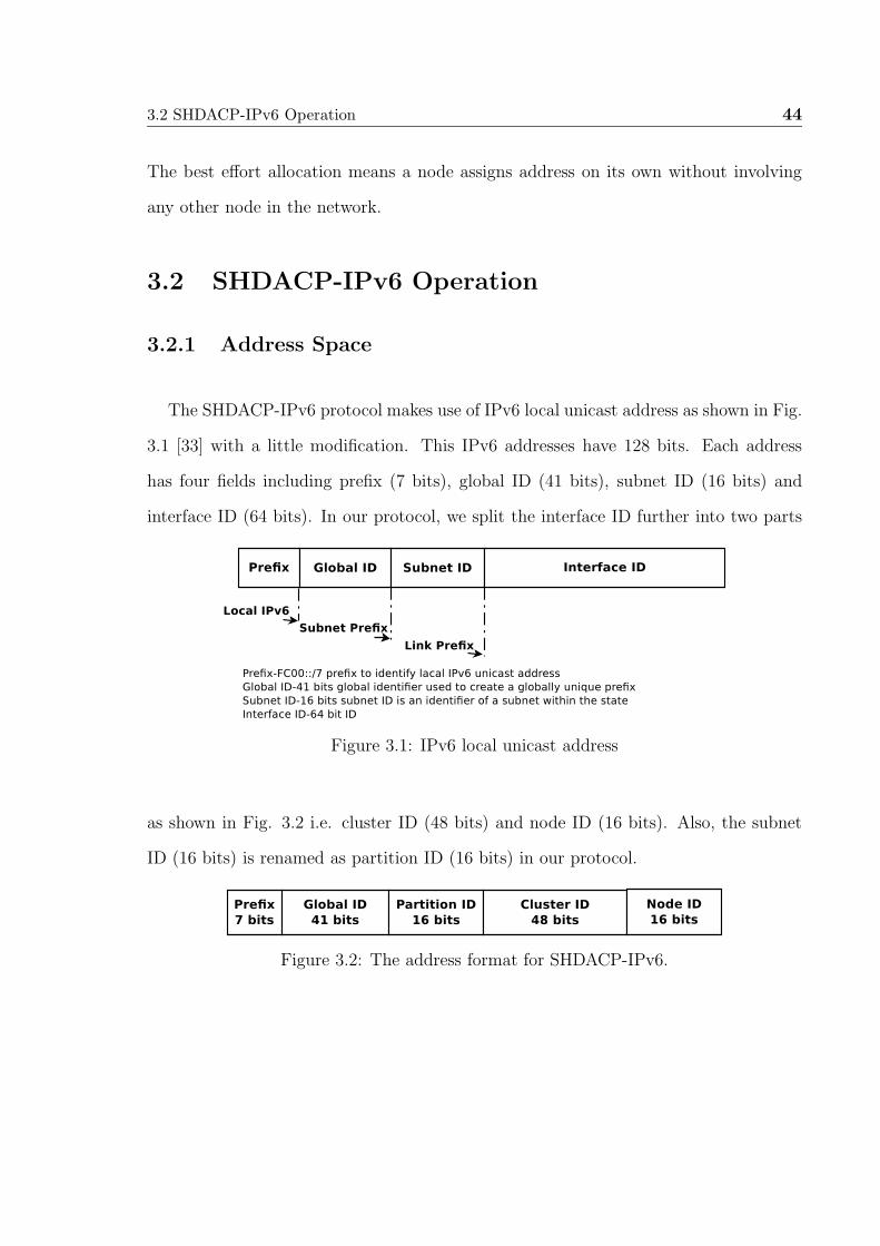
3.2 SHDACP-IPv6 Operation 44
The best effort allocation means a node assigns address on its own without involving
any other node in the network.
3.2 SHDACP-IPv6 Operation
3.2.1 Address Space
The SHDACP-IPv6 protocol makes use of IPv6 local unicast address as shown in Fig.
3.1 [33] with a little modification. This IPv6 addresses have 128 bits. Each address
has four fields including prefix (7 bits), global ID (41 bits), subnet ID (16 bits) and
interface ID (64 bits). In our protocol, we split the interface ID further into two parts
Figure 3.1: IPv6 local unicast address
as shown in Fig. 3.2 i.e. cluster ID (48 bits) and node ID (16 bits). Also, the subnet
ID (16 bits) is renamed as partition ID (16 bits) in our protocol.
Figure 3.2: The address format for SHDACP-IPv6.

3.2 SHDACP-IPv6 Operation 45
3.2.2 Network Formation
When the first node enters in the network, it broadcasts Neighbor Query message in
order to search for neighbors in the network. After broadcasting the Neighbor Query
message, a new node (i.e. requester) will wait for a Neighbor Reply message from
atleast one of the configured nodes. The requester will wait till the expiry of the
Neighbor Reply Timer to receive the Neighbor Reply message. If it does not receive
any Neighbor Reply message before the expiry of the timer, then it rebroadcasts the
Neighbor Query message. The requester repeats this process for a threshold (q) number
of times or till it receives a Neighbor Reply message. If no Neighbor Reply message is
received, then the requester realizes itself to be the only node in the network and
configures itself as a cluster head (CH) by randomly selecting a partition number, a
random cluster number and assigns node id 1 to itself. Now, this CH will participate
in the address allocation for the new nodes arriving in its vicinity. When this CH
receives an address request, then it will allocate the addresses sequentially from node id
2 onwards, while the partition id and cluster id of the addresses allocated will remain
the same as that of the CH. In this protocol, only the CH nodes can allocate the IP
addresses to the incoming nodes. The configured nodes need to store their hop distance
from their respective cluster heads as learnt from time to time. Fig. 3.3 shows the steps
involved in configuring a new node.
When nth node (requester) enters the network, it broadcasts a Neighbor Query mes-
sage. All the configured nodes that receive the Neighbor Query message, will respond
back with a Neighbor Reply message. Each Neighbor Reply message contains copies
of the three fields maintained by the responder node, i.e. the hop distance to its CH,
hmax, and its partition id. Only the nodes whose hop distance is less than hmax hops

3.2 SHDACP-IPv6 Operation 46
Figure 3.3: Steps involved in configuring a new node.
from its respective CH can participate in the address allocation for the requester. The
value of hmax is decided initially when a node becomes a cluster head. When a node is
allocated an address, it will also store hmax of its cluster head as passed to him by the
initiator node. If the requester receives more than one Neighbor Reply messages, then
it will choose a neighbor with the least number of hops to its respective cluster head.

3.2 SHDACP-IPv6 Operation 47
The selected neighbor is then referred to as an initiator. The requester node sends an
Address Request message to the initiator node. The initiator node forwards the same
to its cluster head. When the cluster head receives the Address Request message, then
it chooses an IP address for the requester and sends an Address Allocate message to the
initiator. During this process all the nodes which pass the Address Allocate message
also update their hop distance to CH node record. The initiator then forwards the
Address Allocate message to the requester alongwith the updated hop distance to CH.
The requester will configure itself with the allocated address and becomes a configured
node of the network. If the requester does not receive an Address Allocate message
before the expiry of the Address Allocated timer then it will configure itself as a CH by
choosing the same partition number as present in the Neighbor Reply message and ran-
domly select a cluster number while avoiding those which were identified in the received
Neighbor Reply messages. It then floods the entire network with a New Cluster mes-
sage. Any CH with the same cluster number will reply with a NewCluster NegAck to
the sender of the New Cluster message. If the new CH receives any NewCluster NegAck
then it will randomly choose another different cluster number and again flood the net-
work with the New Cluster message. This protocol is a modified version of the work
reported in [34]. As we are using 48 bits for the cluster ID, the probability of choosing
the same cluster number is very low. In the subsequent section, it is proved that for a
network with 1000 nodes, the probability of the address duplication is of the order of
10−9.
3.2.3 Probability Calculation for the Worst Case Scenario
Let us consider a large scale MANET [35] [36] with n number of nodes such that
100 < n < 1000. The worst case scenario for our protocol is that all the n nodes will

3.2 SHDACP-IPv6 Operation 48
configure themselves as CH and choose a random cluster number. The cluster number is
to be selected using 48 bit address. Let P (A) denote the probability of event A in which
atleast two CH choose the same cluster number, then P (A) denotes the probability that
no two CH choose the same cluster number.
P (A) = 1− P (A). (3.2.1)
Let P (Ei) denote the probability of the event Ei in which newly arriving ith node
chooses a cluster number without any clash. Hence P (Ei) is given as
P (Ei) =248 − i− 1
248. (3.2.2)
The probability P(A) with n nodes in the network can be calculated as
P (A) = P (E1) ∗ P (E2) ∗ ....... ∗ P (En). (3.2.3)
P (A) =248
248∗248 − 1
248∗248 − 2
248∗ .... ∗
248 − n+ 1
248. (3.2.4)
P (A) =(248)n−1 −
�i ∗ (248)n−2 + higher order terms
(248)n−1. (3.2.5)
If we neglect the higher order terms then the above equation can be approximated as
P (A) ∼ 1−n2
249. (3.2.6)
If the network consists of 1000 nodes, then the probability that atleast two CH nodes
choose a same cluster number will be
P (A) =n2
249=
10002
249= 0.000000002. (3.2.7)
Hence, even under the worst case scenario, the probability that atleast two nodes will
select the same cluster number is very low. Moreover, as the size of network increases,
this probability will increase.

3.2 SHDACP-IPv6 Operation 49
3.2.4 Network Partitioning
In MANETs due to random mobility of the mobile nodes, there is a high probability
that network can split into multiple partitions. The network partitioning occurs when
some of the nodes move out of the range of the parent partition and form another
small partition (child partition) as shown in Fig. 3.4 . Most of the existing auto-
Figure 3.4: Network partioning due to nodes mobility
configuration protocols [16] [28] in the literature use different methods to detect the
network partitioning. These protocols involve periodic broadcast of the Hello packet
from each of the nodes in order to keep track of alive nodes in the network. When a Hello
packet is not received by a node from a neighbor listed in local table, the node assumes
that either the node is dead or it has moved away forming its own new partition. This
generates a lot of control overhead in the network.
In our protocol, when a node gets configured then the partition id of that node is
embedded in the IP address. Further if a node moves to a different partition, it will

3.2 SHDACP-IPv6 Operation 50
not change its partition id. In SHDACP-IPv6 protocol, we have not incorporated any
method to detect the network partitioning because all the route entries in the routing
table will have an expiry timer associated with them. These entries will be purged out
from the routing table after the timer expiry. Thus, the entries for the nodes which
move away are purged on their own.
Now, we will discuss the four different cases when a configured node moves to a
different partition. The configured node may be a CH node or a normal node.
3.2.4.1 Case 1
The outgoing node is a normal node and moves to a different partition as shown in
Fig. 3.5. Most likely, this node will not experience any IP address conflict with the
nodes present in that partition. This is because the partition id’s of the two partitions
will be different with a high probability. Even if the partition id’s are same, there
wouldn’t be any address conflict as the uniqueness of the cluster id’s are assured with
a high probability as discussed in the section 3.2.3. This normal node can respond
to the Neighbor Query messages in new partition also. However, it will respond with
the parameters (partition id and cluster id) same as of its original partition, where
it was configured. In case, it is selected as an initiator by the requester, then it will
not be able to provide an address as it has moved away from its CH. It will also
update hop distance from its CH as ∞ in this process. The requester will wait for the
expiry of the Address Allocated Timer to receive an Address Allocated message. If no
Address Allocate message is received, then the requester will configure itself as a cluster
head while using the partition id as told by initiator node.

3.2 SHDACP-IPv6 Operation 51
Figure 3.5: Normal node moves from one partition to the other partition
3.2.4.2 Case 2
The outgoing node is a cluster head node and moves to a different partition as shown
Figure 3.6: Cluster Head node moves from one partition to the other partition
in Fig. 3.6. The CH node can configure the incoming nodes even if it moves to the
other partition. When the CH receives a Neighbor Query message in new partition,
then it will respond with the Neighbor Reply message with its own partition id. The
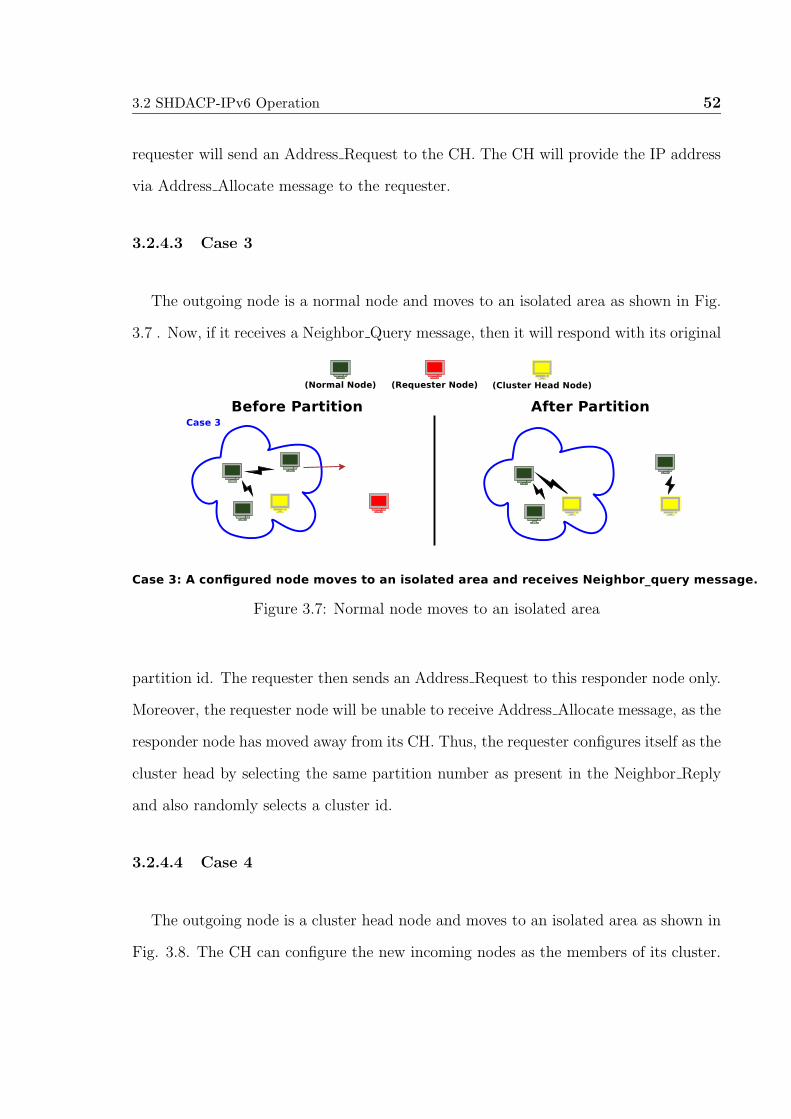
3.2 SHDACP-IPv6 Operation 52
requester will send an Address Request to the CH. The CH will provide the IP address
via Address Allocate message to the requester.
3.2.4.3 Case 3
The outgoing node is a normal node and moves to an isolated area as shown in Fig.
3.7 . Now, if it receives a Neighbor Query message, then it will respond with its original
Figure 3.7: Normal node moves to an isolated area
partition id. The requester then sends an Address Request to this responder node only.
Moreover, the requester node will be unable to receive Address Allocate message, as the
responder node has moved away from its CH. Thus, the requester configures itself as the
cluster head by selecting the same partition number as present in the Neighbor Reply
and also randomly selects a cluster id.
3.2.4.4 Case 4
The outgoing node is a cluster head node and moves to an isolated area as shown in
Fig. 3.8. The CH can configure the new incoming nodes as the members of its cluster.

3.2 SHDACP-IPv6 Operation 53
Figure 3.8: Cluster Head node moves to an isolated area
The CH will provide the IP address (with its original partition id as well as cluster id)
to the requester node.
3.2.5 Network Merging
The merging of different networks is very common in MANETs due to random node
mobility. When merging takes place then two or more small partitions merge together
to form a larger partition. Most of the existing auto-configuration protocols [16] [28]
change the partition number of one of the two networks (involved in merging) to that
of other one. This creates a lot of communication overhead in the network. Moreover,
we need to detect and resolve the address conflicts between the nodes when different
networks merge together. The IP address of all but one of the conflicting nodes need
to be reconfigured. Thus, it increases both the average communication overhead and
average address allocation latency.
In our protocol, when merging is detected, there is no need to change the partition
number of the nodes. The nodes involved in merging (i.e. bridge nodes) will exchange

3.2 SHDACP-IPv6 Operation 54
Figure 3.9: Network Merging
their routing tables so that the two MANETs will be connected. The bridge nodes
will first initiate communication by sending the Exchange Rtable message containing
all its routing table entries. Then, the bridge nodes will flood their respective partitions
with Rtable Flood message containing the routing table entries of the other partition
members addresses. Any node receiving Rtable Flood message creates new routing table
entries for the nodes in the other partition. We have proposed two solutions to detect
the merging of the networks; they are named as weak merging and strong merging.
3.2.5.1 Weak Merging
In this approach, broadcast message transmissions at regular intervals by each node in
the network are not done. Each node after receiving messages from the other nodes will
verify whether these nodes are already present in its routing table. If the sender of the
message is not present in its routing table then the network merging is detected by that
node. Thus, we can reduce the communication overhead in the network substantially.

3.2 SHDACP-IPv6 Operation 55
3.2.5.2 Strong Merging
In strong merging approach, each node in the network periodically broadcasts Hello
messages to its neighbors. After receiving a message from the neighbor node, each node
will check whether the sender of this message is present in its routing table or not. If
the node does not have an entry corresponding to the sender of the message then the
network merging is detected. In addition to the periodic broadcast messages, each node
also uses other kind of messages from the nodes to detect the network merging. Thus,
most of the network merging scenarios can be detected in strong merging as compared
to the weak merging. However, due to the periodic Hello messages, communication
overhead increases.
The proposed SHDACP protocol is a new version of an existing protocol [34] and has
been presented in detail alongwith logical explainations and justifications. It has been
refined in terms of various parameters e.g. the timer associated with messages, address
allocation, and its operation. The results were found to be almost the same as in [34].
3.2.6 Simulation Results
In this section, we have compared the existing protocols such as MANETconf and
AIPAC with our proposed SHDACP-IPv6 (with weak merging) and SHDACP-IPv6
(with strong merging). The metric used for comparison is the average communication
overhead per node, and average address allocation latency. We have used OMNeT++
simulator for performing the simulations of a Mobile Ad-hoc Network (MANET). We
have considered n number of nodes that are moving randomly in a 1000m X 1000m
area. Every node in the network chooses a random initial position, chooses a random
speed and a random direction with which it moves through out the simulation time

3.2 SHDACP-IPv6 Operation 56
period. Random direction and speed is updated periodically after every 1 second. The
inter arrival time of the nodes is uniformly distributed in the range 0-10s. If any node
tries to move out of the simulation area, then it is assumed to be reflected back into
the simulation area by the boundary. Thus, all the nodes will be within the simulation
area during the simulation period. We have performed simulations for 50 runs, each
time with different seeds for random number generators, and an average of all the runs
was taken for obtaining more accurate results. The parameters used for simulation are
given in the table 3.1 :
Table 3.1: Simulation Parameters
Number of Nodes 50 to 500Simulation Area 1000m X 1000mMaximum Speed 5 m/s
Transmission Power 100 milli WattsMinimum Detectable power -54 dBm
Mobility Module update interval 1 secRouting Protocol AODVMAC Protocol 802.11 CSMA/CA
3.2.6.1 Communication Overhead
We have simulated the communication overhead required for configuring a new
node for the existing auto-configuration protocols (AIPAC and MANETconf) and then
we compared the results with our SHDACP-IPv6 protocol. We have observed that
SHDACP-IPv6 with weak merging support generates lowest communication overhead
as shown in Fig. 3.10. The SHDACP-IPv6 protocol with strong merging support per-
forms much better than MANETconf and AIPAC protocols because there is no overhead

3.2 SHDACP-IPv6 Operation 57
50 100 150 200 250 300 350 400 450 5000
50
100
150
200
250
300
350
400
450
500
Number of Nodes
Co
mm
un
icati
on
overh
ead
per
no
de
SHDACP−IPv6 with weak merging
SHDACP−IPv6 with strong merging
MANETconf
AIPAC
Figure 3.10: Average Communication Overhead
for partitioning, also less flooding is required during the address allocation procedure.
The overhead generated in MANETconf is due to the excessive flooding of the initia-
tor request message that is required for seeking permission from all the nodes to grant
an address to the requester. The AIPAC protocol performance degrades with an in-
crease in the number of nodes. This is possibly because of its gradual merging method
and its procedure to deal with the network partitions. As the number of nodes increase,
more nodes get involved in merging and partitioning, hence the overhead generated by
AIPAC protocol is more than that of the MANETconf after reaching a certain network
density.
3.2.6.2 Address Allocation Latency
The address allocation latency is defined as the time taken by a node to get configured
in the network. We have compared different auto-configuration protocols (MANETconf
and AIPAC) with our protocol, on the basis of their average address allocation latencies

3.2 SHDACP-IPv6 Operation 58
as shown in Fig. 3.11. Using the address allocation latency for all the nodes configured
for, we compute the average address allocation latency. We observe that the perfor-
50 100 150 200 250 300 350 400 450 5005
10
15
20
25
30
35
Number of nodes
Ad
dre
ss A
llo
cati
on
Late
ncy p
er
no
de (
in s
eco
nd
s)
SHDACP−IPv6 with weak merging
SHDACP−IPv6 with strong merging
MANETconf
AIPAC
Figure 3.11: Average Address Allocation Latency
mance of SHDACP-IPv6 with strong merging support and SHDACP-IPv6 with weak
merging support is almost the same. The only difference between the strong and the
weak merging support is the transmission of the periodic Hello messages which affects
the average communication overhead but not the average address allocation latency. We
observe that for a fixed number of nodes, the address allocation latency of SHDACP-
IPv6 protocol is less than that of the MANETconf protocol. In MANETconf protocol
[16], the address allocation latency is high as the initiator needs to wait for the responses
from all the nodes before allocating an address to the requester. While in SHDACP-
IPv6 protocol, the cluster head node directly allocates the address, thus reducing the
address allocation latency. In AIPAC protocol [28], it is necessary for an unconfigured
node to be in the neighborhood of the already configured or another unconfigured node,
thus avoiding the formation of single node networks. On the other hand, if the num-
ber of nodes are less, then it becomes difficult for a node to find another node in its

3.2 SHDACP-IPv6 Operation 59
neighborhood. This increases the average address allocation latency. However, as the
number of nodes increase, all such unconfigured isolated nodes are configured, possibly
because the new nodes arrive in their neighborhood. However, we observe that after
reaching a certain network density, the average allocation latency of AIPAC protocol
increases again. This is possibly because of the gradual merging procedure, which re-
quires a node to be reconfigured again. As the number of nodes increase further, the
nodes involved in this gradual merging procedure increase, thus increasing the average
address allocation latency.
3.2.6.3 Comparing SHDACP-IPv6 Strong and Weak Merging Supports
We have already discussed that SHDACP-IPv6 protocol with a strong merging sup-
port is able to detect more merging scenarios in comparison to that of the SHDACP-
50 100 150 200 250 300 350 400 450 50010
20
30
40
50
60
70
80
90
100
Number of nodes
Perc
en
tag
e o
f n
od
es in
vo
lved
in
merg
ing
SHDACP−IPv6 with weak merging
SHDACP−IPv6 with strong merging
Figure 3.12: Comparing merging scenarios detection
IPv6 with a weak merging support because it employs periodic Hello messages. Thus,
there is a trade off between the communication overhead and merging scenario detec-
tion. In simulations, we observe that the percentage of the nodes involved in merging

3.3 SHDACP-IPv4 Operation 60
for SHDACP-IPv6 with strong merging support is much higher than that of the weak
merging support as shown in Fig. 3.12 . However, as the number of nodes increase, the
merging scenario detection in both the versions becomes almost the same.
3.3 SHDACP-IPv4 Operation
3.3.1 Address Space
The proposed SHDACP-IPv4 version deals with IPv4 address space. Here, we have
considered a private IPv4 addresses block (10.0.0.0 - 10.255.255.255) for addressing the
nodes in a MANET. The IPv4 address space of 32 bits is split into four fields i.e. prefix
(8 bits), partition ID (10 bits), cluster ID (10 bits), and node ID (4 bits) as shown in
Fig. 3.13 .
Figure 3.13: Hierarchical Distributive Address Version
In the SHDACP-IPv4 version, each node will maintain a Cluster id table. This table
contains the existing cluster id’s within a partition. This table helps to avoid the cluster
id duplicacy within a partition. The entries in this table are updated on the basis of
the headers in the received messages from the other nodes. When a node receives a
message then it will update its Cluster id table by adding the cluster id of the received
message in its own table if the message is from some node of the same partition. The
address for new nodes are allocated by CH sequentially. In this protocol, each node
will store its hop distance from its respective cluster head. The algorithm by which the
SHDACP-IPv4 works is as follows.
3.3 SHDACP-IPv4 Operation 61
3.3.2 Network Formation
When a new node (i.e. requester) enters the network, it will broadcast Neigh-
bor Query message and will wait for a Neighbor Reply message from the configured
nodes. All the configured nodes that receive the Neighbor Query message, will respond
back with the Neighbor Reply message. The Neighbor Reply message will contain two
fields of the responder node i.e. the hop distance from its cluster head (CH) and its
partition id. In case, the requester does not receive any Neighbor Reply before the
expiry of the timer, then it will rebroadcast the Neighbor Query message. This process
will be repeated for q (threshold) number of times or till it receives Neighbor Reply
message. If the requester does not receive even a single Neighbor Reply message after
q attempts, then it will assume itself to be the only node present in the network and
will configure itself as a cluster head (CH) by randomly selecting a partition number, a
random cluster number and the node id 1. However if the requester receives more than
one Neighbor Reply messages, then it will choose a responder (as initiator) with the
least number of hops from the respective cluster head. The requester node will send an
Address Request message to the selected initiator node. The initiator will forward the
received Address Request to its CH. The CH will choose an IP address for the requester
and send an Address Allocate message to the initiator, which then forwards the same
to the requester. When Address Allocate message is sent, the initiator also updates
the record of hop distance from CH. The requester will then configure itself with the
allocated address and become a configured node of the network. If the requester does
not receive an Address Allocate message before the expiry of Address Allotted timer
then the requester will configure itself as a new CH, by choosing a partition number
as present in one of the earlier received Neighbor Reply messages and randomly select-
ing a cluster id. The new CH will then flood the entire network with a New Cluster

3.3 SHDACP-IPv4 Operation 62
message. Each node will check its Cluster id table, in case a node detects a cluster
id match then it will discard the message. If it is not there in the table, then it is
added to the table. The CH with the same cluster number will respond with a New-
Cluster NegAck to the sender of the New Cluster message. If the new CH receives a
NewCluster NegAck, it will again initiate the address allocation process. The address
duplication of two nodes in this protocol is possible only when the partition number,
cluster number and node id in the cluster of both the nodes are same. If the new CH
receives Address Allocate message for its previous sent Address Request message, then
it will send the Address Reject message back to the CH which has sent Address Allocate
message. The detailed flowchart of SHDACP-IPv4 version is shown in Fig. 3.14 .
3.3.3 Simulation Setup and Results
The simulation setup used for performing simulations on a Mobile Ad-hoc Network
(MANET) using OMNeT++ simulator is same as that in Section 3.2.6.. The parameters
used for simulation are same as given in the Table 3.1.
3.3.3.1 Communication Overhead
The communication overhead refers to the amount of overhead (in terms of number of
messages) required by a node to perform auto-configuration. Here, we have compared
the simulation results of SHDACP-IPv6 and SHDACP-IPv4 with the other existing
protocol in terms of average communication overhead per node. As shown in Fig. 3.15,
if the number of nodes are relatively low (200 nodes), then SHDACP-IPv4 protocol
generates slightly more overhead than the SHDACP-IPv6 [37] protocol because there are
more unconfigured nodes in the network and they keep on transmitting Neighbor Query

3.3 SHDACP-IPv4 Operation 63
Figure 3.14: SHDACP-IPv4 version
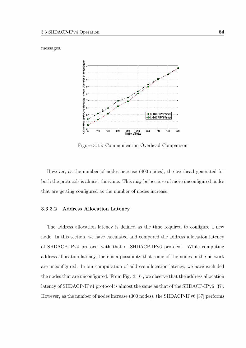
3.3 SHDACP-IPv4 Operation 64
messages.
Figure 3.15: Communication Overhead Comparison
However, as the number of nodes increase (400 nodes), the overhead generated for
both the protocols is almost the same. This may be because of more unconfigured nodes
that are getting configured as the number of nodes increase.
3.3.3.2 Address Allocation Latency
The address allocation latency is defined as the time required to configure a new
node. In this section, we have calculated and compared the address allocation latency
of SHDACP-IPv4 protocol with that of SHDACP-IPv6 protocol. While computing
address allocation latency, there is a possibility that some of the nodes in the network
are unconfigured. In our computation of address allocation latency, we have excluded
the nodes that are unconfigured. From Fig. 3.16 , we observe that the address allocation
latency of SHDACP-IPv4 protocol is almost the same as that of the SHDACP-IPv6 [37].
However, as the number of nodes increase (300 nodes), the SHDACP-IPv6 [37] performs
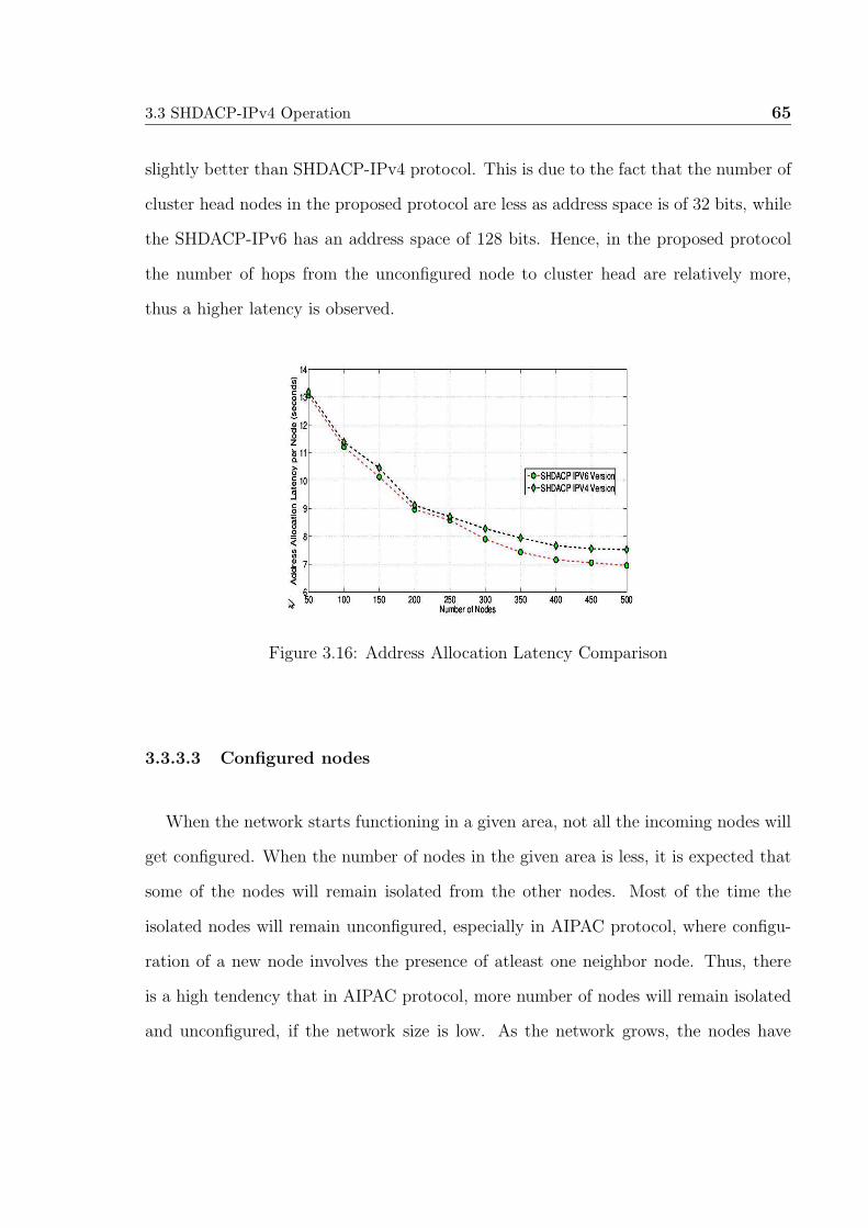
3.3 SHDACP-IPv4 Operation 65
slightly better than SHDACP-IPv4 protocol. This is due to the fact that the number of
cluster head nodes in the proposed protocol are less as address space is of 32 bits, while
the SHDACP-IPv6 has an address space of 128 bits. Hence, in the proposed protocol
the number of hops from the unconfigured node to cluster head are relatively more,
thus a higher latency is observed.
Figure 3.16: Address Allocation Latency Comparison
3.3.3.3 Configured nodes
When the network starts functioning in a given area, not all the incoming nodes will
get configured. When the number of nodes in the given area is less, it is expected that
some of the nodes will remain isolated from the other nodes. Most of the time the
isolated nodes will remain unconfigured, especially in AIPAC protocol, where configu-
ration of a new node involves the presence of atleast one neighbor node. Thus, there
is a high tendency that in AIPAC protocol, more number of nodes will remain isolated
and unconfigured, if the network size is low. As the network grows, the nodes have

3.3 SHDACP-IPv4 Operation 66
higher chances to be in reach of all the other nodes by single hop or multiple hops.
Thus, we expect that a higher fraction of the nodes will get configured as the network
size increases. If there are no arrivals and departures, we expect 100% of the nodes
being configured. Further, due to the new arrivals as well as departures, even for a
fixed population size, we may have less than 100% nodes in a configured state.
In order to verify the above, we have simulated the percentage of configured nodes to
that of the total number of nodes existing in the network. The percentage of configured
nodes in our protocol are then compared with that of AIPAC [26] as shown in Fig 3.17.
When the number of nodes are relatively low (50 nodes), it is found that less than 50 %
of the nodes are configured in AIPAC protocol, whereas in our protocol they are found
to be more than 95 %. This is mainly because AIPAC protocol does not allow the
formation of a single node network. The performance of the AIPAC protocol improves
as the number of nodes increase, while the performance of our protocol is consistent but
slowly reduces at the end. The slight reduction is due to the fact that in our protocol,
address allocation is done by CH only. The number of hops required to obtain address
allocation will depend on the hop distance of the initiator node from the cluster head.
3.3.3.4 Cluster Head Nodes
We have plotted the percentage of nodes that are configured as cluster head to the
total number of nodes existing in the network. As shown in Fig 3.18 , when the number
of nodes in the network is relatively low (50 nodes) then most of the configured nodes
are cluster head nodes because these nodes are scattered throughout the network and
most of them form a single node network. However, as the number of nodes increase, the
percentage of cluster head nodes decrease accordingly. This is mainly because when a
new incoming node enters the dense network, it will be configured by its nearest cluster

3.4 Conclusions 67
Figure 3.17: Percentage of Configured Nodes
head node. In SHDACP-IPv4 protocol, some of the nodes are forced to remain as normal
nodes, if they receive negative acknowledgement message for their New Cluster message.
Thus, for a fixed number of nodes, percentage of cluster head nodes in SHDACP-IPv4
protocol is less than that of the SHDACP-IPv6 protocol.
3.4 Conclusions
In this chapter, we have proposed a scalable hierarchical distributive auto-configuration
protocol (SHDACP) for the mobile adhoc networks. The SHDACP protocol is pro-
posed with two versions i.e. SHDACP-IPv6 and SHDACP-IPv4. In both the versions
of SHDACP, some nodes are termed as cluster heads that are responsible for configuring
the mobile nodes in the network. The main idea of SHDACP is to logically divide the
address space into three fields termed as partition number, cluster number and node
id. The address duplication of the two nodes is possible if the partition number, cluster
number and node id in the cluster of both the nodes are same. The SHDACP-IPv6

3.4 Conclusions 68
Figure 3.18: Percentage of Cluster Head Nodes
protocol has two types of merging support, one with strong merging support and an
another one with a weak merging support.
We have developed a custom simulator using OMNET++ framework for simulating
the protocol. The results obtained through simulation show that SHDACP-IPv6 per-
forms significantly better than the MANETconf and AIPAC protocols. The SHDACP-
IPv6 also reduces the communication overhead in the network substantially, thus mak-
ing it an ideal choice for large scale MANETs. The SHDACP-IPv6 also reduces the
address allocation latency for configuring a new node, as compared to the other proto-
cols in the literature. When the number of nodes are relatively low, then SHDACP-IPv6
with a strong merging support will detect more merging scenarios than the SHDACP-
IPv6 with a weak merging support.
We have also simulated the SHDACP-IPv4 version and result shows that the percent-
age of configured nodes in our protocol is much higher than that of AIPAC [26] protocol,
when the number of nodes are less. Moreover, as the number of nodes increases (50 to

3.4 Conclusions 69
500 nodes), the percentage of configured nodes remains almost the same for SHDACP-
IPv4 irrespective of the number of nodes. The amount of communication overhead in
SHDACP-IPv4 is comparable with that of SHDACP-IPv6 protocol for more number of
nodes (500 nodes), but SHDACP-IPv4 protocol generates slightly more overhead for a
lesser number of nodes. The percentage of cluster heads in the proposed SHDACP-IPv4
protocol is slightly less in comparison to that of SHDACP-IPv6 protocol. The address
allocation latency is almost the same as that of SHDACP-IPv6 protocol, but as the
number of nodes increases (300 nodes), SHDACP-IPv6 version performs slightly better
than the SHDACP-IPv4 protocol.

Chapter 4
Message complexity ofauto-configuration Protocols
In this chapter, we analyze the message complexity1 for configuring a new node using
the existing auto-configuration protocols (MANETconf and AIPAC). The results are
then compared with one of our proposed protocol Scalable Hierarchical Distributive
Auto-configuration protocol (SHDACP) [37][38]. The other objective of this chapter is
to calculate the upper bound on the message overhead required to handle the network
partitions as well as the mergers. These bounds will be very useful in the designing
of different applications in the context of military scenarios and intelligent transport
system (ITS) where mobility is very high and this leads to frequent network partitions
and mergers.
1Amit Munjal and Yatindra Nath Singh “Message Complexity Analysis of Address auto-configuration Protocols in MANETs,” in IEEE TENCON 2014, Bangkok, Thailand, 22-25 Oct2014.

4.1 Message Overhead for configuring a new node 71
4.1 Message Overhead for configuring a new node
In this section, we have calculated the upper bound on the message complexity for
configuring a new node using different auto-configuration protocols such as MANET-
conf and AIPAC. The results are compared with our proposed SHDACP-IPv6 auto-
configuration protocol.
4.2 MANETconf Protocol
4.2.1 Overhead for configuring the new node
Suppose n nodes are already configured in a partition of MANET. When (n+1)st
node enters this partition, it will try to configure itself with the minimum overhead.
Here, we have assumed that all the nodes can reach each other in single hop. In
MANETconf protocol [16], as shown in Fig. 4.1 the new node (i.e. the requester)
first broadcasts Neighbor Query message and will wait for tnq seconds to receive reply
messages from the already configured nodes. However, if it doesn’t recieve reply message
then it will rebroadcast the Neighbor Query message. This process is repeated for q
(threshold) number of times or till it receives reply from any one of the configured nodes
in the network. In the worst case scenario, the requester will receive n Neighbor Reply
messages in its last attempt (q) of Neighbor Query message. The requester will choose
one of the responder nodes as an initiator and send the Requester Request message
to it. The initiator now chooses a new address randomly and floods the network with
the Initiator Request message containing the choosen address. If the initiator receives
even a single negative reply then it will randomly select another address and again
flood the network with the Initiator Request message. In the worst case, an initiator

4.2 MANETconf Protocol 72
Figure 4.1: Steps involved in configuring a (n + 1)st node in MANETconf protocol.
receives all the positive replies in its last attempt (say r). Here, r corresponds to the
maximum number of attempts that an initiator makes, failing which the requester will
send an abort message to the requester. The total number of Positive Ack messages
in the worst case will be r ∗ (n − 2) + 1 and correspondingly the total number of
Negative Ack messages will be (r − 1). After receiving all the positive replies, the
initiator node will allocate the choosen address to the requester node. The initiator node
then updates its Allocated and Allocate pending tables, and also floods the network
with the Address Allot message. Thus, the total number of messages that are required

4.2 MANETconf Protocol 73
to be transmitted in the network for the configuration of (n + 1)st node in the worst
case scenario can be calculated as:
• q Neighbor Query messages,
• n Neighbor Reply messages,
• 1 Requester Request message,
• r Initiator Request messages,
• r *(n - 2) + 1 Positive Ack messages,
• r - 1 Negative reply messages,
• 1 Address Allot messages.
Hence, the upper bound on the communication overhead for configuring the (n+1)st
node in MANETconf is q+(r+1)n+2.
Now, we will calculate the message overhead for configuring a node using MANET-
conf protocol in multihop scenario. Suppose n nodes are configured linearly in a network
as shown in Fig. 4.2. When (n+1)st node enters this partition, it will broadcast Neigh-
bor Query message and will wait for tnq seconds to receive reply messages from the
already configured nodes. In worst case, requester will rebroadcast the Neighbor Query
message for q times. In its last attempt, it will receive reply from one of the configured
node. The requester will choose the responder node as an initiator and send the Re-
quester Request message to it. The initiator now chooses a new address randomly and
floods the network with the Initiator Request message containing the choosen address.
In multihop scenario as shown in Fig. 4.2, if a node receives the Initiator Request, it

4.2 MANETconf Protocol 74
Figure 4.2: Multihop Analysis of configuring (n + 1)st node in MANETconf protocol.
will first check its tables and in case there is an address conflict with the requested
address, it will respond back with a negative reply. On the other hand if a node does
not detect an address conflict then it will simply forward the Initiator Request to its
next hop. In the worst case, an initiator makes r number of attempts and it receives
all the positive replies in its last attempt. Thus, the sum (Sp) of Positive Ack messages
consumed in configuration for this scenario will be calculated as follows.
Sp = [1 + (1 + 2) + (1 + 2 + 3) + ...........(1 + 2 + 3 + .....+ (r − 1))] + r
= [
r−1�
i=1
i ∗ (i+ 1)
2] + r

4.2 MANETconf Protocol 75
= [r−1�
i=1
i2
2+
r−1�
i=1
i
2] + r
=1
2[r−1�
n=1
i2 +r−1�
n=1
i] + r
=1
2[(r − 1)r(2r − 1)
6+
(r − 1)r
2] + r
=(r − 1)r(r + 1)
6+ r
The sum (Sn) of the Negative Acks will be given as follows.
Sn = 1 + 2 + ......... + (r − 1)
Sn =r(r − 1)
2
After receiving all the positive replies, the initiator node will allocate the choosen
address to the requester node. The initiator node then updates its Allocated and
Allocate pending tables, and also floods the network with the Address Allot message.
Thus, the total number of messages that are required to be transmitted in the multi-
hop network for the configuration of (n + 1)st node in the worst case scenario can be
calculated as:
• q Neighbor Query messages,
• 1 Neighbor Reply messages,
• 1 Requester Request message,
•r(r − 1)
2Initiator Request messages,
• Sp Positive Ack messages,
• Sn Negative reply messages,

4.2 MANETconf Protocol 76
• n− 1 Address Allot messages.
Hence, the upper bound on the communication overhead for configuring the (n+1)st
node in linear topology MANETconf is q + n+ r((r2 + 6r − 1)
6).
4.2.2 Partitioning Overhead
In MANETconf, each partition is associated with 2-tuple partition identity. The first
element of partition identity is the lowest IP address in use and second element is the
universal unique identifier (UUID) proposed by the lowest IP address node. Every node
in the partition knows its partition identity. Suppose a network splits into two partitions
parent partition Pp and a child partition Pc as shown in Fig 4.3. Let the number of
nodes with child partition and parent partition are nc and np respectively. The parent
partition is the one that contains the node with the lowest IP address and identity
of this partition will remain unchanged. In this partition, the network partitioning is
detected at the time of the next IP address allocation. During the address allocation, the
initiator node will receive the responses from the np nodes only and hence the initiator
node will figure out that nc nodes left the network. The initiator node will broadcast
nc Address Cleanup messages so that each node in the parent partition should remove
the IP addresses of the nc nodes from their allocated table. Thus, the total number of
Address Cleanup messages in the parent partition will be nc.
In MANETconf, the lowest IP address node in the partition needs to periodically
broadcast a beacon message in order to advertise its presence in the partition. Thus, if
a node fails to receive the beacon message then it detects network partitioning. In child
partition, each of the node will not be able to receive periodic broadcast from the lowest
IP address node. Thus, all the nc nodes will broadcast a partition message. The total

4.2 MANETconf Protocol 77
Figure 4.3: Network Partitioning
number of partition messages in child partition will be nc. When the nodes in child
partition receive the partition messages, they will update their allocated tables. After
updating the tables, each node will compare its IP address with all other IP addresses
in its updated table. If its address is lowest, then it will choose a random partition
number and periodically broadcast a beacon message containing its own IP address and
partition number. The following messages are transmitted in the network when the
partition occurs.
• nc Address Cleanup messages in the parent partition,
• nc partition messages in the child partition.
• 1 partition number configuration message broadcasted in child partition. Hence,
the upper bound on the partition overhead in MANETconf is equal to 2 ∗ nc+1.
4.2.3 Merging Overhead
In MANETconf [16], when two different partitions merge, each node will find other
partition identity during broadcasts. In case the partition identities are different, the
nodes in both the partitions will detect the merger. Each node in both the partitions
will broadcast its allocated tables if not done by some other node. Thus, each node will

4.2 MANETconf Protocol 78
know the allocated tables and partition ids from both the partitions. Fig. 4.4 shows
the merger of two partitions The partition with the higher partition id Ph, changes its
Figure 4.4: Network Merging
partition number to that of the lower partition id Pl. This will be done by all the nodes
belonging to the partition Ph. Let there be nh number of nodes in partition Ph and nl
number of nodes in the partition Pl . As the network is merging, it is quite possible
that there exist x address conflicts. In that case, one of the conflicting node needs to
be reconfigured. The following messages are transmitted in the network when merger
occurs.
• 1 message containing the allocated address in the partition Ph to all the nodes in
the merged partition,
• 1 message containing the allocated address in the partition Pl to all the nodes in
merged partitions,
• configuration overhead x number of nodes.
Hence, the merging overhead, when two partitions merge into a single partition in
MANETconf is 2+(q+(r+1)n+2)x.

4.3 AIPAC protocol 79
4.3 AIPAC protocol
4.3.1 Overhead for configuring the new node
In this protocol [26], when a new node broadcasts Neighbor Query message, it will
wait for tnq seconds to receive a Neighbor Reply message. If a new node does not
receive any Neighbor Reply, then it rebroadcasts the Neighbor Query message. We
first assume single hop network. In the worst case scenario, the new node will transmit
Neighbor Query messages for q (maximum attempts) times and in the last attempt,
it will receive Neighbor Reply messages from s configured nodes in the network. The
requester will select one of nodes as an initiator and forward the initialize request to it.
The initiator will randomly select an address from the available addresses and broadcast
a Search IP packet. If the initiator receives Used IP packet then it will choose another
available address and again broadcast Search IP packet. In the worst case, initiator
will receive Used IP packet for n-1 times. If the initiator does not receive any Used IP
packet, then it will again broadcast the Search IP packet with the same address to get
a confirmation that no reply is coming because the IP address is not in use, and not
due to an error in the wireless channel. The following messages are transmitted in the
network for the configuration of (n+1)st node in the worst case scenario for single hop
network.
• q number of Neighbor Query messages,
• s Neighbor Reply messages,
• 1 Initialize Request message,
• n + 1 number of Search IP packets,

4.3 AIPAC protocol 80
• n− 1 number of Used IP packets, and
• 1 Initialize packet.
Hence, the upper bound on the communication overhead for configuring (n + 1)st
node in AIPAC is q + s +2*n +2.
Now, we will consider a multihop scenario in which n nodes are connected linearly
as shown in Fig 4.5. In the worst case scenario, the requester receives reply in qth
attempt. The requester will select the responder node as its initiator and forwards
the initialize request to it. The initiator will randomly select an address from the
available addresses and broadcast a Search IP packet as shown in Fig 4.5. The Search IP
packet will be transmitted throughout the network. If the initiator does not receive any
Used IP packet, then it will rebroadcast the Search IP packet with same address to get
a confirmation that no reply is coming because of IP address being not in use, but not
due to an error in the wireless channel. In the worst case, the initiator receives Used IP
packet from the (n)th node. It will choose another available address and again broadcast
Search IP packet. Next time, the Used IP packet is generated by (n − 1)st node and
so on. Thus, in this topology, the sum (Ss) of Search IP packets in the network can be
calculated as follows.
Ss = (n+ 1)(n− 1) = n2 − 1
The sum (Su) of corresponding Used IP packets can be calculated as follows
Su =n(n− 1)
2
The following messages are transmitted in the network for the configuration of (n+1)st
node in the worst case scenario.
• q number of SendRequest messages,

4.3 AIPAC protocol 81
• 1 Reply message,
• 1 Initialize Request message,
• Ss number of Search IP messages,
• Su number of Used IP messages, and
• 1 Initialize message.
Hence, the upper bound on the communication overhead for configuring (n + 1)st
node in linear topology AIPAC is q + 2 +3n2 − n
2.
4.3.2 Partitioning Overhead
Each network in AIPAC has a unique identifier (NetID). If some of the links within
the network are broken then it can partition the network into two parts, the parent
partition Pp with np nodes and a child partition Pc with the remaining nodes nc.
Let a node x in the partition Pc with a higher IP address then its corresponding
neighbor y in the partition Pp, detects the partition. Node x floods its partition with a
Route Request message to find y. All the nc − 1 nodes present in child partition (Pc)
will rebroadcast the Route Request message. If no reply is received then node x will
choose a new random NetID and flood the network with a Change NetID message. The
Change NetID message contains the original and new NetID’s of the partition. Each of
the nc − 1 nodes will rebroadcast Change NetID message.
In the worst case scenario, all the nc nodes in Pc detect the partition and broadcast
nc Route Request messages and thereafter nc Change NetID messages. Thus, the total

4.3 AIPAC protocol 82
number of Route Request and Change NetID messages that flow in the child partition
in the worst case will be nc∗nc. When the nodes receive multiple Change NetID message
for the same original NetID, then the highest NetID will be selected as new NetID. The
following messages are transmitted in the network when partition occurs.
• nc ∗ nc Route Request messages,
• nc ∗ nc Change NetID messages.
Hence, the upper bound on the partition overhead when a single hop network splits
into two partitions in AIPAC is equal to 2 n2c .
Consider a network of n nodes that are linearly connected as shown in Fig 4.8. When
any link within the network is broken then it partitions the network into two parts i.e.
the parent partition Pp and the child partition Pc. The parent partition contains the
lowest IP address of the network. In the worst case, the parent partition contains only
the lowest IP address node and remaining n-1 nodes are present in the child partition
as shown in Fig. 4.8. The node in the child partition that detects the partitioning will
broadcast a Route Request message. The Route Request message is broadcasted n-2
times for the considered topology. If no reply is received, then a new random NetID is
choosen by one of the nodes detecting partition and having higher IP address. It floods
the network with a Change NetID message. For network in Fig. 4.8, node 2 in child
partition will detect the partition and thus will broadcast the Change NetID message.
In the worst case scenario, the Change NetID message is broadcasted n-2 times. Thus,
the following messages are broadcasted in the network when partitioning occurs.
• n-2 Route Request messages,
• n-2 Change NetID messages.

4.3 AIPAC protocol 83
Hence, the upper bound on the partition overhead in AIPAC when in a multihop
network only a single node detects the partition, is equal to 2*n-4.
4.3.3 Merging Overhead
The AIPAC protocol [26], uses gradual merging process that reduces the message
overhead for reconfiguring the nodes when two or more networks come close to each
other. The main idea of gradual merging is that if two networks overlap for a certain
period of time, only then nodes need to reconfigure. The process of gradual merging is
based on the neighborhood table maintained at each node. Each node will switchover
to the other network if its neighbors are more in that network. This node needs to
reconfigure in the new network. If nl nodes merge into a single hop network of nh
nodes, then the upper bound on merging overhead in AIPAC is equal to (q + s +2*nh
+2)*nl.
For analysing AIPAC in multihop network, we have considered two linear networks
with number of nodes n1 and n2(> n1) with associated net id as NETID1 and NETID2
respectively. When two networks tend to merge together, then NetID of the higher
number of nodes (n2) will be used for the overall network. Thus, when the two linear
networks merge, then the overall NetID will be NetID2. The number of nodes that will
perform reconfiguration will be n1. Thus, in AIPAC the upper bound on the merging
overhead for multihop network scenario is equal to�n1+n2
n=n2(q+2+
3n2 − n
2). The closed
form expression for the merging overhead is given as follows.
n1+n2�
n=n2
(q + 2+3n2 − n
2) = (q + 2)(n1 + 1) +
(n1 + n2)2(n1 + n2 + 1)
2−
(n2 − 1)2n2
2

4.4 SHDACP Protocol 84
4.4 SHDACP Protocol
4.4.1 Overhead for configuring a new node
Suppose there exist n number of nodes and c number of cluster heads in a MANET.
If n+1st node (requester) enters in the network, it broadcasts Neighbor Query message.
If no reply is received for a duration of tnq seconds, then the requester rebroadcasts the
Neighbor Query message. In the worst case, the requester broadcasts for q attempts
and receives s Neighbor Reply messages in its last attempt. Requester now chooses an
initiator which is least hops away from its cluster head and sends an Address Request
message. The initiator node then forwards the Address Request to its respective CH.
The CH then selects an address and sends an Address Allocate message to the initiator
which forwards the same to the requester. If Address Allocate message is received after
the expiry of the Address Allocate timer then the requester sends an Address Reject
message. The requester then configures itself as the cluster head and floods the network
with a New Cluster message. The communication overhead for configuring (n + 1)st
node in the network for the worst case scenario can be calculated as follows:
• q Neighbor Query messages,
• s Neighbor Reply messages,
• 1 Address Request message,
• 1 Address Allocate message,
• 1 Address Reject message,
• c + 1 New cluster messages,

4.4 SHDACP Protocol 85
• c Newcluster NegAck messages.
Hence, the upper bound on the communication overhead for configuring (n + 1)st
node in SHDACP protocol is equal to q+s+2*c+4.
Fig. 4.10 shows the comparison of the message overhead required to configure a new
node with the increase in the number of nodes for all the three protocols discussed
earlier. We have plotted the message overhead for configuring a new node in single
hop as well as multihop scenarios. The amount of message overhead for configuring a
new node in multihop scenario for AIPAC protocol is more than that for the single hop
scenario. However, in MANETconf the amount of message overhead is more for single
hop scenario than in the multihop scenario. This is because in multihop scenario each
node will forward the initiator request only if it does not find any address conflict with
the requested address.
Fig. 4.11 shows the message overhead with the number of attempts (q) made by the
requester. We found that as the number of attempts made by the requester increase,
the message overhead increases drastically.
4.4.2 Partitioning Overhead
In SHDACP protocol, when a node gets configured then the partition id of that node
is embedded in its IP address. Further, when a node moves to the other partition, it
will not change its partition id. In SHDACP protocol, there is no need for detecting
the network partitioning because all the route entries in the routing table will have
an expiry timer associated with them. These entries will automatically be purged out
after the expiry of timer. Thus, the amount of overhead involved in partitioning for

4.4 SHDACP Protocol 86
SHDACP is zero.
4.4.3 Merging Overhead
Let there be two partitions Pl , Ph in the network with nl , nh nodes respectively.
If the merging of the partitions Pl , Ph is detected, then the merging communication
overhead is calculated as follows.
• nl − 1 Rtable Flood messages in partition Pl,
• nh − 1 Rtable Flood messages in partition Ph,
• 1 Exchange Rtable message by bridge node of Pl,
• 1 Exchange Rtable message by bridge node of Ph.
Hence, the merging overhead incurred when the two partitions merge is nl + nh.
Fig. 4.12 shows the comparison of the message overhead involved in merging of a
single node network with that of the bigger network. The message overhead for AIPAC
(multihop) is maximum as the configuration overhead is maximum in AIPAC (multi
hop).
Fig. 4.13 shows the comparison of the message overhead when a group of nodes
merge with a bigger network. Here, we have considered the size of a bigger network as
100 nodes and the size of the group that merges with this network is varied from 10 to
100 nodes. As expected, the amount of message overhead increases as the size of the
two groups becomes comparable.

4.5 Conclusion 87
4.5 Conclusion
In this chapter, we have calculated the upper bound on the number of messages re-
quired for configuring a new node, for the existing address auto-configuration protocols.
We have also calculated the bound on the message overhead involved in partitioning as
well as in merging and then compared them with our protocol i.e. Scalable Hierarchi-
cal Distributive Auto-configuration protocol (SHDACP). The comparison shows that
SHDACP outperforms MANETconf as well as AIPAC under the worst case scenario.
The amount of overhead required for configuring a new node in SHDACP is lesser in
comparison to that of the MANETconf and AIPAC. Similarly, the amount of merging
overhead is also less than that of the MANETconf and AIPAC. Moreover, our proto-
col works efficiently even after partitioning as no overhead is required to detect the
partitioning.

4.5 Conclusion 88
Figure 4.5: Worst Case Configuration overhead for AIPAC protocol

4.5 Conclusion 89
Figure 4.6: Partitioning of a network into two partitions
Figure 4.7: Partitioning detection via broadcast message
Figure 4.8: Worst Case Partitioning overhead for AIPAC protocol

4.5 Conclusion 90
Figure 4.9: Worst Case Partitioning overhead for AIPAC protocol
0 20 40 60 80 10010
0
101
102
103
104
105
Number of nodes in the network
Me
ss
ag
e o
ve
rhe
ad
fo
r c
on
fig
uri
ng
a n
ew
no
de
MANETconf (single hop)
MANETconf (multi hop)
AIPAC (single hop)
AIPAC (multihop)
SHDACP
Figure 4.10: Message overhead for configuring a new node (with fixed q) with theincrease in number of nodes.

4.5 Conclusion 91
0 20 40 60 80 10010
1
102
103
104
105
106
107
Number of attempts made by requester
Me
ss
ag
e o
ve
rhe
ad
fo
r c
on
fig
uri
ng
a n
ew
no
de
MANETconf (single hop)
MANETconf (multi hop)
AIPAC (single hop)
AIPAC (multihop)
SHDACP
Figure 4.11: Message overhead for configuring a new node with the number of attempts(q) made by requester.
0 200 400 600 800 100010
1
102
103
104
105
106
Number of nodes in the network
Me
ss
ag
e o
ve
rhe
ad
in
sin
gle
no
de
me
rgin
g c
as
e
MANETconf
AIPAC (singlehop)
AIPAC(multihop)
SHDACP
Figure 4.12: Message overhead when n nodes network merges with a single node network

4.5 Conclusion 92
10 20 30 40 50 60 70 80 90 10010
1
102
103
104
105
106
Number of nodes in a group that merges with 100 node network
Me
ss
ag
e o
ve
rhe
ad
in
gro
up
me
rgin
g c
as
e
MANETconf
AIPAC−singlehop
AIPAC−multihop
SHDACP
Figure 4.13: Message overhead when n node network merges with the m nodes network.

Chapter 5
Proposed Stateful AddressAuto-Configuration Protocol forMANETs
In this chapter, we have proposed a new stateful address auto-configuration protocol.
The main aim of this protocol is to allow each node to obtain an unique IP address in
one attempt only. Moreover, this protocol also allows each node to generate a set of
addresses for configuring the new incoming nodes. Further, the proposed protocol also
has an address reclaimation policy that allows the IP address of the outgoing nodes to
be reused by the other nodes with the minimum overhead. The proposed protocol is
simple to implement and also performs efficiently (in terms of latency and overhead)
during mergers as well as partitions.
5.1 Protocol Operation
The purpose of the proposed protocol is to perform the auto-configuration for the
incoming node with a minimum latency. Once the incoming node is configured, it will

5.1 Protocol Operation 94
generate k different IP addresses. The algorithm used for generating these IP addresses
will ensure that these are unused IP addresses. The IP addresses generated by a node
can be used for configuring the other incoming nodes. Thus, each node can have atmost
k child nodes. Each node will keep all the generated k IP addresses in an address table.
This address table is updated whenever an address is allocated by the node. The address
table contains three fields i.e. level indicator and branch indicator to be given to the
child nodes, and status indicating if an address is allocated or not. Fig. 5.1 shows an
address table generated by a node at jth level and ith branch.
Figure 5.1: Address Table of a node at jth level and ith branch
Apart from maintaining the address table, each node also maintains a borrow IP
address table as shown in Fig. 5.2 . The entries of this table are filled by borrowed
address from each of the node which has acquired an IP address generated by this node.
Each node will borrow one address from its child only once after the address allocation.
Thus, the number of entries in the borrow IP address table of a particular node will
also indicate the number of IP addresses that this node has already allocated from its
address table. Each node after performing the address generation procedure will send
its first IP address from its address table to the borrow IP address table of its parent

5.1 Protocol Operation 95
node.
Figure 5.2: Borrow Table of the node at jth level and ith branch
Each IP address in borrow table is also associated with two fields: level identifier and
branch identifier to be allocated to a newly arriving node. Each node also maintains
its own as well as its parent’s records (IP address, level and branch).
Except the root node, all other nodes can allocate k − 1 addresses from the address
table as well as k addresses from the borrow IP address table. Thus, each node can
allocate 2k-1 addresses. This is because each node except the root node needs to forward
its first IP address to its respective parent node. Each configured node will sequentially
allocate the IP addresses from its address table. Once all the IP addresses from the
address table are consumed then the node will start allocating sequentially from the
borrow IP address table.
It is possible that each time an address from the borrow IP address table is allocated
to some new node, an address is borrowed from the new node to replenish the borrow
IP address table, but we have not considered this scenario. Instead, the new node will

5.1 Protocol Operation 96
send one address to the parent node as identified by the level and branch id allotted
to the new node. Thus, once all the addresses from the borrow IP address table are
allocated, the node cannot further assign any IP address. The replenishment of the
borrowed IP address table to the node is not required as it is unlikely that this node
will further receive any query from a new incoming node. Most of the time, the other
nodes around it, who may have been earlier configured by it, will be able to configure
the newly arriving node. This is explained in Fig. 5.3. In this figure, we have considered
Figure 5.3: Example scenario with k = 2
that each node has 2 IP addresses in its address table as well as in the borrow IP address
table (i.e. k = 2 for this case). The node r has allocated an IP address to node a, b
from its address table and c and d from the borrow IP address table. Now, node r does
not have any IP address to be allocated to a new node. As shown in figure, when a new
node sends a Neighbor Query message then the child nodes of node r will be able to
allocate the address. Thus, as more number of nodes join the network, the IP address
allocation is done mostly by the children nodes at the periphery of the network, who
have been configured in the recent past.

5.1 Protocol Operation 97
In this protocol, we are assuming that the network is uniformly growing in all the
directions i.e. the nodes are coming from all the directions at the same rate. Moreover,
each IP address is associated with an IP address timer. Each node except the root
node, needs to renew its IP address before the expiry of the IP address timer. In case,
a parent node does not receive the IP renew request from one of its child nodes before
the expiry of the timer, the parent node assumes that the corresponding child node is
no more the part of the network and the allocated address is reclaimed for further use.
Also, if an IP renew request is not acknowledged, node relinquishes the current address
and initiates the address allocation process as a new node.
5.1.1 Network Formation
When the first node enters the network, it broadcasts Neighbor Query message in
order to search for any possible neighbors in the network. After broadcasting the
Neighbor Query message, the new node (i.e., the requester) will wait till the expiry
of Neighbor Reply timer. By this time, it should receive a Neighbor Reply message
from atleast one of the configured nodes. If the timer expires and it does not receive
any Neighbor Reply message, then it assumes itself to be the only node present in the
network. The new node then initializes itself with the first available address in the
IP address space and becomes the root node. It also maintains the value of its level
identifier and branch identifier as 0. It will then generate k IP addresses at the next
level and these addresses will have the level identifier j as 1 and the branch identifier i
from 0 to k-1 as shown in Fig. 5.4 .
In general, any intermediate node say x which is maintaining its level identifier as j
and the branch identifier as i will generate k IP addresses using the following equation

5.1 Protocol Operation 98
Figure 5.4: Root node generating k IP addresses.
Figure 5.5: Intermediate node x at level j and branch i generating k IP addresses.
(see Fig. 5.5).
IP Address Offset =kj+1 − 1
k − 1+ i ∗ k
tokj+1 − 1
k − 1+ i ∗ k + k − 1. (5.1.1)
All these k addresses are maintained in the address table of the node x. The level

5.1 Protocol Operation 99
identifier and the branch identifier of these IP addresses are as given below.
Level Identifier = j + 1; (5.1.2)
Branch Identifier = i ∗ k + s,
where s = 0, 1, 2, ........, k − 1. (5.1.3)
When nth node enters the network, it will broadcast a Neighbor Query message.
Each of the configured node upon receiving the Neighbor Query message, will respond
back with the Neighbor Reply message. The Neighbor Reply message contains two
parameters of the responding node, i.e. the number of unallocated IP addresses in the
responder’s address table and the number of unallocated IP addresses in the responder’s
borrow address table. If the requester receives more than one Neighbor Reply message,
then it will select one of the responder node as its initiator. The selection criteria
for the initiator node is on the basis of number of available IP addresses with each
of the responder nodes. The requester selects one of the responders as its initiator
based on the maximum available IP addresses with it. If two or more responders
have the maximum number of available IP addresses, then the requester will choose
any one of them randomly. The requester node will then send an Address Request
message to the selected initiator node. The reception of Address Request message by
the responder node will confirm that it is selected as an initiator. Now, the initiator
node will select one of the unallocated IP address from its address table and send the
same in Address Allotted message to the requester. The Address Allotted message
contains the IP address to be used by the requester node, and the level identifier as
well as branch identifier assigned to it. The requester node configures itself with the
allocated IP address. Then, it generates k different IP addresses using equation 5.1.1

5.1 Protocol Operation 100
and forwards the first generated IP address from its address table to the borrow IP
address table of its parent node as identified by the level and branch identifiers. The
parent node updates its borrow address table by storing the first IP address received
from the child nodes. In case, the requester does not receive an Address Allotted
message before the expiry of Address Allotted timer, then the requester will again send
the Address Request message. The requester will retry for a threshold number of times
or till it receives an Address Alloted message. If it fails to receive an Address Allotted
message in all of its attempts, which will happen only if the requesting node is the only
present node in the region, then it will configure itself with the first address available
in the IP address space and maintain its level identifier and branch identifier as 0.
The node will then generate k IP addresses and maintain its address table as discussed
above. Fig. 5.6 shows the formation of hierarchical address tree in this protocol.
Figure 5.6: Hierarchical Tree formation
Once a node is configured, either by an existing node or by itself, it will perform the
following operations.

5.1 Protocol Operation 101
• It will generate k new IP addresses which can be used to configure the other
incoming nodes upon the receipt of the address request. The process of the address
allocation is sequential.
• It will forward first IP address from its address table to the parent node as identi-
fied by level and branch identifier to populate its borrow address table. It may be
noted that when the address is allotted from borrow address table, the initiator
and the parent node are different.
• If all the IP addrsses are consumed then the initiator node will allocate an unused
IP address from its borrow address table.
• When no addresses are available in the address table and borrow address table,
the node will not respond to the Neighbor Query messages.
5.1.2 Address Reclaimation Policy
The address reclaimation policy is defined as the method by which we can detect
and reuse the IP addresses in the network, which were earlier allocated to the nodes
and are no more in the network. The nodes may have left the MANET at some point of
time, due to their mobility or due to the drainage of their battery power. The absence
of a node from the network may result in creation of voids in the hierarchical address
tree. The voids will be created if the outgoing node is a parent node, but not when it
is a leaf node. This is explained with an example tree shown in Fig. 5.7.
Here, some of the nodes (i.e., nodes b, c, e and i) leave the network after the comple-
tion of the auto-configuration process. The nodes b and e are the parent nodes while
the nodes c and i are the leaf nodes. The exit of a leaf node from the hierarchical
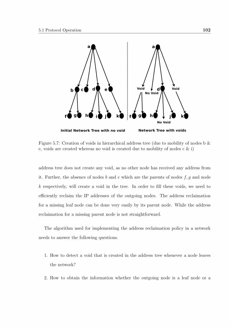
5.1 Protocol Operation 102
Figure 5.7: Creation of voids in hierarchical address tree (due to mobility of nodes b &e, voids are created whereas no void is created due to mobility of nodes c & i)
address tree does not create any void, as no other node has received any address from
it. Further, the absence of nodes b and e which are the parents of nodes f, g and node
k respectively, will create a void in the tree. In order to fill these voids, we need to
efficiently reclaim the IP addresses of the outgoing nodes. The address reclaimation
for a missing leaf node can be done very easily by its parent node. While the address
reclaimation for a missing parent node is not straightforward.
The algorithm used for implementing the address reclaimation policy in a network
needs to answer the following questions.
1. How to detect a void that is created in the address tree whenever a node leaves
the network?
2. How to obtain the information whether the outgoing node is a leaf node or a
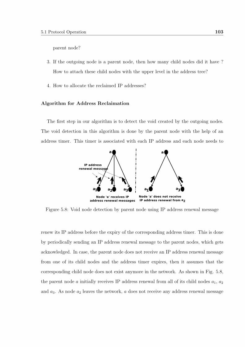
5.1 Protocol Operation 103
parent node?
3. If the outgoing node is a parent node, then how many child nodes did it have ?
How to attach these child nodes with the upper level in the address tree?
4. How to allocate the reclaimed IP addresses?
Algorithm for Address Reclaimation
The first step in our algorithm is to detect the void created by the outgoing nodes.
The void detection in this algorithm is done by the parent node with the help of an
address timer. This timer is associated with each IP address and each node needs to
Figure 5.8: Void node detection by parent node using IP address renewal message
renew its IP address before the expiry of the corresponding address timer. This is done
by periodically sending an IP address renewal message to the parent nodes, which gets
acknowledged. In case, the parent node does not receive an IP address renewal message
from one of its child nodes and the address timer expires, then it assumes that the
corresponding child node does not exist anymore in the network. As shown in Fig. 5.8,
the parent node a initially receives IP address renewal from all of its child nodes a1, a2
and a3. As node a2 leaves the network, a does not receive any address renewal message

5.1 Protocol Operation 104
from a2. Thus, the parent node a detects the void created by node a2 in the tree.
The next step after detection of void is to identify whether the outgoing node is a
leaf node or a parent node. In order to do so, we have introduced a term known as IP
address count. The IP address count of a node is defined as the number of child nodes
that are currently associated with it. In case a node is a leaf node then its IP address
count is 0. Each node will send its IP address count to the parent node periodically
or whenever it allocates an IP address to an incoming node. Fig. 5.9 shows a scenario
where each node is periodically sending its IP address count to its parent node. Here
the nodes a, a1, a2 are parent nodes, while the nodes a11, a21, a22, a23 and a3 are the leaf
nodes.
Figure 5.9: Parent node stores the address count of all its child nodes in an addresscount table.
The parent node maintains the record of the IP address count of all its child nodes in
a separate table known as Address count table. Thus, when a node leaves the network

5.1 Protocol Operation 105
then its parent node can identify from the address count table whether the outgoing
node is a leaf node or a parent node. Now, we will discuss both the cases.
5.1.2.1 Outgoing node is a leaf node
When the parent node identifies that the outgoing node is a leaf node, then the
address reclamation policy is straight forward. This is because the IP address count of
the outgoing node is zero. This means that the outgoing node has not allocated any
IP address before leaving the network. Fig. 5.10 shows the scenario when one of the
leaf node (a3) leaves the network. So, once the parent node detects that one of its child
node whose IP address count is zero, has left the network, then it will change the status
as unallocated for that IP address in its address table. The IP address count table also
gets modified for parent node a. The parent node will then allocate the reclaimed IP
address to any new incoming node.
Figure 5.10: Leaf node moves out of the network

5.1 Protocol Operation 106
5.1.2.2 Outgoing node is not a leaf node
Here, we will consider the case when the outgoing node is not a leaf node such as
node a2 in Fig. 5.9 . When this node leaves the network, then the resulting address
tree gets disconnected as shown in Fig. 5.11 . Here, the child nodes of node a2 i.e.
the nodes a21, a22 and a23 are disconnected from the tree. Now, the parent node of
a2 node i.e. node a needs to connect the child nodes of a2 in the tree. The parent
Figure 5.11: Parent node leaves the network.
node a then checks the IP address count of a2 (which is 3 in the current example)
from its address count table. It then generates the IP addresses of the child nodes of
the missing node i.e. node a will generate a21, a22, a23. This is possible because the
parent node a knows the level indicator and branch indicator of a2. The parent node
a then provides acknowledgements for address renewals, for all the child nodes (a21,
a22, a23) of the outgoing node, till the outgoing node’s IP address is alloted to another

5.1 Protocol Operation 107
new incoming node. Parent node a also now recreates allocated address table using the
received renewal requests. The new node now will take over all the functionalities of
node a2. Fig. 5.12 shows that the parent node a allocates an address a2 to the incoming
node. When the parent node allocates the IP address of the missing node to any new
incoming node, then it also gives the address count as well as allocated address table
associated with that IP address. The new node then generates k IP addresses in its
address table as discussed in our protocol, and marks the status as allocated for the
IP addresses based on the received renewal requests. If it does not receive the address
renewal request from any of the already existing child nodes, then it will change its
status as unallocated.
Figure 5.12: Parent node allocates the reclaimed address (i.e. a2) to new incomingnode.
Thus, the parent node successfully reclaims the IP address with the help of the IP
address count and received renewal requests, when the outgoing child node is not a leaf
node.

5.2 Simulation Results 108
5.2 Simulation Results
In this section, we have simulated and compared our proposed protocol with the
other three existing stateful protocols [16][19][22]. The comparison is made in terms
0 20 40 60 80 100 120 140 160 180 20010
0
101
102
103
Number of nodes
Messag
e O
verh
ead
MANETconf
RSVconf
D2HCP
Proposed
Figure 5.13: Message overhead with number of nodes in the network for initiator at-tempts (i.e. r=2).
of the message overhead for configuring (n + 1)st node with respect to the n number
of nodes. For simulation purpose, we have considered the size of the network growing
from 10 to 200 nodes.
Fig. 5.13 shows a comparison of the proposed protocol with MANETconf, RSVconf
and D2HCP stateful auto-configuration protocols. This figure clearly depicts that for
a lesser number of nodes (20) in the network, the amount of overhead is maximum
for D2HCP and minimum for the proposed protocol. As the number of nodes increase

5.2 Simulation Results 109
(200), the MANETconf protocol consumes maximum amount of overhead, while the
proposed protocol always consumes minimum overhead for configuring (n+1)st node.
0 5 1010
1
102
103
Number of initiator attempts
Me
ss
ag
e o
ve
rhe
ad
MANETconf
RSVconf
D2HCP
Proposed
(a) n=10.
0 5 1010
1
102
103
Number of initiator attempts
Me
ss
ag
e o
ve
rhe
ad
MANETconf
RSVconf
D2HCP
Proposed
(b) n=20.
0 5 1010
1
102
103
Number of initiator attempts
Me
ss
ag
e O
ve
rhe
ad
MANETconf
RSVconf
D2HCP
Proposed
(c) n=50.
0 5 1010
2
103
104
Number of initiator attempts
Me
ss
ag
e o
ve
rhe
ad
MANETconf
RSVconf
D2HCP
Proposed
(d) n=100.
Figure 5.14: Message overhead with number of initiator attempts for different sizenetwork (i.e. n = 10, 20, 50, 100).
Fig. 5.14 show a comparison of message overhead with the number of initiator
attempts for different stateful auto-configuration protocols. The plots shown in 5.14
shows that the amount of message overhead increases with the number of nodes for
different initiator attempts. Our proposed protocol consumes minimal overhead in
comparison to the other protocols.

5.3 Conclusion 110
5.3 Conclusion
This chapter proposes a new stateful address auto-configuration protocol for MANETs.
The proposed protocol is compared with the three existing stateful protocols MANET-
conf, RSVconf and D2HCP. The comparison shows that the proposed protocol requires
minimal message overhead for configuring a new node. Moreover, the proposed protocol
allows the nodes to perform addressing in parllel. The protocol is simple to implement
and also has an address reclaimation policy for an efficient address space utilization.
Chapter 6
Proposed Variant of MANETconfand Message complexity of statefulprotocols
In this chapter, we have proposed an improved variation of auto-configuration pro-
tocol MANETconf1. The communication overhead required for configuring a new node
has been used as performance metric to evaluate the improvement. We have also com-
puted and compared the upper bound on the message complexity [39][40]for configuring
a new node for most of the existing stateful auto-configuration protocols.
6.1 Proposed Variant of MANETconf
In this protocol, each configured node will maintain two tables viz, theAllocated table
and the Allocate pending table. The Allocated table of a node contains all the IP ad-
dresses that are allocated in the network as per the node’s knowledge. TheAllocate pending
table contains those IP addresses for which the address allocation has been initiated
1Amit Munjal and Yatindra Nath Singh “An improved auto-configuration protocol variation byimprovising MANETconf,”IEEE International conference on Advanced networks and Telecommunica-tions systems (ANTS), New Delhi,14-17 Dec 2014.

6.1 Proposed Variant of MANETconf 112
but has not yet been completed.
When a new node (i.e. the requester) wishes to join the network, it will broadcast
Neighbor Query message and will wait to receive the Neighbor Reply message from the
already configured nodes. The requester waits for the expiry of theNeighbor Reply T imer
to receive the responses. If the requester fails to receive the Neighbor Reply message be-
fore the expiry of the Neighbor Reply T imer, then it rebroadcasts theNeighbor Query
message for q (a threshold) times or till it receives the Neighbor Reply message. If the
requester fails to receive the Neighbor Reply message even after q attempts, then it
will assume itself to be the only node in the network and will configure itself with an
IP address.
Figure 6.1: Steps involved in proposed variant of MANETconf protocol for configuringa node.
On the other hand, if the requester receives multiple Neighbor Reply messages, then

6.1 Proposed Variant of MANETconf 113
it will select one of the responders as its initiator. The selection criteria for the initiator
node is based on the signal strength of the received Neighbor Reply message. The
responder with the maximum signal strength will be selected as the initiator node. The
requester node then sends the Requester Request to the selected initiator node. The
initiator node then selects an address (say x), which is not present in any of its tables
(i.e. Allocated table and Allocate pending table) and forwards the Initiator Request
message to all other nodes in the network. When the configured nodes receive the
Initiator Request message, they will check for the address x in their tables. If the
configured node does not detect an address match then it will not respond back to
the initiator with a Positive Ack message. While in original MANETconf protocol,
a Positive Ack is expected from all other nodes before the address allocation is con-
firmed to requester. Further if the configured node detects a match of the address
x in any of its tables, then it will respond with a Negative Ack back to the initia-
tor. Thus, the initiator node will demand the response only from those configured
nodes which have detected an address conflict for the address x in any of their ta-
bles. If the initiator node receives the Negative Ack message before the expiry of the
Initiator Request T imer, then it will again choose another address and repeat the
same for r (i.e. the Initiator Request Retry) number of times. Moreover, if the ini-
tiator receives Negative Ack message in all the r attempts, then it will send an abort
message to the requester. The abort message conveys the requester that it is not pos-
sible for the initiator to configure the requester. The requester will again initiate the
configuration process.

6.1 Proposed Variant of MANETconf 114
6.1.1 Message complexity of auto-configuration Protocols
In this section, we have considered a scenario in which n nodes are already configured
in a MANET. We have calculated the upper bound on the message complexity that is
required to configure (n+1)st node in MANETconf protocol as well as in the proposed
MANETconf variant. The upper bound on message complexity can be defined as the
maximum amount of message overhead that is required in the worst case for a protocol.
We have assumed that all the nodes in the network can communicate with each other
in a single hop.
6.1.1.1 MANETconf
In MANETconf protocol, the upper bound on the message complexity that is required
to configure (n + 1)st node is calculated as:
• q Neighbor Query messages,
• n Neighbor Reply messages,
• 1 Requester Request message,
• r Initiator Request messages,
• r *(n - 2) + 1 Positive Ack messages,
• r - 1 Negative reply messages,
• 1 Address Allot messages.
Hence, the upper bound on the message complexity required for configuring the

6.1 Proposed Variant of MANETconf 115
(n+ 1)st node in MANETconf is q+n+n*r+1.
6.1.1.2 Variant of MANETconf
In the proposed variant of MANETconf protocol, the upper bound on the message
complexity that is required to configure (n+ 1)st node is calculated as :
• q Neighbor Query messages,
• n Neighbor Reply messages,
• 1 Requester Request message,
• r Initiator Request messages,
• 0 Positive Ack messages,
• r - 1 Negative reply messages,
• 1 Address Allot messages.
Hence, the upper bound on the communication overhead for configuring the (n+1)st
node in MANETconf variant is q+n+2*r+1.
6.1.2 Results
In this section, we have shown the comparison of the upper bound on the message
complexity required to configure (n + 1)st node in MANETconf protocol and its pro-
posed variant. The comparison is done on the basis of the worst case message overhead
with an increase in the number of nodes. As the number of nodes increase, the num-

6.1 Proposed Variant of MANETconf 116
0 20 40 60 80 1000
200
400
600
800
1000
1200
Number of nodes
Nu
mb
er
of
messag
es r
eq
uir
ed
MANETconf
Variant of MANETconf
Figure 6.2: Message complexity for MANETconf and proposed variant.
ber of messages required to configure a new node increase many folds in the original
MANETconf. Fig. 6.2 clearly depicts that the message complexity required to configure
a new node reduces drastically in the proposed MANETconf variant.
6.1.3 Conclusion
In this chapter, we have proposed a variant of the MANETconf auto-configuration
protocol that reduces the communication overhead for configuring a new node. We have
calculated the upper bound on the number of messages required for configuring a new
node, for the existing MANETconf as well as the proposed variant. The results clearly
show that the number of messages required to configure a new node is comparatively
less in the proposed variant with respect to the original MANETconf.
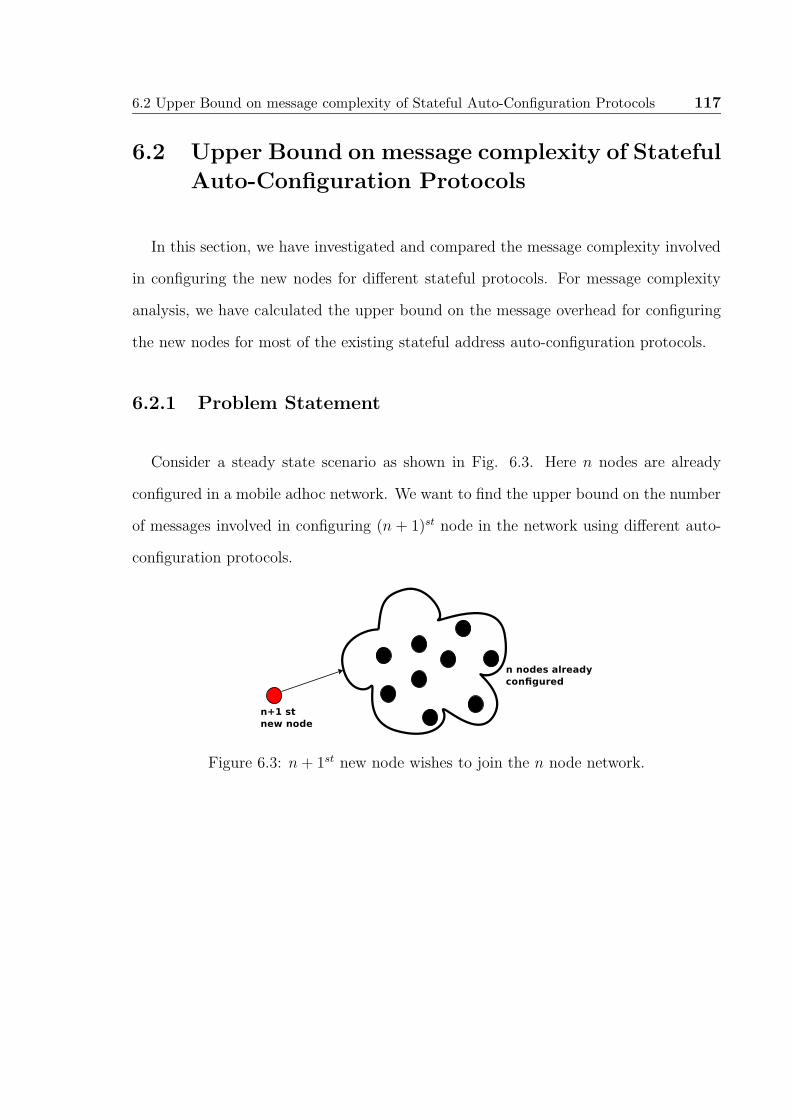
6.2 Upper Bound on message complexity of Stateful Auto-Configuration Protocols 117
6.2 Upper Bound on message complexity of Stateful
Auto-Configuration Protocols
In this section, we have investigated and compared the message complexity involved
in configuring the new nodes for different stateful protocols. For message complexity
analysis, we have calculated the upper bound on the message overhead for configuring
the new nodes for most of the existing stateful address auto-configuration protocols.
6.2.1 Problem Statement
Consider a steady state scenario as shown in Fig. 6.3. Here n nodes are already
configured in a mobile adhoc network. We want to find the upper bound on the number
of messages involved in configuring (n + 1)st node in the network using different auto-
configuration protocols.
Figure 6.3: n+ 1st new node wishes to join the n node network.

6.2 Upper Bound on message complexity of Stateful Auto-Configuration Protocols 118
6.2.2 Stateful Protocols
6.2.2.1 Enhanced Manet Autoconf Protocol (EMAP) [18]
In EMAP [18] protocol, each node generates a pair of the IP addresses (i.e. a tempo-
rary address and a tentative IP address). These addresses are selected from two different
sets of address spaces. The tentative address is the requested address, while the tem-
porary IP address is used only for the time being, till the new node is configured with a
tentative address. The new node first broadcasts DAD REQ message to check for the
Figure 6.4: New node joining a network in EMAP protocol.
availability of the tentative address. If the new node receives DAD REP message before
the expiry of DAD REQ TIMEOUT seconds then it will select another tentative address
(while keeping the same temporary address) and again broadcast DAD REQ message.
As shown in Fig 6.4 , the new node will repeat this process for DAD MAX RETRIES
(q) or till it succeeds. Thus, the upper bound on DAD REQ messages will be q. When
new node receives no DAD REP message within the DAD REQ TIMEOUT seconds
then it assumes that the selected address is unique and will assign the same to its in-
terface. Thus, the upper bound on the message overhead for configuring n + 1st node
in EMAP can be calculated as:

6.2 Upper Bound on message complexity of Stateful Auto-Configuration Protocols 119
• q DAD REQ messages
• q − 1 DAD REP messages.
Thus, the total messages involved =2*q-1.
6.2.2.2 RSVconf [19]
In RSVconf [19] node auto-configuration protocol for MANETs, when a new node
wishes to join the network, it chooses a random address and broadcasts the proxy
request (PREQ) message. If the new node receives more than one proxy reply (PREP)
message, then it will select a proxy whose reply comes first. In the worst case, the
new node receives proxy replies from all the configured nodes (n) as shown in Fig. 6.5.
The new node then sends proxy acknowledgement to the selected proxy. In case the
new node does not receive any reply then it will assign an IP address to itself and will
initialize the network. The selected proxy will select a free IP address from its IP data
Figure 6.5: New node joining a network in RSVconf protocol.

6.2 Upper Bound on message complexity of Stateful Auto-Configuration Protocols 120
base (IPDB) and then broadcast a reservation (RSV) message to get the confirmation
from all the nodes in the network. Each node will check its IPDB and in case a conflict
of IP address is detected then that node will broadcast a response (REP) packet. In
worst case, the proxy receives n − 1 REP messages. Further, if no address conflict is
detected then the proxy will register that IP in its IPDB. The proxy node then sends
an address assignment message that contains the available IP address and the IPDB of
the proxy node. The new node will now forget randomly choosen address and configure
itself with the received information. The total number of messages required to configure
n+ 1st node in the worst case can be calculated as:
• 1 PREQ message,
• n PREP messages,
• 1 Proxy selection message,
• 1 RSV message,
• n− 1 REP message,
• 1 IP address message.
Thus, the total number of messages required to configure n + 1st node in RSVconf is
2*n+3.
6.2.2.3 Logical Hierarchical Addressing (LHA) [20]
In LHA protocol [20] for MANETs, each configured node (Address Agent) can assign
an address to k requester nodes.

6.2 Upper Bound on message complexity of Stateful Auto-Configuration Protocols 121
Figure 6.6: New node joining a network in LHA protocol.
Here, the new node first senses the medium for beacon messages and after listening
the beacon message, it broadcasts an address agent solicitation (AA sol) message. Each
node that receives an AA sol message will respond with AA rep message that contains
the number of currently available free addresses (AfA) with it. In the worst case, the
new node (say n+ 1st) receives r AA rep messages and all the responders have AfA=0
i.e. each of the r responding nodes have consumed their k addresses. It may be noted
in such case (r − 1)(k − 1) + 1 nodes will exist who will have free addresses to be
allocated. Now, the requester will select a responder with the smallest address as its
AA and forward AA sel message to it. The selected AA will broadcast an address
agent address request (AA A req) message. The nodes that listen to this message will
reply with AA A rep message if their AfA>0, otherwise they will further broadcast
AA A req message as shown in Fig. 6.6. If the AA A req message are again received
by nodes with AfA=0, they will further broadcast it. In worst case, AA A req message

6.2 Upper Bound on message complexity of Stateful Auto-Configuration Protocols 122
can be broadcasted r number of times as those many nodes exist with all the addresses
consumed. Thereafter, a node which can allocate an address will surely be found. When
the AA node receives AA A rep message, then it will send AA A sel message to the
selected node. The selected node will send AA conf message to AA. The AA node will
then forward the same to the new node confirming the address allocation.
The number of various messages involved in configuring n + 1st node in LHA are
summarized below.
• 1 AA Sol message,
• r AA rep messages,
• 1 AA sel message,
• r AA A req messages (in worst case),
• s AA A rep message,
• 1 AA A sel message,
• 1 AA conf message.
Thus, the total number of messages required to configure n + 1st node in LHA is
2*r+s+4=2*r+(n-r)+4=r+n+4.
6.2.2.4 Distributed Dynamic Host Configuration Protocol (D2HCP) [22]
When a new node (i.e. the client node) wishes to join the network, it will broadcast
SERVER DISCOVERY message and will wait to receive SERVER OFFER messages
from the configured nodes as shown in Fig. 6.7. If no SERVER OFFER message is

6.2 Upper Bound on message complexity of Stateful Auto-Configuration Protocols 123
received before the expiry of SERVER DISCOVERY TIMER, then the client node re-
broadcasts the SERVER DISCOVERY message for SDISCOVERY MAX RETRY (q)
times or till it receives SERVER OFFER message. In the worst case, the client node
will receive SERVER OFFER messages in its last (qth) attempt. The client node will se-
lect a server from the received SERVER OFFER messages and send a SERVER POLL
message to the selected server. The client node then waits for SERVER POLL TIMER
seconds to receive the IP ASSIGNED message from the selected server. If the client
node fails to receive the IP ASSIGNED message before the expiry of timer, then it
resends the SERVER POLL message for a maximum of SPOLL MAX RETRY (p) or
till IP ASSIGNED message is received. When the server node receives SERVER POLL
message, then it will send IP ASSIGNED message to the client node directly, if free
address is available with the server. If no free address is available with the server
then the server will send IP RANGE REQUEST to the other nodes in the network
and wait for IP RANGE RETURN message. If no IP RANGE RETURN message is
received then the server node resends IP RANGE REQUEST for a maximum RRE-
QUEST MAX RETRY (r) times or till it receives IP RANGE RETURN message.
When the server node receives IP RANGE RETURNmessage then it sends IP ASSIGNED
message to the client node.
The upper bound on the message complexity for configuring n + 1st node when n
nodes are already configured can be calculated as follows:
• q SERVER DISCOVERY messages,
• n SERVER OFFER messages,
• p SERVER POLL messages,

6.2 Upper Bound on message complexity of Stateful Auto-Configuration Protocols 124
Figure 6.7: Client node performing auto-configuration in D2HCP protocol.
• p ∗ r IP RANGE REQUEST messages,
• 1 IP RANGE RETURN message,
• 1 IP ASSIGNED message
Thus, the total number of messages required to configure n + 1st node in D2HCP is
q+n+p*(r+1)+2.
6.2.2.5 One step addressing (OSA)[23]
In this protocol, the new node before joining the network will sense for beacon
messages. When it senses a beacon message, then it will broadcast Add Req message
as shown in Fig. 6.8. If no reply is received, then it will rebroadcast the same for
maximum F times or till it receives an Add Rep message from the existing node. In
the worst case, the n + 1st node will receive Add Rep in its F th attempt. Thus, the
upper bound on the number of Add Req messages will be F . The upper bound on the
Add Rep messages received will be n. The Add rep message contains the number of
free IP addresses available with the node. The new node then selects a responder with

6.2 Upper Bound on message complexity of Stateful Auto-Configuration Protocols 125
maximum number of available IP address as its agent node. It then forwards an Add sel
message to the agent node. The agent node then sends an Add conf message to the new
node. The Add conf message contains the available IP address for configuring the new
node. Thus, the upper bound on the total number of messages involved in configuring
Figure 6.8: New node address auto-configuration in OSA protocol.
n+ 1st node in OSA protocol is summarized below.
• F Add Req messages,
• n Add Rep messages,
• 1 Add Sel message,
• 1 Add conf message.
Thus, the total number of messages required to configure n+1st node in OSA protocol
is F+n+2.
6.2 Upper Bound on message complexity of Stateful Auto-Configuration Protocols 126
6.2.2.6 MANETconf Variant Protocol [41]
The variant of MANETconf protocol aims to reduce the message overhead involved
in configuring a new node. Here, the new node first broadcasts neighbor query mes-
sage and waits for neighbor reply messages from the already configured nodes. If no
response is received before the expiry of neighbor reply timer, then it will rebroadcast
neighbor query message for q (i.e. the threshold) number of times or till it receives the
neighbor reply messages. Thus, the upper bound on the number of neighbor query
messages will be q. Similarly, the upper bound on neighbor reply messages will be n (n
being number of node in the MANET and all of them responding to Neighbor Query
message).
The requester will select a responder node which has maximum signal strength as
its initiator. The requester then sends the requester request to the initiator node. The
initiator node then chooses an address and forwards the initiator request message to
seek permission from the other nodes to grant the choosen address to the requester.
The configured nodes when receive the initiator request message, will check their ta-
bles for an address match and if a match is detected then they will send a negative
response back to the initiator. If no match is deteced then they will not respond. If the
initiator node receives reply before the expiry of initiator request timer, then it will
again choose an address and repeat the process. The process can be repeated r (i.e. the
initiator request retry) number of times and if still address for allocation cannot be
finalized, the failure is indicated. In the worst case, the initiator succeeds in its last at-
tempt (rth). The initiator node will send address allot message to the requester. Thus,
the upper bound for successful address allocation, on the number of initiator request
messages will be r and that of negative responses is r − 1.

6.2 Upper Bound on message complexity of Stateful Auto-Configuration Protocols 127
The the upper bound on the total number of messages involved in configuring n+1st
node in MANETconf variant protocol is summarized below.
• q Neighbor Query messages,
• n Neighbor Reply messages,
• 1 Requester Request message,
• r Initiator Request messages,
• r - 1 Negative reply messages,
• 1 Address Allot messages.
Thus, the total number of messages required to configure n+ 1st node in MANETconf
variant is q+n+2*r+1.
6.2.3 Results
In this section, we have calculated and compared the upper bound on message over-
head complexity for configuring the n+1st node in the network. The message overhead
complexity is plotted with the number of nodes for different auto-configuration pro-
tocols. We have also plotted the message complexity with the increase in number of
requester attempts as well as with number of initiator attempts. The number of nodes
considered for simulation are in the range of 100 to 1000.

6.2 Upper Bound on message complexity of Stateful Auto-Configuration Protocols 128
6.2.3.1 Message overhead with number of nodes
The plots shown in figure 6.9 show the variation of the message overhead with an
increase in the number of nodes (1-100) for different stateful auto-configuration proto-
cols and different requester attempt values. The plots clearly show that the amount
0 20 40 60 80 10010
0
101
102
103
Number of Nodes
Messag
e O
verh
ead
EMAP
MANETconf
MANETconf Variant
RSVconf
LHA
D2HCP
OSA
(a) Requester Attempts q=1.
0 20 40 60 80 10010
0
101
102
103
Number of Nodes
Messag
e O
verh
ead
EMAP
MANETconf
MANETconf Variant
RSVconf
LHA
D2HCP
OSA
(b) Requester Attempts q=2.
0 20 40 60 80 10010
0
101
102
103
Number of nodes
Messag
e O
verh
ead
EMAP
MANETconf
MANETconf Variant
RSVconf
LHA
D2HCP
OSA
(c) Requester Attempts q=5.
0 20 40 60 80 10010
0
101
102
103
Number of nodes
Messag
e O
verh
ead
EMAP
MANETconf
MANETconf Variant
RSVconf
LHA
D2HCP
OSA
(d) Requester Attempts q=10.
Figure 6.9: Message overhead with number of nodes (1-100) in the network for differentrequester attempts (i.e. q = 1, 2, 5, 10).
of message overhead increases with an increase in the number of nodes. The increase
of message overhead is sharp for lesser number of nodes, while for a larger number of
nodes the amount of message overhead tends to saturate for all the auto-configuration

6.2 Upper Bound on message complexity of Stateful Auto-Configuration Protocols 129
protocols. Moreover, the subplots 6.9a, 6.9b, 6.9c and 6.9d are drawn for different val-
ues of requester attempt (q) i.e. 1, 2, 5 and 10. In subplot 6.9a, the amount of message
overhead for EMAP protocol is very low, but in subplot 6.9d, the amount of message
overhead in EMAP increases significantly. This is due to an increase in the number
of requester attempts. The cross-over of curves is due to the fact that when number
of nodes = 0, then arrival of new node means formation of new network. In order to
identify the formation of new network, more messages are needed in LHA and D2HCP
protocols as compared to others.
The plots shown in figure 6.10 show the variation of message overhead with the
number of nodes (1-100) for different stateful auto-configuration protocols. The subplots
6.10a, 6.10b, 6.10c and 6.10d are drawn for different values of initiator attempt (r) i.e.
1, 2, 5 and 10.
The above plots clearly depict that there is an increase in the message overhead of
auto-configuration protocols with the increase in the number of nodes. In subplot 6.10a,
the amount of message overhead for MANETconf protocol is low, but in subplot 6.10d,
the amount of message overhead for MANETconf increases. This is due to the increase
in the number of initiator attempts. The plots also show that the MANETconf protocol
always requires maximum message overhead for configuring a new node.
The plot in figure 6.11 shows the comparison of message overhead involved in con-
figuring a n+ 1st node with the number of nodes for different stateful protocols. Here,
the comparison of message overhead is computed for the higher values of nodes (i.e.
1-1000). The message complexity overhead for configuring n + 1st node increases with
an increase in the number of nodes in the network. The MANETconf protocol re-
quires maximum amount of configuration overhead and it increases many folds with the

6.2 Upper Bound on message complexity of Stateful Auto-Configuration Protocols 130
0 20 40 60 80 10010
0
101
102
103
Number of nodes
Messag
e O
verh
ead
EMAP
MANETconf
MANETconf Variant
RSVconf
LHA
D2HCP
OSA
(a) Initiator Attempts r=1.
0 20 40 60 80 10010
0
101
102
103
Number of nodes
Messag
e O
verh
ead
EMAP
MANETconf
MANETconf Variant
RSVconf
LHA
D2HCP
OSA
(b) Initiator Attempts r=2.
0 20 40 60 80 10010
0
101
102
103
Number of nodes
Messag
e O
verh
ead
EMAP
MANETconf
MANETconf Variant
RSVconf
LHA
D2HCP
OSA
(c) Initiator Attempts r=5.
0 20 40 60 80 10010
0
101
102
103
104
Number of nodes
Messag
e O
verh
ead
EMAP
MANETconf
MANETconf Variant
RSVconf
LHA
D2HCP
OSA
(d) Initiator Attempts r=10.
Figure 6.10: Message overhead with number of nodes (1-100) in the network for differentinitiator attempts (1, 2, 5, 10).
increase in initiator attempts.
6.2.3.2 Message overhead with number of requester attempts
The plot in figure 6.12 shows the comparison of message overhead involved in con-
figuring a n + 1st node with the number of requester attempts for different auto-
configuration protocols. The subplots 6.12a, 6.12b, 6.12c and 6.12d are drawn for
different size of network (n) i.e. 10, 50, 100 and 500. The amount of overhead for all
the auto-configuration protocols increases with the number of nodes.

6.2 Upper Bound on message complexity of Stateful Auto-Configuration Protocols 131
0 200 400 600 800 100010
0
101
102
103
104
105
Number of nodes
Messag
e O
verh
ead
EMAP
MANETconf
MANETconf Variant
RSVconf
LHA
D2HCP
OSA
(a) Initiator Attempts r=10.
0 200 400 600 800 100010
0
101
102
103
104
105
Number of Nodes
Messag
e O
verh
ead
EMAP
MANETconf
MANETconf Variant
RSVconf
LHA
D2HCP
OSA
(b) Initiator Attempts r=20.
0 200 400 600 800 100010
0
101
102
103
104
105
Number of Nodes
Messag
e O
verh
ead
EMAP
MANETconf
MANETconf Variant
RSVconf
LHA
D2HCP
OSA
(c) Initiator Attempts r=50.
0 200 400 600 800 100010
0
101
102
103
104
105
Number of Nodes
Messag
e O
verh
ead
EMAP
MANETconf
MANETconf Variant
RSVconf
LHA
D2HCP
OSA
(d) Initiator Attempts r=100.
Figure 6.11: Message overhead with number of nodes (1-1000) in the network for dif-ferent initiator attempts (10, 20, 50, 100).
6.2.3.3 Message overhead with number of initiator attempts
The plot in figure 6.13 shows the comparison of message overhead involved in config-
uring a n+1st node with the number of initiator attempts for different auto-configuration
protocols. The subplots 6.13a, 6.13b, 6.13c and 6.13d are drawn for different size of net-
work (n) i.e. 10, 50, 100 and 500. The amount of overhead for all the auto-configuration
protocols increases with the number of requester node attempts. Here, we have consid-
ered four different networks with number of nodes 10, 50, 100, 500 respectively.

6.2 Upper Bound on message complexity of Stateful Auto-Configuration Protocols 132
0 2 4 6 8 1010
0
101
102
Number of requester attempts (q)
Messag
e O
verh
ead
EMAP
MANETconf
MANETconf Variant
RSVconf
LHA
D2HCP
OSA
(a) Number of nodes n=10.
0 10 20 30 40 5010
0
101
102
103
Number of requester attempts (q)
Messag
e O
verh
ead
EMAP
MANETconf
MANETconf Variant
RSVconf
LHA
D2HCP
OSA
(b) Number of nodes n=50.
0 20 40 60 80 10010
0
101
102
103
Number of requester attempts (q)
Messag
e O
verh
ead
EMAP
MANETconf
MANETconf Variant
RSVconf
LHA
D2HCP
OSA
(c) Number of nodes n=100.
0 100 200 300 400 50010
0
101
102
103
104
Number of requester attempts (q)
Messag
e O
verh
ead
EMAP
MANETconf
MANETconf Variant
RSVconf
LHA
D2HCP
OSA
(d) Number of nodes n=500.
Figure 6.12: Message overhead with number of requester attempts (q) for different sizenetworks (10, 50, 100, 500 nodes).
6.2.4 Conclusion
In this chapter, we have calculated and compared the upper bound of message over-
head for different stateful auto-configuration protocols in MANETs. The amount of
message overhead involved in configuring a new node is directly related to the number
of nodes in the network, number of requester attempts as well as the number of initiator
attempts. The simulation results show that the MANETconf protocol consumes more

6.2 Upper Bound on message complexity of Stateful Auto-Configuration Protocols 133
0 2 4 6 8 1010
0
101
102
103
Number of initiator attempts (r)
Messag
e O
verh
ead
EMAP
MANETconf
MANETconf Variant
RSVconf
LHA
D2HCP
OSA
(a) Number of nodes n=10.
0 2 4 6 8 1010
0
101
102
103
Number of initiator attempts (r)
Messag
e O
verh
ead
EMAP
MANETconf
MANETconf Variant
RSVconf
LHA
D2HCP
OSA
(b) Number of nodes n=50.
0 2 4 6 8 1010
0
101
102
103
104
Number of initiator attempts (r)
Messag
e O
verh
ead
EMAP
MANETconf
MANETconf Variant
RSVconf
LHA
D2HCP
OSA
(c) Number of nodes n=100.
0 2 4 6 8 1010
0
101
102
103
104
Number of Initiator attempts (r)
Messag
e O
verh
ead
EMAP
MANETconf
MANETconf Variant
RSVconf
LHA
D2HCP
OSA
(d) Number of nodes n=500.
Figure 6.13: Message overhead with number of requester attempts (q) for different sizenetworks (10, 50, 100, 500 nodes).
messages for configuring a new node whereas the EMAP protocol consumes least mes-
sage overhead out of all the protocols discussed in this chapter. The EMAP protocol
on the other hand does not have any partition and merger detection scheme. Thus,
EMAP protocol is not suitable for high mobility scenarios. Our future work is focussed
on the message complexity involved in detecting the partitions as well as the mergers
that happen frequently in MANETs.

Chapter 7
Conclusions and Future Work
In the thesis, we have focussed on one of the most challenging issues in mobile
adhoc networks i.e. auto-configuration of mobile nodes. The auto-configuration is
defined as a process of automatically assigning the IP addresses to every node in the
network, so that each new node can communicate with the other configured nodes via
single hop or multihop wireless links. In other wireless netwoks, the configuration of
mobile nodes is done by a centralized server such as dynamic host configuration protocol
(DHCP) servers. However in MANETs, no such centralized server exists to perform the
configuration of the mobile nodes.
Another challenge in MANETs is that the nodes are mobile, so they will leave or
join the network on their own. This results in frequent network partitions and merg-
ers. So, there is a possibility of duplicate IP addresses to be present in the network
after a merger takes place. Thus, to maintain the uniqueness of IP addresses at the
time of mergers and splits is also challenging. In order to provide the solution for
the above challenges in MANETs, we have proposed stateless and stateful address
auto-configuration protocols. In stateless auto-configuration protocol, no node is main-
taining an information regarding the existing IP addresses used within the network.

135
The proposed stateless auto-configuration protocol is named as Scalable Hierarchical
Distributive Auto-Configuration Protocol (SHDACP). We have proposed two different
versions of SHDACP protocol as mentioned below:
• SHDACP-IPv6
• SHDACP-IPv4
The SHDACP-IPv6 version deals with IPv6 address space for assigning addresses to the
mobile nodes in the network. While the SHDACP-IPv4 version deals with IPv4 address
space. The main idea of both the versions is to logically divide the address space into
three fields: partition number, cluster number and node id. In both the versions, we
have cluster head nodes that are responsible for configuring the mobile nodes in the
network. The main objective of both the versions is to provide an unique IP address to
each node with a minimum message overhead as well as with minimum latency.
The other proposed protocol is stateful address auto-configuration protocol for MANETs.
In stateful approach, each node will maintain the tables corresponding to the IP ad-
dresses of the other nodes. Here, in the proposed protocol, each configured node gener-
ates a set of unique IP addresses and reserves them in its address table. This protocol
also has a borrowing mechanism that allows each node to borrow an IP address from
the node whom it has provided an address. The borrowed IP addresses are stored in
a borrow address table. Moreover, this protocol also allows addresses of the outgoing
nodes to be reclaimed. The address reclaimation policy allows the available address
space to be efficiently utilized.
We have also proposed an improved variation of the existing stateful auto-configuration
protocol MANETconf. The communication overhead required for configuring a new

136
node has been used as performance metric to evaluate the improvement.
Apart from this, we have also calculated and compared the message complexity
required for configuring a new node, for the existing address auto-configuration protocols
with our proposed protocols. The message complexity required to handle network
partition and mergers is also computed. The result shows that our protocol SHDACP
outperforms MANETconf as well as AIPAC under the worst case scenario. Moreover,
our protocol works efficiently even after partitioning as no overhead is required to detect
the partitioning.
We have also computed the upper bound of message overhead required for different
stateful auto-configuration protocols. The simulation results show that the MANET-
conf protocol consumes more messages for configuring a new node whereas the EMAP
protocol consumes least message overhead out of all the protocols discussed in this chap-
ter. The EMAP protocol on the other hand does not have any partition and merger
detection scheme. Thus, EMAP protocol is not suitable for high mobility scenarios.
Future Work
• In stateful auto-configuration protocols, the size of the table depends on the num-
ber of configured nodes. Thus, with an increase in network size, the size of table
at each node increases gradually. Thus, we need to design some protocols that
take care of the memory constraint at each node.
• Time complexity for configuring a node is yet to be computed.
• Message Complexity for detecting mergers and partitions needs to be analyzed.

Bibliography
[1] R. Ramanathan and J. Redi, “A brief overview of ad hoc networks: challenges and
directions,” IEEE communications Magazine, vol. 40, no. 5, pp. 20–22, 2002.
[2] R. Droms, “Dynamic host configuration protocol,” 1997.
[3] L. J. Garcıa Villalba, J. Garcıa Matesanz, A. L. Sandoval Orozco, and J. D.
Marquez Dıaz, “Auto-configuration protocols in mobile ad hoc networks,” Sen-
sors, vol. 11, no. 4, pp. 3652–3666, 2011.
[4] H. Zhou and M. W. Mutka, Review of Autoconfiguration for MANETs. INTECH
Open Access Publisher, 2012.
[5] N. I. C. Wangi, R. V. Prasad, M. Jacobsson, and I. Niemegeers, “Address au-
toconfiguration in wireless ad hoc networks: Protocols and techniques,” Wireless
Communications, IEEE, vol. 15, no. 1, pp. 70–80, 2008.
[6] S. Ahn, N. Kim, W. Kim, and Y. Lee, “A comparison study of address autocon-
figuration schemes for mobile ad hoc network.” in International Conference on
Wireless Networks, 2004, pp. 52–58.
[7] X. Wang and H. Qian, “An ipv6 address configuration scheme for wireless sensor
networks,” Computer Standards & Interfaces, vol. 34, no. 3, pp. 334–341, 2012.

BIBLIOGRAPHY 138
[8] P. Pongpaibool, K. Na Ayutaya, K. Kanchanasut, and H. Tazaki, “Rapid ipv6
address autoconfiguration for heterogeneous mobile technologies,” in ITS Telecom-
munications, 2008. ITST 2008. 8th International Conference on. IEEE, 2008, pp.
234–239.
[9] S. R. Hussain, S. Saha, and A. Rahman, “An efficient and scalable address autocon-
figuration in mobile ad hoc networks,” in Ad-Hoc, Mobile and Wireless Networks.
Springer, 2009, pp. 152–165.
[10] J.-P. Sheu, S.-C. Tu, and L.-H. Chan, “A distributed ip address assignment scheme
in ad hoc networks,” International Journal of Ad Hoc and Ubiquitous Computing,
vol. 3, no. 1, pp. 10–20, 2008.
[11] K. Weniger, “Pacman: Passive autoconfiguration for mobile ad hoc networks,”
Selected Areas in Communications, IEEE Journal on, vol. 23, no. 3, pp. 507–519,
2005.
[12] S. R. Hussain, S. Saha, and A. Rahman, “Saaman: scalable address autoconfigu-
ration in mobile ad hoc networks,” Journal of Network and Systems Management,
vol. 19, no. 3, pp. 394–426, 2011.
[13] L. G. Villalba, A. S. Orozco, J. G. Matesanz, and T.-H. Kim, “E-d2hcp: enhanced
distributed dynamic host configuration protocol,” Computing, vol. 96, no. 9, pp.
777–791, 2014.
[14] M. R. Thoppian and R. Prakash, “A distributed protocol for dynamic address
assignment in mobile ad hoc networks,” Mobile Computing, IEEE Transactions
on, vol. 5, no. 1, pp. 4–19, 2006.

BIBLIOGRAPHY 139
[15] C. Bernardos, M. Calderon, and H. Moustafa, “Survey of ip address autoconfig-
uration mechanisms for manets,” IETF, draft-bernardosmanetautoconf-survey-05.
txt (work-in-progress).(June 2010), 2005.
[16] S. Nesargi and R. Prakash, “Manetconf: Configuration of hosts in a mobile ad hoc
network,” in INFOCOM 2002. Twenty-First Annual Joint Conference of the IEEE
Computer and Communications Societies. Proceedings. IEEE, vol. 2. IEEE, 2002,
pp. 1059–1068.
[17] H. Zhou, L. M. Ni, and M. W. Mutka, “Prophet address allocation for large scale
manets,” Ad Hoc Networks, vol. 1, no. 4, pp. 423–434, 2003.
[18] F. Ros, P. Ruiz, and C. E. Perkins, “Extensible manet auto-configuration proto-
col (emap),” Internet Draft; Available online: http://tools.ietf.org/html/draft-ros-
autoconf-emap-02 Mar, 2006.
[19] R. Bredy, T. Osafune, and M. Lenardi, “Rsvconf: Node autoconfiguration for
manets,” in ITS Telecommunications Proceedings, 2006 6th International Confer-
ence on. IEEE, 2006, pp. 650–653.
[20] A. Yousef, H. Al-Mahdi, A. Mitschele-Thiel et al., “Lha: logical hierarchical ad-
dressing protocol for mobile ad-hoc networks,” in Proceedings of the 2nd ACM
workshop on Performance monitoring and measurement of heterogeneous wireless
and wired networks. ACM, 2007, pp. 96–99.
[21] A. Yousef, A. Diab, and A. Mitschele-Thiel, “Performance evaluation of stateful
address auto-configuration protocols in ad hoc networks,” in Wireless Days (WD),
2009 2nd IFIP. IEEE, 2009, pp. 1–6.

BIBLIOGRAPHY 140
[22] L. J. Garcıa Villalba, J. G. Matesanz, A. L. Sandoval Orozco, and J. D.
Marquez Dıaz, “Distributed dynamic host configuration protocol (d2hcp),” Sen-
sors, vol. 11, no. 4, pp. 4438–4461, 2011.
[23] H. Al-Mahdi, H. Nassar, and S. El-Aziz, “Performance analysis of an autocon-
figuration addressing protocol for ad hoc networks,” Journal of Computer and
Communications, vol. 2013, 2013.
[24] C. Perkins, “Ip address autoconfiguration for ad hoc networks,” IETF draft-ietf-
manet-autoconf-01. txt, 2001.
[25] N. Kim, S. Ahn, and Y. Lee, “Arod: An address autoconfiguration with address
reservation and optimistic duplicated address detection for mobile ad hoc net-
works,” Computer Communications, vol. 30, no. 8, pp. 1913–1925, 2007.
[26] M. Fazio, M. Villari, and A. Puliafito, “Aipac: Automatic ip address configuration
in mobile ad hoc networks,” Computer communications, vol. 29, no. 8, pp. 1189–
1200, 2006.
[27] L. Li, Y. Cai, X. Xu, and Y. Li, “Agent-based passive autoconfiguration for large
scale manets,” Wireless Personal Communications, vol. 43, no. 4, pp. 1741–1749,
2007.
[28] M. Fazio, M. Villari, and A. Puliafito, “Ip address autoconfiguration in ad hoc net-
works: Design, implementation and measurements,” Computer Networks, vol. 50,
no. 7, pp. 898–920, 2006.
[29] K. Weniger and M. Zitterbart, “Ipv6 autoconfiguration in large scale mobile ad-
hoc networks,” in Proceedings of European wireless, vol. 1. Citeseer, 2002, pp.
142–148.
BIBLIOGRAPHY 141
[30] T. Narten, S. Thomson, and T. Jinmei, “Ipv6 stateless address autoconfiguration,”
2007.
[31] M. Grajzer, T. Zernicki, and M. Glkabowski, “Nd++–an extended ipv6 neighbor
discovery protocol for enhanced stateless address autoconfiguration in manets,”
International Journal of Communication Systems, vol. 27, no. 10, pp. 2269–2288,
2014.
[32] M. Mohsin and R. Prakash, “Ip address assignment in a mobile ad hoc network,”
in MILCOM 2002. Proceedings, vol. 2. IEEE, 2002, pp. 856–861.
[33] R. M. Hinden and B. Haberman, “Unique local ipv6 unicast addresses,” 2005.
[34] A. Phaneendra, Y. N. Singh, and A. Roy, “Scalable hierarchical distributive auto
configuration protocol for stand alone mobile ad hoc networks,” 2012.
[35] S. Basagni, M. Conti, S. Giordano, and I. Stojmenovic, Mobile ad hoc networking.
John Wiley & Sons, 2004.
[36] I. Chlamtac, M. Conti, and J. J.-N. Liu, “Mobile ad hoc networking: imperatives
and challenges,” Ad hoc networks, vol. 1, no. 1, pp. 13–64, 2003.
[37] A. Munjal, Y. N. Singh, A. Phaneendra, and A. Roy, “Scalable hierarchical dis-
tributive auto-configuration protocol for manets,” in Signal-Image Technology &
Internet-Based Systems (SITIS), 2013 International Conference on. IEEE, 2013,
pp. 699–705.
[38] A. Munjal, Y. N. Singh, A. K. Phaneendra, and A. Roy, “Ipv4 based hierarchical
distributive auto-configuration protocol for manets,” in TENCON 2014-2014 IEEE
Region 10 Conference. IEEE, 2014, pp. 1–6.

BIBLIOGRAPHY 142
[39] S.-C. Kim and J.-M. Chung, “Message complexity analysis of mobile ad hoc net-
work address autoconfiguration protocols,” Mobile Computing, IEEE Transactions
on, vol. 7, no. 3, pp. 358–371, 2008.
[40] S.-C. kim and J.-M. Chung, “Scalability analysis of stateful and stateless manet
address auto-configuration protocols,” in ICT Convergence (ICTC), 2013 Interna-
tional Conference on. IEEE, 2013, pp. 408–409.
[41] A. Munjal and Y. N. Singh, “An improved autoconfiguration protocol variation by
improvising manetconf,” in ANTS 2014. IEEE, 2014.

List of PublicationsInternational Conferences:
1. Amit Munjal and Yatindra Nath Singh, “An improved auto-configuration proto-
col variation by improvising MANETconf,” IEEE ANTS 2014, New Delhi, 14-17
Dec 2014.
2. Amit Munjal and Yatindra Nath Singh, “Message Complexity Analysis of Ad-
dress Auto-Configuration Protocols in MANETs,” in IEEE TENCON 2014,
Bangkok, Thailand., 22-25 Oct 2014.
3. Amit Munjal, Yatindra Nath Singh, AKrishna Phaneendra and A. Roy “IPv4
based Hierarchical Distributive Auto-Configuration Protocol for MANETs,” in
IEEE TENCON 2014, Bangkok, Thailand., 22-25 Oct 2014.
4. Amit Munjal, Yatindra Nath Singh, AKrishna Phaneendra and A. Roy “Scal-
able Hierarchical Distributive Auto-Configuration Protocol for MANET’s,” In-
ternational Conference on Signal-Image Technology and Internet-Based Systems
(SITIS), Kyoto, Japan 2013, pp. 699-705, doi:10.1109/SITIS.2013.114, 2-5 Dec
2013.
National Conferences:
5. Amit Munjal, Rajiv Tripathi and Yatindra Nath Singh, “Balancing Energy Con-
sumption Using Cluster Based Approach in Wireless Sensor Network,” NCC2014,
IIT Kanpur, 28 Feb-02 Mar 2014.

LIST OF PUBLICATIONS 144
6. Amit Munjal, Anurag Singh, Yatindra Nath Singh, “Using Complex Network
in Wireless Sensor Networks,” Proc. ICEIT Conference on Advances in Mobile
Communications, Networking and Computing, New Delhi, 27-28 Sept 2013.
Papers accepted in Journals:
7. Amit Munjal and Yatindra Nath Singh, “Review of stateful auto-configuration
protocols” Available online at http://dx.doi.org/10.1016/j.adhoc.2015.05.012, Jour-
nal of Adhoc networks, Elseiver.
Papers under review:
8. Amit Munjal and Yatindra Nath Singh, “A Stateful Address Auto-Configuration
Protocol for MANETs,” Journal of Adhoc networks, Elseiver.
9. Amit Munjal and Yatindra Nath Singh, “Upper bound on message complex-
ity of stateful auto-configuration protocols,” Journal of Network and Computer
Applications, Elseiver.
10. Amit Munjal and Yatindra Nath Singh, “Stateless Address Auto-configuration
Protocols in MANETs: A Study,” Journal of Adhoc networks, Elseiver.
Top Related