


Languages
Pages
Legal


Acknowledgments
The Mexico Emissions Inventory Program Advanced Training Workbook was the result of effortsby several participants. The Binational Advisory Committee (BAC) guided the development ofthese manuals. The members of the BAC were:
Dr. John R. Holmes, State of California Air Resources BoardMr. William B. Kuykendal, U.S. Environmental Protection AgencyMr. Gary Neuroth, Arizona Department of Environmental QualityDr. Victor Hugo Páramo, Instituto Nacional de EcologíaMr. Gerardo Rios, U.S. Environmental Protection AgencyMr. Carl Snow, Texas Natural Resource Conservation Commission
The Western Governors’ Association (WGA) was the lead agency for this project. Mr. John T.Leary was the WGA Project Manager. Funding for the development of the workbook wasreceived from the United States Environmental Protection Agency (U.S. EPA). RadianInternational prepared the workbook under the guidance of the BAC and WGA participants.

RCN 670-017-52-02
MEXICO EMISSIONS INVENTORY PROGRAMADVANCED TRAINING WORKBOOK
FINAL
Prepared for:
Western Governors’ AssociationDenver, Colorado
and
Binational Advisory Committee
Prepared by:
Radian International LLC10389 Old Placerville Road
Sacramento, CA 95827
September 1997

Mexico Emissions Inventory ProgramFinal Workbook - September 1997 i
TABLE OF CONTENTS
Page
Introduction . . . . . . . . . . . . . . . . . . . . . . . . . . . . . . . . . . . . . . . . . . . . . . . . . . . . . . . . . . . . . . . 1
Example 1 Stationary Internal Combustion Engines . . . . . . . . . . . . . . . . . . . . . . . . . . . . . . . . 1-1Example 1 Stationary Internal Combustion Engines - Supplemental Information . . . . . . . . . . 1-6
Example 2a External Combustion Devices - Fuel Allocation . . . . . . . . . . . . . . . . . . . . . . . . . 2-1Example 2b External Combustion Devices - Emission Factors . . . . . . . . . . . . . . . . . . . . . . . . 2-4Example 2c External Combustion Devices - Other Estimating Techniques . . . . . . . . . . . . . . . 2-6
Example 3 Residential Fuel Combustion . . . . . . . . . . . . . . . . . . . . . . . . . . . . . . . . . . . . . . . . 3-1
Example 4 Gasoline Distribution System . . . . . . . . . . . . . . . . . . . . . . . . . . . . . . . . . . . . . . . . 4-1Example 4a Aboveground Bulk Storage Tank . . . . . . . . . . . . . . . . . . . . . . . . . . . . . . . . . . . . 4-3Example 4a - Supplemental Information Estimating Individual Species . . . . . . . . . . . . . . . . 4-12Example 4a - Supplemental Information Comparison of Raoult’s Law with Other Methods . . . . . . . . . . . . . . . . . . . . . . . . . . . . . . . . . . . . . . . . . 4-16Example 4b Fugitive (Equipment Leak) Emissions . . . . . . . . . . . . . . . . . . . . . . . . . . . . . . . . 4-18Example 4c Tank Truck Loading Emissions . . . . . . . . . . . . . . . . . . . . . . . . . . . . . . . . . . . . . 4-23Example 4d Tank Truck Transit Emissions . . . . . . . . . . . . . . . . . . . . . . . . . . . . . . . . . . . . . 4-28Example 4e Underground Tank Filling Emissions . . . . . . . . . . . . . . . . . . . . . . . . . . . . . . . . 4-31Example 4f Underground Tank Breathing Emissions . . . . . . . . . . . . . . . . . . . . . . . . . . . . . . 4-34Example 4g Vehicle Refueling Emissions . . . . . . . . . . . . . . . . . . . . . . . . . . . . . . . . . . . . . . . 4-36Example 4 - Summary . . . . . . . . . . . . . . . . . . . . . . . . . . . . . . . . . . . . . . . . . . . . . . . . . . . . . 4-39
Example 5a Solvent Evaporation - Degreasing . . . . . . . . . . . . . . . . . . . . . . . . . . . . . . . . . . . . 5-1Example 5b Solvent Evaporation - Surface Coating . . . . . . . . . . . . . . . . . . . . . . . . . . . . . . . . 5-7
Example 6 Point Source Stack Emissions . . . . . . . . . . . . . . . . . . . . . . . . . . . . . . . . . . . . . . . . 6-1
Example 7 Particulate Matter - Estimation of PM10, PM2.5, OC, and EC . . . . . . . . . . . . . . . . . 7-1
References . . . . . . . . . . . . . . . . . . . . . . . . . . . . . . . . . . . . . . . . . . . . . . . . . . . . . . . . . . . . . . . 8-1
APPENDIX A: MISCELLANEOUS DATA AND CONVERSION FACTORS
APPENDIX B: INDEX OF EXAMPLE PROBLEMS IN MEXICO EMISSIONSINVENTORY MANUALS

Mexico Emissions Inventory ProgramFinal Workbook - September 1997ii
LIST OF FIGURES
Page
1-1 Relationship between Air to Fuel Ratio (AFR), Fuel/Air Equivalence Ratio(FAER), and Emitted Pollutants . . . . . . . . . . . . . . . . . . . . . . . . . . . . . . . . . . . . . . . . . 1-8
4-1 Gasoline Distribution System Emission Sources . . . . . . . . . . . . . . . . . . . . . . . . . . . . . 4-2
LIST OF TABLES
Page1-1 Emission Factors for Uncontrolled Diesel Industrial Engines . . . . . . . . . . . . . . . . . . . 1-3
2-1 Fuel Apportionment to Tortilla Factory External Combustion Devices . . . . . . . . . . . . 2-2
2-2 Source Test Data and Calculated Emission Factors for Fume Incinerator . . . . . . . . . . 2-9
2-3 Comparison of Calculated Emission Factors . . . . . . . . . . . . . . . . . . . . . . . . . . . . . . . 2-16
4-1 Summary of Results for Summer Blend Unleaded Gasoline . . . . . . . . . . . . . . . . . . . 4-17
4-2 Average Emission Factors . . . . . . . . . . . . . . . . . . . . . . . . . . . . . . . . . . . . . . . . . . . . 4-19
4-3 Screening Range Emission Factors . . . . . . . . . . . . . . . . . . . . . . . . . . . . . . . . . . . . . . 4-21
4-4 Saturation Factors (S) for Calculating Petroleum Liquid Loading Losses . . . . . . . . . 4-24
4-5 Physical Properties of Gasoline . . . . . . . . . . . . . . . . . . . . . . . . . . . . . . . . . . . . . . . . 4-24
4-6 Total Uncontrolled Emission Factors for Gasoline Tank Trucks . . . . . . . . . . . . . . . . 4-29
4-7 Emission Factors for Underground Tank Filling at Gasoline Stations . . . . . . . . . . . . 4-32
4-8 Survey of Emissions from Gasoline Distribution System . . . . . . . . . . . . . . . . . . . . . . 4-39
5-1 Solvent Log Data . . . . . . . . . . . . . . . . . . . . . . . . . . . . . . . . . . . . . . . . . . . . . . . . . . . . 5-2
5-2 Solvent Consumption Data . . . . . . . . . . . . . . . . . . . . . . . . . . . . . . . . . . . . . . . . . . . . . 5-3
5-3 Surface Coating Material Characteristics . . . . . . . . . . . . . . . . . . . . . . . . . . . . . . . . . . 5-8

Mexico Emissions Inventory ProgramFinal Workbook - September 1997 iii
LIST OF TABLES (CONTINUED)
Page
5-4 Surface Coating Transfer Efficiencies . . . . . . . . . . . . . . . . . . . . . . . . . . . . . . . . . . . . 5-11
7-1 AP-42 Paved and Unpaved Road Dust Particle Size Multipliers . . . . . . . . . . . . . . . . . 7-2
7-2 SPECIATE Paved and Unpaved Road Dust Mass Fractions . . . . . . . . . . . . . . . . . . . . 7-3
7-3 ARB Paved and Unpaved Road Dust Mass Fractions . . . . . . . . . . . . . . . . . . . . . . . . . 7-4
7-4 PM10 and PM2.5 Emissions Calculated Using Different Size Fractions . . . . . . . . . . . . . 7-5
7-5 Hypothetical OC and EC Sampling Data . . . . . . . . . . . . . . . . . . . . . . . . . . . . . . . . . . 7-6
7-6 Calculated OC and EC Emissions . . . . . . . . . . . . . . . . . . . . . . . . . . . . . . . . . . . . . . . . 7-8

Mexico Emissions Inventory ProgramFinal Workbook - September 1997iv
LIST OF ACRONYMS
AFR air to fuel ratio
AST aboveground storage tank
bbl barrels
Btu British thermal unit
C Celsius
C8H18 octane
CE control efficiency
CFC chlorofluorocarbon
cfm cubic feet per minute
CI compression ignition
CO carbon monoxide
CO2 carbon dioxide
DRE destruction removal efficiency
EC elemental carbon
F Fahrenheit
FAER fuel/air equivalence ratio
ft foot
ft3 cubic foot
g gram
gal gallon
GIS geographic information system

LIST OF ACRONYMS (CONTINUED)
Mexico Emissions Inventory ProgramFinal Workbook - September 1997 v
H2O water
hr hour
HVLP high volume/low pressure
IC internal combustion
J joule
kcal kilocalorie
kg kilogram
kW kilowatt
lb pound
LPG liquefied petroleum gas
m meter
m3
cubic meter
MEK methyl ethyl ketone
mg milligram
Mg megagram (i.e. 106 g = 1 metric ton)
ml milliliter
MMBtu 106 British thermal units
mmHg millimeters of mercury
MMscf 106 standard cubic feet
mol mole
MW molecular weight
n number of moles

LIST OF ACRONYMS (CONTINUED)
Mexico Emissions Inventory ProgramFinal Workbook - September 1997vi
N2 nitrogen
ng nanogram
NMHC non-methane hydrocarbon
NO2 nitrogen dioxide
NOx nitrogen oxides
O2 oxygen
OC organic carbon
P pressure
PEMEX Petróleos Mexicanos
PM particulate matter
PM2.5 particulate matter of aerodynamic diameter of 2.5 microns or less
PM10 particulate matter of aerodynamic diameter of 10 microns or less
ppmv parts per million - volume
psi pounds per square inch
psia pounds per square inch - absolute
psig pounds per square inch - gage
PSM particle size multiplier
R ideal gas constant
R Rankine
ROG reactive organic gas
RVP Reid vapor pressure
scf standard cubic feet

LIST OF ACRONYMS (CONTINUED)
Mexico Emissions Inventory ProgramFinal Workbook - September 1997 vii
scfm standard cubic feet per minute
SI spark ignition
sm3
standard cubic meter
SOx sulfur oxides
T temperature
TOG total organic gas
TSP total suspended particulate
U.S. United States
U.S. EPA United States Environmental Protection Agency
V volume
VKT vehicle kilometers traveled
wt% weight percent
yr year
Fg microgram
Fm micrometer (micron)

Mexico Emissions Inventory ProgramFinal Workbook - September 1997 1
Introduction
Purpose and Scope
The purpose of this workbook is to provide example problems that illustrate
various emission estimating techniques used during an emissions inventory development effort. In
addition, several potential difficulties are also examined. It is intended that the material presented
in this workbook will both help facilitate training programs and be used as a resource document
during the development of emission estimates by various states and municipalities.
This workbook contains realistic examples. Each example has been carefully
written to explain in detail the basis for each illustrated emission estimating technique, as well as
any inherent assumptions. Special emphasis has been placed on explaining the thought process
and decisions that may be required in applying the illustrated technique. The material presented in
this workbook will demonstrate the use of specific engineering principles and will illustrate the
application of engineering judgment and problem-solving techniques to the development of
emission estimates in Mexico.
Challenges of Estimating Emissions (“Beyond the Cookbook”)
With sufficient information, the calculation of the estimated emissions from any
source is generally a straightforward mathematical exercise. An analogy can be made that many
emission calculation techniques are as straightforward as recipes in a cookbook. When conducting
an actual emissions inventory, however, there are often individual sources or entire source
categories for which the development of emissions estimates is not so simple. To use the
cookbook analogy, there are sources and source categories for which there are no simple recipes
in the cookbook.
The most commonly encountered problem in any emissions inventory project is
that of incomplete information (data gaps). When there are data gaps, the task of estimating

Mexico Emissions Inventory ProgramFinal Workbook - September 19972
emissions becomes more complex and the application of engineering judgment and various
problem-solving skills is required. In this workbook, Example 3 (Residential Fuel Combustion)
was developed specifically to illustrate some of the techniques that are typically used to fill data
gaps. Example 3 is a detailed discussion of the methodology used to fill the significant data gaps
that were encountered during the development of an air toxics emission inventory for Nogales,
Sonora.
Four of the more common methods for filling data gaps are:
C Derive needed information from available data;
C Develop reasonable alternative approaches to estimate emissions;
C Apply assumptions and bounding estimates to the problem; and
C Collect additional data.
Example 3 illustrates the decision process that was used to select the most
appropriate of these methods to fill the data gaps encountered in Nogales. Some of the other
examples in this workbook also illustrate the techniques that can be used to fill data gaps (see
Examples 2a and 7).
In addition to data gaps, other difficulties commonly encountered when conducting
an emissions inventory include:
C Selecting the appropriate emission estimation technique for each source,including selecting emission factors;
C Ensuring reasonable accuracy in the data used to prepare the estimate,including selecting information from conflicting data sources; and
C Verifying that the calculated emissions are a realistic estimation of thetrue emissions from the source. If the calculated emissions are notrealistic or if there is no reasonable basis for comparison, then estimatingthe level of uncertainty in the estimates is necessary.

Mexico Emissions Inventory ProgramFinal Workbook - September 1997 3
To achieve the most reasonable and realistic estimate of emissions, one must
identify and characterize all of the possible emission types and sources, select the appropriate
estimating techniques, develop an understanding of the selected techniques, make any necessary
assumptions, and gather or otherwise develop the necessary data for the calculations. Once the
necessary information is at hand, the emission estimates must be prepared and thoroughly
documented. In addition, critical to the overall quality of any technical project such as the
development of emissions estimates is the consistent use of peer review. Reviewers typically are
people who are familiar with the specific emission source and are experienced in the field of
emission estimation. Each decision, assumption, and calculation should be thoroughly reviewed in
order to ensure accuracy and reasonableness in the final estimates.
Like any other major engineering project or scientific research project, there are
often many interesting and challenging problems to solve during an emissions inventory
development effort. Several of the more common problems have been examined in the examples
that are presented in this workbook. As explained in this section and illustrated in the remainder
of this workbook, the problems most commonly encountered in developing emission estimates do
not always have simple solutions. Those who prepare the emissions estimates will benefit from a
more complete understanding of the principles and assumptions inherent in each of the techniques
that are illustrated in this workbook. This workbook consists of the following seven examples:
C Example 1 - Stationary internal combustion engines;
C Example 2 - External combustion boilers;
C Example 3 - Residential heating (biomass combustion);
C Example 4 - Gasoline distribution system;
C Example 5 - Solvent evaporation sources;
C Example 6 - Use of point source test data; and
C Example 7 - Particulate matter.

Mexico Emissions Inventory ProgramFinal Workbook - September 19974
Some of these examples contain multiple parts. In addition, supplemental information is also
provided for several examples.
Where possible, examples are calculated using metric units; U.S. units are used
elsewhere. A collection of conversion factors and material properties is presented in Appendix A.
Also, a listing of other example problems found in the Mexico Emissions Inventory Program
Manuals series is provided in Appendix B.
Finally, all examples presented in this workbook represent hypothetical situations.
The examples demonstrate various useful calculation methodologies. However, activity data
contained within these examples should not be used in real-life situations; instead, actual data
should be collected.

Mexico Emissions Inventory ProgramFinal Workbook - September 1997 1-1
Example 1
Stationary Internal Combustion Engines
Stationary internal combustion (IC) engines are significant sources of emissions in
urban areas. They are used in a wide range of applications and include engines based on
reciprocating and rotary motion. The primary fuels for reciprocating type engines are gasoline,
diesel fuel oil, and natural gas. They are used in applications such as generators and pumps.
Examples of rotary motion IC engines include gas turbines used for electric power generation and
in various process industries, and natural gas-fired pipeline compressor engines and turbines. This
problem focuses on reciprocating gasoline- and diesel-powered IC engine emissions.
Problem Statement
Estimate the annual uncontrolled emissions of TOG (total organic gas), CO
(carbon monoxide), NOx (nitrogen oxides), PM10 (particulate matter of aerodynamic diameter of
10 microns or less), and SOx (sulfur oxides) from diesel powered engines.
Available Information
Number of engines: 6Power rating: 20 kilowatts (kW) per engineHours of operation: 12 hours per day, 365 days per yearAverage engine load factor: 45%Fuel type: DieselFuel usage rate: 5 liters/hour of operationHeating value of diesel: 4 x 10
7 joules (J)/liter (19,300 British
thermal units [Btu]/lb)Controlled/uncontrolled emissions: Uncontrolled
Note: The diesel heating value in joules/liter was converted from the value of 19,300 Btu/lb
obtained from the United States Environmental Protection Agency’s (U.S. EPA) Compilation of
Air Pollution Emission Factors (AP-42) (U.S. EPA, 1995a) Table 3.3-2 as follows:

Mexico Emissions Inventory ProgramFinal Workbook - September 19971-2
Heating value Jliter
= 19,300 Btulb
7.428 lbgal
1 gal3.78 liters
1055 JBtu
Heating value = 4.0 × 10⁷ Jliter
Emissionsp ' jN
e ' 1Pe × LFe × Te × EFp
Methodology - Power Output Based Emission Factor Method
Emissions are calculated using “brake-specific” emission factors (mass of
emissions/power-time) and several types of activity data. The required activity data are engine
operation time, power rating, and the engine load factor (power actually used divided by power
available). This methodology is represented mathematically with the following equation.
where: Emissionsp = Mass of emission of pollutant p (kg);N = Number of engines;Pe = Average rated power of engine e (kW);LFe = Typical engine load factor of engine e (%);Te = Time period of engine operation for engine e (hours); andEFp = Emission factor for pollutant p (kg/kW-hr).
Although this example provides all required activity data, the collection of activity data may be an
involved process. Typically, equipment information will be collected in equipment inventories. If
information is unavailable through equipment inventories, the equipment manufacturers should be
contacted. Alternatively, information from similar equipment may be used if no other data are
available. U.S. EPA’s Nonroad Engine and Vehicle Emissions Study (U.S. EPA, 1991a) also
provides various typical physical characteristics for IC engines that can be used when specific
engine information is unavailable.

Mexico Emissions Inventory ProgramFinal Workbook - September 1997 1-3
The main source of emission factors for stationary internal combustion sources is
AP-42, Chapter 3. The emission factors for industrial diesel engines are presented below in
Table 1-1.
Table 1-1
Emission Factors for Uncontrolled Diesel Industrial Engines
PollutantEmission Factor
(g/kW-hr)Emission Factor
(ng/J)
Exhaust TOG 1.50 152
Evaporative TOG 0.00 0.00
Crankcase TOG 0.03 2.71
Refueling TOG 0.00 0.00
Total TOGa
1.53 154.71
CO 4.06 410
NOx 18.8 1,896
PM10 1.34 135
SOx 1.25 126
Source: AP-42, Table 3.3-1
a Total TOG consists of exhaust, evaporative, crankcase, and refueling TOG.

Mexico Emissions Inventory ProgramFinal Workbook - September 19971-4
ETOG ' (6)(20 kW)(0.45) 12 hrday
365 daysyr
1.53 gkW&hr
' 362 kg/yr ' 0.36 Mg/yr
ECO ' (6)(20 kW)(0.45) 12 hrday
365 daysyr
4.06 gkW&hr
' 960 kg/yr ' 0.96 Mg/yr
ENOx ' (6)(20 kW)(0.45) 12 hrday
365 daysyr
18.8 gkW&hr
' 4,447 kg/yr ' 4.45 Mg/yr
EPM10' (6)(20 kW)(0.45) 12 hr
day365 days
yr1.34 gkW&hr
' 317 kg/yr ' 0.32 Mg/yr
ESOx ' (6)(20 kW)(0.45) 12 hrday
365 daysyr
1.25 gkW&hr
' 296 kg/yr ' 0.30 Mg/yr
Calculations - Annual Uncontrolled Emissions Using Power Output Based Emission
Factors
Alternative Methodology - Fuel Input Based Emission Factor Method
If the physical characteristics of engines are unavailable, an alternative method of
estimating emissions can be used that is based upon fuel usage. Fuel input based emission factors
can be found in AP-42 and other emission factor sources. Power output emission factors are a
“bottom-up” estimation approach that includes considerable equipment-specific information. Fuel
input emission factors are a “top-down” estimation approach that tends to miss equipment-
specific details. The power output emission factors are the preferred methodology; however, data
limitations may indicate that fuel input emission factors should be used.
Emissions are calculated using fuel input based emission factors (mass of
emissions/energy content of fuel) and several types of activity data. The required activity data are

Mexico Emissions Inventory ProgramFinal Workbook - September 1997 1-5
Emissionsp ' jN
e ' 1FURe × Te × H × EFp
ETOG = (6) 5 litershour
12 hoursday
365 daysyear
4.0 × 10⁷ Jliter
154.71 ngJ
1 kg
1012 ng
= 813 kg/yr ' 0.81 Mg/yr
ECO = (6) 5 litershour
12 hoursday
365 daysyear
4.0 × 10⁷ Jliter
410 ngJ
1 kg
1012 ng
= 2,155 kg/yr ' 2.16 Mg/yr
ENOx = (6) 5 litershour
12 hoursday
365 daysyear
4.0 × 10⁷ Jliter
1,896 ngJ
1 kg
1012 ng
= 9,965 kg/yr ' 9.97 Mg/yr
EPM10= (6) 5 liters
hour12 hours
day365 days
year4.0 × 107 J
liter135 ng
J1 kg
1012 ng
EPM10= 710 kg/yr ' 0.71 Mg/yr
ESOx = (6) 5 litershour
12 hoursday
365 daysyear
4.0 × 10⁷ Jliter
126 ngJ
1 kg
1012 ng
= 662 kg/yr ' 0.66 Mg/yr
engine operation time, fuel usage rate, and the heating value of fuel. This methodology is
represented mathematically with the following equation.
where: Emissionsp = Mass of emission of pollutant p (kg);N = Number of engines;FURe = Fuel usage of engine e (liters/hour);Te = Time period of engine operation for engine e (hours);H = Heating value of fuel (J/liter); andEFp = Emission factor for pollutant p (ng/J).
Fuel input based emission factors can also be found in AP-42, Chapter 3. These emission factors
were presentd earlier in this example.
Calculations - Annual Uncontrolled Emissions Using Fuel Input Based Emission Factors

Mexico Emissions Inventory ProgramFinal Workbook - September 19971-6
C8H18 % 12.5 O2 % 47 N2 Y 8 CO2 % 9 H2O % 47 N2
AFR 'mass of airmass of fuel
'1,716114
' 15.05
Example 1
Stationary Internal Combustion Engines - Supplemental Information
Emission Controls - Air to Fuel Ratio (AFR)
A primary parameter that governs the amount of pollutants produced during
combustion is the air to fuel ratio (AFR). The calculation of the AFR is based on the
stoichiometric reaction of fuel and air during combustion. Ideal combustion of gasoline
(represented as octane) in a spark ignition (SI) engine is chemically represented below.
The stoichiometric AFR is simply the ratio of the mass of air over the mass of fuel
used in ideal combustion.
Mass of Air: 12.5 g-moles O2 × 32 g/g-mole = 400 g47 g-moles N2 × 28 g/g-mole = 1,316 g
1,716 g
Mass of Fuel: 1 g-mole C8H18 × 114 g/g-mole = 114 g
Of course, the actual stoichiometric AFR calculated above would be slightly
different due to the fact that air is not composed solely of nitrogen and oxygen and that gasoline is
not equivalent to octane. In fact, gasoline is a mixture of many hydrocarbon compounds and a
typical AFR for gasoline is 14.7. The stoichiometric ratios vary based on engine and fuel type.
An engine operating at a stoichiometric AFR is said to be operating at a fuel/air equivalence ratio
(FAER) of 1.0 where the FAER is defined as the ratio of stoichiometric AFR over the actual
AFR. The FAER is less than 1.0 for leaner burning (i.e., more air) operation and greater than 1.0
for richer burning engine operation. The normal operating range for a conventional spark ignition

Mexico Emissions Inventory ProgramFinal Workbook - September 1997 1-7
(SI) engine using gasoline is 12 # AFR # 18, and for compression ignition (CI) engines with
diesel 18 # AFR # 70.
Engine performance is often optimized to minimize fuel consumption. This usually
minimizes TOG and CO emissions because the combustion efficiency is maximized, but NOx
emissions are also near maximum. However, if the AFR ratio is not correct, engine performance
decreases, fuel consumption increases, and emissions of TOG and CO increases.
Figure 1-1 illustrates the effect of AFR on TOG, CO, and NOx emissions from a SI
engine. The shapes of the curves indicate the complexity of emissions control through AFR
adjustment. The figure shows that TOG emissions decrease as the AFR increases, or as the fuel-
air mixture becomes fuel-lean. This decrease in TOG emissions continues as the mixture becomes
leaner, until the mixture becomes so lean that combustion quality becomes poor and misfiring
begins to occur. The result is a sharp increase in TOG emissions due to increased emissions of
unburned hydrocarbons from the exhaust.
Combustion temperature and oxygen availability strongly affect NOx emissions.
Operation of engines near stoichiometric results in near maximum NOx emissions due to high
combustion temperatures. At this equivalence ratio however, oxygen concentrations are low. As
the mixture is fuel-enriched, burned gas temperatures fall, resulting in decreased combustion
efficiency. This results in increased TOG and CO emissions and decreased NOx emissions. TOG
and CO emissions increase during fuel-rich conditions because the excess fuel is not completely
burned during combustion. The steady increase in the curves is due to the increasing excess of
fuel. As the mixture becomes fuel-lean from stoichiometric, increasing oxygen concentration
initially offsets the decreasing combustion temperature, resulting in an increase in NOx emissions.
As the mixture becomes leaner, reduced combustion temperature becomes more important than
oxygen availability for NOx emissions, and emissions decrease.
Mexico Emissions Inventory ProgramFinal Workbook - September 19971-8

Mexico Emissions Inventory ProgramFinal Workbook - September 1997 2-1
Example 2a
External Combustion Devices - Fuel Allocation
Introduction
The commonly published emission factors for external combustion devices such as
those found in AP-42 (U.S. EPA, 1995a) are based on the size of the device and the quantity of
fuel consumed. These emission factors are expressed in units of lb/MMscf (106 standard cubic
feet) for natural gas or lb/gal for liquid fuel such as diesel fuel. Accurate emission estimates are
dependent on accurate fuel use data; however, fuel use data are often not available for individual
external combustion devices. There is often only one fuel meter for a building or other facility
that contains several combustion devices and the fuel throughput to each individual source must
be estimated based on device design and operational parameters.
The example presented below illustrates the fuel allocation technique for a case
where a fuel meter measures the total fuel supplied to a group of combustion devices. The fuel
throughput for the devices in the example is allocated based on hours of operation and size or
capacity of the equipment. The same methodology can be used to apportion fuel consumption
among any number of devices, if the capacity and operating hours of each device are known.
Problem Statement
Estimate natural gas consumption for individual external combustion devices based
upon device capacity and hours of operation.
Available Information
A tortilla factory contains four tortilla manufacturing machines, each with a burner
that operates on natural gas, liquified petroleum gas (LPG), or both. There is one meter on the
natural gas line to the building, and in 1996, the total gas consumption was 240 MMscf. Table 2-
1 shows the burner capacities and operating hours for 1996 and summarizes the results of the

Mexico Emissions Inventory ProgramFinal Workbook - September 19972-2
calculations to apportion the total fuel among the four burner. Detailed calculations are shown
following Table 2-1.
Table 2-1
Fuel Apportionment to Tortilla Factory External Combustion Devices
GIVEN CALCULATED
BurnerCapacity
(MMBtu/hr)
HoursOperatedin 1996
Annual HeatLoad at
Capacity(MMBtu/yr)
% of TotalLoad
Estimated Fuel Consumption
(MMscf/yr) (106 m3/yr)
A 21 4,320 90,720 36 86.4 2.45
B 8 4,512 36,096 14 33.6 0.95
C 21 2,880 60,480 24 57.6 1.63
D 7.5 8,760 65,700 26 62.4 1.77
Total 252,996 100 240.0 6.80
To allocate the fuel consumption among the burners, the calculations are as follows:
1. Calculate the annual heat load for each burner at full capacity:
Annual heat load (MMBtu/yr) = Burner capacity (MMBtu/hr) × Annual hours (hr/yr)
For Boiler A, annual heat load = 21 MMBtu/hr × 4,320 hours/yr = 90,720 MMBtu/yr
2. Find the total annual heat load for all four burners (see table).
90,720 + 36,096 + 60,480 + 65,700 = 252,996 MMBtu/yr
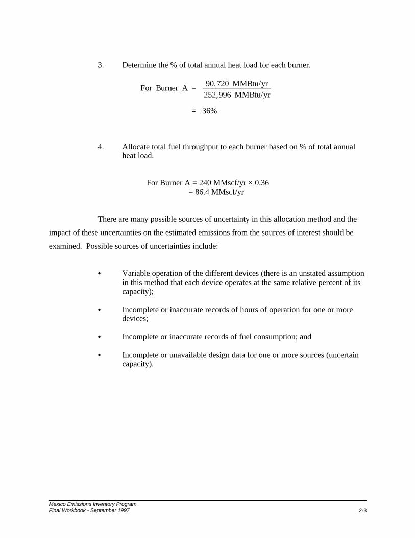
Mexico Emissions Inventory ProgramFinal Workbook - September 1997 2-3
For Burner A = 90,720 MMBtu/yr252,996 MMBtu/yr
= 36%
3. Determine the % of total annual heat load for each burner.
4. Allocate total fuel throughput to each burner based on % of total annualheat load.
For Burner A = 240 MMscf/yr × 0.36 = 86.4 MMscf/yr
There are many possible sources of uncertainty in this allocation method and the
impact of these uncertainties on the estimated emissions from the sources of interest should be
examined. Possible sources of uncertainties include:
C Variable operation of the different devices (there is an unstated assumptionin this method that each device operates at the same relative percent of itscapacity);
C Incomplete or inaccurate records of hours of operation for one or moredevices;
C Incomplete or inaccurate records of fuel consumption; and
C Incomplete or unavailable design data for one or more sources (uncertaincapacity).

Mexico Emissions Inventory ProgramFinal Workbook - September 19972-4
Example 2b
External Combustion Devices - Emission Factors
Introduction
This problem demonstrates the use of published emission factors to estimate
emissions. Although this problem may seem overly simplistic, it is a valuable estimation technique
that is used in virtually all emissions inventories.
Problem Statement
Estimate total NOx emissions from the four tortilla manufacturing machine burners
described in Example 2a.
Available Information
External combustion emission factors in AP-42 are classified based upon the heat
input of the external combustion device. This classification is shown below:
C Utility/large industrial (>100 MMBtu/hr);
C Small industrial (10-100 MMBtu/hr);
C Commercial (0.3-10 MMBtu/hr); and
C Residential (<0.3 MMBtu/hr).
Based upon this classification, burners A and C from Example 2a are small industrial devices
while burners B and D are commercial devices. None of the four burners have any emission
control devices attached to them.

Mexico Emissions Inventory ProgramFinal Workbook - September 1997 2-5
ETotal ' jn
d'1(FCd × EFd)
ETotal ' (2.45 × 2,240) % (0.95 × 1,600) % (1.63 × 2,240) % (1.77 × 1,600)' 5,488 % 1,520 % 3,651 % 2,832 ' 13,491 kg/yr ' 13.5 Mg/yr
Solution
From Table 1.4-2 of AP-42, the NOx emission factor for small industrial devices is
2240 kg/106 m3, while the emission factor for commercial devices is 1600 kg/106 m3. Emissions
from the burners in the tortilla factory are then calculated using the following equation:
where: ETotal = Total emissions (kg/yr);n = Number of devices;FCd = Fuel consumption for device d (106 m3/yr); andEFd = Emission factor for device d (kg/106 m3).
so

Mexico Emissions Inventory ProgramFinal Workbook - September 19972-6
Example 2c
External Combustion Devices - Other Estimating Techniques
Introduction
This problem demonstrates limitations of emission factors, which are widely used
in the development of emission inventories.
Emission factors are a widely used emission estimating technique primarily because
they are relatively inexpensive and easy to use. However, under certain circumstances, they may
not provide an accurate estimate of the emissions from a specific process. It is important to
understand that emission factors are based on available source test data. While the published
factors may be quite accurate for the specific equipment and conditions that were tested, they may
be significantly less accurate for other equipment and conditions.
When conducting an emissions inventory, it is not uncommon to encounter a
source for which there are no specific emission factors in the literature. In these cases, it has been
a common practice to use published emission factors for source types that appear to be similar.
While this practice of extrapolation may appear to be reasonable, it can cause significant errors in
the emission estimates.
This problem specifically focuses on the external combustion emission factors that
are found in Chapter 1 of AP-42 and presents an example to illustrate a case where these emission
factors were not applicable. Example source test data and associated calculations are also
presented.
Problem Statement
Estimate TOG emissions from a fume incinerator (an air pollution control device
designed to destroy the organic compounds emitted from sources such as large paint booths in the
automotive industry).

Mexico Emissions Inventory ProgramFinal Workbook - September 1997 2-7
Available Information
The inputs to the incinerator are the large exhaust air stream from the paint booth
(containing small quantities of organics to be destroyed) and natural gas as fuel to the incinerator
burners. The engineers who made emissions estimates for several fume incinerators were faced
with the problem of not having equipment-specific emission factors or source test data for the
incinerators. They examined the incinerator process and determined that the emissions would
result primarily from the fuel combustion because the quantity of pollutants in the paint booth
exhaust air was small in comparison to the fuel quantity. Knowing that emissions from boilers
also result only from the fuel combustion, the engineers logically decided to use the emission
factors in AP-42 for boilers with similar heat capacities to estimate the emissions for the fume
incinerator.
Unfortunately, this decision resulted in inaccurate emission estimates. In
subsequent source testing of the fume incinerators, it was shown that the actual NOx emissions
were approximately eight (8) times higher than the estimated emissions based on the boiler
emission factors. Upon detailed examination of the incinerator operation, it was determined that
the incinerator process parameters were substantially different than the boiler conditions in two
respects:
C The incinerators operated at much higher excess air concentrations than theboilers due to the quantity of exhaust air from the paint booths; and
C The incinerators operated at substantially higher temperatures than theboilers to ensure complete combustion of the organic pollutants.
Both of these conditions are conducive to the formation of thermal NOx (see
Note 1 at end of example), which explains the large difference between the estimated and actual
NOx emissions. These conditions also determine the extent of combustion, which affects the
formation of CO and the quantity of unburned organics (TOG) in the incinerator stack gas. Using
the published boiler emission factors in this case resulted in substantial errors in the estimated
emissions for the incinerators because the incinerators were operated at significantly different

Mexico Emissions Inventory ProgramFinal Workbook - September 19972-8
conditions than those encountered in the boiler source tests on which the emission factors were
based.
The correct methodology for estimating NOx emissions from the fume incinerator
was to conduct source testing. Costly new burner design trials and repeated source testing were
required to find a solution that reduced the NOx emissions from the fume incinerators to
acceptable levels without increasing TOG and CO emissions to unacceptable limits. Source test
data and calculated emission factors for NO2 (nitrogen dioxide), NOx, CO, and non-methane
hydrocarbon (NMHC) destruction removal efficiency (DRE) from one of the fume incinerators
are presented in Table 2-2. The following paragraphs present the methodology used for
calculation of the NOx and CO emission factors from the source test data. The NMHC DRE data
is presented for information only and to illustrate the relationship between NOx, CO, and TOG
emissions from external combustion for varying conditions.
Source test data are often obtained in units that are not useful for estimating
emissions. The test data may need to be converted to standard conditions (temperature and
pressure) for comparison with other data or may need to be converted from measured units to
reportable units. When source testing involves a series of process adjustments to determine the
influence of parameters such as temperature or percentage of excess air, then rapid on-site data
analysis may be required so the test team can judge the effect of each change. During the fume
incinerator source tests conducted in the example above, a spreadsheet was developed to allow
the rapid conversion of measured NOx emissions to the desired emission units. This spreadsheet
is presented as Table 2-2 in this workbook and the explanation of how the spreadsheet was used
to calculate NOx and CO emission factors is presented below.

Mexico Emissions Inventory ProgramFinal Workbook - September 1997 2-9

Mexico Emissions Inventory ProgramFinal Workbook - September 19972-10
Mexico Emissions Inventory ProgramFinal Workbook - September 1997 2-11
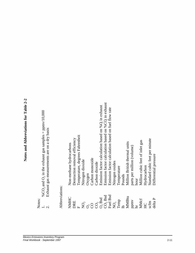
Not
es a
nd A
bbre
viat
ions
for
Tab
le 2
-2
Not
es:
1.%
CO
2 an
d O
2 in
the
exha
ust g
as s
ampl
es =
ppm
v/10
,000
2.E
xhau
st g
as m
easu
rem
ents
are
on
a dr
y ba
sis
Abb
revi
atio
ns:
NM
HC
Non
-met
hane
hyd
roca
rbon
sD
RE
Des
truc
tion
rem
oval
eff
icie
ncy
FT
empe
ratu
re, d
egre
es F
ahre
nhei
tN
O2
Nitr
ogen
dio
xide
O2
Oxy
gen
CO
Car
bon
mon
oxid
eC
O2
Car
bon
diox
ide
O2 B
sdE
mis
sion
fac
tor
calc
ulat
ion
base
d on
%O 2
in e
xhau
stC
O2 B
sdE
mis
sion
fac
tor
calc
ulat
ion
base
d on
%C
O 2 in
exh
aust
Fuel
Bsd
Em
issi
on f
acto
r ca
lcul
atio
n ba
sed
on f
uel f
low
rat
eN
Ox
Nitr
ogen
oxi
des
Tem
pT
empe
ratu
relb
Poun
dsM
MB
tuM
illio
n B
ritis
h th
erm
al u
nits
ppm
vpa
rts
per
mill
ion
(vol
ume)
hrho
urM
Mcf
Mill
ion
cubi
c fe
et o
f in
let g
asH
CH
ydro
carb
onsc
fmSt
anda
rd c
ubic
fee
t per
min
ute
delta
PD
iffe
rent
ial p
ress
ure

Mexico Emissions Inventory ProgramFinal Workbook - September 19972-12
E ' Cd × Fd × 20.920.9 & %O2
Given the following operating parameters, the NOx emission factor (lb/Btu) can be
estimated:
C Measured inlet and outlet source test data (all gas concentrations are on adry basis);
C Test temperature (EF);
C Exhaust gas flow rate (scfm); and
C Natural gas (fuel) firing rate.
The emission factor can be determined based on either the O2 or CO2
concentration in the exhaust gas or on the fuel firing rate. All three of these methods are
appropriate to use when calculating emission factors from source testing. Both the O2 and CO2
based emission factors are calculated using the F Factor method which was promulgated in the
October 6, 1975 United States Federal Register as a procedure to replace the original method of
determining emission factors. The U.S. EPA has published F factors for common fuels and the F
factor values used in these calculations were taken from Stack Sampling Technical Information
(U.S. EPA, 1978). The F factor for the O2 based emission factor for natural gas is 8,740
scf/MMBtu. The F factor for the CO2 based emission factor for natural gas is 1,040 scf/MMBtu.
In this example, the 3/25/92 test data at 1462 EF were used from Table 2-1.
The equation for calculating an O2 based NOx emission factor using the F factor method is:
where: E = Emission rate in lb/MMBtu;Cd = Pollutant concentration in dry exhaust gas minus pollutant
concentration in inlet gas (lb/scf);Fd = Oxygen based F factor (8,740 scf/MMBtu);%O2 = O2 percent in dry exhaust gas; and20.9 = Assumed O2 percent in inlet gas (ambient atmosphere).

Mexico Emissions Inventory ProgramFinal Workbook - September 1997 2-13
Cd '[C]ppmv × MW
CF1
Cd '
(129.4 & 0.25)scf NOx
106 scf exhaust gas ,
× 46 lblb&mole
380 scf/1 lb&mole
' 1.563 × 10&5lb NOx
scf exhaust gas
E ' 1.563 × 10&5lb NOx
scf× 8,740 scf
106 Btu× 20.9
20.9 & 17.25
E '0.78 lb NOx
106 Btu
The calculation of Cd in lb/scf exhaust gas from the measured concentrations of NOx (measured
as NO2) in ppmv is shown below.
where: [C]ppmv = Concentration of pollutant in exhaust minus concentration ofpollutant in inlet gas in ppmv (scf pollutant/MMscf exhaust gas);
MW = Molecular weight of NO2 (46 lb/lb-mole); andCF1 = Conversion factor based on ideal gas law that 1 lb-mole ideal gas =
380 scf.
Using data from Table 2-1 for the 3/25/92 test data at 1462 EF, the calculation of Cd is:
Then the calculation of the NOx emission factor using the oxygen based F factor is:

Mexico Emissions Inventory ProgramFinal Workbook - September 19972-14
E ' Cd × Fc × 100%CO2
%CO2 ' %CO2 (in dry exhaust gas as measured) &ppmv CO2 in inlet gas
10,000
E ' 2.11 &1,03010,000
' 2.007
E '1.563 × 10&5 lb NOx
scf× 1,040 scf
106 Btu× 100
2.007
E '0.81 lb NOx
106 Btu
The equation for calculating a CO2 based NOx emission factor using the F factor method is:
where: E = Emission rate (lb/MMBtu);Cd = Pollutant concentration in dry exhaust gas minus pollutant
concentration in inlet gas (lb/scf);Fc = Carbon dioxide based F factor (1,040 scf/MMBtu); and%CO2 = CO2 percent in dry exhaust gas minus CO2 percent in inlet gas.
The calculation of Cd in lb/scf from the measured concentrations of NOx in ppmv was done
above. The calculation of %CO2 is as follows:
Then the calculation of the NOx emission factor using the CO2 based F factor is:

Mexico Emissions Inventory ProgramFinal Workbook - September 1997 2-15
E 'Cd × Q × 60
FR
E '
1.563 × 10&5 lb NOx
scf× 3,454 scf
min× 60 min
hr ,
3.87 × 10⁶ Btu/hr
E '0.84 lb NOx
106 Btu
If the fuel firing rate is used to calculate a NOx emission factor, then the following equation is
used:
where: E = Emission rate (lb/MMBtu);Cd = Pollutant concentration in dry exhaust gas minus pollutant
concentration in inlet gas (lb/scf);Q = Exhaust flow rate (scf/minute);60 = Conversion factor from minutes to hours; andFR = Fuel firing rate (MMBtu/hour).
The calculation of Cd in lb/scf from the measured concentrations of NOx in ppmv was done
above.
So the emission factor based on the fuel firing rate is:
A comparison of the calculated emission factors with a emission factor from AP-42 is given in
Table 2-3.

Mexico Emissions Inventory ProgramFinal Workbook - September 19972-16
EFex ' EF ×(20.9 & O2(ex))
(20.9 & O2)
Table 2-3
Comparison of Calculated Emission Factors
Calculation Method Emission Factor (lb NOx/106 Btu)
O2 Based F Factor 0.78
CO2 Based F Factor 0.81
Fuel Firing Rate 0.84
AP-42, Table 1.4-2Uncontrolled Commercial Boiler*
0.10
* Assumes a natural gas fired higher heating value of 1,000 Btu/scf.
As mentioned earlier, the emission factor taken from AP-42 can be seen to be low by a factor of
eight (8).
In order to compare emission factors on an equivalent basis, it is sometimes necessary to adjust
the estimated emission factors to a given excess O2 concentration. This is often done for
regulatory purposes. This is done with the following equation.
where: EFex = NOx emission factor at desired excess O2 level (lb/MMBtu);EF = Calculated NOx emission factor (lb/MMBtu);20.9 = Assumed atmospheric O2 concentration (%);O2(ex) = Desired excess O2 concentration (%); andO2 = Measured O2 concentration in dry exhaust gas (%).
Using the O2-based emission factor calculated above, the NOx emission factor at 3% excess O2 for
the 3/25/92 test data at 1462 EF is calculated as:

Mexico Emissions Inventory ProgramFinal Workbook - September 1997 2-17
NOx (3%) ' 0.78lb NOx
106 Btu× 20.9 & 3
20.9 & 17.25
'3.83 lb NOx
106 Btu
The adjusted emission factor differs from the calculated emission factor because the desired
excess O2 concentration (3%) is quite different compared to the actual measured O2 concentration
(17.25%). If the desired excess O2 concentration is equal to the measured O2 concentration, then
the adjusted emission factor will be identical to the calculated emission factor.
Note 1: NOx is formed in external combustion in primarily two ways: thermal NOx and fuel NOx. ThermalNOx is formed when nitrogen and oxygen in the combustion air react at high temperatures in theflame. Fuel NOx is formed by the reaction of any nitrogen in the fuel with combustion air. ThermalNOx is the primary source of NOx in natural gas and light oil combustion and the most significantfactor affecting its formation is flame temperature. Excess air level and combustion air temperaturealso are factors in the formation of thermal NOx. Fuel NOx formation is dependent on the nitrogencontent of the fuel and can account for as much as 50% of the NOx emissions from the combustion ofhigh-nitrogen fuels - primarily heavy oils.

Mexico Emissions Inventory ProgramFinal Workbook - September 1997 3-1
Example 3
Residential Fuel Combustion
Introduction
This example illustrates a common situation where emissions must be estimated
with minimal data. In many instances, the inventory specialist will be faced with a shortage of
data that requires a creative approach to developing emission estimates. Because of the lack of
data, typical emission estimating methods are not always a feasible option. Rather, alternative
methods must be identified and examined. Each of the alternative methods will have positive and
negative points that must be evaluated before one is selected. In some cases, more than one of
the alternative methods may be selected in order to provide a possible range of emission estimates
(i.e., bounding calculations). Although one of the estimates will likely be incorporated into the
emissions database, the range of estimates provides one measure of the possible uncertainty
associated with that specific source category. This is an added benefit of performing bounding
calculations.
The following example is based upon the actual data and methodology used in an
air toxics inventory for Nogales, Sonora (Radian, 1997). This example is not intended to provide
a specific, recommended estimating method, rather, it is designed to present the thought processes
that should be employed in order to estimate emissions when faced with incomplete data.
Problem Statement
Determine the annual CO emissions from the combustion of non-commercial fuels.
Include only those fuels for heating or cooking purposes. Exclude any waste burning.

Mexico Emissions Inventory ProgramFinal Workbook - September 19973-2
Available Information
In Mexico, PEMEX (Petróleos Mexicanos), as well as some government agencies,
maintain fairly detailed statistics for the consumption of commercial fuels (e.g., distillate oil, LPG
[liquefied petroleum gas], etc.). However, significant quantities of non-commercial fuels are also
used in some areas of the country for residential heating and cooking. Examples of non-
commercial fuels include wood, other biomass, manure, scrap materials, tires, waste solvents, and
other waste-derived fuels. In this problem, these fuels are referred to as biomass/waste fuels.
Statistics for these types of fuels are almost nonexistent in most countries, including Mexico.
Although several local officials and residents cited statistics that 98% of the homes
in Nogales use LPG as of 1994 (Carrillo, 1996; Gastelum, 1996; Guerrero, 1996), the use of
waste derived fuels was considered a potentially significant source of emissions. Unfortunately,
very little data regarding the combustion of biomass/waste fuels were available for collection
during a local site visit. Overall population and household statistics were available for the
inventory domain, but residential biomass/waste fuel combustion rates were not.
Selection of Methodology
Ideally, biomass/waste fuel combustion rates derived from statistically valid
surveys would be combined with emission factors to yield emission estimates. However, because
survey data were not available, alternate estimation methods were used. Three possible methods
were devised that would allow biomass/waste combustion rates to be estimated. These included:
C The Heating Load method;
C The LPG Equivalence method; and
C The Micro-Inventory method.

Mexico Emissions Inventory ProgramFinal Workbook - September 1997 3-3
Each of these methods is described in detail below.
The Heating Load method:
This method uses the average monthly heating load for a typical Nogales house to
estimate emissions. The required average monthly heating load for a building can be determined
by the following equation (Harris et al., 1985):
Qi = (UA + 0.018V) × DDi × 24
where: Qi = Average monthly heating load (Btu/month) for month i;UA = Hourly transmission heat loss per degree of design temperature
difference (Btu/hr-EF);0.018V = Infiltration-ventilation hourly heat loss per degree of design
temperature difference (Btu/hr-EF);DDi = Monthly degree-days [65EF base temperature] (EF-day/month) for
month i; and24 = Conversion factor from days to hours.
The UA term is actually the product of an overall heat transmission coefficient for a given
structural element (U) and the surface area of that structural element (A). The V term represents
the hourly volume of infiltration air (the product of hourly air changes and space volume).
Guidelines for estimating values for UA and 0.018V for an entire building can be obtained from
various engineering handbooks (e.g., ASHRAE, 1997 - chapters 24 and 25). In order to estimate
these two variables, some characteristics of a “typical” house must be determined (building
material, average floor space, average building height, wall thickness, number of doors, number
and size of windows, etc.). A degree-day is the difference between a fixed base temperature
(usually 65EF) and the daily mean outdoor temperature, summed up for a specified period of time,
such as a month or a year. A higher degree-day total indicates a higher heating load. Degree-
days data are typically available from meteorological stations.
The required average annual heating load for a single household is calculated by
aggregating each of the average monthly heating loads using different degree days for each month
as shown below.
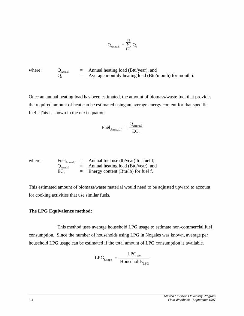
Mexico Emissions Inventory ProgramFinal Workbook - September 19973-4
QAnnual ' j12
i'1Qi
FuelAnnual,f 'QAnnual
ECf
LPGUsage 'LPGRes
HouseholdsLPG
where: QAnnual = Annual heating load (Btu/year); andQi = Average monthly heating load (Btu/month) for month i.
Once an annual heating load has been estimated, the amount of biomass/waste fuel that provides
the required amount of heat can be estimated using an average energy content for that specific
fuel. This is shown in the next equation.
where: FuelAnnual,f = Annual fuel use (lb/year) for fuel f;QAnnual = Annual heating load (Btu/year); andECf = Energy content (Btu/lb) for fuel f.
This estimated amount of biomass/waste material would need to be adjusted upward to account
for cooking activities that use similar fuels.
The LPG Equivalence method:
This method uses average household LPG usage to estimate non-commercial fuel
consumption. Since the number of households using LPG in Nogales was known, average per
household LPG usage can be estimated if the total amount of LPG consumption is available.
Mexico Emissions Inventory ProgramFinal Workbook - September 1997 3-5
Bio/WasteUsage ' LPGUsage ×ECLPG
ECBio/Waste
×EffLPG
EffBio/Waste
where: LPGUsage = Annual per household LPG usage (lb/yr);LPGRes = Annual total residential LPG usage (lb/yr); andHouseholdsLPG = Total households using LPG.
Using the energy content of LPG and typical biomass/waste fuels, equivalent average per
household biomass/waste usage can be estimated.
where: Bio/WasteUsage = Annual per household biomass/waste fuel usage (kg/yr);LPGUsage = Annual per household LPG usage (liters/yr);ECLPG = Energy content of LPG (kcal/liter);ECBio/Waste = Energy content of biomass/waste fuel (kcal/kg);EffLPG = Efficiency of LPG combustion; andEffBio/Waste = Efficiency of biomass/waste fuel combustion.
The Micro-Inventory method
This method involves performing a micro-inventory of 25 or 30 houses that use
biomass or waste fuels. A short interview should provide sufficient information. The most
important information is the quantity of fuel burned. Most people interviewed will not be able to
estimate annual or monthly usage, but they should be able to estimate usage over a shorter period
of time. Information should also be collected concerning seasonal usage variations and other
burning practices. Annual biomass or waste fuel usage could then be derived using these data.

Mexico Emissions Inventory ProgramFinal Workbook - September 19973-6
Analysis and Selection of Emission Estimating Methods
After establishing three alternative methods, it was necessary to select one of these
methods. The selection was based upon several selection criteria and general engineering
judgment. Selection criteria included such things as ease of use, representativeness, amount of
uncertainty, reasonableness, etc. For the Nogales, Sonora air toxics inventory, the LPG
Equivalence method was ultimately selected.
The Heating Load and Micro-Inventory methods were not selected for several
reasons:
C Potential for bias. It would be very difficult to assure that the “typicalhouse” selected for the Heating Load method actually represented thetypes of houses present in the inventory domain. Likewise, it would behard to guarantee that the households selected to be interviewed for theMicro-Inventory method would actually be representative of householdsthat burned biomass or waste fuels. The potential for bias would decreaseif large scale surveying was conducted to determine house characteristicsor fuel usage, but the associated cost would be prohibitive.
C Availability of data and types of assumptions. Although available dataare limited, the LPG Equivalence method uses these limited data andseveral reasonable assumptions to estimate emissions. The Heating Loadmethod, on the other hand, would require some additional data collection,as well as a few “less reasonable” assumptions.
C Reluctant survey participants. Given that LPG is used in 98% of thehomes, the number of households using biomass or waste fuels is in theminority. For the Micro-Inventory method, some of these householdsmight be reluctant to volunteer information regarding their burningpractices. Even if responses were given, there might be some questionabout the validity of the responses.
Mexico Emissions Inventory ProgramFinal Workbook - September 1997 3-7
HouseholdsBio/Waste ' %Bio/Waste × HouseholdsTotal ' 2% × 38,018 ' 760 households
Solution
Now that the LPG Equivalence method has been selected, it is possible to estimate
emissions. The four main steps are outlined below.
1. Determine number of households that use biomass/waste fuels forheating or cooking. Based upon census data, geographic informationsystem (GIS) data, and recent growth trends, it was estimated that thereare approximately 38,018 households in Nogales (Radian, 1997). Aspreviously mentioned, 98% of the Nogales households have been identifiedas using LPG. It was assumed that the remaining 2% of the Nogaleshouseholds use biomass/waste fuels. The total number of householdsusing biomass/waste is given below:
where: HouseholdsBio/Waste = Number of households using biomass/waste fuels;%Bio/Waste = Percentage of households using biomass/waste fuels; andHouseholdsTotal = Total number of households.
2. Determine per household LPG usage. Per household LPG usage isdetermined by dividing the total residential LPG usage by the number ofhouseholds that use LPG. PEMEX statistics indicated that the 1994 LPGusage for Nogales was 30,203,870 kilograms (Estrada, 1996). It has beendetermined that 80% of total LPG usage in Mexico is residential usage(Dirección General de Ecología et al., 1995).
The mass usage of LPG is converted to volume usage by estimating the density of
LPG. Unfortunately, the exact chemical composition and density of LPG in Nogales is unknown.
However, the approximate density of LPG in Nogales can be estimated using the dimensions of a
45 kilogram LPG cylinder and its reported weight. The measurements of a 45 kg LPG cylinder
indicated that the height is 1.04 m and the circumference is 1.19 m. As shown below, a cylinder
volume and then a density can be calculated from these cylinder dimensions. For a cylinder, the
volume is calculated as shown below:

Mexico Emissions Inventory ProgramFinal Workbook - September 19973-8
V ' Br 2h; C ' 2Br
V ' B C2B
2
h 'C 2h4B
V '(1.19 m)2 × 1.04 m
4 × 3.14' 0.1173 m 3
D 'mV
'45 kg
0.1173 m 3' 383.6 kg
m 3' 0.384 kg
liter
LPGv 'LPGm
D'
30,203,870 kg0.384 kg/liter
' 78,655,911 liters
where: V = cylinder volume (m);C = cylinder circumference (m);r = cylinder radius (m); andh = cylinder height (m).
The approximate density of the LPG is then:
where: D = LPG density (kg/liter);m = LPG mass in a cylinder (kg); andV = LPG cylinder volume (m3).
The conversion of LPG from kilograms to liters is then:
where: LPGv = Total LPG volume (liter);LPGm = Total LPG mass (kg); andD = LPG density (kg/liter).
Total residential LPG use is estimated to be 80% of the total LPG use with the remainder being
industrial/commercial usage (Dirección General de Ecología et al., 1995).

Mexico Emissions Inventory ProgramFinal Workbook - September 1997 3-9
LPGRes ' %Res × LPGTotal ' 80% × 78,655,911 liters ' 62,924,729 liters
HouseholdsLPG ' %LPG × HouseholdsTotal ' 98% × 38,018 ' 37,258
UsageLPG 'LPGRes
HouseholdsLPG
'62,924,729 liters
37,258 households' 1,689 liters/household
where: LPGRes = Residential LPG usage (liters/yr);%Res = Percentage of total LPG usage that is residential; andLPGTotal = Total LPG usage (liters/yr).
The number of households using LPG is given below:
where: HouseholdsLPG = Number of households using LPG;%LPG = Percentage of total households using LPG; andHouseholdsTotal = Number of total households.
Finally, per household LPG usage is calculated using the following equation:
where: UsageLPG = Annual per household LPG usage (liters/yr);LPGRes = Residential LPG usage (liters/yr); andHouseholdsLPG = Number households using LPG.
This per household LPG usage should be checked to see if it is reasonable. A very limited number
of informal interviews conducted with local residents indicate that a typical household uses one
large (45 kg) LPG cylinder per month during the summer and two large cylinders per month
during the winter (Monroy, 1996). Assuming that there are eight summer months and four winter
months, then a typical household would use approximately 16 large cylinders per year. Using the
LPG density calculated above and the weight per cylinder, the number of cylinders used per
household can be estimated.

Mexico Emissions Inventory ProgramFinal Workbook - September 19973-10
1,689 litershouseholds
× 0.384 kgliter
× 1 cylinder45 kg
'14.4 cylinders
household
LPG ' %prop × ECprop % %but × ECbut ' (0.6 × 6,090) % (0.4 × 6,790) ' 6,370 kcal/liter
Given that these estimates are within 10% of each other, the estimate of 1,689 liters of LPG per
household per year seems quite reasonable.
3. Convert per household LPG usage to per household biomass/wastefuel usage. The annual per household LPG usage value of 1,689liter/household calculated above represents the amount of LPG used by anaverage household for all of its heating and cooking requirements. Anequivalent amount of biomass/waste fuel can be estimated based upon fuelenergy contents.
Although local residents of Nogales refer to LPG as butane, the exact chemical
composition of Nogales LPG is unknown. The local LPG is assumed to be similar to the average
national composition of 60% propane and 40% butane (PEMEX, 1996). If the energy content of
propane is 6,090 kcal/liter and the energy content of butane is 6,790 kcal/liter (U.S. EPA, 1995a),
then the weighted energy content of LPG is calculated as shown below:
where: ECLPG = Energy content of LPG (kcal/liter);%prop = Percentage of propane in LPG;ECprop = Energy content of propane (kcal/liter);%but = Percentage of butane in LPG; andECbut = Energy content of butane (kcal/liter).
Assuming that the energy content of biomass/waste fuels is approximately that of pallet wood
(4,445 kcal/kg) (Summit et al, 1996) and that the combustion efficiencies of LPG and
biomass/waste fuels are equal, then the annual per household biomass/waste fuel usage can be
estimated.

Mexico Emissions Inventory ProgramFinal Workbook - September 1997 3-11
Bio/WasteUsage ' LPGUsage ×ECLPG
ECBio/Waste
×EffLPG
EffBio/Waste
Bio/WasteUsage '1,689 liters LPG
household× 6,370 kcal/liter LPG
4,445 kcal/kg bio/waste'
2,420 kg bio/wastehousehold
EmissionsCO ' Bio/WasteUsage × HouseholdsBio/Waste × EFCO
EmissionsCO '2,420 kg bio/waste
household× 760 households × 31 g CO
kg bio/waste
EmissionsCO ' 57,015 kg/yr CO ' 57.0 Mg/yr CO
where: Bio/WasteUsage = Annual per household biomass/waste fuel usage (kg/yr);LPGUsage = Annual per household LPG usage (liters/yr);ECLPG = Energy content of LPG (kcal/liter);ECBio/Waste = Energy content of biomass/waste fuels (kcal/kg);EffLPG = Efficiency of LPG combustion; andEffBio/Waste = Efficiency of biomass/waste fuel combustion.
4. Calculate overall CO emissions. Now that an annual per householdbiomass/waste fuel usage has been estimated, CO emissions can becalculated using the number of households and a CO emission factor. TheCO emission factor for biomass/waste fuels is based upon source test datafor combustion of Mexican pallet wood (Summit et al., 1996).
where: EmissionsCO = Total CO emissions (kg/yr or Mg/yr);Bio/WasteUsage = Annual per household biomass/waste fuel usage (kg/yr);HouseholdBio/Waste = Number of households using biomass/waste fuels; andEFCO = CO emission factor (g CO/kg bio/waste).
Discussion of Results
Although the annual CO emissions from residential biomass/waste combustion
were estimated to be 57 Mg/yr, the quality of this emission estimate and its underlying
Mexico Emissions Inventory ProgramFinal Workbook - September 19973-12
assumptions should be examined to determine areas of improvement and possible sources of
uncertainty. Several important issues are discussed below.
1. Number of households using biomass/waste fuels. Local officials hadestimated that 98% of the households used LPG. It was then assumed thatthe remaining 2% of the households used biomass/waste fuels. Thisassumption did not account for the possibility that some portion of theremaining 2% of households might use kerosene, distillate fuel, or othertypes of fuel.
2. Number of households using LPG. As mentioned earlier, local officialshad estimated that 98% of the households used LPG. However, it is notexactly clear what the basis of this estimate is or how accurate it is. Evenif the percentage of houses using LPG was slightly different, it could havea significant impact on the estimate of emissions from biomass/waste fuels. For example, if the actual percentage of households using LPG was 97%,instead of 98%, then emissions from LPG combustion would declineslightly. However, emissions from biomass/waste fuel combustion wouldbe greatly affected; the percentage of houses using biomass/waste wouldincrease from 2% to 3% -- a 50% increase.
3. Fraction of residential LPG use. It was assumed in this problem that80% of the overall LPG used is residential usage. This assumption isbased upon national statistics. Local consumption patterns may differ fromthis.
4. Combustion efficiencies. It was assumed in this problem that thecombustion efficiencies of LPG and biomass/waste fuels were equal. Inreality, the combustion of LPG is likely to be more efficient than thecombustion of biomass/waste fuels. This would increase biomass/ wasteemissions.
5. Fuel usage patterns. In converting LPG usage to biomass/waste fuelusage, an implicit assumption is that fuel usage patterns are the same. Thisis probably not the case. For example, if LPG is used for heating orcooking purposes, then the combustion device can easily be turned offwhen the desired amount of heat has been obtained. However,biomass/waste fuel combustion will often continue even after the desiredamount of heat has been reached, because it is not desirable or practical toextinguish the fire.
6. Composition of the biomass/waste fuel. It was assumed in this problemthat the biomass/waste fuel was pallet wood. In reality, biomass/waste fuelis likely to be composed of a wide variety of materials. Each of thesematerials will have its own energy content and emission factor.

Mexico Emissions Inventory ProgramFinal Workbook - September 1997 3-13
Given the limited data available for this emission estimation problem, it was necessary to make all
of the assumptions described above. Ideally, additional information could be gathered that would
eliminate the need for some of these assumptions. This would improve the quality of the emission
estimates and decrease the associated uncertainty.

Mexico Emissions Inventory ProgramFinal Workbook - September 1997 4-1
Example 4
Gasoline Distribution System
Introduction
The next example is divided into seven parts which are all related to the gasoline
distribution system. Although each part addresses an individual source category, these source
categories are often conceptually grouped together. This is primarily because the distribution of
gasoline is a potentially large source of evaporative total organic gas (TOG) emissions. A typical
gasoline distribution system may have hundreds or thousands of individual sources and it is
important that all of these sources are accounted for in an emissions inventory. By treating the
entire distribution system as a whole, it is often easier to ensure that all possible sources are
included.
A hypothetical gasoline distribution system with a manageable number of elements
is presented in Figure 4-1. This simplified system contains a bulk terminal and four gasoline
stations. Tank trucks transport the gasoline between the bulk terminal and the gasoline stations.
This system does not include the petroleum refinery upstream from the bulk terminal or transport
from the refinery to the bulk terminal by tank truck, rail car, or marine vessel. In reality, a
gasoline distribution system will usually be much more complex than the one presented here. The
distribution system in Figure 4-1 will be used throughout Example 4. The concepts presented in
these seven problems are not limited to gasoline distribution; they are also applicable to other
liquid fuels (e.g., aviation fuel, diesel, or LPG) and gaseous fuels (e.g., natural gas). The specific
details and emission factors, however, would be different.
Mexico Emissions Inventory ProgramFinal Workbook - September 19974-2

Mexico Emissions Inventory ProgramFinal Workbook - September 1997 4-3
Example 4a
Aboveground Bulk Storage Tank
Problem Statement
Estimate TOG emissions from standing and working losses at the bulk terminal’s
aboveground bulk storage tank.
Available Information
The total amount of RVP 9 gasoline pumped through the bulk terminal tank is
determined to be 10,000,000 liters per year (2,642,000 gallons per year). The bulk terminal tank
is a fixed roof aboveground storage tank (AST) with a capacity of 210,000 gallons. The AST has
a cone roof. The liquid height within the tank is unknown at any given time. Meteorological
conditions are assumed to be similar to Corpus Christi, Texas.
The following information is also known about the aboveground bulk storage tank:
Stored material = gasoline (RVP 9)Tank diameter (D) = 37.6 feetTank shell height (HS) = 24 feetTank average liquid height (HL) = 12 feet (the liquid height within the tank is unknown at any given time; assumed to be half of tank shell height)Tank capacity (VLX) = 210,000 gallonsTank color = light grayTank paint solar absorption (") = 0.54 (AP-42, Table 7.1-6 for light gray paint in good condition)Daily maximum ambient temperature (annual average) (TAX) = 81.6EF = 541.27ER (AP-42, Table 7.1-7)Daily minimum ambient temperature (annual average) (TAN) = 62.5EF = 522.17ER (AP-42, Table 7.1-7)Insolation (I) = 1521 Btu/ft2-day (AP-42, Table 7.1-7)Breather vent pressure setting (PBP) = 0.03 psig (AP-42 default value)Breather vent vacuum setting (PBV) = -0.03 psig (AP-42 default value)
Mexico Emissions Inventory ProgramFinal Workbook - September 19974-4
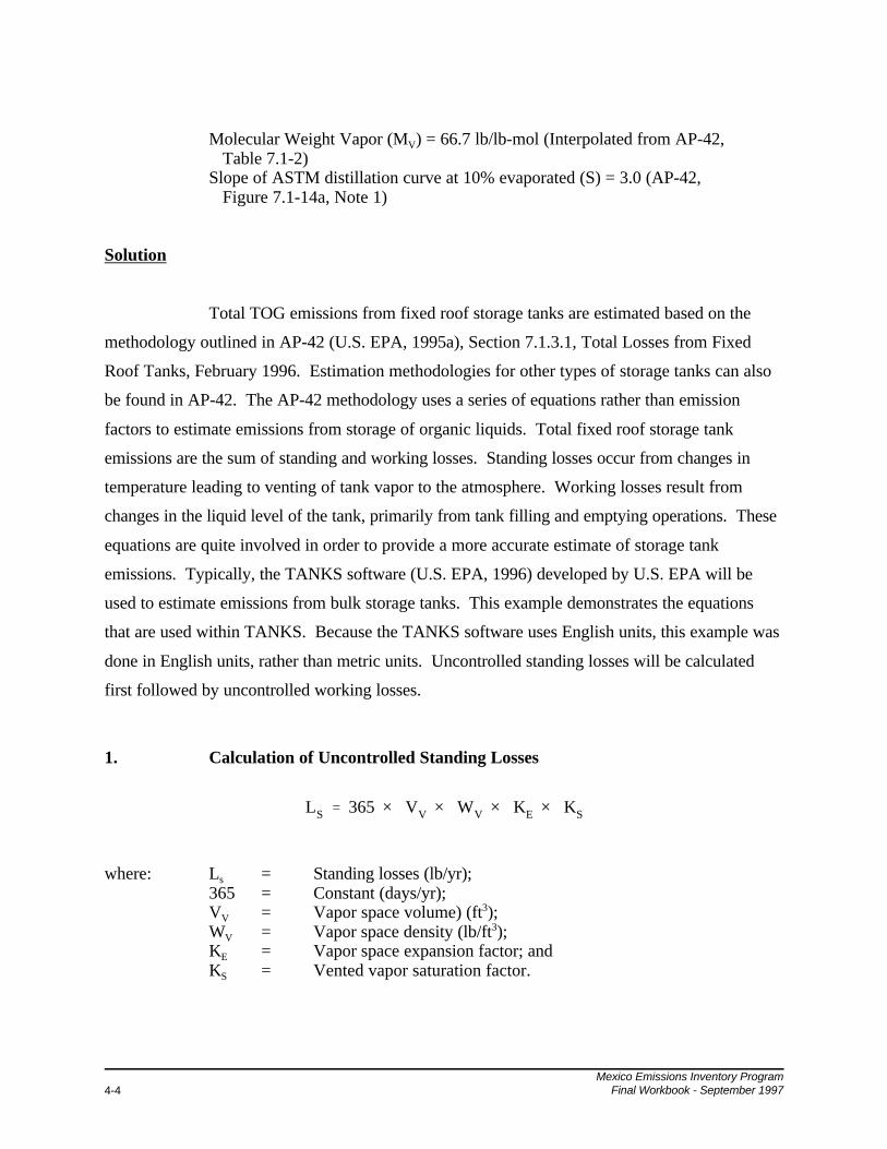
LS ' 365 × VV × WV × KE × KS
Molecular Weight Vapor (MV) = 66.7 lb/lb-mol (Interpolated from AP-42, Table 7.1-2)Slope of ASTM distillation curve at 10% evaporated (S) = 3.0 (AP-42, Figure 7.1-14a, Note 1)
Solution
Total TOG emissions from fixed roof storage tanks are estimated based on the
methodology outlined in AP-42 (U.S. EPA, 1995a), Section 7.1.3.1, Total Losses from Fixed
Roof Tanks, February 1996. Estimation methodologies for other types of storage tanks can also
be found in AP-42. The AP-42 methodology uses a series of equations rather than emission
factors to estimate emissions from storage of organic liquids. Total fixed roof storage tank
emissions are the sum of standing and working losses. Standing losses occur from changes in
temperature leading to venting of tank vapor to the atmosphere. Working losses result from
changes in the liquid level of the tank, primarily from tank filling and emptying operations. These
equations are quite involved in order to provide a more accurate estimate of storage tank
emissions. Typically, the TANKS software (U.S. EPA, 1996) developed by U.S. EPA will be
used to estimate emissions from bulk storage tanks. This example demonstrates the equations
that are used within TANKS. Because the TANKS software uses English units, this example was
done in English units, rather than metric units. Uncontrolled standing losses will be calculated
first followed by uncontrolled working losses.
1. Calculation of Uncontrolled Standing Losses
where: Ls = Standing losses (lb/yr);365 = Constant (days/yr);VV = Vapor space volume) (ft3);WV = Vapor space density (lb/ft3);KE = Vapor space expansion factor; andKS = Vented vapor saturation factor.

Mexico Emissions Inventory ProgramFinal Workbook - September 1997 4-5
VV 'B4
× D 2 × HVO
HVO ' HS & HL % HRO
HRO '13
× HR
HR ' RS × SR
Calculation of Vapor Space Volume (VV)
where: D = Tank diameter (ft); andHVO = Vapor space outage (ft).
where: HS = Tank shell height (ft);HL = Liquid height (ft), (if unknown this value can be assumed to be
0.5Hs [i.e., this means that the tank is, on average, one-half full]);and
HRO = Roof outage (ft).
where: HR = Tank roof height (ft).
where: RS = Tank shell radius (ft); andSR = Cone roof slope (ft/ft) (if unknown, use a standard value of 0.0625
ft/ft [AP-42, page 7.1-12])
For Bulk Terminal Tank:
RS = 0.5 × D= 0.5 × (37.6 ft) = 18.80 ft
SR = 0.0625 ft/ftHR = (18.80 ft) × (0.0625 ft/ft) = 1.175 ft
HRO = (1/3) × (1.175 ft) = 0.3917 ft

Mexico Emissions Inventory ProgramFinal Workbook - September 19974-6
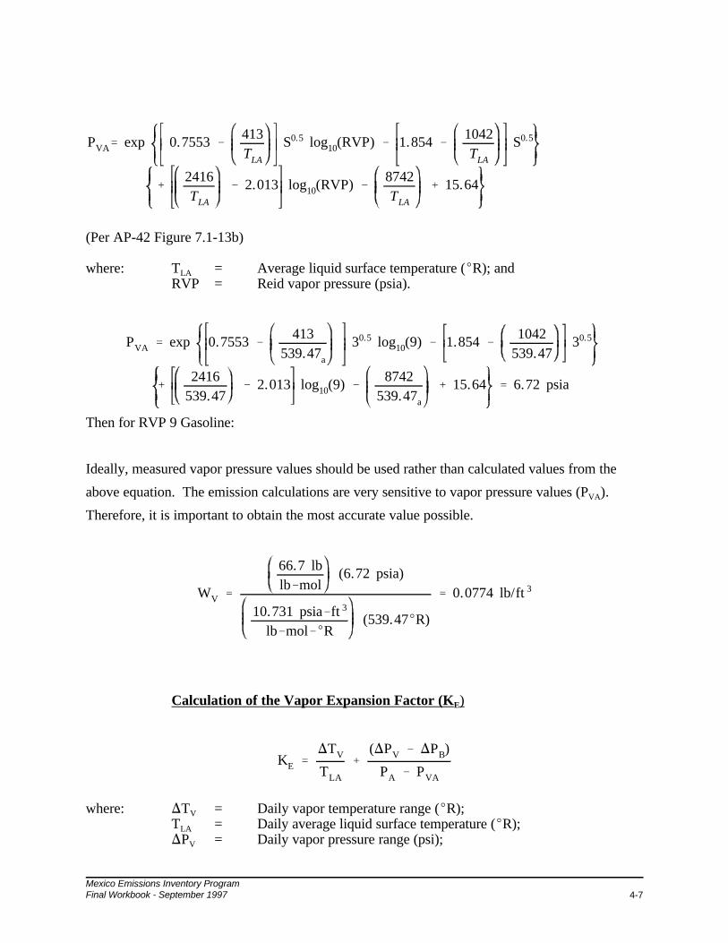
WV '(MV × PVA)
(R × TLA)
TLA ' 0.44TAA % 0.56TB % 0.0079"I
TAA '(TAX % TAN)
2
TB ' TAA % 6" & 1
HL = (0.5) × (24 ft) = 12 ft
HVO = 24 - 12 + 0.3917 = 12.39 ft
VV = (B/4) × (37.6 ft)2 × (12.39 ft) = 13,759 ft3
Calculation of Vapor Density (WV)
where: MV = Vapor molecular weight (lb/lb-mol);PVA = Vapor pressure at average liquid surface temperature (psia);R = Ideal gas constant (10.731 psia-ft3/lb-molER); andTLA = Daily average liquid surface temperature (ER).
where: TAA = Daily average ambient temperature (ER);TB = Liquid bulk temperature (ER); " = Tank paint solar absorption; andI = Daily total solar insolation factor (Btu/ft2-day) (The solar insolation
factor is a function of cloud cover and latitude. Some U.S. valuesare presented in AP-42, Table 7.1-7.)
where: TAX = Daily maximum ambient temperature (ER); and TAN = Daily minimum ambient temperature (ER).
TAA = (TAN + TAX)/2 = (522.17 + 541.27)/2 = 531.72ERTB = 531.72ER + 6(0.54) - 1 = 533.96ERTLA = (0.44) × (531.72ER) + (0.56) × (533.96ER) + (0.0079) × (0.54) ×
(1521 Btu/ft2-day) = 539.47ER
Mexico Emissions Inventory ProgramFinal Workbook - September 1997 4-7
PVA' exp 0.7553 &413TLA
S0.5 log10(RVP) & 1.854 &1042TLA
S0.5
%2416TLA
& 2.013 log10(RVP) &8742TLA
% 15.64
PVA ' exp 0.7553 &413
539.47a
30.5 log10(9) & 1.854 &1042
539.4730.5
%2416
539.47& 2.013 log10(9) &
8742539.47a
% 15.64 ' 6.72 psia
WV '
66.7 lblb&mol
(6.72 psia)
10.731 psia&ft 3
lb&mol&ER(539.47ER)
' 0.0774 lb/ft 3
KE ')TV
TLA
%()PV & )PB)
PA & PVA
(Per AP-42 Figure 7.1-13b) where: TLA = Average liquid surface temperature (ER); and
RVP = Reid vapor pressure (psia).
Then for RVP 9 Gasoline:
Ideally, measured vapor pressure values should be used rather than calculated values from the
above equation. The emission calculations are very sensitive to vapor pressure values (PVA).
Therefore, it is important to obtain the most accurate value possible.
Calculation of the Vapor Expansion Factor (KE)
where: )TV = Daily vapor temperature range (ER);TLA = Daily average liquid surface temperature (ER);)PV = Daily vapor pressure range (psi);

Mexico Emissions Inventory ProgramFinal Workbook - September 19974-8
PVX ' exp 0.7553 &413TLX
S 0.5 log10(RVP) & 1.854 &1042TLX
S 0.5
%2416TLX
& 2.013 log10(RVP) &8742TLX
% 15.64
PVN ' exp 0.7553 &413TLN
S 0.5 log10(RVP) & 1.854 &1042TLN
S 0.5
%2416TLN
& 2.013 log10(RVP) &8742TLN
% 15.64
)PB = Breather vent pressure setting range (psi);PA = Atmospheric pressure (normally 14.7 psia, however this may be
adjusted for high elevations if necessary); andPVA = Vapor pressure at the daily average surface temperature (psia).
)PB = PBP - PBV
where: PBP = Breather vent pressure settingPBV = Breather vent vacuum setting)PB = (0.03) - (-0.03) = 0.06 psia
)TV = 0.72)TA + 0.028"I
where: )TA = Daily average ambient temperature range (ER)
)TA = TAX - TAN
where: TAX = Daily maximum ambient temperature (ER); andTAN = Daily minimum ambient temperature (ER).)TA = 541.27 - 522.17 = 19.1ER
)TV = (0.72) × (19.1 ER) + (0.028) × (0.54) × (1521 Btu/ft2-day) = 36.75ER
TLA = 539.47ER (previously calculated))PV = PVX - PVN
(PVX and PVN estimated using same equation as PVA except using TLX and TLV
rather than TLA)
where: PVX = vapor pressure at the daily maximum liquid surface temp (psia); andPVN = vapor pressure at the daily minimum liquid surface temp (psia).
TLX = Maximum liquid surface temperature

Mexico Emissions Inventory ProgramFinal Workbook - September 1997 4-9
PVX ' exp 0.7553 &413
548.66a
30.5 log10(9) & 1.854 &1042
548.6630.5
%2416
548.66a
& 2.013 log10(9) &8742
548.66% 15.64 ' 7.93 psia
PVN ' exp 0.7553 &413
530.28a
30.5 log10(9) & 1.854 &1042
530.2830.5
%2416
530.28a
& 2.013 log10(9) &8742
530.28% 15.64 ' 5.67 psia
KE '36.75ER539.47ER
%(2.26 psia & 0.06 psia)(14.7 psia & 6.72 psia)
' 0.3438
= TLA + 0.25 ()TV) = 539.47 + 0.25 (36.75) = 548.66ERTLN = Minimum liquid surface temperature
= TLA - 0.25 ()TV) = 539.47 - 0.25 (36.75) = 530.28ER
Thus, for RVP 9 Gasoline:
)PV = PVX - PVN
= 7.93 - 5.67= 2.26 psia

Mexico Emissions Inventory ProgramFinal Workbook - September 19974-10
KS '1
1 % 0.053PVAHVO
Ks '1
1 % (0.053)(6.72)(12.39)' 0.1847
Calculation of Vapor Saturation Factor (KS)
where: PVA = Vapor pressure at daily average liquid surface temp (psia); andHVO = Vapor space outage (ft).
For RVP 9 Gasoline:
PVA = 6.72 psia; (previously calculated)HVO = 12.39 ft (previously calculated)
Solving for standing losses:
LS = 365 × VV × WV × KE × KS
VV = 13,759 ft3
WV = 0.0774 lb/ft3
KE = 0.3187KS = 0.1847LS = (365) × (13,759) × (0.0774) × (0.3438) × (0.1847)
= 24,683 lb/yr
2. Calculation of Uncontrolled Working Losses
LW = 0.0010 × MV × PVA × Q × KN × KP
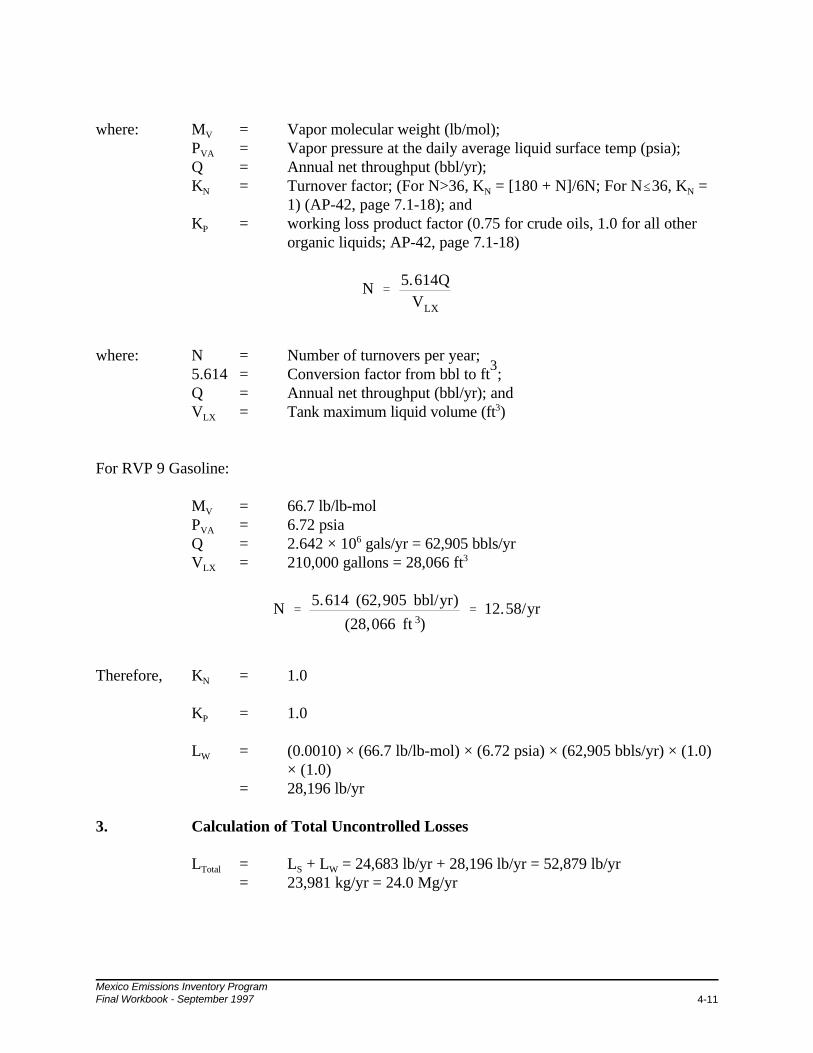
Mexico Emissions Inventory ProgramFinal Workbook - September 1997 4-11
N '5.614Q
VLX
N '5.614 (62,905 bbl/yr)
(28,066 ft 3)' 12.58/yr
where: MV = Vapor molecular weight (lb/mol);PVA = Vapor pressure at the daily average liquid surface temp (psia);Q = Annual net throughput (bbl/yr);KN = Turnover factor; (For N>36, KN = [180 + N]/6N; For N#36, KN =
1) (AP-42, page 7.1-18); andKP = working loss product factor (0.75 for crude oils, 1.0 for all other
organic liquids; AP-42, page 7.1-18)
where: N = Number of turnovers per year;5.614 = Conversion factor from bbl to ft
3;
Q = Annual net throughput (bbl/yr); andVLX = Tank maximum liquid volume (ft3)
For RVP 9 Gasoline:
MV = 66.7 lb/lb-molPVA = 6.72 psiaQ = 2.642 × 10⁶ gals/yr = 62,905 bbls/yrVLX = 210,000 gallons = 28,066 ft3
Therefore, KN = 1.0
KP = 1.0
LW = (0.0010) × (66.7 lb/lb-mol) × (6.72 psia) × (62,905 bbls/yr) × (1.0)× (1.0)
= 28,196 lb/yr
3. Calculation of Total Uncontrolled Losses
LTotal = LS + LW = 24,683 lb/yr + 28,196 lb/yr = 52,879 lb/yr= 23,981 kg/yr = 24.0 Mg/yr

Mexico Emissions Inventory ProgramFinal Workbook - September 19974-12
Example 4a - Supplemental Information
Estimating Individual Species
Introduction
In some air quality applications, estimates of individual species are required. For
some source categories, sampling for individual chemical species is performed. However, when
this sampling is impractical or too expensive, alternative methods must be used. For tank
emissions, Raoult’s Law provides a useful method for estimating emissions from individual
species.
Problem Statement
Using Raoult’s Law, estimate cyclohexane emissions from the bulk terminal tank
standing and working losses due to storage and pumping of RVP 9 gasoline.
Available Information
As estimated earlier, the bulk liquid temperature, (TLA), is 80 oF. The bulk terminal
tank is a fixed roof AST. After analysis of the RVP 9 gasoline, it is determined that the liquid
gasoline is 0.58 wt% cyclohexane (xliq,c = 0.0058).
Solution
To determine the speciated emissions from tank standing and working losses, the
following steps are necessary:
1. Determine the liquid phase speciation of gasoline in the tank.
2. Find the saturated vapor pressure of each species of concern at the bulkliquid temperature.

Mexico Emissions Inventory ProgramFinal Workbook - September 1997 4-13
3. Determine the true vapor pressure of the mixture at the bulk liquidtemperature.
4. Using Raoult’s Law, determine the vapor phase speciation of the gasolinein the tank.
5. Calculate the chemical-specific emissions using above steps and resultsfrom calculations such as those presented in Problem 4a.
Raoult’s Law can be used to determine the vapor phase mole fraction of a
particular constituent or species in a mixture based on the liquid phase mole fraction. It is
assumed that the vapor is an ideal gas and the liquid is an ideal solution. It also assumed that both
are well-mixed and in equilibrium with each other. Simply stated, if the liquid phase composition
in a tank is known, then the vapor phase composition in the tank’s vapor space can be calculated.
The assumptions of ideal behavior and vapor/liquid equilibrium are often not strictly enforced
since they are rarely achieved in the real world, and often Raoult’s law or another equation of
state is the only way to determine vapor phase compositions without actually sampling the tank to
measure them.
For a mixture of N species, Raoult’s law is expressed as:
YiP = XiPi sat; i = 1, 2, 3,...,N
where: Yi = Vapor phase mole fraction of component i;P = True vapor pressure of the mixture at the bulk liquid temperature;Xi = Liquid phase mole fraction of component i; andPi
sat = Saturated vapor pressure of species i at the bulk liquid temperature.
Also, xvap,c = the mass fraction of cyclohexane in the vapor phase
Note that extra steps may be required to convert mass fractions to mole fractions. The above
equation is written in terms of mole fractions, however data are commonly available as mass
fractions only.

Mexico Emissions Inventory ProgramFinal Workbook - September 19974-14
Yi 'XiP
Sati
P
Xc (mole fraction of cyclohexane in liquid phase) 'Xliq,cMWg
MWc
'(0.0058) (100)
84.16' 0.0069
Yc (mole fraction of cyclohexane in vapor phase) 'XcP
satc
Pg
'(0.0069) (2.069)
6.72' 0.00212
Xvap,c =YcMWc
MWv
'(0.00212) (84.16)
66.7
= 0.00267 lb cyclohexane / lb gasoline vapor
Given:Pg = True vapor pressure of gasoline = 6.72 psia at 80 oF
(previously calculated value for PVA; see Page 4-7)Pcyclohexane
sat = Saturated vapor pressure of cyclohexane = 2.069 psia (AP-42, Table 7.1-3)
Rearranging Raoult’s Law gives:
Before using this equation, the mass fraction in the liquid phase must be converted to a mole
fraction. This is done as follows, using the molecular weights:
MWg = Molecular weight of liquid gasoline = 100 lb/lb-mol (This istypically obtained from manufacturers or other published values.)
MWv = Molecular weight of gasoline vapor = 66.7 lb/lb-mol (extrapolatedfrom AP-42, Table 7.1-2)
MWc = Molecular weight of cyclohexane = 84.16 lb/lb-mol (AP-42, Table7.1-3)
We need the, xvap,c, the mass fraction of cyclohexane in the vapor phase. Hence, converting as
above:
Now, calculate cyclohexane emissions from standing and working losses from the aboveground
storage tanks.

Mexico Emissions Inventory ProgramFinal Workbook - September 1997 4-15
Lcyclohexane = 23,164 kg gasoline vaporyr
0.00267 kg cyclohexane1 kg gasoline vapor
= 62 kg cyclohexane/yr
LTotal = total standing and working losses
= 23,164 kg/yr

Mexico Emissions Inventory ProgramFinal Workbook - September 19974-16
Example 4a - Supplemental Information
Comparison of Raoult’s Law with Other Methods
Problem Statement
Compare results obtained using Raoult’s Law to measure vapor composition with
other techniques.
Solution
Table 4-1 (summer blend gasoline) presents an array of measured and predicted
results for the concentrations of several chemicals in vapor and liquid phase gasoline. The results
presented here are unrelated to the information presented in the previous Supplemental
Information section. As the data clearly show, Raoult’s Law predicts both more precise and
accurate vapor phase concentrations than either the Peng-Robinson or Redlich-Kwong-Soave
equations of state. Equations of state relate the intensive thermodynamic properties (e.g.,
temperature, pressure, or specific volume) of any substance. Information on the Peng-Robinson
or Redlich-Kwong-Soave equations of state can be found in standard chemical engineering
thermodynamics textbooks (i.e., Smith and Van Ness, 1987). In addition, Raoult’s Law is much
easier to use than either of the equations of state. The relative errors shown in the tables are also
within reason for the purposes of emissions estimation.
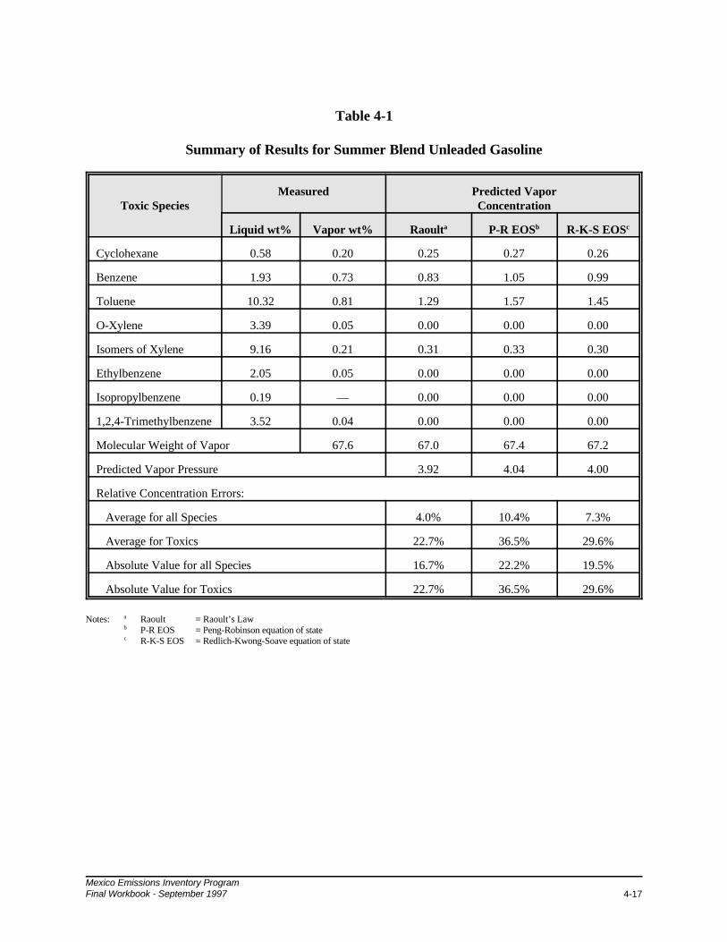
Mexico Emissions Inventory ProgramFinal Workbook - September 1997 4-17
Table 4-1
Summary of Results for Summer Blend Unleaded Gasoline
Toxic SpeciesMeasured Predicted Vapor
Concentration
Liquid wt% Vapor wt% Raoulta P-R EOSb R-K-S EOSc
Cyclohexane 0.58 0.20 0.25 0.27 0.26
Benzene 1.93 0.73 0.83 1.05 0.99
Toluene 10.32 0.81 1.29 1.57 1.45
O-Xylene 3.39 0.05 0.00 0.00 0.00
Isomers of Xylene 9.16 0.21 0.31 0.33 0.30
Ethylbenzene 2.05 0.05 0.00 0.00 0.00
Isopropylbenzene 0.19 — 0.00 0.00 0.00
1,2,4-Trimethylbenzene 3.52 0.04 0.00 0.00 0.00
Molecular Weight of Vapor 67.6 67.0 67.4 67.2
Predicted Vapor Pressure 3.92 4.04 4.00
Relative Concentration Errors:
Average for all Species 4.0% 10.4% 7.3%
Average for Toxics 22.7% 36.5% 29.6%
Absolute Value for all Species 16.7% 22.2% 19.5%
Absolute Value for Toxics 22.7% 36.5% 29.6%
Notes: a Raoult = Raoult’s Lawb P-R EOS = Peng-Robinson equation of statec R-K-S EOS = Redlich-Kwong-Soave equation of state

Mexico Emissions Inventory ProgramFinal Workbook - September 19974-18
Example 4b
Fugitive (Equipment Leak) Emissions
Problem Statement
Estimate fugitive TOG emissions from equipment leaks at the bulk terminal.
Example 4a addressed breathing and working losses associated with the aboveground storage
tank (AST) at the bulk terminal. This problem accounts for leaks of hydrocarbon vapors from
various types of process equipment.
Available Information
The hypothetical gasoline bulk terminal contains the following equipment types:
520 valves, 230 pump seals, 180 flanges, 120 connectors, and 70 other equipment types.
Equipment leak emission control techniques have not been implemented at the bulk terminal.
Solution
There are four approaches that are used to estimate fugitive TOG emissions.
These approaches, in order of increasing refinement, are:
C Average Emission Factor approach;
C Screening Ranges approach;
C EPA Correlation approach; and
C Unit-Specific Correlation approach.
These approaches are detailed in the U.S. EPA’s Protocol Document (U.S. EPA, 1995b). For a
facility with a relatively small number of equipment, such as a bulk terminal, usually only the first
two approaches would be used. For more complex facilities, such as refineries, the correlation

Mexico Emissions Inventory ProgramFinal Workbook - September 1997 4-19
Ee ' Ne × EFe × te
approaches are often utilized. Both the Average Emission Factor and Screening Ranges
approaches require equipment counts. However, the Screening Ranges approach requires some
additional information. Only the Average Emission Factor and Screening Ranges approaches will
be used in this problem.
Average Emission Factor Approach
Using the Average Emission Factor approach, total emissions for a specific
equipment type can be calculated using the following equation:
where: Ee = Uncontrolled fugitive emissions (kg/yr) for equipment type e;Ne = Number of equipment type e;EFe = Uncontrolled emission factor for equipment type e (kg/hr); andte = Annual time of process (hr/yr) (assumed to be 8,760 hours per
year).
The average emission factors presented in Table 4-2 for gasoline stored at bulk terminals are
taken from Table 2-3 of the Protocol Document. Other average emission factors also exist for
refineries, oil and gas production operations, and synthetic organic chemical manufacturing
operations. These other operations will have average emission factors for pressure relief valves,
open-ended lines, and sampling connections.
Table 4-2
Average Emission Factors
Equipment Type Emission Factor (kg/hr)Valves 0.000043
Pump Seals 0.00054
Fittings (Connectors and Flanges) 0.000008
Other Equipment 0.00013
The emissions for each equipment type are calculated below.

Mexico Emissions Inventory ProgramFinal Workbook - September 19974-20
EValves = 520 valves × 0.000043 kg/hr × 8,760 hr/yr ' 195.9 kg/yr
EPump Seals = 230 pump seals × 0.00054 kg/hr × 8,760 hr/yr ' 1,088 kg/yr
EFlanges = 180 flanges × 0.000008 kg/hr × 8,760 hr/yr ' 12.6 kg/yr
EConnectors = 120 connectors × 0.000008 kg/hr × 8,760 hr/yr ' 8.4 kg/yr
EOther = 70 other equipment × 0.00013 kg/hr × 8,760 hr/yr ' 79.7 kg/yr
ETotal ' 195.9 % 1,088 % 12.6 % 8.4 % 79.7 ' 1,385 kg/yr ' 1.4 Mg/yr of TOG
Ee ' ([NL × EFL] % [NNL × EFNL]) × te
The total fugitive emissions are then summed up as shown below.
Screening Ranges Approach
If the Screening Ranges approach is used, then each equipment component is
assigned either a “leak” or “no-leak” designation. This assignment is done by screening each
component. Screening is done by measuring the TOG concentration in the air right next to the
component. If the screening value is $10,000 ppmv, then the component is given a “leak”
designation. Conversely, if the screening value is <10,000 ppmv, then the component is given a
“no-leak” designation. Emissions from “leaking” components are estimated using “leaking”
emission factors; emissions from “non-leaking” components are estimated using “non-leaking”
emission factors. In spite of their designation, the “non-leaking” components are actually leaking
-- they just are leaking at a lesser rate than the “leaking” components.
Using the Screening Ranges approach, total emissions for a specific type of
equipment can be calculated using the following equation:
where: Ee = Uncontrolled fugitive emissions (kg/yr) for equipment type e;NL = Number of “leaking” equipment components;EFL = Uncontrolled emission factor for “leaking” equipment components
(kg/hr);NNL = Number of “non-leaking” equipment components;

Mexico Emissions Inventory ProgramFinal Workbook - September 1997 4-21
EValves = ([1 valve × 0.023 kg/hr] % [519 valves × 0.000015 kg/hr]) × 8,760 hr/yr ' 270 kg/yr
EPump Seals = ([0 pump seals × 0.077 kg/hr] % [230 pump seals × 0.00024 kg/hr]) × 8,760 hr/yr ' 484 kg/yr
EFlanges = ([2 flanges × 0.0065 kg/hr] % [178 flanges × 0.0000072 kg/hr]) × 8,760 hr/yr ' 125 kg/yr
EConnectors = ([2 connectors × 0.0065 kg/hr] % [118 connectors × 0.0000072 kg/hr]) × 8,760 hr/yr ' 121 kg/yr
EOther Equipment = ([1 other equipment × 0.034 kg/hr] % [69 other equipment × 0.000024 kg/hr] × 8,760 hr/yr ' 312 kg/yr
EFNL = Uncontrolled emission factor for “non-leaking” equipmentcomponents (kg/hr); and
te = Annual time of process (hr/yr) (assumed to be 8,760 hours peryear).
The screening ranges emission factors presented in Table 4-3 for gasoline stored at bulk terminals
are taken from Table 2-7 of the Protocol Document. Like the average emission factors presented
earlier, screening ranges emission factors also exist for refineries, oil and gas production
operations, and synthetic organic chemical manufacturing operations. There are also screening
ranges emission factors for pressure relief valves, open-ended lines, and sampling connections.
Table 4-3
Screening Range Emission Factors
Equipment Type“Leaking” Emission Factor
($$10,000 ppmv) (kg/hr)“Non-Leaking” Emission Factor
(<10,000 ppmv) (kg/hr)
Valves 0.023 0.000015
Pump Seals 0.077 0.00024
Fittings (Connectors andFlanges)
0.0065 0.0000072
Other Equipment 0.034 0.000024
After screening, it is determined that the following pieces of equipment are “leaking” (i.e.,
screening value $ 10,000 ppmv): 1 valve, 2 flanges, 2 connectors, and 1 piece of other equipment.
The TOG emissions for each equipment type are then calculated as follows.

Mexico Emissions Inventory ProgramFinal Workbook - September 19974-22
ETotal ' 270 % 484 % 125 % 121 % 312 ' 1,312 kg/yr ' 1.3 Mg/yr
The total fugitive emissions are then summed up as shown below.
Although this sample problem is hypothetical, it shows that a more refined approach might
produce significantly different results than a more simplified approach. In general, the Screening
Ranges approach will give lower results than the Average Emission Factor approach. However,
the increased data collection requirements associated with the more refined approaches must be
weighed against the need for more accurate results.
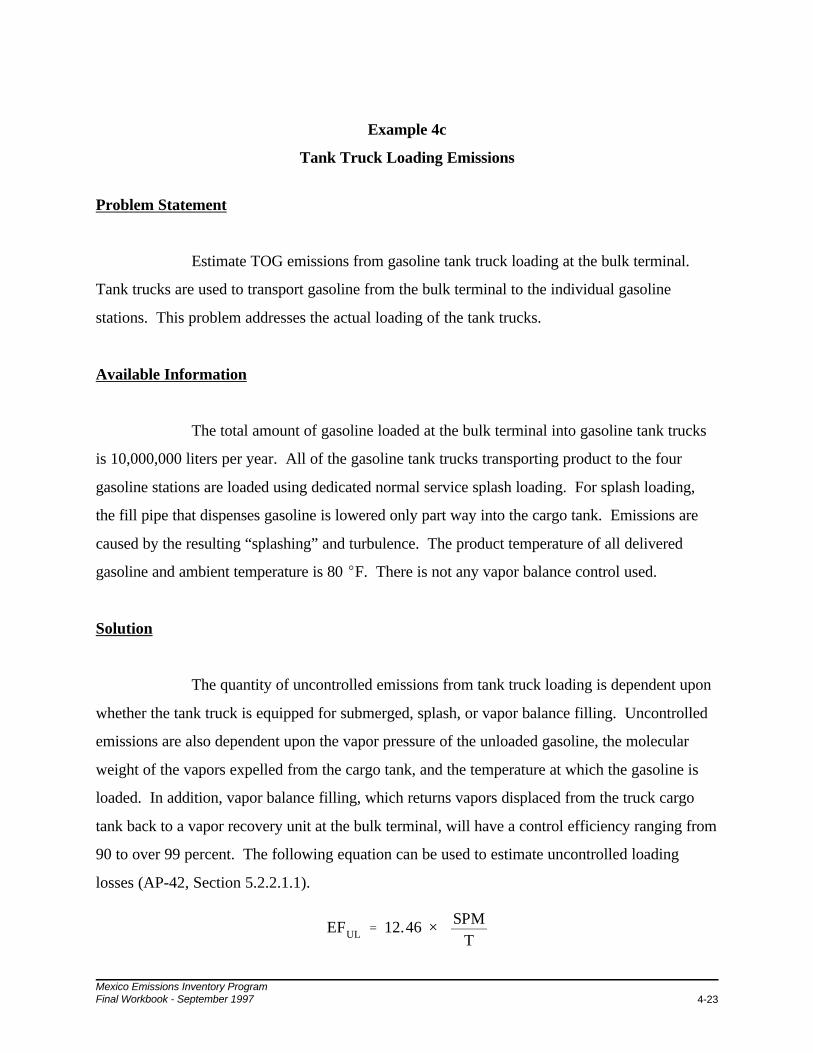
Mexico Emissions Inventory ProgramFinal Workbook - September 1997 4-23
EFUL ' 12.46 × SPMT
Example 4c
Tank Truck Loading Emissions
Problem Statement
Estimate TOG emissions from gasoline tank truck loading at the bulk terminal.
Tank trucks are used to transport gasoline from the bulk terminal to the individual gasoline
stations. This problem addresses the actual loading of the tank trucks.
Available Information
The total amount of gasoline loaded at the bulk terminal into gasoline tank trucks
is 10,000,000 liters per year. All of the gasoline tank trucks transporting product to the four
gasoline stations are loaded using dedicated normal service splash loading. For splash loading,
the fill pipe that dispenses gasoline is lowered only part way into the cargo tank. Emissions are
caused by the resulting “splashing” and turbulence. The product temperature of all delivered
gasoline and ambient temperature is 80 EF. There is not any vapor balance control used.
Solution
The quantity of uncontrolled emissions from tank truck loading is dependent upon
whether the tank truck is equipped for submerged, splash, or vapor balance filling. Uncontrolled
emissions are also dependent upon the vapor pressure of the unloaded gasoline, the molecular
weight of the vapors expelled from the cargo tank, and the temperature at which the gasoline is
loaded. In addition, vapor balance filling, which returns vapors displaced from the truck cargo
tank back to a vapor recovery unit at the bulk terminal, will have a control efficiency ranging from
90 to over 99 percent. The following equation can be used to estimate uncontrolled loading
losses (AP-42, Section 5.2.2.1.1).

Mexico Emissions Inventory ProgramFinal Workbook - September 19974-24
VMWi ' VMWx %RVPx & RVPi
RVPx & RVPn
VMWn&VMWx
where: EFUL = Uncontrolled loading loss emission factor (lb/1000 gal);S = Saturation factor;P = True vapor pressure of gasoline (pounds per square inch absolute
[psia]);M = Molecular weight of vapors (lb/lb-mole); andT = Temperature of loaded gasoline (ER).
Saturation factors (S) for various modes of operation, which represent how close the expelled
vapor comes to saturation, are presented in Table 4-4.
Table 4-4
Saturation Factors (S) for Calculating Petroleum Liquid Loading Losses
Type of Service Splash Loading Submerged LoadingClean Cargo Tank 1.45 0.50
Dedicated Normal Service 1.45 0.60Dedicated Vapor Balance Service
1.00 1.00
True vapor pressures and molecular weights of gasoline vapors can be derived from Figure 7.1-5,
Figure 7.1-6, and Table 7.1-2 of AP-42. Excerpted information from Table 7.1-2 is presented in
Table 4-5.
Table 4-5
Physical Properties of Gasoline
GasolineRVP
Vapor MolecularWeight at 60EEF (lb/lb-
mole)
True Vapor Pressure (psi)
40 EEF 50 EEF 60 EEF 70 EEF 80 EEF 90 EEF 100 EEF13 psia 62 4.7 5.7 6.9 8.3 9.9 11.7 13.810 psia 66 3.4 4.2 5.2 6.2 7.4 8.8 10.57 psia 68 2.3 2.9 3.5 4.3 5.2 6.2 7.4
The vapor molecular weight and true vapor pressure for RVP 9 gasoline values must be
interpolated from values presented in the table above. This interpolation is shown below.

Mexico Emissions Inventory ProgramFinal Workbook - September 1997 4-25
TVPi ' TVPx &RVPx & RVPi
RVPx & RVPn
TVPx&TVPn
VMW9 ' 66 %10&910&7
68&66 ' 66.7 lb/lb&mole
TVP9 ' 7.4 &10&910&7
7.4&5.2 ' 6.7 psi
EFUL(RVP9) '12.46 × 1.45 × 6.7 × 66.7
540' 14.95 lb/1000 gal
EFCL ' (1 & CE) × EFUL
where: VMWi = Vapor molecular weight interpolated to RVP 9;VMWx = Vapor molecular weight at maximum RVP (10) in
interpolation range;VMWn = Vapor molecular weight at minimum RVP (7) in
interpolation range;RVPi = Interpolated RVP (9);RVPx = Maximum RVP (10);RVPn = Minimum RVP (7);TVPi = True vapor pressure interpolated to RVP 9;TVPx = True vapor pressure at maximum RVP (10); andTVPu = True vapor pressure at minimum RVP (7).
The saturation factor for dedicated normal service splash loading is 1.45. Finally, converting the
gasoline temperature from Fahrenheit degrees to Rankine degrees gives a temperature of 540 ER.
Thus, the uncontrolled loading emission factors are calculated below.
Controlled loading emission factors are then calculated using the following equation.
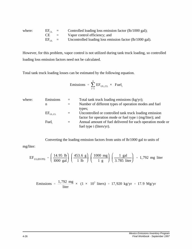
Mexico Emissions Inventory ProgramFinal Workbook - September 19974-26
Emissions ' jn
i'1EFUL,CL × Fueli
EFUL(RVP9) '14.95 lbl000 gal
453.6 g1 lb
1000 mg1 g
1 gal3.785 liter
' 1,792 mg liter
Emissions '1,792 mg
liter× (1 × 10⁷ liters) ' 17,920 kg/yr ' 17.9 Mg/yr
where: EFCL = Controlled loading loss emission factor (lb/1000 gal);CE = Vapor control efficiency; andEFUL = Uncontrolled loading loss emission factor (lb/1000 gal).
However, for this problem, vapor control is not utilized during tank truck loading, so controlled
loading loss emission factors need not be calculated.
Total tank truck loading losses can be estimated by the following equation.
where: Emissions = Total tank truck loading emissions (kg/yr);n = Number of different types of operation modes and fuel
types;EFUL,CL = Uncontrolled or controlled tank truck loading emission
factor for operation mode or fuel type i (mg/liter); andFueli = Annual amount of fuel delivered for each operation mode or
fuel type i (liters/yr).
Converting the loading emission factors from units of lb/1000 gal to units of
mg/liter:

Mexico Emissions Inventory ProgramFinal Workbook - September 1997 4-27
Example 4d
Tank Truck Transit Emissions
Problem Statement
After gasoline is loaded into tank trucks, it is transported to gasoline stations.
Although tank trucks do have enclosed cargo tanks, emissions do occur while in transit. This
problem focuses on the emissions that occur while the tank truck is in transit.
Estimate TOG emissions from gasoline tank trucks in transit from the bulk
terminal to PEMEX gasoline stations A, B, C, and D.
Available Information
The following amounts of gasoline are transported to the four gasoline stations for
sale:
Gasoline Station Gasoline Dispensed (liters/yr)
A 4,000,000
B 2,500,000
C 2,000,000
D 1,500,000
Solution
The quantity of emissions from gasoline tank trucks is dependent upon the extent
of venting that occurs during transit, which in turn depends upon the vapor tightness of the tank,
the pressure relief valve settings, the pressure in the tank at the start of the trip, the vapor pressure
of the fuel being transported, and the degree of fuel vapor saturation of the space in the tank. The
emissions are not directly proportional to the time spent in transit.

Mexico Emissions Inventory ProgramFinal Workbook - September 19974-28
Emissions ' jn
i'1([EFl,c % EFr,c] × Fueli)
AP-42, Table 5.2-5 presents transit loss emission factors for gasoline tank trucks
both loaded with product and returning with vapors for RVP 10 gasoline. These emission factors
are presented in Table 4-6 for both “typical” and “extreme” transit conditions. Extreme
conditions refer to the unlikely event that all of the determining factors listed above combine to
cause maximum emissions.
Table 4-6
Total Uncontrolled Emission Factors for Gasoline Tank Trucks
Transit ConditionsLoaded with product (mg/liter
of gasoline)Returning with vapor(mg/liter of gasoline)
Typical 0 - 1.0 0 - 13.0
Extreme 0 - 9.0 0 - 44.0
Total transit loss emissions will include both the trip from the bulk terminal to the
gas stations (loaded with product) and the return trip from the gas stations back to the bulk
terminal (empty tanks). Total transit loss emissions can be estimated by the following equation.
where: Emissions = Total refueling emissions (kg/yr);n = Number of gasoline stations;EFl,c = “Loaded with product” transit loss emission factor for
gasoline transported to station i under transit conditions c(mg/liter);
EFr,c = “Returning with vapor” transit loss emission factor forgasoline transported to station i under transit conditions c(mg/liter); and
Fueli = Annual amount of fuel dispensed from gasoline station i(liters/yr).
Assuming that gasoline transported to stations A, B, and C is transported under
“typical” conditions and gasoline transported to stations D is transported under “extreme”

Mexico Emissions Inventory ProgramFinal Workbook - September 1997 4-29
Emissions ' ([0.5 % 6.5] mg/liter) × ([4 × 10⁶] % [2.5 × 10⁶] % [2 × 10⁶] liters)
% ([4.5 % 22] mg/liter) × (1.5 × 10⁶ liters)
' 59.5 kg/yr % 39.75 kg/yr
' 99 kg/yr
conditions, estimate overall transit emissions. For each emission factor, assume that the midpoint
of the range listed in the table above provides a reasonable estimate.
Note that the amount of gasoline sold in this problem is equal to the amount of
gasoline transported. This, however, is not always the case. If transit emissions are estimated for
the transport of gasoline from a refinery to a bulk terminal and then from the bulk terminal to
gasoline stations, then the transit emissions would be twice as much because the gasoline is
“transported” twice. Gasoline may also be transported through an inventory domain even though
its origin and/or destination may lie outside of the inventory domain.

Mexico Emissions Inventory ProgramFinal Workbook - September 19974-30
Example 4e
Underground Tank Filling Emissions
Problem Statement
Estimate TOG emissions from gasoline tank truck unloading at gasoline stations A,
B, C, and D. After tank trucks arrive at the gasoline stations, they unload their cargo into the
underground storage tanks at the gasoline station. This unloading is similar to the loading of the
tank trucks at the bulk terminal.
Available Information
The following amounts of gasoline are transported to the four gasoline stations for
sale:
Gasoline Station Gasoline Delivered (liters/yr)
A 4,000,000
B 2,500,000
C 2,000,000
D 1,500,000
The following modes of operation are in place at the four gasoline stations:
Gasoline Station Mode of Operation
A Submerged loading - normal service
B Submerged loading - vapor balance service
C Splash loading - normal service
D Splash loading - normal service

Mexico Emissions Inventory ProgramFinal Workbook - September 1997 4-31
Emissions ' jn
i'1EFi × Fueli
For splash loading, the fill pipe that dispenses gasoline is lowered only part way
into the storage tank. Emissions are caused by the resulting “splashing” and turbulence. For
submerged loading, the fill pipe extends nearly to the bottom of the storage tank. Because of this,
liquid turbulence and the resulting emissions are reduced relative to splash loading. Vapor
balance service retrieves the vapors displaced during gasoline unloading and transports the vapors
back to the tank truck.
Solution
The quantity of emissions from underground tank filling is dependent upon
whether the gasoline station tank is equipped for submerged, splash, or submerged vapor balance
filling. Vapor balance filling, which returns vapors displaced from the gasoline station tank back
to the tank truck, will have a control efficiency ranging from 93 to 100 percent relative to
uncontrolled emissions. Table 4-7 shows the emission factors for underground tank filling (AP-
42, Table 5.2-7).
Table 4-7
Emission Factors for Underground Tank Filling at Gasoline Stations
Type of Operation Emission Factor (mg/liter throughput)
Submerged 880
Splash 1,380
Balanced Submerged 40
Total underground tank filling emissions can be estimated by the following equation.

Mexico Emissions Inventory ProgramFinal Workbook - September 19974-32
where: Emissions = Total underground tank filling emissions (kg/yr);EFi = Underground tank filling emission factor for operation type i
(mg/liter); andFueli = Annual amount of fuel delivered for operation type i
(liters/yr).
Emissions = (880 [4 × 10⁶] + 40 [2.5 × 10
6] + 1,380 [2 × 10
6] + 1,380 [1.5 × 10
6])
Emissions = 3,520 + 100 + 2,760 + 2,070 = 8,450 kg/yr= 8.45 Mg/yr

Mexico Emissions Inventory ProgramFinal Workbook - September 1997 4-33
Example 4f
Underground Tank Breathing Emissions
Problem Statement
Estimate TOG emissions from underground tank breathing at gasoline stations A,
B, C, and D.
Available Information
The following amounts of gasoline were sold at the four gasoline stations in the
region:
Gasoline Station Gasoline Dispensed (liters/yr)
A 4,000,000
B 2,500,000
C 2,000,000
D 1,500,000
Total 10,000,000
Solution
The quantity of emissions from underground breathing losses is mainly dependent
upon evaporation and barometric pressure changes. Also, the frequency of gasoline withdrawal
from the tank also has an effect on the emissions quantity because fresh air brought into the tank
will enhance the evaporation rate. An average breathing emission rate for U.S. gasoline stations
has been estimated to be 120 mg/liter of gasoline throughput (AP-42, Table 5.2-7). The tank
equations presented in AP-42, Section 7 could be used to estimate emissions from underground
gasoline storage tanks at gasoline stations. However, the large number of gasoline station tanks

Mexico Emissions Inventory ProgramFinal Workbook - September 19974-34
Emissions ' jn
i'1EFUB × Fueli
Emissions = (120[4 × 10⁶] % 120[2.5 × 10⁶] % 120[2 × 10⁶] % 120[1.5 × 10⁶])
Emissions = 480 % 300 % 240 % 180 ' 1,200 kg/yr ' 1.2 Mg/yr
usually precludes the use of these equations. Total underground breathing losses can be estimated
using the following equation with the average breathing emission rate.
where: Emissions = Total underground tank breathing emissions (kg/yr);n = Number of gasoline stations;EFUB = Underground breathing loss emission factor for gasoline
station i (mg/liter) [U.S. average value - 120 mg/liter];Fueli = Annual amount of fuel delivered to gasoline station i
(liters/yr).

Mexico Emissions Inventory ProgramFinal Workbook - September 1997 4-35
Example 4g
Vehicle Refueling Emissions
Problem Statement
Estimate TOG emissions from vehicle refueling at gasoline stations A, B, C, and
D. Refueling emissions consist of both vapors displaced from the vehicle tank by dispensed
gasoline, as well as gasoline spillage.
Available Information
The four gasoline stations in the distribution system dispense the following
quantities of RVP 9 of gasoline:
Gasoline Station Gasoline Dispensed (liters/yr)
A 4,000,000
B 2,500,000
C 2,000,000
D 1,500,000
The temperature of the dispensed fuel is 24 EC (75 EF) and the temperature of the
fuel in the vehicle tank is about 30 EC (86 EF). Stations A and C are uncontrolled; stations B and
D are controlled using vapor control which transfers displaced vapors from the vehicle fuel tank
back to the underground storage tank vapor space.
Solution
The quantity of emissions from displaced vapors depends upon the gasoline
temperature, vehicle tank temperature, gasoline Reid vapor pressure (RVP), and dispensing rate.

Mexico Emissions Inventory ProgramFinal Workbook - September 19974-36
EFu ' 264.2[(&5.909) & 0.0949()T) % 0.0884(TD) % 0.485(RVP)]
EFu ' 264.2[(&5.909) & 0.0949(11E) % 0.0884(75E) % 0.485(9)] ' 1,068 mg/liter
EFc ' (1 & CE) × EFu
The following equation can be used to estimate uncontrolled displacement losses based upon the
factors mentioned above (AP-42, Section 5.2.2.3).
where: EFu = Uncontrolled TOG emission factor for vehicle refueling(mg/liter);
)T = Difference between temperature of fuel in vehicle tank andtemperature of dispensed fuel (EF);
TD = Temperature of dispensed fuel (EF); andRVP = Reid vapor pressure (psia).
The uncontrolled displacement loss emission factors for each gas station are
calculated below.
Controlled displacement losses must be estimated for stations B and D. AP-42
indicates that typical U.S. vapor control efficiencies range from 88-92% (AP-42, Section 5.2.2.3).
The equation for calculating a controlled displacement loss factor is shown below.
where: EFc = Controlled TOG emission factor for vehicle refueling(mg/liter);
CE = Vapor control efficiency; andEFu = Uncontrolled TOG emission factor for vehicle refueling
(mg/liter).
Assuming that the Stage II vapor control efficiency is 88%, then the controlled
displacement loss emission factors for stations B and D are calculated as follows.

Mexico Emissions Inventory ProgramFinal Workbook - September 1997 4-37
EFcB, cD ' (1 & 0.88) × 1,068 mg/liter ' 128 mg/liter
Emissions ' jn
i'1([EFu,c % EFs] × Fueli)
Emissions ' ([1,068 % 80][4 × 10⁶] % [128 % 80][2.5 × 10⁶] % [1,068 % 80][2 × 10⁶]% [128 % 80][1.5 × 10⁶])
In addition to displacement losses, spillage losses occur during vehicle refueling.
The U.S. spillage emission factor (EFs) has been estimated to be 80 mg/liter of fuel dispensed.
The actual amount of spillage is dependent upon several factors such as gasoline station business
characteristics, tank configuration, and operator techniques.
Total refueling losses can be estimated by the following equation.
where: Emissions = Total refueling emissions (kg/yr);n = Number of gasoline stations;EFu,c = Uncontrolled or controlled displacement loss
emission factor for gasoline station i (mg/liter);EFs = Spillage emission factor for gasoline station i
(mg/liter); andFueli = Annual amount of fuel dispensed from gasoline
station i (liters/yr).
Assuming that the U.S. spillage emission factor of 80 mg/liter is appropriate for
Mexico, estimate overall refueling emissions.
Emissions = 4,592 + 520 + 2,296 + 312 = 7,720 kg/yr = 7.72 Mg/yr
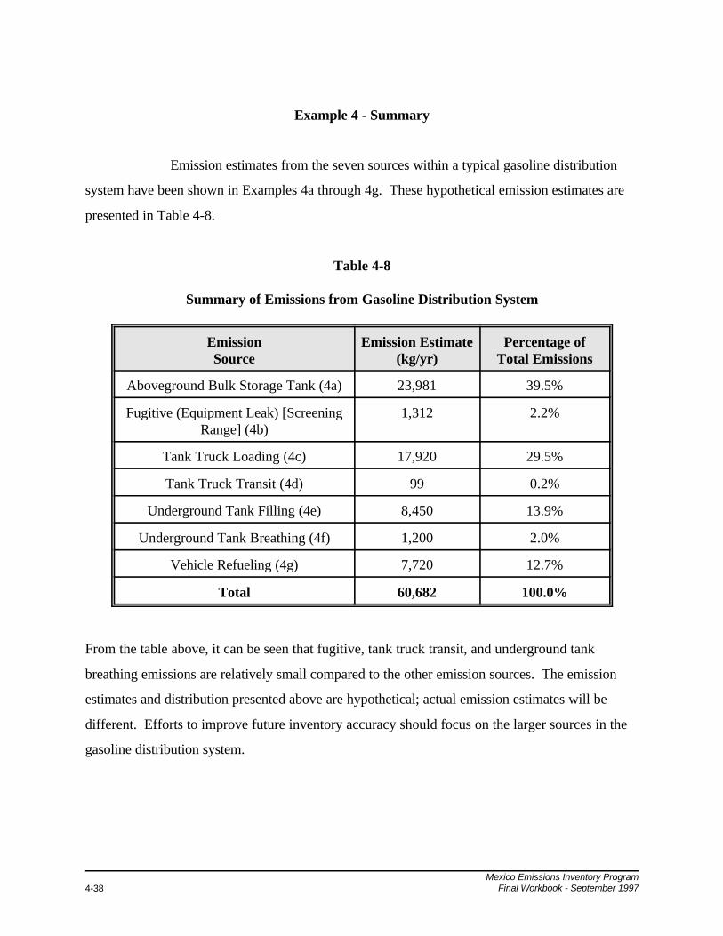
Mexico Emissions Inventory ProgramFinal Workbook - September 19974-38
Example 4 - Summary
Emission estimates from the seven sources within a typical gasoline distribution
system have been shown in Examples 4a through 4g. These hypothetical emission estimates are
presented in Table 4-8.
Table 4-8
Summary of Emissions from Gasoline Distribution System
EmissionSource
Emission Estimate(kg/yr)
Percentage ofTotal Emissions
Aboveground Bulk Storage Tank (4a) 23,981 39.5%
Fugitive (Equipment Leak) [ScreeningRange] (4b)
1,312 2.2%
Tank Truck Loading (4c) 17,920 29.5%
Tank Truck Transit (4d) 99 0.2%
Underground Tank Filling (4e) 8,450 13.9%
Underground Tank Breathing (4f) 1,200 2.0%
Vehicle Refueling (4g) 7,720 12.7%
Total 60,682 100.0%
From the table above, it can be seen that fugitive, tank truck transit, and underground tank
breathing emissions are relatively small compared to the other emission sources. The emission
estimates and distribution presented above are hypothetical; actual emission estimates will be
different. Efforts to improve future inventory accuracy should focus on the larger sources in the
gasoline distribution system.

Mexico Emissions Inventory ProgramFinal Workbook - September 1997 5-1
Example 5a
Solvent Evaporation - Degreasing
Introduction
Solvent degreasing or surface cleaning operations occur at a wide variety of
manufacturing, scientific, and repair facilities. Surface cleaning operations involve the use of
solvent liquids or vapors to remove water-insoluble contaminants such as grease, oils, waxes,
carbon deposits, fluxes, and tars from metal, plastic, glass, and other surfaces. Solvent degreasing
operations may involve the use of a number of different solvents, such as acetone, methyl ethyl
ketone (MEK), alcohols, 1,1,1-trichloroethane, or CFC-113.
Typical solvent cleaning equipment can be categorized as:
C Batch cold cleaning machines. These machines are batch loaded andliquid solvent is sprayed, dipped, or brushed onto the surfaces that are tobe cleaned.
C Batch vapor cleaning machines. These machines are batch loaded, andthe materials to be cleaned are exposed to vaporized solvent. Thecondensing solvent flushes the contaminants from the surfaces to becleaned.
C In-line cleaning machines. These machines are loaded using a conveyoron a continual basis and are often custom-made for large-scale operations. An in-line solvent cleaning machine may use liquid or vapor solvent.
Problem Statement
Estimate annual TOG emissions from a batch cold cleaning machine and a batch
vapor cleaning machine.

Mexico Emissions Inventory ProgramFinal Workbook - September 19975-2
Available Information
Batch cold cleaning machine
C Solvent used is aliphatic hydrocarbon (e.g., Stoddard solvent, petroleumnaphtha);
C Cold cleaner capacity is 200 liters;
C Solvent density is 0.8 g/ml (0.8 kg/liter);
C Solvent log data are shown in Table 5-1.
Table 5-1
Solvent Log Data
DateSolvent Added
(liters)Waste Liquid Removed
(liters)Waste Sludge Removed
(kg)
2 Feb 200 195 --
30 May 200 203 --
15 Aug 200 198 1.3
28 Nov 200 205 --
C Added fresh solvent is 100% TOG;
C Waste liquid is 95 wt% TOG (includes contaminants such as water, grease,oil, flux, etc.);
C Waste liquid is assumed to have the same density as fresh solvent;
C Solid waste (sludge) is 10 wt% TOG.

Mexico Emissions Inventory ProgramFinal Workbook - September 1997 5-3
Batch vapor cleaning machine
C Solvent used is perchloroethylene;
C Capacity is 200 liters;
C Solvent density is 1.6 g/ml (1.6 kg/liter);
C Solvent consumption data are shown in Table 5-2.
Table 5-2
Solvent Consumption Data
Date Solvent Added (liters)Waste Liquid Removed
(liters)Waste Sludge Removed
(kg)
14 Jan 20 -- --
8 Feb 35 -- --
26 Mar 200 178 --
10 Apr 20 -- --
2 May 25 -- --
18 May 20 -- --
20 Jun 200 160 --
4 Jul 15 -- --
6 Aug 30 -- --
18 Sep 200 167 2
3 Nov 50 -- --
15 Dec 200 185 --
C Fresh solvent is 100% TOG;
C Waste liquid is 95 wt% TOG (includes contaminants such as water, grease,oil, flux, etc.);
C Waste liquid is assumed to have the same density as fresh solvent; and
C Solid waste (sludge) is 10 wt% TOG.

Mexico Emissions Inventory ProgramFinal Workbook - September 19975-4
E ' (Qin × Din × TOGin) & (Qout(liq) × Dout(liq) × TOGout(liq)) & (Qout(solid) × TOGout(solid))
Solution
Emissions from cold cleaning occur through waste solvent and sludge evaporation,
solvent carryout or “dragout,” solvent bath evaporation, spray evaporation and agitation.
Emissions from vapor degreasing are due to diffusion and convection, solvent carryout or
“dragout,” exhaust systems, and waste solvent and sludge evaporation.
Since it would be very time- and cost-intensive to collect data on all of these loss
mechanisms, emission rates are usually estimated from solvent consumption data for the particular
degreasing operation under consideration. If solvent consumption data are not available, emission
factors based on number of employees or population data are available in literature (e.g., U.S.
EPA, 1991b). For point source emission calculations, it is highly recommended that the following
mass balance equation be used to estimate emissions:
where: E = Total TOG emissions (kg);Qin = Amount of solvent added to the degreaser (liters);Din = Density of solvent added to the degreaser (kg/liter);TOGin = TOG content of the solvent added to the degreaser (wt%);Qout(liq) = Amount of liquid waste removed from the degreaser (liters);Dout(liq) = Density of liquid waste removed from the degreaser
(kg/liter);TOGout(liq) = TOG content of liquid waste removed from the degreaser
(wt%);Qout(solid) = Amount of solid waste (sludge) removed from the degreaser
(kg); andTOGout(solid) = TOG content of solid waste (sludge) removed from the
degreaser (wt%).
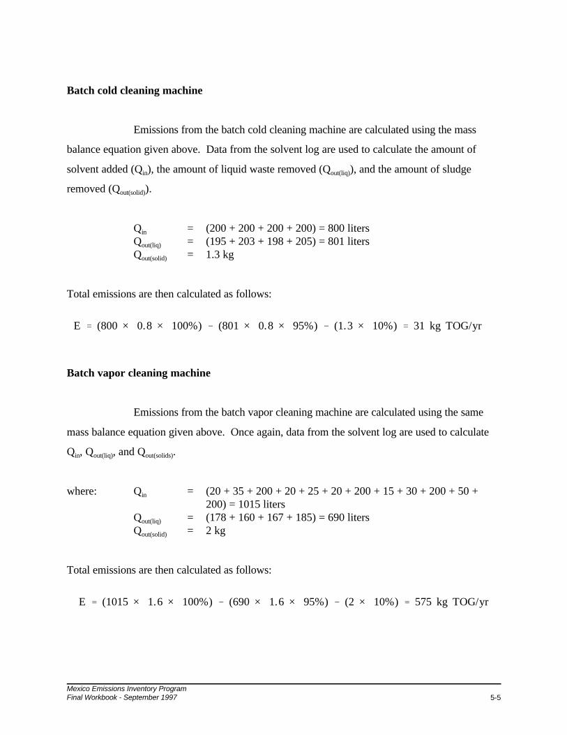
Mexico Emissions Inventory ProgramFinal Workbook - September 1997 5-5
E ' (800 × 0.8 × 100%) & (801 × 0.8 × 95%) & (1.3 × 10%) ' 31 kg TOG/yr
E ' (1015 × 1.6 × 100%) & (690 × 1.6 × 95%) & (2 × 10%) ' 575 kg TOG/yr
Batch cold cleaning machine
Emissions from the batch cold cleaning machine are calculated using the mass
balance equation given above. Data from the solvent log are used to calculate the amount of
solvent added (Qin), the amount of liquid waste removed (Qout(liq)), and the amount of sludge
removed (Qout(solid)).
Qin = (200 + 200 + 200 + 200) = 800 litersQout(liq) = (195 + 203 + 198 + 205) = 801 litersQout(solid) = 1.3 kg
Total emissions are then calculated as follows:
Batch vapor cleaning machine
Emissions from the batch vapor cleaning machine are calculated using the same
mass balance equation given above. Once again, data from the solvent log are used to calculate
Qin, Qout(liq), and Qout(solids).
where: Qin = (20 + 35 + 200 + 20 + 25 + 20 + 200 + 15 + 30 + 200 + 50 +200) = 1015 liters
Qout(liq) = (178 + 160 + 167 + 185) = 690 litersQout(solid) = 2 kg
Total emissions are then calculated as follows:

Mexico Emissions Inventory ProgramFinal Workbook - September 19975-6
The following issues should be considered when estimating emissions from solvent degreasing:
C Cold cleaner solvent consumption logs usually only include records ofchangeouts (i.e., all the liquid waste is removed and fresh solvent is addedfor the full cleaner capacity).
C Vapor degreaser consumption logs usually include records of changeoutsand replenishments (i.e., fresh solvent is added to replace evaporatedsolvent without any liquid waste being removed at the same time).
C The TOG content of the liquid and solid wastes should preferably bedetermined using periodic sampling. However, frequent sampling is usuallycost-prohibitive, so engineering judgement is often used to estimate theTOG content of liquid and solid wastes.
C The amount of TOG recovered in the solid waste (sludge) is usually verysmall compared to the amount of TOG recovered in the liquid waste. Therefore, it is often conservatively assumed that the TOG in the solidwaste is emitted to the air.
C Emissions from some degreasing solvents (e.g., perchloroethylene, freons,etc.) should not be included in ROG (reactive organic gas) inventories.
C Engineering judgement may be needed to reconcile the time period definedby the consumption log with the time period needed for the emissioncalculations. For example, the batch cold cleaner consumption log containsno data after 28 Nov, but the cold cleaner is still emitting until the end ofthe annual emission period (i.e., 31 Dec). For actual emission inventories,it is generally assumed that these additional emissions will be reflected atthe time of the next consumption entry (i.e., in the next calendar year).
Mexico Emissions Inventory ProgramFinal Workbook - September 1997 5-7
Example 5b
Solvent Evaporation - Surface Coating
Introduction
Surface coating includes all processes in which a liquid material is applied to the
surface of a solid substrate. Air emissions result from both the evaporation of the solvents or
other organic carriers in the coatings, and from the “overspray” of particulate materials that do
not adhere to each part. Particulate emissions can be reduced through the use of paint booths and
other control devices. In addition to the actual surface coating materials, emissions also result
from materials used for surface preparation prior to the application of surface coatings and for
cleanup afterwards.
Problem Statement
Estimate TOG, PM, and zinc compound emissions from the surface coating
operation described below. Include all surface coating, thinning, surface preparation, and cleanup
materials. There are no records that indicate the amount of paint used.
Available Information
Two types of paint (polyurethane and primer) are used. The polyurethane paint
consists of a base and a hardener that must be mixed together. In addition, the polyurethane paint
must be thinned with a thinner. The mixing ratio of the polyurethane is 7:2:1
(base:hardener:thinner). The primer does not have component parts and does not require
thinning. The material characteristics of the base, hardener, thinner, primer, and other surface
preparation and cleanup solvents are given in Table 5-3.

Mexico Emissions Inventory ProgramFinal Workbook - September 19975-8
Table 5-3
Surface Coating Material Characteristics
Material Density (grams/liter)VOC Content(grams/liter) Solids Content (%)
Polyurethane-base 700 520 31
Polyurethane-hardener 750 330 35
Polyurethane-thinner 820 820 -
Primer 680 460 40
Surface PreparationSolvent
820 820 -
Cleanup Solvent 820 820 -
Also, 2% of the solids of Paint 1 (as mixed) and 1.5% of the solids of Paint 2 are zinc compounds.
Half of the polyurethane is applied using high volume/low pressure (HVLP) spray
equipment, while the other half is applied using conventional spray equipment. The primer is
applied using aerosol spray cans. The polyurethane is used in a paint booth equipped with dry
particulate filters (approximate control efficiency [CE] of 90%), but the primer is used in an open
area.
The surface coating operation paints kitchen appliance parts. Annual throughput
of the operation is 25,000 parts. Painters working at the surface coating operation estimate that
each part requires 0.8 liters of polyurethane and 0.2 liters of primer. The painters also estimate
that the solvents used for surface preparation are 40% of the volume of paint applied on each
part, while cleanup solvents are 15% of the volume of paint applied. It is assumed that all surface
preparation and cleanup solvents are applied in a wipe application and that 100% of the applied
solvent evaporates. Only about 95% of polyurethane or primer in a given container can actually
be applied to the parts to be painted; the remaining 5% cannot be used. Nonetheless, it should be
assumed that all solvents in the waste paint evaporate to the atmosphere.
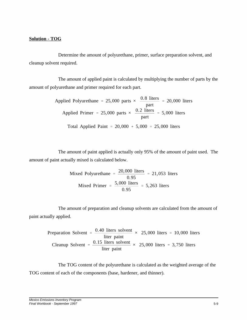
Mexico Emissions Inventory ProgramFinal Workbook - September 1997 5-9
Applied Polyurethane ' 25,000 parts × 0.8 literspart
' 20,000 liters
Applied Primer ' 25,000 parts × 0.2 literspart
' 5,000 liters
Total Applied Paint ' 20,000 % 5,000 ' 25,000 liters
Mixed Polyurethane '20,000 liters
0.95' 21,053 liters
Mixed Primer '5,000 liters
0.95' 5,263 liters
Preparation Solvent '0.40 liters solvent
liter paint× 25,000 liters ' 10,000 liters
Cleanup Solvent '0.15 liters solvent
liter paint× 25,000 liters ' 3,750 liters
Solution - TOG
Determine the amount of polyurethane, primer, surface preparation solvent, and
cleanup solvent required.
The amount of applied paint is calculated by multiplying the number of parts by the
amount of polyurethane and primer required for each part.
The amount of paint applied is actually only 95% of the amount of paint used. The
amount of paint actually mixed is calculated below.
The amount of preparation and cleanup solvents are calculated from the amount of
paint actually applied.
The TOG content of the polyurethane is calculated as the weighted average of the
TOG content of each of the components (base, hardener, and thinner).

Mexico Emissions Inventory ProgramFinal Workbook - September 19975-10
TOGpoly ' (%base × TOGbase) % (%hard × TOGhard) % (%thin × TOGthin)TOGpoly ' (0.7 × 520) % (0.2 × 330) % (0.1 × 820) ' 512 grams/liter
EmissionsPoly ' 21,053 liters × 512 gramsliter
' 10,779 kg
EmissionsPrimer ' 5,263 liters × 460 gramsliter
' 2,421 kg
EmissionsPrep ' 10,000 liters × 820 gramsliter
' 8,200 kg
EmissionsCleanup ' 3,750 liters × 820 gramsliter
' 3,075 kg
EmissionsTOG&Total ' 10,779 % 2,421 % 8,200 % 3,075 ' 24,475 kg ' 24.5 Mg
Emissionsi ' Pi × Di × SCi × (1 & 0)
Emissions are then calculated by multiplying the quantity of each paint or solvent
used by its respective TOG content.
Solution - PM
Uncontrolled PM emissions can be calculated using the following equation.
where: Emissionsi = Total uncontrolled emissions for surface coating, i (kg);Pi = Amount of paint applied (liter);Di = Density of surface coating, i (g/liter);SCi = Solids content of surface coating, i (fraction); and0 = Transfer efficiency of application method (fraction).
First, the density and solids content of the polyurethane paint needs to be
determined. Density and solids content information are taken from the material characteristics
table.

Mexico Emissions Inventory ProgramFinal Workbook - September 1997 5-11
Dpoly ' (%base × Dbase) % (%hard × Dhard) % (%thin × Dthin)
Dpoly ' 0.7 × 700 % 0.2 × 750 % 0.1 × 820 ' 722 grams/liter
SCpoly 'DbaseSCbase%base % DhardSChard%hard % DthinSCthin%thin
Dpoly
SCTot '(700)(0.31)(0.70) % (750)(0.35)(0.20) %(820)(0.00)(0.10)
722' 28.3%
Transfer efficiencies for various application methods are presented in Table 5-4.
Table 5-4
Surface Coating Transfer Efficiencies
Application Method Transfer Efficiency
Aerosol Spray Can 0.24
Airless Spray Equipment 0.35
Brush or Roller 0.95
Conventional Air Spray Equipment 0.30
High Volume/Low Pressure (HVLP)Spray Equipment
0.60
Source: SCAQMD, 1996

Mexico Emissions Inventory ProgramFinal Workbook - September 19975-12
EmissionsPoly,HVLP '722 grams
liter× 0.283 × (1 & 0.60) × 10,000 liters ' 817 kg
EmissionsPoly,other '722 grams
liter× 0.283 × (1 & 0.30) × 10,000 liters ' 1,430 kg
EmissionsPrimer '680 grams
liter× 0.4 × (1 & 0.24) × 5,000 liters ' 1,034 kg
EmissionsPoly,cont ' (1 & CE) (EmissionsPoly,HVLP % EmissionsPoly,other)
EmissionsPoly,cont ' (1 & 0.90) (817 % 1,430) ' 225 kg
EmissionsTotal ' 225 % 1,034 ' 1,259 kg ' 1.3 Mg
EmissionsZn,poly ' 2% × 225 kg PM10 ' 4.5 kgEmissionsZn,primer ' 1.5% × 1,034 kg PM10 ' 15.5 kg
EmissionsZn,total ' 4.5 % 15.5 ' 20 kg
Uncontrolled PM emissions are calculated below.
The controlled PM emissions for the polyurethane are calculated below.
where: CE = control efficiency
Finally, total combined PM emissions for the polyurethane and the primer are calculated.
Solution - Zinc Compounds
Emissions of a specific species are simply calculated by multiplying overall PM
emissions by the percentage of that specific species. Using this method, zinc compound emissions
are calculated below.

Mexico Emissions Inventory ProgramFinal Workbook - September 1997 6-1
Example 6
Point Source Stack Emissions
Introduction
Among the various emission estimating techniques, source sampling provides the
most reliable emission estimates (although the costs also tend to be the highest). The reason for
the high accuracy is that the effects of equipment- and process-specific parameters are actually
being measured by the sampling equipment. Although source sampling can provide accurate
emission estimates, sometimes much effort is required to convert sampling data into emission
estimates. This example demonstrates the process of converting concentration measurements into
mass emission rates.
Problem Statement
Determine the average hourly and annual emissions of NOx from a process stack
given typical stack measurements.
Available Information
The following average measurements have been collected from the stack through
approved source testing methods:
Actual stack gas flow rate: 7486 cfm
Stack gas temperature:80.0EC
Stack diameter:0.75 m
Water vapor content: 2.1%vol
CO2 content:9.5%vol

Mexico Emissions Inventory ProgramFinal Workbook - September 19976-2
'7486 ft 3
min0.3048 m
ft
3
' 2.12 × 10² m 3
minat 80EC, stack pressure
NOx concentration:48 ppmv
The remainder of the stack gas should be assumed to be air. The process operates
24 hours per day, 330 days per year.
Solution
The steps necessary to determine the daily and annual NOx emissions from this
process stack with the information provided are:
1. Collect the data needed for stack gas calculations and define terms:
Standard molar volume (Vs) (at 20EC): 0.024 m3/g-moleMolecular weight (MW) of NOx: 46 (NOx is expressed as NO2 by
convention)Standard conditions: 20EC and 760 mmHg
Standard conditions (temperature and pressure) are often used so that allemissions are reported on the same basis. Different standard conditionsmay apply in different jurisdictions and for different applications.
2. Determine the metric flow rate of the stack gas (volume/unit time) at stackconditions (m3/min):
a. Given:
Actual stack gas flow rate: 7486 cfmStack temperature: 80.0EC
b. Metric flow rate of stack gas at stack conditions:

Mexico Emissions Inventory ProgramFinal Workbook - September 1997 6-3
Qdry ' Qwet
Vdry
Vwet
'2.12 × 10² m 3 stack gas (wet)
min(1 & 0.021) m 3 stack gas (dry)
1 m 3 stack gas (wet)
'2.08 × 10² m 3 stack gas (dry)
min
3. Determine the volumetric flow rate of NOx in the stack gas (volume/unittime):
a. The stack gas in this example is wet (2.1% water by volume). Theinformation given does not specify if the NOx concentration wasmeasured on a wet basis or a dry basis. However, from knowledgeof analytical techniques, it is known that NOx measurements aremade and reported on a dry basis, therefore the dry stack gas flowrate must first be calculated.
b. Calculate the dry stack gas volumetric flow rate:
1. Given:
Stack gas water content: 2.1% by volumeWet stack gas flow rate: 2.12 × 10² m3/min
(at 80EC, stack pressure)
2. Dry stack gas flow rate:
where: Qdry = dry stack gas flow rate;Qwet = wet stack gas flow rate; andVdry/Vwet = fraction of air in wet stack gas.

Mexico Emissions Inventory ProgramFinal Workbook - September 19976-4
2.08 × 10² m 3 stack gasmin
48 m 3 NOx
106 m 3 stack gas'
9.98 × 10&3 m 3 NOx
minat 80EC, stack pressure, dry basis
c. Calculate NOx flow rate:
1. Given:
NOx concentration: 48 ppmv
2. NOx flow rate:
QNOx = QdryCNOx
where: QNOx = NOx flow rate;Qdry = dry stack gas flow rate; andCNOx = NOx concentration
4. Correct the volumetric flow rate of NOx to standard conditions (20EC and760 mmHg) using the ideal gas law.
a. For this example, it is assumed that correction is required only fortemperature because the stack gas is assumed to be at 1 atmosphere(760 mmHg) due to the stack being open to the atmosphere at sealevel.
b. From the ideal gas law (PV = nRT), the relationship between gasvolume and gas temperature is:
V = nRT/PV/T = nR/P
c. In this example, regardless of the temperature of the stack, thenumber of moles (n) of the NOx in the stack gas, gas constant (R),and pressure (P) of the stack gas are constant. Therefore, therelationship between gas volume and gas temperature can bedeveloped as follows for any two absolute temperatures (T1 and T2):
V1/T1 = n1R1/P1 and V2/T2 = n2R2/P2

Mexico Emissions Inventory ProgramFinal Workbook - September 1997 6-5
Q2 ' 9.96 × 10&3m 3 NOx
min[20EC % 273][80EC % 273]
' 8.27 × 10&3 Sm 3 (standard cubic meter)min
at 20EC, 760 mmHg
Volumetric flow rate of NOx ' 8.27 × 10&3 Sm 3
min
Vs standard molar volume ' 0.024 Sm 3
g&mole20EC, 760 mmHg
MW of NOx as NO2 ' 46 gg&mole
Annual stack operation ' 24 hours per day, 330 days per year
Since nR/P is constant, then n1R1/P1 = n2R2/P2, therefore:
V1/T1 = V2/T2
d. Solving for the unknown gas volume (V2) at the new temperature(T2),
V2 = V1T2/T1
e. The equation for the unknown volume flow rate (Q2) at the newtemperature (T2) is similar,
Q2 = Q1T2/T1
f. Calculate the volume flow rate of NOx (Q2) at the new temperature(20EC) (absolute temperatures must be used in this calculation):
5. Determine mass flow rate and daily and annual NOx emissions (mass/dayand mass/year):
a. Given:

Mexico Emissions Inventory ProgramFinal Workbook - September 19976-6
MNOx'
QNOxMWNOx
VS
8.27 × 10&3Sm 3 NOx
min
1 g&mole NOx
0.024 Sm 3 NOx
46 g NOx
g&mole NOx
' 15.8g NOx
min
15.8 g NOx
min60 min
1 hr1 kg
103 g' 0.948
kg NOx
hr
0.948 kg NOx
hr24 hrday
330 daysyr
' 7.51 × 10³ kg/yr
' 7.5 Mg/yr
b. Mass flow rate of NOx:
where: MNOx = NOx mass flow rate;QNOx = NOx volumetric flow rate;MWNOx = NOx molecular weight; andVs = standard molar volume
c. Hourly emissions:
d. Annual emissions:

Mexico Emissions Inventory ProgramFinal Workbook - September 1997 7-1
Example 7
Particulate Matter - Estimation of PM10, PM2.5, OC, and EC
Introduction
Particulate emissions consist of particles with a wide range of sizes. They range in
size from near molecular dimensions to 100 microns in diameter. Particles with diameters greater
than 100 microns do not stay suspended for any significant period of time and settle out near their
point of origin. Consequently, these particles are usually not considered in air quality
applications. Currently, most inventory efforts focus on PM10 (particulate matter with an
aerodynamic diameter of less than or equal to 10 microns). However, as the focus of air quality
has grown to include visibility issues, more attention has been given to PM2.5 (particulate matter
with an aerodynamic diameter of less than or equal to 2.5 microns) emissions. Visibility-related
research also requires an analysis of particulate composition. The amount of light extinction
caused by particulate matter is a function of its chemical composition. Particulate matter
containing organic carbon (OC) or elemental carbon (EC) absorbs light; whereas, particulate
matter containing other chemical compounds tends to scatter light.
Problem Statement
Estimate PM10, PM2.5, OC, and EC emissions given total suspended particulate
(TSP) emissions from paved and unpaved roads.
Available Information
Using standard estimating methodologies, it has been estimated that TSP emissions
are 600 Mg for paved roads and 3,000 Mg for unpaved roads within a particular inventory
domain.
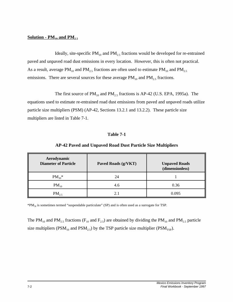
Mexico Emissions Inventory ProgramFinal Workbook - September 19977-2
Solution - PM10 and PM2.5
Ideally, site-specific PM10 and PM2.5 fractions would be developed for re-entrained
paved and unpaved road dust emissions in every location. However, this is often not practical.
As a result, average PM10 and PM2.5 fractions are often used to estimate PM10 and PM2.5
emissions. There are several sources for these average PM10 and PM2.5 fractions.
The first source of PM10 and PM2.5 fractions is AP-42 (U.S. EPA, 1995a). The
equations used to estimate re-entrained road dust emissions from paved and unpaved roads utilize
particle size multipliers (PSM) (AP-42, Sections 13.2.1 and 13.2.2). These particle size
multipliers are listed in Table 7-1.
Table 7-1
AP-42 Paved and Unpaved Road Dust Particle Size Multipliers
AerodynamicDiameter of Particle Paved Roads (g/VKT) Unpaved Roads
(dimensionless)
PM30* 24 1
PM10 4.6 0.36
PM2.5 2.1 0.095
*PM30 is sometimes termed “suspendable particulate” (SP) and is often used as a surrogate for TSP.
The PM10 and PM2.5 fractions (F10 and F2.5) are obtained by dividing the PM10 and PM2.5 particle
size multipliers (PSM10 and PSM2.5) by the TSP particle size multiplier (PSMTSP).

Mexico Emissions Inventory ProgramFinal Workbook - September 1997 7-3
F10&paved 'PSM10&paved
PSMTSP&paved
'4.624
' 0.192
F2.5&paved 'PSM2.5&paved
PSMTSP&paved
'2.124
' 0.088
F10&unpaved 'PSM10&unpaved
PSMTSP&unpaved
'0.36
1' 0.360
F2.5&unpaved 'PSM2.5&unpaved
PSMTSP&unpaved
'0.095
1' 0.095
Another source of PM10 and PM2.5 fractions is EPA’s SPECIATE database (U.S. EPA, 1992).
The SPECIATE database contains speciation profiles for a wide range of emission categories.
Many of these profiles are composite profiles. In addition, mass fractions for different size
intervals are given for each emission category. Based on composite profiles, the PM10 and PM2.5
fractions (F10 and F2.5) for paved and unpaved roads are given in Table
7-2.
Table 7-2
SPECIATE Paved and Unpaved Road Dust Mass Fractions
Particle Size Interval (µm)Paved Road Fraction
(SPECIATE profile 41130)Unpaved Road Fraction
(SPECIATE profile 41220)
0-2.5 0.25 0.3
0-10 0.44 0.73
Similarly, the California Air Resources Board provides its own mass fractions for different size
intervals (ARB, 1996). These are given in Table 7-3.

Mexico Emissions Inventory ProgramFinal Workbook - September 19977-4
F2.5 ' F<1 % F1&2.5 ' 0.03 % 0.05 ' 0.08F10 ' F<1 % F1&2.5 %F2.5&10 ' 0.03 % 0.05 % 0.38 ' 0.46
F2.5 ' F<1 % F1&2.5 ' 0.05 % 0.08 ' 0.13F10 ' F<1 % F1&2.5 % F2.5&10 ' 0.05 % 0.08 % 0.49 ' 0.62
Emissionsi ' EmissionsTSP × Fi
Table 7-3
ARB Paved and Unpaved Road Dust Mass Fractions
Particle Size Interval (µm) Paved Road Fraction Unpaved Road Fraction
<1 0.03 0.05
1-2.5 0.05 0.08
2.5-10 0.38 0.49
>10 0.54 0.38
Because the mass fractions do not correspond to PM10 and PM2.5 fractions, certain mass fractions
must be summed together as demonstrated below.
For paved roads:
For unpaved roads:
After obtaining PM10 and PM2.5 fractions, PM10 and PM2.5 emissions are then calculated using the
following equation.
where: Emissionsi = Emissions of aerodynamic diameter less than i microns;EmissionsTSP = Emissions of total suspended particulate matter; andFi = Fraction of total suspended particulate matter of
aerodynamic diameter less than i microns.
Because generic PM10 and PM2.5 fractions are being used rather than site-specific fractions, PM10
and PM2.5 emissions will be estimated using PM10 and PM2.5 fractions from each of the three
sources presented above. In addition, the average of the three PM10 and PM2.5 fractions is used to

Mexico Emissions Inventory ProgramFinal Workbook - September 1997 7-5
estimate PM10 and PM2.5 emissions. All four of the estimates are presented in Table 7-4. It
should be noted that none of these estimates have been identified as being better or more accurate
than the others. There is still considerable uncertainty associated with paved and unpaved road
emission estimates. Research is underway to improve the existing methodologies for these source
categories. This example simply demonstrates how to derive PM10 and PM2.5 estimates from TSP
emissions.
Table 7-4
PM10 and PM2.5 Emissions Calculated Using Different Size Fractions
RoadType Pollutant
Source ofFraction Size Fraction
TSP(Mg/yr)
Emissions(Mg/yr)
Paved PM10 AP-42 0.192 600 115.2
SPECIATE 0.44 264
ARB 0.46 276
Average 0.364 218.4
PM2.5 AP-42 0.088 600 52.8
SPECIATE 0.25 150
ARB 0.08 48
Average 0.139 83.4
Unpaved PM10 AP-42 0.36 3,000 1,080
SPECIATE 0.73 2,190
ARB 0.62 1,860
Average 0.57 1,710
PM2.5 AP-42 0.095 3,000 285
SPECIATE 0.30 900
ARB 0.13 390
Average 0.175 525

Mexico Emissions Inventory ProgramFinal Workbook - September 19977-6
Solution - OC and EC
Like PM10 and PM2.5 fractions, site-specific OC and EC fractions should be
developed whenever possible in order to obtain the most accurate emission estimates. In some
instances, however, detailed laboratory analysis is not possible. Generic speciation profiles must
then be used. A source for generic speciation profiles is EPA’s SPECIATE database. These
SPECIATE speciation profiles indicate the percentage of individual compounds relative to overall
particulate matter emissions. For paved and unpaved road dust, these speciation profiles include
various metal species, in addition to OC and EC.
Hypothetical sampling data gives the following OC and EC fractions for paved and
unpaved roads. Three samples were taken for both paved and unpaved roads. Two size fractions
were sampled - fine (0-2.5 µm) and coarse (2.5-10 µm). These data are presented in Table 7-5.
Table 7-5
Hypothetical OC and EC Sampling Data
Road Type Sample Size Fraction OC fraction (wt%) EC fraction (wt%)Paved #1 Fine 17.27 0.72
Coarse 12.35 0.44#2 Fine 19.41 0.45
Coarse 10.89 0.60#3 Fine 18.54 0.63
Coarse 11.37 0.53Average Fine 18.41 0.60
Coarse 11.54 0.52Unpaved #1 Fine 2.46 0.00
Coarse 1.50 0.00#2 Fine 2.71 0.00
Coarse 1.65 0.00#3 Fine 2.77 0.00
Coarse 1.29 0.00Average Fine 2.65 0.00
Coarse 1.48 0.00

Mexico Emissions Inventory ProgramFinal Workbook - September 1997 7-7
Fi ' (Fi,c × %c) % (Fi,f × %f)
FOC,paved ' (11.54 × 0.54) % (18.41 × 0.46) ' 14.70FEC,paved ' (0.52 × 0.54) % (0.60 × 0.46) ' 0.56
FOC,unpaved ' (1.48 × 0.35) % (2.65 × 0.65) ' 2.24FEC,unpaved ' (0.00 × 0.35) % (0.00 × 0.65) ' 0.00
The OC and EC fractions (FOC and FEC) for PM2.5 can be taken directly from the table above
because fine particulate is defined as PM2.5. The OC and EC fractions for PM10 must be
calculated using a weighted average of fine and coarse OC and EC fractions. Additional sampling
data (not included in the table on the previous page) indicates that paved road dust PM10 consists
of 54 wt% coarse particulate and 46 wt% fine particulate, whereas unpaved road dust PM10
consists of 35 wt% coarse particulate and 65 wt% fine particulate. The weighted OC and EC
fractions for PM10 are calculated using the following equation.
where Fi = Overall fraction of species i;Fi,c = Fraction of species i in coarse portion of particulate;%c = Weight percent of coarse particulate;Fi,f = Fraction of species i in fine portion of particulate; and%f = Weight percent of fine particulate.
The weighted PM10 OC and EC fractions are calculated below for both paved and unpaved roads.
OC and EC emissions are calculated in Table 7-6. PM10 and PM2.5 emissions are
assumed to be equal to the average values calculated earlier.

Mexico Emissions Inventory ProgramFinal Workbook - September 19977-8
Table 7-6
Calculated OC and EC Emissions
RoadType Pollutant
Emissions(Mg/yr)
OCFraction
OC Emissions(Mg/yr)
ECFraction
EC Emissions(Mg/yr)
Paved PM10 218.4 0.1470 32.1 0.0056 1.2
PM2.5 83.4 0.1841 15.4 0.0060 0.5
Unpaved PM10 1710 0.0224 38.3 0.0000 0.0
PM2.5 525 0.0265 13.9 0.0000 0.0

APPENDIX A
MISCELLANEOUS DATA AND CONVERSION FACTORS
(Information in this appendix is taken from AP-42, Appendix A. Fuel parameters are for U.S.fuels; Mexico fuels are likely to differ and should be examined carefully.)

Mexico Emissions Inventory ProgramFinal Workbook - September 1997 A-1
SOME USEFUL WEIGHTS AND MEASURES
Unit Of Measure Equivalentgrain 0.002 ounces
gram 0.04 ounces
ounce 28.35 grams
kilogram 2.21 pounds
pound 0.45 kilograms
pound (troy) 12 ounces
ton (short) 2000 pounds
ton (long) 2240 pounds
ton (metric) 2200 pounds
ton (shipping) 40 feet3
centimeter 0.39 inches
inch 2.54 centimeters
foot 30.48 centimeters
meter 1.09 yards
yard 0.91 meters
mile 1.61 kilometers
centimeter2 0.16 inches2
inch2 6.45 centimeters2
foot2 0.09 meters2
meter2 1.2 yards2
yard2 0.84 meters2
mile2 2.59 kilometers2
centimeter3 0.061 inches3
inch3 16.39 centimeters3
foot3 283.17 centimeters3
foot3 1728 inches3

SOME USEFUL WEIGHTS AND MEASURES (cont.)
Unit Of Measure Equivalent
Mexico Emissions Inventory ProgramFinal Workbook - September 1997A-2
meter3 1.31 yeads3
yard3 0.77 meters3
cord 128 feet3
cord 4 meters3
peck 8 quarts
bushel (dry) 4 pecks
bushel 2150.4 inches3
gallon (U. S.) 231 inches3
barrel 31.5 gallons
hogshead 2 barrels
township 36 miles2
hectare 2.5 acres
MISCELLANEOUS DATA
One cubic foot of anthracite coal weighs about 53 pounds.
One cubic foot of bituminous coal weighs from 47 to 50 pounds.
One ton of coal is equivalent to two cords of wood for steam purposes.
A gallon of water (U. S. Standard) weighs 8.33 pounds and contains 231 cubic inches.
There are 9 square feet of heating surface to each square foot of grate surface.
A cubic foot of water contains 7.5 gallons and 1728 cubic inches, and weighs 62.5 lbs.
Each nominal horsepower of a boiler requires 30 to 35 pounds of water per hour.
A horsepower is equivalent to raising 33,000 pounds one foot per minute, or 550 pounds one foot persecond.
To find the pressure in pounds per square inch of a column of water, multiply the height of the column infeet by 0.434.

Mexico Emissions Inventory ProgramFinal Workbook - September 1997 A-3
TYPICAL PARAMETERS OF VARIOUS FUELSa
Type Of Fuel
Heating ValueSulfur
% (by weight)
Ash% (byweight)kcal Btu
Solid Fuels
Bituminous Coal 7,200/kg 13,000/lb 0.6-5.4 4-20
Anthracite Coal 6,810/kg 12,300/lb 0.5-1.0 7.0-16.0
Lignite (@ 35% moisture) 3,990/kg 7,200/lb 0.7 6.2
Wood (@ 40% moisture) 2,880/kg 5,200/lb N 1-3
Bagasse (@ 50% moisture) 2,220/kg 4,000/lb N 1-2
Bark (@ 50% moisture) 2,492/kg 4,500/lb N 1-3b
Coke, Byproduct 7,380/kg 13,300/lb 0.5-1.0 0.5-5.0
Liquid Fuels
Residual Oil 9.98 x 10⁶/m3 150,000/gal 0.5-4.0 0.05-0.1
Distillate Oil 9.30 x 10⁶/m3 140,000/gal 0.2-1.0 N
Diesel 9.12 x 10⁶/m3 137,000/gal 0.4 N
Gasoline 8.62 x 10⁶/m3 130,000/gal 0.03-0.04 N
Kerosene 8.32 x 10⁶/m3 135,000/gal 0.02-0.05 N
Liquid Petroleum Gas 6.25 x 10⁶/m3 94,000/gal N N
Gaseous Fuels
Natural Gas 9,341/m3 1,050/SCF N N
Coke Oven Gas 5,249/m3 590/SCF 0.5-2.0 N
Blast Furnace Gas 890/m3 100/SCF N Na N = negligible.b Ash content may be considerably higher when sand, dirt, etc., are present.

Mexico Emissions Inventory ProgramFinal Workbook - September 1997A-4
THERMAL EQUIVALENTS FOR VARIOUS FUELS
Type Of Fuel kcal Btu (gross)
Solid fuels
Bituminous coal (5.8 to 7.8) x 106/Mg (21.0 to 28.0) x 106/ton
Anthracite coal 7.03 x 10⁶/Mg 25.3 x 10⁶/ton
Lignite 4.45 x 10⁶/Mg 16.0 x 10⁶/ton
Wood 1.47 x 10⁶/m3 21.0 x 10⁶/cord
Liquid fuels
Residual fuel oil 10 x 103/liter 6.3 x 10⁶/bbl
Distillate fuel oil 9.35 x 10³/liter 5.9 x 10⁶/bbl
Gaseous fuels
Natural gas 9,350/m3 1,050/ft3
Liquefied petroleum gas
Butane 6,480/liter 97,400/gal
Propane 6,030/liter 90,500/gal
WEIGHTS OF SELECTED SUBSTANCES
Type Of Substance g/liter lb/gal
Asphalt 1030 8.57
Butane, liquid at 60EF 579 4.84
Crude oil 850 7.08
Distillate oil 845 7.05
Gasoline 739 6.17
Propane, liquid at 60EF 507 4.24
Residual oil 944 7.88
Water 1000 8.4

Mexico Emissions Inventory ProgramFinal Workbook - September 1997 A-5
DENSITIES OF SELECTED SUBSTANCES
Substance DensityFuels
Crude Oil 874 kg/m3 7.3 lb/gal
Residual Oil 944 kg/m3 7.88 lb/gal
Distillate Oil 845 kg/m3 7.05 lb/gal
Gasoline 739 kg/m3 6.17 lb/gal
Natural Gas 673 kg/m3 1 lb/23.8 ft3
Butane 579 kg/m3 4.84 lb/gal (liquid)
Propane 507 kg/m3 4.24 lb/gal (liquid)
Wood (Air dried)
Elm 561 kg/m3 35 lb/ft3
Fir, Douglas 513 kg/m3 32 lb/ft3
Fir, Balsam 400 kg/m3 25 lb/ft3
Hemlock 465 kg/m3 29 lb/ft3
Hickory 769 kg/m3 48 lb/ft3
Maple, Sugar 689 kg/m3 43 lb/ft3
Maple, White 529 kg/m3 33 lb/ft3
Oak, Red 673 kg/m3 42 lb/ft3
Oak, White 769 kg/m3 48 lb/ft3
Pine, Southern 641 kg/m3 40 lb/ft3
Agricultural Products
Corn 25.4 kg/bu 56 lb/bu
Milo 25.4 kg/bu 56 lb/bu
Oats 14.5 kg/bu 32 lb/bu
Barley 21.8 kg/bu 48 lb/bu
Wheat 27.2 kg/bu 60 lb/bu
Cotton 226 kg/bale 500 lb/bale
Mineral Products
Brick 2.95 kg/brick 6.5 lb/brick
Cement 170 kg/bbl 375 lb/bbl
Cement 1483 kg/m3 2500 lb/yd3
Concrete 2373 kg/m3 4000 lb/yd3
Glass, Common 2595 kg/m3 162 lb/ft3
Gravel, Dry Packed 1600 - 1920 kg/m3 100 - 120 lb/ft3
Gravel, Wet 2020 kg/m3 126 lb/ft3
Gypsum, Calcined 880 - 960 kg/m3 55 - 60 lb/ft3
Lime, Pebble 850 - 1025 kg/m3 53 - 64 lb/ft3
Sand, Gravel (Dry, loose) 1440 - 1680 kg/m3 90 - 105 lb/ft3

Mexico Emissions Inventory ProgramFinal Workbook - September 1997A-6
CONVERSION FACTORS
The table of conversion factors on the following pages contains factors for converting English tometric units and metric to English units as well as factors to manipulate units within the same system. Thefactors are arranged alphabetically by unit within the following property groups.
- Area- Density- Energy- Force- Length- Mass- Pressure- Velocity- Volume- Volumetric Rate
To convert a number from one unit to another:
1. Locate the unit in which the number is currently expressed in the left-hand column of the table;
2. Find the desired unit in the center column; and
3. Multiply the number by the corresponding conversion factor in the right-hand column.

Mexico Emissions Inventory ProgramFinal Workbook - September 1997 A-7
CONVERSION FACTORSa
To Convert From To Multiply ByArea
Acres Sq feet 4.356 x 10⁴
Acres Sq kilometers 4.0469 x 10⁻³
Acres Sq meters 4.0469 x 10³
Acres Sq miles (statute) 1.5625 x 10⁻³
Acres Sq yards 4.84 x 10³
Sq feet Acres 2.2957 x 10⁻⁵
Sq feet Sq cm 929.03
Sq feet Sq inches 144.0
Sq feet Sq meters 0.092903
Sq feet Sq miles 3.587 x 10⁻⁸
Sq feet Sq yards 0.111111
Sq inches Sq feet 6.9444 x 10⁻³
Sq inches Sq meters 6.4516 x 10⁻⁴
Sq inches Sq mm 645.16
Sq kilometers Acres 247.1
Sq kilometers Sq feet 1.0764 x 10⁷
Sq kilometers Sq meters 1.0 x 10⁶
Sq kilometers Sq miles 0.386102
Sq kilometers Sq yards 1.196 x 10⁶
Sq meters Sq cm 1.0 x 10⁴
Sq meters Sq feet 10.764
Sq meters Sq inches 1.55 x 10³
Sq meters Sq kilometers 1.0 x 10⁻⁶
Sq meters Sq miles 3.861 x 10⁻⁷
Sq meters Sq mm 1.0 x 10⁶
Sq meters Sq yards 1.196
Sq miles Acres 640.0
Sq miles Sq feet 2.7878 x 10⁷
Sq miles Sq kilometers 2.590

CONVERSION FACTORS (cont.)
To Convert From To Multiply By
Mexico Emissions Inventory ProgramFinal Workbook - September 1997A-8
Sq miles Sq meters 2.59 x 10⁶
Sq miles Sq yards 3.0976 x 10⁶
Sq yards Acres 2.0661 x 10⁻⁴
Sq yards Sq cm 8.3613 x 10³
Sq yards Sq ft 9.0
Sq yards Sq inches 1.296 x 10³
Sq yards Sq meters 0.83613
Sq yards Sq miles 3.2283 x 10⁻⁷
Density
Dynes/cu cm Grams/cu cm 1.0197 x 10⁻³
Grains/cu foot Grams/cu meter 2.28835
Grams/cu cm Dynes/cu cm 980.665
Grams/cu cm Grains/milliliter 15.433
Grams/cu cm Grams/milliliter 1.0
Grams/cu cm Pounds/cu inch 1.162
Grams/cu cm Pounds/cu foot 62.428
Grams/cu cm Pounds/cu inch 0.036127
Grams/cu cm Pounds/gal (Brit.) 10.022
Grams/cu cm Pounds/gal (U. S., dry) 9.7111
Grams/cu cm Pounds/gal (U. S., liq.) 8.3454
Grams/cu meter Grains/cu foot 0.4370
Grams/liter Pounds/gal (U. S.) 8.345 x 10⁻³
Kilograms/cu meter Grams/cu cm 0.001
Kilograms/cu meter Pounds/cu ft 0.0624
Kilograms/cu meter Pounds/cu in 3.613 x 10⁻⁵
Pounds/cu foot Grams/cu cm 0.016018
Pounds/cu foot kg/cu meter 16.018
Pounds/cu inch Grams/cu cm 27.68
Pounds/cu inch Grams/liter 27.681
Pounds/cu inch kg/cu meter 2.768 x 10⁴

CONVERSION FACTORS (cont.)
To Convert From To Multiply By
Mexico Emissions Inventory ProgramFinal Workbook - September 1997 A-9
Pounds/gal (U. S., liq.) Grams/cu cm 0.1198
Pounds/gal (U. S., liq.) Pounds/cu ft 7.4805
Energy
Btu Cal. gm (IST.) 251.83
Btu Ergs 1.05435 x 10¹⁰
Btu Foot-pounds 777.65
Btu Hp-hours 3.9275 x 10⁻⁴
Btu Joules (Int.) 1054.2
Btu kg-meters 107.51
Btu kW-hours (Int.) 2.9283 x 10⁻⁴
Btu/hr Cal. kg/hr 0.252
Btu/hr Ergs/sec 2.929 x 10⁶
Btu/hr Foot-pounds/hr 777.65
Btu/hr Horsepower (mechanical) 3.9275 x 10⁻⁴
Btu/hr Horsepower (boiler) 2.9856 x 10⁻⁵
Btu/hr Horsepower (electric) 3.926 x 10⁻⁴
Btu/hr Horsepower (metric) 3.982 x 10⁻⁴
Btu/hr Kilowatts 2.929 x 10⁻⁴
Btu/lb Foot-pounds/lb 777.65
Btu/lb Hp-hr/lb 3.9275 x 10⁻⁴
Btu/lb Joules/gram 2.3244
Calories, kg (mean) Btu (IST.) 3.9714
Calories, kg (mean) Ergs 4.190 x 10¹⁰
Calories, kg (mean) Foot-pounds 3.0904 x 10³
Calories, kg (mean) Hp-hours 1.561 x 10⁻³
Calories, kg (mean) Joules 4.190 x 10³
Calories, kg (mean) kg-meters 427.26
Calories, kg (mean) kW-hours (Int.) 1.1637 x 10⁻³
Ergs Btu 9.4845 x 10⁻¹¹
Ergs Foot-poundals 2.373 x 10⁻⁶

CONVERSION FACTORS (cont.)
To Convert From To Multiply By
Mexico Emissions Inventory ProgramFinal Workbook - September 1997A-10
Ergs Foot-pounds 7.3756 x 10⁻⁸
Ergs Joules (Int.) 9.99835 x 10⁻⁸
Ergs kW-hours 2.7778 x 10⁻¹⁴
Ergs kg-meters 1.0197 x 10⁻⁸
Foot-pounds Btu (IST.) 1.2851 x 10⁻³
Foot-pounds Cal. kg (IST.) 3.2384 x 10⁻⁴
Foot-pounds Ergs 1.3558 x 10⁷
Foot-pounds Foot-poundals 32.174
Foot-pounds Hp-hours 5.0505 x 10⁻⁷
Foot-pounds Joules 1.3558
Foot-pounds kg-meters 0.138255
Foot-pounds kW-hours (Int.) 3.76554 x 10⁻⁷
Foot-pounds Newton-meters 1.3558
Foot-pounds/hr Btu/min 2.1432 x 10⁻⁵
Foot-pounds/hr Ergs/min 2.2597 x 10⁵
Foot-pounds/hr Horsepower (mechanical) 5.0505 x 10⁻⁷
Foot-pounds/hr Horsepower (metric) 5.121 x 10⁻⁷
Foot-pounds/hr Kilowatts 3.766 x 10⁻⁷
Horsepower (mechanical) Btu (mean)/hr 2.5425 x 10³
Horsepower (mechanical) Ergs/sec 7.457 x 10⁹
Horsepower (mechanical) Foot-pounds/hr 1.980 x 10⁶
Horsepower (mechanical) Horsepower (boiler) 0.07602
Horsepower (mechanical) Horsepower (electric) 0.9996
Horsepower (mechanical) Horsepower (metric) 1.0139
Horsepower (mechanical) Joules/sec 745.70
Horsepower (mechanical) Kilowatts (Int.) 0.74558
Horsepower (boiler) Btu (mean)/hr 3.3446 x 10⁴
Horsepower (boiler) Ergs/sec 9.8095 x 10¹⁰
Horsepower (boiler) Foot-pounds/min 4.341 x 10⁵
Horsepower (boiler) Horsepower (mechanical) 13.155

CONVERSION FACTORS (cont.)
To Convert From To Multiply By
Mexico Emissions Inventory ProgramFinal Workbook - September 1997 A-11
Horsepower (boiler) Horsepower (electric) 13.15
Horsepower (boiler) Horsepower (metric) 13.337
Horsepower (boiler) Joules/sec 9.8095 x 10³
Horsepower (boiler) Kilowatts 9.8095
Horsepower (electric) Btu (mean)/hr 2.5435 x 10³
Horsepower (electric) Cal. kg/hr 641.87
Horsepower (electric) Ergs/sec 7.46 x 10⁹
Horsepower (electric) Foot-pounds/min 3.3013 x 10⁴
Horsepower (electric) Horsepower (boiler) 0.07605
Horsepower (electric) Horsepower (metric) 1.0143
Horsepower (electric) Joules/sec 746.0
Horsepower (electric) Kilowatts 0.746
Horsepower (metric) Btu (mean)/hr 2.5077 x 10³
Horsepower (metric) Ergs/sec 7.355 x 10⁹
Horsepower (metric) Foot-pounds/min 3.255 x 10⁴
Horsepower (metric) Horsepower (mechanical) 0.98632
Horsepower (metric) Horsepower (boiler) 0.07498
Horsepower (metric) Horsepower (electric) 0.9859
Horsepower (metric) kg-meters/sec 75.0
Horsepower (metric) Kilowatts 0.7355
Horsepower-hours Btu (mean) 2.5425 x 10³
Horsepower-hours Foot-pounds 1.98 x 10⁶
Horsepower-hours Joules 2.6845 x 10⁶
Horsepower-hours kg-meters 2.73745 x 10⁵
Horsepower-hours kW-hours 0.7457
Joules (Int.) Btu (IST.) 9.4799 x 10⁻⁴
Joules (Int.) Ergs 1.0002 x 10⁷
Joules (Int.) Foot-poundals 12.734
Joules (Int.) Foot-pounds 0.73768
Joules (Int.) kW-hours 2.778 x 10⁻⁷

CONVERSION FACTORS (cont.)
To Convert From To Multiply By
Mexico Emissions Inventory ProgramFinal Workbook - September 1997A-12
Joules (Int.)/sec Btu (mean)/min 0.05683
Joules (Int.)/sec Cal. kg/min 0.01434
Joules (Int.)/sec Horsepower 1.341 x 10⁻³
Kilogram-meters Btu (mean) 9.2878 x 10⁻³
Kilogram-meters Cal. kg (mean) 2.3405 x 10⁻³
Kilogram-meters Ergs 9.80665 x 10⁷
Kilogram-meters Foot-poundals 232.715
Kilogram-meters Foot-pounds 7.233
Kilogram-meters Hp-hours 3.653 x 10⁻⁶
Kilogram-meters Joules (Int.) 9.805
Kilogram-meters kW-hours 2.724 x 10⁻⁶
Kilogram-meters/sec Watts 9.80665
Kilowatts (Int.) Btu (IST.)/hr 3.413 x 10³
Kilowatts (Int.) Cal. kg (IST.)/hr 860.0
Kilowatts (Int.) Ergs/sec 1.0002 x 10¹⁰
Kilowatts (Int.) Foot-poundals/min 1.424 x 10⁶
Kilowatts (Int.) Foot-pounds/min 4.4261 x 10⁴
Kilowatts (Int.) Horsepower (mechanical) 1.341
Kilowatts (Int.) Horsepower (boiler) 0.10196
Kilowatts (Int.) Horsepower (electric) 1.3407
Kilowatts (Int.) Horsepower (metric) 1.3599
Kilowatts (Int.) Joules (Int.)/hr 3.6 x 10⁶
Kilowatts (Int.) kg-meters/hr 3.6716 x 10⁵
Kilowatt-hours (Int.) Btu (mean) 3.41 x 10³
Kilowatt-hours (Int.) Foot-pounds 2.6557 x 10⁶
Kilowatt-hours (Int.) Hp-hours 1.341
Kilowatt-hours (Int.) Joules (Int.) 3.6 x 10⁶
Kilowatt-hours (Int.) kg-meters 3.6716 x 10⁵
Newton-meters Gram-cm 1.01972 x 10⁴
Newton-meters kg-meters 0.101972
Newton-meters Pound-feet 0.73756

CONVERSION FACTORS (cont.)
To Convert From To Multiply By
Mexico Emissions Inventory ProgramFinal Workbook - September 1997 A-13
Force
Dynes Newtons 1.0 x 10⁻⁵
Dynes Poundals 7.233 x 10⁻⁵
Dynes Pounds 2.248 x 10⁻⁶
Newtons Dynes 1.0 x 10⁻⁵
Newtons Pounds (avdp.) 0.22481
Poundals Dynes 1.383 x 10⁴
Poundals Newtons 0.1383
Poundals Pounds (avdp.) 0.03108
Pounds (avdp.) Dynes 4.448 x 10⁵
Pounds (avdp.) Newtons 4.448
Pounds (avdp.) Poundals 32.174
Length
Feet Centimeters 30.48
Feet Inches 12
Feet Kilometers 3.048 x 10⁻⁴
Feet Meters 0.3048
Feet Miles (statute) 1.894 x 10⁻⁴
Inches Centimeters 2.540
Inches Feet 0.08333
Inches Kilometers 2.54 x 10⁻⁵
Inches Meters 0.0254
Kilometers Feet 3.2808 x 10³
Kilometers Meters 1000
Kilometers Miles (statute) 0.62137
Kilometers Yards 1.0936 x 10³
Meters Feet 3.2808
Meters Inches 39.370
Micrometers Angstrom units 1.0 x 10⁴

CONVERSION FACTORS (cont.)
To Convert From To Multiply By
Mexico Emissions Inventory ProgramFinal Workbook - September 1997A-14
Micrometers Centimeters 1.0 x 10⁻³
Micrometers Feet 3.2808 x 10⁻⁶
Micrometers Inches 3.9370 x 10⁻⁵
Micrometers Meters 1.0 x 10⁻⁶
Micrometers Millimeters 0.001
Micrometers Nanometers 1000
Miles (statute) Feet 5280
Miles (statute) Kilometers 1.6093
Miles (statute) Meters 1.6093 x 10³
Miles (statute) Yards 1760
Millimeters Angstrom units 1.0 x 10⁷
Millimeters Centimeters 0.1
Millimeters Inches 0.03937
Millimeters Meters 0.001
Millimeters Micrometers 1000
Millimeters Mils 39.37
Nanometers Angstrom units 10
Nanometers Centimeters 1.0 x 10⁻⁷
Nanometers Inches 3.937 x 10⁻⁸
Nanometers Micrometers 0.001
Nanometers Millimeters 1.0 x 10⁻⁶
Yards Centimeters 91.44
Yards Meters 0.9144
Mass
Grains Grams 0.064799
Grains Milligrams 64.799
Grains Pounds (apoth. or troy) 1.7361 x 10⁻⁴
Grains Pounds (avdp.) 1.4286 x 10⁻⁴
Grains Tons (metric) 6.4799 x 10⁻⁸
Grams Dynes 980.67
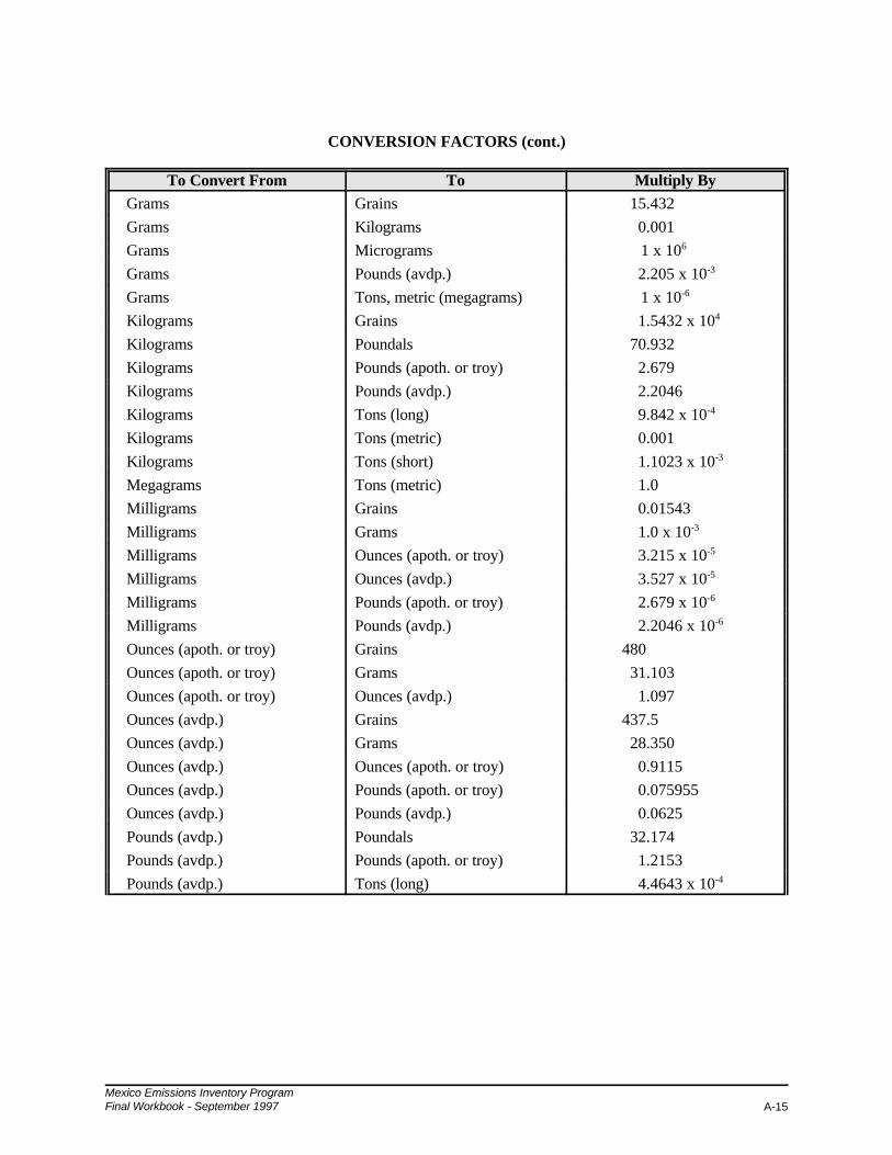
CONVERSION FACTORS (cont.)
To Convert From To Multiply By
Mexico Emissions Inventory ProgramFinal Workbook - September 1997 A-15
Grams Grains 15.432
Grams Kilograms 0.001
Grams Micrograms 1 x 10⁶
Grams Pounds (avdp.) 2.205 x 10⁻³
Grams Tons, metric (megagrams) 1 x 10⁻⁶
Kilograms Grains 1.5432 x 10⁴
Kilograms Poundals 70.932
Kilograms Pounds (apoth. or troy) 2.679
Kilograms Pounds (avdp.) 2.2046
Kilograms Tons (long) 9.842 x 10⁻⁴
Kilograms Tons (metric) 0.001
Kilograms Tons (short) 1.1023 x 10⁻³
Megagrams Tons (metric) 1.0
Milligrams Grains 0.01543
Milligrams Grams 1.0 x 10⁻³
Milligrams Ounces (apoth. or troy) 3.215 x 10⁻⁵
Milligrams Ounces (avdp.) 3.527 x 10⁻⁵
Milligrams Pounds (apoth. or troy) 2.679 x 10⁻⁶
Milligrams Pounds (avdp.) 2.2046 x 10⁻⁶
Ounces (apoth. or troy) Grains 480
Ounces (apoth. or troy) Grams 31.103
Ounces (apoth. or troy) Ounces (avdp.) 1.097
Ounces (avdp.) Grains 437.5
Ounces (avdp.) Grams 28.350
Ounces (avdp.) Ounces (apoth. or troy) 0.9115
Ounces (avdp.) Pounds (apoth. or troy) 0.075955
Ounces (avdp.) Pounds (avdp.) 0.0625
Pounds (avdp.) Poundals 32.174
Pounds (avdp.) Pounds (apoth. or troy) 1.2153
Pounds (avdp.) Tons (long) 4.4643 x 10⁻⁴

CONVERSION FACTORS (cont.)
To Convert From To Multiply By
Mexico Emissions Inventory ProgramFinal Workbook - September 1997A-16
Pounds (avdp.) Tons (metric) 4.5359 x 10⁻⁴
Pounds (avdp.) Tons (short) 5.0 x 10⁻⁴
Pounds (avdp.) Grains 7000
Pounds (avdp.) Grams 453.59
Pounds (avdp.) Ounces (apoth. or troy) 14.583
Pounds (avdp.) Ounces (avdp.) 16
Tons (long) Kilograms 1.016 x 10³
Tons (long) Pounds (apoth. or troy) 2.722 x 10³
Tons (long) Pounds (avdp.) 2.240 x 10³
Tons (long) Tons (metric) 1.016
Tons (long) Tons (short) 1.12
Tons (metric) Grams 1.0 x 10⁶
Tons (metric) Megagrams 1.0
Tons (metric) Pounds (apoth. or troy) 2.6792 x 10³
Tons (metric) Pounds (avdp.) 2.2046 x 10³
Tons (metric) Tons (long) 0.9842
Tons (metric) Tons (short) 1.1023
Tons (short) Kilograms 907.18
Tons (short) Pounds (apoth. or troy) 2.4301 x 10³
Tons (short) Pounds (avdp.) 2000
Tons (short) Tons (long) 0.8929
Tons (short) Tons (metric) 0.9072
Pressure
Atmospheres cm of H2O (4EC) 1.033 x 10³
Atmospheres Ft of H2O (39.2EF) 33.8995
Atmospheres In. of Hg (32EF) 29.9213
Atmospheres kg/sq cm 1.033
Atmospheres mm of Hg (0EC) 760
Atmospheres Pounds/sq inch 14.696
Inches of Hg (60EF) Atmospheres 0.03333

CONVERSION FACTORS (cont.)
To Convert From To Multiply By
Mexico Emissions Inventory ProgramFinal Workbook - September 1997 A-17
Inches of Hg (60EF) Grams/sq cm 34.434
Inches of Hg (60EF) mm of Hg (60EF) 25.4
Inches of Hg (60EF) Pounds/sq ft 70.527
Inches of H2O (4EC) Atmospheres 2.458 x 10⁻³
Inches of H2O (4EC) In. of Hg (32EF) 0.07355
Inches of H2O (4EC) kg/sq meter 25.399
Inches of H2O (4EC) Pounds/sq ft 5.2022
Inches of H2O (4EC) Pounds/sq inch 0.036126
Kilograms/sq cm Atmospheres 0.96784
Kilograms/sq cm cm of Hg (0EC) 73.556
Kilograms/sq cm Ft of H2O (39.2EF) 32.809
Kilograms/sq cm In. of Hg (32EF) 28.959
Kilograms/sq cm Pounds/sq inch 14.223
Millimeters of Hg (0EC) Atmospheres 1.3158 x 10⁻³
Millimeters of Hg (0EC) Grams/sq cm 1.3595
Millimeters of Hg (0EC) Pounds/sq inch 0.019337
Pounds/sq inch Atmospheres 0.06805
Pounds/sq inch cm of Hg (0EC) 5.1715
Pounds/sq inch cm of H2O (4EC) 70.309
Pounds/sq inch In. of Hg (32EF) 2.036
Pounds/sq inch In. of H2O (39.2EF) 27.681
Pounds/sq inch kg/sq cm 0.07031
Pounds/sq inch mm of Hg (0EC) 51.715
Velocity
Centimeters/sec Feet/min 1.9685
Centimeters/sec Feet/sec 0.0328
Centimeters/sec Kilometers/hr 0.036
Centimeters/sec Meters/min 0.6
Centimeters/sec Miles/hr 0.02237

CONVERSION FACTORS (cont.)
To Convert From To Multiply By
Mexico Emissions Inventory ProgramFinal Workbook - September 1997A-18
Feet/minute cm/sec 0.508
Feet/minute Kilometers/hr 0.01829
Feet/minute Meters/min 0.3048
Feet/minute Meters/sec 5.08 x 10⁻³
Feet/minute Miles/hr 0.01136
Feet/sec cm/sec 30.48
Feet/sec Kilometers/hr 1.0973
Feet/sec Meters/min 18.288
Feet/sec Miles/hr 0.6818
Kilometers/hr cm/sec 27.778
Kilometers/hr Feet/hr 3.2808 x 10³
Kilometers/hr Feet/min 54.681
Kilometers/hr Meters/sec 0.27778
Kilometers/hr Miles (statute)/hr 0.62137
Meters/min cm/sec 1.6667
Meters/min Feet/min 3.2808
Meters/min Feet/sec 0.05468
Meters/min Kilometers/hr 0.06
Miles/hr cm/sec 44.704
Miles/hr Feet/hr 5280
Miles/hr Feet/min 88
Miles/hr Feet/sec 1.4667
Miles/hr Kilometers/hr 1.6093
Miles/hr Meters/min 26.822
Volume
Barrels (petroleum, U. S.) Cu feet 5.6146
Barrels (petroleum, U. S.) Gallons (U. S.) 42
Barrels (petroleum, U. S.) Liters 158.98
Barrels (U. S., liq.) Cu feet 4.2109
Barrels (U. S., liq.) Cu inches 7.2765 x 10³

CONVERSION FACTORS (cont.)
To Convert From To Multiply By
Mexico Emissions Inventory ProgramFinal Workbook - September 1997 A-19
Barrels (U. S., liq.) Cu meters 0.1192
Barrels (U. S., liq.) Gallons (U. S., liq.) 31.5
Barrels (U. S., liq.) Liters 119.24
Cubic centimeters Cu feet 3.5315 x 10⁻⁵
Cubic centimeters Cu inches 0.06102
Cubic centimeters Cu meters 1.0 x 10⁻⁶
Cubic centimeters Cu yards 1.308 x 10⁻⁶
Cubic centimeters Gallons (U. S., liq.) 2.642 x 10⁻⁴
Cubic centimeters Quarts (U. S., liq.) 1.0567 x 10⁻³
Cubic feet Cu centimeters 2.8317 x 10⁴
Cubic feet Cu meters 0.028317
Cubic feet Gallons (U. S., liq.) 7.4805
Cubic feet Liters 28.317
Cubic inches Cu cm 16.387
Cubic inches Cu feet 5.787 x 10⁻⁴
Cubic inches Cu meters 1.6387 x 10⁻⁵
Cubic inches Cu yards 2.1433 x 10⁻⁵
Cubic inches Gallons (U. S., liq.) 4.329 x 10⁻³
Cubic inches Liters 0.01639
Cubic inches Quarts (U. S., liq.) 0.01732
Cubic meters Barrels (U. S., liq.) 8.3864
Cubic meters Cu cm 1.0 x 10⁶
Cubic meters Cu feet 35.315
Cubic meters Cu inches 6.1024 x 10⁴
Cubic meters Cu yards 1.308
Cubic meters Gallons (U. S., liq.) 264.17
Cubic meters Liters 1000
Cubic yards Bushels (Brit.) 21.022
Cubic yards Bushels (U. S.) 21.696
Cubic yards Cu cm 7.6455 x 10⁵

CONVERSION FACTORS (cont.)
To Convert From To Multiply By
Mexico Emissions Inventory ProgramFinal Workbook - September 1997A-20
Cubic yards Cu feet 27
Cubic yards Cu inches 4.6656 x 10⁴
Cubic yards Cu meters 0.76455
Cubic yards Gallons 168.18
Cubic yards Gallons 173.57
Cubic yards Gallons 201.97
Cubic yards Liters 764.55
Cubic yards Quarts 672.71
Cubic yards Quarts 694.28
Cubic yards Quarts 807.90
Gallons (U. S., liq.) Barrels (U. S., liq.) 0.03175
Gallons (U. S., liq.) Barrels (petroleum, U. S.) 0.02381
Gallons (U. S., liq.) Bushels (U. S.) 0.10742
Gallons (U. S., liq.) Cu centimeters 3.7854 x 10³
Gallons (U. S., liq.) Cu feet 0.13368
Gallons (U. S., liq.) Cu inches 231
Gallons (U. S., liq.) Cu meters 3.7854 x 10⁻³
Gallons (U. S., liq.) Cu yards 4.951 x 10⁻³
Gallons (U. S., liq.) Gallons (wine) 1.0
Gallons (U. S., liq.) Liters 3.7854
Gallons (U. S., liq.) Ounces (U. S., fluid) 128.0
Gallons (U. S., liq.) Pints (U. S., liq.) 8.0
Gallons (U. S., liq.) Quarts (U. S., liq.) 4.0
Liters Cu centimeters 1000
Liters Cu feet 0.035315
Liters Cu inches 61.024
Liters Cu meters 0.001
Liters Gallons (U. S., liq.) 0.2642
Liters Ounces (U. S., fluid) 33.814

CONVERSION FACTORS (cont.)
To Convert From To Multiply By
Mexico Emissions Inventory ProgramFinal Workbook - September 1997 A-21
Volumetric Rate
Cu ft/min Cu cm/sec 471.95
Cu ft/min Cu ft /hr 60. 0
Cu ft/min Gal (U. S.)/min 7.4805
Cu ft/min Liters/sec 0.47193
Cu meters/min Gal (U. S.)/min 264.17
Cu meters/min Liters/min 999.97
Gallons (U. S.)/hr Cu ft/hr 0.13368
Gallons (U. S.)/hr Cu meters/min 6.309 x 10⁻⁵
Gallons (U. S.)/hr Cu yd/min 8.2519 x 10⁻⁵
Gallons (U. S.)/hr Liters/hr 3.7854
Liters/min Cu ft/min 0.0353
Liters/min Gal (U. S., liq.)/min 0.2642a Where appropriate, the conversion factors appearing in this table have been rounded to four to six
significant figures for ease in use. The accuracy of these numbers is considered suitable for use withemissions data; if a more accurate number is required, tables containing exact factors should beconsulted.

Mexico Emissions Inventory ProgramFinal Workbook - September 1997A-22
CONVERSION FACTORS FOR COMMON AIR POLLUTION MEASUREMENTS
AIRBORNE PARTICULATE MATTER
To Convert From To Multiply By
Milligrams/cu m Grams/cu ft 283.2 x 10⁻⁶
Grams/cu m 0.001
Micrograms/cu m 1000.0
Micrograms/cu ft 28.32
Pounds/1000 cu ft 62.43 x 10⁻⁶
Grams/cu ft Milligrams/cu m 35.3145 x 10³
Grams/cu m 35.314
Micrograms/cu m 35.314 x 10⁶
Micrograms/cu ft 1.0 x 10⁶
Pounds/1000 cu ft 2.2046
Grams/cu m Milligrams/cu m 1000.0
Grams/cu ft 0.02832
Micrograms/cu m 1.0 x 10⁶
Micrograms/cu ft 28.317 x 10³
Pounds/1000 cu ft 0.06243
Micrograms/cu m Milligrams/cu m 0.001
Grams/cu ft 28.317 x 10⁻⁹
Grams/cu m 1.0 x 10⁻⁶
Micrograms/cu ft 0.02832
Pounds/1000 cu ft 62.43 x 10⁻⁹
Micrograms/cu ft Milligrams/cu m 35.314 x 10⁻³
Grams/cu ft 1.0 x 10⁻⁶
Grams/cu m 35.314 x 10⁻⁶
Micrograms/cu m 35.314
Pounds/1000 cu ft 2.2046 x 10⁻⁶
Pounds/1000 cu ft Milligrams/cu m 16.018 x 10³
Grams/cu ft 0.35314
Micrograms/cu m 16.018 x 10⁶
Grams/cu m 16.018
Micrograms/cu ft 353.14 x 10³
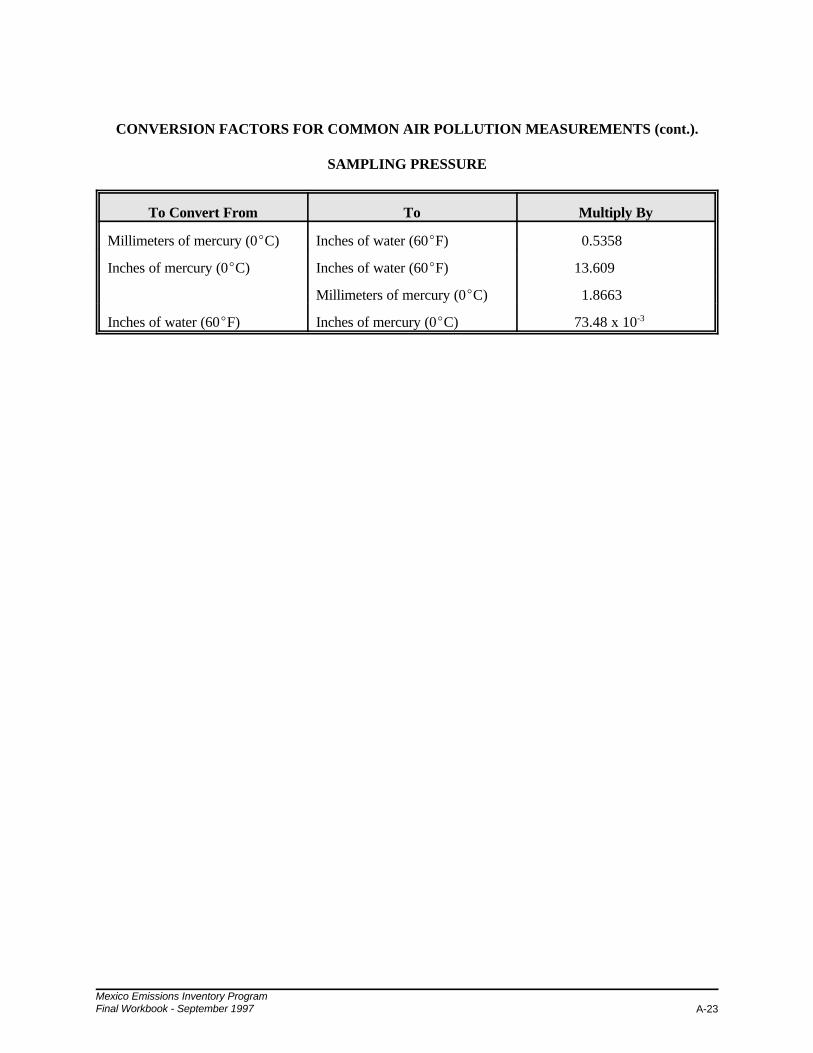
Mexico Emissions Inventory ProgramFinal Workbook - September 1997 A-23
CONVERSION FACTORS FOR COMMON AIR POLLUTION MEASUREMENTS (cont.).
SAMPLING PRESSURE
To Convert From To Multiply By
Millimeters of mercury (0EC) Inches of water (60EF) 0.5358
Inches of mercury (0EC) Inches of water (60EF) 13.609
Millimeters of mercury (0EC) 1.8663
Inches of water (60EF) Inches of mercury (0EC) 73.48 x 10⁻³
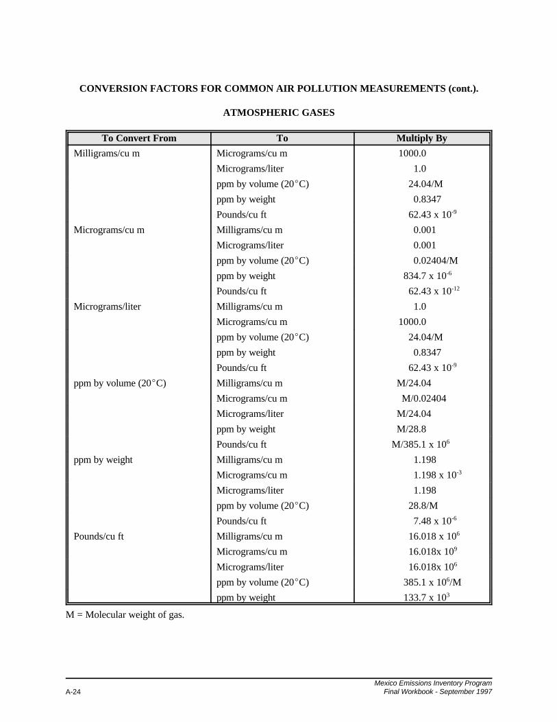
Mexico Emissions Inventory ProgramFinal Workbook - September 1997A-24
CONVERSION FACTORS FOR COMMON AIR POLLUTION MEASUREMENTS (cont.).
ATMOSPHERIC GASES
To Convert From To Multiply By
Milligrams/cu m Micrograms/cu m 1000.0
Micrograms/liter 1.0
ppm by volume (20EC) 24.04/M
ppm by weight 0.8347
Pounds/cu ft 62.43 x 10⁻⁹
Micrograms/cu m Milligrams/cu m 0.001
Micrograms/liter 0.001
ppm by volume (20EC) 0.02404/M
ppm by weight 834.7 x 10⁻⁶
Pounds/cu ft 62.43 x 10⁻¹²
Micrograms/liter Milligrams/cu m 1.0
Micrograms/cu m 1000.0
ppm by volume (20EC) 24.04/M
ppm by weight 0.8347
Pounds/cu ft 62.43 x 10⁻⁹
ppm by volume (20EC) Milligrams/cu m M/24.04
Micrograms/cu m M/0.02404
Micrograms/liter M/24.04
ppm by weight M/28.8
Pounds/cu ft M/385.1 x 106
ppm by weight Milligrams/cu m 1.198
Micrograms/cu m 1.198 x 10⁻³
Micrograms/liter 1.198
ppm by volume (20EC) 28.8/M
Pounds/cu ft 7.48 x 10⁻⁶
Pounds/cu ft Milligrams/cu m 16.018 x 10⁶
Micrograms/cu m 16.018x 10⁹
Micrograms/liter 16.018x 10⁶
ppm by volume (20EC) 385.1 x 10⁶/M
ppm by weight 133.7 x 10³
M = Molecular weight of gas.

Mexico Emissions Inventory ProgramFinal Workbook - September 1997 A-25
CONVERSION FACTORS FOR COMMON AIR POLLUTION MEASUREMENTS (cont.).
VELOCITY
To Convert From To Multiply ByMeters/sec Kilometers/hr 3.6
Feet/sec 3.281
Miles/hr 2.237
Kilometers/hr Meters/sec 0.2778
Feet/sec 0.9113
Miles/hr 0.6214
Feet/sec Meters/sec 0.3048
Kilometers/hr 1.09728
Miles/hr 0.6818
Miles/hr Meters/sec 0.4470
Kilometers/hr 1.6093
Feet/sec 1.4667
ATMOSPHERIC PRESSURE
To Convert From To Multiply ByAtmospheres Millimeters of mercury 760.0
Inches of mercury 29.92
Millibars 1013.2
Millimeters of mercury Atmospheres 1.316 x 10⁻³
Inches of mercury 39.37 x 10⁻³
Millibars 1.333
Inches of mercury Atmospheres 0.03333
Millimeters of mercury 25.4005
Millibars 33.35
Millibars Atmospheres 0.00987
Millimeters of mercury 0.75
Inches of mercury 0.30
VOLUME EMISSIONS
To Convert From To Multiply ByCubic m/min Cubic ft/min 35.314
Cubic ft/min Cubic m/min 0.0283
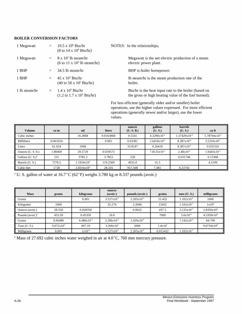
Mexico Emissions Inventory ProgramFinal Workbook - September 1997A-26
BOILER CONVERSION FACTORS
1 Megawatt = 10.5 x 10⁶ Btu/hr(8 to 14 x 106 Btu/hr)
NOTES: In the relationships,
1 Megawatt = 8 x 10³ lb steam/hr(6 to 11 x 103 lb steam/hr)
Megawatt is the net electric production of a steamelectric power plant.
1 BHP = 34.5 lb steam/hr BHP is boiler horsepower.
1 BHP = 45 x 103 Btu/hr(40 to 50 x 103 Btu/hr)
lb steam/hr is the steam production rate of theboiler.
1 lb steam/hr = 1.4 x 10³ Btu/hr(1.2 to 1.7 x 10³ Btu/hr)
Btu/hr is the heat input rate to the boiler (based onthe gross or high heating value of the fuel burned).
For less efficient (generally older and/or smaller) boileroperations, use the higher values expressed. For more efficientoperations (generally newer and/or larger), use the lowervalues.
Volume cu in ml litersounces
(U. S. fl.)gallons(U. S.)
barrels(U. S.) cu ft
Cubic inches 16.3868 0.0163868 0.5541 4.3290x10⁻³ 1.37429x10⁻⁴ 5.78704x10⁻⁴
Milliliters 0.061024 0.001 0.03381 2.6418x10⁻⁴ 8.387x10⁻⁶ 3.5316x10⁻⁵
Liters 61.024 1000 33.8147 0.26418 8.387x10⁻³ 0.035316
Ounces (U. S. fl.) 1.80469 29.5729 0.029573 7.8125x10⁻³ 2.48x10⁻⁴ 1.0443x10⁻³
Gallons (U. S.)a 231 3785.3 3.7853 128 0.031746 0.13368
Barrels (U. S.) 7276.5 1.1924x10⁵ 119.2369 4032.0 31.5 4.2109
Cubic feet 1728 2.8316x10⁴ 28.316 957.568 7.481 0.23743
a U. S. gallon of water at 16.7EC (62EF) weighs 3.780 kg or 8.337 pounds (avoir.)
Mass grams kilogramsounces(avoir.) pounds (avoir.) grains tons (U. S.) milligrams
Grams 0.001 3.527x10⁻² 2.205x10⁻³ 15.432 1.102x10⁻⁶ 1000
Kilograms 1000 35.274 2.2046 15432 1.102x10⁻³ 1x10⁶
Ounces (avoir.) 28.350 0.028350 0.0625 437.5 3.125x10⁻⁵ 2.8350x10⁴
Pounds (avoir.)a 453.59 0.45359 16.0 7000 5.0x10⁻⁴ 4.5359x10⁵
Grains 0.06480 6.480x10⁻⁵ 2.286x10⁻³ 1.429x10⁻⁴ 7.142x10⁻⁸ 64.799
Tons (U. S.) 9.072x10⁵ 907.19 3.200x10⁴ 2000 1.4x10⁷ 9.0718x10⁸
Milligrams 0.001 1x10⁻⁶ 3.527x10⁻⁵ 2.205x10⁻⁶ 0.015432 1.102x10⁻⁹
a Mass of 27.692 cubic inches water weighed in air at 4.0EC, 760 mm mercury pressure.

Mexico Emissions Inventory ProgramFinal Workbook - September 1997 A-27
Wor
k an
d E
nerg
yg
cal.
kg c
al.
ergs
joul
esB
tuft
lbkg
met
ers
L-A
tmH
P h
ours
ft p
ound
als
kWh
Wh
Gra
m c
alor
ies
(m
ean)
0.00
14.
186x
107
4.18
63.
9680
x10-3
3.08
740.
4268
50.
0413
111.
5593
x10-6
99.3
341.
1628
x10-6
1.16
28x1
0-3
Kilo
gram
cal
orie
s10
004.
186x
1010
4186
3.96
8030
87.4
426.
8541
.311
1.55
93x1
0-399
334
1.16
28x1
0-31.
1628
Erg
s2.
3889
x10-8
2.38
89x1
0-11
1x10
-79.
4805
x10-1
17.
3756
x10-8
1.01
97x1
0-89.
8689
x10-1
03.
7251
x10-1
42.
3730
x10-6
2.77
78x1
0-14
2.77
78x1
0-11
Joul
es0.
2388
92.
3889
x10-4
1x10
79.
4805
x10-4
0.73
756
0.10
197
9.86
89x1
0-33.
7251
x10-7
23.7
302.
7778
x10-7
2.77
78x1
0-4
Btu
(m
ean)
251.
980.
2519
81.
0548
x1010
1054
.877
7.98
107.
5610
.409
3.92
92x1
0-42.
5030
x104
2.93
0x10
-40.
2930
Foot
pou
nds
0.32
389
3.23
89x1
0-41.
3558
2x10
71.
3558
1.28
54x1
0-30.
1382
50.
0133
815.
0505
x10-7
32.1
743.
7662
x10-7
3.76
62x1
0-4
Kilo
gram
met
ers
2.34
272.
3427
x10-3
9.80
66x1
079.
8066
9.29
67x1
0-37.
2330
0.09
6781
3.65
29x1
0-623
2.71
2.72
41x1
0-62.
7241
x10-3
Lite
r at
mos
pher
es (
norm
al)
24.2
062.
4206
x10-2
1.01
33x1
0910
1.32
80.
0960
674
.735
10.3
333.
7745
x10-5
2404
.52.
8164
x10-5
2.81
64x1
0-2
Hor
sepo
wer
hou
rs6.
4130
x105
641.
302.
6845
x1013
2.68
45x1
0624
54.0
1.98
00x1
062.
7374
x105
2649
46.
3705
x107
0.74
5774
5.7
Foot
pou
ndal
s0.
0100
6710
.067
x10-6
4.21
402x
105
0.04
214
3.99
52x1
0-50.
0310
814.
2972
x10-3
4.15
58x1
0-41.
5697
x10-8
1.17
055x
10-8
1.17
055x
10-5
Kilo
wat
t hou
rs8.
6001
x105
860.
013.
6000
x1013
3.60
00x1
0634
13.0
2.65
52x1
063.
6709
x10-5
3.55
29x1
061.
3440
8.54
30x1
0710
00
Wat
t hou
rs86
0.01
0.86
001
3.60
00x1
01036
003.
4130
2655
.336
7.09
3.55
29x1
031.
3410
x10-3
8.54
30x1
010.
001
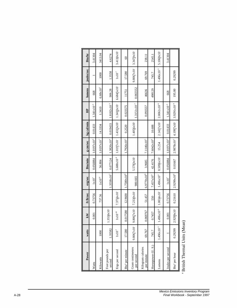
Mexico Emissions Inventory ProgramFinal Workbook - September 1997A-28
Pow
erw
atts
kWft
lb/s
ecer
g/se
cB
tu/m
ing
cm/s
eckg
cal
/min
HP
lum
ens
joul
es/s
ecB
tu/h
r
Wat
ts0.
001
0.73
756
1x10
70.
0568
841.
0197
x10
40.
0143
31.
341x
10-3
668
13.
4130
4
Kilo
wat
ts10
0073
7.56
1x10
1056
.884
1.01
97x1
07
14.3
334
1.34
106.
68x1
0510
0034
13.0
4
Foot
pou
nds
per
s
econ
d1.
3558
21.
3558
x10
-3
1.35
58x1
07
0.07
7124
1.38
26x1
04
0.01
9433
1.81
82x1
0-3
906.
281.
3558
4.62
74
Erg
s pe
r se
cond
1x10
-71x
10-1
07.
3756
x10
-8
5.68
8x10
-91.
0197
x10
-3
1.43
33x1
0-
91.
3410
x10
-10
6.68
45x1
0-
51x
10-7
3.41
30x1
0-
7
Btu
a per
min
ute
17.5
800.
0175
8012
.960
01.
7580
x10
81.
7926
x10
50.
2520
0.02
3575
1175
117
.580
60
Gra
m c
entim
eter
s p
er s
econ
d9.
8067
x10
-5
9.80
67x1
0-
87.
2330
x10
-5
980.
665
5.57
83x1
0-
61.
4056
x10
-6
1.31
51x1
0-7
0.06
5552
9.80
67x1
0-
53.
3470
x10
-4
Kilo
gram
cal
orie
s p
er m
inut
e69
.767
0.06
9767
51.4
576.
9770
x10
83.
9685
7.11
46x1
05
0.09
3557
4663
669
.769
238.
11
Hor
sepo
wer
(U
. S.)
745.
70.
7457
550
7.45
7x10
942
.417
67.
6042
x10
610
.688
4981
2974
5.7
2545
.1
Lum
ens
1.49
6x10
-31.
496x
10-6
1.00
34x1
0-
31.
496x
104
8.50
96x1
0-
515
.254
2.14
37x1
0-
52.
0061
x10
-61.
496x
10-3
5.10
69x1
0-
3
Joul
es p
er s
econ
d1
0.00
10.
7375
61x
107
0.05
6884
1.01
97x1
04
0.01
433
1.34
1x10
-366
83.
4130
4
Btu
a per
hou
r0.
2929
92.
9299
x10
-4
0.21
610
2.92
99x1
06
0.01
667
2.98
78x1
03
4.19
97x1
0-
33.
9291
x10
-419
5.80
0.29
299
a Bri
tish
The
rmal
Uni
ts (
Mea
n)

Mexico Emissions Inventory ProgramFinal Workbook - September 1997 A-29
CONVERSION FACTORS FOR VARIOUS SUBSTANCESa
Type Of Substance Conversion FactorsFuel
Oil 1 bbl = 159 liters (42 gal)
Natural gas 1 therm = 100,000 Btu (approx.25000 kcal)
Gaseous Pollutants
O3 1 ppm, volume = 1960Fg/m3
NO2 1 ppm, volume = 1880Fg/m3
SO2 1 ppm, volume = 2610Fg/m3
H2S 1 ppm, volume = 1390 Fg/m3
CO 1 ppm, volume = 1.14 mg/m3
HC (as methane) 1 ppm, volume = 0.654 mg/m3
Agricultural products
Corn 1 bu = 25.4 kg = 56 lb
Milo 1 bu = 25.4 kg = 56 lb
Oats 1 bu = 14.5 kg = 32 lb
Barley 1 bu = 21.8 kg = 48 lb
Wheat 1 bu = 27.2 kg = 60 lb
Cotton 1 bale = 226 kg = 500 lb
Mineral products
Brick 1 brick = 2.95 kg = 6.5 lb
Cement 1 bbl = 170 kg = 375 lb
Cement 1 yd3 = 1130 kg = 2500 lb
Concrete 1 yd3 = 1820 kg = 4000 lb
Mobile sources, fuel efficiency
Motor vehicles 1.0 mi/gal = 0.426 km/liter
Waterborne vessels 1.0 gal/naut mi = 2.05 liters/km
Miscellaneous liquids
Beer 1 bbl = 31.5 gal
Paint 1 gal = 4.5 to 6.82 kg = 10 to 15 lb
Varnish 1 gal = 3.18 kg = 7 lb
Whiskey 1 bbl = 190 liters = 50.2 gal
Water 1 gal = 3.81 kg = 8.3 lba Many of the conversion factors in this table represent average values and approximations and some of the
values vary with temperature and pressure. These conversion factors should, however, be sufficientlyaccurate for general field use.
APPENDIX B
INDEX OF EXAMPLE PROBLEMS IN
MEXICO EMISSIONS INVENTORY MANUALS

Mexico Emissions Inventory ProgramFinal Workbook - September 1997 B-1
Example Problems in Mexico Emissions Inventory Program Manuals
Volume III - Basic Emission Estimating Techniques
Section 3.2 Source Sampling DataSection 3.3 CEM DataSection 4.2.2 Multivariate ModelSection 5.10 Survey ResultsSection 6.1 Process-Based Emission FactorsSection 6.2 Census-Based Emission FactorsSection 7.0 Material BalanceSection 8.0 ExtrapolationAppendix III-A Emissions Models (fugitive dust, landfills, storage tanks, petroleum products
loading, waste and wastewater)
Volume IV - Point Source Inventory Development
Section 3.1 Emission FactorsSection 3.2 Source Test DataSection 3.3 Material BalanceSection 4.1 Fuel AnalysisSection 5.1 Control EffectivenessSection 7.3 Error Estimation
Volume V - Area Source Inventory Development
Section 4.0 Stationary Source Fuel CombustionSection 5.0 Non-Road Mobile SourcesSection 6.0 Solvent UseSection 7.0 Petroleum Product Storage and TransportSection 8.0 Light Industrial/Commercial SourcesSection 9.0 AgricultureSection 10.0 Waste ManagementSection 11.0 Miscellaneous Area Sources
Volume VI - Motor Vehicle Inventory Development
Section 3.4.1 Effects of Temperature, Altitude, Fuel RVP, Oxygenated Fuels, Inspectionand Maintenance (I/M) Programs, and Anti-Tampering Programs (ATP)
Section 3.4.2 Effects of Vehicle Speed
Top Related