


Languages
Pages
Legal


INTERNATIONAL JOURNAL OF ADVANCED SCIENTIFIC RESEARCH AND TECHNOLOGY
ISSUE 2, VOLUME 3 (JUNE- 2012) ISSN: 2249-9954
Page 21
A Survey - Mathematical Morphology operations on
Images in MATLAB Suresha D
1, Dr. Ganesh V. Bhat
2
Asst. Professor, Dept. of CSE, Canara Engineering College Mangalore, Karnataka,
Phone No:09141854528, [email protected].
Professor & Head, Dept. of ECE, Canara Engineering College Mangalore, Karnataka,
Phone No: 08762115169, [email protected]
ABSTRACT
Mathematical morphology is a theory and technique for the analysis and processing
of geometrical structures, based on set theory, lattice theory, topology, and random
functions. Morphology has an ability to make close range photogrammetric technology
faster and to simplify a human work. Morphology directly relate to shape of the object in
the image, majorly applied on grey scale and binary images. In this paper a survey has
been made on various mathematical morphology operations on binary images and
implemented in MATLAB. MATLAB is the most popular software for image processing
and used by many researchers in the field of image processing as each data representation
in it is treated as a matrix and as we know each image is a matrix of pixels and MATLAB
has number of tools built into it so, image processing through MATLAB is efficient.
Key words: Dilation, Erosion, Opening, Closing, Hit or Miss, Skeletonization
Corresponding Author: Suresha D
1. Introduction
Morphology is the identification, analysis and description of the structure.
Mathematical morphology is most commonly applied to digital images, but it can be
employed as well on graphs, surface meshes, solids, and many other spatial structures.
Topological and geometrical continuous space concepts such as size, shape, convexity,
connectivity, and geodesic distance, were introduced by mathematical morphology on both
continuous and discrete spaces. Mathematical morphology[1] is also the foundation of
morphological image processing, which consists of a set of operators that transform images
according to the characterizations.
Mathematical Morphology was originally developed for binary images, and was later
extended to grayscale functions and images. Mathematical morphology gives an approach to
the processing of digital images which is based on shape [2] of the object in the image.
Mathematical morphological operations tend to simplify image data preserving their essential
shape characteristics and eliminating irrelevancies. As the identification[3] of objects, object
features, and assembly defects correlate directly with shape, it becomes apparent that the
natural processing approach to deal with the machine vision[4] recognition process.
2. Classification of B&W images:
The below description explains on binary and grey images formation from the given
color image for which morphological operations applied.
A. Binary Images:
A binary image[5] is a digital image that has only two possible values for each pixel.
Typically the two colors used for a binary image are black and white though any two colors
can be used. The color used for the objects in the image is the foreground color while the rest
of the image is the background color. Binary images are also called bi-level or two-level. This

INTERNATIONAL JOURNAL OF ADVANCED SCIENTIFIC RESEARCH AND TECHNOLOGY
ISSUE 2, VOLUME 3 (JUNE- 2012) ISSN: 2249-9954
Page 22
means that each pixel is stored as a single bit (0 or 1). The names black-and-white, B&W,
monochrome or monochromatic are often used for this concept, but may also designate any
images that have only one sample per pixel.
BW = im2bw(I, level)-----------------(i)
Above function converts the color image I to a binary image. The output image BW
replaces all pixels in the input image with luminance greater than level with the value 1
(white) and replaces all other pixels with the value 0 (black). Specify level in the range (0,1).
Example:
x1=imread('c:\pic\suresh.jpg');
x2= im2bw(x1,0.5);
subplot(1,2,1), imshow(x1)
subplot(1,2,2), imshow(x2)
output:
(a) (b)
Figure 1: (a) Original Image (b) Binary Image
B. Grey Scale Images:
A grayscale or greyscale digital image is an image in which the value of each pixel
carries intensity[6] information. Images of this sort, also known as black-and-white, are
composed exclusively of shades of gray, varying from black at the weakest intensity to white
at the strongest. Grayscale images are distinct from one-bit bi-tonal black-and-white images,
which in the context of computer imaging are images with only the two colors, black, and
white (also called bilevel or binary images). Grayscale images have many shades of gray in
between. Grayscale images are also called monochromatic, denoting the presence of only one
(mono) color (chrome). Grayscale images are often the result of measuring the intensity of
light at each pixel in a single band of the electromagnetic spectrum (e.g. infrared, visible
light, ultraviolet, etc.), and in such cases they are monochromatic proper when only a given
frequency is captured.
I = rgb2gray(RGB)-------------(ii)
Above function converts the truecolor image RGB to the grayscale intensity image I.
rgb2gray converts RGB images to grayscale by eliminating the hue and saturation
information while retaining the luminance.
newmap = rgb2gray(map) returns a grayscale colormap equivalent to map.
Example:
x1=imread('c:\pic\suresh.jpg');
x3=rgb2gray(x1);
subplot(1,2,1), imshow(x1)
subplot(1,2,2), imshow(x3)
INTERNATIONAL JOURNAL OF ADVANCED SCIENTIFIC RESEARCH AND TECHNOLOGY
ISSUE 2, VOLUME 3 (JUNE- 2012) ISSN: 2249-9954
Page 23
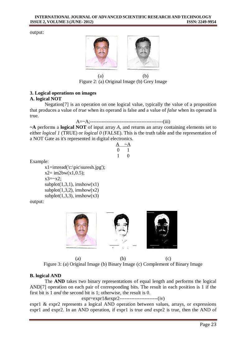
output:
(a) (b)
Figure 2: (a) Original Image (b) Grey Image
3. Logical operations on images
A. logical NOT
Negation[7] is an operation on one logical value, typically the value of a proposition
that produces a value of true when its operand is false and a value of false when its operand is
true.
A=~A;--------------------------------------------(iii)
~A performs a logical NOT of input array A, and returns an array containing elements set to
either logical 1 (TRUE) or logical 0 (FALSE). This is the truth table and the representation of
a NOT Gate as it's represented in digital electronics.
A ~A
0 1
1 0
Example:
x1=imread('c:\pic\suresh.jpg');
x2= im2bw(x1,0.5);
x3=~x2;
subplot(1,3,1), imshow(x1)
subplot(1,3,2), imshow(x2)
subplot(1,3,3), imshow(x3)
output:
(a) (b) (c)
Figure 3: (a) Original Image (b) Binary Image (c) Complement of Binary Image
B. logical AND
The AND takes two binary representations of equal length and performs the logical
AND[7] operation on each pair of corresponding bits. The result in each position is 1 if the
first bit is 1 and the second bit is 1; otherwise, the result is 0.
expr=expr1&expr2-----------------------(iv)
expr1 & expr2 represents a logical AND operation between values, arrays, or expressions
expr1 and expr2. In an AND operation, if expr1 is true and expr2 is true, then the AND of

INTERNATIONAL JOURNAL OF ADVANCED SCIENTIFIC RESEARCH AND TECHNOLOGY
ISSUE 2, VOLUME 3 (JUNE- 2012) ISSN: 2249-9954
Page 24
those inputs is true. If either expression is false, the result is false. Here is a pseudocode
example of AND:
IF (expr1: all required inputs were passed) AND ...
(expr2: all inputs are valid)
THEN (result: execute the function)
Example:
x1=imread('c:\pic\suresh.jpg');
x2= im2bw(x1,0.5);
x3=imread('c:\pic\suneetha.jpg');
x4=im2bw(x3,0.5);
x5=imresize(x4,size(x2));
x6=x2&x5;
subplot(3,2,1), imshow(x1)
subplot(3,2,2), imshow(x2)
subplot(3,2,3), imshow(x3)
subplot(3,2,4), imshow(x4)
subplot(3,2,5), imshow(x6)
Output:
Figure 4: (a) RGB Image1 (b) Binary Image of (a) (c) RGB Image2 (d) Binary Image of (c)
(e) Result of (b) and (d)
C. logical OR
A OR takes two bit patterns of equal length and performs the logical inclusive OR[7]
operation on each pair of corresponding bits. The result in each position is 1 if the first bit is 1
or the second bit is 1 or both bits are 1; otherwise, the result is 0. In this, we perform the
addition of two bits, i.e. 0 + 1 = 1, however 1 + 1 = 1.
expr=expr1 | expr2-----------------------(v)
expr1 | expr2 represents a logical OR operation between values, arrays, or expressions expr1
and expr2. In an OR operation, if expr1 is true or expr2 is true, then the OR of those inputs is
true. If both expressions are false, the result is false. Here is a pseudocode example of OR:
IF (expr1: S is a string) OR ...
(expr2: S is a cell array of strings)
THEN (result: parse string S)
a
b
c d
e

INTERNATIONAL JOURNAL OF ADVANCED SCIENTIFIC RESEARCH AND TECHNOLOGY
ISSUE 2, VOLUME 3 (JUNE- 2012) ISSN: 2249-9954
Page 25
Example:
x1=imread('c:\pic\suresh.jpg');
x2= im2bw(x1,0.5);
x3=imread('c:\pic\suneetha.jpg');
x4=im2bw(x3,0.5);
x5=imresize(x4,size(x2));
x6=x2|x5;
subplot(3,2,1), imshow(x1)
subplot(3,2,2), imshow(x2)
subplot(3,2,3), imshow(x3)
subplot(3,2,4), imshow(x4)
subplot(3,2,5), imshow(x6)
Output:
Figure 5: (a) RGB Image1 (b) Binary Image of (a) (c) RGB Image2 (d) Binary Image of (c)
(e) Result of (b) or (d)
4. Morphological Operations
Some of the basic morphological operations are
Dilation
Erosion
Opening
Closing
Hit or Miss
Skeletonization
A. Dilation:
Dilation is one of the basic operators in the area of mathematical morphology. It is
typically applied to binary images. The basic effect of the operator on a binary image is to
gradually enlarge[8] the boundaries of regions of foreground pixels (i.e. white pixels,
typically). Thus areas of foreground pixels grow in size while holes within those regions
become smaller. The dilation operator takes two pieces of data as inputs. The first is the
image which is to be dilated. The second is a (usually small) set of coordinate points known
as a structuring element. It is this structuring element that determines the precise effect of the
dilation on the input image.
Example:
x1=imread('c:\pic\suresh.jpg');
x2= im2bw(x1,0.5);
a b
c d
e
INTERNATIONAL JOURNAL OF ADVANCED SCIENTIFIC RESEARCH AND TECHNOLOGY
ISSUE 2, VOLUME 3 (JUNE- 2012) ISSN: 2249-9954
Page 26
x5=~x2;
x3=[0 0 1 0 0;0 1 1 1 0;1 1 1 1 1;0 1 1 1 0;0 0 1 0 0];
x4=imdilate(x5,x3);
x6=~x4;
subplot(3,2,1), imshow(x1)
subplot(3,2,2), imshow(x2)
subplot(3,2,3), imshow(x5)
subplot(3,2,4), imshow(x4)
subplot(3,2,5), imshow(x6)
Output:
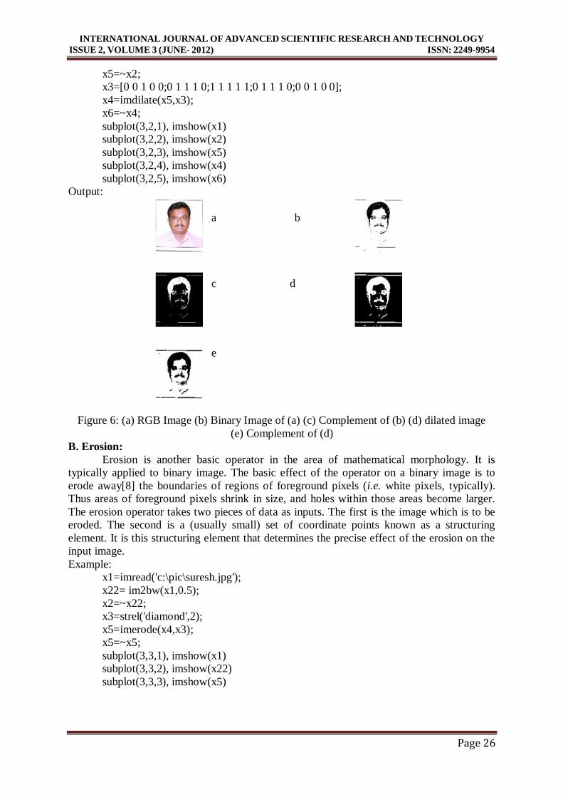
Figure 6: (a) RGB Image (b) Binary Image of (a) (c) Complement of (b) (d) dilated image
(e) Complement of (d)
B. Erosion:
Erosion is another basic operator in the area of mathematical morphology. It is
typically applied to binary image. The basic effect of the operator on a binary image is to
erode away[8] the boundaries of regions of foreground pixels (i.e. white pixels, typically).
Thus areas of foreground pixels shrink in size, and holes within those areas become larger.
The erosion operator takes two pieces of data as inputs. The first is the image which is to be
eroded. The second is a (usually small) set of coordinate points known as a structuring
element. It is this structuring element that determines the precise effect of the erosion on the
input image.
Example:
x1=imread('c:\pic\suresh.jpg');
x22= im2bw(x1,0.5);
x2=~x22;
x3=strel('diamond',2);
x5=imerode(x4,x3);
x5=~x5;
subplot(3,3,1), imshow(x1)
subplot(3,3,2), imshow(x22)
subplot(3,3,3), imshow(x5)
a b
c d
e

INTERNATIONAL JOURNAL OF ADVANCED SCIENTIFIC RESEARCH AND TECHNOLOGY
ISSUE 2, VOLUME 3 (JUNE- 2012) ISSN: 2249-9954
Page 27
(a) (b) (c)
Figure 7: (a) RGB Image (b) Binary Image (c) Erosion image
C. Opening:
The normal morphological opening is erosion followed by dilation[8]. The erosion
"shrinks" an image according to the shape of the structuring element, removing objects that
are smaller than the shape. Then the dilation step re grows the remaining objects by the same
shape.
Example:
x1=imread('C:\pic\suresh.jpg');
x3=im2bw(x1,0.5);
x5=strel('disk',3);
x6=imerode(x3,x5);
x5=strel('disk',3);
x7=imdilate(x6,x5);
subplot(1,4,1), imshow(x1)
subplot(1,4,1), imshow(x3)
subplot(1,4,2), imshow(x6)
subplot(1,4,3), imshow(x7)
Output:
Figure 8: (a) RGB Image (b) Binary Image (c) Erosion Image (d) dilated image of
erosion Image
D. Closing:
The normal morphological closing is a dilation followed by erosion[8]. The dilation
step "grows" the objects followed by the erosion which "shrinks" an image according to the
shape of the structuring element, removing objects that are smaller than the shape.
Example:
x1=imread('C:\pic\suresh.jpg');
x3=im2bw(x1,0.5);
a b
c d

INTERNATIONAL JOURNAL OF ADVANCED SCIENTIFIC RESEARCH AND TECHNOLOGY
ISSUE 2, VOLUME 3 (JUNE- 2012) ISSN: 2249-9954
Page 28
x5=strel('rectangle',[3 1]);
x7=imdilate(x3,x5);
x5=strel('rectangle',[1 3]);
x6=imerode(x7,x5);
subplot(2,2,1), imshow(x1)
subplot(2,2,2), imshow(x3)
subplot(2,2,3), imshow(x7)
subplot(2,2,4), imshow(x6)
Output:
Figure 9: (a) RGB Image (b) Binary Image (c) Dilation Image (d) Erosion image of
dilation Image
E. Hit or Miss Transformation
In mathematical morphology, hit-or-miss transform is an operation that detects a
given configuration[9] (or pattern) in a binary image, using the morphological erosion
operator and a pair of disjoint structuring elements. The result of the hit-or-miss transform is
the set of positions, where the first structuring element fits in the foreground of the input
image, and the second structuring element misses it completely.
Example:
x1=imread('C:\pic\suresh.jpg');
x2=im2bw(x1,0.5);
x3=~x2;
x4=[0 0 0;1 1 0;0 1 0];
x5=imerode(x2,x4);
x6=[0 1 0;0 0 1;1 0 0];
x7=imerode(x3,x6);
x8=x5&x7;
%x6=bwhitmiss(x3,x4,x5);
subplot(2,3,1), imshow(x1)
subplot(2,3,2), imshow(x2)
subplot(2,3,3), imshow(x3)
subplot(2,3,4), imshow(x5)
subplot(2,3,5), imshow(x7)
subplot(2,3,6), imshow(x8)
a b
c d

INTERNATIONAL JOURNAL OF ADVANCED SCIENTIFIC RESEARCH AND TECHNOLOGY
ISSUE 2, VOLUME 3 (JUNE- 2012) ISSN: 2249-9954
Page 29
Output:
Figure 9: (a) RGB Image (b) Binary Image (c) Complemented Image (d) Erosion image (b)
(e) Erosion Image of (c) (f) And image of (d)(e)
F. Skeletonization:
Skeleton (or topological skeleton) of a shape is a thin version of that shape that is
equidistant[10] to its boundaries. The skeleton usually emphasizes geometrical and
topological properties of the shape, such as its connectivity, topology, length, direction, and
width. Together with the distance of its points to the shape boundary, the skeleton can also
serve as a representation of the shape (they contain all the information necessary to
reconstruct the shape). Skeleton is an important shape property and has a variety of
applications.
Example:
x1=imread('trial.jpg');
x2=im2bw(x1,0.5);
x3=bwmorph(x2,'skel');
subplot(1,3,1), imshow(x1)
subplot(1,3,2), imshow(x2)
subplot(1,3,3), imshow(x3)
(a) (b) (c)
Figure 10: (a) Input Image (b) Binary Image (c) Skeletonized Image
5. Applications of Morphology:
A. Extraction of bank check items
This method extract the user-entered information from bank check images based on a
layout-driven[11] item extraction method. The baselines of checks are detected and
eliminated by using gray-level mathematical morphology. A priori information about the
positions of data is integrated into a combination of top-down and bottom-up analyses of
a b c
d e f

INTERNATIONAL JOURNAL OF ADVANCED SCIENTIFIC RESEARCH AND TECHNOLOGY
ISSUE 2, VOLUME 3 (JUNE- 2012) ISSN: 2249-9954
Page 30
check images. The handwritten information is extracted by a local thresholding technique and
the information lost during baseline elimination is restored by mathematical morphology with
dynamic kernels[].
Figure 11: bank check items
B. Genuine Fingerprint Feature Extraction
Mathematical morphology is used to remove the superfluous[12] information for
genuine feature extraction and measure the feature extraction performance through sensitivity
and specificity.
(a) (b)
Figure 12: (a)Input Fingerprint (b)Enhanced Image
C. Image Noise Reduction Using Mathematical Morphology
Morphological image cleaning algorithm (MIC)[13] that preserves thin features while
removing noise. MIC is useful for grayscale images corrupted by dense, low-amplitude,
random or patterned noise. The morphological image-cleaning algorithm will segment into
features and noise, the residual image that is the difference between an original image and a
smoothed version. The features from the residual are added back to the smoothed image.
Ideally, this results in an image whose edges and other one dimensional features are as sharp
as the original yet has smooth regions between them.
(a) (b)
Figure 13: (a)Input Image (b)Enhanced Image
D. Detection of Defects in Fabric by Morphological Image Processing
In binary morphological image processing first obtain binary image of the fabric.
Segmenting the gray level pixel values of fabric image[14] into two gray level values are all
that is required to produce a binary image of fabric. Let, I(i, j) is the gray level pixel value at
point (i,j) of the input fabric image and F(i,j) is the gray level of point (i,j) of the output fabric
image. The binary image is obtained from the gray level image by converting the pixel value
to 1 (white pixel) if the value is greater than the preselected threshold value: otherwise the
pixel value is returned to 0 (black pixel).

INTERNATIONAL JOURNAL OF ADVANCED SCIENTIFIC RESEARCH AND TECHNOLOGY
ISSUE 2, VOLUME 3 (JUNE- 2012) ISSN: 2249-9954
Page 31
Figure 14: Defects in Fabric
Detection of defects by morphological operators is carried out for few test samples of
woven fabric. For example, knot, thick weft and missing weft are subjected to morphological
operations with a 3×3 structuring element. Since the fabric images are gray images, gray to
binary image conversion by thresholding is necessary for defect detection. The morphological
erosion and opening operations are applied on the thresholded images. A rectangular
structuring element of 3×3 pixel size is sufficient for extracting the defects such as knot from
the test fabric either by erosion of by opening operations. However, in case of detection of
thick weft by opening operation is not very efficient though the detection is better than
erosion operation. The detection of missing weft by erosion and opening operations needs
higher size structuring element. A 5×5 rectangular structuring element gaves better results
than using a 3×3 structuring element. This is because of the continuity of the defective yarn
throughout the length / breadth of the test fabric.
Conclusion
In this paper some basic operations of morphological concepts are implemented. The
morphological concepts are having powerful set of tools for extracting features of interest in
an image. A significant advantage in terms of implementation is the fact that dilation and
erosion are primitive operations of morphology.
References:
[1] Mathematical Morphology
http://reference.wolfram.com/mathematica/guide/MathematicalMorphology.html
[2] Rafel C Gonzalez and Richard E. Woods,” Digital Image Processing”, PHI 2nd Edition
2005, pp. 541-582.
[3] Rafel C Gonzalez and Richard E. Woods, Steven L. Eddins, ”Digital Image Processing
using MATLAB”, Pearson Education, 2006, pp. 348-391.
[4] Scott.E.Umbaugh, “Computer Vision and Image Processing”, Prentice Hall, 1997.
[5] Amin Khajeh Djahromi,” Binary Image Processing,
http://www-ee.uta.edu/Online/Devarajan/ee6358/ BinaryImage.pdf
[6] 2003 R. Fisher, S. Perkins, A. Walker and E. Wolfart., “Grayscale Images “
http://homepages.inf.ed.ac.uk/rbf/HIPR2/gryimage.htm
[7] Vidya Manian, Ramón Vásquez and Praveen Katiyar , “Texture Classification Using
Logical Operators”, IEEE transactions on image processing, vol. 9, no. 10, october 2000.
http://ieeexplore.ieee.org/stamp/stamp.jsp?arnumber=00869181
[8] Su Chen and Robert M. Haralick,, “Recursive Erosion, Dilation, Opening, and Closing
Transforms”, IEEE transactions on image processing, vol. 4, no. 3, march 1995.
http://ieeexplore.ieee.org/stamp/stamp.jsp?arnumber=00366481.

INTERNATIONAL JOURNAL OF ADVANCED SCIENTIFIC RESEARCH AND TECHNOLOGY
ISSUE 2, VOLUME 3 (JUNE- 2012) ISSN: 2249-9954
Page 32
[9] Hit-and-Miss Transform.
[http://dip.sun.ac.za/~mfmaritz/DIP/hitmiss.pdf]
[10] Frank Y. Shih, Christopher C. Pu, “ A skeletonization algorithm by maxima tracking on
Euclidean distance transform”, Elsevier, Pattern Recognition, Volume 28, Issue 3, March
1995, Pages 331–341
[11] Xiangyun Ye, Mohamed Cheriet, Ching Y. Suen , Ke Liu,”Extraction of bankcheck
items by mathematical morphology”, International Journal on Document Analysis and
Recognition, Springer-Verlag, 1999, 2: 53–66.
[12] Vikas Humbe , S. S. Gornale, , Ramesh Manza, K. V. Kale , Mathematical Morphology
Approach for Genuine Fingerprint Feature Extraction
http://www.cscjournals.org/csc/manuscript/Journals/IJCSS/Volume1/Issue2/IJCSS-15.pdf
[13] Richard Alan Peters,”A new algorithm for image noise reduction using mathematical
morphology , IEEE transactions on image processing. vol. 4. no. 5. may 1995.
http://ieeexplore.ieee.org/ielx4/83/8672/00382491.pdf?tp=&arnumber=382491&isnumber=8
672
[14] Asit K. Datta and Jayanta K. Chandra,” Detection of Defects in Fabric by Morphological
Image Processing”.
http://cdn.intechopen.com/pdfs/12247/InTech-
Detection_of_defects_in_fabric_by_morphological_image_processing.p
Top Related