


Languages
Pages
Legal


A Subjective Foundation of Objective
Probability∗
Luciano De Castro† and Nabil I. Al-Najjar‡
First draft: December 2008; This version: May 2009
Abstract
De Finetti’s concept of exchangeability provides a way to formal-ize the intuitive idea of similarity and its role as guide in decisionmaking. His classic representation theorem states that exchangeableexpected utility preferences can be expressed in terms of a subjec-tive beliefs on parameters. De Finetti’s representation is inextricablylinked to expected utility as it simultaneously identifies the parametersand Bayesian beliefs about them. This paper studies the implicationsof exchangeability assuming that preferences are monotone, transitiveand continuous, but otherwise incomplete and/or fail probabilistic so-phistication. The central tool in our analysis is a new subjective ergodictheorem which takes as primitive preferences, rather than probabili-ties (as in standard ergodic theory). Using this theorem, we identifythe i.i.d. parametrization as sufficient for all preferences in our class.A special case of the result is de Finetti’s classic representation. Wealso prove: (1) a novel derivation of subjective probabilities based onfrequencies; (2) a subjective sufficient statistic theorem; and that (3)differences between various decision making paradigms reduce to howthey deal with uncertainty about a common set of parameters.
∗We thank Carlos Moreira, Mallesh Pai, Pablo Schenone, Kyoungwon Seo, EranShmaya, Marcelo Viana.† Department of Economics, University of Illinois, Urbana-Champaign.
E-mail: <[email protected]>.Research page : https://netfiles.uiuc.edu/luciano/www/‡ Department of Managerial Economics and Decision Sciences, Kellogg School of Man-
agement, Northwestern University, Evanston IL 60208.E-mail: <[email protected]>.Research page : http://www.kellogg.northwestern.edu/faculty/alnajjar/htm/index.htm

Contents
1 Introduction 1
2 States, Preferences and Acts 6
3 Exchangeability, Frequencies, and Subjective Probability 103.1 Exchangeability . . . . . . . . . . . . . . . . . . . . . . . . . . 103.2 Subjective Ergodic Theorem . . . . . . . . . . . . . . . . . . . 123.3 Frequencies as Subjective Probabilities . . . . . . . . . . . . . 133.4 Subjective Probabilities as Frequencies . . . . . . . . . . . . . 143.5 Subjective Sufficient Statistic Theorem . . . . . . . . . . . . . 17
4 Exchangeability, Ambiguity, and Objective Probabilities 194.1 Parameter-based Acts and de Finetti’s Theorem . . . . . . . . 194.2 Objective Probabilities as an Inter-subjective Consensus . . . 204.3 Statistical Ambiguity . . . . . . . . . . . . . . . . . . . . . . . 214.4 Ambiguity: Incomplete Preferences . . . . . . . . . . . . . . . 234.5 Ambiguity: Malevolent Nature . . . . . . . . . . . . . . . . . . 24
5 Discussion 275.1 De Finetti’s View of Similarity as Basis for Probability Judge-
ment . . . . . . . . . . . . . . . . . . . . . . . . . . . . . . . . 275.2 A Subjectivist Interpretation of Classical Statistics . . . . . . 285.3 Learning and Predictions . . . . . . . . . . . . . . . . . . . . . 29
A Proofs 30A.1 Regularity . . . . . . . . . . . . . . . . . . . . . . . . . . . . . 30A.2 Proof of Theorem 1 . . . . . . . . . . . . . . . . . . . . . . . 32A.3 Proof of Theorem 2 . . . . . . . . . . . . . . . . . . . . . . . . 39A.4 Proof of Theorem 3 . . . . . . . . . . . . . . . . . . . . . . . . 40A.5 Proof of Theorem 4 . . . . . . . . . . . . . . . . . . . . . . . . 45A.6 Proof of Theorem 5 . . . . . . . . . . . . . . . . . . . . . . . . 46A.7 Remaining Proofs . . . . . . . . . . . . . . . . . . . . . . . . . 47
1 Introduction
Theories of decision making under uncertainty can be viewed as developing
parsimonious representations of the environment decision makers face. A
leading example is Savage’s subjective expected utility theory. This theory
introduces axioms that reduce the problem of ranking potentially complex
state-contingent acts to calculating their expected utility with respect to a
subjective probability.
A different approach, prevalent in statistics, is to think about inference
in terms of “objective parameters” that summarize what is relevant about
the states of the world. Parametrizations act as information-compression
schemes through which inference and decision making can be expressed on a
parsimonious space of parameters, rather than the original primitive states.1
De Finetti’s notion of exchangeability makes it possible to integrate the
subjective and parametric approaches into one elegant theory. Specifically,
suppose that an experimental scientist or an econometrician conducts (or
passively observes) a sequence of observations in some set S. Since learning
from data requires pooling information across experiments, the scientist’s or
the econometrician’s inferences are predicated on the assumption, implicit or
explicit, that the experiments are, in a sense, “similar.”
De Finetti makes the intuitive idea of similarity formal through his no-
tion of exchangeability. Roughly, a decision maker subjectively views a set
of experiments as exchangeable if he treats the indices interchangeably.2 Dif-
ferent experiments will usually yield different outcomes, each of which is the
result of a multitude of poorly understood factors. Nevertheless, the subjec-
tive judgment that the experiments are exchangeable amounts to subjectively
believing that they are governed by the same underlying stochastic structure.
De Finetti’s celebrated representation says that a probability distribution P
1Sims (1996) articulates the view that scientific modeling is a process of finding appro-priate data compression schemes via parametric representations.
2See de Finetti (1937). Somewhat more formally, exchangeability means that the de-cision maker ranks as indifferent an act f and the act f π that pays f after a finitepermutation of the coordinates π is applied. In particular, he considers an outcome s tobe just as likely to appear at time t as at time t′.
1

on Ω is exchangeable if and only if it has the parametric form:
P =
∫Θ
P θ dµ(θ). (1)
Here the parameter set Θ indexes the set of all i.i.d. distributions P θ with
marginal θ, and µ is a probability distribution on Θ. The decomposition (1)
says that a process is exchangeable if and only if it is i.i.d. with unknown
parameter (which we denote interchangeably as either θ or P θ).
This decomposition is a mathematical result about probability measures
which need not capture what is relevant for decision problems, like those en-
countered in statistical inference. To make the link between (1) and decision
making formal, let < be a preference relation on acts f : Ω → R. For every
such act f , define the corresponding parameter-based act, F : Θ→ R, by
F (θ) =
∫Ω
f dP θ
to express f in terms of the parameters, rather than the original states.
If < satisfies Savage’s axioms with exchangeable subjective belief P ,
de Finetti’s theorem immediately implies that a decision maker ranks two
acts f and g by first reducing them to the corresponding parameter-based
acts F and G, then ranking F and G according to their expected utilities∫ΘF dµ and
∫ΘGdµ, where µ is given by (1). De Finetti’s theorem thus in-
tegrates subjective beliefs and parametric representations by characterizing
exchangeable expected utility preferences as an expected utility preference
on parameter-based acts.
? ? ?
In de Finetti’s classic representation above, the identification of parame-
ters is inextricably tied to the expected utility criterion. On the other hand,
the concept of parameters as parsimonious representations of what is relevant
about a decision problem is meaningful and, indeed, widely used indepen-
dently of the expected utility criterion. De Finetti’s representation as it
stands holds little value to, say, classical statistics or the various approaches
to model ambiguity. Conceptually, we shall also argue that the subjective
belief in the similarity of experiments is of different nature than beliefs over
the parameter values.
2

This paper studies the implications of exchangeability for preferences that
are continuous, monotone and transitive, but may otherwise be incomplete
and/or fail probabilistic sophistication.3 These include, as special cases,
exchangeable versions of Bewley (1986)’s model of incomplete preferences,
Gilboa and Schmeidler (1989)’s multiple prior model, and classical statistics
procedures.
Our central result, Theorem 1, is a new subjective ergodic theorem. To
illustrate it in the stylized setting of coin tosses, let f1 denote the act that
pays 1 if the first coin turns Heads and 0 otherwise. At a state ω, define f ?(ω)
as the limiting average payoff of the sequence of acts fi, i = 1, 2, . . ., where fiis the analogous bet on the ith coin. Our subjective ergodic theorem states
that the act f ? is well-defined off a <-null set of states, and that fi ∼ f ?.
This roughly says that the decision maker perceives the uncertainty about
how the first coin might turn up as ‘equivalent’ to an uncertainty about the
limiting frequency of successive coin tosses.
To motivate the proof of this theorem, think of the set of finite permuta-
tions Π as a group of transformations on the state space Ω. Exchangeability
is precisely the assumption that indifference is preserved under group action:
for any event E and permutation π, the decision maker is indifferent between
betting on E and betting on the event π(E) consisting of all π-permutations
of elements of E. This plus our other conditions is sufficient to establish the
conclusion of the theorem, namely that any act is indifferent to its frequentist
limit.
As its name suggests, this theorem bears close analogy with the standard
ergodic theorem. However, the arguments used to prove that theorem are
inapplicable in our context since they fundamentally rely on the existence of
a probability measure on the state space. Our starting point, by contrast, is
a preference that may be incomplete and/or fail probabilistic sophistication.
In fact, our setting is completely deterministic; probabilities emerge as a
consequence exchangeability and some basic properties of the preference.
Theorem 2 provides a parametric representation of preferences. We show
that there is a partition Eθθ∈Θ of the state space with the following prop-
erties. Each Eθ admits a unique i.i.d. distribution P θ such that, off a null
3In the sense of Machina and Schmeidler (1992).
3

event, f ?(ω) =∫
Ωf dP θ(ω), where θ(ω) is the component of the partition to
which ω belongs (i.e., the unique θ such that ω ∈ Eθ). That is, the expected
utility of an act conditional on parameters is precisely the limiting frequency
of its payoff at a given state as this state is transformed by permutations. In
fact, f ? is nothing but the certainty-equivalent value of f given θ, and hence
constant on each Eθ.
Our third main result, Theorem 3, obtains a new frequentist character-
ization of subjective expected utility. We show that a decision maker with
ergodic preference must be a subjective expected utility maximizer with i.i.d.
beliefs whose marginal on any single experiment coincides with the empirical
frequencies. Ergodicity is a learnability condition, namely that the decision
maker believes that, off a <-null set, observing the state ω conveys nothing
useful in inferring the value of the parameter. Note that the crucial axioms in
Savage’s framework, such as completeness or the sure-thing-principle, are not
assumed. Rather, our theorem shows that a learnability condition implies
these normative properties.
Our final main result, Theorem 4, is a subjective sufficient statistic the-
orem. Given transitivity, we have f < g if and only if f ? < g?. Since each
state ω “belongs to” a unique parameter θ(ω), we may define a parameter-
based act directly on states as F(θ(ω)
)≡∫
Ωf dP θ(ω). Combining these
observations with the last theorem, we have:
f < g ⇐⇒ F(θ(·))
< G(θ(·)).
This says that the i.i.d. parametrization Θ is a sufficient statistic for the class
of exchangeable preferences, in the sense that in comparing any two acts
f and g, it is enough to compare the corresponding parameter contingent
acts F and G.
Collectively, our results show that, under exchangeability, one can narrow
the difference between various decision making paradigms to how they deal
with uncertainty about a common set of parameters. The classic de Finetti’s
theorem is the special case where the decision maker deals with this uncer-
tainty by introducing a prior on parameters and using the expected utility
criterion. But our framework covers more. First, Theorem 5, characterizes
the set of events in S treated as unambiguous by all decision makers, irrespec-
4
tive of their attitude towards ambiguity, as those whose empirical frequencies
do not depend on the state, off a <-null set. We then discuss consider specific
examples of decision criteria, including Bewley (1986)’s model of incomplete
preferences and Gilboa and Schmeidler (1989)’s MEU criterion. Decision
procedures in classical statistics and econometrics may be similarly incor-
porated. These models, while explicitly non-Bayesian, typically satisfy our
weak auxiliary assumptions and are thus covered by our theorems.
? ? ?
Our paper provides, among other things, a link between subjective pref-
erences and objective, frequentist probabilities. To put this contribution in
context, it is useful to outline the fundamental tenets underlying de Finetti’s
conception of subjective probability:4 (1) Subjectivity: probabilities are a de-
cision maker’s mental construct, revealed in his observed choices, to help him
make sense of his environment; (2) Exchangeability: an organizing principle
embodying the decision maker’s subjective similarity judgement, connecting
subjective beliefs with objective frequencies; (3) Bayesianism: the decision
maker has complete, coherent ranking of all acts.
Our model fully incorporates subjectivity and exchangeability. In par-
ticular, probabilities have no objective value, but exist only as cognitive
constructs in the mind of the decision maker. The third tenet of de Finetti’s
methodology, Bayesian beliefs, is both different in nature and, arguably, more
questionable. Our results indicate that exchangeability ensures the existence
of parameters P θ, and little else. De Finetti’s representation requires, in ad-
dition, that the decision maker has a prior on the set of parameters, a prior
about which exchangeability and frequencies have nothing to say. Thus, the
question whether a decision maker has such a prior is logically and con-
ceptually distinct from exchangeability and its core justification as a bridge
between subjective beliefs and objective information.
Our approach makes it possible to provide a new perspective on concepts
like “objective probabilities” and “true parameters” that are in common use
in statistics, economics, and decision theory. An intuitive idea is to define
objective probability in terms of frequencies. For example, the probability
4These appear, in one form or another, in most of his writings. Our exposition drawsfrom de Finetti (1937) and de Finetti (1989, originally published in 1931).
5

of Heads is the frequency with which Heads appear in a sequence of coin
tosses. This intuition quickly founders upon the observation that there are
uncountably many sequences where the limiting frequency of Heads does not
converge.5
Given our theorems, any decision maker with exchangeable preference
must believe that frequencies are well-defined off a subjectively null event.
For such decision maker, the definition of objective probabilities as frequen-
cies is meaningful. Needless to say, exchangeability, being a notion of simi-
larity of experiments is, of course, subjective since different decision makers
may hold different views about what is and isn’t similar.6
2 States, Preferences and Acts
We study decision problems defined on a state space Ω = S × S × · · · . We
assume that S is a Polish space, i.e., a complete separable metrizable space
of outcomes, endowed with the Borel σ-algebra S. Here, an outcome s may
represent something as simple as the result of tossing a coin, or as complex
as an observation of an elaborate scientific experiment.7 The state space
Ω reflects a sequence of such experiments indexed by “times” t = 1, 2, . . ..8
We shall denote a generic element of Ω by ω = (s1, s2, s3, ...) and assume
throughout the Borel σ-algebra over Ω, denoted Σ.
5And uncountably many sequences with limiting frequency of Heads equal to a, for anypredetermined value of a, and so on.
6 According to de Finetti (1989, p. 174), a proposition is objective if: “I always knowin what circumstances I must call such a proposition true, and in what others false. Mycalling it true or false implies nothing about my state of mind, signifies no judgement,has no conceptual value.” A subjective proposition, on the other hand, is one which “noexperience can prove [...] right, or wrong; nor, in general, could any conceivable criteriongive any objective sense to the distinction [...] between right and wrong.”
7We use the term ‘experiment’ loosely without any presumption of active experimen-tation on the part of the decision maker. Thus, an econometrician passively collectingevidence is observing the results of experiments in our sense.
8Formally, we study a static choice problem where the state space has a product struc-ture. Of course, the study of de Finetti-like representations is motivated by learning fromexperiments that repeat over time. We briefly discuss learning in Sections 5.3
6

An act is any bounded measurable function:
f : Ω→ R.
Let F denote the set of all acts. As usual, we identify a real number r with
the constant act that pays r regardless of the state.
Some of our results will refer to the set FFB ⊂ F of finitely-based acts
which depend on finitely many coordinates. Formally, an act f is finitely-
based if there is an integer N , depending on f , such that f is measurable
with respect to the algebra generated by events of the form ω : sn ∈ A for
n = 1, . . . , N and (measurable) A ⊂ S.
We will interpret acts as either real valued and assume risk neutrality, or
that they are directly measured in utils. One may justify the latter inter-
pretation by thinking of more primitive acts taking values in an unmodeled
space of consequences and von Neumann-Morgenstern utility mapping these
consequences to utils. This interpretations does entail a loss of generality
as it imposes joint restrictions on the space of consequences and the utility
function. Although it is possible to make explicit sets of conditions to justify
this interpretation, these conditions would distract us from the main points
of this paper.9
Our central object of study are preferences < on F . Throughout, we
assume that:
Assumption 1 (Preorder) < is reflexive and transitive.
Note that we do not require preferences to be complete, so preferences of
the type considered by Bewley (2002) or those implicit in classical statistical
procedures are allowed.
The next three assumptions impose conditions that can be easily derived
from well-known, more primitive properties of preferences. We choose not to
do so both for greater generality, and to focus on the role of exchangeability.
First, we introduce the usual monotonicity assumption (Savage’s P3):
9Ghirardato, Maccheroni, Marinacci, and Siniscalchi (2003) show that it is possible toconsider a convex combination of acts and values in utils as we assume here in a purelysubjective framework.
7

Assumption 2 (Monotonicity) If f(ω) ≥ g(ω) for all ω ∈ Ω, then f < g.
We further strengthen this condition to:
Assumption 3 (Strict Monotonicity for Consequences) For every x, y ∈R,
x > y =⇒ x y.
Next, we require that the preference does not reverse the ranking of acts
after the addition of a constant:
Assumption 4 (Additive Invariance) For any α ∈ R, f < g implies
f + α < g + α.
This assumption, which is satisfied in a broad class of preferences, can be
interpreted to mean that the decision maker does not take irrelevant sunk
cost into account.10 To violate this assumption would mean that a decision
maker who prefers f over g may, in a decision problem where he ‘first’ pays
an amount α then chooses between f and g, reverse his choice and select g.
Next we define an event E ⊂ Ω to be <-null if for all f , g and h ∈ F , we
have: [f(ω), if ω ∈ Eh(ω), if ω 6∈ E
]∼[g(ω), if ω ∈ Eh(ω), if ω 6∈ E
](2)
The next assumption introduces intuitive properties of null sets. First
some notation: for any event E, let 1E denote its indicator function.
Assumption 5 (Null sets) Either of the following two conditions is suffi-
cient to imply that an event E is null:
• 1E ∼ 0;
10 The term additive invariance was coined by Al-Najjar and Weinstein (2009). It canbe directly checked that this assumption is satisfied in, among others, Bewley (1986)’sincomplete preference model, Schmeidler (1989)’s Choquet expected utility, Gilboa andSchmeidler (1989)’s multiple prior preferences, Maccheroni, Marinacci, and Rustichini(2006)’s variational preferences, and Siniscalchi (2009)’s vector adjusted expected utilitypreferences.
8

• There exists α and β such that β > α and α1E < β1E.
This assumption is satisfied by all standard models of preferences studied
in the literature. The motivation for the first part is obvious. As for the
second part, suppose that β > α and α1E < β1E. Then, by monotonicity,
α1E ∼ β1E. Another use of monotonicity would lead to the conclusion that
(13) holds for f = β, g = α′, and h = 0 for all α′ ∈ [α, β]. This, however,
falls short of implying that E is null. The second item in the assumption
allows us to conclude that E is, in fact, null.
We finally introduce a continuity assumption on preferences. Given an
act f and a sequence of acts fn in F , we write fn → f to mean that the
event ω ∈ Ω : limn fn(ω) 6= f(ω) is <-null. We require:11 ,12
Assumption 6 (Continuity) Suppose that for a given pair of acts f, g ∈ Fthere are sequences fn, gn such that: (i) fn → f and gn → g; (ii)
|fn(ω)| ≤ b(ω) and |gn(ω)| ≤ b(ω), for all ω and some b ∈ F ; (iii) fn < gn.
Then f < g.
The conditions above are basic conditions we impose on all preferences
considered in this paper. Hence:
Definition 1 For the remainder of the paper, a preference < is any binary
relation on F , satisfying Assumptions 1-6.
An important special case is that of expected utility preferences, which
consist of preferences < that rank acts according to the expected utility
criterion:
f < g ⇐⇒∫
Ω
f dP ≥∫
Ω
g dP,
with respect to some subjective probability P .
11It is worth noting that, in the special case of expected utility preferences, this conditionis equivalent to countable additivity. See Lemma A.24 in the Appendix.
12Our continuity assumption is similar to Ghirardato, Maccheroni, Marinacci, and Sinis-calchi (2003)’s B3. They require that, if fn → f and gn → g pointwise and fn < gn foreach n, then f < g. Note that they do not require the sequences to be bounded by afunction b.
9

3 Exchangeability, Frequencies, and Subjec-
tive Probability
3.1 Exchangeability
The central property of preferences which we wish to study is exchangeability.
Let Π denote the set of finite permutations π : N→ N. Given an act f and
a permutation π : N → N, the act f π is defined as: f π(s1, s2, ...) =
f(sπ(1), sπ(2), ...).
As discussed in the Introduction, exchangeability reflects the decision
maker’s perception of similarity between experiments. For example, suppose
fi is the act that pays 1 if the outcome of experiment i is Heads and zero
otherwise. If π permutes the indices i, j, then fi π is just the act fj that
places a similar bet on the jth experiment. Exchangeability then says that
the decision maker is indifferent between betting on the ith and the jth
experiments.
More generally, a minimal requirement for exchangeability is that for
every act f ∈ F and permutation π ∈ Π,
f ∼ f π. (3)
Under expected utility, condition (3) is sufficient to establish the central
conclusion of de Finetti’s theorem, namely linking subjective probability and
frequencies. But de Finetti’s notion of exchangeability, being conceived for
the expected utility context, loses much of its force in our more general
setting. To recover the link between preferences and frequencies, we require:
Assumption 7 (Exchangeability) A preference < is exchangeable if for
every act f ∈ F and permutations π1, . . . , πn
f ∼ f π1 + · · ·+ f πnn
. (4)
This reduces to condition (3) when n = 1. Assuming expected utility, ex-
changeability can be derived from the weaker condition (3) with a simple
10

application of the independence axiom.13
As in de Finetti’s original conception (see Section 5.1), we view an ex-
changeability relationship as the decision maker’s subjective theory, or model,
of similarity. The need for similarity arises because the decision maker rec-
ognizes that the outcome of the coin toss is determined by a multitude of
poorly understood factors. This, after all, is why the coin sometimes comes
up Heads, and some other times Tails ! Exchangeability enables the decision
maker to pool information across experiments through the subjective judg-
ment that these poorly understood factors affect experiments symmetrically.
The minimal requirement f ∼ fπ goes some distance in formalizing our
intuition of the decision maker’s perception of similarity. But it is wholly
inadequate to capture the crucial insight in de Finetti’s classic theorem,
namely to identify parameters that we can meaningfully link to frequencies
and interpret as sufficient statistics for decision making. Our definition of
exchangeability (4) relates preferences to frequencies in a transparent way. In
the stylized setting of coin tosses, with f denoting the act that pays 1 if the
outcome of experiment 1 is Heads and zero otherwise, the term fπ1+···+fπnn
is
simply the frequency of Heads in the n tosses π1(1), . . . , πn(1). Exchangeabil-
ity simply requires that a (risk neutral) decision maker, who views experiment
1 as similar to each of the other experiments, should be indifferent between
betting on Heads in experiment 1 and betting on the frequency of Heads. It
is difficult to imagine how a meaningful link to frequencies can be established
without something like this condition.
Interpreting exchangeability as the decision maker’s subjective model of
similarity, it is natural to require that he be committed to whatever model he
has chosen. We formalize this commitment to a model by appealing to the
minimal version of the independence axiom implicit in (4). Independence is
applied only to the exchangeability indifferences, and only in so far as simple
averages are concerned. This is permissive enough to accommodate ambigu-
13The condition characterizing preferences that satisfy our central result, the subjectiveergodic theorem, is (11). We use (4) because it is stated in terms of permutations whichwe view as primitive, while (11) is stated in terms of shifts. In one of their theorems,Epstein and Seo (2008) use the condition that, for every f ∈ F , π ∈ Π, and α ∈ [0, 1],f ∼ αf + (1− α)fπ. Under our weak assumptions on preferences, this condition neitherimplies nor is implied by (4). See Section 4.5.
11
ity about the parameters. What we rule out is an incoherent decision maker
who views experiments as similar, yet he is not sure that they are. Such an
incoherent perception of what constitutes similar experiments is interesting
as a behavioral bias, but difficult to imagine as a basis for statistical and
econometric practice, or as a useful ingredient in economic models.
3.2 Subjective Ergodic Theorem
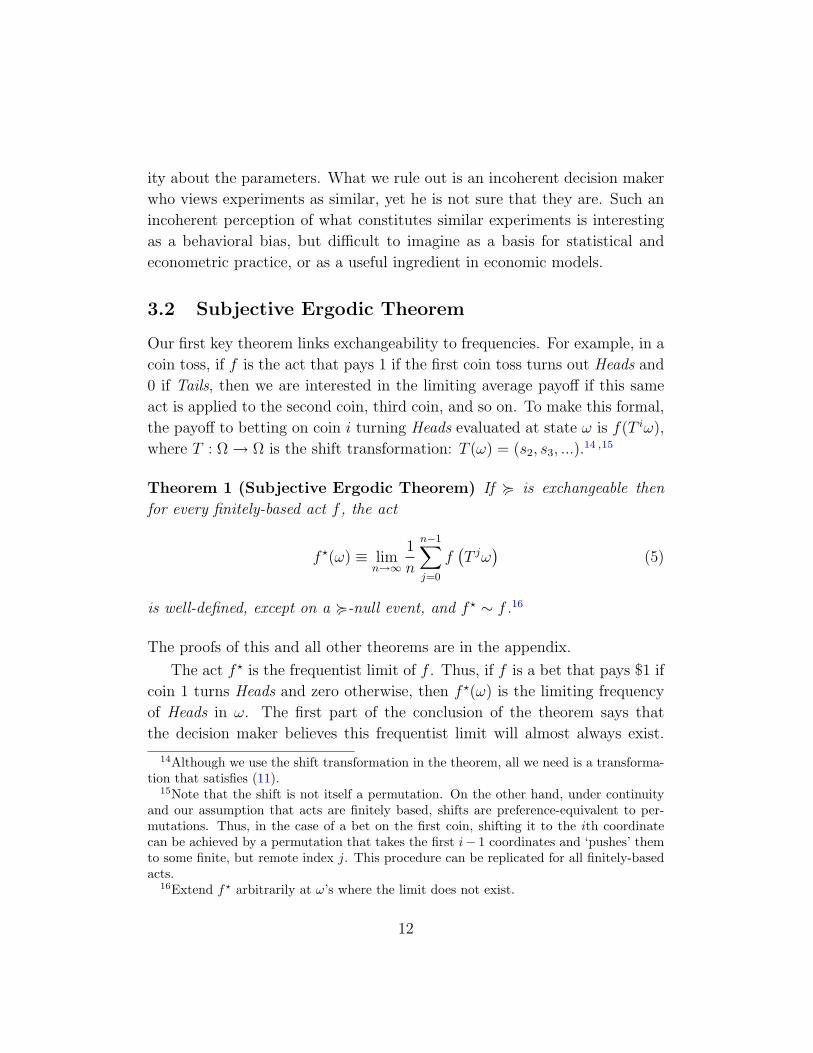
Our first key theorem links exchangeability to frequencies. For example, in a
coin toss, if f is the act that pays 1 if the first coin toss turns out Heads and
0 if Tails, then we are interested in the limiting average payoff if this same
act is applied to the second coin, third coin, and so on. To make this formal,
the payoff to betting on coin i turning Heads evaluated at state ω is f(T iω),
where T : Ω→ Ω is the shift transformation: T (ω) = (s2, s3, ...).14 ,15
Theorem 1 (Subjective Ergodic Theorem) If < is exchangeable then
for every finitely-based act f , the act
f ?(ω) ≡ limn→∞
1
n
n−1∑j=0
f(T jω
)(5)
is well-defined, except on a <-null event, and f ? ∼ f .16
The proofs of this and all other theorems are in the appendix.
The act f ? is the frequentist limit of f . Thus, if f is a bet that pays $1 if
coin 1 turns Heads and zero otherwise, then f ?(ω) is the limiting frequency
of Heads in ω. The first part of the conclusion of the theorem says that
the decision maker believes this frequentist limit will almost always exist.
14Although we use the shift transformation in the theorem, all we need is a transforma-tion that satisfies (11).
15Note that the shift is not itself a permutation. On the other hand, under continuityand our assumption that acts are finitely based, shifts are preference-equivalent to per-mutations. Thus, in the case of a bet on the first coin, shifting it to the ith coordinatecan be achieved by a permutation that takes the first i− 1 coordinates and ‘pushes’ themto some finite, but remote index j. This procedure can be replicated for all finitely-basedacts.
16Extend f? arbitrarily at ω’s where the limit does not exist.
12

Note that f ? does not vary across states with the same limiting frequency.
The second part of the theorem then says that frequencies are sufficient to
determine the preference: the decision maker is indifferent between f and its
reduction to an act f ? that collapses the variations of f over f ?-equivalent
states to a single value.
The standard ergodic theorem says that given a probability measure P
and a measure-preserving transformation, the limiting frequency converges
almost surely.17 While Theorem 1 is conceptually related to standard ergodic
theory, the differences are fundamental. In our case, the set of permutations
Π is a group of transformations, and exchangeability means that permuta-
tions are indifference-preserving. However, standard ergodic theorems start
with a measure on the state space, while our goal is to cover preferences
that are incomplete and/or fail probabilistic sophistication. So it is central
to our theorem that no probability measure is assumed. In fact, the only
primitive in Theorem 1 is the preference; the setting is otherwise completely
deterministic. Given this, a direct application of ergodic theory is stymied
at the start since there is no probability measure on the state space to begin
with.
We conclude by noting that, under an additional technical condition (As-
sumption 8), and building on the proofs of Theorems 1 and 3, we show in
Corollary 2 that the conclusion of Theorem 1 characterizes exchangeability.
3.3 Frequencies as Subjective Probabilities
Our next theorem provides a parametrization of exchangeable preferences.
First we introduce some standard definitions: given an event A ⊂ Ω and
permutation π ∈ Π, define πA to be the event consisting of all states
(sπ(1), sπ(2), ...) for some (s1, s2, ...) ∈ A. An event A is exchangeable if
A = πA for every permutation. A probability distribution P over Ω is
exchangeable if P (A) = P (πA) for every event A and permutation π. Let
Υ ⊂ ∆(Ω) denote the set of exchangeable distributions.
For any θ ∈ ∆(S), define θ∞ to be the product distribution of θ over Ω.
17For references on the standard ergodic theorem, see Billingsley (1995) and, for therelated idea of ergodic decomposition, Loh (2006).
13
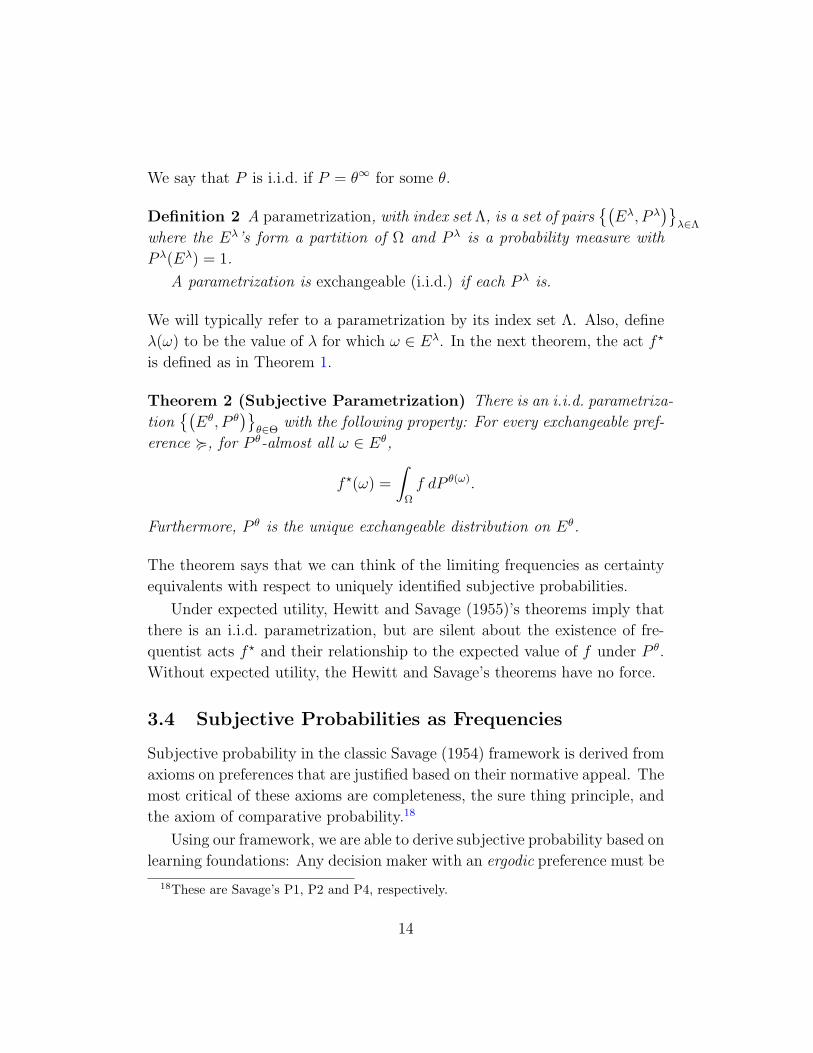
We say that P is i.i.d. if P = θ∞ for some θ.
Definition 2 A parametrization, with index set Λ, is a set of pairs(Eλ, P λ
)λ∈Λ
where the Eλ’s form a partition of Ω and P λ is a probability measure with
P λ(Eλ) = 1.
A parametrization is exchangeable (i.i.d.) if each P λ is.
We will typically refer to a parametrization by its index set Λ. Also, define
λ(ω) to be the value of λ for which ω ∈ Eλ. In the next theorem, the act f ?
is defined as in Theorem 1.
Theorem 2 (Subjective Parametrization) There is an i.i.d. parametriza-
tion(Eθ, P θ
)θ∈Θ
with the following property: For every exchangeable pref-
erence <, for P θ-almost all ω ∈ Eθ,
f ?(ω) =
∫Ω
f dP θ(ω).
Furthermore, P θ is the unique exchangeable distribution on Eθ.
The theorem says that we can think of the limiting frequencies as certainty
equivalents with respect to uniquely identified subjective probabilities.
Under expected utility, Hewitt and Savage (1955)’s theorems imply that
there is an i.i.d. parametrization, but are silent about the existence of fre-
quentist acts f ? and their relationship to the expected value of f under P θ.
Without expected utility, the Hewitt and Savage’s theorems have no force.
3.4 Subjective Probabilities as Frequencies
Subjective probability in the classic Savage (1954) framework is derived from
axioms on preferences that are justified based on their normative appeal. The
most critical of these axioms are completeness, the sure thing principle, and
the axiom of comparative probability.18
Using our framework, we are able to derive subjective probability based on
learning foundations: Any decision maker with an ergodic preference must be
18These are Savage’s P1, P2 and P4, respectively.
14

an expected utility maximizer, with subjective beliefs given by the empirical
frequencies.19 Ergodicity roughly means that the decision maker believes he
will not learn anything new by observing additional data. Thus, a learning
assumption is shown to imply the above mentioned Savage axioms.
First we need some formal definitions:
• E ⊂ Ω is <-trivial if either E or Ec is <-null;
• E is invariant if T (E) = E;
• < is ergodic if it is exchangeable and all invariant sets are <-trivial;
To appreciate the definition, consider a repeated coin toss and suppose
that a decision maker believes there are only two possible biases of the coin:
θ1 and θ2. Let Eθ1 and Eθ2 denote the sets of all sequences with limiting
frequencies θ1 and θ2, respectively. Then Eθ1 and Eθ2 are both invariant,
but not <-trivial. Here the lack of ergodicity corresponds to the existence of
events the uncertainty about which can be resolved via knowledge of the long
run frequencies. Given this, there is little we can say about how a decision
maker may evaluate the act f1 that pays 1 if the first coin turns Heads and
0 otherwise. The decision maker may have a Bayesian prior on θ1 and θ2,
ambiguous beliefs, or an incomplete preference. An ergodic preference, on
the other hand, is one for which such knowledge is of no value. Roughly, a
decision maker with an ergodic preference believes he has learned all that
can be learned about the uncertainty he faces.
For a subset A ⊂ S and state ω, the number 1?A(ω) is simply the frequency
of A in ω.20
Of course, for a given A and ω, the frequency may either fail to exist or
may depend on ω. The empirical distribution at ω is the set-function which
assigns to each A the value
ν(A, ω) ≡ 1?A(ω),
if this value exists, and is not defined otherwise.
19To our knowledge, the only other attempt to related subjective probabilities to fre-quencies appears in Hu (2008), who works in a von Neumann-Morgenstern setting anduses arguments quite distinct from ours.
20Here, we simplify notation by speaking of an event A ⊂ S to refer to A×S × · · · ∈ Σ.
15

Theorem 3 If < is ergodic, then:
• There is an event Ω′ with <-null complement, such that the empirical
distribution ν(·) = ν(·, ω) is a well-defined probability distribution on Sthat is constant in ω ∈ Ω′; and
• < is an expected utility preference with subjective probability P that is
i.i.d. with marginal ν.
A key difficulty in proving this theorem is ensuring that, unlike in Theorem
1, the set Ω′ does not depend on the act f .
It is useful to contrast this theorem with standard approach for deriving
subjective probability. In particular, we want to point out that our result
is not a generalization of the Savage-de Finetti framework, but a comple-
mentary derivation of subjective probability using very different principles.
Suppose we are given a < that satisfies our basic assumptions plus exchange-
ability.
• In the Savage-de Finetti approach, one begins by introducing norma-
tively motivated axioms on the preference, such as completeness and
the sure thing principle. From these axioms one uses standard methods
to derive a subjective expected utility representation. Since the sub-
jective probability thus derived is necessarily exchangeable, one may
use standard tools from probability theory (e.g., the ergodic theorem
or the law of large numbers) to derive results about the properties of
summary statistics like the empirical frequencies.
• Our theorem takes a completely different route: we steer clear from any
additional normative axiomatic assumption, and focus instead on what
the decision maker believes he can learn from observations (ergodicity).
We then use the subjective ergodic theorem and other results to derive
properties of empirical frequencies. From these properties we derive
an empirical measure and show that the decision maker must have
a subjective expected utility preference with subjective belief equal to
this measure. This in turn implies that the preference must be complete
and satisfies the sure thing principle.
16
We conclude by noting that the theorem can be applied under a weakening
of the assumption of ergodicity. Call a preference Σ′-ergodic if it is ergodic
with respect (Ω,Σ′), where Σ′ is a sub-σ-algebra of Σ. That is, we require:
• < is exchangeable and all invariant sets in Σ′ are <-trivial;
Then, with little change in the proof, we can conclude that < is an expected
utility preference over acts that are Σ′-measurable.
3.5 Subjective Sufficient Statistic Theorem
What makes a parametrization useful is that it captures all that is relevant
for the decision maker’s preference. This is closely related to the concept
of sufficiency in mathematical statistics. Recall that a measurable function
τ : Ω→ A, where A is an abstract measurable space, is a sufficient statistic
for a family of probability distributions P if the conditional distributions
P (· | τ) do not depend on P .21 Roughly, τ is sufficient if it captures all the
relevant information contained in a state ω: given knowledge that τ = τ , no
further information about ω is useful in drawing an inference about P .
In generalizing this intuition to preferences in a subjective framework,
two difficulties arise: First, since distributions in the statistics literature are
objective, sufficiency notions expressed in terms of objective probabilities
need not capture what is relevant for preferences. Second, sufficiency in the
statistics literature is inherently tied to probabilities, making it inapplicable
to preferences that may fail to be complete or probabilistically sophisticated.
To make the idea of sufficiency for preferences formal, given a parametriza-
tion Λ, define FΛ ⊂ F to be the set of acts measurable with respect to
Eλλ∈Λ.22 Define the mapping
ΦΛ : FFB → FΛ by ΦΛ(f)(ω) =
∫Ω
f dP λ(ω). (6)
We extend the notion of sufficiency to a subjective setting by defining:
21We are abstracting from measure theoretic issues regarding the definition of condi-tional probabilities for expository simplicity. See, for instance, Billingsley (1995).
22Formally, the sub-σ-algebra of Σ generated by the Eλ’s.
17

Definition 3 A parametrization Λ is sufficient for a set of preference rela-
tions E if for each <∈ E and finitely-based acts f and g
f < g ⇐⇒ ΦΛ(f) < ΦΛ(g). (7)
Thus, a parameterization is sufficient if the restriction of a preference to the
subset of acts FΛ is sufficient to determine the entire preference, simultane-
ously for all preferences in the class E .
Two things should be noted about the definition. First, the use of the
expected utility criterion implicit in the definition of ΦΛ defines what we mean
by a “parameter:” once the parameter is known, any remaining uncertainty
must be treated as risk. Without this criterion, sufficiency loses its meaning
as a device for compressing information. Second, subjective sufficiency, like
its counterpart in statistics, is a property of a class of preferences. It makes
little sense to talk about sufficiency for a single preference. For example, if
< is an expected utility preference with subjective belief P , then the trivial
parametrization (Ω, P ) is “sufficient” for <, trivially.
To establish the next theorem, we need an additional assumption of
mainly technical nature:
Assumption 8 For every <-non-null event E there is an i.i.d. distribution
P such that P (E) > 0.
If we think of a preference < as an aggregator of parameter-contingent pref-
erences, then the assumption says that < cannot be so badly behaved as to
treat as non-null an event that is conditionally null at each parameter.
Theorem 4 (Subjective Sufficient Statistic) The parametrization Θ in
Theorem 2 is sufficient for the set of exchangeable preferences satisfying As-
sumption 8.
18

4 Exchangeability, Ambiguity, and Objective
Probabilities
4.1 Parameter-based Acts and de Finetti’s Theorem
Given an act f ∈ F , its parameter-based reduction is the act:
F : Θ→ R where F (θ) =
∫Ω
f dP θ.
Conversely, for any act F : Θ→ R there corresponds an equivalence class of
state-based acts whose reduction is F . Here, F expresses the state-based act
f in terms of the parameters, and is essentially the same as ΦΘ(f) except that
we write it directly in terms of the parameters θ, rather than the primitive
states ω.
We are now in a position to state de Finetti’s classic result. By a belief on
a parametrization Λ we mean a probability distribution on Ω endowed with
the sub-σ-algebra of Σ generated by Eλλ∈Λ.
de Finetti’s Theorem: An expected utility preference < is exchangeable if
and only if there is a belief µ on Θ such that:
f < g ⇐⇒∫
Θ
F dµ ≥∫
Θ
Gdµ.
De Finetti’s theorem says that:
1. Θ is sufficient for the class of exchangeable expected utility preferences;
2. the decision maker resolves uncertainty about the parameters using the
expected utility criterion.
Our theorems show a stronger version of the first statement and entirely
drop the second: on the one hand, Θ is sufficient for all exchangeable pref-
erences, whether or not they have expected utility representation. On the
other hand, we allow preferences where decision makers need not reduce un-
certainty about parameters to risk.
19
We conclude by noting that the relationship between de Finetti’s theorem
and sufficient statistics has been discussed in the literature in the context
of expected utility preferences. See, for instance, Diaconis and Freedman
(1984), Lauritzen (1984), and Diaconis (1992). The general formulation we
have here is new.
4.2 Objective Probabilities as an Inter-subjective Con-sensus
An important application of our results is: To what extent would subjectivist
decision makers’ beliefs (dis-) agree? In particular, are there aspects of be-
liefs that all subjectivists agree on? In general, little can be said in this
regard. However, under exchangeability and Assumption 8, we can show
that preferences cannot contradict a Bayesian consensus.
Recall that Υ is the set of all exchangeable probability distributions. In
what follows, by an exchangeable Bayesian we shall mean an expected utility
decision maker with exchangeable subjective belief P .
Corollary 1 (Agreement with Exchangeable Bayesians’ Consensus)
If < is any exchangeable preference satisfying Assumption 8, then for all acts
f, g, ∫Ω
f dP ≥∫
Ω
g dP, ∀P ∈ Υ =⇒ f < g.
In words, a decision maker with an exchangeable preference agrees with the
Bayesians’ consensus ranking of acts, whenever such consensus exists. The
corollary amounts to asserting that for every exchangeable preference <, the
implied preference on parameter-based acts is monotone.23
The corollary may be interpreted as saying that the P θ’s are “objective”
among all decision makers who regard the experiments as similar, in the sense
that they all share a common assessment of the probabilities conditional on
23For a proof, suppose that all exchangeable Bayesians prefer f to g. This, in particular,implies that
∫f dP θ ≥
∫g dP θ for each θ ∈ Θ. From this it follows, that for each ω outside
the complement of a null set f?(ω) = EP θf ≥ EP θg = g?(ω). By monotonicity, we havef? < g?, and by Theorem 1 and transitivity, f < g.
20

knowing the parameters. Subjectivity enters only in the way Bayesians re-
solve uncertainty about the parameters. For a Bayesian, his beliefs condi-
tional on parameters are pinned down by exchangeability and frequencies.
On the other hand, how he forms beliefs about the relative weights of pa-
rameters is determined, as in all Savage-style models of decision making, by
factors that originate outside the model.
4.3 Statistical Ambiguity
According to Theorem 3, a decision maker with an ergodic preference views
all events as unambiguous. Our next theorem identifies a subset of events
the decision maker considers to be, in a sense we make precise, statistically
unambiguous even though the preference may be incomplete and/or violate
probabilistic sophistication. For our next result we assume a finite outcome
space S and focus on the set of acts F1 that depend only on the first coordi-
nate.24
Definition 4 An event A ⊂ S is <-statistically unambiguous if there is Ω′ ∈Σ with <-null complement, such that the frequency of A, ν(A) = ν(A, ω), is
constant in ω ∈ Ω′.
The crucial part of the definition is the requirement that ν(A, ω) is inde-
pendent of ω off a <-null set. Intuitively, an event A is statistically unam-
biguous if the decision maker is confident about his assessment of its prob-
ability. We interpret this to mean that he is convinced that the empirical
frequency of that event along any infinite sample will confirm his subjective
belief about the likelihood of that event. Theorem 5 below will validate this
interpretation.
Definition 5 Given a family of subsets C ⊂ 2S, a partial probability ν on Cis a function ν : C → [0, 1] such that there is a probability distribution on S
that agrees with ν on C.
24The restriction to finite S is for technical reasons, while the restriction to F1 is mainlyfor expositional reasons.
21

For a partial probability ν and C-measurable function f ∈ F1, we define the
integral∫f dν in the obvious way.
The theorem characterizes those events that can be declared unambiguous
from the learning standpoint. The theorem says nothing about the decision
maker’s attitude in dealing with the remaining statistical ambiguity.
Theorem 5 Assume S is finite. For any exchangeable preference <
• The set of <-statistically unambiguous events C ⊂ 2S is a λ-system,
i.e., a family of sets closed under complements and disjoint unions;
• The empirical measure ν(·) is a partial probability on C; and
• For every C-measurable acts f, g ∈ F1:
f < g ⇐⇒∫f dν ≥
∫g dν.
Theorem 5 identifies the set of statistically unambiguous events in terms
of the partial probability ν. The decision maker has expected utility prefer-
ence over acts f ∈ F1 that are measurable with respect to set of events C on
which ν is defined.
While exchangeability and frequencies pin down the probabilities of events
in C, the decision maker’s assessment of the probabilities of the remaining
events will depend on aspects of his preference beyond the minimal assump-
tions we impose. Additional aspects of the preference, such as the sure
thing principle, completeness, or ambiguity aversion/neutrality become key
in determining how the decision maker deals with statistical ambiguity. Our
approach here is to determine what can be said on statistical, frequentist,
grounds.
Note that C is only a λ-system. This is consistent with the intuitions that
appeared first in Zhang (1999) and Nehring (1999). In fact, Zhang’s example,
adapted to our setting, would illustrate that C need not be an algebra. The
intuition in terms of empirical frequencies is quite clear: given any state ω, if
the empirical frequency of an event A exists, then so would the frequency of
its complement. A similar conclusion holds for any two disjoint events A and
B. But this is all we can conclude in general. See the Appendix for further
discussion.
22

4.4 Ambiguity: Incomplete Preferences
The primitive in Bewley (1986)’s model is an incomplete preference <, which
he characterizes in terms of a (compact, convex) set of probability measures
C such that:
f < g ⇐⇒∫
Ω
f dP ≥∫
Ω
g dP, ∀P ∈ C. (8)
Under this criterion, f is preferred to g iff f yields at least as high an
expected payoff as g with respect to each and every distribution in C. The
set C is interpreted as a representation of the decision maker’s ignorance
of the “true” probability law governing the observables. Bewley compares
this unanimity criterion to classical statistics where an inference is valid if it
holds for all distributions in a given class. The set C has been interpreted as
representing what is objectively known to the decision maker.25
One may think of Bewley’s model as one where the set of “parameters”
is the set of all probability distributions ∆(Ω). As a result, the subjective
set of measures C has little structure beyond compactness and convexity.
Without exchangeability, or some other structure, Bewley’s model permits
severe and, arguably, unreasonable forms of incompleteness. For instance, C
may include the set c 12
of all Dirac measures on sequences of coin tosses with
frequency of heads converging to 0.5. In this case a Bewley decision maker
would prefer f over g only if f gives at least as good a payoff as g on each
and every such sequence.
Exchangeability imposes a natural structure on the set of parameters
and, consequently, on preferences. Rather than allowing all distributions, an
exchangeable Bewley decision maker is willing to treat “within-parameter”
uncertainty as pure risk. Any remaining ambiguity is due to lack of knowledge
of the values of the parameters, expressed by the requirement that C be a
subset of P θθ∈Θ. An exchangeable Bewley decision maker will therefore
have a preference over parameter-based acts give by:
f < g ⇐⇒ F (θ) ≥ G(θ), ∀θ ∈ Θ.26
25Gilboa, Maccheroni, Marinacci, and Schmeidler (2008) make this interpretation ex-plicit.
26 Strictly speaking, we should consider the convex hull of C. However, given linearity
23

In the case where the set of priors is the set c 12
above, an exchangeable
Bewley decision maker will have an ergodic preference and, by Theorem 3,
he must have a complete expected utility preference with subjective belief
P θ=1/2. We finally note that, under exchangeability, disagreements among
Bewley’s decision makers center around the values of parameters, in which
case his model lends itself more naturally to a classical statistics interpreta-
tion.
4.5 Ambiguity: Malevolent Nature
Our framework can also accommodate models of ambiguity aversion, such as
the variational preference model of Maccheroni, Marinacci, and Rustichini
(2006). The variational model includes many well-known ambiguity averse
preferences as special cases. We illustrate our point with one important
special case, the Gilboa and Schmeidler (1989)’s MEU criterion:
f < g ⇐⇒ minP∈C
∫Ω
f dP ≥ minP∈C
∫Ω
g dP (9)
for some compact, convex set of probability measures C. This model and its
variants can be interpreted as “games against Nature,” where a malevolent
Nature changes the true distribution as a function of the choices made by
the decision maker.27
As with Bewley’s model, without the assumption of exchangeability, we
may think of the set of “parameters” as all of ∆(Ω). As a result, the model
can display an unreasonable degree of ambiguity aversion. For example, with
the set c 12
of Dirac measure on sequences converging to 0.5, the decision maker
is worried about each and every state in this set. Exchangeability, again,
introduces a natural structure, with C required to be the closed convex hull
of a subset of P θθ∈Θ. In this case, the MEU criterion becomes:
f < g ⇐⇒ minθ∈C
F (θ) ≥ minθ∈C
G(θ)
in probabilities, focusing on the extreme points suffices and has the virtue of simplifyingthe exposition.
27For a critical assessment of the ambiguity aversion literature, see Al-Najjar and We-instein (2009).
24

Exchangeability does not rule out ambiguity aversion. For instance, in the
case of coin tosses, the decision maker may believe that the true probability
of heads is either θ = 0.4 or θ′ = 0.6, with each assigned at least probability14. The set C in this case consists of all distributions on the two-point set
θ, θ′ assigning probability at least 14
to each element. This is a version
of Ellsberg’s two-color problem, except that ball colors are now replaced by
values of the parameter. Although ambiguity aversion can arise in our model,
exchangeability limits it to the value of the parameter; once the parameter
is revealed, the decision maker has a standard expected utility preference.
Effectively, exchangeability limits what a malevolent Nature can do to harm a
decision maker who believes he is facing repeated outcomes of a stochastically
invariant phenomenon.
A related paper by Epstein and Seo (2008) exclusively studies MEU pref-
erences, due to Gilboa and Schmeidler (1989). As noted earlier, these are
a special case of variational preferences which our model covers. They offer
two submodels. In their more substantial submodel, Epstein and Seo main-
tain (3) yet allow, for instance, 12f π1 + 1
2f π2 f for some act f and
permutations π1, π2, even though f ∼ f π1 ∼ f π2. They interpret the
strict preference as the decision maker’s perception of a lack of “evidence
of symmetry,” namely that there are poorly understood factors that make
the “true” process non-exchangeable. As we noted in Section 3.1, poorly
understood factors are present even in the stylized case of coin tosses, and
even assuming expected utility preferences. It is precisely such factors that,
after all, cause the coin to turn up differently in different experiments! The
only substantive question, then, is how a decision maker incorporates these
factors, not whether they exist.
In this submodel, parameters are sets of measures, and their framework
allows for a very broad range of such “parameters.” For example, the set of
all Dirac measures on Ω is a possible parameter. Another parameter is the set
of all independent distributions, the set of all independent distributions with
marginals belonging to .2, .6, to .43, .91, . . . etc.28 In their representation
28More precisely, in the case of coin tosses, interpret a closed subset L ⊂ [0, 1] as a setof coin biases in a single experiment. Given L, define L∞ to be the set of all productmeasures l1 ⊗ l2 ⊗ · · · on Ω determined by tossing the coin ln ∈ L at the nth experiment.
25

the decision maker has a probability measure on such “parameters,” each of
which is, in turn, a set of measures. What determines the support of the
decision maker’s belief over parameters is, partly, his distaste for ambiguity
and, partly, his fear that Nature might have rigged the experiment to be non-
symmetric. To sum up, a useful insight of Epstein and Seo’s main submodel
is that it provides a clear sense of the anomalies that might arise when the
exchangeability condition (4) is weakened. In our view, a parametrization
where individual parameters are sets, including the set of all sample paths,
seems so far removed from the intuitive idea of parameters as useful devices
to summarize information. It is difficult to imagine how statistical inference
can proceed on this basis.
Their other submodel adds to the Gilboa and Schmeidler axioms the
property that, for every f ∈ F , π ∈ Π, and α ∈ [0, 1],
f ∼ αf + (1− α)f π. (10)
This condition neither implies nor is implied by our central exchangeabil-
ity condition (4).29 We see no substantive reason to reject our exchange-
ability condition (4) if one is willing to accept (10). On the other hand, (4)
enables us to consider the implications of exchangeability for much broader
(Strictly speaking, parameters are the closed convex hull of sets of the form L∞, but underthe MEU criterion only the extreme points matter, and these are just L∞.) For Epsteinand Seo, any set of measures taking the form L∞ for some L is a possible parameter.
Note that the set L∞ is symmetric, in the sense that, for every permutation π, lπ(1) ⊗lπ(2) ⊗ · · · belongs to L∞ if l1 ⊗ l2 ⊗ · · · does. However, unless L is a singleton, L∞
will always contain non-exchangeable distributions. For example, if we take L = 0, 1,then any sequence of Heads and Tails is a degenerate distribution that belongs to the“parameter” L∞ ≡ Ω. Aside from the two sequences where the outcome is constant Headsor constant Tails, no measure in this parameter is exchangeable. A decision maker whoentertains Ω as a parameter is so paranoid that he hedges against each and every sequenceof outcomes, voiding the very motivation for using parameters in decision making.
29It may be easier to illustrate this by showing that, under our weak assumptions,(10) does not imply: f ∼
∑ki=1 ai f πi, for permutations π1, . . . , πk and real numbers
a1, . . . , ak in [0,1] with∑ki=1 ai = 1. Our condition (4) is the special case with ai = 1
k .To see this, consider the naive argument that derives this condition by applying (10) toak fπk+(1−ak)
∑k−1i=1
ai1−ak fπi and conclude that f ∼ ak fπk+(1−ak)
∑k−1i=1
ai1−ak fπi.
The problem is that (10) applies only to acts of the form f π for some π ∈ Π, and∑k−1i=1
ai1−ak f πi need not be of this form. Although potentially weaker, (10) may imply
(4) under specific functional forms, such as expected utility.
26
settings than the MEU special case. Our results are also quite different:
Epstein and Seo use the standard Gilboa-Schmeidler axioms and represen-
tation to derive the intuitive result that the decision maker’s set of priors
consists of exchangeable distributions. By contrast, our approach is to avoid
introducing substantive axioms reflecting decision makers’ attitude towards
ambiguity (e.g., axioms that lead them to be Bayesians, use the MEU or Be-
wley criterion, or some other method) and focus instead on the implications
of exchangeability. Thus, our Theorem 5 identifies the set of events which
all exchangeable decision makers view as unambiguous, irrespective of their
attitude to ambiguity.
5 Discussion
5.1 De Finetti’s View of Similarity as Basis for Prob-ability Judgement
In his classic 1937 article,30 de Finetti wondered how an insurance company
may evaluate the probability that an individual dies in a given year. To eval-
uate this probability one must first choose, in de Finetti’s terms, a class of
“similar” events, then use the frequency as base-line estimate of the proba-
bility. For example, one may consider as similar the event: “death in a given
year of an individual of the same age [...] and living in the same country.”
De Finetti notes that the choice of a class of “similar” events is, in itself,
subjective,31 since one could have easily considered “not individuals of the
same age and country, but those of the same profession and town, . . . etc,
where one can find a sense of ‘similarity’ that is also plausible.”
In this paper we have assumed, like the rest of the literature, a fixed
experiment S and a relationship of exchangeability linking repetitions of this
experiment. A more abstract, but potentially more useful, way to think about
exchangeability is to view it as reflecting the decision maker’s subjective
“theory” of those aspects of the underlying state space that he views as
similar. Here, we interpret “similar experiments” as ones the decision maker
30All references are to the original text in French, pages 20-22.31In the original text, de Finetti uses the term arbitraire.
27

subjectively views as governed by a stable stochastic structure.
To make this formal, think of a sequence of experiments as mappings
Ot : Ω → S, t = 1, . . ., from an underlying state space Ω to an abstract set
of labels S. Here, we interpret the observation Ot(ω) as the label given to the
measurement made at time t. In de Finetti’s example above, an observation
may be of the form “a man of a given age group, profession and town died.”
A decision maker’s exchangeability structure O is a sequence of observa-
tions Ot which he subjectively views as exchangeable. This can be viewed
as the decision maker’s theory of the world in the sense that it decomposes
the uncertainty he faces into a stationary part that can be estimated from
frequencies, and an idiosyncratic noise. Another decision maker may adopt
a distinct structure O′ with a different decomposition of uncertainty. In
this case, what appears as idiosyncratic noise to one decision maker may be
viewed as predictable by another.
An important question is whether different exchangeability structures
can be combined to form a structure with more narrowly defined events.
De Finetti seemed to have anticipated this issue, noting that the prevision of
probabilities will “in general be more difficult the narrower the class of events
considered.” Note that this statement makes little sense for an expected util-
ity decision maker. Al-Najjar (2009) provides a formal model based on classi-
cal statistics explaining that refining exchangeability structures exacerbates
the problem of over-fitting when data is scarce.
5.2 A Subjectivist Interpretation of Classical Statistics
Kreps (1988) argued that de Finetti’s theorem is the fundamental theorem
underlying all of statistical inference. But since de Finetti’s theorem as-
sumes that the statistician has probabilistic beliefs over parameters, this is
clearly a non-starter for the purpose of understanding, let alone reconcil-
ing, the subjectivist view with the prevailing classical practice in statistics
and econometrics. Our framework neither favors sides, nor does it claim
to resolve the decades-old debate between classical and Bayesian statistics.
Rather, by disentangling subjectivity and exchangeability from Bayesianism,
we can shed some light on the sources of disagreement.
28

A common misconception associates this disagreement with the classi-
cists’ use of concepts like “true parameters” which subjectivists like de Finetti
find meaningless. Within our framework, all decision maker’s are subjec-
tivists! The difference between them is how they resolve uncertainty about
the parameters. References to “true” parameters, although confusing as
a rhetorical device, can be given a rigorous purely subjectivist foundation
using the concept of exchangeability. Classical statistical models and esti-
mation procedures can, at least in principle, be derived from preference with
parameters and implied probabilities that are purely subjective. The classi-
cist, however, is unwilling to commit to the Bayesian inductive principle of
forming a subjective belief on the parameters and incorporate new evidence
using Bayesian updating. The classicist opts instead to draw finite sam-
ple inferences using procedures that require robustness or uniformity across
parameters.
5.3 Learning and Predictions
Exchangeability and de Finetti’s theorem are closely connected to learnabil-
ity. Jackson, Kalai, and Smorodinsky (1999) characterize stochastic processes
P that admit a decomposition: P =∫P θ dµ, where the parameters are ‘fine
enough’ to be predictive, yet not so fine to be unlearnable (we refer the reader
to their paper for formal definitions and motivation). In the special case of
an exchangeable process P , their results characterize de Finetti’s represen-
tation as the unique learnable and predictive decomposition of P . As data
accumulates, learning the true i.i.d. component P θ is the best a Bayesian
learner can do.
Jackson, Kalai, and Smorodinsky (1999) assume Bayesian beliefs and up-
dating, an assumption that rules out preference that are incomplete and/or
probabilistically unsophisticated. For such preferences, non-Bayesian learn-
ing procedures are possible. Gray and Davisson (1974, Theorem 4.2), for in-
stance, provide general results for the limiting behavior of frequentist learning
procedures in a context that fits ours.
29

A Proofs
A.1 Regularity
The body of the paper restricts attention to finitely-based acts. The results
hold more generally, requiring only the regularity condition below (which
hold trivially when acts are finitely-based).
Given a sequence of transformations τn : Ω → Ω and a transformation
τ : Ω→ Ω, we write τn → τ if for every k, there exists nk such that the first
k coordinates of τn agree with the first k coordinates of τ , for all n ≥ nk.
Note that this is a strong notion of convergence. It is used in the following
assumption, which requires that the convergence of transformations imply
the convergence of acts:
Assumption 9 (Regularity) Consider an act f , τ : Ω→ Ω and sequence
τn : Ω→ Ω. If τn → τ then f τn → f τ .
Since τn → τ is a strong premise, the above assumption is mild. Observe
also that Assumption 9 is trivially satisfied for every finitely based acts.
Lemma A.1 Exchangeability and Assumption 9 imply that for any i =
1, 2, ... we have:
f ∼ 1
i
i−1∑j=0
f T j. (11)
Proof: For each j = 0, 1, 2, ... fixed, define the following sequence of permu-
tations:
τ j,n(s1, s2, ...) = (sj+1, sj+2, ..., sn, s1, s2, ..., sj, sn+1, ...).
It is easy to see that τ j,n → T j, where T is the shift, T 0 is the identity
and T j = T ... T (j times). Given f ∈ F , define f i,n ≡ 1i
∑i−1j=0 f τ j,n
and f i ≡ 1i
∑i−1j=0 f T j. By exchangeability, f ∼ f i,n. By Assumption 9,
f τ j,n → f T j. It is clear that
ω : limn→∞
f i,n(ω) 6= f i(ω) ⊂ ∪i−1j=0ω : lim
n→∞f i,n τ i,n(ω) 6= f T j(ω).
30

Lemma A.2 below implies that union in the right above is null and, since
subsets of null sets are null (see Lemma A.3 below), f i,n → f i. By continuity
(Assumption 6), f ∼ f i, as we wanted to show.
Lemma A.2 Let Cn be null for all n ∈ N. Then, C = ∪n∈NCn is null.
Proof: Let f, g, h be arbitrary acts. Define AN ≡ ∪Nn=1Cn; fN ≡ f1AN +
h1(AN )c , and gN ≡ g1AN + h1(AN )c . Observe that fN =∑N
n=1 f1Cn + h1(AN )c
and gN =∑N
n=1 g1Cn +h1(AN )c . Using the nullness of Cn for each n = 1, 2, ...,
we have:
fN = f1C1 + f1C2 + · · ·+ f1CN + h1(AN )c
∼ g1C1 + f1C2 + f1C3 + · · ·+ f1CN + h1(AN )c
∼ g1C1 + g1C2 + f1C3 + · · ·+ f1CN + h1(AN )c
· · ·∼ g1C1 + g1C2 + · · ·+ g1CN + h1(AN )c
= gN .
Note that the set ω ∈ Ω : limN→∞ fN(ω) 6= (f1C + h1Cc)(ω) = ∅ and is
therefore <-null by Assumption 5 (recall that 1∅ = 0 and, by monotonic-
ity, 1∅ ∼ 0). Of course, an analogous fact holds for gN . Define b(ω) ≡max|f(ω)|, |g(ω)|, |h(ω)|. Since |fN |, |gN | < b, fN ∼ gN for all N , and
fN → f1C + h1Cc and gN → g1C + h1Cc , continuity (Assumption 6) implies
f1C + h1Cc ∼ g1C + h1Cc . Since f, g, h are arbitrary, C is null.
Lemma A.3 If A ⊂ E and E is <-null then A is <-null.
Proof: Let f, g, h ∈ F . Define f ′ ≡ f1A + h1E\A and g′ ≡ g1A + h1E\A.
Since E is null, we have:[f ′(ω), if ω ∈ Eh(ω), if ω 6∈ E
]∼[g′(ω), if ω ∈ Eh(ω), if ω 6∈ E
](12)
Note, however that the left and right side above are respectively:[f(ω), if ω ∈ Ah(ω), if ω 6∈ A
]and
[g(ω), if ω ∈ Ah(ω), if ω 6∈ A
]. (13)
Therefore, A is <-null.
31

A.2 Proof of Theorem 1
In this section, we will prove a version of the Subjective Ergodic Theorem in a
more general setup. Therefore in this section only, Ω is an abstract set and Σ
is σ-algebra of subsets of Ω. T : Ω→ Ω is a Σ-measurable transformation. Fis the set of all bounded Σ-measurable functions f : Ω→ R. We assume that
< is a preference over F satisfying Assumptions 1-5. We have the following:
Theorem 6 (Subjective Ergodic Theorem) The limit
f ?(ω) ≡ limn→∞
1
n
n−1∑j=0
f(T jω
)exists except on a <-null event for all f ∈ F if and only if (11) holds for all
f ∈ F . In this case, f ? ∼ f and f ? is T -invariant, that is, f ?(Tω) = f ?(ω),
whenever the limit exists. Moreover, if < is ergodic, then f ? is constant
except in a <-null set.
This section is devoted to the proof of Theorem 6. Through the proof,
we will make comments about points that require special care when the
Subjective Ergodic Theorem is stated only for finitely based acts and without
requiring Assumption 9, as in Theorem 1.32
We begin by assuming that (11) holds. For each f ∈ F , define:
f (ω) ≡ lim supn→∞
1
n
n−1∑j=0
f(T jω
), (14)
and
f (ω) ≡ lim infn→∞
1
n
n−1∑j=0
f(T jω
). (15)
We have the following:
Lemma A.4 For all ω ∈ Ω, f(Tω) = f(ω) and f(Tω) = f(ω).
32Observe that for finitely based acts, Assumption 9 holds trivially, so that (11) issatisfied for all finitely based acts if Assumption 7 holds.
32

Proof: Fix ω ∈ Ω. We have:
f(Tω) = lim supn→∞
1
n
n−1∑j=0
f(T jTω
)= lim sup
n→∞
[1
n
n−1∑j=0
f(T jω
)+f(T nω)− f(ω)
n
].
Since f is bounded, the above limit is equal to:
lim supn→∞
1
n
n−1∑j=0
f(T jω
)= f(ω),
which concludes the proof for f . The proof for f is analogous.
Lemma A.5 Define
A ≡ω ∈ Ω : f (ω) > a
,
for some a ∈ R. Then, A is T -invariant, that is, ω ∈ A ⇔ Tω ∈ A. More-
over, for all ω ∈ A and n = 0, 1, 2, ... there exists a least integer m(n, ω) ≥ n
such that
1
m(n, ω)− n+ 1
m(n,ω)∑j=n
f(T jω) > a.
Proof: The invariance of A follows directly from the previous result: ω ∈A⇔ f(Tω) = f(ω) > a⇔ Tω ∈ A. Fix ω ∈ A and let ε ≡ f(ω)−a
2> 0, that
is, f(ω) = a+ 2ε. For a contradiction, assume that there is a n such that for
all m ≥ n,m∑j=n
f(T jω) 6 a(m− n+ 1).
Let L =∑n−1
j=0 f(T jω). By the definition of f(ω), there is am > maxL+a−an
ε, n
such that:
m(a+ ε) <m∑j=0
f(T jω) =n−1∑j=0
f(T jω) +m∑j=n
f(T jω) 6 L+ a(m− n+ 1).
This means that mε < L− an+ a, contradicting the choice of m.
33

The following result generalizes the Maximal Ergodic Theorem (Billings-
ley (1965, p. 25)):
Proposition A.6 Define
A ≡ω ∈ Ω : f (ω) > a
,
for some a ∈ R. Then, f1A < a1A.
Proof: From Lemma A.5, for each ω ∈ A, there is a least integer m(ω) =
m(0, ω) ≥ 0 such that∑m(ω)
j=0 f(T jω) > a(m(ω) + 1). For each l = 0, 1, . . .,
define:
Al ≡ ω ∈ A : m(ω) = l.
Note that Al is measurable, since∑l
j=0 f(T jω) is measurable for every l. It
is clear that A = ∪∞l=0Al.33 For each L ∈ N, define: EL ≡ ∪L−1
l=0 Al.34 Now,
define fa(ω) ≡ f(ω)− a. Observe that for all j and ω ∈ Ω,
fa(T jω)1EL(T jω) ≥ fa(T jω). (16)
Indeed, if T jω ∈ EL, then the inequality is obvious. If T jω 6∈ EL, then T jω 6∈A0, that is, f(T jω) ≤ a or, equivalently, fa(T jω) ≤ 0 = fa(T jω)1EL(T jω).
Now we will define, for each ω ∈ Ω, a number τ(ω) ∈ 1, ..., L such that:
τ(ω)−1∑j=0
fa(T jω)1EL(T jω) ≥ 0. (17)
If ω ∈ EL, there exists m(ω) 6 L−1 such that∑m(ω)
j=0 f(T jω) > a(m(ω)+1),
that is,∑m(ω)
j=0 fa(T jω) ≥ 0. In this case, we can just take τ(ω) = m(ω)+1 6L. Indeed, (16) implies:
τ(ω)−1∑j=0
fa(T jω)1EL(T jω) ≥τ(ω)−1∑j=0
fa(T jω) ≥ 0.
33In the finitely-based case, Al (or more precisely, the indicator function 1Al) is finitely-based for each l, but not A. We will not apply (11) for functions depending on A.
34In the finitely-based case, EL is finitely-based because each Al is.
34
Now, if ω 6∈ EL, we choose τ(ω) = 1 (observe that the inequality in (17) is
satisfied because 1EL(ω) = 0).
Now, fix ω ∈ Ω and take any N ∈ N greater than L > 1. Put n0 = 0
and define recursively: nk+1 = nk + τ(T nkω), until finding K such that:
N − 1 ≥ nK ≥ N − L > nK−1. This is possible because τ(ω) ≤ L for all
ω ∈ Ω. Thus,
N−1∑j=0
fa(T jω
)1EL(T jω) =
K∑k=1
nk−1∑j=nk−1
fa(T jω
)1EL(T jω)
+N−1∑j=nK
fa(T jω
)1EL(T jω)
≥ 0 +N−1∑j=nK
(−B),
from (17), where B > 0 is chosen such that fa(ω) = f(ω)−a > −B for every
ω ∈ Ω. Since N − nK ≤ L, we conclude that
N−1∑j=0
fa(T jω
)1EL(T jω) ≥ −LB. (18)
Define
fNL (ω) ≡ 1
N
N−1∑j=0
f(T jω
)1EL(T jω);
fL(ω) ≡ f (ω) 1EL(ω);
gNL (ω) ≡ 1
N
N−1∑j=0
a1EL(T jω);
gL(ω) ≡ a1EL(ω).
35

Then, using (18), we have for all ω ∈ Ω:
fNL (ω) =1
N
N−1∑j=0
[fa(T jω
)+ a]
1EL(T jω)
=1
N
N−1∑j=0
a1EL(T jω) +1
N
N−1∑j=0
fa(T jω
)1EL(T jω)
≥ gNL (ω)− LB
N.
By monotonicity (assumption 2), fNL < gNL − LBN
and by (11), fL ∼ fNLand gNL ∼ gL.35 By Assumption 4, we have gNL − LB
N∼ gL − LB
N. There-
fore transitivity gives fL < gL − LBN
. Let fL, fL, ... andgL − LB
L+1, gL −
LBL+2
, ..., gL− LBN, ...
be sequences of functions indexed by N . It is clear that
fL → fL and gL − LBN→ gL when N → ∞. By continuity (Assumption 6),
we have fL < gL. Now, when L → ∞, we have fL → f1A and gL → a1A.
Therefore, again by continuity, f1A < a1A, as we wanted to show.
Corollary A.7 Fix an act f and b ∈ R and define
B ≡ω ∈ Ω : f (ω) < b
.
Then, b1B < f1B.
Proof: For this, it is sufficient to repeat the arguments in the proof of propo-
sition A.6, with the obvious adaptations.
Corollary A.8 Fix an act f , a, b ∈ R and define A and B as in the previous
two results. Then, for any C that is T -invariant, that is, C = TC, we have:
f1A∩C < a1A∩C and b1B∩C < f1B∩C.
Proof: Repeat the proofs of Proposition A.6 and Corollary A.7 substituting
f by f1C and A (B) by A ∩ C (B ∩ C) whenever appropriate.
35Note that in the finitely-based case, these functions will always be finitely-based and,therefore, (11) holds.
36

Now, we can complete the proof of Theorem 6 with the following lemmas:
Lemma A.9 Let us define fn(ω) = 1n
∑n−1j=0 f (T jω). Then, fn → f ? and
f ∼ f ?.
Proof: Fix b < a and define the set
C ≡
ω ∈ Ω : lim inf
n→∞
1
n
n∑j=1
f(T jω
)< b < a < lim sup
n→∞
1
n
n∑j=1
f(T jω
).
It is clear that C is T -invariant and that C = A ∩ B, where A and B are
the sets defined in Proposition A.6 and Corollary A.7. By Corollary A.8,
b1C < a1C . Assumption 5 thus implies that C is a null set. Now, the set
where the limit does not exist is formed by the countable union of sets of
the above form (it is sufficient to take a and b in the rationals). Thus, the
existence of the limit except in a null set comes from the fact that a countable
union of null sets is null (see Lemma A.2). This shows that fn → f ?. By
(11), fn ∼ f for all n ∈ N and by continuity (Assumption 6), f ? ∼ f .
Lemma A.10 f ? is T -invariant.
Proof: Let E be the set of ω for which the limit in (5) exists. Repeating the
argument of Lemma A.4, we have for ω ∈ E:
f ?(Tω) = limn→∞
1
n
n−1∑j=0
f(T jTω
)= lim
n→∞
[1
n
n−1∑j=0
f(T jω
)+f(T nω)− f(ω)
n
].
Since f is bounded, the above limit is equal to:
limn→∞
1
n
n−1∑j=0
f(T jω
)= f ?(ω),
which shows that E is T -invariant and that f ?T = f ? in E. For ω 6∈ E,
Tω 6∈ E and f ?(ω) = 0 = f ?(Tω). Therefore, f ?T = f ? everywhere.
37
Lemma A.11 If < is T-ergodic, then f ? is constant except in a null set.
Proof: For every a ∈ R, the set A = ω : f ?(ω) > a is T -invariant, because
f ?T = f ?. If < is T -ergodic, then A is trivial. Since this is valid for all
a ∈ R, then f ? is constant except in a null set, which concludes the proof.
Finally, the converse implication in Theorem 6 is proved by the following:
Lemma A.12 If the limit
f ?(ω) ≡ limn→∞
1
n
n−1∑j=0
f(T jω
)exists except on a <-null event for all f ∈ F and f ∼ f ?, then (11) holds for
all f ∈ F .
Proof: Assume that there exists f ∈ F and n ∈ N such that f 6∼ g ≡1n
∑n−1i=0 f T j. Then,
g?(ω) = limN→∞
1
N
N−1∑j=0
(1
n
n−1∑i=0
f T i) T j
=1
nlimN→∞
n−1∑i=0
(1
N
N−1∑j=0
f T i+j).
The idea of the proof of Lemma A.4 can be used to show that the limit exists
for f iff it exists for f T i and they are equal. Thus, the above is:
1
n
n−1∑i=0
limN→∞
[1
N
N−1∑j=0
(f T i
) T j
]=
1
n
n−1∑i=0
(f T i
)?(ω) =
1
n
n−1∑i=0
f ?(ω) = f ?(ω).
In other words, f ?(ω) = g?(ω), off a null set. By monotonicity and the
definition of null sets, f ∼ g, which is a contradiction.
38

A.3 Proof of Theorem 2
The proof of Theorem 2 is based in the Ergodic Decomposition Theorem,
which we state here for reader’s convenience. A proof of this theorem can be
found in Varadarajan (1963), section 4. See also Loh (2006) or Viana (2008)
for a more accessible discussion and motivation.
Recall that Υ is the set of exchangeable probability measures over (Ω,Σ).
An event A ∈ Σ is exchangeable if πA = A for all π ∈ Π and P -trivial if
either P (A) = 0 or P (A) = 1. The set of exchangeable (or symmetric) events
is denoted by S.
A measure P ∈ Υ is ergodic if all exchangeable events are P -trivial,
that is, A ∈ S ⇒ P (A) = 0 or 1. Let E ⊂ Υ denote the set of ergodic
exchangeable probability measures.
Ergodic Decomposition Theorem. The set E is non-empty and there
exists a map β : Ω→ E with the following properties:
1. If A ∈ Σ, then the map ω 7→ β(ω,A) is measurable, where β(ω,A)
denotes the value of the measure β(ω) at the set A.
2. For all π ∈ Π, β(ω) = β(πω).
3. If ν ∈ E , define Ων = ω ∈ Ω : β(ω) = ν. Then, Ων ∈ Σ, ν(Ων) = 1
and ν is the unique ergodic symmetric measure with support in Ων .
4. For each ν ∈ E and f ∈ F ,∫
Ωνfdν = limN→∞
1N
∑N−1j=0 f(T jω) for
ν-almost all ω ∈ Ων .
5. For all P ∈ Υ and all A ∈ Σ,
P (A) =
∫Ω
β(ω,A)dP (ω).
Moreover, this map β is essentially unique, in the sense that if β′ satisfies
the above properties, then P (ω : β(ω) 6= β′(ω)) = 0 for all P ∈ Υ.
Also, there is a one-to-one measurable map P 7→ σP from Υ to the set of
all measures on E such that, for all A ∈ Σ and P ∈ Υ,
P (A) =
∫Eν(A)dµP (ν).
39

Proof of Theorem 2: Let Θ be the set of probability measures in S. For
each θ ∈ Θ, let P θ denote the product measure in Ω obtained from θ. The
set P θ : θ ∈ Θ is the set of extreme points of the set of invariant measures
(see Hewitt and Savage (1955), Theorem 5.3, p. 478). (This also coincides
with the set of ergodic measures in Ω.) Fix the map β given by the Ergodic
decomposition Theorem. Using the notation in that theorem, define Eθ ≡ΩP θ . By (3) in that theorem, P θ(Eθ) = 1 and P θ is the unique exchangeable
probability measure with support in Eθ. By (4), f ?(ω) =∫EθfdP θ for P θ-
almost all ω ∈ Eθ. This concludes the proof.
A.4 Proof of Theorem 3
Consider the sup-norm in F :
‖f‖ = supω∈Ω|f(ω)|.
A subset F ⊂ F is separable if there exists a countable dense subset, that
is, a countable set H ⊂ F such that for every f ∈ F and ε > 0, there exists
h ∈ H such that ‖f − h‖ < ε. We need the following:
Lemma A.13 Let S be a Polish space and S, its Borel σ-algebra. Then,
there exists a countable algebra S of subsets of S that generates S.
Proof: Since S is Polish, by Royden (1968, Theorem 8, p. 326) it is Borel
isomorphic to (i) [0, 1]; (ii) N; or (iii) a finite set. Sets A and B are Borel
isomorphic if there is a measurable bijective map h : A→ B, with measurable
inverse. Consider first the case where S is Borel isomorphic to [0, 1]. Let
A denote the collection of finite unions of intervals of the form [a, b), for
a, b ∈ Q∩ [0, 1]. It is easy to see that A is a countable algebra that generates
the Borel field of [0, 1]. Since intersections and set difference is preserved
under the inverse of a function, then S ≡ h−1(C) is also a countable algebra.
Since h−1(σ(C)) = σ(h−1(C)), then S generates the Borel field S.
If S is Borel isomorphic to N, take as A the algebra of all singletons of
N, which generates its Borel field. Then, repeat the ideas above. Finally, if
S is Borel isomorphic to a finite set, take as A the power set of this finite set
and repeat the same arguments.
40

Let S1 denote the class of sets of the form A×S ×S × ..., for A ∈ S. It
is clear that S1 is also a countable algebra. Following Dunford and Schwartz
(1958), IV.2.12, p. 240, let B(Ω,S1) denote the space of all uniform limits
of finite linear combinations of characteristic functions of sets in S1.
Lemma A.14 B(Ω,S1) is separable.
Proof: The set B(Ω,S1) is the closed linear span of a countable set, namely,
∪n∈N∑n
i=1 αi1Ai : αi ∈ Q;Ai ∈ S1, for i = 1, 2, ..., n. Therefore, it is
separable.
Lemma A.15 Let F ⊂ F be separable. Then, there exists Ω′ ⊂ Ω with
<-null complement, such that the limit
limN→∞
1
N
N−1∑j=0
f(T jω
)exists for all f ∈ F and ω ∈ Ω′.
Proof: Let H = hn : n ∈ N be a countable dense set of F . By Theorem
1, there exist a set Ωn such that Ω \ Ωn is <-null, and the limit
limN→∞
1
N
N−1∑j=0
hn(T jω
)exists for all ω ∈ Ωn. Define Ω′ ≡ ∩nΩn and, for each f ∈ F and N ∈ N,
fN(ω) ≡ 1N
∑N−1j=0 f (T jω). By Lemma A.2, Ω \ Ω′ is <-null. Therefore,
it is sufficient to show that for all ω ∈ Ω′ there exists limN→∞ fN(ω) or,
equivalently, that fN(ω) is Cauchy. Given ε > 0, choose hn such that
‖f − hn‖ < ε3, which can be done because hn is dense. Now, choose nε
41

such that N,M > nε implies |hNn (ω)− hMn (ω) | < ε3. Therefore:
| fN(ω)− fM(ω) | ≤ | fN(ω)− hNn (ω) | + |hNn (ω)− hMn (ω) |+ |hMn (ω)− fM(ω) |
≤ 1
N
N−1∑j=0
| f(T jω
)− hn(T jω) | +
ε
3
+1
M
M−1∑j=0
| f(T jω
)− hn(T jω) |
≤ ε
3+ε
3+ε
3= ε,
that is, fN(ω) is Cauchy for all ω ∈ Ω′. This shows that the limit
limN→∞ fN(ω) exists for all ω ∈ Ω′ and f ∈ F .
Lemma A.16 Let F ⊂ F be separable. If < is ergodic, then there exists Ω′
so that the limit f ?(ω) exists for all ω ∈ Ω′ and f ? is constant in Ω′, for all
f ∈ F .
Proof: As in the proof of Lemma A.15, let H = hn : n ∈ N be a countable
dense set of F . Differently from before, let Ωn be a set with <-null comple-
ment, such that the limit exists for hn and h?n is constant in Ωn. This set
exists by the last part of the Subjective Ergodic Theorem (Theorem 6). As
before, define Ω′ ≡ ∩nΩn, whose complement is <-null by Lemma A.2.
From Lemma A.15, we know that the limit limN→∞ fN(ω) = f ?(ω) exists
for all ω ∈ Ω′. Consider ω, ω′ ∈ Ω′. Since h?n(ω) = h?n(ω′), we have the
following for arbitrary n,N,M :
| f ?(ω)− f ?(ω′) | ≤ | f ?(ω)− fN(ω) | + | fN(ω)− hNn (ω) |+ |hNn (ω)− h?n(ω) | + |h?n(ω′)− hMn (ω′) |+ |hMn (ω′)− fM(ω′) | + | fM(ω′)− f ?(ω′) |
Fix an arbitrary ε > 0. Choose n so that ‖f − hn‖ < ε6. We can argue as in
the proof of the Lemma A.15 to show that this implies | fN(ω)− hNn (ω) | <ε6
and | fM(ω′) − hMn (ω′) | < ε6
for all N,M . Since fN(ω) → f ?(ω) and
42

hNn (ω)→ h?n(ω), we can chooseN so that | f ?(ω)−fN(ω) | < ε6
and |hNn (ω)−h?n(ω) | < ε
6. Similarly, we can choose M such that | f ?(ω′) − fM(ω′) | < ε
6
and |hMn (ω′) − h?n(ω′) | < ε6. Therefore, | f ?(ω) − f ?(ω′) | < ε. Since ε was
arbitrary, f ?(ω) = f ?(ω′).
For each A ⊂ S, define IA(ω) = 1 if s1 ∈ A and 0 otherwise.
Lemma A.17 If < is ergodic, there exists Ω′ such that for all ω ∈ Ω′ and
all A ∈ S, the limit I?A(ω) exists and it is constant in Ω′.
Proof: It is clear that IA ∈ B(Ω,S1) for every A ∈ S. By Lemmas A.14
and A.16, there is Ω′ such that the desired properties hold for all A ∈ S.
From now on, let the set Ω′ given by the lemma above be fixed.
Lemma A.18 There exists a finitely additive and monotone set function
ν : S → [0, 1] such that I?A(ω) = ν(A) for every ω ∈ Ω′ and A ∈ S.Moreover, IA ∼ I?A ∼ ν(A).
Proof: If A1, ...An are disjoint events in S, then I?∪ni=1Ai(ω) is equal to:
limN→∞
1
N
N−1∑j=0
I∪ni=1Ai(T jω) = lim
N→∞
1
N
N−1∑j=0
n∑i=1
IAi(Tjω) =
n∑i=1
I?Ai(ω), (19)
for all ω ∈ Ω′. This shows that the limit I?A(ω) exists and it is unique for all
ω ∈ Ω′ and all A = ∪ni=1Ai, for A1, ...An disjoint events in S, that is, for all
A ∈ S. For each A ∈ S, define ν(A) ≡ I?A(ω) (for any ω ∈ Ω′). If A,B ∈ Sand A ⊂ B, then I?A(ω) ≤ I?B(ω), that is, ν is monotone. (19) shows that ν
is finitely additive. Finally, IA ∼ I?A from the Subjective Ergodic Theorem
and I?A ∼ ν(A) because I?A = ν(A) off a null set (Ω \ Ω′).
Let ν defined in the proof of the above lemma be fixed. We have already
shown that ν is finitely additive, but more is true:
Lemma A.19 ν : S → [0, 1] is countably additive.
43

Proof: Consider a decreasing sequence of sets An ∈ S, An ↓ ∅. By Billings-
ley (1995), Example 2.10, p. 25, it is sufficient to prove that ν(An)→ ν(∅) =
0. Suppose otherwise. Then there exist ε > 0 and a subsequence Anj such
that ν(Anj) ≥ ε, which means that I?Anj < ε. It is clear that I?Anj converges
to 0 pointwise and, therefore, I?Anj → 0. Assumption 6 implies that 0 < ε,
but this contradicts Assumption 3.
Lemma A.20 There exists a unique extension of ν to S.
Proof: By the Caratheodory extension theorem (see Royden (1968, Theorem
8, p. 257)), the following outer measure is the unique extension of ν to all
A ∈ S:
ν(A) ≡ inf
∞∑n=1
ν(An) : An ∈ S, A ⊂ ∪∞n=1An
. (20)
Lemma A.21 For any A ∈ S, I?A(ω) = ν(A) for all ω ∈ Ω′. Therefore,
I?A ∼ ν(A) for all A ∈ S.
Proof: Take Ai ∈ S, such that A ⊂ ∪ni=1Ai. It is clear that IA(ω) ≤∑ni=1 IAi(ω) and, therefore,
IA(ω) ≡ lim supN→∞
1
N
N−1∑j=0
IA(T jω) ≤n∑i=1
I?Ai(ω) =n∑i=1
ν(Ai).
Since this is valid for any n, (20) implies that IA(ω) ≤ ν(A). Similarly,
IA(ω) ≡ lim infN→∞
1
N
N−1∑j=0
IA(T jω) ≤n∑i=1
I?Ai(ω) =n∑i=1
ν(Ai),
which proves that IA(ω) ≤ ν(A). It is easy to see that IA(ω) = 1 − IAc(ω).
Assume that for some A and ω ∈ Ω′, we have IA(ω) < ν(A). Then, IAc(ω) =
1 − IA(ω) > 1 − ν(A) = ν(Ac), but this contradicts IAc(ω) ≤ ν(Ac). This
shows that IA(ω) = ν(A). Similarly, IA(ω) = ν(A), for all ω ∈ Ω′, which
shows that the limit I?A(ω) exists and it is equal to ν(A) for all ω ∈ Ω′. The
conclusion I?A ∼ ν(A) for all A ∈ S follows trivially.
44

Let F1 denote the set of acts measurable with respect to the firs coordi-
nate.
Lemma A.22 The preference < restricted to F1 is an expected utility pref-
erence with subjective probability ν.
Proof: Let A1, ..., An ∈ S. By Lemma A.21,∑n
i=1 αiI?Ai
(ω) =∑n
i=1 αiν(Ai)
for all ω ∈ Ω′. Therefore,∑n
i=1 αiIAi ∼∑n
i=1 αiI?Ai∼∑n
i=1 αiν(Ai), that
is, f ∼∫fdν for every simple function. Now, given f ∈ F1, we can take a
sequence of simple functions fn, converging ν-almost everywhere to f and∫fndν →
∫fdν. That is, E = ω : limn→∞ f
n(ω) 6= f(ω) is such that
ν(E) = 0, which is equivalent, by Lemma A.21, to 1E ∼ 0. By Assumption
5, this implies that fn → f . Since fn ∼∫fndν, we conclude by continuity
that f ∼ f ? ∼∫fdν. Then, by Assumptions 2 and 3, we have f < g ⇔∫
fdν ≥∫gdν, that is, the preference is an Expected Utility.
The following lemma completes the proof of the theorem:
Lemma A.23 The preference < is an expected utility preference with sub-
jective probability equal to the the product measure ν∞ of ν.
Proof: Since Ω is also Polish, Lemma A.13 guarantees the existence of a
countable algebra Σ that generates Σ. Let B(Ω,Σ) denote the space of all
uniform limits of finite linear combinations of characteristic functions of sets
in Σ. Now, it is sufficient to adapt the arguments of Lemmas A.14 through
A.22 to conclude that the preference is expected utility with a probability µ.
If A ⊂ Ω is invariant, the fact that < is ergodic implies that A is <-trivial and
(the adaptation of) Lemma A.21 implies that µ(A) = 0 or µ(A) = 1. This is
equivalent to say that µ is ergodic. By Hewitt and Savage (1955), Theorem
5.3, p. 478, µ is the i.i.d.product of some measure ν, that is, µ = ν∞, which
concludes the proof.
A.5 Proof of Theorem 4
By Theorem 2, f ?(ω) =∫fdP θ(ω) = ΦΘ(f)(ω) for P θ(ω)-almost all ω ∈ Eθ.
Let C be the set of all ω ∈ Ω′ such that f ?(ω) 6=∫fdP θ(ω). We have just
45

argued that P θ(C) = 0 for all θ ∈ Θ. By Assumption 8, C is null. Therefore,
f ? ∼ ΦΘ(f). Since f ∼ f ? by the Subjective Ergodic Theorem, transitivity
concludes the proof.
A.6 Proof of Theorem 5
Proof of Theorem 5: Let C be the family of all subsets of S which are <-
statistically unambiguous. Note that S and ∅ are in C, and since S is finite,
we can write C = A0, A1, ..., An, with A0 = ∅ and An = S. Now, we will
show that C is a λ-system, by arguing that it is closed for complementation
and disjoint unions.
Note that if A ∈ C then Ac ∈ C. Indeed, if the limit 1?AΩ(ω) exists and it
is equal to γ, then the limit 1?AcΩ(ω) also exists and it is equal 1− γ. If A and
B are in C, let ΩA and ΩB be the respective sets with <-null complements
such that the limits ν(A, ω) and ν(B,ω) respectively exist. Then, for all
ω ∈ ΩA∪B ≡ ΩA ∩ ΩB , the limit ν(A ∪ B,ω) exist and it is constant and
equal to ν(A, ω) + ν(B,ω). Therefore, A ∪B ∈ C.36
For each Ak ∈ C, consider the algebra Sk given by the sets Sk ≡ ∅, Ak, S\Ak, S. Notice that the ergodicity of the preference was used in the proof
of Theorem 3 only in the first paragraph of the proof of Lemma A.16, to
argue that the limit is constant in a subset of Ω with <-null complement.
This is true for all sets in Sk, since they are <-statistically unambiguous.
Therefore, we can repeating the proof of Theorem 3 for each Sk (instead
of S), and obtain the existence of Ωk ⊂ Ω and a measure νk defined in Skfor k = 1, ..., n such that νk(A) = 1?AΩ
(ω), for all A ∈ Sk and ω ∈ Ωk. Put
Ω′ ≡ ∩nk=1Ωk. It is clear that Ω′ has a <-null complement. If A ∈ S i∩Sj, then
νi(A) = νj(A) = 1?AΩ, by construction. Thus, we can define a partial measure
ν on C = ∪ni=1S i by putting ν(A) = νk(A) if A ∈ Sk. This measure is clearly
additive, that is, A,B ∈ C, with A∩B = ∅ implies ν(A∪B) = ν(A) + ν(B).
The representation for each f, g which are C-measurable follows from an
adaptation of the proof of Lemma A.22.
It remains to prove only that ν is actually a partial probability on C,that is, there exists a extension of ν to S. We have already argued that ν is
36Note that we cannot reproduce the same argument for intersections.
46

additive in C. Therefore, it is a real partial charge (Definition 3.2.1, p. 64
of Bhaskara Rao and Bhaskara Rao (1983)) and by Theorem 3.2.5, p. 65 of
Bhaskara Rao and Bhaskara Rao (1983), it admits an extension to S. This
concludes the proof.
To illustrate the theorem, consider some preferences considered in the lit-
erature, such as Choquet Expected Utility (CEU), Maxmin Expected Utility
(MEU) or Bewley’s. In CEU with capacity υ, define, following de Castro
and Chateauneuf (2008) (see also Nehring (1999))
S ′ ≡ A ∈ S : υ (B) = υ (B ∩ A) + υ (B ∩ Ac) ,∀B ∈ S.
This class of events is a σ-algebra and it may be called the class of the
unambiguous events. de Castro and Chateauneuf (2008) shows that a CEU
preference restricted to the events in S ′ is just a EU.
In MEU and Bewley’s, there is a compact convex set P of probabilities
that define the preference. For this set, define the following:
S ′ ≡ A ∈ S : π(A) = π′(A),∀π, π′ ∈ P.
Again, S ′ is called the class of unambiguous events.37 It is not difficult to see
that the MEU and Bewley preferences are just expected utility preferences in
S ′. This shows that (restricted) ergodicity is relevant even if the preferences
allow for ambiguity, as those cited.
A.7 Remaining Proofs
Corollary 2 (Characterization of Exchangeability) For every prefer-
ence < satisfying Assumption 8 for the finitely based acts, the following are
equivalent:
• < is exchangeable.
37Although in the CEU case, S ′ is a σ-algebra, in MEU or Bewley’s S ′ may be just aλ-system. A class L of subsets of X is a λ-system if the following conditions are satisfied:(i) X ∈ L; (ii) A ∈ L implies Ac ∈ L; (iii) A1, A2, ... ∈ L and An ∩ Am = ∅, imply∪nAn ∈ L. See de Castro and Chateauneuf (2008) for a discussion.
47
• For every f ∈ F , f ? is well-defined, except on a <-null event, and
f ∼ f ?.
Proof of Corollary 2: The first implication comes from the Subjective
Ergodic Theorem. Now assume that f ? is well-defined except in a <-null set,
and that f ∼ f ?. We want to prove that < is exchangeable. Fix a f ∈ F .
By assumption,(
1n
∑ni=1 f πi(·)
)∼(
1n
∑ni=1 f πi(·)
)?.
Let(Eθ, P θ
)θ∈Θ
be the parametrization given by Theorem 2. Since
P θ = P θ π for all permutation π ∈ Π, we have, for P θ-almost all ω ∈ Eθ:
f ?(ω) =
∫Eθf dP θ =
∫Eθf d(P θ π−1) =
∫Eθf π dP θ = (f π)? (ω).
Let C be the set of all ω ∈ Ω′ such that f ?(ω) 6= (f πi)? for some i = 1, ..., n.
We have just argued that P θ(C) = 0 for all θ ∈ Θ. By Assumption 8, C is
null. For all ω 6∈ C,(1
n
n∑i=1
f πi(ω)
)?
=1
n
n∑i=1
(f πi
)?(ω) =
1
n
n∑i=1
f ?(ω) = f ?(ω).
Since C is null, this shows that(n∑i=1
αif πi(·)
)∼ f ? ∼ f,
as we wanted to show.
The next lemma shows that under expected utility, continuity is equiva-
lent to countable additivity:
Lemma A.24 Assume that the preference is an expected utility given by a
finitely additive probability µ, that is, f < g ⇔∫f dµ ≥
∫g dµ. Then,
Assumption 6 holds if and only if µ is countably additive.
Proof: Let Assumption 6 hold and let fn = 1An , where An is a decreasing
sequence of sets, with An ↓ ∅. We want to prove that∫fn dµ = µ(An) →∫
1∅ dµ = µ(∅) = 0, because this convergence implies that µ is countably
48

additive (see for instance Billingsley (1995),Example 2.10, p. 25). Sup-
pose otherwise. Then, there exists ε > 0 and a subsequence fnj such that∫fnj dµ ≥ ε, which means that fnj < ε. It is clear that fnj converges to
f = 1∅ = 0 pointwise and, therefore, fnj → f . Assumption 6 implies that
0 < ε, which is an absurd.
For the converse let sequences fn and gn satisfy: (i) fn → f and gn → g;
(ii) |fn(ω)| ≤ b(ω) and |gn(ω)| ≤ b(ω), for all ω and some b ∈ F ; (iii)
fn < gn, that is,∫fn dµ ≥
∫gn dµ. Then the assumptions of the Lebesgue
Convergence Theorem are satisfied and this implies∫fn dµ →
∫f dµ and∫
gn dµ→∫g dµ. Therefore,
∫f dµ ≥
∫g dµ, that is, f < g.
49

References
Al-Najjar, N. I. (2009): “Decision Makers as Statisticians: Diversity,
Ambiguity and Learning,” Econometrica, forthcoming.
Al-Najjar, N. I., and J. Weinstein (2009): “The Ambiguity Aversion
Literature: A Critical Assessment,” Economics & Philosophy, forthcom-
ing. Special issue on ambiguity, with replies and rejoinder.
Bewley, T. (1986): “Knightian Decision Theory: Part I,” Cowles Founda-
tion Discussion Paper no. 807.
Bewley, T. (2002): “Knightian decision theory. Part I,” Decisions in Eco-
nomics and Finance, 25(2), 79–110.
Bhaskara Rao, K. P. S., and M. Bhaskara Rao (1983): Theory of
Charges. Academic Press Inc., New York.
Billingsley, P. (1965): Ergodic theory and information. Wiley.
Billingsley, P. (1995): Probability and Measure, Wiley Series in Probabil-
ity and Mathematical Statistics. John Wiley & Sons Inc., New York, third
edn., A Wiley-Interscience Publication.
de Castro, L. I., and A. Chateauneuf (2008): “Ambiguity Aversion
and Trade,” Discussion paper, University of Illinois at Urbana-Champaign.
de Finetti, B. (1937): “La prevision: ses lois logiques, ses sources subjec-
tives,” in Annales de l’Institut Henri Poincare, vol. 7, pp. 1–68.
(1989): “Probabilism,” Erkenntnis, 31(2), 169–223, (Originally pub-
lished in 1931 as “Probabilismo” in Italian).
Diaconis, P. (1992): “Sufficiency as Statistical Symmetry,” in Mathematics
Into the Twenty-First Century: 1988 Centennial Symposium, August 8-12.
American Mathematical Society.
Diaconis, P., and D. Freedman (1984): “Partial exchangeability and
sufficiency,” Proceedings of the Indian Statistical Intitute Golden Jubilee
International conference on Statistics: Applications and New Directions,
pp. 205–236.
50

Dunford, N., and J. Schwartz (1958): Linear Operators, Part I. Inter-
science, New York.
Epstein, L., and K. Seo (2008): “Symmetry of Evidence without Evidence
of Symmetry,” Boston University.
Ghirardato, P., F. Maccheroni, M. Marinacci, and M. Sinis-
calchi (2003): “A Subjective Spin on Roulette Wheels,” Econometrica,
71(6), 1897–1908.
Gilboa, I., F. Maccheroni, M. Marinacci, and D. Schmeidler
(2008): “Objective and Subjective Rationality in a Multiple Prior Model,”
Collegio Carlo Alberto, Universita di Torino.
Gilboa, I., and D. Schmeidler (1989): “Maxmin Expected Utility with
Nonunique Prior,” J. Math. Econom., 18(2), 141–153.
Gray, R., and L. Davisson (1974): “The ergodic decomposition of station-
ary discrete random processes,” Information Theory, IEEE Transactions
on, 20(5), 625–636.
Hewitt, E., and L. J. Savage (1955): “Symmetric measures on Cartesian
products,” Trans. Amer. Math. Soc., 80, 470–501.
Hu, T. (2008): “Expected Utility Theory from the Frequentist Perspective,”
Economic Theory, Forthcoming.
Jackson, M. O., E. Kalai, and R. Smorodinsky (1999): “Bayesian
Representation of Stochastic Processes under Learning: de Finetti Revis-
ited,” Econometrica, 67(4), 875–893.
Kreps, D. (1988): Notes on the Theory of Choice. Westview Press.
Lauritzen, S. (1984): “Extreme Point Models in Statistics,” Scandinavian
Journal of Statistics, pp. 65–91.
Loh, C. (2006): “The Ergodic Decomposition Theorem,” WWU Munster.
Maccheroni, F., M. Marinacci, and A. Rustichini (2006): “Ambi-
guity Aversion, Malevolent Nature, and the Variational Representation of
Preferences,” Econometrica, 74, 1447–98.
51
Machina, M. J., and D. Schmeidler (1992): “A more robust definition
of subjective probability,” Econometrica, 60(4), 745–780.
Nehring, K. (1999): “Capacities and probabilistic beliefs: A precarious
coexistence,” Mathematical Social Sciences, 38(2), 197–214.
Royden, H. L. (1968): Real Analysis. MacMillan Publishing Co., Inc., New
York, 2 edn.
Savage, L. J. (1954): The foundations of statistics. John Wiley & Sons
Inc., New York.
Schmeidler, D. (1989): “Subjective Probability and Expected Utility
Without Additivity,” Econometrica, 57(3), 571–587.
Sims, C. (1996): “Macroeconomics and Methodology,” The Journal of Eco-
nomic Perspectives, 10(1), 105–120.
Siniscalchi, M. (2009): “Vector-Adjusted Expected Utility,” Econometrica
(forthcoming).
Varadarajan, V. (1963): “Groups of automorphisms of Borel spaces,”
Trans. Amer. Math. Soc, 109(2), 191–220.
Viana, M. (2008): “Disintegration into conditional measures: Roklin’s the-
orem,” available at http://w3.impa.br/%7Eviana/out/rokhlin.pdf.
Zhang (1999): “Qualitative Probabilities on λ-Systems,” Mathematical So-
cial Sciences, 38, 11–20.
52
Top Related