


Languages
Pages
Legal

A Stochastic Supply/Demand Model forStorable Commodity Prices
Ali Bashiri and Yuri Lawryshyn
June 27, 2017
Abstract
We develop a two-factor mean reverting stochastic model for forecasting storable commodity pri-ces and valuing commodity derivatives. We define a variable called “normalized excess supply”based on the observable production rate, consumption rate, and inventory levels of the commodity.Our analysis indicates a strong inverse correlation between normalized excess supply and crudeoil spot and futures prices. Our first stochastic factor is normalized excess supply, following amean reverting process. The second stochastic factor is the deviation of prices from a mean leveldetermined by normalized excess supply. Moreover, we develop valuation models for futures andoptions on futures contracts based on the two factor model. We apply this model to crude oil pri-ces from 1995 to 2017 via a Kalman filter. We perform out-of-sample tests for forecasting spotprices. Additionally, we develop a scenario analysis framework for incorporating variant views offuture supply, demand, and inventories in risk management and valuation of commodity relatedfinancial products. We show the utility of the model for investment management professionals andrisk managers aiming to incorporate macroeconomic conditions in valuation and risk managementendeavors.

List of Figures
3.1 Two Dimensional Spring Mean Reverting System . . . . . . . . . . . . . . . . . . 13
4.1 WTI Futures Contracts Weekly Information . . . . . . . . . . . . . . . . . . . . . 174.2 Crude Oil Consumption, Production, and Inventory Data . . . . . . . . . . . . . . 194.3 US Treasury Rates for 1995-2017 . . . . . . . . . . . . . . . . . . . . . . . . . . 20
5.1 Crude Oil q and ln(F)vs.q . . . . . . . . . . . . . . . . . . . . . . . . . . . . . . 225.2 Crude Oil Price Deviations from Mean Level . . . . . . . . . . . . . . . . . . . . 235.3 Rolling and Expanding Window Calibrations . . . . . . . . . . . . . . . . . . . . 255.4 Estimate of Convenience Yields . . . . . . . . . . . . . . . . . . . . . . . . . . . 265.5 Sample Estimation of State Variables q and ε . . . . . . . . . . . . . . . . . . . . . 275.6 Sample Estimation Performance of Futures Surface . . . . . . . . . . . . . . . . . 275.7 Out-of-sample Forecasting Performance . . . . . . . . . . . . . . . . . . . . . . . 305.8 Oil Market Crashes of 2008 and 2014 . . . . . . . . . . . . . . . . . . . . . . . . 325.9 Expanding Window Example . . . . . . . . . . . . . . . . . . . . . . . . . . . . . 335.10 Out-of-sample Forecasting Performance During Market Crashes . . . . . . . . . . 355.11 Scenario Analysis for Increased Production . . . . . . . . . . . . . . . . . . . . . 385.12 Scenario Analysis of Spot Prices . . . . . . . . . . . . . . . . . . . . . . . . . . . 395.13 Scenario Analysis for Increased Production’s Implications . . . . . . . . . . . . . 40
7.1 Plots of Consumption, Production, and Total Inventory for Industrial Metals . . . . 537.2 Industrial Metals q, ln(F)vs.q, and Price Deviations from Mean Level . . . . . . . 56

List of Tables
5.1 Statistical Tests on Data . . . . . . . . . . . . . . . . . . . . . . . . . . . . . . . . 245.2 Out-of-sample Forecasting Performance . . . . . . . . . . . . . . . . . . . . . . . 31
Contents 1
Contents
1 Introduction 2
2 Economic Rationale 8
3 The Model 11
4 Data 17
5 Results 215.1 Data Analysis . . . . . . . . . . . . . . . . . . . . . . . . . . . . . . . . . . . . . 225.2 Calibration . . . . . . . . . . . . . . . . . . . . . . . . . . . . . . . . . . . . . . 255.3 Case Analysis - Oil Market Crashes . . . . . . . . . . . . . . . . . . . . . . . . . 32
5.3.1 2008 Market Crash . . . . . . . . . . . . . . . . . . . . . . . . . . . . . . 335.3.2 2014 Market Crash . . . . . . . . . . . . . . . . . . . . . . . . . . . . . . 345.3.3 Results During Market Crash Periods . . . . . . . . . . . . . . . . . . . . 34
5.4 Scenario Analysis . . . . . . . . . . . . . . . . . . . . . . . . . . . . . . . . . . . 36
6 Conclusions 41
7 Appendix 497.1 Derivation of State Distributions . . . . . . . . . . . . . . . . . . . . . . . . . . . 497.2 Derivation of Futures Options Prices . . . . . . . . . . . . . . . . . . . . . . . . . 517.3 Industrial Metals Consumption, Production, and Inventory . . . . . . . . . . . . . 517.4 Industrial Metals Normalized Excess Supply and Deviation from Mean . . . . . . 547.5 Calibration . . . . . . . . . . . . . . . . . . . . . . . . . . . . . . . . . . . . . . 57
1 Introduction
Commodities are an integral part of the global economy. Produced and consumed globally, com-
modities have far-reaching impacts on economies and policies of importing and exporting nations.
For instance, Hamilton (2008) and Morana (2013) demonstrate that oil price increase have prece-
ded nine out of the ten most recent US recessions. Hamilton (2011) and Cuñado and de Gracia
(2003) show the detrimental effects of oil price shocks on US and European Economies. For the
case of copper, Ebert and La Menza (2015) demonstrate the importance of copper to the Chilean
economy and its sustainable development as the largest producer of copper. The importance of
commodities to national security has prompted governments and financial markets to pay close
attention to commodities’ price levels. Furthermore, commodity pricing plays an important role
in real options valuation. Kobari et al. (2014) demonstrate the importance of oil prices in the
real options valuation, operational decisions, and the expansion rate of Alberta oil sands projects.
Bastian-Pinto et al. (2009) demonstrate the impact of sugar and ethanol price processes on the
real option valuations of ethanol production from sugarcane. Brandão et al. (2013) show the sig-
nificance of the soybean and castor bean price processes for real options valuation of managerial
flexibility embedded in a biodiesel plant.
Moreover, in recent decades, commodities have been widely used as investment vehicles for
financial institutions. Irwin and Sanders (2011) used data from Barclays Capital to demonstrate
a surge of investment in commodity index products within the US and non-US markets from $50
billion in 2004 to $300 billion in 2010. In another study, Juvenal and Petrella (2015) estimate that

1 Introduction 3
assets allocated to commodity index trading had increased from $13 billion in 2004 to $260 billion
in 2008. The importance and widespread use of commodities has led to growth of both the variety,
and trading volume, of financial products related to commodities. According to statistics published
by the Bank for International Settlements (BIS, 2015), the notional value of over-the-counter com-
modities’ derivatives increased from $415 billion in 1998 to over $2 trillion in 2015. The increase
in investment in commodity index products is attributed to the global liquidity increase. Beck-
mann et al. (2014) find a strong and time varying effect of global liquidity on commodity prices.
Ratti and Vespignani (2015) find co-integration between M2 liquidity in BRIC and G3 economies
and commodity prices with causality flowing from liquidity to commodity prices. The increase in
appeal for commodity related investment stems from commodities’ equity-like returns, protection
against inflation, diversification, and impact on portfolios’ risk and rewards (Geman, 2005; Gorton
and Rouwenhorst, 2006; Belousova and Dorfleitner, 2012). The increase in investment in commo-
dities, creates unprecedented scenarios with implications for investment management and project
valuations, requiring a better understanding of price dynamics to manage these scenarios.
Many factors contribute to the pricing of commodities and related financial products. Com-
modity prices are a result of interactions between supply, demand, and other factors such as ma-
croeconomic factors. Randomness and unpredictability of these factors result in prices exhibiting a
stochastic behavior. The majority of previous literature has either focused on modeling the stochas-
ticity of the prices or finding causal links between commodities’ prices and a range of commodity
specific and economic factors.
Stochasticity of commodity prices is addressed in various frameworks. A classical approach
to modeling price dynamics is modeling the futures prices, unobservable convenience yield, and
in some cases, interest rates, as stochastic factors. Gibson and Schwartz (1990), Schwartz (1997),
Casassus and Collin-Dufresne (2005), Paschke and Prokopczuk (2010), Liu and Tang (2011), Chen
and Insley (2012), Mirantes et al. (2013), and Lai and Mellios (2016) are some recent examples
of literature focused on modeling stochasticity of commodity prices. Schwartz (1997) is a seminal
work on modeling mean reversion and stochasticity of commodity prices, convenience yield, and

1 Introduction 4
interest rates.
Another approach to modeling commodity prices is to assume stochasticity in volatility of
the prices as well as commodity spot prices. This approach stems from the view that volatility
of commodity prices is stochastic. Specifically, these models try to match the volatility smile
observed in the commodity options market. Hikspoors and Jaimungal (2008), Trolle and Schwartz
(2009), Arismendi et al. (2016) are some of the recent works focused on modeling commodity
prices as well as the volatility of the prices in a stochastic framework.
Another sector of related literature is focused on analyzing the impacts of commodity speci-
fic and economic factors on commodity prices and vice versa. Commodity specific factors refer
to factors directly impacting the production and consumption of commodities ranging from sup-
ply/demand and inventory data to geopolitical and socioeconomic factors. Güntner (2014) analyzes
the impact of oil prices and demand on oil production within OPEC and non-OPEC producers. Bu
(2014) shows that weekly inventory data published by the U.S. Energy Information Agency (EIA)
has a significant impact on oil prices. Tilton et al. (2012) classify commodity market participants
as investors and consumers and conclude that investor demand, consumer demand, and producer
supply play an important role in price discovery in copper markets. Elder et al. (2012) analyze the
impact of macroeconomic news on metal futures markets and conclude that the response of mar-
kets to economic news is both swift and significant with unexpected improvements in the economy
to have a negative impact on gold and silver prices, and a positive impact on copper prices.
Economic factors impact commodity prices by changing the expected supply and demand for
commodities. Hong and Yogo (2012) find a strong correlation between open interest in commodity
futures markets and macroeconomic activities. Casassus et al. (2013) demonstrate an economic
link between related commodities’ prices based on production, complimentary, and substitution
relationships between said commodities. Examples of such commodities are lead, tin, zinc and
copper, which are commonly used in alloy production.
1 Introduction 5
Moreover, global economic activity is expected to have an impact on global energy demand.
Kaminski (2014) classifies the North American energy market’s important determinants as physi-
cal, financial, and socioeconomic layers, and measures each determinant’s impact on the market.
Stefanski (2014) concludes that the structural changes in the economies of developing countries
account for the majority of price appreciations in energy markets.
Routledge et al.’s (2000) study is an influential theoretical work on modeling term structure
of forward prices in equilibrium. In this work, the impacts of changes in inventory, net demand
shocks, and convenience yield on forward prices are discussed. They show that the value of the
convenience yield is impacted by interactions among supply, demand, and inventory.
Employing an econometric approach, Kilian (2014) demonstrates the importance of supply,
demand, and inventory levels on commodity prices utilizing a vector autoregressive model. Kilian
and Lee (2014) analyze the impact of speculative demand shocks on oil prices. Kilian (2014)
demonstrates that supply and demand levels are integral parts of oil price dynamics. Baumeister
and Kilian (2016) create a vintage dataset consisting of global oil production, US and OECD oil
inventory levels and other factors, and demonstrate improved forecasting capabilities compared to
similar vector autoregressive models.
Sidebottom et al. (2011) attribute increases in copper theft incidents to price increases in
response to an excess global demand for the metal. Geman and Smith (2013) analyze and model
the role of inventory and relative scarcity in the LME metals market based on the theory of storage.
They find prices and price volatility to be higher in periods with lower inventory.
In summary, the literature demonstrates strong evidence of stochasticity of commodities’ pri-
ces, convenience yield, and volatility. Moreover, the literature also suggests strong explanatory
power with respect to commodity prices of production, consumption, and inventory levels.
In theory, commodity prices’ dynamics should resemble mean reversion in equilibrium. In
equilibrium, forces of supply and demand are in balance and, in absence of external influences,
1 Introduction 6
the prices should not change. An increase in demand would push the equilibrium price higher,
resulting in an increase in supply as the market becomes attractive to new suppliers. The excess
supply will in turn balance the initial increase in demand and reduce or reverse the upward pressure
on prices. In the opposite scenario, a decrease in demand would create a glut in the market and
push prices downward. A decrease in prices would pressure producers with higher costs to halt
production, resulting in a reduction in available supply in the market. Consequently, the reduction
in supply would decrease, or reverse, the downward pressure on prices. This balancing act between
supply and demand is the fundamental force resulting in the mean reversion of prices.
In this work, we propose a two factor stochastic model. The first factor is "normalized excess
supply", a factor incorporating the supply and demand for the commodity. And the second factor
is the deviations of commodity’s price from the mean level set by supply and demand conditions.
This model is unique in that it proposes a mean reverting factor related to supply, demand, and
inventory levels and measures the impact of changes in these variables on the commodity prices.
Moreover, the model is calibrated not only on the commodity prices, but also on the observed
production, consumption, and inventory levels. This model is then applied to various commodi-
ties ranging from oil to base metals. Following the Schwartz (1997) framework, since the true
spot price, supply/demand, and inventory data of commodities are uncertain and unobservable, we
use oil futures prices, observed production rate, consumption rate, and inventory data for model
calibration. Specifically, the model is put in a state-space form and a Kalman filter is applied
to estimate the model parameters and values of the state variables. As far as we are aware, no
other stochastic models that include macroeconomic factors have yet been proposed. Our work
is a pioneering effort within the newly established realm of "Quantamental Models", combining
quantitative and fundamental analysis.
We apply the model to commodity market data from 1995 to present time. For crude oil, we
use the West Texas Intermediate (WTI) futures data on a weekly basis as well as data on production
rate, consumption rate, and inventory published by the Energy Intelligence Group (EIG). The base
metals included in our analysis are copper, aluminum, nickel, zinc, lead, and tin. We use weekly

1 Introduction 7
futures data, consumption and production rates published by the World Bureau of Metals Statistics
(WBMS), and data of available inventory at the Commodity Exchange (COMEX), the London
Metal Exchange (LME), and the Shanghai Futures Exchange (SHFE).
The remainder of this work is organized as follows. Section 2 explains the economic rationale
for the model. In Section 3, the forecasting model is explained and reviewed. In Section 4, the
data is presented and described. Section 5 presents results of the model calibration and forecasting.
Finally, Section 6 presents concluding remarks.

2 Economic Rationale
This section is dedicated to presenting the economic rationale for the proposed model. As pre-
viously stated, in equilibrium, commodity price dynamics are assumed to be mean reverting. An
increase in demand leads to price appreciation. Price appreciation leads to a supply increase by
allowing higher cost producers to enter the market. Increase in supply balances the excess de-
mand and reduces or reverses the price appreciation. Conversely, a decrease in demand results
in price depreciation. Price decrease results in losses for producers with higher costs and forces
them to halt production, leading to reduced supply in the market. Reduction in supply balances
the reduction in demand and creates an upward pressure on prices. In other words, price falls are
generally followed by price increases and price increases are generally followed by price decreases
due to the balancing act between supply and demand.
In this work, we propose a different mean reverting model for commodities. We postulate
that commodity spot prices follow a mean reverting process with the difference that the mean
reversion level is non-constant and dependent on market conditions regarding supply, demand,
and inventory levels as well as other factors such as GDP and inflation. Chiang et al. (2015)
conclude that oil prices have a statistically significant and economical relationship with real GDP.
Furthermore, inflation leads to devaluation of currencies. The real value of a given commodity
and costs associated with its production do not change as a unit of currency decreases or increases.
This leads to an increase in the nominal value of a unit of commodity as inflation devalues the
currency. Szymanowska et al. (2014) find evidence of the sizeable impact of inflation, as well

2 Economic Rationale 9
other factors, on spot and term risk premia for a portfolio of seven commonly used commodities
ranging from energy to agricultural products and industrial metals. Moreover, commodity returns
are shown to be positively correlated with inflation (Greer, 2000; Erb and Harvey, 2006; Gorton
and Rouwenhorst, 2006).
Finally, we believe commodities are impacted by observable supply, demand, and inventory
levels. A positive demand shock (negative supply shock) would increase the price of the commo-
dity while a negative demand shock (positive supply shock) would decrease the price. However, it
is not the absolute demand or supply shock that would impact the price but the relative value of the
shock. For instance, if an increase in demand is immediately met with an increase in supply, this
shift would not contribute to scarcity of the commodity and price increases. Moreover, inventories
act as a buffer for the markets by absorbing excess supply and offsetting excess demand. Howe-
ver, it should be noted that inventories only provide buffering capacity for storable commodities
(see Routledge et al. (2000); Carlson et al. (2007); Sockin and Xiong (2015) for discussion on
impacts of inventory on storable commodities). Moreover, inventories cease to provide buffering
protection for positive supply shocks at near maximum capacity. This is due to the limited capacity
for storage and not being able to mix different qualities of a commodity such as crude oil in the
same container (Kaminski, 2014). We propose a ratio called “normalized excess supply”, defined
as
q =Supply−Demand
Demand(2.1)
to capture the impact of supply, demand, and inventory on commodity spot prices. We believe that
normalized excess supply plays an important role in price setting and understanding its dynamics is
essential. We put forward that normalized excess supply should exhibit mean reverting properties.
In the long term, there should be a balance between supply, demand, and inventory levels. Supply
and inventory levels should always be in line with demand. Therefore, the ratio of excess total
supply to demand should be mean reverting in the long term. Deviation from this long term mean
level would have an impact on prices. With increasing total supply, this ratio would increase and
in turn, prices would decrease. We formulate the model such that this ratio impacts the mean

2 Economic Rationale 10
reversion level of spot prices through a linear function
µ = aq+b (2.2)
where "a" and "b" are constants that can be fitted to data. For instance, with increasing supply,
q would increase. Producers and market participants are expected to store the commodity at this
point. It is then expected that the total return on prices would decrease providing incentive for
participants to hold rather than sell the commodity. The increasing abundance of the commodity
could even reduce the prices if the magnitude of the supply increase is significant. In the next
section, details of the proposed model are presented.
3 The Model
This section outlines the proposed model and derivatives’ valuations. The logarithm of spot prices,
X , is modeled as combination of two mean reverting processes. The two factors of this model are
the normalized excess supply of the commodity, q, and the deviations of X from the mean level of
log-prices, defined as ε . The two factors are modeled as the following joint stochastic processes
X(t) = aq(t)+ ε(t)+b, (3.1)
dq(t) = κ1(θ1−q(t))dt +σ1dz1, (3.2)
dε(t) =−κ2ε(t)dt +σ2dz2, (3.3)
where,
– X is the log of spot prices, S,
– κ1 and κ2 are the rates of mean reversion,
– θ1 is the level of mean reversion,
– a and b are constants determining the relationship between level of prices and "q",
– σ1 and σ2 are the volatilities,
3 The Model 12
– z1 and z2 are standard Brownian motions,
and the two standard Brownian motions are correlated as
dz1dz2 = ρdt, (3.4)
where ρ is the correlation between the two motions.
Equation 3.1 demonstrates the log-price process. Equation 3.2 describes the normalized ex-
cess supply (q) as an OU mean reverting stochastic process. For the purpose of this analysis, q is
calculated as
q(t) =I(t−1)+P(t)−C(t)
C(t), (3.5)
where I(t−1) represents inventory level at the beginning of the period, P(t) is the total production
during the period, and C(t) is the total consumption throughout the period. The combination
"I(t−1)+P(t)" is seen as the total supply available while "C(t)" is seen as the total demand. The
combination "aq(t)+b" represents the mean level of log-prices. Deviations of log-prices from this
mean level are defined as ε(t) represented in equation 3.3. ε(t) is defined as a zero-mean level
mean reverting process. Essentially, log-prices are defined as a mean reverting process with the
mean level defined in equation 2.2.
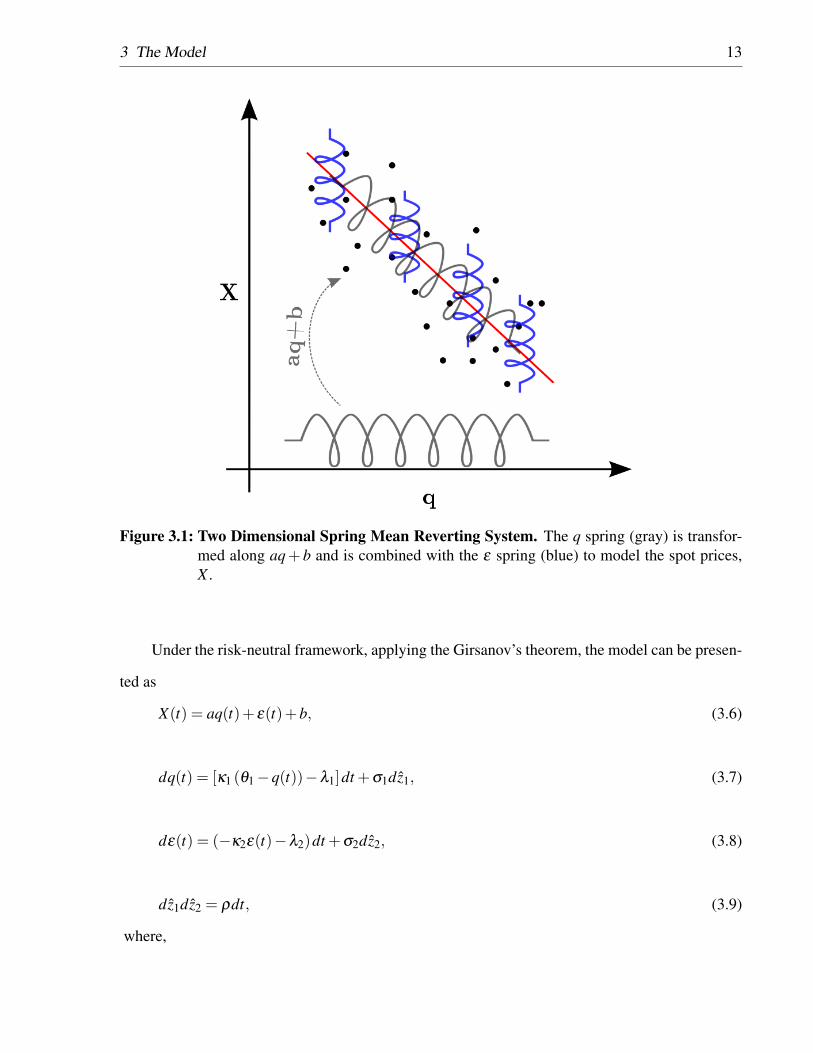
In the proposed model, X is modeled as a 2-dimensional mean reverting system, where the
value of q determines the mean reversion level for X . A 2-dimensional spring system could further
help in understanding the dynamics of this system as demonstrated in figure 3.1. Normalized
excess supply is modeled as a mean reverting process, similar to a spring as shown in figure 3.1,
the gray spring. Furthermore, the ε is also modeled as a mean reverting process, the blue spring,
such that it’s mean reversion (equilibrium) level is zero. In a 2-D spring system, the q spring is
transformed by aq+b such that it lies on the mean reversion level of log-prices.
3 The Model 13
Figure 3.1: Two Dimensional Spring Mean Reverting System. The q spring (gray) is transfor-med along aq+ b and is combined with the ε spring (blue) to model the spot prices,X .
Under the risk-neutral framework, applying the Girsanov’s theorem, the model can be presen-
ted as
X(t) = aq(t)+ ε(t)+b, (3.6)
dq(t) = [κ1 (θ1−q(t))−λ1]dt +σ1dz1, (3.7)
dε(t) = (−κ2ε(t)−λ2)dt +σ2dz2, (3.8)
dz1dz2 = ρdt, (3.9)
where,
3 The Model 14
– z1 and z2 are standard Brownian motions,
– λ1 and λ2 are the market prices of risks.
This joint distribution for q and ε can be then presented as q(t)
ε(t)
∼N
µq(t)
µε(t)
, σ2
q(t) σq(t)ε(t)
σq(t)ε(t) σ2ε(t)
, (3.10)
where N (.) represents a bivariate normal distribution. The terms µq(t), µε(t), σ2q(t), σ2
ε(t), and
σq(t)ε(t) are derived in Appendix 7.1 and presented below
µq(t) = e−κ1 tq(0)+θ1(1− e−κ1 t) , (3.11)
µε(t) = e−κ2 tε(0), (3.12)
σ2q(t) =
12
σ21(1− e−2κ1 t)
κ1, (3.13)
σ2ε(t) =
12
σ22(1− e−2κ2 t)
κ2, (3.14)
σq(t)ε(t) =−σ1 σ2 ρ
(e−t(κ1+κ2)−1
)κ1 +κ2
. (3.15)
The log-spot prices, X , are then normally distributed, N (µX(t),σ2X(t)), with
µX(t) = a((
1− e−tκ1)
θ1 + e−tκ1q(0))+ e−tκ2ε(0)+b, (3.16)
and
σ2X(t) =
a2σ12 (1− e−2 tκ1
)2κ1
+σ2
2 (1− e−2 tκ2)
2κ2+2
aσ1 σ2 ρ
(1− e−t(κ1+κ2)
)κ1 +κ2
. (3.17)
Applying the Feynman-Kac theorem, any derivative under this model should satisfy the fol-
lowing partial differential equation for undiscounted derivatives G
0 = Gt +[κ1(θ1−q)−λ1]Gq +(−κ2ε−λ2)Gε +12
σ21 Gqq +
12
σ22 Gεε +σ1σ2ρGqε . (3.18)
As previously mentioned, we use futures data for calibration of this model. There are two
popualar methods for pricing futures contracts, the expectation method and the no-arbitrage met-
hod. Under the expectation method, for a futures contract, the PDE in equation 3.18 is subject to

3 The Model 15
terminal condition F(T,0) = ST . A futures contract’s value at time t with maturity τ = T − t, de-
noted as F(t,τ), is obtained as the expectation of the spot price at maturity. Given the log-normal
distribution of spot price, we have
F(t,τ) = EQ[S(T )]
= eµQX(T )+
12 σ2
X(T ).
(3.19)
where µQX(T ) is the mean of log-spot price under the risk-neutral measure derived as
µQX(T ) = a
((1− e−(T−t)κ1
)θ1 + e−(T−t)κ1q(t)
)− λ2
κ2
(1− e−(T−t)κ2
)+ e−(T−t)κ2ε(t)+b,
(3.20)
with
θ1 = θ1−λ1
κ1. (3.21)
Substituting for µQX(T ) and σ2
X(T ) in equation 3.19 and reorganizing the equation, we obtain
F(t,τ) = eα(τ)+β (τ)q(t)+γ(τ)ε(t), (3.22)
where
α(τ) = aθ1(1− e−τκ1
)− λ2
κ2
(1− e−τκ2
)+
a2σ12 (1− e−2τκ1
)4κ1
+σ2
2 (1− e−2τκ2)
4κ2
+aσ1 σ2 ρ
(1− e−τ(κ1+κ2)
)κ1 +κ2
+b,
(3.23)
β (τ) = e−κ1τ , (3.24)
and
γ(τ) = e−κ2τ . (3.25)
It should be noted that under these assumptions, log-futures prices follow a normal distribu-
tion N (µF(t,τ),σ2F(t,τ)) with
µF(t,τ) = α(τ)+β (τ)µQq(T )+ γ(τ)µQ
ε(T ), (3.26)
and
σ2F(t,τ) = β (τ)2
σ2q(T )+ γ(τ)2
σ2ε(T )+2β (τ)γ(τ)σq(T )ε(T ). (3.27)
Alternatively, following the no-arbitrage method, the futures price, F(t,τ), is derived as
F(t,τ) = Ste(r−δ )τ , (3.28)
where r is the risk-free interest rate and δ is the net convenience yield for maturity τ . Under
3 The Model 16
the no-arbitrage assumption, log-futures prices follow a similar distribution as the log-spot prices.
Specifically, log-futures are normally distribution, N (µF(t,τ),σ2F(t,τ)) with
µF(t,τ) = µX +(r−δ )τ, (3.29)
and
σ2F(t,τ) = σ
2X . (3.30)
The no-arbitrage and expectation methods should yield consistent results. In theory, changes
in the futures price F(t,τ) should be related to changes in the anticipated distribution of spot
prices at maturity, not the current spot price. However, as suggested in Black (1976), in practice,
the futures prices follow the current spot prices. Black (1976) suggests that changes in the cost of
production, supply, and demand impact both futures and spot prices, resulting in high correlation
between spot and future price changes. Furthermore, events such as the arrival of the production
season only impacts spot prices. Brennan (1958) and Telser (1958) demonstrate that factors such
as interest rates and cost of storage impact futures and spot prices. In light of our aim in this work
to step out of the theoretical realm and model the observed spot-futures relationship, we favor the
no-arbitrage method over the expectation method. In the next section, we present the data used for
calibration.

4 Data
In this section, we apply the proposed model to weekly commodities data from March 1995 to
March 2017. Specifically, crude oil, copper, aluminum , nickel, zinc, tin, and lead futures prices,
production, consumption, and inventory data are used. Futures are available maturing every month
of the year. We select eight futures contracts for calibration of the model, the 1st, 3rd, 6th, 9th,
12th, 15th, 18th, 21st, and 24th nearby contracts. These specific contracts are selected such that
market views and expectations corresponding to the next 8 quarters. Our choice of time frame
is consistent with economic forecasting standards. The selected contracts represent some of the
most highly liquid available contracts. Figure 4.1a represents the maturity of the contracts used for
calibration and WTI prices for sample.
(a) Futures’ Maturity Data (b) Futures’ Price Data
Figure 4.1: WTI Futures Contracts Weekly Information. Weekly West Texas Intermediate fu-tures are used for calibration and estimations from March 1995 to March 2017.
4 Data 18
Moreover, for supply, demand and inventory values, we use data published by international
organizations dedicated to gathering and publishing of such data. Specifically, we use published
reports by the Energy Intelligence Group (EIG) for crude oil and the World Bureau of Metals
Statistics (WBMS) for base metals.
EIG publishes data on global supply and demand on a monthly basis. The inventory data is
only available for the Organization for Economic Cooperation and Development (OECD) coun-
tries, which causes a discrepancy as there are other storage facilities outside of the domain of the
OECD, mainly China, and non-OECD inventory data is not readily available. However, as demon-
strated by Kilian and Murphy (2014), OECD inventory levels provide a good proxy for global oil
inventory levels.
WBMS publishes global supply and demand data for base metals on a monthly basis. Furt-
hermore, base metals’ futures are mainly traded on three exchanges around the world, namely the
Commodity Exchange (COMEX), the London Metal Exchange (LME), and the Shanghai Futures
Exchange (SHFE). These exchanges are the main publicly accessible inventory depots for storage
of base metals. The inventory statistics used in this paper are the cumulative available inventory at
these exchanges.
Figures 4.2a, 4.2b, and 4.2c demonstrate the monthly data on consumption, production, and
inventory. Similar figures for copper, aluminum, nickel, zinc, lead, and tin are presented in the
appendix 7.3.

4 Data 19
(a) Global Crude Oil Consumption Rate (b) Global Crude Oil Production Rate
(c) OECD Countries’ Crude Oil Inventory
Figure 4.2: Crude Oil Consumption, Production, and Inventory Data. Monthly consumption,production, and inventory data are used for estimating normalized excess supply.
Moreover, we obtain U.S. Treasury Rates with maturities ranging from 1 month to 2 years
published by the U.S. Federal Reserve. Then, appropriate interest rates for each specific deriva-
tive’s maturity is calculated via cubic splines. The short term interest rate of less than 1 month
is assumed constant at the 1 month maturity rate. Figure 4.3 demonstrates the yield rates for the
period under study.

4 Data 20
Figure 4.3: US Treasury Rates. T-Rates are used as a proxy for risk-free interest rate in calibra-tion and analysis.
For the purpose of calibration, a Kalman filter process similar to that of Schwartz (1997)
is utilized. The two underlying stochastic factors in the proposed model are normalized excess
supply, q, and the deviation from mean level of log-prices, ε . Spot prices are unobservable for most
commodities. Often, first nearby futures’ prices are used as a proxy for the spot prices. Moreover,
the published supply, demand, and inventory data are only estimates of the true unobservable
variables. This makes straightforward calibration of the processes inaccurate. Hence, the model is
put in a state-space form to account for unknown true values of the state variables. The two state
variables are the q and ε . The Kalman filter is then applied to estimate the true value of the state
variables’ time series. Details of the Kalman filter are presented in Appendix 7.5.

5 Results
In this section, the results of data analysis, model calibration, and scenario analysis are presented.
In section 5.1, we conduct statistical analysis on the constructed normalized excess supply (q) and
deviations from mean (ε) for crude oil. In section 5.2, we presented a sliding window calibration
analysis on crude oil futures. Calibration results are only presented for crude oil for the sake
of brevity and preventing unnecessary repetition. We present results of calibration, in-sample
estimation, and out-of-sample forecasting performance of the model. Additionally, we present out-
of-sample performance of the Schwartz 2-factor model (Schwartz, 1997) for reference. Section 5.3
is dedicated to two case studies, analyzing the out-of-sample performance of the model during the
2008 and 2014 oil market crashes. In section 5.4 we present a scenario analysis framework based
on our model. The framework is of value to risk managers, investment analysts, and traders.
5 Results 22
5.1 Data Analysis
In this section, we analyze the statistical properties of the state variables’ time series for crude oil.
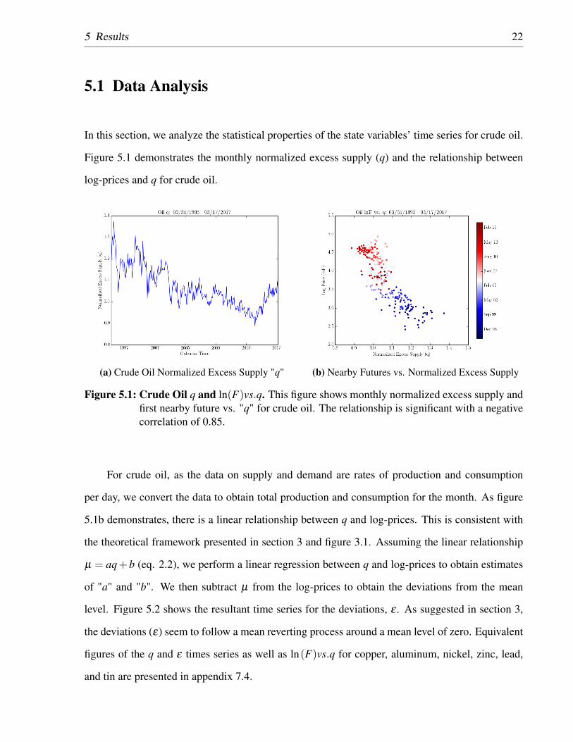
Figure 5.1 demonstrates the monthly normalized excess supply (q) and the relationship between
log-prices and q for crude oil.
(a) Crude Oil Normalized Excess Supply "q" (b) Nearby Futures vs. Normalized Excess Supply
Figure 5.1: Crude Oil q and ln(F)vs.q. This figure shows monthly normalized excess supply andfirst nearby future vs. "q" for crude oil. The relationship is significant with a negativecorrelation of 0.85.
For crude oil, as the data on supply and demand are rates of production and consumption
per day, we convert the data to obtain total production and consumption for the month. As figure
5.1b demonstrates, there is a linear relationship between q and log-prices. This is consistent with
the theoretical framework presented in section 3 and figure 3.1. Assuming the linear relationship
µ = aq+b (eq. 2.2), we perform a linear regression between q and log-prices to obtain estimates
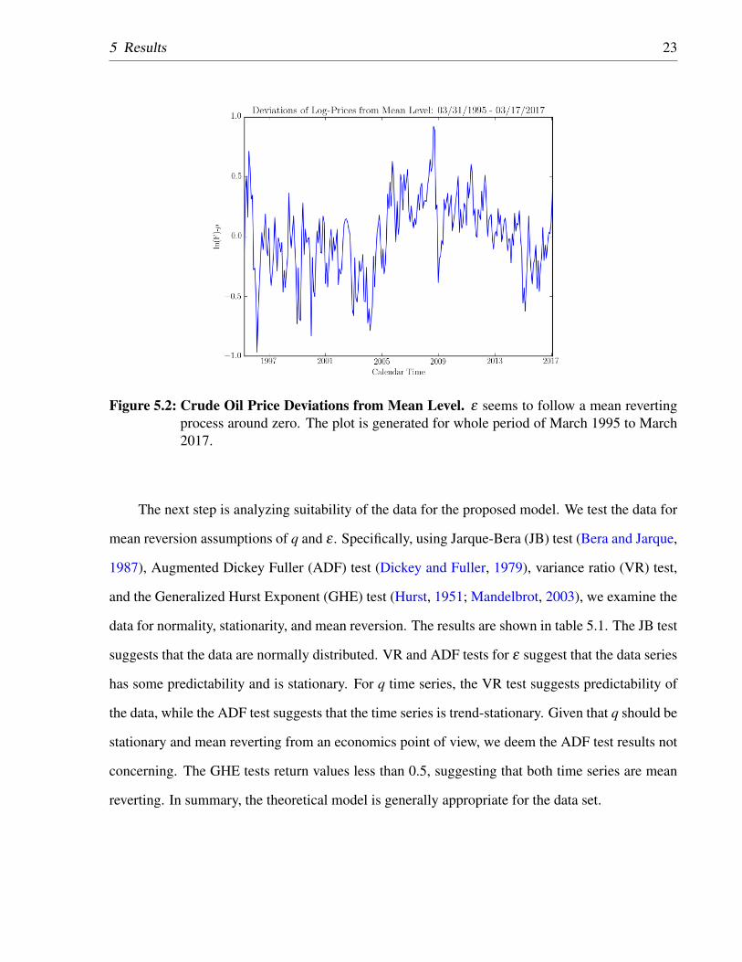
of "a" and "b". We then subtract µ from the log-prices to obtain the deviations from the mean
level. Figure 5.2 shows the resultant time series for the deviations, ε . As suggested in section 3,
the deviations (ε) seem to follow a mean reverting process around a mean level of zero. Equivalent
figures of the q and ε times series as well as ln(F)vs.q for copper, aluminum, nickel, zinc, lead,
and tin are presented in appendix 7.4.
5 Results 23
Figure 5.2: Crude Oil Price Deviations from Mean Level. ε seems to follow a mean revertingprocess around zero. The plot is generated for whole period of March 1995 to March2017.
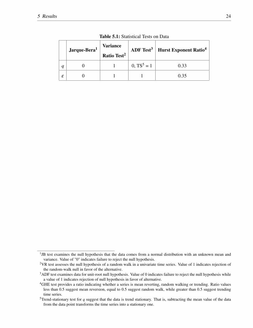
The next step is analyzing suitability of the data for the proposed model. We test the data for
mean reversion assumptions of q and ε . Specifically, using Jarque-Bera (JB) test (Bera and Jarque,
1987), Augmented Dickey Fuller (ADF) test (Dickey and Fuller, 1979), variance ratio (VR) test,
and the Generalized Hurst Exponent (GHE) test (Hurst, 1951; Mandelbrot, 2003), we examine the
data for normality, stationarity, and mean reversion. The results are shown in table 5.1. The JB test
suggests that the data are normally distributed. VR and ADF tests for ε suggest that the data series
has some predictability and is stationary. For q time series, the VR test suggests predictability of
the data, while the ADF test suggests that the time series is trend-stationary. Given that q should be
stationary and mean reverting from an economics point of view, we deem the ADF test results not
concerning. The GHE tests return values less than 0.5, suggesting that both time series are mean
reverting. In summary, the theoretical model is generally appropriate for the data set.
5 Results 24
Table 5.1: Statistical Tests on Data
Jarque-Bera1 Variance
Ratio Test2ADF Test3 Hurst Exponent Ratio4
q 0 1 0, TS5 = 1 0.33
ε 0 1 1 0.35
1JB test examines the null hypothesis that the data comes from a normal distribution with an unknown mean andvariance. Value of "0" indicates failure to reject the null hypothesis.
2VR test assesses the null hypothesis of a random walk in a univariate time series. Value of 1 indicates rejection ofthe random-walk null in favor of the alternative.
3ADF test examines data for unit-root null hypothesis. Value of 0 indicates failure to reject the null hypothesis whilea value of 1 indicates rejection of null hypothesis in favor of alternative.
4GHE test provides a ratio indicating whether a series is mean reverting, random walking or trending. Ratio valuesless than 0.5 suggest mean reversion, equal to 0.5 suggest random walk, while greater than 0.5 suggest trendingtime series.
5Trend-stationary test for q suggest that the data is trend stationary. That is, subtracting the mean value of the datafrom the data point transforms the time series into a stationary one.

5 Results 25
5.2 Calibration
For the purpose of calibration, we follow the process set out in appendix 7.5. Specifically, we use
two rolling windows and an expanding window frame works to calibrate and test the model and
analyze the results. We implement three tests; One with a 3 year rolling window, one with a 5
year rolling window, and one with an expanding window. The windows move on monthly basis as
shown in figure 5.3. These configurations resulted in respectively 250, 227, and 251 windows and
instances of calibration for the 3 year, 5 year, and expanding windows alternatives.
Figure 5.3: Rolling and Expanding Window Calibrations. Rolling windows of 3 and 5 yearsand an expanding window are used for calibration. The windows slide one month at atime. The frequency of data used for calibration is weekly.
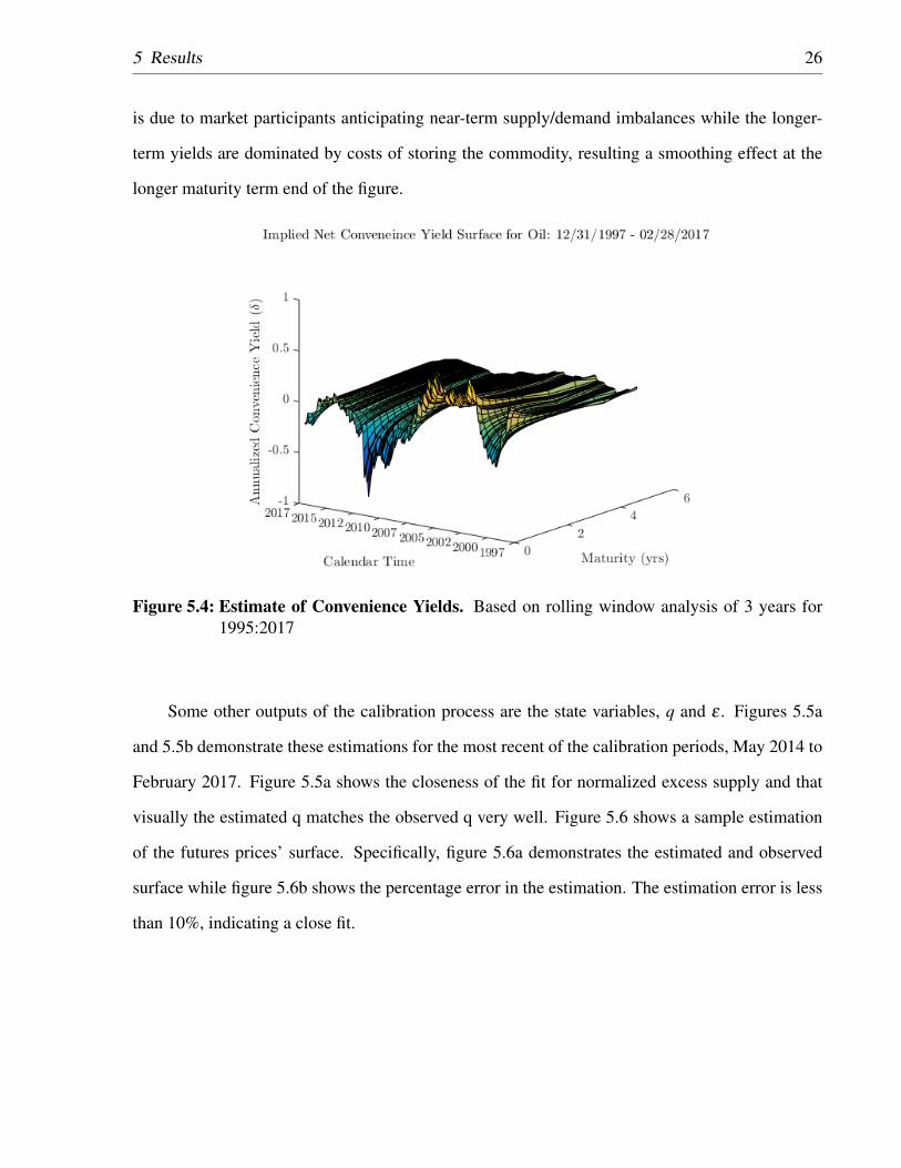
One of the outputs of our calibration is the set of convenience yields of equation 3.28 as-
sociated with each contract, at each point in time. This convenience yield is the yield net of any
costs associated with holding the commodity such as storage costs, insurance, and spoilage. Figure
5.4 demonstrates the annualized market implied net convenience yield. As expected, the conve-
nience yield is more volatile in the short-term and plateaus as the term to maturity increases. This
5 Results 26
is due to market participants anticipating near-term supply/demand imbalances while the longer-
term yields are dominated by costs of storing the commodity, resulting a smoothing effect at the
longer maturity term end of the figure.
Figure 5.4: Estimate of Convenience Yields. Based on rolling window analysis of 3 years for1995:2017
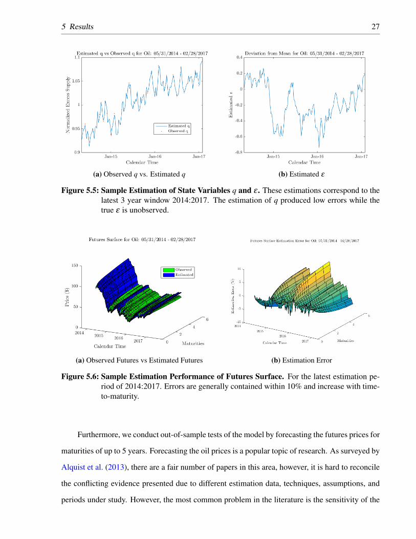
Some other outputs of the calibration process are the state variables, q and ε . Figures 5.5a
and 5.5b demonstrate these estimations for the most recent of the calibration periods, May 2014 to
February 2017. Figure 5.5a shows the closeness of the fit for normalized excess supply and that
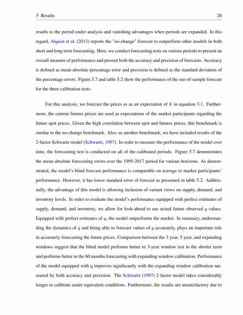
visually the estimated q matches the observed q very well. Figure 5.6 shows a sample estimation
of the futures prices’ surface. Specifically, figure 5.6a demonstrates the estimated and observed
surface while figure 5.6b shows the percentage error in the estimation. The estimation error is less
than 10%, indicating a close fit.
5 Results 27
(a) Observed q vs. Estimated q (b) Estimated ε
Figure 5.5: Sample Estimation of State Variables q and ε . These estimations correspond to thelatest 3 year window 2014:2017. The estimation of q produced low errors while thetrue ε is unobserved.
(a) Observed Futures vs Estimated Futures (b) Estimation Error
Figure 5.6: Sample Estimation Performance of Futures Surface. For the latest estimation pe-riod of 2014:2017. Errors are generally contained within 10% and increase with time-to-maturity.
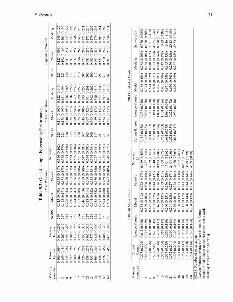
Furthermore, we conduct out-of-sample tests of the model by forecasting the futures prices for
maturities of up to 5 years. Forecasting the oil prices is a popular topic of research. As surveyed by
Alquist et al. (2013), there are a fair number of papers in this area, however, it is hard to reconcile
the conflicting evidence presented due to different estimation data, techniques, assumptions, and
periods under study. However, the most common problem in the literature is the sensitivity of the
5 Results 28
results to the period under analysis and vanishing advantages when periods are expanded. In this
regard, Alquist et al. (2013) reports the "no-change" forecast to outperform other models in both
short and long term forecasting. Here, we conduct forecasting tests on various periods to present an
overall measure of performance and present both the accuracy and precision of forecasts. Accuracy
is defined as mean absolute percentage error and precision is defined as the standard deviation of
the percentage errors. Figure 5.7 and table 5.2 show the performance of the out-of-sample forecast
for the three calibration tests.
For this analysis, we forecast the prices as as an expectation of X in equation 3.1. Further-
more, the current futures prices are used as expectations of the market participants regarding the
future spot prices. Given the high correlation between spot and futures prices, this benchmark is
similar to the no-change benchmark. Also, as another benchmark, we have included results of the
2-factor Schwartz model (Schwartz, 1997). In order to measure the performance of the model over
time, the forecasting test is conducted on all of the calibrated periods. Figure 5.7 demonstrates
the mean absolute forecasting errors over the 1995-2017 period for various horizons. As demon-
strated, the model’s blind forecast performance is comparable on average to market participants’
performance. However, it has lower standard error of forecast as presented in table 5.2. Additio-
nally, the advantage of this model is allowing inclusion of variant views on supply, demand, and
inventory levels. In order to evaluate the model’s performance equipped with perfect estimates of
supply, demand, and inventory, we allow for look-ahead to use actual future observed q values.
Equipped with perfect estimates of q, the model outperforms the market. In summary, understan-
ding the dynamics of q and being able to forecast values of q accurately, plays an important role
in accurately forecasting the future prices. Comparison between the 3 year, 5 year, and expanding
windows suggest that the blind model performs better in 3-year window test in the shorter term
and performs better in the 60 months forecasting with expanding window calibration. Performance
of the model equipped with q improves significantly with the expanding window calibration me-
asured by both accuracy and precision. The Schwartz (1997) 2 factor model takes considerably
longer to calibrate under equivalent conditions. Furthermore, the results are unsatisfactory due to

5 Results 29
low accuracy and precision. We have limited the Y-Axis in figures 5.7 to highlight the distinctions
of different models and calibration setups.

5 Results 30
(a) 3 year window calibration
(b) 5 year window calibration
(c) Expanding window calibration
Figure 5.7: Out-of-sample Forecasting Performance. Figures above demonstrate the mean ab-solute percentage error of forecasts under different calibration setups and time hori-zons.
5 Results 31
Tabl
e5.
2:O
ut-o
f-sa
mpl
eFo
reca
stin
gPe
rfor
man
ce3
Yea
rWin
dow
s5
Yea
rWin
dow
sE
xpan
ding
Win
dow
Mat
urity
(mon
ths)
Cur
rent
Futu
res
Ave
rage
Futu
res
NO
BS
Mod
elM
odel
qSc
hwar
tz2F
NO
BS
Mod
elM
odel
qN
OB
SM
odel
Mod
elq
10.
106
(0.0
94)
0.16
4(0
.204
)24
90.
115
(0.0
98)
0.13
3(0
.117
)0.
166
(0.1
62)
225
0.11
1(0
.100
)0.
122
(0.1
16)
225
0.12
5(0
.099
)0.
148
(0.1
27)
30.
159
(0.1
86)
0.20
7(0
.249
)24
70.
173
(0.1
71)
0.18
4(0
.175
)0.
333
(0.3
70)
223
0.17
3(0
.197
)0.
181
(0.1
96)
223
0.19
2(0
.166
)0.
201
(0.1
90)
60.
225
(0.2
87)
0.25
4(0
.276
)24
40.
228
(0.2
52)
0.22
0(0
.237
)0.
494
(0.5
58)
220
0.24
0(0
.293
)0.
238
(0.2
85)
220
0.25
4(0
.231
)0.
237
(0.2
29)
90.
259
(0.2
65)
0.28
8(0
.270
)24
10.
260
(0.2
53)
0.22
5(0
.235
)0.
554
(0.5
59)
217
0.27
5(0
.270
)0.
256
(0.2
56)
217
0.29
7(0
.242
)0.
243
(0.2
06)
120.
280
(0.2
50)
0.31
2(0
.293
)23
70.
274
(0.2
47)
0.23
6(0
.239
)0.
565
(0.5
84)
213
0.29
9(0
.248
)0.
262
(0.2
32)
213
0.33
2(0
.25)
0.24
6(0
.200
)15
0.30
4(0
.268
)0.
329
(0.3
17)
234
0.29
7(0
.289
)0.
266
(0.2
86)
0.55
1(0
.583
)21
00.
325
(0.2
87)
0.27
9(0
.258
)21
00.
356
(0.2
66)
0.26
3(0
.210
)18
0.32
6(0
.282
)0.
352
(0.3
33)
231
0.31
6(0
.310
)0.
289
(0.3
08)
0.54
7(0
.597
)20
70.
345
(0.3
06)
0.29
3(0
.257
)20
70.
372
(0.2
89)
0.27
1(0
.221
)21
0.33
8(0
.277
)0.
367
(0.3
35)
227
0.32
8(0
.314
)0.
300
(0.3
14)
0.54
4(0
.593
)20
30.
367
(0.3
23)
0.30
1(0
.261
)20
30.
381
(0.2
85)
0.27
1(0
.214
)24
0.35
3(0
.278
)0.
377
(0.3
46)
224
0.34
4(0
.322
)0.
318
(0.3
34)
0.54
4(0
.544
)20
00.
393
(0.3
40)
0.30
2(0
.262
)20
00.
403
(0.2
88)
0.27
9(0
.207
)36
0.36
5(0
.366
)0.
436
(0.4
00)
122
0.38
8(0
.352
)0.
380
(0.3
56)
0.72
7(0
.744
)11
70.
489
(0.4
76)
0.32
0(0
.313
)11
70.
494
(0.3
54)
0.27
9(0
.233
)48
0.44
8(0
.438
)0.
494
(0.4
29)
102
0.47
7(0
.442
)0.
416
(0.3
30)
0.77
1(0
.699
)99
0.55
3(0
.442
)0.
377
(0.3
31)
990.
521
(0.3
66)
0.30
4(0
.281
)59
0.52
6(0
.454
)0.
488
(0.3
70)
930.
544
(0.4
80)
0.46
9(0
.389
)0.
735
(0.6
21)
910.
554
(0.3
52)
0.39
7(0
.310
)91
0.51
0(0
.242
)0.
331
(0.2
62)
600.
519
(0.4
53)
0.47
7(0
.362
)89
0.53
9(0
.489
)0.
477
(0.4
05)
0.74
5(0
.671
)86
0.55
1(0
.338
)0.
401
(0.3
17)
860.
507
(0.2
38)
0.33
6(0
.271
)
2008
Oil
Mar
ketC
rash
2014
Oil
Mar
ketC
rash
Mat
urity
(mon
ths)
Cur
rent
Futu
res
Ave
rage
Futu
res
Mod
elM
odel
qSc
hwar
tz2F
Cur
rent
Futu
res
Ave
rage
Futu
res
Mod
elM
odel
qSc
hwar
tz2F
10.
275
(0.2
24)
0.64
2(0
.600
)0.
254
(0.2
12)
0.27
2(0
.271
)0.
619
(0.4
59)
0.18
7(0
.138
)0.
338
(0.3
10)
0.18
2(0
.164
)0.
268
(0.2
65)
0.33
6(0
.250
)3
0.56
(0.4
99)
0.77
3(0
.639
)0.
509
(0.4
02)
0.50
8(0
.456
)1.
777
(1.1
46)
0.36
3(0
.233
)0.
503
(0.3
36)
0.39
4(0
.258
)0.
468
(0.4
04)
0.96
6(0
.565
)6
0.79
7(0
.776
)0.
807
(0.5
90)
0.67
7(0
.559
)0.
658
(0.5
68)
4.02
9(1
.953
)0.
481
(0.3
22)
0.71
2(0
.260
)0.
544
(0.3
29)
0.44
0(0
.475
)2.
351
(2.4
10)
90.
57(0
.549
)0.
576
(0.3
45)
0.46
3(0
.325
)0.
414
(0.4
22)
5.94
0(2
.147
)0.
583
(0.1
89)
0.86
1(0
.160
)0.
688
(0.2
71)
0.38
3(0
.250
)4.
735
(7.6
44)
120.
428
(0.3
14)
0.43
7(0
.197
)0.
346
(0.1
50)
0.28
6(0
.196
)8.
123
(4.0
01)
0.70
7(0
.296
)1.
024
(0.4
20)
0.80
6(0
.301
)0.
430
(0.2
69)
8.57
8(2
0.21
)15
0.37
2(0
.264
)0.
369
(0.1
87)
0.29
5(0
.137
)0.
293
(0.2
14)
11.6
8(6
.678
)0.
752
(0.5
03)
1.10
1(0
.586
)0.
901
(0.5
06)
0.44
7(0
.278
)10
.83
(24.
99)
180.
337
(0.2
43)
0.36
0(0
.160
)0.
290
(0.1
31)
0.27
6(0
.238
)17
.01
(12.
62)
0.69
1(0
.573
)1.
080
(0.6
44)
0.87
1(0
.538
)0.
395
(0.3
33)
16.1
6(4
8.18
)21
0.35
2(0
.201
)0.
390
(0.1
63)
0.29
1(0
.138
)0.
227
(0.1
74)
24.0
4(2
0.06
)0.
521
(0.3
34)
0.82
2(0
.472
)0.
650
(0.3
63)
0.27
6(0
.156
)20
.13
(66.
39)
240.
403
(0.2
04)
0.39
0(0
.164
)0.
335
(0.1
61)
0.32
2(0
.184
)31
.76
(28.
09)
0.61
5(0
.347
)0.
930
(0.3
10)
0.67
9(0
.299
)0.
267
(0.1
55)
29.8
4(1
09.4
)36
0.31
4(0
.106
)0.
296
(0.1
70)
0.30
6(0
.149
)0.
263
(0.1
36)
123.
2(1
48.4
)48
0.25
7(0
.147
)0.
287
(0.1
14)
0.21
7(0
.115
)0.
143
(0.1
50)
663.
7(1
025)
590.
237
(0.1
28)
0.22
8(0
.153
)0.
200
(0.1
40)
0.14
4(0
.145
)35
79(7
229)
600.
224
(0.1
14)
0.22
6(0
.164
)0.
204
(0.1
29)
0.15
6(0
.144
)42
69(9
179)
NO
BS:
Num
bero
fobs
erva
tions
Ave
rage
Futu
res:
Ave
rage
ofpa
st6
mon
ths
futu
res
Mod
el:B
lind
2fa
ctor
mod
elpr
esen
ted
inth
isw
ork
Mod
elq:
Fore
cast
with
know
nq
5 Results 32
5.3 Case Analysis - Oil Market Crashes
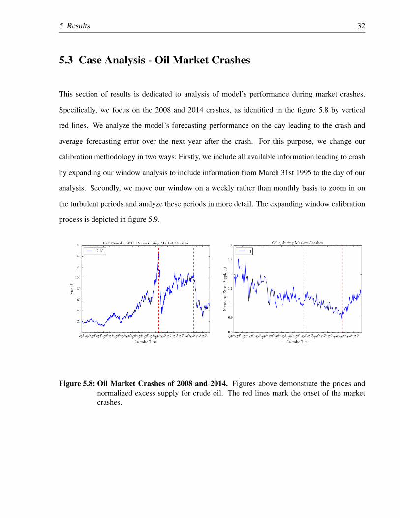
This section of results is dedicated to analysis of model’s performance during market crashes.
Specifically, we focus on the 2008 and 2014 crashes, as identified in the figure 5.8 by vertical
red lines. We analyze the model’s forecasting performance on the day leading to the crash and
average forecasting error over the next year after the crash. For this purpose, we change our
calibration methodology in two ways; Firstly, we include all available information leading to crash
by expanding our window analysis to include information from March 31st 1995 to the day of our
analysis. Secondly, we move our window on a weekly rather than monthly basis to zoom in on
the turbulent periods and analyze these periods in more detail. The expanding window calibration
process is depicted in figure 5.9.
Figure 5.8: Oil Market Crashes of 2008 and 2014. Figures above demonstrate the prices andnormalized excess supply for crude oil. The red lines mark the onset of the marketcrashes.

5 Results 33
Figure 5.9: Expanding Window Example. The calibration window is moved one week at a time,beginning from the onset of the crash (red line) to the 1 year mark after crash (blackline).
5.3.1 2008 Market Crash
The year 2008 witnessed massive swings in crude oil prices with prices reaching a peak of $145
and crashing to a low of $32. On July 15th 2008, the sell-off began and continued throughout the
year. It is believed that executive order signed by the United State’s president George W. Bush on
July 15th lifting the ban on off-shore drilling initiated the sell-off. In the following months, easing
of tensions between U.S. and Iran (July 2008) , Lehman Brothers bankruptcy (September 2008), a
stronger U.S. Dollar (October 2008), decline in demand from the European Zone (October 2008),
and increasing U.S. unemployment rate combined with weak economic data (November 2008) led
to prices falling to $32 by the end of 2008.
5 Results 34
5.3.2 2014 Market Crash
The year 2014 was filled with geopolitical tensions impacting oil prices. Commencement of the
Joint Action Plan for Iran’s nuclear program (January 2014), war in the middle east (Syria, Lybia,
...), and the dispute over Crimea and annexation of Crimea by Russia (February-March 2014) are
among the headlines impacting oil prices in 2014. Finally in June 2014 the oil market boiled over
and begun the recent crash. Increasing U.S. shale and light oil production, decreasing demand
from China and the European Zone, and OPEC’s inability to reach a deal over production cuts lead
to oil prices crashing from $106 to $45 by the end of 2014.
5.3.3 Results During Market Crash Periods
Results of the out-of-sample forecasting for the two periods are presented in figure 5.10 and table
5.2. Figures 5.10a and 5.10c represent the actual out-of-sample forecasts on the day the crashes
begun. For the 2008 crash, we can forecast up to 5 years while for the 2014 crash we could only
extend the forecast horizon to two years. During both crashes, the model equipped with "q" infor-
mation follows the prices closely, beating all other benchmarks. The blind model’s performance
is different during the two crashes. During the 2008 crash, the blind model forecasts the correct
shape for prices and follows the trends while the forecasts are close to market expectations during
the 2014 crash.
Furthermore, figures 5.10b and 5.10d present the average forecasts error for a 52-week period
following the crash. Similarly, the results follow the same trends; The model equipped with "q"
outperforms all the benchmarks while the blind model produces results with similar accuracy as
the benchmark. In terms of standard error of forecasts, both the blind model and the model with q
produce results with lower standard errors.

5 Results 35
(a) (b)
(c) (d)
Figure 5.10: Out-of-sample Forecasting Performance During Market Crashes of 2008 and2014. Figures on the left demonstrate the out-of-sample forecasts on the onset of themarket crashes while the figures on the right represent the mean absolute percentageerror during one year after the crash.
5 Results 36
5.4 Scenario Analysis
In this section, we analyze the utility of our model for scenario analysis. As mention before, a
unique contribution of the proposed model is the ability to analyze the impact of supply, demand,
and inventory changes on values of derivatives such as futures contracts and options on futures
contracts. Specifically, in light of ever-changing macroeconomic conditions, analysts can develop
variant views of future consumption and production trends for the commodity. For instance, in case
of Chinese economy’s transition to consumerism, analysts can build scenarios for oil consumption
trends and analyze the impact on commodity spot and derivative prices. Another example is the ge-
opolitical tensions underlying oil production within OPEC countries. Deals regarding production
quotas made under political tensions are fragile and not adhering to quotas could result in invest-
ment losses and increased risks for investors. In order to build out scenarios, assuming the current
time period is denoted by "t", analysts can forecast variables in the following framework:
1. Forecast production for period t +1.
2. Forecast consumption for period t +1.
3. Adjust ending inventory for period t +1 as
Inventoryt+1 = Inventoryt +Productiont+1−Consumptiont+1. (5.1)
4. Forecast production and consumption for period t + 2, taking into account producers’ and
consumers’ reactions to the updated level of inventory and macroeconomic conditions.
5. Adjust ending inventory for period t +2, and repeat as necessary.
This framework is valuable to risk managers as well, providing a tool to hedge positions in
the face of uncertain macroeconomic and political adversities. Here, we present an example of this
framework applied to a series of positive shocks to oil production. Specifically, we develop two
scenarios .

5 Results 37
1. Scenario 1: Oil consumption and production continue their long-term trends assuming a
linear model.
2. Scenario 2: We assume an initial breach in the recent OPEC production deal by a single
member leading to increased production by all members over the next 12 months. The
scenario is constructed as below.
i Total production increases by 112 million barrels per day, every month, for the next 12
months, as demonstrated in 5.11a.
ii Consumption trend is assumed unchanged, as demonstrated in 5.11b.
iii Inventory is built up periodically due to increased productionas demonstrated in 5.11c.
iv An oil glut is made due to increased inventory and production. A new deal is reached
bringing the production back to normal levels, a reduction of 1 million barrels per day
by OPEC members.
v Moreover, higher cost producers exit the market due to lower prices, reducing the pro-
duction by another 0.5 million barrels per day.
Figure 5.11 demonstrates the two scenarios. Figure 5.11a compares the progress of production
rate under the two scenarios, while figure 5.11b shows the steady consumption increases. Figures
5.11c and 5.11d show the inventory built up and impact on the normalized excess supply over the
next two years.

5 Results 38
(a) (b)
(c) (d)
Figure 5.11: Scenario Analysis for increased production. The figures above present the pro-duction, consumption, inventory levels, and normalized excess supply under bothscenarios. Values before January 2017 are historical values while the data after thatis generated based on the scenarios.
Assuming the two scenarios, we can now forecast the spot prices. Figure 5.12 demonstrates
the foretasted spot prices under both scenarios. Under the first scenario, production outpaced con-
sumption, leading to significant price falls. Under the second scenario, extra production increases
led to a sharper price decrease compared to the first scenario. However, after the first year, with the
new OPEC deal and lower production of higher cost producers, total production falls by 1.5 million
barrels per day. The production decrease leads to falling q and inventory levels while increasing
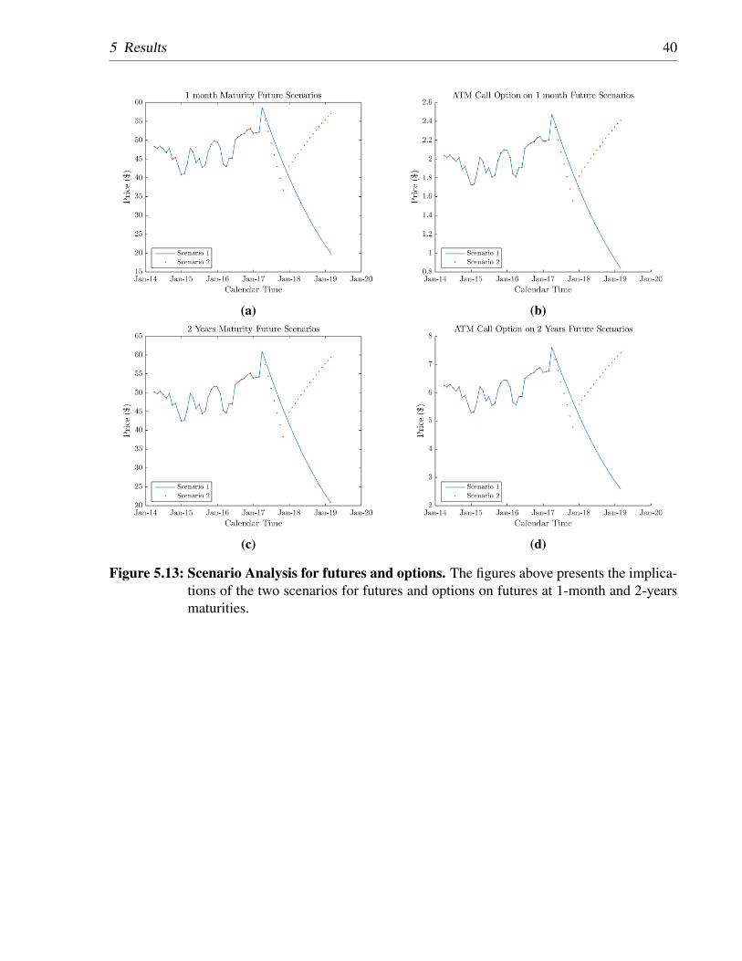
prices. Furthermore, we can now estimate futures prices and options on futures. Figure 5.13 de-

5 Results 39
monstrates the impact of scenarios on futures and options contracts. Specifically, we demonstrate
the impact on constant maturity maturity futures contracts as well as the impact on at-the-money
(ATM) call options on these futures contracts. The options are assumed to have the same maturity
as the futures. Figures 5.13a and 5.13b demonstrate the impact on a short term 1 month maturity
futures contract and the related ATM call option. Similarly, figures 5.13c and 5.13d demonstrate
the impact on a 2 years maturity futures contract and the related ATM call option. Similar to spot
prices, the futures prices and option prices fall under the first scenario, while the fall is sharper and
is followed by a bounce back under the second scenario.
Figure 5.12: Scenario Analysis of Spot Prices. This figure presents the spot prices under thetwo proposed scenarios. Spot prices prior to January 2017 are results of calibration,combination of the two state variables in Kalman filter. Prices after January 2017are produced under the two scenarios with model parameters calibrated to the latestperiod.
5 Results 40
(a) (b)
(c) (d)
Figure 5.13: Scenario Analysis for futures and options. The figures above presents the implica-tions of the two scenarios for futures and options on futures at 1-month and 2-yearsmaturities.
6 Conclusions
In this paper, we put forward a framework to capture the observed dynamics between prices, sup-
ply/demand, and inventories. Specifically, normalized excess supply is proposed as the ratio of
total excess supply to total demand. We show that normalized excess supply and log-prices follow
an inverse linear relationship, consistent with economic theory of supply and demand. Further-
more, we show that normalized excess supply follows a mean reverting process. We propose that
normalized excess supply determines the mean level of log-spot prices. In addition, deviations of
prices from the mean level follow a mean reverting process. We utilize the aforementioned pro-
perties to develop a two factor stochastic model for estimation of storable commodity spot prices,
with application in derivatives’ valuations. The two stochastic factors of our model are normalized
excess supply and the deviations from the mean level. Additionally, we develop two futures prices
formulas based on the expectation theory as well as the no-arbitrage theory.
We calibrate the model to crude oil market data from March 1995 to March 2017 using a
Kalman filter under three calibration setups; A 3-year rolling window, a 5-year rolling window, and
an expanding window. We back test the model for both in-sample and out-of-sample data. We show
that the proposed model matches the in-sample futures data very well and outperforms the market
in out-of-sample foretasting of spot prices. Furthermore, we apply the model to the oil market
crashes of 2008 and 2014, and demonstrate the models superiority in both accuracy and precision
of out-of-sample forecasts. Additionally, we develop a scenario analysis framework to incorporate
variant views of future production, consumption, and inventory levels into forecasting of spot

6 Conclusions 42
prices. We further demonstrated the impact of the scenarios on futures and options on futures
contracts. The spot, futures contracts, and option contracts prices are consistent with economic
theory of supply and demand. We show the scenario analysis framework to be a valuable toolkit for
investment management professionals and risk/quantitative analysts, allowing them to incorporate
their views on macroeconomic developments in forecasting prices and valuations of investments.
References
Alquist, R., Kilian, L., and Vigfusson, R. J. (2013). Forecasting the Price of Oil. In Handbook of
Economic Forecasting, pages 427–507.
Arismendi, J. C., Back, J., Prokopczuk, M., Paschke, R., and Rudolf, M. (2016). Seasonal sto-
chastic volatility: Implications for the pricing of commodity options. Journal of Banking &
Finance.
Bastian-Pinto, C., Brandão, L., and Hahn, W. J. (2009). Flexibility as a source of value in the
production of alternative fuels : The ethanol case. Energy Economics, 31(3):411–422.
Baumeister, C. and Kilian, L. (2016). Real-Time Forecasts of the Real Price of Oil Real-Time
Forecasts of the Real Price of Oil. Journal of Business & Economic Statistics, 30(2):326–336.
Beckmann, J., Belke, A., and Czudaj, R. (2014). Does global liquidity drive commodity prices?
Journal of Banking and Finance, 48:224–234.
Belousova, J. and Dorfleitner, G. (2012). On the diversification benefits of commodities from the
perspective of euro investors. Journal of Banking and Finance, 36(9):2455–2472.
Bera, A. K. and Jarque, C. M. (1987). A Test for Normality of Observations and Regression
Residuals. International Statistical Review, 55(2):163–172.
BIS (2015). Semiannual OTC derivatives statistics. Technical report, Bank for International Sett-
lements.
References 44
Black, F. (1976). The Pricing of Commodity Contracts. Journal of Financial Economics, 3:167–
179.
Brandão, L. E. T., Penedo, G. M., and Bastian-Pinto, C. (2013). The value of switching inputs in
a biodiesel production plant. The European Journal of Finance, 2013, 19(7-8):674–688.
Brennan, M. J. (1958). The Supply of Storage. American Economic Review, 48(1):50–72.
Bu, H. (2014). Effect of Inventory Announcements on Crude Oil Price Volatility. Energy Econo-
mics, 46:485–494.
Carlson, M., Khokher, Z., and Titman, S. (2007). Resource Price Dynamics. The Journal of
Finance, LXII(4):1663–1703.
Casassus, J. and Collin-Dufresne, P. (2005). Stochastic Convenience Yield Implied from Commo-
dity Futures and Interest Rates. The Journal of Finance, 60(5):2283–2331.
Casassus, J., Liu, P., and Tang, K. (2013). Economic linkages, relative scarcity, and commodity
futures returns. Review of Financial Studies, 26(5):1324–1362.
Chen, S. and Insley, M. (2012). Regime switching in stochastic models of commodity prices: An
application to an optimal tree harvesting problem. Journal of Economic Dynamics and Control,
36(2):201–219.
Chiang, I.-h. E., Hughen, W. K., and Sagi, J. S. (2015). Estimating Oil Risk Factors Using Infor-
mation from Equity and Derivatives Markets. The Journal of Finance, LXX(2):769–804.
Cuñado, J. and de Gracia, F. P. (2003). Do oil price shocks matter? Evidence for some European
countries. Energy Economics, 25(2):137–154.
Dickey, D. A. and Fuller, W. A. (1979). Distribution of the Estimators for Autoregressive Time
Series With a Unit Root. Journal of the American Statistical Association, 74(366):427–431.
Ebert, L. and La Menza, T. (2015). Chile, copper and resource revenue: A holistic approach to
assessing commodity dependence. Resources Policy, 43:101–111.
References 45
Elder, J., Miao, H., and Ramchander, S. (2012). Impact of macroeconomic news on metal futures.
Journal of Banking and Finance, 36(1):51–65.
Erb, C. B. and Harvey, C. R. (2006). The Strategic and Tactical Value of Commodity Futures.
Financial Analysts Journal, 62(2):69–97.
Geman, H. (2005). Commodities and Commodity Derivatives: Modeling and Pricing for Agricul-
turals, Metals and Energy. Wiley & Sons, Ltd., Chichester, West Sussex, England.
Geman, H. and Smith, W. O. (2013). Theory of storage, inventory and volatility in the LME base
metals. Resources Policy, 38(1):18–28.
Gibson, R. and Schwartz, E. S. (1990). Stochastic Convenience Yield and the Pricing of Oil
Contingent Claims.
Gorton, G. and Rouwenhorst, K. G. (2006). Facts and Fantasies about Commodity Futures. Fi-
nancial Analysts Journal, 62(2):47–68.
Greer, R. J. (2000). The Nature of Commodity Index Returns. THE JOURNAL OF ALTERNATIVE
INVESTMENTS, 3:45–53.
Güntner, J. H. F. (2014). How do oil producers respond to oil demand shocks ? Energy Economics,
44:1–13.
Hamilton, J. D. (2008). Oil and the Macroeconomy. In Durlauf, S. N. and Blume, L. E., editors,
In The New Palgrave Dictionary of Economics. Palgrave Macmillan, 2 edition.
Hamilton, J. D. (2011). Nonlinearities and the Macroeconomic Effects of Oil Prices. Macroeco-
nomic Dynamics, 15(Supplement 3):364–378.
Hikspoors, S. and Jaimungal, S. (2008). Asymptotic Pricing of Commodity Derivatives using
Stochastic Volatility Spot Models. Applied Mathematical Finance, 15(5-6):449–477.
Hong, H. and Yogo, M. (2012). What does futures market interest tell us about the macroeconomy
and asset prices? Journal of Financial Economics, 105(3):473–490.

References 46
Hurst, H. E. (1951). Long-term storage capacity of reservoirs. Transactions of American Society
of Civil Engineers, 116:770–808.
Irwin, S. H. and Sanders, D. R. (2011). Index funds, financialization, and commodity futures
markets. Applied Economic Perspectives and Policy, 33(1):1–31.
Juvenal, L. and Petrella, I. (2015). Speculation in the Oil Market. Journal of Applied Econometrics,
30(4):621–649.
Kaminski, V. (2014). The microstructure of the North American oil market. Energy Economics,
46:S1–S10.
Kilian, L. (2014). Oil Price Shocks : Causes and Consequences. The Annual Review of Resource
Economics, 6:133–154.
Kilian, L. and Lee, T. K. (2014). Quantifying the speculative component in the real price of oil:
The role of global oil inventories. Journal of International Money and Finance, 42:71–87.
Kilian, L. and Murphy, D. P. (2014). The Role of Inventories and Speculative Trading in the Global
Market for Crude Oil. Journal of Applied Econometrics, 29(3):454–478.
Kobari, L., Jaimungal, S., and Lawryshyn, Y. (2014). A real options model to evaluate the effect
of environmental policies on the oil sands rate of expansion. Energy Economics, 45:155–165.
Lai, A. N. and Mellios, C. (2016). Valuation of commodity derivatives with an unobservable
convenience yield. Computers and Operations Research, 66:402–414.
Liu, P. and Tang, K. (2011). The stochastic behavior of commodity prices with heteroskedasticity
in the convenience yield. Journal of Empirical Finance, 18(2):211–224.
Mandelbrot, B. B. (2003). Heavy Tails in Finance for Independent or Multifractal Price Increments.
In S.T. Rachev, editor, Handbook of Heavy Tailed Distributions in Finance, chapter 1. Elsevier
Science B.V.

References 47
Mirantes, A. G., Población, J., and Serna, G. (2013). The stochastic seasonal behavior of energy
commodity convenience yields. Energy Economics, 40:155–166.
Morana, C. (2013). The Oil Price-Macroeconomy Relationship Since the Mid-1980s: A Global
Perspective. The Energy Journal, 34(3):153–189.
Paschke, R. and Prokopczuk, M. (2010). Commodity derivatives valuation with autoregressive
and moving average components in the price dynamics. Journal of Banking and Finance,
34(11):2742–2752.
Ratti, R. A. and Vespignani, J. L. (2015). Commodity prices and BRIC and G3 liquidity: A
SFAVEC approach. Journal of Banking and Finance, 53:18–33.
Routledge, B. R., Seppi, D. J., and Spatt, C. S. (2000). Equilibrium Forward Curves for Commo-
dities. The Journal of Finance, LV(3):1297–1338.
Schwartz, E. S. (1997). The Stochastic Behavior of Commodity Prices: Implications for Valuation
and Hedging. The journal of Finance, 52(3):923 – 973.
Sidebottom, A., Belur, J., Bowers, K., Tompson, L., and Johnson, S. D. (2011). Theft in Price-
Volatile Markets: On the Relationship between Copper Price and Copper Theft. Journal of
Research in Crime and Delinquency, 48(3):396–418.
Sockin, M. and Xiong, W. (2015). Informational Frictions and Commodity Markets. The Journal
of Finance, LXX(5):2063–2098.
Stefanski, R. (2014). Structural transformation and the oil price. Review of Economic Dynamics,
17(3):484–504.
Szymanowska, M., Roon, F. D. E., Nijman, T., and Boorbergh, R. V. D. (2014). An Anatomy of
Commodity Futures Risk Premia. The Journal of Finance, LXIX(1):453–482.
Telser, L. G. (1958). Futures Trading and the Storage of Cotton and Wheat. Journal of Political
Economy, 66(3):233–255.

References 48
Tilton, J. E., Humphreys, D., and Radetzki, M. (2012). Investor demand and spot commodity
prices: Reply. Resources Policy, 37(3):397–399.
Trolle, A. B. and Schwartz, E. S. (2009). Unspanned Stochastic Volatility and the Pricing of
Commodity Derivatives. The Review of Financial Studies, 22(11):4423–4461.

7 Appendix
7.1 Derivation of State Distributions
This appendix represents the derivation for join distribution of normalized excess supply and devi-
ations from the mean level. The state variables follow a multivariate normal distribution.
Joint stochastic process for normalized excess supply and log-price expressed in equations
3.2 and 3.3 can be decomposed as
dq = κ1(θ1−q)dt +σ1dz1, (7.1)
dε =−κ2εdt +σ2ρdz1 +σ2
√1−ρ2dz2, (7.2)
with independent standard Brownian motions z1 and z2.
Solution to normalized excess supply can be obtained as a general Ornstein-Uhlenbeck pro-
cesses
qt = e−κ1tq0 +θ1(1− e−κ1t)+σ1e−κ1t
∫ t
0eκ1udz1, (7.3)
Solution to εt could be obtained as
εt = e−κ2tε0 +σ2ρe−κ2t
∫ t
0eκ2sdz1 +σ2
√1−ρ2e−κ2t
∫ t
0eκ2sdz2 (7.4)
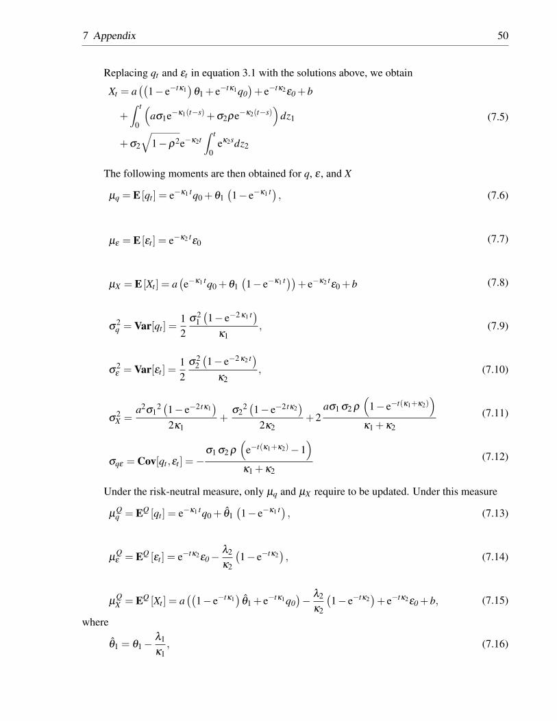
7 Appendix 50
Replacing qt and εt in equation 3.1 with the solutions above, we obtain
Xt = a((
1− e−tκ1)
θ1 + e−tκ1q0)+ e−tκ2ε0 +b
+∫ t
0
(aσ1e−κ1(t−s)+σ2ρe−κ2(t−s)
)dz1
+σ2
√1−ρ2e−κ2t
∫ t
0eκ2sdz2
(7.5)
The following moments are then obtained for q, ε , and X
µq = E [qt ] = e−κ1 tq0 +θ1(1− e−κ1 t) , (7.6)
µε = E [εt ] = e−κ2 tε0 (7.7)
µX = E [Xt ] = a(e−κ1 tq0 +θ1
(1− e−κ1 t))+ e−κ2 t
ε0 +b (7.8)
σ2q = Var[qt ] =
12
σ21(1− e−2κ1 t)
κ1, (7.9)
σ2ε = Var[εt ] =
12
σ22(1− e−2κ2 t)
κ2, (7.10)
σ2X =
a2σ12 (1− e−2 tκ1
)2κ1
+σ2
2 (1− e−2 tκ2)
2κ2+2
aσ1 σ2 ρ
(1− e−t(κ1+κ2)
)κ1 +κ2
(7.11)
σqε = Cov[qt ,εt ] =−σ1 σ2 ρ
(e−t(κ1+κ2)−1
)κ1 +κ2
(7.12)
Under the risk-neutral measure, only µq and µX require to be updated. Under this measure
µQq = EQ [qt ] = e−κ1 tq0 + θ1
(1− e−κ1 t) , (7.13)
µQε = EQ [εt ] = e−tκ2ε0−
λ2
κ2
(1− e−tκ2
), (7.14)
µQX = EQ [Xt ] = a
((1− e−tκ1
)θ1 + e−tκ1q0
)− λ2
κ2
(1− e−tκ2
)+ e−tκ2ε0 +b, (7.15)
where
θ1 = θ1−λ1
κ1, (7.16)
7 Appendix 51
7.2 Derivation of Futures Options Prices
7.3 Industrial Metals Consumption, Production, and Inventory
This appendix presents the global consumption, production, and inventory for industrial metals.
Inventory data is collected from major metal exchanges, the London Metal Exchange (LME), the
Commodity Exchange (COMEX), and the Shanghai Futures Exchanges (SHFE).

7 Appendix 52
(a) (b) (c)
(d) (e) (f)
(g) (h) (i)
(j) (k) (l)

7 Appendix 53
(m) (n) (o)
(p) (q) (r)
Figure 7.1: Plots of Consumption, Production, and Total Inventory for Industrial Metals.The total inventory is calculated as sum of available inventory at LME, COMEX, andShanghai Exchange.

7 Appendix 54
7.4 Industrial Metals Normalized Excess Supply and Deviation
from Mean
This appendix presents the normalized excess supply (q), the relationship between prices and "q",
and the deviations from the mean level for industrial metals.

7 Appendix 55
(a) (b) (c)
(d) (e) (f)
(g) (h) (i)
(j) (k) (l)
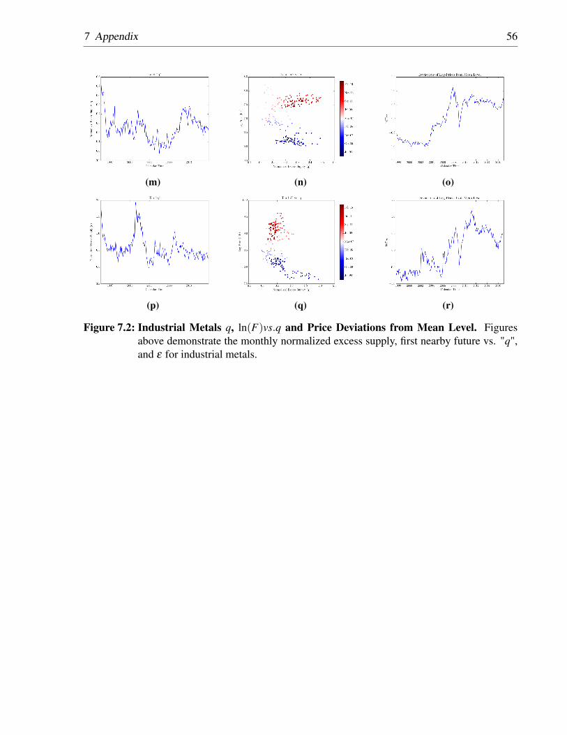
7 Appendix 56
(m) (n) (o)
(p) (q) (r)
Figure 7.2: Industrial Metals q, ln(F)vs.q and Price Deviations from Mean Level. Figuresabove demonstrate the monthly normalized excess supply, first nearby future vs. "q",and ε for industrial metals.

7 Appendix 57
7.5 Calibration
For the purpose of calibration, a Kalman filter process similar to that of Schwartz (1997) is utilized.
The two underlying stochastic factors in the proposed model are normalized excess supply, q, and
the deviation from mean level of log-prices, ε . Spot prices are unobservable for oil. Often, first
nearby futures’ prices are used as a proxy for the spot prices. Moreover, the published supply,
demand, and inventory data are only estimates of the true unobservable variables. This makes
straightforward calibration of the processes inaccurate. Hence, the model is put in a state-space
form to account for unknown true values of the state variables. The two state variables are the
q and ε . The Kalman filter is then applied to estimate the true value of the state variables’ time
series. The Kalman filter is an iterative prediction-correction algorithm. In each time step t, based
on the current estimate of parameters and state variables, the time t + 1 value of state variables
are estimated through a transition equation. The measurement variables are then estimated based
on the predicted state variables through the measurement equation. Finally, the predicted state
variables are corrected based on the prediction error, the difference between observed and predicted
data. The transition equation relating the state parameters at time t to the state parameters at time
t−∆t is set up as
x−t = At xt−∆t +Bt +wt (7.17)
where
x−t =
q−t
ε−t
, (7.18)
At =
e−κ1 t 0
0 e−κ2 t
, (7.19)
Bt =
θ1(1− e−κ1 t)
0
, (7.20)
7 Appendix 58
and wt is defined as transition noise with
E[wt ] = 02×2,Var[wt ] =
σ2q σqε
σ εq σ2ε
. (7.21)
Subsequently, the measurement equation relating the observables to state variables is set up
as
yt =Cτ x−t +Dt + vt , (7.22)
where
yt =
ln(F (t,τi))
qt
, (7.23)
Cτ =
a 1
1 0
, (7.24)
Dτ =
(rτi−δτi)τi
0
, (7.25)
and vt is defined as measurement noise with
E [vt ] = 0(n+1)×(n+1),Var [vt ] =
R1
. . .
Rn+1
, (7.26)
where Ri is measurement noise associated with ith observation.
Equations 7.17 to 7.26 set out the prediction stage of the Kalman filter. The correction stage
involves the following equations
P−t = AtPt−1A′t +Qt−1, (7.27)
Gt = P−t C′t
(CtP−t C
′t + vt
), (7.28)
xt = x−t +Gt(yt−Dt−Ct x−t
), (7.29)
and
Pt = (I−GtCt)P−t . (7.30)
7 Appendix 59
Finally, this iterative system is passed to an optimization engine to maximize the likelihood function
over the underlying parameters. The negative log-likelihood function is then derived asn+1
2T ln(2π)+
12 ∑
all tln(det(Vt))+ e
′tV−1
t et , (7.31)
where
Vt =CtP−t C′t + vt , (7.32)
and
et = yt−Dt−Ct x−t . (7.33)
Lastly, the maximum likelihood estimate of the parameters, the standard error of the parameters
and the optimal estimates of the state variables are obtained.
Top Related