


Languages
Pages
Legal


i
A NEW APPROACH FOR NON-INVASIVE CONTINUOUS
ARTERIAL BLOOD PRESSURE MEASUREMENT IN HUMAN
Thesis submitted for the degree of
Doctor of Philosophy
at the University of Leicester
by
Kong Yien Chin
Department of Cardiovascular Sciences
Medical Physics Group
University of Leicester
December 2010

ii
Kong Yien Chin
A New Approach for Non-Invasive Continuous Arterial Blood Pressure
Measurement in Human
Abstract
The need for continuous noninvasive arterial blood pressure (ABP) monitoring from an artery closer to the heart (i.e. the ascending aorta) has led to the research and
development work presented in this thesis. Clinical applications of continuous ABP
waveform include assessments of cardiac function, cerebral autoregulation, autonomic
function, arterial elasticity, physiological measurements in aerospace research, and also monitoring in anaesthesia and critical care.
The superficial temporal artery (STA) was chosen as the measurement site and the measurement technique was the arterial volume clamping with photoplethysmography
(PPG). The optoelectronic circuitry to measure PPG is contained in a specially designed
probe placed over the STA and kept in place with a lightweight aluminium head frame.
The complete prototype device (STAbp) also includes original designs for the pneumatic, electronic, signal processing, control and display sub-systems. A self-
calibration feature that regularly updates the PPG reference level (Setpt) was also
included to ensure accurate continuous ABP recording.
The performance of the STAbp was compared against the Finapres®. Five parameters
were evaluated: resting ABP (agreement, signal bandwidth, frequency response and
magnitude squared coherence, and assessment of drift) and ABP dynamic change
during isometric handgrip exercise. The agreement of resting ABP gave bias (SD) of -23.1 (15.05), -10.8 (13.83) and -12.4 (12.93) mmHg for systolic, mean (MAP) and
diastolic pressures respectively.
Further investigations were carried out to understand factors that can affect the accuracy of ABP measurements, notably the sensitivity of ABP to perturbation of the Setpt. Also,
differences between the external compressing pressure at the PPG peak pulsation
amplitude and the MAP were found to be normally distributed with mean (SD) of -4.7
(5.63) mmHg.
In conclusion, it is demonstrated that the new STAbp device has great potential as a new
tool for a wide range of clinical and research applications which require continuous
ABP waveforms.

iii
Acknowledgements
My deepest gratitude:
To the Department of Medical Physics led by Professor David Evans for giving me the
opportunity to pursue a PhD in this project.
To my supervisor Professor Ronney B. Panerai for his continuous patience, guidance
and support throughout the duration of my PhD studentship.
To Dr. Kevin Martin for his invaluable advice and support at the early stage of my PhD
studentship before his retirement.
To Mr. Graham Aucott, Mr. Glen Bush and Mr. Michael Squires from the electronic
and mechanical workshops for their ideas and support in providing the necessary test
equipments, and advice in the development of the prototype device.
To all volunteer subjects who have been supportive and endured the measurements for
this project.
To my line manager Dr. Christopher Degg for his ongoing encouragement and allowed
extra time off from my full time job while I was completing this thesis.
Finally, to so many more family members, friends and other colleagues who have been
kind and patient for me to progress with this project and to complete the thesis.

iv
CONTENTS
LIST OF FIGURES .......................................................................................................... vii
LIST OF TABLES ............................................................................................................. ix
LIST OF ABBREVIATIONS ............................................................................................ x
CHAPTER 1 INTRODUCTION.................................................................................. 1 1.1 Physiology of ABP Generation ................................................................................ 2
1.2 Rationale .................................................................................................................... 6
1.2.1 Continuous vs. Intermittent Measurements ........................................................... 6 1.2.2 Noninvasive vs. Invasive Measurements .............................................................. 7
1.2.3 Central vs. Peripheral Blood Pressure ................................................................... 8 1.2.4 State-of-the-Art CoNIBP Devices ........................................................................ 8
1.3 Applications of Continuous ABP Waveforms....................................................... 10
1.3.1 Anaesthesia and Critical Care ............................................................................. 10
1.3.2 Assessment of Cardiac Function ......................................................................... 11 1.3.3 Assessment of Arterial Elasticity ........................................................................ 11
1.3.4 Assessment of Autonomic Function ................................................................... 13 1.3.5 Assessment of Cerebral Autoregulation .............................................................. 14 1.3.6 Physiological Measurements in Aerospace Research .......................................... 15
1.4 Aims and Objectives ............................................................................................... 16
CHAPTER 2 BLOOD PRESSURE MEASUREMENT......................................... 17 2.1 Introduction.............................................................................................................. 17
2.2 The Evolution of ABP Measurement ..................................................................... 18
2.3 ABP Measurement Site ........................................................................................... 22
2.3.1 Selection of Alternative ABP Measurement Site ................................................. 22 2.3.2 Anatomy and Physiology of the STA ................................................................. 25
2.4 Classical ABP Measurement Techniques .............................................................. 31
2.4.1 Intravascular Measurements ............................................................................... 31 2.4.1.1 Catheter-tip type catheter ........................................................................... 32 2.4.1.2 Fluid-filled type catheter ............................................................................ 33
2.4.2 Sphygmomanometry .......................................................................................... 34
2.4.3 Oscillometry ...................................................................................................... 37 2.5 Techniques for CoNIBP Measurement .................................................................. 39
2.5.1 Applanation Tonometry ..................................................................................... 39 2.5.2 Volume Clamping Technique ............................................................................. 41
2.6 Potential Causes of Error in ABP Measurement ................................................... 44
2.7 Selection of a Suitable ABP Measurement Technique ......................................... 48 2.8 Conclusion ............................................................................................................... 50
CHAPTER 3 SYSTEM ARCHITECTURE ............................................................. 51 3.1 Introduction.............................................................................................................. 51
3.2 Design Criteria ......................................................................................................... 52 3.3 Instrumentation ........................................................................................................ 56
3.3.1 Probe ................................................................................................................. 56 3.3.2 Head Frame ....................................................................................................... 62
3.3.3 Regulated Compressing Pressure ........................................................................ 65 3.3.4 PPG Signal Generation....................................................................................... 68

v
3.3.5 Closed Loop Feedback Controller ...................................................................... 68 3.3.6 Mode Switch ...................................................................................................... 69 3.3.7 Operating Base and Software ............................................................................. 70
3.3.7.1 Open Loop Procedure ................................................................................ 71 3.3.7.2 Closed Loop Procedure .............................................................................. 73
3.4 Initial Assessments .................................................................................................. 77 3.4.1 Frequency Response Test ................................................................................... 77
3.4.2 Device Safety Evaluation ................................................................................... 79 3.5 Results ...................................................................................................................... 80
3.5.1 Open Loop Operation ......................................................................................... 80 3.5.2 Frequency Response........................................................................................... 80
3.5.3 Closed Loop Operation ...................................................................................... 83 3.6 Discussion ................................................................................................................ 85
3.7 Conclusion ............................................................................................................... 90
CHAPTER 4 PROTOTYPE DEVICE EVALUATION ........................................ 91 4.1 Introduction.............................................................................................................. 91 4.2 Data Analysis Techniques ...................................................................................... 93
4.2.1 Resting ABP: Agreement ................................................................................... 94 4.2.2 Resting ABP: Bandwidth ................................................................................... 94
4.2.3 Resting ABP: Frequency Response and Magnitude Squared Coherence .............. 97 4.2.4 Resting ABP: Assessment of Drift.................................................................... 100
4.2.5 ABP Dynamic Change during Activity ............................................................. 100 4.3 Comparative Study of two Finapreses................................................................. 103
4.3.1 Method ............................................................................................................ 103 4.3.2 Results ............................................................................................................. 106
4.3.2.1 Resting ABP: Agreement ......................................................................... 109 4.3.2.2 Resting ABP: Bandwidth ......................................................................... 121 4.3.2.3 Resting ABP: Frequency Response and Magnitude Squared Coherence ... 121 4.3.2.4 Resting ABP: Assessment of Drift ........................................................... 124 4.3.2.5 ABP Dynamic Change: Valsalva Manoeuvre ........................................... 124
4.4 Comparative Study of STAbp and Finapres ........................................................ 129 4.4.1 Method ............................................................................................................ 129
4.4.2 Results ............................................................................................................. 131 4.4.2.1 Resting ABP: Agreement ......................................................................... 135 4.4.2.2 Resting ABP: Bandwidth ......................................................................... 135 4.4.2.3 Resting ABP: Frequency Response and Magnitude Squared Coherence ... 137 4.4.2.4 Resting ABP: Assessment of Drift ........................................................... 137 4.4.2.5 ABP Dynamic Change: IHG Exercise ...................................................... 137
4.5 Inter-Study Comparisons ...................................................................................... 142
4.6 Discussion .............................................................................................................. 147 4.6.1 Recordings Excluded from Analysis ................................................................. 147
4.6.2 Main Findings .................................................................................................. 151 4.6.3 Potential Causes of Measurement Differences .................................................. 155
4.6.4 Limitations of Comparative Studies.................................................................. 157 4.6.5 Safety Evaluation ............................................................................................. 158
4.6.6 Suggestions for Future Work ............................................................................ 158 4.7 Conclusion ............................................................................................................. 160
CHAPTER 5 SENSITIVITY of ABP to PERTURBATION on Setpt ................ 161
5.1 Introduction............................................................................................................ 161 5.2 Method ................................................................................................................... 162

vi
5.2.1 Subjects and Measurements.............................................................................. 162 5.2.2 Protocols .......................................................................................................... 163 5.2.3 Data Analysis ................................................................................................... 163
5.3 Results .................................................................................................................... 165
5.3.1 Subjects ........................................................................................................... 165 5.3.2 Data Analysis ................................................................................................... 165
5.4 Discussion .............................................................................................................. 171 5.4.1 Main Findings .................................................................................................. 171
5.4.2 Implications from Findings .............................................................................. 172 5.4.3 Limitations of the Study ................................................................................... 172
5.4.4 Suggestions for Future Work ............................................................................ 173 5.5 Conclusion ............................................................................................................. 175
CHAPTER 6 PPG WAVEFORM ANALYSIS ...................................................... 176 6.1 Introduction............................................................................................................ 176 6.2 Method ................................................................................................................... 181
6.2.1 Subjects and Measurements.............................................................................. 181 6.2.2 Protocols .......................................................................................................... 182
6.2.3 Data Analysis ................................................................................................... 183 6.3 Results .................................................................................................................... 187
6.4 Discussion .............................................................................................................. 195
6.4.1 Main Findings .................................................................................................. 195 6.4.2 Previous Work ................................................................................................. 195
6.4.3 Implications from Findings .............................................................................. 196 6.4.4 Limitations of the Study ................................................................................... 197
6.4.5 Suggestions for Future Work ............................................................................ 198 6.5 Conclusion ............................................................................................................. 199
CHAPTER 7 CONCLUSIONS ................................................................................ 200 7.1 Review of Objectives ............................................................................................ 200
7.2 Original Contributions of Thesis .......................................................................... 202
7.3 Limitations of the Thesis ...................................................................................... 205
7.4 Suggestions for Future Work ................................................................................ 206 7.5 Conclusions............................................................................................................ 208
APPENDIX ELECTRONIC CIRCUITS DIAGRAMS ..................................... 209 Figure A.1 IRED Driver and Transimpedance Amplifiers .......................................... 209 Figure A.2 Piezo Valve with Regulated Compressed Air Supply ............................... 210
Figure A.3 Controller (for Regulated Compressing Pressure) ..................................... 211 Figure A.4 Pressure Transducer ................................................................................. 212
Figure A.5 PPG Signal Generation ............................................................................ 213 Figure A.6 Closed Loop Feedback Controller ............................................................ 214
Figure A.7 Mode Switch ........................................................................................... 215
BIBLIOGRAPHY ........................................................................................................... 216

vii
LIST OF FIGURES
Figure 1.1 A recording of a continuous ABP waveform. ................................................... 5
Figure 1.2 Variation of ABP waveforms in different arteries. ........................................... 5
Figure 2.1 Potential locations for CoNIBP measurement. .............................................. 23
Figure 2.2 The arterial network of the face and scalp. .................................................... 28
Figure 2.3 Tissue layers at the temporal region of the head............................................ 29
Figure 2.4 An adult STA imaged with MRI. ...................................................................... 30
Figure 3.1 Block diagram of the STAbp integrated prototype device. ............................ 57
Figure 3.2 The prototype design of the probe for the STAbp. .......................................... 61
Figure 3.3 Prototype design of the head frame for the STAbp......................................... 64
Figure 3.4 Block diagram of the regulated compressing pressure (G3). ........................ 66
Figure 3.5 Flowchart of the Open Loop Procedure (OLP).............................................. 72
Figure 3.6 Flowchart of the Closed Loop Procedure (CLP). .......................................... 75
Figure 3.7 Flowchart of the Setpt Self-Update subfunction. ............................................ 76
Figure 3.8 Experimental setup to evaluate frequency response of G3. ........................... 78
Figure 3.9 Recorded PPG waveform during Open Loop Procedure (OLP)................... 81
Figure 3.10 Frequency response curves of the regulated compressing pressure (G3). . 82
Figure 3.11 Resting ABP recording (STAbp vs. Finapres). ............................................. 84
Figure 3.12 ABP recording during Valsalva Manoeuvre (STAbp vs. Finapres). ........... 84
Figure 3.13 Possible placements of optoelectronic components relative to the STA. .... 88
Figure 4.1 Resting ABP waveforms (Finap2 vs. Finap1)............................................... 107
Figure 4.2 ABP waveforms during Valsalva manoeuvre (Finap2 vs. Finap1). ............ 108
Figure 4.3 Plots of means of ABP for „Finap‟ and „Test‟ main effects. ........................ 114
Figure 4.4 Plots of means of ABP for the „Finap x Test‟ interaction. ........................... 115
Figure 4.5a Test #1 plots of agreement in resting ABP (Finap2 vs. Finap1). .............. 116
Figure 4.5b Test #2 plots of agreement in resting ABP (Finap2 vs. Finap1). .............. 117
Figure 4.5c Test #3 plots of agreement in resting ABP (Finap2 vs. Finap1). .............. 118
Figure 4.5d Test #4 plots of agreement in resting ABP (Finap2 vs. Finap1). .............. 119
Figure 4.6 Plots of means of bandwidth limits for ABP pulses...................................... 122
Figure 4.7 Spectral curves between ABP measurements with two Finapreses. ........... 123
Figure 4.8 Plots of means of percentage change in the assessment of ABP drift. ........ 125
Figure 4.9 Assessment of drift in resting ABP (Finap2 vs. Finap1). ............................. 126
Figure 4.10 Plots of means of ABP percentage change during Valsalva manoeuvre. . 127
viii
Figure 4.11 ABP dynamic change during Valsalva manoeuvre (Finap2 vs. Finap1).. 128
Figure 4.12 Resting ABP waveforms (STAbp vs. Finap1). ............................................ 133
Figure 4.13 SBP, MAP and DBP during IHG exercise. ................................................. 134
Figure 4.14 Plots of agreement in resting ABP (STAbp vs. Finap1). ............................ 136
Figure 4.15 Spectral characteristic curves (STAbp vs. Finap1). ................................... 139
Figure 4.16 Assessment of drift in resting ABP (STAbp vs. Finap1). ............................ 140
Figure 4.17 ABP dynamic change during IHG exercise (STAbp vs. Finap1)............... 141
Figure 4.18 Comparison of spectral responses between both studies. .......................... 146
Figure 4.19 PPG with fairly constant baseline. .............................................................. 150
Figure 4.20 Atypical vs. typical PPG waveforms. .......................................................... 150
Figure 5.1 ABP waveform after a ΔV perturbation on the Setpt in STAbp. .................. 166
Figure 5.2 Sample distribution curves for SE and SP. ..................................................... 168
Figure 5.3 Sample distribution curves for STA and F . ............................................... 169
Figure 5.4 Sample distribution curves for absolute values |SE|, |SP| and | STA |. ......... 170
Figure 6.1 Simultaneous recording of the compressing pressure and the PPG. .......... 178
Figure 6.2 Example computation of PdiffA from the GaPP ˆ curve. ................................ 186
Figure 6.3 RMSE of the polynomial curve fitting of aPPG arrays. .............................. 188
Figure 6.4 Computation of PdiffA from the GaPP ˆ curve................................................ 189
Figure 6.5 Histogram for the sample distribution of PdiffA. ............................................ 193
Figure 6.6 Relationship of intra-subject PdiffA with age. ................................................ 194

ix
LIST OF TABLES
Table 2.1 Potential causes of error in noninvasive ABP measurement........................... 45
Table 3.1 Explanation of labels in Figure 3.1. .................................................................. 58
Table 4.1 Twelve possible combinations of two Finapreses and two fingers. .............. 104
Table 4.2 ANOVA p-values for SBP (two Finapreses with four tests). ......................... 111
Table 4.3 ANOVA p-values for MAP (two Finapreses with four tests). ........................ 112
Table 4.4 ANOVA p-values for DBP (two Finapreses with four tests).......................... 113
Table 4.5 Bias (SD) in resting ABP (Finap2 vs. Finap1). .............................................. 120
Table 4.6 Mean (SD) of RMSE in resting ABP (Finap2 vs. Finap1). ............................ 120
Table 4.7 ANOVA p-values for the 95% and 99% bandwidth limits. ............................ 122
Table 4.8 ANOVA p-values for the assessment of drift................................................... 125
Table 4.9 ANOVA p-values for VM during Valsalva manoeuvre. ............................ 127
Table 4.10 Summary of results from both comparative studies. .................................... 144
Table 4.10 Summary of results from both comparative studies (continued). ................ 145
Table 4.11 Further comparison between both comparative studies. ............................. 145
Table 5.1 Computation results of SE, SP, STA and F . ................................................. 166
Table 6.1 Relationship between pulsation amplitude and intra-arterial MAP. ............ 179
Table 6.2 Individual results of PdiffA from five subjects. ................................................. 192

x
LIST OF ABBREVIATIONS
First used in
Chapter
ABP Arterial blood pressure 1
ANOVA Analysis of variance 4
BRS Baroreceptor reflex sensitivity 1
CBF Cerebral blood flow 1
CLP Closed Loop Procedure 3
CoNIBP Continuous noninvasive ABP 1
DBP Diastolic blood pressure 4
DFT Discrete Fourier transform 4
FFT Fast Fourier transform 4
Finap1 Finapres #1 (reference device) 4
Finap2 Finapres #2 (test device) 4
IHG Isometric handgrip 4
IRED Infrared emitting diode 3
MAP Mean arterial pressure 4
MRI Magnetic resonance imaging 2
n Sample size 4
OLP Open Loop Procedure 3
PD Photodetector 3
PPG Photoplethysmogram 2
RMSE Root mean squared error 4
SBP Systolic blood pressure 4
SD Standard deviation 2
Setpt PPG reference value used in STAbp 3
STA Superficial temporal artery 2
STAbp Prototype device to monitor ABP in the STA 1

1
CHAPTER 1 INTRODUCTION
Overview
The history of arterial blood pressure (ABP) measurement was documented as early as
1628 by William Harvey when he described the existence of blood circulation in his
book De Motu Cordis. Today, ABP measurement plays an essential role in healthcare
establishments such as clinics, operation theatres, hospital wards, and accident and
emergency departments. Its relevance expands from providing an initial clinical
assessment for hypertension or hypotension, continuous ABP monitoring in operation
theatres and critical care, to contributing as an important parameter in a wide range of
physiological research.
Chapter Outline
This chapter will set the scene regarding ABP measurements that became the driving
force for the research work presented in this thesis. In the following section 1.1, the
physiology of ABP generation is first described. Section 1.2 will then describe the
rationale of the research in more detail regarding the importance of continuous and
noninvasive as opposed to single, intermittent, or invasive ABP measurement
modalities. The importance of monitoring ABP from an artery close to the heart will
also be emphasized. Section 1.3 describes the applications, whether clinical or in
research, that require continuous ABP waveforms. The aim and objectives of this thesis
will then be established in section 1.4. Finally, the outline of subsequent chapters will
be presented, the contents of which will demonstrate its contributions towards the
advancement in the field of continuous noninvasive ABP (CoNIBP) measurements.

2
1.1 Physiology of ABP Generation
The human cardiovascular system is a closed network of blood vessels. ABP generation
starts with left ventricular contraction and it propagates from the ascending aorta to
other arteries, arterioles and capillaries. The changes in ABP during cyclical pumping of
the heart generate a pressure wave that reaches a maximum and then a minimum in each
cardiac cycle, known as the systolic and diastolic pressures respectively. Figure 1.1
shows an example where a continuous ABP waveform is recorded.
A complex regulatory system of inter-related mechanisms is involved to ensure
sufficient blood flow reaches the tissues and vital organs. They are broadly categorised
as short-, intermediate- and long- term ABP regulatory mechanisms (Guyton and Hall,
1997). The short-term ABP change is mainly regulated by the baroreceptor feedback,
central nervous system response to ischaemia and chemoreceptor mechanisms. These
also include local myogenic and metabolic mechanisms, and central sympathetic control
of peripheral resistance to ensure adequate blood flow supply through the vascular
network (Levy and Pappano, 2007). These mechanisms react within seconds to return
the ABP level back to normal. During this process, there may be changes in vasomotor
tone (i.e. vasoconstriction or vasodilation), heart rate, heart contractility and cardiac
output.
The intermediate-term pressure regulatory mechanisms are activated a few minutes after
an acute ABP change. These involve the renin-angiotensin vasoconstrictor mechanism,
stress-relaxation of the vasculature and fluid shift through capillary walls. When the
ABP decreases, angiotensin activates vasoconstriction in the arterioles which raises the

3
blood pressure. It also causes water and salt retention in the blood through the kidneys.
Lastly, the long-term blood flow is further regulated by the kidneys through the renal-
blood volume pressure control mechanism. It usually takes at least a few hours to show
significant response. Angiotensin causes the secretion of aldosterone in the adrenal
glands which increases water and salt re-absorption by the kidney tubules. The
interaction of the renin-angiotensin mechanism with aldosterone regulates the water and
salt retention in the body fluid until the ABP is returned to normal.
Along the vessel pathway, the pressure wave is changed. This is due to a combination of
the expansion-recoil effect of the elastic vessel wall, vasomotor tone and peripheral
resistance (Thibodeau and Patton, 2002). These lead to different intensity and timing of
pulse wave propagation (forward flow) and wave reflection (backward flow) along the
pathway (Avolio, 1992; Belardinelli and Cavalcanti, 1992; O'Rourke et al., 2003;
O'Rourke and Yaginuma, 1984; Westerhof et al., 2006). The propagating wave from the
ascending aorta overlaps with the reflected wave from the periphery. The central ABP
waveform is hence the summation of the cyclical pressure, the propagated and the
reflected pressure waves. This phenomenon also applies to the ABP along the rest of the
arterial tree and results in different ABP waveshapes in different arteries.
In comparison with ascending aortic pressure, peripheral ABP waveforms in young
individuals with more elastic vessel walls tend to produce delayed and increased
systolic peak, steeper ejection gradient to systolic peak and a slightly lower diastolic
value with more distinct trough. In addition to this, there is a small drop in mean
pressure due to a pressure gradient in smaller arteries (Avolio, 1992; Karamanoglu et
al., 1993; O'Rourke, 1992; O'Rourke et al., 2003; O'Rourke and Yaginuma, 1984;

4
Westerhof et al., 2006). As the arterial wall stiffens with age, vessel resistance is
increased. This usually leads to a raised mean ABP in the elderly. The pulse wave
travels faster due to the stiffer vessel walls, with reflected wave returning quicker
towards the aorta. This further raises the systolic pressure close to the heart (i.e.
ascending aorta) (Levy and Pappano, 2007). In all age groups, local regulation of blood
flow at the periphery with strong sympathetic innervation may further distort the ABP
waveforms (Wesseling et al., 1995). Figure 1.2 shows an illustration of ABP waveforms
measured from the ascending aorta to the femoral artery in three adult humans
(O'Rourke and Nichols, 2005). Consequently, the site of ABP measurement needs to be
selected appropriately with reference to the pathology and clinical queries.

5
Figure 1.1 A recording of a continuous ABP waveform.
The instantaneous change of the ABP is recorded. In each cardiac cycle (indicated as
„c‟), the systolic („s‟), mean („m‟) and diastolic („d‟) pressures can be computed.
Figure 1.2 Variation of ABP waveforms in different arteries.
ABP waveforms measured along the arterial pathway from the ascending aorta to the
femoral artery in three adult humans aged 24, 54 and 68 years. In the oldest subject, there is little amplification in the pressure wave; whereas, in the youngest subject, the
amplitude of the pressure pulse wave is increased towards the periphery (image
adapted from O'Rourke and Nichols (2005)).
‘c’ ‘c’ ‘c’ ‘c’ ‘c’
„s‟
„d‟
„m‟

6
1.2 Rationale
In clinical and research practice, there is still a lack of suitable CoNIBP monitoring
devices that can suit different needs. Ideally, such devices should monitor the ABP from
an artery close to the heart, i.e. the ascending aorta. The availability of such devices will
not only encourage its use in clinical areas, it will also increase research endeavours that
particularly require continuous recording of the ABP waveform. This will potentially
further generate new knowledge in the field of physiological measurements. Three main
characteristics of ABP measurement devices should be considered and they are
described in the subsections below.
1.2.1 Continuous vs. Intermittent Measurements
ABP measurement is often performed using single or intermittent measurements of
systolic, mean, and diastolic pressures to detect hypertension or hypotension. The
frequency of the measurements will depend on clinical needs or specific research
protocol. In single or intermittent measurements, beat-to-beat changes of ABP are not
available.
In continuous measurements, on the other hand, an instantaneous ABP change is
recorded. Close observation of continuous ABP measurements is essential in many
clinical or research applications where additional information can be extracted from the
ABP waveform or where values of systolic, mean and diastolic pressures are required
for all heart beats during a given period of time.

7
1.2.2 Noninvasive vs. Invasive Measurements
Historically, before the advent of CoNIBP measurement techniques, the clinical
assessments of ABP were based on invasive measurements. Although the invasive
measurement method is used as the ‘gold standard’, it carries a high risk of infection
and other clinical complications (Carroll, 1988; Murray, 1981; Prian, 1977; Toll, 1984;
West et al., 1991). These include haemorrhage (Pierson and Hudson, 1983), arrhythmia
and ischaemia (Murray, 1981; Puri et al., 1980), local skin discolouration, bruising and
haematoma, neurological damage (Bull et al., 1980; Luce et al., 1976), embolism and
thrombosis (Bedford, 1978; Downs et al., 1974; Evans and Kerr, 1975; Jones et al.,
1981; Prian et al., 1978), and arterial vasospasm (Kurki et al., 1987; Smith et al., 1985).
Two main types of intravascular catheters will be described later in section 2.4.1. They
are the fluid-filled type and the catheter-tip type catheters. They are designed for single
use only. The catheter-tip type catheter is much more expensive, often in excess of £400
each. In addition to that, the procedure is a specialised skill and hence it can only be
carried out by a trained person.
A noninvasive device does not normally require disposable parts and the measurement
process is easily repeatable. It is usually a much less expensive alternative in the long
run. The risk of infection and other complications that are common in invasive
measurement techniques are negligible. Patients can leave the clinic or continue with
their daily lives immediately after a noninvasive ABP measurement procedure is
completed. These same benefits also apply to research studies. More studies can hence
be carried out with less ethical issues involved.

8
1.2.3 Central vs. Peripheral Blood Pressure
As described in section 1.1, the ABP waveform varies dependent on the measurement
site (Figure 1.2). The ABP waveforms in different arteries are influenced by the pulse
wave propagation and reflection (Avolio, 1992; O'Rourke, 1992; O'Rourke et al., 2003;
O'Rourke and Yaginuma, 1984). Local regulation of blood flow further affects the
agreement between the central (i.e. ascending aorta) and peripheral ABP. Assessments
based on peripheral ABP waveforms, for instance, measured with the Finapres, may
hence lead to misdiagnosis and/or inadequate treatment (Williams et al., 2006).
1.2.4 State-of-the-Art CoNIBP Devices
The three previous sections provide brief justification for the need of devices that can
perform continuous noninvasive measurements of ABP close to the heart. Not
surprisingly, there are already several CoNIBP measurement devices currently in the
market. These devices include the Finapres® (superseded by Portapres® and
Finometer®), SphygmoCor®, Colin®, and Millar® Mikrotip®. Finapres measures the
ABP from the digital (finger) artery (Imholz et al., 1998; Maestri et al., 2005; Schmidt
et al., 1992); SphygmoCor tonometer measures the pulse waveform from the radial and
carotid arteries; Colin tonometer from the radial artery (Birch and Morris, 2003; Zion et
al., 2003), and Millar micromanometer-tipped tonometric probe from the radial and
carotid arteries (Chen et al., 1995; Kelly et al., 1989).
The availability of such devices gave considerable impetus to many laboratory based
applications, but for several reasons they do not cover all the clinical and research needs
for CoNIBP measurement. For instance, carotid ABP should not be measured

9
continuously as this may interrupt its blood supply to the head, especially the brain.
Similarly, the finger ABP cannot be reliably monitored in some patient groups, namely,
premature neonates due to small and vulnerable digits, patients with lower arm diseases,
e.g. Raynaud’s disease and arthritis (Nelesen and Dimsdale, 2002; Panerai et al., 2006),
and patients with lower arm burns or amputees. Other devices like SphygmoCor, Colin
and Millar are not self-calibrating and can lead to significant errors in long term
recordings. The self-calibration feature will be explained in more detail in section 2.5.
In summary, despite the availability of different types of CoNIBP devices that meet
some of the needs for continuous ABP monitoring, there are still limitations and unmet
needs which justify the search for alternative approaches. Within this broad remit, the
following sections review the wide field of ABP applications, which will provide the
basis for a detailed proposal in section 1.4.

10
1.3 Applications of Continuous ABP Waveforms
The applications of continuous ABP waveform encompass the areas of anaesthesia and
critical care, cardiac function, arterial elasticity, autonomic function, cerebral
autoregulation and space research. As mentioned in previous sections, the use of a
noninvasive measurement device would always be preferred although currently this
option is not always available.
1.3.1 Anaesthesia and Critical Care
ABP monitoring is mandatory during anaesthesia, but the need for continuous
measurement is usually restricted to cardiac surgery and other critical conditions where
there is a risk of rapid cardiovascular deterioration (Hutton and Prys-Roberts, 1994;
Kemmotsu et al., 1991b).
Continuous ABP monitoring in very ill patients ensures that the patient’s blood pressure
is stable during recovery or following administration of medications (Andriessen et al.,
2004; Rolfe et al., 1987). This applies especially to patients in critical care such as the
coronary and neonatal intensive care units. Continuous ABP monitoring in coronary
care is particularly relevant to assess patients’ cardiac function before, during or after
heart surgery (Hirai et al., 2005; Pinna et al., 2000; West et al., 1991). Any abnormal or
sudden blood pressure change can be rapidly detected and hence immediate action can
be taken (Hughes et al., 1994; Hutton, 1994).

11
1.3.2 Assessment of Cardiac Function
Combined with other clinical measurements, continuous ABP waveform recording
provides additional information in the evaluation of cardiac and coronary
haemodynamics to identify abnormal conditions such as congenital heart disease,
dysrhythmias, pulsus alternans (Euler, 1999), stenosis (Nichols and O'Rourke, 2005)
and valve dysfunction (Levin, 1972; Murgo et al., 1980). The evaluation is also useful
to minimise risks such as atrial fibrillation, left ventricular hypertrophy, cardiac failure
or sudden death (O'Rourke and Brunner, 1992).
Several parameters can be derived from the continuous ABP waveform in the
assessment of cardiac function. These include aortic input impedance (Murgo et al.,
1980), cardiac output (Jansen et al., 2001), systolic time intervals (Weissler et al.,
1968), myocardial contractility (Brown and MacGregor, 1982) and left ventricular
ejection time (Gerhardt et al., 2000). In comparison with healthy subjects, these
parameters were altered in patients with cardiac pathology (Ferro et al., 1995; Martin et
al., 1974; Nichols and O'Rourke, 2005; Takazawa et al., 1998; Weissler et al., 1968).
1.3.3 Assessment of Arterial Elasticity
With advancing age or pathology, progressive changes in the collagen and elastic
content of the arterial wall (Levy and Pappano, 2007) can lead to reductions in arterial
elasticity. Different terminologies have been used in this field, i.e. compliance,
distensibility and stiffness (O'Rourke and Nichols, 2005). With reduced arterial
elasticity, changes in ABP waveshape can be detected and used to quantify the extent of

12
arterial wall damage (Lehmann et al., 1992; Lopez-Beltran et al., 1998; Sollers, III et
al., 2006).
Reduced arterial elasticity is considered a risk factor for cardiac failure, myocardial
infarction and stroke (O'Rourke and Nichols, 2005). The arterial elasticity is quantified
by a range of indices. These include the augmentation index, pulse wave velocity,
arterial distensibility, arterial compliance, pulse pressure, diastolic decay and
characteristic impedance (O'Rourke and Brunner, 1992; O'Rourke and Nichols, 2005;
Stergiopulos et al., 1999; Tanaka et al., 2002). The computation of these indices
requires the use of continuous ABP waveform, although only a small number of cardiac
cycles is usually sufficient.
As examples, increases in augmentation index and pulse wave velocity have shown
associations with cardiovascular disease (e.g. atherosclerosis, ischaemic heart disease,
left ventricular hypertrophy and coronary disease) (Avolio et al., 1985; Cockcroft and
Wilkinson, 2002; Millasseau et al., 2002; Nurnberger et al., 2002; Roman et al., 1995;
Saba et al., 1993; Sollers, III et al., 2006; Vaitkevicius et al., 1993), diabetes,
hypertension (Davies and Struthers, 2003; Meaume et al., 2001; Stergiopulos et al.,
1999), end stage renal disease (London et al., 2001), and an increase in mortality and
morbidity from coronary heart disease in the elderly (Lind et al., 2004; Sugawara et al.,
2007).

13
1.3.4 Assessment of Autonomic Function
Within its many functions, the autonomic nervous system plays a major role in the short
term control and regulation of ABP. The ABP is constantly monitored by baroreceptors
located primarily in the carotid sinus and aortic arch, but to a lesser extent in the walls
of arteries, veins and right atrium (Marieb, 2004). A change in ABP triggers impulses
firing from the baroreceptors, which are transmitted to the cardioregulatory centre of the
central nervous system in the medulla oblongata. From the cardioregulatory centre,
efferent impulses are conducted by the vagus and sympathetic nerves to regulate the
blood pressure back to the normal level by changes in heart rate, left ventricular
contractility and peripheral resistance (Guyton and Hall, 1997).
The effectiveness of the short term ABP regulation can be assessed by the parameter
known as the baroreceptor reflex sensitivity (BRS) (Dawson et al., 1997; Lucini et al.,
1994; Persson et al., 2001; Smyth et al., 1969). BRS is expressed by the change in
cardiac cycle duration for a given change in systolic ABP (units of ms/mmHg). BRS
can be computed in the time or frequency domain (Dawson et al., 1997; Frattola et al.,
1997; Persson et al., 2001; Smith et al., 2008). Analysis in either domain requires the
use of a continuous ABP waveform (Pinna et al., 2000).
While studies showed that there is generally a progressive decline of BRS with
advancing age in healthy subjects (Dawson et al., 1999b; James et al., 1996; O'Brien et
al., 1986), a decline of the BRS is also reported in pathological conditions such as heart
failure, myocardial infarction (Persson et al., 2001), ischaemic stroke (Atkins et al.,
2010; Eveson et al., 2005), cerebrovascular disease or injuries (Baguley et al., 2008;
Johnson et al., 2006), diabetes (Ewing et al., 1985; Weston et al., 1996b), renal failure,

14
traumatic quadriplegia (Omboni et al., 1996), abnormal left ventricular function, pre-
eclampsia during pregnancy (Rang et al., 2002), hypertension (Sleight, 1991),
alcoholism (Kollensperger et al., 2007), Parkinson’s disease (Goldstein et al., 2002;
Parati et al., 1995), syncope (Krediet et al., 2005; van Lieshout et al., 2003), orthostatic
intolerance (Imholz et al., 1990; Swenne et al., 1995; ten Harkel et al., 1992) and pure
autonomic failure (Goldstein et al., 2002; Omboni et al., 1996; Rang et al., 2002).
1.3.5 Assessment of Cerebral Autoregulation
Cerebral blood flow (CBF) autoregulation is a homeostatic mechanism that maintains
the mean CBF (or CBF velocity) relatively constant despite changes in cerebral
perfusion pressure (Panerai, 1998). Impaired cerebral autoregulation was found in
several conditions, e.g. hypercapnia (Birch et al., 1995; Dineen et al., 2010), carotid
artery disease (Hu et al., 1999; Panerai, 2008; Reinhard et al., 2004), middle cerebral
artery stenosis (Dawson et al., 1999a; Haubrich et al., 2003), severe head injury and
subarachnoid haemorrhage (Panerai, 2008), prematurity of the newborn (Panerai et al.,
1998) and stroke (Atkins et al., 2010; Dawson et al., 2003).
Continuous ABP waveform is needed in the assessment of dynamic cerebral
autoregulation (Dineen et al., 2010; Panerai et al., 1999; Sammons et al., 2007). The
transient change in the CBF (or CBF velocity) following a rapid change in the ABP can
be analysed (Aaslid et al., 1989). CBF is usually monitored using the transcranial
Doppler ultrasound technique. The ABP waveform (as input) is analysed in the
frequency domain by computing a transfer function in relation to the CBF (as output).

15
For example, a reduced phase response indicates an impairment of the cerebral
autoregulation (Panerai, 2008).
1.3.6 Physiological Measurements in Aerospace Research
With the expansion of space exploration, the assessment of cardiovascular physiology
in space travel continues to play a crucial role to monitor the cardiovascular health of
astronauts (Karemaker, 1995; Krol and Simons, 1995). Astronauts have been found to
experience short term orthostatic intolerance, impaired exercise performance and other
changes in their cardiovascular health after returning to earth from a long stay in space
with zero gravity. To study these alterations, continuous recording of ABP waveform
has been seen as essential (Hughson, 2009; Sigaudo-Roussel et al., 2002).

16
1.4 Aims and Objectives
Aims
The previous sections highlighted the increasing importance of CoNIBP monitoring for
specialised clinical applications and research work. Although considerable progress has
been achieved with existing devices, further work in this area is needed to explore the
possibility of performing measurement at alternative sites, for example closer to the
heart as compared to the finger. Also of considerable importance is to develop in-house
expertise to allow future developments that could benefit industry in the United
Kingdom.
Objectives
To achieve the aims above, specific objectives would be:
i. To identify suitable site of measurement with appropriate measurement technique;
ii. To design and develop a prototype device;
iii. To perform preliminary evaluation of the prototype device.
Thesis Outline
The following chapters will first begin with an overview of the evolution of ABP
measurements, measurement techniques and site of measurement (chapter 2). This will
be followed by the detailed description of a new CoNIBP monitoring prototype device
known as the STAbp (chapter 3). Chapter 4 will evaluate the STAbp device against the
Finapres, a commercial CoNIBP monitoring device. Further investigations relevant to
the STAbp device are presented in chapters 5 and 6. These chapters address possible
refinements for future improvements of the prototype device. Finally, chapter 7 will
present the conclusions and suggestions for further work.

17
CHAPTER 2 BLOOD PRESSURE MEASUREMENT
2.1 Introduction
Chapter 1 presented the rationale of the thesis, which is the need for a CoNIBP
monitoring device measured from an artery closer to the heart. The applications of
continuous ABP waveform in a wide range of physiological assessments and research
encourage the use of a noninvasive technique rather than invasive measurements that
carry a significant risk of infection and other clinical complications, and also has cost
implications. The outcome of these applications shows the potential to provide
clinicians with additional information to treat and manage illnesses more effectively.
The objectives of this chapter are:
i. To give an overview of the evolution of ABP measurement (section 2.2);
ii. To present the selection process for an alternative ABP measurement site closer to
the heart, followed by the anatomy and physiology of the selected site (section 2.3);
iii. To give an overview of the classical ABP measurement techniques and the
techniques for CoNIBP measurement (sections 2.4 and 2.5);
iv. To identify potential causes of error in noninvasive ABP measurement techniques
(section 2.6);
v. To present the selection process and decide on a suitable technique for CoNIBP
monitoring (section 2.7).

18
2.2 The Evolution of ABP Measurement
The history of blood pressure measurement can be traced back to William Harvey when
he described the existence of blood circulation in his book De Motu Cordis in 1628
(Hutton and Clutton-Brock, 1994; Paskalev et al., 2005; Wesseling, 1995). About a
century later, Reverend Stephen Hales (1733) first measured blood pressure directly
from the femoral and carotid arteries of non-anaesthetised horses by inserting a long
glass tube upright into an incision on a horse’s artery. Blood pressure was estimated by
monitoring the change in height of the blood level in the tube as the heart pumped
cyclically.
In 1826, Jean Poiseuille constructed a more convenient mercury column manometer,
and the millimetre of mercury (mmHg) was used as the unit of measurement.
Approximately two decades later, Carl Ludwig successfully recorded invasive
continuous blood pressure in animals graphically inscribed on a slowly rotating sooted
drum, called the kymograph. Jean Faivre later (1856) demonstrated the direct intra-
arterial pressure measurement in man and used the mercury column to establish the
mean blood pressure. His measurements focused on the humeral and femoral arteries.
In 1858, Étienne-Jules Marey measured the blood pressure in the forearm with a sealed
water-filled chamber. As the pressure in the chamber was raised, its pressure was
monitored with a mercury column manometer. The blood pressure pulsation was
simultaneously recorded graphically on a polygraph. Marey observed that the blood
pressure showed a change of oscillation amplitude as the water pressure was increased,
forming an approximately bell-shape amplitude curve. It was later considered by

19
Angelo Mosso in 1895 that at maximum oscillation, the internal and external pressures
were equal (Hutton and Clutton-Brock, 1994).
The concept of systolic and diastolic pressures began to unfold when Samuel von Basch
recorded the first noninvasive measurement of systolic blood pressure in 1880 from the
radial artery of a patient (Paskalev et al., 2005). Towards the end of the 19th century,
Scipione Riva-Rocci invented an inflatable upper arm rubber cuff to obstruct the blood
flow of the brachial artery. A mercury column was used to measure the pressure
required to inflate the arm cuff until the pulse distal to the cuff became impalpable.
During cuff deflation, when the pulse distal to the cuff reappears, it was identified as the
systolic pressure (Paskalev et al., 2005; Riva-Rocci, 1896). However, determining the
diastolic pressure remained an unresolved issue at the time. Furthermore, although
revolutionary, his cuff was too narrow, resulting in inaccurate measurements. Heinrich
von Recklinghausen (1901) later recognised this error and widened the cuff from 5 to
13 cm. At about the same time, Nikolai Korotkoff (1905) described the auscultatory
sounds heard with a stethoscope placed over the brachial artery below an encircling
upper arm cuff during gradual deflation. The five phases of Korotkoff sounds were later
described by Edward Goodman and Alexander Howell in 1911 to determine the systolic
and diastolic pressures (Hutton and Clutton-Brock, 1994). The measurement protocol
which has now become standard was recommended by Joseph Erlanger (1916a).
By 1933, Bertel von Bonsdorff had developed a monitoring system that compared the
finger blood pressure with the intra-arterial pressure near the elbow. He emphasised the
importance of appropriate frequency response in measurement devices to reproduce the
blood pressure pulsations faithfully.

20
The need for measuring the ABP more frequently throughout the day was gradually
recognised due to changes in blood pressure. The phenomenon of white coat
hypertension further encouraged intermittent measurements of ABP throughout the day
to assess its variation. White coat hypertension is a temporarily raised ABP in patients
due to anxiety in a clinical environment (Celis and Fagard, 2004; Pickering et al., 1988).
With the need for intermittent measurements, automated noninvasive ABP
measurement devices began to emerge. Numerous models became available both for
home and clinical use. Such devices gained popularity due to their ease of use and
negligible risk of infection, in addition to their low cost and high reusability. This
development facilitated ambulatory ABP monitoring which provides a profile of the
patient's blood pressure in conditions that are more representative of the patient's
lifestyle.
Continuous recording of ABP waveform continues to play an important role clinically.
The risk of infection and other clinical complications, and cost implications have
motivated the development of noninvasive approaches for recording instantaneous
variation of ABP. The development of CoNIBP monitoring using the volume clamping
technique was pioneered by Jan Penaz in 1967 (Penaz, 1973), and the importance and
potential of his contribution was increasingly recognised by researchers and clinicians
in the 1980s. Taking full advantage of microprocessors, software programming,
pneumatics, optoelectronics and feedback control mechanisms, a measurement device
using this technique automatically monitors the finger ABP continuously. Penaz’s
invention was later developed commercially and marketed as Finapres® by the Ohmeda
Company (Imholz et al., 1993; Langewouters et al., 1998; Wesseling, 1995). At about

21
the same time, a similar research led by Ken-ichi Yamakoshi from Japan had also
developed a finger ABP monitoring device based on Penaz’s technique and several
notable papers were published (Kawarada et al., 1991; Nakagawara and Yamakoshi,
2000; Tanaka and Yamakoshi, 1996; Yamakoshi et al., 1983; 1988; 1980). Finapres
was later superseded by the Portapres® and Finometer® which also monitor the finger
ABP. With regards to the Japanese group, their many contributions were not followed
by further communications, evaluative studies or industrial developments, which
included the ABP measurements from the finger and superficial temporal arteries.
The development of CoNIBP monitoring devices opened up new research interests for a
wide range of clinical applications due to the additional information that can be
extracted from continuous ABP waveforms (section 1.3). On the other hand, the need
for measurement of ABP at a more central site is still a challenge.

22
2.3 ABP Measurement Site
The second objective set out in section 2.1 is to select an alternative ABP measurement
site closer to the heart suitable for CoNIBP monitoring. The following subsection
describes the selection process, from which a decision for the measurement site is made.
This is then followed by a more detailed description of its anatomy and physiology.
2.3.1 Selection of Alternative ABP Measurement Site
To begin from a general perspective, an alternative ABP measurement site should meet
the following desirable criteria:
i. Proximity to the heart;
ii. Prolonged compression without causing irreversible physiological damage, such as
ischaemia, necrosis or bleeding;
iii. Ease and convenience of locating the arterial pulsation through palpation;
iv. Possibility of compressing the artery by external means;
v. Variation of the arterial pulse can be measured with current sensor technology;
vi. Low sensitivity to temperature change in the surrounding.
Figure 2.1 shows the possible measurement sites for CoNIBP monitoring (Hall, 2001;
Marieb, 2004). Criteria (i) and (ii) are the dominant factors. Any measurement site that
fails to meet these two criteria was excluded before the other criteria were considered.

23
Figure 2.1 Potential locations for CoNIBP measurement.
(Image adapted from Hall (2001)).
Tragus
Supraorbital artery

24
Starting with criterion (i), arteries shown in Figure 2.1 further away from the heart than
the radial artery were first excluded. Therefore, the remaining arteries are the tragus of
the ear, the brachial, common carotid, facial, supraorbital, superficial temporal and
femoral arteries. Next, three of these remaining arteries were considered not suitable to
meet criterion (ii). They are the common carotid, brachial and femoral arteries. The
common carotid artery supplies blood to the head intra- and extra- cranially, any
prolonged compression could cause severe cerebral damage. For the brachial artery,
prolonged compression could lead to venous congestion or ischaemia in the forearm,
wrist and the hand (Boehmer, 1987; Dorlas et al., 1985; Gravenstein et al., 1985; van
Egmond et al., 1985; Wesseling et al., 1985). For the femoral artery, due to its location
near the groin, privacy is a concern and prolonged compression would impair blood
circulation in the lower limb.
From this exclusion process, there are only four measurement sites to be considered
further, i.e. the tragus of the ear, facial, supraorbital and superficial temporal arteries.
These arteries are superficially located in the skin tissue. This means that criteria (iv)
and (v) can be met. To locate these four arteries through palpation (criterion (iii)), it is
very much trial and error for the artery in the tragus of the ear, supraorbital artery on the
forehead and the facial artery (Koizumi et al., 2009; Lee et al., 1995). Hence, criterion
(iii) may not be met consistently between individuals. Also, the tragus was reported to
be very sensitive to temperature change (Koizumi et al., 2009).
The only remaining measurement site is the superficial temporal artery (STA).
Although the STA is not the closest to the heart when comparing with other possible

25
measurement sites, it is closer to the heart than the radial and finger arteries, which are
currently the most common CoNIBP measurement sites.
Reviewing the list of desirable criteria, criteria (ii) to (v) are met by the STA. However,
it is uncertain if criterion (vi) can be met consistently within subjects and in different
individuals. To verify this, a separate experiment will be required for further evaluation.
This is not covered within the scope of the thesis.
The selection process demonstrated that no one particular measurement site fulfils all
desirable criteria. However, the overall selection process shows that the STA is the best
candidate for the alternative measurement site. Hence, a more detailed description of its
anatomy and physiology will be presented in the next section.
2.3.2 Anatomy and Physiology of the STA
The STA is found on each side of the head at the temporal region (Figure 2.2). The
tissue structure at the temporal region consists of five main layers (Figure 2.3). The
superficial layers are the skin and dense subcutaneous connective tissue (Bienfang,
1984; Clearkin and Watts, 1991; Czerwinski, 1992; Nakajima et al., 1995; Sheldon,
1982). The next layer is the temporoparietal fascia. The STA is embedded in this layer.
The STA emerges within the parotid tissue as the smaller terminal branch of the
external carotid artery just behind the neck of the mandible (Gray, 1918).
The temporoparietal fascia is a band of fibrous connective tissue between the dense
subcutaneous tissue and the loose areolar tissue deeper beneath. The loose areolar layer

26
allows the superficial layers to move freely over the deeper and more fixed temporalis
muscular fascia, temporalis muscle and pericranium. The pericranium is the deepest
layer of the tissue and it adheres to the cranial bone.
The STA ascends in front of the auricle, it is normally easy to locate by palpation
anterior to the ear. Ten variations of the STA anatomy were documented (Marano et al.,
1985). A large majority of subjects has STA that gives rise to two terminal branches 3
to 5 cm above the zygomatic arch, i.e. the frontal and parietal branches (Figure 2.2)
(Chen et al., 1999; Marano et al., 1985; Stock et al., 1980). It was also reported that
there is no significant difference in the anatomy and dimension between male and
female subjects. These studies showed the adult STA with a mean outside diameter
(SD) of 2.1 (0.14) mm.
The frontal branch extends anteriorly to supply blood at the forehead (frontal region),
whereas the parietal branch extends upward to supply blood at the top of the head
(parietal region). Furthermore, the frontal branch anastomoses with other anterior
arteries, e.g. the supraorbital and supratrochlear arteries, whereas the parietal branch
anastomoses with the contralateral and the posterior arteries (Okada et al., 1998).
Anastomosis is the interconnection of blood vessels. These form a complex vascular
network which provides a reliable perfusion with stable and uniform collateral blood
supply to the tissues extra-cranially (Bergersen, 1993). This reduces clinical concern
regarding venous congestion or ischaemia if there is a prolonged compression on the
STA.

27
The STA has a reasonably flat cranial bone surface underneath which would be suitable
as a boundary for compression. The skull protects the intra-cranial tissue from external
compression (Marieb, 2004).
Figure 2.4 shows an example of a 3-dimensional scan of an adult STA using the
magnetic resonance imaging (MRI) technique. The head was scanned at a relaxed state
with the temporal skin tissue uncompressed. The STA is located at approximately 7.0
mm below the skin surface. The artery diameter is measured at approximately 2.0 mm.
The image shows that the artery is not a straight and cylindrically uniform blood vessel
that extends anteriorly to the ear in the temporal region.

28
Figure 2.2 The arterial network of the face and scalp.
It shows the pathway of STA located anteriorly to the ear (image adapted from
http://www.bartleby.com/107/illus508.html). See detailed description in section 2.3.2.

29
Figure 2.3 Tissue layers at the temporal region of the head.
The STA is embedded in the temporoparietal fascia (image adapted from
http://www.emedicine.com/ent/topic735.htm). See detailed description in section 2.3.2.

30
Figure 2.4 An adult STA imaged with MRI.
(a) Orientation of the STA anterior to the ear in the temporal region, as indicated by the
arrows; (b) Transverse view of the right and left STA from the top of the head, as
indicated by the arrows as two white spots. The diameter of the STA is approximately 2.0 mm (images courtesy of Dr. Mark Horsfield, University of Leicester).
(a)
(b)

31
2.4 Classical ABP Measurement Techniques
With the STA selected in section 2.3 as the alternative measurement site for CoNIBP
monitoring, the next step is to select a suitable noninvasive measurement technique. In-
depth evaluation of all measurement techniques is beyond the scope of the thesis.
Nevertheless, an overview of the main measurement techniques will be described to
provide sufficient background for selecting a suitable CoNIBP monitoring technique.
The classical ABP measurement techniques will first be described, beginning with the
gold standard, i.e. the invasive intravascular measurement technique. This is followed
by the auscultatory and oscillometric measurement techniques, which are
conventionally the most common noninvasive alternatives to the intravascular
measurement technique. These noninvasive techniques have so far been developed for
single or intermittent measurement purposes. Section 2.5 will then describe the
currently available CoNIBP measurement techniques, i.e. applanation tonometry and
arterial volume clamping technique with photoplethysmography. Lastly, the potential
causes of error in noninvasive ABP measurements are identified (section 2.6) before the
selection process for a suitable ABP measurement technique for the STA is presented
(section 2.7).
2.4.1 Intravascular Measurements
Intravascular catheterisation has been the gold standard for blood pressure
measurement. The most common sites of measurement are the radial artery or ascending
aorta. A catheter can also be inserted into smaller arteries although this may affect the

32
accuracy of the pressure measurement due to the interference of the catheter to blood
flow.
The most accurate modality has the pressure sensor positioned within the artery at the
tip of the catheter. The other modality has the pressure sensor located external to the
artery outside the human body, where it is connected to the external end of a catheter.
The following subsections describe two types of catheter in relation to the types of
modality used, i.e. the catheter-tip type and the fluid-filled type. These catheters have
been designed for single use only.
2.4.1.1 Catheter-tip type catheter
Two main types of pressure sensor have been used in this modality. One sensor
technology consists of four piezo resistors, forming a Wheatstone bridge (Hutton,
1994). The wiring is connected within the sealed catheter until it reaches outside the
body where it is connected to an electronic amplifier. The electronic signal output is
calibrated in mmHg. The frequency response of this type of catheter is at least in the
order of kHz, for instance, the Millar Mikro-Tip® catheter has its frequency response
flat to at least 10kHz (Aubert et al., 1995; Colan, 1984).
The second type of sensor technology uses a length of light-emitting optical fibre. The
light reflection is detected by a pair of optical fibres arranged in parallel to the light
emitting fibre (Hackman et al., 1991; Wolthuis et al., 1993). The tip of the fibres is
sealed with a diaphragm. When the blood pressure changes, the diaphragm is deflected.
The deflection changes the detected light intensity. The detected light intensity is
connected to an electronic amplifier, which is external to the body. The electrical output

33
is then calibrated into blood pressure values (Hansen, 1983; Neuman, 1988; Peura,
2009; Roos and Carroll Jr., 1985).
2.4.1.2 Fluid-filled type catheter
The fluid-filled type catheter is less expensive and hence more frequently used.
However, the setup is more complicated to ensure accuracy of the ABP measurement.
The catheter has a length of patent tubing with the tip of the catheter placed at the
required measurement location in the artery. The other end of the catheter is terminated
externally with a 3-way stopcock at the skin surface. This type of catheter requires an
external pressure transducer. To obtain accurate zero values, one outlet of the stopcock
can be opened to the atmosphere, while the other outlet is connected to the pressure
sensor and a fast-flush valve. The pressure sensor typically consists of a diaphragm
connected to a sealed strain gauge. The pulsating blood pressure distorts the diaphragm.
The distortion of the diaphragm changes the potential difference of the strain gauge and
generates a voltage output to be calibrated in mmHg.
With the measurement setup in place, zeroing of the pressure transducer is necessary
before the ABP measurement begins. The pressure transducer is placed at the subject’s
heart level at the midaxillary line with the 3-way stopcock temporarily opened to the
atmospheric pressure (Darovic and Zbilut, 2002; Gardner and Hollingsworth, 1986).
The pressure transducer is zeroed and the stopcock then reconnects the catheter to the
pressure transducer. This task is necessary to ensure no offset error between the blood
pressure in the catheter and the pressure measured by the transducer.
In most applications, the fast-flush valve has one end connected to a bag of heparinised
saline pressurised at approximately 300 mmHg. A small amount of saline is dripped at a

34
controlled flow rate into the catheter to maintain its patency and to minimise clot
formation. The saline bag is pressurised to prevent backflow of blood into the catheter.
The fast-flush valve also plays an important role in fast-flush testing to assess the
dynamic response of the measurement setup. During fast-flush testing, the fast flush
valve is opened very briefly and closed again to generate a sudden high pressure saline
flow from the pressurised bag that temporarily interrupts the blood pressure waveform.
This resembles a square wave. The response to this short burst of high pressure flow is
measured by the pressure transducer. The response waveform can then be used to
calculate the natural frequency and the damping coefficient of the catheter setup. The
natural frequency needs to be well above the frequency content of the blood pressure
waveform and the damping coefficient should be appropriate (i.e. not under- or over-
damped) to achieve adequate dynamic response (Darovic and Zbilut, 2002; Gardner,
1981; Peura, 2009; Runciman et al., 1981; Shinozaki et al., 1980).
Fast-flush testing can be performed from time to time to ensure that the dynamic
response is still satisfactory. It is also essential to remove air bubbles trapped near the
stopcock as they can degrade the accuracy of the measured blood pressure (Gabe, 1972;
Gardner and Hollingsworth, 1986; Gibbs and Gardner, 1988; Soule and Powner, 1984).
2.4.2 Sphygmomanometry
Sphygmomanometry has a long-standing historical use in the clinical environment. It is
based on the auscultatory technique which detects and interprets the sound generated as
the blood pushes through the artery. It is a noninvasive blood pressure measurement

35
technique. It is also known as the Riva-Rocci or Korotkoff method (Korotkoff, 1905;
Riva-Rocci, 1896).
Sphygmomanometry has traditionally been used to measure the brachial ABP in the
upper arm. An encircling cuff is wrapped around the patient’s upper arm. The patient is
asked to relax and stay still throughout the ABP measurement process, either in a supine
or seated upright position with the upper arm placed at the heart level (Netea et al.,
1999; Sykes et al., 1981; Terent and Breig-Asberg, 1994).
The arm cuff is an inflatable bladder that can be pressurised to at least 300 mmHg. The
bladder is usually covered by a cloth fabric with hook-and-loop fasteners (e.g. Velcro®)
at both ends for quick and easy fastening and removal (Drzewiecki, 1995). To increase
the cuff pressure, an elastic air-bulb connected to the cuff is compressed repeatedly
while a mercury column manometer (or aneroid pressure gauge) monitors the cuff
pressure. The air-bulb has a one-way valve built inside it to prevent air leakage when it
is not compressed. The pneumatic setup is connected through low compliance rubber
tubing.
A stethoscope is placed over the brachial artery at the distal end of the cuff at the cubital
fossa (Shenoy et al., 1993). As the inflating cuff compresses the artery, the clinician
listens to the blood flow sound. The cuff pressure is increased continuously until the
blood flow sound has stopped. The cuff pressure may be increased further for
approximately 20 mmHg to ensure that the sound has completely stopped, then the cuff
pressure is gradually deflated at a rate of 2 to 3 mmHg/s while the clinician
simultaneously listens for the return of the sound. The cuff pressure is released by
gradually opening the air relief valve.

36
While the cuff pressure is reduced, the clinician continuously observes and reads the
pressure scale based on the meniscus level in the mercury column manometer (or the
gauge pointer of the aneroid pressure gauge) to determine the blood pressure. The
clinician listens for the five phases of blood flow sound known as the Korotkoff sounds
(Drzewiecki et al., 1989; Hutton and Clutton-Brock, 1994).
When a soft tapping sound is first heard, this is referred to as phase I and is identified as
the systolic pressure. As the cuff pressure continues to drop, the tapping sound becomes
louder (phases II and III) and gradually diminishes to a muffling sound (phase IV) until
the flow sound has disappeared completely (phase V). The cuff pressure at phase V is
usually chosen as the diastolic pressure. However, this is not always possible. In some
subjects, the blood flow sound persists until the cuff pressure reaches zero mmHg, for
example, subjects who were undergoing intensive exercise, in children and in pregnant
women. In such cases, clinicians may choose phase IV as the diastolic pressure (Hutton
and Clutton-Brock, 1994; Kirkendall et al., 1980; Perloff et al., 1993; Petrie et al., 1986;
Short, 1976).
An automated version based on the auscultatory technique uses a micro air compressor
instead of the elastic air-bulb and a microphone instead of the stethoscope (Crombie et
al., 1988; Regueiro-Gomez and Pallas-Areny, 1998; Shenoy et al., 1993). It analyses the
Korotkoff vibration sounds of the blood flow, either in the frequency or in the time
domain. They are then matched to the five phases of Korotkoff sounds to determine the
blood pressure (Blank et al., 1988; Cozby and Adhami, 1993; Drzewiecki et al., 1989;
Golden, Jr. et al., 1974; Maurer and Noordergraaf, 1976; McCutcheon et al., 1969; Ng
and Small, 1994; Segall, 1975; Ware and Anderson, 1966; Wolthuis et al., 1974).

37
2.4.3 Oscillometry
The setup in oscillometry is very similar to the auscultatory technique except that a cuff
pressure transducer is used instead of a stethoscope or a microphone. An inflatable
encircling cuff is wrapped around the artery of interest, e.g. brachial or radial artery
(Davis and Kenny, 2003). Prior to the measurement, the patient is asked to sit upright or
lie in a supine position with the measured artery at the heart level. The patient is asked
to relax and stay still during measurement to prevent recording of motion artefacts that
will distort the cuff pressure measurement (Netea et al., 1999; Sykes et al., 1981; Terent
and Breig-Asberg, 1994).
The cuff is inflated using an electrically operated small air compressor normally built-in
inside a portable unit. The pneumatic setup is connected with low compliance rubber
tubing. As the cuff is inflated to compress the artery, the pressure oscillation in the cuff
is monitored by a pressure transducer. The oscillation is due to the arterial pulsation
superimposed on the gradually increasing cuff pressure measurable by the pressure
transducer. The cuff pressure is further increased until the oscillation has completely
stopped.
When the oscillation component has disappeared, the cuff pressure is then deflated at a
rate of 2 to 3 mmHg/s using electronically controlled pressure relief valve (Hutton and
Clutton-Brock, 1994). During cuff deflation, the oscillation component in the measured
cuff pressure will reappear and gradually increase in amplitude. The pulsation
amplitude increases to a maximum and then gradually decreases until it disappears
again. This phenomenon is due to the non-linear elastic properties of arterial wall and its
surrounding tissue (Drzewiecki, 1995). An oscillation profile is constructed from the

38
series of pulsation amplitudes with respect to the cuff pressure. The profile is analysed
using proprietary algorithms by each manufacturer to determine the systolic, diastolic
and mean blood pressure values, and the heart rate.
Due to commercial reasons, specific algorithms used in each device are usually kept
confidential (Staessen, 2000; Staessen et al., 2001). Nevertheless, several methods have
been highlighted in published articles. For example, at the largest pulsation amplitude of
the oscillation profile, the cuff pressure is estimated as the mean arterial pressure
(Shimazu et al., 1989).
The systolic and diastolic pressures may be obtained using a pre-determined amplitude
ratio from the oscillation profile during the cuff deflation process. The reported ratios
vary from 0.45 to 0.75 and 0.60 to 0.86 for systolic and diastolic pressures respectively
(Drzewiecki et al., 1994; Geddes et al., 1982; Kalaitzakis et al., 1988; Ng and Small,
1994; Sapinski, 1992; Ursino and Cristalli, 1996). Another algorithm that may be used
is to monitor the rate of change of the pulsation amplitude during cuff deflation. The
systolic pressure is obtained when the positive rate of change is the largest. Likewise,
the diastolic pressure is obtained when the negative rate of change is the largest
(Erlanger, 1916b; Geddes et al., 1982; Ng and Small, 1993; Shimazu et al., 1989).
The oscillometric measurement device currently available in the market has only been
designed for single or intermittent measurements. Hence, it does not produce a
continuous ABP waveform (Brinton et al., 1997; Chia et al., 1990; Lee et al., 2002; Lee
and Westenkow, 1998).

39
2.5 Techniques for CoNIBP Measurement
Section 1.3 described a wide range of applications that require continuous ABP
waveform. In the following sections, two CoNIBP measurement techniques are
described. They are applanation tonometry and the volume clamping technique with
photoplethysmography.
2.5.1 Applanation Tonometry
Applanation tonometry is the registration of an intra-arterial blood pressure pulse
noninvasively by applying a pressure sensor on the external surface of an artery. The
pulse waveform is measured when the arterial wall under the sensor is flattened. The
theory of tonometry is based on the Imbert-Fick’s principle (also known as the Laplace
equation). According to the principle, the transmural pressure is inversely proportional
to the radius of the artery and proportional to the arterial wall tension (Drzewiecki et al.,
1983; Kemmotsu et al., 1991b; Markiewitz, 1960). The transmural pressure is the
difference of the intra-arterial pressure minus the external pressure. Hence, when the
arterial wall under the sensor is flattened, the radius becomes infinite, the radial wall
tension is eliminated and the transmural pressure approaches zero. The principle
assumes that the arterial wall is infinitely thin and the pressure attenuation through the
tissue is minimal (Drzewiecki et al., 1983; Matthys and Verdonck, 2002; O'Rourke and
Nichols, 2005).
The currently available tonometer is a hand-held pen-sized probe, with a flat strain
gauge pressure sensor at the tip. Whenever possible, the measurement site is first placed

40
at the heart level. The artery is palpated to determine its location, usually the radial or
carotid artery (Chen et al., 1996; Kelly et al., 1989). The tip of the probe is then placed
transversely on the artery at the most prominent palpation location. When a pressure is
applied from the tip of the probe to the artery, the pulse waveform is recorded. The
accuracy of the measurement relies on a skilled placement of the probe on the artery.
To determine if the applanation is achieved, the tissue is first compressed through a
range of pressure values which usually encompasses the physiological range of systolic
and diastolic pressures. The pulse waveform is monitored simultaneously. When the
pulse waveform with the largest pulse amplitude is obtained, it is estimated that the
compressing pressure is the same as the mean ABP, giving a transmural pressure of
zero. The compressing pressure that produces this largest pulse amplitude should be
kept constant at this level as long as possible. The pulse waveform is then monitored at
this state.
The tonometer requires a separate ABP measurement device, usually an auscultatory or
oscillometric measurement device on the arm to measure the blood pressure
intermittently. The tonometric pulse waveform is then calibrated in a corresponding
ABP waveform (Drzewiecki et al., 1983; Kelly et al., 1989; Kemmotsu et al., 1991a;
1991b; Matthys and Verdonck, 2002).
To improve the sensitivity of the pressure sensor positioning, some designs are
equipped with a multi-array of piezo-resistive pressure sensors to locate the artery more
accurately (Birch and Morris, 2003; Drzewiecki, 1995; Drzewiecki et al., 1983;
Kemmotsu et al., 1991b). The currently available tonometers are more suited for

41
recording the pulse waveform to assess arterial elasticity (Cameron et al., 1998; Chen et
al., 1996; Cockcroft and Wilkinson, 2002; Davies and Struthers, 2003; Kelly et al.,
1989; Millasseau et al., 2002; O'Rourke and Gallagher, 1996; Sugawara et al., 2007).
2.5.2 Volume Clamping Technique
The volume clamping technique is also known as the vascular unloading technique
(Langewouters et al., 1998; Penaz, 1973; Rüddel and Curio, 1991; Yamakoshi et al.,
1983; Yamakoshi et al., 1980) and the volume compensation technique (Kawarada et
al., 1991; Tanaka and Yamakoshi, 1996; Yamakoshi et al., 1988; Yamakoshi, 1995).
Measurement devices using this technique was developed to monitor the ABP in the
finger (Lal et al., 1993; Penaz, 1992; Wesseling, 1996), brachial (Laurent et al., 2005)
and superficial temporal (Tanaka and Yamakoshi, 1996) arteries. However, nearly all
recordings in clinical and research protocols have been obtained from the finger artery
due to the availability of the Finapres, and its later models Portapres and Finometer
(Imholz et al., 1998).
The volume clamping technique incorporates the use of photoplethysmography as the
sensor to monitor arterial blood volume changes. Photoplethysmography uses an
infrared emitting light source to illuminate the tissue with the underlying artery.
Depending on the measurement site, a photodetector is placed in either reflectance or
transmittance configuration to measure the light transmitted through, scattered and/or
reflected by the pulsating arterial blood. The recording of this photo-signal produces the
photoplethysmogram (PPG).

42
Whenever possible, the measurement site is first placed at the heart level. When a range
of increasing external compressing pressures is applied on the tissue with the underlying
artery, there is a gradual reduction of arterial blood and extra-cellular fluid shift in the
surrounding tissue. When recording the PPG, an oscillation component due to the
pulsating arterial blood can be observed (an example waveform is shown in Figure 3.9).
The oscillation component is superimposed on a gradual increase in the PPG baseline.
The amplitude of the oscillation component increases to a maximum as the compressing
pressure approximates the mean ABP.
The change in the PPG pulsation amplitude could be explained from the perspective of
arterial non-linear compliance and transmural pressure (Ptr) (Drzewiecki et al., 1997;
Yamakoshi, 1995). Compliance is the derivative of the arterial volume in relation to the
arterial pressure (i.e. ΔV/ΔP); whereas, Ptr is the ABP minus the external compressing
pressure. At low external compressing pressure, i.e. at positive Ptr, the artery is already
partially distended. Variation in ABP during each cardiac cycle has a smaller effect on
the change in arterial volume, hence a small pulsation amplitude in the PPG.
However, as the +Ptr is decreased, the artery is less distended and its compliance
increases. This leads to a PPG pulsation amplitude that is increasingly larger. As the
+Ptr is approximately zero, the external compressing pressure equals to the mean ABP.
At zero Ptr, the artery is considered to have reached its unloaded state, where the arterial
wall is neither distended nor compressed (Wesseling et al., 1995; Yamakoshi et al.,
1980). The arterial compliance is at the maximum and the largest pulsation amplitude
can be observed in the PPG (Boehmer, 1987; Penaz, 1995). The mean of the PPG pulse
at this compressing pressure is estimated as a reference value (Penaz, 1992; Yamakoshi
43
et al., 1980). Then, at negative Ptr, the artery is compressed beyond the systolic pressure
until it fully collapses. Hence, the PPG pulsation amplitude gradually reduces until it is
zero.
By incorporating a servo-feedback control mechanism, the ABP monitoring device is
designed to partially compress (hence ‘volume clamping’) the artery with the real time
PPG maintained at the reference value mentioned above. As the arterial blood volume
changes with cyclical blood flow, the servo feedback continuously adjusts the external
compressing pressure to clamp the arterial blood volume constant at this reference
value. For example, when the blood volume reduces at a lower blood pressure, the PPG
signal increases; the servo feedback instantaneously reduces the compressing pressure
to allow more blood into the tissue. This decreases the PPG until it returns to the
reference value. Conversely, when the blood volume increases at a higher blood
pressure, the PPG signal reduces; the servo feedback instantaneously increases the
compressing pressure to allow less blood into the tissue. This increases the PPG until it
reaches the reference value. The compressing pressure is recorded continuously thus
representing an estimate of the intra-arterial blood pressure.
The PPG reference value is reviewed from time to time due to the change in
physiological conditions. During this review process, the continuous ABP monitoring is
temporarily interrupted. The PPG reference value is then updated and the servo-
feedback control operation is recommenced.

44
2.6 Potential Causes of Error in ABP Measurement
Sections 2.4 and 2.5 presented an overview of the main noninvasive measurement
techniques. The description of each measurement technique is based on ideal
conditions. However, there are various factors, whether technical, environmental or
physiological that may potentially affect the accuracy of noninvasive measurements.
Awareness of these potential causes of error is crucial when developing a new ABP
measurement device. The potential causes of error for intravascular catheterisation are
not included in order to focus on the noninvasive techniques.
Some of the potential causes of error are common to at least two of the noninvasive
techniques, while others are specific to a given technique. The common causes of error
are first presented, this is then followed by the specific causes of error for each
technique.
Table 2.1 shows a list of the potential causes of error common to at least two of the
noninvasive measurement techniques. The potential causes of error are grouped as the
technical, environmental and physiological factors. The technical factor refers to the
incorrect measurement setup or incompetent interpretation of measurements; the
environmental factor refers to the disturbance from the surroundings; and the
physiological factor refers to central, peripheral or local changes of physiological
conditions. These factors are indicated as ‘t’, ‘e’ and ‘p’ respectively in brackets in
Table 2.1. Other factors, such as the influence of drugs or medication are not
considered. The following paragraphs describe the potential causes of error specific to
each of the noninvasive ABP measurement techniques.

45
Table 2.1 Potential causes of error in noninvasive ABP measurement.
Each tick (✔) means that the specific potential cause of error can affect the accuracy of
ABP measurement using the respective noninvasive measurement techniques.
Potential causes
Noninvasive Measurement Technique
Au
scu
ltat
ory
Osc
illo
met
ry
Ap
pla
nat
ion
To
no
met
ry
Vo
lum
e cl
amp
ing
wit
h
ph
oto
ple
thy
smo
gra
ph
y
1. Encircling cuff fitting (t) ✔ ✔ ✔
2. encircling cuff size (t) ✔ ✔ ✔
3. cuff deflation rate (t) ✔ ✔ ✔
4. Electronic noise (t) ✔ * ✔ ✔ ✔
5. Area under external compression (t) ✔ ✔ ✔ ✔
6. Leakage or kinking in the pneumatic connections (t)
✔ ✔ ✔
7. Placement and positioning of sensor
relative to location of artery (t) ✔ ✔ ✔ ✔
8. Low ambient temperature (e) ✔ ✔ ✔
9. Motion artefacts (p) ✔ ✔ ✔ ✔
10. Hydrostatic pressure difference (p) ✔ ✔ ✔ ✔
11. Skin burns, or injuries close to artery (p) ✔ ✔ ✔ ✔
12. Irregular heart rate or cardiac output (p) ✔ ✔ ✔ ✔
13. Hypotension / weak arterial pulse (p) ✔ ✔ ✔ ✔
14. Arterial sclerosis or stiffening (p) ✔ ✔ ✔ ✔
Additional notes:
* applies to automated device only. (t) technical factor (e) environmental factor (p) physiological factor

46
Auscultatory technique
The first two causes of error are common to both the manual and automated devices,
whereas the rest are specific to either the manual or the automated device as indicated in
brackets:
choice of Korotkoff sound phase IV or V for diastolic pressure;
estimation of the mean ABP as
3
2 diastolicsystolic PP (Kobayashi et al., 1990; Rogers
and Oosthuyse, 2000). Ideally, the mean pressure is the integrated average in each
cardiac cycle. However, this can only be calculated from a continuous ABP
waveform (Chemla et al., 2005);
hearing acuity of clinician (manual) (Hessel, 1986; Neufeld and Johnson, 1986;
Pereira et al., 1985);
placement of stethoscope (manual);
observer bias of the pressure scale on the mercury column manometer or the aneroid
pressure gauge (manual) (Rithalia et al., 1999);
calibration of mercury column manometer or aneroid gauge (manual) (Davis and
Kenny, 2003);
frequency response of microphone (automated);
interference of ambient noise on microphone (automated).
Oscillometric technique
It has been reported that many automated devices have not been validated according
to approved protocols (Amoore et al., 2010; O'Brien and Atkins, 1994; Sims et al.,
2005a; Sims et al., 2005b; van Egmond et al., 1993). Often, the algorithms used by
these devices cannot be scrutinised due to commercial implications.

47
Applanation tonometry
Inappropriate compressing pressure manually applied on the artery. This could lead
to a recording of poor quality pulse wave;
Calibration of the pulse waveform into blood pressure requires a separate ABP
measurement device from a different artery. This can affect the accuracy of the ABP
waveform mainly for recordings lasting several minutes (Drzewiecki et al., 1983);
Poor mechanical stability of transducer positioning which limits duration of
recordings to only a few cardiac cycles.
Volume clamping technique
Bright ambient lighting interferes with the photocurrent generated in the
photodetector;
Dark skin colour attenuates more of the emitting light source. This may generate
smaller PPG pulse amplitude and hence smaller signal-to-noise ratio (Magee and
Tooley, 2005).
In summary, the evaluation for the potential causes of error shows that no single method
is immune to measurement errors. Effort to prevent these errors is important to
minimise their influence on the accuracy of noninvasive ABP measurements.

48
2.7 Selection of a Suitable ABP Measurement Technique
An overview of the operation principles of noninvasive ABP measurement techniques
was presented in sections 2.4 and 2.5. Section 2.6 then presented the potential causes of
error that can affect the accuracy of noninvasive ABP measurements. Through the
selection process described in section 2.3, the STA was chosen as the alternative ABP
measurement site.
The STA was measured using the auscultatory (Shenoy et al., 1993) and volume
clamping (Tanaka and Yamakoshi, 1996) techniques. However, they were at the
research and development stages, no further evaluations of these devices were
published. Hence, it has not been possible to keep track of their development. No
published articles were found for monitoring the STA using the applanation tonometry
or the oscillometric technique. The oscillometric technique has never been validated for
continuous ABP measurement and for this reason will not be considered further.
With the applanation tonometry, a separate ABP measurement device on a different
artery is required to calibrate the tonometric pulse wave into an ABP waveform. This
requirement imposes technical and practical limitations. Using a different artery for
calibration, for example, based on systolic values is highly questionable. Moreover, the
long term reliability of each calibration event is uncertain and frequent calibrations are
not practical and can be disruptive in many monitoring or measurement protocols.
With the auscultatory measurement device, it was reported that the Korotkoff vibration
sound in the STA did not exhibit the same distinctive phases as those of the brachial
49
artery. The vibration sound is also much smaller in amplitude than the brachial artery.
Hence, it may be more susceptible to ambient noise interference (Shenoy et al., 1993).
With the volume clamping technique, one advantage is that self-calibration can be
carried out during continuous ABP monitoring. Also, comparison with other CoNIBP
measurement devices, for example, the Finapres, will be more straightforward as it uses
the same measurement technique.
The considerations above suggest that arterial volume clamping is the best candidate
noninvasive technique to measure ABP in the STA continuously. The outcome of this
selection process shows the same measurement technique used by Tanaka and
Yamakoshi on the STA (1996). Nevertheless, as mentioned in section 2.2, their
contributions were not followed by further communications, evaluative studies or
industrial developments. The limitations of their device were also noted. It was mainly
regarding the long duration of fixing the PPG sensor fastened tightly around the head
with a head belt, resulting in subjects feeling uncomfortable or slightly dizzy. This is
possibly due to continuous compression of arteries and/or veins in the extracranial
region.
Despite initial development by Tanaka and Yamakoshi, the design and development of
a new device to measure ABP continuously in the STA still presents a considerable
challenge given the lack of a blueprint or any technical details about such device.
Furthermore, the evaluation of this new device and more in-depth analysis of its
performance should also be regarded as original work worthy of a dedicated research
project.

50
2.8 Conclusion
This chapter has taken a systematic approach to select an alternative ABP measurement
site with a suitable measurement technique. The evaluation has also raised the
awareness that none of the measurement techniques is immune to potential causes of
error. This needs to be taken into consideration when a new measurement device is
developed.
The STA has been chosen as the alternative measurement site and the ABP will be
monitored using the volume clamping technique with photoplethysmography. Chapter 3
will describe the system architecture of this new device, known as the STAbp. The
prototype will then be evaluated in chapter 4.

51
CHAPTER 3 SYSTEM ARCHITECTURE
3.1 Introduction
Chapter 2 described the systematic approach taken to select an alternative ABP
measurement site with a suitable measurement technique. The STA was chosen and the
volume clamping technique with photoplethysmography will be used to monitor the
ABP continuously. The operation principle of the volume clamping technique was
described in section 2.5.2. To implement this technique, a prototype device was
designed and built. It will be referred to as the STAbp.
The objectives of this chapter are:
i. To set out the design criteria for the STAbp prototype device (section 3.2);
ii. To describe the instrumentation of the STAbp (section 3.3);
iii. To carry out initial assessments of the STAbp (sections 3.4);
iv. To present illustrative measurement results of the STAbp (section 3.5). This will be
followed by discussion (section 3.6) and conclusion (section 3.7).

52
3.2 Design Criteria
The working principle of the volume clamping technique described in section 2.5.2
indicates that different components of hardware and software are required. These
components are integrated as a continuous ABP monitoring device. To achieve this, the
main design criteria were first set out as follows:
i. Wavelength of emitting light source
Different constituents in living tissue have varying absorption and scattering properties
to emitting light sources of different wavelengths (Mobley and Vo-Dinh, 2003). The
arterial blood in the STA will need to have a distinctive absorption rate to a specific
wavelength in comparison with its surrounding constituents, especially water, melanin,
skin and the skull. This means that light scattered or reflected from the tissue represents
the blood volume change in the STA when the tissue is illuminated with a chosen
wavelength.
ii. Photo-detection
To measure the scattered or reflected light from the tissue, a photodetector is required.
The photodetector needs to have a peak wavelength sensitivity matched to the
wavelength of the emitting light source. This is important to attenuate interference from
ambient lighting. The light emitter and the photodetector will be collectively known as
the optoelectronic components in the rest of the thesis.

53
iii. Frequency Response
The frequency response of the STAbp needs to exceed the frequency content of the ABP
waveform. This is important to obtain an accurate recording of the waveform.
iv. Compression on the STA
The artery needs to be compressed by a range of external pressures which encompasses
the systolic and diastolic pressures. This is necessary for the determination of
appropriate PPG setpoint (Setpt), which will be defined in section 3.3.7. As will be
described later, the Setpt has major implications for the accuracy of the STAbp.
v. Pressure sensing
A pressure sensing mechanism is required to monitor the external compressing pressure
which is applied on the tissue with the underlying STA.
vi. Size
The means to externally compress the STA as well as to monitor the blood volume
change with the optoelectronic components is constrained by the anatomy at the
temporal region. Hence, appropriate size and dimensions of these components are
important. Portability is not crucial for the prototype device.
vii. Weight
The optoelectronic components and the means of compressing the STA need to stay
fixed throughout the ABP monitoring. To maintain the position of these components,
some form of fastening and support is necessary. The issue of weight is more cr itical at
the front end where these components are to be placed and fixed over the STA. The
54
weight distribution of the fastening and support mechanism needs to be balanced to
minimise any potential turning moment or additional pressure applied on the STA.
viii. Comfort
For continuous ABP monitoring, the placement of the optoelectronic components, the
pressure sensing mechanism, and the fastening and support mechanism are fixed for a
relatively long duration. Hence, comfort for the subject needs to be taken into account.
Physical movement, for instance, due to discomfort may generate motion artefacts that
interfere with the ABP monitoring.
ix. Data Management
Relevant input signals, e.g. the ABP and PPG waveforms, need to be recorded,
processed and displayed. The selected hardware needs to have sufficient memory space
for data storage and a suitable display screen. The hardware also needs to incorporate
suitable software to allow real time signal processing and continuous ABP monitoring.
x. Safety Considerations
Prior to use, the safety aspects of the design need to be considered. These aspects aim to
comply with the British Standard BS EN 60601-1 for patient and operator safety. They
are as follows:
a) Upper limit of compressing pressure: automatic protection needs to be included if
the external compressing pressure reaches an upper threshold.
b) Leakage current: the prototype device is to be electrically safety tested; the leakage
current flow through the subject must be within the safe limit.

55
c) Tissue heating: due to localised illumination by the emitting light source, it is
necessary to ensure that generated heat does not cause excessive local heating on
the tissue.
d) Risk of tissue ischaemia: ensure that normal blood flow in the head is not
obstructed during ABP monitoring.
The fulfillment of these design criteria will be addressed where relevant in the following
sections 3.3 to 3.5.

56
3.3 Instrumentation
Figure 3.1 shows a block diagram of the STAbp integrated prototype device based on
the volume clamping technique. Labels with prefixes G, R and C are used in the figure.
The definitions of these prefixes apply to the rest of the chapter. Prefix G refers to a
block where an input is converted to an output; prefix R refers to the command output
signals from the PC operating base; and prefix C refers to signal flow between specific
blocks. Table 3.1 explains the meaning of each label.
The operation principle of the volume clamping technique was described in section
2.5.2. The following subsections will describe each block separately while establishing
their connections as part of a complete system.
3.3.1 Probe
In Figure 3.1, the shaded box labelled as probe consists of two components, i.e. the
blood volume sensor (G1) and the regulated compressing pressure (G3). The shaded
box only encloses part of G1 and G3 because these two blocks include other
subcomponents that are not fitted into the probe. G1 will be described in this section,
whereas G3 will be described in section 3.3.3.

57
Figure 3.1 Block diagram of the STAbp integrated prototype device.
Individual blocks are labelled with prefix G. Each of them is described separately in
section 3.3. The STAbp is required to monitor the arterial blood volume change in the STA to generate a PPG signal. The PPG waveform is then analysed to produce a
reference value that can be used in the closed loop feedback operation to continuously
measure the ABP in the STA. The real time ABP is recorded, stored and displayed. The
labels with prefixes G, R and C are explained in Table 3.1.
Data Display
Blood Volume
Sensor
Mode Switch
R2
R1
G3
G2 G1
C2
C1
G11
Probe
G10
Closed Loop Feedback Controller
Desktop PC & VeePro®
Signal Processing
Signal
Recording
Command
Output
Data Storage
PPG Signal Generation
Regulated
Compressing Pressure
G9
C3
R1 or C3
Temporal tissue
with underlying
STA

58
Table 3.1 Explanation of labels in Figure 3.1. G4 to G8 are not shown in Figure 3.1 but will be described in section 3.3.3. The „Setpt‟
will be defined in section 3.3.7.
G1
G2
G3
G9
G10
G11
R1
R2
C1
C2
C3
blood volume sensor
PPG signal generation
regulated compressing pressure, consists of five sub-blocks:
G4 regulated compressed air supply
G5 controller
G6 piezo valve
G7 inflatable sealed air chamber
G8 pressure transducer
computer base and software
closed loop feedback controller
mode switch
command output for Open Loop Procedure (= required compressing pressure)
command output for Closed Loop Procedure (= Setpt)
real time PPG signal
transducer pressure output
closed loop feedback controller output

59
G1 consists of an infrared emitting diode (IRED) and four photodetectors. The IRED
illuminates the tissue with the underlying STA, while the photodetectors measure the
scattered and reflected infrared light from the tissue. Multiple photodetectors are useful
to identify the most probable location of the STA.
The circuit diagram for the optoelectronics is shown in the Appendix (Figure A.1). The
IRED driver circuit uses a low current supply to switch on the IRED. Low current
supply minimises the risk of local heating on the tissue in the temporal region. The peak
emission wavelength of the IRED is 880 nm (SME2470, Honeywell). This is within the
diagnostic window dedicated to physiological monitoring in the electromagnetic wave
spectrum (Mobley and Vo-Dinh, 2003). The photodetectors (SMD2420, Honeywell)
have matching peak wavelength sensitivity to the IRED. The dimensions for each of the
optoelectronic components are small (height 2.1 mm x length 3.8 mm x width 2.5 mm).
Figure 3.2 shows the prototype design of the probe. A small circuit board is fitted inside
the front end of the probe which has an internal diameter of 14 mm. The circuit board
consists of an IRED at the centre surrounded by four photodetectors, all soldered
equidistantly from the IRED at 4.5 mm. Their distances are above the minimum
distance advised by the manufacturer to avoid cross talk.
The probe is made of lightweight brass. The advantages of brass are that it does not rust
and it is a strong material. The front end surface of the probe is covered with a thin non-
compliant layer of polyethylene, sealed with a white acetal ring to form an inflatable air
chamber. When fully inflated, it forms the shape of a dome with a diameter of

60
approximately 18 mm. The inflatable sealed air chamber is also part of G3, which will
be mentioned again in section 3.3.3.
The inflatable air chamber and optoelectronic components are connected close to a
separate interface unit through a rigid and hollow shaft of the probe. The interface unit
consists of the remaining components of G1 and G3.
The interface unit is connected close to the probe for two reasons. First, low compliance
pneumatic tubing is used to allow air flow in and out of the sealed air chamber through
the shaft as the compressing pressure is changed. The length of the pneumatic tubing
between the probe and the interface unit is kept short to minimise the total air volume.
This is important to improve the frequency response.
Second, the wiring for the optoelectronic components is aligned through the shaft to be
connected to the interface unit where the remaining components of G1 are located. The
wiring is kept as short as possible. They are electrically shielded individually to
minimise signal cross talk. The probe itself is also electrically shielded to further
attenuate external electromagnetic interference.
In addition to these two reasons, the shaft is required to be fastened onto a specially
designed head frame so that the front end of the probe is fixed on the skin surface with
the underlying STA. The length of the shaft is 7.5 cm. The head frame is described in
the next section.

61
Figure 3.2 The prototype design of the probe for the STAbp.
The probe consists of a chamber built-in with four photodetectors numbered 1 to 4,
arranged equidistantly from an infrared emitting diode (IRED) at the centre. The front -end surface of the probe is covered with a thin non-compliant layer of polyethylene,
sealed with a white acetal ring to form an inflatable air chamber. The front end of the
probe is extended to the back with a shaft. See text in section 3.3.1 for detailed
description.
photodetectors
IRED
1 2
3 4
shaft
acetal ring

62
3.3.2 Head Frame
A custom designed head frame is required to maintain the distance between the front
end of the probe and the STA. To determine the size of the head frame, measurements
of head dimensions (i.e. length and width) at the level of the temporal region were taken
from 31 adults (18 males, 13 females, age (mean ± SD) 35 ± 9 years). The length of the
head is the horizontal distance between the anterior and posterior of the head at the said
level, whereas the width is the horizontal distance between the right and left side of the
head at the same level. These gave an average (SD) of 18.7 (1.30) cm and 15.4 (1.04)
cm respectively. To include all subjects, a simple circular head frame was constructed,
based on the largest length or width measurement, whichever greater, as the internal
diameter. This was found to be 21 cm.
Figure 3.3 shows the prototype design of the head frame. It consists of four
components:
i. a rigid circular frame: The internal diameter is 22 cm. It is slightly larger than the
adult head dimensions described above. This is to provide sufficient spacing for all
the necessary brackets to be fastened onto the frame with the probe positioned over
the STA. The circular frame is made of lightweight aluminium.
ii. bracket for the probe: It is a specially designed bracket to fix the position and the
orientation of the probe. Two such brackets are shown in Figure 3.3. Each holds a
probe placed on both sides of the head (indicated by circles). Although the
photograph shows the placements of two probes, the STAbp is designed to operate
one probe at a time only. Each bracket has a slot along its length. It allows the
probe to slide vertically and horizontally, and then fastened in an angle relative to

63
the bracket. The probe can be placed above or below the circular frame. This
versatility is necessary to cater for different head dimensions and the location of the
STA. The probe and the bracket are designed to monitor the right or left STA when
fastened. When the position of the probe is decided, the bracket itself can be
tightened onto the circular frame with a screw;
iii. four support brackets: Two of the four support brackets are shown in Figure 3.3
(indicated by arrows). They have been constructed to maintain the position of the
circular frame relative to the head during continuous ABP monitoring. These
support brackets were initially equipped with a small square head with soft padding
(as shown in the figure). The soft padding is pressed against the scalp when the
brackets are fastened. However, the square head was later replaced with a longer
and slim metal plate covered with soft padding. The larger area of padding
distributes the pressure more evenly on the scalp. This minimises discomfort and
potential tissue ischaemia;
iv. an overhead support frame: This is to prevent the circular frame from sliding
downward when loaded with the probe and all the necessary brackets. Hook-and-
loop (Velcro®) straps were used as the overhead support frame. Velcro straps are
flexible and lightweight. They are also easy to adjust. Furthermore, the straps were
found more comfortable than other alternatives to support the weight of the frame.

64
Figure 3.3 Prototype design of the head frame for the STAbp.
The head frame consists of four components. They are the rigid circular frame, the
brackets for the probe, the additional support brackets, and the overhead support
frame. This photograph shows the placement of two probes (indicated by white circles) to demonstrate the versatility of the brackets to cater for different head dimensions and
location of the STA. Nevertheless, the STAbp is designed to operate one probe at a time
only. Additional support brackets with screws (indicated by white arrows) and overhead
Velcro straps are available to immobilise the probe and the circular frame against the head during continuous ABP monitoring. See text in section 3.3.2 for detailed
description.

65
3.3.3 Regulated Compressing Pressure
Referring to Figure 3.1, a regulated compressing pressure (G3) is required to control the
pressure applied on the tissue with the inflatable sealed air chamber in the probe. To
achieve this, Figure 3.4 shows the contents of G3. It consists of five sub-blocks, i.e. the
regulated compressed air supply (G4), controller (G5), piezo valve (G6), inflatable
sealed air chamber (G7) and pressure transducer (G8).
G3 has one input and two outputs. Input R1 (or C3) is the required compressing
pressure. Output C2 is the pressure measurement obtained with the pressure transducer
(G8). The inflatable sealed air chamber (G7) applies compressing pressure on the STA.
G4
The arrangement of G4 is shown in the Appendix (Figure A.2). A micro air compressor
(Medo AC0105), capable of supplying 2.6 l/min of air, is more than adequate to provide
the necessary flow rate in the sealed air chamber (G7). The output of the compressed air
is connected to a pressure regulator (Airtrol R-920-10) to produce a constant pressure at
5 psi (approximately 260 mmHg). The regulated pressure output is connected to the
inlet of the piezo valve (G6). It is also connected to a pressure switch (Airtrol F-4200-
15) and a pressure transducer (PrTx2). The pressure switch operates as a safety
precaution to switch off the air compressor in the event of the regulated pressure
exceeding 5 psi. This is important to prevent sudden exertion of high pressure onto the
temporal tissue. The pressure transducer is included to monitor the stability of the
regulated pressure output (note: PrTx2 and G8 are two separate pressure transducers).

66
Figure 3.4 Block diagram of the regulated compressing pressure (G3). G3 consists of five sub-blocks (G4 to G8) with one input and two outputs. Input R1 (or
C3) is the required compressing pressure and output C2 is the pressure measured with
the pressure transducer (G8). The inflatable sealed air chamber (G7) applies
compressing pressure on the STA. C2 also provides a negative feedback signal to generate regulated compressing pressure in G3. See text in section 3.3.3 for detailed
description.
controller + -
Pressure Transducer
G3
Piezo valve
R1 or C3
Required
compressing pressure
G4 Regulated Compressed
Air Supply
C2
Sealed air
chamber
G5 G6 G7 G8
for tissue compression
to recorder
(G9)

67
G6
G6 is a 3/2 way piezo valve (Hoerbiger-Origa PS11010-31LR). The structure of G6 is
shown in the Appendix (Figure A.2). It consists of a strip of element that bends in
response to a change in potential difference applied on two points of the element
(Hoerbiger, 2004). To inflate G7, the piezo element is bent to close its relief port
temporarily. Conversely, to deflate G7, the piezo element is partially bent in the
opposite direction to open the relief port to release air.
G5
The bending characteristic of G6 is not linearly related to the applied potential
difference. This is overcome by incorporating a controller (G5) to linearise the
compressing pressure in G7. Without this, hysteresis occurs when G6 is used on its
own. The tuning process of G5 is explained in more detail in the literature (Astrom and
Hagglund, 1995; Shinskey, 1999). The electronic circuitry of G5 is shown in the
Appendix (Figure A.3).
G8
Output C2 from G8 serves two purposes. Firstly, it is part of the closed loop negative
feedback to control the air flow in G6 and compressing pressure in G7 at the required
pressure by input R1 (or C3).
Secondly, C2 is recorded to represent the ABP in the STA when the tissue is
compressed by G7 to maintain the real time PPG signal at the Setpt. C2 is calibrated as
100 mmHg/V. Setpt will be defined later in section 3.3.7. G3 and C3 will be mentioned

68
again later in sections 3.3.5 and 3.3.6 to describe G10 and G11 respectively. The circuit
diagram of G8 is shown in the Appendix (Figures A.4).
3.3.4 PPG Signal Generation
Following the photo-signal generated in the blood volume sensor G1 (Figure 3.1 and
section 3.3.1), signal conditioning is required to obtain a PPG waveform with
satisfactory signal-to-noise ratio. The PPG signal generation is labelled as G2. The
circuit diagram of G2 is shown in the Appendix (Figures A.5).
The circuitry of G2 consists of a unity gain low pass filter with a cut-off frequency of 20
Hz to attenuate noise (Peura, 2009). The low pass filter is also beneficial for anti-
aliasing when the signal is digitally sampled. An 8th order Bessel Sallen-Key
configuration is used (Karki, 2002b; 2002a). This filter design gives a flat response in
its frequency band and a steep roll-off from its cut-off frequency. It also gives
maximum phase flatness throughout the passband. The filtered signal is further
amplified with sufficient gain (approximately 50 times) to optimise dynamic range.
3.3.5 Closed Loop Feedback Controller
Referring to Figure 3.1, the closed loop feedback controller is labelled as G10. The
circuit diagram of G10 is shown in the Appendix (Figure A.6). G10 has two inputs and
one output. R2 is the PPG Setpt output from G9 and C1 is the real time PPG from G2.
R2 subtracts C1 to generate an error signal into the controller to generate a control
output C3. Setpt will be defined in section 3.3.7.

69
The control output C3 is fed to G3 (Figures 3.1 and 3.4) to adjust the compressing
pressure in the sealed air chamber (G7) to clamp the tissue in the temporal region at
Setpt (=R2).
Figure 3.1 shows that G3 only receives one input at a time, i.e. either R1 or C3. For
continuous ABP monitoring, the STAbp is designed to automatically switch between
these two inputs without having to restart the ABP monitoring process. To achieve this,
a mode switch is incorporated before G3 to select the input R1 or C3 during the
operation of the STAbp. The mode switch is described in the next section.
3.3.6 Mode Switch
The regulated compressing pressure (G3) is controlled by two possible inputs, i.e. R1 or
C3. R1 is used when a range of compressing pressures is applied to the tissue to obtain
the PPG pulse amplitudes profile. C3 is used when the compressing pressure is
continuously adjusted to maintain the artery at the Setpt (=R2).
A mode switch (G11) is incorporated before G3 to alternate R1 and C3 (Figure 3.1).
The schematic diagram of G11 is shown in the Appendix (Figure A.7). G11 consists of
a comparator, a flip-flop circuit and an analog switch (Philips Semiconductors, 1995;
Philips Semiconductors, 2001). Input R1 is enabled in G11 during the Open Loop
Procedure whereas input C3 from G10 is enabled during the Closed Loop Procedure.
The output from G11 (i.e. R1 or C3) then controls the compressing pressure in G3. The
Open- and Closed- Loop Procedures are described in the next section.

70
3.3.7 Operating Base and Software
The operation of the STAbp is coordinated by the operating base and software, labelled
as G9 in Figure 3.1. The tasks of G9 include signal recording, signal processing,
command output, data storage and data display. The operating base is the desktop
computer incorporated with the Agilent VEEPro® 6.2 graphical programming software.
Digitisation of the input signals is performed with an 8-channel analog-to-digital
converter with 12-bit resolution (DT300, Data Translation®). The sampled input signals
are stored continuously into a dedicated file in the hard disk during ABP monitoring.
They are stored in an appropriate format convenient for offline data review. The real
time ABP waveform can also be displayed on the screen.
G9 has two main inputs and two outputs. The inputs are labelled as C1 and C2, whereas
the outputs are labelled as R1 and R2:
C1 is the real time PPG waveform. The waveform is analysed and processed to
generate a suitable Setpt as command output R2;
C2 is the output from the pressure transducer (G8) that monitors the compressing
pressure in the inflatable sealed air chamber (G7). C2 also indirectly records the
intra-arterial pressure in the STA;
R1 is the required compressing pressure input to G3;
R2 is the PPG Setpt.
The Setpt is the PPG reference value which will be defined in the next subsection. It is
required in the closed loop feedback control operation (G10) when the ABP in the STA
is continuously monitored. The Setpt is updated from time to time due to physiological
changes in the tissue. To achieve this, the software algorithm is developed into two

71
main functions, known as the Open Loop Procedure (OLP) and the Closed Loop
Procedure (CLP). The OLP is activated at each start-up of the ABP monitoring process.
When the OLP is complete, the CLP is activated and repeats in a loop for the rest of the
continuous ABP monitoring until the operation of the STAbp is externally terminated.
The following subsections first describe the OLP. The CLP is then described with its
subfunction known as the Setpt Self-Update.
3.3.7.1 Open Loop Procedure
Figure 3.5 shows the flowchart of the OLP. The operation of the STAbp is first started
(1). The compressing pressure in the sealed air chamber (G7) is increased (e.g. 70
mmHg) to slightly compress the artery (2). This is achieved by applying R1 to G3
(Figure 3.1 and section 3.3.3). The slight compression on the artery tends to generate
better quality PPG waveforms. PPG from each of the four photodetectors is then
recorded for several cardiac cycles (3). The PPG waveforms are then visually assessed.
The photodetector with the best signal is selected for continuous ABP monitoring (4).
With the selected photodetector, the compressing pressure is temporarily reduced below
the diastolic pressure before it is increased again in steps of 5 mmHg (5) until it is above
the systolic pressure. As the artery is gradually compressed by G7, the PPG and
compressing pressure are simultaneously recorded by G9 (6). To determine the Setpt,
the PPG pulse with the largest pulsation amplitude is first located (7). The
corresponding compressing pressure when this PPG pulse occurs is retrieved as refPr
(8). The mean of the PPG pulse with the largest pulsation amplitude is computed as the
Setpt (9). The compressing pressure is then adjusted to refPr and output as R1 (10).
Finally, the OLP is completed and the CLP is activated (11).
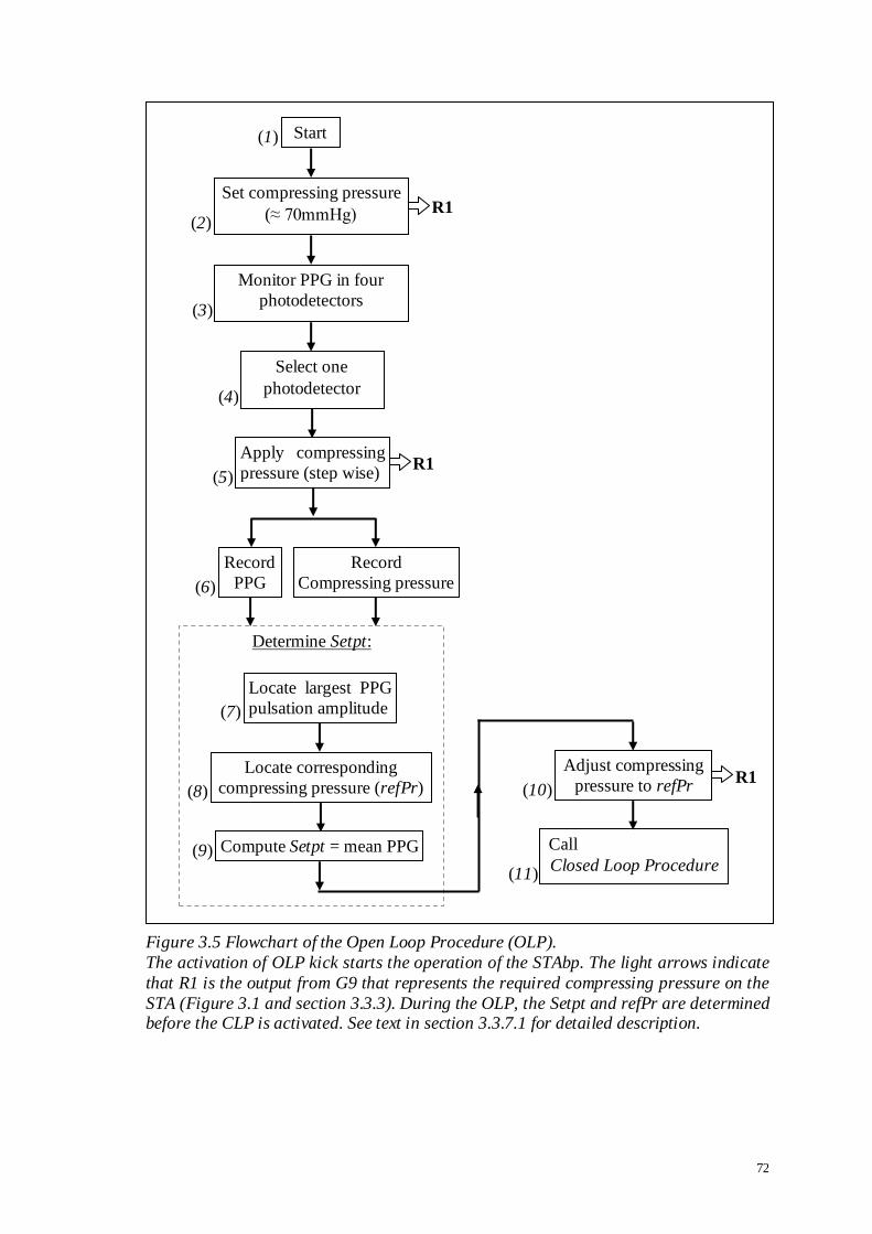
72
Figure 3.5 Flowchart of the Open Loop Procedure (OLP).
The activation of OLP kick starts the operation of the STAbp. The light arrows indicate
that R1 is the output from G9 that represents the required compressing pressure on the
STA (Figure 3.1 and section 3.3.3). During the OLP, the Setpt and refPr are determined before the CLP is activated. See text in section 3.3.7.1 for detailed description.
R1
(1)
(2)
(3)
(4)
(5)
(6)
Record
PPG
Apply compressing
pressure (step wise)
Record
Compressing pressure
Start
Set compressing pressure
(≈ 70mmHg)
Monitor PPG in four
photodetectors
Select one
photodetector
(7)
(8) (10)
(11)
Determine Setpt:
Locate corresponding
compressing pressure (refPr)
Locate largest PPG
pulsation amplitude
Compute Setpt = mean PPG
Adjust compressing
pressure to refPr
Call
Closed Loop Procedure
R1
R1
(9)

73
3.3.7.2 Closed Loop Procedure
CLP is activated immediately after the OLP. The continuous ABP monitoring is
temporarily interrupted from time to time by the CLP subfunction, Setpt Self-Update, to
obtain an updated Setpt. The time interval between consecutive Setpt re-evaluation is
dependent on the absolute percentage change between consecutive Setpt. The default
timer duration is 10s.
Figure 3.6 shows the flowchart of the CLP. The Setpt determined during the OLP is
output as R2 from G9 to G10 (1). The ABP is monitored continuously (3) until the timer
is up (4). When the timer is up, the absolute percentage difference between consecutive
Setpt is compared (5). If the absolute percentage difference is within 10%, the timer
duration is increased at 5s increment steps (6). Otherwise, it is reset to its default 10s
(7). This new timer duration is only used after the operation of the subfunction is
complete (8) and it returns to the beginning of the CLP (2). The CLP is repeated in a
loop until it is externally terminated by the operator. When the CLP is terminated, it
indicates the end of the continuous ABP monitoring with the STAbp.
Figure 3.7 shows the flow chart of the Setpt Self-Update subfunction. The subfunction
temporarily interrupts the operation of the CLP to determine a new Setpt. The range of
compressing pressures used to re-evaluate the Setpt is narrower than the range in OLP.
The compressing pressure in the sealed air chamber (G7) is first reduced (1) by 10
mmHg below the latest recorded mean ABP or the refPr, whichever is lower. It is then
increased in steps of 2 mmHg/s until it reaches 10 mmHg above the latest recorded
mean ABP or the refPr, whichever is higher (2). During this process, the PPG and
transducer pressure are recorded simultaneously (3). These waveforms are analysed

74
immediately after the required range of compressing pressure is applied to determine a
new Setpt. The PPG pulse with the largest pulsation amplitude is first located (4). The
corresponding compressing pressure is retrieved as refPr (5). The mean of the PPG
pulse with the largest pulsation amplitude is computed as the Setpt (6). This is followed
by adjusting the compressing pressure to refPr (7). The CLP is then resumed (8) to
continue with the ABP monitoring.

75
previous Setpt
|current Setpt – previous Setpt| x 100% < 10%?
Is
Call
Setpt Self-Update
Reset timer
(4)
(5)
Increase timer duration
Yes
No
Timer is up?
Yes No
(8)
(6) (7)
Update timer duration
initial Setpt (2)
(3)
Retrieve Setpt (1)
Monitor ABP
R2
Figure 3.6 Flowchart of the Closed Loop Procedure (CLP).
The ABP is monitored continuously during CLP with the specified timer duration. The absolute percentage change of consecutive Setpt is calculated to check if it is within
10%. If it is, the timer duration is increased by 5s. This new timer duration is only used
when the sequence returns to the beginning of the CLP (indicated as „2‟). Otherwise,
the timer is reset to its default duration, i.e. 10s. The Setpt Self-Update subfunction is then activated to update the Setpt value. The CLP repeats in a loop until it is externally
terminated by the operator to indicate the end of the continuous ABP monitoring. The
light arrow indicates output of R2 from G9. R2 is the Setpt. See text in section 3.3.7.2
for detailed description.
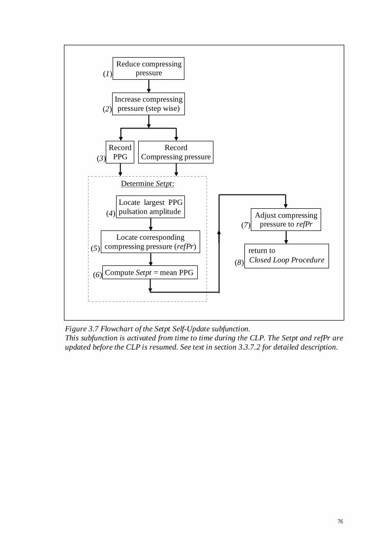
76
Figure 3.7 Flowchart of the Setpt Self-Update subfunction.
This subfunction is activated from time to time during the CLP. The Setpt and refPr are
updated before the CLP is resumed. See text in section 3.3.7.2 for detailed description.
Reduce compressing pressure
Increase compressing
pressure (step wise)
Record
PPG
Record
Compressing pressure
Determine Setpt:
Locate corresponding
compressing pressure (refPr)
Locate largest PPG
pulsation amplitude
Compute Setpt = mean PPG
Adjust compressing pressure to refPr
return to
Closed Loop Procedure
(1)
(2)
(3)
(4)
(5)
(7)
(8)
(6)

77
3.4 Initial Assessments
Section 3.3 described the instrumentation of the STAbp prototype. The design criteria
highlighted in section 3.2 are incorporated into the prototype. The following subsections
describe two assessments on the STAbp, i.e. the frequency response test and the
prototype device safety evaluation.
3.4.1 Frequency Response Test
Referring to the description of G3 in section 3.3.3 (see also Figures 3.1 and 3.4), G3
consists of five sub-blocks (G4 to G8), which form a local feedback control loop to
linearise the compressing pressure in the probe as required by input R1 (or C3). As
explained in section 3.3.3, pressure hysteresis will occur if the piezo valve (G6) is used
alone.
An experiment was set up to assess the frequency response of G3. The setup is
illustrated in Figure 3.8. The front end surface of the probe is placed on the surface of a
workbench with a gap of approximately 1.0 mm. The gap distance was arbitrarily
chosen but it is aimed to simulate the distance between the surfaces of the probe and the
skin when an external compressing pressure is applied on the tissue. The probe is fixed
with a clamp and the clamp is fastened against a supporting stand. A mean compressing
pressure of 75 mmHg with sine wave peak-to-peak amplitude of 60 mmHg was fed to
the input of G3. The sine wave frequency began at 1 Hz and was gradually increased to
100 Hz. During this process, the gain and phase responses were recorded. The
experiment was repeated with mean compressing pressures of 100 and 125 mmHg. The
experimental results are presented in section 3.5.2.

78
Figure 3.8 Experimental setup to evaluate frequency response of G3.
The setup adopted is to evaluate the frequency response of the regulated compressing
pressure (G3) described in section 3.3.3. The front end surface of the probe is placed on
the surface of a workbench. The probe is fixed with a clamp and the clamp is fastened against a supporting stand. See text in section 3.4.1 for detailed description.

79
3.4.2 Device Safety Evaluation
Safety considerations described in section 3.2 raised four device safety issues. The
following describes steps taken to meet these considerations:
a) Upper limit of compressing pressure: the compressing pressure of the sealed air
chamber (G7) is supplied up to 260 mmHg. G7 was tested to withstand air pressure
of at least 350 mmHg. A pressure switch is connected to the mains supply for the
micro air compressor (Figure A.2 in the Appendix). The mains supply to the air
compressor is cut off if the pressure output from the regulated compressed air
supply (G4) exceeds 260 mmHg.
b) Leakage current: the electrical connection at the probe is powered with an isolated
voltage supply to prevent current leakage to flow through the subject. The isolation
can withstand up to 1500Vrms (Burr-Brown, 1997).
c) Tissue heating: IRED with low current consumption is used to minimise local
heating on the temporal tissue (section 3.3.1). Initial trial had no reported sensation
of heating or redness on the skin. This will be reassessed in chapter 4 when the
STAbp was tested in a group of healthy subjects (section 4.6.5).
d) Risk of tissue ischaemia: multiple large and soft paddings fastened around the head
with the head frame provide evenly distributed pressure on the scalp tissue (section
3.3.2). Initial trial had not shown evidence of pain, dizziness or other discomfort.
This will be reassessed in chapter 4 when the STAbp was tested in the group of
subjects to obtain their feedback (section 4.6.5).

80
3.5 Results
Following the descriptions of the operations with the Open- and Closed- Loop
Procedures in section 3.3.7, the results of the preliminary testing are presented in the
following. The results of the frequency response test described in section 3.4.1 are
presented in subsection 3.5.2.
3.5.1 Open Loop Operation
Figure 3.9 illustrates an example of recorded transducer pressure and PPG waveforms
during the OLP to determine the Setpt. The compressing pressures encompass the
physiological range of systolic and diastolic pressures. The PPG pulse with the largest
pulsation amplitude is located. The Setpt is computed as the mean of this PPG pulse.
The corresponding compressing pressure value is retrieved as refPr. Once the Setpt and
refPr are obtained, the OLP is complete. It is immediately followed by the CLP.
3.5.2 Frequency Response
Figure 3.10 shows the frequency response of the regulated compressing pressure (G3).
The gain did not drop below the conventional -3 dB point within the 0 to 100 Hz
frequency range. It only began to drop below zero dB at frequencies above 40 Hz.
Similarly, the phase shift started to lag from -10º only when the frequency had increased
to at least 25 Hz. The graphs show three curves at mean compressing pressures of 75,
100 and 125 mmHg respectively. The frequency response is scarcely affected by the
level of the mean compressing pressures.

81
Figure 3.9 Recorded PPG waveform during Open Loop Procedure (OLP). (a) Transducer pressure recording; (b) simultaneous recording of PPG waveform. The
PPG pulse with the largest pulsation amplitude is first located (indicated as „1‟). The
Setpt is computed as the mean of this PPG pulse. The corresponding compressing
pressure value is retrieved as refPr (indicated as „2‟).
Setpt
refPr
(a)
(b)
(2)
(1)

82
Figure 3.10 Frequency response curves of the regulated compressing pressure (G3). The gain (a) and phase (b) responses are shown. Three mean compressing pressures
were applied: 75 (diamond), 100 (triangle) and 125 (cross) mmHg with peak-to-peak
sinusoidal amplitude of 60 mmHg. The gain response shows that it only began to drop
below zero dB at frequencies above 40 Hz. Correspondingly, the phase shift started to lag from -10º only at frequencies above 25 Hz.
(a)
(b)

83
3.5.3 Closed Loop Operation
Figure 3.11 shows a representative paired recording of the STAbp on the right STA and
the Finapres on the right middle finger for 16 cardiac cycles. Finapres ABP was used
for comparison. They were measured from a healthy adult while sitting in an upright
position on a chair with back support. Hydrostatic pressure difference was taken into
account when the waveforms were recorded.
Figure 3.12 shows a representative ABP trace of the STAbp and Finapres in response to
the Valsalva manoeuvre (Looga, 2005; Nishimura and Tajik, 1986; Taylor, 1996).
Simultaneous variation of the ABP can be observed. This shows that the STAbp is able
to track the ABP changes during the manoeuvre.
These measurement results are only illustrative. A more formal assessment will be
presented in chapter 4.
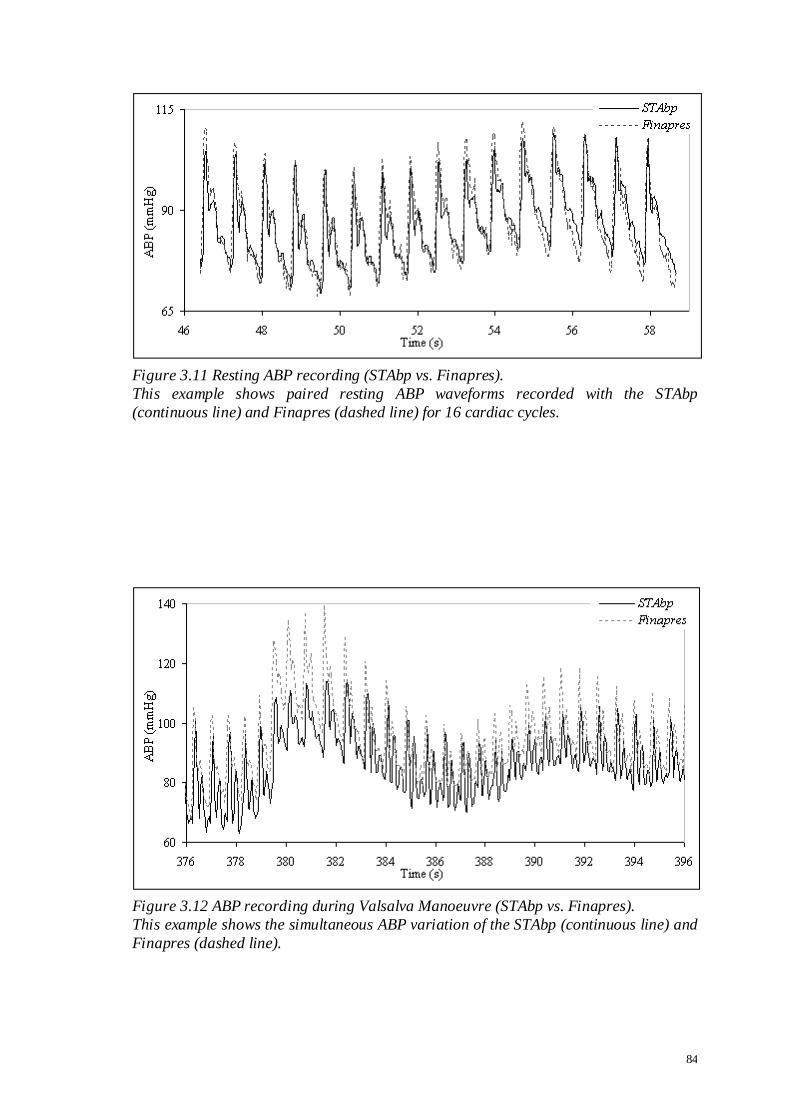
84
Figure 3.11 Resting ABP recording (STAbp vs. Finapres).
This example shows paired resting ABP waveforms recorded with the STAbp
(continuous line) and Finapres (dashed line) for 16 cardiac cycles.
Figure 3.12 ABP recording during Valsalva Manoeuvre (STAbp vs. Finapres).
This example shows the simultaneous ABP variation of the STAbp (continuous line) and
Finapres (dashed line).

85
3.6 Discussion
The instrumentation of the STAbp was described in section 3.3. Preliminary
measurement results were shown in section 3.5. In the following paragraphs, four areas
of the device development are discussed. These refer to the quality of the PPG
waveform, the arrangement of optoelectronic components in the probe, area of
compression on tissue, and the frequency response test of G3.
PPG waveform
The PPG signal is generated when the scattered or reflected light from the tissue
illuminated by the IRED reaches the photodetector. Factors that can affect the quality of
the PPG waveform include:
the absorption and scattering properties of the arterial blood, surrounding tissue and
the temporal bone beneath the tissue. It is assumed that these properties in the
surrounding tissue and bone remain constant. Hence, the fluctuation observed in the
PPG is only caused by the blood volume pulsation in the STA;
the depth of artery from skin surface along the temporal region. It is assumed that
the depth remains constant and the arterial dimension is uniform. Otherwise, it could
affect the optical pathway of the light illumination;
the distance between the artery and optoelectronic components. It is assumed that
the distance remains the same throughout the continuous ABP monitoring;
due to tissue elasticity, the artery may be pushed away from the optoelectronic
components as the compressing pressure increases. This can change the initial
distance and the optical pathway. It is assumed that this distance stays the same;

86
interferences such as motion artefacts, electronic noise, change of temperature in the
surroundings and change of ambient lighting. Strong ambient lighting with similar
emitting wavelength as the IRED could potentially drive the current in the
photodetector to saturation;
pulse pressure. Decreased pulse pressure or weak pulse tends to give smaller PPG
pulse amplitude, thus worsening the signal-to-noise ratio;
physical characteristics of optoelectronic components, e.g. lens of the IRED which
directs the illumination, intensity of emitted light and photosensitive active area in
the photodetector;
potential venous pulsation from blood vessels nearby, e.g. superficial temporal vein.
All the above factors could be seen as potential limitations and their validity should be
the object of further scrutiny.
Optoelectronics in the probe
As described in section 3.3.1, four photodetectors are fitted inside the probe. It was then
described in section 3.3.7.1 that only one photodetector is used during continuous ABP
monitoring. This design offers the advantage to search the location of the STA with
more confidence based on the quality of the PPG waveforms before continuous ABP
monitoring begins.
However, it is not possible to identify the exact location and orientation of the STA. The
possible placements of the IRED and the four photodetectors (PD) inside the probe
relative to the STA are shown in Figure 3.13. In placement 1, the IRED, PD1 and PD3
are placed directly over the STA. In placement 2, the IRED and PD1 to PD3 are placed
at approximately the same distance from the artery, but the optical pathway for PD2

87
may be different as compared for PD1 and PD3. In placement 3, PD2 is directly over
the STA; however, the IRED is relatively further away from the artery. Lastly, in
placement 4, the IRED is placed directly over the STA while the distances of all the
four PD from the artery are relatively further away.
These possible placements generally illustrate that the optical pathway is different when
the position of the optoelectronic components relative to the STA is changed. These
could lead to a different PPG amplitude and waveshape recorded, and potentially a
poorer quality of the ABP waveform is produced. Furthermore, section 3.3.1 described
that a dome shape is produced when the sealed air chamber (G7) is fully inflated. The
STA may not always be aligned on the tip of the dome. This may then pose as a
limitation for the STAbp as the STA may not be evenly compressed. Placement 1 is
probably the best in terms of optical pathway and uniformity of compression.
To understand better the optical pathway and the compression on the tissue with the
underlying STA, further work will be required. For instance, mathematical modelling
may be beneficial or to construct a specific experimental test rig to learn more about the
properties of the optical pathway and effect of uneven compression on the PPG and
ABP measurements. These further works are not presented in the subsequent chapters as
they are beyond the scope of the thesis.
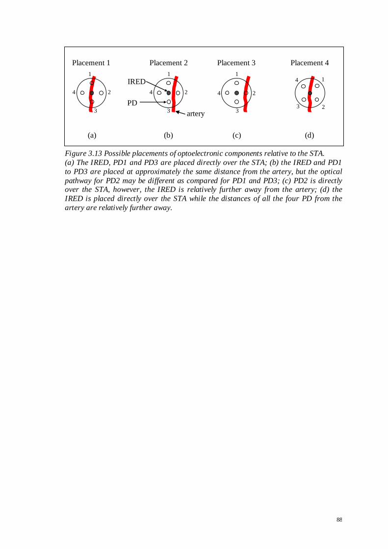
88
Figure 3.13 Possible placements of optoelectronic components relative to the STA.
(a) The IRED, PD1 and PD3 are placed directly over the STA; (b) the IRED and PD1
to PD3 are placed at approximately the same distance from the artery, but the optical
pathway for PD2 may be different as compared for PD1 and PD3; (c) PD2 is directly over the STA, however, the IRED is relatively further away from the artery; (d) the
IRED is placed directly over the STA while the distances of all the four PD from the
artery are relatively further away.
Placement 1
1
2
3
4
(a) (b) (c) (d)
Placement 3 Placement 2
IRED
PD
1
2
3
4
artery
1
2
3
4
Placement 4
1
2 3
4
89
Area of compression on tissue
In addition to the dome shape of the inflated sealed air chamber, the area of
compression on tissue may affect the effectiveness of pressure transmission through the
tissue. In the Finapres and many arm-cuff oscillometric measurement devices, different
cuff sizes are provided to cater for different dimensions of the measurement site, for
instance, the circumference of the finger or the upper arm (Boehmer, 1987; Hirai et al.,
1976; Imholz et al., 1998; Jones et al., 1993). It is well known that inappropriate cuff
size leads to inaccurate ABP measurements (Geddes and Whistler, 1978; Manning et
al., 1983; Ng and Small, 1993). The same physical principles may apply to the STA in
the temporal region. The current area of compression of the probe in the STAbp has a
diameter of 18 mm. Further work may be necessary to investigate the effect of different
areas of compression on the accuracy of ABP measurement.
Frequency response of G3
Referring to Figure 3.1 and section 3.4.1, the limitation of the frequency response test is
that only the frequency response of the regulated compressing pressure (G3) was tested
instead of the complete integrated device. The frequency response test of the integrated
device requires R2 (= Setpt) as the control input, C1 (= real time PPG) as the control
loop feedback signal, and G10 as the feedback controller. Such arrangement requires
living tissue as part of the closed loop. The frequency response may consequently be
considered unreliable due to changes in physiological conditions and mechanical
properties of the tissue within- and between individuals. This limitation will be
addressed again when the frequency response and magnitude squared coherence
analyses are described in chapter 4.

90
3.7 Conclusion
The design and instrumentation of the STAbp prototype demonstrates the integration of
different hardware and software components to monitor the ABP continuously.
Relevant design criteria were considered and they were incorporated into the device.
Initial assessments on the STAbp shows that appropriate steps have been taken to ensure
safety of use in human subjects. Preliminary results show that the ABP waveforms
measured with the STAbp are comparable against the Finapres. A more formal
assessment of the STAbp on a group of subjects will be presented in the next chapter.
91
CHAPTER 4 PROTOTYPE DEVICE EVALUATION
4.1 Introduction
Chapter 3 described the system architecture of the STAbp prototype. Preliminary
measurement results showed that it was satisfactory to carry out a more formal
assessment with more human subjects.
A separate measurement device is required to evaluate the STAbp. The best option
would be the gold standard, which is intravascular measurement. However, due to the
high risk of infection, other clinical complications and costs implications (Bedford and
Wollman, 1973; Carroll, 1988; Murray, 1981; Puri et al., 1980), it was deemed safer to
first evaluate the STAbp against another noninvasive device. This approach also offers
the opportunity to further understand the practical use of the new measurement device,
to identify and make necessary improvements or modifications to the prototype before it
is evaluated against an intravascular counterpart.
In this chapter, Finapres was chosen as the reference noninvasive measurement device
for STAbp. An overview about the accuracy and reliability of the Finapres was given in
several publications for a wide range of pathological and physiological conditions and
in subjects of different age groups (Imholz et al., 1998; Wesseling, 1995; Wesseling et
al., 1995). It is to note that the accuracy of the Finapres itself was evaluated against
another measurement site, whether through invasive or noninvasive methods. Not
surprisingly, discrepancies in ABP will occur due to different measurement locations.

92
Sections 1.1 and 1.2.3 mentioned that arterial pressure waveforms in different arteries
are susceptible to the effect of pulse wave propagation and reflection. Also, there is
usually a small drop in mean pressure in peripheral arteries. The ideal design would be
to evaluate the Finapres against an intravascular measurement on a finger artery.
However, such literature could not be found.
The Finapres is the next best option available after the intravascular measurement
technique to evaluate the STAbp. Prior to this evaluation, two Finapreses of the same
specifications and model number (Ohmeda 2300) were first compared to assess their
inherent differences. The results were then used to define appropriate boundaries when
interpreting the comparative study of the STAbp and Finapres.
The objectives of this chapter are:
i. To describe data analysis techniques common to both comparative studies (section
4.2). Analysis techniques specific to a comparative study will be described in
respective sections 4.3 and 4.4;
ii. To describe the comparative study of two Finapreses, followed by analysis results
(section 4.3). The Finapreses are referred to as Finap1 and Finap2, with Finap1 as
the reference;
iii. To describe the comparative study of the STAbp and Finapres, followed by analysis
results (section 4.4). The same Finap1 was used as reference;
iv. To further compare the analysis results between both comparative studies (section
4.5), followed by discussion (section 4.6) and conclusion (section 4.7).

93
4.2 Data Analysis Techniques
The data analyses carried out for both comparative studies are very similar. This is to
enable direct comparisons of results between both studies and to interpret the
differences accordingly. This section describes analysis techniques common to both
studies, whereas analysis techniques specific to a single comparative study will be
described in that section.
In each comparative study, analyses were based on two types of physiological
conditions, i.e. resting ABP and the ABP dynamic change due to activity. The ABP at
both measurement sites were recorded simultaneously by two monitoring devices. The
two devices will be initially denoted as reference device A and test device B in this
section. They will be specified clearly later in each comparative study. The ABP
waveforms were each digitally sampled at 200 Hz, operated with a desktop computer
incorporating the Agilent VEEPro® 6.2 software.
Four parameters of the resting ABP will be evaluated. They are the agreement between
simultaneously recorded ABP waveforms, frequency bandwidth of ABP pulses,
frequency response and magnitude squared coherence analyses, and the assessment of
ABP drift. Furthermore, the agreement between ABP waveforms during a dynamic
change due to activity was also assessed. These five parameters will be described in the
following subsections.
Comparison between the two devices were performed within the analysis of agreement
framework proposed by Bland and Altman (1986). The statistical parameters to report
included the mean of differences (bias), standard deviation of differences (SD), limits of
94
agreement and the root mean squared error (RMSE). A value of p <0.05 was taken as
the level of statistical significance. This criterion applies to all statistical analyses in this
chapter.
4.2.1 Resting ABP: Agreement
Simultaneously recorded (or paired) resting ABP waveforms were recorded by devices
A and B for several minutes in each subject. 16 cardiac pulses at the beginning of the
recording were retrieved for analysis. This range was selected to avoid non-stationarity
of the ABP waveforms.
Starting with device A recording, 16 systolic, mean and diastolic pressure values (SBP,
MAP and DBP respectively) were calculated from the selected range of ABP waveform.
The detections of these pressure values were produced automatically with a software
programme developed in-house. An average was then computed for the SBP, MAP and
DBP values respectively. The same process was repeated for device B recording. The
differences between each pair of SBP, MAP and DBP averages were computed for each
subject. Bias (SD) was then computed from all subjects’ differences for the SBP, MAP
and DBP respectively. The corresponding mean (SD) of all subjects’ RMSE were also
computed.
4.2.2 Resting ABP: Bandwidth
The frequency content of an ABP pulse waveform recorded at rest can be influenced by
factors such as the physiological conditions of the measurement site, heart rate, cardiac

95
function and pulse wave propagation and reflection. It was suggested that a minimum of
six harmonics is sufficient to reconstruct the original pressure wave with relatively close
agreement (O'Rourke and Nichols, 2005).
In this section, the frequency content of a resting ABP pulse is quantified as the
bandwidth containing either the 95% or the 99% of its total spectral power. To compute
these bandwidth limits, the power spectrum is required. It is assumed that the pulse
duration and waveshape of consecutive resting ABP pulses are approximately the same.
The discrete Fourier transform (DFT) of individual ABP pulses was first computed. The
DFT is given by
1
0
/2)(N
n
Nnkjnk exfX
(4.1)
where N is the sample size of an ABP pulse. xn refers to the sampled ABP values for n =
0, 1, 2, …, N-1. k = 0, 1, 2, …, 2
N is the array for the frequency values (fk) from zero to
half the sampling frequency (fs); this gives (2
N+1) number of fk values which
represents the positive half of the transformed values. The frequency interval is
dependent on N and fs, i.e. in the increment of N
f s . Therefore, each frequency value
plotted along the abscissa is N
kff s
k (Bendat and Piersol, 1986; Brigham, 1988). For
simplicity, the subscript k in fk will not be shown in the following text, i.e. X(fk) = X(f).
X(f) is usually a complex number. For an ABP measured with the reference device A,
let GAA(f) represents the discrete power spectrum given by

96
GAA(f) =A*(f)∙A(f) ≡ 2Im
2Re )()( fAfA ≡
2)( fA (4.2)
where A(f) replaces X(f) in Equation 4.1. A*(f) is the complex conjugate of A(f). A
normalised cumulative power spectrum for the ABP pulse was then computed and the
95% and 99% bandwidth limits were identified. Linear interpolation was used for a
bandwidth limit between frequency points.
The same computation process was repeated for test device B. Similar to Equation 4.2,
the power spectrum for test device B is given by
GBB(f) =B*(f)∙B(f) ≡ 2Im
2Re )()( fBfB ≡
2)( fB (4.3)
where B*(f) is the complex conjugate of B(f).
The same 16 paired ABP pulses selected in section 4.2.1 were used to compute the 95%
and 99% bandwidth limits. The following explains the step-by-step computation
process:
1. compute the 95% bandwidth limit from each of the 16 ABP pulses recorded with
reference device A (denoted as 95,AK );
2. compute an intra-subject average from step 1 (16
16
1,95,
95,
m
mA
A
K
K );
3. compute the 95% bandwidth limit from each of the 16 ABP pulses recorded with
test device B (denoted as 95,BK );
4. compute an intra-subject average from step 3 (16
16
1,95,
95,
m
mB
B
K
K );
5. compute intra-subject difference for 95% bandwidth limit ( 95,95,95 AB KKK );
6. repeat steps 1 to 5 to obtain 95,AK , 95,BK and 95K for all subjects;
7. compute respective mean (SD) of 95,AK and 95,BK ;

97
8. repeat steps 1 to 7 for 99% bandwidths to obtain 99,AK , 99,BK and 99K for all
subjects;
9. compute respective mean (SD) of 99,AK and 99,BK .
4.2.3 Resting ABP: Frequency Response and Magnitude Squared Coherence
The frequency response test described in section 3.4.1 only applies to the block G3 in
the STAbp system architecture (Figure 3.1 and section 3.3.3). G3 provides regulated
compressing pressure in the probe to compress the STA. The probe was described in
section 3.3.1.
The frequency response test was not carried out on the whole STAbp device as it needs
to incorporate the living tissue component, which may vary within- and between-
individuals. For this reason, the frequency response of the STAbp device was assessed
by a frequency response analysis using the Finapres signal as input.
The frequency response analysis is useful to estimate the dynamic relationship between
paired recordings of ABP waveforms in the frequency domain. The computation of the
frequency response will give the gain and phase spectra. The magnitude squared
coherence is complementary to the frequency response analysis to assess for consistent
frequency coupling between the paired ABP waveforms. The spectral comparison
between two Finapreses will give the frequency response that can be used as reference
when interpreting the frequency response in the spectral comparison between the STAbp
and Finapres.

98
To compute the frequency response (H(f)) and the magnitude squared coherence (γ2(f)),
the auto- and cross- spectra were first computed. The ABP waveforms from the
reference device A and test device B were the input and output functions respectively.
The auto (power) spectra GAA(f) and GBB(f) have been given in Equations 4.2 and 4.3.
The cross spectrum (GAB(f)) is given as
GAB(f) =A*(f)∙B(f) (4.4)
In theory, H(f) and )(2 f are defined as )(
)()(
fG
fGfH
AA
AB and
)()(
)()(
2
2
fGfG
fGf
BBAA
AB
respectively. However, due to the presence of noise
component in real time signals, the auto- and cross- spectra were first computed from
individual fast Fourier transform (FFT) of 16 windowed ABP waveform segments, and
then averaged (Bendat and Piersol, 1993; Brigham, 1988). The number of windows was
not increased to avoid potential non-stationarity of the waveform. Each window of ABP
waveform consists of 512 sample points, corresponding to 2.56s. This approach allows
the use of stable segments of the ABP waveform which always include at least one
complete cardiac cycle and also to smoothen the spectral estimates.
Before the FFT was applied, the mean of the windowed waveform was first removed.
Each windowed waveform was then multiplied with a 20% cosine-tapered Hanning
window (Bloomfield, 2000; Harris, 1978). This overcomes the discontinuity of
windowed waveform, hence spectral leakage is minimised. After multiplication by the
Hanning window, the residual mean of the tapered waveform was further removed to
obtain zero offset. This process was repeated for 16 windows with 50% Welch

99
overlapping from the continuous ABP waveform (Oppenheim and Schafer, 1975;
Proakis and Manolakis, 1996). There are other advantages of using a windowed ABP
waveform. One is to overcome the variation of pulse duration, and the other is to retain
the phase difference between the paired waveforms.
To apply H(f) and )(2 f in practice, if m is the number of windowed ABP waveform
segments from each ABP recording, the estimates of H(f) and f2 now become
m
iiAA
m
iiAB
fG
fG
fH
1
1
)(
)(
)(ˆ (4.5)
m
iiBB
m
iiAA
m
iiAB
fGfG
fG
f
11
2
12
)()(
)(
)(̂ (4.6)
As )(ˆ fH is usually complex, the average gain (| )(ˆ fH |) and phase ( )(ˆ f ) spectra can
be obtained from the real part Re)(ˆ fH and imaginary part Im)(ˆ fH , as
21
2
Im
2
Re )(ˆ)(ˆ)(ˆ
fHfHfH and
Re
Im1
)(ˆ
)(ˆtan)(ˆ
fH
fHf respectively. The
upper frequency bandwidth was identified at the gain of 0.707, which is equivalent to
the conventional -3 dB cut-off frequency. The minimum level of acceptance for the
magnitude squared coherence was chosen at 0.5 as a conservative criterion which is
widely used in the literature (de Boer et al., 1985).

100
4.2.4 Resting ABP: Assessment of Drift
The assessment of drift in ABP measurement describes the agreement of paired ABP
waveforms after the resting ABP is monitored for several minutes. To quantify drift, the
difference between percentage changes in the paired ABP waveforms was calculated.
The percentage change in ABP is denoted as Ψ (unit is %). The generic equation is
derived as
Ψi DBPMAPSBP ,, %100)(
)()(
begini
beginiendi
P
PP DBPMAPSBP ,, (4.7)
i refers to reference device A or test device B. iP is an average calculated from 16
cardiac pulses. Ψi was computed for SBP, MAP and DBP.
The same 16 cardiac pulses selected in section 4.2.1 were used for )(beginiP . Another 16
cardiac pulses towards the end of the same recorded waveform were selected for )(endiP .
The difference (= ΨB - ΨA) was calculated for each subject. The mean (SD) of ΨA,
ΨB and from all subjects were then computed for SBP, MAP and DBP.
4.2.5 ABP Dynamic Change during Activity
The above sections 4.2.1 to 4.2.4 described analysis techniques on resting ABP
waveforms. This section describes the assessment on the agreement of paired ABP
waveforms with dynamic change due to specific manoeuvres. The comparative studies
described in sections 4.3 and 4.4 carried out two different activities to assess this type of
agreement. In section 4.3, a Valsalva manoeuvre was conducted, whereas in section 4.4,
an isometric handgrip (IHG) exercise was conducted. The choice of activity was

101
different because a Valsalva manoeuvre may interfere with the ABP measurement in the
STA, for example, the motion artifacts due to upper body or jaw movement during the
manoeuvre could have a larger interference on the STAbp device. Thus, it was replaced
by the IHG exercise. For similar reason, IHG exercise was not carried out for the finger
ABP measurements as both hands were needed for finger cuff fitting.
To quantify the agreement of ABP dynamic change, the difference between percentage
changes in the paired ABP waveforms was calculated. The percentage change in ABP is
denoted as Φ (unit is %). The generic equation is derived as
Φ i,j DBPMAPSBP ,, %100)(,
)(,)(,
beginji
beginjiendji
P
PP DBPMAPSBP ,, (4.8)
i refers to reference device A or test device B; j refers to Valsalva manoeuvre (VM) or
the IHG exercise (IHG). jiP, is an average calculated from 10 cardiac pulses. Φi,j was
computed for SBP, MAP and DBP. The difference ( j = ΦB,j - ΦA,j) was calculated
for each subject. The mean (SD) of ΦA,j, ΦB,j and j from all subjects were then
computed for SBP, MAP and DBP.
Valsalva manoeuvre (for section 4.3 only)
)(, beginVMiP refers to the average from 10 cardiac pulses prior to the strain of the
manoeuvre. )(, endVMiP refers to the average from 10 cardiac pulses at the peak of phase
IV after the strain was released (Looga, 2005; Nishimura and Tajik, 1986; Taylor,
1996).

102
IHG exercise (for section 4.4 only)
)(, beginIHGiP refers to the average from 10 cardiac pulses prior to the beginning of the
handgrip. )(, endIHGiP refers to the average from 10 cardiac pulses just before the handgrip
was released.
103
4.3 Comparative Study of two Finapreses
Paired ABP measurements with two Finapreses of the same model will be described in
this section. This is to characterise their inherent differences before the STAbp is
evaluated. The two Finapreses are referred to as Finap1 (device A) and Finap2 (device
B) with Finap1 as reference.
4.3.1 Method
11 subjects were recruited for this study (6 males, 5 females, age (mean ± SD) 36 ± 12
years). The participants were all staff from the Medical Physics department. Consent
was given by each participant prior to the arrangement for the ABP measurements. The
study was approved by the Leicestershire ethics committee (reference number: 4680).
Each subject was requested to avoid stressful activities prior to the ABP measurement.
The subjects had no history of conditions affecting their hands or its circulation. Each
subject sat on a chair with back support. Both hands were resting comfortably on a
bench at the same height as the heart level. The room temperature was maintained at
approximately 22 ºC. Two fingers from a combination of middle and annulus fingers of
both hands were selected. With two Finapreses and two fingers selected for ABP
measurements, there are twelve possible combinations (Table 4.1). Only four out of the
twelve possible combinations were tested in this study, indicated as Tests #1 to Test #4
in bold in the table. The sequence of the four tests was randomised with a lapse of at
least 30 minutes apart between tests to allow the fingers to rest.
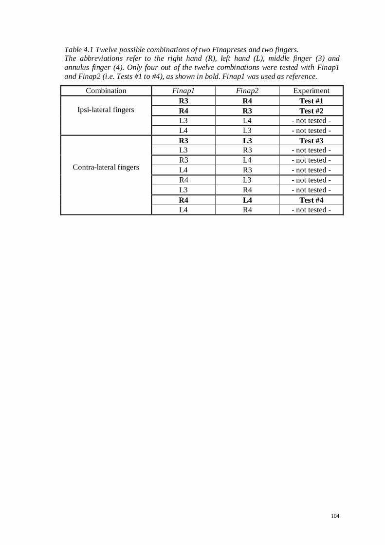
104
Table 4.1 Twelve possible combinations of two Finapreses and two fingers. The abbreviations refer to the right hand (R), left hand (L), middle finger (3) and
annulus finger (4). Only four out of the twelve combinations were tested with Finap1
and Finap2 (i.e. Tests #1 to #4), as shown in bold. Finap1 was used as reference.
Combination Finap1 Finap2 Experiment
Ipsi-lateral fingers R3 R4 Test #1
R4 R3 Test #2
L3 L4 - not tested -
L4 L3 - not tested -
Contra-lateral fingers
R3 L3 Test #3
L3 R3 - not tested -
R3 L4 - not tested -
L4 R3 - not tested -
R4 L3 - not tested -
L3 R4 - not tested -
R4 L4 Test #4
L4 R4 - not tested -

105
Each selected finger was fitted with a suitable Finapres cuff according to the guidelines
provided by the manufacturer. The ABP in both fingers were monitored simultaneously
with the Finapreses. The subject was asked to relax and breathe normally during ABP
measurements. The ABP was monitored for several minutes until the ABP was stable.
The Finapres has the capability to self-calibrate during continuous ABP monitoring,
known as Physiocal (Wesseling et al., 1995). When stable ABP waveforms were
obtained in both recorders, this feature in both devices was temporarily switched off
before the recording began.
Each paired ABP recording lasted for 4 min. At the second minute, a Valsalva
manoeuvre was performed and lasted for approximately 20s (Dawson et al., 1997;
Dawson et al., 1999a; Weston et al., 1996a). 16 cardiac pulses at the beginning and 16
cardiac pulses towards the end of the 4 min recording were retrieved. The analysis
techniques for these ranges of waveforms were described in sections 4.2.1 to 4.2.4. The
recorded waveforms during the Valsalva manoeuvre were analysed with the approach
described in section 4.2.5.
The following paragraph describes statistical computations specific to this comparative
study in addition to the techniques described in section 4.2. For each parameter
considered, the null hypothesis states that there is no statistical significance between
mean values.
The two Finapreses and the combination of two fingers’ ABP measurements (Tests #1
to #4) gave a ‘2 way 4 levels’ design. A two-way within subjects (repeated measures)
analysis of variance (ANOVA) was carried out to test the main hypothesis (Roberts and

106
Russo, 1999). The ANOVA factors were denoted as ‘Finap’ (2 levels) and ‘Test’ (4
levels). If the null hypothesis was rejected, post hoc Scheffe testing (Maxwell and
Delaney, 2004; Roberts and Russo, 1999) was carried out and the four tests were
assessed separately. Conversely, if the null hypothesis was accepted, the measurement
results were pooled.
4.3.2 Results
Paired ABP recordings from 11 subjects (Tests #1 to #4) were all of good quality. The
resting ABP were stable during the 4 min recording with a clear dynamic change in the
second minute during the Valsalva manoeuvre. No waveforms were excluded from the
analysis.
The presentation of results follows the sequence described in section 4.2 and adopts the
same headings. Figure 4.1 shows an example of the paired resting ABP recordings with
16 cardiac pulses at the beginning and 16 cardiac pulses towards the end of the 4 min
recording respectively. The former waveform segment was analysed according to the
first three data analysis techniques described in sections 4.2.1 to 4.2.3. Both waveform
segments were then analysed for the assessment of drift according to the technique
described in section 4.2.4. Lastly, the analysis technique described in section 4.2.5 was
used for the assessment of the ABP dynamic change during Valsalva manoeuvre. An
example recording during the Valsalva manoeuvre is shown in Figure 4.2.

107
Figure 4.1 Resting ABP waveforms (Finap2 vs. Finap1).
Example of 16 cardiac pulses at the beginning (a) and 16 cardiac pulses towards the end (b) of a 4 min recording with Finap2 (black continuous line) and Finap1 (grey
dashed line). Finap1 was used as reference.
(a)
(b)

108
Figure 4.2 ABP waveforms during Valsalva manoeuvre (Finap2 vs. Finap1).
Example of (a) Finap1 recording; (b) Finap2 recording; (c) Finap2 (black continuous line) and Finap1 (grey dashed line). Finap1 was used as reference. The arrows show
the beginning and end of the Valsalva manoeuvre. Phase IV (as indicated in the graphs)
is the classical ABP overshoot observed upon release of the expiratory strain.
(a)
(b)
(c)
phase IV
phase IV
phase IV

109
4.3.2.1 Resting ABP: Agreement
The statistical analysis results for the agreement between paired resting ABP waveforms
are presented as follows:
Tables 4.2 to 4.4: ANOVA results with p-values (2 ways 4 levels design) for SBP,
MAP and DBP. Significant values are printed in bold. Consequently, the null
hypothesis was rejected and the tables have included results of post-hoc Scheffe
testing.
The ANOVA results show significant differences in the ‘Finap’ main effect for SBP
(p=0.010), MAP (p=0.008) and DBP (p=0.021). Significant differences were
obtained in the ‘Test’ main effect for SBP (p=0.030) and MAP (p=0.043), but not
for DBP. No significant differences were obtained in the ‘Finap x Test’ interaction
for SBP, MAP and DBP (Tables 4.2(a), 4.3(a) and 4.4(a)).
Post hoc Scheffe tests on the ‘Test’ main effect show no significant differences in
Tests #1 to #4 for SBP, MAP and DBP. However, post hoc Scheffe tests on the
‘Finap x Test’ interaction show six significant values for SBP (Table 4.2(c)), three
for MAP (Table 4.3(c)) and one for DBP (Table 4.4(c)). All the significant p-values
are related to ‘Finap2 Test #1’ (labelled as 5 );
Figure 4.3: plots of means of SBP, MAP and DBP for the ‘Finap’ and ‘Test’ main
effects;
Figure 4.4: plots of means of SBP, MAP and DBP for the ‘Finap x Test’ interaction;
Figures 4.5(a-d): plots of agreement for SBP, MAP and DBP in Tests #1 to #4. The
analysis results for each test were treated separately (i.e. n1 = n2 = n3 = n4 = 11

110
subjects) because the null hypothesis was rejected. The respective regression lines
show no significant correlations;
Table 4.5: bias (SD) for Tests #1 to #4. As shown by the ANOVA, Test #1
presented the largest bias, associated with recordings from Finap2;
Table 4.6: mean (SD) of RMSE for Tests #1 to #4.

111
Table 4.2 ANOVA p-values for SBP (two Finapreses with four tests). (a) ANOVA results for „Finap‟ and „Test‟ main effects, and their interaction; (b) post -
hoc Scheffe test for „Test‟ main effect; (c) post-hoc Scheffe test for „Finap x Test‟
interaction. Significant values are printed in bold.
(a) ANOVA (2 ways 4 levels)
‘Finap’ 0.010
‘Test’ 0.030
‘Finap’ x ‘Test’ 0.162
(b) Test #1 Test #2 Test #3 Test #4
Test #1 -- 0.346 0.062 0.091
Test #2 -- 0.800 0.883
Test #3 -- 0.998
Test #4 --
(c) 1 2 3 4 5 6 7 8
Finap1 Test #1 1 -- 0.984 0.082 0.412 0.272 0.992 0.974 0.859
Finap1 Test #2 2 -- 0.469 0.926 0.035 1.000 1.000 1.000
Finap1 Test #3 3 -- 0.991 0.000 0.408 0.524 0.776
Finap1 Test #4 4 -- 0.001 0.893 0.949 0.996
Finap2 Test #1 5 0.035 0.000 0.001 -- 0.045 0.028 0.010
Finap2 Test #2 6 0.045 -- 1.000 0.999
Finap2 Test #3 7 0.028 -- 1.000
Finap2 Test #4 8 0.010 --

112
Table 4.3 ANOVA p-values for MAP (two Finapreses with four tests). (a) ANOVA results for „Finap‟ and „Test‟ main effects, and their interaction; (b) post-
hoc Scheffe test for „Test‟ main effect; (c) post-hoc Scheffe test for „Finap x Test‟
interaction. Significant values are printed in bold.
(a) ANOVA (2 ways 4 levels)
‘Finap’ 0.008
‘Test’ 0.043
‘Finap’ x ‘Test’ 0.438
(b) Test #1 Test #2 Test #3 Test #4
Test #1 -- 0.475 0.167 0.063
Test #2 -- 0.911 0.673
Test #3 -- 0.965
Test #4 --
(c) 1 2 3 4 5 6 7 8
Finap1 Test #1 1 -- 0.995 0.641 0.470 0.292 1.000 1.000 0.917
Finap1 Test #2 2 -- 0.970 0.970 0.058 0.997 1.000 1.000
Finap1 Test #3 3 -- 1.000 0.004 0.680 0.897 0.999
Finap1 Test #4 4 -- 0.002 0.509 0.774 0.993
Finap2 Test #1 5 0.004 0.002 -- 0.262 0.112 0.016
Finap2 Test #2 6 -- 1.000 0.935
Finap2 Test #3 7 -- 0.994
Finap2 Test #4 8 0.016 --

113
Table 4.4 ANOVA p-values for DBP (two Finapreses with four tests). (a) ANOVA results for „Finap‟ and „Test‟ main effects, and their interaction; (b) post -
hoc Scheffe test for „Test‟ main effect; (c) post-hoc Scheffe test for „Finap x Test‟
interaction. Significant values are printed in bold.
(a) ANOVA (2 ways 4 levels)
‘Finap’ 0.021
‘Test’ 0.892
‘Finap’ x ‘Test’ 0.510
(b) Test #1 Test #2 Test #3 Test #4
Test #1 -- 0.659 0.287 0.119
Test #2 -- 0.915 0.672
Test #3 -- 0.962
Test #4 --
(c) 1 2 3 4 5 6 7 8
Finap1 Test #1 1 -- 1.000 0.962 0.812 0.486 1.000 1.000 0.989
Finap1 Test #2 2 -- 0.997 0.952 0.270 0.999 1.000 1.000
Finap1 Test #3 3 -- 1.000 0.060 0.914 0.997 1.000
Finap1 Test #4 4 -- 0.020 0.707 0.949 0.998
Finap2 Test #1 5 0.020 -- 0.606 0.276 0.098
Finap2 Test #2 6 -- 0.999 0.966
Finap2 Test #3 7 -- 1.000
Finap2 Test #4 8 --

114
Figure 4.3 Plots of means of ABP for „Finap‟ and „Test‟ main effects.
(a) „Finap‟ main effect (2 levels); (b) „Test‟ main effect (4 levels). The plots of means refer to SBP (diamond), MAP (square) and DBP (triangle). The plots are slightly
shifted from each other to avoid superposition of the error bars. The error bars are
±1SD of the respective means.
(a)
(b)
Mea
ns
of
AB
P (
mm
Hg
) M
ean
s o
f A
BP
(m
mH
g)

115
Figure 4.4 Plots of means of ABP for the „Finap x Test‟ interaction.
The plots of means refer to (a) SBP, (b) MAP and (c) DBP. The plots are slightly shifted from each other to avoid superposition of the error bars. The error bars are ±1SD of
the respective means.
(a)
(b)
(c)
Mea
ns
of
MA
P (
mm
Hg
) M
ean
s o
f S
BP
(m
mH
g)
Mea
ns
of
DB
P (
mm
Hg
)

116
Figure 4.5a Test #1 plots of agreement in resting ABP (Finap2 vs. Finap1).
(a) SBP, (b) MAP and (c) DBP. The thick continuous line in each graph is the bias (n1=11 subjects) and the dashed lines are the corresponding limits of agreement. The
biases (SD) are also presented in Table 4.5. Respective regression lines show no
significant correlations.
(a)
(b)
(c)
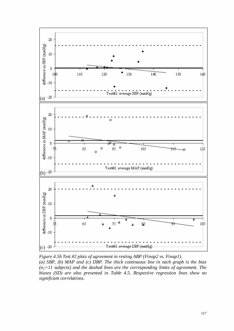
117
Figure 4.5b Test #2 plots of agreement in resting ABP (Finap2 vs. Finap1).
(a) SBP, (b) MAP and (c) DBP. The thick continuous line in each graph is the bias
(n2=11 subjects) and the dashed lines are the corresponding limits of agreement. The
biases (SD) are also presented in Table 4.5. Respective regression lines show no significant correlations.
(a)
(b)
(c)
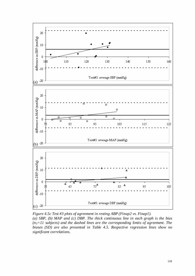
118
Figure 4.5c Test #3 plots of agreement in resting ABP (Finap2 vs. Finap1).
(a) SBP, (b) MAP and (c) DBP. The thick continuous line in each graph is the bias (n3=11 subjects) and the dashed lines are the corresponding limits of agreement. The
biases (SD) are also presented in Table 4.5. Respective regression lines show no
significant correlations.
(a)
(b)
(c)
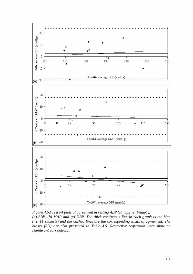
119
Figure 4.5d Test #4 plots of agreement in resting ABP (Finap2 vs. Finap1).
(a) SBP, (b) MAP and (c) DBP. The thick continuous line in each graph is the bias
(n4=11 subjects) and the dashed lines are the corresponding limits of agreement. The
biases (SD) are also presented in Table 4.5. Respective regression lines show no significant correlations.
(a)
(b)
(c)

120
Table 4.5 Bias (SD) in resting ABP (Finap2 vs. Finap1). Bias (SD) computed for SBP, MAP and DBP. They are also plotted in Figures 4.5(a-d).
Tests #1 to #4 were assessed separately (i.e. n1=n2=n3=n4=11 subjects) because the
null hypothesis was rejected.
Test # SBP MAP DBP
mean SD mean SD mean SD
1 7.6 6.82 6.0 4.43 5.4 4.67
2 0.3 7.87 1.8 8.25 1.5 9.25
3 6.3 7.80 3.4 5.25 1.9 4.78
4 2.4 10.67 2.0 7.87 1.7 7.43
Table 4.6 Mean (SD) of RMSE in resting ABP (Finap2 vs. Finap1).
Mean (SD) computed for SBP, MAP and DBP. Tests #1 to #4 were assessed separately
(i.e. n1=n2=n3=n4=11 subjects) because the null hypothesis was rejected.
Test # SBP MAP DBP
mean SD mean SD mean SD
1 9.0 4.71 6.4 3.87 6.0 3.86
2 6.0 5.02 5.4 6.36 6.2 6.83
3 8.2 6.05 4.2 4.80 3.4 3.87
4 9.3 5.28 6.6 4.42 6.2 4.21

121
4.3.2.2 Resting ABP: Bandwidth
ANOVA results with p-values (2 ways 4 levels design) for 95K and 99K are shown
in Table 4.7. Figure 4.6 shows the plots of means of bandwidth limits for the ‘Finap’
and ‘Test’ main effects. No significant difference was detected for each bandwidth
limit. Hence, the respective results were pooled (n=44). For 95% bandwidth, the mean
(SD) of 95,1FinapK and 95,2FinapK were obtained as 4.6 (0.76) Hz and 4.5 (0.87) Hz
respectively. Similarly, for 99% bandwidth, the mean (SD) of 99,1FinapK and 99,2FinapK
were obtained as 6.5 (0.66) Hz and 6.4 (0.85) Hz respectively.
4.3.2.3 Resting ABP: Frequency Response and Magnitude Squared Coherence
The analysis in section 4.3.2.2 above showed that there were no significant differences
between the measurement devices for the 95% and 99% bandwidths, and the
computation results were pooled. This means that )(ˆ fH and )(ˆ 2 f generated from
individual subjects’ spectral curves can also be pooled. Using Equations 4.5 and 4.6, the
respective average spectral curves are shown in Figure 4.7.
The average gain spectrum shows that the cut-off frequency to -3 dB value is
approximately 13.3 Hz. The average phase spectrum is barely shifted within ±10°. The
average magnitude squared coherence of one is achieved up to approximately 7.0 Hz. It
is maintained to at least 0.5 up to approximately 12.5 Hz, although the error bars are
widening.

122
Table 4.7 ANOVA p-values for the 95% and 99% bandwidth limits. The ANOVA results (2 ways 4 levels design) for „Finap‟ and „Test‟ main effects, and
their interaction. No significant difference was detected for each bandwidth limit.
95% 99%
‘Finap’ effect 0.079 0.387
‘Test’ effect 0.864 0.882
‘Finap’ x ‘Test’ interaction 0.351 0.397
Figure 4.6 Plots of means of bandwidth limits for ABP pulses. (a) „Finap‟ main effect; (b) „Test‟ main effect. The effects were plotted for 95% (cross)
and 99% (triangle) bandwidth limits. The error bars are ±1SD of the respective means.
(a)
(b)
Mea
ns
of
ban
dw
idth
lim
its
(H
z)
Mea
ns
of
ban
dw
idth
lim
its
(H
z)

123
Figure 4.7 Spectral curves between ABP measurements with two Finapreses.
(a) Average gain spectrum: the -3 dB point occurs at approximately 13.3 Hz (dotted
lines); (b) average phase spectrum remains stable even beyond 15 Hz; (c) average magnitude squared coherence remains above 0.5 up to about 12.5 Hz (dotted lines). The
computation was from pooled results (n=44 measurements). The error bars are ±1SD
for respective frequencies.
(a)
(b)
(c)

124
4.3.2.4 Resting ABP: Assessment of Drift
ANOVA results with p-values (2 ways 4 levels design) for the are shown in Table
4.8. Figure 4.8 shows the plots of means of percentage change for the ‘Finap’ and ‘Test’
main effects. No significant differences were obtained for SBP, MAP and DBP. Hence,
the respective results were pooled (n=44). The mean (SD) of ΨFinap1, ΨFinap2 and
were computed for SBP, MAP and DBP. The results are:
ΨFinap1 : -0.3 (6.55), -0.7 (4.31) and -1.0 (4.99) %
ΨFinap2 : 1.1 (5.86), -0.1 (4.80) and -0.3 (5.75) %
: 1.4 (7.66), 0.6 (5.62) and 0.7 (7.01) %
The plots of agreement for SBP, MAP and DBP are shown in Figure 4.9. The
regression lines produced no significant correlations.
4.3.2.5 ABP Dynamic Change: Valsalva Manoeuvre
ANOVA results with p-values (2 ways 4 levels design) for the VM are shown in
Table 4.9. Figure 4.10 shows the plots of means of percentage change for the ‘Finap’
and ‘Test’ main effects. No significant differences were obtained for SBP, MAP and
DBP. Hence, the respective results were pooled (n=44). The mean (SD) of ΦFinap1,VM,
ΦFinap2,VM and VM were computed for SBP, MAP and DBP. The results are:
ΦFinap1,VM : 11.56 (9.75), 10.15 (7.28) and 9.97 (6.72) %
ΦFinap2,VM : 12.02 (9.51), 10.60 (7.34) and 10.04 (6.73) %
VM : 0.46 (2.35), 0.45 (2.37) and 0.08 (2.21) %
The plots of VM agreement for SBP, MAP and DBP are shown in Figure 4.11. The
regression lines produced no significant correlations.

125
Table 4.8 ANOVA p-values for the assessment of drift. The ANOVA results (2 ways 4 levels design) for the „Finap‟ and „Test‟ main effects, and
their interaction for SBP, MAP and DBP. No significant differences were detected.
SBP MAP DBP
‘Finap’ effect 0.429 0.594 0.603
‘Test’ effect 0.670 0.905 0.916
‘Finap’ x ‘Test’ interaction 0.056 0.075 0.108
Figure 4.8 Plots of means of percentage change in the assessment of ABP drift.
(a) „Finap‟ main effect; (b) „Test‟ main effect. The effects were plotted for SBP
(diamond), MAP (square) and DBP (triangle). The graphs are slightly shifted from each other to avoid superposition of the error bars. The error bars are ±1SD of the
respective means.
(a)
(b)
Mea
ns
of
per
cen
tag
e ch
ang
e (%
) M
ean
s o
f p
erce
nta
ge
chan
ge
(%)
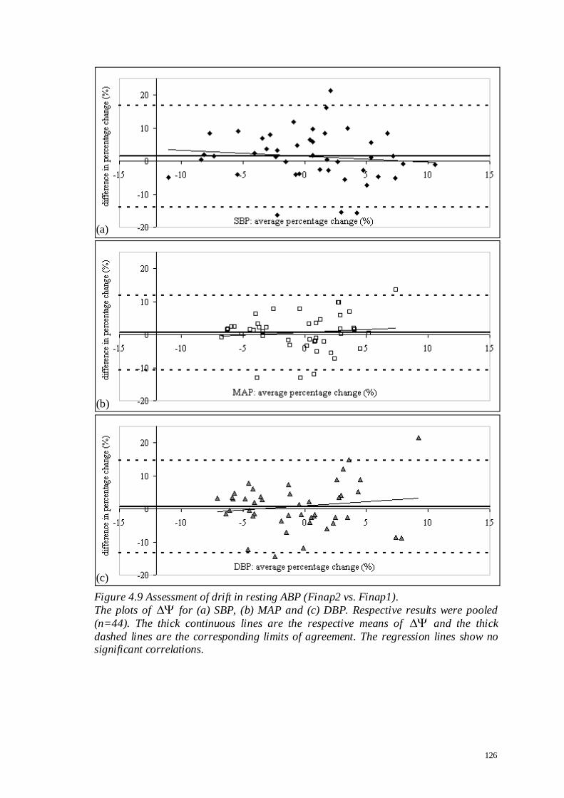
126
Figure 4.9 Assessment of drift in resting ABP (Finap2 vs. Finap1).
The plots of for (a) SBP, (b) MAP and (c) DBP. Respective results were pooled
(n=44). The thick continuous lines are the respective means of and the thick
dashed lines are the corresponding limits of agreement. The regression lines show no significant correlations.
(a)
(b)
(c)

127
Table 4.9 ANOVA p-values for VM during Valsalva manoeuvre.
The ANOVA results (2 ways 4 levels design) „Finap‟ and „Test‟ main effects, and their
interaction for SBP, MAP and DBP. No significant differences were detected.
SBP MAP DBP
‘Finap’ effect 0.233 0.142 0.794
‘Test’ effect 0.586 0.843 0.976
‘Finap’ x ‘Test’ interaction 0.337 0.094 0.160
Figure 4.10 Plots of means of ABP percentage change during Valsalva manoeuvre.
(a) „Finap‟ main effect; (b) „Test‟ main effect. The effects were plotted for SBP
(diamond), MAP (square) and DBP (triangle). The graphs are slightly shifted from each other to avoid superposition of the error bars. The error bars are ±1SD of the
respective means.
(a)
(b)
Mea
ns
of
per
cen
tag
e ch
ang
e (%
) M
ean
s o
f p
erce
nta
ge
chan
ge
(%)

128
Figure 4.11 ABP dynamic change during Valsalva manoeuvre (Finap2 vs. Finap1).
The plots of VM for (a) SBP, (b) MAP and (c) DBP. Respective results were pooled
(n=44). The thick continuous lines are the respective means of VM and the thick
dashed lines are the corresponding limits of agreement. The differences are well
scattered with no significant correlations.
(a)
(b)
(c)

129
4.4 Comparative Study of STAbp and Finapres
The comparative study between two Finapreses in the previous section demonstrated
that there are differences between simultaneous ABP measurements even though they
were monitored with devices of the same specifications and model number. The
differences will be compared further in section 4.5. Before that, the STAbp prototype
(device B) was evaluated against the Finapres (device A). Finap1 was again used as
reference. Measurement protocols were very similar to the previous study. As
mentioned in section 4.2, this is to enable direct comparisons of results between both
studies and to interpret the differences accordingly.
4.4.1 Method
19 subjects were recruited for this study (10 males, 9 females, age (mean ± SD) 34 ± 12
years). The participants were all staff from the Medical Physics department. Written
consent was given by each participant prior to the arrangement for the ABP
measurements. The study was approved by the Leicestershire ethics committee
(reference number: 4680).
To prepare the subject for the experiment, each subject was asked to sit comfortably
upright on a chair with back support. The room temperature was maintained at
approximately 22 ºC. The right STA was first located by palpation. After that, the head
frame of the STAbp was fixed with four padded brackets fastened against the scalp. The
padded brackets were equally spaced around the head. This was followed by placing the
front end of the probe on the skin with the underlying STA. The probe placement was

130
then fixed by its fastening bracket against the head frame. The probe and head frame
were described in sections 3.3.1 and 3.3.2 respectively.
For the finger ABP measurement, an appropriate Finapres cuff was selected and fitted
onto the right middle finger of the subject. The hand rested on the right lap of the
subject. The height difference between the STA and the finger artery was measured.
This is to offset the hydrostatic pressure difference between the ABP in the finger artery
and the STA. The hydrostatic pressure difference for each centimeter difference in
height was taken as P = h. .g = (0.01 x 1060 x 9.81) x 750 / (1 x 10⁵) = 0.77
mmHg/cm where h is the height difference (in m), is the blood density (in kg/m3)
and g is the acceleration due to gravity (in ms-2). This equation does not take into
account individual values of blood density across the sample population.
When the setup of the experiment was complete, both recorders were switched on to
monitor the ABP for several minutes. The subject was asked to relax and breathe
normally during measurements. When the waveforms were stable, the self-calibration
facilities in both devices were then temporarily switched off. The self-calibration
algorithm in the STAbp was described in section 3.3.7. The paired resting ABP
waveforms were recorded for 3 min.
After the 3 min recording, the respective self-calibration facilities in both measurement
devices were re-enabled for several minutes. Both self-calibration facilities were then
again temporarily switched off to carry out the IHG exercise.

131
During the IHG exercise, each subject was asked to squeeze a rolled-up slightly inflated
sphygmomanometer cuff at 30% maximal voluntary compression for 2 min (Panerai et
al., 2001). The compression on the cuff was monitored with an aneroid pressure gauge.
After 2 min, the subject would release the grip suddenly. A dynamic mean ABP drop
was expected. The recording of the ABP waveforms continued for another 1 min before
the measurements were terminated in both devices.
From the resting ABP recording, 16 cardiac pulses at the beginning and 16 cardiac
pulses towards the end of the 3 min recording were retrieved. The analysis techniques
for these ranges of waveforms were described in sections 4.2.1 to 4.2.4. The recorded
waveforms during the IHG exercise was analysed with the technique described in
section 4.2.5. For each parameter considered, the null hypothesis states that there is no
statistical significance between mean values. Paired t-tests were carried out to test this
hypothesis.
4.4.2 Results
In paired ABP recordings from 19 subjects, both ABP waveforms from the STAbp and
Finap1 were visually checked to determine if their quality was satisfactory. Using this
exclusion criterion, all recordings with Finap1 were satisfactory. For resting ABP
recordings, one subject was excluded as the ABP waveshape measured with the STAbp
was very poor. Another two subjects were also excluded. This was because the Setpt
determined by the self-calibration facility in the STAbp did not lead to physiologically
meaningful ABP waveforms. These will be further discussed in section 4.6. Hence, the
remaining 16 subjects’ recordings were analysed by the techniques described in sections

132
4.2.1 to 4.2.4. The self-calibration algorithm to determine the Setpt was described in
section 3.3.7.
For the assessment of ABP dynamic change during IHG exercise, the same three
subjects above were excluded. Another two subjects’ recordings by STAbp were also
excluded due to poor ABP waveforms. These will be further discussed in section 4.6.
Hence, the remaining 14 subjects’ recordings were analysed based on the technique
described in section 4.2.5.
The presentation of analysis results follows the sequence described in section 4.2 and
adopts the same headings. Figure 4.12 shows an example of the paired resting ABP
recordings for 16 cardiac pulses at the beginning and 16 cardiac pulses towards the end
of the 3 min recording respectively. The former waveform segment was analysed
according to the first three data analysis techniques described in sections 4.2.1 to 4.2.3.
Both waveform segments were then analysed for the assessment of drift according to
the technique described in section 4.2.4. Lastly, the analysis technique described in
section 4.2.5 was used for the assessment of the ABP dynamic change during IHG
exercise. An example recording is shown with its beat-to-beat SBP, MAP and DBP in
Figure 4.13.

133
Figure 4.12 Resting ABP waveforms (STAbp vs. Finap1).
Example of 16 cardiac pulses at the beginning (a) and 16 cardiac pulses towards the end (b) of a 3 min recording with STAbp (black continuous line) and Finap1 (grey
dashed line). Finap1 was used as reference.
(a)
(b)

134
Figure 4.13 SBP, MAP and DBP during IHG exercise. The beat-to-beat ABP with STAbp (black continuous lines) and Finap1 (grey dashed
lines) are shown for SBP (diamond), MAP (square) and DBP (triangle). The vertical
lines indicate the beginning and end of the 2 min IHG exercise. When the hand grip was
released at the end of the 2 min, a clear dynamic drop in ABP can be observed (as indicated by asterisks).

135
4.4.2.1 Resting ABP: Agreement
The plots of agreement are shown in Figure 4.14 for SBP, MAP and DBP respectively.
The bias (SD) for SBP, MAP and DBP were computed as -23.1 (15.05), -10.8 (13.83)
and -12.4 (12.93) mmHg. Similarly, the corresponding mean (SD) of RMSE were
obtained as 23.5 (14.56), 13.6 (10.90) and 13.6 (11.65) mmHg respectively. Paired t-
tests showed significant differences for SBP, MAP and DBP (p<0.001, p<0.01 and
p<0.01 respectively). Hence, the null hypothesis was rejected.
Figure 4.14 also included regression lines. Significant correlations were obtained. The
correlation coefficients were 0.61 (p<0.02), 0.75 (p<0.01) and 0.69 (p<0.01) for SBP,
MAP and DBP respectively. No significant correlation was detected between subjects’
ABP differences with age.
4.4.2.2 Resting ABP: Bandwidth
For the 95% bandwidth limit, the mean (SD) of 95,STAbpK and 95,1FinapK were computed
as 3.2 (1.10) Hz and 4.8 (0.88) Hz respectively. Paired t-test showed statistical
significance for 95K (p<0.001). Similarly, for the 99% bandwidth limit, the mean (SD)
of 99,STAbpK and 99,1FinapK were computed as 5.3 (1.46) Hz and 6.8 (0.73) Hz
respectively. Paired t-test showed statistical significance for 99K (p<0.01).
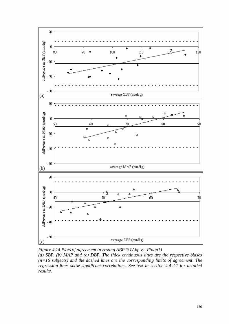
136
Figure 4.14 Plots of agreement in resting ABP (STAbp vs. Finap1). (a) SBP, (b) MAP and (c) DBP. The thick continuous lines are the respective biases
(n=16 subjects) and the dashed lines are the corresponding limits of agreement. The
regression lines show significant correlations. See text in section 4.4.2.1 for detailed
results.
(a)
(b)
(c)

137
4.4.2.3 Resting ABP: Frequency Response and Magnitude Squared Coherence
Figure 4.15 shows the )(ˆ fH and )(ˆ 2 f spectral curves (Equations 4.5 and 4.6). The
cut-off frequency (-3 dB point) of the average gain spectrum is approximately 3 Hz.
There is very little phase shift in the average phase spectrum until about 3.2 Hz when it
gradually increases before stabilizing from approximately 9.5 Hz. The average
coherence spectrum shows that the coherence is high, remaining above 0.5 even beyond
12 Hz.
4.4.2.4 Resting ABP: Assessment of Drift
The mean (SD) of ΨFinap1, ΨSTAbp and were computed for SBP, MAP and DBP. The
results are:
ΨFinap1 : -0.8 (6.43), -1.5 (6.00) and -2.2 (6.60) %
ΨSTAbp : 1.0 (7.16), 0.9 (7.79) and -0.1 (9.00) %
: 1.8 (5.64), 2.3 (5.23) and 2.2 (6.52) %
The plots of for SBP, MAP and DBP are shown in Figure 4.16. are well
scattered with no significant correlations. Paired t-tests also showed no significant
differences.
4.4.2.5 ABP Dynamic Change: IHG Exercise
An example of the paired ABP during IHG exercise is shown in Figure 4.13 with the
beat-to-beat SBP, MAP and DBP. The dynamic drop of the ABP after the release of the
handgrip is indicated by asterisks. The mean (SD) of ΨFinap1,IHG, ΨSTAbp,IHG and IHG
were computed for SBP, MAP and DBP. The results are:
ΦFinap1,IHG : 10.5 (11.81), 14.1 (12.34) and 15.8 (14.20) %
ΦSTAbp,IHG : 10.3 (9.69), 11.8 (10.45) and 11.3 (11.21) %

138
IHG : -0.2 (10.04), -2.3 (9.49) and -4.5 (11.66) %
The plots of IHG for SBP, MAP and DBP between STAbp and Finap1 are shown in
Figure 4.17. IHG are well scattered with no significant correlations. Paired t-tests
also showed no significant differences.

139
Figure 4.15 Spectral characteristic curves (STAbp vs. Finap1).
(a) Average gain spectrum: the cut-off frequency at -3 dB is approximately 3 Hz (dotted
lines); (b) average phase spectrum remains fairly stable up to about 3.2 Hz and gradually increases before stabilising at approximately 9.5 Hz (dotted lines); (c)
average magnitude squared coherence remains above 0.5 even beyond 12 Hz (dotted
lines). The error bars are ±1SD for respective frequencies (n=16 subjects).
(a)
(b)
(c)

140
Figure 4.16 Assessment of drift in resting ABP (STAbp vs. Finap1).
The plots of for (a) SBP, (b) MAP and (c) DBP (n=16 subjects). The thick continuous lines are the respective means of and the thick dashed lines are the
corresponding limits of agreement. The regression lines show no significant
correlations.
(a)
(b)
(c)

141
Figure 4.17 ABP dynamic change during IHG exercise (STAbp vs. Finap1).
The plots of IHG for (a) SBP, (b) MAP and (c) DBP. The thick continuous lines are
the respective means of IHG (n=14 subjects) and the dashed lines are the
corresponding limits of agreement. The regression lines show no significant
correlations.
(a)
(b)
(c)
142
4.5 Inter-Study Comparisons
Two separate comparative studies (sections 4.3 and 4.4) were performed and the ABP
waveforms were analysed according to standard statistical methods (section 4.2). The
analysis results from both comparative studies are summarized in Table 4.10, tabulated
in two pages. The left column are results for comparative study between two
Finapreses, whereas, the right column are results for comparative study of STAbp and
Finap1. Results of the four parameters described in section 4.2 are presented in this
table, whereas the comparisons of spectral responses (section 4.2.3) are presented in
Figure 4.18.
Despite the potential influence of different measurement sites, to be discussed later,
further comparison between the two separate studies would be useful to highlight areas
of significant differences. Independent t-tests were carried out for the agreement of ABP
(SBP, MAP and DBP), 95% and 99% bandwidth limits and the assessment of ABP drift
(SBP, MAP and DBP). Statistical results with significant p-values are shown in Table
4.11. The results of ABP dynamic change due to activity were not further compared as
different activities were carried out (i.e. Valsalva manoeuvre or IHG exercise).
In the inter-study comparisons of ABP agreement, only Tests #1 and #3 (Table 4.11)
were compared with the comparative study of STAbp and Finap1 because the same
finger was measured by Finap1 in all the three experiments, i.e. the right middle finger
(Table 4.1). In theory, Bonferroni correction would be needed for these multiple
comparisons (Bland, 1995; Campbell and Machin, 1995), but given the very small p-
values obtained, it does not make a difference.

143
Inter-study comparisons of the 95% and 99% bandwidth limits only apply to the STAbp
and Finap2 as both studies used Finap1 as reference. Significant differences were
obtained for both bandwidth limits (Table 4.11). Next, the inter-study comparisons of
the assessment of ABP drift produced no significant differences for SBP, MAP and
DBP.
The spectral curves of Figures 4.7 and 4.15 are replotted in Figure 4.18 to further
compare the curves between both studies. In the average gain spectrum, the cut-off
frequency at -3 dB apparently dropped from approximately 13.3 Hz to 3 Hz. However,
comparisons of the two curves show that STAbp gain response seems to recover at
higher frequencies suggesting that it should be possible to recover a flat response with
further modifications in hardware and/or software.
The average phase spectrum in STAbp vs. Finap1 remained fairly stable until about 3.2
Hz and gradually increased before stabilising at approximately 9.5 Hz (indicated by
dotted lines). The phase shift is increasingly leading from 0º to 110º within the
frequency range 3.2 Hz and 9.5 Hz. However, between two Finapreses, the average
phase shift remained stable even beyond 15 Hz. Lastly, the average magnitude squared
coherence remained above 0.5 even beyond 12.5 Hz for both studies. Further discussion
and interpretation of these curves will be presented in the next section.

144
Table 4.10 Summary of results from both comparative studies. Only significant p-values are listed.
Section 4.3: Finap2 vs. Finap1 Section 4.4: STAbp vs. Finap1
4.3.2.1 Resting ABP: Agreement 4.4.2.1 Resting ABP: Agreement
Bias (SD)
[mmHg]
Mean (SD)
of RMSE
[mmHg]
Bias (SD)
[mmHg]
Mean (SD)
of RMSE
[mmHg]
Test #1
SBP 7.6 (6.82) 9.0 (4.71) SBP -23.1 (15.05) see †a 23.5 (14.56)
MAP 6.0 (4.43) 6.4 (3.87) MAP -10.8 (13.83) see †b 13.6 (10.90)
DBP 5.4 (4.67) 6.0 (3.86) DBP -12.4 (12.93) see †c 13.6 (11.65)
Test #2
SBP 0.3 (7.87) 6.0 (5.02) Paired t-test
MAP 1.8 (8.25) 5.4 (6.36) †a p<0.001
DBP 1.5 (9.25) 6.2 (6.83) †b p<0.01
Test #3 †c p<0.01
SBP 6.3 (7.80) 8.2 (6.05)
MAP 3.4 (5.25) 4.2 (4.80) Correlation coefficient
DBP 1.9 (4.78) 3.4 (3.87) †a 0.61 (p<0.02)
Test #4 †b 0.75 (p<0.01)
SBP 2.4 (10.67) 9.3 (5.28) †c 0.69 (p<0.01)
MAP 2.0 (7.87) 6.6 (4.42)
DBP 1.7 (7.43) 6.2 (4.21)
4.3.2.2 Resting ABP: Bandwidth 4.4.2.2 Resting ABP: Bandwidth
Mean (SD)
[mmHg] 95% 99% Mean (SD)
[mmHg] 95% 99%
Finap1 4.6 (0.76) 6.5 (0.66) Finap1 4.8 (0.88) 6.8 (0.73)
Finap2 4.5 (0.87) 6.4 (0.85) STAbp 3.2 (1.10) 5.3 (1.46)
Paired t-test p<0.001 p<0.01
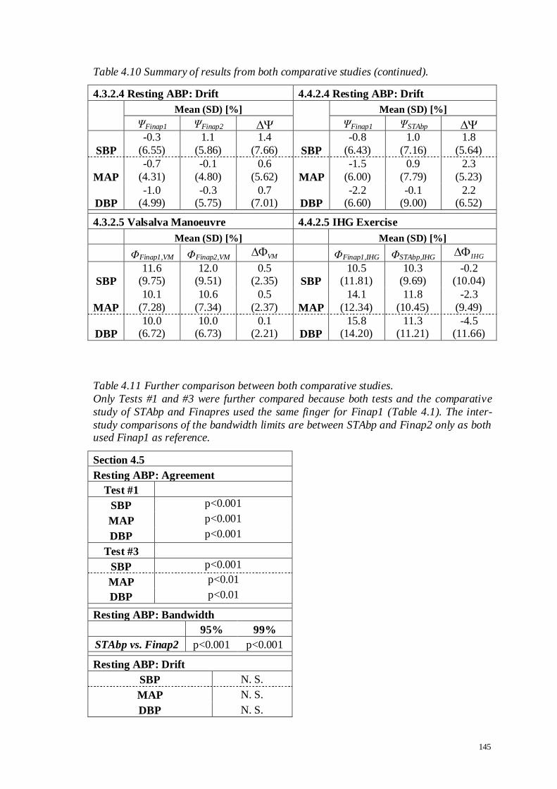
145
Table 4.10 Summary of results from both comparative studies (continued).
4.3.2.4 Resting ABP: Drift 4.4.2.4 Resting ABP: Drift
Mean (SD) [%]
Mean (SD) [%]
ΨFinap1 ΨFinap2 ΨFinap1 ΨSTAbp
SBP
-0.3
(6.55)
1.1
(5.86)
1.4
(7.66) SBP
-0.8
(6.43)
1.0
(7.16)
1.8
(5.64)
MAP
-0.7
(4.31)
-0.1
(4.80)
0.6
(5.62) MAP
-1.5
(6.00)
0.9
(7.79)
2.3
(5.23)
DBP
-1.0 (4.99)
-0.3 (5.75)
0.7 (7.01) DBP
-2.2 (6.60)
-0.1 (9.00)
2.2 (6.52)
4.3.2.5 Valsalva Manoeuvre 4.4.2.5 IHG Exercise
Mean (SD) [%] Mean (SD) [%]
ΦFinap1,VM ΦFinap2,VM VM ΦFinap1,IHG ΦSTAbp,IHG IHG
SBP
11.6 (9.75)
12.0 (9.51)
0.5 (2.35) SBP
10.5 (11.81)
10.3 (9.69)
-0.2 (10.04)
MAP
10.1
(7.28)
10.6
(7.34)
0.5
(2.37) MAP
14.1
(12.34)
11.8
(10.45)
-2.3
(9.49)
DBP
10.0 (6.72)
10.0 (6.73)
0.1 (2.21) DBP
15.8 (14.20)
11.3 (11.21)
-4.5 (11.66)
Table 4.11 Further comparison between both comparative studies.
Only Tests #1 and #3 were further compared because both tests and the comparative
study of STAbp and Finapres used the same finger for Finap1 (Table 4.1). The inter-
study comparisons of the bandwidth limits are between STAbp and Finap2 only as both used Finap1 as reference.
Section 4.5
Resting ABP: Agreement
Test #1
SBP p<0.001
MAP p<0.001
DBP p<0.001
Test #3
SBP p<0.001
MAP p<0.01
DBP p<0.01
Resting ABP: Bandwidth
95% 99%
STAbp vs. Finap2 p<0.001 p<0.001
Resting ABP: Drift
SBP N. S.
MAP N. S.
DBP N. S.

146
Figure 4.18 Comparison of spectral responses between both studies. Spectral curves from comparison study between two Finapreses (grey continuous lines)
and comparative study of STAbp and Finapres (black continuous lines). They are
replotted from Figures 4.7 and 4.15. (a) Average gain spectrum with the cut-off
frequency at -3 dB indicated by dotted lines; (b) average phase spectrum, see text in section 4.5 for detailed description; (c) average magnitude squared coherence remains
above 0.5 even beyond 12.5 Hz for both curves (indicated by dotted lines). The graphs
are slightly shifted from each other to avoid superposition of the error bars. The error
bars are the respective ±1SD at each frequency value.
(a)
(b)
(c)

147
4.6 Discussion
To simplify the following text, Study1 refers to the comparative study between two
Finapreses, and Study2 refers to the comparative study of STAbp and Finapres.
Both Study1 and Study2 are original contributions of this thesis. Evaluations of the
Finapres against intravascular measurements were reported by a number of authors
using different measurement sites, e.g. brachial, radial or ascending aorta (Epstein et al.,
1991; Farquhar, 1991; Imholz et al., 1998; Omboni et al., 1993; Pace and East, 1991;
van Egmond et al., 1985). For the objectives of this chapter, these reported results are
not directly applicable. Instead, Study1 demonstrated the inherent differences of
simultaneous ABP measurements by two Finapreses of the same model (Table 4.10).
The information generated is useful to gauge the results from Study2.
The following subsections begin with further discussion regarding exclusion of several
subjects’ recordings from analysis. This is followed by discussion of main findings from
both comparative studies. Next, potential causes of differences in ABP measurements in
both comparative studies are listed, and limitations of the comparative studies are
identified. Finally, the follow up of safety evaluation of the STAbp device from section
3.4.2 and suggestions for future work are presented.
4.6.1 Recordings Excluded from Analysis
Resting ABP recordings
In Study2, three subjects’ paired resting ABP recordings were excluded for analysis. In
two of them, the Setpt determined with the self-calibration algorithm in the STAbp did

148
not lead to meaningful ABP waveform. Figure 4.19 shows an example. With increasing
compressing pressure, the PPG baseline remained at a similar level. The span of the
compressing pressures in this example is approximately 70 mmHg. This phenomenon
may be due to insufficient compression from the inflatable sealed air chamber on the
tissue covering the STA. It may also be due to thick and/or stiff skin tissue that
attenuates the pressure transmission from the chamber to the STA. In comparison,
Figure 3.9 shows a typical PPG waveform with the PPG baseline gradually increasing
with compressing pressure.
In another subject, meaningful ABP waveform monitored by the STAbp could not be
obtained. The morphology of the ABP waveform was very poor. The PPG pulse
amplitude was small, which may suggest weak arterial pulse. This was verified by
palpation. However, simultaneous recording by Finap1 in the finger showed good
quality ABP waveform. This may also suggest that the STA is embedded deep below
the skin surface. The implication of this for clinical practice is that in some subjects
with weak arterial pulse or low ABP, the STAbp device may struggle to monitor ABP in
the STA.
ABP recordings during IHG exercise
Five subjects’ recordings during the IHG exercise were excluded. Three of the subjects
are the same as the subjects mentioned above. Recordings from another two subjects
were excluded due to poor quality ABP waveforms in the STAbp. Further attempts with
these two subjects did not produce satisfactory ABP waveforms. The precise reasons
behind this problem could not be identified at the time. Technical limitations of the
STAbp device may not be the cause of the poor quality waveform as the resting ABP

149
recordings from these subjects were satisfactory and accepted for analysis. Thus, other
possible causes were considered. For instance, the artery may have been shifted away
from its initial position after prolonged compression during resting ABP recording; it
may also be possible that the tissue and the artery required time to recover to its initial
state after prolonged compression.
Atypical PPG waveform
In one subject (different from those mentioned above), an atypical PPG with inverted
waveform was observed during resting ABP recording (Figure 4.20(a)). This is different
from the typical PPG shown in Figure 4.20(b). In theory, the PPG decreases as the
arterial blood volume increases, and vice versa (section 2.5.2). To overcome this
problem, the placement of the probe was repositioned until a satisfactory PPG was
obtained. At current development, the repositioning approach is subjective. With this
approach, the subsequent ABP recording from this subject was satisfactory and was not
excluded from analysis. Inverted PPG waveforms were also observed in the radial
(Nijboer and Dorlas, 1982) and carotid (Weinmann et al., 1977) arteries. This
contradiction to the theory of in-vivo PPG indicates that other factors are affecting the
generated PPG. Apart from the arterial blood volume, factors that may affect the light
scattering and reflection back to the photodetector include movement of blood vessel
walls, orientation of red blood cells (Allen, 2007), bone (Näslund et al., 2006) and
venous engorgement (Nijboer and Dorlas, 1982). However, these studies were not based
on the in-vivo STA and its surrounding tissue. The occurrence of atypical PPG
waveforms does pose a technical concern for accurate and reliable ABP measurements
based on volume clamping technique with photoplethysmography. Further investigation
is needed to clarify the origin of these atypical inverted PPG waveforms.

150
Figure 4.19 PPG with fairly constant baseline.
The waveforms were recorded by the STAbp. (a) The external compressing pressure is
increased in steps of 5 mmHg/s; (b) the corresponding PPG baseline barely changes in a span of approximately 70mmHg (indicated within two vertical dashed lines).
Figure 4.20 Atypical vs. typical PPG waveforms.
(a) An example of an atypical PPG with inverted waveshape; (b) An example of a
typical PPG waveform.
(a)
(b)
(a) (b)

151
4.6.2 Main Findings
Analysis result for the ABP agreement in Study1 shows that the paired measurements
from four combinations of fingers did not allow the measurement results to be pooled,
due to significant differences between tests (Tables 4.2 to 4.4). Furthermore, Figure
4.18 demonstrated that the frequency gain response was only achieved up to 13.3 Hz
and the coherence (≥0.5) was only achieved up to 12.5 Hz. These findings give some
indication of what could be expected from Study2.
Resting ABP: agreement
In Study1, Tables 4.2 to 4.4 show that all the significant p-values are related to ‘Finap2
Test #1’ (labelled as 5 ). Definite causes are unclear. There was no significant
correlation between the ABP differences and age of the subjects. Thus, it may be due to
inappropriate cuff fitting (i.e. too loose or too tight), poorer blood circulation in one
finger during ABP measurements, or possibly compression of the fingers as the subject
may be leaning forward or backward during ABP measurements.
In Study2, the significant p-values for the ABP agreement (Table 4.10) could be due to
several key factors. First, the ABP were recorded from two different measurement sites.
Referring to Figure 1.2, the SBP tends to be raised in the periphery in younger subjects
which may also explain the reason a larger bias in SBP was obtained than the MAP and
DBP. The differences in physiological condition in different measurement sites may
also have contributed to the differences in ABP measurements. The clinical
interpretation regarding the significance of the ABP differences between measurement
devices could depend on an individual’s baseline ABP. For instance, a person who is
already diagnosed with hypertension may require further treatment if the measured ABP

152
is close to the ABP threshold for hypertension, i.e. approximately 140/90 mmHg
(O'Brien et al., 2003). For individuals within the healthy ABP range, i.e. generally
considered as 120/80 mmHg, these differences may not cause clinical concerns.
Second, the area of compression by the inflatable sealed air chamber in the probe may
not have been optimised in order for the ABP to be measured accurately. Third, the
fixing of the head frame against the scalp may not be adequate, which leads to
movement as the compressing pressure is continuously adjusted when the ABP is
continuously monitored. Fourth, the effectiveness of the pressure transmission at
different compressing pressures from the inflatable sealed air chamber in the probe to
the STA may not be linear. As the compressing pressure is modulated during ABP
monitoring, the STA may not have been compressed sufficiently by the inflatable sealed
air chamber which led to a lower ABP measurement values in comparison with Finap1.
Resting ABP: bandwidth
The 95% and 99% bandwidth limits of the STAbp recording were both significantly
lower than those recorded by Finap1 (Table 4.10). This may be due to a limitation of
the STAbp hardware to measure the ABP to achieve better agreement with Finap1.
Having said that, the significant differences may suggest that pulse wave propagation
and reflection, differences in local blood flow regulation, vasomotor tone and arterial
elasticity play a part in changing the ABP waveshape that increases the frequency
content of the peripheral ABP pulses.
Resting ABP: frequency response and magnitude squared coherence
In the comparison of both gain spectrum curves, there is a drop in gain in Study2
between 1.5 Hz and 10 Hz before it shows gain of approximately the same as the gain in

153
Study1. Similar to the reason given above, the drop in gain may be due to limitation of
the STAbp hardware. Another possible explanation is that the averaged gain spectra
were computed from measurements in subjects of wide age range. As shown in Figure
1.2 (section 1.1), qualitative comparison between central and peripheral ABP
waveshape and amplitude in young subjects show considerable differences; whereas the
differences of the ABP waveshape and amplitude are less obvious in older subjects.
Figure 4.18 shows an increase of phase leading between 3.2 Hz and 9.5 Hz in Study2.
This again, may be related to the limitation of the test equipment in terms of sufficient
frequency response to produce ABP waveform with better agreement when compared
against the ABP measured by Finap1. Having said that, the phase shift in the spectral
curve is not surprising due to the influence of pulse wave propagation and reflection in
different arteries. As mentioned in section 1.1, in comparison with more central ABP
waveform, peripheral ABP waveforms in young individuals with more elastic vessel
walls tend to produce delayed systolic peak. However, the frequency range that this
phase difference should occur is uncertain.
The magnitude squared coherences in both curves (Figure 4.18) were fairly close to one
up to approximately 7.0 Hz. Although the coherences continue to remain above 0.5
beyond 7.0 Hz, the error bars are beginning to widen. This suggests that the evaluation
of ABP waveforms in the frequency domain with the Finapres as reference could be
considered less reliable in frequencies above 7.0 Hz.
Resting ABP: assessment of drift
The results in the assessment of ABP drift need to be interpreted with caution. Non-zero
values (Table 4.10) can only be considered as a drift in ABP measurements by the

154
test device if two key assumptions were made. First, there is no measurement drift in the
reference device Finap1. Second, differences in local physiological conditions are
negligible (e.g. local blood flow regulation, vasomotor tone and arterial elasticity).
Nevertheless, the assessment of drift is a useful evaluation parameter to ensure that
good quality ABP waveforms are obtained. No significant differences were obtained in
the assessment of drift between Study1 and Study2 (Table 4.11). This may suggest that
STAbp is at least as stable as the Finapres for recordings lasting 3 to 4 min.
Sample size
Sample size was somewhat tentative due to unknown SD for various parameters, as well
as initial objective of obtaining descriptive values for some of the parameters such as
frequency response and bandwidth. Due to these reasons, statistical power analysis was
not carried out a priori. However, retrospective calculation based on the sample SD
obtained can be useful for designing future studies. Referring to Table 4.10, a single
calculation of sample size is not possible for all the different parameters described.
Consequently, they would need to be calculated separately. As an example, to detect a
difference of 5 mmHg (O'Brien and Atkins, 1994) for the MAP in STAbp using the
estimated value of SD = 13.83 mmHg (Table 4.10), with 80% power at 0.05 level of
significance for paired data (Campbell and Machin, 1995), the computed sample size
would be 60. The same principle can be applied to other parameters. The difference
between this estimated sample size and the actual number of subjects involved in Study2
is not critical because the null hypothesis was rejected for differences that were greater
than 5 mmHg.

155
4.6.3 Potential Causes of Measurement Differences
Although both STAbp and Finapres operate based on the volume clamping technique
with photoplethysmography, the inherent differences in measurement sites and
recording devices could affect measurement results. Hence, when interpreting each
comparative study, these factors need to be taken into consideration.
Factors that may cause the measurement differences between two Finapreses of the
same model include:
anatomical difference between the fingers;
difference in local blood flow regulation;
motion artefacts;
the snugness of each finger cuff fitted on the fingers;
difference in electronic tolerances between measurement devices.
Factors that may cause differences in the measurements between STAbp and Finapres:
anatomical difference of measurement sites;
differences in design of measurement devices, e.g. area of compression,
optoelectronic physical characteristics for tissue illumination and photodetection,
electronics circuitry and signal processing algorithm. The detailed algorithm in the
Finapres is not clear in the literature, most likely due to commercial implications;
difference in frequency response. The frequency response of the Finapres is
unknown, no relevant literature could be found. The frequency response of the
Finapres could not be assessed in-house as appropriate measurement setup is not
available. For this reason, the best approach would probably be a comparison with a
high-fidelity solid-state catheter-tip intravascular measurement of ABP. The

156
frequency response of STAbp was limited to the block G3 (regulated compressing
pressure), as described in sections 3.4.1 and 3.5.2;
difference in optical pathways, i.e. reflectance configuration in STAbp but
transmittance configuration in Finapres;
difference in mode of compression, i.e. unidirectional compression in STAbp, but
concentric compression in Finapres. Furthermore, the compression on the STA is
supported by the skull at the temporal region.
pressure transmission through the tissue in the temporal region may be attenuated or
amplified differently as compared to the fingers;
differences in tissue elastic properties, vasomotor tone, local blood flow regulation,
and pulse wave propagation and reflection;
with anastomosis in the extra-cranial circulation (section 2.3.2), there is collateral
blood flow in the STA. However, such vascular network may not be available in the
finger artery. Hence, a variation of ABP in the STA may not show similar variation
in the finger ABP, and vice versa;
sensitivity to ambient temperature change may be greater in the finger artery if the
surrounding temperature is not controlled. Local vasoconstriction may be more
significant in the finger artery (Levick, 2003);
motion artefact. The effect could be larger for the STAbp as the device requires a
more complex hardware design than the Finapres to maintain the placement of the
probe on the STA.
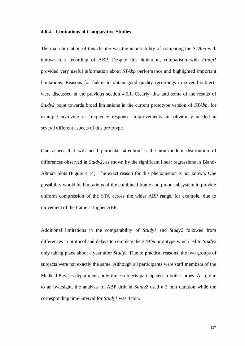
157
4.6.4 Limitations of Comparative Studies
The main limitation of this chapter was the impossibility of comparing the STAbp with
intravascular recording of ABP. Despite this limitation, comparison with Finap1
provided very useful information about STAbp performance and highlighted important
limitations. Reasons for failure to obtain good quality recordings in several subjects
were discussed in the previous section 4.6.1. Clearly, this and some of the results of
Study2 point towards broad limitations in the current prototype version of STAbp, for
example involving its frequency response. Improvements are obviously needed in
several different aspects of this prototype.
One aspect that will need particular attention is the non-random distribution of
differences observed in Study2, as shown by the significant linear regressions in Bland-
Altman plots (Figure 4.14). The exact reason for this phenomenon is not known. One
possibility would be limitations of the combined frame and probe subsystem to provide
uniform compression of the STA across the wider ABP range, for example, due to
movement of the frame at higher ABP.
Additional limitations in the comparability of Study1 and Study2 followed from
differences in protocol and delays to complete the STAbp prototype which led to Study2
only taking place about a year after Study1. Due to practical reasons, the two groups of
subjects were not exactly the same. Although all participants were staff members of the
Medical Physics department, only three subjects participated in both studies. Also, due
to an oversight, the analysis of ABP drift in Study2 used a 3 min duration while the
corresponding time interval for Study1 was 4 min.

158
4.6.5 Safety Evaluation
As a follow up assessment from section 3.4.2 for the safety evaluation of the STAbp
prototype device, two safety issues required reassessment after the comparative study of
STAbp and Finap1. They are reported as follows:
Tissue heating: there was no reported sensation of heating or redness of skin due to
the optoelectronic components in the probe placed close to the skin.
Risk of tissue ischaemia: multiple large and soft paddings fastened around the head
with the head frame provide evenly distributed pressure on the scalp tissue (section
3.3.2). The subjects did not report any signs of headache, dizziness or other
discomfort.
4.6.6 Suggestions for Future Work
One of the key tasks for future work is the validation of STAbp against intravascular
measurements. Nevertheless, prior to that, further improvements or modifications of the
STAbp prototype need to be carried out. One of them is to provide different head frame
designs to accommodate different head sizes to improve placement of the probe on the
skin covering the STA. It is more difficult to fasten the same head frame design in
subjects with smaller head size. Hence, with more choices of head frame sizes, a smaller
head frame will also be lighter and more comfortable for participants. In addition to
this, subjects were sitting upright during the experiment, the head frame needs to be
modified to allow studies with participants in the supine position.

159
Different arrangements of the optoelectronic components relative to STA will need
further review to assess its effect on the quality of the PPG signal, and also the causes
for occurrence of atypical PPG waveforms. In addition to that, further review on the
area of compression from the front end of the probe on the STA will be useful to
optimise the effectiveness of the pressure transmission. The use of mathematical
modelling or a suitable experimental test rig to evaluate these factors may be beneficial.
Upon the evaluation of the STAbp against intravascular measurement, one future task
worth considering is to improve the frequency response of the STAbp to provide a flat
frequency response over the bandwidth of interest. This could be achieved by using a
filter equalisation technique. This would be beneficial to improve the accuracy in the
estimation of central ABP waveforms. These developments would be worth pursuing
once all other hardware and software possibilities have been explored.
Future studies are recommended to include studies for dedicated applications such as
baroreceptor sensitivity, dynamic cerebral autoregulation and autonomic nervous
system assessment (e.g. tilt testing, ABP variability and cold pressor test).

160
4.7 Conclusion
With prior knowledge of the inherent differences in ABP measurements with two
Finapreses, the interpretation of the results in the comparative study of STAbp and
Finap1 was conducted more appropriately.
Limitations of Finapres as a measurement tool to validate the STAbp were identified.
For this reason, validation of the STAbp against the gold standard, i.e. intravascular
measurement in the ascending aorta is recommended in future work, once further
improvements in hardware and software have been implemented.
161
CHAPTER 5 SENSITIVITY of ABP to PERTURBATION on Setpt
5.1 Introduction
Chapter 3 described the system architecture of the STAbp prototype device using the
volume clamping technique with photoplethysmography. Section 4.4 presented the
assessment of the STAbp against Finapres.
In the STAbp, Setpt is determined through the self-calibration algorithm incorporated in
the prototype device (section 3.3.7). Appropriate Setpt determination plays a crucial part
to produce an accurate continuous ABP waveform. As the physiology of the ABP
measurement site changes, the Setpt is re-evaluated from time to time.
The motivation of this chapter is to understand better the influence of Setpt on ABP
measurements. Articles that discussed this issue particularly for CoNIBP monitoring in
the STA could not be found in the literature.
The objective of this chapter is to assess the sensitivity of STAbp output to changes in
Setpt (section 5.2). Measurement and analysis results are presented in section 5.3
followed by discussion (section 5.4) and conclusion (section 5.5).

162
5.2 Method
5.2.1 Subjects and Measurements
15 subjects were recruited for this study (7 males, 8 females, age (mean ± SD) 34 ± 12
years). The participants were all staff from the Medical Physics department. Consent
was given by each participant prior to the arrangement for the ABP measurements. The
study was approved by the Leicestershire ethics committee (reference number: 4680).
Each subject was asked to relax while sitting comfortably on a chair with back support
in a room at approximately 22 ºC. A suitable Finapres finger cuff was fitted snugly on
the middle finger of the right hand. The hand rested on the lap of the subject. It was
ensured that there was no indication of cold fingers on the subject’s hands. The probe of
the STAbp was placed over the right STA and was fastened by its brackets to the head
frame. The hydrostatic pressure difference between the measurement sites was taken
into account. Both ABP monitoring devices were allowed to measure the respective
ABP simultaneously for several minutes until the waveforms were stable. When this
was achieved, the self-calibration facilities in both STAbp and Finapres were
temporarily switched off prior to a series of perturbation values applied on the Setpt in
STAbp. The self-calibration facility in the Finapres is better known as Physiocal
(Imholz et al., 1998; Wesseling et al., 1995; Wesseling, 1996). The perturbation was not
applied on the Finapres as it was used as reference.

163
5.2.2 Protocols
A small perturbation value, ΔV, was added to the Setpt. Referring back to Figure 3.1, the
Setpt (=R2) was generated within G9 during the Open- or Closed- Loop Procedure
(section 3.3.7). The algorithms in these procedures were slightly modified to allow the
addition of ΔV on the Setpt during continuous ABP monitoring. The (Setpt + ΔV) was
then output as R2 into the closed loop feedback controller circuitry (labelled as G10).
A series of six ΔV perturbations was applied to the Setpt during the simultaneous ABP
recordings. The ΔV values used were ±0.1V, ±0.2V and ±0.3V. These values were
realistic and of the same magnitude as the change of the Setpt during real time ABP
recordings. Between consecutive perturbations, the self-calibration facilities in both
devices were re-enabled briefly. The self-calibration facilities in both devices were then
again temporarily switched off before another ΔV perturbation value was applied.
5.2.3 Data Analysis
The effect of the ΔV perturbation on the ABP waveform was quantified as a sensitivity
measure. It is presented in two forms. One is the electronic sensitivity (SE in mmHg/V),
the other is the physiological sensitivity (SP in mmHg/V). SE only considers the change
of ABP in STAbp but not the Finapres. SP takes into account the changes that may occur
in the Finapres ABP. They were derived as:
ES DBPMAPSBP ,,V
PP STASTA
01 DBPMAPSBP ,, (5.1)
PS DBPMAPSBP ,,
V
PPPP FFSTASTA
0101 DBPMAPSBP ,, (5.2)

164
where 0STAP and
1STAP are the respective average ABP before and after the ΔV
perturbation in STAbp. 0FP and 1FP are the respective average ABP in the Finapres
before and after the ΔV perturbation in STAbp. Each average was computed from 10
cardiac cycles. It is important to emphasise that the ΔV perturbation was applied only in
the STAbp, not the Finapres.
In addition to this, the percentage changes of ABP in STAbp and Finapres were
computed ( STA and F respectively in %). They were derived as:
STA DBPMAPSBP ,, %1000
01
STA
STASTA
P
PP DBPMAPSBP ,, (5.3)
F DBPMAPSBP ,, %1000
01
F
FF
P
PP DBPMAPSBP ,, (5.4)
F is useful to ensure stable ABP recording was obtained in a resting condition.
SE, SP, STA and F were each computed for SBP, MAP and DBP. The computation
process was repeated for all subjects. Sample distribution curves with respective mean
(SD) of these four parameters were then plotted for the SBP, MAP and DBP.

165
5.3 Results
5.3.1 Subjects
In the series of ΔV perturbations, ABP waveforms in four subjects during ±0.3V
perturbations were excluded. The quality of the ABP waveforms was either poor or the
range of ABP became unrealistic. In addition to this, the computation results of SE and
SP for SBP in one of these four subjects during ±0.1V and ±0.2V perturbations were
also excluded. This is because the SE and SP curves produced were very different
compared to all other subjects’ results. For this reason, they were treated as outliers.
This will be further discussed in section 5.4.
5.3.2 Data Analysis
Figure 5.1 shows an example of a change in ABP waveform following a perturbation of
ΔV = +0.2V on the Setpt. It can be observed that there is a corresponding increase of
ABP in the STAbp recording. The respective averages of SBP, MAP and DBP were
computed from 10 cardiac pulses before the ΔV perturbation and 10 cardiac pulses after
perturbation. The ABP during the ΔV perturbation (indicated by asterisks) was excluded
from the computation. The computation results for this example are presented in Table
5.1. This same computation process was repeated for all ΔV perturbations in each
subject’s recordings.
166
Figure 5.1 ABP waveform after a ΔV perturbation on the Setpt in STAbp.
(a) A perturbation of ΔV=+0.2V was applied on the Setpt; (b) the ABP waveforms in STAbp (black continuous line) as compared to Finapres (grey dashed line) before and
after the ΔV perturbation. The respective averages of SBP, MAP and DBP were
computed based on 10 cardiac pulses before perturbation and 10 cardiac pulses after
perturbation. ABP during the ΔV perturbation (indicated by asterisks) was excluded. The computation results of this example are shown in Table 5.1 below.
Table 5.1 Computation results of SE, SP, STA and F .
The computation was based on the ABP waveforms before and after ΔV=+0.2V
perturbation shown in Figure 5.1 above. Each value is the mean of 10 cardiac cycles.
Setpt Setpt + ΔV
SBP MAP DBP SBP MAP DBP
STAbp (mmHg) 114.9 77.0 54.9 126.3 85.5 62.1
Finapres (mmHg) 125.4 79.2 60.8 124.9 78.5 59.9
SBP MAP DBP
SE (mmHg/V) 57.4 42.5 35.9
SP (mmHg/V) 59.8 45.7 40.3
STA (%) 10.0 11.0 13.1
F (%) -0.4 -0.8 -1.4
(a)
(b)

167
The sample distribution curves (mean and SD) for SE and SP are shown in Figure 5.2.
These are followed by the sample distribution curves (mean and SD) for STA and F
(Figure 5.3). A zero value point was added at the origin of the axes in each figure to
produce a continuous curve. However, it was not included for interpretation of the
results. Figures 5.2 and 5.3 were also replotted using only the absolute values, i.e. | ΔV |
on the horizontal axis, with |SE|, |SP| and | STA | on the respective vertical axes (Figure
5.4). | F | is not shown as it is only needed as reference to ensure that stable ABP
waveforms were recorded during the experiment.

168
Figure 5.2 Sample distribution curves for SE and SP.
A series of six ΔV perturbations was applied to the Setpt in the STAbp during ABP recording. The ΔV perturbations ranged from -0.3V to +0.3V. SE (left column) and SP
(right column) were computed for the SBP (top row), MAP (middle row) and DBP
(bottom row). The error bars are the respective ±1SD. * indicates n=14 subjects, †
indicates n=11 and all others n=15. A zero value point was added at the origin of the axes to produce a continuous curve.
* *
†
* * †
* *
†
*
* †
†
†
†
†
†
†
†
†

169
Figure 5.3 Sample distribution curves for STA and F .
A series of six ΔV perturbations was applied to the Setpt in the STAbp during ABP
recording. The ΔV perturbations ranged from –0.3V to +0.3V. STA and F were
computed for (a) SBP, (b) MAP and (c) DBP in the STAbp (black continuous line) and Finapres (black dashed line). The error bars are the respective ±1SD. † indicates n=11
subjects for both STA and F , while all others n=15. A zero value point was added at
the origin of the axes to produce a continuous curve.
(a)
(b)
(c)
† †
† †
† †

170
Figure 5.4 Sample distribution curves for absolute values |SE|, |SP| and | STA |.
Graphs in Figures 5.2 and 5.3 are replotted as absolute values for SE (top row), SP
(middle row) and STA (bottom row). They are for SBP (left column), MAP (middle
column) and DBP (right column). The graphs are slightly shifted from each other to
avoid superposition of the error bars. The error bars are the respective ±1SD.

171
5.4 Discussion
The motivation for the work in this chapter is to understand better the influence of Setpt
on ABP waveforms. The study in this chapter has been an original piece of work as
nothing similar had previously been reported in the literature.
5.4.1 Main Findings
Resulting values of SBP, MAP and DBP are highly sensitive to relatively small changes
in the Setpt voltage, i.e. in the order of hundreds to approximately 1000 mmHg/V
(Figures 5.2 and 5.4).
SE and SP show nonlinear relationships with ΔV perturbation (Figure 5.2), whereas the
relationship of STA with ΔV perturbation is approximately linear (Figure 5.3). Very
similar values of SE and SP were obtained due to relatively minor changes in Finapres
ABP during the period of observation. This also verifies that the subjects’ ABP were
relatively stable during recordings in resting condition.
Given the relatively large SD in Figures 5.2, 5.3 and 5.4, the differences due to
directional changes in ΔV were not significant and it is reasonable to assume that
changes in ABP values were symmetrical for ΔV changes around the Setpt.
Although alterations in waveform pattern were not investigated, comparing sensitivity
estimates for SBP, MAP and DBP values suggest that their values remained relatively
constant. This means that changes in waveform shape were probably minimal and that

172
changes in Setpt involved a parallel shift of the ABP waveform upwards or downwards
due to the influence of Setpt voltage on the MAP.
Several measurement results were excluded from one subject during ±0.1V and ±0.2V
perturbations. These may be due to displacement of the probe for the STAbp, motion
artefact, or some other unknown causes. Exclusions of measurement results had not
been frequent. In this study, it only occurred to one out of 15 subjects.
5.4.2 Implications from Findings
The high sensitivity in STAbp ABP values indicates that greater attention must be given
to design considerations of the Open- and Closed- Loop Procedures (section 3.3.7) and
its hardware components (Figure 3.1). SE values around 1000 mmHg/V (Figure 5.4)
indicate that to maintain say, MAP values within ±1 mmHg of its correct value would
need the Setpt voltage to remain within a ±1 mV limit. Due to the complexity of
operation in the STAbp, it was not possible to predict the amplitude of this design target
from the outset. As a result, any future improvements in the system would need to take
into account the ±1 mV limit, for example when assessing electronic drift and noise, as
well as thermal stability.
5.4.3 Limitations of the Study
Although the Finapres waveform remained relatively stable during the period of
observation, estimation of SP would only be entirely reliable if it was based on

173
intravascular measurements of ABP, ideally in the ascending aorta (Sammons et al.,
2007).
To make the Finapres measurements comparable to the STAbp, the Physiocal servo-
mechanism was temporarily switched off. However, in retrospect, it would have been
useful to perform a similar comparison with the Finapres Physiocal servo functioning
normally, as this would probably lead to more realistic estimates of SP. On the other
hand, this additional study would be problematic, due to the additional extensive data
collection and analysis needed and also due to the need to select segments of data
avoiding the time intervals when the Physiocal servo was activated.
The population studied was relatively young and comprised only healthy subjects.
Different results may be obtained in the elderly or individuals with particular conditions
such as obesity, atherosclerosis or hypertension.
5.4.4 Suggestions for Future Work
The high sensitivity of STAbp ABP values to the Setpt voltage highlights the need for
more work on this key component of the system. In addition to the work to be described
in chapter 6, it would be extremely useful to compare the Setpt voltage as a function of
time with intravascular ABP measurements at rest and also during manoeuvres that
modulate ABP such as the Valsalva or handgrip. Hence, it is recommended to give the
Setpt voltage as an additional output in future modifications of the STAbp. This would
allow monitoring of its variability during different physiological conditions. Analysis of

174
these data may be useful to learn more about the Setpt behaviour and ways to improve
its performance.
Future studies should include elderly subjects and patients to clarify whether patho-
physiological conditions have a bearing on the Setpt sensitivity and stability.

175
5.5 Conclusion
The study in this chapter demonstrated that the ABP is highly sensitive to a small
change in the Setpt. Future modifications to the STAbp system architecture need to
incorporate this to further improve the accuracy and reliability of continuous ABP
monitoring.
In the following chapter, the relationship between the external compressing pressure
and the PPG waveform will be explored. The study also seeks to understand better
additional parameters that can potentially be incorporated into the self-calibration
algorithm in the STAbp to improve its accuracy of continuous ABP monitoring.

176
CHAPTER 6 PPG WAVEFORM ANALYSIS
6.1 Introduction
Overview
Section 3.3.7 described the algorithm of Setpt determination through the self-calibration
facility in the STAbp prototype device. The self-calibration feature operates within the
Open- and Closed- Loop Procedures. Section 4.4 then presented a comparative study
between the STAbp and the Finapres. During the operation of STAbp, the Setpt is
reviewed from time to time to obtain accurate continuous ABP monitoring. Next,
chapter 5 reported that the ABP is very sensitive to a perturbation value added to the
Setpt. All these share a common focus, i.e. the Setpt.
This chapter aims to analyse the PPG waveform further to identify new information that
could contribute towards the design of a more robust algorithm in Setpt determination.
As was shown in Figure 3.9, the PPG waveform changes in amplitude and shape at
different compressing pressures on the STA. With increasing compressing pressure, the
pulse amplitude gradually reaches a maximum. It then gradually reduces as the
compressing pressure continues to increase. At the peak pulsation amplitude, the
compressing pressure is approximately the same as the MAP. Such amplitude
characteristic is typically observed in ABP monitoring with the volume clamping
technique. This phenomenon agrees with other authors (Penaz, 1992; Tanaka and
Yamakoshi, 1996; Wesseling et al., 1995).

177
Figure 6.1 shows another example of a PPG waveform recorded simultaneously at a
narrower range of compressing pressures on a finger artery. The waveforms were
recorded by a simpler version of the STAbp device, which will be described further in
section 6.2.1. With the inverse relationship between the arterial blood volume light
absorption and the PPG (section 2.5.2), when the ABP increases during the systolic
phase, the PPG decreases. At the peak of the systolic phase, the PPG decreases to the
lowest value, indicated as ‘s’ in the figure. Conversely, as the ABP decreases to the
diastolic pressure, the PPG increases to a maximum, indicated as ‘d’ in the figure.
Hence, the trough of the PPG waveform occurs approximately at the SBP, while the
peak of the PPG occurs approximately at the DBP. The PPG pulse amplitude is between
each ‘s’ and the preceding ‘d’. In this example, the PPG pulse amplitude is at its largest
at 120 mmHg. At lower and higher compressing pressures, the pulse amplitude becomes
smaller.
Literature
Table 6.1 lists 12 articles in chronological order. These articles share a common
interest, i.e. the relationship between the pulsation amplitude and the intra-arterial MAP.
This relationship is commonly integrated into noninvasive measurement devices to
determine the ABP, most commonly in non-continuous devices based on oscillometry.
The table shows that different approaches were used to study this relationship. The
measurement techniques included oscillometry, photo-plethysmography or arterial
volume clamping with photoplethysmography. The relationship was evaluated using
theoretical models and/or experiments. The experiments carried out were in vivo and/or
in vitro. Subjects included humans, dogs or rats. Finally, the arteries used included the
carotid, brachial, finger or radial arteries; others included the rat’s tail or arteries in the
calf and ankle.
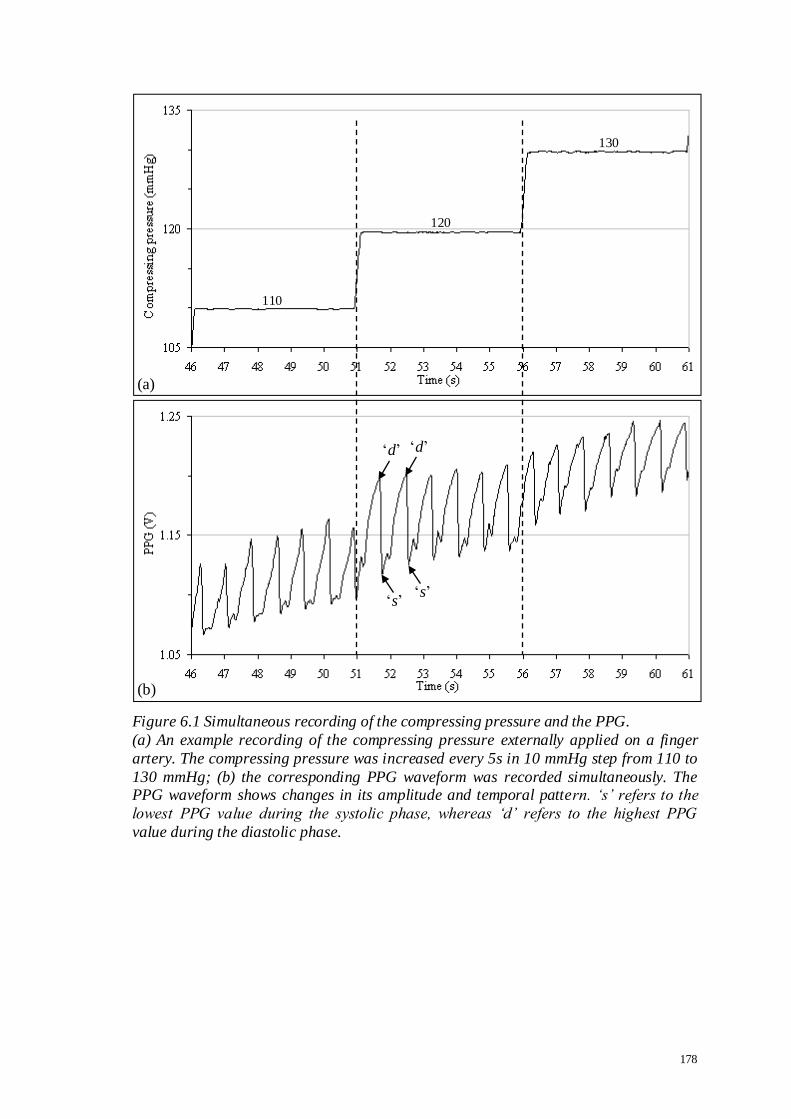
178
Figure 6.1 Simultaneous recording of the compressing pressure and the PPG.
(a) An example recording of the compressing pressure externally applied on a finger
artery. The compressing pressure was increased every 5s in 10 mmHg step from 110 to
130 mmHg; (b) the corresponding PPG waveform was recorded simultaneously. The PPG waveform shows changes in its amplitude and temporal pattern. „s‟ refers to the
lowest PPG value during the systolic phase, whereas „d‟ refers to the highest PPG
value during the diastolic phase.
110
120
130
(a)
(b)
‘d’
‘s’
‘d’
‘s’

179
Table 6.1 Relationship between pulsation amplitude and intra-arterial MAP.
This relationship was evaluated by authors in the articles listed below. A tick (✔) means
that a theoretical model was evaluated in the article. The last row refers to the
experimental setup in this chapter.
# Article Measurement
technique
Theoretical
model Experiment Subjects Artery
1. (Posey et al.,
1969) Oscillometric In vitro Dog Carotid
2. (Ramsey III,
1979) Oscillometric In vivo Human
Bicep /
calf / ankle
3. (Yelderman and
Ream, 1979) Oscillometric In vivo Human Brachial
4. (Mauck et al.,
1980) Oscillometric ✔ In vitro Dog Carotid
5. (Yamakoshi et
al., 1982)
Photo-
plethysmography In vitro Dog Carotid
6. (Forster and
Turney, 1986) Oscillometric ✔ Brachial
7. (Penaz, 1992) Volume
clamping
Not applicable
(review article) Human Finger
8. (Drzewiecki et
al., 1994) Oscillometric ✔ Brachial
9. (Wesseling et
al., 1995)
Volume
clamping
In vitro
In vivo
Human / rat
Human
Finger/tail
Finger
10. (Ursino and
Cristalli, 1996) Oscillometric ✔ Brachial
11. (Baker et al.,
1997) Oscillometric ✔ In vivo Dog Radial
12. (Raamat et al.,
1999) Oscillometric ✔ Finger
13. This chapter Volume
clamping In vivo Human Finger
180
The table shows that a large majority of the articles are based on the oscillometric
technique. Similar articles based on the volume clamping technique are very limited.
Studies that used the oscillometric technique cannot be directly compared with those
that used the volume clamping technique. This is due to differences in the working
principles of the measurement techniques, the measurement sites and the setup of the
studies. Furthermore, the pulse wave in oscillometry is due to the pressure oscillation in
the compressing chamber, e.g. the inflatable arm cuff. The pressure oscillation is
generated as the ABP is transmitted through the tissue to the cuff. In the volume
clamping technique, however, the pulse wave is due to the amount of illuminated light
being scattered or reflected by the pulsating blood volume in the artery to the
photodetector, which is then measured as the PPG.
The objectives of this chapter are:
i. To assess the relationship between the PPG peak pulsation amplitude and the MAP;
ii. To propose future modifications to the self-calibration algorithm in STAbp to
improve the Setpt determination.

181
6.2 Method
6.2.1 Subjects and Measurements
In this study, 5 subjects were recruited (3 males, 2 females, age (mean ± SD) 32 ± 15
years). The participants were all staff from the Medical Physics department. Consent
was given by each participant prior to the arrangement for the ABP measurements. The
study was approved by the Leicestershire ethics committee (reference number: 4680).
Two Finapres finger cuffs of appropriate size were fitted on the ipsilateral middle and
annulus fingers of the right hand. The fitting and positioning of the finger cuffs adhered
to the manufacturer’s guidelines. The finger cuff on the annulus finger was used to
measure the ABP with the Finapres. The finger cuff on the middle finger was operated
by an in-house built PPG recording device, which is a simpler version of the STAbp
system architecture described in Chapter 3. Referring to the block diagram in Figure
3.1, G9 sends out a required sequence of compressing pressures as command output
(R1). The mode switch (G11) connects R1 to G3 which supplies regulated compressing
pressure. G3 regulates the pressure in the finger cuff to compress the artery.
Simultaneously, G1 monitors the arterial blood volume change in the finger. Its output
is converted as PPG (G2) and sent (C1) to G9 to be recorded by the desktop computer.
A separate channel was used to record the ABP measured by the Finapres. Both the
Finapres and the PPG waveforms were simultaneously sampled at 100Hz (DT302, Data
Translation®). The recording was managed with the Agilent VEEPro® visual
programming software.
182
Two ipsilateral instead of contralateral fingers were used in order to minimise the
potential difference in regional regulation of arterial blood flow between the two hands.
The subjects had no known history of cardiovascular or other pathologies that would
affect the blood circulation in the fingers.
6.2.2 Protocols
Each subject attended two measurement sessions (Test #1 and Test #2). Throughout the
experiment, the right hand rested on a bench at heart level. The subjects were asked to
relax their fingers and breathe normally while sitting on a chair with back support. The
subjects were also asked not to engage in any conversation, laughter, holding their
breath or shifting about in their seated position. This is necessary to minimise artifacts
and to obtain stable physiological recordings.
In Test #1, the compressing pressure in the cuff (denoted as Pcom) was first increased by
approximately 10 mmHg every 5s. The range of Pcom encompassed the physiological
range of systolic and diastolic pressures. When Pcom had increased above systolic
pressure, the recording was complete. It was then decreased at the same rate until it was
near zero mmHg. This corresponded to a separate recording. The cycle of increasing
and decreasing the Pcom was then repeated, hence giving a total of four sets of
recordings.
In Test #2, the same setup and protocol were repeated except that the Pcom steps were
now changed at approximately 2 mmHg every 5s. Again, 4 sets of recordings were
obtained in each subject.
183
The Finapres has a built-in physiological self-calibration facility known as the
Physiocal (Wesseling et al., 1995). It was kept switched on throughout the ABP
measurement. This is to prevent any potential drifts in the MAP measured with the
Finapres.
6.2.3 Data Analysis
As was shown in Figure 6.1, the PPG pulse amplitude is measured between each ‘s’ and
the preceding ‘d’. It is denoted as PPGa (V). Depending on the pulse rate, 3 to 5 pulses
were recorded at each Pcom. The PPGa from these pulses during the same Pcom were
then averaged ( aPPG (SD)). Corresponding ABP pulses were recorded with the
Finapres, and the average (SD) of systolic, mean and diastolic pressures were also
computed (i.e. FSBP , FMAP and FDBP respectively). The array of aPPG was
plotted against the sequence of Pcom. Figure 6.2(a) shows an example.
Next, the pressure difference (Pdiff) was defined as
Pdiff = FMAP - Pcom (6.1)
Pdiff was calculated for each Pcom. The aPPG array was then replotted against the Pdiff
(Figure 6.2(b)). The aPPG array was fitted with a polynomial curve (
PPGa) for the
pressure range of ±40 mmHg around Pdiff = 0. The first to sixth order polynomials were
tested to compare the RMSE of different fitted curves on the aPPG array.

184
Referring to Figure 6.2(b) again, the
PPGa curve usually shows a peak. The
corresponding Pdiff to this peak was retrieved. This is denoted as PdiffA (mmHg). At Pdiff
= 0, Equation 6.1 shows that Pcom equals to FMAP . Hence, PdiffA indicates the difference
between the Pcom at the peak of the
PPGa curve and the Pcom at Pdiff = 0. Figure 6.2(b)
shows an example where a positive PdiffA is obtained, whereas Figure 6.2(c) shows an
example where a negative PdiffA is obtained.
Statistical Analysis
Provided that all measurements were satisfactory, eight PdiffA values would be available
per subject. The Kolmogorov-Smirnov normality test was first carried out from all
available PdiffA. If the distribution was normal, subsequent data analysis would use
parametric statistical methods. The collection of PdiffA was then tested to assess if it is
significantly different from zero mmHg.
Two hypotheses were defined. The first null hypothesis states that PdiffA is not different
from zero. If this is true, statistical analysis is completed. However, if the hypothesis is
rejected, the second null hypothesis states that the setup and protocols in Tests #1 and
#2 do not lead to significant differences in PdiffA.
According to the setup and protocols in Tests #1 and #2, three factors were identified
applicable to each subject. Each factor was tested for non-significant differences in
PdiffA. For the first factor, it refers to repeated measurements. Second, the direction of
the Pcom sequence was reversed. Third, the step interval of Pcom was changed. Multiple
comparisons were required and for this reason a hierarchical testing approach was
adopted. If the parametric methods were appropriate, paired two-tail t-test would be

185
used for the multiple comparisons. Otherwise, the Wilcoxon non-parametric test would
be applied.
The hierarchical test began with the repeated measurements factor. Measurement results
with the 2 mmHg step interval were first tested (i.e. higher resolution). This was
followed by the direction of the Pcom sequence. Lastly, the influence of the step interval
of Pcom was tested. If the statistical result in each level showed no significant difference,
the corresponding PdiffA values were pooled by averaging per subject before the next
level of the hierarchy was tested. A value of p <0.05 was taken as the level of statistical
significance. Bonferroni correction was applied to account for multiple comparisons
(Bland, 1995; Campbell and Machin, 1995), with the α-levels corrected to 0.05, 0.025
and 0.017 for the three factors respectively.

186
Figure 6.2 Example computation of PdiffA from the GaPP ˆ curve.
(a) Example of aPPG array plotted against the sequence of decreasing Pcom.; (b)
the aPPG array was replotted against Pdiff. It is superimposed with a polynomial fitted
curve (denoted as
PPGa). The error bars are ±1SD. The PdiffA is indicated. In this example, a positive PdiffA is obtained; (c) another example where a negative PdiffA is
obtained.
(a)
(b)
(c)
PdiffA
PdiffA
PPGa
PPGa

187
6.3 Results
Good quality PPG recordings with stable Finapres ABP waveforms were obtained in all
measurements. In each of the Tests #1 and #2, four sets of recordings were obtained,
hence there were eight sets per subject. As there were five subjects, a total of 40 PdiffA
values would be available.
Figure 6.3 shows the RMSE (mean ± SD) for each of the first to sixth order polynomials
fitted to every aPPG array. Two graphs were plotted to show the respective mean
RMSE for Tests #1 and #2. Each mean RMSE was computed from 20 individual
RMSE. Both plots show that above the fourth order, the RMSE does not decrease
significantly with higher order polynomials. Therefore, for further data analysis, each of
the aPPG arrays was fitted with the fourth order polynomial curve. It is to note that the
fitted curve was denoted as
PPGa to differentiate it from the aPPG array.
Figure 6.4 shows an example of the data analysis process to obtain PdiffA. Figure 6.4(a)
shows that the Finapres FSBP , FMAP and FDBP were stable as Pcom was decreased at
2 mmHg steps every 5s. Figure 6.4(b) shows the array of aPPG with decreasing Pcom.
The Pdiff was computed (Equation 6.1) for the horizontal axis and the figure was
replotted in Figure 6.4(c). The aPPG array is shown superimposed by the
PPGa fitted
curve. PdiffA was identified from the
PPGa curve. In this example, PdiffA = 6.2 mmHg.
The process above was repeated for all other aPPG arrays to obtain their respective
PdiffA.

188
Figure 6.3 RMSE of the polynomial curve fitting of aPPG arrays. Each mean RMSE was computed from 20 individual RMSE. First to sixth order
polynomials were fitted on each of the aPPG arrays for Test #1 (square) and Test #2 (cross). The graphs are slightly shifted from each other to avoid superposition of the
error bars. The error bars are the respective ±1SD. The fourth order (indicated by an
arrow) has been chosen for the data analysis in this study.

189
Figure 6.4 Computation of PdiffA from the GaPP ˆ curve.
(a) The Pcom (light square) was decreased at 2 mmHg steps every 5s. The Finapres ABP
is shown as: FSBP (diamond), FMAP (square) and FDBP (triangle); (b) the array of
aPPG corresponding to decreasing Pcom; (c) graph in (b) was replotted against Pdiff
(Equation 6.1). The aPPG array is superimposed by the fourth order polynomial curve
(
PPGa). The PdiffA is indicated. In this example, PdiffA = 6.2 mmHg. In all the graphs, the error bars are the respective ±1SD.
(a)
(b)
(c)
PdiffA
PPGa

190
Table 6.2 presents all the 40 individual results of PdiffA from the five subjects. Figure 6.5
shows the histogram of the sample distribution. Seven out of the 40 PdiffA (17.5%) are
positive values, while the remaining 82.5% are negative values. The positive PdiffA are
also shown in bold in the table. The Kolmogorov-Smirnov test showed that the
distribution was normal (p>0.20). PdiffA was significantly different from zero mmHg
(paired t-test, p<0.001). Hence, the first null hypothesis was rejected.
For the second hypothesis, the hierarchical statistical tests for PdiffA showed no statistical
significance for the three factors. It is to note that when no statistical significance was
detected from the paired t-test at each level of the hierarchy, the PdiffA values were
pooled to obtain an average value. Hence, the mean (SD) of differences between PdiffA in
the repeated measurements factor (p>0.20, n = 5 subjects) were:
2.0 (3.91) mmHg for increasing Pcom sequence at 2 mmHg step interval;
0.8 (1.16) mmHg for decreasing Pcom sequence at 2 mmHg step interval;
1.8 (5.70) mmHg for increasing Pcom sequence at 10 mmHg step interval;
2.1 (5.84) mmHg for decreasing Pcom sequence at 10 mmHg step interval.
Next, the mean (SD) of differences between PdiffA for the factor on direction of Pcom
sequence (p>0.20, n = 5 subjects) were:
0.3 (2.38) mmHg at 2 mmHg step interval in Pcom;
2.3 (3.61) mmHg at 10 mmHg step interval in Pcom.
Finally, the mean (SD) of differences between PdiffA for the factor on step interval of
Pcom was computed as -0.4 (4.27) mmHg. With the second null hypothesis accepted, this

191
means that the setup and protocols in Tests #1 and #2 did not lead to significant
differences in PdiffA.
The PdiffA in Table 6.2 are plotted in Figure 6.6(a) according to subjects. With the
exception of subjects 1 and 3, all other subjects only have distributions with PdiffA < 0.
The intra-subject mean (SD) of PdiffA are shown in Figure 6.6(b). It is replotted with
respect to the subjects’ age (Figure 6.6(c)). No significant correlation with age was
detected.
In summary, with the PdiffA results giving a normal distribution and no statistical
significance detected for the three factors considered, the sample average (mean (SD))
for PdiffA was computed as -4.7 (5.63) mmHg.
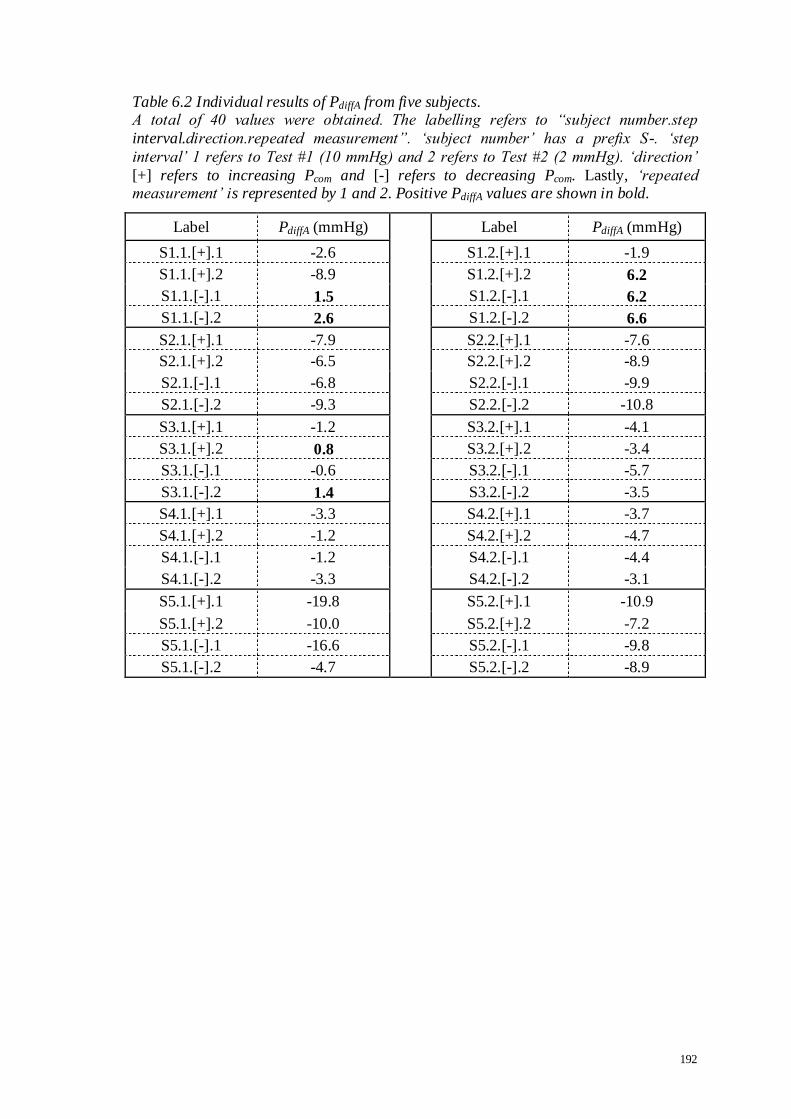
192
Table 6.2 Individual results of PdiffA from five subjects. A total of 40 values were obtained. The labelling refers to “subject number.step
interval.direction.repeated measurement”. „subject number‟ has a prefix S-. „step
interval‟ 1 refers to Test #1 (10 mmHg) and 2 refers to Test #2 (2 mmHg). „direction‟
[+] refers to increasing Pcom and [-] refers to decreasing Pcom. Lastly, „repeated measurement‟ is represented by 1 and 2. Positive PdiffA values are shown in bold.
Label PdiffA (mmHg) Label PdiffA (mmHg)
S1.1.[+].1 -2.6 S1.2.[+].1 -1.9
S1.1.[+].2 -8.9 S1.2.[+].2 6.2
S1.1.[-].1 1.5 S1.2.[-].1 6.2
S1.1.[-].2 2.6 S1.2.[-].2 6.6
S2.1.[+].1 -7.9 S2.2.[+].1 -7.6
S2.1.[+].2 -6.5 S2.2.[+].2 -8.9
S2.1.[-].1 -6.8 S2.2.[-].1 -9.9
S2.1.[-].2 -9.3 S2.2.[-].2 -10.8
S3.1.[+].1 -1.2 S3.2.[+].1 -4.1
S3.1.[+].2 0.8 S3.2.[+].2 -3.4
S3.1.[-].1 -0.6 S3.2.[-].1 -5.7
S3.1.[-].2 1.4 S3.2.[-].2 -3.5
S4.1.[+].1 -3.3 S4.2.[+].1 -3.7
S4.1.[+].2 -1.2 S4.2.[+].2 -4.7
S4.1.[-].1 -1.2 S4.2.[-].1 -4.4
S4.1.[-].2 -3.3 S4.2.[-].2 -3.1
S5.1.[+].1 -19.8 S5.2.[+].1 -10.9
S5.1.[+].2 -10.0 S5.2.[+].2 -7.2
S5.1.[-].1 -16.6 S5.2.[-].1 -9.8
S5.1.[-].2 -4.7 S5.2.[-].2 -8.9

193
Figure 6.5 Histogram for the sample distribution of PdiffA.
Table 6.2 shows the individual results of PdiffA. The Kolmogorov-Smirnov test showed that the sample distribution was normal.
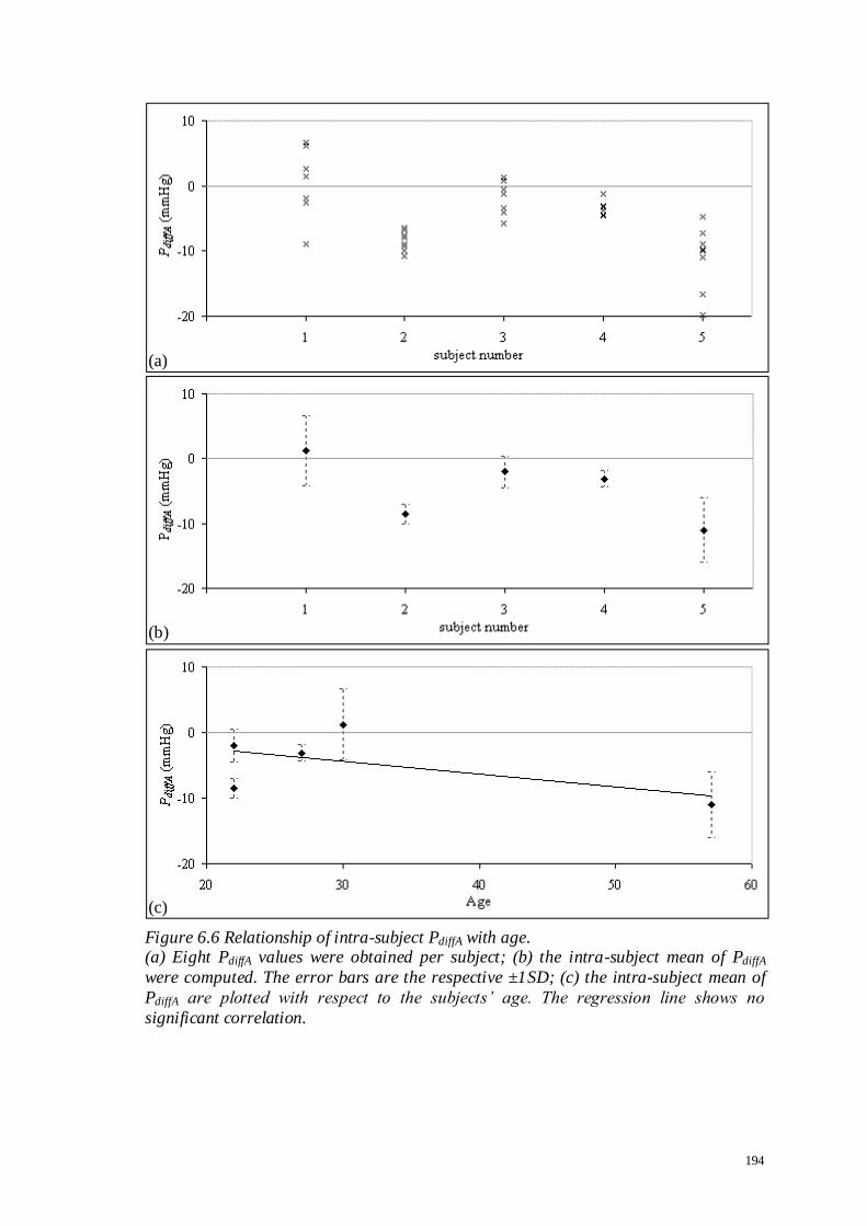
194
Figure 6.6 Relationship of intra-subject PdiffA with age. (a) Eight PdiffA values were obtained per subject; (b) the intra-subject mean of PdiffA
were computed. The error bars are the respective ±1SD; (c) the intra-subject mean of
PdiffA are plotted with respect to the subjects‟ age. The regression line shows no
significant correlation.
(a)
(b)
(c)

195
6.4 Discussion
The level of detail presented in this chapter exceeds those of the published literature.
This is particularly the case of the volume clamping technique. The advantage of the
study in this chapter is that in vivo setup was used on human artery (see Table 6.1).
Noteworthy, the study dealt with physiological measurements in humans. This
resembles the actual setup of continuous ABP monitoring. Thus, the results are more
representative to the STAbp prototype device described in chapter 3 and evaluated in
chapter 4.
6.4.1 Main Findings
The statistical outcome of the first null hypothesis with the PdiffA significantly different
from zero mmHg indicates that the peak of
PPGa curve does not coincide with the
MAP estimated with the Finapres. Furthermore, the normally distributed PdiffA (Figure
6.5) means that a simple correction of addition or subtraction of a constant value may
not be suitable. Such phenomenon may affect the accuracy and reliability of ABP
measurements in some individuals. On the other hand, it was demonstrated that PdiffA
was not influenced by the three factors, i.e. repeated measurements, direction of the Pcom
sequence and the step interval of Pcom.
6.4.2 Previous Work
From the list of articles in Table 6.1, Ramsey III (1979) and Yamakoshi et al. (1982)
reported that at the largest pulsation amplitude in oscillometry, the cuff pressure

196
coincided with the intra-arterial MAP. Penaz (1992) concluded the same except that it
was based on the volume clamping technique. Conversely, a much larger number of
articles (Table 6.1 numbered 1, 3, 4, 6, and 8-12) reported that the largest pulsation
amplitude did not coincide with the MAP. The difference between the cuff pressure at
this largest pulsation amplitude and the MAP was found to be small. The reported mean
(SD) of differences were -0.2 (4.21) mmHg (Ramsey III, 1979), 1.4 (6.22) mmHg
(Yelderman and Ream, 1979), within ±3 mmHg (Yamakoshi et al., 1982), within 2
mmHg (Drzewiecki et al., 1994), and ranged from -8 to 19 mmHg (Raamat et al., 1999).
It is to note that the setup and protocols of these results are different from the study
presented in this chapter. Most of these articles were based on the oscillometric
technique (Table 6.1 numbered 1-4, 6, 8 and 10-12). In addition to the different
measurement techniques used, the studies included the use of excised animal arteries
(numbered 1, 4, 5, 9 and 11), in vitro setup (numbered 1, 4, 5 and 9), theoretical
modelling (numbered 4, 6, 8 and 10-12) and subjects with a wide range of existing
pathologies (numbered 2, 3 and 9). The diversity of techniques, subjects and
preparations do not allow direct comparison with the results of this chapter.
6.4.3 Implications from Findings
A possible solution for implementation into the STAbp device is to reduce the Pcom by
4.7 mmHg in order to improve agreement with the MAP (Equation 6.1). At this
compressing pressure (i.e. (Pcom - 4.7) mmHg), the corresponding PPG pulse is
retrieved. The mean of this PPG pulse may then be used as the Setpt in the STAbp. To
implement this in the STAbp, it is not a simple numerical calculation but requires a more
extensive review of the existing software algorithm.
197
6.4.4 Limitations of the Study
Several limitations were identified in this experiment:
i. The evaluation of the experiment was based on a small sample size. Statistical
power analysis was not carried out a priori to determine a suitable sample size as
relevant sample SD was not available in existing literature. For the benefits of
future studies, the power analysis was calculated retrospectively. To detect a
difference of 5 mmHg (O'Brien and Atkins, 1994) for PdiffA using the estimated
value of SD = 5.63 mmHg, with 80% power at 0.05 level of significance for paired
data (Campbell and Machin, 1995), ten subjects would be required;
ii. The MAP in Equation 6.1 was computed from the Finapres ABP waveforms. As
demonstrated in the comparative study between two Finapreses (section 4.3), there
are inherent differences even with monitoring devices of the same specification and
model number. The accuracy of the Finapres ABP measurement may need to be
interpreted with caution. Nevertheless, this was the best means for comparisons at
the time of the experiment;
iii. The experiment was carried out on the finger arteries instead of the STA. Due to
their different locations, it remains to be determined if the results obtained in this
study are transferable to the STA;
iv. The experiment was carried out on healthy adults. It is uncertain if the results can
be used in teenagers and those younger or the very old, and in subjects with specific
conditions (e.g. atherosclerosis, hypertension, diabetes, obesity and others);
v. The recordings were based on resting condition, it is uncertain if the same results
would be obtained in situations with varying ABP such as exercise or specific
manoeuvres such as Valsalva;

198
vi. The measurement protocols in Tests #1 and #2 are not practical to search for the
appropriate Setpt during real time ABP measurement. A large number of PPG
pulses is required to construct the aPPG array. During the recording of the PPG
waveform, the continuous ABP waveform becomes unavailable;
vii. The polynomial curve fitting was applied on the pressure range of ±40 mmHg
around Pdiff = 0. A change in this pressure range may affect the result of the PdiffA;
viii. Only the PPG pulse amplitude has been evaluated in this chapter. Other
characteristics of the PPG waveform have not been assessed (Figure 6.1), for
instance, the temporal pattern and the frequency content of the PPG waveform.
6.4.5 Suggestions for Future Work
The relationship between the PPG peak pulsation amplitude and the MAP may be more
complex than previously anticipated. Additional parameter(s) may be required to
develop a more robust algorithm for Setpt determination. One possible future work is to
further evaluate the temporal pattern and the frequency content of the PPG waveform.
To increase the confidence of the PdiffA results, another suggestion is that the experiment
described in this chapter may need to be repeated on the STA and evaluated with
intravascular measurements. Future studies will also require a larger number of subjects,
including different ages and clinical conditions.

199
6.5 Conclusion
The study presented in this chapter demonstrated that the peak of the PPG pulsation
amplitude does not coincide with the MAP estimated with the Finapres device. The
PdiffA is not a constant value which could be applied as a general correction factor since
it shows both intra- and inter-subject variability. Instead, the differences are normally
distributed. Further evaluation of the PPG waveform is suggested as this may help to
provide more answers to improve the determination of Setpt in the STAbp.

200
CHAPTER 7 CONCLUSIONS
7.1 Review of Objectives
This thesis focuses on ABP monitoring that generates continuous ABP waveforms. The
applications of continuous ABP waveforms encompass a wide range of clinical
assessments and physiological research (section 1.3). To encourage wider use of
continuous ABP monitoring, the noninvasive approach is preferred. The main benefits
of CoNIBP monitoring include better patient safety (i.e. minimise infection and other
clinical complications) and minimal running costs.
Currently available ABP measurement devices have several limitations that form the
rationale of this thesis (section 1.2). Section 1.2 also explained the reservations of
accepting ABP waveforms measured in the periphery to represent the ABP waveform
close to the heart (i.e. ascending aorta). These are due to the effects of pulse wave
propagation and reflection, differences in local regulations of blood flow, vasomotor
tone, arterial elasticity, peripheral resistance, and poor accuracy and reliability to
measure peripheral ABP in some patients groups.
The STA is evaluated as the best available alternative measurement site closer to the
heart for CoNIBP measurement (section 2.3). The effect of pulse wave propagation and
reflection is less prominent than peripheral ABP derived at the finger artery. For this
reason, it should be able to predict ABP in the ascending aorta more accurately.

201
A new CoNIBP measurement device, known as the STAbp, was designed and
constructed (chapter 3) and then evaluated (chapter 4). Further investigations were
carried out (chapters 5 and 6) to seek new knowledge and to consider a more robust
algorithm to improve the accuracy of ABP measurement with the STAbp. These further
investigations focused on the appropriate Setpt determination, first by assessing the
sensitivity of the ABP to perturbation of the Setpt, and then followed by further
assessment of PPG waveform to extract information which could be incorporated into
the STAbp to improve the Setpt determination, hence more accurate ABP waveform
recordings.
To a large extent these original objectives have been met with the design, construction
and testing of the new CoNIBP device. The main conclusions of this work are reviewed
in the following sections.

202
7.2 Original Contributions of Thesis
STAbp system architecture
The design and construction of the STAbp prototype device (chapter 3) allowed
continuous recording of ABP in the STA. The STAbp was developed based on the
volume clamping technique with photoplethysmography. It consists of a complex
integration of hardware and software components in order to monitor the ABP in the
STA with intermittent review of the PPG Setpt to ensure an accurate ABP waveform is
obtained. The intermittent review of the Setpt is carried out by the self-calibration
feature in the STAbp.
Evaluation of STAbp device
The STAbp provided physiologically realistic ABP waveforms with consistent baseline
stability (chapter 4). The widespread use of the STAbp device in the experiments
described in this thesis confirmed its relative reliability and robustness to routine use
despite only being a prototype constructed in-house. It was used in the experiments
described in chapters 3 to 5 with at least 35 ABP measurement sessions of five to fifteen
minutes each. The continuous ABP tracing also responded to manoeuvres such as the
Valsalva and the IHG exercise in similar fashion to what has been reported with
invasive ABP measurements.
An original assessment of the comparative performance of two Finapreses was
conducted to provide the background against which to compare the STAbp with the
Finapres. The comparisons between two Finapreses produced results which describe
their inherent differences even though both devices have the same specifications and

203
same model number. The differences in measurements could be caused by inappropriate
fitting of the finger cuff on the finger, motion artifacts or other physiological conditions
that may vary between both fingers. Technical differences in both devices are also
potential causes of error.
The spectral analyses between simultaneous ABP measurements by the two Finapreses
produced a relatively low cut-off frequency in the gain spectral curve (13.3 Hz) with
coherence above 0.5 only up to approximately 12.5 Hz (Figure 4.18). Nevertheless, the
comparative study between two Finapreses formed the necessary boundaries for
interpreting the results in the comparative study of the STAbp and Finapres more
appropriately.
In the comparative study of STAbp and Finapres, significant differences were obtained
in the agreement of the SBP, MAP, and DBP, as well as the ABP pulse bandwidth
limits. However, the assessment of ABP drift did not show significant differences which
suggest that the STAbp is at least as stable as the Finapres when the ABP in the STA is
monitored continuously. Given the fact that the differences of ABP waveshapes and
amplitude in different measurement sites, the spectral analyses gave a cut-off frequency
in the gain spectral curve lower than 13.3 Hz with a more complex phase response that
increases in phase leading between 3.2 Hz and 9.5 Hz up to approximately 110º before
stabilising (Figure 4.18). The magnitude squared coherence was retained above 0.5 even
beyond 12.5 Hz which is approximately as good as the coherence spectrum between
two Finapreses.

204
Further investigations
Following chapter 4, further research studies (chapters 5 and 6) first reported the high
sensitivity of the ABP waveform to a small change in Setpt, which indicates the need
for more stringent selection of hardware components to ensure that the Setpt will not be
affected by technical issues such as electronic drift, noise and thermal interferences.
Greater attention must also be given in future reviews to the software algorithm that
determines the Setpt. Additionally, the studies also reported that the PPG waveform
contains additional information that may contribute to the improvement of the self-
calibration algorithm for Setpt determination. One aspect of the PPG waveform
analysed was the difference between the external compressing pressure at the PPG peak
pulsation amplitude and the MAP. The sample average of the differences was
considered small (-4.7 mmHg), however, the differences were not constant intra- and
inter- subjects, but tended to follow a normal distribution.
The availability of the STAbp offers many advantages to the research and clinical
communities. The monitoring of the ABP in the STA could be a useful tool to study the
pathophysiology of human vascular circulation in the head intra- and extra- cranially. It
is also a step forward towards comparing the blood flow and the ABP in the STA
simultaneously. These will potentially extend the scope of human physiological
research which was not explored previously.

205
7.3 Limitations of the Thesis
The evaluation of the STAbp was compared to the Finapres. Finapres is currently the
best alternative to the gold standard, i.e. intravascular measurement. Inherent
differences learnt in the comparative study between two Finapreses (section 4.3)
indicate the importance of this prior knowledge before the measurement differences
between the STAbp and Finapres (section 4.4) could be evaluated. However, with the
influence of pulse wave propagation and reflection, local blood flow regulation,
vasomotor tone, arterial elasticity and peripheral resistance, the comparisons of the ABP
between these different measurement sites are not definitive.
The subjects recruited for the studies described in the thesis are all relatively young
healthy adults with no known pathologies that may affect their blood circulation. The
validity of the analysis results obtained may not be applicable to teenagers and those
younger or the elderly, and to individuals with specific conditions such as hypertension,
cardiac dysfunction, obesity, atherosclerosis or diabetes.

206
7.4 Suggestions for Future Work
The design of the head frame needs to be modified to improve its stability and fitting
during continuous ABP monitoring. It is also necessary to provide enough flexibility for
optimal adjustment with varying human head sizes. With current head frame design, the
subjects were required to sit in an upright position. A new design is needed to allow
subjects to lie in a supine position. Such design will also be more suitable clinically for
patients who are not able to sit up for a prolonged duration.
The effect of different surface areas of compression from the front of the probe on the
skin with underlying STA needs to be investigated further. This could be carried out in
conjunction with exploring the different arrangements of optoelectronic components
relative to the STA. The accuracy and reliability of the PPG waveform produced will
need further investigation to identify factors that can interfere with the intended PPG
output. At the same time, the PPG waveshape can be analysed further to produce new
information that may be incorporated into the self-calibration algorithm in the STAbp to
improve the robustness of Setpt determination.
The use of mathematical modelling or a specific experimental test rig could be
beneficial to evaluate these variables. It is envisaged that the benefits of mathematical
modelling could be multi-fold. These include a better understanding of the mechanical
properties of STAbp design, for instance, the area of compression of the probe on the
tissue with the underlying STA; a better understanding of the optical properties of the
artery, the surrounding tissue and the bone at the temporal region; a better
understanding of factors that can affect the PPG waveshape; and to predict the accuracy

207
of ABP waveform measured with the STAbp on patient, age and fitness level specific
groups.
For validation of the prototype device, an important step forward will be to validate the
STAbp against intravascular measurement i.e. ABP in the ascending aorta. This is
merited by the encouraging results obtained so far, however it must only be considered
after further improvements as suggested above.
Successful validation in comparison with an intravascular catheter-tip transducer in the
ascending aorta must be followed by wider evaluation to include different age groups
and patients with different conditions, particularly those with increased arterial stiffness
or other pathologies that might affect the difference between peripheral and central
measures of ABP.

208
7.5 Conclusions
The evaluation of the STAbp prototype device demonstrated the ability of the device to
produce realistic ABP waveforms and its comparison with Finapres showed reasonable
agreement. Nevertheless, further hardware developments and software improvements
are still necessary before its validation against central intravascular measurement.
Further validation in different age groups and patients is also a future target.
The availability of the STAbp will provide easier access to a CoNIBP measurement
device beneficial for clinical assessments and physiological research. Wider utilisation
of CoNIBP measurements is likely to lead to considerable additional knowledge that
will further improve the prognosis, diagnosis and management of patients with
cardiovascular disease and other conditions.

209
APPENDIX ELECTRONIC CIRCUITS DIAGRAMS
Figure A.1 IRED Driver and Transimpedance Amplifiers
NB: This is G1 in Figure 3.1.
NB: This is G1 in Figure 3.1.
IRED Driver Circuit
A
C
70 Ohm
+5V
Built inside probe
(see section 3.3.1)
Transimpedance Amplifiers
-
+
390k
OPA4132
-
+
390k
OPA4132
-
+
390k
OPA4132
-
+
390k
OPA4132
PD4
PD3
PD1
PD2
MAX4534CUD
PD4
PD3
PD1
PD2
Output for
PPG signal
generation (G2)
A
C
A
C
A
C
A
C
Built inside probe
(see section 3.3.1)
SME2470
SMD2420
Multiplexer
Legend:
PD = photodetector

210
Figure A.2 Piezo Valve with Regulated Compressed Air Supply
-15V
Exhaust / relief port
Inlet Outlet to
sealed air chamber
G7
Regulated Compressed Air Supply
Hoerbiger-Origa PS11010-31LR
Medo
AC0105
Air
Compressor PrTx 2
Pressure
transducer 2
Airtrol
F-4200-15
Pressure switch
(see section 3.3.3)
±V
Electrical
Mains Supply
NB: This is G4 in Figure 3.4.
NB: This is G6
in Figure 3.4 Piezo Valve
Control Input,
from G5
Airtrol
R-920-10
Pressure
regulator

211
Figure A.3 Controller (for Regulated Compressing Pressure)
R1 or C3 Required
Compressing
Pressure
NB: This is G5 in Figure 3.4.
-
+ INA105KU
Differential
Amplifier
Real-time transducer
pressure
100kvar
LM324
2k -
+
Proportional
error
-
+
200kvar
1n
LM324
500kvar
LM324
1k -
+
Derivative
Integrator
10n
1n
2k
2k
2k
-
+
LM324
Summing
Amplifier
Output to piezo valve
G6
C2
2k

212
Figure A.4 Pressure Transducer
Output
-
+
Instrumentation Amplifier
AD620R 26PC05SMT
Pressure sensor 360 Ohm
Offset
Adjust
+5V
+
- OP113FS
Offset Adjust
5kvar
3.6k
-5V
+5V
NB: This is G8 in Figure 3.4.
C2

213
Figure A.5 PPG Signal Generation
NB: This is G2 in Figure 3.1.
-
+ 82k 4.7k
0.1u
0.47u
TL074
-
+ 68k 5.6k
0.1u
0.47u
TL074
-
+ 56k 6.8k
0.1u
0.47u
TL074
-
+ 18k 10k
0.1u
0.68u
TL074
-
+ Input INA105
49.5k
TL074 Output
1k
-
+
(from G1)
Non-inverting Gain Amplifier
Differential Amplifier
C1
8th order unity gain Bessel
Sallen-Key 20Hz low-pass filter
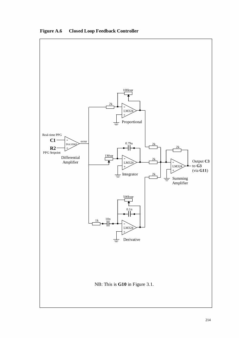
214
Figure A.6 Closed Loop Feedback Controller
NB: This is G10 in Figure 3.1.
-
+
PPG Setpoint
INA105KP
Differential
Amplifier
Real-time PPG
100kvar
LM324
2k -
+
Proportional
error
-
+
1Mvar
0.79u
LM324
500kvar
LM324
1k -
+
Integrator
10n
0.1n
2k
2k
2k
-
+
LM324
Summing
Amplifier
Output C3
to G3
(via G11)
Derivative
C1
R2 2k

215
Figure A.7 Mode Switch
NB: This is G11 in Figure 3.1.
HEF4027
Dual JK
flip-flop
Activate OLP
Activate CLP
Legend:
OLP = Open Loop Procedure (see description in section 3.3.7.1) CLP = Closed Loop Procedure (see description in section 3.3.7.2)
(R1 or C3)
to G3
Analog switch
DG211BDJ
C3
R1
Digital input
(VeePro® controlled)
-
+
R1 Required
compressing
pressure LM311N
Voltage
Comparator
C3
controller
output from
G10
OLP:
CLP:

216
BIBLIOGRAPHY
Aaslid, R., Lindegaard, K.F., Sorteberg, W. and Nornes, H., 1989. Cerebral autoregulation dynamics in humans. Stroke, 20(1), 45-52.
Allen, J., 2007. Photoplethysmography and its application in clinical physiological measurement. Physiol Meas, 28(3), R1-R39.
Amoore, J.N., Guehenec, M., Scordecchia, R. and Scott, D.H., 2010. Auditing the technology used to measure blood pressure. J Med Eng Technol, 34(3), 209-216.
Andriessen, P., Schoffelen, R.L., Berendsen, R.C., de Beer, N.A., Oei, S.G., Wijn, P.F. and Blanco, C.E., 2004. Noninvasive assessment of blood pressure variability in
preterm infants. Pediatr Res, 55(2), 220-223.
Astrom, K.J. and Hagglund, T., 1995. PID controllers: theory, design and tuning. 2nd
edn, North Carolina: International Society of Automation.
Atkins, E.R., Brodie, F.G., Rafelt, S.E., Panerai, R.B. and Robinson, T.G., 2010.
Dynamic cerebral autoregulation is compromised acutely following mild ischaemic
stroke but not transient ischaemic attack. Cerebrovasc Dis, 29(3), 228-235.
Aubert, A.E., Vrolix, M., de Geest, H. and van de Werf, F., 1995. In vivo comparison
between two tip pressure transducer systems. Int J Clin Monit Comput, 12(2), 77-83.
Avolio, A., 1992. Ageing and wave reflection. J Hypertens Suppl, 10(6), S83-S86.
Avolio, A.P., Deng, F.Q., Li, W.Q., Luo, Y.F., Huang, Z.D., Xing, L.F. and O'Rourke,
M.F., 1985. Effects of aging on arterial distensibility in populations with high and low
prevalence of hypertension: comparison between urban and rural communities in China.
Circulation, 71(2), 202-210.
Baguley, I.J., Heriseanu, R.E., Cameron, I.D., Nott, M.T. and Slewa-Younan, S., 2008.
A critical review of the pathophysiology of dysautonomia following traumatic brain injury. Neurocrit Care, 8(2), 293-300.
Baker, P.D., Westenskow, D.R. and Kuck, K., 1997. Theoretical analysis of non-invasive oscillometric maximum amplitude algorithm for estimating mean blood
pressure. Med Biol Eng Comput, 35(3), 271-278.
Bedford, R.F., 1978. Long-term radial artery cannulation: effects on subsequent vessel
function. Crit Care Med, 6(1), 64-67.
Bedford, R.F. and Wollman, H., 1973. Complications of percutaneous radial-artery
cannulation: an objective prospective study in man. Anesthesiology, 38(3), 228-236.

217
Belardinelli, E. and Cavalcanti, S., 1992. Theoretical analysis of pressure pulse propagation in arterial vessels. J Biomech., 25(11), 1337-1349.
Bendat, J.S. and Piersol, A.G., 1986, Digital Data Analysis. Random Data: Analysis and Measurement Procedures, 2nd edn, New York: John Wiley & Sons, Chapter 11, 361-
424.
Bendat, J.S. and Piersol, A.G., 1993. Engineering Applications of Correlation and
Spectral Analysis. New York: Wiley.
Bergersen, T.K., 1993. A search for arteriovenous anastomoses in human skin using
ultrasound Doppler. Acta Physiol Scand, 147(2), 195-201.
Bienfang, D.C., 1984. Use of the Doppler probe to detect the course of the superficial
temporal artery. Am J Ophthalmol, 97(4), 526-527.
Birch, A.A., Dirnhuber, M.J., Hartley-Davies, R., Iannotti, F. and Neil-Dwyer, G.,
1995. Assessment of autoregulation by means of periodic changes in blood pressure.
Stroke, 26(5), 834-837.
Birch, A.A. and Morris, S.L., 2003. Do the Finapres and Colin radial artery tonometer
measure the same blood pressure changes following deflation of thigh cuffs? Physiol
Meas, 24(3), 653-660.
Bland, J.M. and Altman, D.G., 1986. Statistical methods for assessing agreement
between two methods of clinical measurement. Lancet, 1(8476), 307-310.
Bland, M., 1995, Significance tests. An introduction to medical statistics, 2nd edn, New
York: Oxford University Press, Chapter 9, 133-151.
Blank, S.G., West, J.E., Muller, F.B., Cody, R.J., Harshfield, G.A., Pecker, M.S.,
Laragh, J.H. and Pickering, T.G., 1988. Wideband external pulse recording during cuff deflation: a new technique for evaluation of the arterial pressure pulse and measurement
of blood pressure. Circulation, 77(6), 1297-1305.
Bloomfield, P., 2000. Fourier analysis of time series : an introduction. 2nd edn, New
York: Wiley.
Boehmer, R.D., 1987. Continuous, real-time, noninvasive monitor of blood pressure:
Penaz methodology applied to the finger. J Clin Monit, 3(4), 282-287.
Brigham, E.O., 1988. The fast Fourier transform and its applications. Englewood Cliffs,
NJ: Prentice-Hall International.

218
Brinton, T.J., Cotter, B., Kailasam, M.T., Brown, D.L., Chio, S.S., O'Connor, D.T. and DeMaria, A.N., 1997. Development and validation of a noninvasive method to
determine arterial pressure and vascular compliance. Am J Cardiol, 80(3), 323-330.
Brown, T.R. and MacGregor, J., 1982. An infra-red reflectance system for ambulatory
characterization of left ventricular function. J Biomed Eng, 4(2), 142-148.
Bull, M.J., Schreiner, R.L., Garg, B.P., Hutton, N.M., Lemons, J.A. and Gresham, E.L.,
1980. Neurologic complications following temporal artery catheterization. J Pediatr,
96(6), 1071-1073.
Burr-Brown, 1997. ISO 124 Isolation Amplifier. Burr-Brown, USA: Texas Instruments
Incorporated, 1-12.
Cameron, J.D., McGrath, B.P. and Dart, A.M., 1998. Use of radial artery applanation
tonometry and a generalized transfer function to determine aortic pressure augmentation
in subjects with treated hypertension. J Am Coll Cardiol, 32(5), 1214-1220.
Campbell, M.J. and Machin, D., 1995. Medical Statistics: a commonsense approach.
2nd edn, Chichester, West Sussex: John Wiley & Sons.
Carroll, G.C., 1988. Blood pressure monitoring. Crit Care Clin, 4(3), 411-434.
Celis, H. and Fagard, R.H., 2004. White-coat hypertension: a clinical review. Eur J
Intern Med, 15(6), 348-357.
Chemla, D., Antony, I., Zamani, K. and Nitenberg, A., 2005. Mean aortic pressure is the
geometric mean of systolic and diastolic aortic pressure in resting humans. J Appl
Physiol, 99(6), 2278-2284.
Chen, C.H., Ting, C.T., Lin, S.J., Hsu, T.L., Yin, F.C., Siu, C.O., Chou, P., Wang, S.P.
and Chang, M.S., 1995. Different effects of fosinopril and atenolol on wave reflections in hypertensive patients. Hypertension, 25(5), 1034-1041.
Chen, C.H., Ting, C.T., Nussbacher, A., Nevo, E., Kass, D.A., Pak, P., Wang, S.P., Chang, M.S. and Yin, F.C., 1996. Validation of carotid artery tonometry as a means of
estimating augmentation index of ascending aortic pressure. Hypertension, 27(2), 168-
175.
Chen, T.H., Chen, C.H., Shyu, J.F., Wu, C.W., Lui, W.Y. and Liu, J.C., 1999.
Distribution of the superficial temporal artery in the Chinese adult. Plast Reconstr Surg,
104(5), 1276-1279.
Chia, F., Ang, A.T., Wong, T.W., Tan, K.W., Fung, K.P., Lee, J. and Khin, K., 1990.
Reliability of the Dinamap non-invasive monitor in the measurement of blood pressure of ill Asian newborns. Clin Pediatr (Phila), 29(5), 262-267.

219
Clearkin, L.G. and Watts, M.T., 1991. How to perform a temporal artery biopsy. Br J Hosp Med, 46(3), 172-174.
Cockcroft, J.R. and Wilkinson, I.B., 2002. Arterial stiffness and pulse contour analysis: an age old concept revisited. Clin Sci (Lond), 103(4), 379-380.
Colan, S.D., 1984. Combined fluid-filled and micromanometer-tip catheter system for high-fidelity pressure recordings in infants. Cathet Cardiovasc Diagn, 10(6), 619-623.
Cozby, R.C. and Adhami, R.R., 1993. Low-frequency Korotkoff signal analysis and application. IEEE Trans Biomed Eng, 40(10), 1067-1070.
Crombie, I.K., Clark, E.C. and Smith, W.C., 1988. Assessment of the Copal UA-251 automatic blood pressure recorder under field survey conditions. Med Biol Eng Comput,
26(6), 663-664.
Czerwinski, F., 1992. Variability in the course of the superficial temporal artery in man.
Folia Morphol (Warsz), 51(1), 49-54.
Darovic, G.O. and Zbilut, J.P., 2002, Fluid-Filled Monitoring Systems. Hemodynamic
Monitoring - Invasive and Noninvasive Clinical Application, 3rd edn, Chapter 6, 113-
132.
Davies, J.I. and Struthers, A.D., 2003. Pulse wave analysis and pulse wave velocity: a
critical review of their strengths and weaknesses. J Hypertens, 21(3), 463-472.
Davis, P.D. and Kenny, G.N.C., 2003. Basic physics and measurement in anaesthesia.
5th edn, Edinburgh: Butterworth-Heinemann.
Dawson, S.L., Panerai, R.B. and Potter, J.F., 2003. Serial changes in static and dynamic
cerebral autoregulation after acute ischaemic stroke. Cerebrovasc Dis, 16(1), 69-75.
Dawson, S.L., Panerai, R.B. and Potter, J.F., 1999a. Critical closing pressure explains
cerebral hemodynamics during the Valsalva maneuver. J Appl Physiol, 86(2), 675-680.
Dawson, S.L., Robinson, T.G., Youde, J.H., James, M.A., Martin, A., Weston, P.,
Panerai, R. and Potter, J.F., 1997. The reproducibility of cardiac baroreceptor activity
assessed non-invasively by spectral sequence techniques. Clin Auton Res, 7(6), 279-284.
Dawson, S.L., Robinson, T.G., Youde, J.H., Martin, A., James, M.A., Weston, P.J., Panerai, R.B. and Potter, J.F., 1999b. Older subjects show no age-related decrease in
cardiac baroreceptor sensitivity. Age Ageing, 28(4), 347-353.

220
de Boer, R.W., Karemaker, J.M. and Strackee, J., 1985. Relationships between short-term blood-pressure fluctuations and heart-rate variability in resting subjects. I: A
spectral analysis approach. Med Biol Eng Comput, 23(4), 352-358.
Dineen, N.E., Brodie, F.G., Robinson, T.G. and Panerai, R.B., 2010. Continuous
estimates of dynamic cerebral autoregulation during transient hypocapnia and
hypercapnia. J Appl Physiol, 108(3), 604-613.
Dorlas, J.C., Nijboer, J.A., Butijn, W.T., van der Hoeven, G.M., Settels, J.J. and
Wesseling, K.H., 1985. Effects of peripheral vasoconstriction on the blood pressure in
the finger, measured continuously by a new noninvasive method (the Finapres). Anesthesiology, 62(3), 342-345.
Downs, J.B., Chapman, R.L., Jr. and Hawkins, I.F., Jr., 1974. Prolonged radial-artery catheterization. An evaluation of heparinized catheters and continuous irrigation. Arch
Surg, 108(5), 671-673.
Drzewiecki, G., 1995, Noninvasive Assessment of Arterial Blood Pressure and
Mechanics. North Carolina: CRC Press Inc., Chapter 73, 1196-1211.
Drzewiecki, G., Field, S., Moubarak, I. and Li, J.K., 1997. Vessel growth and
collapsible pressure-area relationship. Am J Physiol, 273(4 Pt 2), H2030-H2043.
Drzewiecki, G., Hood, R. and Apple, H., 1994. Theory of the oscillometric maximum
and the systolic and diastolic detection ratios. Ann Biomed Eng, 22(1), 88-96.
Drzewiecki, G.M., Melbin, J. and Noordergraaf, A., 1989. The Korotkoff sound. Ann
Biomed Eng, 17(4), 325-359.
Drzewiecki, G.M., Melbin, J. and Noordergraaf, A., 1983. Arterial tonometry: review
and analysis. J Biomech, 16(2), 141-152.
Epstein, R.H., Bartkowski, R.R. and Huffnagle, S., 1991. Continuous noninvasive
finger blood pressure during controlled hypotension. A comparison with intraarterial
pressure. Anesthesiology, 75(5), 796-803.
Erlanger, J., 1916a. Studies in blood pressure estimation by indirect methods II:
mechanism of the compression sounds of Korotkoff. Am J Physiol, 40(5), 82-125.
Erlanger, J., 1916b. Studies in blood pressure estimation by indirect methods I:
mechanism of the oscillatory criteria. Am J Physiol, 39, 401-446.
Euler, D.E., 1999. Cardiac alternans: mechanisms and pathophysiological significance.
Cardiovasc Res, 42(3), 583-590.

221
Evans, P.J. and Kerr, J.H., 1975. Arterial occlusion after cannulation. Br Med J, 3(5977), 197-199.
Eveson, D.J., Robinson, T.G., Shah, N.S., Panerai, R.B., Paul, S.K. and Potter, J.F., 2005. Abnormalities in cardiac baroreceptor sensitivity in acute ischaemic stroke
patients are related to aortic stiffness. Clin Sci (Lond), 108(5), 441-447.
Ewing, D.J., Martyn, C.N., Young, R.J. and Clarke, B.F., 1985. The value of
cardiovascular autonomic function tests: 10 years experience in diabetes. Diabetes
Care, 8(5), 491-498.
Farquhar, I.K., 1991. Continuous direct and indirect blood pressure measurement
(Finapres) in the critically ill. Anaesthesia, 46(12), 1050-1055.
Ferro, G., Duilio, C., Spinelli, L., Liucci, G.A., Mazza, F. and Indolfi, C., 1995.
Relation between diastolic perfusion time and coronary artery stenosis during stress-
induced myocardial ischemia. Circulation, 92(3), 342-347.
Forster, F.K. and Turney, D., 1986. Oscillometric determination of diastolic, mean and
systolic blood pressure--a numerical model. J Biomech Eng, 108(4), 359-364.
Frattola, A., Parati, G., Gamba, P., Paleari, F., Mauri, G., Di, R.M., Castiglioni, P. and
Mancia, G., 1997. Time and frequency domain estimates of spontaneous baroreflex sensitivity provide early detection of autonomic dysfunction in diabetes mellitus.
Diabetologia, 40(12), 1470-1475.
Gabe, I.T., 1972, Pressure Measurement in Experimental Physiology. Cardiovascular
Fluid Dynamics, vol. 1, edited by D. H. Bergel, Burlington: Academic Press Inc,
Chapter 2, 11-50.
Gardner, R.M., 1981. Direct blood pressure measurement--dynamic response
requirements. Anesthesiology, 54(3), 227-236.
Gardner, R.M. and Hollingsworth, K.W., 1986. Optimizing the electrocardiogram and
pressure monitoring. Crit Care Med, 14(7), 651-658.
Geddes, L.A., Voelz, M., Combs, C., Reiner, D. and Babbs, C.F., 1982.
Characterization of the oscillometric method for measuring indirect blood pressure. Ann
Biomed Eng, 10(6), 271-280.
Geddes, L.A. and Whistler, S.J., 1978. The error in indirect blood pressure
measurement with the incorrect size of cuff. Am Heart J, 96(1), 4-8.
Gerhardt, U.M., Scholler, C., Bocker, D. and Hohage, H., 2000. Non-invasive
estimation of cardiac output in critical care patients. J Clin Monit Comput, 16(4), 263-268.

222
Gibbs, N.C. and Gardner, R.M., 1988. Dynamics of invasive pressure monitoring systems: clinical and laboratory evaluation. Heart Lung, 17(1), 43-51.
Golden, D.P., Jr., Wolthuis, R.A., Hoffler, G.W. and Gowen, R.J., 1974. Development of a Korotkov sound processor for automatic identification of auscultatory events. I.
Specification of preprocessing bandpass filters. IEEE Trans Biomed Eng, 21(2), 114-
118.
Goldstein, D.S., Robertson, D., Esler, M., Straus, S.E. and Eisenhofer, G., 2002.
Dysautonomias: clinical disorders of the autonomic nervous system. Ann Intern Med,
137(9), 753-763.
Gravenstein, J.S., Paulus, D.A., Feldman, J. and McLaughlin, G., 1985. Tissue hypoxia
distal to a Penaz finger blood pressure cuff. J Clin Monit, 1(2), 120-125.
Gray, H., 1918. Anatomy of the Human Body. Accessed 10-9-2006,
www.bartleby.com/107.
Guyton, A.C. and Hall, J.E., 1997. Human physiology and mechanisms of disease. 6th
edn, London: W.B. Saunders.
Hackman, C.H., Tan, P.S., Chakrabarti, M.K. and Whitwam, J.G., 1991. A new optical
transducer for arterial pressure measurement. Br J Anaesth, 67(3), 346-352.
Hall, R., 2001. The cardiovascular system - blood vessels. Lecture notes, 1 - 13.
Hansen, A.T., 1983. Fibre-optic pressure transducers for medical application. Sensors
and Actuators, 4, 545-554.
Harris, F.J., 1978. On the use of windows for harmonic analysis with the discrete
Fourier transform. Proceedings of the IEEE, 66(1), 51-83.
Haubrich, C., Kruska, W., Diehl, R.R., Moller-Hartmann, W. and Klotzsch, C., 2003.
Dynamic autoregulation testing in patients with middle cerebral artery stenosis. Stroke,
34(8), 1881-1885.
Hessel, P.A., 1986. Terminal digit preference in blood pressure measurements: effects
on epidemiological associations. Int J Epidemiol, 15(1), 122-125.
Hirai, M., Nielsen, S.L. and Lassen, N.A., 1976. Blood pressure measurement of all five
fingers by strain gauge plethysmography. Scand J Clin Lab Invest, 36(7), 627-632.
Hirai, Y., Fujimoto, S., Toyoda, K., Inoue, T., Uwatoko, T., Makihara, N., Yasumori,
K., Ibayashi, S., Iida, M. and Okada, Y., 2005. Superficial temporal artery duplex ultrasonography for improved cerebral hemodynamics after extracranial-intracranial
bypass surgery. Cerebrovasc Dis, 20(6), 463-469.

223
Hoerbiger, 2004. The Art of Interface. Hoerbiger-Origa Catalogue, Schongau: Hoerbiger-Origa, 7-9.
Hu, H.H., Kuo, T.B., Wong, W.J., Luk, Y.O., Chern, C.M., Hsu, L.C. and Sheng, W.Y., 1999. Transfer function analysis of cerebral hemodynamics in patients with carotid
stenosis. J Cereb Blood Flow Metab, 19(4), 460-465.
Hughes, D.G., Thornton, P.G.N. and Stokes, M.A., 1994, Monitoring in Young
Children. Monitoring in Anaesthesia and Intensive Care, edited by P. Hutton & C. Prys-
Roberts, London: W.B. Saunders Company, Chapter 23, 365-381.
Hughson, R.L., 2009. Recent findings in cardiovascular physiology with space travel.
Respir Physiol Neurobiol, 169(Suppl 1), S38-S41.
Hutton, P., 1994, The Direct Measurement of Intravascular Pressures. Monitoring in
Anaesthesia and Intensive Care, edited by P. Hutton & C. Prys-Roberts, London: W.B.
Saunders, Chapter 9, 121-144.
Hutton, P. and Clutton-Brock, T.H., 1994, The Non-invasive Measurement of Blood
Pressure. Monitoring in Anaesthesia and Intensive Care, edited by P. Hutton & C. Prys-Roberts, W.B. Saunders, Chapter 8, 105-120.
Hutton, P. and Prys-Roberts, C., 1994. Monitoring in anaesthesia and intensive care. edited by Hutton, P. and Prys-Roberts, C., London: W.B. Saunders Company Ltd.
Imholz, B.P., Langewouters, G.J., van Montfrans, G.A., Parati, G., van Goudoever, J., Wesseling, K.H., Wieling, W. and Mancia, G., 1993. Feasibility of ambulatory,
continuous 24-hour finger arterial pressure recording. Hypertension, 21(1), 65-73.
Imholz, B.P., Settels, J.J., van der Meiracker, A.H., Wesseling, K.H. and Wieling, W.,
1990. Non-invasive continuous finger blood pressure measurement during orthostatic
stress compared to intra-arterial pressure. Cardiovasc Res, 24(3), 214-221.
Imholz, B.P., Wieling, W., van Montfrans, G.A. and Wesseling, K.H., 1998. Fifteen
years experience with finger arterial pressure monitoring: assessment of the technology.
Cardiovasc Res, 38(3), 605-616.
James, M.A., Robinson, T.G., Panerai, R.B. and Potter, J.F., 1996. Arterial
baroreceptor-cardiac reflex sensitivity in the elderly. Hypertension, 28(6), 953-960.
Jansen, J.R., Schreuder, J.J., Mulier, J.P., Smith, N.T., Settels, J.J. and Wesseling, K.H.,
2001. A comparison of cardiac output derived from the arterial pressure wave against thermodilution in cardiac surgery patients. Br J Anaesth, 87(2), 212-222.
Johnson, P., Shore, A., Potter, J., Panerai, R. and James, M., 2006. Baroreflex sensitivity measured by spectral and sequence analysis in cerebrovascular disease :
methodological considerations. Clin Auton Res, 16(4), 270-275.

224
Jones, R.D., Kornberg, J.P., Roulson, C.J., Visram, A.R. and Irwin, M.G., 1993. The Finapres 2300e finger cuff. The influence of cuff application on the accuracy of blood
pressure measurement. Anaesthesia, 48(7), 611-615.
Jones, R.M., Hill, A.B., Nahrwold, M.L. and Bolles, R.E., 1981. The effect of method
of radial artery cannulation on postcannulation blood flow and thrombus formation.
Anesthesiology, 55(1), 76-78.
Kalaitzakis, K.C., Papamarkos, N.E. and Vachtsevanos, G.J., 1988. Development of a
microprocessor-based adaptive technique for blood pressure measurements. Med Prog
Technol, 14(2), 63-72.
Karamanoglu, M., O'Rourke, M.F., Avolio, A.P. and Kelly, R.P., 1993. An analysis of
the relationship between central aortic and peripheral upper limb pressure waves in man. Eur Heart J, 14(2), 160-167.
Karemaker, J.M., 1995. Blood pressure measurement under extreme circumstances: Finapres in actual and simulated weightlessness. Homeostasis, 36(5-6), 275-280.
Karki, J., 2002a. Active Low-Pass Filter Design (SLOA049B). Texas Instruments, Texas: TI Incoporated, 1-24.
Karki, J., 2002b. Analysis of the Sallen-Key Architecture (SLOA024B). Texas Instruments, Texas: TI Incoporated, 1-18.
Kawarada, A., Shimazu, H., Ito, H. and Yamakoshi, K., 1991. Ambulatory monitoring of indirect beat-to-beat arterial pressure in human fingers by a volume-compensation
method. Med Biol Eng Comput, 29(1), 55-62.
Kelly, R., Hayward, C., Avolio, A. and O'Rourke, M., 1989. Noninvasive determination
of age-related changes in the human arterial pulse. Circulation, 80(6), 1652-1659.
Kemmotsu, O., Ueda, M., Otsuka, H., Yamamura, T., Okamura, A., Ishikawa, T.,
Winter, D.C. and Eckerle, J.S., 1991a. Blood pressure measurement by arterial
tonometry in controlled hypotension. Anesth Analg, 73(1), 54-58.
Kemmotsu, O., Ueda, M., Otsuka, H., Yamamura, T., Winter, D.C. and Eckerle, J.S.,
1991b. Arterial tonometry for noninvasive, continuous blood pressure monitoring
during anesthesia. Anesthesiology, 75(2), 333-340.
Kirkendall, W.M., Feinleib, M., Freis, E.D. and Mark, A.L., 1980. Recommendations
for human blood pressure determination by sphygmomanometers. Subcommittee of the AHA Postgraduate Education Committee. Circulation, 62(5), 1146A-1155A.
Kobayashi, H., Shimazu, H., Kawarada, A., Ito, H. and Mizumoto, C., 1990. Indirect Measurement of Eye-Level Arterial Pressure by the Volume Oscillometric Method. J
Clin Eng, 15(3), 195-204.

225
Koizumi, H., Shimada, J., Uenishi, Y. and Tochikubo, O., 2009. A ubiquitous blood pressure sensor worn at the ear. Jap J Appl Phys, 48, 127001.1-6.
Kollensperger, M., Stampfer-Kountchev, M., Seppi, K., Geser, F., Frick, C., Del, S.F., Albanese, A., Gurevich, T., Giladi, N., Djaldetti, R., Schrag, A., Low, P.A., Mathias,
C.J., Poewe, W. and Wenning, G.K., 2007. Progression of dysautonomia in multiple
system atrophy: a prospective study of self-perceived impairment. Eur J Neurol, 14(1),
66-72.
Korotkoff, N.S., 1905. [On the subject of methods of determining blood pressure (from
the clinic of Prof. S.P. Fedorov)]. Bulletin of the Imperial Military-Medical Academy, St.Petersburg, Russia, 11(4), 365-367.
Krediet, C.T., Wilde, A.A., Halliwill, J.R. and Wieling, W., 2005. Syncope during exercise, documented with continuous blood pressure monitoring during ergometer
testing. Clin Auton Res, 15(1), 59-62.
Krol, J.R. and Simons, M., 1995. Finapres in aerospace medicine. Homeostasis, 36(5-6),
281-286.
Kurki, T., Smith, N.T., Head, N., Dec-Silver, H. and Quinn, A., 1987. Noninvasive
continuous blood pressure measurement from the finger: optimal measurement
conditions and factors affecting reliability. J Clin Monit, 3(1), 6-13.
Lal, S.K., Mihailidou, A.S., Cejnar, M., Henderson, R.J., Jones, M. and Hunyor, S.N.,
1993. Continuous, non-invasive volume-clamp blood pressure: determinants of
performance. J Hypertens, 11(12), 1413-1422.
Langewouters, G.J., Settels, J.J., Roelandt, R. and Wesseling, K.H., 1998. Why use
Finapres or Portapres rather than intra-arterial or intermittent non-invasive techniques of blood pressure measurement? J Med Eng Technol, 22(1), 37-43.
Laurent, C., Jonsson, B., Vegfors, M. and Lindberg, L.G., 2005. Non-invasive measurement of systolic blood pressure on the arm utilising photoplethysmography:
development of the methodology. Med Biol Eng Comput, 43(1), 131-135.
Lee, J.Y., Kim, J.K. and Yoon, G., 2002. Digital envelope detector for blood pressure
measurement using an oscillometric method. J Med Eng Technol, 26(3), 117-122.
Lee, T.K., Silva, F.H., Egbert, T.P. and Westenskow, D.R., 1995. Optimal sites for
forehead oscillometric blood pressure monitoring. J Clin Monit, 11(5), 298-304.
Lee, T.K. and Westenkow, D.R., 1998. Comparison of blood pressure measured by
oscillometry from the supraorbital artery and invasively from the radial artery. J Clin
Monit Comput, 14(2), 113-117.

226
Lehmann, E.D., Gosling, R.G. and Sönksen, P.H., 1992. Arterial wall compliance in diabetes. Diabet Med, 9(2), 114-119.
Levick, J.R., 2003. An Introduction to Cardiovascular Physiology. 4th edn, London: Arnold.
Levin, A.R., 1972. The science of cardiac catheterization in the diagnosis of congenital heart disease. Cardiovasc Clin, 4(3), 235-273.
Levy, M.N. and Pappano, A.J., 2007. Cardiovascular Physiology. 9th edn, Philadelphia: Mosby Elsevier.
Lind, L., Andren, B. and Sundstrom, J., 2004. The stroke volume/pulse pressure ratio predicts coronary heart disease mortality in a population of elderly men. J Hypertens,
22(5), 899-905.
London, G.M., Blacher, J., Pannier, B., Guerin, A.P., Marchais, S.J. and Safar, M.E.,
2001. Arterial wave reflections and survival in end-stage renal failure. Hypertension,
38(3), 434-438.
Looga, R., 2005. The Valsalva manoeuvre--cardiovascular effects and performance
technique: a critical review. Respir Physiol Neurobiol, 147(1), 39-49.
Lopez-Beltran, E.A., Blackshear, P.L., Finkelstein, S.M. and Cohn, J.N., 1998. Non-
invasive studies of peripheral vascular compliance using a non-occluding
photoplethysmographic method. Med Biol Eng Comput, 36(6), 748-753.
Luce, E.A., Futrell, J.W., Wilgis, E.F. and Hoopes, J.E., 1976. Compression neuropathy
following brachial arterial puncture in anticoagulated patients. J Trauma, 16(9), 717-721.
Lucini, D., Pagani, M., Mela, G.S. and Malliani, A., 1994. Sympathetic restraint of baroreflex control of heart period in normotensive and hypertensive subjects. Clin Sci
(Lond), 86(5), 547-556.
Maestri, R., Pinna, G.D., Robbi, E., Capomolla, S. and La Rovere, M.T., 2005.
Noninvasive measurement of blood pressure variability: accuracy of the Finometer
monitor and comparison with the Finapres device. Physiol Meas, 26(6), 1125-1136.
Magee, P. and Tooley, M., 2005. The physics, clinical measurement and equipment of
anaesthetic practice. Oxford: Oxford University Press.
Manning, D.M., Kuchirka, C. and Kaminski, J., 1983. Miscuffing: inappropriate blood
pressure cuff application. Circulation, 68(4), 763-766.

227
Marano, S.R., Fischer, D.W., Gaines, C. and Sonntag, V.K., 1985. Anatomical study of the superficial temporal artery. Neurosurgery, 16(6), 786-790.
Marieb, E.N., 2004. Human Anatomy & Physiology. 6th edn, London: Benjamin Cummings.
Markiewitz, H.H., 1960. The so-called Imbert-Fick law. Arch Ophthalmol, 64, 159.
Martin, C.E., Shaver, J.A., Leon, D.F., Thompson, M.E., Reddy, P.S. and Leonard, J.J.,
1974. Autonomic mechanisms in hemodynamic responses to isometric exercise. J Clin Invest, 54(1), 104-115.
Matthys, K. and Verdonck, P., 2002. Development and modelling of arterial applanation tonometry: a review. Technol Health Care, 10(1), 65-76.
Mauck, G.W., Smith, C.R., Geddes, L.A. and Bourland, J.D., 1980. The meaning of the point of maximum oscillations in cuff pressure in the indirect measurement of blood
pressure--part ii. J Biomech Eng, 102(1), 28-33.
Maurer, A.H. and Noordergraaf, A., 1976. Korotkoff sound filtering for automated
three-phase measurement of blood pressure. Am Heart J, 91(5), 584-591.
Maxwell, S.E. and Delaney, H.D., 2004. Designing experiments and analyzing data : a
model comparison perspective. 2nd edn, Belmont, California: Brooks-Cole Publishing.
McCutcheon, E.P., Baker, D.W. and Wiederhsielm, C.A., 1969. Frequency spectrum
changes of Korotkoff sounds with muffling. Med Res Eng, 8(1), 30-33.
Meaume, S., Benetos, A., Henry, O.F., Rudnichi, A. and Safar, M.E., 2001. Aortic pulse
wave velocity predicts cardiovascular mortality in subjects >70 years of age.
Arterioscler Thromb Vasc Biol, 21(12), 2046-2050.
Millasseau, S.C., Kelly, R.P., Ritter, J.M. and Chowienczyk, P.J., 2002. Determination
of age-related increases in large artery stiffness by digital pulse contour analysis. Clin
Sci (Lond), 103(4), 371-377.
Mobley, J. and Vo-Dinh, T., 2003, Optical Properties of Tissue. Biomedical Photonics
Handbook, edited by T. Vo-Dinh, North Carolina: CRC Press, Chapter 2, 2.1-2.75.
Murgo, J.P., Westerhof, N., Giolma, J.P. and Altobelli, S.A., 1980. Aortic input
impedance in normal man: relationship to pressure wave forms. Circulation, 62(1), 105-116.
Murray, I.P., 1981. Complications of invasive monitoring. Med Instrum, 15(2), 85-89.

228
Nakagawara, M. and Yamakoshi, K., 2000. A portable instrument for non-invasive monitoring of beat-by-beat cardiovascular haemodynamic parameters based on the
volume-compensation and electrical-admittance method. Med Biol Eng Comput, 38(1),
17-25.
Nakajima, H., Imanishi, N. and Minabe, T., 1995. The arterial anatomy of the temporal
region and the vascular basis of various temporal flaps. Br J Plast Surg, 48(7), 439-450.
Näslund, J., Pettersson, J., Lundeberg, T., Linnarsson, D. and Lindberg, L.G., 2006.
Non-invasive continuous estimation of blood flow changes in human patellar bone. Med
Biol Eng Comput, 44(6), 501-509.
Nelesen, R.A. and Dimsdale, J.E., 2002. Use of radial arterial tonometric continuous
blood pressure measurement in cardiovascular reactivity studies. Blood Press Monit, 7(5), 259-263.
Netea, R.T., Lenders, J.W., Smits, P. and Thien, T., 1999. Arm position is important for blood pressure measurement. J Hum Hypertens, 13(2), 105-109.
Neufeld, P.D. and Johnson, D.L., 1986. Observer error in blood pressure measurement. CMAJ, 135(6), 633-637.
Neuman, M.R., 1988, Neonatal monitoring. Encyclopedia of Medical Devices and Instrumentation, edited by J. G. Webster, New York: Wiley, Chapter 2015-2034.
Ng, K.G. and Small, C.F., 1993. Changes in oscillometric pulse amplitude envelope with cuff size: implications for blood pressure measurement criteria and cuff size
selection. J Biomed Eng, 15(4), 279-282.
Ng, K.G. and Small, C.F., 1994. Survey of automated noninvasive blood pressure
monitors. J Clin Eng, 19(6), 452-475.
Nichols, W.W. and O'Rourke, M.F., 2005, Pressure pulse waveform analysis.
McDonald's Blood Flow in Arteries : theoretical, experimental and clinical principles,
5th edn, London: Hodder Arnold, Chapter 26, 463-502.
Nijboer, J.A. and Dorlas, J.C., 1982. The origin of inverted waveforms in the reflection
plethysmogram. Br J Anaesth, 54(12), 1289-1293.
Nishimura, R.A. and Tajik, A.J., 1986. The Valsalva maneuver and response revisited.
Mayo Clin Proc, 61(3), 211-217.
Nurnberger, J., Keflioglu-Scheiber, A., Opazo Saez, A.M., Wenzel, R.R., Philipp, T.
and Schafers, R.F., 2002. Augmentation index is associated with cardiovascular risk. J
Hypertens, 20(12), 2407-2414.

229
O'Brien, E., Asmar, R., Beilin, L., Imai, Y., Mallion, J.M., Mancia, G., Mengden, T., Myers, M., Padfield, P., Palatini, P., Parati, G., Pickering, T., Redon, J., Staessen, J.,
Stergiou, G. and Verdecchia, P., 2003. European Society of Hypertension
recommendations for conventional, ambulatory and home blood pressure measurement.
J Hypertens, 21(5), 821-848.
O'Brien, E. and Atkins, N., 1994. A comparison of the British Hypertension Society and
Association for the Advancement of Medical Instrumentation protocols for validating blood pressure measuring devices: can the two be reconciled? J Hypertens, 12(9), 1089-
1094.
O'Brien, I.A., O'Hare, P. and Corrall, R.J., 1986. Heart rate variability in healthy
subjects: effect of age and the derivation of normal ranges for tests of autonomic
function. Br Heart J, 55(4), 348-354.
O'Rourke, M.F., 1992. Arterial mechanics and wave reflection with antihypertensive
therapy. J Hypertens Suppl, 10(5), S43-S49.
O'Rourke, M.F., Avolio, A. and Qasem, A., 2003. Clinical assessment of wave
reflection. Hypertension, 42(5), e15-e16.
O'Rourke, M.F. and Brunner, H.R., 1992. Introduction to arterial compliance and
function. J Hypertens Suppl, 10(6), S3-S5.
O'Rourke, M.F. and Gallagher, D.E., 1996. Pulse wave analysis. J Hypertens Suppl,
14(5), S147-S157.
O'Rourke, M.F. and Nichols, W.W., 2005. McDonald's Blood Flow in Arteries:
theoretical, experimental and clinical principles. 5th edn, London: Hodder Arnold.
O'Rourke, M.F. and Yaginuma, T., 1984. Wave reflections and the arterial pulse. Arch
Intern Med, 144(2), 366-371.
Okada, Y., Shima, T., Nishida, M., Yamane, K., Yamada, T. and Yamanaka, C., 1998.
Effectiveness of superficial temporal artery-middle cerebral artery anastomosis in adult
moyamoya disease: cerebral hemodynamics and clinical course in ischemic and hemorrhagic varieties. Stroke, 29(3), 625-630.
Omboni, S., Parati, G., Di, R.M., Wieling, W. and Mancia, G., 1996. Blood pressure and heart rate variability in autonomic disorders: a critical review. Clin Auton Res, 6(3),
171-182.
Omboni, S., Parati, G., Frattola, A., Mutti, E., Di, R.M., Castiglioni, P. and Mancia, G.,
1993. Spectral and sequence analysis of finger blood pressure variability. Comparison
with analysis of intra-arterial recordings. Hypertension, 22(1), 26-33.

230
Oppenheim, A.V. and Schafer, R.W., 1975. Digital signal processing. London: Prentice Hall.
Pace, N.L. and East, T.D., 1991. Simultaneous comparison of intraarterial, oscillometric, and finapres monitoring during anesthesia. Anesth Analg, 73(2), 213-220.
Panerai, R.B., 1998. Assessment of cerebral pressure autoregulation in humans--a review of measurement methods. Physiol Meas, 19(3), 305-338.
Panerai, R.B., 2008. Cerebral autoregulation: from models to clinical applications. Cardiovasc Eng, 8(1), 42-59.
Panerai, R.B., Dawson, S.L., Eames, P.J. and Potter, J.F., 2001. Cerebral blood flow velocity response to induced and spontaneous sudden changes in arterial blood pressure.
Am J Physiol Heart Circ Physiol, 280(5), H2162-H2174.
Panerai, R.B., Dawson, S.L. and Potter, J.F., 1999. Linear and nonlinear analysis of
human dynamic cerebral autoregulation. Am J Physiol, 277(3 Pt 2), H1089-H1099.
Panerai, R.B., Rennie, J.M., Kelsall, A.W. and Evans, D.H., 1998. Frequency-domain
analysis of cerebral autoregulation from spontaneous fluctuations in arterial blood
pressure. Med Biol Eng Comput, 36(3), 315-322.
Panerai, R.B., Sammons, E.L., Smith, S.M., Rathbone, W.E., Bentley, S., Potter, J.F.,
Evans, D.H. and Samani, N.J., 2006. Cerebral critical closing pressure estimation from
Finapres and arterial blood pressure measurements in the aorta. Physiol Meas, 27(12), 1387-1402.
Parati, G., Saul, J.P., Di, R.M. and Mancia, G., 1995. Spectral analysis of blood pressure and heart rate variability in evaluating cardiovascular regulation. A critical
appraisal. Hypertension, 25(6), 1276-1286.
Paskalev, D., Kircheva, A. and Krivoshiev, S., 2005. A centenary of auscultatory blood
pressure measurement: a tribute to Nikolai Korotkoff. Kidney Blood Press Res, 28(4),
259-263.
Penaz, J., 1973. Photoelectric Measurement of Blood Pressure, Volume and Flow in the
Finger. Digest of the 10th International Conference on Medical and Biological
Engineering (Dresden), 104.
Penaz, J., 1995. Dynamic vascular compliance and its use in noninvasive measurement
of blood pressure. Homeostasis, 36(2-3), 83-89.
Penaz, J., 1992. Criteria for set point estimation in the volume clamp method of blood
pressure measurement. Physiol Res, 41(1), 5-10.

231
Pereira, E., Prys-Roberts, C., Dagnino, J., Anger, C., Cooper, G.M. and Hutton, P., 1985. Auscultatory measurement of arterial pressure during anaesthesia: a reassessment
of Korotkoff sounds. Eur J Anaesthesiol, 2(1), 11-20.
Perloff, D., Grim, C., Flack, J., Frohlich, E.D., Hill, M., McDonald, M. and
Morgenstern, B.Z., 1993. Human blood pressure determination by sphygmomanometry.
Circulation, 88(5 Pt 1), 2460-2470.
Persson, P.B., DiRienzo, M., Castiglioni, P., Cerutti, C., Pagani, M., Honzikova, N.,
Akselrod, S. and Parati, G., 2001. Time versus frequency domain techniques for
assessing baroreflex sensitivity. J Hypertens, 19(10), 1699-1705.
Petrie, J.C., O'Brien, E.T., Littler, W.A. and de, S.M., 1986. Recommendations on
blood pressure measurement. Br Med J (Clin Res Ed), 293(6547), 611-615.
Peura, R.A., 2009, Blood pressure and sound. Medical instrumentation: application and
design, 4th edn, edited by J. G. Webster, Chichester: John Wiley, Chapter 7, 293-337.
Philips Semiconductors, 2001. Voltage Comparator LM311. Philips Semiconductors,
USA: Philips Electronics, 1-23.
Philips Semiconductors, 1995. HEF4027B Dual JK flip-flop. Philips Semiconductors,
USA: Philips Electronics, 1-8.
Pickering, T.G., James, G.D., Boddie, C., Harshfield, G.A., Blank, S. and Laragh, J.H.,
1988. How common is white coat hypertension? JAMA, 259(2), 225-228.
Pierson, D.J. and Hudson, L.D., 1983. Monitoring hemodynamics in the critically ill.
Med Clin North Am, 67(6), 1343-1360.
Pinna, G.D., La Rovere, M.T., Maestri, R., Mortara, A., Bigger, J.T. and Schwartz, P.J.,
2000. Comparison between invasive and non-invasive measurements of baroreflex sensitivity: implications for studies on risk stratification after a myocardial infarction.
Eur Heart J, 21(18), 1522-1529.
Posey, J.A., Geddes, L.A., Williams, H. and Moore, A.G., 1969. The meaning of the
point of maximum oscillations in cuff pressure in the indirect measurement of blood
pressure: Part 1. Cardiovasc Res Cent Bull, 8(1), 15-25.
Prian, G.W., 1977. Complications and sequelae of temporal artery catheterization in the
high-risk newborn. J Pediatr Surg, 12(6), 829-835.
Prian, G.W., Wright, G.B., Rumack, C.M. and O'Meara, O.P., 1978. Apparent cerebral
embolization after temporal artery catheterization. J Pediatr, 93(1), 115-118.

232
Proakis, J.G. and Manolakis, D.G., 1996. Digital signal processing : principles, algorithms, and applications. 3rd edn, Upper Saddle River, N.J.: Prentice Hall.
Puri, V.K., Carlson, R.W., Bander, J.J. and Weil, M.H., 1980. Complications of vascular catheterization in the critically ill. A prospective study. Crit Care Med, 8(9),
495-499.
Raamat, R., Talts, J., Jagomagi, K. and Lansimies, E., 1999. Mathematical modelling of
non-invasive oscillometric finger mean blood pressure measurement by maximum
oscillation criterion. Med Biol Eng Comput, 37(6), 784-788.
Ramsey III, M., 1979. Noninvasive automatic determination of mean arterial pressure.
Med Biol Eng Comput, 17(1), 11-18.
Rang, S., Wolf, H., Montfrans, G.A. and Karemaker, J.M., 2002. Non-invasive
assessment of autonomic cardiovascular control in normal human pregnancy and
pregnancy- associated hypertensive disorders: a review. J Hypertens, 20(11), 2111-2119.
Regueiro-Gomez, A. and Pallas-Areny, R., 1998. A new method for automated blood pressure measurement. Physiol Meas, 19(2), 205-212.
Reinhard, M., Roth, M., Muller, T., Guschlbauer, B., Timmer, J., Czosnyka, M. and Hetzel, A., 2004. Effect of carotid endarterectomy or stenting on impairment of
dynamic cerebral autoregulation. Stroke, 35(6), 1381-1387.
Rithalia, S., Sun, M. and Jones, R., 1999, Blood pressure measurement. The
Measurement, Instrumentation, and Sensors Handbook, edited by J. G. Webster, North
Carolina: CRC Press & IEEE Press, Chapter 75, 75-1-75-22.
Riva-Rocci, S., 1896. Un nuovo sfigmomanometro. Gazetta Medica di Torino, 47, 981-
986.
Roberts, M.J. and Russo, R., 1999. A student's guide to analysis of variance. New York:
Routledge.
Rogers, G. and Oosthuyse, T., 2000. A comparison of the indirect estimate of mean
arterial pressure calculated by the conventional equation and calculated to compensate
for a change in heart rate. Int J Sports Med, 21(2), 90-95.
Rolfe, P., Kanjilal, P.P., Murphy, C. and Burton, P.J., 1987. Continuous non-invasive
beat-by-beat blood pressure (B.P.) measurement in the newborn. Adv Exp Med Biol, 220, 311-314.
Roman, M.J., Pickering, T.G., Schwartz, J.E., Pini, R. and Devereux, R.B., 1995. Association of carotid atherosclerosis and left ventricular hypertrophy. J Am Coll
Cardiol, 25(1), 83-90.

233
Roos, C.F. and Carroll Jr., F.E., 1985. Fiber-optic pressure transducer for use near MR magnetic fields. Radiology, 156(2), 548.
Rüddel, H. and Curio, I., 1991. Non-Invasive Continuous Blood Pressure Measurement - Methods, Evaluations and Applications of the Vascular Unloading Technique (Peñaz-
Method). edited by Rüddel, Heinz and Curio, Immo, Peter Lang Publishing Group.
Runciman, W.B., Rutten, A.J. and Ilsley, A.H., 1981. An evaluation of blood pressure
measurement. Anaesth Intensive Care, 9(4), 314-325.
Saba, P.S., Roman, M.J., Pini, R., Spitzer, M., Ganau, A. and Devereux, R.B., 1993.
Relation of arterial pressure waveform to left ventricular and carotid anatomy in
normotensive subjects. J Am Coll Cardiol, 22(7), 1873-1880.
Sammons, E.L., Samani, N.J., Smith, S.M., Rathbone, W.E., Bentley, S., Potter, J.F.
and Panerai, R.B., 2007. Influence of noninvasive peripheral arterial blood pressure
measurements on assessment of dynamic cerebral autoregulation. J Appl Physiol, 103(1), 369-375.
Sapinski, A., 1992. Standard algorithm of blood-pressure measurement by the oscillometric method. Med Biol Eng Comput, 30(6), 671.
Schmidt, T.F., Wittenhaus, J., Steinmetz, T.F., Piccolo, P. and Lupsen, H., 1992. Twenty-four-hour ambulatory noninvasive continuous finger blood pressure
measurement with PORTAPRES: a new tool in cardiovascular research. J Cardiovasc
Pharmacol, 19 Suppl 6, S117-S145.
Segall, H.N., 1975. How Korotkoff, the surgeon, discovered the auscultatory method of
measuring arterial pressure. Ann Intern Med, 83(4), 561-562.
Sheldon, J.J., 1982. Blood vessels of the scalp and brain. edited by Trench, A. H.,
Summit, N.J.: CIBA Pharmaceutical Company.
Shenoy, D., von Maltzahn, W.W. and Buckey, J.C., 1993. Noninvasive blood pressure
measurement on the temporal artery using the auscultatory method. Ann Biomed Eng,
21(4), 351-360.
Shimazu, H., Ito, H., Kawarada, A., Kobayashi, H., Hiraiwa, A. and Yamakoshi, K.,
1989. Vibration technique for indirect measurement of diastolic arterial pressure in human fingers. Med Biol Eng Comput, 27(2), 130-136.
Shinozaki, T., Deane, R.S. and Mazuzan, J.E., 1980. The dynamic responses of liquid-filled catheter systems for direct measurements of blood pressure. Anesthesiology,
53(6), 498-504.

234
Shinskey, F.G., 1999, PID control. The Measurement, Instrumentation, and Sensors Handbook, edited by J. G. Webster, North Carolina: CRC Press & IEEE Press, Chapter
97, 97-1-97-8.
Short, D., 1976. The diastolic dilemma. Br Med J, 2(6037), 685-686.
Sigaudo-Roussel, D., Custaud, M.A., Maillet, A., Guell, A., Kaspranski, R., Hughson, R.L., Gharib, C. and Fortrat, J.O., 2002. Heart rate variability after prolonged
spaceflights. Eur J Appl Physiol, 86(3), 258-265.
Sims, A.J., Reay, C.A., Bousfield, D.R., Menes, J.A. and Murray, A., 2005a. Low-cost
oscillometric non-invasive blood pressure monitors: device repeatability and device
differences. Physiol Meas, 26(4), 441-445.
Sims, A.J., Reay, C.A., Bousfield, D.R., Menes, J.A. and Murray, A., 2005b.
Oscillometric blood pressure devices and simulators: measurements of repeatability and
differences between models. J Med Eng Technol, 29(3), 112-118.
Sleight, P., 1991. Role of the baroreceptor reflexes in circulatory control, with particular
reference to hypertension. Hypertension, 18(5 Suppl), III31-III34.
Smith, N.T., Wesseling, K.H. and de, W.B., 1985. Evaluation of two prototype devices
producing noninvasive, pulsatile, calibrated blood pressure measurement from a finger. J Clin Monit, 1(1), 17-29.
Smith, S.M., Samani, N.J., Sammons, E.L., Rathbone, W.E., Potter, J.F., Bentley, S. and Panerai, R.B., 2008. Influence of non-invasive measurements of arterial blood
pressure in frequency and time-domain estimates of cardiac baroreflex sensitivity. J
Hypertens, 26(1), 76-82.
Smyth, H.S., Sleight, P. and Pickering, G.W., 1969. Reflex regulation of arterial
pressure during sleep in man. A quantitative method of assessing baroreflex sensitivity.
Circ Res, 24(1), 109-121.
Sollers, J.J., III, Merritt, M.M., Silver, R.A., Sadle, T.N., Ferrucci, L. and Thayer, J.F.,
2006. Comparison of arterial compliance indices derived via beat-to-beat blood pressure waveforms: aging and ethnicity. Biomed Sci Instrum, 42, 518-523.
Soule, D.T. and Powner, D.J., 1984. Air entrapment in pressure monitoring lines. Crit Care Med, 12(6), 520-522.
Staessen, J.A., 2000. Blood pressure-measuring devices: time to open Pandora's box and regulate. Hypertension, 35(5), 1037.
Staessen, J.A., Asmar, R., De, B.M., Imai, Y., Parati, G., Shimada, K., Stergiou, G., Redon, J. and Verdecchia, P., 2001. Task Force II: blood pressure measurement and
cardiovascular outcome. Blood Press Monit, 6(6), 355-370.

235
Stergiopulos, N., Segers, P. and Westerhof, N., 1999. Use of pulse pressure method for estimating total arterial compliance in vivo. Am J Physiol, 276(2 Pt 2), H424-H428.
Stock, A.L., Collins, H.P. and Davidson, T.M., 1980. Anatomy of the superficial temporal artery. Head Neck Surg, 2(6), 466-469.
Sugawara, J., Komine, H., Hayashi, K., Maeda, S. and Matsuda, M., 2007. Relationship between augmentation index obtained from carotid and radial artery pressure
waveforms. J Hypertens, 25(2), 375-381.
Swenne, C.A., Bootsma, M. and van Bolhuis, H.H., 1995. Different autonomic
responses to orthostatic and to mental stress in young normals. Homeostasis, 36(5-6),
287-292.
Sykes, M.K., Vickers, M.D. and Hull, C.J., 1981, Direct Measurement of Intravascular
Pressure. Principles of Clinical Measurement,13, 159-172.
Takazawa, K., Tanaka, N., Fujita, M., Matsuoka, O., Saiki, T., Aikawa, M., Tamura, S.
and Ibukiyama, C., 1998. Assessment of vasoactive agents and vascular aging by the
second derivative of photoplethysmogram waveform. Hypertension, 32(2), 365-370.
Tanaka, G., Sawada, Y., Matsumura, K., Nagano, Y. and Yamakoshi, K., 2002. Finger
arterial compliance as determined by transmission of light during mental stress and reactive hyperaemia. Eur J Appl Physiol, 87(6), 562-567.
Tanaka, S. and Yamakoshi, K., 1996. Ambulatory instrument for monitoring indirect beat-to-beat blood pressure in superficial temporal artery using volume-compensation
method. Med Biol Eng Comput, 34(6), 441-447.
Taylor, D., 1996. Valsalva manoeuvre: a critical review. Journal of the South Pacific
Underwater Medicine Society, Durham: South Pacific Underwater Medicine Society,
26(1), 8-13.
ten Harkel, A.D., Baisch, F. and Karemaker, J.M., 1992. Increased orthostatic blood
pressure variability after prolonged head-down tilt. Acta Physiol Scand Suppl:
Department of Medicine, Univ. of Amsterdam Academic Medical Centre, Netherlands., 604, 89-99.
Terent, A. and Breig-Asberg, E., 1994. Epidemiological perspective of body position and arm level in blood pressure measurement. Blood Press, 3(3), 156-163.
Thibodeau, G.A. and Patton, K.T., 2002. Anatomy and Physiology. 5th edn, London: Mosby.
Toll, M.O., 1984. Direct blood-pressure measurements: risks, technological evolution and some current problems. Med Biol Eng Comput, 22(1), 2-5.

236
Ursino, M. and Cristalli, C., 1996. A mathematical study of some biomechanical factors affecting the oscillometric blood pressure measurement. IEEE Trans Biomed Eng,
43(8), 761-778.
Vaitkevicius, P.V., Fleg, J.L., Engel, J.H., O'Connor, F.C., Wright, J.G., Lakatta, L.E.,
Yin, F.C. and Lakatta, E.G., 1993. Effects of age and aerobic capacity on arterial
stiffness in healthy adults. Circulation, 88(4 Pt 1), 1456-1462.
van Egmond, J., Hasenbos, M. and Crul, J.F., 1985. Invasive v. non-invasive
measurement of arterial pressure. Comparison of two automatic methods and
simultaneously measured direct intra-arterial pressure. Br J Anaesth, 57(4), 434-444.
van Egmond, J., Lenders, J.W., Weernink, E. and Thien, T., 1993. Accuracy and
reproducibility of 30 devices for self-measurement of arterial blood pressure. Am J Hypertens, 6(10), 873-879.
van Lieshout, J.J., Toska, K., van Lieshout, E.J., Eriksen, M., Walloe, L. and Wesseling, K.H., 2003. Beat-to-beat noninvasive stroke volume from arterial pressure and Doppler
ultrasound. Eur J Appl Physiol, 90(1-2), 131-137.
von Recklinghausen, H., 1901. Uber Blutdruckmessung beim Menschen. Arch Exp
Pathol Pharmakol, 46, 78-132.
Ware, R.W. and Anderson, W.L., 1966. Spectral analysis of Korotkoff sounds. IEEE
Trans Biomed Eng, 13(4), 170-174.
Weinmann, J., Hayat, A. and Raviv, G., 1977. Reflection photoplethysmography of
arterial-blood-volume pulses. Med Biol Eng Comput, 15(1), 22-31.
Weissler, A.M., Harris, W.S. and Schoenfeld, C.D., 1968. Systolic time intervals in
heart failure in man. Circulation, 37(2), 149-159.
Wesseling, K.H., 1995. A Century of Noninvasive Arterial Pressure Measurement:
From Marey to Penaz and Finapres. Homeostasis, 36(2-3), 50-66.
Wesseling, K.H., 1996. Finger arterial pressure measurement with Finapres. Z Kardiol,
85(Suppl 3), 38-44.
Wesseling, K.H., de Wit, B., van der Hoeven, G.M.A., van Goudoever, J. and Settels,
J.J., 1995. Physiocal, calibrating finger vascular physiology for Finapres. Homeostasis,
36(2-3), 67-82.
Wesseling, K.H., Settels, J.J., van der Hoeven, G.M., Nijboer, J.A., Butijn, M.W. and
Dorlas, J.C., 1985. Effects of peripheral vasoconstriction on the measurement of blood
pressure in a finger. Cardiovasc Res, 19(3), 139-145.

237
West, J.N.W., Sheridan, J.J. and Littler, W.A., 1991, Direct measurement of blood pressure. Blood Pressure Measurement (Handbook of Hypertension S.), vol. 14, edited
by E. O'Brien & K. O'Malley, Kidlington: Elsevier, Chapter 16, 315-333.
Westerhof, B.E., Guelen, I., Westerhof, N., Karemaker, J.M. and Avolio, A., 2006.
Quantification of wave reflection in the human aorta from pressure alone: a proof of
principle. Hypertension, 48(4), 595-601.
Weston, P.J., James, M.A., Panerai, R., McNally, P.G., Potter, J.F., Thurston, H. and
Swales, J.D., 1996a. Abnormal baroreceptor-cardiac reflex sensitivity is not detected by
conventional tests of autonomic function in patients with insulin-dependent diabetes mellitus. Clin Sci (Lond), 91(1), 59-64.
Weston, P.J., Panerai, R.B., McCullough, A., McNally, P.G., James, M.A., Potter, J.F., Thurston, H. and Swales, J.D., 1996b. Assessment of baroreceptor-cardiac reflex
sensitivity using time domain analysis in patients with IDDM and the relation to left
ventricular mass index. Diabetologia, 39(11), 1385-1391.
Williams, B., Lacy, P.S., Thom, S.M., Cruickshank, K., Stanton, A., Collier, D.,
Hughes, A.D., Thurston, H., O'Rourke, M., CAFE Investigators, Anglo-Scandinavian
Cardiac Outcomes Trial Investigators and CAFE Steering Commitee and Writing Commitee, 2006. Differential impact of blood pressure-lowering drugs on central aortic
pressure and clinical outcomes: principal results of the Conduit Artery Function
Evaluation (CAFE) study. Circulation, 113(9), 1213-1225.
Wolthuis, R., Mitchell, G., Hartl, J. and Saaski, E., 1993. Development of a dual
function sensor system for measuring pressure and temperature at the tip of a single
optical fiber. IEEE Trans Biomed Eng, 40(3), 298-302.
Wolthuis, R.A., Golden, D.P., Jr. and Hoffler, G.W., 1974. Development of a Korotkov
sound processor for automatic identification of auscultatory events. II. Decision logic specifications and operational verification. IEEE Trans Biomed Eng, 21(2), 119-124.
Yamakoshi, K., 1995. Volume-compensation method for non-invasive measurement of instantaneous arterial blood pressure: principle, methodology, and some applications.
Homeostasis, 36(2-3), 90-119.
Yamakoshi, K., Kamiya, A., Shimazu, H., Ito, H. and Togawa, T., 1983. Noninvasive
automatic monitoring of instantaneous arterial blood pressure using the vascular
unloading technique. Med Biol Eng Comput, 21(5), 557-565.
Yamakoshi, K., Rolfe, P. and Murphy, C., 1988. Current developments in non-invasive
measurement of arterial blood pressure. J Biomed Eng, 10(2), 130-137.
Yamakoshi, K., Shimazu, H., Shibata, M. and Kamiya, A., 1982. New oscillometric
method for indirect measurement of systolic and mean arterial pressure in the human
finger. Part 1: model experiment. Med Biol Eng Comput, 20(3), 307-313.

238
Yamakoshi, K.I., Shimazu, H. and Togawa, T., 1980. Indirect measurement of instantaneous arterial blood pressure in the human finger by the vascular unloading
technique. IEEE Trans Biomed Eng, 27(3), 150-155.
Yelderman, M. and Ream, A.K., 1979. Indirect measurement of mean blood pressure in
the anesthetized patient. Anesthesiology, 50(3), 253-256.
Zion, A.S., Bartels, M.N., Wecht, J.M., Sloan, R.P., Downey, J.A. and De Meersman,
R.E., 2003. Evaluation of blood pressure and baroreflex sensitivity by radial artery
tonometry versus finger arteriolar photoplethysmography. Am J Hypertens, 16(5 Pt 1),
371-374.
Top Related