


Languages
Pages
Legal


Calhoun: The NPS Institutional Archive
Theses and Dissertations Thesis Collection
1993-09
A methodology for software cost estimation using
machine learning techniques
Kelly, Michael A.
Monterey, California. Naval Postgraduate School
http://hdl.handle.net/10945/26067


OUDt ;raryNAVA. OJATESCHOOIPONTES •^3-51 01


REPORT DOCUMENTATION PAGE Form Approved OMB No. 0704
Pubbe reporting burden for tins collection of information is estimated to average 1 hour per response, including the time for reviewing instruction, searching existing
sources, gathering and maintaining the data needed, and completing and reviewing the collection of information. Send comments regarding this burden estimate or
my other aspect of this collection of information, including suggestions for reducing this burden, to Washington headquarters Services, Directorate for Information
Operations and Reports, 1215 Jefferson Davis Highway, Suite 1 204, Arlington, VA 22202-4302, and to the Office of Management and Budget, Paperwork Reduction
Project (0704-01 88) Washington DC 20503.
1. AGENCY USE ONLY (Leave blank) 2. REPORT DATE3 Sep 1993
3. REPORT TYPE AND DATES COVEREDMaster's Thesis, Final
TITLE AND SUBTITLE A Methodology for Software Cost Estimation
Using Machine Learning Techniques
S^AUTHORtS) Michael A. Kelly
5. FUNDING NUMBERS
7. PERFORMING ORGANIZATION NAME(S) AND ADDRESS(ES)
Naval Postgraduate School
Monterey CA 93943-5000
8. PERFORMING ORGANIZATIONREPORT NUMBER
9. SPONSORING/MONITORING AGENCY NAME(S) AND ADDRESS(ES) 10. SPONSORING/MONITORINGAGENCY REPORT NUMBER
11. SUPPLEMENTARY NOTES The views expressed in this thesis are those of the author and do not reflect the
official policy or position of the Department of Defense or the U.S. Government.
12a. DISTRIBUTION/AVAILABILITY STATEMENTApproved for public release; distribution is unlimited.
12b. DISTRIBUTION CODEA
13. ABSTRACT (maximum 200 words)
The Department of Defense expends billions of dollars on software development and maintenance annually.
Many Department ofDefense projects fail to be completed, at large monetary cost to the government, due to
the inability of current software cost-estimation techniques to estimate, at an early project stage, the level of
effort required for a project to be completed. One reason is that current software cost-estimation models tend
to perform poorly when applied outside ofnarrowly defined domains.
Machine learning offers an alternative approach to the current models. In machine learning, the domain
specific data and the computer can be coupled to create an engine for knowledge discovery. Using neural
letworks, genetic algorithms, and genetic programming along with a published software project data set,
several cost estimation models were developed. Testing was conducted using a separate data set. All three
techniques showed levels ofperformance that indicate that each of these techniques can provide software
project managers with capabilities that can be used to obtain better software cost estimates.
14. SUBJECT TERMS Software cost estimation, neural networks, genetic algorithms,
genetic programming, machine learning, software project management, COCOMO,artificial intelligence
15. NUMBER OF PAGES143
16. PRICE CODE
17. SECURITYCLASSIFICATION OFREPORT
Unclassified
18. SECURITYCLASSIFICATION OFTHIS PAGE
Unclassified
19. SECURITYCLASSIFICATION OFABSTRACT
Unclassified
20. LIMITATION OFABSTRACTUL
NSN 7540-01-280-5500 Standard Form 298 (Rev. 2-89)
Prescribed by ANSI Std. 239-1
8

Approved for public release; distribution is unlimited.
A Methodology for Software Cost Estimation Using Machine Learning Techniques
by
Michael A. JCelry
Lieutenant, United States Navy
B.S., Tulane University, 1983
Submitted in partial fulfillment
ofthe requirements for the degree of
MASTER OF SCIENCE IN INFORMATION TECHNOLOGY MANAGEMENT
from the
NAVAL POSTGRADUATE SCHOOLSeptember 1993

ABSTRACT
The Department ofDefense expends billions of dollars on software development and
maintenance annually. Many Department of Defense projects fail to be completed, at
large monetary cost to the government, due to the inability of current software
cost-estimation techniques to estimate, at an early project stage, the level of effort
required for a project to be completed. One reason is that current software
cost-estimation models tend to perform poorly when applied outside ofnarrowly-defined
domains.
Machine learning offers an alternative approach to the current models. In machine
learning, the domain specific data and the computer can be coupled to create an engine for
knowledge discovery. Using neural networks, genetic algorithms, and genetic
programming along with a published software project data set. several cost estimation
models were developed. Testing was conducted using a separate data set. All three
techniques showed levels ofperformance that indicate that each ofthese techniques can
provide software project managers with capabilities that can be used to obtain better
software cost estimates.

IzpV
TABLE OF CONTENTS
I. INTRODUCTIONA. BACKGROUND
B. OBJECTIVES
C. THE RESEARCH QUESTION
D. SCOPE
E. METHODOLOGY
F. ORGANIZATION OF STUDY
D. MODELS AND MACHINE LEARNING PARADIGMS "
A. THE CONSTRUCTIVE COST MODEL7
71. Development History
92. Basic Cocomo
93. Intermediate Cocomo
4. Detailed Cocomo
B. NEURAL NETWORKS 12
f „_ 121. History
2. Theory13
183. Applications
C. GENETIC ALGORITHMS 18
, „_ 181. History
192. Theory
243. Applications
D. GENETIC PROGRAMMING 25
1. History25
2. Theory26
333. Applications
m. DESIGN OF EXPERIMENTS 34
A. DATA SELECTION 34
B. NEURAL NETWORK PROCEDURES 3o
1. Neural Network Software36
2. Neural Network Design38
3. Preparations For Training
iv

DUDLEY KNOX LIBRARYNAtfAL POSTGRADUATE SCHOOiMONTEREY CA 93943-5101
4. Automating The Training Process 41
C. GENETIC ALGORITHM PROCEDURES 46
1. Genetic Algorithm Goal 46
2. Genetic Algorithm Software 46
3. Gaucsd Preparation 47
4. Initial Genetic Algorithm Benchmarking 48
5. Genetic Algorithm Constraints 51
6. The Genetic Algorithm Testing Process 52
D. GENETIC PROGRAMMING PROCEDURES 53
1. Genetic Programming Software 53
2. Genetic Programming Preparation 54
IV. ANALYSIS OF RESULTS 59
A MEASURES OF PERFORMANCE 59
B. NEURAL NETWORKS 60
1. First Phase Results 60
2. Second Phase Results 63
3. Neural Network Structural Analysis 65
C. GENETIC ALGORITHMS 68
1. First Phase Results 68
2. Second Phase Results 72
3. Genetic Algorithm Structural Analysis 73
D. GENETIC PROGRAMMING 76
1. First Phase Results 76
2. Second Phase Results 78
3. Genetic Program Structural Analysis 81
V. CONCLUSIONS AND RECOMMENDATIONS 84
A CONCLUSIONS 84
B. RECOMMENDATIONS FOR FURTHER RESEARCH 87
APPENDIX A 89
APPENDIX B 92
APPENDIX C 93
APPENDIX D 94
APPENDIX E 97

APPENDIX F Ill
APPENDIX G 116
LIST OF REFERENCES 135
INITIAL DISTRIBUTION LIST 136
VI
I. INTRODUCTION
A. BACKGROUNDThe use ofcomputers and computing technology within the Department ofDefense
continues to grow at an accelerating rate. As the use ofcomputers has expanded, so has
the need for computer software. While computer hardware has decreased in cost relative
to its performance, the cost of software continues to increase. It is estimated that the
Department of Defense spends approximately thirty billion dollars annually in the
acquisition and maintenance of software (Boehm, 1987, pg. 43). Virtually no area within
the military has escaped the "software invasion." From the million-plus lines of code for
the Seawolf submarine's BSY-2 computer system to the two million lines ofcode in the
Navy's NALCOMIS Phase II logistics system, software is now one ofthe driving factors
in the success ofthe United States military.
Although the technology used to develop software has improved through the use of
such methods as object-oriented programming and computer-aided software engineering
(CASE) , one software management area which remains underdeveloped is software cost
estimation. Since the greatest expense in a software development effort is manpower,
software cost estimation models focus on estimating the effort required to complete a
particular project. This estimate of effort required can then be translated into dollars using
the appropriate labor rates. The current cost estimation models available to software
project managers fail to provide sound estimates in a consistent manner, even within their

own narrowly defined domains. Improper estimation of costs is a major reason why many
Department ofDefense software projects have failed. With a decreasing budget for
defense, it is of even greater necessity that managers have available to them effective
software cost estimation tools.
There are many models available for software cost estimation. One ofthe more
popular models is the Constructive Cost Model, or COCOMO, developed by Barry
Boehm while at TRW (Boehm, 1981, pg. 493). This model is based on a database of
sixty-three projects developed at TRW during the 1960's and 1970's and is described in
detail in Boehm's book, Software Engineering Economics. Part ofthe reason for the
popularity ofCOCOMO is that it is-relatively easy to apply and it resides in the public
domain. Other models, such as ESTIMACS, developed by Howard Rubin and currently
the property of Computer Associates, Inc., are proprietary due to the nature ofthe project
data from which they were developed. A common thread that exists in all ofthese models
is that they were developed by domain experts and are heavily dependent upon the
judgement ofthe expert for the determination ofthe model inputs and relationships
extracted from the software project data.
An alternative approach to model development that can reduce the need for the
domain expert to act solely on judgement is through the use of artificial intelligence (AI),
specifically the use ofmachine learning. While artificial intelligence has been a subject of
study since the 1950's, it has periodically been greeted with skepticism for a perceived
inability to deliver at the level ofperformance promised by its proponents. In recent years,

as both computer hardware and software have grown more powerful and the objectives of
AI have been better defined, the field of artificial intelligence has seen a resurgence.
Techniques are now available that have the ability to provide solid results over a range of
problems when appropriately applied. An area of great activity today in artificial
intelligence is machine learning. Knowledge acquisition and classification is a very labor
intensive task. The computer, with its ability to toil without time off for vacations or
holidays, provides a natural platform for the automation ofthe knowledge acquisition
process, or to at least serve as an assistant in the knowledge acquisition process. The
application ofmachine learning to the problem of software cost estimation is the focus of
this investigation.
B. OBJECTIVES
Current methodologies for software cost estimation vary widely in their estimates
when presented with identical inputs (Kemmerer, 1987, pg. 416). A common
characteristic ofmost cost estimation models is that they tend to provide only marginally
useful results within a rigid domain that is often too narrow to be ofuse when pursuing
new types of software development projects. The emphasis ofthis thesis is to develop a
methodology for the application of machine learning techniques to software cost
estimation. The three machine learning techniques chosen for this project are neural
networks, genetic algorithms, and genetic programming. The performance ofthe models
derived from each machine-learning technique are evaluated and compared with respect to
ease of application, accuracy, and extensibility. Additionally, the models are analyzed to

see what insight they can provide into the relative importance ofthe available input
variables.
C. THE RESEARCH QUESTION
The primary research question ofthis thesis is to determine the feasibility of applying
machine learning to the problem of software cost estimation. This research uses the
COCOMO data set for model training and the COCOMO and Kemmerer data sets for
testing the resulting models. The other important questions ofthis thesis are to determine
the effectiveness of machine-learning techniques when applied to the cost estimation
problem and what insight, if any, can be gained from the machine generated models into
cost-estimation.
D. SCOPE
The scope ofthis thesis is to apply the three machine learning techniques to the cost
estimation problem using the COCOMO and Kemmerer data sets and to determine the
extent to which they are appropriate and insightful to the cost estimation process. The
scope ofthis thesis is not to develop to develop a better model for cost estimation but
instead to develop a methodology for the application ofmachine learning to this problem
E. METHODOLOGYThis thesis is divided into four steps. First, the sixty-three projects in the COCOMO
data set are analyzed and partitioned into training and testing data sets. Secondly, the
three machine learning techniques are applied using the training data set as the means for
knowledge acquisition. The resulting models are then tested using the COCOMO data not

included in the training set. A variety ofparameters and constraints specific to each
technique are varied. In a second iteration ofthis process, all ofthe 63 COCOMO
projects are used as the training set, and a second set of 15 projects, identical to the set
used by Kemmerer in his 1987 article in the Communications of theACM is used as the
testing set. The goal ofthis sequence oftraining and testing is to see how well the various
machine generated models can perform across different software development domains.
Since the fifteen projects presented by Kemmerer were developed outside ofTRW, which
is where Boehm's data was obtained, the capability ofthe models to generalize can be
tested.
In the case ofneural networks, multiple network configurations are tested. The
resulting trained neural networks are ranked on overall performance against actual project
effort and against each other.
In the third step ofthis thesis, a genetic algorithm is applied to the training data using
the original COCOMO model structure as a fitness function template in order to obtain a
revised COCOMO parameter set. These new values will be used to evaluate the testing
data using the Intermediate COCOMO model structure. Initially, the genetic algorithm is
relatively unconstrained. In further tests, constraints are added to the genetic algorithm
fitness function to determine the effect on the resulting model parameters and on the
model's accuracy with respect to the testing data.
Finally, the relatively new concept of genetic programming is applied to the training
data set to see what algorithmic models for cost estimation can be derived purely from the

training data with no preconceived functional form or structure provided. The resulting
models will again be tested using the test data set.
The resulting models from all techniques will also be analyzed to see what insights, if
any, they provide into the overall cost estimation process. The way that the various input
variables are used by the machine generated models may provide an opportunity to
discover relationships previously unnoticed. This is an additional benefit ofusing the
computer in the knowledge acquisition process and it is explored.
F. ORGANIZATION OF STUDY
Chapter I provides a general background for this study. Chapter II discusses the
COCOMO model and the three machine learning techniques in greater detail, including
some history and the basic principles of each. Chapter III describes the experimentation
process and setup. Chapter IV discusses the results ofthe various experiments and
compares these results with those obtained using the original COCOMO model in its
various forms. Additional insights into the cost estimation question will be noted and
analyzed at this time. Chapter V is the conclusions and recommendations resulting from
this inquiry.

n. MODELS AND MACHINE LEARNING PARADIGMS
A. THE CONSTRUCTIVE COST MODEL1. Development History
The Constructive Cost Model, commonly referred to as COCOMO, was
developed by Barry Boehm in the late 1970's, during his tenure at TRW, and published in
1981 in his text, Software Engineering Economics. This model, which is actually a
hierarchy ofthree models of increasing detail, is based on a study of sixty-three projects
developed at TRW from the period of 1964 to 1979. In his text, Boehm describes the
development ofCOCOMO as being the result of a review ofthen available cost models
coupled with a Delphi exercise that resulted in the original model. This model was
calibrated using a database of 12 completed projects.
When that model failed to provide a reasonable explanation ofproject variations
when expanded to a 56 project database, the concept of multiple development modes was
added. Three development modes were defined as organic, semidetached, and embedded.
Organic mode refers to relatively small (< 50 KDSI) stand-alone projects with
non-rigorous specifications that typically use small development teams and involve low
risk. Organic mode projects are usually thought to have higher levels ofproductivity than
the other two modes due to their small size and flexibility in specifications. Semidetached
mode refers to projects of small to medium size (up to 300 KDSI) that involve
characteristics ofboth organic and embedded projects, such as a system that has some

rigorous specifications and some non-rigorous specifications. Embedded mode refers to
projects of all sizes that typically have rigorous, non-negotiable specifications that are
tightly coupled to either hardware, regulations, operational procedures, or a combination
ofthese factors. Embedded mode projects generally require innovative architectures and
algorithms and entail greater risk than organic or semidetached projects of similar size.
(Boehm, 1981, pp. 76-77)
Once the three development modes were defined, they were calibrated using the
original 56 project database to provide greater accuracy. Seven more projects were later
added to the project database for a total of sixty-three. Appendix A contains the entire
database. Boehm describes COCOMO as not being heavily dependent on statistical
analysis for calibration due to the inherently complex nature of software development.
Instead, COCOMO relies on empirically derived relationships among the various cost
drivers. These cost drivers are related to attributes associated with the product being
developed, the target computer platform, the development personnel, and the development
environment. (Boehm, 1981, pg. 493)
The COCOMO model is popular since it is easy for managers to apply and it is
widely taught in software management courses. In his text, Boehm provides clear
definitions ofthe model inputs through a variety oftables and charts. This type of
presentation allows managers to understand what costs the model is estimating and how
the estimates are reached. Therefore, the model can also be used by managers to perform

sensitivity analyses to examine tradeoffs on a variety of different software development
issues. (Boehm, 1984, pg 13)
2. Basic COCOMO
Basic COCOMO is the simplest version ofthe modeL It is designed to provide
a macro level scaling ofproject effort based on the mode of development and the
projected size ofthe project in thousands of delivered source instructions (KDSI). Boehm
describes its accuracy as limited though, due to the lack of factors to account for
differences in project attributes, such as hardware constraints and personnel experience.
(Boehm, 1981, pg. 58) The three equations for Basic COCOMO are:
Table 2-1 Basic COCOMO Effort Equations
Mode Effort
Organic MM=2.4(KDSI)' °5
Semidetached MN^OOCDSI) 1 ,2
Embedded MM=3.60CDSI),I°
The accuracy ofBasic COCOMO is only satisfactory. For the sixty-three
projects in the database, Basic COCOMO estimates are within a factor of 1.3 ofthe
actuals just 29% ofthe time and within a factor of2 ofthe actuals just 60% ofthe time.
(Boehm, 1981, pg. 84)
3. Intermediate COCOMO
Intermediate COCOMO tries to improve upon the accuracy ofBasic COCOMO
by introducing the concept of cost drivers, which act as effort multipliers. Fifteen factors
have been identified by Boehm as attributes that affect the effort required on a particular

project. These fifteen drivers are grouped in four attribute categories and are shown in
Table 2-2.
Table 2-2 Intermediate COCOMO Cost Drivers
Product Computer Personnel Attributes Project Attributes
Attributes Attributes
RELY Required TIME ACAP MODP
Software Execution Time Analyst Capability Modern Programming
Reliability Constraint Practices
DATA STOR AEXP TOOL
Data Base Size Main Storage
Constraint
Applications Experience Use of Software Tools
CPLX VTRT PCAP SCED
Product Virtual Machine Programmer Capability Required Development
Complexity Volatility Schedule
TURN VEXP
Computer Virtual Machine
Turnaround Time Experience
LEXP
Programming Language
Experience
These fifteen cost drivers are used in conjunction with a set of scaling equations
similar to those used in Basic COCOMO. This nominal effort is then modified by using
the product sum ofthe cost drivers (defined as the Effort Adjustment Factor, or EAF) as
defined for a particular project to obtain the Intermediate COCOMO estimate. The
nominal equations for the Intermediate COCOMO model are shown in Table 2-3:
10

Table 2-3 Intermediate COCOMO Nominal Effort Equations
Development Mode Nominal Effort Equation
Organic (MM)NOM=3.2(KDSI),05
Semidetached (MMW=3.0(KDSD1U
Embedded (MM)NCM=2.8(KDSI)1:W
The cost drivers are subdivided into literal rating categories that run from Very
Low to Extra High. The method for determining which rating category each driver falls
into for a specific project is outlined by Boehm in his text. (Boehm, 1981, pg. 1 19) Once
the rating category is determined, the numerical value for the cost driver is obtained from
a table. This table can be found in Appendix B. The Intermediate COCOMO estimate of
project effort is then given by the equation (MM)EST= (MM)NOM*(Effort Adjustment
Factor). The Intermediate COCOMO model serves as one ofthe bases of comparison for
the various methodologies presented in the thesis. Intermediate COCOMO is chosen for
comparison since the project data published in Boehm's text is only presented at this level
of detail.
4. Detailed COCOMO
Detailed COCOMO is an additional refinement ofthe model that allows the
effort estimation to be further detailed. This version ofthe model attempts to improve the
estimate by overcoming two limits ofthe Intermediate model. First, Detailed COCOMO
refines the estimate by introducing cost drivers that vary for the various development
phases and, second, it allows for the distribution ofvarious cost drivers over three vertical
levels: module, subsystem, and system. Due to the nature ofthe COCOMO database as
11

presented in Boehm's text, the Detailed version ofthe model will not be used as the basis
ofcomparison during the evaluation ofthe various machine learning paradigms. (Boehm,
1981, pp. 344-345)
B. NEURAL NETWORKS1. History
The neural network paradigm has a colorful history dating back to the 1950's.
This paradigm grew out ofthe efforts of early artificial intelligence (AI) researchers to
construct systems that mimicked the actions ofneurons in the human brain. In 1958,
Frank Rosenblatt published a paper that defined a neural network structure called a
perceptron (Eberhart, 1990, pg. 18). This paper outlined the principles that information
could be stored in the form ofconnections and that information stored in this manner
could be updated and refined by the addition ofnew connections. This research laid the
foundation for both types oftraining algorithms, supervised and unsupervised, that are
used in neural networks today.
While work continued in the neural network field during the 1960's and 1970's
their usefulness was in doubt until the publication of a paper by John Hopfield, from the
California Institute ofTechnology (Eberhart, 1990, pg. 29). Hopfield's work was
important because he identified network structures and algorithms that could be defined in
a general nature and he was the first to identify that networks could be implemented in
electronic circuitry, which interested semiconductor manufacturers. The publication in
1986 ofParallel Distributed Processing by the Parallel Distributed Processing Research
12

Group ensured the rebirth ofneural networks by describing in great detail a variety of
architectures, attributes and transfer functions (Eberhart, 1990, pg. 32). Since then, the
variety and application ofneural networks have grown immensely. The Defense
Advanced Research Projects Agency sponsored a neural network review in 1988 and
published a report on the field (Maren, 1990, pg. 20). This publication tended to validate
the field as being worthy ofresearch funding and now there are a variety ofjournals and
publications dedicated to this field, as well as an international society (Maren, 1990, pg.
20).
2. Theory
There are a wide variety ofneural network models in use today. One ofthe
most common networks, and the one chosen for use in this thesis, is the backpropagation
network. In this case, backpropagation refers to the training method used for this
network. The network in operation acts in a feed-forward manner. The basic principle of
operation is simple. A backpropagation network is typically constructed of an input layer
ofneurons, an output layer ofneurons, and one or more hidden layers ofneurons. Bias
neurons may also be defined for each hidden layer. Each neuron (or node) is defined by a
transfer function. In the case ofthe backpropagation network, the function usually has a
sigmoid or S-shape that ranges asymptotically between zero and one. The reason for
choosing the sigmoid is that the function must be continuously differentiable and should be
asymptotic for infinitely large positive and negative values ofthe independent variables.
(Maren, 1990, pg. 93) The neurons in each layer are then assigned a weighted connection
13
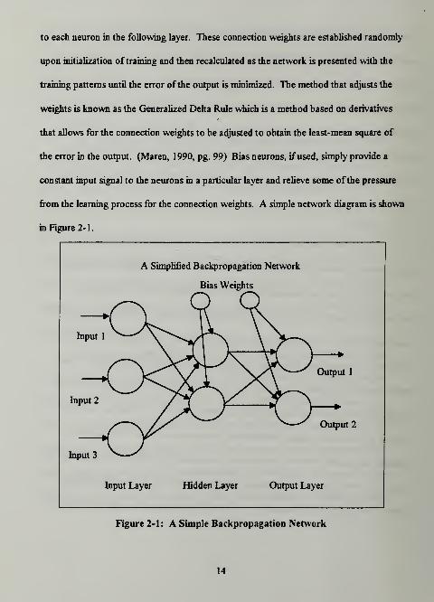
to each neuron in the following layer. These connection weights are established randomly
upon initialization oftraining and then recalculated as the network is presented with the
training patterns until the error ofthe output is minimized. The method that adjusts the
weights is known as the Generalized Delta Rule which is a method based on derivatives
that allows for the connection weights to be adjusted to obtain the least-mean square of
the error in the output. (Maren, 1990, pg. 99) Bias neurons, ifused, simply provide a
constant input signal to the neurons in a particular layer and relieve some ofthe pressure
from the learning process for the connection weights. A simple network diagram is shown
in Figure 2-1.
A Simplified Backpropagation Network
Bias Weights
Input 1
Output 1
Input 2
Output 2
Input 3
Input Layer Hidden Layer Output Layer
Figure 2-1: A Simple Backpropagation Network
14

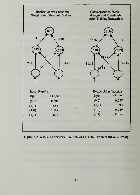
A back-propagation network is capable of generalizing and feature detection
because it is trained with different examples whose features become embedded in the
weights ofthe hidden layer nodes (Maren, 1990, pg. 93). An example ofthe operation of
a neural network is provided by Maren and involves a neural network designed to solve an
XOR classification problem The diagram for this network showing the configuration at
initialization and upon completion oftraining is shown in Figure 2-2 (Maren, 1990, pg.
97).
The example given by Maren is a version ofthe backpropagation network in
which each hidden layer neuron can have a threshold value which is added to sum ofthe
inputs to that neuron before the application ofthe sigmoid transfer function. These
threshold values are found using the same Delta rule that is used to find the connection
weights. During the training process, the connection weights (and threshold values) are
adjusted using the following equation:
Wftnew) = Wftoij) + a * Delta{w^ id) - output activationlevel
where wSjstands for the new and old values ofthe connection weight between node i and
node j, and a is a constant that defines the magnitude ofthe effect ofDelta on the weight.
Delta describes a function that is proportional to the negative ofthe derivative ofthe error
with respect to the connection weight and outputactivationlevel is the output ofthe jth
neuron. This backpropagation of error mechanism allows the weights at all layers to be
adjusted as the training process is performed, including any connections between hidden
layer neurons. (Maren, 1990, pp. 100-101)
15
Initialization with Random Convergence to Stable
Weights and Threshold Values Weights and Thresholds
After Training Interactions
L093J k6.56)
413y\ 85013 34 / \ 13.13
v643} C.rm ^6.06) £7.09)
^37/ i
>a99/
.909 -.441 -11.62 -13.13
j6o \ 12^8 N,
Initial Results: Results After Training
Input Output Input Output
(0,0) 0.590 (0,0) 0.057
(0,1) 0.589 (0,1) 0.946
(1,0) 0.589 (1,0) 0.949
(1,1) 0.601 (1,1) 0.052
Figure 2-2 A Neural Network Example of an XOR Problem (Maren, 1990)
16

An example ofthe operation of a trained network is seen by examining one of
the input combinations in the example provided by Maren (1990) in Figure 2-2. Take the
pattern (0, 1 ). This pattern means that a zero is the input to the bottom left neuron ofthe
trained network and a one is the input to the bottom right neuron. Proceeding up to the
next layer, a vector multiplication ofthe inputs and the connection weights is performed to
determine the inputs to the hidden layer. In this example the hidden layer inputs are
(0*(-l 1.62)H 1*10.99) = 10.99 for the hidden neuron on the left and (0*12.88) +
(1*(-13.13)) = -13.13 for the hidden neuron on the right. The threshold values for these
hidden neurons are added to the inputs and then the sigmoid transfer function is applied
For the hidden neuron on the left, this means the input to the transfer function is
(10.99+(-6.06)) = 4.94. The activation value ofthe input 4.94 when applied to a sigmoid
transfer function that ranges between zero and one is approximately one. For the hidden
neuron on the right, the input to the transfer function is (-13. 13+(-7. 19)) = -20.32. The
activation value when -20.32 is applied to the transfer function is approximately zero. The
hidden layer outputs in this example are one for the left hidden neuron and zero for the
right hidden neuron. The input to the top, or output, neuron is calculated by taking the
product ofthe hidden layer outputs and the connection weights, or (1*13.34)+(0*13.13) =
13.34. The threshold weight ofthe output neuron is added to the input from the hidden
layer to get the input to the transfer function, which in this case is (13.34+(-6.56)) = 6.78.
This number when applied to the transfer function yields a value close to one (0.946),
which is the desired answer. (Maren, 1990, pp. 61-62)
17

3. Applications
Neural networks are currently being used in a variety of applications. Some of
the major uses are in the areas of filtering, image and voice recognition, financial analysis,
and forecasting (Zahedi, 1991, pg. 27). Commercial neural network software is available
from a variety ofvendors. Specialized programmable hardware boards that contain
chipsets that can mimic the operation of a neural network are also available for very
intensive neural network applications. The neural networks in this thesis were developed
using a product from California Scientific Software, Inc. called Brainmaker.
C. GENETIC ALGORITHMS1. History
Nature's capability to find solutions for complex problems through the process
ofnatural selection has fascinated researchers for generations. The ability of organisms to
adapt to their environment by altering their characteristics through mating, which provides
an opportunity for gene crossover as well as an occasional genetic mutation, has proven to
be a powerful technique ofproblem solving. Genetic algorithms were an outgrowth of
early work during the 1950's and 1960's that attempted to combine computer science and
evolution with the hope of creating better programs. In the mid 1960's, John Holland
developed the first genetic algorithms that could be used to represent the structure of a
computer program as well as perform the mating, crossover, and the mutation processes.
Since then, genetic algorithms have grown in popularity and have been applied to a wide
variety ofproblems, especially in the field of engineering design, where optimization
18

involving large numbers of independent variables is a common situation. (Holland, 1992,
pg. 66)
2. Theory
Genetic algorithms are in the simplest definition another method for search and
optimization. However, they differ from traditional methods such as hill-climbing and
random walks in at least four ways (Goldberg, 1989, pg. 7). First, genetic algorithms use
codings ofthe various parameters in a function, not the actual function parameters
themselves. This coding usually consists of fixed-length strings of characters that are
patterned after chromosomes. Each string, or chromosome, then has a fitness value
associated with it which is a measure ofhow well it performs in terms ofthe criteria
defined for the problem Second, genetic algorithms perform highly parallel searches
using a population ofpoints vice a single point. Third, genetic algorithms use the
objective function, or actual payoff information, to determine fitness instead of derivatives
or other information. This capability separates the genetic algorithm from those techniques
that require gradient information about the function to perform their searches. Instead,
the genetic algorithm has the capability to work with the actual function itself Finally,
genetic algorithms use probabilistic rules to make shifts from one generation to the next
instead of deterrninistic rules . (Goldberg, 1989, pp. 7-10)
The easiest way to understand the working ofthe genetic algorithm is to see it in
action. In the following example, similar to the Hamburger Problem presented by Koza
(1992, pg. 18), the genetic algorithm is used to maximize a function. The coding of
19

characteristics in this example is done with the binary digits 1 and and the fitness of each
individual is simply the decimal value ofthe binary representation. The initial population
ofthe first generation, typically referred to as Generation in genetic algorithms, is
randomly generated and shown in Table 2-4.
Table 2-4 Generation of the GA
String # String (X.) Fitness f(X,)
1 101 5
2 Oil 3
! 3 001 1
4 010 2
As can be seen from Table 2-4, the best individual in the initial population has a
fitness of 5, while the worst individual has a fitness of 1 . The population average is 2.75.
After the initial population is evaluated, the next step in the genetic algorithm is the
reproduction and crossover process. The method used to determine which individuals
reproduce is normally determined by a method called fitness-proportionate reproduction
(Koza, 1992, pg. 21).
In fitness proportionate reproduction, candidates for reproduction are selected
for the mating pool by assigning each population member a probability ofreproduction
based upon each population member's fitness. Under this method, highly fit individuals
have higher probabilities for reproduction than lesser fit individuals and the effect ofthis
20

reproduction operation is to increase the average fitness ofthe population. Table 2-5
shows the mating pool for Generation based on fitness-proportionate reproduction.
Table 2-5 Generation Mating Pool Creation
Generation Gen Mating Pool
String Fitness Mating Probability
(Fitness/Sum of Fitness)
Mating
Pool
Fitness
101 5 5/11=0.454 101 5
Oil 3 3/11=0.273 101 5
001 1 1/11=0.090 011 3
010 2 2/11=0.182 010 2
Total 11 Total 15
Best 5 Best 5
Average 2.75 Average 3.75
Table 2-5 shows that the average fitness ofthe population has been increased
but that the best-of-generation-individual fitness remains the same. The second genetic
process, crossover, is what allows new individuals to be formed which may have better
fitness. When the reproduction operation is complete, the crossover operation is
performed by selecting two individuals using a uniform random distribution from the
mating pool Selection through a random distribution is possible since membership in the
mating pool is proportionate to fitness (Koza, 1992, pg. 25). The selected individuals are
separated into fragments by breaking them apart at a randomly selected interstitial point.
The appropriate fragments from the parents are then recombined to form new individuals
that are then tested for fitness. Table 2-6 shows the crossover sequence.
21

Table 2-6 The Crossover Operation
Parent 1 Parent 2
101 on
Crossover Fragment 1(F1) Crossover Fragment 2 (F2)
1- 0-
Remainder 1 (Rl) Remainder 2 (R2)
-01 -11
Offspring 1 (F2+R1) Offspring 2 (F1+R2)
001 111
When the crossover operation is complete, two new individuals have been
created and their fitness is evaluated. The mating pool members not selected for crossover
are copied into the next generation. The number of individuals in the mating pool that
undergo crossover, the crossover rate, is determined in advance by the individual using the
genetic algorithm The mutation operation, if allowed to occur at all also happens during
the reproduction process. In the mutation operation, a single bit is selected for
transformation based upon the probability of mutation, also established in advance by the
individual using the genetic algorithm. (Goldberg, 1989, pg. 14) The results ofthe
reproduction and crossover operations in the simple example are shown Table 2-7.
22

Table 2-7 Generation 1 of the Genetic Algorithm
String Fitness Method of Production
001 1 Reproduction/Crossover
111 7 Reproduction/Crossover
101 5 Reproduction
010 2 Reproduction
Best Fitness 7
Average 3.75
As can be seen from the table, fitness-proportionate reproduction combined with
the crossover operation has improved the average fitness ofthe population and the
best-of-generation fitness (in this case reaching the global optimum). This capability to
search and optimize using adaptive techniques without the requirement for an external
interface to the user is one ofthe strengths of the genetic algorithm.
The engine that gives the genetic algorithm its power is called implicit
parallelism This implicit parallelism manifests itself in what Holland described as the
Fundamental Theorem (Goldberg, 1989, pg. 19) The Fundamental Theorem is derived
from the concept of schemata. A population in a genetic algorithm consists of a set of
strings composed of one's and zero's (a binary representation scheme is commonly used).
Ifthe population consists ofbinary strings, a schema can be thought of as a template that
describes subsets of strings using the notation set {1,0,*}. The asterisk symbol signifies
a "don't care" or "wild card" value. A string with value { 1 10} is then, as an example, a
member of schema {1**} as well as {*!*}, {11*} and {**0}. In fact, a particular string
23

in a population is a member of 2,en6Uwrf-*,rin8
schema. A schema can be thought of as
representing certain characteristics of a candidate solution to the fitness function. As
populations of strings (or chromosomes) proceed from one generation to the next through
the process ofreproduction and crossover, -individuals with greater fitness rise in number
at the expense of lesser fit individuals. Schemata behave in a similar manner. A schema
(or characteristic set) grows at a rate proportional to the average fitness ofthat particular
schema over the average fitness ofthe population. A schema whose average fitness is
above that ofthe population average will be represented in greater numbers in the
succeeding generations. A schema whose average fitness is less than the population
average will see its numbers diminish'. In fact, above average schema will see then-
numbers increase in an exponential manner in succeeding populations. This effect of
simultaneously increasing the fitness ofthe population and promoting the exponential
growth ofbeneficial schemata (or characteristics) through the reproduction operation,
coupled with the crossover operation that creates population diversity through an orderly
exchange of characteristics is what gives the genetic algorithm its implicitly parallel nature.
(Goldberg, 1989, pp. 29-33)
3. Applications
The use ofgenetic algorithms has increased greatly in the past few years as
people have realized the benefits they bring to certain types ofproblems that have resisted
solution by more traditional methods. In one case genetic algorithms were used to
develop control mechanisms for a model of a complex set ofgas pipelines that transport
24

natural gas across a wide area. Having only various compressors and valves with which to
control the gas flow, and with a large time lag between any action and reaction, this
problem had no standard analytic solution. A genetic algorithm was developed by David
Goldberg at the University of Illinois that was capable of "learning" the control procedure.
In another case, Lawrence Davis used genetic algorithms to design communications
networks that maximized data flow with a minimum number of switches and transmission
lines. General Electric is currently using genetic algorithms in the design ofnew
commercial turbofan engine components. Using a genetic algorithm, General Electric
engineers were able to reduce the time required to improve the design of an engine turbine
from weeks to days. This is notable since there are at least 100 variables involved in a
turbine design as well as a large number of constraints. (Holland, 1992, pg. 72-73)
Goldberg's text lists additional uses ofgenetic algorithms ranging from medical imaging to
biology to the social sciences (Goldberg, 1989, pg. 126). There are currently several
conferences, both national and international, devoted to the discussion ofgenetic
algorithms.
D. GENETIC PROGRAMMING1. History
Genetic programming is an exerting new field in computing pioneered by John
Koza of Stanford University in the late 1980's. Koza, in his text Genetic Programming:
On the Programming ofComputers by Means ofNatural Selection, describes the core
concept ofhis technique as being the search for a computer program of a given fitness
25

from the space of all possible computer programs using the tools ofnatural selection. This
approach is different from more traditional artificial intelligence techniques in that for any
particular problem using traditional techniques, such as neural networks, the goal is
usually to discover a specialized structure that provides a certain output given certain
inputs. Koza reframes this statement by saying what we truly want to discover is a certain
computer program that will produce the desired output from a given set ofinputs. Once
the problem is refrained as that of finding a highly fit program within the space of all
possible programs, the problem is reduced to that of space search. (Koza, 1992, pg.2)
The technique ofgenetic programming is not the first attempt at using
computers to try to generate programs. Researchers since the 1950's have attempted
using various methods to generate programs ranging from blind random search to asexual
reproduction and mutation. More recently, researchers in the genetic algorithm field have
attempted to use genetic algorithms to generate programs by using ever more specialized
chromosome representation schemes or by using a special type ofgenetic algorithm
known as a classifier system to generate programs based on if-then rules (Koza, 1992, pp.
64-66). Koza is the first researcher, however, to develop an appropriate representation
scheme and methodology for applying natural selection techniques to the problem of
program generation.
2. Theory
The concept of a "highly fit" computer program as a solution to a particular
problem is disturbing to most people at first. We are accustomed to the idea of a
26

computer program being either "right" or "wrong" when applied to a particular problem.
Koza counters this sentiment and other similar sentiments by saying that the process of
natural selection is neither "right" nor "wrong" but that nature supports many different
approaches to the same problem, all ofwhich have a certain "fitness". The key to nature's
approach, according to Koza, is that form follows fitness (Koza, 1992, pp. 1-7). The
requisite tools used in Koza's approach are a well-defined function representation scheme,
a method for generating an initial random population ofprograms, a fitness measurement
technique, and a procedure for applying genetic operations to the members ofthe
population.
The representation scheme chosen by Koza for genetic programming is based on
a type of structure known as a symbolic expression, or S-expression. Since this type of
structure is a key component ofthe programming language LISP, this language was
chosen as the platform for developing genetic programming. It is not a requirement to use
this language for genetic programming, but it has many features that facilitated the
development ofthis technique. (Koza, 1992, pp. 70-71) An example of a LISP
S-expression is shown in Figure 2-3.
As can be seen from Figure 2-3, a LISP S-expression is equivalent to the parse
tree for a particular program, which in this case is l*(2+3). The ability ofLISP structures
to serve as both data (to be manipulated) and programs (to be executed) is another ofthe
reasons LISP was chosen as the language for the development ofgenetic programming.
(Koza, 1992, pg. 71)
27

Figure 2-3 A LISP S-expression
In genetic programming, these LISP S-expressions are composed of structures
that are derived from a predefined function set and terminal set. The function set consists
ofwhatever domain-specific functions the user feels are sufficient to solve the problem
and the terminal set is the arguments that the functions are allowed to take on (Koza,
1992, pg. 80). For instance, the function set may be comprised ofmathematical,
arithmetic, or boolean operators while the terminal set is usually comprised ofvariables
from the problem domain and an unspecified integer or floating-point random constant.
Since it is impossible to determine in advance what the structures will look like, it is
necessary to ensure in advance that each function possesses the property of closure (Koza,
1992, pg. 81). The closure property requires that the allowable arguments for any
function be well-defined in advance to prevent the function from taking illegal arguments.
While this may seem like an imposing task, it is usually not a serious problem and is easily
rectified by prior planning ofthe function definitions. As an example, division by zero is
undefined. Ifthe division operator is a member ofthe function set, then by defining a
28

special division operator in advance that handles this special case, it is possible to ensure
closure on this function. (Koza, 1992, pg. 82)
Once the representation scheme is defined, the initial program structures can be
generated (Koza, 1992, pg 91). In Koza's method, the initial structures are generated
randomly using a combination oftwo techniques, "full" and "grow". The root, or
beginning, ofone ofthe LISP S-expressions, or trees, is always a function, since a root
that consisted of a terminal would not be capable taking any arguments. Once the root
function is selected, a number of lines, equivalent to the number of arguments the function
requires, are created which radiate away from the function. The endpoints ofthese lines
are then filled by a selection from the combined set of functions and terminals. If another
function is selected as an endpoint, the selection process continues onward until the
endpoints consist ofterminals. There is a preset maximum depth that trees may attain.
The terms "full" and "grow" as mentioned above refer to the depth ofthe trees. In the
"full" method, all trees filled until they are at the specified maximum depth. In the "grow"
method, the trees are ofvariable depth. In practice, Koza recommends an approach called
"ramped half-and-half' that combines these two approaches (Koza, 1992, pp. 91-92).
Koza additionally recommends that each structure generated for the initial random
population be checked for uniqueness to ensure a range of diversity ofgenetic material
(Koza, 1992, pg. 93). Figure 2-4 gives a graphical representation ofthe creation ofan
individual in the initial population.
29

Figure 2-4 Graphical Representation of Tree Generation
Once the initial population is generated the fitness ofthe individuals in the
population must be determined. There are a number of different ways to compute fitness,
but in general, most ofthe methods involve measuring the performance of a member ofthe
population in relation to a predetermined set of fitness cases. As a guide, the set of
fitness cases must be representative ofthe entire domain since they will serve as the basis
for achieving a generalized result (Koza, 1992, pg. 95).
After the fitness ofthe initial random population is calculated, the genetic
operations ofreproduction and crossover are performed. In genetic programming, the
reproduction and crossover operations are designed to happen as separate events rather
30

than as parts of a two-step process as with the genetic algorithm. Reproduction occurs by
copying an S-expression from one generation to the next. Candidates for reproduction
are selected by using the fitness-proportionate method or a second method known as
tournament selection. In tournament selection, a specified number ofpopulation members
are randomly selected with replacement. The individual with the best fitness is then
reproduced in the next generation. The sampling with replacement is what ensures that
fitter individuals survive into succeeding generations. (Koza, 1992, pg. 100)
The crossover operation in genetic programming is more complex than that of
the genetic algorithm due to the differences in the structure ofthe population members.
The crossover candidates are selected using the same method chosen for reproduction.
This ensures that crossover occurs between individuals in a manner proportionate to then-
fitness. After two individuals have been selected a separate random number is chosen for
each individual which corresponds to a point in each structure. It is at these points that
the crossover operation takes place by swapping subtrees. (Koza, 1992, pg. 101) Figure
2-4 shows an example ofthe crossover operation. The previously described property of
closure on the function set ensures that any resulting S-expressions will be legitimate
program representations. Since the points selected for crossover are most likely to be at
different levels in each structure there are a variety of situations that may result. (Koza,
1992, pg. 103) An individual may reproduce with itself and produce two totally new
structures. Ifthe crossover point happens to be at the root ofon S-expression, that entire
S-expression will become a subtree on the other parent. Ifthe root is selected in both
31

Parent 1 Parent 2
Crossover
Points
Child 1Child 2
Figure 2-5 The Genetic Programming Crossover Operation
parents, they are both just copied into the next generation. The constraint on maximum
structure depth is the only major limit on the crossover operation.
The third genetic operation of mutation is rarely used in genetic programming.
The normal argument for its use, in order to promote genetic diversity, is not as important
when one considers the variety of structures with different sizes and orientations that are
likely to be obtained from the crossover process. Additionally, when the crossover points
in both parents correspond to endpoints in each structure, the effect is similar to a
mutation at a single point. (Koza, 1992, pg. 106)
32

3. Applications
Due to its relative youth as a technique, applications using genetic programming
are currently confined to mostly experimental problems. Koza does present in his text a
copious amount ofexamples of applying his technique to a wide range ofproblems,
including symbolic regression, game playing strategies, decision tree induction, and
artificial life (Koza, 1992, pg. 12-14). In each case, a domain specific function set with
the proper closure was determined in advance. Once the function set and the appropriate
fitness measure was specified, all ofthe problems proceeded in the identical manner using
a domain-independent implementation ofthe mechanical operations of evolution. An
initial population was generated at random and the genetic operations ofreproduction and
crossover were used to create succeeding generations. Koza was able to show via
empirical methods that genetic programming succeeded in each case to find a solution that
satisfied the appropriate fitness measure (Koza, 1992, pg. 4). This ability to solve
problems over a wide variety ofdomains by using a domain-independent method for
searching the space ofpossible computer programs to find an individual computer
program is what makes genetic programming an exciting new method ofdiscovery (Koza,
1992. pg. 8).
33

m. DESIGN OF EXPERIMENTS
A. DATA SELECTION.
The COCOMO data set used for training and testing the machine learning techniques
examined in this thesis is drawn from pages 496 and 497 ofBoehm's book, Software
Engineering Economics. The sixty-three projects used to develop the three versions of
COCOMO are summarized in this data base. This data includes the project type, year
developed, the development language, the values ofthe 15 cost drivers, the development
mode, and the various COCOMO estimates. The Kemmerer project data was provided by
the author in electronic form and is included in Appendix C. The experimental approach
taken for each machine-learning technique consisted of a two-step process that required a
different training and testing data set for each step. The first step used only the
COCOMO data partitioned into training and testing data sets. The second step consisted
ofusing the COCOMO data for training and the Kemmerer data for testing. The
partitioning ofthe COCOMO data set in the first step required two tradeoff
considerations.
The first tradeoffinvolved the size ofthe training and testing data sets. Machine
learning methods perform at their best when they have a large amount of data available for
training that is representative ofthe population, or problem domain. In fact a good
guideline is more is always better. However, there are only 63 projects available in the
COCOMO data base in the text. In this case, choosing to use too much data for training
34

reduces the number of data sets available for testing and trivializes the results beyond a
certain point. Alternatively, choosing too little data for training reduces the effectiveness
ofthe machine learning techniques. A balance was struck by deciding to break the data
into thirds, with two-thirds to be used for training and one-third to be used for testing.
This was accomplished by transcribing the data set from the text into a Quattro Pro
spreadsheet and then sorting the projects by size and type. Once the data was sorted in
this manner, a random number between one and three was assigned to each project. The
data was then partitioned into groups based on the random number assigned and each
group was analyzed. This cursory analysis showed that for each group the mean project
size in thousands of delivered source instructions (KDSI), the average year of
development, and the development mode proportions were roughly similar, indicating a
reasonable distribution. After this analysis, 42 ofthe projects were identified as the
training set and 21 projects were identified as the testing set. These data sets are included
in Appendix D. The same training and testing sets were then used for all ofthe machine
learning techniques examined. The composition ofthe training and testing data sets for
each set ofexperiments was also kept as identical as possible and consisted ofthe project
size, annual adjustment factor, development mode, and the fifteen COCOMO cost drivers,
with limited exceptions.
One effect ofpartitioning the data in this manner is that the testing data set may not
be completely characteristic ofthe "population". Some testing set projects contained
some cost driver values that were not contained in the training data set. This situation
35

describes the second tradeoff Hand selecting the data to ensure that every cost driver
value represented in the data base was in the training set was initially considered but
rejected for two reasons. First, it would probably be meaningless when considering that
there are, at a minimum, four values for each cost driver. For fifteen cost drivers this
means there are at least 4" possible combinations of cost drivers, and there are only 63
projects in our data set. Secondly, on a more practical basis, several ofthe cost driver
values are only represented once in the project data base, so ifthey were included in the
training data there would be no way of examining the effectiveness ofthis measure.
Therefore, there appeared to be no benefit in ensuring that every cost driver value was
fully represented in the training set.
B. NEURAL NETWORK PROCEDURES1. Neural Network Software
The software used to develop the neural networks in this thesis is BrainMaker
Professional v2.5, which is designed and marketed by California Scientific Software, Inc.
This software is a DOS-based product manufactured for use on IBM-compatible personal
computers. BrainMaker is designed to construct, train, test, and run back-propagation
neural networks. It is a menu-driven program that provides the user a large range of
control over the design and operation of a neural network. BrainMaker comes with an
extensive manual as well as a companion program called NetMaker which can be used to
prepare the data files needed by BrainMaker. All ofthe files used by BrainMaker are in
standard ASCII format, so they can be prepared using most any text editor ifthe user so
36

desires, although using the NetMaker program speeds up the process since it helps
automate the generation ofBrainMaker's inputs.
BrainMaker requires two files at a minimum to train. The first file is the
network definition file, which tells BrainMaker the key network parameters, such as the
number of input and output neurons, the number ofhidden layers and hidden neurons, the
input and output data definitions and ranges, the learning rate, and the type oftransfer
function the neurons will use. An example of a network definition file is shown in Figure
3-1. The second file that BrainMaker requires is the fact file. This is the file that contains
the data the network will use for training. This file consists of alternating rows of data,
with the first row representing one input set and the second row representing one output
set. An example of a fact file is contained in Figure 3-2. Additional input files that may be
included are a testing fact file and a running fact file. The testing fact file consists of
alternating rows ofinput and output data not included in the training fact file. This data
may be used during the training process to judge the prospective performance ofthe
network at user-defined intervals during the training process. When a testing fact file is
specified, BrainMaker pauses at the specified interval and tests the current network
configuration using the facts in the testing fact file. The results ofthese tests along with
some associated error statistics are written to an output file. The training statistics for
each run may also be written to a separate file if this option is activated. The running fact
file provides the user with the capability to test the trained network with new sets ofinputs
in a batch manner and write the results to an output file in a user-specified format.
37

2. Neural Network Design
The neural network design and training process is very iterative. Since any
network configuration will learn some training facts to the user-specified level oftolerance
during the training process it is important to have a strategy for determining a broadly
effective configuration when beginning the network design process.
input number 1 20
output number 1 1
hidden 16 19
filename trainfacts c:\brain\test\cltrain.fct
filename testfacts c:\brain\test\cltrain.tst
learnrate 0.9000 50 0.75 75 0.6000 90 0.5000
learnlayer 1.0000 1.0000 1.0000
traintol 0.1000 0.04 0.8000 100
testtol 0.2000
random 5.0
maxruns 500
testruns 1
function hidden 1 sigmoid 0.0000 1.0000 0.0000 1.00000
function hidden2 sigmoid 0.0000 1.0000 0.0000 1.00000
function output sigmoid 0.0000 1.0000 0.0000 1.00000
dictionary input LOGJCDSI AAF RELY DATA CPLX TIME STOR VTRT TURNACAPAEXP PCAP VEXP LEXP MODP TOOL SCED E ORG SDdictionary output LOG_MMACscale input minimum0.47712 0.43000 0.75000 0.94000 0.70000 1.00000 1.00000 0.87000 0.87000
0.71000 0.82000 0.70000 0.90000 0.95000 0.82000 0.83000 1.00000 0.00000
0.00000 0.00000
scale input maximum2.66651 1.00000 1.40000 1.16000 1.30000 1.66000 1.56000 1.30000 1.15000
1.19000 1.29000 1.42000 1.21000 1.14000 1.24000 1.24000 1.23000 1.00000
1.00000 1.00000
scale output minimum0.77815
Figure 3-1: A sample network definition file
There is no way to know which network configuration will be the most
successful in learning the data prior to the training process. At best, some authors
38

recommend general guidelines for network design that can serve as a starting point. The
makers ofBrainMaker suggest first that there is no little reason to have a network with
more than two hidden layers (BrainMaker, 1992, pg. 14-4). They state in their manual
that they have never observed a network with more than two hidden layers that could not
also be trained on just two layers. As for the number ofneurons in the hidden layers, there
are two suggestions. The makers ofBrainMaker (1992) suggest using the sum ofthe
input and output neurons divided by two, while the authors Eberhart and Dobbins (1990)
suggest using the square root ofthe sum ofthe input and output neurons phis a couple.
Both ofthese guidelines are based on empirical observations, not any underlying principle.
In the end, it is necessary to experiment with a variety ofnetworks to determine a
successful configuration. This is probably the most time-consuming portion ofthe design
process but BrainMaker has a method for automating this process to a certain extent.
farts
1.62324 0.96 14 1.08 1.3 1.48 1.56 1.15 0.94 0.86
0.82 0.86 0.9 1 0.91 0.91 1 [ E2.78175
2
1.36172 0.96 1.15 1.08 1 1.06 1 1 0.87 1 1
1 1 1 0.91 1.1 1.23 [ E2.36172
1.79239 0.81 1.4 1.08 1 1.48 1.56 1.15 1.07 0.86 0.82
0.86 1.1 1.07 1 1 1 [ E3.02653
4
1.57978 1 1.15 1.16 1.3 1.15 1.06 1 0.87 0.86 1
0.86 1.1 1 0.82 0.91 1.08 [ E2.7185
Figure 5-2 A Sample BrainMaker Fact File
39

3. Preparations for Training
A key aspect in preparing to train a network is data preparation. Due to the
nature ofneural networks and the way that the training tolerance is calculated, it is
necessary to pay particular attention to the way the data is presented to the network.
First, all input variables should vary over a roughly similar range between the minimum
and maximum values. The reason for this is fairly straightforward. Since every input is
connected to each neuron in the first hidden layer, a single input that varies over a large
range can tend to "drown out" the other inputs, diminishing their contribution. Secondly,
since the inputs and outputs to the network are all normalized, data that varies over a wide
range reduces the ability ofthe network to distinguish small changes. For example, if a
significant portion of a particular piece of data ranges between 500 and 600 while a few
values range between 10 and 20, the network will have difficulty determining the
difference between 10 and 20. As a rule ofthumb, smaller changes are better. This
becomes particularly important when understanding the concept ofnetwork training
tolerance.
Tolerance is the statistic used to determine the level ofprecision to which the
network trains. Tolerance is expressed as a percentage ofthe difference between the
minimum and maximum output values. As an example, ifthe minimum output is 10 and
the maximum output is 1000, then a tolerance of 0. 1 means that any network output that
falls within 0. 1*( 1000- 100) = 90 ofthe actual output value will be considered correct by
the network. Therefore, ifthe output training values vary over a large range, the accuracy
40

ofthe network will be diminished. This required two transformations to the COCOMO
data for use with the neural network. Since the KDSI values and the actual man-months
vary over a large range, logarithms ofthese two values were used, which greatly reduced
the difference between the minimum and maximum values and increased the ability ofthe
network to learn and predict project effort.
4. Automating the Training Process
BrainMaker has an option which allows the user to specify a range ofnetwork
hidden layer configurations, as well as other parameters, that can be tested in a variation of
a brute force attack (BrainMaker GTO, 1993, pg. 5). This option was used to test three
ranges ofnetwork configurations that were used in an iterative process to search for the
best-performing network configurations. The three ranges tested are summarized in Table
3-1:
Table 3-1 Network Ranges Tested
Number of Hidden Neurons Number of Layers
ItolO 1 and 2 hidden layers
10 to 20 1 and 2 hidden layers
15 to 25 1 and 2 hidden layers
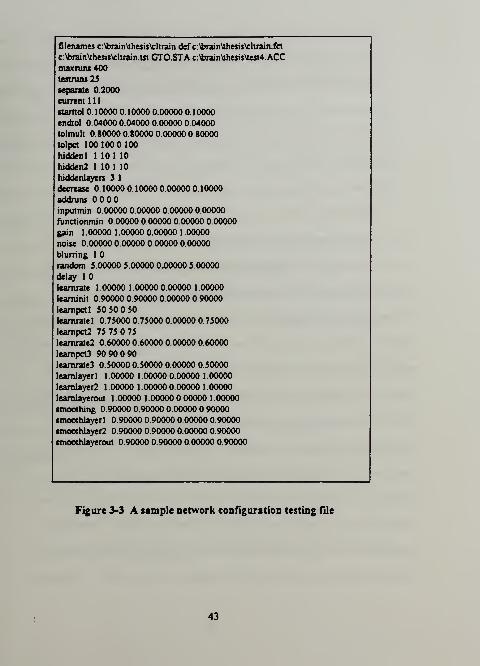
The use ofthis option requires the user to create an additional input file beyond
the usual training, testing, and definition files. This setup file contains all the network
configuration parameters and the ranges ofthose that are being varied. In this study, the
only parameters varied were the number ofneurons and hidden layers, since these two
factors have the greatest effect on overall network performance. The remaining network
41

parameters (which deal mostly with the learning rate associated with the Deha rule) were
fixed with the exception oftraining tolerance, which was allowed to decrease in a stepwise
pattern from 0. 1 to a Hmh of 0.04. The stepwise decreases in tolerance are triggered
when the network learns all the training facts at the current training tolerance. The testing
tolerance was specified as 0.2. An example ofthe setup file for this option is shown in
Figure 3-3:
The training and testing data files consisted ofthe COCOMO data modified as
mentioned previously by changing the KDSI and effort values into logarithmic values.
There were 42 training patterns and 21 testing patterns. The network definition file
consisted of a generic network definition file that provided the ranges ofthe input values
and the variable names, similar to the file shown in Figure 3-1.
Once the three ranges of configurations had been tested and all ofthe results
written to three output files, the top performing networks were selected. The selections
were made by reading all ofthe output files into Quattro Pro for Windows spreadsheets
and sorting the results based on the number of correct outputs for both the training and
testing data sets. After the sorting process, the networks shown in Table 3-2 were chosen
for further training at a more detailed leveL The choice ofthis iterative process was based
upon several factors that mainly involved hardware and software constraints. The
hardware constraint concerned the disk space required to save the testing results. In the
hutial round oftesting, the statistics for the testing data set were written to disk every 25
runs. Each ofthese runs took approximately four to five hours on a 33 MHz 486
42
filenames c:^wain\thesis\dtrain.def c:\brain\thesis\cltrain.fct
c:\brain\thesis\cltrain.tst GTO.STA c:\brain\thesis\test4.ACC
maxruns 400testnins25
separate 0.2000
current 1 1
1
ftarttol 0.10000 0.10000 0.00000 0.10000
endtol 0.04000 0.04000 0.00000 0.04000
tolmult 0.80000 0.80000 00000 0.80000
tolpct 100 100 100
hiddenl 1 10 1 10
hidden2 1 10 1 10
hiddenlayers 3 1
decrease 1 0000 1 0000 00000 1 0000
addnins 00 00inputmin 0.00000 0.00000 0.00000 00000
functionmin 0.00000 0.00000 0.00000 0.00000
gain 1.00000 1.00000 0.00000 1.00000
noise 0.00000 0.00000 0.00000 0.00000
blurring 1
random 5.00000 5.00000 0.00000 5.00000
delay 10learnrate 1 00000 1 00000 00000 1 00000
learninit 0.90000 0.90000 0.00000 0.90000
learnpctl 50 50 50
learnratel 0.75000 0.75000 0.00000 75000
learnpct2 75 75 75
leamrate2 0.60000 0.60000 0.00000 0.60000
leampct3 90 90 90
learnrate3 0.50000 0.50000 0.00000 0.50000
learnlayerl 1.0)000 100000 0.00000 1.00000
learnlayer2 1.00000 1.00000 0.00000 1.00000
learnlayerout 1.00000 1.00000 0.00000 1.00000
smoothing 0.90000 0.90000 0.00000 0.90000
smoothlayerl 0.90000 0.90000 0.00000 0.90000
smoothlayer2 0.90000 0.90000 0.00000 0.90000
smoothlayerout 0.90000 0.90000 000000 0.90000
Figure 3-3 A sample network configuration testing Tile
43

Table 3-2 Top Network Configurations
First Hidden Layer Neurons Second Hidden Layer Neurons
5 8
8 9
10 11
16 19
It 15
24 25
computer and took approximately 300 kilobytes of disk space. Saving the results for
every run would have risked filling all the disk space available on the disk and risked
crashing the computer while unattended, which would have wasted a training run.
Additionally, the resulting data files would have been too large to load into a spreadsheet
in order to perform the sorting operations. This is the reason the training was broken into
two cycles, with the goal ofthe first cycle being to identify the networks with the best
performance at a macro level. The criteria that was used to determine which networks to
choose for further training was based on which networks correctly predicted all 21
projects in the testing data set at some point during their training period. Six network
configurations met this criteria. Once these six best network configurations were
identified, the second round oftraining was performed. For this training cycle, network
definition files were created for each ofthe six configurations. AD parameters in these
definition files were identical except for the number ofneurons in the two hidden layers.
For these networks, the maximum number oftraining runs was set to 500. A run is this
44

sense is defined as a pass through the entire training data set in which fitness statistics are
accumulated for the current configuration and weight vector set. The COCOMO training
and testing files were provided as inputs. Training and testing statistics for all 500 runs
were accumulated in separate files for each ofthe six configurations. Once this cycle of
training was over, the testing and training statistics files were again read into Quattro Pro
for Windows spreadsheets and analyzed to determine the optimum number oftraining runs
for each ofthe six configurations. This optimum point was based on the run where all 42
projects in the training data were correctly predicted and the network training tolerance
was at a minimum for the training cycle. When this point was determined for each
network, the training process was repeated from the beginning up to this optimum
performance point. The analysis ofneural network performance is based upon the results
obtained from these final versions ofthe six networks. The definition files for these
networks are shown in Appendix E.
This entire network training process starting with the six network configurations
was repeated a second time in order to test the performance ofthe neural network on a
data set separate from Boehm's COCOMO data set. In this second round of
experimentation, all ofthe 63 COCOMO projects were used as the training set, and the IS
projects that make up the Kemmerer data set were used as the testing set.
45

C. GENETIC ALGORITHM PROCEDURES1. Genetic Algorithm Goal
The goal ofthe second group ofexperiments in this thesis was to use a genetic
algorithm to determine an optimum set of.values for the cost drivers, coefficients, and
exponents for the Intermediate COCOMO model. In this group ofexperiments the inputs
to the genetic algorithm included the Intermediate COCOMO model structure,
MM = Effort Adjustment Factor*COEFF*(Adjusted KDSI)**EXP
and the partitioned COCOMO data with two modifications. The first modification to the
COCOMO training and testing data set prior to using the genetic algorithm consisted of
multiplying the annual adjustment factor and KDSI values together to obtain the adjusted
KDSL This action was taken since the Annual Adjustment Factor provided no additional
information to the genetic algorithm process in the absence ofinformation on how it was
derived. The second modification consisted of expressing the cost drivers by their literal
values, such as HIGH, LOW, or NOMINAL, vice their numeric values.
2. Genetic Algorithm Software
The genetic algorithm software package used was GAucsd 1.4, a C-language
genetic algorithm developed by Nicol Schraudolph ofthe University of California, San
Diego, based on previous work by John Grefenstette ofthe Naval Research Laboratory.
The uncompiled C code for GAucsd 1.4 is publicly available via anonymous ftp on the
Internet and can be adapted to any machine that has a C compiler. In this case the target
46

platform was a Sun workstation The choice ofGAucsd 1.4 was based on its availability
and ease ofuse. This package is well-designed in that the user has only to supply a
chromosome structure and a fitness function (written in C) that defines the problem.
GAucsd 1.4 provides the rest ofthe functionality required in a genetic algorithm, such as
population initialization, crossover, and mutation. GAucsd 1.4 also provides an awk
language macro that integrates the user defined fitness function and adds in the code
required to implement the genetic algorithm operations. This design feature relieves the
user ofthe task ofcode integration. (Schraudolph and GrefTenstette, 1992, pp. 9-12)
3. GAucsd Preparation
The chromosome structure defined in the genetic algorithm fitness function used
in this study consisted of a string of 96 numbers that represented all ofthe cost driver
values, along with the coefficients and exponents for all three project development modes.
Since there are a maximum of six values for each cost driver and a total of fifteen cost
drivers, the first 90 numbers represented the cost drivers. Although most cost drivers
have less than six values, a total of six values were reserved for each driver. This aided in
the structure ofthe problem by allowing the indexing process to operate as ifthe first 90
numbers represented a pseudo 6x15 array. The excess cost driver values in no way
impeded the functionality ofthe genetic algorithm. The numeric values derived by the
genetic algorithm were substituted for the literal values in the COCOMO training set
which were stored as index values in a C table structure. These first 90 values were
allowed by the fitness function to range from 0.5 to 2.0. The 91st through 93rd numbers
47

represented the coefficients for each development mode and the 94th through 96th
numbers represented the exponents for each development mode. These last six values
were allowed by the fitness function to range from 0.0 to 4.0. The choice ofthese ranges
was somewhat arbitrary but allowed for a .greater range ofvalues than those expressed in
Boehm's Intermediate COCOMO model. The actual fitness measure for each member of
the population was initially the average relative error ofthe actual effort in the COCOMO
training data set versus the estimated effort calculated by the fitness function. This
estimated effort was calculated using the Intermediate COCOMO model as a template.
The genetic algorithm derived numeric values for the literal cost driver values, along with
the coefficient and exponent values appropriate for each project's development mode then
were used as inputs into the Intermediate COCOMO model. The capability to impose
constraints on the values generated by the genetic algorithm was also provided and is
expanded upon later. The GAucsd user-defined fitness function is shown in Appendix F
4. Initial Genetic Algorithm Benchmarking
Along with the user-defined fitness function, the other input to the GAucsd 1.4
program is the default file that specifies population size, crossover rate, mutation rate, and
number of generations. The first step in using the genetic algorithm centered on finding an
effective population size and crossover rate to use with the 960 bh chromosome. This
was accomplished by a series oftest runs using various population sizes and crossover
rates while keeping mutation rate and number ofgenerations constant. The test runs are
summarized in Table 3-3.
48
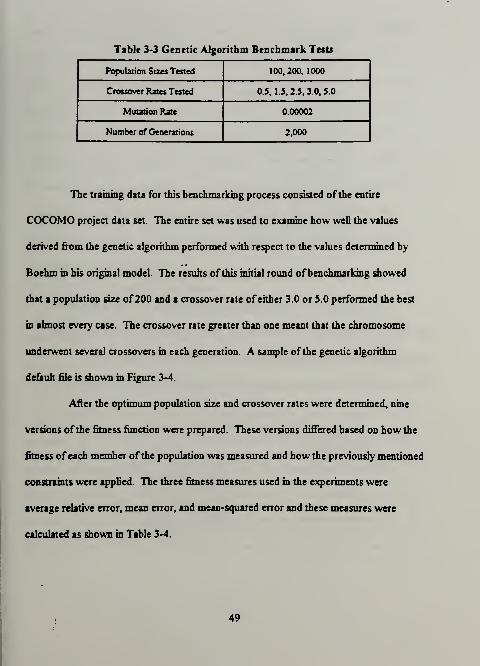
Table 3-3 Genetic Algorithm Benchmark Tests
Population Sizes Tested 100, 200, 1000
Crossover Rates Tested 0.5,1.5,2.5,3.0,5.0
Mutation Rate 0.00002
Number of Generations 2,000
The training data for this benchmarking process consisted ofthe entire
COCOMO project data set. The entire set was used to examine how well the values
derived from the genetic algorithm performed with respect to the values determined by
Boehm in his original model. The results of this initial round ofbenchmarking showed
that a population size of200 and a crossover rate of either 3.0 or 5.0 performed the best
in almost every case. The crossover rate greater than one meant that the chromosome
underwent several crossovers in each generation. A sample ofthe genetic algorithm
default file is shown in Figure 3-4.
After the optimum population size and crossover rates were determined, nine
versions ofthe fitness function were prepared. These versions differed based on how the
fitness ofeach member ofthe population was measured and how the previously mentioned
constraints were applied. The three fitness measures used in the experiments were
average relative error, mean error, and mean-squared error and these measures were
calculated as shown in Table 3-4.
49
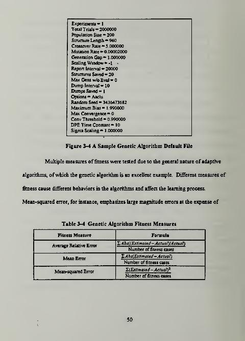
Experiments « 1
Total Trials - 2000000
Population Size 200
Structure Length 960
Crossover Rate 5.000000
Mutation Rate * 0.00002000
Generation Gap - 1.000000
Scaling Window «-l -
Report Interval * 20000
Structures Saved « 20Max Gens w/o Eva!
Dump Interval 10
Dumps Saved -
1
Options Aaclu
Random Seed - 3436473682
Maximum Bias 1 .990000
Max Convergence *Conv Threshold «= 0.990000
DPE Time Constant - 10
Sigma Scaling - 1 .000000
Figure 3-4 A Sample Genetic Algorithm Default File
Multiple measures of fitness were tested due to the general nature ofadaptive
algorithms, ofwhich the genetic algorithm is an excellent example. Different measures of
fitness cause different behaviors in the algorithms and affect the learning process.
Mean-squared error, for instance, emphasizes large magnitude errors at the expense of
Table 3-4 Genetic Algorithm Fitness Measures
Fitness Measure Formula
Average Relative ErrorZAbs((Estimated-Actual)/Actual)
Number of fitness cases
Mean ErrorZAbs(Estimatcd-Actual)
Number of fitness cases
Mean-squared Error ^Estimated -Adual)2
Number of fitness cases
50

smaller magnitude errors. This type ofbehavior caused the genetic algorithm to focus on
learning the larger software projects that had large errors at the expense ofthe smaller
projects. This behavior led to poor results. Mean error reduced this tendency to a degree,
but the best learning performance was found when using average relative error. In these
experiments, this fitness measure equalized the effort the genetic algorithm expended
learning all ofthe projects since error was expressed as the average percentage difference
between the estimated value and the actual value A secondary observed benefit ofthis
measure was that both mean error and mean-squared error were also minimized when
using this fitness measure even though neither ofthese fitness measures were explicitly
expressed in the fitness function.
5. Genetic Algorithm Constraints
The final aspect ofthe various fitness functions involved the imposition of
various degrees of constraints on the values generated by the genetic algorithm. An
inspection ofBoehm's COCOMO cost driver, coefficient, and exponent values reveals
certain patterns or constraints. For example, in the case ofthe COCOMO exponents, the
magnitude ofthe exponent increases as the mode shifts from organic to semidetached to
embedded. Conversely, the coefficient decreases as the same mode shifts occur. Similar
patterns can be seen in the values ofthe cost drivers. When inspecting the cost driver
table, the magnitude ofthe first seven cost drivers increases when moving from a value of
Very Low to a value ofExtra High. The opposite movement occurs in drivers eight
through fourteen. In this case the magnitude ofthe driver decreases as the value shifts
51

from Vciy Low to Very High. The value ofthe final cost driver, required development
schedule (SCED), moves in a high-low-high manner as the value shifts from Very Low to
Very High. These patterns can be interpreted as constraints that the cost driver values
should obey. To test whether or not these constraints added to the ability ofthe genetic
algorithm to learn the project data and find an optimal set ofvalues, these constraints were
embedded in three versions ofthe fitness function. In the first version, no constraints were
placed on the order ofthe cost drivers, exponents, or coefficients. In the second version,
penalty measures were introduced on the cost drivers so that ifthe previously identified
patterns in the first 14 cost drivers (SCED was allowed to vary without constraint) did not
appear in the chromosome, the fitness ofthe individual was penalized based upon the
degree ofnon-compliance. In the final version ofthe constrained fitness function, penalty
measures were introduced on the generation ofthe exponents and coefficients as well as
the cost drivers.
6. The Genetic Algorithm Testing Process
The nine fitness functions used for training the genetic algorithm were
constructed using the three measures offitness and the three constraint levels previously
described. Testing was performed using a population size of200 and crossover rates of
3.0 and 5.0 with the number ofgenerations set at 5000 for all tests. There were 18 total
tests and each test took approximately two to four hours on a Sun workstation. The top
twenty chromosomes in each test were saved to an output file and read into a Quattro Pro
for Windows spreadsheet. The chromosome values with the best fitness in each run were
52

translated into their associated COCOMO model values using a previously constructed
series oflinked spreadsheets. This table oftranslated COCOMO model values was then
linked to the test data set in such a manner as to allow for automatic updating ofthe test
data and its associated performance measures whenever new chromosome data was pasted
into the spreadsheet. The results of all 18 tests were processed in the same manner.
A slightly different procedure to that previously described was used when the
genetic algorithm was trained using all 63 COCOMO projects and tested with the
Kemmerer project data. In this case, the best parameter set from the original genetic
algorithm benchmarking tests was used along with the full range of constraints in the
fitness function. The use of all ofthe constraints was based upon the results observed in
the first phase oftesting. The number of generations was increased from the
benchmarking level of2000 to 5000. The top twenty chromosomes from this run were
again saved to an output file that was loaded into a spreadsheet holding the Kemmerer
data The performance ofthe genetic algorithm with respect to the Kemmerer project set
was then calculated.
D. GENETIC PROGRAMMING PROCEDURES1. Genetic Programming Software
The goal ofthe final group ofexperiments in this thesis was to test the ability of
genetic programming to derive an explicit cost estimation model given only the COCOMO
data and a fitness function. The genetic programming software used was SGPC: Simple
Genetic Programming in C by Waiter Alden Tackett and Aviram CarmL This software
53

is based on the original LISP code published by Koza in his book and is available via
anonymous ftp from the Santa Fe Institute and the University ofTexas. This software
provides all the functionality required to apply genetic programming to a variety of
problem domains. The genetic operations ofpopulation initialization, crossover,
reproduction, and mutation are fully supported by this software. The user is only
responsible for defining functions specific to the problem at hand, ensuring closure ofthe
functions, and providing the appropriate fitness function and terminal set. This software
also has the capability to train and test simultaneously, which reduces the
post-experimental processing ofthe output expressions. Due to the memory requirements
and CPU intensive nature ofthis application, the target platform for this application was a
Sun workstation.
2. Genetic Programming Preparation
Preparation for the genetic programming process using the SGPC software
involved five steps. In the first step the functions available for use in the S-expressions
were defined. Since this set of experiments was basically a problem ofregression, the
standard mathematical operations of addition, subtraction, multiplication, protected
division, and exponentiation were defined as operators in SGPC. The protected division
operator is a specially defined division operator that provides closure for the case of
division by zero. When this event occurs, the operator is defined to return a value ofone.
In the second step the C-language program structure that provides the terminal
set (variable declarations) and the training data was constructed. This procedure was
54

performed using a script written in perl that took the tab-delimited ASCII file containing
the COCOMO training data and buih a C source code file. This C source code file made
the variable declarations that defined the terminal set and created the table structure
containing the training data. The training data for this set ofexperiments consisted ofthe
same projects as those used for the previous experiments. The first round ofexperiments
used the same 42 COCOMO training projects and 21 COCOMO testing projects. In the
second round ofexperiments the entire 63 project COCOMO project set was used for
training while the 15 project Kemmerer data set was used as the testing data. The training
data input variables were KDSI, the annual adjustment factor, and the fifteen cost drivers.
The actual effort associated with each project was the dependent variable. The project
mode was not included in the training set since mode is a fixed descriptor ofproject
classification and not a variable. Consideration was given to partitioning the data by mode
but this idea was discarded, since the resulting training and testing sets would be so small
no conclusions could reasonably be drawn from the results.
The third step in the genetic programming preparation process was the definition
ofthe fitness measure embedded in the "fitness c" source code file. With the knowledge
gained from the sequence ofgenetic algorithm experiments, the fitness measure for the
genetic programming sequence was based on average relative error. The use ofaverage
relative error is also supported by the fact that some initial genetic programming test runs
performed using the COCOMO data with a different fitness measure, mean-squared error,
showed very poor performance.
55

The fourth step in the process was the preparation ofthe test data that SGPC
used to test the resulting S-expressions during the training process. The test data
preparation consisted ofusing a perl script that took a tab-delimited ASCII file containing
the test data and buih a C source code file that contained a table ofthe test data and the
associated table declarations.
The fifth and final step ofthe genetic programming preparation process was to
compile the program using a makefile that included the user defined training, testing, and
fitness source code files. Once the compilation was complete, the training process was
initiated.
The SGPC program required that a number ofparameters associated with the
genetic programming process be provided by the user in a default file. These parameters
include the population size, random seed, reproduction, crossover and mutation
parameters, and S-expression size limits. A sample default file is shown in Figure 3-4.
seed «= 11287
checkpoint_frequency «5
populatton_size * 2500
max_depth_for_new_trees * 3
max_depth_after_crossover 10
max_mutant_depth - 4
growjnethod RAMPED«election_method -TOURNAMENTtournament_K 6
crofisover_func_pt_fraction 0.2
CTOssover_«ny_pt_fraction 0.2
fitnessj?rop_reprofraction 0.2
parsimony_fector 0.01
Figure 5-4 A Sample Genetic Programming Default File
56

A population size of2500 was used for all the genetic programming experiments
in this study. Choice ofthis population size was basically a compromise between the need
to provide a large population to ensure genetic diversity and the memory available on the
Sun workstation It is important to remember that during portions ofthe genetic
programming process, two copies ofthe entire population are stored in memory. Ifthese
populations begin to contain large S-expressions, the memory requirements can be huge,
easily exceeding SO or 60 megabytes. Tournament selection was used to select
S-expressions for the reproduction process with a tournament size of six. The parsimony
factor included in the default file is an SGPC variable that can be used to reward
S-expressions for size of structure as well as performance, with smaller structures being
viewed as better than larger ones when performance is equivalent. While the use of
parsimony is optional in genetic programming, h was used in the COCOMO runs at
various settings. The crossover and S-expression size parameters were also varied so that
a total of seven runs using the COCOMO training and testing data and seven runs using
the COCOMO and Kemmerer data were completed. The results ofeach run, which
contained the best structure for each generation and hs associated fitness, were written to
an output file.
Once the testing process was completed the output files were processed by first
running an Ami Pro macro on the output file. This macro substituted the Quattro Pro
spreadsheet coordinates for each ofthe input variable names. Using this procedure
allowed the best structure from each output file to be pasted directly into a spreadsheet
57

cell, where the performance calculations were made automatically using a set oflinked
spreadsheets. This action greatly reduced the processing time required for each output
file.
58

IV. ANALYSIS OF RESULTS
A. MEASURES OF PERFORMANCEThe results ofthe experiments for all three machine learning techniques were analyzed
in the same manner to determine each technique's performance. Three measures of
performance were used for all ofthe techniques. These three measures consisted ofthe
average magnitude ofthe relative error, the standard deviation ofthe magnitude ofthe
relative error, and the regression coefficient, R-squared, ofthe estimated man-months
versus the actual man-months. The choice ofthese three performance measures was based
upon the work done by Kemmerer (1987), in which he analyzed the performance of
several popular software cost estimation models using a 15 project data set that he
developed. These are the same 15 projects that were used as one ofthe sets oftesting
data in this study. The use ofthe magnitude ofthe relative error is intended to measure
the accuracy ofeach model. The closer this measure is to zero, the greater is the accuracy
ofthe model. The R-squared measure gives the correlation between the estimates of each
model and the actual project results. A perfect correlation gives an R-squared value of
one. This measure is meant to act as a sort of "reality check" on the models' outputs in
seeing whether the project estimates track in a predictable manner with the project actuals.
Since each machine learning experimental procedure involved two phases
corresponding to two different software development domains, the measures of
performance are able to provide insight in two distinct manners. In the first phase ofeach
59

experimental procedure, COCOMO data was used for both training and testing. The
performance measures for each ofthe methods during this phase gives insight into which
ofthe machine generated models perform best when operating in a specified development
domain. Where appropriate, comparisons with the estimates provided by Intermediate
COCOMO are made. In the second phase of each experimental procedure, the same
testing data set Kemmerer (1987) used when he made his study of several popular models
was used as the testing data set for the machine generated models. In this phase, it is
possible to compare the estimating capabilities ofthe models developed by the three
machine-learning techniques with several well-known cost-estimation models by using the
results Kemmerer obtained in his study. These models include SLIM, ESTIMACS,
Function Points, and COCOMO. This comparison is useful because it gives an indication
ofthe ability ofthe machine generated models to generalize across development domains,
which is critical for a model, or modeling technique, to be successful.
The machine generated models were also analyzed to see iftheir structure could
provide insight into the general relationships between the input variables and the model
outputs. This analysis was performed to see ifthe machine generated models detected any
relationships among the variables that may have gone unnoticed.
B. NEURAL NETWORKS1. First Phase Results
The initial phase ofneural network training involved the use ofthe COCOMO
data set for both training and testing. Six networks were trained using 42 projects from
60

the COCOMO data set. Testing was conducted using the remaining 21 projects. Table
4-1 shows the performance statistics based on the results ofthese tests for the six best
networks.
Table 4-1 Neural Net Performance Results
COCOMO Training and Testing Data
Network Con figu ration Ayg Rel Err
(%)
Std Dev Err
(V.)
R-squared
(act vs. est.)
5/8 91.89 90.17 0.755
8/9 89.80 86.26 0.707
11/10 105.96 126 06 0.816
16/19 68.10 6861 0.726
18/15 •13684 272.68 0.753
24/25 110.17 109.93 0.705
Int COCOMO 1633 15.76 0.991
XX/XX - Hidden Layer 1/Hidden Layer 2
20 Input Neurons - I Output Neuron
As Table 4-1 indicates, neural networks are not highly accurate in their
estimates, but their estimates do correlate relatively good to the actual project efforts.
Results ofthis type are consistent with the typical expectations of a neural network The
strength ofneural networks lies in their ability to provide generalized outputs based on
their inputs. From this perspective, the neural network results from the first phase ofthe
experiment are positive. The most accurate neural network, with 16 neurons in the first
hidden layer and 19 neurons in the second hidden layer, is capable ofproviding a general
61

idea ofthe magnitude ofthe effort required for a particular project being developed within
the same domain in which the network was trained. The correlation coefficient,
R-squared, of0.726 indicates that this estimate has a fairly strong relationship with the
actual project effort. Why this particular network performs better than the others is not
explicitly determinable. In general, a network is successful when h has just enough
neurons to provide a capability for feature detection, but not so many neurons that it just
"memorizes" the training data. While not as accurate as the algorithmic model,
Intermediate COCOMO, a network has the advantage ofrequiring less analytical skill to
develop and use, and h probably requires less development time. Based on the
performance characteristics as observed in Table 4-1, the best use of a neural network
would probably be at the early stage ofproject development, where a manager could
perform "what-if' analyses using various input combinations and obtain results very
quickly with a minimum of setup. Additionally, by continually retraining the model with
new projects the manager could gain further advantages since the network model would
be continually calibrating itselfthrough this retraining process. Ifthe organization also
uses an algorithmic model for cost estimation, and correlates its estimates with those of
the neural network, a sort of "early warning system" that could indicate when recalibration
ofthe algorithmic model is required could be established. A significant drop in the
correlation between the two estimation methods could be an indicator that the algorithmic
model is in need of calibration.
62

The most interesting aspect ofthis phase of experimentation is the effect
network configuration has on performance. While the accuracy ofthe estimate varies over
a range ofapproximately 70 percent, the standard deviation varies over a range of
approximately 200 percent. These results indicate that when preparing to use a neural
network a good strategy would be to begin with several candidate configurations and
continue to maintain and compare them until a statistically sound analysis can be
performed to determine the best configuration. As for finding the best configuration, the
BrainMaker (1992) thumb rule ofusing the number of inputs and outputs divided by two
or the Eberhart and Dobbins (1990) rule ofusing the square root ofthe sum ofthe inputs
and outputs plus a couple would have both provided networks close to the ones found
using the brute force search. However, with the power available in current personal
computers the BrainMaker brute force search is not an unreasonable or even overly
time-consuming approach to take initially.
2. Second Phase Results
In this phase ofthe neural network experimentation process the entire 63 project
COCOMO data set was used for training and the 15 project Kemmerer data set was used
for testing. As previously stated, the network configurations from the first phase were
retrained to the optimal performance point for the 63 training projects and then tested.
The results ofthis phase oftests are shown in Table 4-2.
The second phase results using the Kemmerer testing are very interesting. As
can be seen from Table 4-2, the top performing neural networks are competitive with, and
63

Table 4-2 Neural Net Performance Results
COCOMO Training and Kemmerer Testing Data
Network
Configuration
Avg Rel Err
(%)
Std Dev Err
(%)
R-squared
(Est vs. Act)
5/8 803.24 937.05 0.557
8/9 1,040.57 1,546.72 0.488
11/10 328 84 555.49 0.761
16719 451.30 683.10 0.742
18/15 621.00 829.12 0.651
24/25 33812 691.62 0.598
SLIM* 771.87 661.33 0.878
Int COCOMO* 583.82 862.79 0.599
Function Points* 102.74 112.11 0.553
ESTIMACS*t 85 48 70.36 0.134
XX/XX - Hidden Layer 1/Hidden Layer 2
• (Kemmerer, 1987, pp 422-425)
t ESTIMACS statistics based on 9 of 15 projects
in some cases superior to, some ofthe more popular cost-estimation methods in both
accuracy and correlation factor. The best network in this phase (1 1/10), has an accuracy
greater than that of either SLIM or Intermediate COCOMO and a correlation factor
higher than all ofthe models except SLIM. While none ofthe networks could be
considered truly accurate, the results ofthis experiment indicate that networks are worth
strong consideration. The best indication that networks deserve attention can be seen by
considering the results ofthe best networks with those ofthe Intermediate COCOMO.
64

Both the networks and Intermediate COCOMO are based on the same 63 project data set,
yet the best networks perform significantly better. These results seem to indicate that the
top networks are capable of capturing some level ofmeta-knowledge about the
relationships between the cost-estimation inputs and the output.
With the relatively gmafl amount of data in both number of inputs and projects
that was used for training these networks, the level ofperformance obtained is still
significant. However, the sensitivity to configuration is once again apparent. All six
networks "learned" the 63 projects in the COCOMO data set but their performance on the
Kemmerer data ranges greatly in both accuracy and correlation. This divergence in the
range ofperformance results appears to to magnified by the change of development
domains. This reinforces the suggestion that managers should initially maintain multiple
network configurations until some level of confidence is obtained as to which network is
truly the top performer.
3. Neural Network Structural Analysis
Although neural networks are relatively easy to construct and operate, it is
difficult to explicitly analyze how they are processing their inputs. One method, suggested
by a Brain-Maker user and posted on CompuServe, can at least provide the user with
insight into which inputs affect the behavior of the network the greatest. In this method
the first step is to extract the complete set of connection weights from the BrainMaker
network definition file and strip the bias weights off of each layer. The second step is to
take the absolute value of all the weights. And finally, in the third step, a series ofmatrix
65

multiplications ire performed, beginning with multiplying the output layer connection
weights by the connection weights to the second hidden layeT. This process is repeated in
a stepwise manner backward through all ofthe hidden layers until a single weight vector
remains. This resulting weight vector shows the magnitude ofthe connection weights that
each input "sees" through the network. Examining this vector can give some indication of
which inputs are affecting the network output to the greatest extent. Unfortunately, these
results do not indicate whether these weights affect the output positively or negatively
since only the magnitudes are used. Still, this approach is useful because the user can at
least see what inputs the network considers important. This matrix multiplication analysis
was conducted on three ofthe networks derived in the second phase ofthe neural network
experiments. Two ofthe top networks, 1 1/10 and 16/19, along with the worst network,
8/9, were examined using this method. The top 1 connection weight magnitudes for the
input neurons in these three networks are shown in Table 4-3.
The results shown in Table 4-3 provide some interesting insights into how each
ofthese networks are manipulating the inputs to the network in order to obtain the effort
estimate. For example, the two best networks deemphasize the effect the size ofthe
project has on the effort estimate while the worst network views size as having the top
effect on the output. The comparison ofhow these networks view project size
encapsulates the argument made by various researchers that "lines ofsource code" is in
actuality a poor predictor ofproject effort (Kemmerer, 1987, pg. 418). One factor that all
ofthe networks examined do have in common though is their emphasis on project
66

Table 4-3 Top Network-Influencing Input Neurons
Network 11/10 Network 16/19 Network 8/9
Input Magnitude Input Magnitude Input Magnitude
TURN 266.28 PCAP 462.70 LOGJCDSI 242.06
1 CPLX 208.23 TURN 457.40 SD 238.54
AEXP 181.72 STOR 436.58 TURN 205.07
PCAP 16838 SD 398.55 PCAP 192.67
ORG 166.97 CPLX 388.80 AEXP 179.77
TIME 163.14 LOGJCDSI 371.82 E 175.35
ACAP 15961 TIME 366.50 ORG 169.01
VIRT 157.12 AEXP 363.64 CPLX 164.78
LOG.KDSI 149.15 ORG 363.12 VIRT 15868
VEXP 14842 TOOL 345.72 SCED 141.67
complexity, computer turnaround time, and programmer capability. This emphasis on
project complexity and programmer capability is also apparent in the cost driver values
that Boehm assigns to these values but the emphasis that the networks place on computer
turnaround time is not reflected in the values that Boehm assigns to this driver (Boehm,
1981, pg. 118). Looking at these results from the other direction, the emphasis that
Boehm places on the capability ofthe analyst is not reflected in the analysis ofthe
networks. This driver only appears once in Table 4-3, and is ranked only seventh.
While not conclusive by any measure, this type ofanalysis can provide a project
manager some insight into which network inputs are affecting the output to the greatest
67

degree and can serve as a type of sensitivity analysis that can provide indications ofareas
that may possibly require a higher level of attention.
C GENETIC ALGORITHMS1. First Phase Results
The first phase ofthe genetic algorithm experiments used the COCOMO
training and testing data sets and Intermediate COCOMO as a model template. In this
phase 18 different fitness functions were tested. These fitness functions differed based on
the crossover rate, the measure by which the error was determined, and the degree to
which the constraints on the values generated by the genetic algorithm were applied.
Table 4-4 provides a summary of all ofthe tests conducted.
As previously mentioned, different fitness measures were tested in order to see
which fitness measure most effectively forced the genetic algorithm to find the optimal
values ofthe cost drivers, coefficients, and exponents. The constraints invoked during the
various tests reflected the patterns noted in Boehm's values for the cost drivers. The "no
constraints" tests meant that all values were free to seek optimal values independent of
each other. The "cost drivers only" constraint penalized the fitness ofthe genetic
algorithm proportionate to the degree to which the results failed to match the patterns
noted in Boehm's cost driver tables. The "all constraints" constraint extended the "cost
drivers only" penalties to the patterns observed in the coefficients and exponents. A
graphical representation ofthe results of all ofthese experiments is shown in Figure 4-1.
68

Table 4-4 Genetic Algorithm Test Series Summary
Test Number Fitness Measure Constraints Crossover Rate
1 Avg Rel Error None 3.0
2 Avg Rel Error None 5.0
3 Avg Rel Error Cost Drivers
Only
3.0
4 Avg Rel Error Cost Drivers
Only
5.0
5 Avg Rel Error All Constraints 3.0
6 Avg Rel Error All Constraints 5.0
7 Mean Error None 3.0
8 Mean Error None 5.0
9 Mean Error Cost Drivers
Only
3.0
10 Mean Error Cost Drivers
Only
5.0
11 Mean Error All Constraints 3.0
12 Mean Error All Constraints 5.0
13 Mean Squared Err None 3.0
14 Mean Squared Err None 5.0
15 Mean Squared En Cost Drivers
Only
3.0
16 Mean Squared Err Cost Drivers
Only
5.0
17 Mean Squared Err All Constraints 3.0
18 Mean Squared Err All Constraint* 5.0
69

Genetic Algorithm PerformanceCOC0M0 Training and Tasting
MO-
OT
s.
1 2 3 4 S 6 7 6 9 10 11 12 13 14 15 16 17 16
Test Number
[JSAvg Rtl Err jgSM D«v Hal Err|
Figure 4-1 Genetic Algorithm Accuracy Performance
Figure 4-1 shows that the best performance in the genetic algorithm experiments
was obtained when relative error was used as the fitness measure and the full range of
constraints were applied. These performance results indicate that the genetic algorithm is
an effective tool for determining an accurate set ofnumerical equivalents for the literal
values in an algorithmic model such as Intermediate COCOMO. The correlation factors
for the genetic algorithm derived values are also excellent , and are shown in Figure 4-2.
The ability shown by the genetic algorithm to derive the values for all ofthe cost
drivers, coefficients, and exponents given only a model template, an objective function
requirement to mwiimiy# the relative error, and some constraints that describe knowledge
ofthe domain is an excellent example ofthe power that this machine learning technique
can provide to the manager.
70

0.8
£0.6re
3
0.2
Oanatic Algorithm Parformanca
Correlation of MM Actual v». MM Est
I1 2 3 4 5 6 7 6 9 10 11 12 13 14 15 16 17 16
Test Number
Figure 4-2 Genetic Algorithm Correlation Performance
Boehm (1981, pg. 524) describes situations where it is desirable for COCOMO
to be tailored to a particular installation. The procedure outlined for calibrating the model
requires solving a system of linear equations. This is time-consuming, tedious work and it
also fails to take advantage ofany domain knowledge that may have been accumulated by
the organization. The genetic algorithm provides an alternative method to this approach
that is easier, more extensible, and takes advantage ofany domain knowledge that the user
wishes to embed in the fitness function. For instance, assuming a COCOMO template, in
that the effort required is a function of a particular cost driver set, the project size, and a
particular development mode, a user could easily build a new pseudo-COCOMO model
71

that makes use ofany number of cost drivers and modes that the user specifies in the
fitness function and chromosome structure. Additionally, the user has the opportunity to
build into the fitness function any identified domain knowledge about the relationships that
are applicable.
2. Second Phase Results
In the second phase ofthe genetic algorithm experimentation process the entire
COCOMO data set was used for training and the Kemmerer data set was used for testing.
The fitness function for this phase used the magnitude ofthe relative error and the full set
of constraints, taking advantage ofthe knowledge gained previously. The results ofthis
experiment are shown in Table 4-4.
Table 4-4 Phase 2 Genetic Algorithm Performance
COCOMO Training and Kemmerer Testing Data
Model Avg. Rel. Error
(V.)
Std. Dev. Error R-tquared
GA Int COCOMO 831.01 1,363.18 0.472
GA Basic COCOMO 95.34 111.75 0.578
Basic COCOMO* 610.09 684.55 0.680
Int COCOMO* 583.82 862.79 0.599
SLIM* 771.87 661.33 0.878
Function Points* 102.74 112.11 0.553
ESTIMACS* t 8548 70.36 0.134
* (Kemmerer. 1987, pp. 422-425
t ESTIMACS statistics based on 9 of IS projects
72

The performance ofthe genetic algorithm-derived values for the cost drivers
fared poorly when estimating the effort required for the Kemmerer projects. In fact, the
correlation coefficient for the Intermediate COCOMO model derived by the genetic
algorithm is lower for the Kemmerer data set than the correlation coefficient between the
KDSI and the actual project man-months for this data set (0.47 vs. 0.53), indicating that in
this case the Intermediate COCOMO model adds tittle value. The interesting results in
this experiment are obtained by using the Basic COCOMO model which includes just the
coefficients and exponents and uses no cost driver values. The estimates obtained when
using the genetic algorithm derived values for the coefficients and exponents actually give
some ofthe best results ofany model. The strongest conclusion that can be made from
these results is that the cost driver values derived by the genetic algorithm are highly
sensitive to the domain in which the model was trained. These results have both positive
and negative impacts. On the positive side, they reinforce the conclusion from the first
phase ofgenetic algorithm experiments that the genetic algorithm is highly effective at
learning a specific software development domain. On the negative side, they indicate that
any resulting model is likely to be of little benefit ifthere is a dramatic shift in the
underlying factors in the development environment.
3. Genetic Algorithm Structural Analysis
The surprising accuracy ofthe Basic COCOMO model as derived by the genetic
algorithm is the most interesting result ofthis experiment. A possible conclusion that can
be drawn from this result is that the genetic algorithm has observed a different relationship
73

between the coefficients and exponents ofthe COCOMO model than that observed by
Boehm Table 4-5 shows the genetic algorithm coefficients and exponent values
compared to those developed by Boehm.'
Table 4-5 Comparison of Coefficients and Exponents
Genetic Algorithm Values vs. Boehm Values
Embedded Semidetached Organic
GA Coefficients 0.429 0.S52 2.25
GA Exponents 1.27 1.21 0.510
Boehm Coefficients* 2.8 3.0 3.2
Boehm Exponents* 1.20 1.12 1.05
• (Boehm, 1981, pg, 117)
This comparison between the genetic algorithm derived values and Boehm'
s
values for the coefficients and exponents indicates that the genetic algorithm detects a
greater diseconomy of scale (exponent greater than one) for both the embedded and
semidetached modes than Boehm does. Also, the genetic algorithm gives a much greater
economy of scale (exponent less than one) to the organic mode than Boehm does. The
difference in coefficients between the genetic algorithm and Boehm is probably
attributable to the difference in size ofthe typical projects that are developed in each
mode. The large difference seen in the embedded and semidetached coefficients between
the two versions is more than likely a reflection ofthe genetic algorithm's detection ofa
74

stronger relationship between the diseconomy of scale in these two modes rather than the
relationship between the scaling effect ofthe coefficients
The cost driver values derived by the genetic algorithm also show some
noticeable differences from those derived by Boehm. Table 4-6 shows the cost drivers.
Table 4-6 Cost Driver Values from GA and Boehm* (GA/Boebm)
VLOW LOW NOM HIGH VHIGH EHJGH
RELY 0.53/0.75 0.72 / 0.88 0.95/1.00 1.01/1.15 1.38/1.4
DATA 0.77/0.94 0.81 / 1.00 1.06/1.08 1.06/1.16
CPLX 0.79/0.70 0.80/0.85 1.04/1.00 1.28/1.15 1.39/1.30 2.00/1.65
TIME 1.06/1.00 1.13/1.11 1.45/1.30 1.97/1.66
STOR 1.16/1.00 1.50/1.06 1.57/1.21 2.00/1.56
VTRT 0.83/0.87 0.87/1.00 0.88/1.15 1.06/1.30
TURN 0.96/0.87 0.99/1.00 1.13/1.07 1.34/1.15
ACAP 2.00/1.46 1.65/1.19 1.54/1.00 1.15/086 0.81/0.71
AEXP 1.84/1.29 1.19/1 13 1 19/1.00 83/0.91 0.83/0.82
PCAP 2.00/1.42 1.07/1.17 1.07/1.00 1.07/0.86 0.76/0.70
VEXP 1.72/1.21 1.24/1.10 1.08/1.00 1.08/0.9
LEXP 1.64/1.14 1.56/1.07 1.32/1.00 1.25/0.95
MODP 1.23/1.24 99/1.10 98/1.00 0.93/0.91 0.92 / 0.82
TOOL 1.97/1.24 1.44/1.10 1.32/1.00 1.06/0.91 81/0.83
SCED 1.92/1.23 1.56/1.08 1.54/1.00 200/1.04 1.70/1.10
• (Bochm,1981,pg.l 18)
The cost driver table shows some similarities in the values derived by the genetic
algorithm and the results ofthe analysis performed on the neural networks. For instance,
the genetic algorithm values allow complexity, programmer capability, application
75

experience, and computer turnaround time to exert a greater variation on the effort
adjustment factor than Boehm's values. These are also factors that the top neural
networks emphasized. This concurrence of emphasis between two very different machine
learning paradigms may be an indication that greater attention should be paid by managers
to these areas.
D. GENETIC PROGRAMMING1. First Phase Results
The first phase ofthe genetic programming experiments used the COCOMO
training and testing data sets. Several runs using the genetic programming software were
made using various default values of such factors as, the maximum depth for new trees,
the maximum depth after crossover, the crossover factors, and parsimony. The parsimony
factor was tried at various levels to see what effect it had on both S-expression length and
generalization characteristics ofthe resulting expressions. The population size was 2500
for all runs, and the total number ofgenerations for each run was 50. For each run, the
fittest structure from each generation was saved to an outfile file. The fitness measure
used in these experiments was the average magnitude ofthe relative error. The fitness of
both the training and testing data sets were computed each generation.
The results ofthis phase ofexperiments were very encouraging and followed a
distinctive pattern. Initially, the best ofgeneration fitness for both the testing and training
data were roughly ofthe same magnitude. As each run progressed, the average relative
error for both the testing and training data tended to decline until a point was reached
76

where a divergence was noticed. At this point, the average relative error ofthe training
data continued to decline while the average relative error ofthe testing data would begin
to climb, sometimes in a dramatic manner. It was very apparent from this partem that the
capability ofgenetic programming to provide a generalized expression is reduced as it
learns the training data to a greater and greater degree. This behavior is especially
noticeable in the second phase ofthe genetic programming experience when the
COCOMO and Kemmerer data are used.
As for performance, in every run genetic programming was able to learn an
expression for the estimated effort that was both accurate and well-correlated. A
summary of some of the top performers for the first phase is shown in Table 4-7.
Table 4-7 Genetic Programming Results-Phase One
COCOMO Training and Testing Data
Testl Test 3 Test 4 Test 5 Test 6 Int COCOMO
Avg Rel En 39.89 41.9 42.37 42.1 45.32 16.33
Std Dev Err 36.5 39.73 41.06 33 44 40.26 15.76
R-Squared 0.909 081 0.71 0.95 0.69 0.991
As Table 4-7 indicates, the accuracy and correlation ofthe genetic programming
derived expressions are worthy of strong consideration by any software manager. The
only major hindrance to the easy acceptance of genetic programming as a useful technique
comes from examining the expressions that the genetic program generates. These
expressions can be both intriguing and intimidating to the uninformed user. It is important
77

to remember when using genetic programming that the genetic program does not have the
domain knowledge nor the prejudices ofthe user. This means that the genetic program is
free to use the terminals and functions provided by the user in any way that the genetic
program perceives as "fit". As an example, Figure 4-3 shows one ofthe expressions
generated by the genetic program during this phase ofthe experiments.
MM EST - ((((MODP* KDSI) + ((TIME A CPLX ) • (KDSI - LEXP )))AVTRT)
AACAP) + (((ACAP*((STOR*CPLX)*RELY)) + (((ACAP*(PCAP* (TIME* (( KDSI
/(((((PCAP»(KDSI ASTOR)>*(DATA+((KDSI ASCED)» SCED))) AVTRT) »((DATA+ (KDSI
- SCED )) +KDSI)) +ACAP)) +(KDS1 ASTOR))))) + ((( KDSI • VEXP )A TIMErVEXP)) -
Figure 4-3 A Sample Genetic Programming Expression
As can be seen from Figure 4-3, the expressions generated by the genetic
program can be complex and somewhat cryptic, but they are also accurate. The
expression shown in Figure 4-3 is the expression used to obtain the Test 1 results shown
in Table 4-7. As Table 4-7 shows, this expression has an average relative error of
approximately 40 percent and an R-squared value of 0.9.
2. Second Phase Results
The second phase ofthe genetic programming experiments used the COCOMO
data for training and the Kemmerer data for testing. The same variations in program
parameters such as maximum tree depth, crossover rates, parsimony, etc., were used in
this phase as in the first phase. The same pattern in the fitness measures for both the
78

training and testing data were also observed but in a much more pronounced manner. In
fact, the divergence in fitness between the training and the testing data was so pronounced
that the maximum number ofgenerations was reduced from SO to 20 for this phase of
experiments. A summary ofsome ofthe top runs for this phase ofexperiments is shown
in Table 4-8. The results from Kemmerer's analysis are included for comparison.
Table 4-8 Genetic Programming Performance Results
COCOMO Training and Kemmerer Testing Data
Test Avg Rel Err
(%)
Std Dev Err
(%)
R-squared
(Est vs. Act)
Test 2 109.52 125.85 0.78
Test 3 130.77 142.35 0.62
Test 4 59.15 69.5 0.93
Test 9(a) 112.01 13215 0.90
Test 9(b) 144.24 167.9 0.85
SLIM* 771.87 661.33 0.878
Int COCOMO* 583.82 862.79 0.599
Function Points* 10274 11211 0.553
ESTIMACS*t 85.48 70.36 0.134
• (Kemmerer, 1987, pp 422-425)
t ESTIMACS statistics based on 9 of 15 projects
As Table 4-8 indicates, genetic programming is very capable ofderiving
expressions that can provide highly accurate results across development domains. An
79
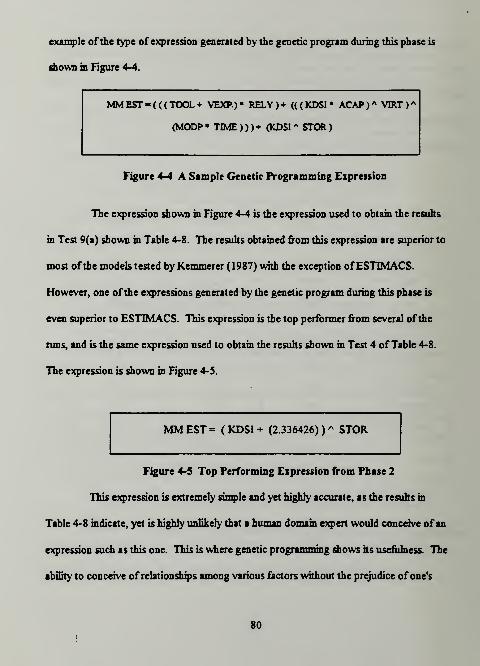
example ofthe type of expression generated by the genetic program during this phase is
shown m Figure 4-4.
MMEST-(((TOOL+ VEXR)» RELY) + (((KDSI» ACAP) A VTRT)
(MODP» TIME)))+ (KDSI A STOR)
Figure 4-4 A Sample Genetic Programming Expression
The expression shown in Figure 4-4 is the expression used to obtain the results
in Test 9(a) shown in Table 4-8. The results obtained from this expression are superior to
most ofthe models tested by Kemmerer (1987) with the exception ofESTIMACS.
However, one ofthe expressions generated by the genetic program during this phase is
even superior to ESTIMACS. This expression is the top performer from several ofthe
runs, and is the same expression used to obtain the results shown in Test 4 ofTable 4-8.
The expression is shown in Figure 4-5.
MM EST = ( KDSI + (2.336426)
)
A STOR
Figure 4-5 Top Performing Expression from Phase 2
This expression is extremely simple and yet highly accurate, as the results in
Table 4-8 indicate, yet is highly unlikely that a human domain expert would conceive ofan
expression such as this one. This is where genetic programming shows its usefulness. The
ability to conceive of relationships among various factors without the prejudice ofone's
80

own knowledge is what allows the genetic program to succeed in its task. The results
from this phase of experiments indicate that genetic programming is an extremely usesful
technique for generating cost-estimation models and should be considered as a leading
candidate for use as a cost-estimation model generator.
The comparison ofthe a sample ofthe results of genetic programming with
those obtained by Kemmerer in his study shows that genetic programming is capable of
generating a model that is superior to any ofthese popular cost-estimation models. In
fact, upon examining the best models from each generation of all ofthe runs during this
phase showed that during the 20 generation cycle for each run, the genetic program rarely
generated a program with over 400% error. This means that at almost any time during
any run, the genetic program was generating expressions that were superior to both SLIM
and Intermediate COCOMO.
3. Genetic Program Structural Analysis
The analysis ofthe structures generated by the genetic program is a very
complex topic and is currently being studied by a variety ofresearchers worldwide.
Although researchers are of different opinions about the significance ofthe structures that
genetic programming produces, there are some basic characteristics that can be observed.
Analyzing the results of a genetic programming run shows that the genetic
programming paradigm can be very inventive. As an example, when Koza (1992, pg. 242)
first developed his LISP genetic programming software, the capability to generate
constant terms was not included. During an early run involving the discovery of
81

trigonometric identities he observed a peculiar term in the resulting LISP S-expression.
This term is shown in Figure 4-5.
2 - Sin(Sin(Sin(Sm(Sin(Sm(Sin(Sin(l))*Sin(Sin(l)))))))))
Figure 4-5 Genetic Programming Derived Constant
This term evaluates to 1.57, which is very close to the value of Pi divided by
two, a constant that is needed often in trigonometric problems. The discovery ofthis type
ofinventive behavior by the genetic program led Koza to modify the software to allow for
the creation ofrandom constants. Koza (1992, pg. 185) also observed a tendency for the
genetic program to take useful subtrees and repetitively use them to perform functions that
the genetic program found useful.
The structures derived by the genetic program for the second phase in these
experiments varied widely in their size and composition, although the use ofparsimony
and a reduced maximum tree depth tended to yield shorter structures that performed
better across project domains. Examples ofsome ofthe structures derived by the genetic
program for cost-estimation are shown in Figure 4-6.
Examining the structures in Figure 4-6, it is apparent that the genetic program
does not find all ofthe cost drivers useful. While KDSI, MODP, STOR, and TIME
appear with some regularity, other drivers such as TURN and SCED are not used at alL
This is where genetic programming can be unsettling to a user. While the user can give
copious amounts of data to the genetic program, there is no certainty that all of it will be
82

Test 2 Generation 6
MMEST = ((AAF A PCAP) + LEXP) + (((CPLX+ ((((1.615063)* KDSI) *
((DATA* TIME)* TOOL))+ ((KDSI A TIME) A PCAP))) A VIRT) - VIRT)
Validation Fitness= 109.51
Test 3 Generation 6
MM EST = KDSI * (AEXP + TIME)
Validation Fitness= 130.77
Test 9 Generation 6
MM EST - (TOOL + ((KDSI A (MODP • TIME)) + (KDSI A STOR))) * VIRT
Validation Fitness= 144.16
Test 9 Generation 10
MM EST = (((TOOL + VEXP) * RELY)+ (((KDSI* ACAP) A VIRT) A (MODP
TIME))) + (KDSI A STOR)
Validation Fitness= 1 12.01
Figure 4-6 Genetic Programming Derived Structures
used. The user has to be prepared to deal with structures that have no resemblence to
relationships that the user believes to exist within the domain. This factor may be a barrier
to acceptance for some managers, but ifthe models derived are statistically significant in
both accuracy and correlation they are hard to dismiss.
83

V. CONCLUSIONS AND RECOMMENDATIONS
A. CONCLUSIONS
The major objective ofthis thesis was to examine the effectiveness ofthree machine
learning techniques as applied to the field of software cost estimation. The driving factor
behind the investigation ofmachine learning in the cost estimation field is that current
software cost estimation models are both inaccurate and not very adaptable across
development domains. These are critical areas ofweakness since the Department of
Defense is the largest single software consumer in the world, and it develops software for
a wide variety of domains. Therefore, it is necessary that a software cost estimation
model be both accurate and easily adaptable in order to be considered successful The
premise ofthis research was that there probably were relationships among the various
software project factors that the current models did not capture and that a machine
learning approach, where the models are derived directly from the data, may prove
superior in both performance and adaptability.
The three machine learning techniques studied in this thesis have all proven through
the experiments conducted to have great usefulness in the area of software cost
estimation. Each technique studied also brings to this field certain particular capabilities.
Neural networks showed a strong capability to capture and learn the project data, and
make estimates ofreasonable accuracy that exhibited a high correlation with the project
actuals. When tested with data from outside the domain in which the networks were
84

developed, the neural networks showed a strong capability to generalize on the data that
was presented to them and make estimates that were superior to those of other
well-known models. This capability to make estimates across domains is critical when
seeking estimates on new projects with different development environments. Given the
limited amount of data that was available for testing the networks, they performed
surprisingly well. Neural networks also have an advantage in that they are relatively easy
to set up and train, and are certainly within the capabilities ofmost management personnel.
They also have the advantage ofbeing self-calibrating, as long as the network is
maintained by continually retraining with data from newly completed projects. While not
as accurate as some ofthe algorithmic models, neural networks are certainly worthy of
consideration, especially since they have the ability to deal with non-numeric, or symbolic,
data. The best use of a neural network within an organization is probably at the earliest
stages where estimates that can at least capture the likely magnitude of a project are the
most useful
The genetic algorithm experiments showed that they were highly effective as a tool
for model optimization and calibration. Given no more than a fitness function, a table of
literal values describing the projects, and a small amount ofdomain knowledge in the guise
of constraints on the fitness function, the genetic algorithm was able to find a complete set
ofvalues for the cost drivers, coefficients, and exponents in the Intermediate COCOMO
model. The resulting model values were shown to provide estimates that had a high
degree ofaccuracy and correlation for projects developed within the same domain, but
85

their performance was not as good when applied to projects outside ofthe domain in
which they were trained. Still, the genetic algorithm proved to be effective as a tool for
model calibration and it is easy to apply. The user has only to supply a fitness function
that includes the fitness measure, the model function and whatever constraints the user
feels necessary for the particular domain. The power of evolution handles the search for
an optimal solution. Additionally, the genetic algorithm is highly extensible due to the
ability ofthe chromosome structure to be modified to reflect additional characteristics of
the domain. The genetic algorithm is likely to be ofthe greatest use in a situation where an
organization feels they have a model for how their development process functions but they
need a method for calibrating the model to the data at hand. The genetic algorithm is very
capable in this situation.
In the third set of experiments the very new technique ofgenetic programming was
used as a means for model discovery. In this case, the only inputs provided were the
fitness measure, the project data, and a set of functions that were allowed to operate on
the data. Upon initializing the population with a random set ofprograms, the process of
evolution then generated models ofgreater and greater fitness as the genetic program
evolved through succeeding generations. The models resulting from this technique were
both highly accurate and strongly correlated. These results indicate that genetic
programming shows great usefulness as an exciting new approach to the cost estimation
problem and has probably the broadest range ofuses of any ofthe techniques studied in
this thesis.
86

In all instances, each ofthe methods examined in this thesis was capable ofgenerating
models that were competitive in both accuracy and correlation with other established cost
estimation models. In one case, the machine generated model outperformed all ofthe
more well-known and established models. This level ofperformance exhibited by machine
generated models indicates that they should be given serious consideration by those
involved in the software development field, as they offer several advantages. First, they
directly reflect the data they are trained with, which automatically gives them an advantage
over a models that may have been developed outside ofthe domain in which it is being
applied. Second, they are highly extensible, meaning that any additional knowledge that
becomes available regarding the software development process can easily be incorporated
in these models. This provides an advantage over the more traditional models in that a
machine generated model is easily tailored to the data available. These advantages,
coupled with the performance levels noted in the experiments conducted in this study
indicate that machine learning is an effective and useful technique for the field of software
cost estimation.
B. RECOMMENDATIONS FOR FURTHER RESEARCH
There are several areas that are candidates for further research based on this study.
First, additional experiments can be conducted to extend the level ofknowledge regarding
how each ofthe techniques should be applied to achieve the greatest effectiveness.
Secondly, research can be conducted into coupling these machine learning techniques
together in order to create a suite oftools that may be able to provide a superior level of
87

performance. As as example, one could build an expert system front end that could query
a user about project characteristics in order to populate a data base. This expert system
front end could then be coupled to a neural network that could provide general estimates,
or it could be coupled to the genetic program, which could generate candidate models. It
may also be possible to have a neural network monitor the results of the models the
genetic program develops, and make a selection as to which model is best for a particular
situation based on the user's inputs the expert-system front-end. Finally, a similar set of
experiments to those conducted in this study could be performed using data from a variety
ofdomains for training. This may prove insightful, since a certain amount of
meta-knowledge about the data would have to be apparent in any models developed using
these techniques.
88

APPENDIX A
COCOMO DATA SET (Boehm, 1981, pg. 496)
pr
•
J
•
c
1
MMACTUAL
TOTKDSI
AAF
RELY
DATA
CPLX
T
ME
S
TOR
V
RT
TDRM
ACAP
AEXP
PCAP
VEXP
LEXP
MODP
TOOL
S
cED
MODE
1 2.040 113 1 088 1 16 07 1 106 1.15 107 1.19 1 13 1 17 11 1 124 1.1 104 E
2 1.600 293 0.85 088 1 16 0.85 1 1.06 1 107 1 91 1 09 0.95 1.1 1 1 E
3 243 132 1 1 1.16 0.85 1 1 087 094 86 82 086 09 0.95 91 0.91 1 SD
4 240 60 0.76 0.75 1.16 0.7 1 1 087 1 1 19 0.91 1 42 1 0.95 1.24 1 1.04 ORG
5 33 16 1 0.88 0.94 1 1 1 087 1 1 1 086 09 0.95 1.24 1 1 ORG
6 43 4 1 0.75 1 0.85 1 1.21 1 1 1.46 1 1 42 09 0.95 1.24 1.1 1 ORG
7 8 6.9 1 0.75 1 1 1 1 087 087 1 1 1 0.9 0.95 91 0.91 1 ORG
8 1.075 22 1 1.15 0.94 1.3 166 156 13 1 0.71 0.91 1 1.21 1.14 1.1 1.1 1.08 E
9 423 30 1 1.15 0.94 1.3 1.3 1.21 1 15 1 0.86 1 086 1.1 1.07 91 1 1 E
10 321 29 063 1.4 0.94 1.3 111 1 56 1 1.07 0.86 082 086 09 1 1 1 1 E
11 218 32 0.63 1.4 094 1.3 1.11 1 56 1 1.07 0.86 0.82 086 0.9 1 1 1 1 E
12 201 37 1 1.15 0.94 1.3 1.11 1.06 1 1 0.86 0.82 86 1 0.95 091 1 1.08 E
13 79 25 0.96 1.15 0.94 1.3 1.11 106 1.15 1 071 1 0.7 11 1 82 1 1 E
14 73 3 1 1.15 0.94 1.65 1.3 1.56 1 15 1 0.86 1 0.7 1.1 1.07 1.1 1.24 1.23 SD
15 61 3.9 1 1.4 0.94 1.3 1.3 106 1 15 87 0.86 1 13 086 1.21 1 14 0.91 1 1.23 E
16 40 6.1 0.6 1.4 1 1.3 1.3 1.56 1 0.87 0.86 1 086 1 1 1 1 1 E
17 9 3.6 0.53 1.4 1 1.3 1.3 1.56 1 087 0.86 0.82 0.86 1 1 1 1 1 E
18 11.400 320 1 1.15 1.16 1.15 1.3 1.21 1 107 0.86 1 1 1 1 1.24 1.1 108 E
19 6.600 1.150 0.84 1.15 1.08 1 111 1.21 087 094 0.71 0.91 1 1 1 091 0.91 1 E
20 6.400 299 0.96 1.4 1.08 1.3 1.11 1.21 1.15 1.07 0.71 0.82 108 1.1 1.07 1.24 1 1.08 SD
21 2.455 252 1 1 1.16 1.15 1.06 1.14 0.87 0.87 0.86 1 1 1 1 0.91 0.91 1 E
22 724 118 0.92 1.15 1 1 1.27 1.06 1 1 0.86 0.82 86 09 1 0.91 1 1.23 E
23 S39 77 0.98 1.15 1 1 108 1.06 1 1 0.86 0.82 0.86 0.9 1 1 1 1.23 E
24 453 90 1 0.88 1 085 1.06 106 1 0.87 1 1.29 1 1.1 0.95 0.82 0.83 1 SD
89
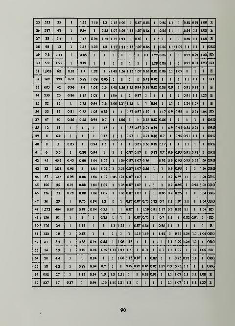
25 523 38 1 1.15 1.16 1.3 1 15 106 1 0.87 0.86 1 0.86 1.1 1 0.82 0.91 1.08 E
26 387 48 1 0.94 1 0.85 1.07 1 06 1 15 1.07 0.86 1 0.86 1.1 1 0.91 1.1 1.08 E
27 88 9.4 1 1.15 0.94 1.15 1.35 1.21 1 0.87 1 1 1 1 1 0.82 1.1 1.08 E
28 98 13 1 1.15 1.08 1.3 1.11 1.21 1.15 1.07 0.86 1 0.86 1.1 1.07 1.1 1.1 1 ORG
29 7J 2.14 1 0.88 1 1 1 1 1 1 1.1 1.29 0.86 1 1 0.91 0.91 1.23 SD
30 5.9 1.98 1 0.88 1 1 1 1 1 1 1 1.29 0.86 1 1 0.91 0.91 1.23 SD
31 1.063 62 0.81 14 1.08 1 148 1 56 1 15 1.07 0.86 0.82 0.86 11 1.07 1 1 1 E
32 702 390 0.67 0.88 1.08 0.85 1 1 1 1 0.71 082 1 1 1 1.1 1.1 1 SD
33 605 42 0.96 1.4 1.08 1.3 1 48 1.56 1.15 0.94 0.86 082 0.86 09 1 0.91 0.91 1 E
34 230 23 0.96 1.15 1.08 1 1.06 1 1 0.87 1 1 1 1 1 0.91 1.1 1.23 E
35 82 13 1 0.75 0.94 1.3 106 1.21 1.15 1 1 091 1 11 1 1.24 1.24 1 E
36 55 15 0.81 0.88 1.08 0.85 1 1 087 0.87 1.19 1 1.17 09 0.95 1 0.91 1.04 SD
37 47 60 0.56 088 0.94 0.7 1 1 06 1 1 0.86 0.82 0.86 1 1 1 1 1 ORG
38 12 15 1 1 1 1.15 1 1 087 0.87 071 091 1 09 0.95 082 0.91 1 ORG
39 8 6.2 1 1 1 1.15 1 1 87 1 0.71 82 0.7 1 0.95 0.91 1.1 1 ORG
40 8 3 0.83 1 0.94 1.3 1 1 1 0.87 0.86 082 1.17 1 1 1.1 1 1 ORG
4] 6 5.3 1 0.88 0.94 1 1 1 0.87 0.87 1 82 0.7 0.9 0.95 0.91 0.91 1 ORG
42 45 45.5 0.43 0.88 1.04 1.07 1 1 06 0.87 1.07 0.86 1 0.93 09 0.95 0.95 0.95 1.04 ORG
43 83 28.6 0.98 1 1.04 1.07 1 1.21 0.87 1.07 0.86 1 1 09 0.95 1 1 1.04 ORG
44 87 30.6 0.98 0.88 1.04 1.07 1 06 1.21 0.87 1.07 1 1 1 0.9 0.95 1.1 1 1.04 ORG
45 106 35 0.91 0.88 1.04 1.07 1 106 87 1.07 1 1 1 0.9 0.95 1 0.95 1.04 ORG
46 126 73 0.78 0.88 1.04 1.07 1 1.06 0.87 1.07 1 1 0.86 0.9 0.95 1 1 1.04 ORG
47 36 23 1 0.75 0.94 1.3 1 1 0.87 0.87 0.71 0.82 0.7 1.1 1.07 1.1 1 1.04 ORG
48 1.272 464 0.67 0.88 094 0.85 1 1 087 1 1.19 091 1.17 0.9 095 1.1 1 1.04 SD
49 156 91 1 1 0.85 1 1 1 0.87 0.71 1 0.7 11 1 0.82 0.91 1 SD
50 176 24 1.15 1 1 1.3 1.21 1 0.87 0.86 1 0.86 11 1 1 1 1 E
51 122 10 0.88 1 1 1 1 1 1.15 1.19 1 1.42 1 0.95 1.24 1.1 1.04 ORG
52 41 8.2 0.88 0.94 0.85 1 106 1.15 1 1 1 1 1.1 1.07 1.24 1.1 1 ORG
53 14 5.3 088 0.94 1.15 111 1.21 1.3 1 0.71 1 0.7 1.1 1.07 1 1.1 1.08 SD
54 20 4.4 1 0.94 1 1 1.06 1 15 0.87 1 0.82 1 1 0.95 0.91 1.1 ] ORG
55 18 6.3 0.88 0.94 0.7 1 1 087 0.87 0.86 0.82 1.17 0.9 0.95 1.1 1 1 ORG
56 958 27 1.15 0.94 U 1.3 1.21 1 1 0.86 091 1 11 1.07 1.1 1.1 1.08 E
57 237 17 0.87 1 0.94 1.15 111 1.21 1.3 1 1 1 1 1.1 1.07 1.1 1.1 1.23 E
90

58 130 25 1 1.4 0.94 1.3 1 66 1.21 1 1 0.71 0.82 07 0.9 0.95 0.91 1 1 £
59 70 23 0.9 1 0.94 1.15 1.06 1.06 1 0.87 1 1 1 1 1 091 1 1 ORG
60 57 6.7 1 1.15 0.94 1.3 1.11 1.06 1 1 0.86 113 086 1.1 1.07 1.1 1.1 1.08 ORG
61 50 28 1 1 0.94 1.15 1 1 0.87 0.87 086 1 086 0.9 1 0.82 1 1 ORG
62 38 9.1 1 088 0.94 1.3 1.11 1.21 1.15 1 078 0.82 0.7 1.21 1.14 0.91 1.24 1 SD
63 15 10 1 1 0.94 1.15 1 1 1 087 0.71 0.82 086 1 1 0.82 1 1 E
91
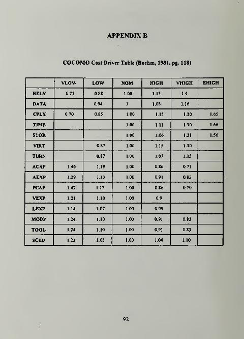
APPENDIX B
COCOMO Cost Driver Table (Boehm, 1981, pg. 118)
VLOW LOW NOM HIGH VH3GH EHIGH
RELY 0.75 0.88 1.00 1.15 1.4
DATA 0.94 1 1.08 1.16
CPLX 0.70 0.85 1.00 1.15 1.30 1.65
TIME 1.00 1.11 1.30 1.66
STOR 1.00 1.06 1.21 1.56
VIRT 0.87 1.00 1.15 1.30
TURN 0.87 1.00 1.07 1.15
ACAP 1.46 1.19 1.00 0.86 0.71
AEXP 1.29 1.13 1.00 0.91 0.82
PCAP 1.42 1.17 1.00 0.86 0.70
VEXP 1.21 1.10 1.00 0.9
LEXP 1.14 1.07 1.00 0.95
MODP 1.24 1.10 1.00 0.91 0.82
TOOL 1.24 1.10 1.00 0.91 0.83
SCED 1.23 1.08 1.00 1.04 1.10
92

APPENDIX C
Kemmerer Data Set
pr
•
1
t
c
t
MM
ACT
KDS
AAF
RELY
DATA
CPLX
T
ME
STOR
VI
RT
TURN
ACAP
AEXP
PCAP
VEXP
LEXP
MODP
TOOL
S
cED
MODE
1 287 253 6 1 1.15 108 1.15 1 106 087 1 086 1.13 0.86 1 1 0.82 0.91 1.02 SD
2 82.5 40.5 1 1 1 1 1 0.87 1 1 1.07 0.86 1 1 1 1 1 SD
3 1.107.
31
450 1 1.16 1 1.3 1.21 0.87 1 0.86 1.13 1 1 1.03 0.91 1 1 E
4 86.9 2144 1 1.08 0.92 1 1 0.87 0.93 0.8 089 0.85 0.97 0.95 1 1 1.02 SD
5 336.3 449.9 1 0.94 1 1 1 0.93 0.87 0.78 1 13 0.93 1.1 1.03 1 0.91 1.07 ORG
6 84 50 1 1.16 1 1.11 1.06 1 87 086 1 13 0.86 0.95 0.97 0.91 1 1.23 E
7 23.2 43 1 1.16 1 111 106 1 0.87 0.86 1.13 0.7 095 1.07 0.91 1 1.23 E
8 130.3 167 1 1.15 1.16 1 1 1 1 0.93 1 0.95 1 0.95 0.97 1 1 1.16 SD
9 116 289 1 1.16 1.15 111 1.06 087 0.87 1 1.13 1.06 1.1 1 1 1 1.08 E
10 72 39 1 1.16 1 1.11 1 0.93 1.03 0.71 1 0.7 1.1 1.14 1.05 1 1.23 SD
11 258.7 254.2 1 1.16 1 1 1 1 1 1 0.86 1.13 086 1 1 0.86 1 1.23 SD
ia 230.7 1286 1 1.16 1 1 1 087 0.87 0.86 1.07 0.86 1 1.03 1.1 0.95 1.08 SD
13 157 161.4 1 1.16 1 1.06 1 0.87 0.87 1.19 1 0.78 1.21 0.97 11 1 1.08 SD
14 246.9 164.8 1 1.16 1 1 1 0.87 0.87 0.86 1.21 0.93 11 1.1 0.95 0.91 1.04 ORG
15 69.9 60.2 1 1 1 1 1 1 0.87 0.71 0.91 086 1.1 1.03 0.91 0.91 1 SD
•AAI value.•sun given by Ken
93

APPENDIX D
COCOMO TRAINING AND TESTING DATA SETS
TRAINING DATA SETpr
o
J
•
c
t
MMACTUAL
TOTKDSI
AAF
RELY
DATA
cpLX
TI
ME
STOR
VI
RT
TURN
ACAP
AEXP
PCAP
VEXP
LEXP
MODP
TOOL
ScED
MODE
1 2,040 113 1 0.88 1.16 0.7 1 1.06 1.15 1.07 1.19 1.13 1.17 1.1 1 1.24 1.1 1.04 E
3 243 132 1 1 1.16 0.85 1 1 0.87 0.94 0.86 0.82 0.86 0.9 0.95 091 0.91 1 SD
4 240 60 0.76 0.75 1.16 0.7 1 1 0.87 1 1.19 0.91 1.42 1 0.95 1.24 1 1.04 ORG
5 33 16 1 0.88 0.94 1 •1 1 0.87 1 1 1 0.86 0.9 0.95 1.24 1 1 ORG
9 423 30 1 1.15 0.94 1.3 1.3 1.21 1.15 1 0.86 1 0.86 1.1 1.07 0.91 1 1 E
10 321 29 0.63 1.4 0.94 1.3 1.11 1.56 1 1.07 0.86 0.82 0.86 0.9 1 1 1 1 E
11 218 32 0.63 1.4 0.94 1.3 1.11 1.56 1 1.07 0.86 0.82 0.86 0.9 1 1 1 1 E
16 40 6.1 0.6 14 1 1.3 1.3 1.56 1 0.87 0.86 1 0.86 1 1 1 1 1 E
20 6.400 299 0.96 1.4 1.08 1.3 1.11 1.21 1.15 1.07 0.71 0.82 1.08 1.1 1.07 1.24 1 1.08 SD
21 2.455 252 1 1 1.16 1.15 1.06 1.14 0.87 0.87 0.86 1 1 1 1 0.91 0.91 1 E
22 724 118 0.92 1.15 1 1 1.27 1.06 1 1 0.86 0.82 0.86 0.9 1 0.91 1 1.23 E
23 539 77 0.98 1.15 1 1 1.08 1.06 1 1 0.86 0.82 0.86 0.9 1 1 1 1.23 E
24 453 90 1 0.88 1 0.85 1.06 1.06 1 0.87 1 1.29 1 1.1 0.95 0.82 0.83 1 SD
25 523 38 1 1.15 1.16 1.3 1.15 1.06 1 0.87 086 1 0.86 1.1 1 0.82 0.91 1.08 E
26 387 48 1 0.94 1 0.85 1.07 1.06 1.15 1.07 0.86 1 0.86 1.1 1 0.91 1.1 1.08 E
28 98 13 1 1.15 1.08 1.3 1.11 1.21 1.15 1.07 0.86 1 0.86 1.1 1.07 1.1 1.1 1 ORG
31 1.063 62 0.81 1.4 1.08 1 1.48 1.56 1.15 1.07 0.86 0.82 0.86 1.1 1.07 1 1 1 E
32 702 390 0.67 0.88 1.08 0.85 1 1 1 1 0.71 0.82 1 1 1 1.1 1.1 1 SD
33 605 42 0.96 14 1.08 1.3 1.48 1.56 1.15 094 0.86 0.82 0.86 0.9 1 0.91 0.91 1 E
34 230 23 0.96 1.15 1.08 1 1.06 1 1 0.87 1 1 1 1 1 0.91 1.1 1.23 E
35 82 13 1 0.75 0.94 1.3 1.06 1.21 1.15 1 1 0.91 1 1.1 1 1.24 1.24 1 E
36 55 15 0.81 0.88 1.08 0.85 1 1 0.87 0.87 1.19 1 1.17 0.9 0.95 1 0.91 1.04 SD
94

40 8 3 0.83 1 094 1.3 1 1 1 0.87 0.86 0.82 1.17 1 1 1.1 1 1 ORG
41 6 5.3 1 0.88 0.94 1 1 1 0.87 0.87 1 0.82 0.7 0.9 0.95 0.91 0.91 1 ORG
42 45 45.5 0.43 0.88 1.04 1.07 1 1.06 087 1.07 0.86 1 0.93 0.9 0.95 0.95 0.95 1.04 ORG
43 83 28.6 0.98 1 1.04 1.07 1 1.21 0.87 1.07 0.86 1 1 0.9 0.95 1 1 1.04 ORG
44 87 30.6 0.98 0.88 1.04 1.07 1.06 1.21 0.87 1.07 1 1 1 0.9 0.95 1.1 1 1.04 ORG
45 106 35 0.91 0.88 1.04 1.07 1 1.06 0.87 1.07 1 1 1 0.9 0.95 1 0.95 1.04 ORG
46 126 73 0.78 0.88 1.04 1.07 1 I 06 0.87 1.07 1 1 0.86 0.9 0.95 1 1 1.04 ORG
47 36 23 1 0.75 094 1J 1 1 0.87 0.87 0.71 0.82 0.7 1.1 1.07 1.1 1 1.04 ORG
48 1.272 464 0.67 0.88 0.94 0.85 1 1 0.87 1 1.19 0.91 1.17 0.9 0.95 1.1 1 1.04 SD
49 1S6 91 1 1 1 0.85 1 1 1 0.87 0.71 1 0.7 1.1 1 0.82 0.91 1 SD
50 176 24 1 1.15 1 1 1.3 1.21 1 0.87 0.86 1 0.86 1.1 1 1 1 1 E
51 122 10 1 0.88 1 1 1 1 1 1.15 1.19 1 1.42 1 0.95 1.24 1.1 1.04 ORG
53 14 5.3 1 0.88 0.94 1.15 1.11 1.21 1.3 1 0.71 1 0.7 1.1 1.07 1 1.1 1.08 SD
54 20 4.4 1 1 094 1 1 1.06 1.15 0.87 1 082 1 1 0.95 0.91 1.1 1 ORG
55 18 6.3 1 0.88 094 0.7 1 1 0.87 0.87 0.86 0.82 1.17 0.9 0.95 1.1 1 1 ORG
56 958 27 1 1.15 0.94 1.3 1.3 1.21 1 1 0.86 0.91 1 1.1 1.07 1.1 1.1 1.08 E
57 237 17 0.87 1 0.94 1.15 111 1.21 1.3 1 1 1 1 1.1 1.07 1.1 1.1 1.23 E
58 130 25 1 1.4 0.94 1.3 166 1.21 1 1 0.71 0.82 0.7 0.9 0.95 0.91 1 1 E
62 38 9.1 1 0.88 0.94 1.3 1.11 1.21 1.15 1 078 0.82 0.7 1.21 1 14 0.91 1.24 1 SD
63 15 10 1 1 0.94 1.15 1 1 1 0.87 071 0.82 0.86 1 1 0.82 1 1 E
95

COCOMO TESTING DATA SET
pr
•
J
•
c
t
MMACTUAL
TOTKDSI
AAF
RELY
DATA
CPLX
T
ME
STOR
V
RT
TVRN
ACAP
AEXP
PCAP
VEXP
LEXP
MODP
TOOL
ScED
MODE
2 1.600 293 0.85 0.88 1.16 0.85 1 1.06 1 1.07 1 0.91 1 0.9 0.95 1.1 1 1 E
6 43 4 1 0.75 1 0.85 1 1.21 1 1 146 1 142 0.9 0.95 1.24 1.1 1 ORG
7 8 6.9 1 0.75 1 1 1 1 0.87 0.87 1 1 1 0.9 0.95 0.91 0.91 1 ORG
8 1,075 22 1 1.15 0.94 1.3 1.66 1.56 13 1 0.71 0.91 1 1.21 1.14 1.1 1.1 1.08 E
12 201 37 1 1.15 0.94 1.3 1.11 1.06 1 1 0.86 0.82 0.86 1 0.95 0.91 1 1.08 E
13 79 25 0.96 1.15 0.94 1.3 1.11 1.06 1.15 1 0.71 1 0.7 1.1 1 0.82 1 1 E
14 73 3 1 1.15 0.94 1.65 1.3 1.56 1.15 1 0.86 1 0.7 1.1 1.07 1.1 1.24 1.23 SD
15 61 3.9 1 1.4 0.94 1.3 1.3 1.06 1.15 0.87 0.86 1.13 0.86 1.21 1.14 0.91 1 1.23 E
17 9 3.6 0.53 14 1 1.3 1.3 1.56 1 0.87 0.86 0.82 0.86 1 1 1 1 1 E
18 11.400 320 1 1.15 1.16 1.15 1.3 1.21 1 1.07 086 1 1 1 1 1.24 1.1 108 E
19 6.600 1.150 084 1.15 1.08 1 1.11 1.21 0.87 0.94 0.71 0.91 1 1 1 0.91 0.91 1 E
27 88 9.4 1 1.15 094 1.15 1.35 1.21 1 0.87 1 1 1 1 1 0.82 1.1 1.08 E
29 7.3 214 1 0.88 1 1 1 1 1 1 1.1 1.29 0.86 1 1 0.91 0.91 1.23 SD
30 5.9 1.98 1 0.88 1 1 1 1 1 1 1 1.29 0.86 1 1 0.91 0.91 1.23 SD
37 47 60 0.56 0.88 0.94 0.7 1 1.06 1 1 0.86 0.82 0.86 1 1 1 1 1 ORG
38 12 15 1 1 1 1.15 1 1 0.87 0.87 0.71 0.91 1 0.9 0.95 0.82 0.91 1 ORG
39 8 6.2 1 1 1 1.15 1 1 0.87 1 071 0.82 0.7 1 0.95 0.91 1.1 1 ORG
52 41 8.2 1 088 0.94 0.85 1 1.06 1.15 1 1 1 1 1.1 1.07 1.24 1.1 1 ORG
59 70 23 0.9 1 0.94 1.15 1.06 1.06 1 0.87 1 1 1 1 1 0.91 1 1 ORG
60 57 6.7 1 1.15 0.94 1.3 1.11 1.06 1 1 0.86 1.13 0.86 1.1 1.07 1.1 1.1 1.08 ORG
61 50 28 1 1 0.94 1.15 1 1 0.87 0.87 0.86 1 0.86 0.9 1 0.82 1 1 ORG
96

APPENDIX E
BrainMaker Neural Network Definition Files (\DEF)
COCOMO Training/Kemmerer Testing Version
•ft********************************************************************
Network 5/8
input number 1 20
dictionary input LOG_KDSI AAF RELY DATA CPLX TIME STOR VIRT TURNACAP AEXP PCAP VEXP LEXP MODP TOOL SCED E SD ORGoutput number 1 1
dictionary output LOG_MMAChidden S 8
filename trainfacts c:\brain\test\cokealll.fct
filename runiacts c:\brain\test\kemmer.in
leamrate 0.9000 50 0.75 75 0.6000 90 0.5000
learnlayeT 1.0000 1.0000 1.0000
traintol 0.1000 0.04 0.8000 100
testtol 0.2000
random 5.0
maxruns459
function hidden 1 sigmoid 0.0000 1.0000 0.0000 1.00000
function hidden2 sigmoid 0.0000 1.0000 0.0000 1.00000
function output sigmoid 0.0000 1.0000 0.0000 1.00000
LOGJKDS AAF RELY DATA CPLX TIME STOR VIRT TURNACAP AEXP PCAP VEXP LEXP MODP TOOL SCED E SDORGLOG_MMAscale input minimum
0.29666 0.43 0.75 0.94 0.7 1 1 0.87 0.87 0.71 0.82 0.7 0.9
0.95 0.82 0.83 1000scale input maximum3.06069 1 1.4 1.16 1.65 1.66 1.56 1.3 1.15 1.46 1.29 1.42 1.21
1.14 1.24 1.24 1.23 1 1 1
scale output minimum
0.77085
scale output maximum4.0569
97

ft**********************************************************************
Network 8/9
***********************************************************************
input number 1 20
dictionary input LOGKDSI AAF RELY DATA CPLX TIME STOR VIRT TURNACAP AEXP PCAP VEXP LEXP MODP TOOL SCED E SD ORGoutput number 1 1
dictionary output LOG_MMAChidden 8 9
filename trainfacts c:\brain\test\cokeaIll.fct
filename runfacts c:\brain\test\kemmer.in
leamrate 0.9000 50 0.75 75 0.6000 90 0.5000
leamlayer 1.0000 1.0000 1.0000
traintol 0.1000 0.04 0.8000 100
testtol 0.2000
random 5.0
maxruns 430
function hidden 1 sigmoid 0.0000 1.0000 0.0000 1.00000
function hidden2 sigmoid 0.0000 1.0000 0.0000 1.00000
function output sigmoid 0.0000 1.0000 0.0000 1.00000
LOG_KDS AAF RELY DATA CPLX TIME STOR VIRT TURNACAP AEXP PCAP VEXP LEXP MODP TOOL SCED E SDORG
1 0.87 0.87 0.71 0.82 0.7 0.9
LOG_MMAscale input minimum0.29666 0.43 0.75 0.94 0.7
0.95 0.82 0.83 1 000scale input maximum3.06069 1 1.4 1.16 1.65
1.14 1.24 1.24 1.23 1 1 1
Scale Output minimum
0.77085
scale output maximum4.0569
.66 1.56 1.3 1.15 1.46 1.29 1.42 1.21
98
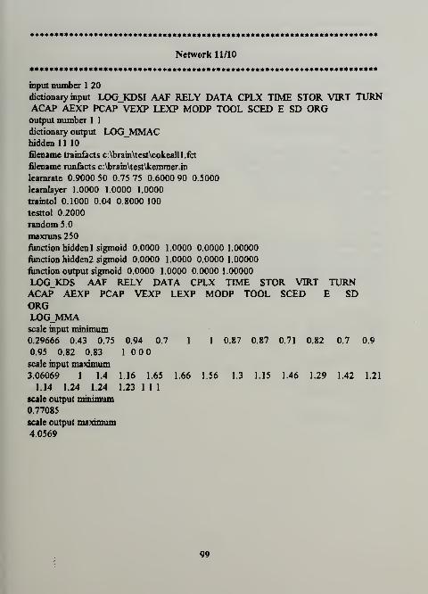
***********************************************************************
Network 11/10
***********************************************************************
input number 1 20
dictionary input LOGKDSI AAF RELY DATA CPLX TIME STOR VIRT TURNACAP AEXP PCAP VEXP LEXP MODP TOOL SCED E SD ORGoutput number 1 1
dictionary output LOG_MMAChidden 11 10
filename trainiacts c:\brain\test\cokealll.fct
filename runfacts c:\brain\test\kemmer.in
learnrate 0.9000 50 0.75 75 0.6000 90 0.5000
learnlayer 1.0000 1.0000 1.0000
traintol 0.1000 0.04 0.8000 100
testtol 0.2000
random 5.0
maxruns 250
function hidden 1 sigmoid 0.0000 1.0000 0.0000 1.00000
function hidden2 sigmoid 0.0000 1.0000 0.0000 1.00000
function output sigmoid 0.0000 1.0000 0.0000 1.00000
LOG_KDS AAF RELY DATA CPLX TIME STOR VIRT TURNACAP AEXP PCAP VEXP LEXP MODP TOOL SCED E SDORGLOG_MMAscale input minimum
0.29666 0.43 0.75 0.94 0.7 1 1 0.87 0.87 0.71 0.82 0.7 0.9
0.95 0.82 0.83 1000scale input maximum3.06069 1 1.4 1.16 1.65 1.66 1.56 1.3 1.15 1.46 1.29 1.42 1.21
1.14 1.24 1.24 1.23 1 1 1
scale output minimum
0.77085
scale output maximum4.0569
99

***********************************************************************
Network 16/19
***********************************************************************
input number 1 20
dictionary input LOGKDSI AAF RELY DATA CPLX TIME STOR VIRT TURNACAP AEXP PCAP VEXP LEXP MODP TOOL SCED E SD ORGoutput number 1 1
dictionary output LOG_MMAChidden 16 19
filename trainfacts c:\brain\test\cokealll.fct
filename runfacts c:\brain\test\kemmer.in
leamrate 0.9000 50 0.75 75 0.6000 90 0.5000
leamlayer 1.0000 1.0000 1.0000
traintol 0.1000 0.04 0.8000 100
testtol 0.2000
random 5.0
maxruns 304
function hidden 1 sigmoid 0.0000 1.0000 0.0000 1.00000
function hidden2 sigmoid 0.0000 1.0000 0.0000 1.00000
function output sigmoid 0.0000 1.0000 0.0000 1.00000
LOGKDS AAF RELY DATA CPLX TIME STOR VIRT TURNLEXP MODP TOOL SCED E SD
1 0.87 0.87 0.71 0.82 0.7 0.9
ACAP AEXP PCAP VEXPORGLOG_MMAscale input minimum0.29666 0.43 0.75 0.94 0.7
0.95 0.82 0.83 1 000scale input maximum3.06069 1 1.4 1.16 1.65
1.14 1.24 1.24 1.23 1 1 1
scale output minimum
0.77085
scale output maximum4.0569
.66 1.56 1.3 1.15 1.46 1.29 1.42 1.21
100
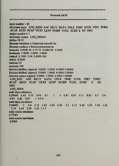
**********************************************************************
Network 18/15
***********************************************************************
input number 1 20
dictionary input LOG_KDSI AAF RELY DATA CPLX TIME STOR VIRT TURNACAP AEXP PCAP VEXP LEXP MODP TOOL SCED E SD ORGoutput number 1 1
dictionary output LOG_MMAChidden 18 IS
filename trainfacts c:\brain\test\cokealll.fct
filename runfacts c:\brain\test\kemmer.in
leamrate 0.9000 50 0.75 75 0.6000 90 0.5000
learnlayer 1.0000 1.0000 1.0000
traintol 0.1000 0.04 0.8000 100
testtol 0.2000
random 5.0
maxruns318
function hidden 1 sigmoid 0.0000 1.0000 0.0000 1.00000
function hidden2 sigmoid 0.0000 1.0000 0.0000 1.00000
function output sigmoid 0.0000 1.0000 0.0000 1.00000
LOGJCDS AAF RELY DATA CPLX TIME STOR VIRT TURNACAP AEXP PCAP VEXP LEXP MODP TOOL SCED E SDORG
1 0.87 0.87 0.71 0.82 0.7 0.9
LOG_MMAscale input minimum
0.29666 0.43 0.75 0.94 0.7
0.95 0.82 0.83 1 000scale input maximum3.06069 1 1.4 1.16 1.65
1.14 1.24 1.24 1.23 1 1 1
scale output minimum
0.77085
scale output maximum4.0569
1.66 1.56 1.3 1.15 1.46 1.29 1.42 1.21
101
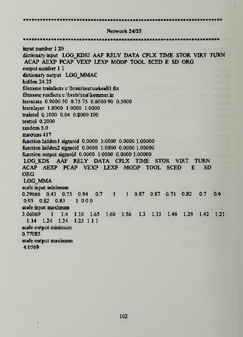
***********************************************************************
Network 24/25
**********************************************************************
input number 1 20
dictionary input LOGKDSI AAF RELY DATA CPLX TIME STOR VIRT TURNACAP AEXP PCAP VEXP LEXP MODP TOOL SCED E SD ORGoutput number 1 1
dictionary output LOG_MMAChidden 24 25
filename trainfacts c:\brain\test\cokealll.fct
filename runfacts c:\brain\test\kemmer.in
learnrate 0.9000 50 0.75 75 0.6000 90 0.5000
learnlayer 1.0000 1.0000 1.0000
traintol 0.1000 0.04 0.8000 100
testtol 0.2000
random 5.0
maxruns417
function hidden! sigmoid 0.0000 r.OOOO 0.0000 1.00000
function hidden2 sigmoid 0.0000 1.0000 0.0000 1.00000
function output sigmoid 0.0000 1.0000 0.0000 1.00000
LOGKDS AAF RELY DATA CPLX TIME STOR VIRT TURNACAP AEXP PCAP VEXP LEXP MODP TOOL SCED E SDORG
1 1 0.87 0.87 0.71 0.82 0.7 0.9
LOG_MMAscale input minimum0.29666 0.43 0.75 0.94 0.7
0.95 0.82 0.83 1 000scale input maximum3.06069 1 1.4 1.16 1.65
1.14 1.24 1.24 1.23 1 1 1
Scale Output minimum
0.77085
scale output maximum4.0569
.66 1.56 1.3 1.15 1.46 1.29 1.42 1.21
102

Brainmaker Neural Network Training and Testing Files
COCOMO Training and Kemmerer Testing Versions
**********************************************************************
COKEALL1.FCT**********************************************************************
frets
2.05307 1 0.88 1.16 0.7 1 1.06 1.15 1.07 1.19 1.13 1.17 1.1
1 1.24 1.1 1.04 [ E3.30963
2.46686 0.85 0.88 1.16 0.85 1 1.06 1 1.07 1 0.91 1 0.9
0.95 1.1 1 1 [ E3.20412
2.12057 1 1 1.16 0.85 1 1 0.87 0.94 0.86 0.82 0.86 0.9
0.95 0.91 0.91 1 [ SD2.3856
4
1.77815 0.76 0.75 1.16 0.7 1 1 0.87 1 1.19 0.91 1.42 1
0.95 1.24 1 1.04 [ ORG2.38021
1.20412 1 0.88 0.94 1 1 1 0.87 1 1 1 0.86 0.9
0.95 1.24 1 1 [ ORG1.51851
6
0.60206 1 0.75 1 0.85 1 1.21 1 1 1.46 1 1.42 0.9
0.95 1.24 1.1 1 [ ORG1.63346
0.83884 1 0.75 1111 0.87 0.87 1 1 1 0.9 0.95
0.91 0.91 1 [ ORG0.90309
8
1.34242 1 1.15 0.94 1.3 1.66 1.56 1.3 1 0.71 0.91 1 1.21
1.14 1.1 1.1 1.08 [ E3.0314
9
103
1.47712 1 1.15 0.94 1.3 1.3 1.21 1.15 1 0.86 1 0.86 1.1
1.07 0.91 1 1 [ E2.62634
10
1.46239 0.63 1.4 0.94 1.3 1.11 1.56 1 1.07 0.86 0.82 0.86 0.9
1 1 1 1 [ E2.5065
11
1.50515 0.63 1.4 0.94 1.3 1.11 1.56 1 1.07 0.86 0.82 0.86 0.9
1 1 1 1 [ E2.33845
12
1.5682 1 1.15 0.94 1.3 1.11 1.06 1 1 0.86 0.82 0.86 1
0.95 0.91 1 1.08 [ E2.30319
13
1.39794 0.96 1.15 0.94 1.3 1.11 1.06 1.15 1 0.71 1 0.7 1.1
1 0.82 1 1 [ E1.89762
14
0.47712 1 1.15 0.94 1.65 1.3 1.56 1.15 1 0.86 1 0.7 1.1
1.07 1.1 1.24 1.23 [ SD1.86332
15
0.59106 1 1.4 0.94 1.3 1.3 1.06 1.15 0.87 0.86 1.13 0.86 1.21
1.14 0.91 1 1.23 [ E1.78533
16
0.78533 0.6 1.4 1 1.3 1.3 1.56 1 0.87 0.86 1 0.86 1
1 1 1 1 [ E1.60206
17
0.5563 0.53 1.4 1 1.3 1.3 1.56 1 0.87 0.86 0.82 0.86 1
1 1 1 1 [ E0.95424
18
2.50515 1 1.15 1.16 1.15 1.3 1.21 1 1.07 0.86 1 1 1
1 1.24 1.1 1.08 [ E4.0569
19
3.06069 0.84 1.15 1.08 1 1.11 1.21 0.87 0.94 0.71 0.91 1 1
1 0.91 0.91 1 [ E3.81954
104

20
2.47567 0.96 1.4 1.08 1.3 1.11 1.21 1.15 1.07 0.71 0.82 1.08
1.1 1.07 1.24 1 1.08 [ SD3.80618
21
2.4014 1 1 1.16 1.15 1.06 1.14 0.87 0.87 0.86 1 1 1
1 0.91 0.91 1 [ E3.39005
22
2.07188 0.92 1.15 1 1 1.27 1.06 1 1 0.86 0.82 0.86 0.9
1 0.91 1 1.23 [ E2.85973
23
1.88649 0.98 1.15 1 1 1.08 1.06 1 1 0.86 0.82 0.86 0.9
1 1 1 1.23 [ E2.73158
24
1.95424 1 0.88 1 0.85 1.06 1.06 1 0.87 1 1.29 1 1.1
0.95 0.82 0.83 1 [ SD2.65609
25
1.57978 1 1.15 1.16 1.3 1.15 1.06 1 0.87 0.86 1 0.86 1.1
1 0.82 0.91 1.08 [ E2.7185
26
1.68124 1 0.94 1 0.85 1.07 1.06 1.15 1.07 0.86 1 0.86 1.1
1 0.91 1.1 1.08 [ E2.58771
27
0.97312 1 1.15 0.94 1.15 1.35 1.21 1 0.87 11111 0.82 1.1 1.08 [ E1.94448
28
1.11394 1 1.15 1.08 1.3 1.11 1.21 1.15 1.07 0.86 1 0.86 1.1
1.07 1.1 1.1 1 [ ORG1.99122
29
0.33041 1 0.88 1 1 1 1 1 1 1.1 1.29 0.86 1 1
0.91 0.91 1.23 [ SD0.86332
30
0.29666 1 0.88 1111111 1.29 0.86 1 1
0.91 0.91 1.23 [ SD
105

0.77085
31
1.79239 0.81 1.4 1.08 1 1.48 1.56 1.15 1.07 0.86 0.82 0.86 1.1
1.07 1 1 1 [ E3.02653
32
2.59106 0.67 0.88 1.08 0.85 1111 0.71 0.82 1 1
1 1.1 1.1 1 [ SD2.84633
33
1.62324 0.96 1.4 1.08 1.3 1.48 1.56 1.15 0.94 0.86 0.82 0.86
0.9 1 0.91 0.91 1 [ E2.78175
34
1.36172 0.96 1.15 1.08 1 1.06 1 1 0.87 111110.91 1.1 1.23 [ E
2.36172
35
1.11394 1 0.75 0.94 1.3 1.06 1.21 1.15 1 1 0.91 1 1.1
1 1.24 1.24 1 [ E1.91381
36
1.17609 0.81 0.88 1.08 0.85 1 1 0.87 0.87 1.19 1 1.17 0.9
0.95 1 0.91 1.04 [ SD1.74036
37
1.77815 0.56 0.88 0.94 0.7 1 1.06 1 1 0.86 0.82 0.86 1
1 1 1 1 [ ORG1.67209
38
1.17609 1 1 1 1.15 1 1 0.87 0.87 0.71 0.91 1 0.9
0.95 0.82 0.91 1 [ ORG1.07918
39
0.79239 1 1 1 1.15 1 1 0.87 1 0.71 0.82 0.7 1
0.95 0.91 1.1 1 [ ORG0.90309
40
0.47712 0.83 1 0.94 1.3 1 1 1 0.87 0.86 0.82 1.17 1
1 1.1 1 1 [ ORG0.90309
41
106
0.72427 1 0.88 0.94 1 1 1 0.87 0.87 1 0.82 0.7 0.9
0.95 0.91 0.91 1 [ ORG0.77815
42
1.65801 0.43 0.88 1.04 1.07 1 1.06 0.87 1.07 0.86 1 0.93 0.9
0.95 0.95 0.95 1.04 [ ORG1.65321
43
1.45636 0.98 1 1.04 1.07 1 1.21 0.87 1.07 0.86 1 1 0.9
0.95 1 1 1.04 [ ORG1.91907
44
1.48572 0.98 0.88 1.04 1.07 1.06 1.21 0.87 1.07 1 1 1 0.9
0.95 1.1 1 1.04 [ ORG1.93951
45
1.54406 0.91 0.88 1.04 1.07 1 1.06 0.87 1.07 1 1 1 0.9
0.95 1 0.95 1.04 [ ORG2.0253
46
1.86332 0.78 0.88 1.04 1.07 1 1.06 0.87 1.07 1 1 0.86 0.9
0.95 1 1 1.04 [ ORG2.10037
47
1.36172 1 0.75 0.94 1.3 1 1 0.87 0.87 0.71 0.82 0.7 1.1
1.07 1.1 1 1.04 [ ORG1.5563
48
2.66651 0.67 0.88 0.94 0.85 1 1 0.87 1 1.19 0.91 1.17 0.9
0.95 1.1 1 1.04 [ SD3.10448
49
1.95904 1 1 1 0.85 1 1 1 0.87 0.71 1 0.7 1.1 1
0.82 0.91 1 [ SD2.19312
50
1.38021 1 1.15 1 1 1.3 1.21 1 0.87 0.86 1 0.86 1.1
1 1 1 1 [ £2.24551
51
1 1 0.88 11111 1.15 1.19 1 1.42 1 0.95
1.24 1.1 1.04 [ ORG2.08636
107

52
0.91381 1 0.88 0.94 0.85 1 1.06 1.15 1 1 1 1 1.1
1.07 1.24 1.1 1 [ ORG1.61278
53
0.72427 1 0.88 0.94 1.15 1.11 1.21 1.3 1 0.71 1 0.7 1.1
1.07 1 1.1 1.08 [ SD1.14612
54
0.64345 1 1 0.94 1 1 1.06 1.15 0.87 1 0.82 1 1
0.95 0.91 1.1 1 [ ORG1.30103
55
0.79934 1 0.88 0.94 0.7 1 1 0.87 0.87 0.86 0.82 1.17 0.9
0.95 1.1 1 1 [ ORG1.25527
56
1.43136 1 1.15 0.94 1.3 1.3 1.21 1 1 0.86 0.91 1 1.1
1.07 1.1 1.1 1.08 [ E2.98136
57
1.23044 0.87 1 0.94 1.15 1.11 1.21 1.3 1 1 1 1 1.1
1.07 1.1 1.1 1.23 [ E2.37474
58
1.39794 1 1.4 0.94 1.3 1.66 1.21 1 1 0.71 0.82 0.7 0.9
0.95 0.91 1 1 [ E2.11394
59
1.36172 0.9 1 0.94 1.15 1.06 1.06 1 0.87 11111 0.91 1 1 [ ORG1.84509
60
0.82607 1 1.15 0.94 1.3 1.11 1.06 1 1 0.86 1.13 0.86 1.1
1.07 1.1 1.1 1.08 [ ORG1.75587
61
1.44715 1 1 0.94 1.15 1 1 0.87 0.87 0.86 1 0.86 0.9
1 0.82 1 1 [ ORG1.69897
62
0.95904 1 0.88 0.94 1.3 1.11 1.21 1.15 1 0.78 0.82 0.7 1.21
1.14 0.91 1.24 1 [ SD
108

1.57978
63
1 1 1 0.94 1.15 1 1 1 0.87 0.71 0.82 0.86 1 1
0.82 1 1 [ E1.17609
***********************************************************************
KEMMER.IN**********************************************************************
LOGKDS AAF RELY DATA CPLX TIME STOR VIRT TURNACAP AEXP PCAP VEXP LEXP MODP TOOL SCED SD EORGfacts run
1
2.40414
1 0.82
1.60745
1 1
3
2.65321
1.03 0.91
4
2.33122
0.95 1
5
2.65311
1.03 1
6
1.69897
0.97 0.91
7
1.63346
1.07 0.91
2.22271
0.97 1
9
2.46089
1.15 1.08 1.15 1 1.06 0.87 1 0.86 1.13 0.86 1
0.91 1.02 [ SD
11111 0.87 1 1 1.07 0.86 1 1
1 [ SD
1 1.16 1 1.3 1.21 0.87 1 0.86 1.13 1 1
1 1 [ E
1 1.08 0.92 1 1 0.87 0.93 0.8 0.89 0.85 0.97
1 1.02 [ SD
1 0.94 1 1 1 0.93 0.87 0.78 1.13 0.93 1.1
.91 1.07 [ ORG
1 1.16 1 1.11 1.06 1 0.87 0.86 1.13 0.86 0.95
1 1.23 [ E
1 1.16 1 1.11 1.06 1 0.87 0.86 1.13 0.7 0.95
1 1.23 [ E
1.15 1.16 1111 0.93 1 0.95
1 1.16 [ SD0.95
1 1.16 1.15 1.11 1.06 0.87 0.87 1 1.13 1.06 1.1
1 1 1 1.08 [ E10
109

1.59106 1 1 1.16 1 1.11 1 0.93 1.03 0.71 1 0.7 1.1
1.14 1.05 1 1.23 [ SD
2.40517 1 1.16 111111 0.86 1.13 0.86 1 1
0.86 1 1.23 [ SD12
2.10924 1 1 1.16 1 1 1 0.87 0.87 0.86 1.07 0.86 1
1.03 1.1 0.95 1.08 [ SD13
2.2079 1 1 1.16 1 1.06 1 0.87 0.87 1.19 1 0.78 1.21
0.97 1.1 1 1.08 [ SD14
2.21695 1 1 1.16 1 1 1 0.87 0.87 0.86 1.21 0.93 1.1
1.1 0.95 0.91 1.04 [ ORG15
1.77959 1111111 0.87 0.71 0.91 0.86 1.1
1.03 0.91 0.91 1 [ SD
110

APPENDIX F
***********************************************************************
Genetic Algorithm Fitness Function (fitc)
(Prior to instantiation of awk Wrapper)************************************************************************
tfnchide <math.h>
struct entry {
double effort;
double akdsi,
int U,i2,i3,i4,i5,i6,i7,i8,i9,il0,il I,il2,il3,il4,il5;
intie;
I;
Variable Declarations
struct entry tableD =
{
#include "table, c"
}
Dimension Table and Include
Fact File "table, c"
int size = (sizeoftable)/(sizeof( struct entry));
double fl(y)
register double *y;
{
double res;
double emm,
double exp;
static double x[96];
register int ij;
Dimension Array of 96 numbers for use
by the fitness function.
for(i = 0;i<90;i-H-){
x[i] = y[i]+200;
x[i]/= 400.0;
x[i]*=1.5;
x[i]+=.5;
}
Constrain cost driver size between 0.5
and 2.0. Constrain coefficients and
exponents between 0.0 and 4.0
111

for(i = 90;i<96;i++){x[i] = y[i] + 200;
x[i] /= 100;
}
for(res = 0, i= 0; i < 42; i+=6) {
if(! (x[i]< x[i+l])) res +=1000
ifl! (x[i]< x[i+2])) res +=1000
ifl! (x[i]< x[i+3])) res +=1000
ifl! (x[i]< x[i+4])) res +=1000
i%\ (x[i]< x[i+5])) res +=1000,
if(! (x[i+l]< x[i+2])) res +=1000
if(!(x[i+l]<x[i+3])) res +=1000
if(!(x[i+l]<x[i+4])) res +=1000
if(!(x[i+l]<x[i+5])) res +=1000
if(! (x[i+2]< x[i+3])) res +=1000
if^!(x[i+2]<x[i+4])) res +=1000
if(! (x[i+2]< x[i+5])) res +=1000
if(! (x[i+3]< x[i+4])) res +=1000
if(! (x[i+3]< x[i+5])) res +=1000
if(! (x[i+4]< x[i+5])) res+=1000
>
for(i=42;i<84;i+=6) {
if(! (x[i]> x[i+l])) res +=1000
if(! (x[i]> x[i+2])) res +=1000
if(! (x[i]> x[i+3])) res +=1000
if(! (x[i]> x[i+4])) res +=1000
if(! (x[i]> x[i+5])) res +=1000,
if{!(x[i+l]>x[i+2])) res +=1000
if(! (x[i+l]> x[i+3])) res +=1000
ifl!(x[i+l]>x[i+4])) res +=1000
if(! (x[i+l]> x[i+5])) res +=1000
if(! (x[i+2]> x[i+3])) res +=1000
if(! (x[i+2]> x[i+4])) res +=1000
ifl! (x[i+2]> x[i+5])) res +=1000
W (x[i+3]> x[i+4])) res +=1000
if(!(x[i+3]>x[i+5])) res +=1000
ifi^! (x[i+4]> x[i+5])) res+=1000
}
/*for<i=90;i<91;i++){
Penalty functions to force GA
to obey rules established by
Boehm for the first seven cost
drivers. Comment out if
unconstrained drivers are
desired.
Penalty functions to force GA
to obey rules established by
Boehm for drivers eight through
fourteen. Comment out if
unconstrained drivers are
desired.
112

if(! (x[i] < x[i+l] )) res +=1000;
W (x[i] < x[i+2] )) res +=1000;
if(! (x[i+l] < x[i+2])) res +=1000;
}
for(i=93;i<94;i++){
if(! (x[i] > x[i+l] )) res +=1000;
iSt\ (x[i] > x[i+2] )) res +=1000;
W (x[i+l] > x[i+2])) res +=1000;
}
*/
Penalty functions to force GA
to obey rules established by
Boehm for coefficients and
exponents. Comment out if
unconstrained drivers are
desired.
for(i = 0; i < size; i++) {
/* get product of cost drivers - goes from to 89.. treat as a 6x15 array*/
emm = x[table[i].il];
emm *= x[table[i].i2 + 6];
emm *= x[table[i].i3 + 6*2]
emm *= x[table[i].i4 + 6*3]
emm *= x[table[i].i5 + 6*4]
emm *= x[table[i].i6 + 6*5]
emm *= x[table[i].i7 + 6*6]
emm *= x[table[i].i8 + 6*7]
emm *= x[table[i].i9 + 6*8]
*=x[table[i].il0 + 6*9];Bold type is fitness measure
evaluation. Average relative error is
shown.
emm *= x[table[i].il 1 + 6*10]
emm *=x[table[i].il2 + 6*11]
emm *= x[table[i].il3 + 6*12]
emm *=x[table[i].il4 + 6*13]
emm *=x[table[i].il5 + 6*14]
emm *= x[table[i].ie+90]; /* coeff */
emm *= pow(table[i].akdsi, x[table[i].ie+93]); /* exponent */
res+=
»qrt(((tabIe[i].effort-emm)/(tabIe[i].effort))*((table(i].effort-emm)/(tablel!].effort)));
>
return res/size;
/* GAeval fl 10:200dg96 */
Bold underlined tvoc is GAucsd 1.4 declaration
for the chromosome. Translate as 10 bits per
number, range -200 to 200, 96 numbers total
113

***********************************************************************
Genetic Algorithm Input Data File: COCOMO Training and Testing Version
Format is {MM_Actual, Adjusted KDS1, 15 Cost Drivers, Mode
literal Driver Values Defined as:
= Very Lowl=Low2 = Nominal
3 = Mgh4 = VeryHigh
5 = Extra High
Mode Defined as:
= Embedded1 = Semidetached
2 = Organic
"Table.c"
***********************************************************************
{2040, 113, 1, 4, 0, 2, 3, 3, 3, 1, 1, 1, 1, 2, 0, 1, 3, 0},
{243, 132, 2, 4, 1, 2, 2, 1, 1, 3, 4, 3, 3, 3, 3, 3, 2, 1},
{240, 45.6, 0, 4, 0, 2, 2, 1, 2, 1, 3, 0, 2, 3, 0, 2, 3, 2),
{33, 16, 1, 1, 2, 2, 2, 1, 2, 2, 2, 3, 3, 3, 0, 2, 2, 2},
{423, 30, 3, 1, 4, 4, 4, 3, 2, 3, 2, 3, 1, 1, 3, 2, 2, 0},
{321, 18.27, 4, 1, 4, 3, 5, 2, 3, 3, 4, 3, 3, 2, 2, 2, 2, 0},
{218, 20.16, 4, 1, 4, 3, 5, 2, 3, 3, 4, 3, 3, 2, 2, 2, 2, 0},
{40, 3.66, 4, 2, 4, 4, 5, 2, 1, 3, 2, 3, 2, 2, 2, 2, 2, 0),
{6400, 287.04, 4, 3, 4, 3, 4, 3, 3, 4, 4, 2, 1, 1, 0, 2, 1, 1},
{2455, 252, 2, 4, 3, 3, 3, 1, 1, 3, 2, 2, 2, 2, 3, 3, 2, 0},
{724, 108.56, 3, 2, 2, 4, 3, 2, 2, 3, 4, 3, 3, 2, 3, 2, 0, 0},
{539, 75.46, 3, 2, 2, 3, 3, 2, 2, 3, 4, 3, 3, 2, 2, 2, 0, 0),
{453, 90, 1, 2, 1, 3, 3, 2, 1, 2, 0, 2, 1, 3, 4, 4, 2, 1},
{523, 38, 3, 4, 4, 3, 3, 2, 1, 3, 2, 3, 1, 2, 4, 3, 1, 0},
{387, 48, 1, 2, 1, 3, 3, 3, 3, 3, 2, 3, 1, 2, 3, 1, 1, 0},
{98, 13, 3, 3, 4, 3, 4, 3, 3, 3, 2, 3, 1, 1, 1, 1, 2, 2},
{1063, 50.22, 4, 3, 2, 4, 5, 3, 3, 3, 4, 3, 1, 1, 2, 2, 2, 0},
{702, 261.3, 1, 3, 1, 2, 2, 2, 2, 4, 4, 2, 2, 2, 1, 1, 2, 1},
{605, 40.32, 4, 3, 4, 4, 5, 3, 1, 3, 4, 3, 3, 2, 3, 3, 2, 0},
114

{230, 22.08, 3, 3, 2, 3, 2, 2, 1, 2, 2, 2, 2, 2, 3, 1, 0, 0},
{82, 13, 0, 1, 4, 3, 4, 3, 2, 2, 3, 2, 1, 2, 0, 0, 2, 0},
{55, 12.15, 1, 3, 1, 2, 2, 1, 1, 1, 2, 1, 3, 3, 2, 3, 3, 1),
{8, 2.49, 2, 1, 4, 2, 2, 2, 1, 3, 4, 1, 2, 2, 1, 2, 2, 2},
(6, 5.3, 1, 1, 2, 2, 2, 1, 1, 2, 4, 4, 3, 3, 3, 3, 2, 2},
{45, 19.565, 1, 2, 2, 2, 3, 1, 3, 3, 2, 3, 3, 3, 3, 3, 3, 2},
{83, 28.028, 2, 2, 2, 2, 4, 1, 3, 3, 2, 2, 3, 3, 2, 2, 3, 2},
{87, 29.988, 1, 2, 2, 3, 4, 1, 3, 2, 2, 2, 3, 3, 1, 2, 3, 2},
{106, 31.85, 1, 2, 2, 2, 3, 1, 3, 2, 2, 2, 3, 3, 2, 3, 3, 2},
{126, 56.94, 1, 2, 2, 2, 3, 1, 3, 2, 2, 3, 3, 3, 2, 2, 3, 2},
{36, 23, 0, 1, 4, 2, 2, 1, 1, 4, 4, 4, 1, 1, 1, 2, 3, 2},
{1272, 310.88, 1, 1, 1, 2, 2, 1, 2, 1, 3, 1, 3, 3, 1, 2, 3, 1},
{156, 91, 2, 2, 1, 2, 2, 2, 1, 4, 2, 4, 1, 2, 4, 3, 2, 1},
{176, 24, 3, 2, 2, 4, 4, 2, 1, 3, 2, 3, 1, 2, 2, 2, 2, 0),
{122, 10, 1, 2, 2, 2, 2, 2, 4, 1, 2, 0, 2, 3, 0, 1, 3, 2},
{14, 5.3, 1, 1, 3, 3, 4, 4, 2, 4, 2, 4, 1, 1, 2, 1, 1, 1),
{20, 4.4, 2, 1, 2, 2, 3, 3, 1, 2, 4, 2, 2, 3, 3, 1, 2, 2},
{18, 6.3, 1, 1, 0, 2, 2, 1, 1, 3, 4, 1, 3, 3, 1, 2, 2, 2),
{958, 27, 3, 1, 4, 4, 4, 2, 2, 3,. 3, 2, 1, 1, 1, 1, 1, 0},
{237, 14.79, 2, 1, 3, 3, 4, 4, 2, 2, 2, 2, 1, 1, 1, 1, 0, 0},
{130, 25, 4, 1, 4, 5, 4, 2, 2, 4, 4, 4, 3, 3, 3, 2, 2, 0},
{38, 9.1, 1, 1, 4, 3, 4, 3, 2, 4, 4, 4, 0, 0, 3, 0, 2, 1},
{15, 10, 2, 1, 3, 2, 2, 2, 1, 4, 4, 3, 2, 2, 4, 2, 2, 0),
115
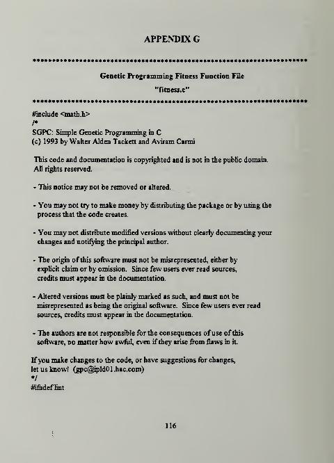
APPENDIX G
***********************************************************************
Genetic Programming Fitness Function File
"fitness.c"
***********************************************************************
^include <math.h>/*
SGPC: Simple Genetic Programming in C(c) 1993 by Walter Alden Tackett and Aviram Carmi
This code and documentation is copyrighted and is not in the public domain.
All rights reserved.
• This notice may not be removed or altered.
- You may not try to make money by distributing the package or by using the
process that the code creates.
- You may not distribute modified versions without clearly documenting your
changes and notifying the principal author.
- The origin ofthis software must not be misrepresented, either by
explicit claim or by omission. Since few users ever read sources,
credits must appear in the documentation.
- Altered versions must be plainly marked as such, and must not be
misrepresented as being the original software. Since few users ever read
sources, credits must appear in the documentation.
- The authors are not responsible for the consequences ofuse ofthis
software, no matter how awful, even ifthey arise from flaws in it.
Ifyou make changes to the code, or have suggestions for changes,
let us know! ([email protected])
•/
#ifedefhnt
116

static char fitness_c_rcsidD- '$Id: fitness.c,v 2.8 1993/04/14 05: 19:57 gpc-avc Exp
gpc-avc $";
#endif
/*
*
* SLog: fitness.c,v S
•Revision 2.8 1993/04/14 05:19:57 gpc-avc* just a revision number change
•/
#mclude <stdio.h>
#include <malloc.h>
^include <errno.h>
#include "gpc.h"
#include EXPtfnchide VAL_EXPextern terminal_table_entry terminaMableD;
extern int terminaltablesz
;
extern int totalvars
;
extern int fitness_table_sz;
/* */
#ifdefANSI_FUNC
VOID define_fitness_cases(
int numpops,
int numgens,
popstruct *pop
)
#else
VOID define_fitness_cases(numpops.numgens,pop
)
int numpops;
int numgens;
pop_struct *pop;
#endif
{
#if0
/* this template makes all ofthe fitness cases the same for all
populations, but that isn't necessary */
int p,i;
float range;
numfc =10; /* number of fitness or training cases */
numtc =10; /* number oftest or validation cases */
range = 1.0;
117

fitness_cases_table = (float **) malloc(numpops*sizeof(float *));
test_cases_table = (float **) malloc(nun]pops*sizeof(float *));
fitness_cases_table__out = (float **) malloc(numpops*sizeof(float *));
test_cases_table_out = (float **) malloc(numpops*sizeof(float *));
for (p=0; p<numpops; p++) {
fitness_cases_table[p] = (float *) malloc(numfc * azeof(float));
test_cases_table[p] = (float *) malloc(numtc * sizeoflfloat));
fitness_cases_table_out[p] = (float *) malloc(numfc * azeof(float));
test_cases_table_out[p] = (float *) malloc(numlc * sizeof(float));
for (i=0; i<numfc; i++) {
/* evenly spaced zero^'range': */
fitness_cases_table[p][i] = range * (float )i / (float)numfc;
/* evenly spaced 'range' about zero:
fitness_cases_table[p][i] = (2.0*range*(float)i/(float)numfc)-range;
*/
fitness_cases_table_out[p][i] =
regression_fiinction(fitness_cases_table[p][i]);
}
for (i=0; i<numtc; i++) {
/* validation test cases same as the training set */
test_cases_table[p][i] = fitness_cases_table[p][i];
/* validation could be random within the range:
test_cases_table[p][i] = random float(range);
or range centered about zero:
test_cases_table[p][i] = random_float(2.0*range)-range;
•/
test_cases_table_out[p][i] = regression_function(test_cases_table[p][i]);
)
)
#endif
/* no processing needed - we've got data! */
>
#ifdefANSI_FUNC
VOID evahiate_fitness_of_populations(
int numpops,
int numgens,
pop_struct*pop,
int p
)
#else
VOID evaluate_fitness_of_popubtions(numpops,numgens,pop,p)
int numpops;
int numgens;
118
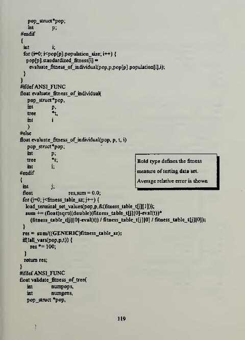
pop_struct*pop;
int p;
#endif
{
int i;
for (i=0; i<pop[p].population_size; i++) {
pop[p] . standardized_fitn ess[i] =
evahiate_toess_of_individual(pop,p,pop[p].population[i],i);
}
}
#ifdefANSI_FUNCfloat evaluate_fitness_of_mdrviduaI(
pop_stmct*pop,
int p,
tree *t,
int i
)
#else
float evahiate_fitness_of_individual(pop, p, t, i)
pop_struct*pop;
int p;
tree *t;
int i;
Bold type defines the fitness
measure oftesting data set.
Average relative error is shown
#endif
{
int j;
float res,sum = 0.0;
for(j=0;j<fitness_table_sz;j++) {
loadjerminal_set_values(pop,p,&(fitness_table_t[j][l]));
turn += (float)sqrt((double)(fitness_table_t[j]|0]-eva](t))*
(fitness table tU]I01-eval(t))/fitness_table_tlj]|0) /fitness_table_tyi[0]);
}
res = sum/((GENERIC)fitness_tabIe_sz);
in^!all_vars(pop,p,t)) {
res *= 100;
}
return res;
}
#ifdefANSI_FUNC
float validate_fitness_of_tree(
int numpops,
int numgens,
pop_struct *pop,
119

int p,
tree *t
)
#else
float vahdate_rmiess_of_tree(numpops, numgens, pop, p, t)
int numpops;
int numgens;
pop_struct *pop;
int p;
tree *t;
#endif
{
mt j;
float res, sum = 0.0;
float ev;
extern int val_fitness_table_sz;
for(j=0;j<val_fitness_table_sz;j-H-) {
load_terminal_set_values(pop,p,&(val_fitness_table_t[j] [ 1 ] ));
ev = eval(t);
sum += (float)sqrt((double)(val_fitness_table_t[jj[01-ev)*
(val_fitness_table_tljl|01-ev) / val_fitness_table_tij]|01 /
val_fitness_table_tlj] [0]);
}
res = sum/((GENERIC)val__fitness_table_sz);
if(!all_vars(pop,p,t)) {
res *= 100;
>
return res;
#ifdefANSI_FUNC
int terminate_earry(
int numpops,
int numgens,
popstruct *pop
)
#else
int terminate_early(numpops,numgens,pop)
int numpops;
int numgens;
popstruct *pop;
#endif
L
Bold type defines the fitness measure of
testing data set. Average relative error
is shown.
120

mt p,i;
for (p=0; p<numpops; p++) {
for (i=0; i<pop[p].population_size; i++) {
if(pop[p].standardized_fitness[i] <= 0.0) {
return 1;
>
>
}
return 0:
***********************************************************************
Genetic Programming Training Data Input File
COCOMO Training and Testing Version
"cotr42.c"
***********************************************************************
^include <stdio.h>
#inchide "gpc.h"
#inchide "prob.h"
#includeMcotr42.h"
GENERIC random_constant();
terminal_table_entry terminal_table[] = {
{0,MXO",random_constant},
{1,MXr',random_constant},
{2, "X2",random_constant},
{3,MX3 M
,random_constant},
{4, "X4",random_constant},
{5,wX5",random_constant},
{6,MX6",random_constant},
{7, "X7",random_constant},
(8, "X8",random_constant},
{9, "X9",random_constant},
{10,,,X10",random_constant},
{ 1 1 , "X 1 1 ",random_constant }
,
{12,wX12Vandom_constant},
{13,MX13 M
,random_constant},
{ 1 4, "X 14",random_constant }
,
{15, "X15",random_constant},
X0 = KDSI
X1=AAF
X2 through X 16 are the
cost driver values, RELY
through SCED.
121

{16, "X16",random_constant},
{0,FORMAT,random_constant }
,
>;
int tenninal_table_sz = sizeof(termmal_table)/si2eof(termmal_table_cntiy) - 1;
int totaljvars = FITNESS_HEIGHT;GENERIC toess_Ublej[FITNESS_WIDTH][FITNESS_HEIGHT] =
{ {2040.0000,
113.0000, 1.0000, 0.8800, 1.1600, 0.7000, 1.0000,
1.0600, 1.1500, 1.0700, 1.1900, 1.1300, 1.1700,
1.1000, 1.0000, 1.2400, 1.1000, 1.0400, },
{243.0000, 132.0000, 1.0000, 1.0000, 1.1600,
0.8500, 1.0000, 1.0000, 0.8700, 0.9400, 0.8600,
0.8200, 0.8600, 0.9000, 0.9500, 0.9100, 0.9100,
1.0000, >,
{240.0000, 60.0000, 0.7600, 0.7500, 1.1600,
0.7000, 1.0000, 1.0000, 0.8700, 1.0000, 1.1900,
0.9100, 1.4200, 1.0000, 0.9500, 1.2400, 1.0000,
1.0400, },
{33.0000, 16.0000, 1.0000, 0.8800, 0.9400,
1.0000, 1.0000, 1.0000, 0.8700, 1.0000, 1.0000,
1.0000, 0.8600, 0.9000, 0.9500, 1.2400, 1.0000,
1.0000, },
{423.0000, 30.0000, 1.0000, 1.1500, 0.9400,
1.3000, 1.3000, 1.2100, 1.1500, 1.0000, 0.8600,
1.0000, 0.8600, 1.1000, 1.0700, 0.9100, 1.0000,
1.0000, },
{321.0000, 29.0000, 0.6300, 1.4000, 0.9400,
1.3000, 1.1100, 1.5600, 1.0000, 1.0700, 0.8600,
0.8200, 0.8600, 0.9000, 1.0000, 1.0000, 1.0000,
1.0000, },
{218.0000, 32.0000, 0.6300, 1.4000, 0.9400,
1.3000, 1.1100, 1.5600, 1.0000, 1.0700, 0.8600,
0.8200, 0.8600, 0.9000, 1.0000, 1.0000, 1.0000,
1.0000, },
{40.0000, 6.1000, 0.6000, 1.4000, 1.0000,
1.3000, 1.3000, 1.5600, 1.0000, 0.8700, 0.8600,
1.0000, 0.8600, 1.0000, 1.0000, 1.0000, 1.0000,
1.0000, },
{6400.0000, 299.0000, 0.9600, 1.4000, 1.0800,
1.3000, 1.1100, 1.2100, 1.1500, 1.0700, 0.7100,
0.8200, 1.0800, 1.1000, 1.0700, 1.2400, 1.0000,
1.0800, },
122
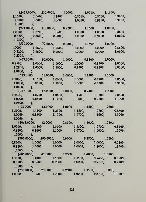
{2455.0000, 252.0000, 1.0000, 1.0000, 1.1600,
1.1500, 1.0600, 1.1400, 0.8700, 0.8700, 0.8600,
1.0000, 1.0000, 1.0000, 1.0000, 0.9100, 0.9100,
1.0000, },
{724.0000, 118.0000, 0.9200, 1.1500, 1.0000,
1.0000, 1.2700, 1.0600, 1.0000, 1.0000, 0.8600,
0.8200, 0.8600, 0.9000, 1.0000, 0.9100, 1.0000,
1.2300, },
{539.0000, 77.0000, 0.9800, 1.1500, 1.0000,
1.0000, 1.0800, 1.0600, 1.0000, 1.0000, 0.8600,
0.8200, 0.8600, 0.9000, 1.0000, 1.0000, 1.0000,
1.2300, },
{453.0000, 90.0000, 1.0000, 0.8800, 1.0000,
0.8500, 1.0600, 1.0600, 1.0000, 0.8700, 1.0000,
1.2900, 1.0000, 1.1000, 0.9500, 0.8200, 0.8300,
1.0000, },
{523.0000, 38.0000, 1.0000, 1.1500, 1.1600,
1.3000, 1.1500, 1.0600, 1.0000, 0.8700, 0.8600,
1.0000, 0.8600, 1.1000, 1.0000, 0.8200, 0.9100,
1.0800, >,
{387.0000, 48.0000, 1.0000, 0.9400, 1.0000,
0.8500, 1.0700, 1.0600, 1.1500, 1.0700, 0.8600,
1.0000, 0.8600, 1.1000, 1.0000, 0.9100, 1.1000,
1.0800, },
{98.0000, 13.0000, 1.0000, 1.1500, 1.0800,
1.3000, 1.1100, 1.2100, 1.1500, 1.0700, 0.8600,
1.0000, 0.8600, 1.1000, 1.0700, 1.1000, 1.1000,
1.0000, },
{1063.0000, 62.0000, 0.8100, 1.4000, 1.0800,
1.0000, 1.4800, 1.5600, 1.1500, 1.0700, 0.8600,
0.8200, 0.8600, 1.1000, 1.0700, 1.0000, 1.0000,
1.0000, },
{702.0000, 390.0000, 0.6700, 0.8800, 1.0800,
0.8500, 1.0000, 1.0000, 1.0000, 1.0000, 0.7100,
0.8200, 1.0000, 1.0000, 1.0000, 1.1000, 1.1000,
1.0000, },
{605.0000, 42.0000, 0.9600, 1.4000, 1.0800,
1.3000, 1.4800, 1.5600, 1.1500, 0.9400, 0.8600,
0.8200, 0.8600, 0.9000, 1.0000, 0.9100, 0.9100,
1.0000, },
{230.0000, 23.0000, 0.9600, 1.1500, 1.0800,
1.0000, 1.0600, 1.0000, 1.0000, 0.8700, 1.0000,
123
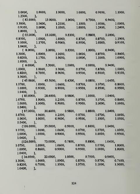
1.0000, 1.0000, 1.0000, 1.0000, 0.9100, 1.1000,
1.2300, },
{82.0000, 13.0000, 1.0000, 0.7500, 0.9400,
1.3000, 1.0600, 1.2100, 1.1500, 1.0000, 1.0000,
0.9100, 1.0000, 1.1000, 1.0000, 1.2400, 1.2400,
1.0000, },
{55.0000, 15.0000, 0.8100, 0.8800, 1.0800,
0.8500, 1.0000, 1.0000, 0.8700, 0.8700, 1.1900,
1.0000, 1.1700, 0.9000, 0.9500, 1.0000, 0.9100,
1.0400, },
{ 8.0000, 3.0000, 0.8300, 1.0000, 0.9400,
1.3000, 1.0000, 1.0000, 1.0000, 0.8700, 0.8600,
0.8200, 1.1700, 1.0000, 1.0000, 1.1000, 1.0000,
1.0000, },
{ 6.0000, 5.3000, 1.0000, 0.8800, 0.9400,
1.0000, 1.0000, 1.0000, 0.8700, 0.8700, 1.0000,
0.8200, 0.7000, 0.9000, 0.9500, 0.9100, 0.9100,
1.0000, >,
{45.0000, 45.5000, 0.4300, 0.8800, 1.0400,
1.0700, 1.0000, 1.0600, 0.8700, 1.0700, 0.8600,
1.0000, 0.9300, 0.9000, 0.9500, 0.9500, 0.9500,
1.0400, >,
{ 83.0000, 28.6000, 0.9800, 1.0000, 1.0400,
1.0700, 1.0000, 1.2100, 0.8700, 1.0700, 0.8600,
1.0000, 1.0000, 0.9000, 0.9500, 1.0000, 1.0000,
1.0400, },
{87.0000, 30.6000, 0.9800, 0.8800, 1.0400,
1.0700, 1.0600, 1.2100, 0.8700, 1.0700, 1.0000,
1.0000, 1.0000, 0.9000, 0.9500, 1.1000, 1.0000,
1.0400, },
{106.0000, 35.0000, 0.9100, 0.8800, 1.0400,
1.0700, 1.0000, 1.0600, 0.8700, 1.0700, 1.0000,
1.0000, 1.0000, 0.9000, 0.9500, 1.0000, 0.9500,
1.0400, },
{126.0000, 73.0000, 0.7800, 0.8800, 1.0400,
1.0700, 1.0000, 1.0600, 0.8700, 1.0700, 1.0000,
1.0000, 0.8600, 0.9000, 0.9500, 1.0000, 1.0000,
1.0400, },
{36.0000, 23.0000, 1.0000, 0.7500, 0.9400,
1.3000, 1.0000, 1.0000, 0.8700, 0.8700, 0.7100,
0.8200, 0.7000, 1.1000, 1.0700, 1.1000, 1.0000,
1.0400, },
124

{1272.0000, 464.0000, 0.6700, 0.8800, 0.9400,
0.8500, 1.0000, 1.0000, 0.8700, 1.0000, 1.1900,
0.9100, 1.1700, 0.9000, 0.9500, 1.1000, 1.0000,
1.0400, >,
{156.0000, 91.0000, 1.0000, 1.0000, 1.0000,
0.8500, 1.0000, 1.0000, 1.0000, 0.8700, 0.7100,
1.0000, 0.7000, 1.1000, 1.0000, 0.8200, 0.9100,
1.0000, },
{176.0000, 24.0000, 1.0000, 1.1500, 1.0000,
1.0000, 1.3000, 1.2100, 1.0000, 0.8700, 0.8600,
1.0000, 0.8600, 1.1000, 1.0000, 1.0000, 1.0000,
1.0000, },
{122.0000, 10.0000, 1.0000, 0.8800, 1.0000,
1.0000, 1.0000, 1.0000, 1.0000, 1.1500, 1.1900,
1.0000, 1.4200, 1.0000, 0.9500, 1.2400, 1.1000,
1.0400, },
{ 14.0000, 5.3000, 1.0000, 0.8800, 0.9400,
1.1500, 1.1100, 1.2100, 1.3000, 1.0000, 0.7100,
1.0000, 0.7000, 1.1000, 1.0700, 1.0000, 1.1000,
1.0800, },
{20.0000, 4.4000, 1.0000, 1.0000, 0.9400,
1.0000, 1.0000, 1.0600, 1.1500, 0.8700, 1.0000,
0.8200, 1.0000, 1.0000, 0.9500, 0.9100, 1.1000,
1.0000, },
{ 18.0000, 6.3000, 1.0000, 0.8800, 0.9400,
0.7000, 1.0000, 1.0000, 0.8700, 0.8700, 0.8600,
0.8200, 1.1700, 0.9000, 0.9500, 1.1000, 1.0000,
1.0000, },
{958.0000, 27.0000, 1.0000, 1.1500, 0.9400,
1.3000, 1.3000, 1.2100, 1.0000, 1.0000, 0.8600,
0.9100, 1.0000, 1.1000, 1.0700, 1.1000, 1.1000,
1.0800, },
{237.0000, 17.0000, 0.8700, 1.0000, 0.9400,
1.1500, 1.1100, 1.2100, 1.3000, 1.0000, 1.0000,
1.0000, 1.0000, 1.1000, 1.0700, 1.1000, 1.1000,
1.2300, },
{130.0000, 25.0000, 1.0000, 1.4000, 0.9400,
1.3000, 1.6600, 1.2100, 1.0000, 1.0000, 0.7100,
0.8200, 0.7000, 0.9000, 0.9500, 0.9100, 1.0000,
1.0000, },
{38.0000, 9.1000, 1.0000, 0.8800, 0.9400,
1.3000, 1.1100, 1.2100, 1.1500, 1.0000, 0.7800,
125

0.8200, 0.7000, 1.2100, 1.1400, 0.9100, 1.2400,
1.0000, },
{ 15.0000, 10.0000, 1.0000, 1.0000, 0.9400,
1.1500, 1.0000, 1.0000, 1.0000, 0.8700, 0.7100,
0.8200, 0.8600, 1.0000, 1.0000, 0.8200, 1.0000,
1.0000, },
};
int fitness_table_sz = FTTNESS_WIDTH;GENERIC fitoessjable[FITNESS_HEIGHTl[FITNESS_WIDTH];
***********************************************************************
Perl Script for Creating Genetic Programming Input Training Data File
"defincpr
(Author: Ranjan Bagchi)***********************************************************************
#!/pubhc/gnu/bin/perl —
# define — generates static data instantiating all necessary
# terminals.
Sfirst = 0;
Soutf= $ARGV[0];
openCOUT/^Soutfc");
open(OUT_h,">$out£h");
while<o){
if(/A\w*$/) {
next;
}
@l = spht(");
ntSfirst= 0) {
print OUT"#inchide <stdio.h>\n",
"tfnchideV'gpc.hVW,M#mchide\ ,,
prob.h\,,
\nM,
sprintfi;"#include \,,
%s.h\"\n,,
,$outf),
"\nGENERIC random_constant();\n"
print OUT•'terminaltableentry terminaltableQ = {\n*
for(0..$#l-l) {
126
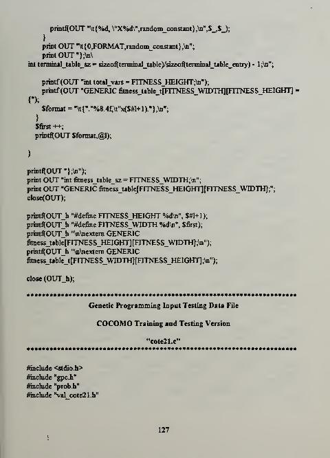
printf(OUT "\t{%d, \"X%d\",random_constant}>",$_,$_);
)
print OUT ,
'\t{0,FORMAT,random_constant},\n";
print OUT "};\n\
int tenninal_table_sz = sizeon^tennmal_tableysizeof(tenmnal_Uble_cntiy) - l;\n";
printf(OUT "int totaljvars = FITNESS_HEIGHT;\nM);
printf(OUT "GENERIC toessjablej[FITNESS_WroT71]|TlTNESS_HEIGHT] =
Sformat = "\t{"."%8.4f;\tMx($#l+l)."},\n";
>
$first++;
printf(OUT $fonnat,@I);
>
printf(OUT"};\n");
print OUT "int fitness_table_sz = FTTNESS_WIDTH;\n";
print OUT "GENERIC fitness_table[FITNESS_HEIGHT|[FITNESS_WIDTH];";
close(OUT);
printf(OUT_h "tfdefine FITNESS_HEIGHT %d\n", $#1+1);
printf(OUT_h "#define FTTNESS_WIDTH %d\n", Sfirst);
printf(OUT_h "\n\nextern GENERICtoessjable[FTmESS_HEIGHT][ITrNESS_WIDTH];\n");
printflOUT_h "\n\nextem GENERICfitoess_Ublej[FTT>IESS_WIDTH][FITNESS_HEIGHT];\n");
close (OUT_h);
***********************************************************************
Genetic Programming Input Testing Data File
COCOMO Training and Testing Version
"cote21.c"***********************************************************************
#inchide <stdio.h>
#inchide "gpc.h"
#inchide "prob.h"
#inchide "val cote21.h"
127

GENERIC val_toessjablej[VAL_FITNESS_WIDTH][VAL_FITNESS_HEIGHT] ={
{1600.0000, 293.0000, 0.8500, 0.8800, 1.1600, 0.8500,
1.0000, 1.0600, 1.0000, 1.0700, 1.0000, 0.9100,
1.0000, 0.9000, 0.9500, 1.1000, 1.0000, 1.0000,
},
{43.0000, 4.0000, 1.0000, 0.7500, 1.0000,
0.8500, 1.0000, 1.2100, 1.0000, 1.0000, 1.4600,
1.0000, 1.4200, 0.9000, 0.9500, 1.2400, 1.1000,
1.0000, },
{ 8.0000, 6.9000, 1.0000, 0.7500, 1.0000,
1.0000, 1.0000, 1.0000, 0.8700, 0.8700, 1.0000,
1.0000, 1.0000, 0.9000, 0.9500, 0.9100, 0.9100,
1.0000, },
{1075.0000, 22.0000, 1.0000, 1.1500, 0.9400,
1.3000, 1.6600, 1.5600, 1.3000, 1.0000, 0.7100,
0.9100, 1.0000, 1.2100, 1.1400, 1.1000, 1.1000,
1.0800, },
{201.0000, 37.0000, 1.0000, 1.1500, 0.9400,
1.3000, 1.1100, 1.0600, 1.0000, 1.0000, 0.8600,
0.8200, 0.8600, 1.0000, 0.9500, 0.9100, 1.0000,
1.0800, },
{79.0000, 25.0000, 0.9600, 1.1500, 0.9400,
1.3000, 1.1100, 1.0600, 1.1500, 1.0000, 0.7100,
1.0000, 0.7000, 1.1000, 1.0000, 0.8200, 1.0000,
1.0000, },
{73.0000, 3.0000, 1.0000, 1.1500, 0.9400,
1.6500, 1.3000, 1.5600, 1.1500, 1.0000, 0.8600,
1.0000, 0.7000, 1.1000, 1.0700, 1.1000, 1.2400,
1.2300, },
{61.0000, 3.9000, 1.0000, 1.4000, 0.9400,
1.3000, 1.3000, 1.0600, 1.1500, 0.8700, 0.8600,
1.1300, 0.8600, 1.2100, 1.1400, 0.9100, 1.0000,
1.2300, },
{ 9.0000, 3.6000, 0.5300, 1.4000, 1.0000,
1.3000, 1.3000, 1.5600, 1.0000, 0.8700, 0.8600,
0.8200, 0.8600, 1.0000, 1.0000, 1.0000, 1.0000,
1.0000, },
{11400.0000, 320.0000, 1.0000, 1.1500, 1.1600,
1.1500, 1.3000, 1.2100, 1.0000, 1.0700, 0.8600,
1.0000, 1.0000, 1.0000, 1.0000, 1.2400, 1.1000,
1.0800, },
{6600.0000, 1150.0000, 0.8400, 1.1500, 1.0800,
1.0000, 1.1100, 1.2100, 0.8700, 0.9400, 0.7100,
128

0.9100, 1.0000, 1.0000, 1.0000, 0.9100, 0.9100,
1.0000, },
{88.0000, 9.4000, 1.0000, 1.1500, 0.9400,
1.1500, 1.3500, 1.2100, 1.0000, 0.8700, 1.0000,
1.0000, 1.0000, 1.0000, 1.0000, 0.8200, 1.1000,
1.0800, },
{ 7.3000, 2.1400, 1.0000, 0.8800, 1.0000,
1.0000, 1.0000, 1.0000, 1.0000, 1.0000, 1.1000,
1.2900, 0.8600, 1.0000, 1.0000, 0.9100, 0.9100,
1.2300, },
{ 5.9000, 1.9800, 1.0000, 0.8800, 1.0000,
1.0000, 1.0000, 1.0000, 1.0000, 1.0000, 1.0000,
1.2900, 0.8600, 1.0000, 1.0000, 0.9100, 0.9100,
1.2300, },
{47.0000, 60.0000, 0.5600, 0.8800, 0.9400,
0.7000, 1.0000, 1.0600, 1.0000, 1.0000, 0.8600,
0.8200, 0.8600, 1.0000, 1.0000, 1.0000, 1.0000,
1.0000, },
{ 12.0000, 15.0000, 1.0000, 1.0000, 1.0000,
1.1500, 1.0000, 1.0000, 0.8700, 0.8700, 0.7100,
0.9100, 1.0000, 0.9000, 0.9500, 0.8200, 0.9100,
1.0000, },
{ 8.0000, 6.2000, 1.0000, 1.0000, 1.0000,
1.1500, 1.0000, 1.0000, 0.8700, 1.0000, 0.7100,
0.8200, 0.7000, 1.0000, 0.9500, 0.9100, 1.1000,
1.0000, },
{41.0000, 8.2000, 1.0000, 0.8800, 0.9400,
0.8500, 1.0000, 1.0600, 1.1500, 1.0000, 1.0000,
1.0000, 1.0000, 1.1000, 1.0700, 1.2400, 1.1000,
1.0000, >,
{70.0000, 23.0000, 0.9000, 1.0000, 0.9400,
1.1500, 1.0600, 1.0600, 1.0000, 0.8700, 1.0000,
1.0000, 1.0000, 1.0000, 1.0000, 0.9100, 1.0000,
1.0000, },
{57.0000, 6.7000, 1.0000, 1.1500, 0.9400,
1.3000, 1.1100, 1.0600, 1.0000, 1.0000, 0.8600,
1.1300, 0.8600, 1.1000, 1.0700, 1.1000, 1.1000,
1.0800, },
{50.0000, 28.0000, 1.0000, 1.0000, 0.9400,
1.1500, 1.0000, 1.0000, 0.8700, 0.8700, 0.8600,
1.0000, 0.8600, 0.9000, 1.0000, 0.8200, 1.0000,
1.0000, >,
>;
129

int val_fitness_table_sz = VAL_FTmESS_WIDTH;GEh^RICval_fitnessjable[VAL_nTNESS_HEIGHT][VAL_FITNESS_WIDTH];***********************************************************************
Perl Script for Creating Genetic Programming Input Testing Data File
"val_define.pr
(Author: Ranjan Bagchi)
***********************************************************************
#!/pubhc/gnu/bin/perl ~
U define — generates static data instantiating all necessary
# terminals.
Sfirst = 0;
Soutf= "val_$ARGV[0]M;
open(OUT,">$outf.c");
open(OUT_h,">$out£h");
while<<>){
in7A\w*$/) {
next;
>
@l = spbt(");
if($first= 0) {
print OUT"#include <stdio.h>\n",
"#include Vgpc.hVV,"^include V'prob.hW,
sprintn:"#include\"%s.h\"\n,,
,$outf),
"GENERICval_fiHnessjablej[VAL_FITNESS_WroTH][VAL_nTNESS_HEIGHT| = {";
Sformat = "\t{VToS^fX'x^l+l)."},^";
}
Sfirst ++;
printf(OUT $format,@l);
}
printn;OUT"};\n");
print OUT "int val_fitness_table_sz = VAL_FTTNESS_WIDTH;\n";
print OUT "GENERICval_fitoessjable[VAL_Fn7^SS_HEIGHT][VAL_FrrNESS_WIDTH];";
130
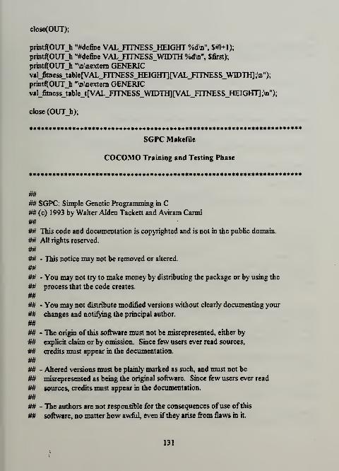
close(OUT);
printfJOUTJiM#define VALJTTNESS_HEIGHT %d\n", $#1+1);
printf(OUTh "#define VAL_FTTNESS_WIDTH %d\n", Sfirst);
printflOUTJi "\n\nextern GENERICval_fitoessJable[VAL_FITNESS_HEIGH^^[VAL_FITNESS_WIDTH];\n ,,
);
printf(OUT_h "\n\nextern GENERICval_toessJableJ[VAL_F^^^^SS_WroTH][VAL_FITNESS_HEIGHTl;\Il
,,
);
close (OUT_h);
**********************************************************************
SGPC Makefile
COCOMO Training and Testing Phase
**********************************************************************
##
## SGPC: Simple Genetic Programming in CM (c) 1993 by Waher Alden Tackett and Aviram Carmi
m## This code and documentation is copyrighted and is not in the public domain.
## All rights reserved.
##
## - This notice may not be removed or altered.
m## - You may not try to make money by distributing the package or by using the
## process that the code creates.
m## - You may not distribute modified versions without clearly documenting your
## changes and notifying the principal author.
##
## - The origin ofthis software must not be misrepresented, either by
## explicit claim or by omission. Since few users ever read sources,
## credits must appear in the documentation.
##
## - Altered versions must be plainly marked as such, and must not be
## misrepresented as being the original software. Since few users ever read
## sources, credits must appear in the documentation.
##
## - The authors are not responsible for the consequences ofuse ofthis
ffl software, no matter how awful, even ifthey arise from flaws in it.
131

mffl Ifyou make changes to the code, or have suggestions for changes,
## let us know! ([email protected])
# Sid: Makefiles 1.1 1993/04/30 05:01:48 gpc-avc Exp gpc-avc $
#
# invoke this Makefile with the command: make [ TYPE=type ]
U
# where you have the problem-specific fitness and setup files named
# fitness c and setup.
c
U
# TYPE should usually equal int or float, but in principle can be anything.
U
# SLog: Makefiles $
# Revision 1.1 1993/04/30 05:01:48 gpc-avc
# Initial revision
§
# Revision 1.7 1993/04/23 01:56:25 gpc-avc
TYPE = float
DEBUG =
EXP"cotr42VALJEXP-val_cote21FLAGS - -O -DTYPE=$(TYPE) -DDEBUG=$(DEBUG)-DVAL_EXI^\"S(VAL_EXP).h\"-DEXP=\"$(EXP).h\"
SRCS = setup.c fitoess.c $(EXP).c main.c S(VAL_EXP).c
INCS - prob.h
OBJS = $(SRCS:%.c=%.o)
EXE =gpc-l$(PROBLEM)
## NOTE: last definition wins ##
CC = gcc
CFLAGS= -g-I.Vlib
#CFLAGS = -0-I../lib
CPPFLAGS = $(FLAGS)
LIBS = -L../lib -lgpcS(TYPE) -lm
Bold type indicates problem specific
declarations that include the COCOMO
training and testing files created by
define.pl and val_define.pl
132

gcc cc debug-cc debug-gcc purify prof all: $(OBJS)
(cd../lib;\
$(MAKE) TYPE=$(TYPE) DEBUG=$(DEBUG) \
CC=$(CC) CFLAGS="$(CFLAGS)" $@)$(CC) -o $(EXE) $(OBJS) $(LIBS)
clean:
/bin/rm -f$(EXE) $(OBJS) Makefile.bak
real-clean: clean
(cd../lib;\
$(MAKE) TYPE=$(TYPE) DEBUG=$(DEBUG) \
CC=$(CC) CFLAGS=-$(CFLAGS)Mclean)
print:
co:
ci:
rwf-s7 -1 -pM-2 -f -m -t8 $(SRCS) $(INCS)
|Ipr
(cd../m>;\
$(MAKE) TYPE=$(TYPE) DEBUG=$(DEBUG) \
CC=$(CC) CFLAGS=M$(CFLAGS)" $@)
-co -1 $(SRCS) $(INCS) Makefile
(cd../lib;\
$(MAKE) TYPE=$(TYPE) DEBUG=$(DEBUG) \
CC=$(CC) CFLAGS=M$(CFLAGS)" $@)
-ci -1 $(SRCS) $(INCS) Makefile
(cd../Kb;\
$(MAKE) TYPE=$(TYPE) DEBUG=$(DEBUG) \
CC=$(CC) CFLAGS="$(CFLAGS)M$@)
lint
$(LINT.c) $(CFLAGS) $(FLAGS) $(SRCS)
(cd../lib;\
$(MAKE) TYPE=$(TYPE) DEBUG=$(DEBUG) \
CC=$(CC) CFLAGS="$(CFLAGS)" $@)
depend:
makedepend - $(CFLAGS) -- $(FLAGS) $(SRCS)
(cd../lib;\
$(MAKE) TYPE=$(TYPE) DEBUG=$(DEBUG) \
133

CC=$(CC) CFLAGS="$(CFLAGS)" $@)
# DO NOT DELETE THIS LINE - make depend depends on h.
setup.o: /usr/mchide/stdio.h ../lib/gpc.h ../lib/proto.h ../lib/random.
h
setup. o: prob.h
fitness. o: /usr/mchide/stdio.h /usr/include/maUoch /usr/inchide/ermo.h
fitness.o: /usr/mchide/sys/ermo.h ../lib/gpc.h ../lib/proto.h
fitness.o: ../lib/random.h
134

LIST OF REFERENCES
Boehm, B. W., Software Engineering Economics, Prentice-Hall, Inc., Englewood Cliffs,
NJ, 1981.
Boehm, B. W. , "Software Engineering Economics," IEEE Transactions on Software
Engineering, SE-10, 1, pp. 4-21, January 1984.
Boehm, B. W., "Survey and Tutorial Series—Improving Software Productivity,"
Computer, September 1987, pp. 43-57.
California Scientfic Software, BrainMaker Reference Manual, 1992.
California Scientific Software, BrainMaker Genetic Training Option Reference Manual,
1993.
Eberhart, R.C., and Dobbins, R.W., Neural Network PC Tools: A Practical Guide,
Academic Press Inc., San Diego CA, 1990.
Goldberg, D. E., Genetic Algorithms in Search, Optimization, and Machine Learning,
Addison-Wesley Publishing Company, Inc., Reading MA, 1989.
Holland, J. H., "Genetic Algorithms," Scientific American, July 1992, pp. 66-72.
Kemmerer, C. F., "An Empirical Validation of Software Cost Estimation Models,"
Communications oftheACM, v. 30, no. 5 (May 1987), pp. 416-429.
Koza, J. R., Genetic Programming: On the Programming ofComputers by Means ofNatural Selection, The MIT Press, Cambridge, MA, 1992.
Maren, A., Harston, C, and Pap, R_, Handbook ofNeural Computing Applications,
Academic Press Inc., San Diego, CA, 1990.
University of California, San Diego, Report CS92-249, A User's Guide to GAucsd 1.4, by
N. N. Schraudolph and J. J. Grefenstette, pp. 1-23, 7 July 1992.
Zahedi, F., "An Introduction to Neural Networks and a Comparison with Artificial
Intelligence and Expert Systems," INTERFACES, 21:2 (March-April 1991), pp. 25-38.
135

INITIAL DISTRIBUTION LIST
1. Defense Technical Information Center
Cameron Station
Alexandria, VA 22304-6145
2. Library, Code 52
Naval Postgraduate School
Monterey, CA 93943-5002
3. Dr. Balasubramanium Ramesh, Code AS/RADepartment of Administrative Sciences
Naval Postgraduate School
Monterey, CA 93943-5000
4. Dr. Tarek K. Abdel-Hamid, Code AS/AHDepartment ofAdministrative Sciences
Naval Postgraduate School
Monterey, CA 93943-5000
5. LT MichaelA Kelly
1216 Sylvan Rd.
Roanoke, VA 24014
-j0<?
136


HS/pLfcY KNOX LIBRARY

Top Related