


Languages
Pages
Legal

A First and Second Order Moment Approach
to Probabilistic Control Synthesis
Luis G. Crespo ∗
National Institute of Aerospace, Hampton, VA, 23666, USA
Sean P. Kenny †
Dynamic Systems and Control Branch, NASA LaRC, Hampton, VA, 23681
This paper presents a robust control design methodology based on the
estimation of the first two order moments of the random variables and
processes that describe the controlled response. Synthesis is performed by
solving an multi-objective optimization problem where stability and perfor-
mance requirements in time- and frequency- domains are integrated. The
use of the first two order moments allows for the efficient estimation of the
cost function thus for a faster synthesis algorithm. While reliability re-
quirements are taken into account by using bounds to failure probabilities,
requirements related to undesirable variability are implemented by quanti-
fying the concentration of the random outcome about a deterministic target.
The Hammersley Sequence Sampling and the First- and Second-Moment-
Second-Order approximations are used to estimate the moments, whose
accuracy and associated computational complexity are compared numeri-
cally. Examples using output-feedback and full-state feedback with state
estimation are used to demonstrate the ideas proposed.
∗Staff Scientist, 144 Research Drive, Hampton VA 23666, AIAA Professional Member†Aerospace Technologist, Dynamic Systems and Control Branch, NASA LaRC, Hampton VA 23681
1 of 34
https://ntrs.nasa.gov/search.jsp?R=20050232742 2018-07-27T06:59:02+00:00Z

I. Introduction
Achieving balance between stability and performance in the presence of uncertainties is
one of the fundamental challenges faced by control engineers. Trade-offs must be made to
reach acceptable levels of stability and performance with adequate robustness to parameter
uncertainty. These trade-offs are explicitly linked to the control engineer’s choice of uncer-
tainty model as well as how that model is exploited in the synthesis process. Usually, the
assumed uncertainty model has a profound impact on the performance robustness of the
closed-loop system.
Several uncertainty models, such as norm-bounded perturbations, interval analysis, fuzzy
sets, and probabilistic methods1–3 are typically used. The most commonly used robust
control methods4 are µ-synthesis and H-infinity. In these methods, uncertainty is modeled
with norm-bounded complex perturbations of arbitrary structure about a nominal plant.
This treatment is used primarily because it leads to a tractable set of sufficient conditions
for robust stability, making the approach computationally efficient. These methods are based
on the most pessimistic value of performance among all possible ones, usually referred to
as “worst-case”. This worst-case performance is usually realized only by a single member
of the uncertain model set and by a particular input signal. No information is provided
regarding the likelihood that this worst-case will ever occur in practice. In addition, the
intrinsic mathematical requirements of the approach usually lead to conservative models of
uncertainty, over-conservative designs and complicated compensators.
Probabilistic uncertainty not only defines a set of plants where the actual dynamic sys-
tem is assumed to reside but also associates a weight, the value of the probability density
function, to each member of the set. In contrast to conventional robust control methods, this
“additional dimension” allows the pursuit of robustly optimal solutions in the probabilistic
sense. For instance, reliability-based design searches for solutions that minimize the proba-
bility of violating design requirements prescribed in terms of inequality constraints. Hence,
reliability-based control design searches for the compensator that places as much probability
as possible within the region where the design requirements are satisfied. Notice that this
allows for the search of the compensator with the best robustness for a given control struc-
ture, e.g. the most robust PID controller. This can be achieved even though the violation of
some the design requirements for some of the plants in the uncertainty set is unavoidable.
Synthesis approaches based on random searches5,6, 14 and stochastic gradient algorithms8–10
2 of 34

have been applied to probabilistic robust control. In these studies, random sampling is the
primary tool for assessing and pursuing acceptable levels of robustness in the control solution.
On the other hand, asymptotic approximations11,12 for the estimation of failure probabili-
ties have only been used as a control analysis tool. Reference,13 foundation of this study,
integrates and extends some of these tools.
This paper is organized as follows. Section II presents basic concepts related to control
and probabilistic uncertainty. Section III introduces reliability metrics for random variables
and processes. Mean and variance based bounds to the reliability metrics are also derived
therein. Robustness-based metrics for random variables and processes are introduced in
Section IV. Section V presents the numerical methods used to estimate the above mentioned
metrics. The control synthesis procedure is presented in Section VI, where specifics of
both the reliability and the robustness-based formulations are examined. Two examples are
presented in Section VII, where a satellite’s attitude control problem and the disturbance
rejection in a flexible beam are used to demonstrate the method. Finally, some conclusions
are stated in Section VIII.
II. System Dynamics
Let p be a vector of random variables used to model the uncertain parameters of the
system. In this study, p is prescribed a priori by the joint probability density function
(PDF) fp(p) or equivalently by the cumulative distribution function (CDF) Fp(p)a. The set
of values that p could take, called the support of p, will be denoted as ∆p.
Consider the probabilistic model M(p) of a Linear Time Invariant (LTI) system, where
the dependence of the model on the uncertain parameters could be non-linear. The reader
must notice however, that the developments presented herein do not require the system to
be LTI. The propagation of ∆p through M leads to a set of uncertain plant models in which
the physical system is assumed to reside. The probability distribution of a plant within this
set is fully determined by M(p) and fp(p). In a transfer function representation, we will
refer to the uncertain plant as G(p) and to the compensator as K(k), where k is the vector
of design parameters to be determined. Alternatively, a state space realization of M(p)
aIn these expressions, the subscript refers to the symbol used for the random variable while the value inparenthesis refers to a particular realization.
3 of 34

leads to
x = A(p)x + B(p)u + F(p)z (1)
y = C(p)x + D(p)u + E(p)v (2)
where x is the state, u is the control, z is process noise, y is the system output and v is
sensor noise. The noise signals are commonly modeled as delta correlated Gaussian white
noises satisfying E[z] = 0 and E[z(t)zT (t + κ)] = Sδ(κ), where z = [zT ,vT ]T and S is a
constant spectral density matrix. In what follows, the explicit dependence of the matrices
in Equations (1-2) on p is omitted while D is assumed to be zero.
Important properties, typically used in control design, such as pole placement and the
Separation Principle, do not hold due to the offset between the deterministic mathematical
model and the actual dynamic system. The effects of parametric uncertainty on the Separa-
tion Principle are considered next. For the full-state feedback law u = −Gx and a full-order
observer with gain L based on the expected plant E[M(p)] (any other deterministic plant
such as M(E[p]) could be used instead), the closed-loop dynamics for full-state feedback is
given by
˙x = Ax + Bz (3)
y = Cx + Ez (4)
A =
A−BG BG
A− E[A] + (E[B]−B)G
+L(E[C]−C)(B− E[B])G + E[A]− LE[C]
B =
F 0
F −LE
where x is the estimation of x, x = [xT , eT ]T is the augmented state vector, e = x − x
is the estimation error, C = [CT |0T ]T and E = [0T |ET ]T . The vector k is formed by the
feedback gain G and the observer gain L. Notice that the Separation Principle holds, i.e.,
4 of 34

A is upper triangular, if the deterministic plant used to generate the observer matches the
physical dynamic system. Uncertainty in the plant makes the Separation Principle invalid.
In addition, the random closed-loop poles do not occur at the locations selected for the
full-state feedback, i.e. poles of the A1,1 subsystem, nor at the locations for the full-order
observer, i.e. poles of the A2,2 subsystem.
III. Reliability-Based Metrics
The propagation of a fixed set of parameters of the plant through conventional control
analysis tools leads to set of scalar quantities, e.g. closed loop poles, and a set of functions,
e.g. step responses, and Bode plots. The propagation of probabilistic uncertainty through the
same tools leads to random variables, e.g. random closed-loop poles, and random processes,
e.g. the step responses become random processes parameterized by time, and the Bode plots
become random processes parameterized by frequency. In this section we first introduce
reliability metrics for random variables and processes. These metrics will be used to quantify
the violation of the design requirements. Specific realizations corresponding to stability, time,
and frequency requirements are then provided. In general, we will use x and x(h) to denote
a random variable and a random process dependent on p through the plant model. For the
random process x(h), h refers to an arbitrary variable such as time or frequency.
A. Random Variables
We first introduce the concept of probability of failure. Let x(p) be the random variable of
interest. Let x > x be a design requirement. The event x ≤ x will be referred to as failure.
The corresponding failure set is given by F = {x | x ∈ (−∞, x]}, where the failure boundary
x is a deterministic quantity prescribed in advance. The admissible domain, namely A =
{x | x ∈ (x,∞)}, is the complement of the failure domain. The same type of discrimination
can be done in the parameter space p by using x(p). The function g(p, x) = x(p)−x, called
the limit state function, divides the parameter space in two parts, the domain leading to
A, i.e. g(p, x) > 0, and the domain leading to F , i.e. g(p, x) ≤ 0. Hence, F results from
mapping the set {p ∈ ∆p | g(p, x) ≤ 0} through x(p). In this case, the probability of failure
5 of 34

Pf is given by
Pf = P[x ≤ x] =
∫x≤x
fx(x)dx =
∫g≤0
fp(p)dp (5)
Similar expressions can be derived if the design requirement is x < x. These expressions
describe reliability metrics for the random variable x when a single constraint is present, i.e.,
x > x or x < x. A reliability metric for the random variable x having both constraints can
be easily formed
rx(x, x)∆= rx(x) + rx(x) (6)
where
rx(x)∆= P[x ≤ x] = Fx(x) (7)
rx(x)∆= P[x > x] = 1− Fx(x) (8)
Notice that rx(x) is equivalent to Pf in Equation (5). We will refer to x and x as the
boundaries of the failure domain F = {x | x ∈ (−∞, x]∪ (x,∞)}. Notice that the under-bar
and the over-bar refer to the bound from below and the bound from above of the admissible
domain A = {x | x ∈ [x, x)}. This convention will be used for the remainder of the paper.
Notice that the mapping of the corresponding limit state function through x(p) leads to the
failure boundary(s). Hence, there is a direct correspondence between F and g.
B. Random Processes
The random process x(h) can be considered as the parameterization of the random variable
x by the deterministic variable h. In this paper h ∈ [0,∞] is assumed. The random process
x(h) is specified by the set of CDFs15 Fx(h)(x, h). For instance, the system output y(t) is
prescribed by Fy(t)(y, t). The evaluation of the process at a particular h value, say hi, leads
to the random variable x(hi) whose CDF is given by Fx(x) = Fx(h)(x, hi). In general, the
support and the percentiles of x(h) vary with h.
Let x(h) > x(h) for h ∈ [h1, h2] and x(h) ≤ x(h) for h ∈ [h3, h4] be design requirements
for the random process x(h). In this paper, reliability metrics for processes are formulated
by extending the ideas presented above. This is attained by integrating the reliability metric
6 of 34

in Equation (6) for the random variable x(hi) in the h−interval of interest. In this context,
a reliability metric for x(h) is cast as
rx(h) (x(h), x(h))∆= rx(h)(x(h)) + rx(h)(x(h)) (9)
where
rx(h)(x(h))∆=
1
h2 − h1
∫ h2
h1
P[x(h) ≤ x(h)]dh =1
h2 − h1
∫ h2
h1
Fx(h)(x(h), h)dh (10)
rx(h)(x(h))∆=
1
h4 − h3
∫ h4
h3
P[x(h) > x(h)]dh =1
h4 − h3
∫ h4
h3
1− Fx(h)(x(h), h)dh (11)
are the costs of violating the lower and upper constraints respectively. These constraints,
namely x(h) and x(h), will also be referred to as failure boundary functions. Notice that the
failure domain
F =
⋃h∈[h1,h2]
{(x, h)|x ≤ x(h)}
∪
⋃h∈[h3,h4]
{(x, h)|x ≥ x(h)}
is delimited by the failure boundaries. The reader shall realize that Equation (9) is a natural
extension of Equation (6). If the process is contained within the set A the reliability metric
rx(h) is zero, meaning that the inequality constraints are satisfied for all parameter values in
∆p.
C. Realizations
1. Robust Stability
A LTI system is robustly stable if all its poles are in the open left half of the complex plane
for all possible values of the random parameters. A reliability assessment of stability is given
by
P
[v⋃
i=1
(<[si] > 0)
]= ε
where si with i = 1, 2, . . . v is a random pole, <[·] is the real part operator and ε is the
resulting probability of instability. Robust stability is attained if ε = 0. Stability can also
7 of 34
be cast via
λ∆= max{<[s1],<[s2], . . . ,<[sv]} (12)
In terms of λ, the probability of instability is given by rλ(0). Robust stability is attained
if rλ(0) = 0. Several comments are now pertinent. Reaching robust stability may not be
feasible for the given support ∆p (even if it is bounded) and the assumed control structure
K(k). Notice also that the acceptance of a small non-zero probability of instability could be
desirable from the performance point of view. For instance, allowing the right low-probability
tail of fλ(λ) to lie on the open right half of the complex plane may yield a significant
enhancement in the performance of the plants associated with the high probability portions
of the PDF. Rather than advocating for the acceptance of the risk that this practice implies,
we would like to highlight that the trade-off between robustness and performance can be
studied by allowing small values of ε.
2. Time-Domain
Quite frequently performance requirements are prescribed in terms of time-domain specifi-
cations. The propagation of fp(p) through the system dynamics leads to random processes
for the time responses. Denote by x(t) an arbitrary random process with CDF Fx(t)(x, t).
Such process is parameterized by p, time t, and the compensator design variable k. The
dependence of x(t) on k has been omitted for the sake of simplifying the notation. Reliability
metrics for relevant processes can be cast using Equation (9). For instance, while settling
time and overshoot requirements are integrated using ry(t)(y(t), y(t)), the control saturation
requirement |u| < umax leads to ru(t)(−umax, umax).
A reliability metric for assessing the effects of noise on the uncertain plant is formulated
next. The state covariance matrix, defined as Q(t) = E[x(t)xT (t)], is given by the solution
to the covariance equation
Q = AQ + QAT + BSBT (13)
subject to Q(0) = Q0. The output covariance, defined as E[y(t)yT (t)], reaches the steady-
8 of 34

state Root Mean Square (RMS) value
yrms = limt→∞
(diag
[CQ(t)CT
])1/2
(14)
Notice that uncertainty in p makes yrms a random vector. If yrms is a component of yrms,
a reliability metric that penalizes the violation yrms > yrms is given by ryrms(yrms).
3. Frequency-Domain
The propagation of fp(p) through the system dynamics onto the frequency domain leads to
random processes of the form x(ω), fully specified by Fx(ω)(x, ω). Here, x(ω) is any real fre-
quency dependent metric of the feedback loop, e.g. Bode magnitude. This random process
is parameterized by p, frequency ω, and the compensator design variable k. A reliability
metric for x(ω) is rx(ω)(x(ω), x(ω)). For instance, conventional control requirements16 for dis-
turbance rejection, noise attenuation and reference tracking can be cast in terms of the loop
transfer function q(ω)∆= |GK|. Low frequency requirements can be cast using rq(ω)(q(ω))
with q(ω) = 1 and high frequency requirements with rq(ω)(q(ω)) for which q(ω) has a proper
roll off.
D. Reliability Bounds
The following lemma defines bounds for the reliability metrics in terms of the first two order
moments.
Lemma 1. Let E[·] and V[·] denote the expected value and variance operators.
rx(x) ≤ V[x]
(E[x]− x)2if x < E[x] (15)
rx(x) ≤ V[x]
(x− E[x])2if x > E[x] (16)
Proof. If ε > 0
V[x] ≥∫|x−E[x]|>ε
(x− E[x])2 fx(x)dx ≥ ε2P [|x− E[x]| > ε] ≥ ε2P [x < E[x]− ε]
We obtain Equation (15) using x = E[x] − ε. Equation (16) is derived following the same
lines.
9 of 34

Notice that these bounds apply to any PDF of x. Since the bounds given in Equations
(15-16) are solely dependent on the first two order moments they can be estimated more
efficiently than exact failure probabilities. Notice however that the use of bounds instead of
reliability metric introduces conservatism into the solution.
bx(x, x)∆= bx(x) + bx(x) (17)
where
bx(x)∆=
V[x](E[x]−x)2
if x < E[x]
∞ otherwise(18)
bx(x)∆=
V[x](x−E[x])2
if x > E[x]
∞ otherwise(19)
As before, the under-bar and over-bar in b refer to the way in which the failure event is
defined. Notice that rx ≤ bx, rx(x) ≤ bx(x), and rx(x) ≤ bx(x). The same idea, extended to
random processes, leads to
bx(h) (x(h), x(h))∆= bx(h)(x(·)) + bx(h)(x(h)) (20)
where
bx(h)(x(h))∆=
1h2−h1
∫ h2
h1bx(x(h))dh if x(h) < E[x(h)] ∀h ∈ [h1, h2]
∞ otherwise(21)
bx(h)(x(h))∆=
1h4−h3
∫ h4
h3bx(x(h))dh if x(h) > E[x(h)] ∀h ∈ [h3, h4]
∞ otherwise(22)
As before, rx(h) ≤ bx(h), rx(h)(x(h)) ≤ bx(h)(x(h)) and rx(h)(x(h)) ≤ bx(h)(x(h)).
IV. Robustness-Based Metrics
Some performance requirements might not be properly captured in a conventional relia-
bility formulation since they focus on the bulk portion of the PDF. Throughout this paper
the term robustness is used to describe the design characteristic that evaluates the perfor-
mance degradation from an ideal deterministic behavior caused by uncertainty. Robustness
10 of 34

metrics, that quantify such a characteristic, are presented next. For random variables, the
index
τx(x) =
∫∆x
(ξ − x)2fx(ξ)dξ = V[x] + E[x](E[x]− 2x) + x2 (23)
is a measure of the concentration of fx(x) about the deterministic target value x. In the
ideal case when fx(x) = δ(x− x), we obtain τx(x) = 0. For random processes, the index
τx(h)(x(·)) =1
h6 − h5
∫ h6
h5
τx(x(h))dh (24)
is a measure of the concentration of the process x(h) about the deterministic target function
x(h) in h ∈ [h5, h6]. The reader must notice that the evaluation of the above expressions
only requires of the first two order moments of the process.
Robustness-based metrics parallel to the ones provided in Section C can easily be posed.
For instance, if yrms is the RMS steady state value of an error signal, the index τyrms(0)
quantifies the offset between the target behavior yrms = 0 and the random variable yrms.
Likewise, the metric τu(t)(0) quantifies the offset between the random process u(t) and the
target u = 0, for which no actuation is required.
V. Numerical Estimation
Since the estimation of the metrics for random processes are a natural extension of the
methods for random variables, only the estimation of the statistics of x is addressed here.
The extension to processes is as follows. For the random process x(h), create a uniform
sample of e points h1, h2, . . ., he in the h-domain. We will refer to these samples as the e
h-samples. Statistics for the resulting e random variables xi = x(hi), i = 1, 2 . . . e are then
used to estimate the pertinent integrals, i.e. Equations (10-11), (21-22) and (24).
A. Mean and Variances
The reliability bounds and the robustness metrics introduced above depend exclusively on
mean and variances. In this paper, Sampling and the First and Second Moment Second
Order approximations are used for their estimation. These methods are briefly introduced
next.
11 of 34
1. Sampling
Unbiased estimators for the mean and variance of the random variable x are
E[x] ≈ 1
n
n∑i=1
xi (25)
V[x] ≈ 1
n− 1
n∑i=1
(xi − E[x])2 (26)
where xi = x(pi) is the ith sample. The pi sample of fp(p) can be generated by any sampling
technique.
HSS generates representative deterministic samples of fp(p). The error of approximating
an integral by a finite number of samples of the integrand, depends on the uniformity of
the points used to generate the samples rather than on their randomness. This fact has
motivated the development of deterministic sampling techniques such as HSS. While con-
ventional Monte Carlo Sampling (MCS) is based on the generation of random points on the
unit hypercube, HSS is based on the generation of an evenly distributed set points. The
reader can refer to13 for details on HSS implementation.
HSS requires far fewer samples18 than MCS5–7,14 for a given confidence level. Improve-
ments in the convergence rate of the estimated first two order moments by a factor of three
to one hundred19 have been reported. In addition, the estimated value of the failure proba-
bility based on HSS is deterministic. In contrast, MCS leads to random estimates unless an
infinite number of samples is used. This is especially noticeable if n is small. The random
character of the estimation can only be mitigated by increasing the number of samples, which
incidentally increases the computational demands of algorithms based on MCS. Therefore,
HSS not only leads to more accurate estimations than MCS for a given number of samples
but also eliminates the random character of the results.
2. First and Second Moment Second Order Approximations (FSMSO)
These approximations result from calculating the first and second moment of a second order
Taylor expansion of x(p) about E[p]. Let p ∈ Rm, and pi be the ith component of p. If the
12 of 34

components of p are independent random variables, the resulting approximations are
E[x] ≈ x +1
2
m∑i=1
∂2x
∂p2(i)
V[p(i)] (27)
V[x] ≈m∑
i=1
( ∂x
∂p(i)
)2
V[p(i)] +
(∂x
∂p(i)
)(∂2x
∂p2(i)
)T[p(i)] +
1
4
(∂2x
∂p2(i)
)2 (F[p(i)]− V[p(i)]
2)
+m∑
i=1
m∑j 6=i
1
2
(∂2x
∂p(i)∂p(j)
)2
V[p(i)]V[p(j)] (28)
where the functions and derivatives are evaluated at E[p], T[·] is the third central moment
operator and F[·] is the fourth.
In general, reliability metrics cannot be evaluated exactly since they involve the evaluation
of complicated integrals, usually multi-dimensional, over complex domains. The estimation
of failure probabilities, basic component of the reliability metrics, can be done using sampling
or asymptotic approximations. The reader can refer to13 for details on their estimation.
VI. Control Synthesis
A. Reliability-based
The formulation of the control design problem from a reliability perspective is as follows.
For a given plant model, compensator structure, uncertainty model, and a set of design
requirements prescribed via inequality constraints; one would like to find the compensator
parameters for which the resulting probability of violating the design requirements is mini-
mized. Notice that this refers to the excursion of the outcomes into the failure domains.
1. Robustness Considerations
The reliability metrics in Equations (6-9) are usually applied using a fixed failure set F .
In this form, a reliability analysis cannot assess the system’s performance in the regions
where the design requirements are satisfied, i.e. the intersection of the admissible domains
associated with all the design requirements. Since the portion of the random outcome lying
in the admissible domain A might end up being substantially larger than the portion lying
in the failure domain F , a reliability-based approach with fixed failure boundaries does not
13 of 34

have control over the bulk portion of the PDF, which is the portion that dictates the most
likely performance.
We now introduce the concept of a shapeable failure set F with an example. Let x(k)
be the stationary RMS value of an error signal. One would like to find k such that x is as
close as possible to zero. Uncertainty in the plant makes x a random variable. Let x be
the failure boundary associated with the design requirement x < x, i.e. a fixed failure set is
F = {x | x ∈ [x,∞)}. The minimization of rx(x) leads to reliability optimal compensators.
Suppose there exist multiple designs leading to rx(x) = 0. These designs however differ in
how well the resulting PDF of x spreads over the admissible domain A = {x | x ∈ [0, x)}.The concentration of fx(x) about zero is an indicator of the robust performance. Say, for
example, that k1 leads to rx(x/2) = 0 and k2 leads to rx(x) = 0. Since neither of these
two designs violate the design requirement, a reliability analysis cannot establish that the
compensator with parameters k1 has a better robust performance than the one which uses
k2.
By minimizing the reliability metrics and simultaneously shrinking the admissible do-
main, the whole random variable/process can be concentrated about regions with an im-
proved system performance. This is attained by parameterizing the failure boundaries of
F as well as a penalizing function γx with an additional design variable, namely e. The
basic idea is to solve an optimization problem for the design variable d = [k, e] such that a
twofold objective is pursued: a reliability metric is minimized while the size of A is reduced.
For the RMS example above, the minimization of J = rx(e) + γx where γx = e, d = [k, e]
and e ∈ [0, x], leads to the desired solution. This setting implies F = {x | x ∈ [e,∞)} and
A = {x | x ∈ [0, e)}. See Figure 1. Notice that the value of J for k1 is less than the one for
k2 if e ∈ [x/2, x). In general, we will refer to the augmented reliability metric as the sum of a
reliability metric from Section III and a penalizing term. Augmented reliability metrics for
the random variable x and the random process x(h) take the form rx(x(e), x(e))+γx(e) and
rx(h)(x(h, e), x(h, e)) + γx(h)(e) The penalizing functions γx(e) and γx(h)(e) must be propor-
tional to the size of the admissible domain A. In addition, they must be built such that the
minimization of the augmented metric does not lead to unacceptable solutions, e.g. rx = 1
and γx = 0. If rx < ε is required, use a monotonically increasing function satisfying γ ∈ [0, ε].
In the RMS example above, this is attained by minimizing an augmented reliability metric
with γx(e) = εe/x for e ∈ [0, x].
14 of 34

Figure 1. Robust performance concepts and shapeable failure domains
B. Robustness-based
The formulation of the control design problem from a robustness perspective is as follows.
For a given plant model, compensator structure, and uncertainty model; one would like to
find the compensator parameters for which the resulting random outcome is as concentrated
as possible to a target deterministic behavior. While the deterministic target for a random
variable is a scalar, the target for a random process is a function, e.g., u(t) = 0 is the target
function for the control.
C. Synthesis Procedure
A step-by-step procedure to control synthesis is presented next.
1. Determine the plant model and the control structure. First principles and classical
deterministic approaches to compensator design can be used. Identify the set of pa-
rameters that have a strong impact on the plant model. Use sensitivity information
and engineering judgment to select the set of uncertain parameters p. At this stage,
the parametric plant model, i.e. G(p), and the control structure, i.e. K(k), must be
fully determined.
15 of 34

2. Generate the probabilistic parameter model fp(p). Use engineering judgment and
experimental data if available.
3. Cast the design requirements, either reliability or robustness based, in terms of the
metrics introduced above. Use Equations (6,9) for the reliability metrics and Equa-
tions (23,24) for the robustness metrics. Recall that while each reliability requirement
requires setting a failure domain F , each robustness requirement requires setting a
target behavior. Use these metrics to compose the cost vector c, which is the vector of
objectives for multi-objective optimization.
4. Let d be the design variable. For robustness-based metrics and reliability-based metrics
with fixed failure domains, d = k. Reliability-metrics with shapeable failure domains
lead to d = [kT , eT ]T . Build a penalizing function γ(e) for these terms. Update the
components of the cost vector c by adding the penalizing functions and parameterizing
the failure boundaries.
5. Solve the single objective optimization problem
d∗ = argmin{cTw
}(29)
where w is composed of non-negative weights. Each cost function evaluation used in
the search for the optimal design d∗ requires a probabilistic analysis. This analysis is
done by calculating the metrics contained in c. Either sampling or FSMSO can be used
to estimate the mean and variance based metrics introduced above. This task requires
forming the closed-loop Equations (3-4) and performing typical control studies such as
finding closed loop poles, time responses and Bode plots.
The cost vector c can be formed by combinations of reliability-based metrics, reliability
bounds and/or robustness-based metrics. The corresponding implications are explored in
the examples.
D. Optimization under Uncertainty
Let J(p,d) = cTw denote the cost function of the optimization problem. If reliability
metrics are used in in c, the cost function might not only have plateaus, i.e., there could
exist a design d and a non-zero perturbation δ such that J(p,d) = J(p,d + δ), but might
16 of 34
also have a discontinuous gradient. The use of sampling in the estimation of probabilities
makes the cost function piecewise constant. Let Je(p,d) be an estimation of the actual cost
J(p,d). For any design d and regardless of the number of samples, there always exists a
perturbation δ such that Je(p,d) = Je(p,d + δ). This situation is aggravated, i.e. bigger
perturbations can be found, when a smaller number of samples is used or when Pf is close
to zero or one.
Mean and variances can be estimated via HSS or FSMSO. Their estimation via sampling
does not exhibit the numerical problems mentioned above. Among the sampling techniques,
it was found that HSS suites very well the need for an accurate and efficient estimation.18
Estimation via FSMSO is considerably faster than sampling but less accurate in general.
This is because, the Taylor expansion might become a poor approximation of the actual
function when fp(p) is not concentrated about E[p]. The methods used for the estimation
of Je must be taken into account when selecting an optimization algorithm. In this paper, we
use the Nelder Mead Simplex algorithm, which is a local non-gradient based search method.
VII. Numerical Examples
The synthesis procedure of Section C is applied herein to two examples. A textbook
satellite attitude control problem is considered first. Then, the active control of a flexible
beam subject to disturbances is considered. The following parameter values are assumed in
both problems. If p ∈ Rm, and sampling is used, a coarse probabilistic analysis is performed
using n = 75m p-samples and e = 90 h−samples. If the resulting assessment is satisfactory, a
new analysis is performed using n = 500m p-samples and e = 180 h−samples. This two-step
analysis is carried out to adjust the fidelity of the estimation according to the characteristics
of the compensator. For the sake of comparison, the examples also present the analysis of
deterministic versions of the problems for which E[p] is used as parameter values. Such
problems and their solutions will be referred to as the nominal ones.
A. Satellite Attitude Control
Accurate satellite pointing in the presence of large thermal gradients and mass losses for
uncertain initial conditions is desired. A simple rotational model of two bodies connected
17 of 34

with a flexible boom leads to
J1θ1 + b(θ1 − θ2) + k(θ1 − θ2) = u
J2θ2 + b(θ2 − θ1) + k(θ2 − θ1) = 0
where θ1 and θ2 are the deflection angles, J1 and J2 are moments of inertia, k is the equivalent
stiffness, b = a√
k/10 is the equivalent damping coefficient and u is an applied torque. The
variable a is used to model the changes in damping caused by thermal variations. Assume
that J2 = 0.1 since mass losses only affect J1. The non-collocated sensor-actuator pair
resulting from using y = θ2 leads to the SISO system
G(p) =k + bs
J1J2s4 + b(J1 + J2)s3 + (J1 + J2)ks2(30)
Variations in the operating conditions and ignorance on the initial conditions are modeled
using p = [J1, a, k, θ10, θ10, θ20, θ20]T , where θ10 = θ1(0) and θ20 = θ2(0). The following
output-feedback control structure is assumed
K(k) =k1 + k2s + k3s
2 + k4s3
k5 + k6s + k7s2 + k8s3(31)
The joint PDF that describes the uncertainty in p is given by the independent random
variables listed in Table 1, where U and B refer to Uniform and Beta distributions. Notice
that the Beta distribution has four independent parameters, two of them are the conventional
arguments and the other two are the support bounds.
1. Nominal Compensator
A baseline compensator for the nominal plant is designed by standard pole placement tech-
niques such that the resulting closed-loop system is robustly stable for the uncertainty set
defined above. This was achieved by pursuing large stability margins. This practice results
in a compensator with parameters k1 = 106[0.0108,−0.3271, 0.1192, 0.0092, 1.8835, 2.1305,
2.2276, 0.9308]T . The analysis of the nominal compensator using fp(p) indicates that the
closed-loop system is robustly stable as intended, i.e. rλ(0) = 0, but the time responses are
unsatisfactory. The CDF of λ as well as the time evolutions of the output and the control
18 of 34
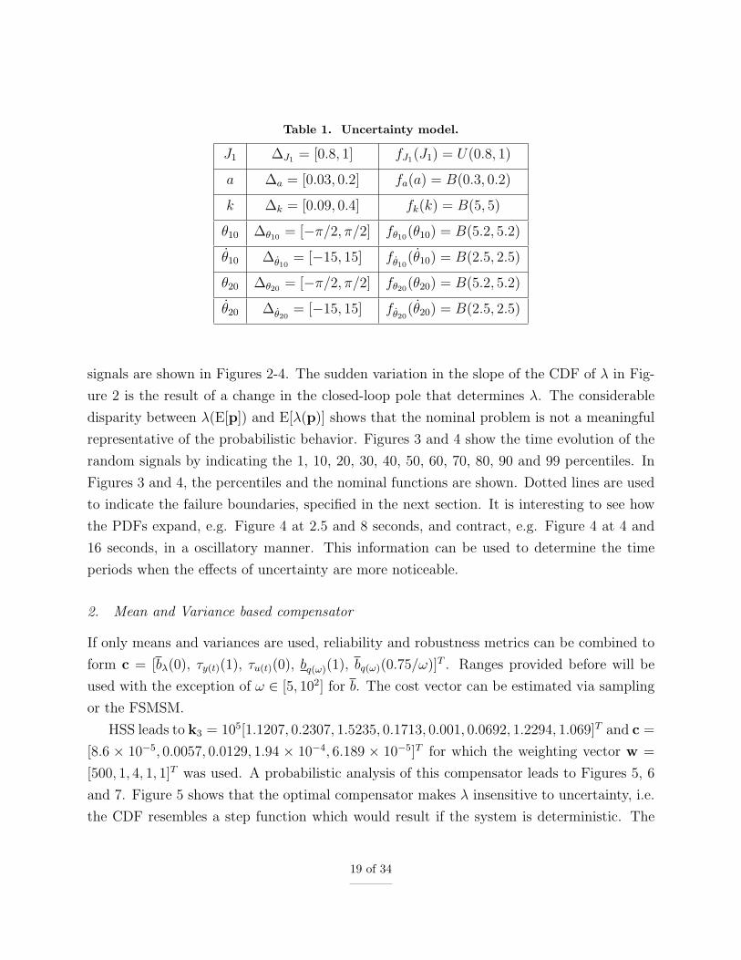
Table 1. Uncertainty model.
J1 ∆J1 = [0.8, 1] fJ1(J1) = U(0.8, 1)
a ∆a = [0.03, 0.2] fa(a) = B(0.3, 0.2)
k ∆k = [0.09, 0.4] fk(k) = B(5, 5)
θ10 ∆θ10 = [−π/2, π/2] fθ10(θ10) = B(5.2, 5.2)
θ10 ∆θ10= [−15, 15] fθ10
(θ10) = B(2.5, 2.5)
θ20 ∆θ20 = [−π/2, π/2] fθ20(θ20) = B(5.2, 5.2)
θ20 ∆θ20= [−15, 15] fθ20
(θ20) = B(2.5, 2.5)
signals are shown in Figures 2-4. The sudden variation in the slope of the CDF of λ in Fig-
ure 2 is the result of a change in the closed-loop pole that determines λ. The considerable
disparity between λ(E[p]) and E[λ(p)] shows that the nominal problem is not a meaningful
representative of the probabilistic behavior. Figures 3 and 4 show the time evolution of the
random signals by indicating the 1, 10, 20, 30, 40, 50, 60, 70, 80, 90 and 99 percentiles. In
Figures 3 and 4, the percentiles and the nominal functions are shown. Dotted lines are used
to indicate the failure boundaries, specified in the next section. It is interesting to see how
the PDFs expand, e.g. Figure 4 at 2.5 and 8 seconds, and contract, e.g. Figure 4 at 4 and
16 seconds, in a oscillatory manner. This information can be used to determine the time
periods when the effects of uncertainty are more noticeable.
2. Mean and Variance based compensator
If only means and variances are used, reliability and robustness metrics can be combined to
form c = [bλ(0), τy(t)(1), τu(t)(0), bq(ω)(1), bq(ω)(0.75/ω)]T . Ranges provided before will be
used with the exception of ω ∈ [5, 102] for b. The cost vector can be estimated via sampling
or the FSMSM.
HSS leads to k3 = 105[1.1207, 0.2307, 1.5235, 0.1713, 0.001, 0.0692, 1.2294, 1.069]T and c =
[8.6 × 10⁻⁵, 0.0057, 0.0129, 1.94 × 10⁻⁴, 6.189 × 10⁻⁵]T for which the weighting vector w =
[500, 1, 4, 1, 1]T was used. A probabilistic analysis of this compensator leads to Figures 5, 6
and 7. Figure 5 shows that the optimal compensator makes λ insensitive to uncertainty, i.e.
the CDF resembles a step function which would result if the system is deterministic. The
19 of 34

Figure 2. CDF of λ for the nominal compensator.
reader must notice that the bound on the stability condition tends to reduce the variability
of λ. This artificially reduces the design space, i.e. there might exist solutions with a better
performance in which large variances in λ occur. This is a consequence of the form of the
bound. This problem has been studied in reference13 using reliability metrics exclusively.
We will refer to this compensator as the reliability compensator. The comparison between
the time responses for the reliability compensator and Figures 6 and 7 show substantial
differences between the two solutions. While the control for the reliability based compensator
intends to keep the process within the strip |u| < 0.5, the mean and variance based solution
intends to concentrate the random process about the target function u = 0. It can be seen
that this is achieved by inducing oscillations about the target function. The reader should
also notice that excursions beyond the failure boundaries in a reliability formulation, are
not penalized according to the severity of the violation. This is in sharp contrast with the
mean and variance formulation. The CPU time for the finer assessment, i.e. the one using
n = 500m p samples, is 77s. For a given number of samples, the estimation of means and
variances is in general more accurate than the estimation of failure probabilities. Small
20 of 34

Figure 3. y(t) for the nominal compensator. A zoom is shown below.
sample sets however, result in larger estimation errors of the moments, which could lead to
the selection of the wrong conditions in Equations (18-19) and (21-22).
Next, the FSMSO method is used. The first and second order derivatives for all the
metrics of interest, i.e. closed-loop poles, output, control and loop transfer function, were
derived analytically. Some of the required expressions are as follows˙x
∂ ˙x
∂2 ˙x
=
A 0 0
∂A A 0
∂2A 2∂A A
x
∂x
∂2x
+
B
∂B
∂2B
u (32)
y
∂y
∂2y
=
C 0 0
∂C C 0
∂2C 2∂C C
x
∂x
∂2x
(33)
where A, B, C, and D were given in Equations (3) and (4), x = [xTc ,xT ]T , ∂[·] indicates a
21 of 34

Figure 4. u(t) for the nominal compensator.
derivative with respect to p(i) excluding initial conditions, and
A∆=
Ac −BcC
BCc A−BDcC
,
∂A =
0 −Bc∂C
∂BCc ∂A−BDc∂C− ∂BDcC
,
∂2A =
0 −Bc∂2C
∂2BCc ∂2A−BDc∂2C− 2∂BDc∂C− ∂2BDcC
,
B∆=[
Bc BDc
]T, ∂B =
[0 ∂BDc
]T, ∂2B =
[0 ∂2BDc
]T,
22 of 34
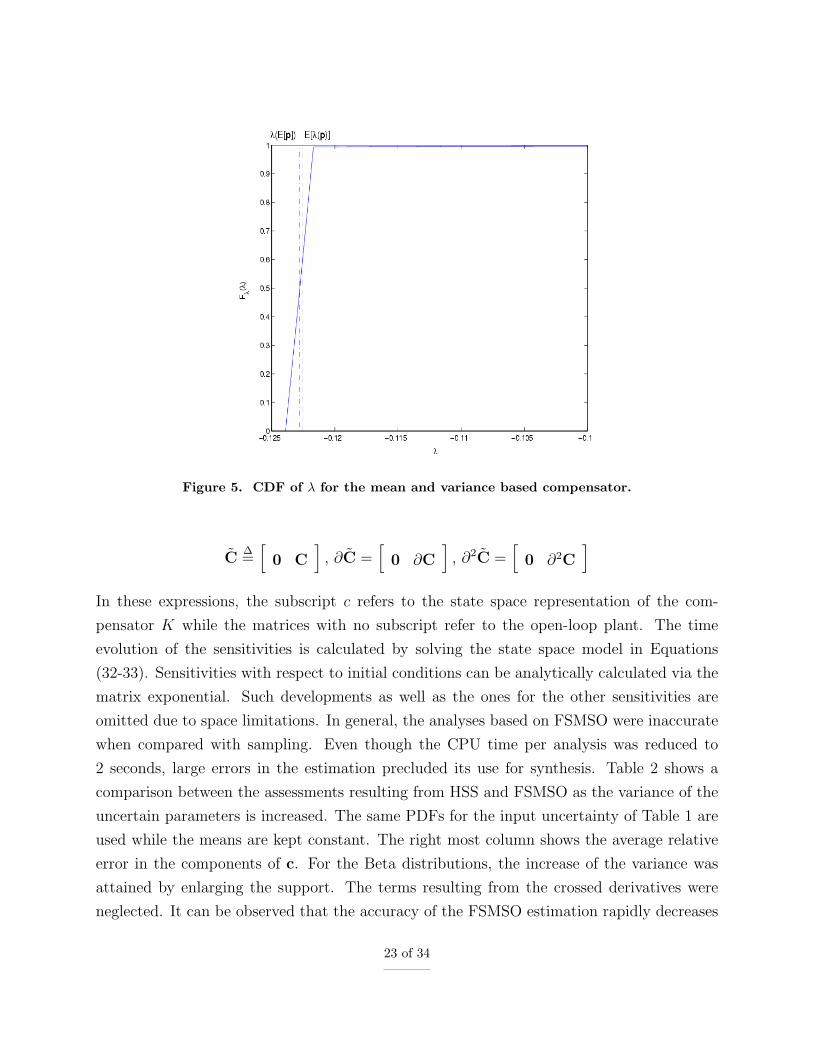
Figure 5. CDF of λ for the mean and variance based compensator.
C∆=[
0 C], ∂C =
[0 ∂C
], ∂2C =
[0 ∂2C
]In these expressions, the subscript c refers to the state space representation of the com-
pensator K while the matrices with no subscript refer to the open-loop plant. The time
evolution of the sensitivities is calculated by solving the state space model in Equations
(32-33). Sensitivities with respect to initial conditions can be analytically calculated via the
matrix exponential. Such developments as well as the ones for the other sensitivities are
omitted due to space limitations. In general, the analyses based on FSMSO were inaccurate
when compared with sampling. Even though the CPU time per analysis was reduced to
2 seconds, large errors in the estimation precluded its use for synthesis. Table 2 shows a
comparison between the assessments resulting from HSS and FSMSO as the variance of the
uncertain parameters is increased. The same PDFs for the input uncertainty of Table 1 are
used while the means are kept constant. The right most column shows the average relative
error in the components of c. For the Beta distributions, the increase of the variance was
attained by enlarging the support. The terms resulting from the crossed derivatives were
neglected. It can be observed that the accuracy of the FSMSO estimation rapidly decreases
23 of 34

Figure 6. y(t) for the mean and variance based compensator. A zoom is shown below.
as fp(p) is less concentrated about its mean. This trait is obvious since large excursions
from E[p] might considerably degrade the accuracy of the Taylor approximation.
The use of reliability bounds introduces unnecessary conservatism into the problem. To
show the reduction in the design space caused by using bλ(0), we have solved this prob-
lem using rλ(0) instead. This practice results in the compensator k4 = 105[0.9082, 0.3590,
1.1773, 0.2372, 0.001, 0.0616, 1.0432, 1.196]T for which c = [1.86×10⁻⁵, 0.0052, 0.0121, 1.845×10⁻⁴, 6.10× 10⁻⁵]T . Figure 8 shows that ∆λ is about 10 times larger than the one in Figure
5. Actually, V[λ] is about 2276 times larger. Large variance values in a formulation using
reliability bounds lead to the penalization of the compensator in spite of its actual improved
performance. The reader should also notice that there is an offset of about 10% between
E[λ] and λ(E[p]). Performance improvements in all the metrics can be seen in Figures 9 and
10.
24 of 34
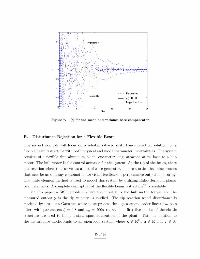
Figure 7. u(t) for the mean and variance base compensator
B. Disturbance Rejection for a Flexible Beam
The second example will focus on a reliability-based disturbance rejection solution for a
flexible beam test article with both physical and modal parameter uncertainties. The system
consists of a flexible thin aluminum blade, one-meter long, attached at its base to a hub
motor. The hub motor is the control actuator for the system. At the tip of the beam, there
is a reaction wheel that serves as a disturbance generator. The test article has nine sensors
that may be used in any combination for either feedback or performance output monitoring.
The finite element method is used to model this system by utilizing Euler-Bernoulli planar
beam elements. A complete description of the flexible beam test article20 is available.
For this paper a SISO problem where the input u is the hub motor torque and the
measured output y is the tip velocity, is studied. The tip reaction wheel disturbance is
modeled by passing a Gaussian white noise process through a second-order linear low-pass
filter, with parameters ζ = 0.8 and ωn = 200π rad/s. The first five modes of the elastic
structure are used to build a state space realization of the plant. This, in addition to
the disturbance model leads to an open-loop system where x ∈ R12, u ∈ R and y ∈ R.
25 of 34

Table 2. Comparison of HSS and FSMSO for k3.
V[p(i)] for Cost vector Average
i = 1, . . . 7 c error
1× 10⁻⁴ cHSS = 10−3[0.000823, 0.0096, 0.5880, 0.0058, 0.0013] 0.3%
cFSMSO = 10−3[0.000827, 0.0095, 0.5880, 0.0058, 0.0001]
1× 10⁻³ cHSS = 10−3[0.00824, 0.0110, 0.6560, 0.0580, 0.0136] 4%
cFSMSO = 10−3[0.00823, 0.0108, 0.7720, 0.0580, 0.0133]
3× 10⁻³ cHSS = 10−3[5.1000, 0.0505, 0.8800, 0.1745, 0.0446] 57%
cFSMSO = 10−3[0.0247, 0.0194, 1.9160, 0.1740, 0.0408]
4× 10⁻³ cHSS = 10−3[32.400, 0.0013, 1.0880, 0.2330, 0.0626] 454%
cFSMSO = 10−3[0.0329, 0.0267, 2.8680, 0.2320, 0.0548]
Figure 8. CDF of λ for a compensator with parameters k4.
The uncertain parameters are the Young’s Modulus E (Pa), the density ρ (Kg/m3) and the
damping ratios of the retained vibration modes. This set leads to p = [E, ρ, ξ1, ξ2, ξ3, ξ4, ξ5]T ,
whose components are assumed independent. The corresponding PDFs are given in Table
26 of 34

Figure 9. y(t) for a compensator with parameters k4. A zoom is shown below.
3. The mean value of the parameters E[p] is set to coincide with the parameters in the
finite element model. These mean values were chosen to match experimental data, while
the supports of the distributions were set according to reasonable ranges of variation. The
shapes of the PDFs were arbitrarily set. Performance requirements on stability and the
output RMS are considered. Full-state feedback with a full-order observer determine the
control structure.
1. Nominal Compensator
As before, a baseline compensator for the nominal plant is designed such that the RMS value
is minimized. The resulting compensator, denoted as d1, leads to yrms = 0.011 m/s. The
propagation of the uncertainty prescribed in Table 3 through the closed loop-system show
that this compensator is robustly unstable with rλ(0) = 0.235.
27 of 34

Figure 10. u(t) for a compensator with parameters k4
2. Reliability-based Compensator
For the sake of comparison, a reliability compensator will be synthesized using the hybrid
method of reference.13 In particular, a shapeable failure domain for the RMS requirement is
assumed. This leads to the cost vector c = [rλ(0), ryrms(e) + γyrms]T , where e ∈ [0, 0.05] and
γyrms = e. The selected control structure makes the feedback gain G, the observer gain L,
and the RMS failure boundary e, the design variables. Recall that the separation principle
does not hold. The resulting closed-loop dynamics is given by Equations (3) and (4). Notice
that although the observer is deterministic, all the closed-loop poles are random.
The synthesis approach with w = [20, 1]T leads to a compensator with parameters d2,
for which rλ(0) = 0, e = 0.0139 m/s, ryrms(e) = 3.6 × 10⁻³ and c = [0, 3.6 × 10⁻³]T . The
probabilistic analysis of d2 leads to Figures 11-12. Figure 11 shows that the random variable
yrms is moved toward zero, by virtue of the non-fixed failure boundary. In addition, Figure
12 shows Bode magnitude plots of the disturbance to output transfer function, namely Tzy.
Notice that differences in the low-frequency portion of the diagram have a bigger impact
on the RMS value. In addition, considerable variability in the closed-loop Bode magnitude
28 of 34

Table 3. Uncertainty model.
E ∆E = 1010[5.226, 7.839] fE(E) = B(5, 5)
ρ ∆ρ = [2280, 3420] fρ(ρ) = B(3, 3)
ξ1 ∆ξ1 = [0.08, 0.12] fξ1(ξ1) = B(2, 2)
ξ2 ∆ξ2 = [0.0252, 0.0378] fξ2(ξ2) = B(2, 2)
ξ3 ∆ξ3 = [0.02, 0.03] fξ3(ξ3) = B(2, 2)
ξ4 ∆ξ4 = [0.0304, 0.0456] fξ4(ξ4) = B(2, 2)
ξ5 ∆ξ3 = [0.02, 0.03] fξ5(ξ5) = B(2, 2)
plot as well as a significant reduction in the damping of the first mode are attained near 20
rad/s. It is interesting to notice that even though d2 leads to a robustly stable closed-loop
system in Equation (3), the full-state feedback subsystem A1,1 and the full-order observer
subsystem A2,2 have a non-zero probability of instability. This indicates that the Separation
Principle artificially reduces the design space once uncertainty is present.
Figure 11. PDFs for the reliability based and the robustness based compensators.
29 of 34

Figure 12. Bode diagrams of Tzy for d2.
3. Mixed Compensator
Lets take c = [rλ(0), τyrms(0)]T , where the hybrid approach of reference13 will be used for the
stability metric and HSS for the RMS metric. The synthesis algorithm leads to d3, for which
c = [0, 1.34 × 10⁻⁴]T . This compensator leads to the dashed line in Figure 11. Comparing
both solutions, we see that while the PDF corresponding to the reliability-based compensator
has less probability of exceeding the boundary value of e = 0.0139 m/s, the robustness-based
compensator leads to a PDF which is much more concentrated toward the ideal value of zero.
This clearly shows that the conceptual differences between the two formulations. Since there
is no conservatism in the selection of the nominal plant, i.e., G(E[p]) is not the most difficult
plant to control, yrms = 0.011 m/s does not necessarily bound the supports of the PDFs. This
can be observed in Figure 11, where the support corresponding to d3 contains yrms = 0.011
m/s.
30 of 34

4. Mean and Variance based Compensator
For this case we assume c = [bλ(0), τyrms(0)]T , where the FSMSO method will be used
to estimate both indexes. In contrast to the satellite attitude example, the accuracy of
the FSMSO method made it suitable for synthesis. Analytical sensitivities were used in
the moments approximations. For instance, the sensitivities of the closed-loop poles that
determine λ are given by
Avj = sjvj
∂sj = zTj ∂Avj
∂2sj = zTj
[∂2A + (∂A− ∂sjI)(sjI− A)−1∂A + ∂A(sjI− A)−1(∂A− ∂sjI)
]vj
where zj is the jth eigenvector of AT , the right and left eigenvalues are normalized, i.e.
zTj vj = 1, and and non-repeated poles are assumed. See the work of Burchett and Costello21
for a review on the subject. Derivatives of the output covariance are given by
∂yrms ={
diag[C∂QCT + 2∂CQCT
]}1/2
∂2yrms ={
diag[C∂2QCT + 4∂C∂QCT + 2∂2CQCT + 2∂C∂Q∂CT
]}1/2
where the derivatives of the state covariance are given by the solution to the set of Lyapunov
equations
A∂Q + ∂QAT + ∂AQ + Q∂AT + ∂BSBT + BS∂BT = 0
A∂2Q + ∂2QAT + 2∂A∂Q + 2∂Q∂AT + ∂2A∂Q+
∂Q∂2AT + 2∂BS∂BT + ∂2BSBT + BS∂2BT = 0
The synthesis algorithm leads to d4, for which c = [5.33× 10⁻⁶, 1.33× 10⁻⁴]T . The resulting
PDF for the RMS is indistinguishable from the one shown in Figure 11 even though the
compensators are different. The CDFs of λ for d3 and d4 are superimposed in Figure
13. As before, the tendency of the formulation of making λ as deterministic as possible is
31 of 34

apparent. Notice however, that the CPU time required for the analysis of d3 is 421 s while
the one for d4 is 1.22 s. On the other hand, the analysis of d4 via HSS takes 64 s. This
exemplifies substantial savings in CPU time which result from using the FSMSO method.
In this example, those savings justify the labor required to compute analytical derivatives.
The reader must recall, however, that the same method led to inaccurate estimations for the
satellite example.
Figure 13. CDFs of λ for d3 and d4.
VIII. Conclusions
This paper proposes a control synthesis methodology for systems with probabilistic un-
certainty. Synthesis is performed by solving a multi-objective optimization problem which
combines requirements of stability and performance in time- and frequency-domains. In this
study, reliability- and robustness- based formulations are proposed and several numerical
methods for estimation are examined. In a reliability formulation, the probability of violat-
ing design requirements is minimized while admissible domains are contracted toward regions
with an improved performance. In a robustness-based formulation, a random metric that
32 of 34
measures the concentration of the random variable/process about a target scalar/function is
minimized. These two formulations lead to compensators with distinctive characteristics. In
addition, metrics that bound the reliability metrics proposed, whose estimation only requires
of means and variances, are also derived and used for control design.
Some of the fundamental differences between the proposed strategy and conventional ro-
bust control methods are: (i) unnecessary conservatism is eliminated since there is not need
for convex supports/sets, (ii) the most likely plants are favored during synthesis allowing for
probabilistic robust optimality, (iii) the trade off between robust stability and robust per-
formance can be explored numerically, (iv) the uncertainty set, which could be unbounded,
is closely related to parameters with clear physical meaning and (v) compensators with im-
proved robust characteristics for a given control structure can be designed, e.g. one can
search for a PID controller with best robust characteristics. Examples of attitude control of
a simple satellite model and disturbance rejection of a flexible beam are used to elucidate
the nature of the problem at hand and to demonstrate the methodology.
References
1Crespo, L. G., “Optimal performance, robustness and reliability based designs of systems with struc-tured uncertainty,” Proceedings of American Control Conference, Vol. 5, Denver, CO USA, June 2003, pp.4219–4224.
2Laughlin, D. L., Jordan, K. G., and Morari, M., “Internal model control and process uncertainty -mapping uncertainty regions for SISO controller design,” International Journal of Control , Vol. 44, No. 6,December 1986, pp. 1675–1698.
3Weinmann, A., Uncertain Models and Robust Control , Springer-Verlag, New York, NY USA, 1991.4Zhou, K. and Doyle, J. C., Essentials of Robust Control , Prentice Hall, Upper saddle, New Jersey,
1998.5Marrison, C. and Stengel, R., “Design of Robust Control Systems for a Hypersonic Aircraft,” Journal
of Guidance, Control, and Dynamics, Vol. 21, January-February 1998, pp. 58–63.6Wang, Q. and Stengel, R. F., “Robust Nonlinear Control of a Hypersonic Aircraft,” Journal of Guid-
ance, Control, and Dynamics, Vol. 23, No. 4, July-August 2000, pp. 577–585.7Wang, Q. and Stengel, R. F., “Searching for Robust Minimal-Order Compensators,” Journal of Dy-
namic Systems, Measurement and Control , Vol. 123, June 2001, pp. 233–236.8Calafiore, G., Dabbene, F., and Tempo, R., “Randomized Algorithms for Probabilistic Robustness
with Real and Complex Structured Uncertainty,” IEEE Transactions on Automatic Control , Vol. 45, No. 12,December 2000, pp. 2218–2235.
33 of 34

9Polyak, B. and Tempo, R., “Probabilistic robust design with linear quadratic regulators,” Systems andControl Letters, Vol. 43, 2001, pp. 343–353.
10Lagoa, C. M., Li, X., and Sznaier, M., “On the Design of Robust Controllers for Arbitrary UncertaintyStructures,” IEEE Transactions on Automatic Control , Vol. 48, No. 11, November 2003, pp. 2061–2065.
11Spencer, B. F., Sain, M. K., Won, C.-H., Kaspari, D. C., and Sain, P. M., “Reliability-based measuresof structural control robustness,” Structural Safety , Vol. 15, 1994, pp. 111–129.
12Rackwitz, R., “Reliability analysis, a review and some perspectives,” Structural Safety , Vol. 23, 2001,pp. 365–395.
13Crespo, L. G. and Kenny, S. P., “Reliability-based control design for uncertain systems,” AIAA Journalof Guidance, Control, and Dynamics, Vol. 28, No. 4, 2005.
14Wang, Q. and Stengel, R. F., “Robust control of nonlinear systems with parametric uncertainty,”Automatica, Vol. 38, 2002, pp. 1591–1599.
15Crespo, L. G., “Probabilistic formulations to robust optimal control,” 45th AIAA Structures, StructuralDynamics and Materials Conference, Palm Springs, CA USA, April 2005, pp. 1–21, AIAA Paper No. 2004-1667.
16Skogestad, S. and Postlethwaite, I., Multivariable feedback control , John Wiley and Sons, Chichester,England, 1996.
17Hokayem, P., Abdallah, C., and Dorato, P., “Quasi-Monte Carlo Methods in Robust Control Design,”IEEE Conference on Decision and Control , Maui, HA USA, December 2003, pp. 2435–2440.
18Kalagnanam, J. R. and Diwekar, U. M., “An Efficient Sampling Technique for Off-line Quality Con-trol,” Technometrics, Vol. 39, No. 3, August 1997, pp. 308–319.
19Diwekar, U. M. and Kalagnanam, J. R., “Efficient Sampling Technique for Optimization under Uncer-tainty,” American Institute of Chemical Engineering Journal , Vol. 43, No. 2, February 1997, pp. 440–447.
20Kenny, S. P., Optimal rejection of nonstationary narrowband disturbances for flexible systems, Ph.D.thesis, Massachusetts Institute of Technology, Cambridge, MA USA, February, 2002.
21Burchett, B. and Costello, M., “QR-Based Algorithm for Eigenvalue Derivatives,” AIAA Journal ,Vol. 11, No. 40, November 2002, pp. 2319–2322.
34 of 34
Top Related