


Languages
Pages
Legal


Munich Personal RePEc Archive
A Dynamic Inflation Hedging Trading
Strategy Using a CPPI
Fulli-Lemaire, Nicolas
University of Paris II, Crédit Agricole SA
2 January 2012
Online at https://mpra.ub.uni-muenchen.de/43620/
MPRA Paper No. 43620, posted 08 Jan 2013 13:58 UTC
1
A Dynamic Inflation Hedging Trading Strategy using a CPPI
Nicolas Fulli-Lemaire1
Amundi Paris II University
Fourth Version: 04/01/2013
Published in the Journal of Finance & Risk Perspective: December 2012, Volume 1 (Issue2).
Abstract
This article tries to solve the portfolio inflation hedging problem
by introducing a new class of dynamic trading strategies derived
from classic portfolio insurance techniques adapted to the real
world. These strategies aim at yielding higher returns on a risk-
adjusted basis than regular inflation hedging portfolio allocation
while achieving a lower cost than comparable option–based
guaranteed real value strategies.
Keywords: ALM, Inflation Hedging, Portfolio Insurance, CPPI.
JEL classification: C58, C63, E31, E43, E52 ,G12, G2, Q0.
1 This document presents the ideas and the views of the author only and does not reflect Amundi’s opinion in any way. It does not constitute an investment advice and is for information purpose only.

2
Plan
Introduction .................................................................................................................................... 3
1. Inflation Hedging and Portfolio Insurance ................................................................................ 4
1.1. Motivations for seeking alternative hedges, a review of the existing literature .................... 4
1.2. Adapting Portfolio Insurance techniques to the real world .................................................... 6
2. Theoretical construction of the DIHTS ...................................................................................... 9
2.1. The DIHTS as an alternative strategy ...................................................................................... 9
2.2. Optimal allocation of the diversified portfolio ...................................................................... 13
3. Empirical estimations of the performance of the strategy ...................................................... 14
3.1. Methodology and data sources ............................................................................................. 14
3.2. Historical Backtesting results ................................................................................................ 16
4. Block Bootstrapping based evaluation of the DIHTS ............................................................... 17
4.1. Principle ................................................................................................................................. 17
4.2. Results ................................................................................................................................... 19
Conclusion .................................................................................................................................... 21
Appendix ....................................................................................................................................... 23
A. Historical Simulation Results ..................................................................................................... 23
B. Bootstrapped Simulation Results .............................................................................................. 31
References .................................................................................................................................... 37
List of Figures ................................................................................................................................ 39
List of Tables ................................................................................................................................. 39

3
Introduction
The demand for inflation hedges from pension funds has spurred the academic
literature on optimal portfolio allocation and investment strategies for durations up to several
decades. These types of long haul strategies are designed to match future liabilities that must
be provisioned but that do not require specifically that the mark to market value of their
investments matches that of their liabilities in the short run. In this paper, we set ourselves in
the different context of commercial banks that need to hedge their inflation liabilities arousing
from retail products such as guaranteed power purchasing saving accounts, term deposits, or
even asset management structured products. All of these guarantees are immediately effective
and their duration rarely exceeds a decade. Moreover, a constant access to liquidity is required
for these open funds which can face partial or total redemption any time during their lifetime.
This new framework requires the construction of an investment strategy that must
have a positive mark to market real value at its inception and throughout its life. Also,
because of the constraints resting on the inflation linked market we expose in our first part, we
seek to develop a strategy that would be purely nominal, that is entirely free of inflation
indexed products which are costly and therefore reduce the potential real return. After
summarizing the possible alternative inflation hedges in a second part, we explore the
feasibility of adapting portfolio insurance techniques to the inflation hedging context in order
to honor our guarantees while exploiting the inflation hedging potential of alternative asset
classes. We seek to avoid the use of derivative instruments which costs can be prohibitive
considering the scale of the liabilities. Combining all the above-mentioned points, we
introduce our Dynamic Inflation Hedging Trading Strategy (DIHTS) and backtest its
performance on a long US historical dataset which we use both for historic simulation and
bootstrapped simulation.
4
1. Inflation Hedging and Portfolio Insurance
1.1. Motivations for seeking alternative hedges, a review of the existing
literature
Corporations which are structurally exposed to inflation would most naturally like to
hedge their liabilities by the purchase of inflation linked financial assets, or by entering in
derivative contracts which would outsource the risk. But these two natural solutions rely on an
insufficiently deep and insufficiently liquid market for the first one and is excessively costly
for the second one as a result of an unbalanced market:
On the demand side of the inflation financial market, the need for inflation protected
investments is spurred by four main drivers which are pension funds because of their inflation
liabilities arousing from explicit power purchasing guaranteed pensions, retail asset managers
providing inflation protected funds, insurance companies hedging their residual inflation
liabilities and, mostly in continental Europe, commercial banks exposed to state guaranteed
inflation indexed saving accounts. The bulks of those liabilities have long to vey long
durations and amount to the equivalent of hundreds of billions of Euros. On the supply side
of the market for inflation-linked bonds, there is a very limited pool of issuers which is
comprised mostly of sovereign or quasi-sovereign entities. There are very few corporate
issuers of inflation linked bonds as there are very few corporations that have a structural long
net exposure to inflation to the exception of maybe utilities engaging in Public-Private-
Partnerships or real-estate leasers which tariffs are periodically adjusted on an inflation basis
by law or contract. And even in those cases, it is not obvious that those companies have an
interest in financing their operations on an inflation-linked basis which in nominal term is a
floating rate. In fact, very few choose to. This limited pool of issuers is subject to changing
budget policies, issuance strategies and current deficits which result in a fluctuating primary
supply. Moreover, most of the buyers in the primary market acquire those assets on a hold to
maturity basis or for immediate repo, rendering the secondary market relatively more illiquid
than the one of their nominal counterparts, as is evidenced in the working paper(D'Amico,
Kim et Wei 2009).
The derivative market for inflation is characterized by relatively high transaction costs
as a result of shallow depth at reasonable price. Since on the one hand the sellers of those
instruments will either have to hedge their trading books on the shallow and illiquid primary
inflation market or assume the full inflation directional risk as a result of cross-hedging on
nominal assets but on the other hand face a huge demand, the required premiums are very
high. There has been since the mid 2000 a liquid market for exchange traded inflation swaps
which has enabled to price inflation breakeven rates. There is to this day no liquid exchange
traded market for inflation options as most of the deals are done in an Over-The-Counter
basis. If the domestic supply of inflation linked instruments is not sufficient to meet the
demand, as it is often the case, there is little international diversification can do as inflation is
mostly a domestic variable which correlation to other foreign equivalents can be fickle, even
in the case of monetary unions or currency pegs where foreign exchange is not an issue like in
the Euro-Area. The recent Euro-area sovereign crisis has made this point all the more acute.

5
This gap between supply and demand in the inflation financial market has spurred the
interest in alternative inflation hedging techniques that could solve the depth, cost and
liquidity issues that have plagued the inflation financial market. Academic literature dating
back from as far as the seventies has explored the use of a portfolio of real investments as an
inflation hedge. Various asset classes such as equities (Z. Bodie 1976), commodities (Z.
Bodie 1983), real estate (Rubens, Bond et Webb 2009), REITS (Park, Mullineaux et Chew
1990), and more recently dividend indices(Barclays Capital Research 2008) have been
examined as potential real hedges to inflation. Even exotic assets such as forest assets
(Washburn et Binkley 1993) and farmland (Newell et Lincoln 2009) just to mention two of
them have also been explored but offer very limited interest with respect to the added
complexity their investment requires.
The first emission of a long term CPI linked bond by a private US financial institution
in the late eighties has led to a string of papers starting with (Z. Bodie 1990) which aimed at
finding the optimal strategic asset mix these new assets enabled. Similarly, the first issuance
by the United States treasury of inflation protected securities in 1997, following the first
issuance by the British treasury of inflation linked gilts in 1981 have generated a renewal of
interest in their role as inflation risk mitigation and diversification assets. The latest of which
is the(Brière et Signori 2010) paper. These studies are of limited help for the purpose of this
work as they still rely for a significant fraction of their investment strategies on inflation
linked assets, which we are precisely trying to avoid doing. They nonetheless offer a first
alternative to fully inflation protected investments, and therefore offer a potentially higher
degree of returns, at the cost of a more hazardous hedging method.
Another stream of academic literature has focused on the optimal allocation for
inflation hedging portfolios using only nominal assets and using various approaches to
determine the optimal allocation like the recent (Amenc, Martellini et Ziemann 2009) paper
which devised a global unconstrained nominal inflation hedging portfolio that would use a
Vector Error Correcting Model to determine the optimal ex-ante allocation of the various
potential inflation hedging asset classes mentioned before. This kind of strategy would solve
the availability problem of the inflation linked assets, but would fail to bring any kind of
guaranteed value to the portfolio, be it in real or nominal terms, and because of that, fails to
meet our Asset Liability Management (ALM) constraints. In fact, the hedging potential of all
the above-mentioned asset classes has proved to be horizon sensitive and dependent on the
macroeconomic context. (Attié et Roache 2009) have studied the time sensitivity of the
inflation hedging potential of various asset classes and have shown in particular that some
asset classes like commodities react better to unexpected inflation shocks than others, like
most obviously nominal bond. More generally, the inflation betas has also proved to be
unstable over time and can exhibit strong local decorrelations, rendering the inflation hedging
exercise risky considering for example that the volatility of most of these asset classes is far
superior to that of the Consumer Price Index we are precisely trying to hedge.
Using an error correction framework to optimize the portfolio allocation might have
solved part of the problem by incorporating into the model those dynamics in asset price
levels and returns that might otherwise have been overlooked as outliers by more general

6
VAR models, but these classes of models are tricky to calibrate and would most probably
result in statistically insignificant estimations, and accordingly, wrong allocations. Moreover,
they would also most probably fail to detect in a timely manner small macroeconomic regime
changes that could have a lastingly impact on the structure of the inflation betas. This might in
turn jeopardize the overall inflation hedging potential of the portfolio if for example one of
the invested assets suffered a significant fall in value as none of them has a guaranteed value
at maturity like a bond, credit risk apart. Overall, this type of strategies would still fall short of
a totally guaranteed value for the portfolio as would be the case with a real zero coupon bond.
1.2. Adapting Portfolio Insurance techniques to the real world
The limitations in term of guaranteed terminal value for the classic Markowitz
approach to optimal portfolio selection based on the benefit of diversification have motivated
the quest for portfolio insurance strategies in the seventies (Leland, Who Should Buy
Portfolio Insurance? 1980). In purely nominal terms, the optimal tradeoff between the
enhanced returns on risky assets and the low returns on assumed risk-free nominal bonds is
known as the “two fund theorem”. The optimization can also be further constrained by
incorporating guaranteed nominal-value-at-maturity characteristics. Doing so yields the so
called Dynamic Portfolio Insurance Strategies (Perold et Sharpe 1988) which includes: Buy
and Hold, Constant Mix, Constant Proportion and Option Based Portfolio Insurance. But can
such guaranteed-values-at-maturity strategies be transposed to the real world?
The simplest solution would be to mimic a two fund strategy in the real world: it
would be implemented using a real risk free zero coupon bond and either a diversified
portfolio of real assets or a call on the real performance of a basket of assets. The call option
could also be either bought or replicated using an adaptation of the ideas exposed in(Leland et
Rubinstein, Replicating Options with Positions in Stocks and Cash 1981). Such strategies
would unfortunately be highly intensive in inflation indexed products use and would therefore
not solve our availability problem, without even taking into account the low real returns these
strategies would probably yield.
Using a call option on nominal assets, as opposed to real assets, would only partly
solve the problem as the risk-free part is either made of zero coupon bonds which are
available in limited supply or synthetic bonds made of nominal zero coupon bonds combined
with a zero coupon inflation index swap which have greater supply but very low real returns.
It could also be envisaged to combine a risk free zero coupon nominal bond and an out of the
money call option on inflation. It would almost exactly be a replication of an inflation index
bond as we will explain in the next subsection.
A last possibility would involve the transposition of the CPPI technique of (Black et
Jones 1987) in the real world by using the above mentioned techniques to dynamically
manage a cushion of inflation indexed bond and a portfolio of real return yielding assets. As
was mentioned before, this strategy would still rely on indexed assets. The inflation hedging
portfolio insurance problem would therefore be solved without investing in inflation linked

7
assets or derivatives if it were possible to generate a portfolio that could mimic the cash-flows
of an inflation-linked-bond as we will try to prove in the next subsection.
To sum up, any real portfolio insurance strategy would involve a capital guaranteeing
part and a real performance seeking investment made of a diversified portfolio or a derivative
and without explicit capital guarantees at maturity. Depending on the strategy used, the
guaranteed capital part would either have a real guarantee embedded, or simply a nominal
guarantee which would have to be complemented by a real guarantee attained to the detriment
of the performance seeking part.
Trying to do without the IL instruments, we want to replicate the cash flow of an ILB
with a Fisher Hypothesis. This replication can be achieved using an adapted OBPI technique
as mentioned in the previous subsection and the theoretical justification is provided below:
Replicating the cash flows of an ILB is equivalent to fully hedging a nominal portfolio on a
real basis. To do so, we need to invest a fraction α of the notional of the portfolio N in a zero
coupon nominal bond of rate τ , and buy a cap to hedge the residual risk. Out of simplicity,
N is assumed hereunder to have a unit value. Using the Fisher framework (Fisher 1907), we
can decompose the nominal bond’s rate into a real rate τ , , an inflation anticipation π ,
and an inflation premium p π , : 1 τ , 1 τ , 1 π , 1 p π ,
The nominal bond’s allocation α should then be defined such that its inflation components
equalize the ILB’s one. We obtain the following equation by ignoring the cross product :
α 1 π , 1 p π , 1 π , ⇒ α 11 p π ,
We are left with a residual amount 1 α out of which we can buy the option without
shorting.
Let π , be the realized inflation between 0 and T, let S be the initial spot rate for inflation
equal to π , under the rational expectation hypothesis and let c , ; be the cap premia
of strike K and maturity T at 0 be expressed as a percentage of the notional.
By a simple absence of arbitrage opportunity hypothesis, we can rule out ITM strikes: ∄K S suchthatc , ; 1 α
When short selling is also prohibited, we have strikes that are OTM or at best ATM. This
would constitute a partial hedge in which we would remain at risk on the spread: ResidualRisk K S , ifS ∈ S , K0otherwise

8
If we can borrow at rate τ , , we can then fully hedge our portfolio. Ignoring the cross
products, we obtain under those assumptions the nominal return N : N ατ , π , π , π , 1 α c , ; 1 τ ,
The real returnR is thus: R ατ , π , π , π , 1 α c , ; 1 τ , π ,
Applying the cap-floor parity, we have : π , π , π , π , π , π ,
Which gives us the following result for the real rate: R ατ , π , π , 1 α c , ; 1 τ ,
Nota bene: This return is not necessarily positive.
In fact, since call options on inflation are not liquid exchange-traded instruments but
OTC products, there is a high probability that the call premium would be sufficiently high to
render the real return of the strategy very low at best if not negative at worst. This is not
inconsistent with empirical observations that have been made on real bonds: some TIPS
issuances in 2010 have had negative real rates.
The replication of the ILB cash flows by a combination of a nominal bond and a call
option on inflation still fails to fully satisfy our objective of getting rid of the dependency on
the inflation financial market because of the call option. To relax this constraint, it might be
possible to manage the option in a gamma trading strategy without having to outrightly buy
the derivative. The obvious challenge to overcome is that the natural underlying of the call
option is an inflation indexed security, which brings us back to our previous hurdle. To
overcome this latest challenge, it could be possible to envisage a cross-hedging trading
strategy to gamma hedge the call on purely nominal underlings as will be exposed in the next
subsection. (Brennan et Xia 2002) proposed a purely nominal static strategy that would both
replicate a zero coupon real bond and invest the residual fraction of the portfolio in equity
while taking into account the horizon and the risk aversion of the investor in a finite horizon
utility maximization framework. We would like to extend the scope of this work to dynamic
allocation.

9
2. Theoretical construction of the DIHTS
2.1. The DIHTS as an alternative strategy
To achieve this inflation hedging portfolio insurance, we would like to capitalize on
the popular CPPI strategy to build a dynamic trading algorithm that would be virtually free of
inflation linked products and derivatives, but still offer a nominal and a real value-at-maturity
guarantee: we propose a strategy which we will call the Dynamic Inflation Hedging Trading
Strategy (DIHTS).
The risk-free part of the DIHTS portfolio would be invested in nominal zero coupon
bonds which maturity matches that of our target maturity. The ideal asset for our strategy
would be a floating rate long duration bond but since too few corporate or sovereign issuers
favor this type of product, we cannot base a credible strategy relying on them. We could swap
the fixed rate of the bond for a floating rate with a Constant Maturity Swap (CMS) as this
type of fixed income derivative does not suffer for the limited supply and its cost implications
like inflation indexed ones as it boasts a much boarder base of possible underlings in the
interest rate market. Also, contrary to the inflation financial market, there are players in the
market which are naturally exposed to floating rate and who wish to hedge away this risk by
entering in the opposite side of a CMS transaction, therefore enhancing liquidity and driving
the cost down for such products. But, we have to accept bearing huge costs if the portfolio is
readjusted as long rates move up or have to forfeit the capital guarantee at maturity by
synthesizing the CMS by rolling positions on long duration bonds. Either which of these
options are hardly sustainable.
Be it a fixed or a floating rate bond, a nominal security does offer only a limited
inflation hedging potential: even if the Fisher framework exposed previously can let us hope
that an increase in expected future inflation will drive rates up, the economic theory tells us
that the Mundell-Tobin effect will reduce the Fisher effect and therefore reduce the inflation
hedging potential of nominal floating rate asset, which, though not capped as in fixed rate
assets, will still fail to hedge entirely the inflation risk. The residual part of this risk has to be
hedged away by incorporating the real guarantee in the diversified part of the portfolio which
is made up of potential inflation hedging asset classes which we will limit to three: equities,
commodities and REITS. Subsequent work could exploit a finer distinction between
commodities by dividing them in for example four sub-classes: soft, industrial metals,
precious metals and energy. The tactical allocation of the portfolio will be made according to
a systematic algorithm which doesn’t allow for asset manager input as a first step. Eventually
a more complex asset allocation algorithm could be added. We assume, as in the portfolio
insurance literature, that there is no credit risk in either one of the fixed income assets we
hold. The value at maturity of these assets is therefore their full notional value. We do not
assume any outright hypothesis on the guaranteed value-at-maturity for the diversification
asset, but as in any CPPI strategy, a maximum resilience has to be set at a desired level which
we will denote . The parameter could be set specifically for each asset class, but we will
assume only a single one for simplicity.

10
If we add a martingale hypothesis for the price process of the other asset classes:
This “limited liability” assumption becomes equivalent to a value-at-maturity hypothesis for
the diversified portfolio which we can write for being the guaranteed value at maturity: ∙
By further assuming that expected inflation can be obtained by the use of BEIs derived from
ZCIIS, we can compute the initial fixed income fraction of the DIHTS which we will
denote .
Let , be the realized inflation between t and t+ , and let , be the expected inflation
between t and t+ at time . We have:
, , ,
Let’s further assume that: ∀ , , 0
We then assume that:
, ,
This assumption simplifies the problem of the computation of the inflation expectation in a
rational anticipation framework: since in the Fisher framework we have: 1 , 1 , 1 ,
The above assumption is equivalent to considering that the risk premiums are nil, which is a
prudent hypothesis since they are non-negative: we therefore never underestimate the inflation
risk. This hypothesis will have a further justification when we’ll discuss the definition of the
DIHTS’ floor.
The use of DIHTS in an ALM strategy as it is presented here is better fitting for long
term investors who wish to diversify away from zero-coupons inflation derivatives yielding
back in bullet both the inflated principal and the real performance at maturity. It would be
better fitting for retail oriented asset managers or pension funds. Investors wishing to
diversify away from year-on-year type of inflation derivatives would rather use a strategy
which cash flow profile still matches that of their liabilities which could for example require
that the instrument pays the accrued inflation on the notional, and eventually a real coupon, on
a yearly basis such that the instrument is at a yearly real par. Such strategies would benefit
from an enhanced version of DIHTS using couponed bonds and eventually CMS-like fixed
income derivatives in overlay to replicate our targeted benchmark instrument while still

11
exploiting the same general principal as for the simpler strategy presented here. Henceforth,
we will focus only on bullet repaying strategies since the marking-to-market allows us to
theoretically adjust the notional of the fund at a current value, therefore without risking
incurring a loss in case of partial or total redemption from the fund.
As previously defined, denotes the fraction of the fund invested in risk free nominal assets.
Let , 1 be the initial global allocation of the DIHTS and NPV denotes the net
present value of the two fractions. All rates from now on are given in annual rate. At
inception: 1 α ∙ μ α 1 π ,1 τ ,
We therefore have
α 1 π ,1 τ , μ 11 μ
Let Α , represent the ZC zero coupon bonds fraction of equivalent tenor (T-t), invested at
time t and maturing at time T (for a ZCNB, only the nominal at maturity counts):
Let NAV represent the NAV of the zero coupon part, we have:
NAV Α ,1 τ ,
Let be the weights of the ex-ante optimal allocation of the diversified portfolio, let Ω be
the vector of the value of the assets of the portfolio and let be the price vector of the
selected asset classes. From now on, the star will denote the post optimization value of the
parameter. We have at inception:
∗ Ω∗1
1 ∗ ∙ We then define as:
Ω∗ ′ ∙
And as: 1 , 1 ,1 ,

12
For any 0, we define the net asset value of the strategy :
Before any reallocation we have:
Let be the implicitly guaranteed net asset value of the strategy taking into account the
loss resilience parameter : ∙
The strategy remains viable as long as 0. If the floor is breached, the fund is closed
before the maturity or a zero coupon inflation hedging security would have to be bought at a
loss.
A global reallocation is necessary if 0 and in which case, we have to add a new
trench of ZCNB such that: ∗ argmin 0
In case we have: 0 0weset 0
Since the expected returns on the diversified part of the portfolio are potentially higher than
those on the fixed income part, we set at the lowest possible value that verifies 0.
In order not to reallocate constantly the global parameter at the slightest market movement,
we set a tolerance parameter under which no global reallocation is done: ∗ | | 0 0
Obviously, any global reallocation would trigger a reallocation of the diversified portfolio
weights. It is a sufficient but not necessary condition as it may be more optimal to do so more
frequently as we will expose in the next subsection.
The breaching of the DIHTS’ floor is obtained when it is not possible to reallocate the
global parameter such that the guaranteed net asset value becomes positive: ∀ 0, 0
If such an event were to occur, the diversified portfolio would already have been
entirely liquidated and the remaining net asset value could as before be used to buy a string of
ZCIIS to insure the real guarantee at maturity of the portfolio. The gap risk and the liquidation
cost would probably result in a negative real return. Gap risk apart, the downside risk would

13
be curtailed by the fact that we had taken ZCIIS BEIs when computing the NAV and not
directly the expected inflation which would have been lower.
2.2. Optimal allocation of the diversified portfolio
The diversification portfolio is allocated in order to hedge both the residual expected
inflation and the unexpected inflation, while also yielding the real excess return that is
targeted. Once the global allocation parameter is set, we can compute the residual expected
inflation and eventually set a targeted real excess return. According to our hypothesis, we
have no input regarding the value of the unexpected inflation which ex-ante conditional
expectation is nil.
Out of all the possible portfolio optimization criteria, we will limit ourselves to
envisaging allocating the diversified portfolio according to three criteria: a Constant Weight
scheme (CW), a minimum-variance (MV) and an Information Ratio (IR). We introduce the
following definitions: Let be the targeted real return scalar, be the realized return vector
over the period k for the different asset classes and Σ be the variance-covariance matrix of the
return vector at time t. Let be a portfolio allocation at time t and ∗ be the optimal one
according to the X criteria used. Let be the realized inflation over the k period, be the
expected inflation over the k period at time t and be the nominal return on the fixed-
income investment.
The MV optimization criterion is defined by the following loss function at time t: , , , , , Σ ∙ Σ ∙
We therefore obtain the optimal portfolio according to the MV criterion by minimizing L: ∗ argmin , , , Σ
The IR optimization criterion is defined such that: , , , , , Σ , ∙ , 11 , ∙∙ Σ ∙
We therefore obtain the optimal portfolio according to the IR criterion by maximizing the IR: ∗ argmax , , , , , Σ ,
The first criterion required at least the estimation of the variance-covariance matrix of
the investable assets and the second one requires in addition the estimation of those average
returns. The ex-post inflation forecasting error and therefore the shortfall probability are

14
trickier to compute since they require for example a model to compute simulated trajectories
and perform Monte-Carlo estimation. The CW method being blind, it is obviously the less
demanding in term of input.
In the next section on empirical estimation, we will rely on historical estimations of
the key optimization inputs out of simplicity considerations. Forecasting errors will be
assumed to be nil (rational expectation hypothesis). A slightly more comprehensive approach
to allocating our portfolio would involve the modeling of the joint distribution of inflation and
investable assets from a macro or an econometric perspective in order to make forecasts (or
simulations). Unfortunately, as we will expose thereafter, no such simulation tool is available
today.
Had a more accurate model to forecast economic and financial variables over a
horizon spanning from five to ten years been available, it could be envisaged to reuse
previously published models like (Amenc, Martellini et Ziemann 2009) Vector Error
Correction Model (VECM) or more simpler VAR based models to generate scenarios on
which we could perform both our allocation optimization and the back-testing of our strategy
on simulated scenarios. Using this scenario generator, we could perform an estimation of the
expected values of the unknown parameters with a Monte Carlo procedure, using only data
available at time t. The ℙwould for example be obtained in such a way if we remark that:
ℙ , ℙ , , , , Σ ℙ ℙ ∙ 0ℙ ∙
Using such a procedure would also enable the allocation of pre-determined real return
targeting portfolios which would in turn enable the construction of an efficient
frontier ℙ; which would sum up in graphic form the tradeoff between targeted
real return, or achieved real return, and the empirical short fall probability.
3. Empirical estimations of the performance of the strategy
3.1. Methodology and data sources
To empirically test the efficiency of the global allocation principle independently from
the optimization method used to allocate the diversified portfolio, we adopted the same
allocation technique for both the diversified fraction of the investment and for the standard
benchmark portfolio. Portfolios were simulated over the longest available timeframe on US
data spanning three decades from 1990 to the end of 2010.
Using the results from these portfolio simulations, we computed the Failure Rate (FR),
the Information Ratio (IR) and the Turnover Ratio (ToR) for the different strategies. The FR

15
is defined as the percentage of times a portfolios breaks the real par floor, the IR is the Sharpe
ratio applied to a pure inflation benchmark and the ToR is the percentage of the initial value
of the fund that is reallocated during the life of the strategy. To have a measure of the
potential Profit and Loss (P&L) of the benchmark portfolio returns in case of failure of the
DIHTS, we measure the P&L Given Failure (PLGF). Nota bene, this indicator is obviously
measurable only if the DIHTS does fail.
For the three previously selected allocation methods, we then tested the impact on the
overall strategy performance on the choice of a shorter investment horizon based on our
central scenario of µ = 50% and η = 1%. We then computed the sensitivity analysis of the
DIHTS to the choice of µ and η in our 10 year investment horizon base scenario (results
presented in the working paper version). We also plotted the comparative real return profile of
the DIHTS compared to the benchmark portfolio allocated with the same technique for
various investment horizons in our baseline scenario. Eventually, we constructed an efficient
frontier based on our real return compared to a risk measure (the volatility of the NAV).
The various portfolios values were computed on end-of-period values at a monthly
frequency obtained from the Bloomberg data services: for the diversified and benchmark
portfolios the S&P-GSCI-TR total return commodity index, the S&P500-TR total return
broad US equity index, the FTSE-NAREIT-TR traded US real estate total return index and the
Barclays Capital Long U.S. Treasury Index (the last being only for the benchmark portfolio).
For our zero-coupon and mark-to-market computation, we used the US sovereign ZC-coupon
curve computed also by Bloomberg. CPI inflation was measured using the standard official
measure. The longest overlapping availability period for all of these data stretches from 1988
to 2011.
Forward inflation expectations used to compute the floors were obtained using market
values derived from the Zero Coupon Inflation Indexed Swaps curve (ZCIIS) which is
available from June 2004 to the 2011. Prior estimations of expected inflation were obtained
using the Federal Reserve Bank of Philadelphia Survey of Professional Forecasters (SPF) for
future US inflation at 1 and 10 year horizon available for the entire 1988 to 2010 period.
To compute our historical estimation of the covariance matrix and the expected returns
for Inflation, S&P500-TR, S&P-GSCI-TR, FTSE-NAREIT-TR, we used a longer dataset
going back to 1985 so that we could compute them on a moving time-frame of five years.
This value was chosen as a rule of thumb reflecting empirical estimation of the smallest
period usable to compute our parameters with the least noise possible while not being too long
to be able to reflect relatively rapidly persistent changes in the correlation structure we hope
to exploit, or avert depending on our current position.

16
3.2. Historical Backtesting results
The first striking results of this study is that as we can see from the analysis of any of
the horizon sensitivity analysis presented in tables 1 is that the efficiency of the DIHTS
compared to the benchmark portfolio is stronger for medium investment horizon of 5 to 7
years, whereas for longer ones, the effect tends to diminish as the benchmark portfolio failure
rate drops. Shorter horizons were not modeled as in some cases interest rate from inception to
maturity being lower than the expected inflation, the strategy could not have been initiated.
The less striking result is that a classical portfolio of our alternative asset classes does offer a
relatively good inflation hedge over long horizons, whilst failing at shorter ones.
Comparatively, in our baseline scenario, the DIHTS never fails over the same range of
maturities and ensures through its life a positive real mark to market. Again, as could have
been expected after the following analysis, the IR for the DIHTS is persistently higher over
the entire range of investment horizons, but as the maturity lengthens, the difference
diminishes.
The main drawback of this study is that reallocations are done at no trading costs. The
performance indicated here is in effect purely theoretical. This is why the ToR ratios are
computed in order to have an idea of the potential trading cost implications. On this aspect,
the DIHTS does underperform its benchmark portfolio by a relatively small measure, even if
this conclusion has to be nuanced by the large and relatively higher volatility of the ToR for
the DIHTS compared to its benchmark. The choice of our baseline scenario is comforted by
the parameter sensitivity analysis which clearly indicates that a conservative estimate for µ =
50% reduces failure rates at the 10 year horizon tested. The tolerance parameter η = 1%
impact seems to be of lesser importance but it is clear the ToR versus FR arbitrage could be of
significance had trading costs been accounted for as can be seen in tables 4 to 6. The CW
allocation is rather surprisingly less ToR intensive compared to the other allocation methods
but achieves lower IR performance. This could be attributed to the volatility of the estimation
of future expected returns and volatility which require important shifts in allocation.
The graphical representation of the comparative real performance of the strategy at
medium maturities as can be seen in figure 4 appears to show the classical CPPI “call-like”
optional risk profile in which the strategies holds in tough times whilst potentially achieving
higher returns in favorable ones. As fewer negative results are experienced for longer
investment horizons, the risk profile is less clear to establish but is consistent with the
previous analysis in the IR case. The analysis of our empirical determination of the real
efficient frontier of our strategy reinforces the previous conclusions as to the relative efficacy
of the DIHTS in medium term and its less clear performance gains for longer horizons as can
be seen in figure 5: at the five years horizon, the DIHTS frontier is systematically shifted
towards the upper left corner compared to its benchmark whist at the ten year horizon, it is
shifted to the left in the IR case.
Consistently with our prior findings, we actually observe in the baseline scenario a
better performance for the IR than with the MV and even better performance compared to the
CW in term of achieved IR. It is therefore interesting to note that the DIHTS, with its

17
conditional allocation does offer better than expected results in the most favorable
circumstances, which is very uncommon in the plain vanilla derivative instruments it is
supposedly mimicking. To sum up, the DIHTS achieves inflation hedging and delivers real
returns in all the backtest simulations for any targeted maturity whist consistently achieving
higher returns that its benchmark, thus justifying the validity of our approach.
4. Block Bootstrapping based evaluation of the DIHTS
4.1. Principle
The main shortfall of the previous empirical estimation of the performance of the
DIHTS is that it relies on the historical time series which represent only one scenario in a
backtesting approach. Moreover, the historical time span studied here corresponds to a very
specific context of a downward trending inflation and its associated risk premium. We
therefore have a context in which long horizon inflation hedging techniques were beaten by
classic allocations since inflation tended to be systematically under its expected value ex-ante.
In such a context, investing in long duration nominal assets accordingly yields strong real
returns. Considering for example the vast amount of liquidity injected by central banks in the
financial market by the various unconventional monetary policies of the last couple of years,
the still untamed government spending generating large deficits and a looming sovereign
crisis, it is very hard to imagine that inflation will keep following the same path it followed
over the past twenty years. A backward looking approach is therefore clearly insufficient. Yet,
it is probable that fundamental economic relations will still more or less link the various asset
classes and we can hope that our approach can hold in such a context. Exploiting simulated
stressed scenarios could therefore be informative if they are credible. But since we do not
have a credible simulation tool, we choose to bootstrap the existing dataset using a block
method to retain as much as we can of the existing correlation structure of our dependent
vector time series.
As a make-up solution we simulate a universe of scenari by using a multidimensional
time series block-bootstrapping method. Log-returns are computed on our longest
comprehensive dataset and using the automatic block-length selection algorithm of (Politis et
White 2004) with its associated Matlab code written by Dr. Andrew Patton from the LSE, we
generate a new set of trajectories by integrating the resulting series of return blocks. This
technique would partially preserve the correlation structure of our time series which are by
nature strongly dependent. The obvious shortfall of this approach is that some intrinsic
adjustment mechanisms could take place at a horizon way too great to be captured by the
bootstrapped which has to be of limited length to ensure a sufficient range of scenari. To
stress test the resilience of the strategy, we simulated 200 times a 20 year bootstrapped vector
time series. Out of this 4000 year of simulated scenari, we ran for each of the 200 paths from
120 to 180 different 5 to 10 year portfolio simulations. As in the previous section on historical

18
backtesting, we presented the results of this exercise on graphic format and tables
summarizing the comparative performances, and the average allocation of the portfolio.
Out of the universes of scenari we generated, some will be extraordinarily adverse. It
is worth mentioning that since those scenari are obtained from real past returns, they do
constitute credible “black swans” events worse evaluating, especially since recent turmoil
have taught us that such improbable events do actually occur rather frequently. There are
obvious intrinsic shortfalls to this methodology: we puts into question the rational expectation
hypothesis as when the simulated path crosses over from one block of returns to the other,
there is no reason to believe expectations will hold. It is an especially acute problem for the
fixed income market where we should see forward rates converging towards spot rates. Even
though from a purely numerical point of view, correlation structures should be mostly
preserved. Though imperfect, this method is the only credible alternative to historical
backtesting. It generates extreme scenarios with intrinsic structural breakpoints in term of
correlations and rational expectation, but might be informative for stress testing.
If we analyze the example provided here under, we can observe during the first years
of the simulated path an inverted rate curve, a short negative long real rates period, a
monetary contraction driven by a short term rate spike followed by a fall in inflation, the
inversion of the nominal curve, a prolonged deflation then a sustained inflationary period with
a monetary loosening period and a spike in inflation with significant real rates and inflation
risk premia.
Figure 1: Example of a joint simulation of nominal rates and inflation using block bootstrapping
All these events have been observed in the past, though possibly of lesser magnitude and
duration, but are consistent and could be analyzed in term of stress testing of the strategy.
There are obvious intrinsic shortfalls to this methodology: the quasi-random path simulated in
our selected example shows that though short term interest rates did fall synchronously with
‐4%
‐2%
0%
2%
4%
6%
8%
10%
0 1 2 3 4 5 6 7 8 9 10 11 12 13 14 15 16 17 18 19
Years
YoY Inflation 3M T‐Bill Rate 10Y
19
the year on year inflation, they then remained at above 3% whilst inflation went into negative
territory. There is hardly any credible monetary policy that springs to mind that would justify
such a move. Yet, as adverse and improbable as it may seem, such an approach is clearly
informative.
4.2. Results
If we first look at both the five year and ten year DIHTS versus Benchmark plot, it is
difficult to see any significantly different pattern at first glance. It is not as clear as in the
previous case that we have a clear optional-like payoff profile with an asymmetrical
distribution. In fact, the distribution shows remarkable similarity, except maybe for highly
negative returns. We do observe large numbers of FR for the DIHTS but reassuringly, the
PLGF is also negative, indicating that the benchmark would probably haven’t fared better in
such adverse environments. We also observe a significant number of DIHTS simulations
which end-up below the real floor at maturity whilst they never broke the real floor during
their lifetime up to the before-last valuation of their mark-to-market. Since this represents the
gap risk resulting from the mark-to-market at a low frequency (monthly here), we have
included those cases in the computation of the failed rate. Moving to higher frequency
estimation would probably eliminate much if not all of these below zero points as in the
conventional CPPI.
Looking then at the efficient frontier empirical estimation, we have once again as in
the previous case better results for the five year with frontiers pushed to the northwest for all
the allocation methods. For the ten year cases, there seems to be no significant difference
between the efficient frontiers of the benchmark portfolio and the DIHTS but for the very
adverse cases as before. Nota bene: the efficient frontiers of the DIHTS passes through the
(0,0) point because in case of a breach of the real par, the strategies are terminated and an
arbitrary (0,0) return variance couple is entered.
The average allocation of the portfolio shows a progressive substitution of the nominal
bond to the benefit of the other asset classes which exhibit upward trending means for all
classes in the five year computation. In the case of the ten year horizon, the REIT allocation
exhibits a downward trend in the MV allocation and so does the GSCI in the IR allocation.
There is no clear explanation for these phenomena.
In term of comparative performance to the benchmark, we have computed the excess
rate of failure of the DIHTS over its benchmark for the three allocation methods for horizons
ranging from 5 to 10 years. The results are presented in the figure 2 above. We observe that in
term of FR, the DIHTS achieves a significant reduction for maturities ranging from 5 to 7
years and then underperforms its benchmark significantly for maturities of 8 years and over.
The PLGFs do seem to follow the same pattern as they exhibit fairly negative figures
for short maturities and tend to diminish as the maturity lengthens. They end up close to zero
for the CW and MV case and remain negative for the IR which is the overall best performer.

20
The IR ratios yield little discriminative value as the differences between the ones of the
DIHTS and those of its benchmark are negligible. The ToRs are also fairly close, but it is
rather encouraging as it removes partly the trading cost caveat.
Figure 2 : DIHTS – Benchmark Fail Rate Enhancement Horizon Sensitivity
‐8%
‐6%
‐4%
‐2%
0%
2%
4%
6%
5 6 7 8 9 10
Horizon (Years)
MV
IR
CW

21
Conclusion
Inflation hedging has been a broad cyclical concern in Asset Liability Management for
almost every type of financial institution and states alike. Be it for hedging on the short or the
long part of the curve depending on their type of liabilities, virtually every player has had to
grapple with an unbalanced market and all the costs and liquidity problems associated with it.
Three decades of development of the primary inflation linked market have failed to quench
the demand for inflation linked securities as its growth has been largely outpaced by the one
of the potential demand for such instruments, adding extra pressure on hedgers. Recent spikes
in headline inflation in OECD countries have spurred once again the quest for alternative
hedging techniques as many sovereign issuers, constituting the bulk of the emitters, might
rethink their emission policies. Some have already done so in the face of growing servicing
cost and mounting public debt, the enduring testimony of the 2008-2009 financial crises.
This paper presents a novel way of hedging inflation without having to use inflation
linked securities or other kind of derivatives through the transposition of a classic portfolio
insurance strategy called CPPI. The Dynamic Inflation Hedging Strategy offers the promise of
an implicitly guaranteed real par value for the portfolio whilst also delivering real returns at a
much lower cost than comparative inflation-linked strategies would offer. The first empirical
backtesting results of the potential of the DIHTS obtained for a set of US data have showed
encouraging results. With conservative parameter choice, the strategy delivers on its promises
and never breaks the floor at any investment horizon and for any of the thousands of
overlapping periods tested. The strategy is able to save the par value in rough markets
conditions and delivers strong real performance in more auspicious ones.
In the light of the results obtained by running a simulation exercise using a
bootstrapping method with all the caveats before mentioned, we can reasonably upheld the
rather optimistic results obtained in the historical simulation back-testing as we are able to
prove a significant outperformance of the DIHTS over its benchmark in term of rate of failure
for horizons of five to seven years, whilst it unfortunately suffers greater losses for longer
targeted maturities. Contrary to our first estimation, the bootstrapping simulation exercises
shows that the DIHTS can fail in cases of extremely adverse scenari, the like of which we
have never seen before though.
Further work on this subject might involve taking on the most severe caveat of this
study: the absence of trading cost. The exceptionally strong performance of the strategy
clearly demonstrates the need to take them into account in a realistic way. It is a an especially
difficult problem since the length of the period studied would force the use of time varying
trading cost as markets have evolved dramatically in recent times, especially since the early
nineties in terms of liquidity and trading costs. Another aspect that could be envisaged would
be to run the experiment on better simulation universes if they were to materialize since the
back-testing bootstrapping techniques suffer from important caveats. It is especially important
as the period studied in the historical simulation involves mostly decreasing inflation and risk
premiums which tend to biases upward our results. Eventually, it could also be possible to

22
enhance the allocation by incorporating more advanced models into the framework or using
predictive allocation variables to market-time the alternative asset classes. The breakdown of
the general asset classes we are investing on into more subtle sub-indexes might also yield
enhanced performance in term of tracking error of the CPI.
To conclude, this paper does successfully proves that transposing systematic trading
rules to achieve a real portfolio insurance through the use of the DIHTS is both feasible and
generates higher real returns that a classic portfolio approach benchmark would. The
framework developed here is also sufficiently flexible to allow for asset managers input in
term of tactical allocation for the diversified part of the portfolio. Obviously, the strategy
would still suffer from the main shortfall of the CPPI, as it only insures a hedge up to a certain
level of negative performance. The gain in term of real return come at a cost: there is “no free
lunch” for “black swans”.
23
Appendix
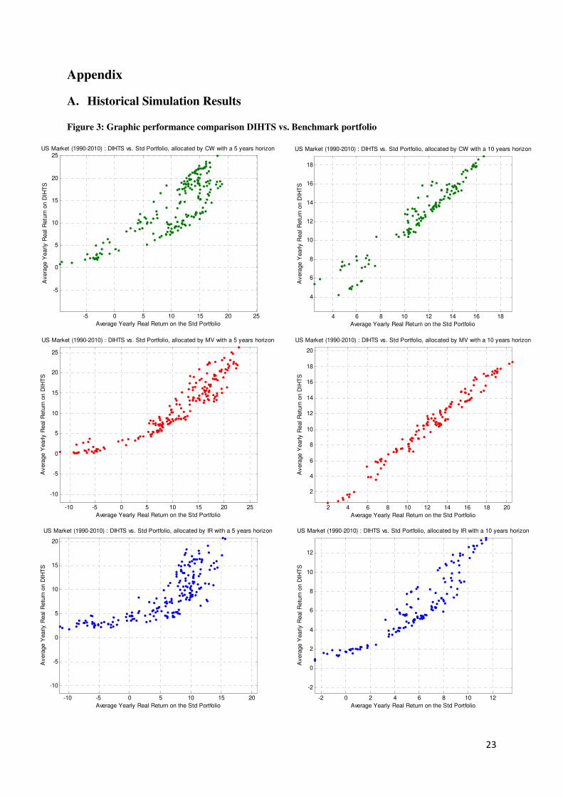
A. Historical Simulation Results
Figure 3: Graphic performance comparison DIHTS vs. Benchmark portfolio
-5 0 5 10 15 20 25
-5
0
5
10
15
20
25
Average Yearly Real Return on the Std Portfolio
Avera
ge Y
early R
eal R
etu
rn o
n D
IHT
S
US Market (1990-2010) : DIHTS vs. Std Portfolio, allocated by CW with a 5 years horizon
4 6 8 10 12 14 16 18
4
6
8
10
12
14
16
18
Average Yearly Real Return on the Std Portfolio
Avera
ge Y
early R
eal R
etu
rn o
n D
IHT
S
US Market (1990-2010) : DIHTS vs. Std Portfolio, allocated by CW with a 10 years horizon
-10 -5 0 5 10 15 20 25
-10
-5
0
5
10
15
20
25
Average Yearly Real Return on the Std Portfolio
Avera
ge Y
early R
eal R
etu
rn o
n D
IHT
S
US Market (1990-2010) : DIHTS vs. Std Portfolio, allocated by MV with a 5 years horizon
2 4 6 8 10 12 14 16 18 20
2
4
6
8
10
12
14
16
18
20
Average Yearly Real Return on the Std Portfolio
Avera
ge Y
early R
eal R
etu
rn o
n D
IHT
S
US Market (1990-2010) : DIHTS vs. Std Portfolio, allocated by MV with a 10 years horizon
-10 -5 0 5 10 15 20
-10
-5
0
5
10
15
20
Average Yearly Real Return on the Std Portfolio
Avera
ge Y
early R
eal R
etu
rn o
n D
IHT
S
US Market (1990-2010) : DIHTS vs. Std Portfolio, allocated by IR with a 5 years horizon
-2 0 2 4 6 8 10 12
-2
0
2
4
6
8
10
12
Average Yearly Real Return on the Std Portfolio
Avera
ge Y
early R
eal R
etu
rn o
n D
IHT
S
US Market (1990-2010) : DIHTS vs. Std Portfolio, allocated by IR with a 10 years horizon

24
Figure 4: Efficient frontier estimation
0 5 10 15 20 25 30 35 40 45-10
-5
0
5
10
15
20
25
30
Volatility of the NAV
Avera
ge Y
early R
eal R
etu
rn
US Market (1990-2010) : DIHTS vs. Benchmark Efficient Frontier
Allocated by CW with a 5 years horizon
EF DIHTS
DIHTS
EF Benchmark
Benchmark
0 20 40 60 80 1002
4
6
8
10
12
14
16
18
20
Volatility of the NAV
Avera
ge Y
early R
eal R
etu
rn
US Market (1990-2010) : DIHTS vs. Benchmark Efficient Frontier
Allocated by CW with a 10 years horizon
EF DIHTS
DIHTS
EF Benchmark
Benchmark
0 10 20 30 40 50-15
-10
-5
0
5
10
15
20
25
30
Volatility of the NAV
Avera
ge Y
early R
eal R
etu
rn
US Market (1990-2010) : DIHTS vs. Benchmark Efficient Frontier
Allocated by MV with a 5 years horizon
EF DIHTS
DIHTS
EF Benchmark
Benchmark
0 20 40 60 80 100 1200
5
10
15
20
25
Volatility of the NAV
Avera
ge Y
early R
eal R
etu
rnUS Market (1990-2010) : DIHTS vs. Benchmark Efficient Frontier
Allocated by MV with a 10 years horizon
EF DIHTS
DIHTS
EF Benchmark
Benchmark
0 5 10 15 20 25 30 35 40 45-15
-10
-5
0
5
10
15
20
25
Volatility of the NAV
Avera
ge Y
early R
eal R
etu
rn
US Market (1990-2010) : DIHTS vs. Benchmark Efficient Frontier
Allocated by IR with a 5 years horizon
EF DIHTS
DIHTS
EF Benchmark
Benchmark
0 5 10 15 20 25 30 35 40 45-4
-2
0
2
4
6
8
10
12
14
Volatility of the NAV
Avera
ge Y
early R
eal R
etu
rn
US Market (1990-2010) : DIHTS vs. Benchmark Efficient Frontier
Allocated by IR with a 10 years horizon
EF DIHTS
DIHTS
EF Benchmark
Benchmark
25
Figure 5 : Estimation of the mean Alpha values of the DIHTS and its 90% confidence interval
Months
Alp
ha
Mean Alpha value and 90% confidence interval
US Market (1990-2010) : DIHTS allocated by CW with a 5 years horizon
5 10 15 20 25 30 35 40 45 50 550
0.1
0.2
0.3
0.4
0.5
0.6
0.7
0.8
0.9
1
Months
Alp
ha
Mean Alpha value and 90% confidence interval
US Market (1990-2010) : DIHTS allocated by CW with a 10 years horizon
10 20 30 40 50 60 70 80 90 100 1100
0.1
0.2
0.3
0.4
0.5
0.6
0.7
0.8
0.9
1
Months
Alp
ha
Mean Alpha value and 90% confidence interval
US Market (1990-2010) : DIHTS allocated by MV with a 5 years horizon
5 10 15 20 25 30 35 40 45 50 550
0.1
0.2
0.3
0.4
0.5
0.6
0.7
0.8
0.9
1
Months
Alp
ha
Mean Alpha value and 90% confidence interval
US Market (1990-2010) : DIHTS allocated by MV with a 10 years horizon
10 20 30 40 50 60 70 80 90 100 1100
0.1
0.2
0.3
0.4
0.5
0.6
0.7
0.8
0.9
1
Months
Alp
ha
Mean Alpha value and 90% confidence interval
US Market (1990-2010) : DIHTS allocated by IR with a 5 years horizon
5 10 15 20 25 30 35 40 45 50 550
0.1
0.2
0.3
0.4
0.5
0.6
0.7
0.8
0.9
1
Months
Alp
ha
Mean Alpha value and 90% confidence interval
US Market (1990-2010) : DIHTS allocated by IR with a 10 years horizon
10 20 30 40 50 60 70 80 90 100 1100
0.1
0.2
0.3
0.4
0.5
0.6
0.7
0.8
0.9
1

26
Figure 6: Mean Allocation
Months
Allo
cation
Mean Allocation
US Market (1990-2010) : DIHTS allocated by CW with a 5 years horizon
0 10 20 30 40 50 600
0.05
0.1
0.15
0.2
0.25
0.3
0.35
0.4
0.45
0.5
ZCN
SPX
REIT
GSCI
Months
Allo
cation
Mean Allocation
US Market (1990-2010) : DIHTS allocated by CW with a 10 years horizon
0 20 40 60 80 100 1200
0.05
0.1
0.15
0.2
0.25
0.3
0.35
0.4
0.45
0.5
ZCN
SPX
REIT
GSCI
Months
Allo
cation
Mean Allocation
US Market (1990-2010) : DIHTS allocated by MV with a 5 years horizon
0 10 20 30 40 50 600
0.05
0.1
0.15
0.2
0.25
0.3
0.35
0.4
0.45
0.5ZCN
SPX
REIT
GSCI
Months
Allo
cation
Mean Allocation
US Market (1990-2010) : DIHTS allocated by MV with a 10 years horizon
0 20 40 60 80 100 1200
0.05
0.1
0.15
0.2
0.25
0.3
0.35
0.4
0.45
0.5
ZCN
SPX
REIT
GSCI
Months
Allo
cation
Mean Allocation
US Market (1990-2010) : DIHTS allocated by IR with a 5 years horizon
0 10 20 30 40 50 600
0.05
0.1
0.15
0.2
0.25
0.3
0.35
0.4
0.45
0.5
ZCN
SPX
REIT
GSCI
Months
Allo
cation
Mean Allocation
US Market (1990-2010) : DIHTS allocated by IR with a 10 years horizon
0 20 40 60 80 100 1200
0.05
0.1
0.15
0.2
0.25
0.3
0.35
0.4
0.45
0.5
ZCN
SPX
REIT
GSCI

27
Table 1: Horizon sensitivity of the DIHTS vs. the Benchmark Portfolio
CW
MV
IR
DIHTS PTF DIHTS PTF DIHTS PTF
60,27% 33,80% 5,46% 3,65%
(28,6%) (21,93%) (1,8%) (0,63%)
44,03% 28,96% 6,89% 4,79%
(18,0%) (11,57%) (1,8%) (0,87%)
34,23% 24,52% 8,65% 6,09%
(12,4%) (7,61%) (1,8%) (1,02%)
26,89% 20,27% 10,45% 7,47%
(8,2%) (6,50%) (1,8%) (0,97%)
21,56% 17,13% 12,24% 9,00%
(5,8%) (5,05%) (1,8%) (0,96%)
17,92% 14,80% 14,22% 10,83%
(4,2%) (3,63%) (2,2%) (1,32%)
Fail Rate IR ToR
0,00%
0,00% 0,00%
1,91%
1,18%
1,66%
12,44%
Horizon (Years)
5
6
7
8
9
10
0,00%
0,00%
0,00%
0,00%
0,00%
DIHTS PTF DIHTS PTF DIHTS PTF
53,80% 29,69% 6,09% 6,59%
(27,1%) (26,33%) (2,2%) (1,29%)
42,26% 26,17% 7,66% 8,53%
(21,5%) (15,03%) (2,5%) (1,64%)
34,10% 22,11% 9,62% 10,74%
(14,0%) (8,11%) (2,7%) (2,09%)
27,85% 18,47% 11,70% 13,11%
(10,5%) (6,20%) (2,6%) (2,35%)
22,37% 15,82% 13,70% 15,75%
(8,6%) (5,05%) (2,5%) (2,78%)
18,56% 13,72% 15,90% 18,99%
(6,5%) (3,86%) (2,9%) (3,86%)
Horizon (Years)
Fail Rate IR ToR
5 0,00% 13,47%
6 0,00% 8,84%
7 0,00% 0,00%
10 0,00% 0,00%
8 0,00% 1,27%
9 0,00% 0,00%
DIHTS PTF DIHTS PTF DIHTS PTF
59,48% 24,35% 7,17% 7,36%
(30,2%) (32,65%) (3,2%) (1,39%)
48,70% 22,55% 8,91% 9,30%
(26,2%) (20,50%) (3,5%) (1,75%)
38,41% 20,82% 10,29% 11,45%
(18,3%) (11,31%) (3,9%) (2,03%)
32,06% 18,42% 11,18% 13,57%
(13,6%) (10,61%) (3,9%) (2,03%)
29,30% 15,91% 12,08% 15,87%
(13,6%) (9,53%) (3,7%) (2,10%)
25,56% 13,89% 13,33% 18,55%
(12,4%) (7,95%) (3,5%) (2,36%)10 0,00% 7,52%
8 0,00% 8,28%
9 0,00% 9,66%
6 0,00% 21,55%
7 0,00% 9,47%
Horizon (Years)
Fail Rate IR ToR
5 0,00% 20,73%

28
Table 2: Allocation horizon sensitivity analysis
CW
MV
IR
Horizon
(Years)ZCN SPX REIT GSCI
23,5% 24,9% 24,9% 24,9%
(22,2%) (14,3%) (10,2%) (7,9%)
19,0% 26,6% 26,6% 26,6%
(19,7%) (12,2%) (8,3%) (6,2%)
13,9% 28,3% 28,3% 28,3%
(16,4%) (9,2%) (5,5%) (3,4%)
9,9% 29,7% 29,7% 29,7%
(12,9%) (6,2%) (2,6%) (0,7%)
7,6% 30,5% 30,5% 30,5%
(9,8%) (3,6%) (0,3%) (1,5%)
5,7% 31,2% 31,2% 31,2%
(6,9%) (1,4%) (1,6%) (3,3%)
5
6
7
8
9
10
Horizon
(Years)ZCN SPX REIT GSCI
28,1% 29,9% 5,3% 35,0%
(22,2%) (17,3%) (14,9%) (13,9%)
24,1% 31,7% 5,7% 37,2%
(19,7%) (15,9%) (13,9%) (13,3%)
19,3% 33,7% 6,1% 39,7%
(16,4%) (14,2%) (13,1%) (12,9%)
14,9% 35,5% 6,6% 41,9%
(12,9%) (13,1%) (12,8%) (13,1%)
12,3% 36,5% 6,9% 43,3%
(9,8%) (12,7%) (13,0%) (13,6%)
9,8% 37,6% 7,2% 44,6%
(6,9%) (12,8%) (13,6%) (14,3%)
5
6
7
8
9
10
Horizon
(Years)ZCN SPX REIT GSCI
31,6% 32,2% 19,8% 14,7%
(22,2%) (16,5%) (12,9%) (10,9%)
29,0% 33,6% 20,3% 15,7%
(19,7%) (14,4%) (10,9%) (9,2%)
25,9% 35,2% 20,6% 17,2%
(16,4%) (11,5%) (8,3%) (7,3%)
22,7% 36,8% 21,2% 18,3%
(12,9%) (8,7%) (6,9%) (6,8%)
20,3% 38,0% 22,4% 18,3%
(9,8%) (6,9%) (7,1%) (7,8%)
17,8% 39,3% 23,8% 18,3%
(6,9%) (7,1%) (8,3%) (9,4%)
5
6
7
8
9
10

29
Table 3: Parameter sensitivity analysis for the DIHTS
CW
MV
Mu
Eta
FR 0,0% 0,0% 0,0% 5,3% 6,0%
ToR 9,1% (1,8%) 13,1% (2,8%) 14,3% (2,1%) 12,2% (1,8%) 11,5% (1,5%)
IR 22,9% (4,0%) 20,4% (4,1%) 17,9% (4,1%) 17,2% (6,2%) 17,4% (6,1%)
FR 0,0% (0,0%) 0,0% (0,0%) 0,0% (0,0%) 5,3% (0,0%) 6,0% (0,0%)
ToR 9,0% (1,8%) 13,1% (2,8%) 14,3% (2,1%) 12,2% (1,8%) 11,5% (1,5%)
IR 22,9% (4,1%) 20,4% (4,1%) 17,9% (4,2%) 17,2% (6,2%) 17,4% (6,1%)
FR 0,0% (0,0%) 0,0% (0,0%) 0,0% (0,0%) 5,3% (0,0%) 6,0% (0,0%)
ToR 8,8% (1,8%) 12,9% (2,8%) 14,2% (2,2%) 12,2% (1,8%) 11,5% (1,5%)
IR 22,8% (4,1%) 20,5% (4,1%) 17,9% (4,2%) 17,2% (6,2%) 17,4% (6,1%)
FR 0,0% (0,0%) 0,0% (0,0%) 0,0% (0,0%) 5,3% (0,0%) 6,0% (0,0%)
ToR 8,8% (1,8%) 12,8% (2,8%) 14,2% (2,2%) 12,2% (1,8%) 11,5% (1,5%)
IR 22,8% (4,1%) 20,5% (4,1%) 17,9% (4,2%) 17,2% (6,2%) 17,4% (6,1%)
FR 0,0% (0,0%) 0,0% (0,0%) 0,0% (0,0%) 5,3% (0,0%) 6,0% (0,0%)
ToR 8,7% (1,8%) 12,7% (2,8%) 14,1% (2,2%) 12,2% (1,8%) 11,5% (1,5%)
IR 22,8% (4,1%) 20,5% (4,1%) 17,9% (4,2%) 17,2% (6,2%) 17,4% (6,1%)
FR 0,0% (0,0%) 0,0% (0,0%) 0,0% (0,0%) 5,3% (0,0%) 6,0% (0,0%)
ToR 8,7% (1,8%) 12,5% (2,7%) 14,1% (2,2%) 12,1% (1,8%) 11,5% (1,5%)
IR 22,8% (4,1%) 20,5% (4,1%) 0,179 (4,2%) 0,172 (6,2%) 0,174 (6,1%)
0.5%
1%
1.5%
2%
2.5%
10% 30% 50% 70% 90%
0%
Mu
Eta
FR 0,0% 0,0% 0,0% 9,0% 11,3%
ToR 10,0% (2,3%) 14,3% (3,8%) 16,0% (2,8%) 13,7% (2,9%) 12,8% (3,5%)
IR 23,4% (5,1%) 21,2% (5,6%) 18,6% (6,5%) 17,4% (7,7%) 16,8% (7,7%)
FR 0,0% (0,0%) 0,0% (0,0%) 0,0% (0,0%) 9,0% (0,0%) 11,3% (0,0%)
ToR 9,9% (2,3%) 14,2% (3,8%) 15,9% (2,8%) 13,7% (2,9%) 12,8% (3,5%)
IR 23,4% (5,1%) 21,2% (5,6%) 18,6% (6,5%) 17,5% (7,7%) 16,8% (7,7%)
FR 0,0% (0,0%) 0,0% (0,0%) 0,0% (0,0%) 9,0% (0,0%) 11,3% (0,0%)
ToR 9,8% (2,3%) 14,0% (3,8%) 15,9% (2,9%) 13,7% (3,0%) 12,8% (3,5%)
IR 23,4% (5,1%) 21,2% (5,7%) 18,6% (6,5%) 17,4% (7,7%) 16,8% (7,7%)
FR 0,0% (0,0%) 0,0% (0,0%) 0,0% (0,0%) 9,0% (0,0%) 11,3% (0,0%)
ToR 9,7% (2,2%) 13,9% (3,8%) 15,8% (2,9%) 13,7% (3,0%) 12,8% (3,5%)
IR 23,4% (5,1%) 21,2% (5,7%) 18,6% (6,5%) 17,4% (7,7%) 16,8% (7,7%)
FR 0,0% (0,0%) 0,0% (0,0%) 0,0% (0,0%) 9,0% (0,0%) 11,3% (0,0%)
ToR 9,6% (2,3%) 13,7% (3,8%) 15,8% (3,0%) 13,7% (3,0%) 12,8% (3,5%)
IR 23,4% (5,2%) 21,2% (5,7%) 18,6% (6,5%) 17,5% (7,8%) 16,8% (7,7%)
FR 0,0% (0,0%) 0,0% (0,0%) 0,0% (0,0%) 9,0% (0,0%) 11,3% (0,0%)
ToR 9,5% (2,3%) 13,6% (3,8%) 15,7% (3,0%) 13,7% (3,0%) 12,8% (3,5%)
IR 23,4% (5,1%) 21,2% (5,7%) 0,186 (6,5%) 0,175 (7,8%) 0,168 (7,7%)
0.5%
1%
1.5%
2%
2.5%
10% 30% 50% 70% 90%
0%

30
IR
Mu
Eta
FR 0,0% 0,0% 0,0% 25,6% 20,3%
ToR 9,6% (2,3%) 12,1% (2,4%) 13,5% (3,6%) 11,3% (2,8%) 11,1% (2,0%)
IR 26,7% (7,8%) 29,1% (11,0%) 25,6% (12,4%) 19,8% (13,5%) 20,6% (12,0%)
FR 0,0% (0,0%) 0,0% (0,0%) 0,0% (0,0%) 25,6% (0,0%) 20,3% (0,0%)
ToR 9,5% (2,3%) 12,0% (2,4%) 13,5% (3,5%) 11,3% (2,8%) 11,1% (2,0%)
IR 26,7% (7,8%) 29,1% (11,0%) 25,6% (12,4%) 19,7% (13,4%) 20,6% (12,0%)
FR 0,0% (0,0%) 0,0% (0,0%) 0,0% (0,0%) 25,6% (0,0%) 20,3% (0,0%)
ToR 9,4% (2,4%) 11,7% (2,2%) 13,3% (3,5%) 11,3% (2,8%) 11,1% (2,0%)
IR 26,7% (7,8%) 29,2% (11,1%) 25,6% (12,4%) 19,7% (13,4%) 20,6% (12,0%)
FR 0,0% (0,0%) 0,0% (0,0%) 0,0% (0,0%) 25,6% (0,0%) 19,5% (0,0%)
ToR 9,3% (2,3%) 11,5% (2,0%) 13,2% (3,5%) 11,3% (2,8%) 11,1% (1,9%)
IR 26,6% (7,8%) 29,2% (11,1%) 25,5% (12,4%) 19,7% (13,4%) 20,7% (11,8%)
FR 0,0% (0,0%) 0,0% (0,0%) 0,0% (0,0%) 25,6% (0,0%) 19,5% (0,0%)
ToR 9,2% (2,3%) 11,3% (1,9%) 13,1% (3,6%) 11,2% (2,7%) 11,1% (1,9%)
IR 26,6% (7,7%) 29,3% (11,2%) 25,5% (12,4%) 19,8% (13,4%) 20,7% (11,8%)
FR 0,0% (0,0%) 0,0% (0,0%) 0,0% (0,0%) 25,6% (0,0%) 19,5% (0,0%)
ToR 9,1% (2,2%) 11,1% (1,9%) 12,9% (3,3%) 11,2% (2,7%) 11,1% (1,9%)
IR 26,6% (7,7%) 29,3% (11,2%) 0,255 (12,4%) 0,198 (13,5%) 0,207 (11,8%)
0.5%
1%
1.5%
2%
2.5%
10% 30% 50% 70% 90%
0%

31
B. Bootstrapped Simulation Results Figure 7: Graphic performance comparison DIHTS vs. Benchmark portfolio

32
Figure 8: Efficient frontier estimation
33
Figure 9: Estimation of the mean Alpha values of the DIHTS and its 90% confidence interval
Months
Alp
ha
Mean Alpha value and 90% confidence interval
US Market Bootstrapped Simulation : DIHTS allocated by CW with a 5 years horizon
5 10 15 20 25 30 35 40 45 50 550
0.1
0.2
0.3
0.4
0.5
0.6
0.7
0.8
0.9
1
Months
Alp
ha
Mean Alpha value and 90% confidence interval
US Market Bootstrapped Simulation : DIHTS allocated by CW with a 10 years horizon
10 20 30 40 50 60 70 80 90 100 1100
0.1
0.2
0.3
0.4
0.5
0.6
0.7
0.8
0.9
1
Months
Alp
ha
Mean Alpha value and 90% confidence interval
US Market Bootstrapped Simulation : DIHTS allocated by MV with a 5 years horizon
5 10 15 20 25 30 35 40 45 50 550
0.1
0.2
0.3
0.4
0.5
0.6
0.7
0.8
0.9
1
Months
Alp
ha
Mean Alpha value and 90% confidence interval
US Market Bootstrapped Simulation : DIHTS allocated by MV with a 10 years horizon
10 20 30 40 50 60 70 80 90 100 1100
0.1
0.2
0.3
0.4
0.5
0.6
0.7
0.8
0.9
1
Months
Alp
ha
Mean Alpha value and 90% confidence interval
US Market Bootstrapped Simulation : DIHTS allocated by IR with a 5 years horizon
5 10 15 20 25 30 35 40 45 50 550
0.1
0.2
0.3
0.4
0.5
0.6
0.7
0.8
0.9
1
Months
Alp
ha
Mean Alpha value and 90% confidence interval
US Market Bootstrapped Simulation : DIHTS allocated by IR with a 10 years horizon
10 20 30 40 50 60 70 80 90 100 1100
0.1
0.2
0.3
0.4
0.5
0.6
0.7
0.8
0.9
1

34
Figure 10: Mean allocation
Table 4: Horizon sensitivity of the DIHTS vs. the Benchmark Portfolio
CW
Months
Allo
cation
Mean Allocation
US Market Bootstrapped Simulation : DIHTS allocated by CW with a 5 years horizon
0 10 20 30 40 50 600
0.05
0.1
0.15
0.2
0.25
0.3
0.35
0.4
0.45
0.5
ZCN
SPX
REIT
GSCI
Months
Allo
cation
Mean Allocation
US Market Bootstrapped Simulation : DIHTS allocated by CW with a 10 years horizon
0 20 40 60 80 100 1200
0.05
0.1
0.15
0.2
0.25
0.3
0.35
0.4
0.45
0.5
ZCN
SPX
REIT
GSCI
Months
Allo
cation
Mean Allocation
US Market Bootstrapped Simulation : DIHTS allocated by MV with a 5 years horizon
0 10 20 30 40 50 600
0.05
0.1
0.15
0.2
0.25
0.3
0.35
0.4
0.45
0.5
ZCN
SPX
REIT
GSCI
Months
Allo
cation
Mean Allocation
US Market Bootstrapped Simulation : DIHTS allocated by MV with a 10 years horizon
0 20 40 60 80 100 1200
0.05
0.1
0.15
0.2
0.25
0.3
0.35
0.4
0.45
0.5
ZCN
SPX
REIT
GSCI
Months
Allo
cation
Mean Allocation
US Market Bootstrapped Simulation : DIHTS allocated by IR with a 5 years horizon
0 10 20 30 40 50 600
0.05
0.1
0.15
0.2
0.25
0.3
0.35
0.4
0.45
0.5
ZCN
SPX
REIT
GSCI
Months
Allo
cation
Mean Allocation
US Market Bootstrapped Simulation : DIHTS allocated by IR with a 10 years horizon
0 20 40 60 80 100 1200
0.05
0.1
0.15
0.2
0.25
0.3
0.35
0.4
0.45
0.5
ZCN
SPX
REIT
GSCI
35
MV
IR
Table 5: Allocation horizon sensitivity analysis for the DIHTS allocated by CW.
CW
Horizon (Years)
Fail Rate IR ToR PLGF
DIHTS PTF DIHTS PTF DIHTS PTF
5 7,92% 12,58% 59,01% 70,32% 6,57% 3,80% ‐5,47% (30,2%) (33,59%) (3,5%) (0,91%) (13,27%)
6 8,33% 11,10% 46,28% 46,80% 7,40% 4,95% ‐2,90% (22,6%) (22,92%) (3,4%) (1,23%) (11,42%)
7 7,78% 9,39% 39,24% 38,24% 8,76% 6,31% ‐1,49% (10,6%) (10,16%) (3,7%) (1,73%) (10,13%)
8 7,42% 4,99% 20,53% 20,57% 9,90% 7,91% 0,85% (3,2%) (3,09%) (4,0%) (2,28%) (9,56%)
9 10,31% 7,43% 12,85% 12,91% 11,09% 9,45% ‐1,18% (1,0%) (0,81%) (4,7%) (3,11%) (11,20%)
10 10,42% 6,29% 8,94% 9,44% 12,51% 11,26% 0,52% (0,7%) (0,66%) (5,4%) (3,75%) (10,42%)
Horizon (Years)
Fail Rate IR ToR PLGF
DIHTS PTF DIHTS PTF DIHTS PTF
5 10,10% 16,58% 122,92% 107,33% 7,60% 5,71% ‐6,54% (80,4%) (73,70%) (4,2%) (1,82%) (13,00%)
6 10,23% 14,58% 30,46% 32,15% 8,53% 7,14% ‐4,75% (8,6%) (9,03%) (4,2%) (2,59%) (11,31%)
7 9,81% 13,55% 31,91% 31,01% 10,05% 8,69% ‐3,87% (13,2%) (12,77%) (4,7%) (3,36%) (8,96%)
8 10,44% 9,03% 24,90% 24,30% 11,86% 11,01% ‐0,30% (1,8%) (2,90%) (5,8%) (4,39%) (9,52%)
9 13,63% 10,76% ‐22,30% ‐19,70% 12,85% 12,97% ‐1,47% (31,5%) (27,87%) (6,5%) (5,69%) (11,59%)
10 13,45% 10,25% 15,60% 11,31% 14,04% 14,39% ‐0,26% (5,2%) (4,49%) (7,3%) (5,97%) (9,95%)
Horizon (Years)
Fail Rate IR ToR PLGF
DIHTS PTF DIHTS PTF DIHTS PTF
5 9,93% 16,17% 56,05% 51,79% 8,10% 6,17% ‐7,03% (21,4%) (19,95%) (4,9%) (2,38%) (13,31%)
6 10,55% 14,19% 45,52% 47,95% 9,13% 7,79% ‐5,82% (18,8%) (21,36%) (4,9%) (3,02%) (12,81%)
7 8,83% 12,24% 25,64% 31,05% 10,66% 9,37% ‐5,92% (15,2%) (21,26%) (5,3%) (3,77%) (14,60%)
8 9,63% 8,70% 29,69% 32,00% 11,68% 11,27% ‐1,01% (9,0%) (9,78%) (6,1%) (4,69%) (12,55%)
9 13,33% 10,55% 22,52% 21,03% 13,26% 13,63% ‐4,56% (6,2%) (4,92%) (6,6%) (5,61%) (12,93%)
10 12,14% 8,60% 4,94% 4,89% 15,44% 16,14% ‐2,09% (7,0%) (6,91%) (8,2%) (7,61%) (13,75%)

36
MV
IR
Horizon \
Allocation ZCN SPX REIT GSCI
5 16,8% 26,9% 26,9% 26,9%
(10,9%) (1,8%) (1,4%) (2,7%)
6 16,2% 27,1% 27,1% 27,1%
(10,3%) (2,4%) (0,6%) (1,9%)
7 15,0% 27,7% 27,7% 27,7%
(8,6%) (1,7%) (1,1%) (2,4%)
8 14,5% 27,7% 27,7% 27,7%
(7,3%) (1,8%) (0,7%) (1,9%)
9 14,3% 27,5% 27,5% 27,5%
(5,9%) (1,2%) (1,0%) (2,1%)
10 14,5% 27,4% 27,4% 27,4%
(5,1%) (1,0%) (0,7%) (1,6%)
Horizon \
Allocation ZCN SPX REIT GSCI
5 17,9% 35,6% 16,9% 26,9%
(10,8%) (6,9%) (7,3%) (7,8%)
6 17,6% 36,1% 16,5% 27,0%
(10,1%) (7,3%) (7,4%) (7,8%)
7 16,6% 36,9% 16,7% 27,5%
(8,7%) (7,3%) (7,5%) (7,9%)
8 16,1% 35,2% 16,8% 29,4%
(7,4%) (6,6%) (6,8%) (7,2%)
9 16,3% 35,8% 16,3% 28,4%
(5,6%) (6,7%) (7,1%) (7,4%)
10 16,9% 35,8% 15,8% 27,8%
(5,1%) (7,2%) (7,4%) (7,7%)
Horizon \
Allocation ZCN SPX REIT GSCI
5 17,3% 22,5% 35,5% 21,6%
(10,7%) (5,7%) (6,1%) (6,6%)
6 17,1% 22,9% 35,7% 21,4%
(10,2%) (5,9%) (5,9%) (6,4%)
7 15,9% 21,9% 37,0% 22,7%
(8,7%) (6,3%) (6,5%) (6,9%)
8 15,8% 25,3% 35,9% 20,1%
(7,5%) (5,7%) (5,8%) (6,1%)
9 14,9% 24,8% 35,9% 20,4%
(5,8%) (5,5%) (5,7%) (6,1%)
10 14,5% 23,2% 36,3% 21,3%
(5,0%) (5,5%) (5,7%) (5,9%)

37
References
Amenc, Noël., Lionel. Martellini, and Volker. Ziemann. "Inflation‐Hedging Properties of Real Assets and Implications for Asset–Liability Management." Journal of Portfolio Management, 2009: Summer 2009, Vol. 35, No. 4: pp. 94‐110.
Ang, A., G Bekaert, and M Wei. "The term structure of real rates and expected inflation." Journal of Finance, 2008: 63, p797‐849.
Attié, Alexander P, and Shaun K Roache. "Inflation Hedging for Long‐Term Investors." IMF Working Paper, April 2009.
Barclays Capital Research. "Dividend Swap Indices, Access to equity income streams made easy." Analysts Index Products Research. April 2008.
Black, Fischer, and Robert Jones. "Simplifying portfolio insurance." Journal of Portfolio Management 14, no. 1 (Fall 1987): p48‐51.
Bodie, Zvi. "Common Stocks as a Hedge Against Inflation." The Journal of Finance, May 1976: VOL. XXXI, NO. 2.
Bodie, Zvi. "Inflation, index‐linked bonds, and asset allocation." Journal of Portfolio Management Vol. 16, no. Issue 2 (Winter 1990): p48‐53.
Bodie, Zvie. "Commodity futures as a hedge against inflation." The Journal of Portfolio Management, Spring 1983: Vol. 9, No. 3: pp. 12‐17.
Brennan, Michael J., and Yihong Xia. "Dynamic Asset Allocation under Inflation." The Journal of Finance, 2002: 1201–1238.
Brière, Marie & Signori, Ombretta. "Inflation‐hedging portfolios in Different Regimes." Working Papers, Universite Libre de Bruxelles, 2009: CEB 09‐047.RS, ULB.
Brière, Marie, and Ombretta Signori. "Inflation‐hedging portfolios in Different Regimes." Working Paper. 2010.
D'Amico, S, D Kim, and M Wei. "Tips from TIPS: The informational content of Treasury Inflation‐Protected Security prices." Federal Reserve Board, Working Paper, 2009.
Fisher, Irvine. The Rate of Interest. New York: Macmillan, 1907.
Leland, Hayne E. "Who Should Buy Portfolio Insurance?" The Journal of Finance 35, no. 2 (Mai 1980).
Leland, Hayne E., and Mark Rubinstein. "Replicating Options with Positions in Stocks and Cash." Financial Analysts Journal, 1981: 63‐72.
Newell, Graeme, and Chris Eves Lincoln. "The Role of U.S. Farmland in Real Estate Portfolios." Journal of Real Estate Portfolio Management, 2009: 317‐328.
Park, Jeong Yun, Donald J. Mullineaux, and It‐Keong Chew. "Are REITs Inflation Hedges?" The Journal of Real Estate Finance and Economics, 1990: 91‐103.

38
Perold, Andre F., and William F. Sharpe. " Dynamic Strategies for Asset Allocation." Financial Analyst Journal, 1988: 16‐27.
Politis, Dimitris N., and Halbert White. "Automatic Block‐Length Selection for the Dependent Bootstrap." Econometric Reviews Vol. 23, no. Issue 1 (Feb 2004): p53‐70.
Rubens, Jack H, Michael T Bond, and James R Webb. "The Inflation‐Hedging Effectiveness of Real Estate." Journal of Real Estate Research, 2009: 45‐55.
Van den Goorbergh, Rob., Onno. W. Steenbeek, R. Molenaar, and Peter Vlaar. "Risk Models after the Credit Crisis." SSRN Working Paper Series, December 2009.
Washburn, Courtland L., and Clark S. Binkley. "Do Forest Assets Hedge Inflation?" Land Economics, 1993: 215‐224 .
Zvie, Bodie. "Commodity futures as a hedge against inflation." The Journal of Portfolio Management, Spring 1983: Vol. 9, No. 3: pp. 12‐17.

39
List of Figures
Figure 1: Example of a joint simulation of nominal rates and inflation using block bootstrapping ..... 18 Figure 2 : DIHTS – Benchmark Fail Rate Enhancement Horizon Sensitivity .......................................... 20 Figure 3: Graphic performance comparison DIHTS vs. Benchmark portfolio ....................................... 23 Figure 4: Efficient frontier estimation ................................................................................................... 24 Figure 5 : Estimation of the mean Alpha values of the DIHTS and its 90% confidence interval ........... 25 Figure 6: Mean Allocation ..................................................................................................................... 26 Table 1: Horizon sensitivity of the DIHTS vs. the Benchmark Portfolio ................................................ 27 Table 2: Allocation horizon sensitivity analysis ..................................................................................... 28 Table 3: Parameter sensitivity analysis for the DIHTS ........................................................................... 29 Figure 7: Graphic performance comparison DIHTS vs. Benchmark portfolio ....................................... 31 Figure 8: Efficient frontier estimation ................................................................................................... 32 Figure 9: Estimation of the mean Alpha values of the DIHTS and its 90% confidence interval ............ 33 Figure 10: Mean allocation .................................................................................................................... 34 Table 4: Horizon sensitivity of the DIHTS vs. the Benchmark Portfolio ................................................ 34 Table 5: Allocation horizon sensitivity analysis for the DIHTS allocated by CW. .................................. 35
List of Tables
Table 1: Horizon sensitivity of the DIHTS vs. the Benchmark Portfolio ................................................ 27 Table 2: Allocation horizon sensitivity analysis ..................................................................................... 28 Table 3: Parameter sensitivity analysis for the DIHTS ........................................................................... 29 Table 4: Horizon sensitivity of the DIHTS vs. the Benchmark Portfolio ................................................ 34 Table 5: Allocation horizon sensitivity analysis for the DIHTS allocated by CW. .................................. 35
Top Related