


Languages
Pages
Legal


A Computational Approach to SolventSelection for Biphasic Reaction Systems
Von der Fakultat fur Mathematik, Informatik und Naturwissenschaften der
RWTH Aachen University zur Erlangung des akademischen Grades einer
Doktorin der Ingenieurwissenschaften genehmigte Dissertation
vorgelegt von
Diplom-Chemikerin
Martina Peters
aus Bitburg
Berichter: Universitatsprofessor Dr. rer. nat. Walter Leitner
Universitatsprofessor Dr.-Ing. Andreas Pfennig
Tag der mundlichen Prufung: 15.12.2008
Diese Dissertation ist auf den Internetseiten der Hochschulbibliothek online verfugbar.


The present doctoral thesis was carried out at the Institute of Technical and Macro-
molecular Chemistry at RWTH Aachen University, Germany, under the supervision of
Prof. Dr. Walter Leitner from 12/2005 until 12/2008. It was part of and financially sup-
ported by the DFG graduate school 1166 BioNoCo - Biocatalysis using non-conventional
media.
Parts of this thesis have already been published:
• M. Peters, M. Zavrel, J. Kahlen, T. Schmidt, M. Ansorge-Schumacher, W. Leitner,
J. Buchs, L. Greiner, A. C. Spiess, Eng. Life Sci. 2008, 8, 546-552.
• M. Peters, L. Greiner, K. Leonhard, AICHE J. 2008, 54, 2729-2734.
• A. C. Spiess, W. Eberhard, M. Peters, M. F. Eckstein, L. Greiner, J. Buchs, Chem.
Eng. Proc. 2008, 47, 1034-1041.
• M. Peters, M. F. Eckstein, G. Hartjen, A. C. Spiess, W. Leitner, L. Greiner, Ind.
Eng. Chem. Res. 2007, 46, 7073-7078.
• M. F. Eckstein, J. Lembrecht, J. Schumacher, W. Eberhard, A. C. Spiess, M. Pe-
ters, C. Roosen, L. Greiner, W. Leitner, U. Kragl, Adv. Synth. Catal. 2006, 348,
1597-1604.
• M. F. Eckstein, M. Peters, J. Lembrecht, A. C. Spiess, L. Greiner, Adv. Synth.
Catal. 2006, 348, 1591-1596.

Abstract
Biphasic reaction systems with a reactive and a non-reactive phase are widespread in
technical applications. The non-reactive phase serves as a reservoir of dissolved substrates
at high concentrations and allows for the extraction of the product during the reaction.
The proper choice of the phase combination will have manifold influence on catalytic
parameters such as activity, selectivity, and stability, but also on maximum conversion or
yield. To optimize such biphasic reactions, conversion and yield constitute concise targets
of practical relevance for a rational solvent screening which requires thermodynamic
information on coupled reactions and phase equilibria as input. Usually, the experimental
determination of these data requires considerable laboratory effort.
To minimize the experimental effort and to enlarge the dataspace for optimization, an
in silico solvent screening for maximum conversion and yield in different biphasic cat-
alyzed reactions is evaluated. The primary target of the investigations is in biocatalytic
applications as these benefit greatly from the addition of organic non-reactive media to
the reactive aqueous phase. The conductor-like screening model for realistic solvation
(COSMO-RS) is used for the prediction of solute partitioning between organic solvents
and a reaction medium. Although the calculated results show significant absolute de-
viations, COSMO-RS still predicts the correct trends for the partition coefficients of
solutes in different solvents. Furthermore, a combination of statistical thermodynam-
ics and classical quantum mechanics is used for the prediction of the reaction equilibria.
The calculated overall reaction equilibrium using the calculated partition coefficients and
the calculated equilibrium constants again results in the prediction of the best solvent
combination regarding conversion and yield. Extending the approach with numerical
simulations provides a more detailed insight into the reaction system.

Contents
Nomenclature v
List of figures ix
List of tables xi
List of schemes xiii
1. Introduction 1
1.1. Industrial applications of solvents . . . . . . . . . . . . . . . . . . . . . . 2
1.2. Molecular models for fluid phases . . . . . . . . . . . . . . . . . . . . . . 3
1.2.1. Constraints for fluid-phase models . . . . . . . . . . . . . . . . . . 3
1.2.2. Inter- and intramolecular potential energy . . . . . . . . . . . . . 5
1.2.3. Fundamental equations . . . . . . . . . . . . . . . . . . . . . . . . 5
1.2.4. Implicit models for condensed phases . . . . . . . . . . . . . . . . 6
1.2.4.1. Continuum solvation models . . . . . . . . . . . . . . . . 7
1.2.4.2. Quantum mechanics . . . . . . . . . . . . . . . . . . . . 7
1.2.4.3. COSMO . . . . . . . . . . . . . . . . . . . . . . . . . . . 9
1.2.5. Excess function models . . . . . . . . . . . . . . . . . . . . . . . . 11
1.2.5.1. Basics of excess function models . . . . . . . . . . . . . . 11
1.2.5.2. Group interaction models - UNIFAC . . . . . . . . . . . 12
1.2.5.3. Surface charge interaction models - COSMO-RS . . . . . 15
1.3. Applications of fluid-phase models . . . . . . . . . . . . . . . . . . . . . . 20
1.4. Objective . . . . . . . . . . . . . . . . . . . . . . . . . . . . . . . . . . . 21
i
Contents
2. Mathematical analysis of biphasic reaction systems 25
2.1. Introduction . . . . . . . . . . . . . . . . . . . . . . . . . . . . . . . . . . 25
2.2. Materials and methods . . . . . . . . . . . . . . . . . . . . . . . . . . . . 25
2.2.1. Computational . . . . . . . . . . . . . . . . . . . . . . . . . . . . 25
2.2.2. Experimental . . . . . . . . . . . . . . . . . . . . . . . . . . . . . 26
2.3. Results and discussion . . . . . . . . . . . . . . . . . . . . . . . . . . . . 26
2.3.1. Mathematical description . . . . . . . . . . . . . . . . . . . . . . 27
2.3.2. Equilibrium constant . . . . . . . . . . . . . . . . . . . . . . . . . 30
2.3.3. Partition coefficients . . . . . . . . . . . . . . . . . . . . . . . . . 31
2.3.4. Co-substrate excess . . . . . . . . . . . . . . . . . . . . . . . . . . 32
2.3.5. Phase volume ratio . . . . . . . . . . . . . . . . . . . . . . . . . . 32
2.3.6. Experimental validation . . . . . . . . . . . . . . . . . . . . . . . 34
2.4. Conclusion . . . . . . . . . . . . . . . . . . . . . . . . . . . . . . . . . . . 39
3. Calculating partition coefficients using COSMO-RS 41
3.1. Introduction . . . . . . . . . . . . . . . . . . . . . . . . . . . . . . . . . . 41
3.2. Materials and methods . . . . . . . . . . . . . . . . . . . . . . . . . . . . 41
3.2.1. Computational . . . . . . . . . . . . . . . . . . . . . . . . . . . . 41
3.2.2. Experimental . . . . . . . . . . . . . . . . . . . . . . . . . . . . . 43
3.3. Results and discussion . . . . . . . . . . . . . . . . . . . . . . . . . . . . 44
3.3.1. Alcohol dehydrogenase catalyzed reductions . . . . . . . . . . . . 44
3.3.2. Calculation of concentration-dependent partition coefficients . . . 44
3.3.3. Calculation of infinite dilution partition coefficients . . . . . . . . 47
3.3.4. Solvent screening: partition coefficients . . . . . . . . . . . . . . . 49
3.3.5. Solvent screening: equilibrium conversion . . . . . . . . . . . . . . 49
3.4. Conclusion . . . . . . . . . . . . . . . . . . . . . . . . . . . . . . . . . . . 53
4. Calculating equilibrium constants 55
4.1. Introduction . . . . . . . . . . . . . . . . . . . . . . . . . . . . . . . . . . 55
4.2. Materials and methods . . . . . . . . . . . . . . . . . . . . . . . . . . . . 55
4.2.1. Computational . . . . . . . . . . . . . . . . . . . . . . . . . . . . 55
4.2.2. Experimental . . . . . . . . . . . . . . . . . . . . . . . . . . . . . 56
4.3. Results and discussion . . . . . . . . . . . . . . . . . . . . . . . . . . . . 56
ii
Contents
4.3.1. Gibbs free energy of reaction in the gas phase . . . . . . . . . . . 58
4.3.2. Gibbs free energy of solvation . . . . . . . . . . . . . . . . . . . . 60
4.3.3. Standard Gibbs energy of reaction in solution . . . . . . . . . . . 61
4.3.4. Experimental validation . . . . . . . . . . . . . . . . . . . . . . . 63
4.4. Conclusion . . . . . . . . . . . . . . . . . . . . . . . . . . . . . . . . . . . 64
5. Combining COSMO-RS with dynamic modeling for solvent screening 67
5.1. Introduction . . . . . . . . . . . . . . . . . . . . . . . . . . . . . . . . . . 67
5.2. Materials and methods . . . . . . . . . . . . . . . . . . . . . . . . . . . . 68
5.2.1. Computational . . . . . . . . . . . . . . . . . . . . . . . . . . . . 68
5.2.2. Experimental . . . . . . . . . . . . . . . . . . . . . . . . . . . . . 69
5.3. Results and discussion . . . . . . . . . . . . . . . . . . . . . . . . . . . . 69
5.3.1. Benzaldehyde lyase catalyzed carbon-carbon coupling . . . . . . . 69
5.3.2. COSMO-RS . . . . . . . . . . . . . . . . . . . . . . . . . . . . . . 73
5.3.3. Dynamic modeling . . . . . . . . . . . . . . . . . . . . . . . . . . 74
5.4. Conclusion . . . . . . . . . . . . . . . . . . . . . . . . . . . . . . . . . . . 78
6. Conclusion and Outlook 79
Bibliography 84
Appendix 95
A. Computational details 95
A.1. Hardware . . . . . . . . . . . . . . . . . . . . . . . . . . . . . . . . . . . 95
A.2. Software . . . . . . . . . . . . . . . . . . . . . . . . . . . . . . . . . . . . 95
A.2.1. Workflow of a geometry optimization . . . . . . . . . . . . . . . . 96
A.2.1.1. Building of a molecule . . . . . . . . . . . . . . . . . . . 96
A.2.1.2. Definition of calculation parameters . . . . . . . . . . . . 96
B. Calculating equilibrium constants 99
B.1. Gibbs free energy of reaction in the gas phase . . . . . . . . . . . . . . . 99
B.2. Standard Gibbs energy of reaction in solution . . . . . . . . . . . . . . . 102
iii

Contents
C. Acknowledgements 105
D. Curriculum vitae 107
iv
Nomenclature
Nomenclature
Symbols
A free energy, interfacial area
a segment surface area
A,B,C,D compounds A, B, C, D
E energy
ci concentration of compound i
G Gibbs free energy
H enthalpy
J mass transfer flux
K equilibrium constant
ki mass transfer coefficient of compound i
m factor accounting for partitioning in biphasic media
n molar amount
Pi partition coefficient of compound i
P∞ infinite dilution partition coefficient
Ps σ-profile
R partition coefficient ratio of product and substrate, general gas constant
S cosubstrate / substrate ratio S = n(B)0n(A)0
T temperature
U internal energy
V phase volume ratio V = VN
VR
X equilibrium conversion
v
Nomenclature
x mole fraction
z number of electrons
α electrostatic misfit energy coefficient
α,β,γ,δ partition coefficients of compounds A,B,C,D
γi activity coefficient of compound i
ǫ dielectric constant
η equilibrium yield
µi chemical potential of compound i
σ surface charge density
Φ electrostatic potential
υ molar volume
Indices, superscripts, subscripts
acc acceptor
aq aqueous phase
c combinatorial
calc calculated
calc,ab initio calculated by ab initio methods
don donor
E excess
eff effective
eq equilibrium conditions
exp experimental
hb hydrogen bonding
i compound i
N non-reactive phase
org organic phase
vi

Nomenclature
ow octanol/water
r reaction
R reactive phase
res residual
S solvent
solution solution
solv solvation
0 initial conditions
∞ infinite dilution
Abbreviations
B3LYP Becke-Lee-Yang-Parr three parameter hybrid functional
BAL benzaldehyde lyase
BMIM 1-butyl-3-methylimidazolium
BP86 Becke-Perdew functional of 1986
CAMD computer-aided molecular design
CC coupled cluster theory
CCSD(T) coupled cluster theory with single, double and perturbative triple excitations
cc-pVTZ correlation-consistent polarized valence triple zeta basis
COSMO conductor-like screening model
COSMO-RS conductor-like screening model for realistic solvation
CPU central processing unit
CSM continuum solvation model
DFT density functional theory
DIPE di-iso-propyl ether
DMBA 3,5-dimethoxy-benzaldehyde
DMF dimethyl-formamide
vii
Nomenclature
EOS equation of state
FDH formate dehydrogenase
GC gas chromatography
HF Hartree-Fock theory
HPLC high-performance liquid chromatography
LB -ADH alcohol dehydrogenase from Lactobacillus brevis
LLE liquid-liquid equilibrium
MIBK methyl-iso-butyl-ketone
MO molecular orbital
MPn nth-order Møller–Plesset perturbation theory
MTBE methyl-tert-butyl ether
NADP+ nicotine amide adenosine dinucleotide phosphate, oxidized form
QM quantum mechanics
RI resolution of identity
rms root mean square
SHOP Shell higher olefin process
TMB (R)-3,3’,5,5’-tetramethoxy-benzoin
TZVP triple zeta valence polarization
UNIFAC universal functional activity coefficient
ZPE zero point energy
viii
List of Figures
1.1. Three different states of matter. . . . . . . . . . . . . . . . . . . . . . . . 41.2. Molecular structure and screening charge distribution of H2O. . . . . . . 101.3. The concept of local composition. . . . . . . . . . . . . . . . . . . . . . . 121.4. Liquid model in the lattice and the polyhedral surface picture. . . . . . . 131.5. Frequency profile of functional groups. . . . . . . . . . . . . . . . . . . . 141.6. COSMO-RS interaction model. . . . . . . . . . . . . . . . . . . . . . . . 161.7. σ-profiles of different molecules. . . . . . . . . . . . . . . . . . . . . . . . 181.8. Workflow of the calculation of mixture equilibrium data. . . . . . . . . . 191.9. Computational approach to solvent selection. . . . . . . . . . . . . . . . . 22
2.1. Bimolecular reaction with partitioning of all reactants. . . . . . . . . . . 262.2. Conversion X and yield η as a function of S and V for different K. . . . 302.3. Dependency of conversion X and yield η on partition coefficients. . . . . 322.4. Influence of S on X and influence of S on η. . . . . . . . . . . . . . . . . 332.5. Influence of V on X and influence of V on η. . . . . . . . . . . . . . . . . 342.6. Comparison of calculated and experimentally measured X and η. . . . . 362.7. X and η as function of S and V ; iso-X and -η lines of S and V . . . . . . 372.8. Parity plot of calculated and experimental results for X and η. . . . . . . 39
3.1. Concentration-dependent equilibrium partitioning in biphasic systems. . . 463.2. Experimental and predicted partition coefficients for various reactions. . 483.3. Experimental and predicted infinite dilution partition coefficients. . . . . 503.4. Equilibrium conversion in biphasic systems. . . . . . . . . . . . . . . . . 51
4.1. Hessian cycle for the computational derivation of ∆Gsolutionr . . . . . . . . 57
4.2. Parity plot for ∆Gideal gasr . . . . . . . . . . . . . . . . . . . . . . . . . . . 59
4.3. Parity plot for ∆Gsolutionr . . . . . . . . . . . . . . . . . . . . . . . . . . . . 61
4.4. Parity plot of calculated results for ∆Gsolutionr . . . . . . . . . . . . . . . . 63
4.5. Parity plot for conversion X and yield η. . . . . . . . . . . . . . . . . . . 65
5.1. Systematic approach to solvent selection. . . . . . . . . . . . . . . . . . . 725.2. Fit of dynamic model to experimental results in MIBK/water. . . . . . . 755.3. Fit of dynamic model to experimental results in n-hexane/water. . . . . . 75
ix

List of Figures
5.4. Influence of temperature on partition coefficients. . . . . . . . . . . . . . 765.5. Influence of the solubilizer DMF on partition coefficients. . . . . . . . . . 77
6.1. Conceived and realized workflow for computational solvent selection. . . . 80
x
List of Tables
2.1. Equilibrium conversion X as function of V . . . . . . . . . . . . . . . . . . 362.2. Equilibrium conversion X and equilibrium yield η. . . . . . . . . . . . . . 38
3.1. Ranking order of equilibrium conversion in biphasic systems. . . . . . . . 52
4.1. Comparison of job CPU time in s for the calculation of ∆Gideal gasr . . . . . 60
4.2. Comparison of job CPU time in s for the calculation of ∆Gsolv. . . . . . . 604.3. Comparison of job CPU time in s for the calculation of ∆Gideal gas
r , ∆Gsolv
and ∆Gsolutionr . . . . . . . . . . . . . . . . . . . . . . . . . . . . . . . . . . 62
5.1. Solvents with COSMOtherm calculated miscibility gap with water. . . . 73
B.1. ∆Gideal gasr for reduction of a ketone to an alcohol (CCSD(T)/cc-pVTZ). . 99
B.2. ∆Gideal gasr for reduction of a ketone to an alcohol (MP2/TZVP). . . . . . 100
B.3. ∆Gideal gasr for reduction of a ketone to an alcohol (B3LYP/TZVP). . . . 101
B.4. ∆Gsolutionr for reduction of a ketone to an alcohol (CCSD(T)/cc-pVTZ). . 102
B.5. ∆Gsolutionr for reduction of a ketone to an alcohol (MP2/TZVP). . . . . . 103
B.6. ∆Gsolutionr for reduction of a ketone to an alcohol (B3LYP/TZVP). . . . . 104
xi

List of Tables
xii
List of schemes
2.1. Enantioselective reduction of acetophenone to (R)-1-phenylethanol. . . . 35
5.1. Enantioselective carbon-carbon coupling of DMBA to TMB. . . . . . . . 70
xiii

List of schemes
xiv

1. Introduction
Well then, my dear listeners, let us proceed with fervor to another prob-
lem! Having sufficiently analyzed in this manner the four resources
of science and nature, which we are about to leave (i.e. fire, water,
air, and earth) we must consider a fifth element which can almost be
considered the most essential part of chemistry itself, which chemists
boastfully, no doubt with reason, prefer above all others, and because
of which they triumphantly celebrate, and to which they attribute above
all others the marvelous effects of their science. And this they call the
solvent (menstruum).
Hermannus Boerhaave (1668-1738),
De mentruis dictis in chemia, in:
Elementa Chemiae (1733) [1–3]
Boerhaave accentuated that solvents can be considered to be the fifth element which can
almost be considered the most essential part of chemistry itself in the above citation.
This reflects the particular importance of solvents in chemistry. In the earlier days,
alchemists searched for the universal solvent, the Mentruum universale as Paracelsus
called it. Although scientists failed in the search for the universal solvent, they conducted
new experiments, discovered new reactions and new compounds. It was still a long way
to the understanding of fluid phases that we have today. Nevertheless, solvents have
been widely applied from early on, both in academia as well as in industry.
1

1. Introduction
1.1. Industrial applications of solvents
The industrial production of chemical compounds relies predominantly on catalytic re-
actions. While in heterogeneously catalyzed gas phase processes solvents do not have to
be considered, they play an important role in homogeneously catalyzed transformations
in liquid phase as they influence the rates and selectivities of catalytic reaction as well
as catalyst stabilities. Also important is the fact that well designed multiphase solvent
systems can eliminate the classical drawback of homogeneous catalysis, which is the sep-
aration of the reaction products from the catalyst. In many cases it is this disadvantage
that prevents otherwise highly selective and efficient homogeneously catalyzed reactions
to be applied in industrial practice, as the separation problem cannot be solved in an
economically justifiable way. Prominent examples of industrial multiphase reactions are
the Shell higher olefin process (SHOP) and the Ruhrchemie/Rhone–Poulenc process. [4]
Recent developments have also lead to various processes in the pharmaceutical industry
that are based on multiphase catalysis, such as the production of Ibuprofen. [5] Biocat-
alytic reactions are of particular interest for the investigation of multiphase systems as
they offer the advantages of ideal product selectivity and a strong thermodynamic limi-
tation.
What are the promising advantages biphasic reaction media can offer for homogeneous
catalysis and biocatalysis? Firstly, the product may easily be removed and purified by
phase separation. This furthermore enables the avoidance of unintended consecutive re-
actions leading to increased selectivity. [6] Secondly, the retention of the dissolved catalyst
in the reactive phase allows the catalyst to be reused. If conversion is sufficiently high,
additional separation steps after the reaction can be avoided. [7–9] Thirdly, possible in-
hibitory effects on the catalyst can be suppressed if substrate and product concentrations
can be kept low in the reactive phase. Fourthly, being of importance for limited sub-
strate solubility in the reactive phase, e.g. aqueous solution for biocatalysis, the second
phase acts as a reservoir for the reactants allowing one to obtain preparative quantities in
reasonable concentrations. Finally, the overall reaction equilibrium may be shifted. [10]
The advantages of biphasic reaction media are utilized for a broad variety of reactions
and solvents. [9] Besides water and organic solvents, [11–16] fluorinated solvents, [17] ionic
liquids, [18–21] and supercritical solvents like supercritical carbon dioxide are applied in
2

1.2. Molecular models for fluid phases
multiphase catalysis with homogeneous catalysts as well as with biocatalysts. [22,23] Over-
all, the increasing interest in biphasic reaction systems in biocatalysis is displayed by the
increasing number of publications in this field. [11,24–27]
1.2. Molecular models for fluid phases
Since solvents are widely applied in chemical industry, a distinct knowledge of fluid-
phase behavior is of crucial importance for chemical transformations as well as process
engineering. Hence, models for fluids in equilibrium are a prerequisite for any scientific
process analysis. Although fluid models can be constructed entirely on the macroscopic
level based on experimental data, this approach is limited to few systems for which
enough data is available. However, the vast majority of technically relevant processes
deals with complex fluid systems that cannot be analyzed experimentally in sufficient
detail with reasonable effort. In such cases one must turn to the microscopic basis of
matter and design a theory, based on the complex molecular properties of fluids, that
requires only few experimental data or even is fully predictive. [28]
1.2.1. Constraints for fluid-phase models
Fluids owe their properties and their particular behavior not only to the properties of
single molecules but also to the energetic interactions between them. Related to the
order of interactions between the molecules, one distinguishes three different states of
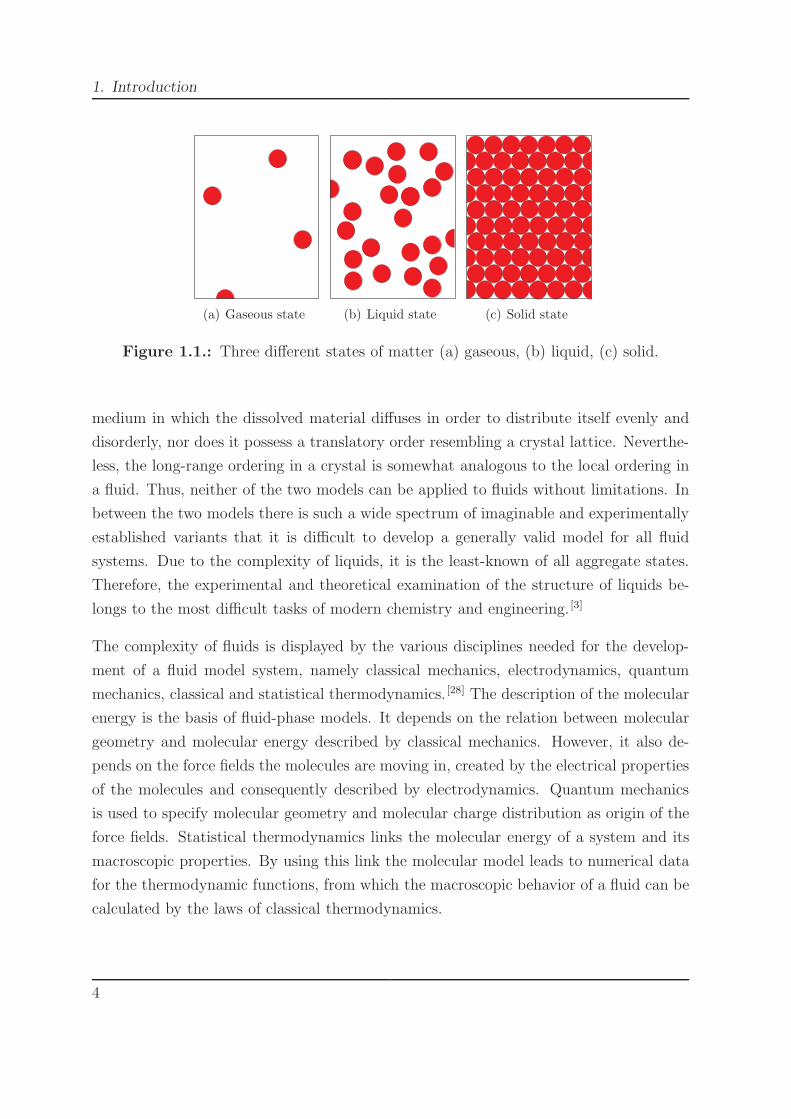
matter, the gaseous, the solid and the liquid (Figure 1.1).
The gas phase is remarkably simple. At low to moderate pressures, molecules may be
treated as isolated, non-interacting species. This facilitates theoretical modeling enor-
mously since the system of interest is entirely defined by the single molecules. [29] In a
solid, on the other hand, molecules are closely packed and their motion is restricted to
small vibrations around space-fixed positions. Thus, a solid is highly ordered. In liquid
systems, the interactions between the molecules are on the one hand too strong to be
treated by the kinetic theory of gases, and on the other hand too weak to be treated by
the laws of solid state physics. Thus, the liquid is neither a microscopically homogeneous
3
1. Introduction
(a) Gaseous state (b) Liquid state (c) Solid state
Figure 1.1.: Three different states of matter (a) gaseous, (b) liquid, (c) solid.
medium in which the dissolved material diffuses in order to distribute itself evenly and
disorderly, nor does it possess a translatory order resembling a crystal lattice. Neverthe-
less, the long-range ordering in a crystal is somewhat analogous to the local ordering in
a fluid. Thus, neither of the two models can be applied to fluids without limitations. In
between the two models there is such a wide spectrum of imaginable and experimentally
established variants that it is difficult to develop a generally valid model for all fluid
systems. Due to the complexity of liquids, it is the least-known of all aggregate states.
Therefore, the experimental and theoretical examination of the structure of liquids be-
longs to the most difficult tasks of modern chemistry and engineering. [3]
The complexity of fluids is displayed by the various disciplines needed for the develop-
ment of a fluid model system, namely classical mechanics, electrodynamics, quantum
mechanics, classical and statistical thermodynamics. [28] The description of the molecular
energy is the basis of fluid-phase models. It depends on the relation between molecular
geometry and molecular energy described by classical mechanics. However, it also de-
pends on the force fields the molecules are moving in, created by the electrical properties
of the molecules and consequently described by electrodynamics. Quantum mechanics
is used to specify molecular geometry and molecular charge distribution as origin of the
force fields. Statistical thermodynamics links the molecular energy of a system and its
macroscopic properties. By using this link the molecular model leads to numerical data
for the thermodynamic functions, from which the macroscopic behavior of a fluid can be
calculated by the laws of classical thermodynamics.
4

1.2. Molecular models for fluid phases
1.2.2. Inter- and intramolecular potential energy
For a single molecule, the energy can be expressed in terms of its mechanical degrees
of freedom. The energy can be calculated out of the molecular geometry, represented
by various moments of inertia, the atomic masses and the properties related to the
intramolecular force fields, such as vibration frequencies and the barriers to internal
rotation. The energy of a single molecule constitutes one part of the total energy of a
molecular system, referred to as the kinetic part. Molecules have a potential part that
needs to be considered as well if different conformers exist or reactions occur.
Defining a fluid, a potential part is added, originating from the intermolecular potential
energy of a molecular system. In general, all degrees of freedom such as translation,
rotation and internal motions will be influenced by adjacent molecules. This interaction
with the molecular environment can be expressed in terms of the forces acting between
the molecules, which in turn are derived from the intermolecular potential energy. So,
although the simple equations for the kinetic energies associated with the various degrees
of freedom continue to be valid, they have to be supplemented by an expression for the
intermolecular potential energy in terms of the molecular configuration of the system.
1.2.3. Fundamental equations
The most fundamental equations of thermodynamics are the first and the second law of
thermodynamics. A combination of these equations leads to a thermodynamic relation
that generally describes all thermodynamic properties of a system. For a defined system
this fundamental thermodynamic relation may be expressed in terms of the internal
energy:
dU(S, V, Ni) = TdS − pdV +∑
i
µidNi. (1.1)
Using the Legendre transform, this fundamental thermodynamic equation for the internal
energy can be transformed into fundamental equations for additional thermodynamic
potentials. Hence, in addition to the internal energy the most important fundamental
5
1. Introduction
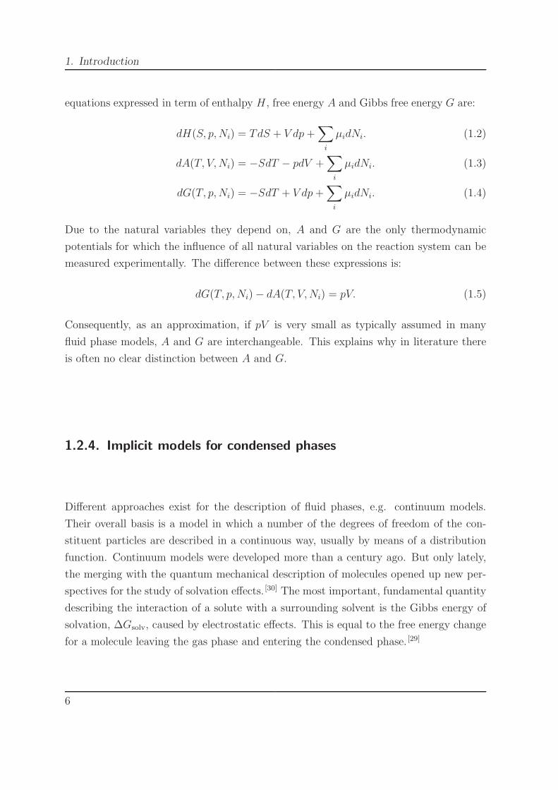
equations expressed in term of enthalpy H , free energy A and Gibbs free energy G are:
dH(S, p, Ni) = TdS + V dp +∑
i
µidNi. (1.2)
dA(T, V, Ni) = −SdT − pdV +∑
i
µidNi. (1.3)
dG(T, p, Ni) = −SdT + V dp +∑
i
µidNi. (1.4)
Due to the natural variables they depend on, A and G are the only thermodynamic
potentials for which the influence of all natural variables on the reaction system can be
measured experimentally. The difference between these expressions is:
dG(T, p, Ni) − dA(T, V, Ni) = pV. (1.5)
Consequently, as an approximation, if pV is very small as typically assumed in many
fluid phase models, A and G are interchangeable. This explains why in literature there
is often no clear distinction between A and G.
1.2.4. Implicit models for condensed phases
Different approaches exist for the description of fluid phases, e.g. continuum models.
Their overall basis is a model in which a number of the degrees of freedom of the con-
stituent particles are described in a continuous way, usually by means of a distribution
function. Continuum models were developed more than a century ago. But only lately,
the merging with the quantum mechanical description of molecules opened up new per-
spectives for the study of solvation effects. [30] The most important, fundamental quantity
describing the interaction of a solute with a surrounding solvent is the Gibbs energy of
solvation, ∆Gsolv, caused by electrostatic effects. This is equal to the free energy change
for a molecule leaving the gas phase and entering the condensed phase. [29]
6
1.2. Molecular models for fluid phases
1.2.4.1. Continuum solvation models
Continuum models differ in the way they describe the degrees of freedom of the con-
stituent particles in a continuous way. One approach is to neglect the atomic structure
of the solvent and replace its electrostatic properties by those of a dielectric continuum.
The polarization of the medium and the back-polarization of the solute are the elec-
trostatic response to placing the solute molecule in the solvent and thus a measure of
the electrostatic interactions between solvent and solute. The macroscopic effect of this
electrostatic interaction energy is calculated by a particular branch of continuum models,
referred to as continuum solvation models. Since the first application of this approach, [31]
many different versions of the model have appeared. [30,32–34] They all have in common
that a cavity is constructed that represents the geometry of the solute molecule and
that the solvent is represented by an infinitely extended dielectric continuum outside
this cavity. The electric field, arising from the nuclei as well as from the electrons of
the solute molecule, is screened by the polarization of this continuum. The effect of this
polarization can be represented by the surface charge density distribution it produces on
the inner surface of the cavity. Also, the screening charges back-polarize the solute and
thus change its charge distribution. In a continuum solvation model the electrostatic
interactions between solute and solvent molecules in a real solution, resulting from the
interactions between the the molecular charge densities, are thus modeled by a rather
localized system, the charges of the solute in the solvent interacting with the associated
charged surface of the cavity. [29]
1.2.4.2. Quantum mechanics
The starting point for the calculation of thermodynamic properties using modern con-
tinuum solvation models is in each case quantum mechanics which is used to calculate a
large variety of molecular properties of isolated molecules in vacuo. The ultimate goal of
most quantum chemical approaches is to find a solution of the time-independent, non-
relativistic Schrodinger equation. This differential equation cannot be solved analytically
for more than one-electron systems. Furthermore, the direct numerical integration is not
tractable. As a result, a large number of approximate methods have evolved to solve
7

1. Introduction
the Schrodinger equation, for example electronic structure methods, electron correlation
methods and density functional theory.
One of the most basic theories is the Hartree-Fock (HF) theory, [35–37] an electronic struc-
ture method where electron correlation is neglected. This approximation is the corner-
stone of almost all conventional orbital based quantum chemical methods. The under-
lying molecular orbital picture was, and still is, the most important theoretical concept
for the interpretation of reactivity and molecular properties.
A further development are electron correlation methods that consequently lead to more
accurate results, usually at higher computational costs. Here, most widely used electron
correlation methods are the Møller-Plesset perturbation theory of nth order (MPn), [38]
and the coupled cluster theory (CC). [39,40] In the MPn theory the perturbation theory is
applied to the calculation of the correlation energy. The most frequently used variations
are MP2 [41–44] and MP4. [45] Perturbation methods add all types of corrections to a given
order, whereas coupled cluster (CC) methods include all corrections of a given type to
infinite order. [46] An important variation is CCSD(T) (coupled cluster with single and
double excitations and perturbative triple excitations). [47,48]
A completely different approach to quantum chemistry in comparison to the mentioned
orbital based methods with or without electron correlation is the density functional
theory (DFT). [49,50] Instead of working with wavefunctions, DFT makes use of the elec-
tron density as fundamental variable because Hohenberg and Kohn could prove that
the ground-state electronic energy is completely determined by the electron density. [50]
Hence, DFT methods utilize empirical functionals connecting electron density and en-
ergy. DFT is a ground state theory that incorporates both exchange and correlation
effects. Among the different methods that exist within density functional theory, hybrid
methods such as B3LYP (Becke three parameter hybrid functional) are commonly used
due to its good accuracy and computational economy.
Quantum chemical methods allow a calculation of thermodynamic properties of molecules
in the gas phase, depending on the method of choice with more or less accurate results.
To move from the quantum mechanic prediction of gas phase properties to fluid-phase
properties, continuum solvation models are useful tools.
8
1.2. Molecular models for fluid phases
1.2.4.3. COSMO
Among continuum solvation models in literature, one is of particular practical usefulness,
namely COSMO (conductor-like screening model). In this model, the continuum chosen
to represent the solvent is an infinitely extended electrical conductor with ǫ → ∞. [51]
This choice leads to a remarkably simple expression for the screening charges and the
screening energy, because the resulting electrostatic potential Φ is zero for every point r
on the surface of the cavity in the conductor:
Φ(r) = 0. (1.6)
Because the electrical conductor screens the charges perfectly, it is intuitively clear that
all electrostatic effects vanish behind the electrically conducting surface, including the
electrostatic potential. The disadvantage using this assumption is that it is only exact
for a molecule in a conductor, not for a solvent with a finite dielectric constant ǫ. An
approximate correction for non-conducting media offers the approach to scale the ideal
screening charge densities σ∗:
σ = f(ǫ)σ∗ =ǫ − 1
ǫ + xσ∗. (1.7)
For many problems, x can be calculated exactly, it is always 0 ≤ x ≤ 2. For COSMO x =12
was chosen, the relative error is less than 12ǫ. Some concerns were raised initially that
this post facto correction for the dielectric behavior is only appropriate for media having
reasonably high dielectric constants (such as water), but a systematic study indicated
non-polar solvents to be equally amenable to a treatment by the COSMO model. [29,52]
Since its original description at semi-empirical level, COSMO has been generalized to ab
initio and density functional levels of theory as well. [53]
An important point is the construction of the cavity around the solute. In COSMO,
the cavities are constructed by modeling a solute molecule by a fused sphere geometry
and choosing the radii as the spheres representing the atoms by fitting to experimental
data; quite common is the use of 1.2 times the corresponding van der Waals radii. [54]
Furthermore, the segmentation of the cavity surface must be done properly for reliable re-
sults. In a practical COSMO calculation the number of surface segments typically ranges
9
1. Introduction
from about one hundred for diatomic molecules to a few thousand for drug molecules.
COSMO calculations have been incorporated into various quantum-chemical computer
packages, so that the results can be generated without bothering about every detail of
their production. [54] The thermodynamic energy of solvation obtained from COSMO will
in general be no more than a crude approximation of the true experimental value. This
is to be expected because the macroscopic dielectric constant cannot accurately repro-
duce the local electrostatic interactions between solute and solvent molecule. Results of
a COSMO calculation are the charge density distribution over the surface of the cavity
and the energy of the solute in the conductor, including the back-polarization effect. The
difference between the energy of the solute in the conductor and in the gas phase reflects
the electrostatic intermolecular interactions. It is not a molecular potential energy, but
rather has been shown to be approximate to the electrostatic part of the thermodynamic
free energy of solvation.
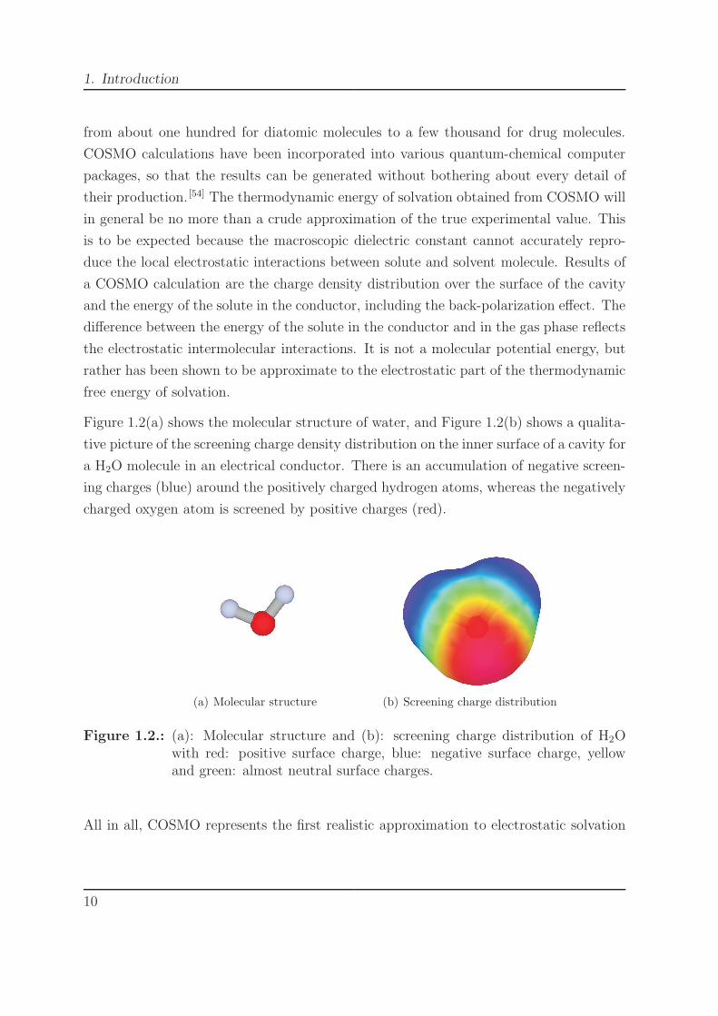
Figure 1.2(a) shows the molecular structure of water, and Figure 1.2(b) shows a qualita-
tive picture of the screening charge density distribution on the inner surface of a cavity for
a H2O molecule in an electrical conductor. There is an accumulation of negative screen-
ing charges (blue) around the positively charged hydrogen atoms, whereas the negatively
charged oxygen atom is screened by positive charges (red).
(a) Molecular structure (b) Screening charge distribution
Figure 1.2.: (a): Molecular structure and (b): screening charge distribution of H2Owith red: positive surface charge, blue: negative surface charge, yellowand green: almost neutral surface charges.
All in all, COSMO represents the first realistic approximation to electrostatic solvation
10
1.2. Molecular models for fluid phases
effects. Although not generally reliable or sufficiently accurate, it is a good starting point
for a realistic semi-empirical model of the molecular potential energy in liquid mixtures
beyond the continuum solvation approximation.
1.2.5. Excess function models
Moving beyond computation of the electrostatic component of the solvation free energy,
excess function models are used to describe properties of liquid mixtures with reference
to the pure component properties. But due to the complexity of liquids, liquid models
are used for a simplified treatment of mixing effects.
1.2.5.1. Basics of excess function models
Any molecular model for the excess free energy AE is made up of two separate contribu-
tions, a repulsive AErep and an attractive AE
att:
AE = AErep + AE
att. (1.8)
The repulsive term accounts for molecular size and shape effects, hence it introduces
the molecular geometry. The attractive part is associated with attractive intermolec-
ular forces. Since mixing effects of industrially relevant systems usually occur at high
densities, a reasonable approximation is that the molecular system is represented by a
space-filling arrangement of molecules interacting via surface contacts. This crude ap-
proximation implies that pressure-dependent effects cannot be calculated using these
simplified liquids models. In addition, a distance dependency is suppressed which means
that only temperature dependencies can be taken into consideration. Because the in-
termolecular interactions are formulated in terms of pair contacts, they will depend on
the local structure in the liquid. Thus, an essential part of any molecular model for the
excess functions in liquid mixtures is a model for the relation between the unknown local
compositions and the known bulk compositions in terms of the intermolecular potential
energy, hence the short-range non-randomness (Figure 1.3).
11

1. Introduction
Figure 1.3.: The concept of local composition: Although the bulk composition of redand black balls is 1:1, the local compositions, exemplary accentuated bygray circles, differ.
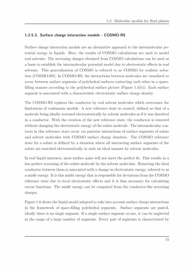
Nevertheless, simplified liquid models are useful representations of the intermolecular
potential energy of fluid phases. Two different approaches will be presented (Figure 1.4),
group interaction models based on the lattice picture (Figure 1.4(a)) and surface charge
interaction models based on the polyhedral surface picture (Figure 1.4(b)).
1.2.5.2. Group interaction models - UNIFAC
Group interaction models are based on the liquid model in the lattice picture as shown
in Figure 1.4(a). They calculate the intermolecular energy as the sum of independently
interacting functional groups according to the free segment approximation. At present,
UNIFAC is one of the most popular group interaction models. [55,56] The functionality
of UNIFAC is exemplary shown in Figure 1.5 for a mixture of hexane and butanone.
Both molecules are broken up into their functional groups; hexane is broken up into
-CH2 and -CH3, and butanone is broken up into -CH3, -CH2 and -COCH3. This leads
to specific group frequencies for the pure components. The intermolecular energy in
the mixture is calculated from a summation over all pair contact energies between the
different functional groups in the mixture. The interaction energies cannot be calculated
yet from quantum mechanics and hence must be determined by fitting to experimental
12
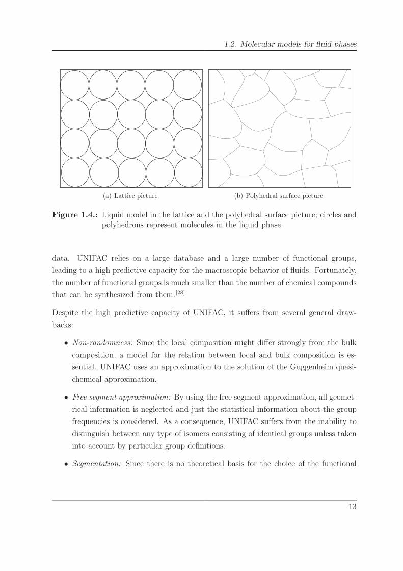
1.2. Molecular models for fluid phases
(a) Lattice picture (b) Polyhedral surface picture
Figure 1.4.: Liquid model in the lattice and the polyhedral surface picture; circles andpolyhedrons represent molecules in the liquid phase.
data. UNIFAC relies on a large database and a large number of functional groups,
leading to a high predictive capacity for the macroscopic behavior of fluids. Fortunately,
the number of functional groups is much smaller than the number of chemical compounds
that can be synthesized from them. [28]
Despite the high predictive capacity of UNIFAC, it suffers from several general draw-
backs:
• Non-randomness: Since the local composition might differ strongly from the bulk
composition, a model for the relation between local and bulk composition is es-
sential. UNIFAC uses an approximation to the solution of the Guggenheim quasi-
chemical approximation.
• Free segment approximation: By using the free segment approximation, all geomet-
rical information is neglected and just the statistical information about the group
frequencies is considered. As a consequence, UNIFAC suffers from the inability to
distinguish between any type of isomers consisting of identical groups unless taken
into account by particular group definitions.
• Segmentation: Since there is no theoretical basis for the choice of the functional
13

1. Introduction
butanone
equimolar mixture
1/3 1/3 1/3
CH -CH -COCH3 2 3
n-hexane
1/3 1/3
CH -CH -CH3 2 3-CH -CH -CH2 2 2
1/9
5/9
1/31/31/31/3
3/9
3/9
-COCH3-C -H2C -H3
Figure 1.5.: Frequency profile of functional groups in the 1:1 mixture of butanone andhexane. [28]
groups, different scientific groups might use different segmentations and conse-
quently yield different results.
• Parameterization: Since the interaction energies between different functional groups
cannot yet be calculated using quantum mechanics, UNIFAC depends on experi-
mental data for these values. Consequently, it is only applicable for molecules that
consist of already parameterized groups.
• Temperature dependency: With the original basic UNIFAC, no temperature de-
pendency could be considered; the parameters needed to be fitted to experimental
data. Newer, modified UNIFAC versions, as usually used today, can take temper-
ature dependent parameters into account. [57]
In summary, a group contribution method like UNIFAC is a highly predictive method for
fluid-phase behavior of molecules whose functional groups have already been parameter-
ized. It does not, however, represent a realistic picture of the intermolecular interaction
resulting from the surface properties of the molecule.
14
1.2. Molecular models for fluid phases
1.2.5.3. Surface charge interaction models - COSMO-RS
Surface charge interaction models are an alternative approach to the intermolecular po-
tential energy in liquids. Here, the results of COSMO calculations are used to model
real solvents. The screening charges obtained from COSMO calculations can be used as
a basis to establish the intermolecular potential model due to electrostatic effects in real
solvents. This generalization of COSMO is referred to as COSMO for realistic solva-
tion (COSMO-RS). In COSMO-RS, the interactions between molecules are visualized to
occur between surface segments of polyhedral surfaces contacting each other in a space-
filling manner according to the polyhedral surface picture (Figure 1.4(b)). Each surface
segment is associated with a characteristic electrostatic surface charge density.
The COSMO-RS replaces the conductor by real solvent molecules which overcomes the
limitations of continuum models. A new reference state is created, defined as that of a
molecule being ideally screened electrostatically by solvent molecules as if it was dissolved
in a conductor. With the creation of the new reference state, the conductor is removed
without changing the electrostatic energy of the solute molecule. The intermolecular con-
tacts in this reference state occur via pairwise interactions of surface segments of solute
and solvent molecules with COSMO surface charge densities. The COSMO reference
state for a solute is defined by a situation where all interacting surface segments of the
solute are matched electrostatically in such an ideal manner by solvent molecules.
In real liquid mixtures, most surface pairs will not meet the perfect fit. This results in a
less perfect screening of the solute molecule by the solvent molecules. Removing the ideal
conductor between them is associated with a change in electrostatic energy, referred to as
a misfit energy. It is this misfit energy that is responsible for deviations from the COSMO
reference state due to local electrostatic effects and it is thus necessary for calculating
excess functions. The misfit energy can be computed from the conductor-like screening
charges.
Figure 1.6 shows the liquid model adapted to take into account surface charge interactions
in the framework of space-filling polyhedral segments. Surface segments are paired,
ideally there is no single segment. If a single surface segment occurs, it can be neglected
in the range of a large number of segments. Every pair of segments is characterized by
15

1. Introduction
the surface area of a segment aeff and the total surface charge density σtot. The latter is
the sum of the local screening charge densities, σtot = σ + σ′. When σ = −σ′ it is called
an ideal contact. With σ 6= −σ′ the screening charge densities do not cancel out and the
energy of this non-ideal pair is called misfit energy :
Emisfit(σ, σ′) = aeffα
2(σ + σ′)2, (1.9)
where α is an electrostatic misfit energy coefficient for converting a charge into an energy,
and aeff, the surface area of the segment, transforms the charge densities into charges.
Both are adjustable parameters of the model.
Figure 1.6.: COSMO-RS interaction model.
Although local electrostatic effects in the fluid are quite well modeled by the misfit energy,
there will be further contributions of electrostatic origin to the intermolecular potential
energy of liquids. If the absolute values of the screening charge densities of two interacting
surface segments are large enough and of opposite sign, an energy contribution to the
description of hydrogen bonds has to be considered:
Ehb = aeffchb max[0, σacc − σhb] min[0, σdon + σhb] (1.10)
where σhb and chb are fitted parameters.
To move from mixtures of segments to real solvent, a crucial simplification is possible by
16

1.2. Molecular models for fluid phases
invoking the free segment approximation. Then, the geometrical information contained
in the COSMO files is irrelevant and statistical information about the frequencies of
particular charge densities in a molecule, the so-called σ-profiles, is sufficient. The σ-
profile of a molecule is obtained by a suitable statistical averaging of the charge density
distribution over the effective contact areas. It is basically a histogram in which discrete
σ-values are related to associated surface areas.
The σ-profiles are useful tools to gain qualitative insight into a molecular system. Fig-
ure 1.7 exemplary shows the σ-profiles of water, hexane, toluene and benzene. The
σ-profile of water is very broad which reflects its strongly polar character. Furthermore,
the σ-profile is almost symmetrical, which means that the negative peak of the σ-profile
results in almost ideal screening of the positive peak. Hence, water molecules are not
likely to form non-ideal pairs and the surface segments have a high affinity to each other.
As a consequence, water has a rather high boiling point. In contrast, hexane has a
σ-profile which is rather narrow but high. Due to the differences in the σ-profiles it is
obvious that water and hexane do not show a high miscibility. In contrast, benzene and
toluene show a high mutual solubility represented by their similar σ-profiles. [28]
Continuing with the transformation of the molecule concentrations to segment concen-
trations, the σ-profile of a whole system Ps(σ) is the sum of the mole fraction weighted
σ-profile of all components:
Ps(σ) =∑
xiP′(σ). (1.11)
The chemical potential of a segment is given by the following equation which has to be
solved iteratively:
µs(σ) = −RT
aeff
[∫
Ps(σ′) exp
( aeff
RT(µs(σ
′) − Emisfit(σ, σ′) − Ehb(σ, σ′)))
dσ′
]
. (1.12)
The move from a segment to molecules is described by the following equation, which
assembles the chemical potential of a component i in a solvent S by a combinatorial
term and a residual term
µis = µi
c,S + µires,S = µi
c,S +
∫
P ′(σ)µs(σ)dσ. (1.13)
17

1. Introduction
0
2
4
6
8
10
12
14
16
18
20
22
24
0
s [e/nm ]2
water
toluene
benzene
hexane
P[-
](s
)
0.5 1.0 1.5 2.0 2.5 3.00.51.01.52.02.53.0
Figure 1.7.: σ-profiles of different molecules.
The combinatorial term µic,S takes shape and size effects of solvent molecules and solvate
molecules into account. The residual term µires,S describes the interactions between solvate
i and solvent S.
For each molecule, a quantum chemical geometry optimization combined with a COSMO
calculation has to be carried out just once. These calculations can usually be done
overnight on a single CPU, but they might get time-consuming when moving to molecules
with more than 100 atoms. The results can be stored in a database for further use. Note
that a conformer analysis is important because it can lead to energetic changes. The sub-
sequent COSMO-RS calculations using a statistical thermodynamics approach, leading
to the prediction of thermodynamic properties such as excess Gibbs energies and parti-
tion coefficients, only take a few seconds. Consequently, COSMO-RS is a valuable tool
for screening purposes, e.g. for a solvent screening using a solvent database. The overall
18

1.2. Molecular models for fluid phases
workflow of the calculation of mixture equilibrium data is illustrated in Figure 1.8.
Figure 1.8.: Workflow of the calculation of mixture equilibrium data.
Nevertheless, COSMO-RS has several disadvantages that limit a general applicability.
• No density dependence: Being a simplified liquid model based on the polyhedral
surface interactions, COSMO-RS approximates the molecules in a liquid to be
densely packed. Consequently, it is not possible to calculate pressure dependencies.
• Non-randomness: For the relation between bulk and local composition, COSMO-
RS uses an iterative solution to the quasi-chemical approximation of Guggen-
heim; the iterative solution is identical with the one used in other models, such
as GEQUAC.
• Free segment approximation: A crucial simplification within COSMO-RS is the
use of the free segment approximation. The geometrical information is neglected
19
1. Introduction
and just the statistical information about the frequencies of the screening charge
densities are important, the so-called σ-profiles. By this, COSMO-RS cannot dis-
tinguish stereoisomers. But in contrast to UNIFAC, a discrimination of structural
isomers is possible (e.g. ethanol and dimethylether).
• Dissociation: The tendency of molecules to dissociate cannot automatically be
covered by COSMO-RS.
In the future, predictive models based on polyhedral surface charge distributions will play
an important role for the prediction of mixture equilibrium data. Due to an increasing
computer power, these methods are likely to become one of the most important branches
of progress. At present, highly parameterized group contribution methods are often more
accurate. [28]
1.3. Applications of fluid-phase models
Due to their predictive power, fluid-phase models are widely applied in the chemical
industry. For COSMO-RS and UNIFAC, chemical engineering simulations have become
the most important area of applications. Both are often used as thermodynamic models
in process simulations. COSMO-RS is also commonly applied by the pharmaceutical
industry for drug development or direct product design. UNIFAC as well as COSMO-RS
are used for industrial solvent screenings.
Fluid phase models are also used in algorithms, such as in the computer-aided molecular
design (CAMD) approach. [58] Here, up to date, UNIFAC and further developments of
UNIFAC are used for the prediction of pure compound and mixture properties. [59] In
addition to that, the CAMD approach also screens for intrinsic molecular properties such
as melting point, boiling point or toxicity. All these parameters are also important for
the choice of suitable solvent combinations. The method still suffers from disadvantages:
apart from the general problems of group contribution methods, the CAMD approach
does not take molecular conformations into account up to date. Regardless, the CAMD
approach is a valuable tool for a fast and effective industrial solvent selection.
20
1.4. Objective
In general, for a more sophisticated prediction of fluid-phase properties, equations of state
(EOS) are used. [60] Especially, if the fluid phase over a large region of pressure or density
is considered, excess function models are no longer applicable. In theory, an equation of
state model is generally applicable and does not have theory based limitations like excess
function models. Nevertheless, in practice, a generally applicable equation of state has
not yet been found. Specific EOS are used for specific applications. Although equations
of state are computationally more demanding than excess function models, they are at
the same time very accurate if not correlative.
For an even more sophisticated investigation of fluid phases, Molecular Dynamics [61,62]
or Monte-Carlo Methods [63,64] can be used. Both rely on the availability of suitable force
fields. They lead to highly accurate results if appropriate force-field are available at high
computational costs. But up to date, computers are not fast enough for an efficient use
of these methods for everyday problems in the chemical and pharmaceutical industry.
1.4. Objective
To use biphasic reaction conditions effectively, a distinct knowledge of the equilibrium
thermodynamic boundaries is of great value. In order to obtain reliable data, a large
number of time-consuming and expensive experiments is necessary. To minimize the
amount of experimental work but also to reduce the environmental impact, a computa-
tional approach to solvent selection according to maximum equilibrium conversion and
product yield is proposed as depicted in Figure 1.9.
The first step in a computational solvent selection is the selection of a target reaction
system as discussed in Chapter 2. The reaction system examined is a biphasic reaction
system with only one reactive phase. For the idealized reaction system, an analytical
solution is derived in order to calculate and predict equilibrium conversion and product
yield.
In the second step, a suitable target reaction is chosen. Biocatalytic reactions are good
model reactions for biphasic reaction systems with one reactive phase as they offer the
advantages of ideal product selectivity and a strong thermodynamic limitation. Two
21

1. Introduction
gPROMS
COSMO-RS
target reaction,target reaction system optimized system
experimentalverification
materialdata
reaction system
phase equilibrium:partition coefficients
reaction equilibrium:Gibbs free energies
analyticalsolution
numericalsimulation
Figure 1.9.: Computational approach to solvent selection.
biocatalytic reactions are examined here: The first reaction is an enantioselective sub-
strate coupled cofactor regeneration where acetophenone is reduced to (R)-phenylethanol
while 2-propanol is oxidized to acetone. The catalyst used is an alcohol dehydrogenase
from Lactobacillus brevis (LB -ADH). The second reaction is the enantioselective carbon-
carbon coupling of 3,5-dimethoxy-benzaldehyde (DMBA) to (R)-3,3’,5,5’-tetramethoxy-
benzoin (TMB) using the enzyme benzaldehyde lyase (BAL).
For the selected target reactions, material-specific data needs to be collected such as par-
tition coefficients and equilibrium constants. In Chapter 3, the calculation of partition
coefficients using the conductor-like screening model for real solvents (COSMO-RS) is
discussed. This method is used because it offers the possibility of an ab initio prediction
of the phase equilibria. Moreover, a method for the ab initio prediction of equilibrium
constants using a combination of quantum mechanics and statistical thermodynamics is
the topic of Chapter 4. Subsequent to that, the calculated material data needs to be
inserted into the mathematical model derived in Chapter 2.
22

1.4. Objective
The last step in the computational solvent screening is an experimental validation. Calcu-
lated and experimentally obtained conversion and yield of the target reaction in different
solvent combinations are compared. Finally, the optimal solvent in terms of equilibrium
conversion and product yield for the target reaction in an idealized target reaction system
can be identified. This is shown throughout the thesis in Chapter 2 - Chapter 5.
Apart from conversion and yield, there are of course many more parameters that deter-
mine an optimal solvent, e.g. price, toxicity, temperature dependence, long-term stability.
The computational screening for maximum equilibrium conversion and product yield is
meant to be a starting point for a final solvent selection. For a more detailed study of
the reaction system, a further investigation of the target reaction system using numerical
simulation tools is of great value as presented in Chapter 5.
23

1. Introduction
24

2. Mathematical analysis of biphasic
reaction systems
2.1. Introduction
Various parameters determine the choice of a suitable solvent, such as enantiomeric
excess, toxicity, long-term stability, price and so forth. From a practical point of view,
conversion and yield are important targets for process optimization. Consequently, within
this thesis, these are the parameters chosen to determine a suitable solvent.
For an ab initio prediction of conversion and yield in biphasic systems, the first step is
a mathematical analysis of the thermodynamic equilibrium. Subsequently a parameter
study and a sensitivity analysis will be carried out. Finally, the validity of the derived
model will be tested in an experimental validation.
2.2. Materials and methods
2.2.1. Computational
Algebraic transformations were carried out using Maple 10 (The Mathworks). Graphs
have been created using PSTricks. All calculations were performed by the author of this
thesis.
25

2. Mathematical analysis of biphasic reaction systems
2.2.2. Experimental
All experiments were carried out by M. Eckstein as part of her PhD thesis [65] and by
Julia Lembrecht (both Technical Chemistry, University of Rostock, Germany) as part of
her diploma thesis. Experimental details are described elsewhere. [66,67]
2.3. Results and discussion
A general reaction scheme, which applies to the majority of reactions in biphasic systems,
is the bimolecular reversible reaction with partitioning of all reactants (Figure 2.1). The
catalyst is restricted quantitatively to the reactive phase (index: R). The second phase
acts as a reservoir for the reactants and the extracted products and is thus defined as
non-reactive phase (index: N). For a detailed description of equilibrium conversion X
and yield η, seven different parameters have to be taken into account:
• partition coefficients α, β, γ, δ
• phase volume ratio V = VN
VR
• co-substrate excess S = n(B)0n(A)0
• equilibrium constant K.
AN
BN
CN
DN
+AN
BN
CN
DN
+
VN
VR
a b g d
K
catalyst
Figure 2.1.: Bimolecular reaction with partitioning of all reactants; A and B are thesubstrates, C and D the products; indices R and N indicate reactive andnon-reactive phase, respectively; K is the equilibrium constant; V is thephase volume ratio; α, β, γ, δ are the partition coefficients.
26

2.3. Results and discussion
The whole system was idealized in order to identify the general underlying trends. The
partition coefficients express the reactant’s affinity to the non-reactive phase. The par-
tition coefficient of compound A is given by the ratio of the concentration of compound
A in the reactive phase [A]R and in the non-reactive phase [A]N as α = [A]N
[A]R, with β, γ,
and δ accordingly. Partition coefficients were regarded as constant and independent of
each other. Activity coefficients and selectivity were set to unity. Initially, no products
were present. Selectivity towards the products was taken as unity.
2.3.1. Mathematical description
For the idealized system an analytical expression describing the thermodynamic conver-
sion X of a bimolecular reaction with partitioning of all reactants in a biphasic system
as a function of the seven previously mentioned parameters was derived. A closed solu-
tion for the recoverable, thus technically relevant, amount of product in the non-reactive
phase expressed as yield η was also derived. By this, the values can be calculated di-
rectly avoiding numerical simulations. Furthermore, with the analytical solutions at
hand, derivatives with respect to all the variables are in principle available.
The analytical solution was derived by expressing the conversion of the limiting substrate
A by the molar amounts n(A) and n(C)
X :=n(A)0 − n(A)
n(A)0=
n(C)
n(A)0(2.1)
with the initial total molar amount of compound A as n(A)0.
The equilibrium constant K is given by the mass action law and in the idealized system
by the ratio of the concentrations of all reactants in the reactive phase
K =[C]R[D]R
[A]R[B]R. (2.2)
27
2. Mathematical analysis of biphasic reaction systems
Applying the relevant mass balance equations
n(A)R + n(A)N = n(A)0 (1 − X) (2.3)
n(B)R + n(B)N = n(A)0 (S − X) (2.4)
n(C)R + n(C)N = n(A)0 X (2.5)
n(D)R + n(D)N = n(A)0 X . (2.6)
The molar amounts of the reactants in the reactive phase are given by the mass balances
n(A)R =n(A)N
αV=
(n(A)0) (1 − X)
(αV + 1)(2.7)
n(B)R =n(B)N
βV=
(n(A)0) (S − X)
(βV + 1)(2.8)
n(C)R =n(C)N
γV=
(n(A)0) X
(γV + 1)(2.9)
n(D)R =n(D)N
δV=
(n(A)0) X
(δV + 1). (2.10)
Thus, the expression the equilibrium constant of the system can be written as
K(γV + 1)
(αV + 1)
(δV + 1)
(βV + 1)=
X2
(1 − X)(S − X). (2.11)
Factor m is defined as factor of the effective concentrations in the reactive phase as
m :=(γV + 1)
(αV + 1)
(δV + 1)
(βV + 1). (2.12)
For single phase systems (V = 0, thus m = 1) equation (2.11) has been solved numeri-
cally [68] as well as analytically. [69] Solving equation (2.11) with respect to X for biphasic
systems with mK 6= 1 gives
X =mK
(
(S + 1) −√
(1 − S)2 + 4S(mK)−1)
2 (mK − 1 ). (2.13)
28
2.3. Results and discussion
Note that for mK = 1 it can be shown that X = S/(1 + S) is the continual completion
in analogy to the monophasic case. [69] Reinsertion of equation 2.12 gives the analytical
expression for the conversion X
X =
(γV +1)(αV +1)
(δV +1)(βV +1)
K
(
(S + 1) −
√
(1 − S)2 + 4S(
(γV +1)(αV +1)
(δV +1)(βV +1)
K)
−1)
2(
(γV +1)(αV +1)
(δV +1)(βV +1)
K − 1) . (2.14)
In practice, the amount of product in the non-reactive phase is of particular interest as
it is equal to the amount of recoverable product. With the mass balance for the desired
product C (equation 2.9) the limiting yield η can be defined as
η =n(C)N
n(A)0=
γV
(γV + 1)X
=
γV (δV +1)(αV +1)(βV +1)
K
(
(S + 1) −√
(1 − S)2 + 4S (mK)−1
)
2 (mK − 1), (2.15)
where γV
(γV +1)is the selectivity factor for the extraction efficiency.
Solving equation 2.11 with respect to S with 0 < X < 1 and 0 < η < 1 gives
S(X) = X
(
1 +
(
1
(X−1 − 1) mK
))
(2.16)
and with rearrangement of equation 2.15
S(η) = η(
1 + (γV )−1)
(
1 +1
η (1 + (γV )−1)mK
)
. (2.17)
This gives S as a function of the desired target variables, thus enabling the calculation
of the initial amounts of substrates needed at minimum to reach a desired value of X
or η. Similar separation of variables to obtain either a solution for V or the partition
coefficients is not possible.
The first and second order derivatives of the equations are complex and reveal no physi-
29
2. Mathematical analysis of biphasic reaction systems
cally reasonable extreme points, neither by direct calculation nor by numerical inspection.
Consequently, a parameter study with the analytical expressions was carried out to show
their influences and interdependencies. The boundaries were chosen to exemplify the gen-
eral trends within physically reasonable limits. In the following sections, the influences
of K, S, V and the partition coefficients α, β, γ, δ on X and η will be discussed.
2.3.2. Equilibrium constant K
The equilibrium constant K is an intrinsic property of the reaction system and is not
easily accessible for optimization. The influence of K follows the intuitive trend that
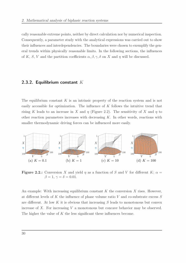
rising K leads to an increase in X and η (Figure 2.2). The sensitivity of X and η to
other reaction parameters increases with decreasing K. In other words, reactions with
smaller thermodynamic driving forces can be influenced more easily.
0V100 S
100
X
η
1
(a) K = 0.10V
100 S100
X
η
1
(b) K = 10V
100 S100
X
η
1
(c) K = 100V
100 S100
X
η
1
(d) K = 100
Figure 2.2.: Conversion X and yield η as a function of S and V for different K; α =β = 1, γ = δ = 0.01.
An example: With increasing equilibrium constant K the conversion X rises. However,
at different levels of K the influence of phase volume ratio V and co-substrate excess S
are different. At low K it is obvious that increasing S leads to monotonous but convex
increase of X. For increasing V a monotonous but concave behavior may be observed.
The higher the value of K the less significant these influences become.
30
2.3. Results and discussion
2.3.3. Partition coefficients α, β, γ, δ
In biphasic reaction systems, many different partition coefficient combinations are possi-
ble. Their influences are complex and interconnected. For the variation of one partition
coefficient at a time, the influence on X and η depends on whether substrates or prod-
ucts are considered: An increase of α or β decreases X and η while, opposite to that, an
increase of γ or δ increases X and η.
However, the independence of partition coefficients is an unlikely scenario. In the major-
ity of catalytic reactions, changes in the molecules are small and partition properties are
interconnected. The ratio and absolute values of the partition coefficients dominate the
influence of V . Here, practically relevant cases were chosen which reflect the intercon-
nection of the chemical nature of the reactants and which demonstrate general trends.
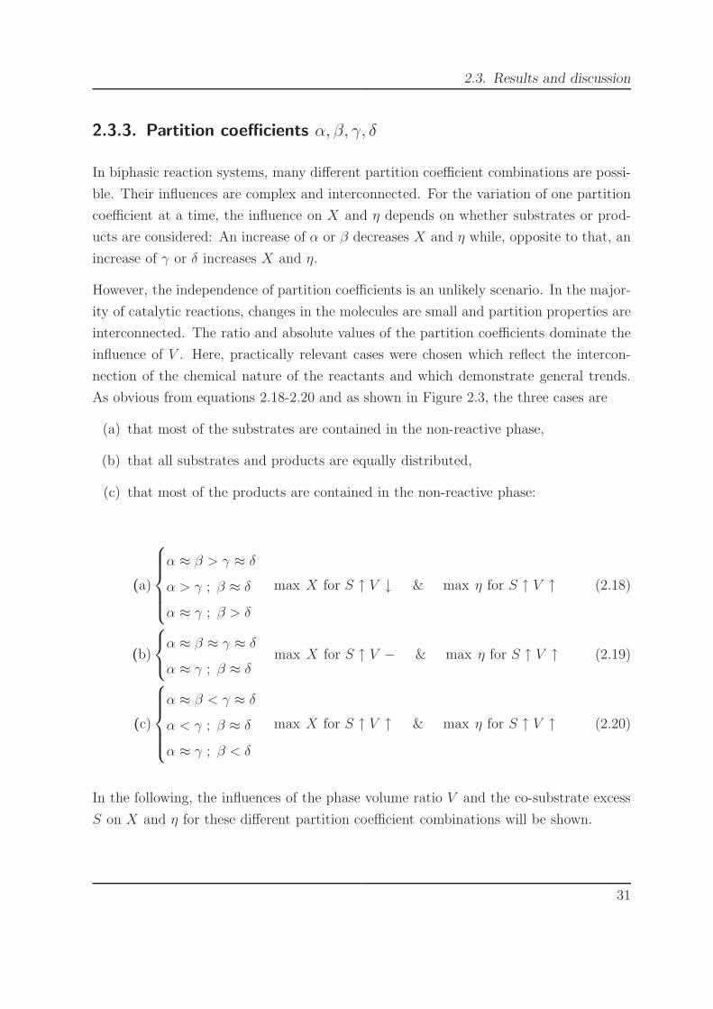
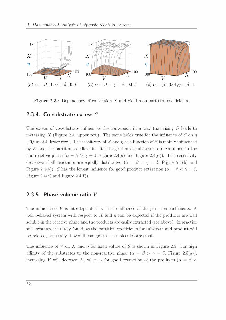
As obvious from equations 2.18-2.20 and as shown in Figure 2.3, the three cases are
(a) that most of the substrates are contained in the non-reactive phase,
(b) that all substrates and products are equally distributed,
(c) that most of the products are contained in the non-reactive phase:
(a)
α ≈ β > γ ≈ δ
α > γ ; β ≈ δ
α ≈ γ ; β > δ
max X for S ↑ V ↓ & max η for S ↑ V ↑ (2.18)
(b)
α ≈ β ≈ γ ≈ δ
α ≈ γ ; β ≈ δmax X for S ↑ V − & max η for S ↑ V ↑ (2.19)
(c)
α ≈ β < γ ≈ δ
α < γ ; β ≈ δ
α ≈ γ ; β < δ
max X for S ↑ V ↑ & max η for S ↑ V ↑ (2.20)
In the following, the influences of the phase volume ratio V and the co-substrate excess
S on X and η for these different partition coefficient combinations will be shown.
31
2. Mathematical analysis of biphasic reaction systems
0V100 S
100
X
η
1
(a) α = β=1, γ = δ=0.010V
100 S100
X
η
1
(a) α = β = γ = δ=0.020V
100 S100
X
η
1
(c) α = β=0.01,γ = δ=1
Figure 2.3.: Dependency of conversion X and yield η on partition coefficients.
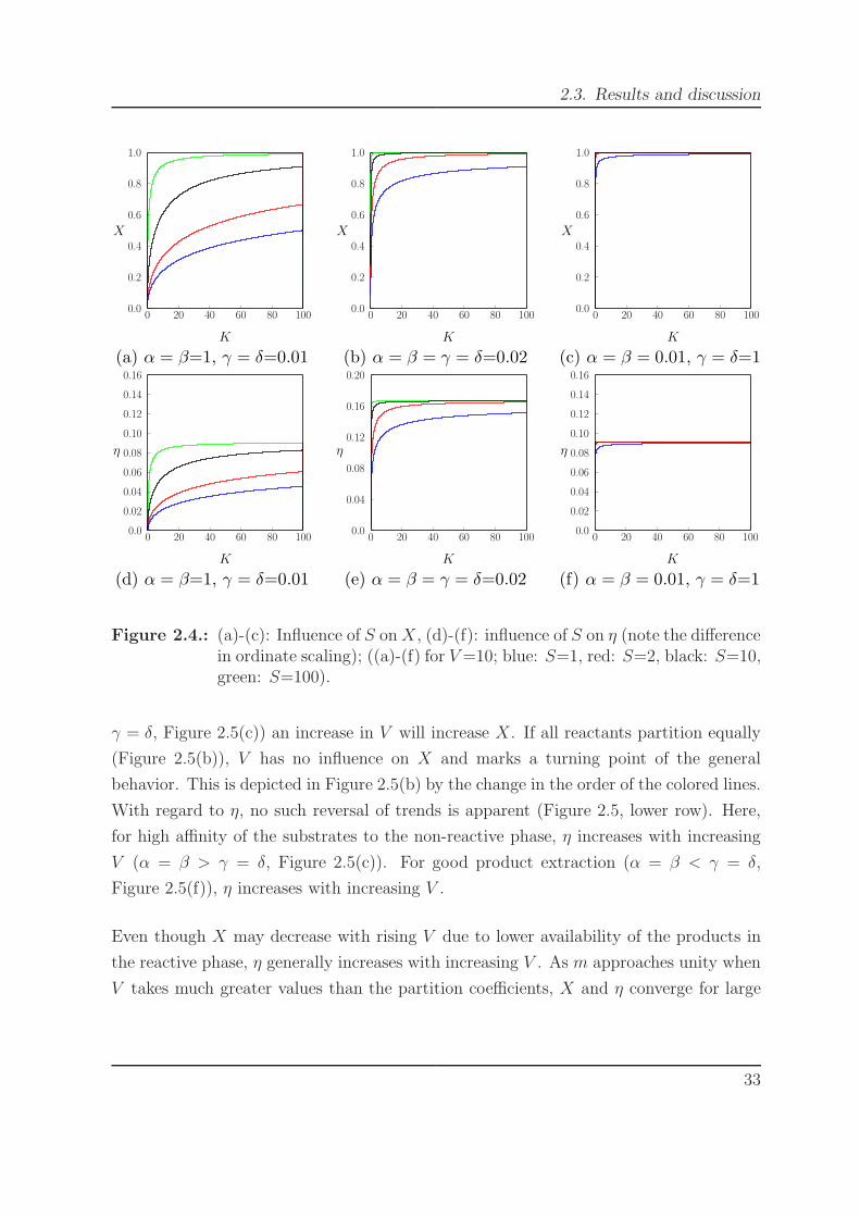
2.3.4. Co-substrate excess S
The excess of co-substrate influences the conversion in a way that rising S leads to
increasing X (Figure 2.4, upper row). The same holds true for the influence of S on η
(Figure 2.4, lower row). The sensitivity of X and η as a function of S is mainly influenced
by K and the partition coefficients. It is large if most substrates are contained in the
non-reactive phase (α = β > γ = δ, Figure 2.4(a) and Figure 2.4(d)). This sensitivity
decreases if all reactants are equally distributed (α = β = γ = δ, Figure 2.4(b) and
Figure 2.4(e)). S has the lowest influence for good product extraction (α = β < γ = δ,
Figure 2.4(c) and Figure 2.4(f)).
2.3.5. Phase volume ratio V
The influence of V is interdependent with the influence of the partition coefficients. A
well behaved system with respect to X and η can be expected if the products are well
soluble in the reactive phase and the products are easily extracted (see above). In practice
such systems are rarely found, as the partition coefficients for substrate and product will
be related, especially if overall changes in the molecules are small.
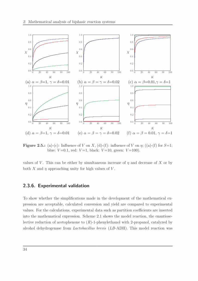
The influence of V on X and η for fixed values of S is shown in Figure 2.5. For high
affinity of the substrates to the non-reactive phase (α = β > γ = δ, Figure 2.5(a)),
increasing V will decrease X, whereas for good extraction of the products (α = β <
32
2.3. Results and discussion
0.0
0.2
0.4
0.6
0.8
1.0
0 20 40 60 80 100
X
K
(a) α = β=1, γ = δ=0.01
0.0
0.2
0.4
0.6
0.8
1.0
0 20 40 60 80 100
X
K
(b) α = β = γ = δ=0.02
0.0
0.2
0.4
0.6
0.8
1.0
0 20 40 60 80 100
X
K
(c) α = β = 0.01, γ = δ=1
0.0
0.02
0.04
0.06
0.08
0.10
0.12
0.14
0.16
0 20 40 60 80 100
η
K
(d) α = β=1, γ = δ=0.01
0.0
0.04
0.08
0.12
0.16
0.20
0 20 40 60 80 100
η
K
(e) α = β = γ = δ=0.02
0.0
0.02
0.04
0.06
0.08
0.10
0.12
0.14
0.16
0 20 40 60 80 100
η
K
(f) α = β = 0.01, γ = δ=1
Figure 2.4.: (a)-(c): Influence of S on X, (d)-(f): influence of S on η (note the differencein ordinate scaling); ((a)-(f) for V =10; blue: S=1, red: S=2, black: S=10,green: S=100).
γ = δ, Figure 2.5(c)) an increase in V will increase X. If all reactants partition equally
(Figure 2.5(b)), V has no influence on X and marks a turning point of the general
behavior. This is depicted in Figure 2.5(b) by the change in the order of the colored lines.
With regard to η, no such reversal of trends is apparent (Figure 2.5, lower row). Here,
for high affinity of the substrates to the non-reactive phase, η increases with increasing
V (α = β > γ = δ, Figure 2.5(c)). For good product extraction (α = β < γ = δ,
Figure 2.5(f)), η increases with increasing V .
Even though X may decrease with rising V due to lower availability of the products in
the reactive phase, η generally increases with increasing V . As m approaches unity when
V takes much greater values than the partition coefficients, X and η converge for large
33
2. Mathematical analysis of biphasic reaction systems
Figure 2.5.: (a)-(c): Influence of V on X, (d)-(f): influence of V on η; ((a)-(f) for S=1;blue: V =0.1, red: V =1, black: V =10, green: V =100).
values of V . This can be either by simultaneous increase of η and decrease of X or by
both X and η approaching unity for high values of V .
2.3.6. Experimental validation
To show whether the simplifications made in the development of the mathematical ex-
pression are acceptable, calculated conversion and yield are compared to experimental
values. For the calculations, experimental data such as partition coefficients are inserted
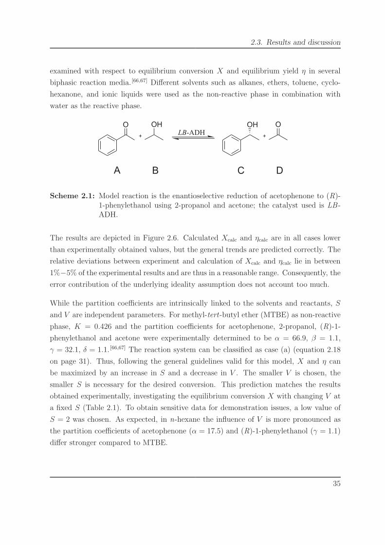
into the mathematical expression. Scheme 2.1 shows the model reaction, the enantiose-
lective reduction of acetophenone to (R)-1-phenylethanol with 2-propanol, catalyzed by
alcohol dehydrogenase from Lactobacillus brevis (LB -ADH). This model reaction was
34
2.3. Results and discussion
examined with respect to equilibrium conversion X and equilibrium yield η in several
biphasic reaction media. [66,67] Different solvents such as alkanes, ethers, toluene, cyclo-
hexanone, and ionic liquids were used as the non-reactive phase in combination with
water as the reactive phase.
O OH
+
OH O
+LB-ADH
A B C D
Scheme 2.1: Model reaction is the enantioselective reduction of acetophenone to (R)-1-phenylethanol using 2-propanol and acetone; the catalyst used is LB -ADH.
The results are depicted in Figure 2.6. Calculated Xcalc and ηcalc are in all cases lower
than experimentally obtained values, but the general trends are predicted correctly. The
relative deviations between experiment and calculation of Xcalc and ηcalc lie in between
1%−5% of the experimental results and are thus in a reasonable range. Consequently, the
error contribution of the underlying ideality assumption does not account too much.
While the partition coefficients are intrinsically linked to the solvents and reactants, S
and V are independent parameters. For methyl-tert-butyl ether (MTBE) as non-reactive
phase, K = 0.426 and the partition coefficients for acetophenone, 2-propanol, (R)-1-
phenylethanol and acetone were experimentally determined to be α = 66.9, β = 1.1,
γ = 32.1, δ = 1.1. [66,67] The reaction system can be classified as case (a) (equation 2.18
on page 31). Thus, following the general guidelines valid for this model, X and η can
be maximized by an increase in S and a decrease in V . The smaller V is chosen, the
smaller S is necessary for the desired conversion. This prediction matches the results
obtained experimentally, investigating the equilibrium conversion X with changing V at
a fixed S (Table 2.1). To obtain sensitive data for demonstration issues, a low value of
S = 2 was chosen. As expected, in n-hexane the influence of V is more pronounced as
the partition coefficients of acetophenone (α = 17.5) and (R)-1-phenylethanol (γ = 1.1)
differ stronger compared to MTBE.
35

2. Mathematical analysis of biphasic reaction systems
0
10
20
30
40
50
60
70
80
90
100
MTBE n-hexane n-heptane DIPE toluene
Xcalc
Xexp
hcalc
hexp
X,
[%]
h
Figure 2.6.: Comparison of calculated and experimentally measured [66,67] equilibriumconversion X and equilibrium yield η for different solvent combinations forthe reduction of acetophenone to (R)-1-phenylethanol at 30 ◦C.
Table 2.1.: Equilibrium conversion Xcalc and experimentally obtained values Xexp in %as function of V for S = 2.
Solvent V Xcalc Xexp
MTBE 0.1 44.7 48.6
0.5 43.1 46.4
1 42.8 45.9
10 42.6 44.6
n-hexane 0.1 40.4 41.0
0.5 28.7 30.1
1 25.4 27.1
10 24.1 28.2
Iso-conversion and iso-yield lines can be calculated for desired values of X and η according
to equations 2.16 and 2.17, respectively. With fixed X and η, S and V are dependent on
36
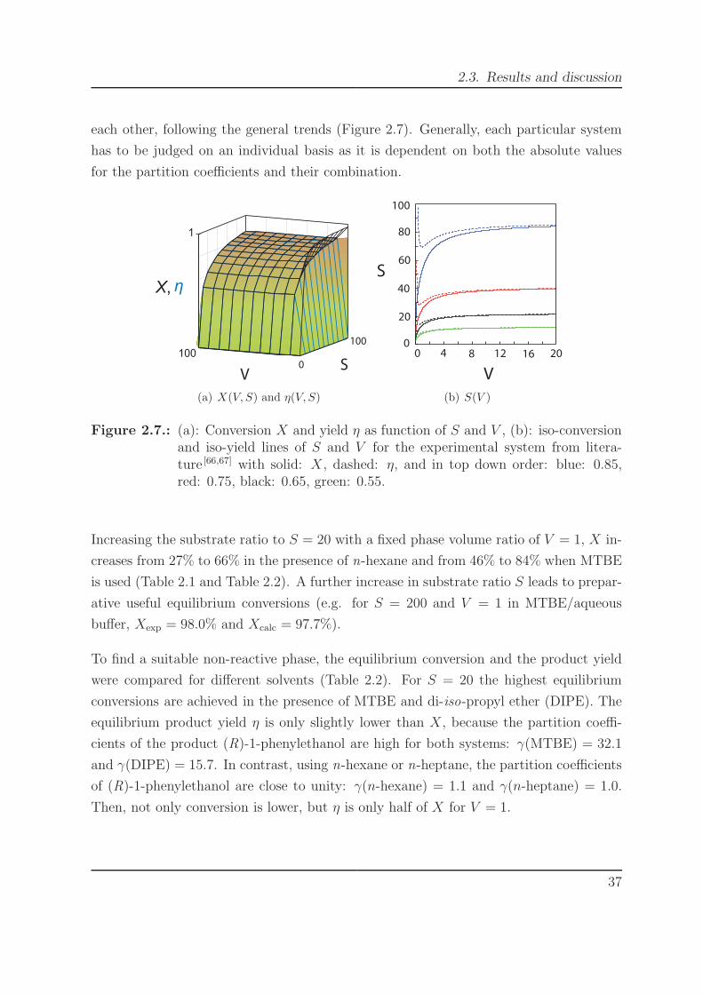
2.3. Results and discussion
each other, following the general trends (Figure 2.7). Generally, each particular system
has to be judged on an individual basis as it is dependent on both the absolute values
for the partition coefficients and their combination.
V
100
S
100
X, η
1
0
(a) X(V, S) and η(V, S)
0
20
40
60
80
0 12 16 20
S
V
84
100
(b) S(V )
Figure 2.7.: (a): Conversion X and yield η as function of S and V , (b): iso-conversionand iso-yield lines of S and V for the experimental system from litera-ture [66,67] with solid: X, dashed: η, and in top down order: blue: 0.85,red: 0.75, black: 0.65, green: 0.55.
Increasing the substrate ratio to S = 20 with a fixed phase volume ratio of V = 1, X in-
creases from 27% to 66% in the presence of n-hexane and from 46% to 84% when MTBE
is used (Table 2.1 and Table 2.2). A further increase in substrate ratio S leads to prepar-
ative useful equilibrium conversions (e.g. for S = 200 and V = 1 in MTBE/aqueous
buffer, Xexp = 98.0% and Xcalc = 97.7%).
To find a suitable non-reactive phase, the equilibrium conversion and the product yield
were compared for different solvents (Table 2.2). For S = 20 the highest equilibrium
conversions are achieved in the presence of MTBE and di-iso-propyl ether (DIPE). The
equilibrium product yield η is only slightly lower than X, because the partition coeffi-
cients of the product (R)-1-phenylethanol are high for both systems: γ(MTBE) = 32.1
and γ(DIPE) = 15.7. In contrast, using n-hexane or n-heptane, the partition coefficients
of (R)-1-phenylethanol are close to unity: γ(n-hexane) = 1.1 and γ(n-heptane) = 1.0.
Then, not only conversion is lower, but η is only half of X for V = 1.
37
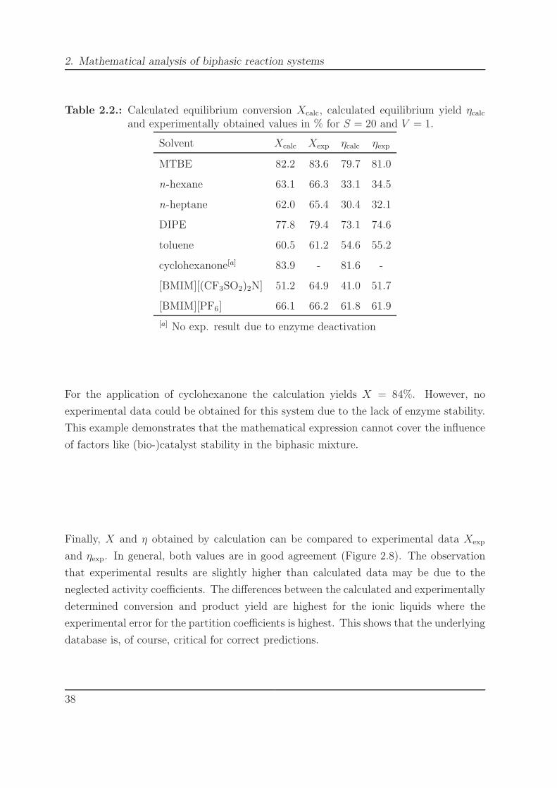
2. Mathematical analysis of biphasic reaction systems
Table 2.2.: Calculated equilibrium conversion Xcalc, calculated equilibrium yield ηcalc
and experimentally obtained values in % for S = 20 and V = 1.
Solvent Xcalc Xexp ηcalc ηexp
MTBE 82.2 83.6 79.7 81.0
n-hexane 63.1 66.3 33.1 34.5
n-heptane 62.0 65.4 30.4 32.1
DIPE 77.8 79.4 73.1 74.6
toluene 60.5 61.2 54.6 55.2
cyclohexanone[a] 83.9 - 81.6 -
[BMIM][(CF3SO2)2N] 51.2 64.9 41.0 51.7
[BMIM][PF6] 66.1 66.2 61.8 61.9
[a] No exp. result due to enzyme deactivation
For the application of cyclohexanone the calculation yields X = 84%. However, no
experimental data could be obtained for this system due to the lack of enzyme stability.
This example demonstrates that the mathematical expression cannot cover the influence
of factors like (bio-)catalyst stability in the biphasic mixture.
Finally, X and η obtained by calculation can be compared to experimental data Xexp
and ηexp. In general, both values are in good agreement (Figure 2.8). The observation
that experimental results are slightly higher than calculated data may be due to the
neglected activity coefficients. The differences between the calculated and experimentally
determined conversion and product yield are highest for the ionic liquids where the
experimental error for the partition coefficients is highest. This shows that the underlying
database is, of course, critical for correct predictions.
38
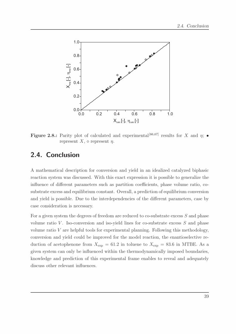
2.4. Conclusion
0.0 0.2 0.4 0.6 0.8 1.00.0
0.2
0.4
0.6
0.8
1.0
X [-], [-]calc calch
X[-
],[-
]e
xp
exp
h
Figure 2.8.: Parity plot of calculated and experimental [66,67] results for X and η; •
represent X, ⋄ represent η.
2.4. Conclusion
A mathematical description for conversion and yield in an idealized catalyzed biphasic
reaction system was discussed. With this exact expression it is possible to generalize the
influence of different parameters such as partition coefficients, phase volume ratio, co-
substrate excess and equilibrium constant. Overall, a prediction of equilibrium conversion
and yield is possible. Due to the interdependencies of the different parameters, case by
case consideration is necessary.
For a given system the degrees of freedom are reduced to co-substrate excess S and phase
volume ratio V . Iso-conversion and iso-yield lines for co-substrate excess S and phase
volume ratio V are helpful tools for experimental planning. Following this methodology,
conversion and yield could be improved for the model reaction, the enantioselective re-
duction of acetophenone from Xexp = 61.2 in toluene to Xexp = 83.6 in MTBE. As a
given system can only be influenced within the thermodynamically imposed boundaries,
knowledge and prediction of this experimental frame enables to reveal and adequately
discuss other relevant influences.
39

2. Mathematical analysis of biphasic reaction systems
40
3. Calculating partition coefficients
using COSMO-RS
3.1. Introduction
To pave the way to an ab inito solvent screening for biphasic systems, prediction of
solvent dependent parameters is a prerequisite. After the analysis of the thermodynamic
situation of the system in the previous chapter, investigation of the phase equilibria is the
target of this chapter. The performance of COSMO-RS for the prediction of equilibrium
partitioning of enzyme-catalyzed oxidoreductions in biphasic media will be tested. At
first, the quantitative performance for a specific reaction and solvent and then for a set
of substrates and solvents is evaluated. The results are used for a solvent screening of a
defined reaction based on equilibrium conversion as optimization target.
3.2. Materials and methods
3.2.1. Computational
The software GaussView (Version 3.09, Gaussian Inc., Wallingford, US) was used to
assemble all molecules. The DFT/COSMO (Conductor-like screening model [51]) calcula-
tions were performed using TURBOMOLE (Version 5.7.1, COSMOlogic, Leverkusen,
Germany) with the BP86 density functional and a TZVP basis set combination. [54]
41
3. Calculating partition coefficients using COSMO-RS
For the following statistical thermodynamics, the software COSMOtherm (Version C2.1-
0104/C2.1-0105, COSMOlogic, Leverkusen, Germany) was used based on the conductor-
like screening model for realistic solvation (COSMO-RS). [53,70] Partition coefficients at
infinite dilution are a direct result of COSMOtherm calculations:
P 21i =
exp(µ1i − µ2
i )
RT
υ1
υ2. (3.1)
In chemical engineering partition coefficients are usually reported in mole fractions, while
in chemistry the unit of choice is usually mol/l. Although a partition coefficient is di-
mensionless in both conventions, it differs by the ratio of the molar volumes of the two
solvents. [71] The ratio of the molar volumes was estimated from the COSMO volumes
since only ambient temperatures and pressures were considered here. The mutual sol-
ubility of the solvents was taken into account using an experimental data collection. [72]
These calculations at infinite dilution have been performed by the author of this thesis.
All quantum chemical calculations were carried out on the high performance computer
cluster of the Center for Computing and Communication, RWTH Aachen University,
Germany.
The equilibrium partitioning at finite concentrations, however, was determined iteratively
using the activity coefficients calculated by COSMOtherm. In contrast to the calculations
at infinite dilution, no experimental data on phase composition could be inserted into the
calculations. The iteration was carried out until activity coefficients were constant:
γ1i x
1 = γ2i x
2. (3.2)
The resulting molar fractions x2i and x1
i of both phases could then be used to calculate the
volumetric equilibrium concentrations. These calculations at finite concentrations were
performed by W. Eberhard, Biochemical Process Engineering, RWTH Aachen University,
Germany, as part of his PhD thesis.
The calculations of equilibrium conversion were performed both with COSMO-RS cal-
culated partition coefficients at infinite dilution and with experimentally determined
partition coefficients. These calculations were performed by the author of this thesis.
42
3.2. Materials and methods
3.2.2. Experimental
Experimental determination of partition coefficients at finite dilution was performed by
W. Eberhard, Biochemical Process Engineering, RWTH Aachen University, Germany,
as part of his PhD thesis. For the measurement of concentration dependent partition
coefficients at 25◦C (measurement range between 1.5mM and 350 mM), quantities of
water, solvent and substrate were filled into screw capped glass vials. The headspace
was minimized to reduce the loss of volatile material. The vials were repetitively shaken
and left for one week. Samples were taken from the organic phase and analyzed by GC.
For formic acid, the aqueous phase was sampled from an upside-down vial in order not
to penetrate the organic phase during sampling and the equilibrium concentration was
determined using HPLC. All measurements were carried out at least 7-fold.
Infinite dilution partition coefficients and equilibrium conversions were experimentally
determined by M. Eckstein as part of her PhD thesis [65] and by Julia Lembrecht (both
Technical Chemistry, University of Rostock, Germany) as part of her diploma thesis. All
infinite dilution partition coefficient measurements were carried out at least 7-fold.
For the determination of partition coefficients of acetophenone and 1-phenylethanol, sub-
strate solutions for each compound were prepared in the desired solvents. In screw-capped
vials the aqueous phase was covered with the same amount of organic phase. The sam-
ples were shaken (30◦C, 400 rpm). The mixtures were stored in a water bath (30◦C, 3
days). Samples were taken from each phase and analyzed by GC.
For the measurement of partition coefficients of acetone and 2-propanol the procedure
is different. Since the analytical method to quantify 2-propanol and acetone is based on
HPLC applying an aqueous eluent, samples could only be measured out of the aqueous
phase. Therefore, substrate solutions were prepared in water and buffer, respectively,
and the aqueous phase was covered with the desired organic solvents. To determine
partition coefficients of acetone and 2-propanol, samples were taken from the aqueous
phase before and after the addition of organic solvent and were measured by HPLC. The
partition coefficients P could then be calculated following the decline of concentration in
the aqueous phase.
For the measurement of equilibrium conversion and yield, an aqueous solution (2.5 mL)
43
3. Calculating partition coefficients using COSMO-RS
of LB-ADH, NADP+ (0.1 mmolL−1) and 2-propanol was covered with the organic sol-
vent containing acetophenone (20 to 80 mM). The mixture was shaken in a vertical
shaker (30◦C, 200 rpm). Samples were withdrawn from the non-reactive organic phase
and analyzed by GC. To get to values for conversion and yield, mass balances of ace-
tophenone and 1-phenylethanol were corrected by their partition coefficients. Complete
experimental details are described elsewhere. [66,67]
3.3. Results and discussion
3.3.1. Alcohol dehydrogenase catalyzed reductions
The biocatalytic asymmetric reduction of acetophenone to (R)-1-phenylethanol using
LB -ADH as biocatalyst (Figure 2.1 on page 35) is a typical example for a reaction where
a biphasic system is particularly advantageous. Interesting substrates typically exhibit
a low solubility in water, whereas the alcohol dehydrogenases are considerable more
effective in aqueous environment. Therefore, aqueous-organic [11,73,74] and aqueous–ionic
liquid systems [20,75] are in use. The addition of an immiscible solvent to the reaction
system will influence the overall reaction equilibrium by partitioning of all substrates and
products between the non-reactive organic and the reactive aqueous phase (Figure 2.1
on page 26).
The design and optimization of the reaction system requires the knowledge of the parti-
tioning of all substrates and products between both phases. For a biocatalytic esterifica-
tion in aqueous-organic two-phase systems, it was previously found that non-ideal parti-
tioning occurs. [76] Therefore, calculations and measurements of concentration-dependent
partition coefficients were performed.
3.3.2. Calculation of concentration-dependent partition coefficients
The first system investigated was the reduction of acetophenone and a functionalized
derivative (2-chloroacetophenone) to the corresponding alcohols in the biphasic reaction
44
3.3. Results and discussion
medium n-hexane/water. The formate dehydrogenase (FDH) coupled cofactor regenera-
tion with formic acid as co-substrate yielded gaseous carbon dioxide as co-product, thus
driving the reaction equilibrium to the desired product. The predicted concentration
dependent phase equilibria, those at infinite dilution and experimental data points for
the distribution of acetophenone, 1-phenylethanol, 2-chloroacetophenone and formic acid
in n-hexane/water are given in Figure 3.1.
As indicated by the experimental values, the solutes show a non-linear concentration-
dependent distribution between the organic and the aqueous phase. For acetophenone
(Figure 3.1(a)), COSMO-RS predictions for finite concentrations are both qualitatively
and quantitatively in good agreement. The solubility limit in the aqueous buffer phase
is reached at around 15 mM. For the corresponding reaction product, 1-phenylethanol
(Figure 3.1(b)), however, larger deviations between the prediction and the experimental
data occur. The same, even stronger effect can be observed for the chloro-substituted ace-
tophenone (Figure 3.1(c)). In both cases, a more hydrophobic character of the substances
is predicted than determined experimentally. A similar overestimation of octanol/water
partition coefficients for alcohols and chloro-substituted compounds has been observed
previously. [77] Even the deviation of up to factor 10 lies within the previously published
prediction accuracy. For formic acid (Figure 3.1(d)), however, the predicted and experi-
mental values deviate within two orders of magnitude. In the same plot the prediction of
the formic acid concentration is not distinguishable from the ordinate. Only in the insert
in Figure 3.1(d) can it be seen that the aqueous formic acid concentration differs from
infinity. The deviations here can be attributed to the formation of dimers of the acid
in the organic phase. [76,78] The mere statistical approach of COSMO-RS is not capable
of representing this associating behavior of a chemical compound. The consideration of
conformers in case of alcohols and of dimers in case of carboxylic acids during the quan-
tum mechanical calculation of the molecular surface will most probably lead to better
quantitative results.
One source of error in the prediction of partition coefficients is the mutual solubility
of the solvents. This cannot be taken into account in the calculation of finite parti-
tion coefficients using COSMO-RS leading to a significant error. Opposite to that, in
the COSMO-RS calculation of infinite dilution partition coefficients the mutual solu-
bility can be considered. This is possible either via direct calculation of liquid-liquid
45
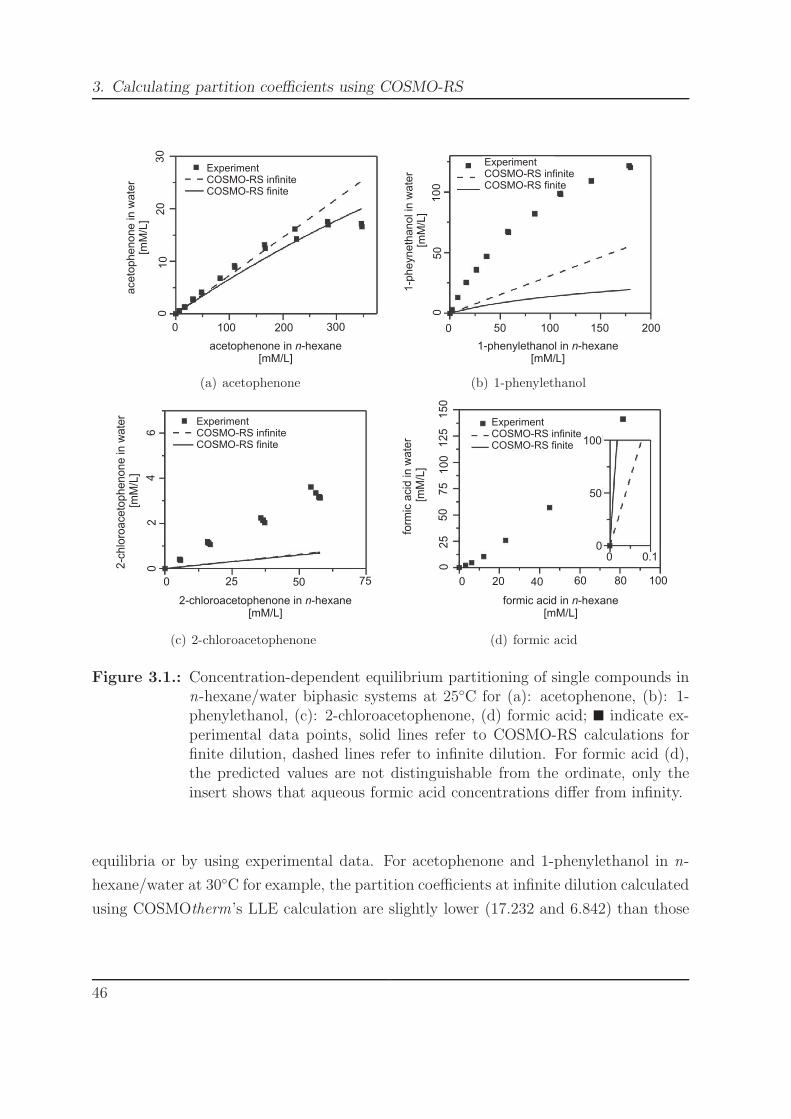
3. Calculating partition coefficients using COSMO-RS
ExperimentCOSMO-RS infiniteCOSMO-RS finite
acetophenone in -hexane[mM/L]
n
ace
top
he
no
ne
in
wa
ter
[mM
/L]
0 100 200 300
01
02
03
0
(a) acetophenone
ExperimentCOSMO-RS infiniteCOSMO-RS finite
1-phenylethanol in -hexane[mM/L]
n
1-p
he
yn
eth
an
ol in
wa
ter
[mM
/L]
0 50 100 150
05
01
00
200
(b) 1-phenylethanol
ExperimentCOSMO-RS infiniteCOSMO-RS finite
2-chloroacetophenone in -hexane[mM/L]
n
2-c
hlo
roa
ce
top
he
no
ne
in w
ate
r[m
M/L
]
0 25 50 75
02
46
(c) 2-chloroacetophenone
ExperimentCOSMO-RS infiniteCOSMO-RS finite
formic acid in -hexane[mM/L]
n
form
ic a
cid
in w
ate
r[m
M/L
]
0 20 40 60
02
55
07
5
80 100
10
01
25
15
0
0.100
50
100
(d) formic acid
Figure 3.1.: Concentration-dependent equilibrium partitioning of single compounds inn-hexane/water biphasic systems at 25◦C for (a): acetophenone, (b): 1-phenylethanol, (c): 2-chloroacetophenone, (d) formic acid; � indicate ex-perimental data points, solid lines refer to COSMO-RS calculations forfinite dilution, dashed lines refer to infinite dilution. For formic acid (d),the predicted values are not distinguishable from the ordinate, only theinsert shows that aqueous formic acid concentrations differ from infinity.
equilibria or by using experimental data. For acetophenone and 1-phenylethanol in n-
hexane/water at 30◦C for example, the partition coefficients at infinite dilution calculated
using COSMOtherm’s LLE calculation are slightly lower (17.232 and 6.842) than those
46

3.3. Results and discussion
calculated using the experimental LLE (19.231 and 8.621).
Although the prediction of partitioning at finite dilution better represents the qualita-
tive behavior of the solute partitioning between the aqueous and n-hexane phase, the
prediction of partitioning at infinite dilution is equal (for 2-chloroacetophenone) or supe-
rior (in all other cases) in quantitative terms. Therefore, only infinite dilution partition
coefficients were predicted for further studies. A similar approach was chosen previously
for the prediction of partitioning using UNIFAC. [79]
3.3.3. Calculation of infinite dilution partition coefficients
A set of experimentally determined partition coefficients was compared to the COSMO-
RS predicted partition coefficients at infinite dilution. In order to eliminate the system-
atic error of formic acid, the chosen solutes now cover substances used in the reduction
of aliphatic ketones and acetophenone derivatives with a substrate-coupled cofactor re-
generation using isopropanol as co-substrate in several biphasic solvent combinations
(n-hexane, n-heptane, MTBE, toluene, cyclohexanone, each coupled with water). In
the experimentally covered concentration range from 10 mM to 100 mM, the partition
coefficients did not vary, but remained constant. Therefore, they are considered a good
approximation to infinite dilution. The numerical values for the experimental data can
be found in the original literature. [65–67]
Figure 3.2 shows a logarithmic parity plot of the predicted infinite dilution partition
coefficients over three sets of experimentally determined data. The first data set covers
substrates and products of the acetophenone reduction using 2-propanol as co-substrate
in several solvent systems. [66] The second set covers linear ketones and some acetophe-
none derivatives and their corresponding alcohols in MTBE/water biphasic systems. [65]
The third data set covers the same compounds as the second, but in a n-hexane/water
biphasic system. [67] A certain bias towards overestimation of the partition coefficients
towards hydrophobicity as mentioned above can be observed. The lower 95% boundary
corresponds to factor 2.5 units (0.4 log(P∞)) deviation, and the upper 95% boundary to
factor 8 (0.9 log(P∞) units). A calculation of the root mean square (rms) deviation re-
sults in 0.25 log(P∞) units. Even the COSMO-RS parameterization data set has a higher
47

3. Calculating partition coefficients using COSMO-RS
Figure 3.2.: Comparison of experimental and COSMO-RS predicted infinite dilutionpartition coefficients P∞ at 30◦C for single selected substrates and prod-ucts in organic/aqueous biphasic reaction systems; • indicate the datapoints corresponding to reference [66], N those of [65], and H those of [67], thethick solid line indicates parity; the thin dashed lines enclose 95% of thedata points; please note the logarithmic scaling.
rms deviation of 0.34 log(P∞) units. [80] The prediction of the octanol-water partition co-
efficient log Pow for more than 60 compounds resulted in a slightly inferior deviation of
0.43 log Pow units (rms). [77] In comparison to the prediction accuracy (0.64-0.83 log Pow
units rms) of two UNIFAC versions, [77] the predictive power of COSMO-RS becomes
apparent.
48

3.3. Results and discussion
3.3.4. Solvent screening: partition coefficients
The screening of solvent combinations for one specific oxidoreduction reaction is now car-
ried out by again predicting infinite dilution partition coefficients using COSMO-RS. To
reduce the prediction error, experimental data was used for the mutual solubility of the
solvents. [72] The investigated reaction is the LB -ADH catalyzed reduction of acetophe-
none to (R)-1-phenylethanol using the 2-propanol coupled regeneration with acetone as
co-product (Figure 2.1 on page 35). An overview about partition coefficient prediction
for all solutes across several solvents is given in Figure 3.3. The solvents cover a repre-
sentative range of organic solvents which are often used for enzyme catalyzed biphasic
reaction systems.
Figure 3.3 indicates that the prediction of partition coefficients of ketones in several
solvent combinations is more successful than that of the corresponding alcohols. The
predicted partition coefficients at infinite dilution of acetophenone (Figure 3.3(a)) and
acetone (Figure 3.3(d)) have a relative error of less than 30% with respect to the mea-
sured partition coefficients. Nearly quantitative prediction is obtained for acetophenone
in linear alkane/water solvent combination. A bias to underestimate the infinite dilution
partition coefficients of ketones can be observed for all solvent combinations. In contrast
to the ketones, the infinite dilution partition coefficients of (R)-1-phenylethanol are over-
estimated for all solvent combinations (Figure 3.3(b)). Only the partitioning of the very
small 2-propanol molecule is in good agreement in toluene and even underestimated in
linear alkanes (Figure 3.3(c)). The prediction accuracy for the studied reaction system
is within one order of magnitude on a linear scale. Looking at the sequence of partition
coefficients for one solute across several solvent combinations, COSMO-RS is capable of
predicting the correct trends. Nevertheless, care should be taken for protic solvents, since
their ability to form hydrogen bonds is to date not sufficiently covered by COSMO-RS.
3.3.5. Solvent screening: equilibrium conversion
Having identified correct trends for infinite dilution partition coefficients for all reactants,
the solvent combinations may now be compared with respect to the target function of
maximum conversion (equation 2.13 on page 28). The reaction equilibrium constant
49

3. Calculating partition coefficients using COSMO-RS
0 20 40 60 80 100 120 1400
20
40
60
80
100
120
140
Experimental partition coefficient
Calc
uate
d p
art
itio
n c
oeffic
ient
(a) acetophenone
0 20 40 60 80 100 120 140 160 180 2000
20
40
60
80
100
120
140
160
180
200
Experimental partition coefficient
Calc
uate
d p
art
itio
n c
oeffic
ient
(b) (R)-1-phenylethanol
0.0 0.5 1.0 1.5 2.0 2.5 3.0 3.5 4.0 4.50.0
0.5
1.0
1.5
2.0
2.5
3.0
3.5
4.0
4.5
Experimental partition coefficient
Calc
uate
d p
art
itio
n c
oeffic
ient
(c) 2-propanol
Experimental partition coefficient
0.0 0.2 0.4 0.6 0.8 1.0 1.2 1.4 1.60.0
0.2
0.4
0.6
0.8
1.0
1.2
1.4
1.6
Calc
uate
d p
art
itio
n c
oeffic
ient
(d) acetone
Figure 3.3.: Experimental and COSMO-RS predicted infinite dilution partition coef-ficients of single compounds at 30◦C of (a): acetophenone, (b): (R)-1-phenylethanol, (c): 2-propanol, and (d): acetone in various organic sol-vent/water systems with •: n-hexane/water, H: n-heptane/water, �:MTBE/water, N: cyclohexanone/water, �: toluene/water. Note the dif-ference in scaling.
K (=0.426 at 30◦C) is intrinsically defined by the aqueous reaction environment. The
substrate ratio S = 20 and the phase volume ratio V = 1 are kept constant across
all solvent combinations. Thus, the maximum conversion may be calculated using the
predicted partition coefficients at infinite dilution Xcalc,ab initio, and compared with both
50

3.3. Results and discussion
the calculated conversion using the experimentally determined partition coefficients Xcalc
and the experimental equilibrium conversion Xexp (Figure 3.4).
100
80
60
40
20
0
Convers
ion
[%]
X
n-h
exan
e/H
O2
n-h
epta
ne/H
O2
MTBE/H
O2
tolu
ene/
HO2
cycloh
exan
one/
HO2
Xexp
Xcalc
Xcalc,ab-initio
Figure 3.4.: Equilibrium conversion of the reduction of acetophenone to (R)-1-phenylethanol by oxidizing 2-propanol in various organic solvent/watersystems with K = 0.426; S = 20; V = 1; black bars indicate experi-mental values Xexp,
[66,67] dark grey bars represent the calculated conver-sion based on experimentally determined partition coefficients Xcalc, lightgrey bars show the calculated conversion based on the COSMO-RS pre-dicted partition coefficients at infinite dilution Xcalc,ab initio; for the cyclo-hexanone/water system no experimental data could be obtained.
The screening target theoretical conversion as calculated based on predicted infinite di-
lution partition coefficients Xcalc,ab initio shows a systematic deviation of roughly +20%
from the corresponding experimental data (Figure 3.4). The analogously calculated con-
version using experimentally determined partition coefficients Xcalc, however, is in good
agreement with the directly measured Xexp. Therefore, it appears that the error contri-
bution of the underlying ideality assumption in equation 2.13 on page 28 does not have
a major effect. Although this assumption is in contrast to the non-ideal partitioning of
51

3. Calculating partition coefficients using COSMO-RS
the investigated reaction systems (Figure 3.1), the influence on the maximum conver-
sion is negligible in comparison to the deviation in the predicted partition coefficients.
The error contribution may be explained by analyzing equation 2.12 on page 28. The
overall reaction equilibrium constant is corrected by an expression containing the phase
volume ratio and the partition coefficients. The overestimation of (R)-1-phenylethanol
partition coefficients contributes strongest to the factor m, thus resulting in an overesti-
mated overall reaction equilibrium constant mK. This again leads to a higher calculated
equilibrium conversion.
Even if the absolute values for predicted conversions deviate in analogy to the prediction
of individual partition coefficients, the overall trends are again represented well. One
reason for this is that errors may cancel out in a reaction situation where functional
groups such as ketones and alcohols are retained during the reaction. The highest ex-
perimentally determined conversion was successfully identified by the highest predicted
conversion as shown in Table 3.1. The table also underlines that the ranking order of
Xexp and Xcalc,ab initio for the systems n-heptane/water and toluene/water differ from
each other. However, the difference lies within the first decimal place representing the
limit of the predictions.
Table 3.1.: Ranking order of equilibrium conversion of the reduction of acetophenoneto 1-phenylethanol by oxidizing 2-propanol in various organic solvent/watersystems; bold red figures indicate a difference in the ranking order comparedto Xexp.
Solvent combination Xexp Xcalc Xcalc,ab initio
MTBE/water 83.5 82.8 93.9
n-hexane/water 65.8 63.2 83.9
n-heptane/water 65.3 62.0 83.0
toluene/water 61.2 60.5 83.2
cyclohexanone/water 0.0 83.9 92.3
Looking at the solvent combination cyclohexanone/water in Table 3.1, however, the
second highest conversion was predicted both using predicted and experimentally deter-
52
3.4. Conclusion
mined partition coefficients, but was not reached experimentally since the enzyme did
not retain sufficient activity in this solvent combination. This is an often observed effect
for solvents of moderate hydrophobicity, [81] also for oxidoreduction reactions. [11] It brings
the alternative solvent screening targets back into mind: Enzyme activity, selectivity, and
stability. Thus, the thermodynamic screening may indeed be performed in silico, but an
experimental validation of the top solvent candidates is mandatory. Even with a final
confirmation run, the in silico screening approach will still save considerable laboratory
effort because it allows to identify targets for further development and optimization.
3.4. Conclusion
For the design of biocatalytic biphasic reaction systems, the knowledge of partition equi-
libria for all reactants in suitable solvent systems is helpful for process modeling as
well as for the targeted solvent screening. The quantum mechanical and statistical
thermodynamics-based tool COSMO-RS was evaluated with respect to this quantita-
tive task, i.e. prediction of finite and infinite dilution partition coefficients for modeling
purpose and the qualitative task of solvent screening for maximum conversion.
Although non-ideal equilibrium partitioning was well predicted, the infinite dilution par-
tition coefficients calculations still lead to smaller overall deviations from the experi-
mental values than finite dilution partition coefficient calculations. Consequently, the
more sophisticated approaches to overall reaction equilibrium calculations taking the
changing reactant partitioning during the reaction into account (non-ideal equilibrium
partitioning) seem exaggerated at the current stage. For the selected components the
experimental data were systematically better represented than by other tools, but an
improvement of the quantitative performance would still be highly desirable for a more
in-depth process design.
For qualitative tasks like solvent screening, however, the quality of prediction seems suf-
ficient since the ranking order of solvents for a chemical compound regarding infinite
dilution partition coefficients was predicted correctly. Based on these data, the theo-
retical conversion could be calculated, resulting in the selection of suitable solvents for
the asymmetric biphasic reduction of acetophenone to (R)-1-phenylethanol. A ranking
53

3. Calculating partition coefficients using COSMO-RS
of solvents in view of theoretical conversion was achieved, systematic deviations in pre-
dicted partition coefficients for individual compounds neutralize in the reaction context.
The experimental validation of this choice will remain necessary with respect to solvent
tolerance of the catalyst and solvation effects that influence the catalytic performance,
such as activity, specificity, and selectivity.
54
4. Calculating equilibrium constants
4.1. Introduction
The last step to the ab initio solvent screening is an in silico prediction of the equi-
librium constant of a reaction. Therefore, the investigation of solvation processes is a
prerequisite. In order to know how one can influence processes in solution, the standard
Gibbs energies of reaction in solution are of great interest. Experimental values as well
as electrochemical potentials are found only sparsely in literature. The reason for this
lack is that either the measurements are considered routine, although advanced tech-
niques and laborious protocols are needed for reliable data, or the direct measurement
is impossible. [67] In the context of this thesis, the knowledge of standard Gibbs energies
of reaction in solution ∆Gsolutionr paves the way to a straightforward and cost-effective
computational solvent screening for equilibrium conversion and yield.
4.2. Materials and methods
4.2.1. Computational
The molecules were assembled using the software GaussView (Version 3.09, Gaussian
Inc., Wallingford, US). [82] The geometry optimizations and the frequency calculations
for each molecule were carried out using the B3LYP/TZVP method using the software
Gaussian 03. [83]
55

4. Calculating equilibrium constants
On top of that the calculations led to a term accounting for thermal correction to the
Gibbs free energies of reaction in the gas phase. This term was added to the gas phase
energies. The latter were calculated via single point calculations using the software
Gaussian and the different quantum chemical methods B3LYP/TZVP, MP2/TZVP and
CCSD(T)/cc-pVTZ. The standard state for the Gaussian calculations is a pressure of
1013 hPa and a temperature of 298.15 K.
The calculations of the gas phase energies for COSMO-RS and the energies in a conductor
were performed using TURBOMOLE (Version 5.8, COSMOlogic GmbH, Leverkusen,
Germany) with RI-BP86 functional and TZVP basis set. [84–86]
The energies of solvation were calculated using the software COSMOtherm (Version C2.1,
Release 01.05, COSMOlogic GmbH, Leverkusen, Germany). [80,87] The different basis sets
used for the calculations in the gas and the liquid phase were chosen according to the
recommendation of COSMOlogic, the distributor of COSMOtherm. Standard state for
the calculation of Gibbs free energy of solvation ∆Gsolv is the fluid hypothetical ideally
diluted at 1 M concentration. All quantum chemical calculations were performed by the
author of this thesis and carried out on the high performance computer cluster of the
Center for Computing and Communication, RWTH Aachen University, Germany.
4.2.2. Experimental
The experimental data for ∆Gideal gasr were taken from literature, [88] the experimental
data for ∆Gsolutionr were taken from literature as well. [89]
4.3. Results and discussion
The overall aim was to establish an easy-to-handle procedure for the calculation of stan-
dard Gibbs energies of reaction in solution ∆Gsolutionr . Based on a Hessian cycle in
Figure 4.1, ∆Gsolutionr can be calculated by summing up the values for the Gibbs free
56
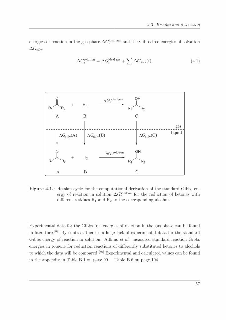
4.3. Results and discussion
energies of reaction in the gas phase ∆Gideal gasr and the Gibbs free energies of solvation
∆Gsolv:
∆Gsolutionr = ∆Gideal gas
r +∑
∆Gsolv(i). (4.1)
Figure 4.1.: Hessian cycle for the computational derivation of the standard Gibbs en-ergy of reaction in solution ∆Gsolution
r for the reduction of ketones withdifferent residues R1 and R2 to the corresponding alcohols.
Experimental data for the Gibbs free energies of reaction in the gas phase can be found
in literature. [88] By contrast there is a huge lack of experimental data for the standard
Gibbs energy of reaction in solution. Adkins et al. measured standard reaction Gibbs
energies in toluene for reduction reactions of differently substituted ketones to alcohols
to which the data will be compared. [89] Experimental and calculated values can be found
in the appendix in Table B.1 on page 99 − Table B.6 on page 104.
57

4. Calculating equilibrium constants
4.3.1. Gibbs free energy of reaction in the gas phase
When performing a quantum chemical geometry optimization, the equilibrium geometry
of the studied molecule and its energy are obtained. This is the energy of the molecule in
vacuum, at 0 K and without zero point energies (ZPE) of the internal vibration modes
of the molecule. To take the ZPE and finite temperatures into account, all internal
modes are assumed to be harmonic oscillators. The force constants of these oscillators
have to be computed, which are the 2nd derivatives of the energy with respect to the
internal coordinates. Then the ZPEs of these modes are obtained and translational,
rotational (based on the geometry of the molecule) and vibrational contributions to
internal energy, enthalpy and entropy need to be computed by statistical mechanics. [28]
These contributions are necessary to proceed from the energy, which is a result of the
Schrodinger equation, to the ∆Gideal gasr at a finite temperature.
From this data, the standard Gibbs energy of reaction in the gas phase can be computed
and compared to experimental data. It is important to note that the force constants are
2nd derivatives and therefore computationally much more demanding than mere ener-
gies. Fortunately, the corrections are relatively small compared to the quantum chemical
energies. Therefore, the most efficient approach is to choose a simpler method for the
thermodynamic corrections and a more sophisticated method for the quantum chemical
energy. Since the geometry is usually less sensitive to inaccuracies of the method than
the energy, but at the same time computationally more demanding, the geometry is often
calculated by a simpler method as well.
For the calculation of ∆Gideal gasr , energies in the gas phase and a term accounting for
thermal correction were summed up:
∆Gideal gasr = Egas phase + Gthermal correction. (4.2)
The method used for the calculation of the latter is DFT. Three different quantum
chemical methods were compared for the calculation of the energies: DFT, MP2 and
CCSD(T). Here, the accuracy in the calculations rises with DFT < MP2 < CCSD(T)
(Figure 4.2 and in the appendix Tables B.1, B.2, B.3). For ∆Gideal gasr , the magnitude of
58
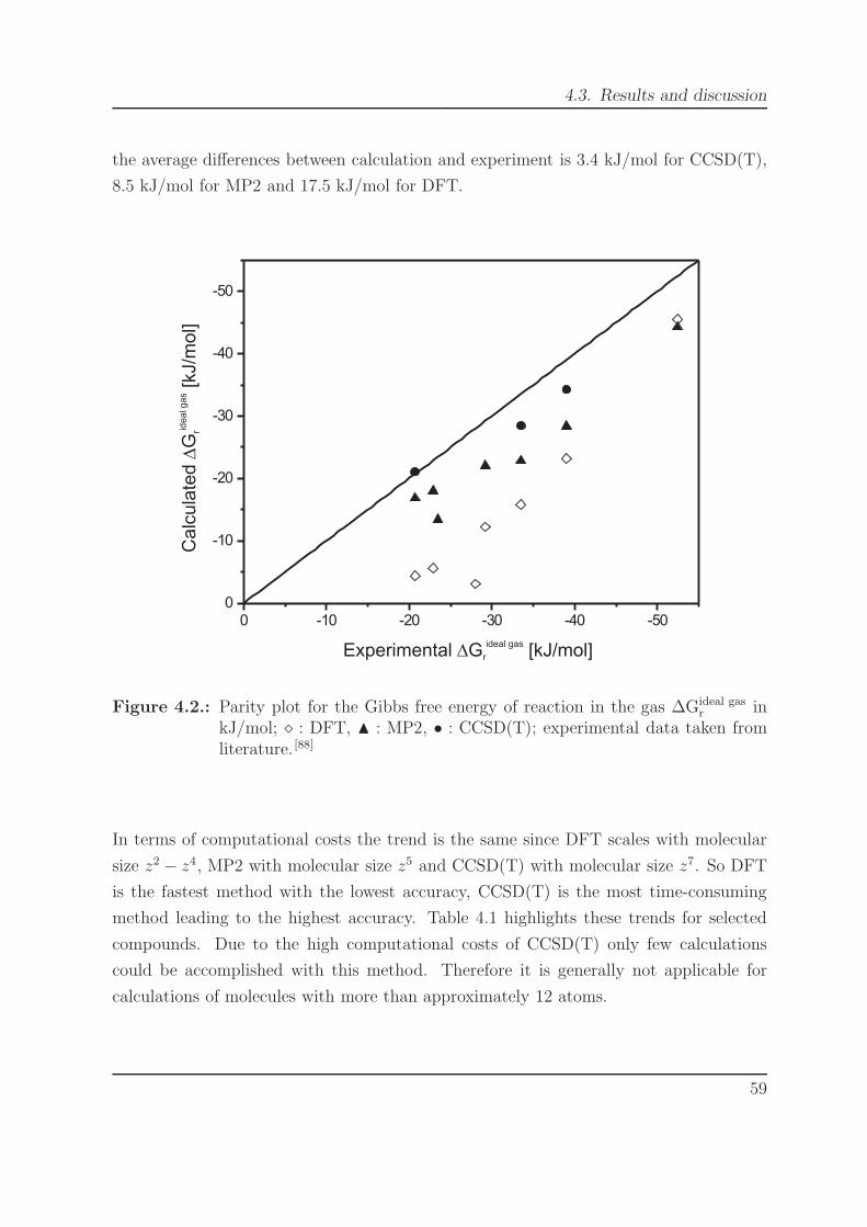
4.3. Results and discussion
the average differences between calculation and experiment is 3.4 kJ/mol for CCSD(T),
8.5 kJ/mol for MP2 and 17.5 kJ/mol for DFT.
0 -10 -20 -30 -40 -500
-10
-20
-30
-40
-50
Experimental G [kJ/mol]D r
ideal gas
Ca
lcu
late
dG
[kJ/m
ol]
Drid
ea
l g
as
Figure 4.2.: Parity plot for the Gibbs free energy of reaction in the gas ∆Gideal gasr in
kJ/mol; ⋄ : DFT, N : MP2, • : CCSD(T); experimental data taken fromliterature. [88]
In terms of computational costs the trend is the same since DFT scales with molecular
size z2 − z4, MP2 with molecular size z5 and CCSD(T) with molecular size z7. So DFT
is the fastest method with the lowest accuracy, CCSD(T) is the most time-consuming
method leading to the highest accuracy. Table 4.1 highlights these trends for selected
compounds. Due to the high computational costs of CCSD(T) only few calculations
could be accomplished with this method. Therefore it is generally not applicable for
calculations of molecules with more than approximately 12 atoms.
59

4. Calculating equilibrium constants
Table 4.1.: Comparison of job CPU time in s for the calculation of Gibbs free energies ofreaction in the gas phase ∆Gideal gas
r ; CPU time for geometry optimizationsat B3LYP/TZVP and single point energy calculations at B3LYP/TZVP,MP2/TZVP or CCSD(T)/cc-pVTZ summed up.
molecule calculation time for ∆Gideal gasr in s
B3LYP/TZVP MP2/TZVP CCSD(T)/cc-pVTZ
C2H4O (acetaldehyde) 120 180 21000
C3H6O (acetone) 480 660 152880
C4H8O (isobutanal) 1140 1620 323460
C5H10O (3-pentanone) 9120 10080 857220
4.3.2. Gibbs free energy of solvation
The Gibbs free energies of solvation ∆Gsolv can be calculated from Henry coefficients. For
the calculation of Henry coefficients, COSMO-RS was used. [80,87] Table 4.2 highlights the
speed of this kind of calculations. The calculated values for ∆Gsolv cannot be compared
to experimental values because no literature data is available for the specific reduction
reactions in toluene considered here.
Table 4.2.: Comparison of job CPU time in s for the calculation of Gibbs free ener-gies of solvation ∆Gsolv; geometry optimizations and single point energycalculations at BP86/TZVP.
molecule calculation time for ∆Gsolv in s
BP86/TZVP
C2H4O (acetaldehyde) 8
C3H6O (acetone) 16
C4H8O (isobutanal) 16
C5H10O (3-pentanone) 40
60

4.3. Results and discussion
4.3.3. Standard Gibbs energy of reaction in solution
Following the Hessian cycle depicted in Figure 4.1, the calculation of ∆Gsolutionr is possible
by adding up the values for the Gibbs free energies of reaction in the gas phase ∆Gideal gasr
and the Gibbs free energies of solvation ∆Gsolv according to equation (4.1). The results
are shown in Figure 4.3 and in Tables B.4, B.5, B.6 in the appendix. Surprisingly,
the quantum chemically most laborious method, CCSD(T), as well as the second most
laborious method, MP2, leads to similar results in terms of accuracy: For the standard
Gibbs energy of reaction in solution the magnitude of the difference between calculation
and experiment is 6.5 kJ/mol for CCSD(T), 6.1 kJ/mol for MP2 and 13.2 kJ/mol for
DFT. The good result for MP2 might be due to fortunate error cancelation effects caused
by the combination of COSMOtherm and MP2. DFT leads to less accurate results but
at the lowest computational costs.
0 -10 -20 -30 -40 -50 -60 -700
-10
-20
-30
-40
-50
-60
-70
Experimental G [kJ/mol]D r
solution
Ca
lcu
late
dG
[kJ/m
ol]
Drs
olu
tio
n
Figure 4.3.: Parity plot for the standard Gibbs energy of reaction in solution ∆Gsolutionr
in kJ/mol; ⋄ : DFT, N : MP2, • : CCSD(T); experimental data taken fromliterature. [89]
61
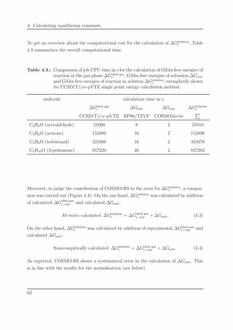
4. Calculating equilibrium constants
To get an overview about the computational cost for the calculation of ∆Gsolutionr , Table
4.3 summarizes the overall computational time.
Table 4.3.: Comparison of job CPU time in s for the calculation of Gibbs free energies ofreaction in the gas phase ∆Gideal gas
r , Gibbs free energies of solvation ∆Gsolv
and Gibbs free energies of reaction in solution ∆Gsolutionr ; exemplarily shown
for CCSD(T)/cc-pVTZ single point energy calculation method.
molecule calculation time in s
∆Gideal gasr ∆Gsolv ∆Gsolv ∆Gsolution
r
CCSD(T)/cc-pVTZ BP86/TZVP COSMOtherm∑
C2H4O (acetaldehyde) 21000 8 2 21010
C3H6O (acetone) 152880 16 2 152898
C4H8O (isobutanal) 323460 16 2 323478
C5H10O (3-pentanone) 857220 40 2 857262
Moreover, to judge the contribution of COSMO-RS to the error for ∆Gsolutionr , a compar-
ison was carried out (Figure 4.4): On the one hand, ∆Gsolutionr was calculated by addition
of calculated ∆Gideal gasr, calc and calculated ∆Gsolv:
Ab-initio calculated ∆Gsolutionr = ∆Gideal gas
r, calc + ∆Gsolv. (4.3)
On the other hand, ∆Gsolutionr was calculated by addition of experimental ∆Gideal gas
r, exp and
calculated ∆Gsolv:
Semi-empirically calculated ∆Gsolutionr = ∆Gideal gas
r, exp + ∆Gsolv. (4.4)
As expected, COSMO-RS shows a systematical error in the calculation of ∆Gsolv. This
is in line with the results for the normalization (see below).
62

4.3. Results and discussion
0 -10 -20 -30 -40 -50 -60 -700
-10
-20
-30
-40
-50
-60
-70
Semi-empirically calculated G [kJ/mol]D r
solution
Ab
-in
itio
ca
lcu
late
dG
[kJ/m
ol]
Drs
olu
tio
n
Figure 4.4.: Parity plot for the standard Gibbs energy of reaction in solution solu-tion ∆Gsolution
r in kJ/mol; semi-empirically calculated ∆Gsolutionr obtained
by addition of experimental ∆Gideal gasr,exp
[88] and calculated ∆Gsolv (equa-tion (4.3)), ab initio calculated ∆Gsolution
r obtained by addition of calcu-lated ∆Gideal gas
r, calc and calculated ∆Gsolv (equation (4.4)).
4.3.4. Experimental validation
The model reaction is the asymmetric substrate-coupled biocatalytic reduction of ace-
tophenone to (R)-phenylethanol (Figure 2.1 on page 35) in a biphasic reaction system
with one reactive phase. The solvent used as reactive phase is water. Possible solvent
candidates assessed are: n-hexane, n-heptane, MTBE, DIPE, toluene as well as the ionic
liquids [BMIM][BTA] and [BMIM][PF6].[65,66]
Before the actual screening can be started a precise definition of the target is impor-
tant, here, the maximization of equilibrium conversion and yield. The calculation and
prediction of equilibrium conversion and yield in biphasic reaction mixtures with only
63
4. Calculating equilibrium constants
one reactive phase is possible using the mathematical derivation introduced in Chapter
2 as a basis. For an ab initio solvent screening the calculation of partition coefficients of
all reactants is necessary as well as the calculation of equilibrium constant in the reac-
tive water phase. The partition coefficients were calculated using COSMOtherm, [90] the
equilibrium constant according to the method presented within this chapter.
Experimentally, the equilibrium constant was determined to be 2.15 kJ/mol, the cal-
culation yields 0.43 kJ/mol. There is a huge deviation in the absolute value, but the
positive sign for the equilibrium constant could be calculated correctly. Figure 4.5 shows
the results for experimental and ab initio predicted conversion X and yield η for the
biocatalytic reduction of acetophenone to (R)-phenylethanol for the different solvents
mentioned above. The solvent MTBE is the best solvent for the second phase in terms
of conversion and yield, predicted and experimentally verified. [66,67] Hence, a reasonable
ranking of the solvents is possible and the general trends predicted are correct.
Nevertheless, the absolute values for predicted conversion and yield might differ substan-
tially from the experimental values. Thus, in order to achieve quantitative values, the
predicted values for conversion and yield were normalized to one experimental result, here
to the median of experimental conversion and yield (Figure 4.5). This procedure gives
satisfactory values within the experimental error using a minimum of one experimental
point for conversion and yield, respectively.
4.4. Conclusion
A straightforward computational way for the prediction of standard Gibbs energies of
reaction in solution ∆Gsolutionr was presented using quantum mechanics as well as the
statistical thermodynamics as implemented in COSMO-RS. After quantum chemical ge-
ometry optimizations, the Gibbs free energies in the gas phase ∆Gideal gasr including the
zero point energies were determined. The Gibbs free energies of solvation ∆Gsolv were
calculated using the COSMOtherm program.
From these values the standard Gibbs energies of reaction in solution ∆Gsolutionr could
be calculated according to a Hessian cycle by adding up ∆Gideal gasr and ∆Gsolv. For
64
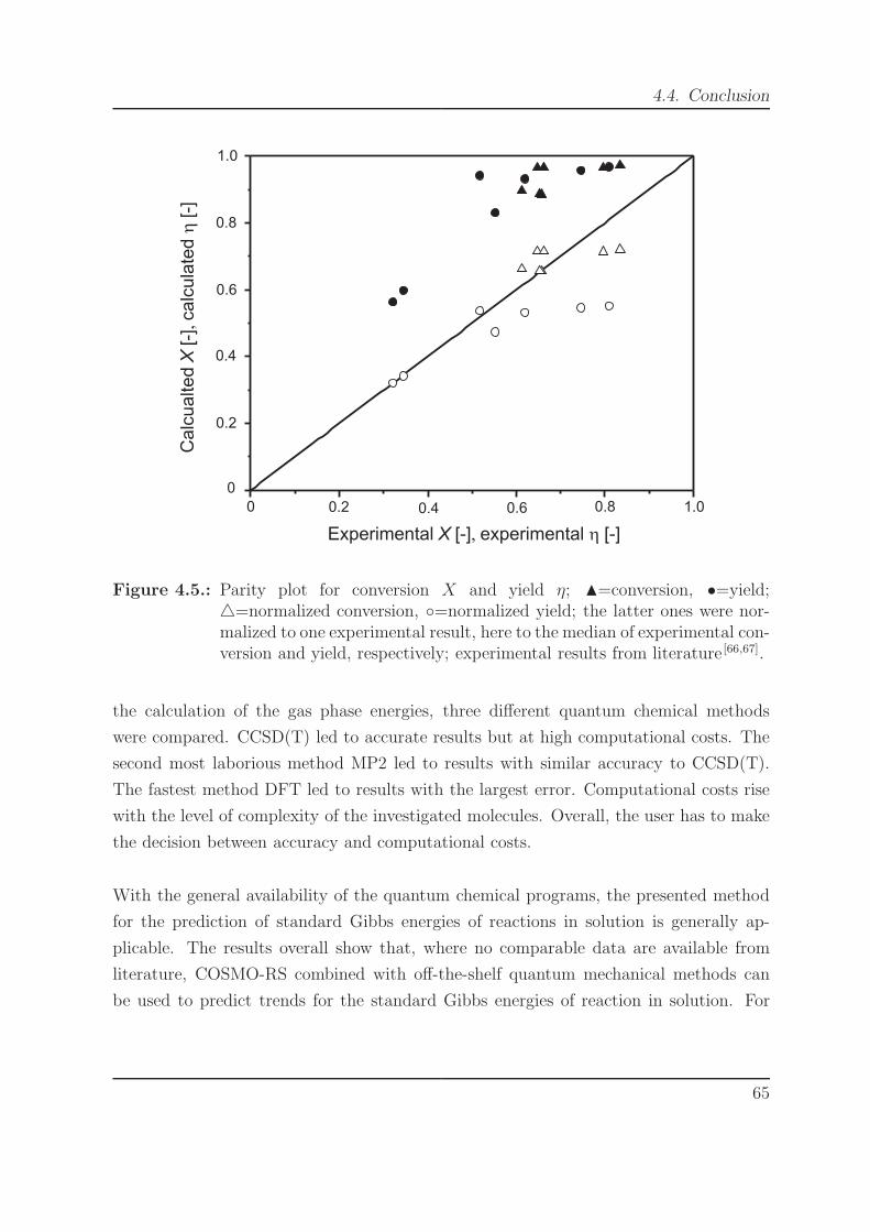
4.4. Conclusion
1.0
0.8
0.6
0.2
0.4
0
1.00.80.60.40.20
Experimental [-] experimental [-], hX
Calc
ualted
[-]
calc
ula
ted
[-]
,h
X
Figure 4.5.: Parity plot for conversion X and yield η; N=conversion, •=yield;△=normalized conversion, ◦=normalized yield; the latter ones were nor-malized to one experimental result, here to the median of experimental con-version and yield, respectively; experimental results from literature [66,67].
the calculation of the gas phase energies, three different quantum chemical methods
were compared. CCSD(T) led to accurate results but at high computational costs. The
second most laborious method MP2 led to results with similar accuracy to CCSD(T).
The fastest method DFT led to results with the largest error. Computational costs rise
with the level of complexity of the investigated molecules. Overall, the user has to make
the decision between accuracy and computational costs.
With the general availability of the quantum chemical programs, the presented method
for the prediction of standard Gibbs energies of reactions in solution is generally ap-
plicable. The results overall show that, where no comparable data are available from
literature, COSMO-RS combined with off-the-shelf quantum mechanical methods can
be used to predict trends for the standard Gibbs energies of reaction in solution. For
65

4. Calculating equilibrium constants
a further refinement and validation of the method more reliable experimental data is
needed.
Moving beyond the prediction of ∆Gsolutionr to a computational solvent screening, a pre-
diction of general trends was possible, exemplarily shown for equilibrium conversion and
product yield. Due to the error in the calculation of ∆Gsolutionr , the absolute values
for conversion and yield differed substantially from experimental values. Correction of
predicted values by scaling with a single experimental point led to quantitative values
within the experimental error. This is often an economically more reasonable way than
an exclusively experimental investigation.
66
5. Combining COSMO-RS with
dynamic modeling for solvent
screening
5.1. Introduction
In the previous chapters, a computational approach to solvent selection was established.
With the method presented so far, a general solvent screening for equilibrium conversion
and yield is possible. But X and η are just the first screening targets. In reality, there
are many more parameters that determine a suitable solvent combination for a reac-
tion. Hence, a further investigation of the reaction system is necessary, typically carried
out experimentally. To reduce the amount of experiments a computational approach is
presented combining ab-initio COSMO-RS calculations with subsequent a posteriori dy-
namic modeling, hence dynamic modeling based on experimental data. With sufficient
experimental data, e.g. the decrease of the initial substrate concentration with time,
mass transfer coefficients and partition coefficients can be modeled. Furthermore, the
dependency of these coefficients on process parameters such as temperature and solubi-
lizer can be modeled.
67
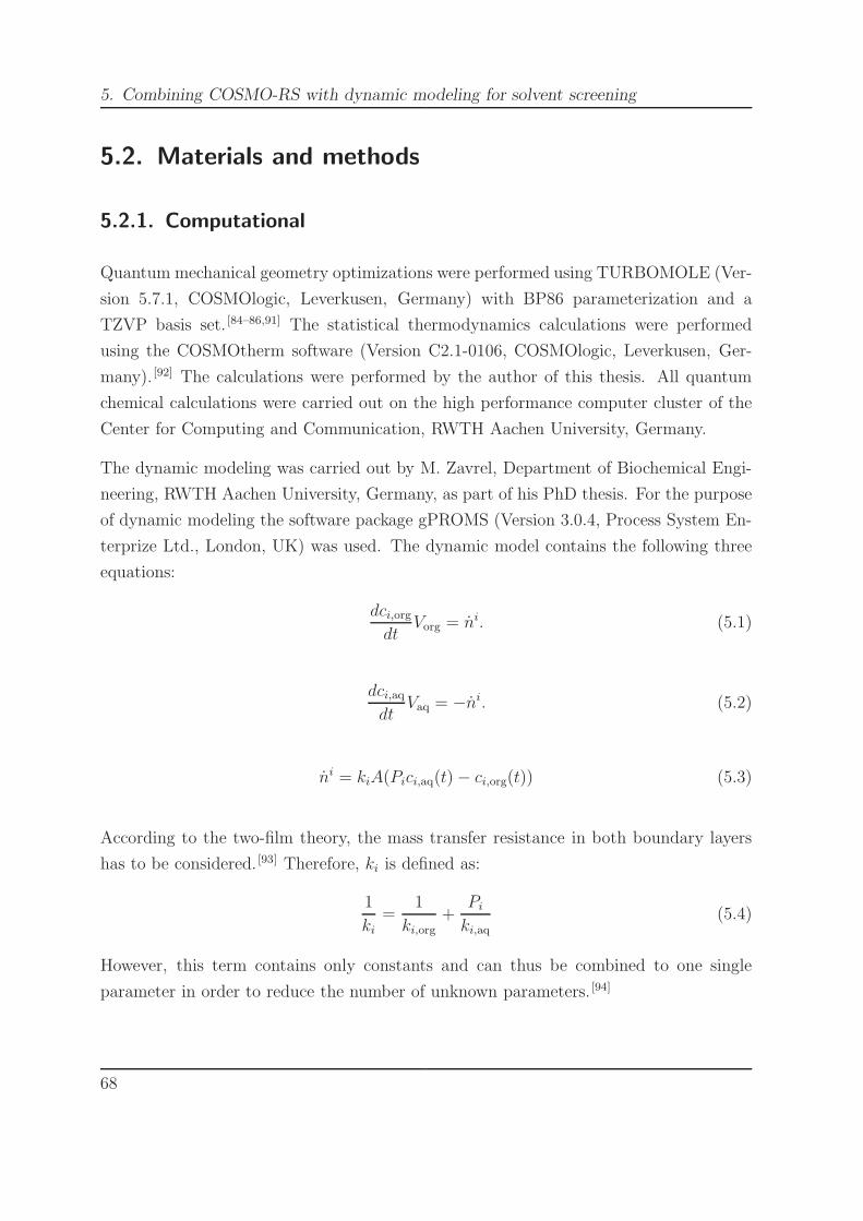
5. Combining COSMO-RS with dynamic modeling for solvent screening
5.2. Materials and methods
5.2.1. Computational
Quantum mechanical geometry optimizations were performed using TURBOMOLE (Ver-
sion 5.7.1, COSMOlogic, Leverkusen, Germany) with BP86 parameterization and a
TZVP basis set. [84–86,91] The statistical thermodynamics calculations were performed
using the COSMOtherm software (Version C2.1-0106, COSMOlogic, Leverkusen, Ger-
many). [92] The calculations were performed by the author of this thesis. All quantum
chemical calculations were carried out on the high performance computer cluster of the
Center for Computing and Communication, RWTH Aachen University, Germany.
The dynamic modeling was carried out by M. Zavrel, Department of Biochemical Engi-
neering, RWTH Aachen University, Germany, as part of his PhD thesis. For the purpose
of dynamic modeling the software package gPROMS (Version 3.0.4, Process System En-
terprize Ltd., London, UK) was used. The dynamic model contains the following three
equations:
dci,org
dtVorg = ni. (5.1)
dci,aq
dtVaq = −ni. (5.2)
ni = kiA(Pici,aq(t) − ci,org(t)) (5.3)
According to the two-film theory, the mass transfer resistance in both boundary layers
has to be considered. [93] Therefore, ki is defined as:
1
ki
=1
ki,org+
Pi
ki,aq(5.4)
However, this term contains only constants and can thus be combined to one single
parameter in order to reduce the number of unknown parameters. [94]
68

5.3. Results and discussion
For the parameter estimation, the initial concentrations, the mass transfer area and
the phase volumes had to be known as well as initial guesses for the mass transfer
coefficients ki and the partition coefficients Pi. Due to the high correlation between the
mass transfer coefficient and the partition coefficient that equals -1 for DMBA and TMB,
the concurrent estimation of both parameters is difficult. That is why in a first step only
the mass transfer coefficient was estimated while for the partition coefficient the value
obtained by HPLC was used (52.5 for DMBA, 89.8 for TMB). [95] In the second step,
both parameters were estimated concurrently.
5.2.2. Experimental
Experiments were carried out by T. Schmidt, Department of Biotechnology, RWTH
Aachen University, Germany, as part of his PhD thesis. [95] Details regarding the specific
reaction set-up can be found in his PhD thesis. For mass transfer experiments the
aqueous phase consisted of a 50 mM KPi buffer and 25 % (v/v) DMF. The latter was
added to increase to solubility of the aromatic compounds. The pH value was set to
8.5 and the ionic strength to 100 mM. The solvents n-hexane and MIBK were used as
organic phases, respectively. The mass transfer experiments were performed at 25◦C
in a continuously stirred tank reactor. Both phases were stirred individually using two
independent stirrers and their volumes were equal. The dynamic measurements were
conducted using a spectrophotometer that recorded the extinction in the aqueous phase.
In all experiments no enzyme was present. For the analysis, high-performance liquid
chromatography (HPLC) was used.
5.3. Results and discussion
5.3.1. Benzaldehyde lyase catalyzed carbon-carbon coupling
So far, bimolecular reactions with partitioning of all reactants were investigated. How-
ever, there are many more types of reactions that are of great industrial interest. The re-
action studied here is the enantioselective carbon-carbon coupling of two 3,5-dimethoxy-
69

5. Combining COSMO-RS with dynamic modeling for solvent screening
benzaldehyde (DMBA) molecules to (R)-3,3’,5,5’-tetramethoxy-benzoin (TMB) using the
enzyme benzaldehyde lyase (BAL, EC 4.1.2.38) (Scheme 5.1). This benzoin formation
is of commercial interest since chiral hydroxy-ketones are important building blocks of
drugs and natural products. [96] A mechanistic model for this reaction has recently been
derived by Zavrel. [97]
BALO
O
O
O
O
O
+O
O
O
OH
O
O
Scheme 5.1: Enantioselective carbon-carbon coupling of 3,5-dimethoxy-benzaldehyde(DMBA) to (R)-3,3’,5,5’-tetramethoxy-benzoin (TMB) catalyzed by BAL.
From a thermodynamic point of view, a well-suited solvent for this reaction type will
continuously push the substrate into the reactive phase while it pulls the product from
the reactive to the non-reactive phase. In other words, the substrate partition coefficient
will be low and the product partition coefficient will be high. Consequently, a factor R
was introduced (equation 5.5), defined as the ratio of the product partition coefficient
divided by the substrate partition coefficient:
R =Pproduct
Psubstrate
. (5.5)
This factor describes the ability of the solvent in the non-reactive phase to shift the
substrate into the reactive phase and to extract the product out of it. There are of course
more parameters that influence maximum conversion and extractable yield obtainable in
a biphasic system, but among these factors, the ratio of partition coefficients R is of great
importance: By increasing R, both conversion and extractable yield are maximized. [98]
A general problem of various reactions of preparative and industrial interest is that their
ratio of partition coefficients is disadvantageous. Furthermore, to use the tool of biphasic
reaction systems effectively for reaction engineering purposes, a distinct knowledge of R is
70
5.3. Results and discussion
required. To obtain reliable data for R, a large number of time-consuming and expensive
experiments are necessary. To overcome the effort of numerous experiments for reaction
optimization in biphasic systems, a systematic approach to solvent selection for biphasic
systems is presented.
The proposed systematic approach to solvent selection combining COSMO-RS with dy-
namic modeling and guided experiments is illustrated in Figure 5.1. Starting point are
quantum mechanical geometry optimizations and COSMO calculations. The subsequent
COSMO-RS (conductor-like screening model for realistic solvation) [70,92,99] calculations
that allow a first ab-initio solvent screening consist of two major steps: the first selection
step is the calculation of liquid-liquid equilibria (LLE). If the solvents do not show a
miscibility gap at reaction temperature with the solvent used are reactive phase, here
water, they are eliminated in the first step.
Those solvents that actually show a miscibility gap with water enter into the second
selection step, the calculation of partition coefficients at infinite dilution and are ranked
accordingly. COSMO-RS can predict general trends for partition coefficients, but the
prediction of absolute values is difficult. [66,90] Hence, an experimental validation is carried
out to check the COSMO-RS solvent ranking.
Experimental data also serves as starting point for the subsequent a posteriori dynamic
modeling. The dynamic model is fitted to experimental data to model partition co-
efficients and mass transfer coefficients. The influence of process parameters such as
temperature and solubilizer content, which can significantly influence the overall mass
transfer, can also be modeled.
71
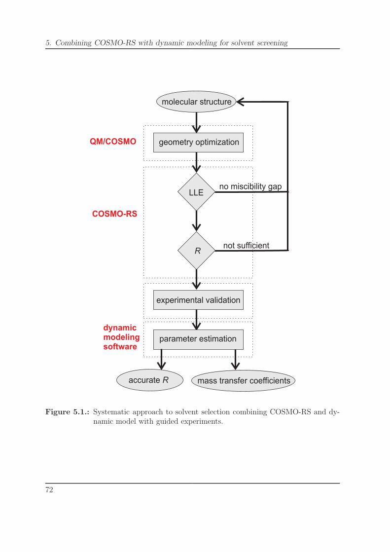
5. Combining COSMO-RS with dynamic modeling for solvent screening
dynamicmodelingsoftware
COSMO-RS
QM/COSMO
not sufficient
no miscibility gapLLE
R
geometry optimization
molecular structure
experimental validation
parameter estimation
mass transfer coefficientsaccurate R
Figure 5.1.: Systematic approach to solvent selection combining COSMO-RS and dy-namic model with guided experiments.
72
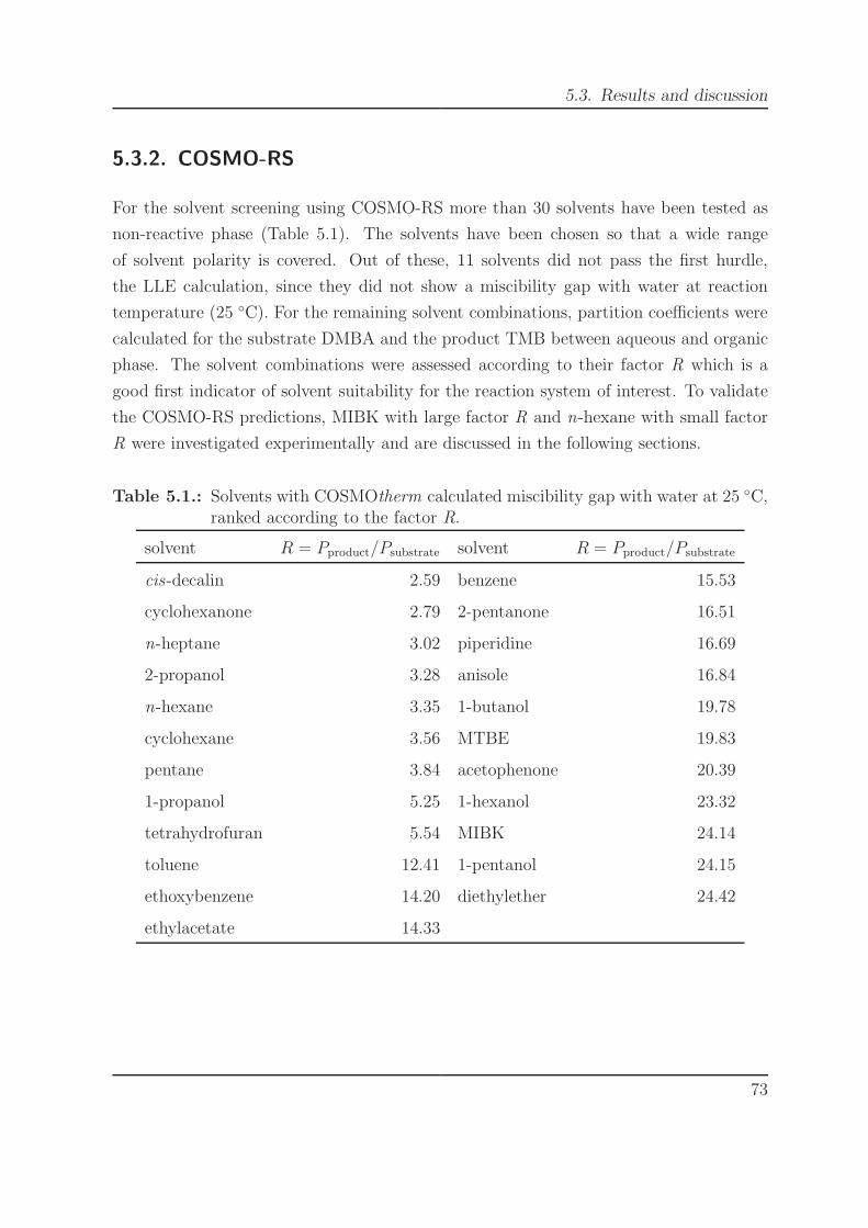
5.3. Results and discussion
5.3.2. COSMO-RS
For the solvent screening using COSMO-RS more than 30 solvents have been tested as
non-reactive phase (Table 5.1). The solvents have been chosen so that a wide range
of solvent polarity is covered. Out of these, 11 solvents did not pass the first hurdle,
the LLE calculation, since they did not show a miscibility gap with water at reaction
temperature (25 ◦C). For the remaining solvent combinations, partition coefficients were
calculated for the substrate DMBA and the product TMB between aqueous and organic
phase. The solvent combinations were assessed according to their factor R which is a
good first indicator of solvent suitability for the reaction system of interest. To validate
the COSMO-RS predictions, MIBK with large factor R and n-hexane with small factor
R were investigated experimentally and are discussed in the following sections.
Table 5.1.: Solvents with COSMOtherm calculated miscibility gap with water at 25 ◦C,ranked according to the factor R.
solvent R = Pproduct/Psubstrate solvent R = Pproduct/Psubstrate
cis-decalin 2.59 benzene 15.53
cyclohexanone 2.79 2-pentanone 16.51
n-heptane 3.02 piperidine 16.69
2-propanol 3.28 anisole 16.84
n-hexane 3.35 1-butanol 19.78
cyclohexane 3.56 MTBE 19.83
pentane 3.84 acetophenone 20.39
1-propanol 5.25 1-hexanol 23.32
tetrahydrofuran 5.54 MIBK 24.14
toluene 12.41 1-pentanol 24.15
ethoxybenzene 14.20 diethylether 24.42
ethylacetate 14.33
73
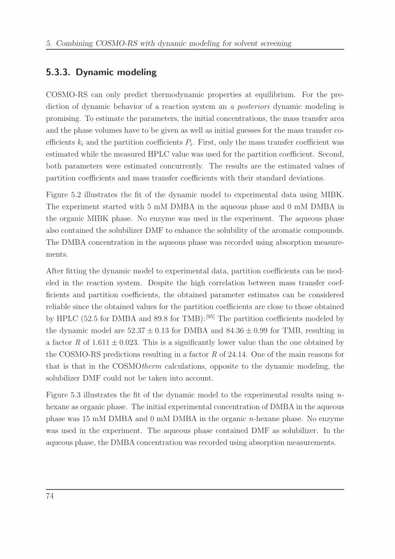
5. Combining COSMO-RS with dynamic modeling for solvent screening
5.3.3. Dynamic modeling
COSMO-RS can only predict thermodynamic properties at equilibrium. For the pre-
diction of dynamic behavior of a reaction system an a posteriori dynamic modeling is
promising. To estimate the parameters, the initial concentrations, the mass transfer area
and the phase volumes have to be given as well as initial guesses for the mass transfer co-
efficients ki and the partition coefficients Pi. First, only the mass transfer coefficient was
estimated while the measured HPLC value was used for the partition coefficient. Second,
both parameters were estimated concurrently. The results are the estimated values of
partition coefficients and mass transfer coefficients with their standard deviations.
Figure 5.2 illustrates the fit of the dynamic model to experimental data using MIBK.
The experiment started with 5 mM DMBA in the aqueous phase and 0 mM DMBA in
the organic MIBK phase. No enzyme was used in the experiment. The aqueous phase
also contained the solubilizer DMF to enhance the solubility of the aromatic compounds.
The DMBA concentration in the aqueous phase was recorded using absorption measure-
ments.
After fitting the dynamic model to experimental data, partition coefficients can be mod-
eled in the reaction system. Despite the high correlation between mass transfer coef-
ficients and partition coefficients, the obtained parameter estimates can be considered
reliable since the obtained values for the partition coefficients are close to those obtained
by HPLC (52.5 for DMBA and 89.8 for TMB): [95] The partition coefficients modeled by
the dynamic model are 52.37 ± 0.13 for DMBA and 84.36 ± 0.99 for TMB, resulting in
a factor R of 1.611 ± 0.023. This is a significantly lower value than the one obtained by
the COSMO-RS predictions resulting in a factor R of 24.14. One of the main reasons for
that is that in the COSMOtherm calculations, opposite to the dynamic modeling, the
solubilizer DMF could not be taken into account.
Figure 5.3 illustrates the fit of the dynamic model to the experimental results using n-
hexane as organic phase. The initial experimental concentration of DMBA in the aqueous
phase was 15 mM DMBA and 0 mM DMBA in the organic n-hexane phase. No enzyme
was used in the experiment. The aqueous phase contained DMF as solubilizer. In the
aqueous phase, the DMBA concentration was recorded using absorption measurements.
74

5.3. Results and discussion
0.0
1.0
2.0
3.0
4.0
5.0
6.0
0 500 1000 1500 2000
time [s]
DM
BA
[mM
]
dynamic model
experimental
Figure 5.2.: Fit of the dynamic model to experimental results; the experiment wasstarted with a DMBA concentration of 5 mM in the aqueous phase, and0 mM in the organic phase (MIBK); the DMBA concentration in the aque-ous phase was recorded using absorption measurements.
0
2
4
6
8
10
12
14
16
0 2000 4000 6000 8000 10000 12000 14000 16000 18000
time [s]
DM
BA
[mM
]
dynamic model
experimental
Figure 5.3.: Fit of the dynamic model to experimental results; the experiment wasstarted with a DMBA concentration of 15 mM in the aqueous phase, and0 mM in the organic phase (n-hexane); the DMBA concentration in theaqueous phase was recorded using absorption measurements.
75
5. Combining COSMO-RS with dynamic modeling for solvent screening
The partition coefficients for DMBA and TMB are in this system dynamically modeled
to be 3.41 ± 0.04 and 0.36 ± 0.01, respectively, R equals 0.106 ± 0.004. COSMO-RS
predictions resulted in a factor R of 3.35. Consequently, for the reaction system of
interest n-hexane is not a suitable organic phase to obtain high yields.
However R can generally be altered by process parameters such as temperature and
volume fraction of the solubilizer DMF. Figure 5.4 illustrates the influence of the tem-
perature on the single partition coefficients and on the factor R. The partition coefficients
show only slight changes whereas the factor R can significantly be increased with increas-
ing temperature.
Figure 5.4.: Influence of temperature on partition coefficients (DMBA: �; TMB: •)and on the R-factor (N).
More pronounced is the effect of the solubilizer DMF shown in Figure 5.5. DMF in-
creases the equilibrium concentration of both reactants in the aqueous phase. However,
the decrease of the product partition coefficient is more pronounced than the substrate
partition coefficient. As a result, the factor R can be increased by reducing the amount
of solubilizer in the aqueous phase. Concluding, a process using n-hexane as extraction
76

5.3. Results and discussion
solvent should be operated at high temperatures and with as little as possible solubilizer
DMF.
Figure 5.5.: Influence of the solubilizer DMF on partition coefficients (DMBA: �;TMB: •) and on the R-factor (N).
If the factor R of MIBK and n-hexane are compared it becomes obvious that, despite the
fact that their absolute values are not predicted accurately, the overall trend is verified.
The predicted ratio of the R factors of MIBK and n-hexane by COSMO-RS is 7.16,
while the ratio of R factors determined by the dynamic modeling is 14.63. Consequently,
MIBK turned out to be a more suitable solvent for the reaction in terms of partition
coefficients.
The mass transfer coefficients in MIBK at 298 K for the substrate DMBA with a 95%
confidence interval are modeled to be kDMBA = 5.39 · 10−07 ms± 1.33 · 10−09 m
s. For the
product TMB the mass transfer coefficients with a 95% confidence interval are estimated
to be k(TMB) = 2.81 · 10−07 ms±3.33 · 10−09 m
s. This seems reasonable since the substrate
DMBA should diffuse faster through the interface than the larger product TMB.
Certainly, there are many more parameters than partition coefficients and mass transfer
coefficients that have an influence on the final solvent choice for an industrial process,
77
5. Combining COSMO-RS with dynamic modeling for solvent screening
such as enzyme stability, safety aspects, price and availability. Mostly, solvent selection
in industry is a compromise.
5.4. Conclusion
A systematic approach to solvent selection for biphasic aqueous-organic reactions was
presented. The model reaction was the enantioelective carbon-carbon coupling of two
3,5-dimethoxy-benzaldehyde (DMBA) molecules to (R)-3,3’,5,5’-tetramethoxy-benzoin
(TMB).
In the first step, COSMO-RS was used as a fast and effective solvent screening tool. The
accuracy of the calculated results was sufficient for a first solvent screening. Although
no reliable absolute values could be predicted, the method was nevertheless a valuable
tool at least as long as the solubilizer is neglected. The second step, where a dynamic
model was fitted to experimental data, lead to a more detailed and exact study of the
model system. Furthermore, not only the mass transfer coefficients and the partition
coefficients could be modeled but also the dependency on process parameters such as
temperature and solubilizer content, which might significantly affect the mass transfer
as demonstrated.
78
6. Conclusion and Outlook
Solvent selection is a key requirement for the successful implementation of environmen-
tally benign but economically competitive processes in chemical production. Up to date,
a suitable solvent for an industrial process is chosen by many time-consuming and cost-
intensive experiments. For multiphase systems the interaction of the phases multiplies
the complexity and the expenses for the choice of the best combination. To minimize
the cost of experimental work, to enlarge the dataspace but also to reduce the environ-
mental impact, a computational solvent screening procedure based on thermodynamic
properties is a promising alternative (Figure 6.1).
The basic target reaction system investigated in this thesis was the biphasic reaction sys-
tem with one reactive phase. Due to the possibility of integrating downstream processing
and facilitating product separation, biphasic reaction systems are of high industrial rel-
evance. Nevertheless, their exact mathematical description is complex. And the further
combination of biphasic systems with a reaction taking place in the reactive phase renders
an additional challenge.
Suitable model reactions for biphasic systems are biocatalytic reactions, as they offer
the advantages of ideal selectivity towards the product. Furthermore, they are strongly
limited by thermodynamics. Two biocatalytic reactions were examined here: On the
one hand the enzymatic substrate coupled cofactor regeneration where acetophenone
is enantioselectively reduced to (R)-phenylethanol while 2-propanol is oxidized to ace-
tone, on the other hand the enzymatic enantioselective carbon-carbon coupling of two
3,5-dimethoxy-benzaldehyde (DMBA) molecules to (R)-3,3’,5,5’-tetramethoxy-benzoin
(TMB).
In order to judge the potential of different biphasic reaction systems, conversion X and
yield η were applied as dimensionless measures for reaction progress and maximum re-
79
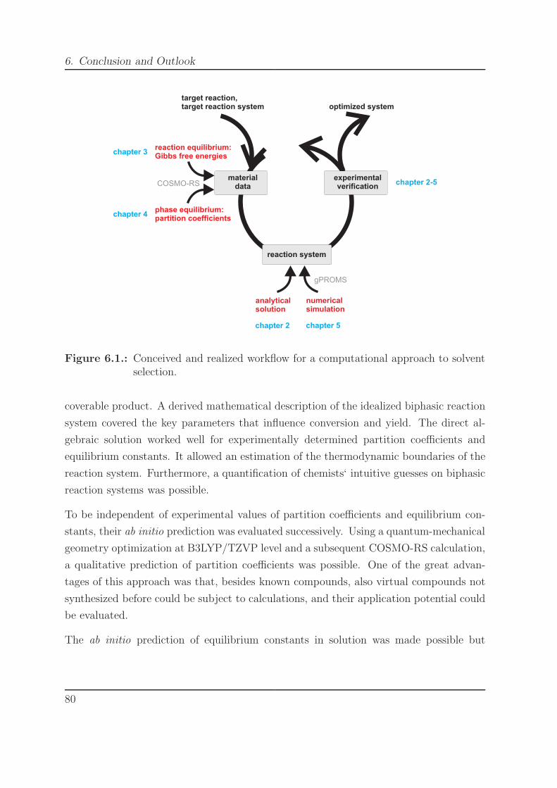
6. Conclusion and Outlook
gPROMS
COSMO-RS
target reaction,target reaction system
experimentalverification
materialdata
reaction system
phase equilibrium:partition coefficients
reaction equilibrium:Gibbs free energies
analyticalsolution
numericalsimulation
optimized system
chapter 2-5
chapter 5chapter 2
chapter 3
chapter 4
Figure 6.1.: Conceived and realized workflow for a computational approach to solventselection.
coverable product. A derived mathematical description of the idealized biphasic reaction
system covered the key parameters that influence conversion and yield. The direct al-
gebraic solution worked well for experimentally determined partition coefficients and
equilibrium constants. It allowed an estimation of the thermodynamic boundaries of the
reaction system. Furthermore, a quantification of chemists‘ intuitive guesses on biphasic
reaction systems was possible.
To be independent of experimental values of partition coefficients and equilibrium con-
stants, their ab initio prediction was evaluated successively. Using a quantum-mechanical
geometry optimization at B3LYP/TZVP level and a subsequent COSMO-RS calculation,
a qualitative prediction of partition coefficients was possible. One of the great advan-
tages of this approach was that, besides known compounds, also virtual compounds not
synthesized before could be subject to calculations, and their application potential could
be evaluated.
The ab initio prediction of equilibrium constants in solution was made possible but
80

proved to be much more complicated than the partition coefficient calculation. A gener-
ally applicable workflow was set up, applied here to the reduction of differently substi-
tuted ketones in toluene. In the calculations, the first step was a quantum-mechanical
geometry optimization at B3LYP/TZVP level. For the subsequent single-point calcu-
lations, different quantum-chemical methods have been evaluated, in fact, in the order
of increasing complexity and increasing computational cost: DFT (density functional
theory), MP2 (2nd-order Møller–Plesset perturbation theory) and CC (coupled-cluster
theory). Fortunately, for the equilibrium constant calculation, MP2 as being a method
with medium complexity and medium computational demand led to results with simi-
lar accuracy as CC, the most complex and computationally most demanding method.
Overall, this allowed a prediction of equilibrium constants or standard Gibbs energies
of reaction in solution, respectively. This is especially important for equilibrium limited
reactions.
For an evaluation of the overall process, a reduction to the dimensionless figures conver-
sion X and yield η was made on the basis of ab initio data. Although at some stages
deviations between experimental and calculated partition coefficients or equilibrium con-
stants occurred, the overall results for conversion X and yield η were very promising.
The ranking according to the ab initio predictions was in line with the experimental
data. Normalizing to one experimental data point rendered the absolute data to mirror
the experimental data fairly well. The investigations did not only reduce the amount
of experiments but also led to a deeper understanding of reactions in biphasic reactions
systems.
In order to benchmark the developed approach to computational solvent screening in
biphasic reaction systems and to increase the overall predictive power of the method,
reliable experimental data is needed. This is important for the testing and adjusting
of the developed mathematical description and for extending this approach to other
reactions, for example condensation reactions.
Reliable experimental data is also needed to verify and refine the computational tools
used within this thesis such as COSMO-RS. The method leads to remarkably good re-
sults for molecules that do not have a too large structural variety. If more sophisticated
substrates are to be considered in the solvents selection process, COSMO-RS still runs
81

6. Conclusion and Outlook
into problems. This has been shown in a cooperation with Shell Global Solutions, Ams-
terdam, The Netherlands. In this project, activity coefficients of about 2000 ionic liquids
have been screened for an industrial application. It could be shown that for ionic liquids
the ab initio prediction of activity coefficients using COSMO-RS works very well, but
the prediction of liquid-liquid-equilibria is still difficult. Since the calculation of the lat-
ter is always the first step in partition coefficient calculation, large errors might be the
consequence. Up to date, the structural diversity of ionic liquids is not satisfactorily cov-
ered by COSMO-RS, especially the various intermolecular interactions. Moreover, first
approaches to the prediction of polymeric properties are established but still challenging,
and there is still room for further improvement.
Reliable experimental data is also needed to enhance the calculation of equilibrium con-
stants of reactions in solution. Here, solvent dependent equilibrium constants for different
types of reaction would be of great importance. With a further development of computer
power, complex quantum-mechanical methods might become more and more attractive
in the future.
For the determination of reliable experimental data, an automatization and miniaturiza-
tion of the experiments would be a great advantage. Especially for the measurement of
partition coefficients, the combination with robotics would have a major impact on the
further development of the method and the computational tools.
The analytical mathematical description of the biphasic reaction system with one reactive
phase is only accurate for strongly idealized reaction systems. To improve the method
and to be able to treat non-ideal reaction systems, the combination with numerical
simulation tools is the logical consequence. Briefly touched upon within this thesis,
the combination with numerical simulation tools also enables the treatment of dynamic
effects and does not necessarily stay with the static picture. For example, it allows a
treatment of solubilizer which up to date cannot be treated satisfactorily using COSMO-
RS. For the future, this might also link thermodynamic and kinetic investigations of
reaction systems.
One of the major goals on the way towards computational solvent screening is an au-
tomated computational approach as this enables a fast and effective screening. In a
cooperation with Bayer MaterialScience, Leverkusen, Germany within a project at the
82

CAT Catalytic Center at RWTH Aachen University, Germany, an automated solvent
screening method was set up. For an industrial application, in total about 20000 sol-
vent combinations could be investigated computationally. Including this approach in a
software tool would enable fast screening processes.
Extending the idea of a computational solvent screening to other industrial problems
such as crystallization is also possible. In a cooperation with a leading European phar-
maceutical company, a solvent screening for crystallization processes has been carried
out. First results look promising and raise expectations for future investigations.
Summarizing, the modeling of fluid phases is very complex and still deserves intensive
study by interdisciplinary research teams. For the future, more experimental data are
needed to optimize and benchmark computational tools and derived computational meth-
ods. The overall goal would be to establish a quantitative structure-activity relationship.
The future development of more computer power is probably a major step towards an
effective usage of computational tools. The first important steps have been made and
have yielded promising results.
83

6. Conclusion and Outlook
84
Bibliography
[1] H. Boerhaave, Elementa Chemiae, G. Cavelier, Paris, 1733, 1, p. 588.
[2] G. A. Lindeboom, Herman Boerhaave - The Man and his Work, Methuen, London,
1968.
[3] C. Reichardt, Solvents and solvent effects in organic chemistry, VCH, Weinheim,
1988, 2nd ed.
[4] W. Keim, Green Chem. 2003, 5, 105-111.
[5] R. V. Chaudhari, P. L. Mills, Chem. Eng. Sci. 2004, 59, 5337–5344.
[6] T. Prinz, W. Keim, B. Driessen-Hoelscher, Ang. Chem. Int. Ed. Engl. 1996, 35, 15,
1708-1710.
[7] P. J. Halling, Biotech. Adv. 1987, 5, 47–87.
[8] B. Cornils, W. A. Herrmann, Eds., Applied homogeneous catalysis with organometal-
lic compounds,., Wiley- VCH, Weinheim, 2002, 2nd ed.
[9] B. Cornils, W. A. Herrmann, I. T. Horvath, W. Leitner, S. Mecking, H. Olivier-
Bourbigou, D. Vogt, Eds., Multiphase homogeneous catalysis, Wiley-VCH, Wein-
heim, 2005.
[10] A. J. J. Straathof, Thermodynamics for biochemical engineers, Course book, Murren,
Switzerland, 2005, Chap. Thermodynamics in multiphase biocatalysis.
[11] H. Groger, W. Hummel, C. Rollmann, F. Chamouleau, H. Husken, H. Werner,
C. Wunderlich, K. Abokitse, K. Drauz, S. Buchholz, Tetrahedron 2004, 60, 633–640.
85
Bibliography
[12] M. V. Filho, T. Stillger, M. Muller, A. Liese, C. Wandrey, Angew. Chem. Int. Ed.
2003, 42, 2993–2996.
[13] H. Klein, R. Jackstell, M. Beller, Chem. Commun. 2005, 2283–2285.
[14] O. Hernandez-Justiz, R. Fernandez-Lafuente, M. Terreni, J. M. Guisan, Biotechnol.
Bioeng. 1998, 59, 73–79.
[15] M. Bauer, H. Griengl, W. Steiner, Enzyme Microb. Tech. 1999, 24, 514–522.
[16] V. Sandford, M. Breuer, B. Hauer, P. Rogers, B. Rosche, Biotechnol. Bioeng. 2005,
91, 190-198.
[17] D. J. Adams, D. J. Cole-Hamilton, E. G. Hope, P. J. Pogorzelec, A. M. Stuart, J.
Organomet. Chem. 2004, 689, 1413–1417.
[18] P. J. Dyson, Chimia 2005, 59, 66–71.
[19] M. F. Eckstein, M. V. Filho, A. Liese, U. Kragl, Chem. Commun. 2004, 1084–1085.
[20] H. Pfrunder, M. Amidjojo, U. Kragl, D. Weuster-Botz, Angew. Chem. Int. Ed.
2004, 43, 4529–4531.
[21] S. G. Cull, J. D. Holbrey, V. Vargas-Mora, K. R. Seddon, G. J. Lye, Biotechnol.
Bioeng. 2000, 69, 227-233.
[22] A. Bosmann, B. Francio, E. Janssen, M. Solinas, W. Leitner, P. Wasserscheid,
Angew. Chem. 2001, 113, 2769–2699.
[23] M. T. Reetz, W. Wiesenhofer, G. Francio, W. Leitner, Chem. Commun. 2002,
992–993.
[24] W. F. Willeman, R. Neuhofer, I. Wirth, P. Pochlauer, A. J. J. Straathof, J. J.
Heijnen, Biotechnol. Bioeng. 2002, 79, 154-164.
[25] S. Morikawa, T. Nakai, Y. Yasohara, H. Nanba, N. Kizaki, J. Hasegawa, Biosci.
Biotechnol. Biochem. 2005, 69, 544-552.
[26] S. Chen, P. C. Engel, Enzyme Microb. Technol. 2007, 40, 1407-1411.
86
Bibliography
[27] B. Rosche, M. Breuer, B. Hauer, P. L. Rogers, Biotechnol. Bioeng. 2004, 86, 788-
794.
[28] K. Lucas, Molecular models for fluids, Cambridge University Press, 2007.
[29] C. J. Cramer, Essentials of Computational Chemistry - Theories and Models, John
Wiley and Sons Ltd., 2004, 2nd ed.
[30] J. Tomasi, B. Mennucci, R. Cammi, Chem. Rev. 2005, 105, 2999-3093.
[31] M. Born, Z. Phys. 1920, 1, 45-48.
[32] J. Tomasi, M. Persico, Chem. Rev. 1994, 94, 2017-2094.
[33] C. J. Cramer, D. G. Truhlar, Chem. Rev. 1999, 99, 2161-2200.
[34] M. Orozco, F. J. Luque, Chem. Rev. 2000, 100, 4187-4225.
[35] W. Kutzelnigg, Einfuhrung in die Theoretische Chemie, Vol. 1 + 2., VCH, Wein-
heim, 1992.
[36] A. Szabo, N. S. Ostlund, Modern Quantum Chemistry, Dover Publ. Inc., New York,
1996.
[37] W. Bobrowicz, W. Goddard, H. F. Schaefer, Methods of Electronic Structure Theory,
Vol. III, Modern Theoretical Chemistry Plenum, New York, 1977, Chap. The Self-
Consistent Field Equation for Generalized Valence Bond and Open-Shell Hartree-
Fock Wave Functions, pp. 79–126.
[38] C. Møller, M. S. Plesset, Phys. Rev. 1934, 46, 618-622.
[39] J. Cızek, Adv. Chem. Phys. 1969, 14, 35-88.
[40] J. A. Pople, M. Head-Gordon, K. Raghavachari, J. Chem. Phys. 1987, 87, 5968-
5975.
[41] M. Head-Gordon, J. A. Pople, M. J. Frisch, Chem. Phys. Lett. 1988, 153, 503-506.
[42] M. J. Frisch, M. Head-Gordon, J. A. Pople, Chem. Phys. Lett. 1990, 166, 275-280.
[43] M. J. Frisch, M. Head-Gordon, J. A. Pople, Chem. Phys. Lett. 1990, 166, 281-289.
[44] M. Head-Gordon, T. Head-Gordon, Chem. Phys. Lett. 1994, 220, 122-128.
87
Bibliography
[45] R. Krishnan, J. A. Pople, Int. J. Quant. Chem. 1978, 14, 91-100.
[46] R. J. Bartlett, J. Phys. Chem. 1989, 93, 1697-1708.
[47] J. A. Pople, R. Krishnan, H. B. Schlegel, J. S. Binkley, Int. J. Quant. Chem. 1978,
14, 545-560.
[48] R. J. Bartlett, G. D. Purvis, Int. J. Quant. Chem. 1978, 14, 561-581.
[49] W. Kohn, L. J. Sham, Phys. Rev. 1965, 140, A1133-A1138.
[50] P. Hohenberg, W. Kohn, Phys. Rev. 1964, 136, B864-B871.
[51] A. Klamt, G. Schuurmann, J. Chem. Soc. Perk. T 2 1993, 799–805.
[52] D. M. Dolney, G. D. Hawkins, P. Winget, D. A. Liotard, C. J. Cramer, D. G.
Truhlar, J. Comput. Chem. 2000, 21, 340-366.
[53] A. Klamt, V. Jonas, T. Burger, J. C. W. Lohrenz, J. Phys. Chem. A 1998, 102,
5074–5085.
[54] A. Schafer, A. Klamt, D. Sattel, J. C. W. Lohrenz, F. Eckert, Phys. Chem. Chem.
Phys. 2000, 2, 2187–2193.
[55] A. Fredenslund, R. L. Jones, J. M. Prausnitz, AIChE J. 1975, 21, 1086-1099.
[56] J. Gmehling, Fluid Phase Equilibr 1998, 144, 37-47.
[57] U. Weidlich, J. Gmehling, Ind. Eng. Chem. Res. 1987, 26, 7, 1372-1381.
[58] R. Gani, Comp. Chem. Eng. 2004, 28, 2441-2457.
[59] H. E. Gonzalez, J. Abildskov, R. Gani, Fluid Phase Equilibr. 2007, 261, 199-204.
[60] J. V. Sengers, R. F. Kayser, C. F. Peters, J. H. White Jr., Eds., Equations of State
for Fluids and Fluid Mixtures, Elsevier, Amsterdam, 2000.
[61] K. Binder, J. Horbach, W. Kob, W. Paul, F. Varnik, J. Phys.: Condens. Matter.
2004, 16, 429-453.
[62] M. Sprik, J. Phys.: Condens. Matter 1996, 8, 9405-9409.
88
Bibliography
[63] M. H. Kalos, P. Whitlock, Monte-Carlo Methods, I: Basics., Wiley-VCH, New York,
1986.
[64] J. B. Anderson, Reviews in Computational Chemistry, Wiley-VCH, New York, 1999.
[65] M. F. Eckstein, Alcohol dehydrogenase catalysed reductions in nonconventional me-
dia, PhD thesis, University of Rostock, Germany, 2004.
[66] M. F. Eckstein, M. Peters, J. Lembrecht, A. C. Spiess, L. Greiner, Adv. Synth. Catal.
2006, 348, 1591-1596.
[67] M. F. Eckstein, J. Lembrecht, J. Schumacher, M. Peters, C. Roosen, L. Greiner,
W. Eberhard, A. C. Spiess, W. Leitner, U. Kragl, Adv. Synth. Catal. 2006, 348,
1597-1604.
[68] R. V. Wisman, F. G. de Vries, B. J. Deelman, H. J. Heeres, Org. Process Res. Dev.
2006, 10, 423-429.
[69] L. Greiner, S. Laue, A. Liese, C. Wandrey, Chem. Eur. J. 2006, 12, 1818-1823.
[70] A. Klamt, J. Phys. Chem. 1995, 99, 2224–2235.
[71] A. Klamt, Cosmo-RS: From Quantum Chemistry to Fluid Phase Thermodynamics
and Drug Design., Elsevier, Amsterdam, 2005.
[72] J. W. Sørensen, W. Arlt, Liquid–Liquid Equilibrium Data Collection: Binary Sys-
tems, 1, DECHEMA, Frankfurt/Main, 1979.
[73] J. R. Matos, C. H. Wong, J. Org. Chem. 1986, 51, 2388–2389.
[74] S. I. Suye, K. Kamiya, T. Kawamoto, A. Tanaka, Biocatal. Biotransfor. 2002, 20,
23–28.
[75] M. Eckstein, T. Daußmann, U. Kragl, Biocatal. Biotransfor. 2004, 22, 89–96.
[76] M. Heinemann, A. Kummel, R. Giesen, M. Ansorge-Schumacher, J. Buchs, Biocatal.
Biotransfor. 2003, 21, 115-121.
[77] S. T. Lin, S. I. Sandler, Ind. Eng. Chem. Res. 2002, 41, 899–913.
[78] L. Barcza, E. Foldeaki, Acta Chim. Acad. Sci. Hungar. 1977, 95, 247–252.
89
Bibliography
[79] E. C. Voutsas, H. Stamatis, F. N. Kolisis, D. Tassios, Biocatal. Biotransfor. 2002,
20, 101–109.
[80] F. Eckert, A. Klamt, AIChE J. 2002, 48, 369–385.
[81] L. J. Bruce, A. J. Daugulis, Biotechnol. Progr. 1991, 7, 116–124.
[82] J. B. Foresman, A. E. Frisch, Exploring Chemistry with Electronic Structure Meth-
ods, Gaussian Inc., Pittsburgh, 1996, 2nd ed.
[83] M. J. Frisch, G. W. Trucks, H. B. Schlegel, G. E. Scuseria, M. A. Robb, J. R. Cheese-
man, J. A. J. Montgomery, T. Vreven, K. N. Kudin, J. C. Burant, J. M. Millam,
S. S. Iyengar, J. Tomasi, V. Barone, B. Mennucci, M. Cossi, G. Scalmani, N. A.
R. N. G. A. Petersson, H. Nakatsuji, M. Hada, M. Ehara, K. Toyota, R. Fukuda,
J. Hasegawa, M. Ishida, T. Nakajima, Y. Honda, O. Kitao, H. Nakai, M. Klene,
X. Li, J. E. Knox, H. P. Hratchian, J. B. Cross, V. Bakken, C. Adamo, J. Jaramillo,
R. Gomperts, R. E. Stratmann, O. Yazyev, A. J. Austin, R. Cammi, C. Pomelli,
J. W. Ochterski, P. Y. Ayala, K. Morokuma, G. A. Voth, P. Salvador, J. J. Dan-
nenberg, V. G. Zakrzewski, S. Dapprich, A. D. Daniels, M. C. Strain, O. Farkas,
D. Malick, A. D. Rabuck, K. Raghavachari, J. B. Foresman, J. V. Ortiz, Q. Cui,
A. G. Baboul, S. Clifford, J. Cioslowski, B. B. Stefanov, G. Liu, A. Liashenko,
P. Piskorz, I. Komaromi, R. L. Martin, D. J. Fox, T. Keith, M. A. Al-Laham,
C. Peng, A. Nanayakkara, M. Challacombe, P. M. W. Gill, B. Johnson, W. Chen,
M. W. Wong, C. Gonzalez, J. A. Pople, Gaussian 03, Revision C.02.
[84] R. Ahlrichs, M. Bar, M. Haser, H. Horn, H. Kolmel, Chem. Phys. Lett. 1989, 162,
165-169.
[85] M. Haser, R. Ahlrichs, J. Comput. Chem. 1989, 10, 104-111.
[86] H. Horn, H. Weiss, M. Haser, M. Ehrig, R. Ahlrichs, J. Comput. Chem. 1991, 12,
1058-1064.
[87] F. Eckert, A. Klamt, Cosmotherm, Version C2.1, Release 01.05, COSMOlogic
GmbH & Co. KG, Leverkusen, Germany, 2005.
[88] T. E. Daubert, R. P. Danner, Physical and Thermodynamical Properties of Pure
Chemicals, Taylor and Francis, Washington, 1998.
90
Bibliography
[89] H. Adkins, R. M. Elofson, A. G. Rossow, C. C. Robinson, J. Am. Chem. Soc. 1949,
3622–3629.
[90] A. C. Spiess, W. Eberhard, M. Peters, M. F. Eckstein, L. Greiner, J. Buchs, Chem.
Eng. Proc. 2008, 47, 1034-1041.
[91] O. Treutler, R. Ahlrichs, J. Chem. Phys. 1995, 102, 346-354.
[92] F. Eckert, A. Klamt, Cosmotherm, Version C2.1, Release 01.06, COSMOlogic
GmbH & Co. KG, Leverkusen, Germany, 2006.
[93] W. K. Lewis, W. G. Whitman, Ind. Eng. Chem. 1924, 16, 1215-1220.
[94] J. Møllerup, E. Hansen, J. Chromatogr. A 1998, 827, 235-239.
[95] T. W. Schmidt, Experimentelle Analyse, Modellierung und biochemische Charakter-
isierung von Ein- und Zweiphasenreaktionen fur die technische Biokatalyse, PhD
thesis, RWTH Aachen University, 2008.
[96] A. S. Demir, H. Hamamci, O. Sesenoglu, F. Aydogan, D. Capanoglu, R. Nesli-
hanoglu, Tetrahedron Asymm. 2005, 12, 1953-1956.
[97] M. Zavrel, T. Schmidt, C. Michalik, M. Ansorge-Schumacher, W. Marquardt,
J. Buchs, A. C. Spiess, Biotechnol. Bioeng. 2008, 101, 27-38.
[98] M. Peters, M. F. Eckstein, G. Hartjen, A. C. Spiess, W. Leitner, L. Greiner, Ind.
Eng. Chem. Res. 2007, 46, 7073-7078.
[99] A. Klamt, Encyclopedia of Computational Chemistry, John Wiley and Sons Ltd,
New York, 1996.
91

Bibliography
92

Appendix
93


A. Computational details
A.1. Hardware
All quantum chemical calculations were carried out on the high performance computer
cluster of the Center for Computing and Communication, RWTH Aachen University,
Germany.
A.2. Software
The software packages and tools used for the calculations within this thesis are the
following:
• Maple 10 (The Mathworks)
• GaussView (Version 3.09)
• Gaussian (Version 03)
• TURBOMOLE (Versions 5.7.1/5.8)
• COSMOtherm (Versions C2.1-0104/C2.1-0105/C2.1-0106)
• gPROMS (Version 3.0.4)
Computational details can be found in the respective chapters.
95
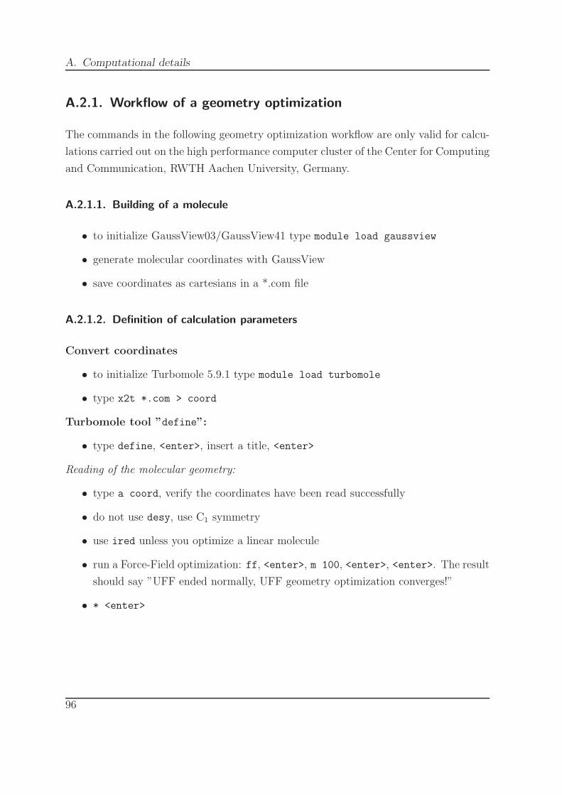
A. Computational details
A.2.1. Workflow of a geometry optimization
The commands in the following geometry optimization workflow are only valid for calcu-
lations carried out on the high performance computer cluster of the Center for Computing
and Communication, RWTH Aachen University, Germany.
A.2.1.1. Building of a molecule
• to initialize GaussView03/GaussView41 type module load gaussview
• generate molecular coordinates with GaussView
• save coordinates as cartesians in a *.com file
A.2.1.2. Definition of calculation parameters
Convert coordinates
• to initialize Turbomole 5.9.1 type module load turbomole
• type x2t *.com > coord
Turbomole tool ”define”:
• type define, <enter>, insert a title, <enter>
Reading of the molecular geometry:
• type a coord, verify the coordinates have been read successfully
• do not use desy, use C1 symmetry
• use ired unless you optimize a linear molecule
• run a Force-Field optimization: ff, <enter>, m 100, <enter>, <enter>. The result
should say ”UFF ended normally, UFF geometry optimization converges!”
• * <enter>
96

A.2. Software
Definition of the basis set:
• type b <enter> all TZVP <enter> to use Ahlrichs TZVP basis for all atoms
• * <enter>
Definition of MOs:
• type eht <enter> to use the Extended Huckel Theory
• enter charge if necessary
• press <enter> after all questions to use default values
Definition of the calculation parameters:
• for a DFT calculation with the BP functional and RI approximation type
dft <enter> on <enter> <enter> ri <enter> jbas <enter> b <enter>
all def-TZVP <enter> * <enter> on <enter> <enter>
• type * <enter> to finish the Turbomole tool "define", check ”define ended nor-
mally”
Turbomole tool ”cosmoprep”:
• type cosmoprep
• press <enter> eight times
• type r all o
• type * <enter>
• enter a name for the *.ccf file
97

A. Computational details
98
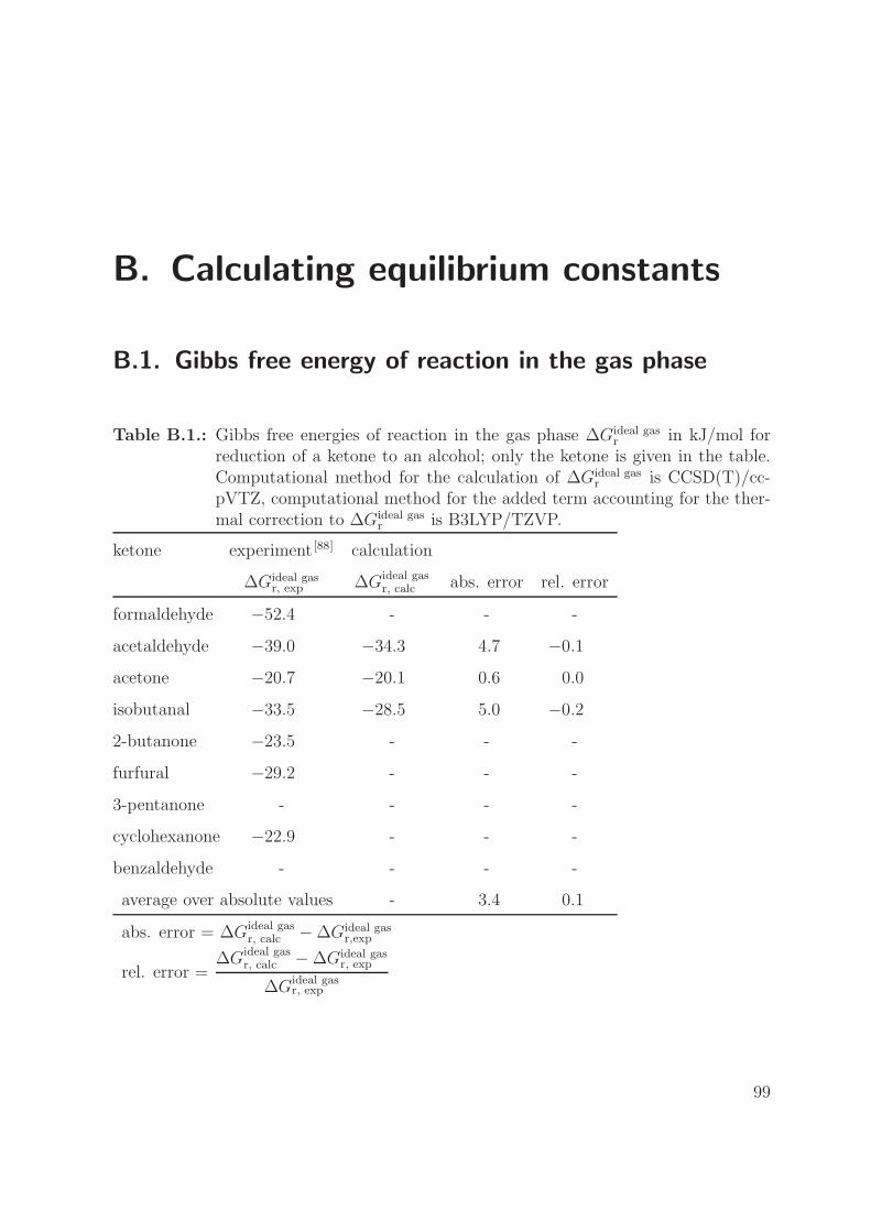
B. Calculating equilibrium constants
B.1. Gibbs free energy of reaction in the gas phase
Table B.1.: Gibbs free energies of reaction in the gas phase ∆Gideal gasr in kJ/mol for
reduction of a ketone to an alcohol; only the ketone is given in the table.Computational method for the calculation of ∆Gideal gas
r is CCSD(T)/cc-pVTZ, computational method for the added term accounting for the ther-mal correction to ∆Gideal gas
r is B3LYP/TZVP.
ketone experiment [88] calculation
∆Gideal gasr, exp ∆Gideal gas
r, calc abs. error rel. error
formaldehyde −52.4 - - -
acetaldehyde −39.0 −34.3 4.7 −0.1
acetone −20.7 −20.1 0.6 0.0
isobutanal −33.5 −28.5 5.0 −0.2
2-butanone −23.5 - - -
furfural −29.2 - - -
3-pentanone - - - -
cyclohexanone −22.9 - - -
benzaldehyde - - - -
average over absolute values - 3.4 0.1
abs. error = ∆Gideal gasr, calc − ∆Gideal gas
r,exp
rel. error =∆Gideal gas
r, calc − ∆Gideal gasr, exp
∆Gideal gasr, exp
99
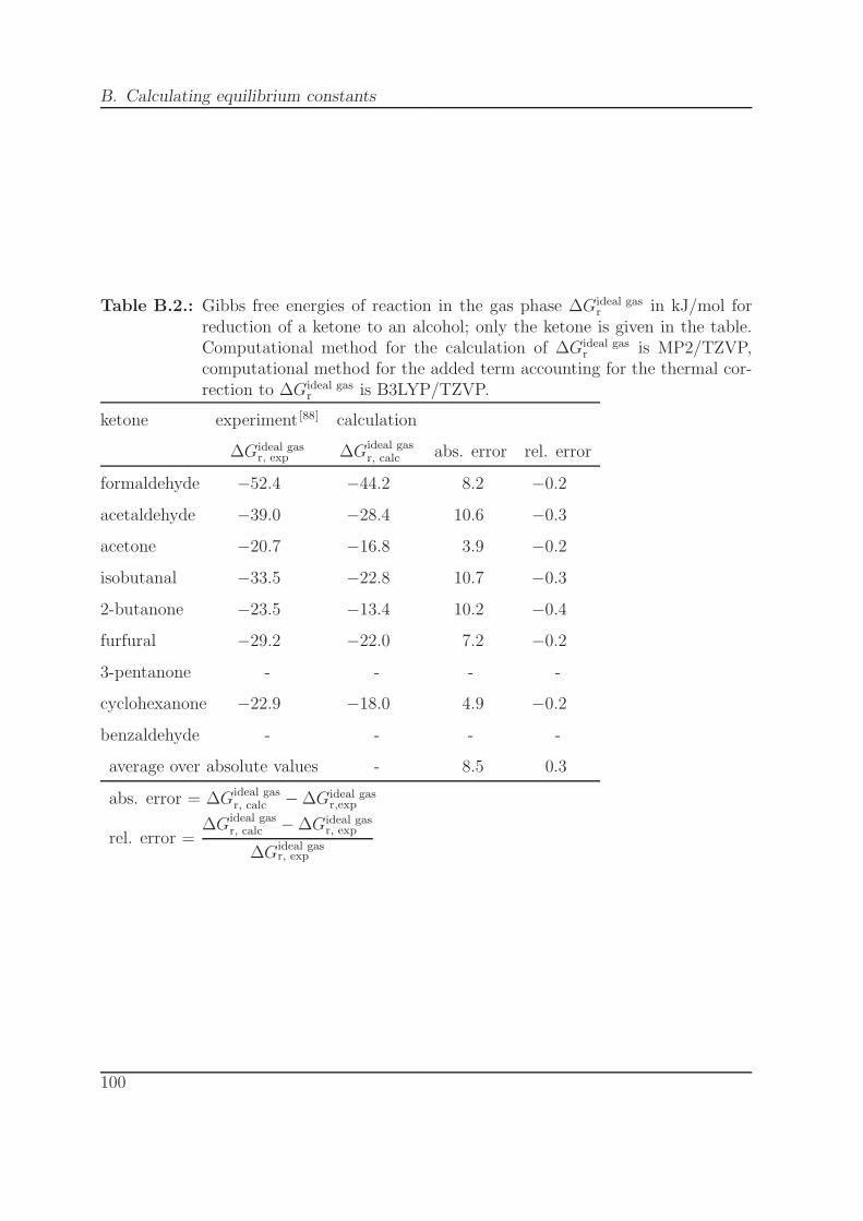
B. Calculating equilibrium constants
Table B.2.: Gibbs free energies of reaction in the gas phase ∆Gideal gasr in kJ/mol for
reduction of a ketone to an alcohol; only the ketone is given in the table.Computational method for the calculation of ∆Gideal gas
r is MP2/TZVP,computational method for the added term accounting for the thermal cor-rection to ∆Gideal gas
r is B3LYP/TZVP.
ketone experiment [88] calculation
∆Gideal gasr, exp ∆Gideal gas
r, calc abs. error rel. error
formaldehyde −52.4 −44.2 8.2 −0.2
acetaldehyde −39.0 −28.4 10.6 −0.3
acetone −20.7 −16.8 3.9 −0.2
isobutanal −33.5 −22.8 10.7 −0.3
2-butanone −23.5 −13.4 10.2 −0.4
furfural −29.2 −22.0 7.2 −0.2
3-pentanone - - - -
cyclohexanone −22.9 −18.0 4.9 −0.2
benzaldehyde - - - -
average over absolute values - 8.5 0.3
abs. error = ∆Gideal gasr, calc − ∆Gideal gas
r,exp
rel. error =∆Gideal gas
r, calc − ∆Gideal gasr, exp
∆Gideal gasr, exp
100
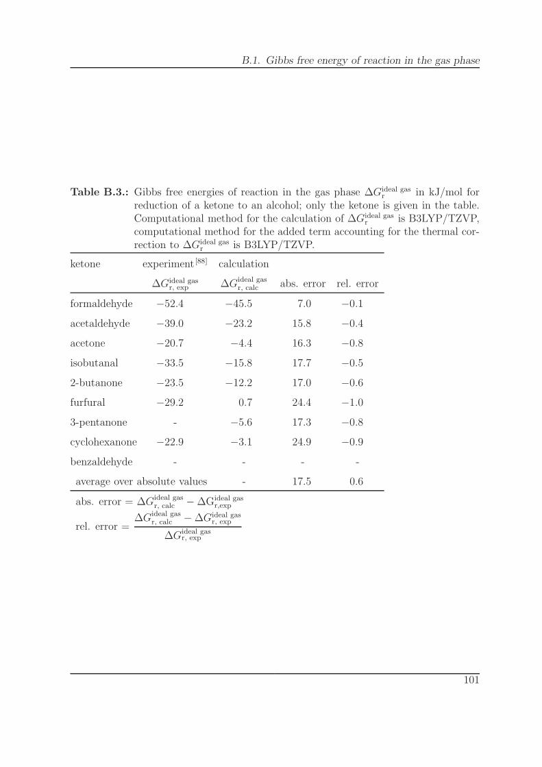
B.1. Gibbs free energy of reaction in the gas phase
Table B.3.: Gibbs free energies of reaction in the gas phase ∆Gideal gasr in kJ/mol for
reduction of a ketone to an alcohol; only the ketone is given in the table.Computational method for the calculation of ∆Gideal gas
r is B3LYP/TZVP,computational method for the added term accounting for the thermal cor-rection to ∆Gideal gas
r is B3LYP/TZVP.
ketone experiment [88] calculation
∆Gideal gasr, exp ∆Gideal gas
r, calc abs. error rel. error
formaldehyde −52.4 −45.5 7.0 −0.1
acetaldehyde −39.0 −23.2 15.8 −0.4
acetone −20.7 −4.4 16.3 −0.8
isobutanal −33.5 −15.8 17.7 −0.5
2-butanone −23.5 −12.2 17.0 −0.6
furfural −29.2 0.7 24.4 −1.0
3-pentanone - −5.6 17.3 −0.8
cyclohexanone −22.9 −3.1 24.9 −0.9
benzaldehyde - - - -
average over absolute values - 17.5 0.6
abs. error = ∆Gideal gasr, calc − ∆Gideal gas
r,exp
rel. error =∆Gideal gas
r, calc − ∆Gideal gasr, exp
∆Gideal gasr, exp
101
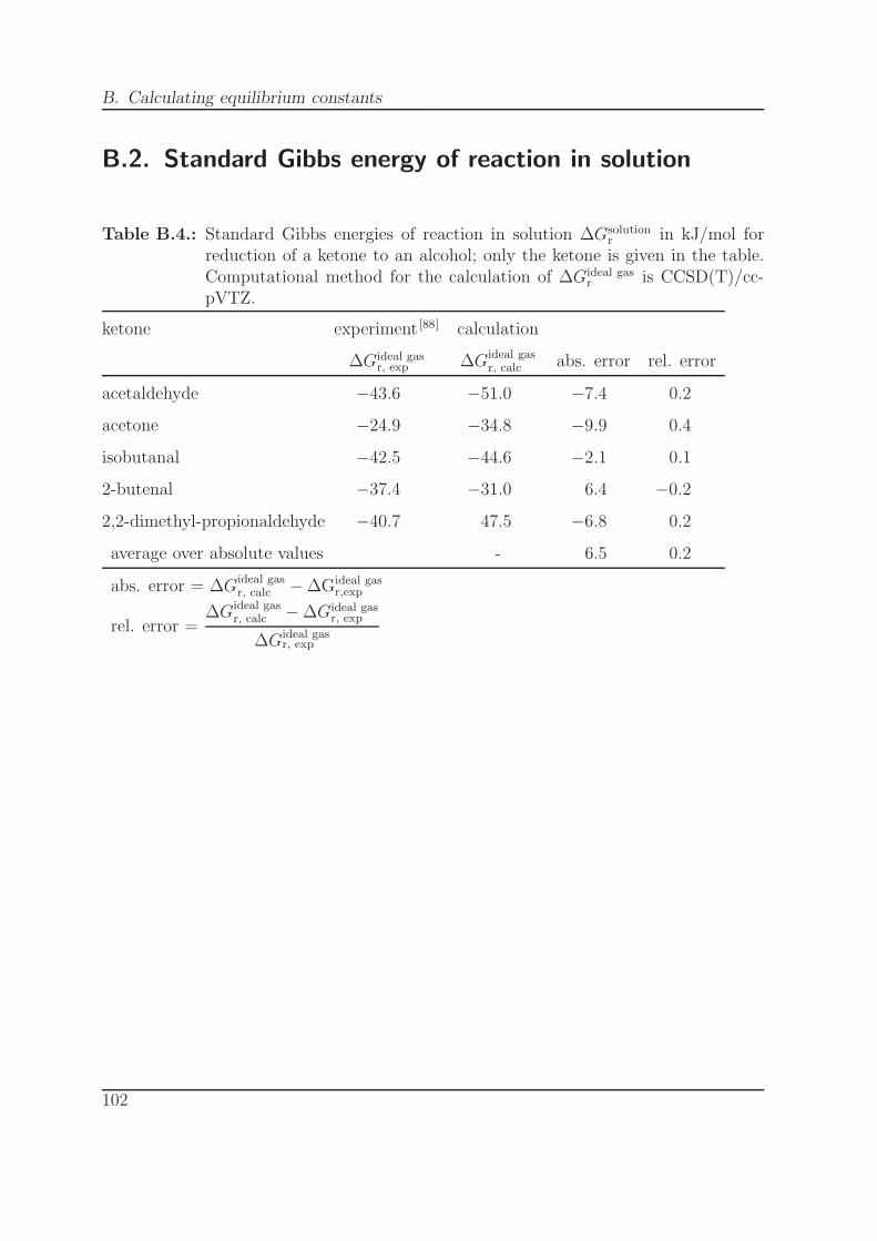
B. Calculating equilibrium constants
B.2. Standard Gibbs energy of reaction in solution
Table B.4.: Standard Gibbs energies of reaction in solution ∆Gsolutionr in kJ/mol for
reduction of a ketone to an alcohol; only the ketone is given in the table.Computational method for the calculation of ∆Gideal gas
r is CCSD(T)/cc-pVTZ.
ketone experiment [88] calculation
∆Gideal gasr, exp ∆Gideal gas
r, calc abs. error rel. error
acetaldehyde −43.6 −51.0 −7.4 0.2
acetone −24.9 −34.8 −9.9 0.4
isobutanal −42.5 −44.6 −2.1 0.1
2-butenal −37.4 −31.0 6.4 −0.2
2,2-dimethyl-propionaldehyde −40.7 47.5 −6.8 0.2
average over absolute values - 6.5 0.2
abs. error = ∆Gideal gasr, calc − ∆Gideal gas
r,exp
rel. error =∆Gideal gas
r, calc − ∆Gideal gasr, exp
∆Gideal gasr, exp
102

B.2. Standard Gibbs energy of reaction in solution
Table B.5.: Standard Gibbs energies of reaction in solution ∆Gsolutionr in kJ/mol for
reduction of a ketone to an alcohol; only the ketone is given in the table.Computational method for the calculation of ∆Gideal gas
r is MP2/TZVP.
ketone experiment [88] calculation
∆Gideal gasr, exp ∆Gideal gas
r, calc abs. error rel. error
formaldehyde −49.6 −63.4 −13.8 0.3
acetaldehyde −43.6 −45.1 −1.5 0.0
acetone −24.9 −31.4 −6.5 0.3
isobutanal −42.4 −39.0 3.5 −0.1
2-butenal −37.4 −26.2 11.3 −0.3
1-methoxy-2-propanone −36.5 −33.4 3.1 −0.1
2-butanone −23.7 −28.0 −4.3 0.2
cyclopentanone −23.8 −33.4 −9.7 0.4
2,2-dimethyl-propionaldehyde −40.7 −41.9 −1.2 0.0
furfural −41.2 −33.9 7.4 −0.2
1,3-dimethoxy-propan-2-one −67.5 −57.1 10.4 −0.1
2-methyl-2-butanone −23.7 −25.1 −1.4 0.1
cyclohex-2-enone −16.4 −14.2 2.2 −0.1
cyclohexanone −31.3 −32.1 −0.9 0.0
4-heptanone −19.5 −29.0 −9.5 0.5
4-methoxy-cyclohexanone −32.2 −20.6 11.6 −0.4
average over absolute values - 6.1 0.2
abs. error = ∆Gideal gasr, calc − ∆Gideal gas
r,exp
rel. error =∆Gideal gas
r, calc − ∆Gideal gasr, exp
∆Gideal gasr, exp
103
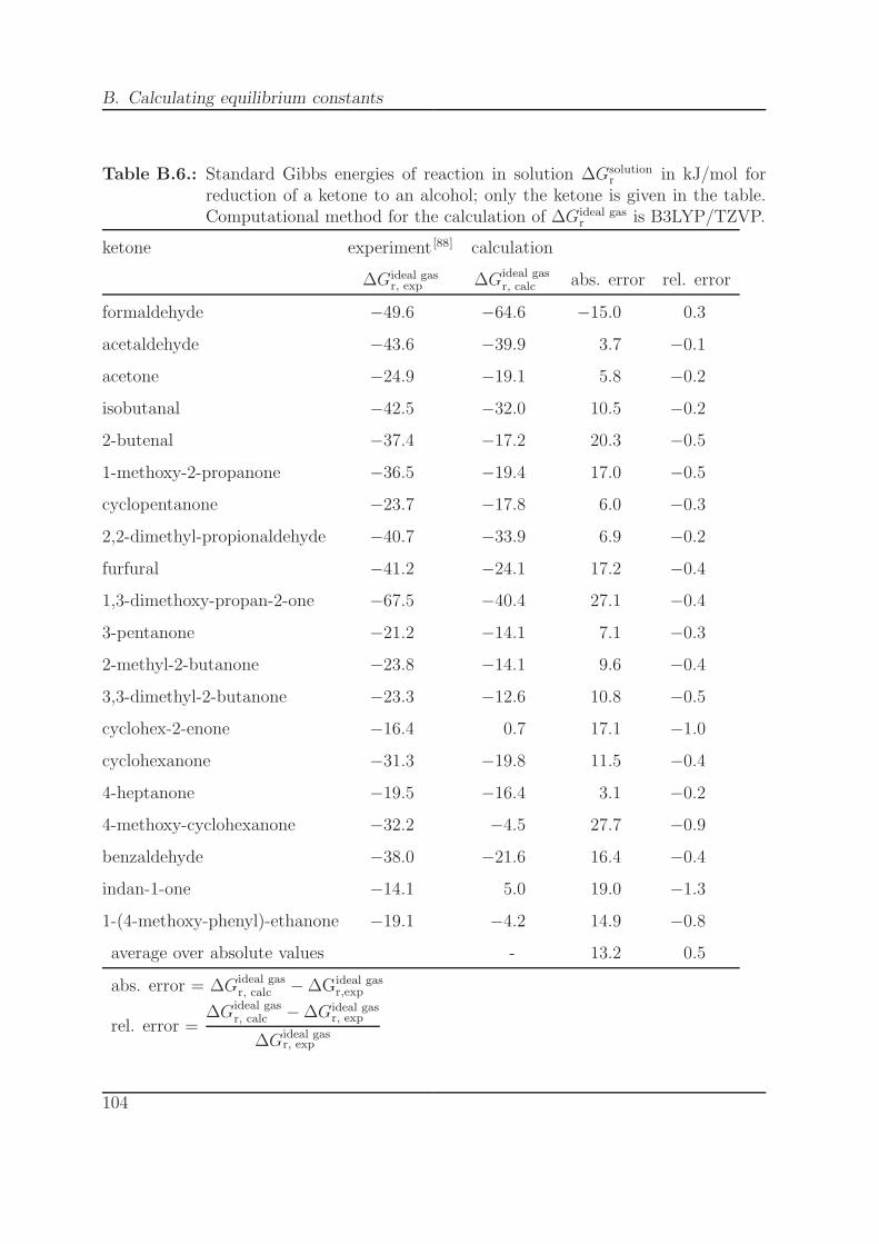
B. Calculating equilibrium constants
Table B.6.: Standard Gibbs energies of reaction in solution ∆Gsolutionr in kJ/mol for
reduction of a ketone to an alcohol; only the ketone is given in the table.Computational method for the calculation of ∆Gideal gas
r is B3LYP/TZVP.
ketone experiment [88] calculation
∆Gideal gasr, exp ∆Gideal gas
r, calc abs. error rel. error
formaldehyde −49.6 −64.6 −15.0 0.3
acetaldehyde −43.6 −39.9 3.7 −0.1
acetone −24.9 −19.1 5.8 −0.2
isobutanal −42.5 −32.0 10.5 −0.2
2-butenal −37.4 −17.2 20.3 −0.5
1-methoxy-2-propanone −36.5 −19.4 17.0 −0.5
cyclopentanone −23.7 −17.8 6.0 −0.3
2,2-dimethyl-propionaldehyde −40.7 −33.9 6.9 −0.2
furfural −41.2 −24.1 17.2 −0.4
1,3-dimethoxy-propan-2-one −67.5 −40.4 27.1 −0.4
3-pentanone −21.2 −14.1 7.1 −0.3
2-methyl-2-butanone −23.8 −14.1 9.6 −0.4
3,3-dimethyl-2-butanone −23.3 −12.6 10.8 −0.5
cyclohex-2-enone −16.4 0.7 17.1 −1.0
cyclohexanone −31.3 −19.8 11.5 −0.4
4-heptanone −19.5 −16.4 3.1 −0.2
4-methoxy-cyclohexanone −32.2 −4.5 27.7 −0.9
benzaldehyde −38.0 −21.6 16.4 −0.4
indan-1-one −14.1 5.0 19.0 −1.3
1-(4-methoxy-phenyl)-ethanone −19.1 −4.2 14.9 −0.8
average over absolute values - 13.2 0.5
abs. error = ∆Gideal gasr, calc − ∆Gideal gas
r,exp
rel. error =∆Gideal gas
r, calc − ∆Gideal gasr, exp
∆Gideal gasr, exp
104
C. Acknowledgements
Leider laßt sich eine wahrhafte Dankbarkeit
mit Worten nicht ausdrucken.
Johann Wolfgang von Goethe (1749-1832)
Special thanks go to ...
... Prof. Dr. Walter Leitner for supervision, expert knowledge and expertise, indepen-
dence, career advancement, good advice
... Prof. Dr.-Ing. Andreas Pfennig for expert knowledge, straightforward interdisci-
plinary discussions, critical remarks and suggestions, an engineering point of view
... Prof. Dr. Marcel Liauw for inspiring, motivating and worthwhile discussions, Dutch
training, good advice
... Dr. Lasse Greiner for supervision, trust, the positive and enjoyable office atmosphere,
Dilbert, and for all straightforward discussions about chemistry and beyond
... Dr.-Ing. Antje Spieß for supervision, trust, the engineering way, exchange of experi-
ence, pleasant conversations with a cup of tea
... Dr. Kai Leonhard for help, support, patience, expert knowledge
... Dipl.-Ing. Michael Zavrel, Dr. Marrit Eckstein and Dr. Markus Hoelscher for valuable
cooperations, interdisciplinary discussions, important critical remarks
... Dr. Marrit Eckstein, Dipl.-Ing. Michael Zavrel, Dr. Werner Eberhard, Dipl.-Chem.
Julia Lembrecht and Dr.-Ing. Thomas Schmidt for generous supply of experimental
data
105

... Dipl.-Ing. Michael Zavrel, Dr. Kai Leonhard, Dr.-Ing. Antje Spieß, Dipl.-Chem.
Clemens Minnich, Dipl.-Chem. Marc Lecour, Dr. Marrit Eckstein, Dr. Lasse Greiner
and Dr. Morgan Thomas for proof reading
... Dr. Andreas Klamt, Dr. Michael Diedenhofen and Dr. Frank Eckert for Turbomole
and COSMOtherm support
... DFG graduate school 1166 BioNoCo (Biocatalysis using non-conventional media) for
financial support and numerous possibilities for further education
... all scientific and non-scientific colleagues at the Institute of Technical and Macromolec-
ular Chemistry for cooperativeness, discussions, enjoyable working atmosphere and many
broad laughters
... my family, friends and especially my parents and Johannes for support, patience and
understanding
106
D. Curriculum vitae
PERSONAL
Name Martina Peters
Date of birth January 14, 1980
Place of birth Bitburg, Germany
Nationality German
EDUCATION
04/2007 - 07/2007 Research stay, Shell Global Solutions, Amsterdam, The
Netherlands, Prof. ir. Jan Harmsen
12/2005 - 12/2008 Doctoral thesis, Institute of Technical and Macromolecular
Chemistry, RWTH Aachen University, Germany, Prof. Dr.
Walter Leitner
05/2005 - 10/2005 Diploma thesis, Institute of Technical and Macromolecular
Chemistry, RWTH Aachen University, Germany, Prof. Dr.
Walter Leitner
04/2000 - 10/2005 Chemistry studies, RWTH Aachen University, Germany and
University of Colorado at Boulder, USA
10/1999 - 09/2000 Biology studies, RWTH Aachen University, Germany
09/1992 - 06/1999 Secondary school, St.-Willibrord Gymnasium, Bitburg, Germany
107
Top Related