


Languages
Pages
Legal


Monetary Transmission
via the Administered Interest Rates Channel
By
Beng-Soon Chong
Nanyang Business School, NTU, Singapore
Ming-Hua Liu*
Faculty of Business Auckland University of Technology, New Zealand
Keshab Shrestha
Nanyang Business School, NTU, Singapore
Abstract
This paper examines the dynamics of administered interest rate changes in response to changes in the benchmark money market rate in Singapore. Our results show that the administered rates’ adjustment speed differs across both financial institutions and financial products. The financial institutions’ administered (lending and deposit) rates, moreover, are more rigid when they are below their equilibrium level than when they are above. Our finding, hence, implies that the speed of monetary transmission is not uniform across all sectors of the economy and that a tightening monetary policy takes a longer time to impact the economy than an expansionary monetary policy.
JEL classification: E43 Key Words: Monetary Policy, Transmission Mechanism, Interest Rates,
Asymmetric Adjustment, Price Rigidity
Correspondence may be sent to: Ming-Hua Liu, email: [email protected]
Monetary Transmission
via the Administered Interest Rates Channel
Abstract
This paper examines the dynamics of administered interest rate changes in response to changes in the benchmark money market rate in Singapore. Our results show that the administered rates’ adjustment speed differs across both financial institutions and financial products. The financial institutions’ administered (lending and deposit) rates, moreover, are more rigid when they are below their equilibrium level than when they are above. Our finding, hence, implies that the speed of monetary transmission is not uniform across all sectors of the economy and that a tightening monetary policy takes a longer time to impact the economy than an expansionary monetary policy.
1. Introduction
In this paper, we examine the dynamics of administered interest rate changes in response
to changes in the benchmark market rates across different financial institutions (namely,
commercial banks and finance companies) and across different financial products
(namely, saving deposits, time deposits with various maturities, hire-purchase loans,
mortgages, and commercial loans).
1

At the micro-level, such a study can provide us with a better understanding of the
administered rate-setting behavior of different financial institutions. Banks have a
significant amount of products with embedded options such as the early withdrawal of
deposits and prepayment of loans (including mortgages, overdraft, and credit card loans).
To value and risk-manage such products, option-adjusted spread (OAS) analysis is
typically carried out. Modeling the relationship between the interbank rate and
administered (deposit and loan) rates is an essential part of the OAS analysis. Hence, our
study has significant implications for the valuation and risk management of option-
embedded banking products such as current account deposits, savings deposits,
mortgages, mortgage-backed securities, credit-card receivables, etc.
At the macro-level, an important question in the conduct of monetary policy is how fast
financial institutions pass through changes in the market intervention rates to their
customers. The existence of differential adjustment rates across financial institutions and
across financial products, if any, has important implications for the conduct of monetary
policy as it implies that the speed of monetary transmission is not uniform across
different segments of the banking sector. Further, the adjustment speed can be different
depending on whether rates are above or below their long-term equilibrium level. It is
well known that monetary policy operates with lags, partly due to the delay by financial
institutions in adjusting their administered rates when market rates change. By examining
the different adjustment speed of various financial institutions/products and the
asymmetric nature of the adjustment speed, our study can shed additional light on how
monetary policy is transmitted via changes in financial institutions’ administered rates.
2
There are two possible approaches to study the role of depository institutions in the
monetary transmission mechanism. One approach is to examine how monetary policy is
transmitted through the bank lending channel. Previous studies on bank lending channel
typically analyze how the banks’ balance sheet items respond to changes in monetary
policy stance, which is usually proxied by changes in the interbank rate. For example, in
the event of a liquidity squeeze, some banks may respond by raising new deposits to
maintain or even increase their lending level. Others may use their excess capital to
maintain their loan supply. Evidence on bank lending channel in the United States shows
that monetary policy is transmitted mainly through small banks that are either illiquid or
undercapitalized (Kashyap and Stein, 2000; Kishan and Opiela, 2000). Evidence in
Europe is rather mixed, i.e. banks in different countries appear to respond differently to
protect their loan supply from changes in monetary policy. Altunbas et al. (2002) finds
that monetary policy is transmitted mainly through undercapitalized banks in smaller
EMU countries, while Kakes and Sturm (2002) find that monetary policy in Germany is
transmitted mostly through small banks.
Another approach, which is undertaken in this study, is to examine how monetary policy
is transmitted through the administered rates channel. The relationship between the
market rate and the administered rates is a complicated one and the evidence presented,
thus far, is mixed and inconclusive. Hannan and Berger (1991), for example, examine the
deposit rate setting behavior of commercial banks in the United States and find that: (a)
firms in more concentrated market exhibit greater price rigidity; (b) larger firms exhibit
less price rigidity; and (c) deposit rates are more rigid upwards than downwards.
3
Scholnick (1996), similarly, finds that deposit rates are more rigid when they are below
their equilibrium level than when they are above. His finding on lending rate adjustment,
however, is mixed. Heffernan (1997) examines how the lending and deposit rates of four
banks and three building societies respond to changes in the base rate set by the Bank of
England and finds that (a) there is very little evidence on the asymmetric adjustments in
both the deposit and lending rates, (b) there is no systematic difference in the
administered rate pricing dynamics of banks and building societies, and (c) the
adjustment speed for deposit rates is, on average, roughly the same as that for loan rates.1
Our finding, in contrast, shows that the adjustment speed of administered rates in
response to changes in the benchmark market rate varies across both financial institutions
and financial products and tends to be asymmetric. More specifically, our paper yields
three key results. First, we find that the administered rates’ adjustment speed differs
across financial institutions. Finance companies’ deposit rates, in particular, are less rigid
than those of commercial banks, but their loan rates are generally more rigid. Second,
our result shows that the adjustment speed differs across financial products. Loan rates, in
particular, tend to adjust more slowly than deposit rates. Third, we find that both the
lending and deposit rates are more rigid when they are below their equilibrium level than
when they are above. Our overall finding, hence, implies that the speed of monetary
transmission is not uniform across all sectors of the economy and that a tightening
monetary policy takes a longer time to impact the economy than an expansionary
monetary policy.
1 Heffernan (1997), however, finds a wide variation in the adjustment speed within each type of financial institutions and products.
4
We, in addition, find that it is not true in general that monetary policy is transmitted
mostly through the smaller financial institutions (as is found in the literature on bank
lending channel). Our results suggest that financial institutions have the choice of
responding via the administered rates channel and/or the bank lending channel. In the
loan market, the larger financial institutions (commercial banks) are more likely to
respond to a change in monetary policy via the administered rates channel, while the
smaller financial institutions (finance companies) are more likely to respond via the bank
lending channel.
The remainder of the paper is organized as follows: Section 2 provides some institutional
background about Singapore’s depository financial institutions. Section 3 examines the
conceptual framework for asymmetric price rigidity. Section 4 outlines our methodology.
Section 5 discusses the results and the final section concludes the paper.
2. Institutional Background
In this paper, we examine the administered rates setting behavior of two types of
depository financial institutions in Singapore, namely the commercial banks and finance
companies.2 Commercial banks are the single most important financial institutions in
Singapore. They can be further classified into three subgroups based on the type of
licence held: full licensed banks, wholesale banks, and offshore banks. Full licensed
banks may engage in all types of banking activities. As at March 2002, six of the 22 full
5

licensed banks are locally-incorporated under the umbrella of three domestic banking
groups (DBS, UOB, and OCBC). The other full licensed banks are branches of foreign-
incorporated banks. Although small in numbers, the domestic banks are very important
players in the domestic banking market, controlling over 90% of total deposits from non-
bank customers in Singapore (Luckett et al., 1994). As at March 2002, there are 33
wholesale banks and 59 offshore banks, all of which are branches of foreign banks.
Wholesale banks’ activities are somewhat restricted as they are not allowed to engage in
Singapore Dollar retail banking activities. The offshore banks, moreover, are mostly
restricted to the offshore (international) banking activities.
Finance companies in Singapore undertake small-scale financing, which includes hired-
purchase financing and mortgage loans for housing. They play an important role in the
financial system by lending mostly to individuals and small businesses. Table 1 provides
a comparison of the asset & liability structure of the commercial banks and finance
companies in Singapore. In terms of size, the finance companies are much smaller than
the commercial banks. Their major sources of funds are deposits from individuals and
institutions, which account for more than 70% of total funding. In contrast, total deposits
accounts for only 51% of commercial banks’ total funding as at end-2002. Finance
companies, moreover, are not allowed to accept demand deposits. The finance
companies’ major uses of funds are loans, which account for 79% of their total assets as
at end-2002. They also place deposits with banks and other institutions. Finance
companies are not allowed to make unsecured loans exceeding S$5,000 to any persons or
2 Merchant banks in Singapore are non-depository financial institutions and, hence, are excluded in this study. There is, furthermore, no available interest rate data on merchant banks.
6
to deal in foreign currencies, gold or other precious metals or to acquire foreign currency
denominated stocks or bonds. The commercial banks, in contrast, have a more diversified
portfolio of assets. For example, the banks’ total loans, which accounts for only 46% of
their total assets, are generally more diversified across different sectors of the economy.
The finance companies are nevertheless important players in the financial sector and their
role in the financial intermediation process remains significant despite increasing
competition from both the commercial banks and non-banking institutions recently.
_______________________________________
INSERT TABLE 1 HERE
_______________________________________
3. Conceptual Framework for Asymmetric Price Rigidities
Evidence of price rigidity has been well documented for a variety of industries in the
developed countries. Among the earlier studies, Mills (1927), for example, used the
Bureau of Labor Statistics data on prices collected for the construction of consumer price
index (CPI) in the USA to examine the rigidities in wholesale prices for a whole range of
goods. More recently, Cecchetti (1986) provides evidence on the rigidities in newsstand
prices for magazines. Carlton (1986) examines the rigidities in the prices of industrial
commodities and concludes that there are significant price rigidities in a number of
industries, including the steel, chemical and cement industries. Kashyap (1995) similarly
provides evidence of rigidities in the prices of retail catalogs. Peltzman (2000), moreover,
7

finds in a more comprehensive study of 77 consumer and 165 producer goods that the
odds are better than two to one that output prices tend to react faster to input price
increases than decreases. Hannan and Berger (1991), Scholnick (1996), and Heffernan
(1997), furthermore, provide evidence on the rigidities in the deposit rate and loan rate
adjustments in the banking industry.
The rigidity in price adjustment may be due to several factors, namely: fixed menu cost,
high switching cost, imperfect competition, and asymmetric information. Under the
traditional menu costs hypothesis in economics, firms are reluctant to re-quote the prices
of their products if changes in those prices are deemed to be very small (in comparison to
the advertisement and promotional costs associated with re-pricing the products) and/or
temporary in nature. Instead, firms tend to adjust their prices less frequently and by a
larger amount when prices move away from the equilibrium level. The expected price
rigidity under the menu costs hypothesis, however, is symmetric.3
Price rigidity is also affected by the existence of high switching costs. According to
Heffernan (1997), uninformed customers are less likely to switch financial products
and/or institutions in search of the best price or yield when there are (perceived or real)
high switching costs.4 The rigidity in prices, therefore, may be attributed to the banks’
exploitation of consumers’ inertia in switching financial products and/or institutions.
Heffernan (1993), for example, provides evidence on banks’ sophisticated price
3 For more information on menu costs hypothesis and its economic implications, refer to Blinder (1994), Duta et al. (1999), and Mankiw (1985). 4 Switching costs, in particular, tend to be high in market segments that require long-term relationship building and repeated transactions.
8

discrimination practices where the rates on certain banking products were initially offered
at bargain or competitive level, but allowed to grow less competitive over time. If banks
can price-discriminate to exploit customers’ inertia, then rates are expected to be rigid
upwards for customer deposits, but rigid downwards for loans.
Rigidities in interest rate adjustments can also be attributed to imperfect competition in
the market (Hannan and Berger, 1991). Administered rates, for example, are likely to
adjust more slowly in an uncompetitive market. Moreover, because of the collusive price
arrangement among banks, rate adjustments in uncompetitive markets can be asymmetric.
For example, in the presence of collusive pricing behavior, deposit rates are expected to
be rigid upwards, while loan rates are expected to be rigid downwards.
Finally, loan rate adjustment can be sluggish due to the existence of asymmetric
information. In Stiglitz and Weiss (1981) model, banks encounter both adverse selection
and moral hazard problems when they are required to raise loan rates in response to rising
wholesale market interest rates. Adverse selection problem arises because higher loan
rates are more likely to attract clienteles that are of higher risk. Moral hazard problem
arises because higher loan rates may increase existing borrowers’ incentives to undertake
high risks and high expected returns projects, in order to compensate for the higher
borrowing cost. Increases in loan rates, therefore, may result in greater likelihood of
default among existing borrowers. In view of these problems, banks are generally
reluctant to raise loan rates significantly over a short period of time. Instead, the banks
are more likely to ration the amount of credit extended when there is an upward pressure
9
on loan rates. Loan rates, consequently, are expected to be more rigid upwards under
Stiglitz and Weiss (1981) asymmetric information model.
Hence, given the above hypotheses, it is an empirical question as to whether the deposit
rates and loan rates are more rigid upwards or downwards. A summary of the predicted
price rigidities under the various hypotheses is given in Table 2 below. 5
_______________________________________
INSERT TABLE 2 HERE
_______________________________________
According to the above hypotheses, it is likely that the rigidity in administered rates vary
across different financial institutions and across different products. Variation in the price
rigidities of different financial products is possible if financial institutions can selectively
price-discriminate on certain products, depending on the relative level of customers’
inertia or switching costs. Customer inertia for saving deposit, for example, may be
greater than for time deposits. Price rigidities, therefore, are likely to be greater for
5 Administered price rigidities in certain countries may be attributed to the direct and/or indirect government interventions. As a matter of national policies, governments in certain countries often protect their financial institutions by encouraging downward rigidities in loan rates and/or upward rigidities in deposit rates. Direct government interventions, for example, may be in the form of interest rates regulations, while indirect intervention may be in the form of regulatory moral suasions. At the same time, it is also not unusual for government in certain countries to intervene on behalf of borrowers by encouraging upward rigidity in loan rates or on behalf of consumers by encouraging downward rigidities in deposit rates. Hence, although price rigidities in certain countries may be attributed to government interventions, the expected direction of price rigidities is mixed i.e. depending on the relative political and economic influences of various special-interest groups (financial institutions, borrowers, or consumers). In Singapore, rate setting is seen as the operational decisions of financial institutions and the authority does not regulate both the deposit and lending rates.
10
products with greater customer inertia. As a result, such financial products will be less
responsive to changes in market conditions.
Variation in price rigidities across different financial institutions is also likely if there are
significant differences in the price setting behavior of financial institutions. In setting
administered prices, some financial institutions may be price leaders, while others may be
price followers. In such a price leader-follower paradigm, prices are anticipated to be
more rigid for institutions that are of the price-followers type. Rigidities in prices across
different institutions, furthermore, may be attributed to the relative inertia of customers,
which form the institutions’ client base. Institutions that have a higher percentage of inert
customers, hence, are more likely to exhibit greater rigidities in administered prices.
Different factors, moreover, are likely to play a different role in the administered rates’
(short-term and long-term) adjustment process. Switching cost and menu costs, for
example, are more likely to be the primary factors in influencing the short-term
adjustment speed whereas imperfect competition and asymmetric information are more
likely to be the primary factors in affecting the long-term adjustment process.
4. Methodology
In this paper, we examine both the long-run and short-run dynamics of administered rate
changes. First, the long-term relationship between the administered rate and the market
rate is as follows:
ttt xy εαα ++= 10 (1)
11

where represents the endogenous administered (lending or deposit) rates; denotes
the corresponding interbank rate (which is assumed to be exogenous);
ty tx
tε is the
disturbance term; 0α and 1α are the model parameters. As discussed in Rousseas
(1985), 0α measures the constant markup and 1α measures the degree of pass-through in
the long term. The long-run adjustment is complete when 1α is equal to one. It is,
however, incomplete ( 1α is less than one) when markets are not fully competitive and
when there are high switching and menu costs and/or asymmetric information.
Second, to examine the short-run dynamics of administered rate changes in response to
changes in the market rate, we employed an error-correction methodology that is
similarly used in Heffernan (1997) and Scholnick (1996). Using the error-correction
model, we can test for differences in the administered rate adjustments when they are
above or below their equilibrium level.6 Finally, the error-correction model also allows
us to determine how long it takes for the administered rates to fully adjust to changes in
wholesale rates in the market.
Given that most time series data are non-stationary in nature (Granger and Newbold,
1986), the Engle-Granger (1987) cointegration and error-correction procedures can be
applied to remove any spurious results. If the two series, yt and xt, are found to be
integrated of order one, I(1), and their linear combination is found to be stationary
6 Hannan and Berger (1991), in contrast, used the multinomial logit model to test for asymmetric rigidities in deposit rates.
12

(integrated or order zero, I(0)), then they are said to be cointegrated. In this case, the
following error-correction representation exists:
ttttt xyxy νααββ +−−+∆=∆ −− )( 110121 (2)
where denotes first difference; ∆ 1β measures the short-term pass-through rate, and tν is
the error term. ( 1011ˆ
−−− −− )1= ttt y xααε , which represents the extent of disequilibrium at
time ( , is the residual of the long run relationship given by equation (1). β)1−t 2, hence,
captures the error correction adjustment speed when the rates are away from their
equilibrium level. In the mean reverting case, the sign of 2β is expected to be negative.
Following Hendry (1995), the mean adjustment lag of a complete pass-through can be
calculated as follows:
21 /)1( ββ−=MAL (3)
But, in order to incorporate the possibility of asymmetric adjustments in the administered
rates when they are above or below their equilibrium levels, we use an indicator
variable,λ . The indicator variable (λ ) is equal to one if the residual error
( 1101ˆ
−− −−= tt xy 1−t ααε ) is positive and 0 otherwise. The asymmetric short-run dynamic
equations can, therefore, be written as:
∆ (4) ttttt xy ηελδελδδ +−++∆= −− 13121 ˆ)1(ˆ
where 2δ captures the error correction adjustment speed when the rates are above their
equilibrium values and 3δ captures the error correction adjustment speed when the rates
are below their equilibrium values. To detect the presence of asymmetric adjustment, we
use the standard Wald test to determine if 2δ is significantly different from 3δ .
13
As with the symmetric adjustment case, we can define the asymmetric mean adjustment
lags of a complete pass-through as follows:
21 /)1( δδ−=+ML (5)
31 /)1( δδ−=−ML (6)
where +ML represents mean adjustment lag when the administered rates are above their
equilibrium value and −ML represents the mean adjustment lag when the administered
rates are below their equilibrium value
5. Data and Analysis of Results
The monthly series of interest rate data for both the banks and finance companies in
Singapore were taken from the Monthly Statistical Bulletin, which is regularly published
by the Monetary Authority of Singapore (MAS), the de facto central bank of Singapore.7
The sampling period, which is from January 1983 to December 2002, covers a time span
of 20 years. The sample size is, therefore, 240 for each interest rate series.
In our study, the changes in monetary policy stance are proxied by the changes in the
benchmark 3-month Singapore interbank offered rate (SIBOR) in the money market. As
the de-facto central bank in Singapore, the Monetary Authority of Singapore (MAS)
influences interest rate indirectly. As Singapore is a small and open economy, the
government adopts a managed float exchange rate regime on a trade-weighted basis. The
7 The data are freely available from the MAS website: www.mas.gov.sg.
14

MAS intervenes in the money market in order to maintain the band it has established for
the Singapore dollar against the trade-weighted basket of currencies. Any changes in the
domestic money market rates, hence, affect both the country’s exchange rate and the
financial institutions’ deposit and loan rates.
For commercial banks, the benchmark lending rate is the prime rate (PRIME) and the
referenced deposit rates are: the savings deposit rate (BSaving), the 3-month fixed
deposit rate (BFD3), the 6-month fixed deposit rate (BFD6) and the 12-month fixed
deposit rate (BFD12). For finance companies, the referenced administered rates are: the
15-year housing loan (HL), the 3-year hire purchase loans on new vehicle (HP), the
savings deposit rate (FSaving), the 3-month fixed deposit rate (FFD3), the 6-month fixed
deposit rate (FFD6) and the 12-month fixed deposit rate (FFD12).
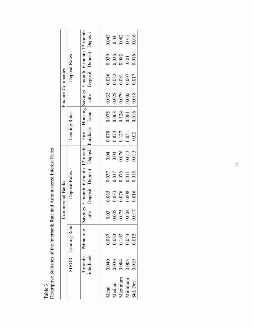
Table 3 provides the descriptive statistics for the sample data. The deposit rates for both
the banks and finance companies are positively related with maturity, indicating an
upward sloping yield curve. Finance companies, moreover, tend to offer higher deposit
rates than commercial banks. This is consistent with the fact that finance companies tend
to rely more heavily on deposits as a source of funding and that finance companies have
higher default risk than banks. As there is no deposit insurance scheme in Singapore,
finance companies, which are much smaller than banks, have to pay a premium in order
to attract deposits. The banks’ and finance companies’ lending rates are not comparable
as they are a function of credit risk as well as funding costs.
15

_______________________________________
INSERT TABLE 3 HERE
_______________________________________
Table 4 shows the correlation coefficient among the variables. Correlation analysis yields
three interesting results. First, in comparison to the loan rates, the deposit rates are, on
average, more highly correlated with the SIBOR. Second, the correlation between the
SIBOR and deposit rates tends to increase with the maturity of the deposit rates. Third, in
comparison to the commercial banks, the finance companies’ deposit rates are more
highly correlated with the SIBOR, but their loan rates are less correlated with the SIBOR.
_______________________________________
INSERT TABLE 4 HERE
_______________________________________
In order to determine the dynamics of administered rate changes in response to changes
in the benchmark market rate (SIBOR), we first carry out the Granger causality test to
determine if changes in the SIBOR cause adjustments in the administered interest rates.
Table 5 reports the results of the Granger causality test. As expected, changes in the
SIBOR cause all the administered rates to change.
_______________________________________
INSERT TABLE 5 HERE
_______________________________________
16
Having determined the dependent and independent variables, we then carry out
stationarity and cointegration tests to examine whether the various administered interest
rates (lending rate and deposit rate) are cointegrated with the benchmark market rate
(SIBOR). If the administered rates are cointegrated with the benchmark market rate, then
there is a long-term relationship between the administered rates and the benchmark
market rate. In other words, the administered rates are adjusted in response to changes in
the benchmark market rate.
Prior to the cointegration tests, however, we must first establish the non-stationarity of
the level of interest rate series and the stationarity of the first-differenced interest rate
series. Both the Augmented Dickey Fuller (ADF) and Philips Perron (PP) procedures test
the null hypothesis of unit root against the alternative hypothesis of stationarity.
However, such unit-root tests tend to have low power in distinguishing between the null
and the alternative (DeJong et al., 1992). As a consequence, we can also apply the KPSS
procedure to test the null hypothesis that the interest rate series are stationary
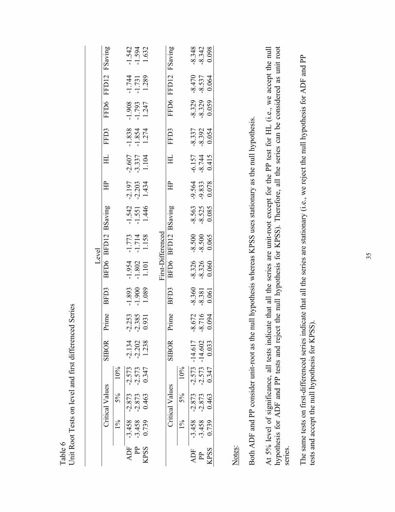
(Kwiatkowski et al., 1992). The results of the stationarity tests on the various interest
rate series are summarized in Table 6. For the level of the series, the above three
stationarity tests conclusively show that, at 5% level of significance, all the series are unit
root non-stationary.8 The results summarized in Table 6 also show that all the first
differenced series are stationary. This implies that all the series have single unit-root.
This is exactly the condition necessary for performing the cointegration tests.
8 An exception is in the case of the finance companies’ housing loan rate (HL) where the results are less conclusive because the non-stationarity of the level of the interest rate series is supported by both the ADF and KPSS tests, but not the PP test.
17
_______________________________________
INSERT TABLE 6 HERE
_______________________________________
The results of the cointegration tests are reported in Table 7. The ADF test results show
that all the administered rates are cointegrated with the SIBOR at 10% significance level,
except for the finance companies’ hire purchase and housing loan rates. To test for
robustness, we also run the Johansen’s Trace and Lambda-Max tests, which are
considered to be more powerful than the ADF test.9 The results of the Johansen tests
show that that all the administered rates are cointegrated with the SIBOR.
_______________________________________
INSERT TABLE 7 HERE
_______________________________________
The cointegration test results, hence, show that there is a statistically significant long-
term relationship between the benchmark market rate (SIBOR) and the administered
interest rates of both the commercial banks and the finance companies. The estimated
coefficients of the long-term relationship (Equation 1) are reported in Table 8.
_______________________________________
INSERT TABLE 8 HERE
_______________________________________
9 Johansen’s tests are considered to be more powerful than the Engle-Granger’s ADF test since they do not require an arbitrary assignment of one of the series to be left-hand side series.
18

The intercept of Equation 1 measures the markup whereas the slope measures the long-
term rate of pass-through. As expected, the markup for loan rates is much higher than that
of deposit rates. On average, the markup for loan rate is about 5% whereas for deposit
rates, it is about less than 1%. As for the degree of pass-through, our results show that
the pass-through for both the loans rates and deposit rates are not complete.10 In the case
of loan rates, it is about 50% (except for HP which is about 80%). The reason for the
relatively higher pass-through rate on the hire-purchase loans is probably that the hire-
purchase market is generally more competitive than the other loan markets as hire-
purchase credits are also provided by non-financial institutions (such as the participating
merchants themselves).
For deposit rates, their pass-through rate (which is in the range of 70% to 80%) is, on
average, higher than that of the loan rates.11 This is probably due to higher switching
costs in the loan market as compared to the deposit market. As a result, it is easier for
customer to switch banks when deposit rates are not competitive than when loan rates are
not competitive. The relatively lower degree of pass-through for the loan rates, moreover,
may be due to adverse selection and moral hazard reasons cited in the Stiglitz-Weiss
(1981) asymmetric information model.
10 The degree of the long-term pass-through is determined by the demand elasticity of deposits and loans to bank administered rates. It is less than one if the demand for loans or deposits is not fully elastic. The degree of the long-term pass-through is also influenced by the degree of market power. Rates in uncompetitive segments of the market adjust incompletely, resulting in a degree of pass-through that is less than one. 11 The difference in the pass-through rate for the deposit rates and the loan rates is found to be statistically significant using the Wald test. The detailed results of the Wald tests are available from the authors upon request.
19
The long-term adjustment results also show that the pass-through rate on finance
companies’ deposit rates is statistically higher than that of the commercial banks.12 For
example, the pass-through rate on finance companies’ and banks’ saving deposits are,
respectively, 84% and 75%. The average pass-through rate on finance companies’ and
banks’ fixed deposits are, respectively, 79% and 72%. This result may be attributed to
the fact that finance companies (in comparison to commercial banks) are smaller and
riskier and tend to rely more on deposits as a primary source of funding. The finance
companies, hence, are required to compete more aggressively for deposits by not only
offering higher deposit rates, but also re-adjusting their rates more frequently to changes
in the market rates.
Among the deposit rates, the pass-through rate on the finance companies’ savings deposit
rates is statistically higher than that of its fixed deposit rates. This result may be attributed
to competitive reasons where financial institutions tend to compete more for savings
deposit, which is less costly and considered as core deposit, than for fixed deposits. We,
however, do not find any statistical difference in the pass-through rates among the
finance companies’ fixed deposit rates of various maturities as well as among the banks’
fixed deposit rates.13
As the administered rates are found to be cointegrated with the benchmark market rate
(SIBOR), the proper short-run dynamics is given by the error-correction model. The
results of the symmetric ECM (Equation 2) are reported in Table 9. As expected, all the
12 The detailed results of the statistical tests are available from the authors upon request. 13 The detailed results of the (Wald) statistical tests are available from the authors upon request.
20

estimates of 2β are found to be negative and statistically significant. The results show
that the administered rates are mean-reverting to long-run equilibrium. In other words,
the rates will adjust upwards when they are below the equilibrium level and adjust
downwards when the rates are above their equilibrium levels.
_______________________________________
INSERT TABLE 9 HERE
_______________________________________
It is widely known that market interest rates follow a mean-reverting process, but the
short-term adjustment speed is not necessarily the same when the rates are above their
equilibrium level as when they are below. The results for the asymmetric ECM (Equation
4) are reported in Table 10. Comparing δ2 and δ3, we find that both the banks and
finance companies adjust their deposit and loan rates downwards faster than they adjust
them upwards. The difference, as indicated by the Wald test, is statistically significant for
all the administered rates, with the exception for the 12-month fixed deposit rates and
hire-purchase loan rates (HP).
_______________________________________
INSERT TABLE 10 HERE
_______________________________________
The issue of different adjustment speed is further examined with the estimation of mean
adjustment lags (MAL) for both the symmetric and the asymmetric models. The mean
21
adjustment lags of the commercial banks’ and finance companies’ administered rates are
reported in Table 11.
_______________________________________
INSERT TABLE 11 HERE
_______________________________________
The results in Table 11 show that the short-run adjustment speed differs across financial
products as well as across financial institutions. For example, we find that the short-run
adjustment speed for the deposit rates is, on average, faster than that of loan rates.14 In
the case of the commercial banks, their fixed deposit rates’ MAL is about 6.6 months, but
their prime rates’ MAL is about 8.3 months. The MAL for finance companies’ fixed
deposit rates is about five months, while the MAL for their (HP and HL) loan rates is, on
average, about 16 months. This finding is consistent with the earlier long-run adjustment
result as well as the correlation result, which shows that, in comparison to the loan rates,
the deposit rates are more highly correlated with the SIBOR. The likely reasons for this
result, as pointed out earlier, may be the relatively higher switching costs as well as
potential adverse selection and moral hazard problems in the loan market.
Among the deposit rates, we find that the mean adjustment lag for both the banks’ and
finance companies’ savings deposit rates is much longer than the mean adjustment lag for
the fixed deposit rates. It takes about 13 months for the savings deposit rates to adjust to
the long-term equilibrium level, but only about six months for the fixed deposit rates to
14 The difference in the short-run adjustment speed is statistically significant and may be attributed to differences in both the short-run pass through rate and the error correction adjustment speed. The details of the statistical tests are available from the authors upon request.
22
do so.15 The likely reason for this finding may be that the adjustment process in the
short-run is more likely to be driven by switching costs consideration. For example,
savings deposits are generally held for transaction purposes and, hence, are less sensitive
to changes in interest rates. The longer maturity fixed deposits, in contrast, are more
sensitive to changes in interest rates as they are mostly held for investment purposes.
The results on short-run adjustments (Table 11) also show that, in comparison to the
commercial banks, the finance companies are quicker in adjusting their deposit rates, but
slower in adjusting their loan rates.16 In the case of fixed deposit rates, finance
companies’ mean adjustment lags are slightly shorter than those of banks. The mean
adjustment lags are around five months for finance companies and about six months for
commercial banks.17 The reason for this result again is probably because the finance
companies, in comparisons to commercial banks, rely more heavily on deposits as a
primary source of funding. But being smaller and riskier, the finance companies have to
compete aggressively for deposits. The finance companies, as a consequence, not only
offer higher interest rates, but also are quicker in adjusting their deposit rates back to the
equilibrium level in response to changes in market interest rates. In general, our finding
here is consistent with previous findings on bank lending channel where monetary policy
is found to be transmitted mostly through small banks that are either illiquid or
15 Both the short-run pass through rate and the error correction adjustment speed are found to be statistically different for the saving deposits and the fixed deposits. The details of the statistical tests are available from the authors upon request. 16 This finding is consistent with the earlier long-run adjustment result as well as the correlation result. 17 Statistical (Wald) tests show that the difference in the finance companies’ and banks’ MAL for fixed deposits is mostly attributed to statistical differences in the error correction adjustment speed, rather than the pass through rate in the short-run. The detailed results of the statistical tests are available from the authors upon request.
23

undercapitalized (Kashyap and Stein, 2000; Kishan and Opiela, 2000; Altunbas et al.,
2002; Kakes and Sturm, 2002).
Our result on the dynamics of loan rates, however, shows that the finance companies are,
on average, slower than the banks in adjusting their loan rates. For example, the mean
adjustment lags for finance companies’ hire-purchase loans (HP) and housing loans (HL)
are about 12 months and 20 months, respectively. The mean adjustment lag for the banks’
prime rate, in contrast, is about eight months.18 This result may be attributed to the fact
that the finance companies’ loan customers are subjected to greater switching costs, in
comparisons to the banks’ loan customers. Customers that borrow from the finance
companies, for example, are likely to be riskier because the finance companies (which
also lack the economies of scale) often respond to competition from the banks by taking
on higher credit risk. The finance companies, as a consequence, tend to charge higher
loan rates and, by adverse selection, the finance companies’ loan customers are likely to
be those retail customers who had been denied credit by the banks. Those who borrow
from the finance companies, hence, are somewhat less sensitive to the rates charged by
the finance companies.
The above finding, hence, shows that it is not true in general that monetary policy is
transmitted mostly through the smaller financial institutions. On the contrary, we find that
in the loan market, the larger financial institutions (commercial banks) are quicker in
18 The difference in the finance companies’ and banks’ short-run adjustment speed for the loan rates is statistically significant and may be attributed to differences in both the short-run pass through rate and the error correction adjustment speed. The detailed results of the statistical tests are available from the authors upon request.
24
transmitting the effect of a change in monetary policy via changes in the loan rates. The
smaller financial institutions (finance companies), in contrast, are relatively slower in
adjusting their loan rates. Instead, as found in previous studies on the bank lending
channel, the smaller financial institutions are more likely to adjust their balance sheet
items, such the amount of loans outstanding. In other words, in response to a change in
monetary stance, financial institutions have a choice of adjusting their administered rates
and/or their balance sheet. In the loan market, the larger financial institutions are more
likely to respond via the administered rates channel whereas the smaller financial
institutions are more likely to respond via the bank lending channel.
Finally, the results in Table 11 show that the mean adjustment lags for all the deposit
rates and the lending rates are shorter when the rates are above the long-term equilibrium
level than when they are below. For example, the mean adjustment lag for the loan rates,
on average, is about 11 months when the rates are above their equilibrium level and is
about 18 months when the rates are below. The upward rigidity in the loan rates, in
particular, is consistent with the credit rationing hypothesis cited in the Stiglitz and Weiss
(1981) asymmetric information model where financial institutions are more reluctant to
adjust their loan rates upwards because of the adverse selection and moral hazard
problems associated with higher loan rates. Rather than charging borrowers higher rates,
banks may be reluctant to lend, resulting in credit rationing and slower loan growth.
There is similarly an upward rigidity in the deposit rates. The mean adjustment lag for the
deposits rates, on average, is about six months when the rates are above their equilibrium
25
level and is about 10 months when the rates are below. This finding is consistent with
both the switching costs and imperfect competition hypotheses. Customer deposits, for
example, are subjected to significant switching costs if they are held primarily for
transaction purposes. Financial institutions, as a consequence, are able to exploit deposit
customers’ inertia by being quicker in reducing the deposit rates when they are above the
equilibrium level than in raising the deposit rates when they are below. Furthermore, the
existence of imperfect competition in the deposit market, if any, can give rise to collusive
pricing practices among the financial institutions. Financial institutions, as a
consequence, are likely to reduce deposit rates much faster than they increase the rates
when there is imperfect competition in the deposit market.
6. Conclusions
There are two possible approaches to study the role of depository financial institutions in
the monetary transmission mechanism. One approach is to examine how monetary
policy is transmitted through the bank lending channel. Another approach, which is
undertaken in this study, is to examine how monetary policy is transmitted through the
administered rates channel.
The evidence provided in this paper shows that the adjustment of administered rates in
response to changes in market rate tends to be asymmetric and varies across different
financial institutions and across different financial products. Adjustments in loan rates,
26
for example, tend to be more sluggish than that of deposit rates. The finance companies,
moreover, are quicker in adjusting their deposit rates than the commercial banks, but are
slower in adjusting their loan rates. Financial institutions, furthermore, are quicker to
decrease both their lending and deposit rates in a falling interest rate environment and are
slower to raise their administered rates in a rising interest rate environment. The finding
of this paper, hence, has important implications for the conduct of monetary policy as it
implies that the speed of monetary transmission is not uniform across all sectors of the
economy and that a tightening monetary policy takes a longer time to impact the
economy than an expansionary monetary policy.
This paper also provides additional evidence on the relative validity of the various
hypotheses (summarized in Table 2) on price rigidities. Our finding on the upward
rigidity in the loan rates, for example, is consistent with the prediction of the credit
rationing hypothesis cited in the Stiglitz and Weiss (1981) asymmetric information
model, but is inconsistent with the predictions of both the imperfect competition and
switching costs hypotheses on the dynamics of loan rate adjustments. The imperfect
competition and switching costs hypotheses, in contrast, are more applicable in
explaining the upward rigidity in the deposit rate adjustments. The menu costs
hypothesis, which is applicable in explaining the sluggishness in price adjustments,
cannot explain the asymmetric rigidities in either the deposit or loan rates.
27
References
Altunbas, Y., O. Fazylov and P. Molyneux. 2002. Evidence on the bank lending channel in Europe. Journal of Banking and Finance 26, 2093-2110.
Blinder, A. S. 1994. On sticky prices: Academic theories meet the real world, in Monetary Policy, edited by G. Mankiw, NBER: University of Chicago Press, 117-50.
Carlton, D. W. 1986. The rigidity of prices. American Economic Review 76, 637-58.
Cecchetti, S. G. 1986. The Frequency of price adjustment: A study of the newsstand Prices for magazines. Journal of Econometrics 31, 255-71.
DeJong, D. N., J. C. Nankervis, N. E. Savin, and C. H. Whiteman. 1992. Integration versus trend stationary in time series. Econometrica 60, 423-33.
Dutta, S., M. Bergen, D. Levy, and R. Venable. 1999. Menu costs, posted prices, and multiproduct retailers. Journal of Money, Credit, and Banking 31, 683-703.
Granger, C. W. J. and P. Newbold. 1986. Forecasting Economic Time Series. London: Academic Press.
Hannan, T. and A. Berger 1991. The rigidity of prices: Evidence from banking industry. American Economic Review 81: 938-945.
Heffernan, S. A., 1993. Competition in British retail banking. Journal of Financial Services Research 7, 309-32.
Heffernan, S. A. 1997. Modelling British interest rate adjustment: An error correction approach. Economica 64, 211-31.
Hendry, D. F. 1995. Dynamic Econometrics. Oxford University Press, Oxford.
Kashyap, A. K. 1995. Sticky Prices: New evidence from retail catalogs. The Quarterly Journal of Economics 110, 245-74.
Kashyap A. K. and J. Stein. 2000. What do a million observations on banks say about the tranmission of monetary policy. American Economic Review 86, 310-14.
Kakes J. and J-E. Sturm. 2002. Monetary policy and bank lending: Evidence from German banking groups. Journal of Banking and Finance 26, 2077-92.
Kishan, R. P. and T. P. Opiela. 2000. Bank size, bank capital and the bank lending channel. Journal of Money, Credit and Banking 32, 121-41.
28

Kwiatkowski, D., P. C. B. Phillips, P. Schmidt and Y. Shin. 1992. Testing the null hypothesis of stationarity against the alternative of a unit root: How sure are we that economic time series have a unit root. Journal of Econometrics 54, 159-78.
Luckett, D. G., D. L. Schulze and R. W. Y. Wong. 1994, Banking, Finance and Monetary Policy in Singapore. Singapore: McGraw Hill.
Mankiw, N. G. 1985. Small menu costs and large business cycles: A macroeconomic model of monopoly. The Quarterly Journal of Economics, 529-39.
Mills, F. C. 1927. The Behavior of Prices. National Bureau of Economic Research, New York.
Peltzman, S. 2000. Prices rise faster than they fall. Journal of Political Economy 108: 466-502.
Rousseas, S. 1985, A markup theory of bank loan rates. Journal of Post Keynesian Economics 8, 135-144.
Scholnick, B. 1996. Asymmetric adjustment of commercial bank interest rates: evidence from Malaysia and Singapore. Journal of International Money and Finance 15, 485-496.
Stiglitz, J. and A. Weiss. 1981. Credit rationing in markets with imperfect information. American Economic Review 71, 393-410.
29
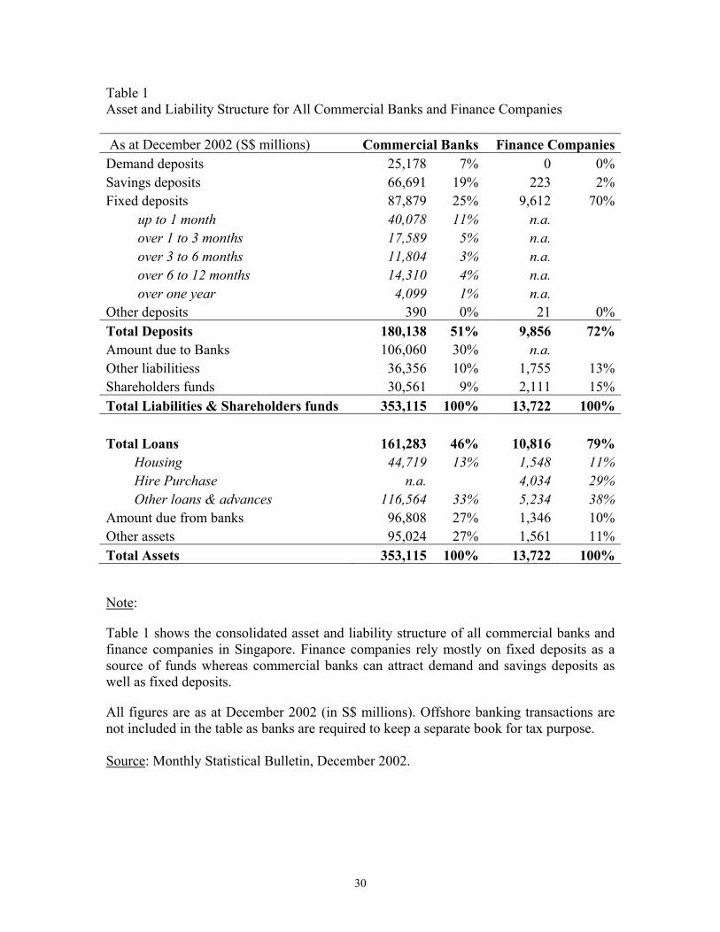
Table 1 Asset and Liability Structure for All Commercial Banks and Finance Companies As at December 2002 (S$ millions) Commercial Banks Finance CompaniesDemand deposits 25,178 7% 0 0%Savings deposits 66,691 19% 223 2%Fixed deposits 87,879 25% 9,612 70% up to 1 month 40,078 11% n.a. over 1 to 3 months 17,589 5% n.a. over 3 to 6 months 11,804 3% n.a. over 6 to 12 months 14,310 4% n.a. over one year 4,099 1% n.a. Other deposits 390 0% 21 0%Total Deposits 180,138 51% 9,856 72%Amount due to Banks 106,060 30% n.a. Other liabilitiess 36,356 10% 1,755 13%Shareholders funds 30,561 9% 2,111 15%Total Liabilities & Shareholders funds 353,115 100% 13,722 100% Total Loans 161,283 46% 10,816 79% Housing 44,719 13% 1,548 11% Hire Purchase n.a. 4,034 29% Other loans & advances 116,564 33% 5,234 38%Amount due from banks 96,808 27% 1,346 10%Other assets 95,024 27% 1,561 11%Total Assets 353,115 100% 13,722 100%
Note:
Table 1 shows the consolidated asset and liability structure of all commercial banks and finance companies in Singapore. Finance companies rely mostly on fixed deposits as a source of funds whereas commercial banks can attract demand and savings deposits as well as fixed deposits.
All figures are as at December 2002 (in S$ millions). Offshore banking transactions are not included in the table as banks are required to keep a separate book for tax purpose. Source: Monthly Statistical Bulletin, December 2002.
30
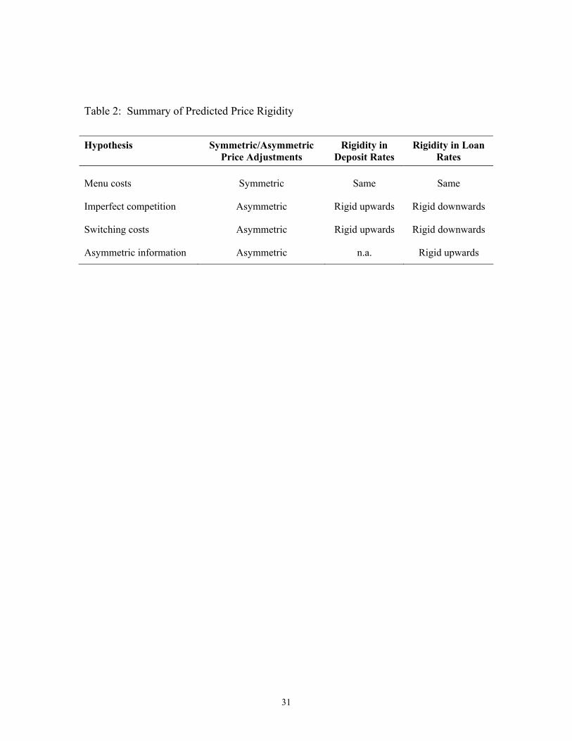
Table 2: Summary of Predicted Price Rigidity
Hypothesis Symmetric/Asymmetric
Price Adjustments Rigidity in
Deposit Rates Rigidity in Loan
Rates
Menu costs Symmetric Same Same
Imperfect competition Asymmetric Rigid upwards Rigid downwards
Switching costs Asymmetric Rigid upwards Rigid downwards
Asymmetric information Asymmetric n.a. Rigid upwards
31
Tabl
e 3
D
escr
iptiv
e St
atis
tics o
f the
Inte
rban
k R
ate
and
Adm
inis
tere
d In
tere
st R
ates
C
omm
erci
al B
anks
Fi
nanc
e C
ompa
nies
SIB
OR
Le
ndin
g R
ate
Dep
osit
Rat
es
Lend
ing
Rat
es
Dep
osit
Rat
es
3-m
onth
in
terb
ank
Prim
e ra
te
Savi
ngs
rate
3-
mon
th
Dep
osit
6-m
onth
D
epos
it 12
-mon
th
Dep
osit
Hire
Pu
rcha
se H
ousi
ng
Loan
Sa
ving
s ra
te
3-m
onth
D
epos
it 6-
mon
th
Dep
osit
12-m
onth
D
epos
it
Mea
n 0.
040
0.06
7 0.
03
0.03
5 0.
037
0.04
0.
078
0.07
5 0.
033
0.03
6 0.
039
0.04
3 M
edia
n
0.
036
0.06
30.
028
0.03
30.
037
0.04
0.07
40.
068
0.02
80.
032
0.03
60.
04 M
axim
um
0.08
40.
103
0.07
50.
076
0.07
60.
076
0.12
70.
124
0.07
90.
081
0.08
20.
082
Min
imum
0.
008
0.05
30.
004
0.00
80.
011
0.01
30.
051
0.06
10.
005
0.00
70.
010.
013
Std
. Dev
. 0.
019
0.01
2 0.
017
0.01
6 0.
015
0.01
5 0.
02
0.01
6 0.
018
0.01
7 0.
016
0.01
6
32

Tabl
e 4
C
orre
latio
n C
oeff
icie
nt a
mon
g th
e R
ates
PR
IME
BSA
VIN
G
BFD
3
BFD
6B
FD12
HP
HL
FSA
VIN
GFF
D3
FFD
6 FF
D12
SIB
OR
0.82
590.
8443
0.87
620.
8871
0.90
270.
7471
0.64
610.
8597
0.91
470.
9141
0.91
81PR
IME
0.
9370
0.95
310.
9516
0.93
910.
8592
0.88
060.
9185
0.94
740.
9487
0.93
32B
SAV
ING
0.
9502
0.94
700.
9451
0.90
590.
9036
0.98
830.
9577
0.95
590.
9528
BFD
30.
9976
0.98
820.
8716
0.82
230.
9301
0.98
880.
9884
0.97
84B
FD6
0.99
50 0.
8577
0.80
490.
9300
0.98
980.
9921
0.98
50B
FD12
0.84
000.
7845
0.93
210.
9873
0.99
220.
9927
HP
0.91
23
0.91
73
0.88
85
0.87
40
0.85
80H
L0.
8883
0.
8189
0.
8116
0.
7941
FSA
VIN
G
0.95
46
0.95
12
0.94
94FF
D3
0.99
80
0.99
12FF
D6
0.99
59N
otes
: PR
IME
= Pr
ime
rate
for c
omm
erci
al b
anks
. B
SAV
ING
= S
avin
gs ra
te fo
r ban
ks
BFD
3 =
3-m
onth
fixe
d (ti
me)
dep
osit
rate
for b
anks
B
FD6
= 6-
mon
th fi
xed
(tim
e) d
epos
it ra
te fo
r ban
ks
BFD
12 =
12-
mon
th fi
xed
(tim
e) d
epos
it ra
te fo
r ban
ks
HP
= H
ire-p
urch
ase
loan
rate
for f
inan
ce c
ompa
nies
H
L =
Hou
sing
loan
rate
for f
inan
ce c
ompa
nies
FS
AV
ING
= S
avin
gs ra
te fo
r fin
ance
com
pani
es
FFD
3 =
3-m
onth
fixe
d de
posi
t rat
e fo
r fin
ance
com
pani
es
FFD
6 =
6-m
onth
fixe
d de
posi
t rat
e fo
r fin
ance
com
pani
es
FFD
12 =
12-
mon
th fi
xed
depo
sit r
ate
for f
inan
ce c
ompa
nies
33
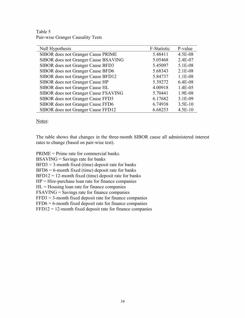
Table 5 Pair-wise Granger Causality Tests Null Hypothesis F-Statistic P-value SIBOR does not Granger Cause PRIME 5.48411 4.5E-08 SIBOR does not Granger Cause BSAVING 5.05468 2.4E-07 SIBOR does not Granger Cause BFD3 5.45097 5.1E-08 SIBOR does not Granger Cause BFD6 5.68343 2.1E-08 SIBOR does not Granger Cause BFD12 5.84737 1.1E-08 SIBOR does not Granger Cause HP 5.39272 6.4E-08 SIBOR does not Granger Cause HL 4.00918 1.4E-05 SIBOR does not Granger Cause FSAVING 5.70441 1.9E-08 SIBOR does not Granger Cause FFD3 6.17682 3.1E-09 SIBOR does not Granger Cause FFD6 6.74938 3.5E-10 SIBOR does not Granger Cause FFD12 6.68253 4.5E-10 Notes:
The table shows that changes in the three-month SIBOR cause all administered interest rates to change (based on pair-wise test). PRIME = Prime rate for commercial banks. BSAVING = Savings rate for banks BFD3 = 3-month fixed (time) deposit rate for banks BFD6 = 6-month fixed (time) deposit rate for banks BFD12 = 12-month fixed (time) deposit rate for banks HP = Hire-purchase loan rate for finance companies HL = Housing loan rate for finance companies FSAVING = Savings rate for finance companies FFD3 = 3-month fixed deposit rate for finance companies FFD6 = 6-month fixed deposit rate for finance companies FFD12 = 12-month fixed deposit rate for finance companies
34
Tabl
e 6
U
nit R
oot T
ests
on
leve
l and
firs
t diff
eren
ced
Serie
s
Le
vel
Crit
ical
Val
ues
1%
5%10
%SI
BO
RPr
ime
BFD
3B
FD6
BFD
12B
Savi
ngH
PH
LFF
D3
FFD
6FF
D12
FSav
ing
AD
F
-3
.458
-2.8
73-2
.573
-2.1
34-2
.253
-1.8
93-1
.954
-1.7
73-1
.542
-2.1
97-2
.607
-1.8
38-1
.908
-1.7
44-1
.542
PP
-3
.458
-2.8
73-2
.573
-2.2
02-2
.385
-1.9
00-1
.802
-1.7
14-1
.551
-2.2
03-3
.337
-1.8
54-1
.793
-1.7
31-1
.594
KPS
S0.
739
0.46
30.
347
1.23
80.
931
1.08
91.
101
1.15
81.
446
1.43
41.
104
1.27
41.
247
1.28
91.
632
Fi
rst-D
iffer
ence
d C
ritic
al V
alue
s
1%
5%
10%
SIB
OR
Prim
eB
FD3
BFD
6B
FD12
BSa
ving
HP
HL
FFD
3FF
D6
FFD
12FS
avin
g
AD
F
-3.4
58-2
.873
-2.5
73 -
14.6
17-8
.672
-8.3
60-8
.326
-8.5
00-8
.563
-9.5
64-6
.157
-8.3
37-8
.329
-8.4
70-8
.348
PP
-3.4
58-2
.873
-2.5
73 -
14.6
02
-8.7
16-8
.381
-8.3
26-8
.500
-8.5
25
-9.8
33-8
.744
-8.3
92-8
.329
-8.5
37-8
.342
KPS
S0.
739
0.46
30.
347
0.03
30.
094
0.06
10.
060
0.06
50.
085
0.07
80.
415
0.05
40.
059
0.06
40.
098
Not
es:
Bot
h A
DF
and
PP c
onsi
der u
nit-r
oot a
s the
nul
l hyp
othe
sis w
here
as K
PSS
uses
stat
iona
ry a
s the
nul
l hyp
othe
sis.
At 5
% le
vel o
f si
gnifi
canc
e, a
ll te
sts
indi
cate
that
all
the
serie
s ar
e un
it-ro
ot e
xcep
t for
the
PP te
st f
or H
L (i.
e., w
e ac
cept
the
null
hypo
thes
is f
or A
DF
and
PP te
sts
and
reje
ct th
e nu
ll hy
poth
esis
for
KPS
S). T
here
fore
, all
the
serie
s ca
n be
con
side
red
as u
nit r
oot
serie
s.
The
sam
e te
sts o
n fir
st-d
iffer
ence
d se
ries i
ndic
ate
that
all
the
serie
s are
stat
iona
ry (i
.e.,
we
reje
ct th
e nu
ll hy
poth
esis
for A
DF
and
PP
test
s and
acc
ept t
he n
ull h
ypot
hesi
s for
KPS
S).
35

Table 7
Cointegration Test
ADF Trace h=0
Trace h=1
Lambda Max h=0
Lambda Max h=1
Prime -3.169 29.593 5.211 24.382 5.211 BSaving -3.197 28.178 3.799 24.380 3.799 BFD3 -3.729 29.257 4.615 24.643 4.615 BFD6 -3.877 31.674 4.537 27.137 4.537 BFD12 -4.197 33.303 4.007 29.296 4.007
HP -2.814 26.795 4.801 21.994 4.801 HL -2.781 38.484 4.932 33.553 4.932
FSaving -3.466 33.648 3.897 29.751 3.897 FFD3 -4.583 36.146 4.311 31.835 4.311 FFD6 -4.569 36.115 4.249 31.866 4.249 FFD12 -4.714 34.430 3.799 30.632 3.799
Critical Values 1% -3.9618 24.6 24.6 20.2 20.2 5% -3.3654 19.96 19.96 15.67 15.67 10% -3.0657 17.58 17.58 13.75 13.75
Notes:
The ADF test is based on the residual from the simple regressions of administered rate variables on SIBOR (with constant). According to the ADF tests, HP and HL rates are not cointegrated with the SIBOR at 10% and Prime rate is not cointegrated with SIBOR at 5% (but cointegrated at 10%). However, Johansen’s Trace and Lambda-Max tests suggest that they are all cointegrated with the SIBOR. The Johansen’s test is considered more powerful than the Engle-Granger’s ADF test because the Johansen’s test does not require an arbitrary assignment of one of the series to be the left-hand side series.
36
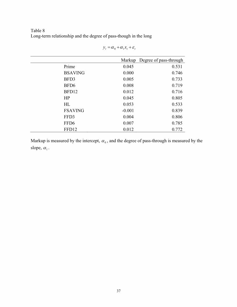
Table 8 Long-term relationship and the degree of pass-though in the long
ttt xy εαα ++= 10
Markup Degree of pass-through Prime 0.045 0.531 BSAVING 0.000 0.746 BFD3 0.005 0.733 BFD6 0.008 0.719 BFD12 0.012 0.716 HP 0.045 0.805 HL 0.053 0.533 FSAVING -0.001 0.839 FFD3 0.004 0.806 FFD6 0.007 0.785 FFD12 0.012 0.772
Markup is measured by the intercept, 0α , and the degree of pass-through is measured by the slope, 1α .
37
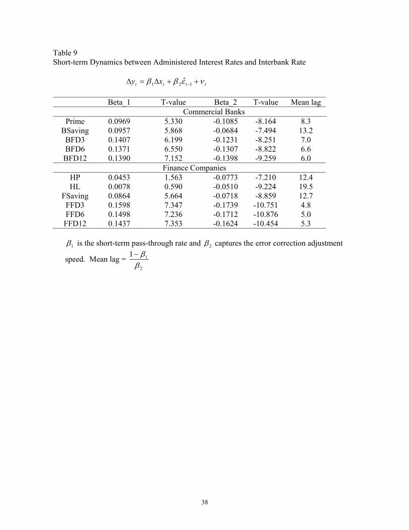
Table 9 Short-term Dynamics between Administered Interest Rates and Interbank Rate
tttt xy νεββ ++∆=∆ −121 ˆ
Beta_1 T-value Beta_2 T-value Mean lag
Commercial Banks Prime 0.0969 5.330 -0.1085 -8.164 8.3
BSaving 0.0957 5.868 -0.0684 -7.494 13.2 BFD3 0.1407 6.199 -0.1231 -8.251 7.0 BFD6 0.1371 6.550 -0.1307 -8.822 6.6 BFD12 0.1390 7.152 -0.1398 -9.259 6.0
Finance Companies HP 0.0453 1.563 -0.0773 -7.210 12.4 HL 0.0078 0.590 -0.0510 -9.224 19.5
FSaving 0.0864 5.664 -0.0718 -8.859 12.7 FFD3 0.1598 7.347 -0.1739 -10.751 4.8 FFD6 0.1498 7.236 -0.1712 -10.876 5.0 FFD12 0.1437 7.353 -0.1624 -10.454 5.3
1β is the short-term pass-through rate and 2β captures the error correction adjustment
speed. Mean lag = 2
1
β1 β−
38
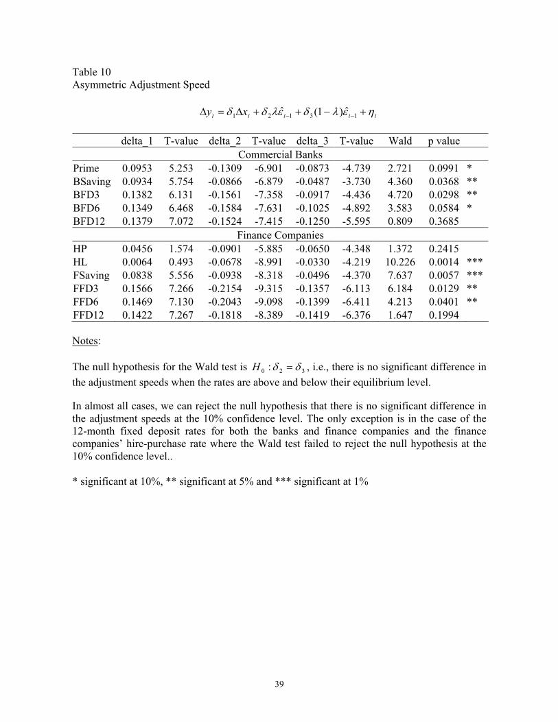
Table 10 Asymmetric Adjustment Speed ttttt xy ηελδελδδ +−++∆=∆ −− 13121 ˆ)1(ˆ delta_1 T-value delta_2 T-value delta_3 T-value Wald p value
Commercial Banks Prime 0.0953 5.253 -0.1309 -6.901 -0.0873 -4.739 2.721 0.0991 * BSaving 0.0934 5.754 -0.0866 -6.879 -0.0487 -3.730 4.360 0.0368 ** BFD3 0.1382 6.131 -0.1561 -7.358 -0.0917 -4.436 4.720 0.0298 ** BFD6 0.1349 6.468 -0.1584 -7.631 -0.1025 -4.892 3.583 0.0584 * BFD12 0.1379 7.072 -0.1524 -7.415 -0.1250 -5.595 0.809 0.3685
Finance Companies HP 0.0456 1.574 -0.0901 -5.885 -0.0650 -4.348 1.372 0.2415 HL 0.0064 0.493 -0.0678 -8.991 -0.0330 -4.219 10.226 0.0014 *** FSaving 0.0838 5.556 -0.0938 -8.318 -0.0496 -4.370 7.637 0.0057 *** FFD3 0.1566 7.266 -0.2154 -9.315 -0.1357 -6.113 6.184 0.0129 ** FFD6 0.1469 7.130 -0.2043 -9.098 -0.1399 -6.411 4.213 0.0401 ** FFD12 0.1422 7.267 -0.1818 -8.389 -0.1419 -6.376 1.647 0.1994 Notes: The null hypothesis for the Wald test is 320 : δδ =H , i.e., there is no significant difference in the adjustment speeds when the rates are above and below their equilibrium level.
In almost all cases, we can reject the null hypothesis that there is no significant difference in the adjustment speeds at the 10% confidence level. The only exception is in the case of the 12-month fixed deposit rates for both the banks and finance companies and the finance companies’ hire-purchase rate where the Wald test failed to reject the null hypothesis at the 10% confidence level.. * significant at 10%, ** significant at 5% and *** significant at 1%
39

40
Table 11 Mean adjustment lags (MAL) in months
Symmetric Model Asymmetric Model Above the mean Below the Mean
Commercial Banks Prime 8.3 6.9 10.4
BSaving 13.2 10.5 18.6 BFD3 7.0 5.5 9.4 BFD6 6.6 5.5 8.4 BFD12 6.2 5.7 6.9
Finance Companies HP 12.4 10.6 14.7 HL 19.5 14.7 30.1
FSaving 12.7 9.8 18.5 FFD3 4.8 3.9 6.2 FFD6 5.0 4.2 6.1 FFD12 5.3 4.7 6.0
Top Related