


Languages
Pages
Legal

A A2182NTATION PAGE FO"A0rvo
OD,2 8TE 1.. REPO - 0"1. W____ _me. 070d-01Noll~v to6,4, 0rW 19 ~W I CulW6." 199nto-JCme 9V 0. 1992ft
4. TITLE AND SUJU1IUl S. FUNDING NUMIIERSBayesian Cross-Entropy Reconstruction of N00014-91-J-4056
Complex Images
I. AUThOR(S)B. Roy Frieden PROM~OGNZTO
The University of Arizona*- nvlOft a t*O
Optical Sciences Center MARO 9199"Tucson, Arizona 85721 C
4. SPOTSOIANG / MONITORING AGENCY NAMS(S) AND ADOhESS(ES) 10. SPONSORING / MONTORBING• ~AGENCY REPORT NUMEERIDepartment of the NavyC
Office of Naval ResearchResident Representative
~~I I U
127. OIGSTRIUTION / AVAI MEILI $ STATEMENTr 12.k DITFOM-TON CODE
approved for public release; distribution unlimited
". AOSTaCT (Mazcimum 200 wOMAl
u98 3 8 157SBajkova's generalized maximum entropy method (GMEM) for reconstruction of complex
psignals has been further generalized through the use of KuNlback-Leibler cross entropy.This permits a priori information in the form of bias functions to be inserted into the
e algorithm, with resulting benefits to reconstruction quality. Also, the cross-entropy term
O • is imbedded within an overall m.a.p. (maximum a posteriori probability) approach thatI mR includes a noise-rejection term. A further modification is transformation of the large,)U e two-dimensional problem due to modest-sized 2-D images into a sequence of one-0'C dimensional problems. Finally, the added operation of three-point median window
__ w filtration of each intermediary, one-dimensional output is shown to suppress edge-topovershoots while augmenting edge gradients. Applications to simulated complex images
are shown.
14. SUgIECT TEIRMs ¶S. NM;ERl oP PAGES32
ilII PCI CODEI
17. SECURIrY CLASSiFICATION 13. SECUtUITY CLASSIFICAT1ON II. SECURITY a]ASSWICAIONm N. LIIATION OP ASSTRACTiOf RAPOT OF A2STlRACTunclassified f unclassified t unclassified n/a
NSAI 754041.2510-S500 Stt4r Poe 293 (N, w 29-,
Q M ~ ~ ~ ~ ~ ~ ~ ~ ~ ~ ~ ~ ~ ~ ~~~~~~•I I~sprisapir nomto ntefr fba ucin ob neteino th

Bayesian Cross-Entropy Reconstruction of Complex Images
B. Roy Frieden
Optical Sciences Center, The University of Arizona
Tucson, Arizona 85721
Anisa T. Bajkova
Institute of Applied Astronomy of the USSR Academy of Sciences
St. Petersburg 197042, Russia
Abstract
Balkova's generalized maximum entropy method (GMEM) for reconstruction of complex
signals has been further generalized through the use of Kullback-Leibler cross entropy. This
permits a priori information in the form of bias functions to be inserted into the algorithm, with
resulting benefits to reconstruction quality. Also, the cross-entropy term is imbedded within
an overall m.a.p. (maximum a posteriori probability) approach that includes a noise-rejection
term. A further modification is transformation of the large, two-dimensional problem due to
modest-sized 2-D images into a sequence of one-dimensional problems. Finally, the added
operation of three-point median window filtration of each intermediary, one-dimensional
output is shown to suppress edge-top overshoots while augmenting edge gradients.
Applications to simulated complex images are shown.
ByD Di.tributicn/Avail abillty Codes
Avail anid/or
at SpeciL&
m. L
Introduction
Complex signals occur widely in electromagnetic phenomena. It is often required to
estimate such signals from incomplete data in a conjugate space. As examples: In interactive
synthetic aperture radar (ISAR)' the complex Fourier transform of a spatial amplitude image
is known within a band of frequencies, and from this data the complex image is to be
estimated. In radio astronomy, the data are complex amplitudes in an unfilled Fourier space
as dictated by the earth's motion2 . In Fourier transform holography, the hologram might
have missing or damaged regions. In quantum mechanics, the spatial wave function of a
particle is to be estimated from incomplete knowledge of momentum (Fourier) space for the
particle. In these examples, the conjugate space to the required signal is Fourier space.
Although the processing approach described below applies to any linear conjugate space,
because of its central importance we will continue the development specifically for the
Fourier-space problem. Because of the incomplete knowledge of Fourier space we seek a
processing approach that allows for bandwidth interpolation and extrapolation.
Entropic Processing
Since its first use in image restoration 3 , maximum entropy has been known to be
capable of extrapolation in Fourier space. It also produces maximally smooth, or unbiased,
estimates 3 '4 . If f(t) is a real signal to be estimated, then the maximum entropy solution f(t)
is to satisfy
- f dt f(t) In f(t) a H - Max., f(t) -t, (1)
subject to constraints on f(t) provided by the Fourier data. (All integrals have infinite limits
2

unless otherwise specified.) Quantity H is the (real) Shannon entropy of the signal. As noted,
the signal must be real and positive-definite for a real H to exist. Methods of achieving
maximum entropy estimation in different senses than (1) also exist. Among these are
Burg'ss In x(t)-form of entropy and Borden's 6 probabilistic model approach. In this paper, we
stick with form (1) of entropy because of its widespread use in signal estimation problems 7.
The formulation (1) of maximum entropy has, in the past, been exclusively applied to
positive-definite, real signals such as probability densities 8 , power spectra5 , and intensity
images 3'9 . However, here we want to work with the Shannon entropy of a complex signal.
How can this be done?
Recently, Bajkova10 showed how to accomplish this objective. We describe her
approach first, and then formulate an improved version for application to noisy, two-
dimensional complex images.
GMEM Processing
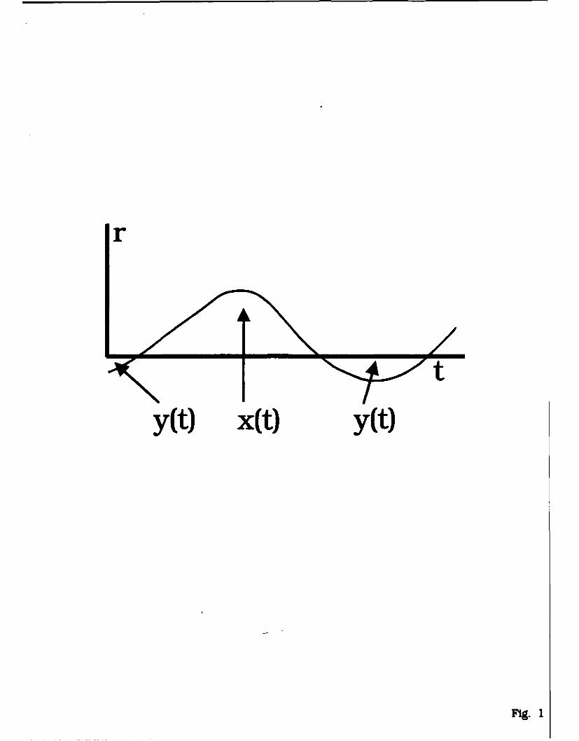
First, consider a real signal r(t), as in Fig. 1, that is to be estimated. It is generally
bipolar, with positive and negative values as indicated. Such a signal can be represented as
the difference between two positive-definite functions
r(t) = x(t) - y(t), x(t) > O, y(t) a O. (2)
Thus, the positive regions in Fig. 1 are represented by r(t), the negative by y(t). Curves x(t)
and y(t) do not, of course, have overlapping support regions. Let us replace the problem of
estimating r(t) by one of estimating x(t) and y(t). Then for any estimates of x(t), y(t) to be
valid, they must have non-overlapping support regions and must be positive-definite.
3
The latter constraint allows the entropy
-f dt x(t) In x(t) - dt y(t) In y(t) (3a)
to exist. Hence, maximum entropy processing can be applied to these signals, aiding our
overall objective. Furthermore, since x(t) and y(t) do not overlap, the entropy integral (3a) is
the entropy of the absolute value of r(t) as well,
-Jdtlr(t) I/n Ir(t)I "H(r). (3b)
Thus, maximizing the entropy H(r) is equivalent to maximizing the sum of the entropies of x(t)
and y(t). This would allow each constituent x(t), y(t) of the required signal r(t) to be
separately estimated by maximum entropy. Again, this is despite the fact that r(t) may have
negative regions. Hence, we adapt the maximization of (3b) as our criterion.
The extension to the full-blown complex problem is straightforward. Consider a
complex signal
u(t) = r(t) +jq(t), j = ,(4)
r(t), q(t) real and generally bipolar. We wish to estimate u(t). Equivalently, we may choose
to estimate r(t) and q(t). Represent r(t) as in Eq. (2), and similarly represent
q(t) = z(t) - v(t), z(t) O, v(t) O. (5)
The entropy of the absolute value of r(t) still obeys both Eqs. (3a,b). Likewise the entrdpy of
the absolute value of q
4
H(q) -dt I q(t) I In I q(t)I (6)
also obeys
H(q) = -Jdt z(t) In z(t) - f dt v(t) In v(t), (7)
providing z(t), v(t) do not overlap. Hence, maximizing the entropy H(q) accomplishes an
entropic estimate of q(t).
Since our objective is to estimate the complex u(t), we have to estimate both real and
imaginary parts r(t) and q(t). This suggests that we adopt one grand principle of maximizing
the sumtotal entropy H(r) plus H(q), or
H(u) - H(r) + H(q)
= -f dtlx(t) In x(t) + y(t) In y(t) + z(t) Inz(t) vt) In v(t)
= Max. (8)
Next, recall the nonoverlapping support requirements for x(t), y(t) and for z(t), v(t).
This would not necessarily be met by simply maximizing the form (8). It was empirically
found7 that a 'tuning parameter' a must be inserted, to form an associated entropy
H(u;a) - -J dt {x(t) In [ax(t)] + y(t) In(ay(t)] + z(t) In [oz(t)] + v(t) In [av(t)] }.J (9)
= Max.
The value of a is at the discretion of the user. Empirically, the action of a is to force
nonoverlap as a is made larger. Also, a large a causes better data agreement and, hence,
higher resolution in the output u(t). This is because the principle (9) will be constrained by
5
higher resolution in the output u(t). This is because the principle (9) will be constrained by
input data as well, and the data are more closely obeyed when mathematical constructions
(2) and (5) for r(t) and q(t) are valid (i.e., when the functions do not overlap). This was
empirically borne out by computer simulations described below.
GMEMK Processing
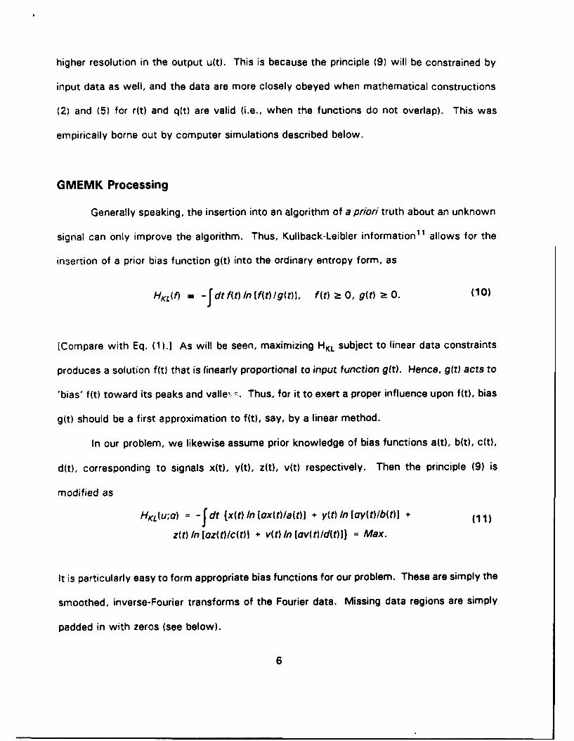
Generally speaking, the insertion into an algorithm of a priori truth about an unknown
signal can only improve the algorithm. Thus, Kullback-Leibler information1 1 allows for the
insertion of a prior bias function g(t) into the ordinary entropy form, as
HKL(f) m - dtf(t)In[f(t)lg(t)], ftW 2t 0, g(t) - 0. (10)
[Compare with Eq. (1).] As will be seen, maximizing HKL subject to linear data constraints
produces a solution f(tj that is linearly proportional to input function g(t). Hence, g(t) acts to
'bias' f(t) toward its peaks and vallei-.. Thus, for it to exert a proper influence upon f(t), bias
g(t) should be a first approximation to f(t), say, by a linear method.
In our problem, we likewise assume prior knowledge of bias functions a(t), b(t), c(t),
d(t), corresponding to signals x(t), y(t), z(t), v(t) respectively. Then the principle (9) is
modified as
HKL(u;a) = -Jdt {x(t) In [ax(t)la(t)] + y(t) In [ay(t)lb(t)] + 011)
z(t) In [az(tct)] + v(t) In [ov(t)/d(t)]} = Max.
It is particularly easy to form appropriate bias functions for our problem. These are simply the
smoothed, inverse-Fourier transforms of the Fourier data. Missing data regions are simply
padded in with zeros (see below).
6
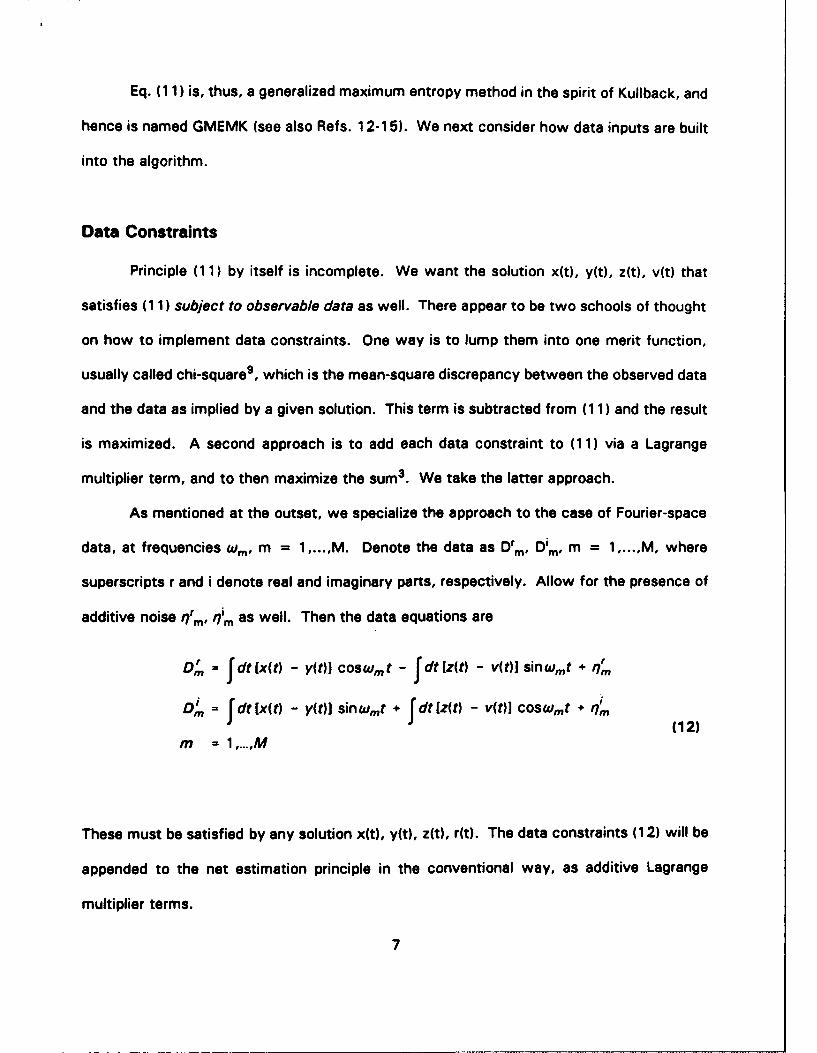
Eq. (11) is, thus, a generalized maximum entropy method in the spirit of Kullback, and
hence is named GMEMK (see also Refs. 1 2-1 5). We next consider how data inputs are built
into the algorithm.
Data Constraints
Principle (11) by itself is incomplete. We want the solution x(t), y(t), z(t), v(t) that
satisfies (1 1) subject to observable data as well. There appear to be two schools of thought
on how to implement data constraints. One way is to lump them into one merit function,
usually called chi-square9, which is the mean-square discrepancy between the observed data
and the data as implied by a given solution. This term is subtracted from (11) and the result
is maximized. A second approach is to add each data constraint to (1 1) via a Lagrange
multiplier term, and to then maximize the sum 3 . We take the latter approach.
As mentioned at the outset, we specialize the approach to the case of Fourier-space
data, at frequencies Win, m = 1,..., M. Denote the data as Drm, D im, m = 1,...,M, where
superscripts r and i denote real and imaginary parts, respectively. Allow for the presence of
additive noise qrm, i7'rn as well. Then the data equations are
D = f dt [x(t) - y(t)] coswmt - Jfdt [z(t) - v(t)] sinwmt + i74
D= J fdt [x(t) - y(t)J sinwm..t + J dt fz(t) -v(t)J coswmt + (12)
m =1...M
These must be satisfied by any solution x(t), y(t), z(t), r(t). The data constraints (1 2) will be
appended to the net estimation principle in the conventional way, as additive Lagrange
multiplier terms.
7
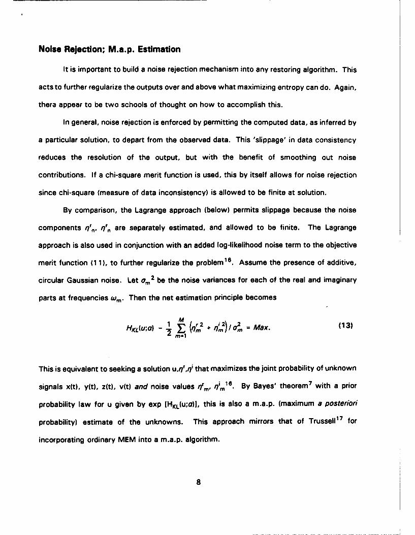
Noise Rejection; M.a.p. Estimation
It is important to build a noise rejection mechanism into any restoring algorithm. This
acts to further regularize the outputs over and above what maximizing entropy can do. Again,
thera appear to be two schools of thought on how to accomplish this.
In general, noise rejection is enforced by permitting the computed data, as inferred by
a particular solution, to depart from the observed data. This 'slippage' in data consistency
reduces the resolution of the output, but with the benefit of smoothing out noise
contributions. If a chi-square merit function is used, this by itself allows for noise rejection
since chi-square (measure of data inconsistency) is allowed to be finite at solution.
By comparison, the Lagrange approach (below) permits slippage because the noise
components qrt , r/rn are separately estimated, and allowed to be finite. The Lagrange
approach is also used in conjunction with an added log-likelihood noise term to the objective
merit function (1 1), to further regularize the problem 16 . Assume the presence of additive,
circular Gaussian noise. Let am 2 be the noise variances for each of the real and imaginary
parts at frequencies Wim. Then the net estimation principle becomes
Ma
This is equivalent to seeking a solution u,q",q' that maximizes the joint probability of unknown
signals x(t), y(t), z(t), v(t) and noise values frm, rira' 6*. By Bayes' theorem 7 with a prior
probability law for u given by exp [HKL(U;0)], this is also a m.a.p. (maximum a posteriori
probability) estimate of the unknowns. This approach mirrors that of Trussell1 7 for
incorporating ordinary MEM into a m.a.p. algorithm.
8
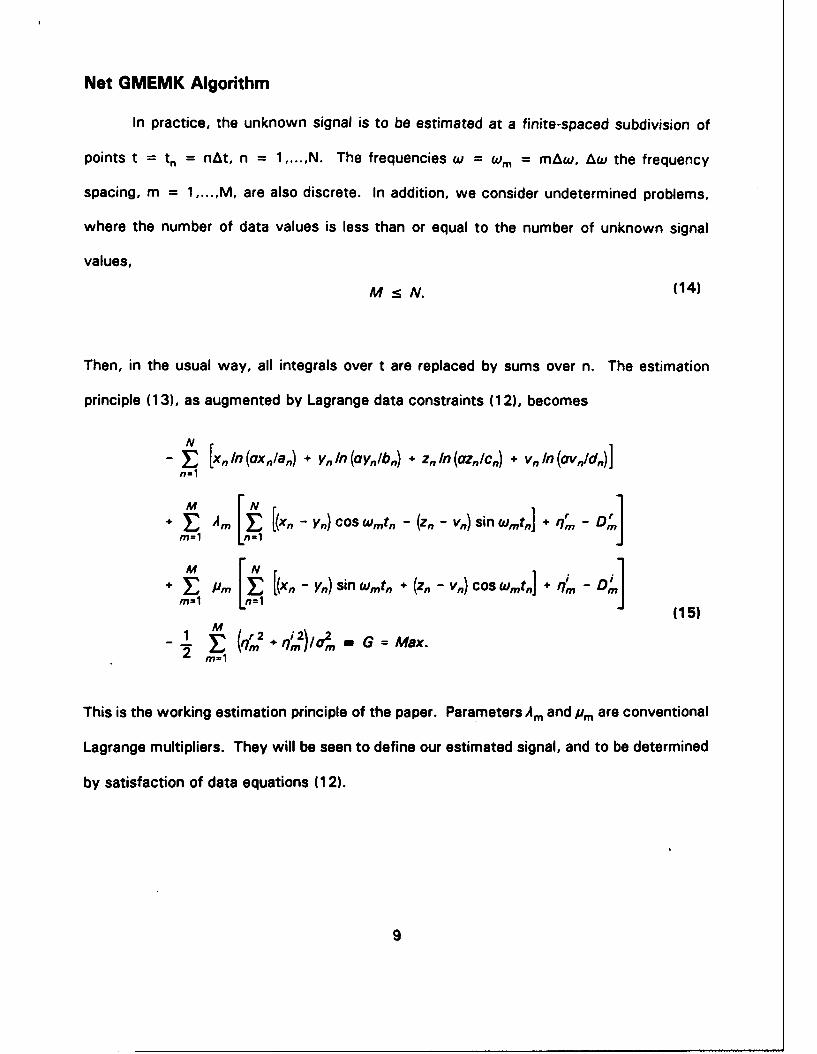
Net GMEMK Algorithm
In practice, the unknown signal is to be estimated at a finite-spaced subdivision of
points t = tn = nAt, n = 1,...,N. The frequencies w = wm = mAw, Aw the frequency
spacing, m = 1 ,.... ,M, are also discrete. In addition, we consider undetermined problems,
where the number of data values is less than or equal to the number of unknown signal
values,
M s N. (14)
Then, in the usual way, all integrals over t are replaced by sums over n. The estimation
principle (13), as augmented by Lagrange data constraints (1 2), becomes
- N [x,1n(axia,) + yIn ayib,,) + zIn(azic÷) + vIn av~Id,)]
n-1
M- It~ [(xn - cos COW&mtn - (zn -V.) sinl &mtn + a" Am ]
Pm= It[n - Y.7) sin wmt,, + -z v17) cos Wmtn,] + i& - Dm'j 15
E (7r2 12)/a = G = Max.2rn-i
This is the working estimation principle of the paper. Parameters Am and Pm are conventional
Lagrange multipliers. They will be seen to define our estimated signal, and to be determined
by satisfaction of data equations (12).
9
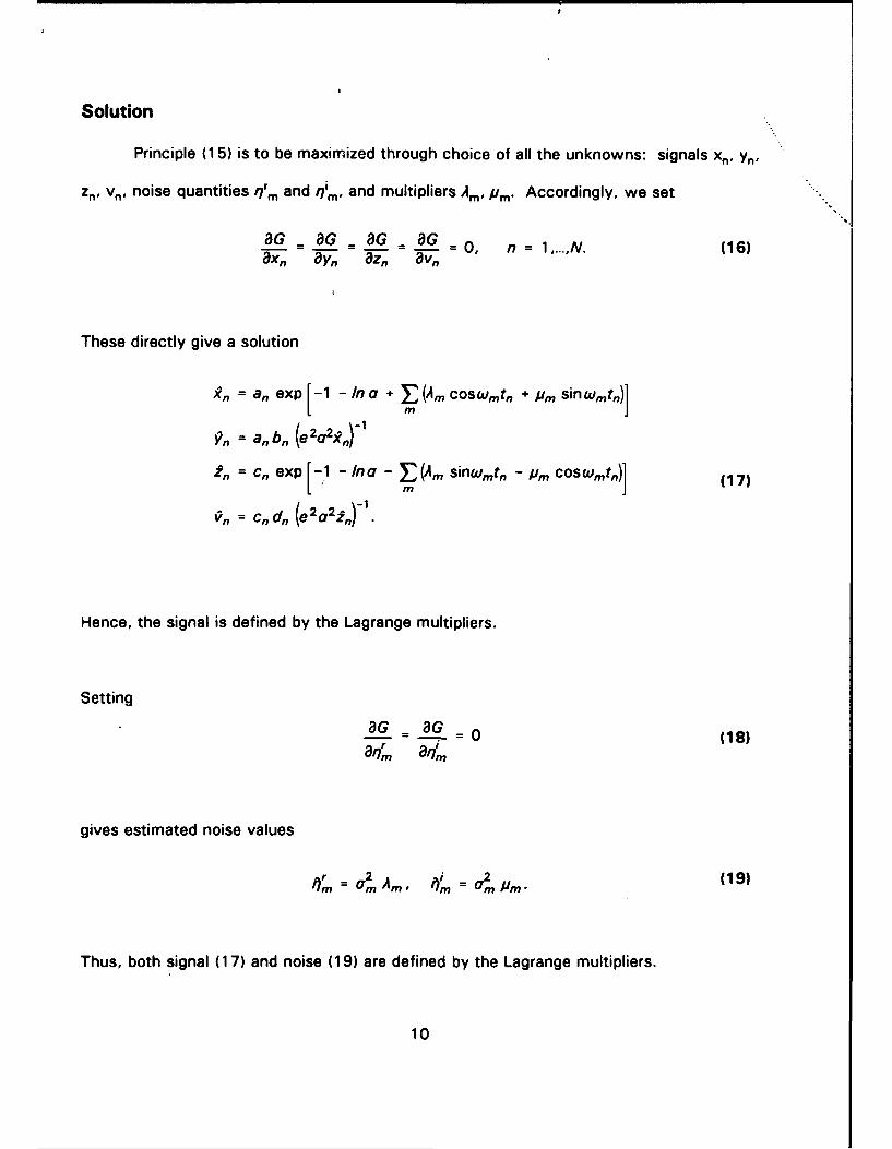
Solution
Principle (1 5) is to be maximized through choice of all the unknowns: signals xn, Yn,
zn, vn, noise quantities rirm and q'm, and multipliers Am, /rM " Accordingly, we set
aG - 8G - aG - aG - 0, n = 1 ....N. (16)axn ay, az, avn
These directly give a solution
,n= an exp [-1 In a + E (Am coswmtn + jim sinwmtn)]I- mJ
9,, = an,,b, (e2a2g,,r1
2, = cn exp [-1 -Ina - (Am sinwmt,- Pm COSwmtn)] (17)
Cn = Cndn (e2a24n)Y1 .
Hence, the signal is defined by the Lagrange multipliers.
Setting
G- G 0 (18)
aq,7 a, ,,
gives estimated noise values
•r = 0,2 A'/i= 0,2 P" (19)
Thus, both signal (1 7) and noise (19) are defined by the Lagrange multipliers.
10
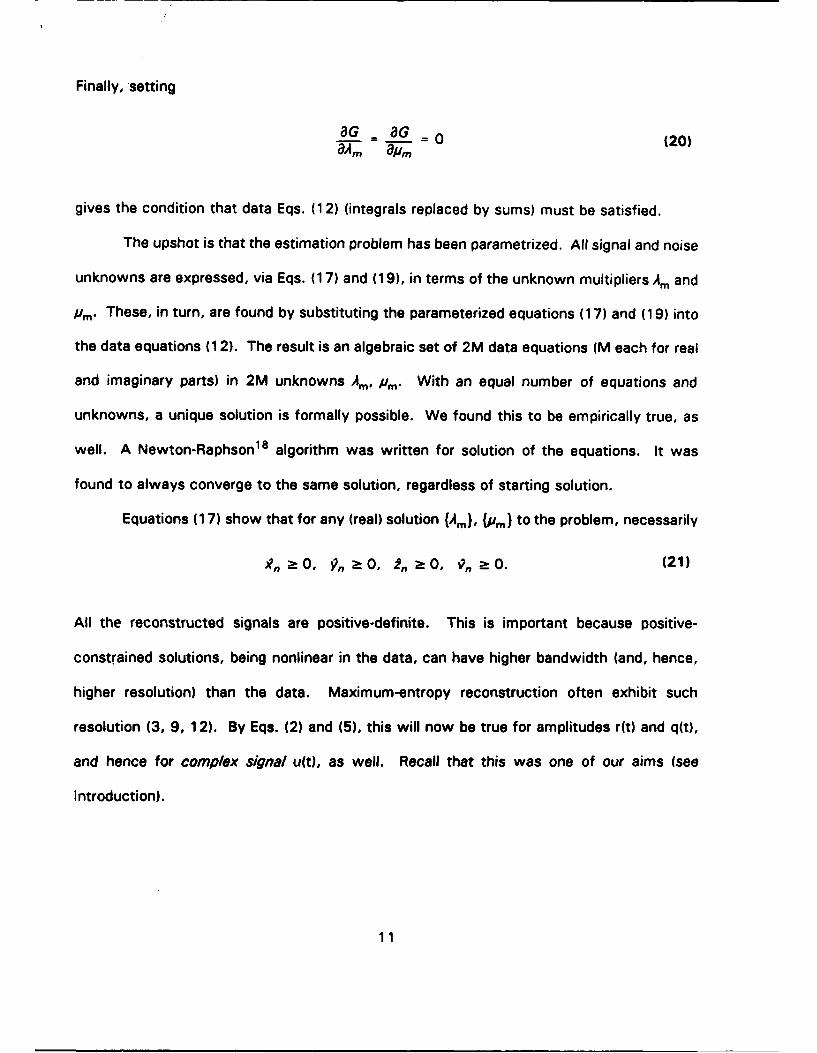
Finally, 'setting
aG aG = 0 (20)
gives the condition that data Eqs. (1 2) (integrals replaced by sums) must be satisfied.
The upshot is that the estimation problem has been parametrized. All signal and noise
unknowns are expressed, via Eqs. (1 7) and (19), in terms of the unknown multipliers Am and
/Pm" These, in turn, are found by substituting the parameterized equations (17) and (19) into
the data equations (1 2). The result is an algebraic set of 2M data equations (M each for real
and imaginary parts) in 2M unknowns Am, Pro" With an equal number of equations and
unknowns, a unique solution is formally possible. We found this to be empirically true, as
well. A Newton-Raphsonia algorithm was written for solution of the equations. It was
found to always converge to the same solution, regardless of starting solution.
Equations (1 7) show that for any (real) solution (Am), (Pm) to the problem, necessarily
,?n a>0, 9n 20, 2n 20, On :t0. (21)
All the reconstructed signals are positive-definite. This is important because positive-
constrained solutions, being nonlinear in the data, can have higher bandwidth (and, hence,
higher resolution) than the data. Maximum-entropy reconstruction often exhibit such
resolution (3, 9, 12). By Eqs. (2) and (5), this will now be true for amplitudes r(t) and q(t),
and hence for complex signal u(t), as well. Recall that this was one of our aims (see
Introduction).
11

Two-dimensional implementation as sequence of 1-D problems
The notation has, so far, been one-dimensional. In principle, two dimensional data
Drmn, Dmn, can be processed by the straightforward double-subscripting of all single-
subscripted quantities above. However, the result would be a requirement to solve (now) 2M 2
data equations in 2M 2 unknowns, a formidable problem for even modest-sized pictures of
M - 64 pixels on a side.
A way to surmount this problem of implementation is to break up the one, two-
dimensional problem into a sequence of one-dimensional problems. Note that the Fourier data
problem under consideration has a separable imaging kernel
exp [j(W1 tl + W2 t 2 )] = exp (jwl tl) • exp (jw 2 t 2 ), (22)
where t1 denotes (now) row coordinate and t2 denotes column coordinate. The 2-D problem
f f dtidt2 u(tl,t 2) eJ(WIt , + 1212t) = D(w1 ,W2 ) (23)
of estimating u(t 1 , t 2) may then be re-cast as
f dtleiw( t' E(tl;w2 ) = D(w,;W2)' (24a)
where
f dt2 eJ W2t2 U(t 1, t2 ) = E(tl ; W2 ). (24b)
This implies the following procedure for obtaining a solution u(t 1, t2).
12

First solve Eq. (24a) for the complex quantity E(tl; •2 ) at each (row) W2 = mAw, m
= 1 ,... ,M. This is a sequence of M 1--D problems of size 2M. The solutions E(tl; w2 ) are
stored in an intermediary matrix. These are then used to form the right-hand sides of Eq.
(24b), which is then solved for u(t 1, t2 ) at each (column) t2 = nAt, n = 1,...,N. This is a
sequence of N 1 -D problems of size 2M. The net effect is that the original 2-D problem of
2M2 unknowns in 2M2 equations is replaced by (M + N) one-dimensional problems of size 2M
each. This procedure was followed below.
Demonstrations
Fourier images were formed, and processed, on a Convex C240 mini-super computer.
The object was always the 64x64 pixel airplane silhouette shown in Fig. 2. This is a complex
signal of real-part + 1 and imaginary part -1 within the airplane outline, and 0 outside. All
images show the modulus signal. This is usually the output of interest, e.g., in ISAR (inverse
synthetic aperture radar) images. Note also the point source to the right of the airplane nose
in Fig. 2. Edges and point sources are strong carriers of pattern shape information, and hence
are crucial for purposes of pattern recognition. Overall, then, this image is contrived to test
the GMEMK algorithm on a combined edge-point source object input.
The general objective was to form Fourier data from the complex object in Fig. 2, both
without and with noise, and to observe the ability of the GMEMK algorithm to reconstruct the
object under these conditions. Also, to more critically test the algorithm, we blanked out half
the frequency-space of data values, and so attempted to reconstruct on a twice-as-fine basis
as the data would ordinarily permit. Hence, we attempted bandwidth extrapolation, by a
factor of two, in both resolution directions.
13

As will be discussed, the GMEMK algorithm can be augmented by a median window
filter step, after each row or column reconstruction, so as to suppress Gibbs artifact oscil-
lations that are induced by GMEMK (or any other reconstruction algorithm) at the edge tops.
Noise free data
The first demonstration is a noise-free one. The 64x64 pixel complex object of Fig.
2 is Fourier transformed, to give the spectrum shown in Fig. 3. The logarithm of the modulus
is displayed for better viewing.
The black picture frame indicates blanked out data. Only the central 32x32 spectral
values shown are used as data inputs to GMEMK. However, the reconstruction will still be
on the 64x64 pixel basis. The aim is to regain the resolution apparently lost by blanking out
the picture frame data values.
The conventional, linear output for the problem is first shown. This is the inverse,
discrete Fourier transform (DFT) of the data. For example, in ISAR imaging, after the data are
estimated in Fourier space, a DFT is ordinarily performed to produce the output image in direct
space1 . The picture frame region of unknown data was accommodated by simply assuming
that all values are zero there. This 'zero padding' method is the usual one for artificially in-
creasing output picture size using the DFT. The DFT of the data in Fig. 3 is shown in Fig. 4.
In this noise-free case, noise throughput in Fig. 4 is not a problem, but there is a
notable loss of resolution at the airplane edges, and of the isolated point source. Of course
this is due to loss of the outer frequencies (picture frame) in data space. Note also the artifact
oscillations immediately around the airplane. These are also caused by the missing
frequencies.
14
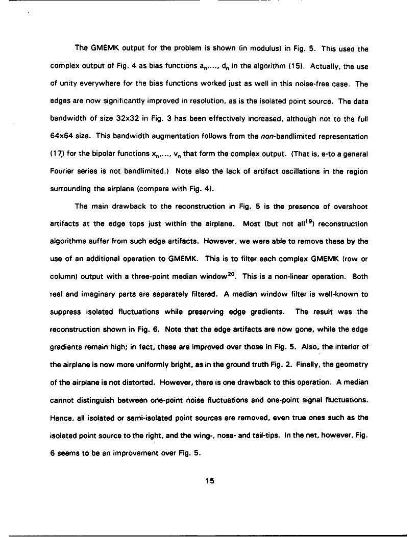
The GMEMK output for the problem is shown (in modulus) in Fig. 5. This used the
complex output of Fig. 4 as bias functions an ..... d, in the algorithm (15). Actually, the use
of unity everywhere for the bias functions worked just as well in this noise-free case. The
edges are now significantly improved in resolution, as is the isolated point source. The data
bandwidth of size 32x32 in Fig. 3 has been effectively increased, although not to the full
64x64 size. This bandwidth augmentation follows from the non-bandlimited representation
(17) for the bipolar functions xn,...., vn that form the complex output. (That is, e-to a general
Fourier series is not bandlimited.) Note also the lack of artifact oscillations in the region
surrounding the airplane (compare with Fig. 4).
The main drawback to the reconstruction in Fig. 5 is the presence of overshoot
artifacts at the edge tops just within the airplane. Most (but not all19 ) reconstruction
algorithms suffer from such edge artifacts. However, we were able to remove these by the
use of an additional operation to GMEMK. This is to filter each complex GMEMK (row or
column) output with a three-point median window 20 . This is a non-linear operation. Both
real and imaginary parts are separately filtered. A median window filter is well-known to
suppress isolated fluctuations while preserving edge gradients. The result was the
reconstruction shown in Fig. 6. Note that the edge artifacts are now gone, while the edge
gradients remain high; in fact, these are improved over those in Fig. 5. Also, the interior of
the airplane is now more uniformly bright, as in the ground truth Fig. 2. Finally, the geometry
of the airplane is not distorted. However, there is one drawback to this operation. A median
cannot distinguish between one-point noise fluctuations and one-point signal fluctuations.
Hence, all isolated or semi-isolated point sources are removed, even true ones such as the
isolated point source to the right, and the wing-, nose- and tail-tips. In the net, however, Fig.
6 seems to be an improvement over Fig. 5.
15
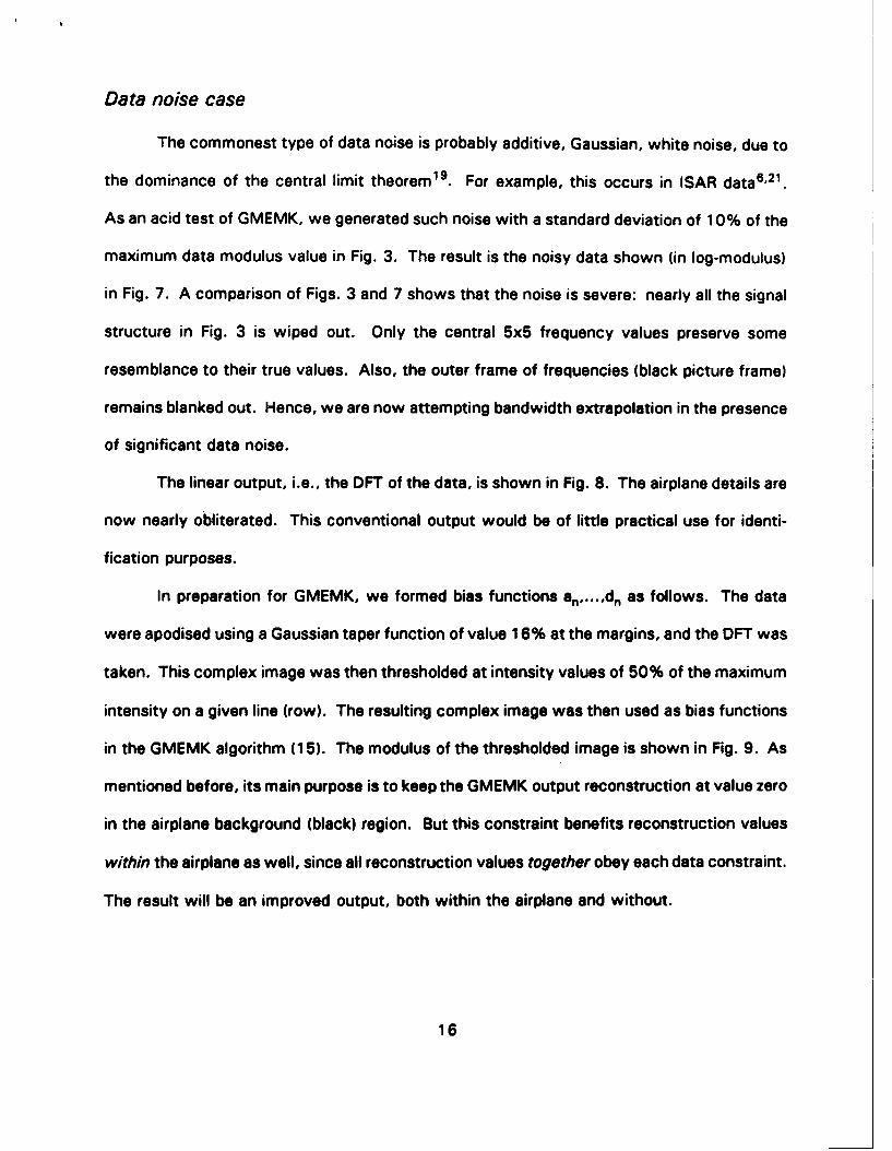
Data noise case
The commonest type of data noise is probably additive, Gaussian, white noise, due to
the dominance of the central limit theorem"9 . For example, this occurs in ISAR data6 ,2 1.
As an acid test of GMEMK, we generated such noise with a standard deviation of 10% of the
maximum data modulus value in Fig. 3. The result is the noisy data shown (in log-modulus)
in Fig. 7. A comparison of Figs. 3 and 7 shows that the noise is severe: nearly all the signal
structure in Fig. 3 is wiped out. Only the central 5x5 frequency values preserve some
resemblance to their true values. Also, the outer frame of frequencies (black picture frame)
remains blanked out. Hence, we are now attempting bandwidth extrapolation in the presence
of significant data noise.
The linear output, i.e., the DFT of the data, is shown in Fig. 8. The airplane details are
now nearly obliterated. This conventional output would be of little practical use for identi-
fication purposes.
In preparation for GMEMK, we formed bias functions an,.... dn as follows. The data
were apodised using a Gaussian taper function of value 16% at the margins, and the DFT was
taken. This complex image was then thresholded at intensity values of 50% of the maximum
intensity on a given line (row). The resulting complex image was then used as bias functions
in the GMEMK algorithm (15). The modulus of the thresholded image is shown in Fig. 9. As
mentioned before, its main purpose is to keep the GMEMK output reconstruction at value zero
in the airplane background (black) region. But this constraint benefits reconstruction values
within the airplane as well, since all reconstruction values together obey each data constraint.
The result will be an improved output, both within the airplane and without.
16
The GMEMK-median window output is shown in Fig. 10. Comparison with the linear
reconstruction of Fig. 8 shows a strong improvement in image fidelity. The background lacks
noise, the airplane outline is more faithfully reconstructed, and the structure within the
airplane is more uniform.
It is important, also, to compare entropy output Fig. 10 with the linear, bias image of
Fig. 9. If output Fig. 10 closely resembled Fig. 9, this would indicate that the entropy
algorithm did little over and above the linear, thresholding operation of Fig. 9 to improve the
image. For example, if both figures showed the same airplane boundaries this would mean
that the subjectively chosen thresholding level was crucial to the quality of the entropy
reconstruction. This would be an unsatisfactory result. However, a comparison of Figs. 9
and 10 shows, to the contrary, that the airplane boundaries in the entropy reconstruction are
significantly drawn inward from their bias image values, toward the true boundary values (of
Fig. 2). Hence, the entropy algorithm works in the intended way.
Although we have displayed intensity images only, it is important to discuss how well
the complex values of the object were reconstructed. The basic GMEM algorithm attempts
to reconstruct both real and imaginary parts, and it does this quite faithfully, at least in
application to point-like objects 1 o. For the complementary object case of the extended image
in Fig. 2, this was also found to be the case. That is, in the GMEMK-median window recon-
structions the (real, imaginary) parts of the object were close to (+ 1, -1) within the airplane
boundaries and were close to 0 outside these boundaries. These were the ideal values.
17

Summary
The basic GMEM algorithm of Bajkova, whose aim is to reconstruct complex objects
from a principle of maximum entropy, and which was applied successfully to point like
objects' 0 , has been augmented for a broader range of applications. This is to strongly noisy,
severely bandlimited data due to extended objects. The added use of m.a.p. noise rejection,
Kullback bias functions, and a three-point median window operation, allows the modified
algorithm to successfully reconstruct such objects (see Fig. 8). Also, a modification [Eqs.
(24a,b)] of the solution procedure allows row-by-row, and then column-by-column,
processing. The advantage gained is to replace one, large two-dimensional problem by a
sequence of one-dimensional problems. This strongly reduces core memory requirements
during the solution search, and hence potentially allows much larger image fields to be
reconstructed.
18
References
1. D. R. Wehner, High Resolution Radar (Artech House, Dedham, Mass., 1987).
2. J. D. Kraus, Radio Astronomy (McGraw Hill, New York, 1966).
3. B. R. Frieden, "Restoring with maximum likelihood and maximum entropy," J. Opt.
Soc. Am. 62, 511-518 (1972).
4. P. A. Jansson, Deconvolution (Academic, Orlando, 1984).
5. J. P. Burg, "Maximum entropy spectral analysis," paper presented at 37th meting of
the Society of Exploration Geophysicists, Oklahoma City (1967); also, Ph.D. thesis,
Stanford University, Palo Alto, California, 123 pages.
6. B. Borden, "Maximum entropy regularization in inverse synthetic aperture radar
imagery," IEEE Trans. Signal Proc. SP 40, 969-973.
7. See, e.g., Maximum-Entropy and Bayesian Methods in Inverse Problems, eds. C. R.
Smith and W. T. Grandy, Jr. (Reidel, Boston, 1985).
8. E. T. Jaynes, "On the rationale of maximum-entropy methods," Proc. IEEE 70, 939-
952 (1982).
9. J. Skilling and S. F. Gull, "Algorithms and Applications," in Ref. 7. Also H. C.
Andrews and B. R. Hunt, Digital Image Restoration (Prentice-Hall, Englewood Cliffs,
New Jersey, 1977).
10. A. T. Bajkova, "The generalization of maximum entropy method for reconstruction of
complex functions," Astron. and Astroph. Trans. 1, 313-320 (1992).
11. S. Kullback and R. A. Leibler, "On information and sufficiency," Ann. Math. Statist.
22, 79-86 (1951).
12. R. S. Hershel, "Numerical restoration of noncoherent object scenes using analytical and
statistical constraints," Ph.D. thesis, Univ. of Arizona, 173 pages (1972).
13. E. S. Meinel, "Origins of linear and nonlinear recursive restoration algorithms," J. Opt.
Soc. Am. A3, 787-799 (1986).
14. J. E. Shore and R. W. Johnson, "Properties of cross-entropy mininization," IEEE Trans.
Information Theory IT-27, 472-482 (1981).
15. R. Narayan and R. Nityananda, in Indirect Imaging, Proc. IAUIURSI Symp., ed. J. A.
Roberts (Cambridge Univ. Press, Cambridge, 1984).
16. B. R. Frieden, "Unified theory for estimating frequency-of-occurrence laws and optical
objects," J. Opt. Soc. Am. 73, 927-938 (1983).
17. H. J. Trussell, "The relationship between image reconstruction by the maximum a
posteriori method and a maximum entropy method," IEEE Trans. Acoust., Speech,
Signal Processing ASSP-28, 114-117 (1980).
18. F. B. Hildebrand, Introduction to NumericalAnalysis (McGraw-Hill, New York, 1956),
pp. 447, 451,453.
19. B. R. Frieden, "A new restoring algorithm for the preferential enhancement of edges,"
J. Opt. Soc. Am. 66, 280-283 (1976).
20. B. R. Frieden, Probability, Statistical Optics and Data Testing, 2nd ed. (Springer-Verlag,
N.Y., 1991), pp. 254-260.
21. D. L. Mensa, High Resolution Radar Imaging (Artech House, Dedham, Mass., 1981).

Figure Headings
1. A real function r(t) may be decomposed into positive regions x(t) and negative regions
- y(t), with r(t) = x(t) - y(t).
2. Airplane object, 64x64 pixels, with point source to the right. Intensity image is
shown. Complex image is (0,0) outside the airplane and (1, -1) inside. Complex point
source is (1, -1).
3. The D.F.T. of the complex object in Fig. 2. This is the discrete object spectrum. The
logarithm of its modulus is displayed. The outer picture frame of spectral values
(shown black) has been removed from the data set. Thus, only fraction 1024/4096
of data space is filled.
4. Linear reconstruction of the data in Fig. 3 by inverse D.F.T. Missing data values in Fig.
3 are padded out by zeros before D.F.T. operation. The modulus image is shown.
Blurring and ringing are caused by the missing data.
5. GMEMK output from data in Fig. 3. The modulus is shown. The reference image (not
shown) was a smoothed, thresholded version of the image in Fig. 4. The resolution
has been increased over that in Fig. 4. The isolated point source is restored, and the
edges are crisper, but suffer from overshoot artifacts just within the airplane outline.

6. GMEMK-median window output from data in Fig. 3. The modulus is shown. The ref-
erence image was as before. The edges are crisper than in Fig. 5, and the overshoot
artifacts are nearly all gone. However, the isolated point source is wiped out as well.
7. Data of Fig. 3 plus 10% additive, Gaussian noise. The data now suffer from strong
noise and bandwidth limitations. The picture frame of frequency values remains
blanked out. Even within the passband, the higher frequency values (outer ones) are
obliterated.
8. Linear reconstruction of the data in Fig. 7 by inverse D.F.T. Missing data values in Fig.
7 are padded out by zeros before the D.F.T. is taken. The airplane image is unaccept-
ably noisy for most purposes.
9. Bias image (modulus shown) to be used in the GMEMK reconstruction. Its main
purpose is to provide a priori information as to the location of the background region.
Even so crude a background estimate strongly aids the reconstruction process.
10. GMEMK-median window output. The modulus is shown. This is significantly
improved over the linear output of Fig. 8.
rt
y(t) x(t) y(t)
Fig. 1
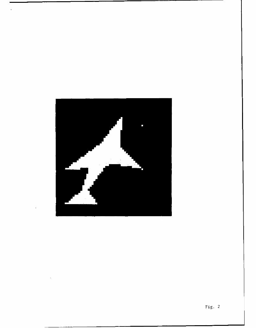
Fig. 2

Fig. 3
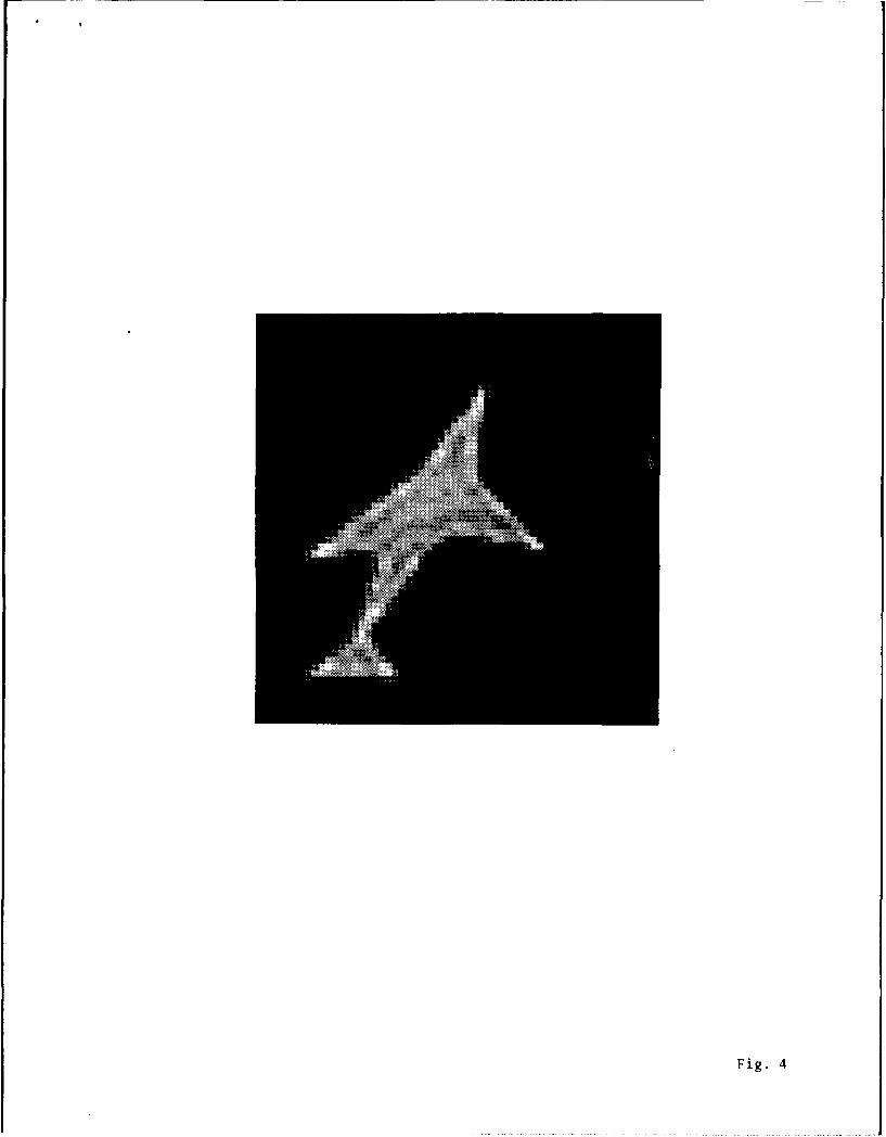
Fig. 4

Fig. 5

Fig. 6
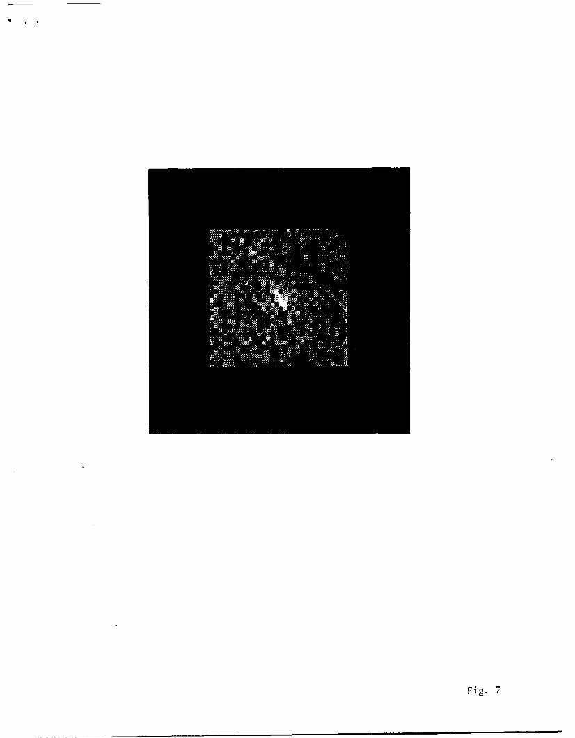
Fig. 7
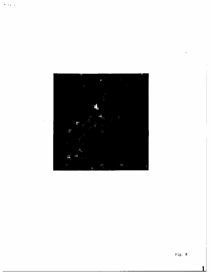
Fig. 8

Fig. 9

Fig. 10
Top Related