

![FLAC [1ex]Turing Machines](https://static.fdocuments.us/doc/165x107/61a8c3af1ccd476a43097a32/flac-1exturing-machines.jpg)


Languages
Pages
Legal

Turing Machines
Wen-Guey Tzeng
Department of Computer Science
National Chiao Tung University
1

Model
2
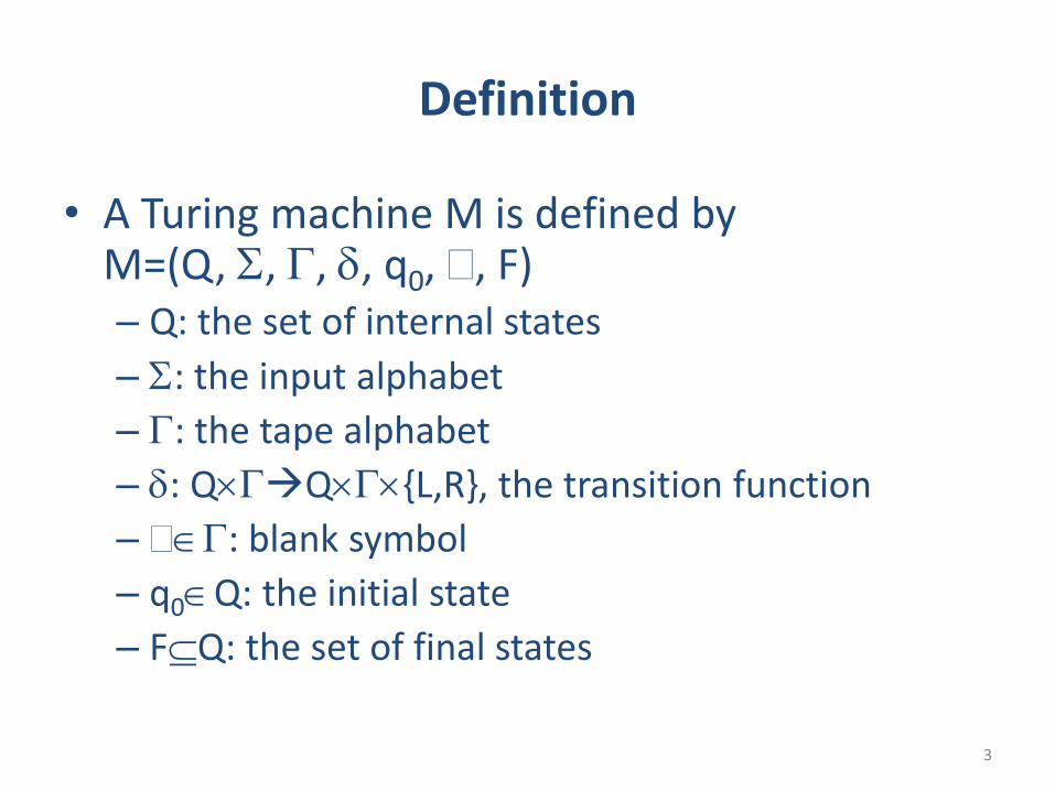
Definition
• A Turing machine M is defined by M=(Q, , , , q0, , F) – Q: the set of internal states
– : the input alphabet
– : the tape alphabet
– : QQ{L,R}, the transition function
– : blank symbol
– q0Q: the initial state
– FQ: the set of final states
3

Transition function
4
• (q0, a)=(q1, d, R)
Example
5
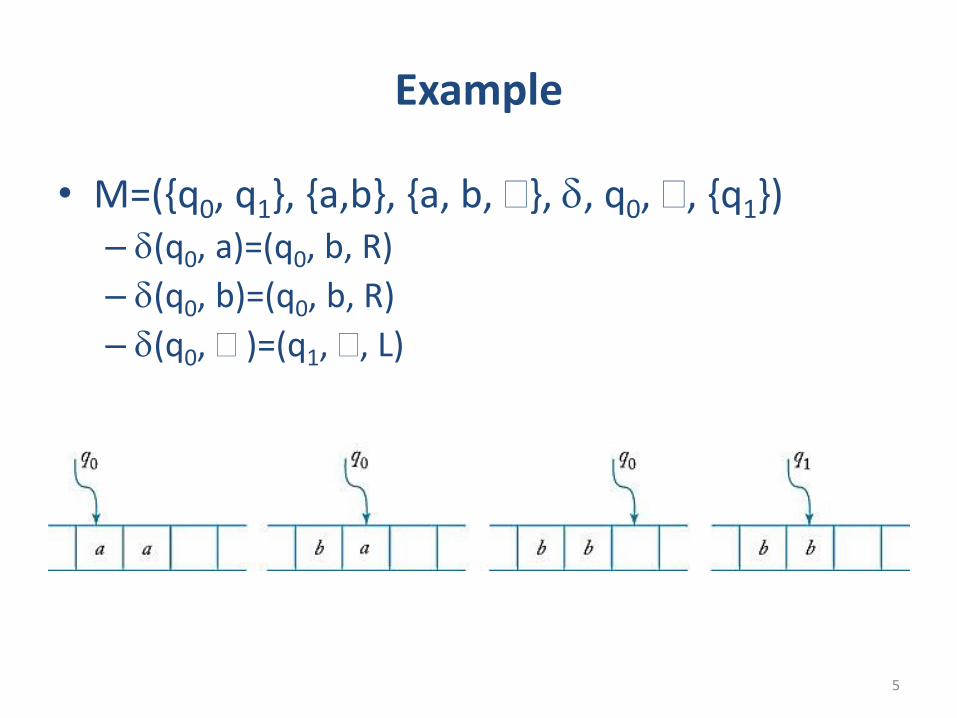
• M=({q0, q1}, {a,b}, {a, b, }, , q0, , {q1}) – (q0, a)=(q0, b, R)
– (q0, b)=(q0, b, R)
– (q0, )=(q1, , L)

Transition graph
6
– (q0, a)=(q0, b, R)
– (q0, b)=(q0, b, R)
– (q0, )=(q1, , L)
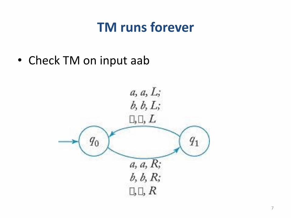
TM runs forever
7
• Check TM on input aab

TM halts
8
• A TM “halts” if it reaches a configuration that is not defined.
– A TM on an input w may not halt. (Run forever)
– The halting of a TM on some input w does not mean w is accepted.

Standard TM
• The tape is unbounded in both directions.
• All other cells are filled with blanks.
• It is deterministic.
• The input is on the tape in the beginning.
• No output devices. But, the left string on the tape can be viewed as output.
9
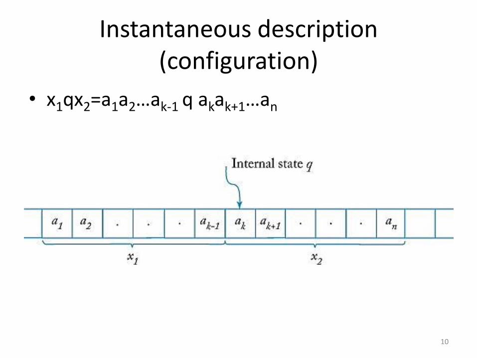
Instantaneous description (configuration)
• x1qx2=a1a2…ak-1 q akak+1…an
10
Example
11
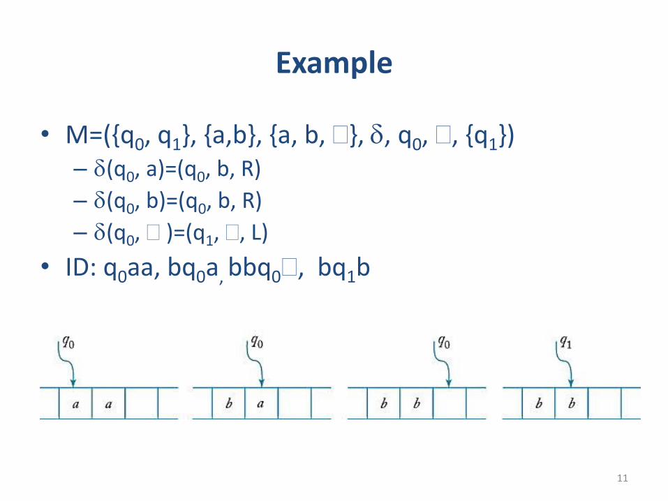
• M=({q0, q1}, {a,b}, {a, b, }, , q0, , {q1}) – (q0, a)=(q0, b, R)
– (q0, b)=(q0, b, R)
– (q0, )=(q1, , L)
• ID: q0aa, bq0a, bbq0, bq1b
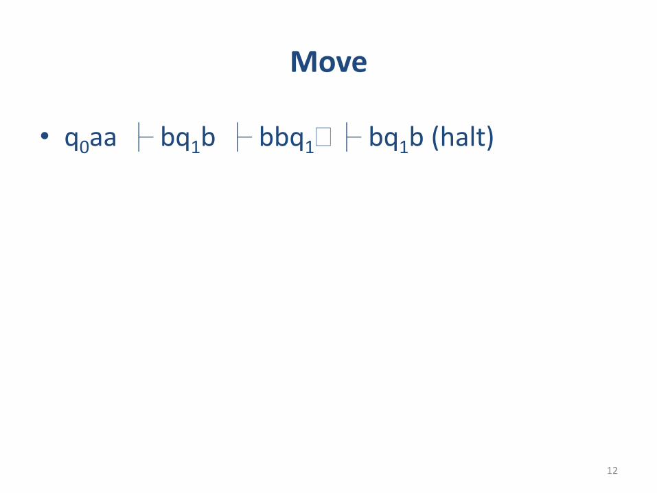
Move
• q0aa ├ bq1b ├ bbq1├ bq1b (halt)
12
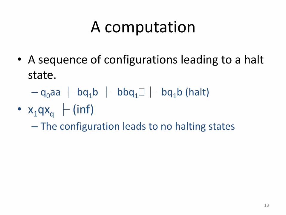
A computation
• A sequence of configurations leading to a halt state.
– q0aa ├ bq1b ├ bbq1├ bq1b (halt)
• x1qxq ├ (inf)
– The configuration leads to no halting states
13
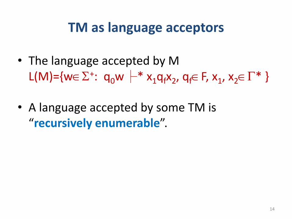
TM as language acceptors
• The language accepted by M L(M)={w+: q0w├* x1qfx2, qfF, x1, x2* }
• A language accepted by some TM is “recursively enumerable”.
14

Example
• Design a TM to accept the strings of form 00*
• The transition function
– (q0, a)=(q0, 0, R)
– (q0, )=(q1, , R)
15

• Design a TM to accept L={anbn : n1}
• Idea:
– Loop
• Mark leftmost ‘a’ as ‘x’ in the tape
• Move all the way right to mark ‘b’ as ‘y’
– After marking all a’s, move all the way right to find
16

• Mark leftmost ‘a’ as ‘x’ in the tape
– (q0, a)=(q1, x, R)
• Move all the way right to mark ‘b’ as ‘y’
– (q1, a)=(q1, a, R)
– (q1, y)=(q1, y, R)
– (q1, b)=(q2, y, L)
17

• Move back to mark leftmost ‘a’ as ‘x’ – (q2, y)=(q2, y, L)
– (q2, a)=(q2, a, L)
– (q2, x)=(q0, x, R)
• After marking all a’s, move all the way right to find – (q0, y)=(q3, y, R)
– (q3, y)=(q3, y, R)
– (q3, )=(q4, , R) – If in the middle ‘b’ is encountered, TM stops.
18

• Run q0aabb
19
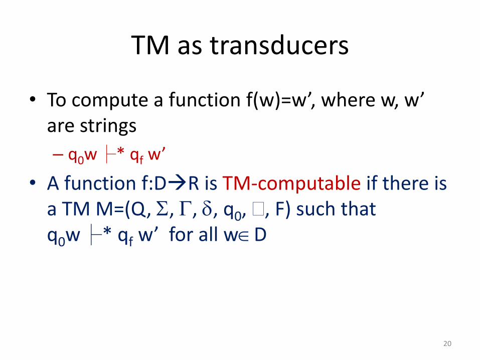
TM as transducers
• To compute a function f(w)=w’, where w, w’ are strings
– q0w├* qf w’
• A function f:DR is TM-computable if there is a TM M=(Q, , , , q0, , F) such that q0w├* qf w’ for all wD
20

Example
• Given two positive integer x and y, compute x+y
– x and y are unary-represented
– Eg. X=3, w(x)=111
– Input: w(x)0w(y)
– Output: w(x+y)0
– That is, q0w(x)0w(y)├qfw(x+y)0
21
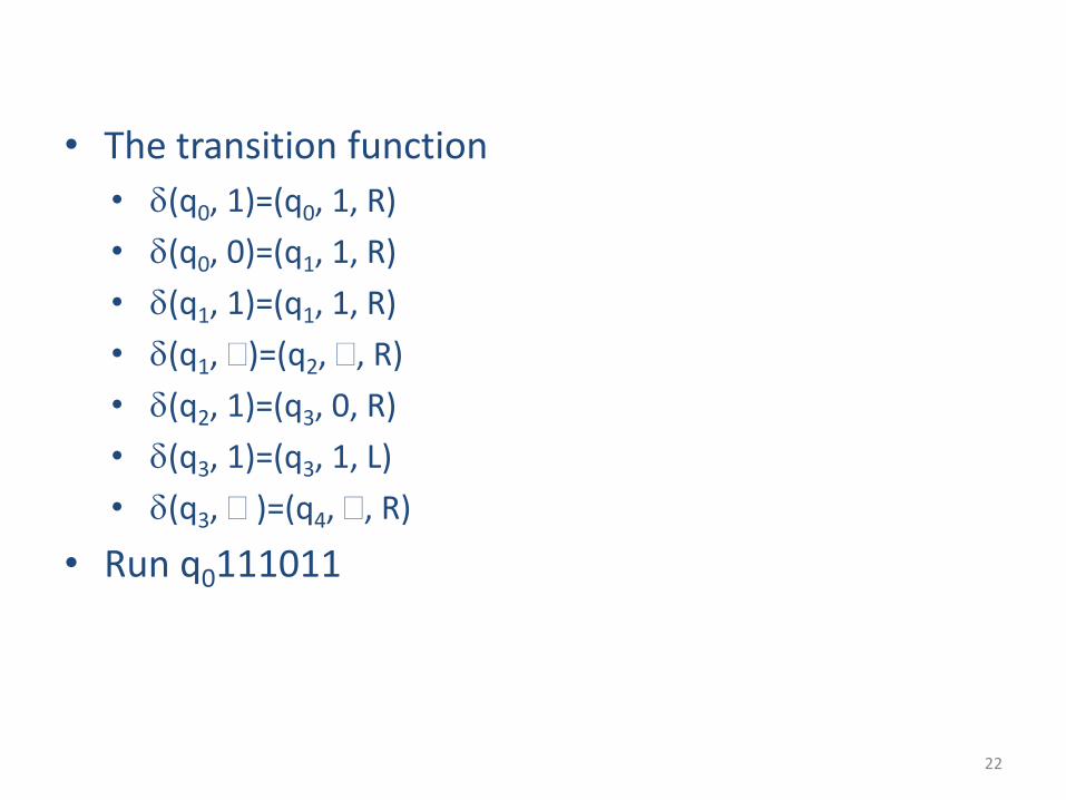
• The transition function
• (q0, 1)=(q0, 1, R)
• (q0, 0)=(q1, 1, R)
• (q1, 1)=(q1, 1, R)
• (q1, )=(q2, , R)
• (q2, 1)=(q3, 0, R)
• (q3, 1)=(q3, 1, L)
• (q3, )=(q4, , R)
• Run q0111011
22
Example
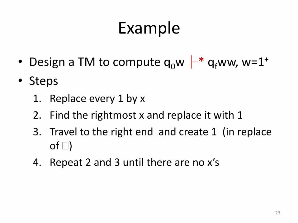
• Design a TM to compute q0w├* qfww, w=1+
• Steps
1. Replace every 1 by x
2. Find the rightmost x and replace it with 1
3. Travel to the right end and create 1 (in replace of )
4. Repeat 2 and 3 until there are no x’s
23

24
Run q011

Example
• Design a TM to compute q0w(x)0w(y)├* qyw(x)0w(y) if xy q0w(x)0w(y)├* qNw(x)0w(y) if x<y
• Design a TM to compute q0w(x)0w(y)├* qfw(xy)
25

Combining TM for complicated tasks
• Design a TM to compute f(x,y)=x+y if xy f(x,y)=0 if x<y
26

• qC,0w(x)0w(y) ├* qA,0w(x)0w(y) if xy ├* qE,0w(x)0w(y) if x<y
• qA,0w(x)0w(y) ├* qA,fw(x+y)0
• qE,0w(x)0w(y) ├* qE,f 0
27
Example
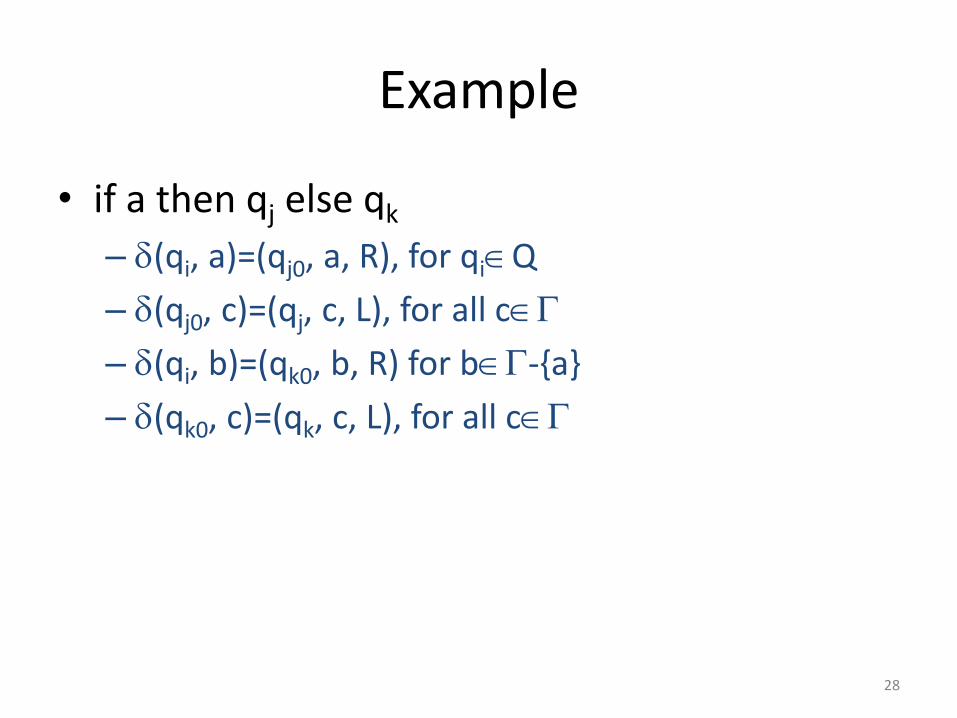
• if a then qj else qk
– (qi, a)=(qj0, a, R), for qiQ
– (qj0, c)=(qj, c, L), for all c
– (qi, b)=(qk0, b, R) for b-{a}
– (qk0, c)=(qk, c, L), for all c
28

Example
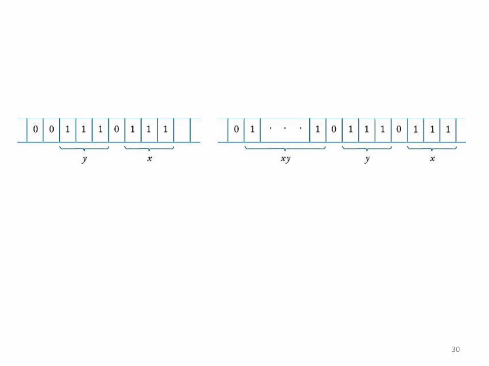
• Design a TM for q0w(x)0w(y)├* qfw(xy)
• Steps
– Loop until x contains no more 1’s
• Find a 1 in x and replace it with another a
• Replace leftmost 0 by 0y
– Replace all a’s with 1’s
29
30

Macroinstructionssubprogram
• A calls B
31

Turing’s Thesis
• Mechanical computation
– Computation without intervention of humans
• Turing Thesis: any computation that can be carried out by mechanical means can be performed by some Turing machine.
• Some call it “Church-Turing Thesis”
32
• Reasoning:
– Anything that can be done by an existing digital computer can be done by a TM
– No one has yet been able to suggest a problem, solvable by algorithms, that cannot be solved by some TM
– Other models are proposed. But, they are no more powerful than TM’s
33
Algorithms
• An algorithm for a functin f:DR is a Turing machine such that q0d├* qff(d) for all dD
34
Top Related