
![[PPT]PowerPoint Presentation - Data Communications … · Web viewCommunication Hub Variant types SW WAN MESH HAN GAS TOSHIBA F7210000 MADE IN CHINA Cellular SW WAN MESH HAN GAS TOSHIBA](https://static.fdocuments.us/doc/165x107/5b8742527f8b9a162d8e9ec7/pptpowerpoint-presentation-data-communications-web-viewcommunication-hub.jpg)


Languages
Pages
Legal


Draft 12.0. Copyright 2009. All rights reserved. 46
4 Mesh Control in SW Simulation
4.1 Introduction
You must plan ahead when building a solid model so that it can be used for realistic finite element load and/or restraint analysis cases. You often do that in the solid modeling phase by using lines or arcs to partition lines, curves, or surfaces. This is called using a “split line” in SolidWorks and SW Simulation. There is also a “split part” feature that is similar except that it cuts a part into multiple sub‐parts. You sometimes need to do that for symmetry or anti‐symmetry finite element analysis so that we can analyze the part more efficiently. Here, the concept of splitting surfaces for mesh control will be illustrated via stress analysis.
4.2 Example Initial Analysis
The split line concepts for mesh control will be illustrated via the first tutorial “Static Analysis of a Part”, using the SW Simulation example file Tutor1.sldprt which is shown in Figure 4‐1. (Remember to save it with a new name by putting your initials at the front.) Consider that tutorial to be a preliminary analysis. You should recall that there was bending of the base plate near the loaded vertical post. However, the original solid mesh had only one element through the thickness in that region and would therefore underestimate the bending stresses there. You need to control the mesh there to form 5 to 6 layers to accurately capture the change in bending stress through the thickness.
Figure 4‐1 Original part, restraints, load, and mesh
The original deformed shape, in Figure 4‐2, is shown relative to the undeformed part (in gray). You see bending at the end of the base and deflection of the part bottom back edge in the direction of the (unseen) supporting object below it. From the original effective stress plot in Figure 4‐3 and Figure 4‐4 you can see that large regions, within the red contours, have exceeded the material yield stress. Actually, the maximum value is over 133,000 psi, or about 1.5 times the yield stress, on the top and bottom of the base. Clearly, this part must have its material or dimensions changed and/or new support options must be utilized.
4.3 Structural Restraint Options in SW Simulation
Solids and shells must be restrained and loaded in different ways since shells also have rotational degrees of freedom and solids do not. Table 4‐1 lists the current restraint or fixture options for solids within SW Simulation. Note that they only involve components of the displacement vectors. The loading options for solids are given in Table 4‐2. They involve only forces, pressures, temperature differences, and accelerations.

FEA Concepts: SW Simulation Overview J.E. Akin
Draft 13.0. Copyright 2009. All rights reserved. 47
No pure couples (moments) can be specified at a node. Of course, loadings statically equivalent to applied couples can be specified by spatially varying pressures.
Once the restraints, loads, and materials have been specified the mesh must be generated, as discussed in the next section. For complicated parts it is sometimes wise to generate the mesh first. The mesh generation phase can fail for various reasons (mainly bad solid models or insufficient memory resources). If it does fail the time spent on loads and restraints may be wasted. When a mesh exists too, you proceed on to running the analysis. Then you must conduct and document the post‐processing the analysis results. Those phases will be introduced in the following general introduction to SW Simulation for stress studies.
Table 4‐1 Fixtures for solid stress analysis Fixture Type Solid Element Definition Fixed or Immovable All three translations are zero on face, edge, or vertex. Hinge On a cylindrical face, only the circumferential displacement is allowed. On cylindrical face The cylindrical coordinate displacements normal to and/or on the
cylindrical surface are given. On flat face Displacements normal to and/or tangent to a flat face are given. On Spherical face The spherical coordinate displacements normal to and/or on the
spherical surface are given. Roller/Sliding or Symmetry Two displacements tangent to a flat face are allowed. Use reference geometry A face, edge, or vertex can translate a specified amount relative to a
reference plane and axis.
Table 4‐2 Load conditions for solid stress analysis Load Type Solid Element Definition Apply force The total force on a face, edge, or vertex is given relative to a single
edge or axis direction. Apply normal force The total force normal to a face, at its centroid, is specified and
converted to an equivalent pressure. Apply torque The total torque on a face is specified with respect to an axis and
converted to an equivalent pressure. Bearing Load On a cylindrical surface give the total force in a Cartesian X or Y direction
to convert to a sine distribution pressure. Centrifugal The angular acceleration and angular velocity are given about an axis,
edge, or cylindrical surface. Connectors See SW Simulation help files. Gravity The gravitation acceleration value is given and oriented by an axis, edge,
or a direction in or normal to a selected plane. Remote load See SW Simulation help files. Temperature Not recommended. Transfer from thermal analysis.
Begin by reconsidering the restraints utilized. In many problems the restraints are unclear or questionable and you need to consider other restraint cases. You previously restrained all the three translations on the two small cylindrical surfaces. That makes those surfaces perfectly rigid. That would be almost impossible to build. It is likely that the holes were intended to be bolt holes. Then the applied backward (‐z) pressure load would probably require the development of tension reaction forces along the back (‐z) half of the bolt cylinder. That would not happen because an air gap would open up. Also, a bolt usually applies a restraint to the surface under the bolt head (in addition to a bolt bearing load on its cylindrical part), and that is not in the original choice of restraints. Furthermore, the bracket seems to be attached to some rigid object under it and

FEA Concepts: SW Simulation Overview J.E. Akin
Draft 13.0. Copyright 2009. All rights reserved. 48
therefore you would expect the back edge of the bracket to be somehow supported by that object when that region of the part deforms as seen in Figure 4‐2. The original effective stresses are in Figure 4‐3 and Figure 4‐4.
Figure 4‐2 Original part vector deflections and bottom right edge graph
Figure 4‐3 Original top surface effectives stresses
As a new possible restraint set, assume that the bolt heads are tight and act on a small surface ring around each hold. That could provide rigid body translation restraints in three directions. Each bolt would prevent three translations and the pair of them combines to also prevent three rigid body rotations. Thus they combine to prevent all six possible rigid body motions (RBM). If the bolts were not tight then only a normal displacement (along the bolt axis) would be restrained on the base top surface (and two RBM would remain).
Bearing loads on the bolt shaft can be found by an iterative process in SW Simulation, but for early studies you can assume a small cylindrical contact at the most positive z (front) location. The previously computed bending of the part is also assumed to cause contact with the supporting object below, and thus a y‐ translational restraint, along the bottom back edge of the part. To accomplish those types of restraint controls you need to “split” the surfaces and transition the mesh in those regions to get better results. Thus, you need to form two smaller surface rings for the bolt heads, and split the cylinders into smaller bearing areas.

FEA Concepts: SW Simulation Overview J.E. Akin
Draft 13.0. Copyright 2009. All rights reserved. 49
Figure 4‐4 Original bottom surface effective stresses
4.4 Splitting a Surface or Curve
To avoid changing the master tutorial file, open the part and then “save as” a new file name on the desktop. To introduce the required split lines:
1. Select the top surface of the base by moving the cursor over it until its boundary turns green and Insert Sketch.
2. Pick the Sketch icon and pick the Circle option to form a bolt head washer area.
3. Place the cursor on the hole edge to “wake up” the center point. Draw a larger circle on the surface. Set its diameter to 30 mm and click OK. That does not change the surface; it just adds a circle to it.

FEA Concepts: SW Simulation Overview J.E. Akin
Draft 13.0. Copyright 2009. All rights reserved. 50
4. To split the surface go to the top menu bar and select Insert Curve Split Line. The Type will be a projection.
5. Next, pick the surface(s) to be cut by this curve. Here it will be the top of the base plate again so select it and click OK. Repeat the above two processes for the second hole.
Now you will see that moving the cursor around shows a new circle and a new ring of surface area that could be used to enforce restraints or loads. The new surface areas are shown in Figure 4‐5. Later you will use these newly created ring areas as a bolt head (washer) restraint region.
Figure 4‐5 The original surface is now three surfaces

FEA Concepts
Draft
To form a ve
1. Selecconst
2. Selecnew
3. Repe
The above suYou will need“L” shaped si
1. Right
2. “Wak
3. Use I
Now youaccount f
s: SW Simula
13.0. Copyri
rtical bearing
ct the top sutruction line f
ct Insert Cload bearing
eat those ope
urface splits wd another suride area to ha
t click on the
ke up” the lef
Insert Curv
u see it has bfor local bend
ation Overview
ght 2009. All
g region on th
urface and usforward from
Curve Splitsurface that
erations for th
were construrface split to ave the leg sp
(+x) right side
ft vertical line
ve Split Line
become two rding.
w
l rights reserv
he bolt hole si
se Sketch m the center, a
t Line and piccould be use
he second bol
ucted to give help exerciseplit off so you
e face, Insert
e to put in a s
e and select t
rectangles. Y
ved.
idewall:
Line. “Wakeand two othe
ck the cylinded to restrain
lt hole.
more flexibile engineering can control a
t Sketch Ske
short vertical
the “L” face, c
You can cont
e up” the cener radial lines
er of the first and/or contr
ity in applying control ovea bending me
etch Line.
line that cros
click OK.
rol the numb
nter point agoffset by abo
bolt hole, clicol the mesh.
ng various disr the revised esh there:
sses the base
ber of layers
J
5
ain. Use it toout 25o.
ck OK. That c
splacement remesh. You w
.
in the smalle
.E. Akin
51
o draw a
creates a
estraints. want the
er one to
FEA Concepts
Draft
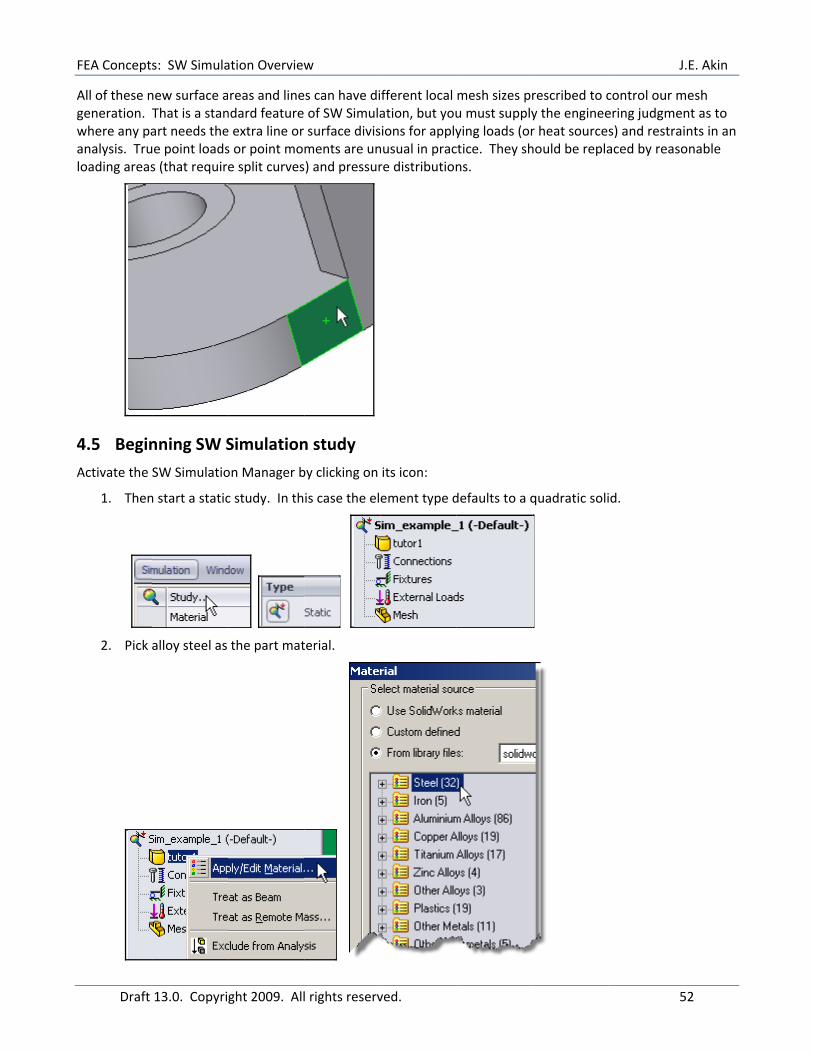
All of these ngeneration. Twhere any paanalysis. Truloading areas
4.5 Begin
Activate the
1. Then
2. Pick
s: SW Simula
13.0. Copyri
new surface aThat is a stanart needs theue point loadss (that require
nning SW S
SW Simulatio
n start a static
alloy steel as
ation Overview
ght 2009. All
reas and linendard featuree extra line or s or point moe split curves
Simulation
on Manager b
c study. In th
the part mat
w
l rights reserv
es can have di of SW Simulasurface divisments are uns) and pressur
n study
by clicking on
is case the el
terial.
ved.
fferent local ation, but yousions for applynusual in pracre distribution
its icon:
ement type d
mesh sizes pru must supplyying loads (orctice. They shns.
defaults to a q
rescribed to cy the engineer heat sourcehould be repla
quadratic soli
J
5
control our mering judgmens) and restraiaced by reaso
id.
.E. Akin
52
mesh nt as to ints in an onable

FEA Concepts: SW Simulation Overview J.E. Akin
Draft 13.0. Copyright 2009. All rights reserved. 53
3. Note that you have a choice of display units for the properties. The number of significant figures in the test data should be independent of the units selected. Any difference is due to using a higher number of digits in the units conversion. Do not be mislead by a long string of digits in materal values. You can usually trust the first three, or maybe four. Note for later use that the yield stress of this material is about 620 MPa or 90 ksi.
4.6 Mesh Control
Wherever translational displacement restraints are applied, reaction forces are developed and localized stress concentrations are likely. Therefore, you want to assure that small elements are created in such regions. This process is referred to as mesh control. It is required in almost every study. Invoke it with:
1. Right click on Mesh Apply Control to bring up the Mesh Control panel. The default element size of about 3 mm needs to be changed in the new regions created above. Select the region around the two bolt washers by picking those two surfaces, and setting the desired size to 1mm.

FEA Concepts: SW Simulation Overview J.E. Akin
Draft 13.0. Copyright 2009. All rights reserved. 54
2. Likewise, for the two bearing surfaces within the smaller vertical cylindrical holes set the size to about
1.0 mm.
3. In the final corner region you need several elements through the thickness of curved front corner to accurately model the local bending seen in the first study. Select the small split rectangle and the adjacent cylindrical corner and use an element size of about 1.5 mm.
FEA Concepts: SW Simulation Overview J.E. Akin
Draft 13.0. Copyright 2009. All rights reserved. 55
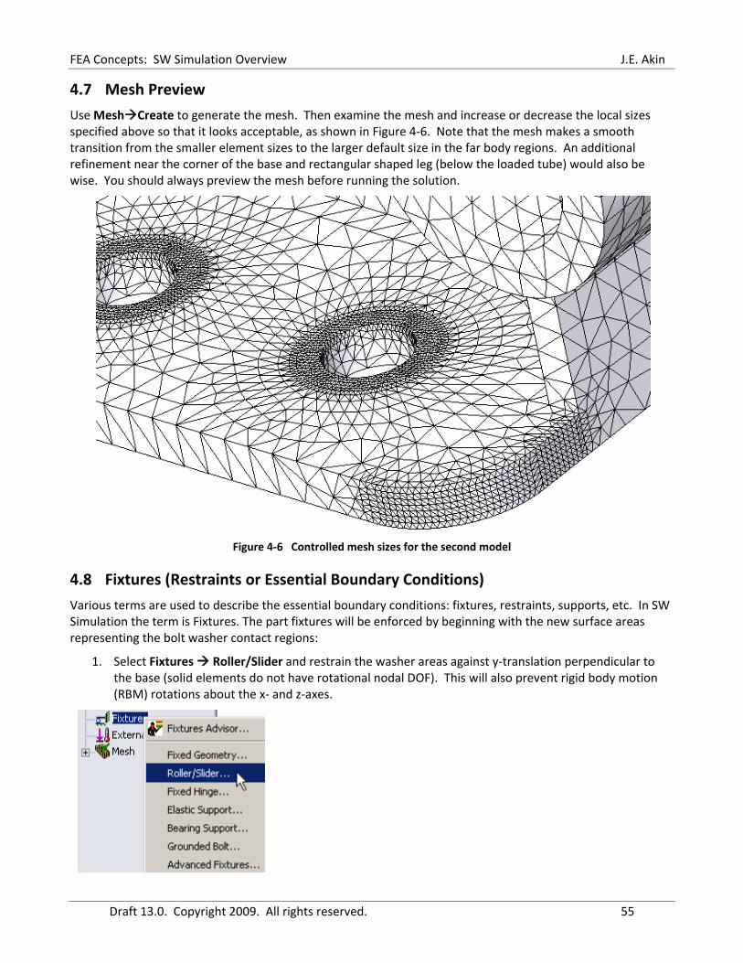
4.7 Mesh Preview
Use Mesh Create to generate the mesh. Then examine the mesh and increase or decrease the local sizes specified above so that it looks acceptable, as shown in Figure 4‐6. Note that the mesh makes a smooth transition from the smaller element sizes to the larger default size in the far body regions. An additional refinement near the corner of the base and rectangular shaped leg (below the loaded tube) would also be wise. You should always preview the mesh before running the solution.
Figure 4‐6 Controlled mesh sizes for the second model
4.8 Fixtures (Restraints or Essential Boundary Conditions)
Various terms are used to describe the essential boundary conditions: fixtures, restraints, supports, etc. In SW Simulation the term is Fixtures. The part fixtures will be enforced by beginning with the new surface areas representing the bolt washer contact regions:
1. Select Fixtures Roller/Slider and restrain the washer areas against y‐translation perpendicular to the base (solid elements do not have rotational nodal DOF). This will also prevent rigid body motion (RBM) rotations about the x‐ and z‐axes.

FEA Concepts: SW Simulation Overview J.E. Akin
Draft 13.0. Copyright 2009. All rights reserved. 56
2. In the Standard panel pick the two concentric ring faces as the Selected Entities and chose Roller/Slider as the Type.
3. Next select the two cylindrical bolt bearing faces and restrain radial translation on the Advanced Fixtures On Cylindrical Faces Type. That prevents x‐ and z‐translational RBM and the y rotational RBM. At least all RBMs are now safely accounted for.
4. Finally, this study will assume the bottom back edge helps support the part due to contact with the strong background material, to which the bolts are also assumed to be rigidly attached. Use Fixtures
Advanced Use Reference Geometry. Select that back edge line and choose the bottom plane as your reference plane Type. Restrain the edge line displacement, relative to the bottom, by picking the vertical direction (perpendicular to the bottom plane) and preview the restraint arrow to verify the correct choice. That prevents RBM in y translation and z rotation.

FEA Concepts: SW Simulation Overview J.E. Akin
Draft 13.0. Copyright 2009. All rights reserved. 57
4.9 Pressure loading
This part has one pressure loading on the large front tube face. Impose it with:
1. External Loads Pressure.
2. In the Pressure panel give the Pressure Type as normal to the selected face, set the units and value (1,000 psi) and preview the arrows to verify the direction (sign of the pressure), OK. At this point, you may wish to take advantage of the standard Windows feature and rename this load condition from the default Pressure_1 to Front_ring_pressure, by doing a slow double click on the default name.

FEA Concepts: SW Simulation Overview J.E. Akin
Draft 13.0. Copyright 2009. All rights reserved. 58
Clearly, the resultant applied force will be that pressure times the selected surface area. Since SolidWorks is a parametric modeler remember that if you change either diameter of the tube the area and the resultant force will also change. If you mean to specific the total force then use External Loads Force and give the total force on that area. It would not change with a parametric area change.
Remember that when the study results are obtained later, to check the total force caused by the above pressure you can check the reaction force since it must be equal and opposite. (You can do that in post‐processing by right clicking on the Displacement report Reactions). The z‐reaction force will give the equal and opposite force to the total applied here (since this is the only z‐force applied in this example).
4.10 Run the Study Right click on the study name and select Run. Proceed to post‐processing the results as shown below.
4.10.1 Check support reaction values After any structural or thermal study you should check the reactions from the surroundings that were approximated as restraints or fixtures. They will be equal and opposite to the resultants of the applied loads or heat sources. Right click on Results List Result Force Reaction force. Under Selection pick the restraint regions in the model, and set the units. Update gives the plot shown (Figure 4‐7), and a table of component values for the forces. (Study the plot as it will be reconsidered later.)

FEA Concepts: SW Simulation Overview J.E. Akin
Draft 13.0. Copyright 2009. All rights reserved. 59
Figure 4‐7 Reaction forces from the washers, bolts, and back edge
The ring of pressure applied in this problem was totally in the z‐direction. Therefore, there should be no reaction forces in the x‐ and y‐directions. While not zero they are times smaller. The iterative solver was used to get the current results. It is much faster than the optional direct solver, but a direct solve will be slightly more accurate. When obtained from a direct solve the reaction forces are more correct (below), but the difference is not important..
4.10.2 Display a design insight Some engineers try to visualize how the major loads are transferred to the supports via the “load path”. SW Simulation has a tool to assist with that: Right click on Results Define Design Insight Plot.
Figure 4‐8 Major material "load path" through the part

FEA Concepts: SW Simulation Overview J.E. Akin
Draft 13.0. Copyright 2009. All rights reserved. 60
4.10.3 Displacement results
Start with the color contour of the part, but with the contours scaled to match those of the previous study: Results Displacements, then Chart Options Display Options Defined and set the prior maximum value. Figure 4‐9 (left) shows the new displacement distribution which is less that half as large as before, and includes smaller regions of bending. To add a more informative displacement vector plot:
1. Right click in the graphics area. Then pick Edit Definition Advanced Options Show as vector plots OK.
2. When the displacement vector plot appears use Vector Plot Options to dynamically control the clarity. Rotate this view (hold down the center mouse button and move the mouse) to find the most informative orientation.
The right side view of the original displacements is shown amplified in Figure 4‐10 (left) and compared on the right to the new displacement values. Both are shown at the same scale, along with the gray undeformed part. As with the first approximation, the main bending region is the rounded front corner of the base plate. The mesh there is now fine enough to describe the flexural stress and shear stress as they change through the thickness. The default contour plot style for viewing the displacements is a continuous color variation. These are pretty and should be used at some point in a written stress analysis report, but they can hide some useful engineering checks.
Figure 4‐9 Alternate restraints significantly reduce peak deflections

FEA Concepts: SW Simulation Overview J.E. Akin
Draft 13.0. Copyright 2009. All rights reserved. 61
Figure 4‐10 Original (left) and revised displacement vectors, to the same scale
4.10.4 Effective (von Mises) stress
The effective stress distribution on the top of the base is shown in Figure 4‐11. There two different contour options are illustrated. The line contour form tends to be more useful if preliminary reports are being prepared on black and white printers. The material yield stress was 90,000 psi, so every region colored in red is above yield. In that figure, the Edit Definition feature was used to manually select the discrete color or line contours. The Chart Options feature was used to specify the stress range and the number of discrete colors. Rotating the part shows that there are other regions of the part above the yield stress. On the bottom corner of the base the assumed line support has also caused high local stresses, as seen in Figure 4‐12. In that figure you should also note that the bottom edge of one bolt bearing surface shows a small region of yielding. That should be examined in more detail and other views.
Line or point restraints are not likely to exist in real part components. You could revise that region by putting in a split line to create a narrow triangular support area. That would be more accurate, if the resulting part stresses there are compressive. Otherwise, you would need to use a contact surface. Using contact surfaces where gaps can develop requires a much more time consuming iterative solution. However, the important thing is to attempt an accurate model of the part response, not an easy model.

FEA Concepts: SW Simulation Overview J.E. Akin
Draft 13.0. Copyright 2009. All rights reserved. 62
Figure 4‐11 Distortional energy failure criterion on the base top surface
Figure 4‐12 Failure criterion in the base bottom region, and back edge
4.10.5 Maximum principal stress
The extreme values of the stress tensor at any point are known as the principal stresses (eigenvalues of the stress tensor). For 3D part, there are three normal principal stresses and a maximum shear stress. The principal normal stress components have both a magnitude and direction. They can be represented as directed line segments with two end arrow heads used to indicate tension or compression. Employ Stress Plot Display P1 Maximum principal stress Advanced Options Show as vector plot. The maximum
principal stress vector plot, at the top of Figure 4‐13, shows the highest tension stress (and is a failure criterion for some materials). Here, it occurs in the yielding region where the base joins the vertical tube support. Those high stress concentrations could (and should) be reduced by adding fillets along the associated edges along the reentrant corners. The color display is from Advanced Options Nodal values.

FEA Concepts: SW Simulation Overview J.E. Akin
Draft 13.0. Copyright 2009. All rights reserved. 63
Figure 4‐13 The maximum principal stress vectors, and magnitude
4.10.6 Failure theory plot The SW Simulation system allows the user to select from a short list of the most studied material failure theories. It can display a plot of a non‐dimensional number representing the value of the theory at every point on the part. A value less than unity means that the selected theory predicts material failure. Many engineers refer to that value as the factor of safety while others refer to it simply as the failure theory factor that is one of many terms, listed in Table 3‐1. To see this type of plot: right click on Results Define Factor Of Safety Plot to open the Factor of Safety panel and in this case select the von Mises criterion, OK. All the factors in that table need to be unity or greater. The resulting plot in Figure 4‐14 shows a minimum material failure theory value of about 0.6. Thus, this design is currently a failure.

FEA Concepts: SW Simulation Overview J.E. Akin
Draft 13.0. Copyright 2009. All rights reserved. 64
Figure 4‐14 Material failure is predicted for the current study
4.10.7 Validate the design revision The reaction results, in Figure 4‐7, suggest an assumption error in this study. In particular, it is important to check the signs of the reactions to verify that they act as you expect. The negative sign of the left bolt reaction in the z‐direction was unexpected. To better illustrate the concern, and to show another post‐processing tool, consider a free body diagram of the regions governing reactions in the z‐direction: right click Results List Force Results Options Free body force. Under Selection set the units and pick the pressure face and the two bolt bearing faces. The forces in the z‐direction are in equilibrium. Consider moment equilibrium about the y‐axis, at the center of the right bolt. The x‐lever arm to the pressure resultant center is 53 mm, while the lever arm to the left bolt is 65 mm. Thus, y‐moment equilibrium is also satisfied (to a 1% round off error). The concern is that the left bolt was assumed to be pushing on the front bearing area. Instead, it is pulling on that area, which is not possible. What is likely is that the bolt is simply pushing on the corresponding area at the back of the hole. The first split line should have been made on the back of the bolt hole. That can be easily fixed. An alternative would have been to include part of the bolts and conduct an iterative contact/gap analysis. That would have take much long (and sometimes fails to converge), but that is often not needed in a preliminary study. The question is, is that support change likely to invalidate the above study results? Looking at the load path sketch of Figure 4‐8 and the stresses in Figure 4‐11 it is unlikely. However, the next study refinement of this part should utilize this information.
FEA Concepts: SW Simulation Overview J.E. Akin
Draft 13.0. Copyright 2009. All rights reserved. 65
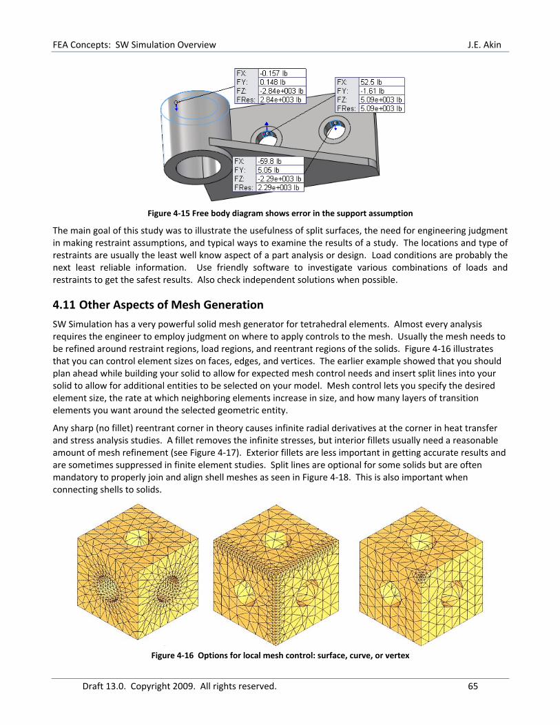
Figure 4‐15 Free body diagram shows error in the support assumption
The main goal of this study was to illustrate the usefulness of split surfaces, the need for engineering judgment in making restraint assumptions, and typical ways to examine the results of a study. The locations and type of restraints are usually the least well know aspect of a part analysis or design. Load conditions are probably the next least reliable information. Use friendly software to investigate various combinations of loads and restraints to get the safest results. Also check independent solutions when possible.
4.11 Other Aspects of Mesh Generation
SW Simulation has a very powerful solid mesh generator for tetrahedral elements. Almost every analysis requires the engineer to employ judgment on where to apply controls to the mesh. Usually the mesh needs to be refined around restraint regions, load regions, and reentrant regions of the solids. Figure 4‐16 illustrates that you can control element sizes on faces, edges, and vertices. The earlier example showed that you should plan ahead while building your solid to allow for expected mesh control needs and insert split lines into your solid to allow for additional entities to be selected on your model. Mesh control lets you specify the desired element size, the rate at which neighboring elements increase in size, and how many layers of transition elements you want around the selected geometric entity.
Any sharp (no fillet) reentrant corner in theory causes infinite radial derivatives at the corner in heat transfer and stress analysis studies. A fillet removes the infinite stresses, but interior fillets usually need a reasonable amount of mesh refinement (see Figure 4‐17). Exterior fillets are less important in getting accurate results and are sometimes suppressed in finite element studies. Split lines are optional for some solids but are often mandatory to properly join and align shell meshes as seen in Figure 4‐18. This is also important when connecting shells to solids.
Figure 4‐16 Options for local mesh control: surface, curve, or vertex

FEA Concepts: SW Simulation Overview J.E. Akin
Draft 13.0. Copyright 2009. All rights reserved. 66
Figure 4‐17 Avoid a small number of elements (left) along arcs or through the thickness
Figure 4‐18 Split lines give you more mesh control
Bad solid modeling practices are probably the most common cause of failure of the mesh generation. The mesh generator begins with the edges of a solid. It divides them into segments corresponding to the requested element sizes. However, if the mesh generator encounters a line segment that is smaller than the requested element size, then it must decrease the minimum element size the match the short line. After processing the boundary lines, the generator proceeds to the part surfaces. Then it fills those faces with triangles of the minimum to the requested size. From the triangles (initial solid element faces) it proceeds inward to fill the volume with tetrahedrons. If the edge lines are much smaller that the requested element size (Figure 4‐19), or if they join at very small angles then the mesh generator tries to use tiny elements to match the poor local part geometry. If it is possible to do that the mesh is still likely to fail due to insufficient computer memory. Part flaws are often too small to see without zooming in on the part.

FEA Concepts: SW Simulation Overview J.E. Akin
Draft 13.0. Copyright 2009. All rights reserved. 67
Figure 4‐19 Bad solid models cause meshing failures
Top Related