
![REIF - Duke Universityreif/paper/storer/minturn.pdf · Reif and Storer [16] have considered the problem of 183 computing paths of minimal length in two- and three- dimensional Euclidean](https://static.fdocuments.us/doc/165x107/5b6f78707f8b9a73618c4dbf/reif-duke-university-reifpaperstorer-reif-and-storer-16-have-considered.jpg)


![A Proposed Probabilistic Extension of the Halpern and ... · been proposed by Halpern ([2008], pp. 200–5), Halpern and Hitchcock ([2010], pp. 389–94, 400–3), and Halpern and](https://static.fdocuments.us/doc/165x107/6057db13fe4a5562be12ee7a/a-proposed-probabilistic-extension-of-the-halpern-and-been-proposed-by-halpern.jpg)

Languages
Pages
Legal

128 .I. E Halpern, J. H, Reif
are deterministic. Indeed, historically, much of the research in logics of programs
had dealt only with deterministic programs (cf. the work of Salwicki and his
coworkers in Algorithmic Logic, e.g., [27, 181). One way of excluding nondetermin- ism from PDL is to give the primitive programs deterministic semantics, and then
restricting the use of * and u so that they only occur in contexts which yield
deterministic, well-structured programs. This gives us programs equivalent to those
built up from the atomic programs using the constructs
while. . . do. . . od and if. . . then. . . else. . . fi.
Strict Deterministic PDL (SDPDL) is the restriction of PDL to formulas where
programs are of this sort. Two natural questions arise: (1) Does this restriction to deterministic programs
give US an easier decision procedure. (2) Does it lead to a loss of expressive power.
i.e.. are there notions which we can express in PDL which are not expressible in
SDPDL? The answer to both questions turns out to be “yes”. (The latter result
ans*sers an open question of Hare1 [ 121.) In fact we show that the problem of
deciding SDPDL satisfiability is complete for polynomial space (cf. Theorems 5.1 and 6.3). This result is also shown to hold for other logics of programs. such as
linear time temporal logic (cf. [8,22,29]).
Both the algorithm and expressibility results are based on structure theorems for
m<>dels of SDPDL formulas which show that if a formula p :., satisfiable. it is
satisfiable in a tree model with only polynomial& many nodes at each depth. In
fact, given any tree model for p, we show that we can always find a sub,trt‘e with
only polynomially many nodes at each depth which ih also a model of p (cf. Theorems 4.12 and 3.21).
These proofs give us insight into the effects of nondeterminism on intractabilit>
and expressiveness in program logics. Essentially they show that a dete- ninistic
(SDPDL) program cannot examine every node of a full binary treL. while a
rtondet~rministic program can. This situation has been &own to hold even in the first order case (cf. [ 1 I), 41). Thus first order regular dynamic logic can be shown to
be more expressive than its deterministic counterpart, answering another open
question of Hare1 [ 121 (cf. [ 171. which studies the quantifier-free case). By contrast.
Meyer and Tiuryn [ 16) have shown that I~ondeternlinist~~ does not lead to more expressive power in the case of first order dynamic logic with recursively enumerable
programs. since a deterministic r.e. program can do a breadth-l-irst search of a tree.
Kcsultc sin~ililr to our Theorems 5.1 and 3.2 on polynomial space completeness
have been announced independenOy by Chlebus [5].
The rest of the paper is organized as follo\vs. We review the syntax iind semantics
of PDL in Section 2, and introduce the modifications nwcssa~y to gef SDPDL. Section 3 recalls the basic notions of the Fischer-Lrldntr closure and tab,leaux, which
have proved very useful in obtaining results ahour PDL, and gives the modifications
of these notions appropriate to SDPDL. In Section 4 we introduce free rwdels and twk nzodels. and prove a number of technical result> about them which we wili
need for our decision procedure and expressiveness results. In Section 5 we give a
procedure for deciding if an SDPDL formula is satisfiable which runs in polynomial
space and show that the decision problem is polynomial space hard. 1.~ Section 6
we show that SDPDL is less expressive than PDL. Finally, in Section 7 we give a
complete axiomatization of SDPDL.
2. Syntax and semantics
SDPDL is in fact a restriction of Deterministic PDL (DPDL), the logical theory
with the same svntax as PDL but its semantics restricted so that ill ear!: c;tate an
atomic program-specifies at most one successor state. DPDL. like PDL, is known
to have a decision procedure which is complete in exponential time (cf. Cl],. We
briefly review the syntax and semantics of PDL and DPDL.
2.1. Syntax. The alphabet for PDL (as well as DPDL). K consists of a set @,,.
whose elements are called atomic formulas. a set Z,,. whose ekments are called
atomic programs. and the special tokens U. :, *, '?. I, (. ). (. ) and trrre.
The set of programs, X. and the set of formulas, 0, are defined inductively using the fol towing rules:
Rdt* I. An! atomic program in I,, is a program.
Rdv 2. If (I and b are progr;uns. then so are I a : h), (a u b) and [I:‘: !w will occasionally omit the parent hews).
Ruk 3. Any atomic formula in @,, is a formula; true is a formula.
Rdt~ 4. lf p is ;i formula and LI is a program. then -1~ and (cI)~ (pronounced
‘dktmond (1 p’b arc formulas.
2.2. Notation, WC will normally reserve I’, 0, R. . . . for members of @,,. arid A,
Il. c . . . for JllCJll tWS of Is‘,,. ‘I-hc kttcrs 1’. q. I: . . . denote formulas, while the letters
14. b, t*. . . . dtxiotc programs.
2.3. Definition. A tWt_ strlwtwe ,I! i\ a triple ( Stl, JT-\~, gll ) where S,zr is a set whose
elements are c:llled states. qI : (D + iP( S,, ) is an assignment of formulas to sets of
states and P\~ : z + .ip( S,, x S,, ) is a mapping of programs into binary relations on
S,, \vhjch sntjsfies the folltrkvjng constraints (we omit the subscript M here and
I 30 J. Y. Halpern, J. H. Re[f
elsewhere in the paper if the structure is clear from the context):
(1) 7r(itrue) = 63,
(2) 4 p) n rbp) = ti,
(3) P(a ; 6) = pW”p(~) (composition of relations),
(4) pmJ~~=pw~pw (union of relations),
(5) p(a*) = (p(a))* = IJ,, _(, p( u”) (reflexive and transitive closure)
(where a0 = true?, and u” = a ; n l . ; n, n times),
(6;) p!p?)=Ib, @I= fl(y)). A DPDL structure satisfies in addition:
(7) For all A E &), p(A) defines a partial function,
i.e., it (s, t), (s, t’) E p(A), then I = t’.
If PE @, then we can view r(p) as the set of states in which p is true. And if
N C: 2. then p(a) is the input-output relation of program c(, i.e., (X 14 E p(a) means
that by starting in state II and running program Q we can halt in state c. The size of a structure 144 = (S, T, p) is the cardinality of S.
(4) I=~,>, p (p is (D)fDL &id) iff for ail (D)PDL models A4 = (S, 7~, p) and all
SES, we have M, sb=p.
Note that p is valid iff --up is not satisfiable.
2.7. SDPDL. Now we are ready to define SDPDL. We would like to guarantee
that the only programs which appear illside boxes and diamonds are deterministic
ones. We do this by defining the set of SDPDL programs, &, to be simply the
DPDL programs in which u and * appear only in constructs of the form ((p? ; a) u (lp?; h)) and ((p?: a); lp?), which we abbreviate to if p then a else h fi and while p do a od respectively. This restricted class of programs clearly corresponds to the
well-known while programs. The SDPDL formulas, @,. are those formulas of @
involving only programs of Z,. The semantics of SDPDL is the same as that of DPDL.
For pr @,. let IpI, be the length of p measured as a string over
di,, u &, u {if, then, else. fi. while. do. od. (. ). (, ). ;}.
We omit the subscript s in /pj\ when it is clear from context.
The following two lemmas describe the basic relationships among the programs
and formulas of 2‘, and @,. While the proofs are trivial. the results v.41 be used
throughout this paper and the reader -hould understand them thoroughly before
soing on.
Proof. Parts ( 1 1 and (2) arc immeJi:~tr: from [)etinitio~s 2.3 arid 2.7. Part (3) follows
frilly part\ f 1 1 and (2) by induction on the structurl: of progr;‘ms. We omit details. T-2
1.72 .I. Y. Halpern, .I. H. Reif
(8) !===l(wh’l I e p do ~1 od)9 = ((1~ A -79) v ( p A -$a)(while p do n)q)). (9) t--1( p‘?)9 = (1p v 19).
t w i=W(p v cj) = wop v (49). (11) ~(a~(pAq~~((a~pA(a)q). (12) i== 1-!p=p. (13) If “p= 9, then i==(u)p= (u)q.
Proof. The proof immediately follows from the definitions and Lemma 2.8( 3). Note
that the fact that p(u) defines a partial function for all a E & is crucial to the proof of parts (5) and (11). These are not valid formulas of DPDL. II
In what follows we always assume, unless explicitly stated otherwise, that all
programs and formulas are in 1, and ~0, respectively.
2.10. Depth of testing. Let DPDL,, be 41 the DPDL formulas with no occurrences
of wxs (programs of the form p?). Let DPDL, 1 I be those DPDL formulas where.
if p? occurs as a program in the formula, 11 E DPDL,. Note that DPDL = IJ, DPDL,.
Let SDlWL~, = DPDLj n SDPDL. Thus, for example, we have
((((q‘?;A)“; -1q?)17)‘.);Ru(7((~~:);A)~‘:- ly‘?)f,)‘~;(“;rrlre~ = (if (while 9 do A ad)/) then B else C fi)tntc E SDPl>L>. _
3. FL,-closures and tableaus
Propositional dynamic logic 133
(2) ta ; b)q E F --, (u)(b)q E F,
(3) (if p then a else b fi)q E F + lp, p. (a)q, (b)q E F, (4) (while p do a od)q E F + up, p, (a)(while p do a od)q E F,
(5) (p?)qEF --* PEF. (6) T~EF-,~EF.
Define FL,{ p,,) = F u TF (where 1F = (lq 1 q E F}).
3.2. Lemma. 1 lp,,l, = 12. tl2et2 ]FL,( p,,)l s 2n.
Proof. A slight modification of the proof of 17. Lemma 3.2] shows IFi s 11. The
result easily follows. Cl
3.3. Definition. A tablecl~ for p,, is a DPDL structure M = (S. 7, p) such that
?r( p,,) P 0 and for all s E S the following conditions hold for all formulas:
(1) Ms~11p + A4 sbp. (2) 1’vi’. +((a: b)q + A4 s+)(b)q. ( 3) M. s F (if p then a else h fi>q
+[(ifI. SOP alrd ,%I. SF(C~)~) or (A{. .~klp and M. st(b)q)].
W .!I. s t= (while p dq a od)q + [( ,Vf. s k p and M, s I= (a)(while p do a od)q) or ( *Cf. se ip and 34. s != q j].
(5) .%I, 5 L= ( p?)q + (Af. s~=p and M, .+ q).
((4 l . s==7(u:h)q + !vl. s~1(ll)(hbq.
!71 .U. se -(if p then LI else h fi)q + [(M, s I= p and ./I. se -l(cl)cl) or ( M, s F -1p and AI, s i= I( b)q) J,
(SI .I% s t= T(while p do II od)q -+[(M.s~ lpandbf.sk lq)or
( M. s t= p and 34. s I-= -l(a)(while p do a od)q )I. (‘I,) 421. s= -J( p?>q + (;)I!. S!=l/I OJ ,%/I, Sbll/!,
(I(,) .\1. s b (A>q + 3 ((s.I)c p(A) and A4 C==q),
(Hi .\I. s t- 7(,4jq 3 vt ((s, f)c ,,(A, 3 %I, It=-xj),
(13 .iI, s b (while p do (I od)q
Proof. The kst half of the lemma immediately follows from the definitions. For the second half we need the following lemma.
13-I J. Y. Hnlpern, J. H. Ret/
3.4.1. Sublemma. Let M = (S, T, p) be a tableau for po, and (a)pE FL,( p,,). Then
(a) if M, s I= (a)py then 3t ((s, t) E p(a) and M, t t= p),
b) if M, s I= l(a)p, then Vt ((s, t)E p(a)+ M, t I= 1~).
Prroof. We proceed by induction on the structure of programs. The only case which presents any complications is M, s@ l(while p do a od)q. Suppose, in order to obtain a contradiction, that 3 t ((s, t) E p(while p do a od) and M, t /=- 4). By Lemma 2.8 there exist s,,, sI, . . . , sk with so = s, sk = t, such that, for all i < k, (M, si I= p and (s,.. s, + ,) E p(a)) and R/I, pk I= lp. It is easy to show by induction on i, using Definition X3(8) and the main induction assumption, that M, si I= l(while p do a cd)q for all i c k. But this leads to a contradictton since M, sk != 1p and M, sk + 9. q
Proof of Lemma 3.4 (mhued). Returning to the proof of Lemma 3.4, wppose
M = (S. 7~. p) is a t&leau for p,,. Let n”= v I@,,, p”= p 1 E,, and extend them to mappings 7~‘: @, + P(S) and p’: C, + .jP(S X S) so that the model constraints are
satisfied. Let M’ = (S, T’, p’). Then we can show by induction on the size of formula
p and program a, using Sublemma 3.4. I, that
(1) if (n)q~-FL,(p,,). then (s,t)~p(a)4(s,t)~p’(cl).
(2) if (cl)q~FL,(pJand M,sl= 1(a)9,then(s,fkp(aM(s, t)rp’(a),
(3) if lpc: FL,(p,,), then h/l, sk= p-+ M’, SFI), and A/I, sk lp+ ;\I’. sb -1p.
Thus it follows that M’ is a model for p,, whose graph is isomorphic to that of .\I. Z
4. Tree models
Proposirional dynamic logic 13s
.
.
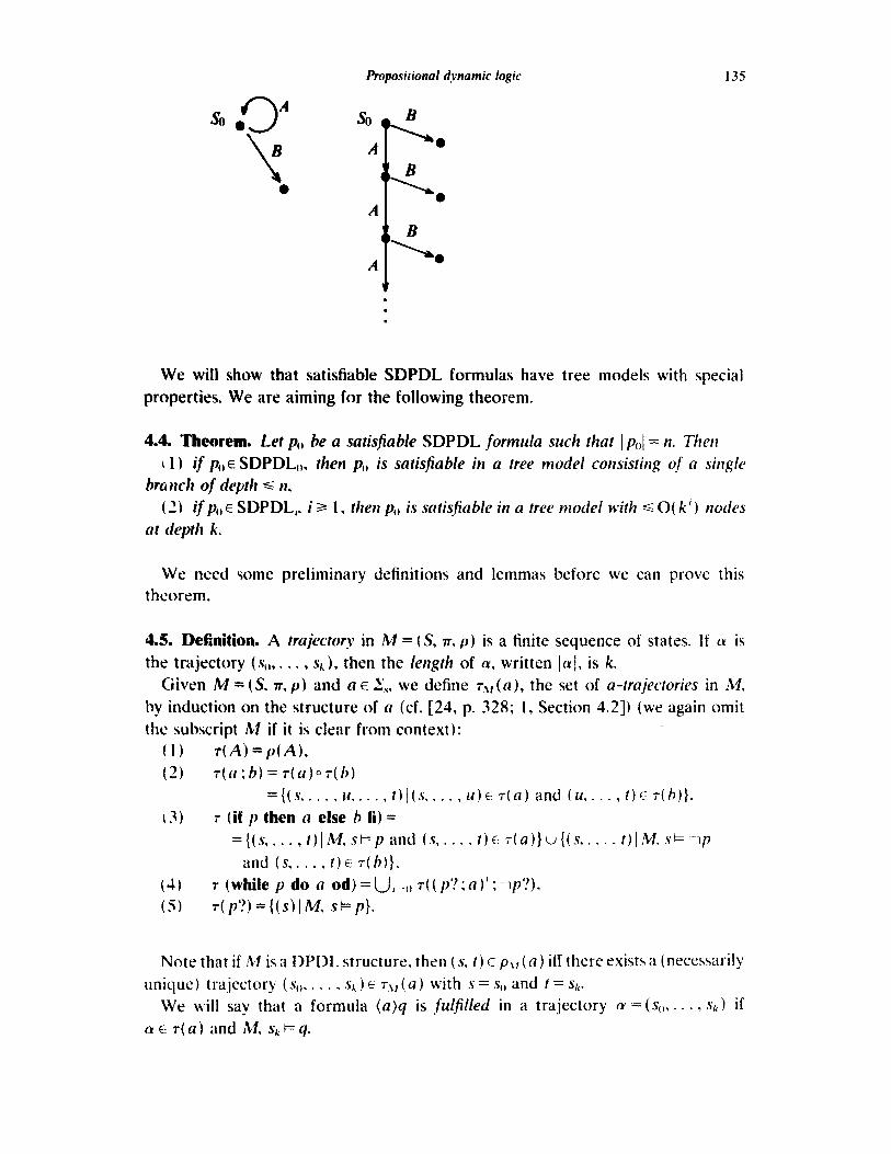
We will show that satisfiable SDPDL formulas have tree models with special
properties. We are aiming for the following theorem.
4.4. Theorem. Let p,, be a satisfiable SDPDL formula such that 1 p(,I = n. Their
t 1) if p. E SDPDL,,, then p,, is satisfiable in a tree model consisting of a sirlgle
branch of depth s n, (3 if p,,E SDPDL,. i 2 1, then p,, is satisfiable in a tree model with s Q( k’) nodes
at depth k.
We need some preliminary definitions and lemmas before we can prove this t hcorem.
4.5. Definition. A trajectory in M = (S, n, p) is a finite sequence of states. If 1x is
the trajectory (so,. . . , sk), then the length of cy, written 1~~1, is k.
Given M=(S, ~,p) and aE:,V,, we define r,,,(a), the set of a-trajectories in M,
by induction on the structure of a (cf. [24, p. 328; I, Section 4.21). (we again omit
the subscript Jb,I if it is clear from context):
(1) r(A)=p(A),
(2) ~(11: b) = 7( a)v( h) ={(s,. . . , u,. . . , t)l(s,. . . , 14)~ T(a) and (~4%. . . , t)c I}.
(2) T (if p then a else b fi) = ={(s,. . . . t)lM, SQJ and (s,. . . . t)c T(a)}u{(s.. . . , t)lM.sb--117
and (s,. . . , t)c r(h)},
W T (while p do a od) = U, .() T( ( p? ; a 1’ ;-y‘?),
(9 T( p’?)={(s)1 M, s+I}.
Note that if M is a DPDL structure, then (s. t) E p.jf (a) itf there exists a (necessarily
unique) trajectory (so, . . . , s,,) E Q (a) with s = s,, and t = sk.
We will say that a formula (a)q is f~#illed in a trajectory cy = (s,,, . . . , sk) if

1 36 .I. Y. Halpern, .I. H. Re(f
4.6. Definition. A straight fine path is a (possibly infinite} straight line graph with
each edge labelled by a primitive program and each node labelled by a finite (possibly
empty) subset of @,.
For typographical reasons we use the notation (II,), A,,, n,, A I, . . .) for a straight
line graph, where IZ, c CD, and A, E I,,. Let g and h be straight line graphs, with g
finite; say g = Cq,, A,), /I~, Al,. . . , AL Ir nk) and It = (HI,,, f?(,, YIP,. . J. Then oh, the concatenation of g and II is the straight line graph
i.e., WC place the graph of tz at the end of g, fusing the first node of h and the last
node of g The lengflz of g, written I,& is k. (For an infinite straight line path f we
say IfI = C) For a node labelled IZ, we define 111,l = E,,, ,I, IpI.
Let f. and A4 he sets of straight line paths. Then. in analogy to regular languages, we CNI define the operations of union. concatenation. Kleene star, and esponenti-
ation on these sets, as follows:
(9 LuM=(glgCx or REM}.
\2) L - ,%I = { gh 1 g E L, II f !kl, and g is finite}.
(‘3) L* ={(O)}u cu, ., L’), (4 L”’ ={gl$ = g,g:,g; * - l pk. g, c L, for all i < k. jgIj K X. itnd I~kl = s)
CJ k/s “SlcE.!ST ’ * * for ;111 i. g, c- I_ and /g,/ q S}
(ix., the dmcnts of L”’ ill-c iIll of infinite knpth. ;1nd consist elf cithu 3 finite cor~c~&matic~n of Amcnt~. of L of which the I;tht li;is infinite length. or i\Il infinitr\
~0 kxtmttion of t’kmnts of L.)
straight line paths, trajectori~vc, alid + .- % fiable formulas. intuitively, a formula p is
satisfiable in a state s iff her:- is a sini +K : iiaight line path in I.,, which is a witness
to this. The straight line paths in I),, ip SOme sense contain the minimal constraints
which have to be met in a model for p These notions are made more precise in
Lemmas 4.0 arid 4.10 below.
4.8. Definition. The straight line path g = ( ao, A,,, ~q, . . . , AL - 1, 1~) and the trajec- tory a = ( sI1. sll . . .) are cmsisteru in M = (S, zr, p) iff Ial = lgl and, for all i < lgl,
( sr,, s,, I) E p(A,), and. for all id Ig’. if pi /I,, then JU s, I= p.
4.9. Lemma. Let .kI = (S, n’. p) be Q DPDL structure.
(21) (so, . . . . sk ) E r(n) iff there is a straight line path in L,, coruistent with
( .$#. . . . , .Q ).
(1~) If M is art SDPDL ruociei. tltert h/l, S,J= p if there is o ( possibly infinite)
trajwtory irl ,$I startirtg with s,, which is consistent with some straight line ptrth it) L,,.
This trajec?q is wkyue. i.e., if ,%I. s,$= p, thati there is exactly orle trajcctw_v in 111
startirq with s,, which is cortsisteitt with some straight lirte path in L,,
Proof. Part (a) follows by a straightforward induction on the structure of programs. Wt: outline the stc‘ps needed to prove part (b):
ti) Using part (a). show that if the statement holds for the formula p, then it
also holds for (a)p.
(ii) By induction on the structure of programs, sho\v that the statement holds
for --l(a)true. As usual, the only case that presents any difficulty is that of l(while p
do LI odhre. Note th:rt AI. sb -$n)trrre iff there is no t with (s, t) E p(a) iff there is
no tr-trajectory starting with s. !Uoreover, it is easy to show there is no t with
(s. t 1 L p(while p do u od\ itf for al! k there is a state tL with (s. tk J E p((p’?; (1 jx ) 01
there is a k and htatc tk with ts, fh) E p((p’?;a)’ ;p‘?) and no a-trajectory starting
with t,,, i.e., tx I= -$&we. Using the iniiuction hypothesis it follows that this is true
iff there is a unique frajector! 3 xting Gth s which is consistent with some straight
line path in
(iii) Now we prove (h) hy induction on the size of p It is trivial if p is an atomic
formula or its negation. If p is of the form (u)q, the result follows from part (i) by
the inductron hypothesk II’ /) is of the form ---q, since M, s I== -1-q iff A4, 3 I= q and
l- q = f.,,, the result again follows from the induction hypothesis. Finally, if p=
-l(a)g, WC have hl, s I= I( o)q iff ( M, s !== (n>-~q or M, s I= l(a)true) iff there is an a-trajectory starting with s consistent with a Krrtiisht line path in L/,‘,) .LI 1.~ L ~\CI ,Irlrc 7
t-y (i), (ii) and the induction hypothesis. Then we are done since L(,,, ,‘, u L icCr)lrL(f’ = I L. _, by Definitiorl 4.7i9i. Z

138 J. Y. Halpern, J. H. Rcif
(a) if p E SDPDLo, then Igl< 1 pi, and, for j< lgl, nj = 8, while nlRl = {q}, where q is of the form P, I P, true, false, or l(A)true, and P E FL,( p),
(b) if pESDPDLi,,, then, for j < 191, nj E SDPDLi n FL,( p) while if Igl C 00,
nl,l E SDPDLi n FLJ p) u {l(A)true 1 A E E,,}).
Moreover, if n, is consistent in the sense that we do not have (4, Tq) c ni for some 4. then I n,l d IpI.
(Intuitively, given a path g = ( nt,, A(,, nl, . . .) E L,, the formulas contained in n,
for j c’ Ig[ are those forced to be there due to tests contained in p I’:;Cus, if p E SDPDL(,,
the 11, will all be empty, while if p is of test depth i+ 1, al\ the brmulas in II, will be of depth 5 i.)
Proof. The idea is to first prove analogous results for programs by induction on structure, and then prove it for formulas by induction on size. We leave the details to the reader. Note that we need the condition in (b) that II, is consistent to deal with such progtxms as while q do P? od. It is easy to see that ({q. -q, P}) E 1 -while q do I’? ody and if 141 is too large we would have (lql+llql+lPIb Iwhile q do P‘? od!. However, (4, --xi, P} is inconsistent, so this example does not
contradict our result. G
Proposirional dynamic logic 139
Proof. Suppose PEE SDPDLi. By Lemma 4.9(b) there is a trajectory in M starting
at so consistent with some g E Ln,, where g = ( no, Ao, nl , Al, . . .) (a) Let i =O. Then, by Lemma 4.10(a), Igl e n. Let (so,. . . , sk) be the trajectory
consistent with g. Note that we have k < n. Let S’ = (~~I,. . . , sk), and let M’ be the
subtree of M determined by S’. Then it follows from Lemma 4.10(a) that the
trajectory (so,. . . , sk) in M' is still consistent with g. Thus, by Lemma 4.9(b),
M', soi= p(,. Moreover, the preceding still holds for any N such that M’s IV s M. Thus M’ sets p,, at SC,.
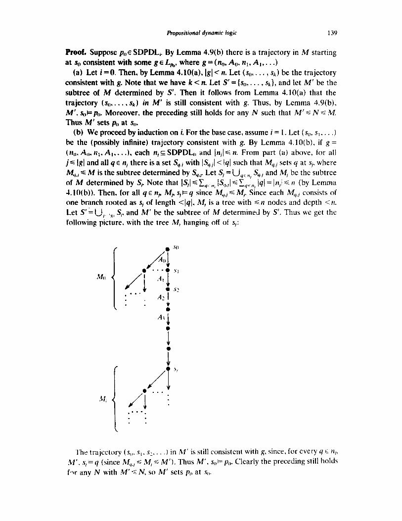
(b) We proceed by induction on i. For the base case, assume i = I. Let ( so, si, . . .)
be the (possibly infinite) trajectory consistent with g. By Lemma 4.10( b), if g =
( )to, A,. 111, A I,. . J, each n,~ SDPDL,, and Ijrjls n. From part (a) above, for all
is 1~1 and all 4 E II, there is a set Sl1.j with ISq.jI < 141 such that Mq.j sets q at sfi where
Ma,, s M is the subtree determined by Sy.l. Let S, = IJ,, n, Sq.j and Mj be the subtree
of k determined by So Note that IS,1 s 1,. ,,, IS‘,,,1 d xllc ,1 jql = In,! s 11 (by Lemma
-I. IO(b)). Then, for all 4 E jrjv Mfi S, k 4 since My-j s M,. Skrce each Mq,J consists of one branch rooted as s, of length ~191, Af, is a tree with s n nodes and depth <II.
Let S' AU, ,s, S,, and M’ be the subtree of M determined by S’. Thus we get the
following picture. with the tree M, hanging off of s,:
J . . * .
The trajectory (s,,, s,, s:, . . . ) in M’ is still consistent with g, since, for every q E ni,
M ‘. s, I= q (since M,,., 6 M, 6 M’). Thus M ‘, s& po. Clearly the preceding still holds
fqr any N with M’ 5 IV, so M’ sets p(, at so.

140 J. Y. Halpern, J. H. Re[f
All that remains is to calculate how many nodes there are of depth k in M’. Let
iVj,,,, be the number of nodes in Mi at depth 111, and N,,, the number of nodes in M’ at depth m. Then
Nk = ; N/i - ,,,.,,,. t?I = 0
(1)
However, since each M, has 6 n nodes and depth <n, it follows that IV,,, = 0 if k 3 n, and Br.k s n for k < n. Hence
(where we take Nj,,,, ‘=: 0 if j ( 0)
Thus, at any depth in the tree M’ there are less than 11’ nodes. (This result can be improved. It an be shown that at any depth in AI’ there are less than it nodes. but we do not need this fact here.)
Assume as our inductive hypothesis that if q E SDPDL, (i 2 1) and M is a tree model with M, st= q, then there is a subtree 1’U’ of A4 which sets (I at s and has +#k’ ’ nodes at depth k. Now suppose p E SDPDLi. I, 1 pi = 11 and A/l, 3,,k p as in the hypothesis of the theorem. We repeat the argument given above. This time,
each tz, c SDPDL;, so, by the induction hypothesis. IV<,., has alql’k’ ’ nodes at depth
k. Thus the number of nodes of M, at depth k is

hopositional dynamic logic 141
4.14. Lemma. Given a formula p with g E L,, and g = ( n,,, A,,. n 1, A 1, . . J.
(a) If p is of the form (a ,) l 9 l (a,,,)4 and g = f, l l - f,,,h with fi E L,) for j 6 m, h E Lq and & nr 1 fJ = N a 1, then, for all i < N, there is a formula pi of the form (Ai, l l l (bk)q E FL,(p), such that (0, Ai, ni+l, Ai+,, l l .) E L, and gE(n,l,Ao,...,Ai-l,,Zi)*Lp,EL~ In fact we have jn,,,A,,....,Ai_,,ni). L,,( l Lhi l . . . ’ La c_ L,, l . . . l L,,,.
(Intuitively, for any formula prefaced by ( )‘s and any g E L,, and for any node
lli occurring on g, we can find another formula p, in FL,(p) such that continuing
from node n, with any path in L,,, leaves you with a path in L,,. Moreover, pi begins
with (A,) so it mark.s the next step to take along g.)
(b) There exists a formula p’ of the form q or (a)q, where q is of the form P, lP, true, false. or T( b)true such that kp’ + p, L,,, cs L,, and g E L,,,. Moreover, if lgl = xt, then q is of the form l( b)true.
(c) lf p is of the form T(a)true and lgl = OC, then thei-e exists a fornzula p’ of the form l(while q do b od) true or l( c)(while q do b od) true such that l==p’ + p, L,,< c L,, . and g E L,,,.
(d) If p is of the form -$a)true and Igi 2 1. then. for all i < lgl, g’= ( II,,. At,. nl. A l. . . . . A, 19 n,) l ({3A,)true}) E L,
Proof. (a) Fixing w = 1 and i = 0, we prove the result by induction on the structure
of a I. Clearly there is no problem if a, is a primitive program. or of the form
if r then b else c fi. Nor is there a problem if aI is of the form r?, shce then 1 fl / = 0
and the statement is vacuously true. If a, = b ; c, there exist g, E Lb, ,Q E L,. with
fl =$x2* If ial I> 0. we are done by the induction hypothesis applied to (@((c)q) E
FLJ p). If lg,l= 0. suppose g, = (II:, ). Then lg21 ; 0, g2h = (n:l, A(,, n,, . . .) E L,,.!,, with ( II,‘, u nl:) = II,,. Now we are done by applying the induction hypothesis to
(c)q E FL,( p).
Finally, if (1 is of the form while r do b od, then by Definition 4.7(5), f, = I?, l ’ l 11_1,, 1, where for all j’ s j we have II,,,_ , = ({r}) and h2,, E I+ while h,l, 1 =
({lr}). Thus. since 1 fl > 0 (recall 1~ = 1). f, = glgzg3. where lg,l= 0, g2 E LI,, lgll B 0
:jJld ,JT~ c LwhiJcrdo/~od* Again we can suppose g, = (II,‘,), and ,qg,h = (II;;, A(,, nI, . . .) E
I - I) ‘I H bile I do h cbd q l with ri:, u 11:; = Ii,,. Since Ig21> 0, we can apply the induction
hypothesis to (b)(whilc r do I, od)q c FL,( p) and we are done.
bhping i fixed at 0. we now extend the result to all 111 by induction. If Ii’,1 :> 0, exactly the same argun,ent as given above works again, while if ( flI = 0, techniques
similar to OJWS used above allow us to reduce to considering (a?> - * - (a,,,)q, in which case the induction hypothesis applies. Details are omitted.
Finally, we show that the result holds for all i < IV by induction on i. The bass3
cttw \+as handled above. Now suppose the result holds for i = h and tz + 1 < IV. By
assumption. there is a formula pII of the form (AJ(h,) - * * (h& such that g c
( /Ill. A,. * . . , A,,_ , , q,) - Ll,h c L, From this it follows that
(q,. A(,, . . . . tll,, A,, ti) - L! ,...( hl, !‘, E L,, and ( )I,,+ I, A,+, , . . J E L,b,,...ihl,ic/.
112 J. Y. Hnlpern, J. H. Reif
Thus, we can just repeat the argument given above for the case i =O for p’ =
(W l l . (bdq E FU pl to get pi,+ I.
The first half of part (b) follows by a straightforward induction on the structure
of programs, using Definition 4.7(2), (7)-(O) and Lemma 2.9(l), (S), ( 12) and ( 13).
The second half immediately follows from the first.
Part (c) is proved by a similar induction on the structure of programs, this time
using Definition 4.7(2), (9)-(11) and Lemma 2.9(l), (S)-(7). To prc?ve part (d), we first need to show ihe following:
if IfI < m, then j’~ L i(cchrrltr iff there .is an h E L, with lkl> Ifl such
that h = (m,,. Bo, ml, B,, . . . , Bk. mk), and for some i < k we have (2) f = (nz,,, Bf,, - . . , B, I, nz, 1 . ((7( B,)true}).
IntuitiveZy, (2) says that the finite length elements of L NCf ~frlrt’ are essentially prefixes of elements in L,,. (Note that elements in L,, are always of finite length.)
As usual, (2) is proved by a straightforward induction on the structure of programs.
Details arc omitted here.
Returning to the proof of part (d). if Igl <= * the result immediately follows from
(2). If (gl = m. then, by part (c), there exists a formula p’ such that g E L,,, c L,,
:~p’ + p and p’ is of the form l{k)}(while q do b od)?me. (WC use the { ) notation
to indicate that the object between the curly brackets may or may not occur in the cxprcssion.) Hence g E {L, - }( L,,,) - L,, I”‘. Given i, there exist j) i and k 2 0 such
that ( II,,, A,,, . . . . A, 1, ri,) E {L, - }( L,,, * L/J”. It then follows that
( 11 ()y 4-1,). 111. s s s 9 Ci,4 13 II,) ’ ({.-Jt/})C {f-, ’ )(L,,‘b ’ L/,1’ ’ L q’?i I-, ’ L,hilc,,&~J~ode
Thus, by ( 2 ).
Propositicnal dynamic logic 14
4.17. Lemma. Let p E SDPDL,, wirh 1 pi = n.
(a) p is ephalmr lo a formula in ‘disjunctice normal form’, i.e., one which is rhl disjunction of conjunctions of elementary formulas. Moreover, each disjunct is th( conjuncbon of at most n elementary formulas, each of size c n.
(b) If p is elementary, and g E L, with g = (no, A,,, n, , A 1, . . . j, therz, for all j < /gl he formulas irt q are Boolean combinations of primitive formulas, while if 1~1 < cx) the formulas irr n F are Boolean combinations of primitive formulas or of the fmn true, falw or T(A) true.
Note that part (b) is analogous to Lemma 3. IO. Since the only tests in SDPDL,,
formulas are Boolean combinations of primitive formulas, these are the only formulas
that appear in 11, for j < 1st.
Proof. Part (a 1 easily follo\vs by induction on the size of formulas, using Lemma
2.W 9. ( IO)-( 13). Part (b) is Grnilar to Lemma 3. IO. and the proof is also left to .
the reader. Z
WC IU-~ one more lemma before returning to the proof of Theorem 4.13. This
lemma will give us the tools to truncate a tree model.
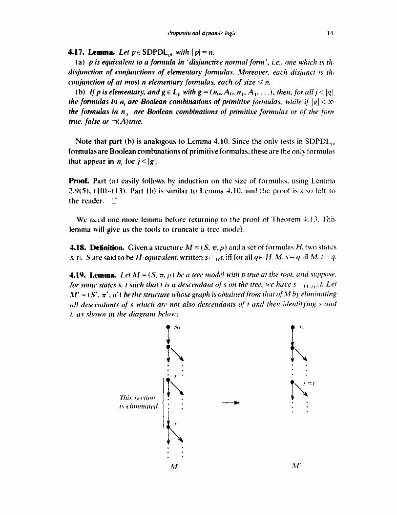
4.18. Definition. Given a structure M = (S. 7x p) and a set of formulas H, two states s. t t‘ S ztre wid to he H-eq~firnlenk written s= ,,&iff for-all qE If, .%I. sk=y iff M. tl=q.
1-l-l J. Y. Halpem, J. H. Re[f
Defhe n’ so that for u E S’,
M’. uI=q if qEFL,(p) a&M, ui=q.
Then M’ is tableau for p.
Proof. All the tableau conditions except Definition 3.3( 12) immediately follow
from the construction of R/I’. Now suppose M’, s,,t= (while r do a od)q (the case for
states other than so is identical ). Then by definition of 7~’ we also have M, s,,I= (while r do a od)q. Thus there is a path g = (/lo, At,, . . . , AL, ok) E Lwhilerdoccod which is con-
sistent with some trajectory (so,. . . , sk) E ~,$~(while r do ti od) and M, sk I= q. If this
trajectory does not pass through S, then it also exists in A/1’ and we are done.
Otherwise, suppose s = s,. Then by Lemma 4.14(a) there is a formula q, cz
FL+((while r do a od)q) c FLJ p) such that q, is of the form (,~$)(h,) l 9 l (II,,)+ where
and
want to truncate the infinite 11,‘s without affecting the finite paths. To this end, let
Then if lg,l= a and g, = ( I (tr A,,, q1 A 1. . . -1, let
By Lemma -US(d), g: E L,,. Truncate the infinite trajectories consistent with those
g, such that Ig,l = IX? to finite trajectories of length IV. Note the truncated trajectories
are now consistent with g,‘. Let S’ be the union of the states in the truncated
trajectories, and let M’ be the subtree of A4 determined by S’. Then, by Lemma 4.17(b), it follows that for all js k there is a trajectory in M’ beginning with so
which is consistent with ,q, (or gJ if g, is infinite). Thus M’, s(,+ rI A . - - A rL, so we
also get M’. S,+= p,,.
:\I’ is a finite tree model with d tz branches, but we are still not done since we
require a model whose branches have length ~2”. Here Lemma 4.19 comes into play.
First note that by systematically replacing subformulas of p(, of the form ( p A q) by (p?)q. we can find a formula p1 of SDPDL such that 1 p21 = tI and l=p,, = y,. NOM suppose ( s, ,. . . . , s,,,) is a branch in ,&I’ of length >2”. Then there must be two states
s,. s, on the branch with s, a descendant of s; and s,= I I_,,,h, s,, since it is easy to
check that there are at most 2”s r I ,,, ,: equivalence classes. LA A4 = (S”_ 7~“~ p”) be
the htructurc whose graph is obtained from that of M’ by identifying s, and s, as
in Lcmmtt 4. IO. Then AI” is a tablez for p2. By Lemma 3.4 we can convert AI”
to a model with a graph isomorphic to that of M”. By repeating the procedure
described above a finite number c>f times. we can find a model for p2. ,lnd hence I),,. Ah tt branches all of length -2”. I2
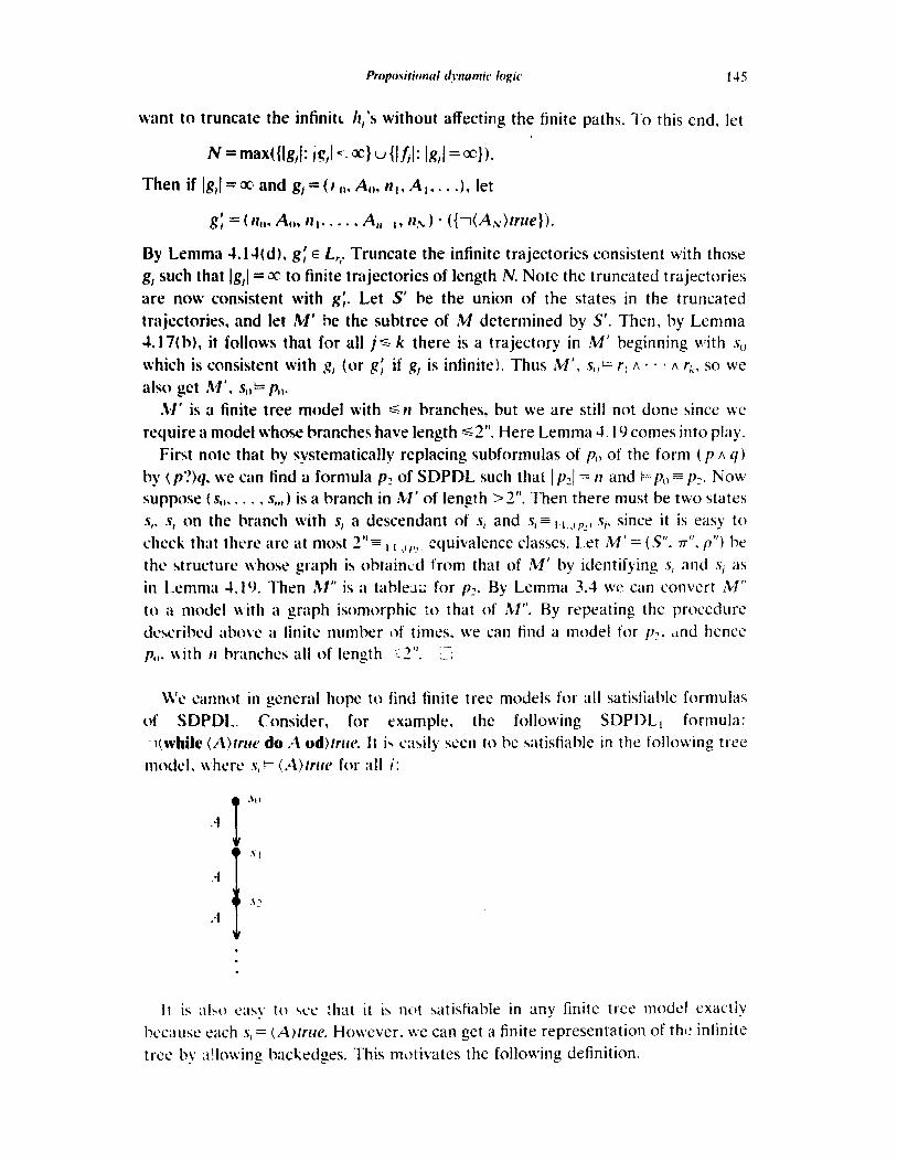
We cwnot in general hope to find finite tree models for a11 satisfiable formulas
of SDPDL. Consider, for example. the following SDPDLI formula: l(while (A)rnre do .-I od)fnre. It i\ easily seen to be satisfiable in the following tree
m0dtA. \4 hcrc s, k= (A)lrrre for 41 i:
It is alw easy to we that it is not satisfiable in any finite tree model exactly
twcauw each s: I= (A)tnre. However, we can get a finite representation of th(z infinite
tree by a!lowing backedges. This mk>,tivates the following definition.
146 J. Y. Halpern, J. H. Rejf
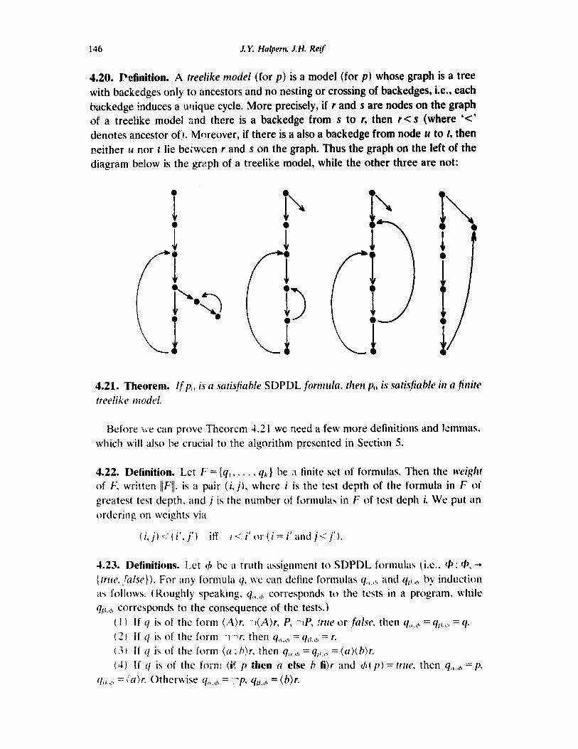
4.20. Definition. A treelike model (for p) is a model (for p) whose graph is a tree with backedges only to ancestors and no nesting or crossing of backedges, i.e., each backedge induces a uflique cycle. More precisely, if r and s are nodes on the graph of a tree’like model 2nd there is a backedge from s to r, then r< s (where ‘<’ denotes ancestor of:). Moreover, if there is a also a backedge from node II to f, then neither u nor t lie beiwcen r and s on the graph. Thus the graph on the left of the diagram below is the greph of a treelike model, while the other three are not:
4.21. Theorem. If p:, is a sati@ahle SDPDL j’~rt~rk~. than pf, is scltiyfidh irl CI fittite
treelike model.
&fore we can prove Theorem 4.; 3 I we need a few more definitions and Ji’mmas. which will also be crucial to the algorithm presented in Section 5.
4.22. Definition. Let F ={q,, . . . , dlk} be ;I finite set of formulas. Then the wight
of F;I, written ilFj_ is a pair (i, j,, where i is the test depth of the formula in F cd greatest test depth, and j is the number of f~)rmula~ in F of test deph i. 1% put WI
ordering on weights via
hopositional dynamic logic 147
(5) If q is of the form (while p do a od)r, and 4(p) = true, then qn.& = p,
qo.& = (a)(wbile p do u od)r. Otherwise q,,,4 = lp, qB,4 = r.
(6) If q is of the form (p?)r, then qa.& = p, qB,d, = r.
(7) If q is of the form ~(a ; b)r, then qm.& = qP.4 = +z)(b)r.
(8) If q is of the form l(if p then a else b fi)r and 4(p) = true, then %a4 = JJ and qp,& = -I(&. Otherwise, qcl.& = lp, qP.& = +)r.
(9) If q is of the form l(while p do a od)r and 4(p) = true, then qa,d = P, qPadi = l(u)(while p do a od)r. Otherwise qn,& = lp, qp.& = lr.
(10) If q = l( p?)r and (b(p) = trzle, then qa.& = p, qP.& = lr. Otherwise qa,c6 =
%a = 1p.
Given a set of SDPDL formu& F, let T( F, 4) be the least set of forn?ulas
containing F such that if q E T( F, q+), then qtr.,,, qP,& E T(F, 4). Given a model A4 = (S, n, p) and a state s E S, we will say (b agrees I&‘: s if
(b(q) = trzre iff M, sl=q.
4.24. Lemma. Let F c FL,( p,,), where Ip(J = n, and let 4 be any trrith assignment. T/ten :
(a) T( F. d4 c FLJ po). (b,) T( F. 6) = Us” , Ft. where F(, = F and
L (q E Fl 1 q is of the form (A)r or l(A)r}.
Moreocer, II& ,I( d llF$ (c) If 4 agrees with s urzd M, si= q for all q E F, then M, st== q for all q E T(F, 4).
Proof. Parts (a) and (c) are immediate from the definition of T( F, 4). If FE FL,( p,,),
then I T( F, &J Q 2n, so it is easy to see that we must have FL,,+ 1 = E;,!. The first half
of part. (b) follows from this observation. For the second half, we ?;im’ply note that
both q,z.,,, and 913_,t, have depth less than or equal to that of q, and if qt,.h # qp,dj9 then
~;l,,.,.,, hah depth strictly less than that of q. Cl
4.25. Definition. Given a truth assignment 4, define the relation * on formula- truth assignment pairs to be the least reflexive transitive relation such that
Given a tableau M = (S, n, p) we can similarly define*on formula-state pairs to
be the least rekxive transitive relation such that
(a; iq* sW(qP.o, s) if (q, @)+(qp,&, 4) and 4 agrees with S,
(b) ((.4)q, s)*[q, t) if M, sk(A)q and (s, t)Ep(A!.
148 J. 1: Halpern, J. H. Rejf
Note that we deliberately use the same symbol + for both relations to emphasize
their similarity. It should be clear from the context which one is meant. Intuitively,
the relation + traces the progress of a formula towards getting fulfilled. This is
made more precise by the next lemma.
4.26. Lemma. Let M = (S, v, p) be a tableau. Let p be a forrnda of the form (a)q such that M, s k p, ard /et 4 be a truth assigmerzt that agrtx’s with s.
W Either ((a)q, 4H(q, 4) or ((a)q, #)+r, &), where r is of the fmn (A;(b,l - - . (b&
(13) Let a = ( so, . . . , sk) E ql (a), k ) 0 such that s = s,, ami M, sk I= q. Let gh be a
path with ,g =I ( tq,, A+ . . . , A h l, rlli ) E LLI. h E L,, such that g is consistent with a. For i C- k. let pI be the formula of the form (A,)( b,) l l . (bk)q E FL,((a)q) which exists h I Lenrmr G.lA(a). Then M, .~,I=;:,, arzd (11, sM(pi. s,).
Proof. The proof is very similar to that of details here. !I
Lemma -!. 1 -t(;d, so we omit further
Proof of Theorem 4.21. We show by inductil on on the weight of F C_ FL,( p,,) thut
Using Lemma 4.24(b) to obtain the second inequality, we can easily check that
IlC 4 u l l l u Gil d II&11 5 $%ll = IlFll.
Since it is also easy to check that we cannot have i;G,Il= 1lG,ll= ]IFll if i # j, it follows
that if f,, has successors on the graph, their weight must be less than or equal to
that of to, and at most one of the successors can have weight equal to to. If to does
have successors on the graph, we will call the one of greatest weight tl. If /t,ll= [itl&
we repeat the above process with t, in place of to. Eventually one of two things will happen. Either the process terminates and we
have a finite sequence of nodes to, . . . , t,,, such that Iltc,ll = . - l = Ilt,,,ll, and all other
nodes on the graph have lower weight, or there is an infinite sequence of no$es
to* t ,, . . . , all of which have the same weight. and again all the other nodes on the
graph have lower weight. In both cases every node on the graph other th;in the
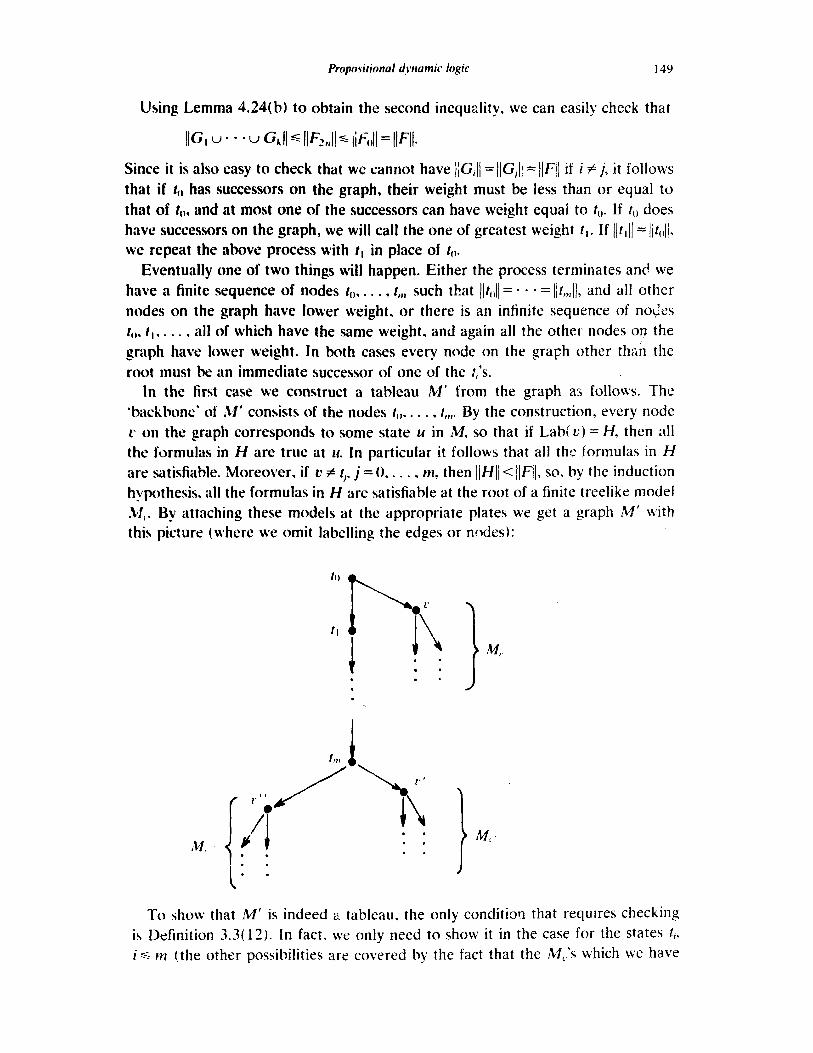
root must he an immediate successor of one of the 2,‘s. In the first case we construct a tableau M’ from the graph as follows. The
‘backbone’ of AI consists of the nodes I,,, . . . , r,,,. By the construction, every node
L‘ on the graph corresponds to some state u in M, so that if Labi u) = H, then all
the formulas in H are true at U. In particular it follows that all the formulas in H
are satisfiable. Moreover, if L‘ # t,. j = 0,. . . , MI, then jlHll< llF/l, so, by the induction
hypothesis. a11 the formulas in H are satisfiable at the root of a finite treelike model
l ,. By attaching these models at the appropriate plates we get a graph M’ with this picture (where we omit labelling the edges or nQdes):
To show that M’ is indeed z, tableau, the only condition that requu-es checking
is Definition 3.3( 12). In fact. we- only need to show it in the case for the states t,, id HI (the other possibilities are covered bv the fact that the M,.‘s which we have s
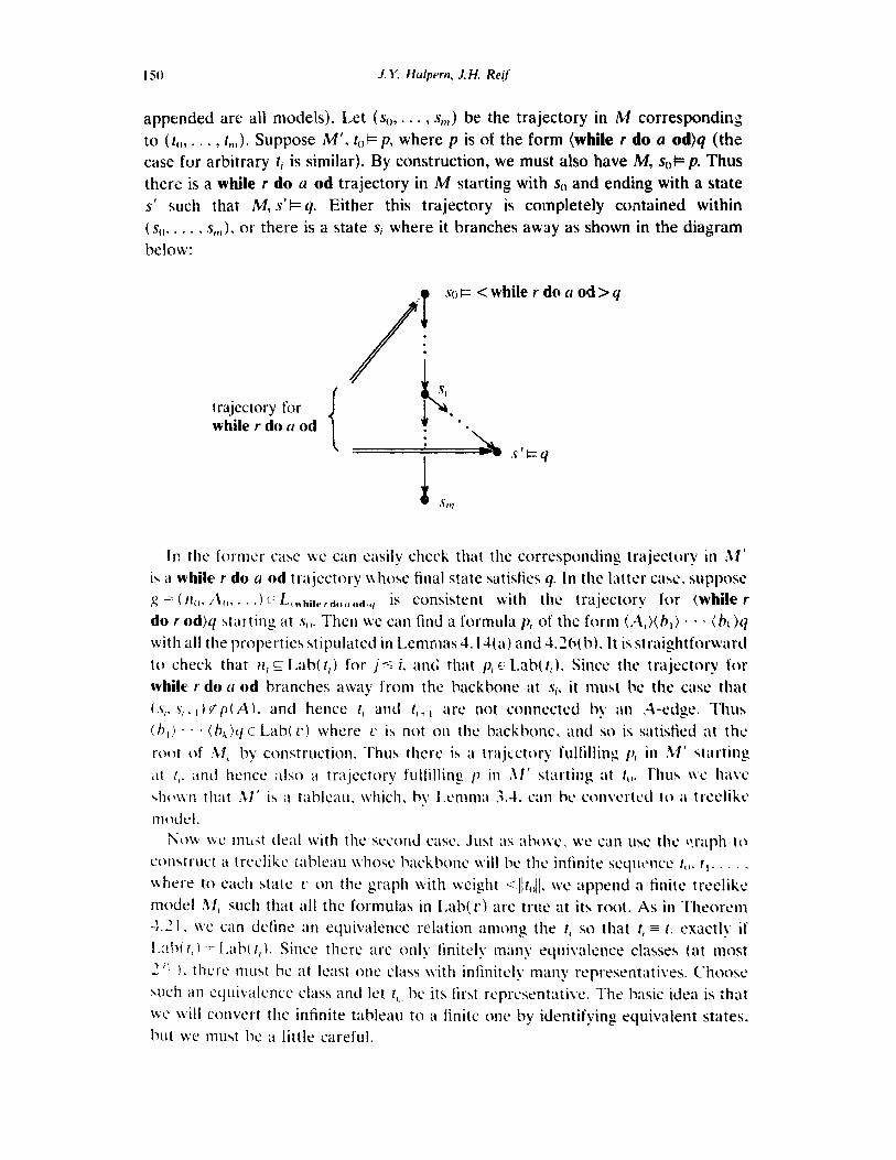
150 J. Y. Halpern, J. H. Re[f
appended are all models). Let (so, . . . , s,,,) be the trajectory in M corresponding
to (20, . . . , t,,, ). Suppose M', tc, I= p, where p is of the form {while r do a od)q (the
case for arbitrary ti is similar). By construction, we must also have M, sol= p. Thus
there is a while r do a od trajectory in M starting with so and ending with a state
s’ such that M, s'l= q. Either this trajectory is completely contained within
( so. - - - , s,,,), or there is a state Si where it branches away as shown in the diagram
below:
trajectory for while Y do cl od
< while r bdcraod>q

hposirionul dynamic logic
The problem is best exemplified by a model M . structure:
ICJ
with the following treelike
Suppose f,‘(, is the formula (while P do A;A od)trtie. and M, s-, I= -IP while, for i # 2,
M, S,kP. It is easy to check that A4 so I= p,,, and that sl =), ,( ,+,, s3. However, if we identify s, and sI as in Lemma 4.10, we no longer have ;i tableau for p(, since there
is no trajectory fulfilling while P do A ; A od starting from s,,. In Lemma 4. I9 we
considered only tree models. so we could count on there being a trajectory below
sI which. when appended to the trajectory from s,, to .q, would fulfill (while P do A : A od)q. Here. because of the backedge this is no longer the casz.
Our \tratcgy will be to rt i&n enough states to ensure that all the form::las in
Lab( !,,,I of the form (a)9 get fulfilled.
LC1 91. . . . . y,,, bc all the formulas in Lah( r,,) of the form (N,) * - ++,jq, where q
i> not of the form (b)r. We know that M, s,,,b q, A . - - A q,,,. Turning our attention
to q, for the moment, we argue just as for (while p do (1 od)q &ove that there is
;L htatt‘ s,, such that (s,,,. . . . , s,, 1 i: T(LI,; - - - ; al,) and M’, s,, k q or the 7( cr,; * * . ; u,,)
trajr‘ctor~ in ,\I starting at s,, branches awa!~ from (s,,. sj. s2, . . .I at q. Similarly for y:. . . . . Cl,,, w can find states s,,, . . . . s ,,,,. We can assume without loss of generality
that i, T- i> I - . l 5~ i ,,,. Choose N > i,,, such that r,,, = ty. We get a new treelike tab!eau
M” 11~ identifying t,, and t %, and eliminating all the states in AI’ below tJy (see the
diagram at the top of p. 153.
Hut t1 = 1,. so rc Lab( t,,). By the same argument as we used in the first case above.
we can show that there will be an a,; - - - : a,,-trajectory starting at I,, fulfilling r, SO
wt‘ are done. Z
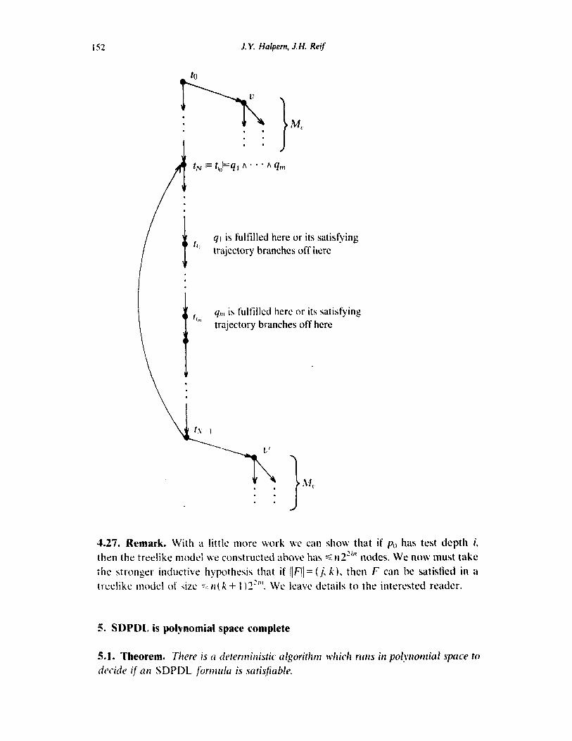
152 J. Y. Halpern, J, H. Reif
t0
2J -‘h . . M . . .
l . I . . I t q1 is fulfilled here or its satisfying 11 trajectory branches off here t In:
Y,,~ is fulfilled here or its satisfying trajectory branches off here
5 SDPDL is polynomial space complete V.
Propositional dynamic logic 153
Proof. Let p. be an SDPDL formula, p(,) = n. For reasons of clarity we will initially
present an algorithm which is not optimal with respect to space, but nevertheless runs in polynomial space. We will make some remarks on improving the algorithm at the end of the proof.
The algorithm essentially tries to construct the treelike model for p. guaranteed
to exist by Theorem 4.21, without the benefit of the tree model as an oracle. Thus
it needs to nondeterministically guess what the oracle would have said. Note that
we will need Theorem 4.21, which says that such a model exists iff p. is satisfiable,
to establish the correctness of the algorithm. Finally, we use the result of Savitch [ZB] which allows us to eliminate nondeterminism and still have a polynomial space
algorithm. At all times the algorithm will be working on a subset of formulas of FL,( p,,)
analogous to the F of Theorem 4.21. There will also be polynomially many other
such subsets on a pushdown stack, waiting their turn to be worked on. As in Theorem
4.2 1. these subsets correspond to (the labels of) states of the tableau. Since we can work on only one branch of the tableau at a given time, the sets on the stack represent formulas for which the tableau conditions will be satisfied along a branch
of the tableau other than the one on v+hich we are currently working. With each
subset is (possibly) associated one other subset which we call the backpointer. If
there is an associated backpointer, then some formulas in the backpointer will be
associated with formulas in the first subset. Intuitively, the backpointer corresponds
to the state t,, in the second half of the proof of Theorem 4.21, i.e., the state to
which a backedge (if there is one) will go. (Remember that we are constructing a tree/&e tableau.) Thus the backpointer must have the same weight (in the sense of
Definition 4.22) as the first subset. If the first subset corresponds to state s on the
tableau while the backpointer corresponds to state t, then formula q in the backpoin-
ter will be associated with formula q’ in the first subset precisely if (q, t)=+ (q’, s).
Thus we will be able to keep track of the progress of formulas in the backpointer
towards getting fulfilled. We will be able to branch back in our construction exactly
when the backpointer is identical to the first set and there are no further formulas
wa’iting to be fulfilled.
lnrtially we work on (p(,}; the stack is empty. Suppost: at a certain time the
algorithm is working on the set F = {qr, . . . , qk} c_ FL,( p,,). We nondeterministically
guess a truth assignment 4 and compute T( F, 4) as in Lemma 4.24(a). (-Vote we only need to guess the value of 4 on the formulas of FL,( p,,).) Then:
Stq~ 1. If (r, -jr} c T( F, 4) for some formula r, we terminate with “unsatisfiable”
(the particular sequences of choices made by the algorithm was bad). Step 2. For * given as in Definition 4.25, we check that Lemma 4.26(b) holds.
‘That is, for q~ T(F, c$) of the form (a)r, we check that either (q, @*Vq b) or
there csists r’ of the form (A)(b,) l . - (b,,,)r such that ((7, d))=+(T), 4). If not, we
terminate with “unsatisfiable”. Suppose that the primitive programs mentioned in p. are A 1, . . . , A. W then
form the sets G,, . . . , Gk just as in Theorem 4.21. If there is no backpointer
151 .I. Y. Halpern, J. H. Reif
associated with the original set F, we can nondeterministically choose to associate F with a copy of itself as a backpointer, in which case we associate every forlnula
in the copy of the form (a,) : l . (a& with the same formula in E Step 3. If F has no associated bazkpointer, we immediately go to Step 4. Other-
wise, we must check that one of the G,‘s has wc;ight equal to 11F;‘11. (By the equalities of Theorem 4.21, we know there can be at most one.) If not, we terminate with “unsatisfiable”. Otherwise we associate the backpointer H with G,, where 1lG,ll =llFll
l =liH[l). If ah t e ‘ormula pl E H is associated with P~!E F, and (pz,4)*((A& di) (for the C$ chosen above), we associate p1 with TE Gi. If Gj = N and none of the formulas in H are associated with a formula in G,, we set G, to the empty set and forget
about H. (Essentially we have branched back, so we do not have to worry about
satisfying this set of formulas any more. We can continue working on the other sets in the stack.)
SZep 4. If all of G,, . . . , G,, are empty, then we work on the top clement in the
stack. If the stack is empty, we have succeeded in finding a treelike tableau tar p:
we terminate and return “satisfiable”. Step 5. If some of the G,‘s are nonempty, we work nest on the one of lo,west
weight, putting all the rest on the stack. If there is more than one G, of lowest
weight, we choose one of these arbitrarily to work on nest.
(Note that in Theorem 4.2 1 we used as a11 inductive hypothesis that s,ltistiablc sets of lower weight had an appropriate treclike model. Here wt: actually verify that the sets of lower weight have ~nodcls hcforc dealing with the sets of higher
weight. which get put on the stack.)
If a sequence of choices mad< by the algorithm returns “wtisfiablt”‘. the proof
of l’h~orem 4.21 shows that we have indeed constructed a trwlikc tablc‘au for I),,.
so p,, reallv is satisfiable. Conwxsely, if I~,,c SDPDL, is s;Miable. w know hj _ Theorem 4.21 that therr: is ;i finite trtxlikc tabltxu fit- I>,,. If the algorithm nides
guesses correspondiy i:O tk state of aflairs 01i this tableau, it will output “satisfiable”.

Propositional dynamic logic 155
We now sketch a method to improve the space complexity. We first note that
instead of putting GI, . . . , Gk on the stack (as in Step 3), we can instead put on
those formulas in T(F, 4) c FL,( po) of the form (A& or l(Ai)q; these in turn can
be represented by a bit string of length IFL,( po)l s 2n. We can then modify the
algorithm so that it deals with these bitstrings, and by arguments similar to those
used in the previous paragraph, we can show that when we are working on a set with the rttth highest attainable weight, there are at most nz such bitstrings on the
stack. This modified algorithm (which must also represent FL,( pC,) in a space efficient
manner, something which we claim without proof can be &one) can be shown to run in nondeterministic space 0( II’). By Savitch’s Theorem, it runs in deterministic
space O( II?. q
S.2* Remarks. ( I ) Essentially, the algorithm attempts to construct a treelike model for A, in a depth-first manner. Every time there is a choice of paths to follow, we
follow one of them and put the other sons of the node on the stack. Since we want
to work in polynomial space. we must be careful that the stack does not grow too
large. We ensure this by following the ‘path defined by the son of least weight. But
the use of weights was not essential in the algorithm because of the following general
fact: we can do a depth-first search of a tree with n nodes and outdegree k with a
stack of height d k leer, ( II 1. (Of course. the search will not necessari!y proceed down
the leftmost path; wi must guess the appropriate path to follow at all times.) The
proof follows by an induction on the height of the tree. By Remark 4.27, if p(, has
;I model, it has one of size < 112”“. so we can nondeterministically construct the
model in polynomial space. However, the use of weights does eliminate the nondeter-
minism at this stage and gives ‘1 slightly sharper upper bound CM the amount of
space required.
( 2) A similar theorem holds for SDPDL,,, formulas, but in this case the proof is
easier since. by Theorem 4.13, SDPDL,, formulas have finite tree models. This
means we do not have to take care of the possibility that a path might branch back
to a ancestor, and we do not need backpointers.
(3 A larwc schv~w is an uninterpreted deterministic program scheme with only
one program \variablc (cf. [9!). ‘Ike schemes are strorlgly equivalent if, given an>
intcrprcMon of the symbols in the schemes. they both compute the same result
or they both fail to halt. AS noted in [73. given Ianov schemes a and h we can
ctiectivcly construct PDL programs. say a’ and h’, such that a and b are strongly
equivalent Ianov schemes iiT (a’>0 2 (b’)Q, where 0 does not appear in either- a’ or
K. But UT can easily show that, without loss of generality, a’ and b’ are SDPDL,,,
programs. Thus we have a polynomial space procedure for deciding strong
equivalence of Ianov schemes.
Although we have assumed that our programs are well-structured (i e., formed from primitive programs by means of the constructs while. . . do. . . od and

1% J. Y. Hcdpem, J. H. Reif
if. . . then. . . else), our results would clearly also hold if we viewed our programs as deterministic flowcharts whose instructions consisted of primitive programs and
tests. We could then get a deterministic propositional flowchart logic by allowing
the programs to appear in the ( ) construct (cf. [26]), and prove a polynomial space decision procedure for this logic as well, using much the same techniques as presented here. Indeed, these te&niques can also be used to prove polynomial space decision procedures for several other logics of programs including linear time temporal logic (TL) and extended linear time temporal logic. (See [S] and [30] for the syntax and
semantics of these languages, as well as further details. Polynomial space results for TL are also presenled in [29].) We formalize these observations in the following
theorem.
5.3. Theorem. There is a polyrnmial space algc~rilhnt fnr &ci(iill~ satisfiability qf
forn~rrias ii1 each of the foilowir2g Iogics:
t a 1 deterministic propositiorlal flowchart logic,
( h ; DPDL with only one yrirnitive pro,qram,
f c 8 linear time teniporr!! i’qic.
t d ) exteded lirzear time temporid logic.
Propositional dynamic logic 157
deterministic, well-structured context-free programs (which simulate recursive
calls), the satisfiability problem for the resulting logic is undecidable (and, in fact, fI i complete).
The basic requirements for a logic to have a polynomial space decision procedure
seem to be that there be an analogue to the Fischer-Ladner closure of size polynomial in the length of the formula, and that an analogue of Theorem 4.12 holds, i.e., that
every satisfiable formula be satisfiable in a tree model with only polynomially many nodes at every depth. As we will show in the next section, the anslogue to Theorem
4.12 does not hold for DPDL with two primitive programs. Results of Parikh [ 1 Y]
combined with those of Fischer and Ladner [7] also show that the decision prozzedure
for DPDL with two primitive programs is complete in exponential time.
(2) We note that a formula p of TL can be translated to, a formula $ of DPDL with only one primitive program such that p is TL-satisfiable iff pf is DPDL-satisfiable
by using the following unductively defined procedure:
Pt = P for an atomic formula P,
(Gp)’ = [A*]& ( puq)’ = t(( p’)?; A)*)q’. We leave to the reader the task of checking that the translation has the required
property. In Section 6 we will show that each transl*:ted formula is actually equivalent to an SDPDL formula of essentially the same length. Note that this also gives us
anot her proof of Thccrem 5.3(c). Similar results can also be shown for ETL. We
omit details here.
5.5. Theorem. The decision problem for :<DPDL,,, artd hettce SDPDL, is polynomial
spa c-e ha rd.
Proof. We use ideas that arc similar to those used in Cook’s proof that SAT is
NP-hard; (cf. [ 14, pp. 325~3271). Given L E PSPACE, we can assume without loss
of generality (cf. [ 13, p. 2891) that f, is accepted by a one-tape deterministic Turing
!Machine . !;I which, for some polynomial p, runs in space sp( tt) on inputs of length
tl. WC will construct an SDPDL,, formula f(x) which simulates the computation of .ff on input x. where j’(x) is computable in polynomial time (and log space) from
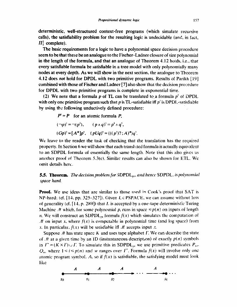
s. In particular, f(x) will be satisfiable iff JH accepts input .Y. Suppose .Irl has state space K and uses tape alphabet K We can describe the state
of . If at a given time by an ID (instantaneous description) of exactly p(n) symbols
in I“ = (K x I‘) u 1‘. T o simulate this in SDPDL,, we use primitive predicates P,,.,,
QW where 1 G is p(n) and fi’ ranges over IT’. Formula f(xj will involve only one
atomic program symbol. A, so if f(x) is satisfiable, the satisfying model must look
like
A A A A . . . --q . . .
so St 82 Sk

158 J. Y. Halpern, J. H. Reif
The intuition is that Phsi wiii be true at state Si iff, when we run ..& the ith position on the tape at time i contains symbol w. (If w = (9, Z) E K X f, then the head of -44 is also at the ith position reilding symbol z and the machine is in state 4.) Moreover, P,,., is true at state si iff c,rpi is true at state s,+ I. Thus the Qwi keep track of the values of the P,,i at the previous time.
The formula f(x) will have to state the following: ( 1) The only P\+ti’s true at so are those that describe the initial ID. (2) In every state s, up to the time x is accepted, the P\\,i’s that are true in S,
correspond to a string of symbols, in that for all i there is a unique w E r’ such that Pb1.i is true.
(3) P,*i is true at S, iff Q1s.i is true at Sltl.
(4) The ID true at state S, follows from the one true at si. I (for ia 1) by the
indicated move of 3. We take f(s) to be the conjunction of the four formulas f,(x), f&x). f3(x) and
fi(s f. which enforce conditions ( 1) through (4) respectively. Let .Y = xr, l l l x,, ,.
where x, E I’. let 9(, be the initi,rl state of . tt, and let h E I’ denote the blank symbol. Let sfring he the formula which says that the P,,.,‘s correspond to a string of
\ym bols:
Propositional dynamic logic
the formula consistent:
159
A ( V QM.I I A Qm A @.I+ I h pzi * I- I’ p(H) (1fl.t,~.~~IR~rl.I:.~.~)} )
Then fJ(x) is the formula
(while -?accept do (A ; consistent?> od)true.
Cleky if x E L, then f(x) is satisfied in a model such as the one above, where there are k states corresponding to the k steps of the accepting computation by A.
Conversely, if M, q+=fcx), then the graph corresponding to .ti looks like the one
pictured above, except that it may be an infinite straight line. Let k be the least
number such that M. sA k accept. Then it is easy to check that .M accepts s in k
steps, where l , s,b PHI iff w is in the ith position of the tape at time j. Cl
From Theorems 5.1 and 5.5 and the fact that p. is valid iff --up is not satisfiable we immediately obtain the following.
5.6. Corollary. The sati$ability and mlidity problems for SDPDL arid SDPDL[,,
tire polyomial space complete.
5.7. Remarks. ( I 1 In [ I] it was already shown that every satisfiable DPDL (and
hence SDPDL) formula has a model‘of size ~4%‘. The question arises if we can do any better for SDPDL formulas. The answer is essentially “no”, since by using
the techniques of Theorem 5.5 we can encode the computation of a Turing machine which counts up to 2” anu then halts into an SDPDL formula. This formula will
have size O{n). and the smallest model that satisfies it will have size 2”.
(2) Similar proofs can be used to show that all the logics of Theorem 5.3 have
decision problems complete in polynomial space.
6. Expressiveness
6.1. Definition. For two logical languages .I/’ and . N. we say . M is at least as expressive
;IS K and write Y’s, 11, if-f, for every formula pi ;It, there is a formula p’ E .6! such
that or p = p’. ./I and ‘/ s r cl e said to be equally expressive, written Y’=. ld, if -Y-g .li
and . It s Y. Y is less expressive than .I!, written Y’< .M, if Y< N and YXZ4.
Peterson [2 I], Berman 123 and Berman and Paterson [3] show that, for all i :=O.
PI-X, c: PDL, l ,. In fact. these proofs also show (S)DPDL, < !S)DPDLi+,. We USC
our structure theorem (Theorem 4.12) to rederive these results and extend them
to show that SDPDL, < DPDL, and SDPDL < DPDL.
6.2. Remark. Meyer and Winklmann [ 171 show that SDPDL,, < DYULF,I by show-
ing that the DPDI.,,, formula iA*)[A”]P is not equivalent to any SDPDL,,, formula.
160 J. Y. Ha/pet-n, J 5. Reif
Their proof does not extend to t)l!i SDPDL. It is easy to see that, for any formula
P*
I== (A “)p 5: (while --y do A od} true
and hence
I= [A*]p := [while p do A od]jaIse.
From this rema.rk it is easy to see that (A*)[A*]P is equivalent to an SDPDL formula. (Moreo\fer, this observation, combined with Remark 5.4(2), also shows how to translate TL into SDPDL.j However we still get the following theorem.
6.3. Theorem. For 011 i 2 0, we hoe SDPDL, < SDPDL,, , ami SPPDL =c DPDL.
Proof. Let z‘,, = {A, B), and let M be a model whose graph is a full binary tree L w rooted as s,, as illustrated below:
161
Combining these results with those of Peterson [21] and Berman [2], we get the
following picture. where languages not connected by a chain of c’s are incomparable
in expressive power:
DPDL,, c DPDL, <. . l < DPDL
V b J -
SDPDL,, < WPDL, < l l 9 < SDPDL.
7. A complete axiomatization for SDPDL
In [ 11 it was shown that by adding the axiom schema (A)p + [Aju to the Segerberg
;~xiom~ for PDL we obtain a complete axiomatization for DPDL. Since SDPDL is
a restriction of DPDL. this automatically gives us a complete axiomatization
of SDPDL. However. we would still have to have an axiom;ltization that respects
the syntax of SDPDL. We present such a system below. Essentially all we do is re- piace axiom< about u and * by their appropriate analogues involving
if. . . then. . . else. . . fi and while.. . do. . . od. The axioms presented are based on
thaw suggested by Passy (cf. [Xl) who proved that thiv system without axiom (8)
~;ts complete for ;I \wiant of SDPDL in which the primitive programs were not
;wumed to be deterministic (note the analogy between PDL and DPDL here.) A
Gnilar ;komatizution was suggested by Chlebus [6].
7.1. Axiom Schemes snd inference Rulec. Consider the following deductive system
for SDPDL (dw-e w ;wunw that A is now a symbol in the language):
(0) ---- ( p fi y) -[tr]q
q + [while p do n od]y .
7.2. Theorem. Axiom schemes and rules ( I ) -( 1 1) above give a complete axiornatir-
afiorl for SDPDL.
Proof. We essentially follow the lines of [ IS] atld [I]. We say that a formula p is prouabfe, and write t- p, if there exists a finite sequence of formulas, the last one
being p, such that each formula is an instance of an axiom scheme or follows from
previous formulas by one of the inference rules. A formuhr 11 is cortsisfcrlf if not
k- up, i.e., if ---up is Got provable in this system. We want to show that any valid
SDPEL formula is provable. It suffices to show that if /I,, is consistent, then p,, is
SDPDL satrsfiable.
Call a subset of FL,( [I,,) maximal iff for every formula --1(1 E FL,( II,,), either y c s
or -MI c s. If 0 is a subset of FL( II,,), let p,, the atom msociateti with s, bo the formula
A’,. 4
s E n( p) iff P)E s (or equivalently, iff PC FL,( A,) ;mi t-p, + 11).
(s. f ) f p( A ) iff p, A (iI)p~ is consistwt
Since p, is consistent. so is p, A (A)p, for some t E S with 9 E t. For this c we have
(s. tk p(A) and M. U==Q. For tableau condition ( 111, suppose by way of contradiction that M, s I= --l(A)y,
hut for some I with (s, I) c p(A) we have M, z I= 9. Thus it follows that
I- P\ --p, -Wq. c-p/ 3 q and pS A ( A)p, is consistent.
Using Axiom Schemes (6). ( 10) and ( 1 I ) and propositional reasoning, it follows that -$A)g A (A)9 is consistent, and this is a contradiction.
To check (3). suppose that M, s k (A)(!, but for some I with (s, t) c p(A) we have
.V. I C= -7q. As above we get
t-p, -44q. +p, + Tq and p, A (A@, is consistent.
7.2.1. Lemma. If thercD is a formrkl (?f tk form (o)q E FL, ( p,,) ard p, A ( CJ)~, is ciw:i.wwt jar s. t I s. tkr1 ( s. t ) f p ( L1 ).
3 ( p, /> - 19 ) v lb b(while 9 do h od)( p, A -xi )
= fdse v (h)(whilc 9 do h od)f~~I.se (since k-p, -+ y 1
J. Y. Hdpem, J. H. Reif 164
Acknowledgment
We would Iike to acknowledge the anonymous referees for their comments and suggestions on clarifying the presentation of these results.
References
Propositional dynamic logic 165
V.R. Pratt. Semantical considerations of Floyd-Hoare logic. in: I7rh IEEESywtp. on the Foundations
of Computer Scietrce ( 1976) pp. I OY- 12 1. V.R. Pratt, A practical decision method for propositional dynamic logic. in: I WI Ann. ATM Symp ON the I’kory of Computation ( 1978) pp. 326-337; revised version: A near optimal method for reasoning about action, J. Comput. Systems Sci. 20 (2) ( 1980) 231-254. V.R. Pratt, Models of program lo&s, in: 20th 1EEE Svmp. on the Fouruiatiom of Conqxmr Science . (lc179) pp. 115-122. V.R. Pratt, Using graphs to understand PDL, in: D. Kozen. ed., Proc. IBM Corlf on Logics of
Pmgmrrrs, Lecture Notes in Computer Science 131 (Springer, Berlin, 1982 t pp. 357-396. A. Snlwicki, Frwmalized algorilhnric I;mguitgcs, Bull. Acad. fol. Sci., Ser. Mcrfh. Astr. Ph_vs. 18 (5) (1970) 227-232. W.J. Switch. Relationships between nondeterministic and deterministrc tape complexities.
J. Contpttt. Systems Sci. 4 ( 2 ) ( 1970) pp. I 47- 1% tl. I’. Si\ll;t and F.M. C%rkc, The complexity of propositi.wal linear temporal lo@. in: 1-M Atw. .4<W Synrp. i,t the Thcor~ of Comprrtatiorl ( 19X2) pp. 159-i 60.
Top Related