


Languages
Pages
Legal

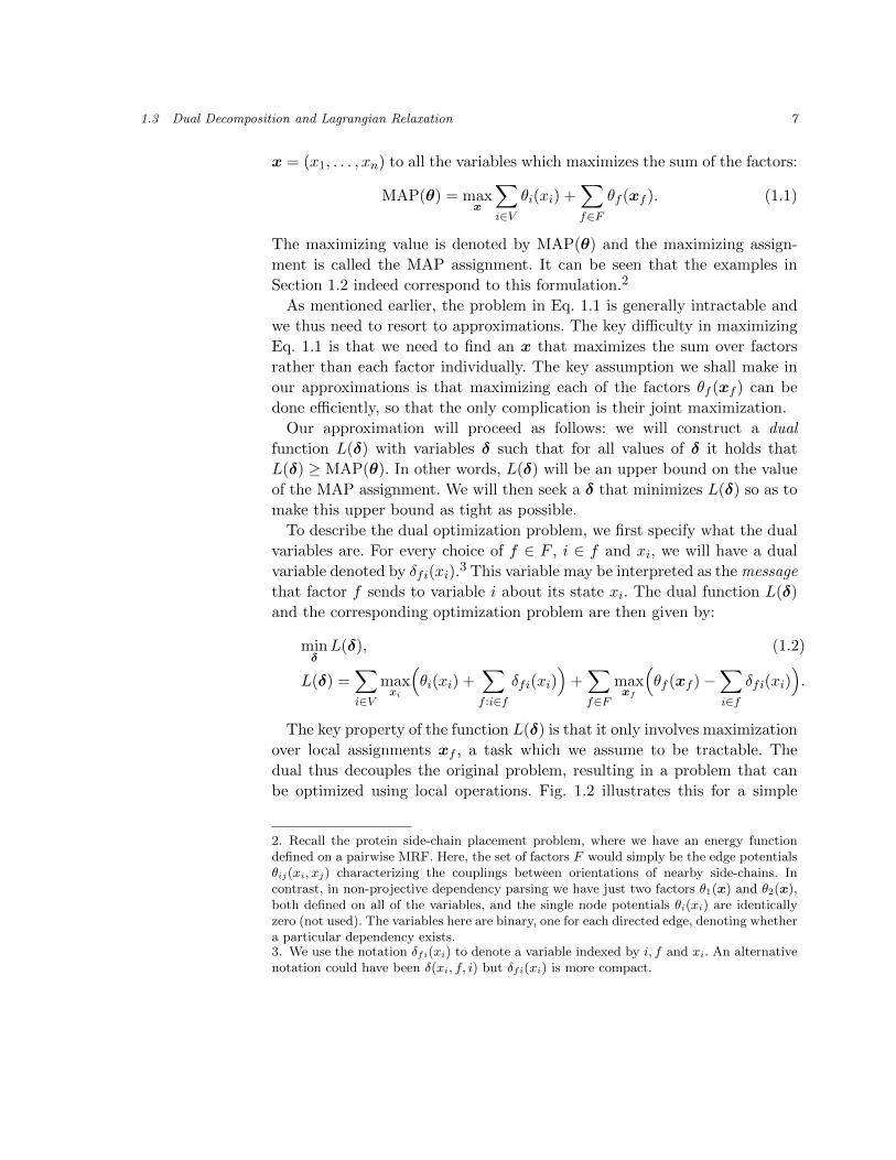
1 Introduction to Dual Decomposition for
Inference
David Sontag [email protected]
Microsoft Research New England
Cambridge, MA
Amir Globerson [email protected]
Hebrew University
Jerusalem, Israel
Tommi Jaakkola [email protected]
CSAIL, MIT
Cambridge, MA
Many inference problems with discrete variables result in a difficult com-
binatorial optimization problem. In recent years, the technique of dual de-
composition, also called Lagrangian relaxation, has proven to be a powerful
means of solving these inference problems by decomposing them into simpler
components that are repeatedly solved independently and combined into a
global solution. In this chapter, we introduce the general technique of dual
decomposition through its application to the problem of finding the most likely
(MAP) assignment in Markov random fields. We discuss both subgradient
and block coordinate descent approaches to solving the dual problem. The
resulting message-passing algorithms are similar to max-product, but can be
shown to solve a linear programming relaxation of the MAP problem. We
show how many of the MAP algorithms are related to each other, and also
quantify when the MAP solution can and cannot be decoded directly from the
dual solution.

2 Introduction to Dual Decomposition for Inference
1.1 Introduction
Many problems in engineering and the sciences require solutions to challeng-
ing combinatorial optimization problems. These include traditional prob-
lems such as scheduling, planning, fault diagnosis, or searching for molec-
ular conformations. In addition, a wealth of combinatorial problems arise
directly from probabilistic modeling (graphical models). Graphical models
(see Koller and Friedman, 2009, for a textbook introduction) have been
widely adopted in areas such as computational biology, machine vision, and
natural language processing, and are increasingly being used as a framework
for expressing combinatorial problems.
Consider, for example, a protein side-chain placement problem where
the goal is to find the minimum energy conformation of amino acid side-
chains along a fixed carbon backbone. The orientations of the side-chains
are represented by discretized angles called rotamers. The combinatorial
difficulty arises here from the fact that rotamer choices for nearby amino
acids are energetically coupled. For globular proteins, for example, such
couplings may be present for most pairs of side-chain orientations. This
problem is couched in probabilistic modeling terms by associating molecular
conformations with the setting of discrete random variables corresponding
to the rotamer angles. The interactions between such random variables
come from the energetic couplings between nearby amino acids. Finding
the minimum energy conformation is then equivalently solved by finding the
most probable assignment of states to the variables.
We will consider here combinatorial problems that are expressed in terms
of structured probability models (graphical models). A graphical model is
defined over a set of discrete variables x = {xj}j∈V . Local interactions
between the variables are modeled by functions θf (xf ) which depend only
on a subset of variables xf = {xj}j∈f . For example, if xf = (xi, xj),
θf (xf ) = θij(xi, xj) may represent the coupling between rotamer angles xiand xj corresponding to nearby amino acids. The functions θf (xf ) are often
represented as small tables of numbers with an adjustable value for each
local assignment xf . The joint probability distribution over all the variables
x is then defined by combining all the local interactions,
logP (x) =∑i∈V
θi(xi) +∑f∈F
θf (xf ) + const,
where we have included also (singleton) functions biasing the states of
individual variables. The local interactions provide a compact parametric
description of the joint distribution since we only need to specify the local

1.1 Introduction 3
functions (as small tables) rather than the full probability table involving
one value for each complete assignment x.
Despite their compact description, graphical models are capable of de-
scribing complex dependencies among the variables. These dependences arise
from the combined effect of all the local interactions. The problem of prob-
abilistic inference is to reason about the underlying state of the variables in
the model. Given the complex dependencies, it is not surprising that proba-
bilistic inference is often computationally intractable. For example, finding
the maximum probability assignment of a graphical model (also known as
the MAP assignment) is NP-hard. Finding the MAP assignment remains
hard even if the local functions depend only on two variables, as in the
protein side-chain example. This has prompted extensive research into ap-
proximation algorithms, some of which often work well in practice.
One of the most successful approximation schemes has been to use relax-
ations of the original MAP problem. Relaxation methods take the original
combinatorial problem and pose it as a constrained optimization problem.
They then relax some of the constraints in an attempt to factor the problem
into more independent subproblems, resulting in a tractable approximation
of the original one. Two closely related relaxation schemes are dual decom-
position (Johnson, 2008; Komodakis et al., 2010) and linear programming
(LP) relaxations (Schlesinger, 1976; Wainwright et al., 2005). Although the
approaches use a different derivation of the approximation, they result in
equivalent optimization problems.
Practical uses of MAP relaxations involve models with thousands of
variables and constraints. While the relaxed optimization problems can
generally be solved in polynomial time using a variety of methods and
off-the-shelf solvers, most of these do not scale well to the problem sizes
encountered in practice (e.g., see Yanover et al., 2006, for an evaluation
of commercial LP solvers on inference problems). However, often the LP
relaxations arising from graphical models have significant structure that
can be exploited to design algorithms that scale well with the problem size.
This chapter introduces the dual decomposition approach, also known
as Lagrangian relaxation, and focuses on efficient scalable algorithms for
solving the relaxed problem. With dual decomposition, the original problem
is broken up into smaller subproblems with the help of Lagrange multipliers.
The smaller subproblems can be then be solved exactly using combinatorial
algorithms. The decomposition is subsequently optimized with respect to the
Lagrange multipliers so as to encourage the subproblems to agree about the
variables they share. For example, we could decompose the MAP problem
into subproblems corresponding to each local function θf (xf ) separately.
The Lagrange multipliers introduced in the decomposition would then play

4 Introduction to Dual Decomposition for Inference
the role of modifying the functions θf (xf ) so that the local maximizing
assignments agree across the subproblems. The decomposition may also
involve larger components that nevertheless can be solved efficiently, such as
a set of spanning trees that together cover all edges of a pairwise graphical
model.
The chapter is organized as follows. We begin in Section 1.2 with two
example applications that illustrate the type of problems that we can
solve using our techniques. We next define the MAP problem formally and
introduce the dual decomposition approach in Section 1.3. The next two
sections, Section 1.4 and Section 1.5, describe algorithmic approaches to
solving the dual decomposition optimization problem. In Section 1.6 we
discuss the relation between dual decomposition and LP relaxations of the
MAP problem, showing that they are essentially equivalent. Finally, in
Section 1.7 we discuss how the MAP solution can be approximated from
the dual decomposition solutions, and what formal guarantees we can make
about it.
1.2 Motivating Applications
We will make use of two example applications so as to illustrate the role of
local interactions, types of decompositions, and how they can be optimized.
The first example, outlined earlier, is the protein side-chain placement
problem (Yanover et al., 2008). The goal is to find the minimum energy
conformation of amino acid side-chains in a fixed protein backbone structure.
Each side-chain orientation is represented by a discrete variable xi specifying
the corresponding rotamer angles. Depending on the discretization and the
side-chain (the number of dihedral angles), the variables may take on tens
or hundreds of possible values (states). Energy functions for this problem
typically separate into individual and pairwise terms where the pairwise
terms take into consideration attractive and repulsive forces between side-
chains that are near each other in the 3D structure.
The problem is equivalently represented as an inference problem in a
pairwise Markov Random Field (MRF) model. Graphically, the MRF is
an undirected graph with nodes i ∈ V corresponding to variables (side-
chain orientations xi) and edges ij ∈ E indicating interactions. Each
pairwise energy term implies an edge ij ∈ E in the model and defines
a potential function θij(xi, xj) over local assignments (xi, xj). Single-node
potential functions θi(xi) can be included separately or absorbed by the
edge potentials. The MAP inference problem is then to find the assignment

1.2 Motivating Applications 5
Non-Projective Dependency Parsing
!
Figure 1.1: Example of dependency parsing for a sentence in English. Everyword has one parent, i.e. a valid dependency parse is a directed tree. The redarc demonstrates a non-projective dependency.
x = {xi}i∈V that maximizes∑i∈V
θi(xi) +∑ij∈E
θij(xi, xj).
Without additional restrictions on the choice of potential functions, or which
edges to include, the problem is known to be NP-hard. Using the dual
decomposition approach, we will break the problem into much simpler sub-
problems involving maximizations of each single node potential θi(xi) and
each edge potential θij(xi, xj) independently from the other terms. Although
these local maximizing assignments are easy to obtain, they are unlikely
to agree with each other without our modifying the potential functions.
These modifications are provided by the Lagrange multipliers associated
with agreement constraints.
Our second example is dependency parsing, a key problem in natural
language processing (McDonald et al., 2005). Given a sentence, we wish
to predict the dependency tree that relates the words in the sentence. A
dependency tree is a directed tree over the words in the sentence where
an arc is drawn from the head word of each phrase to words that modify
it. For example, in the sentence shown in Fig. 1.1, the head word of the
phrase “John saw a movie” is the verb “saw” and its modifiers are the
subject “John” and the object “movie”. Moreover, the second phrase “that
he liked” modifies the word “movie”. In many languages the dependency
tree is non-projective in the sense that each word and its descendants in the
tree do not necessarily form a contiguous subsequence.
Formally, given a sentence with m words, we have m(m − 1) binary arc
selection variables xij ∈ {0, 1}. Since the selections must form a directed
tree, the binary variables are governed by an overall function θT (x) with
the idea that θT (x) = −∞ is used to rule out any non-trees. The selections
are further biased by weights on individual arcs, through θij(xij), which
depend on the given sentence. In a simple arc factored model, the predicted

6 Introduction to Dual Decomposition for Inference
dependency structure is obtained by maximizing (McDonald et al., 2005)
θT (x) +∑ij
θij(xij)
and can be found with directed maximum-weight spanning tree algorithms.
More realistic dependency parsing models include additional higher order
interactions between the arc selections. For example, we may couple the
modifier selections x|i = {xij}j 6=i (all outgoing edges) for a given word
i, expressed by a function θi|(x|i). Finding the maximizing non-projective
parse tree in a model that includes such higher order couplings, without
additional restrictions, is known to be NP-hard (McDonald and Satta, 2007).
We consider here models where θi|(x|i) can be individually maximized by
dynamic programming algorithms (e.g., head-automata models) but become
challenging as part of the overall dependency tree model:(θT (x)
)+
(∑ij
θij(xij) +∑i
θi|(x|i)
)= θ1(x) + θ2(x)
The first component θ1(x) ensures that we obtain a tree, while the second
component θ2(x) incorporates higher order biases on the modifier selections.
A natural dual decomposition in this case will be to break the problem into
these two manageable components, which are then forced to agree on the
arc selection variables (Koo et al., 2010).
1.3 Dual Decomposition and Lagrangian Relaxation
The previous section described several problems where we wish to maximize
a sum over factors, each defined on some subset of the variables. Here
we describe this problem in its general form, and introduce a relaxation
approach for approximately maximizing it.
Consider a set of n discrete variables x1, . . . , xn, and a set F of subsets on
these variables (i.e., f ∈ F is a subset of V = {1, . . . , n}), where each subset
corresponds to the domain of one of the factors. Also, assume we are given
functions θf (xf ) on these factors, as well as functions θi(xi) on each of the
individual variables.1 The goal of the MAP problem is to find an assignment
1. The singleton factors are not needed for generality, but we keep them for notationalconvenience and since one often has such factors.
1.3 Dual Decomposition and Lagrangian Relaxation 7
x = (x1, . . . , xn) to all the variables which maximizes the sum of the factors:
MAP(θ) = maxx
∑i∈V
θi(xi) +∑f∈F
θf (xf ). (1.1)
The maximizing value is denoted by MAP(θ) and the maximizing assign-
ment is called the MAP assignment. It can be seen that the examples in
Section 1.2 indeed correspond to this formulation.2
As mentioned earlier, the problem in Eq. 1.1 is generally intractable and
we thus need to resort to approximations. The key difficulty in maximizing
Eq. 1.1 is that we need to find an x that maximizes the sum over factors
rather than each factor individually. The key assumption we shall make in
our approximations is that maximizing each of the factors θf (xf ) can be
done efficiently, so that the only complication is their joint maximization.
Our approximation will proceed as follows: we will construct a dual
function L(δ) with variables δ such that for all values of δ it holds that
L(δ) ≥ MAP(θ). In other words, L(δ) will be an upper bound on the value
of the MAP assignment. We will then seek a δ that minimizes L(δ) so as to
make this upper bound as tight as possible.
To describe the dual optimization problem, we first specify what the dual
variables are. For every choice of f ∈ F , i ∈ f and xi, we will have a dual
variable denoted by δfi(xi).3 This variable may be interpreted as the message
that factor f sends to variable i about its state xi. The dual function L(δ)
and the corresponding optimization problem are then given by:
minδL(δ), (1.2)
L(δ) =∑i∈V
maxxi
(θi(xi) +
∑f :i∈f
δfi(xi))
+∑f∈F
maxxf
(θf (xf )−
∑i∈f
δfi(xi)).
The key property of the function L(δ) is that it only involves maximization
over local assignments xf , a task which we assume to be tractable. The
dual thus decouples the original problem, resulting in a problem that can
be optimized using local operations. Fig. 1.2 illustrates this for a simple
2. Recall the protein side-chain placement problem, where we have an energy functiondefined on a pairwise MRF. Here, the set of factors F would simply be the edge potentialsθij(xi, xj) characterizing the couplings between orientations of nearby side-chains. Incontrast, in non-projective dependency parsing we have just two factors θ1(x) and θ2(x),both defined on all of the variables, and the single node potentials θi(xi) are identicallyzero (not used). The variables here are binary, one for each directed edge, denoting whethera particular dependency exists.3. We use the notation δfi(xi) to denote a variable indexed by i, f and xi. An alternativenotation could have been δ(xi, f, i) but δfi(xi) is more compact.

8 Introduction to Dual Decomposition for Inference
x1 x2
x3 x4
θf(x1, x2)
θh(x2, x4)
θk(x3, x4)
θg(x1, x3)
x1
δf2(x2)
δf1(x1)
δk4(x4)δk3(x3)
δg1(x1)+
− −
− −δf1(x1)
δg3(x3)δg1(x1)
−− δh2(x2)
δh4(x4)
−−
+ x3
δg3(x3)
δk3(x3)x4 +
δk4(x4)
δh4(x4)
+x2
δf2(x2)
δh2(x2)
θf(x1, x2)
θh(x2, x4)
θk(x3, x4)
θg(x1, x3)
x3 x4
x4
x2
x2x1
x1
x3
Figure 1.2: Illustration of the the dual decomposition objective. Left: Theoriginal pairwise model consisting of four factors. Right: The maximizationproblems corresponding to the objective L(δ). Each blue ellipse contains thefactor to be maximized over. In all figures the singleton terms θi(xi) are setto zero for simplicity.
pairwise model.
We will introduce algorithms that minimize the approximate objective
L(δ) using local updates. Each iteration of the algorithms repeatedly finds
a maximizing assignment for the subproblems individually, using these to
update the dual variables that glue the subproblems together. We describe
two classes of algorithms, one based on a subgradient method (see Section
1.4) and another based on block coordinate descent (see Section 1.5). These
dual algorithms are simple and widely applicable to combinatorial problems
in machine learning such as finding MAP assignments of graphical models.
1.3.1 Derivation of Dual
In what follows we show how the dual optimization in Eq. 1.2 is derived
from the original MAP problem in Eq. 1.1. We first slightly reformulate
the problem by duplicating the xi variables, once for each factor, and then
enforce that these are equal. Let xfi denote the copy of xi used by factor f .
Also, denote by xff = {xfi }i∈f the set of variables used by factor f , and by
xF = {xff}f∈F the set of all variable copies. This is illustrated graphically
in Fig. 1.3. Then, our reformulated – but equivalent – optimization problem

1.3 Dual Decomposition and Lagrangian Relaxation 9
x1 x2
x3 x4
xf1 xf
2
xg1
xg3
xh2
xh4
xk3 xk
4θk(x
k3, x
k4)
θh(xh2 , xh
4)
θf(xf1 , xf
2)
=
==
=
= =
= =
θg(xg1, x
g3)
Figure 1.3: Illustration of the the derivation of the dual decompositionobjective by creating copies of variables. The graph in Fig. 1.2 is shown herewith the corresponding copies of the variables for each of the factors.
is:
max∑
i∈V θi(xi) +∑
f∈F θf (xff )
s.t. xfi = xi , ∀f, i ∈ f(1.3)
If we did not have the constraints, this maximization would simply de-
compose into independent maximizations for each factor, each of which we
assume can be done efficiently. To remove these “complicating” constraints,
we use the technique of Lagrangian relaxation (Geoffrion, 1974; Schlesinger,
1976; Fisher, 1981; Lemarechal, 2001; Guignard, 2003). First, introduce La-
grange multipliers δ = {δfi(xi) : f ∈ F, i ∈ f, xi}, and define the Lagrangian:
L(δ,x,xF ) =∑i∈V
θi(xi) +∑f∈F
θf (xff )
+∑f∈F
∑i∈f
∑xi
δfi(xi)(
1[xi = xi]− 1[xfi = xi]). (1.4)
The following problem is still equivalent to Eq. 1.3 for any value of δ,
maxx,xF L(δ,x,xF )
s.t. xfi = xi , ∀f, i ∈ f(1.5)
This follows because if the constraints in the above hold, then the last term
in Eq. 1.4 is zero for any value of δ. In other words, the Lagrange multipliers
are unnecessary if we already enforce the constraints.
Solving the maximization in Eq. 1.5 is as hard as the original MAP
problem. To obtain a tractable optimization problem, we omit the constraint

10 Introduction to Dual Decomposition for Inference
in Eq. 1.5 and define the function L(δ):
L(δ) = maxx,xF
L(δ,x,xF )
=∑i∈V
maxxi
(θi(xi) +
∑f :i∈f
δfi(xi))
+∑f∈F
maxxf
f
(θf (xf
f )−∑i∈f
δfi(xfi )).
Since L(δ) maximizes over a larger space (x may not equal xF ), we have
that MAP(θ) ≤ L(δ). The dual problem is to find the tightest such upper
bound by optimizing the Lagrange multipliers: solving minδ L(δ).
Note that the maximizations are now independent with no ambiguity. We
obtain Eq. 1.2 by substituting xff with xf .
1.3.2 Reparameterization Interpretation of the Dual
The notion of reparameterization has played a key role in understanding
approximate inference in general and MAP approximations in particular
(Sontag and Jaakkola, 2009; Wainwright et al., 2003). It can also be used to
interpret the optimization problem in Eq. 1.2, as we briefly review here.
Given a set of dual variables δ, define new factors on xi and xf given by:
θδi (xi) = θi(xi) +∑f :i∈f
δfi(xi)
θδf (xf ) = θf (xf )−∑i∈f
δfi(xi) . (1.6)
It is easy to see that these new factors define essentially the same function
as the original factors θ. Namely, for all assignments x,∑i∈V
θi(xi) +∑f∈F
θf (xf ) =∑i∈V
θδi (xi) +∑f∈F
θδf (xf ) . (1.7)
We call θ a reparameterization of the original parameters θ. Next we observe
that the function L(δ) can be written as:
L(δ) =∑i∈V
maxxi
θδi (xi) +∑f∈F
maxxf
θδf (xf ) (1.8)
To summarize the above: dual decomposition may be viewed as searching
over a set of reparameterizations of the original factors θ, where each
reparameterization provides an upper bound on the MAP and we are seeking
to minimize this bound.

1.3 Dual Decomposition and Lagrangian Relaxation 11
1.3.3 Formal Guarantees
In the previous section we showed that the dual always provides an upper
bound on the optimum of our original optimization problem (Eq. 1.1),
maxx
∑i∈V
θi(xi) +∑f∈F
θf (xf ) ≤ minδL(δ). (1.9)
We do not necessarily have strong duality—i.e., equality in the above
equation. However, for some functions θ(x) strong duality does hold, as
stated in the following theorem:4
Theorem 1.1. Suppose that ∃δ∗,x∗ where x∗i ∈ argmaxxiθδ∗
i (xi) and
x∗f ∈ argmaxxfθδ∗
f (xf ). Then x∗ is a solution to the maximization problem
in Eq. 1.1 and hence L(δ∗) = MAP(θ).
Proof. For the given δ∗ and x∗ we have that:
L(δ∗) =∑i
θδ∗
i (x∗i ) +∑f∈F
θδ∗
f (x∗f ) =∑i
θi(x∗i ) +
∑f∈F
θf (x∗f ) (1.10)
where the equalities follow from the maximization property of x∗ and the
reparameterization property of θ. On the other hand, from the definition of
MAP(θ) we have that:∑i
θi(x∗i ) +
∑f∈F
θf (x∗f ) ≤ MAP(θ). (1.11)
Taking Eq. 1.10 and Eq. 1.11 together with L(δ∗) ≥ MAP(θ) we have
equality in Eq. 1.11, so that x∗ attains the MAP value and is therefore
the MAP assignment, and L(δ∗) = MAP(θ).
The conditions of Theorem 1.1 correspond to the subproblems agreeing
on a maximizing assignment. Since agreement implies optimality of the
dual, it can only occur after our algorithms find the tightest upper bound.
Although the agreement is not guaranteed, if we do reach such a state, then
Theorem 1.1 ensures that we have the exact solution to Eq. 1.1. The dual
solution δ is said to provide a certificate of optimality in this case. In other
words, if we find an assignment whose value matches the dual value, then
the assignment has to be the MAP (strong duality).
For both the non-projective dependency parsing and protein side-chain
placement problems exact solutions (with certificates of optimality) are
4. Versions of this theorem appear in multiple papers (e.g., see Geoffrion, 1974; Wainwrightet al., 2005; Weiss et al., 2007).

12 Introduction to Dual Decomposition for Inference
frequently found using dual decomposition, in spite of the corresponding
optimization problems being NP-complete (Koo et al., 2010; Sontag et al.,
2008; Yanover et al., 2006).
We show in Section 1.6 that Eq. 1.2 is the dual of an LP relaxation of
the original problem. When the conditions of Theorem 1.1 are satisfied, it
means that the LP relaxation is tight for this instance.
1.4 Subgradient Algorithms
For the remainder of this chapter, we show how to efficiently minimize
the upper bound on the MAP assignment provided by the Lagrangian
relaxation. Although L(δ) is convex and continuous, it is non-differentiable
at all points δ where θδi (xi) or θδf (xf ) have multiple optima (for some i
or f). There are a large number of non-differentiable convex optimization
techniques that could be applied in this setting (Fisher, 1981). In this section
we describe the subgradient method, which has been widely applied to
solving Lagrangian relaxation problems and is often surprisingly effective,
in spite of it being such a simple method. The subgradient method is similar
to gradient descent, but is applicable to non-differentiable objectives.
A complete treatment of subgradient methods is beyond the scope of
this chapter. Our focus will be to introduce the general idea so that we
can compare and contrast it with the block coordinate descent algorithms
described in the next section. We refer the reader to Komodakis et al.
(2010) for a detailed treatment of subgradient methods as they relate to
inference problems (see also Held et al. (1974) for an early application of
the subgradient method for Lagrangian relaxation, and Koo et al. (2010)
for a recent application, to the non-projective dependency parsing problem
described earlier). We note that our dual decomposition differs slightly from
these earlier works in that we explicitly included single node factors and
enforced that all other factors agree with these. As a result, our optimization
problem is unconstrained, regardless of the number of factors. In contrast,
Komodakis et al. (2010) have constraints enforcing that some of the dual
variables sum to zero, resulting in a projected subgradient method.
A subgradient of a convex function L(δ) at δ is a vector gδ such that for
all δ′, L(δ′) ≥ L(δ) + gδ · (δ′−δ). The subgradient method is very simple to
implement, alternating between individually maximizing the subproblems
(which provides the subgradient) and updating the dual parameters δ using
the subgradient. More specifically, the subgradient descent strategy is as
follows. Assume that the dual variables at iteration t are given by δt. Then,

1.4 Subgradient Algorithms 13
their value at iteration t+ 1 is given by
δt+1fi (xi) = δtfi(xi)− αt g
tfi(xi) , (1.12)
where gt is a subgradient of L(δ) at δt (i.e., g ∈ ∂L(δt)) and αt is a step-size
that may depend on t. We show one way to calculate this subgradient in
Section 1.4.1.
A well-known theoretical result is that the subgradient method is guar-
anteed to solve the dual to optimality whenever the step-sizes are chosen
such that limt→∞ αt = 0 and∑∞
t=0 αt =∞ (Anstreicher and Wolsey, 2009).
One example of such a step-size is αt = 1t . However, there are a large num-
ber of heuristic choices that can make the subgradient method faster. See
Komodakis et al. (2010) for further possibilities of how to choose the step
size, and for an empirical evaluation of these choices on inference problems
arising from computer vision.
1.4.1 Calculating the Subgradient of L(δ)
In this section we show how to calculate the subgradient of L(δ), complet-
ing the description of the subgradient algorithm. Given the current dual
variables δt, we first choose a maximizing assignment for each subproblem.
Let xsi be a maximizing assignment of θδt
i (xi), and let xff be a maximizing
assignment of θδt
f (xf ). The subgradient of L(δ) at δt is then given by the
following pseudocode:
gtfi(xi) = 0, ∀f, i ∈ f, xiFor f ∈ F and i ∈ f :
If xfi 6= xsi :
gtfi(xsi ) = +1 (1.13)
gtfi(xfi ) = −1 . (1.14)
Thus, each time that xfi 6= xsi , the subgradient update has the effect of
decreasing the value of θδt
i (xsi ) and increasing the value of θδt
i (xfi ). Similarly,
for all xf\i, the subgradient update has the effect of decreasing the value of
θδt
f (xfi ,xf\i) and increasing the value of θδt
f (xsi ,xf\i). Intuitively, as a result
of the update, in the next iteration the factors are more likely to agree with
one another on the value of xi in their maximizing assignments.
Typically one runs the subgradient algorithm until either L(δ) stops
decreasing significantly or until we have reached some maximum number
of iterations. If at any iteration t we find that gt = 0, then xfi = xsi for all
f ∈ F, i ∈ f . Therefore, by Theorem 1.1, xs must be a MAP assignment and

14 Introduction to Dual Decomposition for Inference
so we have solved the dual to optimality. However, the converse does not
always hold: gt may be non-zero even when δt is dual optimal. We discuss
these issues further in Section 1.7.
In the incremental subgradient method, at each iteration one computes
the subgradient using only some of the subproblems, F ′ ⊂ F , rather than
using all factors in F (Bertsekas, 1995). This can significantly decrease the
overall running time, and is also more similar to the block coordinate descent
methods that we describe next, which make updates with respect to only
one factor at a time.
1.4.2 Efficiently Maximizing over the Subproblems
To choose a maximizing assignment for each subproblem, needed for mak-
ing the subgradient updates, we have to solve the following combinatorial
optimization problem:
maxxf
θf (xf )−∑i∈f
δfi(xi)
. (1.15)
When the number of possible assignments xf is small, this maximization
can be done simply by enumeration. For example, in pairwise MRFs each
factor f ∈ F consists of just two variables, i.e. |f | = 2. Suppose each variable
takes k states. Then, this maximization takes k2 time.
Often the number of assignments is large, but the functions θf (xf ) are
sparse, allowing the maximization to be performed using dynamic program-
ming or combinatorial algorithms. For example, in the non-projective de-
pendency parsing problem, θ1(x) = −∞ if the set of edges specified by x
include a cycle, and 0 otherwise. Maximization in Eq. 1.15 can be solved
efficiently in this case as follows: We form a directed graph where the weight
of the edge corresponding to xi is δ1i(1)− δ1i(0). Then, we solve Eq. 1.15 by
finding a directed minimum-weight spanning tree on this graph.
The following are some of the sparse factors that are frequently found in
inference problems, all of which can be efficiently maximized over:
Tree structures (Wainwright et al., 2005; Komodakis et al., 2010),
Matchings (Lacoste-Julien et al., 2006; Duchi et al., 2007; Yarkony et al.,
2010),
Supermodular functions (Komodakis et al., 2010),
Cardinality and order constraints (Gupta et al., 2007; Tarlow et al., 2010),
Functions with small support (Rother et al., 2009).

1.5 Block Coordinate Descent Algorithms 15
Consider, for example, a factor which enforces a cardinality constraint over
binary variables: θf (xf ) = 0 if∑
i∈f xi = L, and θf (xf ) = −∞ otherwise.
Let ei = δfi(1) − δfi(0). To solve Eq. 1.15, we first sort ei in ascending
order for i ∈ f . Then, the maximizing assignment is obtained by setting the
corresponding xi = 1 for the first L values, and xi = 0 for the remainder.
Thus, computing the maximum assignment takes only O(|f | log |f |) time.
1.5 Block Coordinate Descent Algorithms
A different approach to solving the optimization problem in Eq. 1.2 is via
coordinate descent. Coordinate descent algorithms have a long history of
being used to optimize Lagrangian relaxations (e.g., see Erlenkotter, 1978;
Guignard and Rosenwein, 1989). Such algorithms work by fixing the values
of all dual variables except for a set of variables, and then minimizing the
objective as much as possible with respect to that set. The two key design
choices to make are which variables to update and how to update them.
In all the updates we consider below, the coordinates are updated to their
optimal value (i.e., the one that minimizes L(δ)) given the fixed coordinates.
There is a significant amount of flexibility with regards to choosing the
coordinate blocks, i.e. the variables to update. A first attempt at choosing
such a block may be to focus only on coordinates for which the subgradient
is non-zero. For example, if xsi = arg maxxiθδ
t
i (xi), we may choose to update
only δfi(xsi ), and not δfi(xi) for xi 6= xsi . However, this may result in too
small a change in L(δ), and the coordinates we have not updated might
require update at a later stage. The updates we consider below will update
δfi(xi) for all values of xi regardless of the maximizing assignment. This
is very different from the subgradient method, which only updates the dual
variables corresponding to the maximizing assignments for the subproblems,
δfi(xsi ) and δfi(x
fi ).
We shall describe various different block coordinate descent algorithms,
each algorithm using an increasingly larger block size. The advantage
of coordinate descent algorithms is that they are local, parameter free,
simple to implement, and often provide faster convergence than subgradient
methods. However, as we discuss later, there are cases where coordinate
descent algorithms may not reach the dual optimum. In Section 1.8 we
discuss the issue of choosing between coordinate descent and subgradient
based schemes.
For the practitioner interested in an algorithm to apply, in Fig. 1.4 we
give psuedocode for one of the block coordinate descent algorithms.

16 Introduction to Dual Decomposition for Inference
Inputs:
A set of factors θi(xi), θf (xf ).
Output:
An assignment x1, . . . , xn that approximates the MAP.
Algorithm:
Initialize δfi(xi) = 0, ∀f ∈ F, i ∈ f, xi.Iterate until small enough change in L(δ) (see Eq. 1.2):For each f ∈ F , perform the updates
δfi(xi) = −δ−fi (xi) +
1
|f | maxxf\i
θf (xf ) +∑i∈f
δ−f
i(xi)
, (1.16)
simultaneously for all i ∈ f and xi. We define δ−fi (xi) = θi(xi) +
∑f 6=f δf i(xi).
Return xi ∈ arg maxxi θδi (xi) (see Eq. 1.6).
Figure 1.4: Description of the MPLP block coordinate descent algorithmfor minimizing the dual L(δ) (see Section 1.5.2). Similar algorithms canbe devised for different choices of coordinate blocks. See sections 1.5.1 and1.5.3. The assignment returned in the final step follows the decoding schemediscussed in Section 1.7.
1.5.1 The Max-Sum Diffusion algorithm
Suppose that we fix all of the dual variables δ except δfi(xi) for a specific f
and i. We now wish to find the values of δfi(xi) that minimize the objective
L(δ) given the other fixed values. In general there is not a unique solution
to this restricted optimization problem, and different update strategies will
result in different overall running times.
The Max-Sum Diffusion (MSD) algorithm (Kovalevsky and Koval, approx.
1975; Werner, 2007, 2008) performs the following block coordinate descent
update (for all xi simultaneously):
δfi(xi) = −12δ−fi (xi) + 1
2 maxxf\i
θf (xf )−∑i∈f\i
δf i(xi)
, (1.17)
where we define δ−fi (xi) = θi(xi) +∑
f 6=f δf i(xi). The algorithm iteratively
chooses some f and performs these updates, sequentially, for each i ∈ f . In
Appendix 1.A we show how to derive this algorithm as block coordinate de-
scent on L(δ). The proof also illustrates the following equalization property:
after the update, we have θδi (xi) = maxxf\i θδf (xf ), ∀xi. In other words, the
reparameterized factors for f and i agree on the utility of state xi.
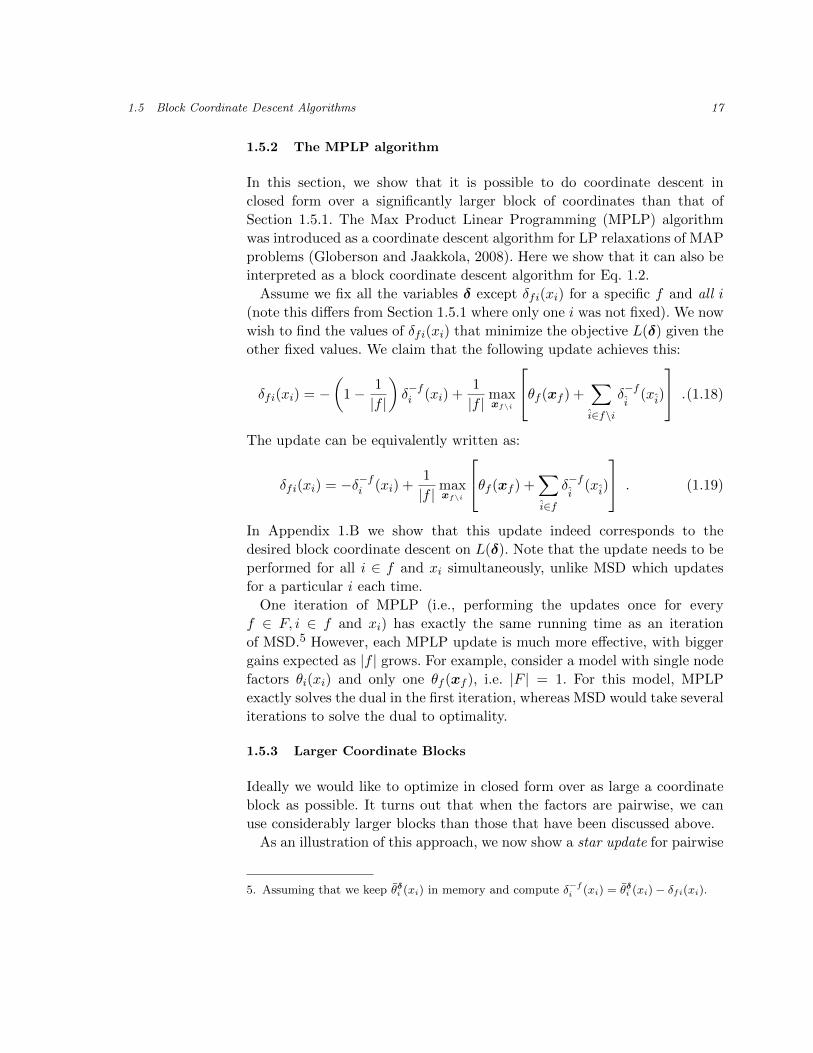
1.5 Block Coordinate Descent Algorithms 17
1.5.2 The MPLP algorithm
In this section, we show that it is possible to do coordinate descent in
closed form over a significantly larger block of coordinates than that of
Section 1.5.1. The Max Product Linear Programming (MPLP) algorithm
was introduced as a coordinate descent algorithm for LP relaxations of MAP
problems (Globerson and Jaakkola, 2008). Here we show that it can also be
interpreted as a block coordinate descent algorithm for Eq. 1.2.
Assume we fix all the variables δ except δfi(xi) for a specific f and all i
(note this differs from Section 1.5.1 where only one i was not fixed). We now
wish to find the values of δfi(xi) that minimize the objective L(δ) given the
other fixed values. We claim that the following update achieves this:
δfi(xi) = −(
1− 1
|f |
)δ−fi (xi) +
1
|f | maxxf\i
θf (xf ) +∑i∈f\i
δ−fi
(xi)
.(1.18)
The update can be equivalently written as:
δfi(xi) = −δ−fi (xi) +1
|f | maxxf\i
θf (xf ) +∑i∈f
δ−fi
(xi)
. (1.19)
In Appendix 1.B we show that this update indeed corresponds to the
desired block coordinate descent on L(δ). Note that the update needs to be
performed for all i ∈ f and xi simultaneously, unlike MSD which updates
for a particular i each time.
One iteration of MPLP (i.e., performing the updates once for every
f ∈ F, i ∈ f and xi) has exactly the same running time as an iteration
of MSD.5 However, each MPLP update is much more effective, with bigger
gains expected as |f | grows. For example, consider a model with single node
factors θi(xi) and only one θf (xf ), i.e. |F | = 1. For this model, MPLP
exactly solves the dual in the first iteration, whereas MSD would take several
iterations to solve the dual to optimality.
1.5.3 Larger Coordinate Blocks
Ideally we would like to optimize in closed form over as large a coordinate
block as possible. It turns out that when the factors are pairwise, we can
use considerably larger blocks than those that have been discussed above.
As an illustration of this approach, we now show a star update for pairwise
5. Assuming that we keep θδi (xi) in memory and compute δ−fi (xi) = θδi (xi)− δfi(xi).

18 Introduction to Dual Decomposition for Inference
models (Globerson and Jaakkola, 2008). Consider a model where factors
correspond to pairs of variables, so that the elements of F are of the
form {i, j}. Now, consider a block coordinate descent approach where the
free coordinates are δ{i,j}j(xj), δ{i,j}i(xi) for a given i and all its neighbors
j ∈ N(i). Although it is non-trivial to derive, we show in Appendix 1.C that
a closed form update for these coordinates exists. The free coordinates that
minimize the objective L(δ) are given by:6
δ{i,j}i(xi) = − 1
1 +Niγi(xi) + γji(xi) (1.20)
δ{i,j}j(xj) = −12δ−ij (xj) + 1
2 maxxi
[θij(xi, xj) +
2
1 +Niγi(xi)− γji(xi)
]where we define δ−ij (xj) = θj(xj) +
∑k∈N(j)\i δ{k,j}j(xj) and:
γji(xi) = maxxj
[θij(xi, xj) + δ−ij (xj)
]γi(xi) = θi(xi) +
∑j∈N(i)
γji(xi)
where Ni = |N(i)| is the number of neighbors of node i in the pairwise
model. For a given node i, the update needs to be performed for all factors
{i, j}, xi, and xj simultaneously, where j ∈ N(i).
Often a closed form update is not possible but one can still efficiently
compute the updates. For example, Sontag and Jaakkola (2009) give a
linear time algorithm for coordinate descent in pairwise models using blocks
corresponding to the edges of a tree-structured graph.
1.5.4 Efficiently Computing the Updates
Recall that the subgradient method only needs to solve one maximization per
subproblem to perform the subgradient update (see Eq. 1.15). We showed in
Section 1.4.2 that these can be solved efficiently for a large number of sparse
factors, even though the factors may involve a large number of variables.
Consider the MPLP update given in Eq. 1.16. To perform the updates
one must compute max-marginals for each subproblem, i.e. the value of the
optimal assignment after fixing each variable (individually) to one of its
6. The star update that appeared in Globerson and Jaakkola (2008) (under the nameNMPLP) had an error. This is the correct version.

1.5 Block Coordinate Descent Algorithms 19
states. Specifically, for every f, i and xi, we must compute:
maxxf\i
h(xf\i, xi), h(xf ) = θf (xf ) +∑i∈f
δ−fi
(xi) .
Often this can be done with the same running time that it takes to find the
maximizing assignment, i.e. maxxfh(xf ).7 For example, if the subproblem
is a tree structure, then with just two passes – propagating max-product
messages from the leaves to the root, and then from the root back to the
leaves – we can compute the max-marginals. Tarlow et al. (2010) show how
max-marginals can be efficiently computed for factors enforcing cardinality
and order constraints, and Duchi et al. (2007) show how to do this for
matchings. In all of these cases, one iteration of MPLP has the same running
time as one iteration of the subgradient method.
However, for some problems, computing the max-marginals can take
longer. For example, it is not clear how to efficiently compute max-marginals
for the factor θ1(x) which enforced acyclicity in the non-projective depen-
dency problem. The weight for the edge corresponding to xi is δ−1i (0) −δ−1i (1). The computational problem is to find, for each edge, the weight of
the minimum directed spanning tree (MST) if we force it to include this
edge (xi = 1) and if we force it not to include this edge (xi = 0).8 We
could compute the max-marginals by solving 2|V | separate directed MST
problems, but this would increase the overall running time of each iteration.
Thus, it is possible that the subgradient approach is better suited here.
1.5.5 Empirical Comparison of the Algorithms
All the algorithms described in this section minimize L(δ), but do so
via different coordinate blocks. How do these algorithms compare to one
another? One criterion is the number of coordinates per block. The more
coordinates we optimize in closed form, the faster we would expect our
algorithm to make progress. Thus, we would expect the MPLP updates
given in Section 1.5.2 to minimize L(δ) in fewer iterations than the MSD
updates from Section 1.5.1, since the former optimizes over more coordinates
simultaneously. Comparing the star update from Section 1.5.3 to MPLP with
edge updates is a bit more delicate since, in the former, the coordinate blocks
overlap. Thus, we may be doing redundant computations in the star update.
On the other hand, it does provide a closed-form update over larger blocks
7. To perform the updates we need only the optimal value, not the maximizing assignment.8. The corresponding max-marginal is the MST’s weight plus the constant −
∑i∈f δ
−1i (0).

20 Introduction to Dual Decomposition for Inference
0 10 20 30 40 50 6046
47
48
49
50
51
52
Iteration
Ob
jective
MSD
MSD++
MPLP
Star
Figure 1.5: Comparison of three coordinate descent algorithms on a 10×10two dimensional Ising grid. The dual objective L(δ) is shown as a function ofiteration number. We multiplied the number of iterations for the star updateby two, since each edge variable is updated twice.
and thus may result in faster convergence.
To assess the difference between the algorithms, we test them on a pairwise
model with binary variables. The graph structure is a two dimensional 10×10
grid and the interactions are Ising (see Globerson and Jaakkola, 2008, for a
similar experimental setup). We compare three algorithms:
MSD - At each iteration, for each edge, updates the message from the
edge to one of its endpoints (i.e., δ{i,j}i(xi) for all xi), and then updates the
message from the edge to its other endpoint.
MPLP - At each iteration, for each edge, updates the messages from the
edge to both of its endpoints (i.e., δ{i,j}i(xi) and δ{i,j}j(xj), for all xi, xj).
Star update - At each iteration, for each node i, updates the messages
from all edges incident on i to both of their endpoints (i.e., δ{i,j}i(xi) and
δ{i,j}j(xj) for all j ∈ N(i), xi, xj).
MSD++ - See Section 1.5.6 below.
The running time per iteration of MSD and MPLP are identical. We let
each iteration of the star update correspond to two iterations of the edge
updates to make the running times comparable.
Results for a model with random parameters are shown in Fig. 1.5, and

1.5 Block Coordinate Descent Algorithms 21
are representative of what we found across a range of model parameters.
The results verify the arguments made above: MPLP is considerably faster
than MSD, and the star update is somewhat faster than MPLP.
1.5.6 What makes MPLP faster than MSD?
It is clear that MPLP uses a larger block size than MSD. However, the two
algorithms also use different equalization strategies, which we will show is
just as important. We illustrate this difference by giving a new algorithm,
MSD++, which uses the same block size as MPLP, but an equalization
method that is more similar to MSD’s.
For a given factor f , assume all δ variables are fixed except δfi(xi) for all
i ∈ f and xi (as in MPLP). We would like to minimize L(δ) with respect to
the free variables. The part of the objective L(δ) that depends on the free
variables is
L(δ) =∑i∈f
maxxi
θδi (xi) + maxxf
θδf (xf ) ,
where θ are the reparameterizations defined in Eq. 1.6.
The MPLP update can be shown to give a δt+1 such that L(δt+1) =
maxxfhδ
t
(xf ), where hδt
(xf ) =∑
i∈f θδti (xi) + θδ
t
f (xf ). However, there are
many possible choices for δt+1 that would achieve the same decrease in the
dual objective. In particular, for any choice of non-negative weights αf , αi
for i ∈ f such that αf +∑
i∈f αi = 1, we can choose δt+1 so that
θδt+1
i (xi) = αi ·maxxf\i
hδt
(xf ) ∀i ∈ f,
θδt+1
f (xf ) = hδt
(xf )−∑i∈f
αi ·maxxf\i
hδt
(xi, xf\i).
Thus, we have that maxxiθδ
t+1
i (xi) = αi·maxxfhδ
t
(xf ) and maxxfθδ
t+1
f (xf )
= αf ·maxxfhδ
t
(xf ). All of these statements can be proved using arguments
analogous to those given in Appendix 1.B.
The MPLP algorithm corresponds to the choice αf = 0, αi = 1|f | for
i ∈ f . The reparameterization results in as much of hδt
(xf ) being pushed
to the single node terms θδt+1
i (xi) as possible. Thus, subsequent updates for
other factors that share variables with f will be affected by this update as
much as possible. Intuitively, this increases the amount of communication
between the subproblems. MPLP’s dual optimal fixed points will have
maxxiθδi (xi) = L(δ)
|V | for all i, and maxxfθδf (xf ) = 0 for all f ∈ F .
In contrast, each MSD update to δfi(xi) divides the objective equally
between the factor term and the node term (see Appendix 1.A). As a

22 Introduction to Dual Decomposition for Inference
result, MSD’s dual optimal fixed points have maxxiθδi (xi) = maxxf
θδf (xf ) =L(δ)|V |+|F | for all i ∈ V and f ∈ F . Consider the alternative block coordinate
descent update given by
δfi(xi) =−|f ||f |+ 1
δ−fi (xi) +1
|f |+ 1maxxf\i
θf (xf ) +∑i∈f\i
δ−fi
(xi)
(1.21)
for all i ∈ f and xi simultaneously. This update, which we call MSD++,
corresponds to the choice αi = αf = 1|f |+1 , and has similar fixed points.
We show in Fig. 1.5 that MSD++ is only slightly faster than MSD, despite
it using a block size that is the same as MPLP. This suggests that it is
MPLP’s choice of equalization method (i.e., the αi’s) that provides the
substantial improvements over MSD, not simply the choice of block size.
As αf → 1, the number of iterations required to solve the dual to optimality
increases even further. The extreme case, αf = 1, although still a valid block
coordinate descent step, gets stuck after the first iteration.
1.5.7 Convergence of Dual Coordinate Descent
Although coordinate descent algorithms decrease the dual objective at every
iteration, they are not generally guaranteed to converge to the dual opti-
mum. The reason is that although the dual objective L(δ) is convex, it is
not strictly convex. This implies that the minimizing coordinate value may
not be unique, and thus convergence guarantees for coordinate descent algo-
rithms do not hold (Bertsekas, 1995). Interestingly, for pairwise MRFs with
binary variables, the fixed points of the coordinate descent algorithms do
correspond to global optima (Kolmogorov and Wainwright, 2005; Globerson
and Jaakkola, 2008).
One strategy to avoid the above problem is to replace the max function
in the objective of Eq. 1.2 with a soft-max function (e.g., see Johnson,
2008; Hazan and Shashua, 2010) which is smooth and strictly convex. As a
result, coordinate descent converges globally.9 An alternative approach are
the auction algorithms proposed by Bertsekas (1992). However, currently
there does not seem to be a coordinate descent approach to Eq. 1.2 that is
guaranteed to converge globally for general problems.
9. To solve the original dual, the soft-max needs to be gradually changed to the true max.

1.6 Relations to Linear Programming Relaxations 23
1.6 Relations to Linear Programming Relaxations
Linear programming relaxations are a popular approach to approximating
combinatorial optimization problems. One of these relaxations is in fact
well-known to be equivalent to the dual decomposition approach discussed
in this paper (Schlesinger, 1976; Guignard and Kim, 1987; Komodakis et al.,
2010; Wainwright et al., 2005; Werner, 2007). In this section we describe the
corresponding LP relaxation.
We obtain a relaxation of the discrete optimization problem given in
Eq. 1.1 by replacing it with the following linear program:
maxµ∈ML
{∑f
∑xf
θf (xf )µf (xf ) +∑i
∑xi
θi(xi)µi(xi)
}(1.22)
where the local marginal polytope ML enforces that {µi(xi),∀xi} and
{µf (xf ), ∀xf} correspond to valid (local) probability distributions and that,
for each factor f , µf (xf ) is consistent with µi(xi) for all i ∈ f, xi:
ML =
{µ ≥ 0 :
∑xf\i
µf (xf ) = µi(xi) ∀f, i ∈ f, xi∑xiµi(xi) = 1 ∀i
}(1.23)
Standard duality transformations can be used to show that the convex
dual of the LP relaxation (Eq. 1.22) is the Lagrangian relaxation (Eq. 1.2).
The integral vertices of the local marginal polytope (i.e., µ such that
µi(xi) ∈ {0, 1}) can be shown to correspond 1-to-1 with assignments x
to the variables of the graphical model. The local marginal polytope also
has fractional vertices that do not correspond to any global assignment
(Wainwright and Jordan, 2008). Since the relaxation optimizes over this
larger space, the value of the LP solution always upper bounds the value
of the MAP assignment. We call the relaxation tight for an instance if the
optimum of the LP has the same value as the MAP assignment.
The connection to LP relaxations is important for a number of reasons.
First, it shows how the algorithms discussed in this paper apply equally
to dual decomposition and linear programming relaxations for the MAP
problem. Second, it allows us to understand when two different dual decom-
positions are equivalent to each other in the sense that, for all instances,
the Lagrangian relaxation provides the same upper bound (at optimality).
Realizing that two formulations are equivalent allows us to attribute differ-
ences in empirical results to the algorithms used to optimize the duals, not
the tightness of the LP relaxation.
The third reason why the connection to LP relaxations is important is
24 Introduction to Dual Decomposition for Inference
because it allows us to tighten the relaxation by adding valid constraints that
are guaranteed not to cut off any integer solutions. The dual decomposition
that we introduced in Section 1.3 used only single node intersection sets,
enforcing that the subproblems are consistent with one another on the
individual variables. To obtain tighter LP relaxations, we typically have
to use larger intersection sets along with the new constraints.10 Although
further discussion of this is beyond the scope of this chapter, details can be
found in Sontag (2010) and Werner (2008).
1.7 Decoding: Finding the MAP Assignment
Thus far, we have discussed how the subgradient method and block coordi-
nate descent can be used to solve the Lagrangian relaxation. Although this
provides an upper bound on the value of the MAP assignment, for most
inference problems we actually want to find the assignment itself. We sug-
gested in Fig. 1.4 one simple way to find an assignment from the dual beliefs,
by locally decoding the single node reparameterizations:
xi ← argmaxxi
θδi (xi). (1.24)
The node terms θδi (xi) may not have a unique maximum. However, when
they do have a unique maximum, we say that δ is locally decodable to x. This
section addresses the important question of when this and related approaches
will succeed at finding the MAP assignment. Proofs are given in Appendix
1.D.
Before the dual is solved (close) to optimality, it is typically not possible
to give guarantees as to how good an assignment will be found by this
local decoding scheme. However, once the algorithms have solved the dual
to optimality, if the solution is locally decodable to x, then x is both the
MAP assignment and the only LP solution, as stated in the next theorem.
Theorem 1.2. If a dual optimal δ∗ is locally decodable to x∗, then the LP
relaxation has a unique solution and it is x∗.
Thus, this result gives a strong necessary condition for when locally decod-
ing the dual solution can find the MAP assignment – only when the LP
relaxation is tight, the MAP assignment is unique, and there are not any
optimal fractional solutions.11
10. Globerson and Jaakkola (2008) give the MPLP updates for larger intersection sets.11. An alternative way to find the MAP assignment in this setting would be to directly

1.7 Decoding: Finding the MAP Assignment 25
A natural question is whether this assumption, i.e. that the LP relaxation
has a unique solution and it is integral, is sufficient for a dual solution to be
locally decodable. As we illustrate later, in general the answer is no, as not
all dual solutions are locally decodable. We are, however, guaranteed that
one exists:
Theorem 1.3. If the LP relaxation has a unique solution and it is integral,
there exists a dual optimal δ∗ that is locally decodable.
Ideally, our algorithms would be guaranteed to find such a locally decod-
able dual solution. We show in Section 1.7.1 that the subgradient method is
indeed guaranteed to find a locally decodable solution under this assump-
tion. For coordinate descent methods there do exist cases where a locally
decodable solution may not be found. However, in practice this is often not
a problem, and there are classes of graphical models where locally decodable
solutions are guaranteed to be found (see Section 1.7.2).
Rather than locally decoding an assignment, we could try searching for
a global assignment x∗ which maximizes each of the local subproblems.
We showed in Theorem 1.1 that such an agreeing assignment would be a
MAP assignment, and its existence would imply that the LP relaxation is
tight. Thus, the LP relaxation being tight is a necessary requirement for this
strategy to succeed. For pairwise models with binary variables, an agreeing
assignment can be found in linear time when one exists (Johnson, 2008).
However, this does not extend to larger factors or non-binary variables:
Theorem 1.4. Finding an agreeing assignment is NP-complete even when
the LP relaxation is tight and the MAP assignment is unique.
The construction in the above theorem uses a model where the optimum
of the LP relaxation is not unique; although there may be a unique MAP
assignment, there are also fractional vertices that have the same optimal
value. When the LP has a unique and integral optimum, the decoding
problem is no longer hard (e.g., it can be solved by optimizing an LP). Thus,
asking that the LP relaxation have a unique solution that is integral seems
to be a very reasonable assumption for a decoding method to succeed. When
the LP relaxation does not have a unique solution, a possible remedy is to
perturb the objective function by adding a small (in magnitude) random
vector. If the LP relaxation is not tight, we can attempt to tighten the
relaxation, e.g. using the approaches discussed in Sontag et al. (2008).
solve the LP relaxation using a generic LP solver. However, recall that we use dualdecomposition for reasons of computational efficiency.

26 Introduction to Dual Decomposition for Inference
1.7.1 Subgradient Method
The problem of recovering a primal solution (i.e., a solution to the LP re-
laxation given in Eq. 1.22) when solving a Lagrangian relaxation using sub-
gradient methods has been well-studied (e.g., see Anstreicher and Wolsey,
2009; Nedic and Ozdaglar, 2008; Shor et al., 1985). We next describe one
such approach (the simplest) and discuss its implications for finding the
MAP assignment from the dual solution.
Given the current dual variables δt, define the following indicator func-
tions for a maximizing assignment of the subproblems: µtf (xf ) = 1[xf =
argmaxxfθδ
t
f (xf )], and µti(xi) = 1[xi = argmaxxiθδ
t
i (xi)]. When the maxi-
mum is not unique, choose any one of the maximizing assignments.
Next, consider the average of these indicator functions across all subgra-
dient iterations:
µf (xf ) =1
T
T∑t=1
µtf (xf )
µi(xi) =1
T
T∑t=1
µti(xi).
For many common choices of step-sizes, the estimate µ can be shown to
converge to a solution of the LP relaxation given in Eq. 1.22, as T →∞.
When the LP relaxation has a unique solution and it is integral, then µ
is guaranteed converge to the unique MAP assignment. In particular, this
implies that there must exist a subgradient iteration when µt corresponds
to the MAP assignment. At this iteration the subgradient is zero, and we
obtain a certificate of optimality by Theorem 1.1. When the LP relaxation is
not tight, recovering a primal solution may be helpful for finding additional
constraints to use in tightening the relaxation.
1.7.2 Coordinate Descent
As we mentioned in Section 1.5, the coordinate descent algorithms, while
always providing a monotonic improvement in the dual objective, are not
in general guaranteed to solve the Lagrangian relaxation to optimality.
However, for some graphical models, such as pairwise models with binary
variables, fixed points of the coordinate descent algorithms can be used to
construct a solution to the LP relaxation (Kolmogorov and Wainwright,
2005; Globerson and Jaakkola, 2008). Thus, for these graphical models, all
fixed points of the algorithms are dual optimal.
We additionally show that, when the LP relaxation has a unique solution

1.8 Discussion 27
that is integral, then the fixed point must be locally decodable to the MAP
assignment. On the other hand, for more general graphical models, there do
exist degenerate cases when a fixed point of the coordinate descent algorithm
is not locally decodable, even if it corresponds to a dual solution.
Theorem 1.5. Suppose the LP relaxation has a unique solution and it is
integral.12 Then the following holds:
1. For binary pairwise MRFs, fixed points of the coordinate descent algo-
rithms are locally decodable to x∗.
2. For pairwise tree-structured MRFs, fixed points of the coordinate descent
algorithms are locally decodable to x∗.
3. There exist non-binary pairwise MRFs with cycles and dual optimal fixed
points of the coordinate descent algorithms that are not locally decodable.
The second result can be generalized to graphs with a single cycle. Despite
the theoretical difficulty hinted at in the third result, empirically we have
found that – when the LP relaxation has a unique solution that is integral –
local decoding nearly always succeeds at finding the MAP assignment, when
used with the coordinate descent algorithms (Sontag et al., 2008).
1.8 Discussion
The dual decomposition formulation that we introduced in this chapter is
applicable whenever one can break an optimization problem into smaller
subproblems that can be solved exactly using combinatorial algorithms. The
dual objective is particularly simple, consisting of a sum of maximizations
over the individual subproblems, and provides an upper bound on the value
of the MAP assignment. Minimizing the Lagrangian relaxation makes this
bound tighter by pushing the subproblems to agree with one another on
their maximizing assignment. If we succeed in finding an assignment that
maximizes each of the individual subproblems, then this assignment is the
MAP assignment and the dual provides a certificate of optimality. Even
when not exact, the upper bound provided by the dual can be extremely
valuable when used together with a branch-and-bound procedure to find the
MAP assignment (Geoffrion, 1974).
We described both subgradient methods and block coordinate algorithms
for minimizing the Lagrangian relaxation. Both are notable for their simplic-
12. Note that this implies that the MAP assignment x∗ is unique.

28 Introduction to Dual Decomposition for Inference
ity and their effectiveness at solving real-world inference problems. A natu-
ral question is how to choose between the two for a specific problem. This
question has been of continual debate since the early work on Lagrangian
relaxations (see Guignard, 2003, for a review).
Each approach has its advantages and disadvantages. The subgradient
method is guaranteed to converge, but does not monotonically decrease the
dual, and requires a delicate choice of step size. The coordinate descent
algorithms are typically much faster at minimizing the dual, especially in
the initial iterations, and are also monotonic. However, to perform each
update one must compute max-marginals, and this may be impractical for
some applications. We presented several coordinate update schemes. These
vary both in the coordinates that they choose to minimize in each update,
and in the way this minimization is performed. MPLP appears to be the
best general choice.
It may be advantageous to use the two approaches together. For example,
one could first use coordinate descent and then, when the algorithm is close
to convergence, use the subgradient method to ensure global optimality.
Another possibility is to alternate between the updates, as in the spacer
step approach in optimization (see Bertsekas, 1995).
There are often many different ways to decompose a problem when
applying dual decomposition. For example, in this chapter we suggested
using a decomposition for pairwise models that uses one subproblem per
edge. An alternative decomposition is to use a set of spanning trees that
together cover all of the edge potentials (Wainwright et al., 2005). Still
another approach is to, before constructing the decomposition, “split” some
of the variables and introduce new potentials to enforce equality among all
copies of a variable (Guignard, 2003). Using this technique, Yarkony et al.
(2010) give a decomposition that uses a single tree spanning all of the original
edge potentials. Although in all of these cases the decompositions correspond
to the same LP relaxation, often a different decomposition can result in
tighter or looser bounds being provided by the Lagrangian relaxation.
Dual decomposition methods have a wide range of potential applications in
machine learning and, more broadly, engineering and the sciences. We have
already observed some empirical successes for natural language processing,
computational biology, and machine vision. We expect that as graphical
models become more complex, techniques like the ones discussed in this
chapter will become essential for performing fast and accurate inference.
Acknowledgements We thank Michael Collins, Ce Liu, and the editors
for their very useful feedback, and also to M. Collins for Fig. 1.1. This work
was partly supported by BSF grant 2008303.

1.A Derivation of the Max Sum Diffusion Updates 29
Appendix
1.A Derivation of the Max Sum Diffusion Updates
For a given factor f and variable i assume all δ variables are fixed except
δfi(xi). We would like to minimize L(δ) in Eq. 1.2 w.r.t. the free variables.
Here we prove that the choice of δfi(xi) in Eq. 1.17 corresponds to this
minimization (note that other updates that achieve the same objective are
possible since L(δ) not strictly convex).
The part of the objective L(δ) that depends on the free parameters is:
maxxi
(θi(xi) +
∑f :i∈f
δfi(xi))
+ maxxf
(θf (xf )−
∑i∈f
δf i(xi))
= maxxi
(δfi(xi) + δ−fi (xi)
)+ max
xi
(−δfi(xi) + max
xf\i
[θf (xf )−
∑i∈f\i
δf i(xi)])
≥ maxxi
(δ−fi (xi) + max
xf\i
[θf (xf )−
∑i∈f\i
δf i(xi)])
= maxxi
g(xi).
This lower bound can be achieved by choosing a δfi(xi) such that:
δfi(xi) + δ−fi (xi) = 12g(xi),
−δfi(xi) + maxxf\i
[θf (xf )−
∑i∈f\i
δf i(xi)]
= 12g(xi).
Indeed, the δfi(xi) given by the update in Eq. 1.17 satisfies the above.
1.B Derivation of the MPLP Updates
For a given factor f assume all δ variables are fixed except δfi(xi) for all
i ∈ f . We would like to minimize L(δ) in Eq. 1.2 w.r.t. the free variables.
Here we prove that Eq. 1.18 does this optimally.
The part of the objective L(δ) that depends on the free parameters is:
L(δ) =∑i∈f
maxxi
(θi(xi)+
∑f :i∈f
δf i(xi))
+maxxf
(θf (xf )−
∑i∈f
δfi(xi))
(1.25)
DenoteAi(δ) = maxxi
(θi(xi)+
∑f :i∈f δf i(xi)
)andAf (δ) = maxxf
(θf (xf )−

30 Introduction to Dual Decomposition for Inference
∑i∈f δfi(xi)
). Then it follows that:
L(δ) =∑i∈f
Ai(δ) +Af (δ) ≥ maxxf
(θf (xf ) +
∑i∈f
δ−fi (xi))
= B.
This gives a lower bound B on the minimum of L(δ). We next show that
this lower bound is achieved by the MPLP update in Eq. 1.18. For each of
the terms Ai(δ) we have (after the update):
Ai(δ) = maxxi
1
|f |δ−fi (xi) +
1
|f | maxxf\i
θf (xf ) +∑i∈f\i
δ−fi
(xi)
=
1
|f | maxxf
(θf (xf ) +
∑i∈f
δ−fi (xi))
=B
|f | . (1.26)
The value of Af (δ) after the MPLP update is:
maxxf
(θf (xf ) +
∑i∈f
{ |f | − 1
|f | δ−fi (xi)−1
|f | maxxf\i
[θf (xi, xf ) +
∑i∈f\i
δ−fi
(xi)]})
=1
|f | maxxf
(∑i∈f
{θf (xf ) +
∑i∈f\i
δ−fi
(xi)−maxxf\i
[θf (xi, xf ) +
∑i∈f\i
δ−fi
(xi)]})
≤ 1
|f |∑i∈f
maxxf
(θf (xf ) +
∑i∈f\i
δ−fi
(xi)−maxxf\i
[θf (xi, xf ) +
∑i∈f\i
δ−fi
(xi)])
=1
|f |∑i∈f
maxxi
(maxxf\i
[θf (xf ) +
∑i∈f\i
δ−fi
(xi)]−maxxf\i
[θf (xf ) +
∑i∈f\i
δ−fi
(xi)])
= 0,
where the first equality used∑
i∈f (|f | − 1)δ−fi (xi) =∑
i∈f∑
i∈f\i δ−fi
(xi).
From the above and Eq. 1.26 it follows that L(δ) ≤ B. However, we know
that B is a lower bound on L(δ) so we must have L(δ) = B, implying the
optimality of the MPLP update.
1.C Derivation of the Star Update
The MPLP update gives the closed form solution for block coordinate
descent on coordinates δ{i,j}j(xj) and δ{i,j}i(xi) for a particular {i, j} ∈ F(i.e., an edge update). We now wish to find the update where the free
coordinates are δ{i,j}j(xj), δ{i,j}i(xi) for a fixed i and all j ∈ N(i). One way
to find the optimal coordinates is by iterating the MPLP update for all the

1.D Proofs of the Decoding Results 31
edges in the star until convergence. Notice that δ−ij (xj), γji(xi), and γi(xi)
do not change after each edge update. We solve for δ{i,j}j(xj) and δ{i,j}i(xi)
in terms of these quantities, using fixed point equations for MPLP.
The MPLP edge update for f = {i, j} is given by
δ{i,j}i(xi) = −12δ−ji (xi) + 1
2γji(xi) . (1.27)
Multiplying by 2, and then subtracting δ{i,j}i(xi) from both sides, we obtain
δ{i,j}i(xi) = −δi(xi) + γji(xi) , (1.28)
where we define δi(xi) = θi(xi) +∑
j∈N(i) δ{i,j}i(xi). Summing this over all
neighbors of i, and adding θi(xi) to both sides, we obtain:
δi(xi) = −Niδi(xi) + γi(xi)
δi(xi) =1
1 +Niγi(xi) . (1.29)
Applying Eq. 1.28 and Eq. 1.29, we obtain the following for δ−ji (xi):
δ−ji (xi) = δi(xi)− δ{i,j}i(xi) = 2δi(xi)− γji(xi) =2γi(xi)
1 +Ni− γji(xi) .
Substituting this back into the MPLP update (Eq. 1.27) yields the update
for δ{i,j}i(xi) given in Eq. 1.20. The update for δ{i,j}j(xj) is obtained by
taking the MPLP update and substituting the above expression for δ−ji (xi).
The dual variables given by the star update in Eq. 1.20 can be seen to
be a fixed point of MPLP for all edges in the star. Since any fixed point of
MPLP on a tree is dual optimal (see Section 1.7.2), these updates provide
the optimum for these coordinates.
1.D Proofs of the Decoding Results
Duality in linear programming specifies complementary slackness conditions
that every primal and dual solution must satisfy. In particular, it can be
shown that for any optimal µ∗ for the local LP relaxation given in Eq. 1.22
and any optimal δ∗ for the Lagrangian relaxation minδ L(δ),
µ∗i (xi) > 0 ⇒ θδ∗
i (xi) = maxxi
θδ∗
i (xi), (1.30)
µ∗f (xf ) > 0 ⇒ θδ∗
f (xf ) = maxxf
θδ∗
f (xf ). (1.31)
Proof of Theorem 1.2. Consider any xi 6= x∗i . Since θδ∗
i (xi) < θδ∗
i (x∗i ),
complementary slackness (1.30) implies that µ∗i (xi) = 0 for all optimal µ∗.

32 Introduction to Dual Decomposition for Inference
Thus, the only solution to the LP relaxation corresponds to x∗.
Proof of Theorem 1.3. This follows from strict complementary slackness
(Vanderbei, 2007), which guarantees that a primal-dual pair (µ∗, δ∗) exists
that satisfies the implication in (1.30) both ways. Since the LP relaxation
has only one solution and it corresponds to the MAP assignment, strict
complementary slackness guarantees that such a δ∗ is locally decodable.
Proof of Theorem 1.4. We reduce from 3SAT. First, we encode 3SAT as an
optimization problem of the form given in Eq. 1.1. The variables xi ∈ {0, 1}are the same as in the 3SAT formula. We have one factor θf (xf ) for each
clause f in the formula, defined on the corresponding three variables. θf (xf )
is 0 if the clause is satisfied by xf , and −∞ otherwise. θi(xi) = 0 for all i, xi.
Suppose we could efficiently find an agreeing assignment when one exists.
By Theorem 1.1, this would be a MAP assignment (and the LP relaxation is
tight), which in this case corresponds to a satisfying assignment of the 3SAT
formula. Thus, if we could efficiently find a MAP assignment whenever the
LP relaxation is tight, then we could efficiently solve 3SAT.
Finding the MAP assignment is hard even if it is unique because the
problem of finding a satisfying assignment when we are guaranteed that a
formula has at most one satisfying assignment, called Unique-SAT, is also
NP-hard, under randomized reductions (Valiant and Vazirani, 1985).
For 3SAT, the LP relaxation always has a fractional solution µ ∈ ML
with objective value 0. Thus, by Theorem 1.2 the dual solutions will never
be locally decodable. Let µi(0) = µi(1) = .5 for all i. For each clause f , if
it is satisfied by both x1f = (0, 0, 0) and x2
f = (1, 1, 1), then let µf (x1f ) =
µf (x2f ) = .5 and µf (xf ) = 0 for xf 6= x1
f ,x2f . Otherwise, f must be satisfied
by x1f = (0, 1, 1) and x2
f = (1, 0, 0), so we set µf (x1f ) = µf (x2
f ) = .5.
Proof of Theorem 1.5, part 1. The claim follows from Proposition 4 given
in Globerson and Jaakkola (2008). This result shows how to construct
a fractional primal solution whenever at least one of the nodes i has
θδi (0) = θδi (1), i.e. when δ is not locally decodable. However, this would
contradict our assumption that the LP relaxation has a unique solution and
it is integral. Thus, δ must be locally decodable.
All fixed points of the coordinate descent algorithms can be shown to
satisfy max-consistency. Let Ai consist of all states xi that maximize θδi (xi).
By max-consistency, we mean that for all f ∈ F, i ∈ f , and xi ∈ Ai,
maxxf\i θδf (xf ) = maxxf
θδf (xf ). This is trivial to see for MSD since, at
a fixed point, θδi (xi) = maxxf\i θδf (xf ) ∀f, i ∈ f and xi. Thus, for xi ∈ Ai,
θδi (xi) = maxxfθδf (xf ). Putting these together shows max-consistency.

1.D Proofs of the Decoding Results 33
X1
X2
X3
X4
1 2 3
4
1
1
1
2
2
2
3
3
3 4
4
4
Figure 1.6: Illustration of the parameters of the pairwise MRF that weuse in the proof of Theorem 1.5, part 3. Each node represents a statexi ∈ {1, 2, 3, 4}. An edge between xi and xj signifies that θij(xi, xj) = 0,whereas no edge between xi and xj signifies that θij(xi, xj) = −1.
Proof of Theorem 1.5, part 2. First, construct a reduced pairwise MRF with
potentials θ′ where for each variable i we consider only those states xi that
maximize θδi (xi) (hereafter ignoring the other states). We let θ′ij(xi, xj) = 0 if
xi, xj maximize θδij(xi, xj), and −∞ otherwise. By complementary slackness,
all solutions of the LP relaxation for θ′ are also optimal for θ. By max-
consistency, for every state xi, ∃xj such that θ′(xi, xj) = 0.
Suppose that there exists a vertex i and state x′i where x′i 6= x∗i (that is, δ
is not locally decodable to x∗). Then, by max-consistency we can construct
an assignment (going one edge at a time in the tree rooted at i) x′ 6= x∗ such
that θ′(x′) = 0. This shows that x′ is a MAP assignment for θ. However,
this contradicts the uniqueness of the MAP assignment.
Proof of Theorem 1.5, part 3. Consider a pairwise MRF on four variables
with edges E = {(1, 2), (2, 3), (3, 4), (1, 4), (1, 3)} and where each variable
has four states. Let the parameters θ be as specified in Fig. 1.6, and let the
dual variables δ be identically zero. Since the MAP assignment (xi = 4 for
all i) has value 0 and L(δ) = 0, δ is dual optimal and the LP relaxation is
tight. δ is also a fixed point of the MPLP update given in Eq. 1.18.
What remains is to show that the LP relaxation has a unique solution (i.e.,
xi = 4 for all i). First, note that for any primal optimal µ∗, µ∗ij(xi, xj) must
be 0 whenever θij(xi, xj) = −1. Subject to these constraints, we next show
that µ∗i (xi) must be 0 for all i and xi ∈ {1, 2, 3}. For x ∈ {1, 2, 3}, the local
consistency constraints (see Eq. 1.23) along edges (1, 2), (2, 3) and (3, 4)

34 Introduction to Dual Decomposition for Inference
imply that µ∗1(x) = µ∗12(x, x) = µ∗2(x) = µ∗2,3(x, x) = µ∗3(x) = µ∗3,4(x) =
µ∗4(x). Similarly, the local consistency constraints along edge (1, 3) imply
that µ∗1(1) = µ∗1,3(1, 2) = µ∗3(2) and µ∗1(2) = µ∗1,3(2, 3) = µ∗3(3). Together,
these imply that µ∗i (xi) = a for all i and xi ∈ {1, 2, 3}. Now consider the
local consistency constraints for edge (1, 4). One of the constraints is that
µ∗1(3) = µ∗1,4(3, 3) + µ∗1,4(3, 2) = µ∗4(3) + µ∗4(2). Thus, we must have that
a = 2a, which implies that a = 0.
Note that there do exist locally decodable solutions for the example given
in Fig. 1.6. In particular, consider δ defined as δ{i,j}i(4) = δ{i,j}j(4) = 0 and
δ{i,j}i(x) = δ{i,j}j(x) = ε for x ∈ {1, 2, 3}. When −.5 ≤ ε < 0, δ is dual
optimal, locally decodable, and a fixed point of MPLP.
References
K. M. Anstreicher and L. A. Wolsey. Two “well-known” properties of
subgradient optimization. Math. Program., 120(1):213–220, 2009.
D. P. Bertsekas. Auction algorithms for network flow problems: A tutorial
introduction. Computational Optimization and Applications, 1:7–66, 1992.
D. P. Bertsekas. Nonlinear Programming. Athena Scientific, Belmont, MA,
1995.
J. Duchi, D. Tarlow, G. Elidan, and D. Koller. Using combinatorial optimiza-
tion within max-product belief propagation. In B. Scholkopf, J. Platt, and
T. Hoffman, editors, Advances in Neural Information Processing Systems
19, pages 369–376. MIT Press, 2007.
D. Erlenkotter. A dual-based procedure for uncapacitated facility location.
Operations Research, 26(6):992–1009, 1978.
M. L. Fisher. The lagrangian relaxation method for solving integer program-
ming problems. Management Science, 27(1):1–18, 1981.
A. M. Geoffrion. Lagrangian relaxation for integer programming. Mathe-
matical Programming Study, 2:82–114, 1974.
A. Globerson and T. Jaakkola. Fixing max-product: Convergent message
passing algorithms for MAP LP-relaxations. In J.C. Platt, D. Koller,
Y. Singer, and S. Roweis, editors, Advances in Neural Information Pro-
cessing Systems 20, pages 553–560. MIT Press, Cambridge, MA, 2008.
M. Guignard. Lagrangean relaxation. TOP: An Official Journal of the
Spanish Society of Statistics and Operations Research, 11(2):151–200,
2003.
1.D Proofs of the Decoding Results 35
M. Guignard and S. Kim. Lagrangean decomposition: A model yielding
stronger Lagrangean bounds. Mathematical Programming, 39(2):215–228,
1987.
M. Guignard and M.B. Rosenwein. An application-oriented guide for design-
ing lagrangean dual ascent algorithms. European Journal of Operational
Research, 43(2):197–205, 1989.
R. Gupta, A.A. Diwan, and S. Sarawagi. Efficient inference with cardinality-
based clique potentials. In Proceedings of the 24th International Confer-
ence on Machine learning, pages 329–336, New York, NY, USA, 2007.
ACM.
T. Hazan and A. Shashua. Norm-product belief propagation: Primal-
dual message-passing for approximate inference. IEEE Transactions on
Information Theory (to appear), 2010.
M. Held, P. Wolfe, and H.P. Crowder. Validation of subgradient optimiza-
tion. Mathematical Programming, 6(1):62–88, 1974.
J. Johnson. Convex Relaxation Methods for Graphical Models: Lagrangian
and Maximum Entropy Approaches. PhD thesis, EECS, MIT, 2008.
D. Koller and N. Friedman. Probabilistic Graphical Models: Principles and
Techniques. MIT Press, 2009.
V. Kolmogorov and M.J. Wainwright. On the optimality of tree-reweighted
max-product message-passing. In Proceedings of the 21st Conference on
Uncertainty in Artificial Intelligence, pages 316–323, Arlington, Virginia,
2005. AUAI Press.
N. Komodakis, N. Paragios, and G. Tziritas. MRF energy minimization and
beyond via dual decomposition. IEEE Transactions on Pattern Analysis
and Machine Intelligence (to appear), 2010.
T. Koo, A. M. Rush, M. Collins, T. Jaakkola, and D. Sontag. Dual decom-
position for parsing with non-projective head automata. In Proceedings of
the 2010 Conference on Empirical Methods in Natural Language Process-
ing, 2010.
V. A. Kovalevsky and V. K. Koval. A diffusion algorithm for decreasing
energy of max-sum labeling problem. Glushkov Institute of Cybernetics,
Kiev, USSR. Unpublished, approx. 1975.
S. Lacoste-Julien, B. Taskar, D. Klein, and M. I. Jordan. Word alignment
via quadratic assignment. In Proceedings of the Human Language Tech-
nology Conference of the North American Chapter of the Association of
Computational Linguistics, pages 112–119, 2006.
C. Lemarechal. Lagrangian relaxation. In Computational Combinatorial

36 Introduction to Dual Decomposition for Inference
Optimization, pages 112–156, 2001.
R. McDonald and G. Satta. On the complexity of non-projective data-driven
dependency parsing. In Proceedings of the 10th International Conference
on Parsing Technologies, pages 121–132, Morristown, NJ, USA, 2007.
Association for Computational Linguistics.
R. McDonald, F. Pereira, K. Ribarov, and J. Hajic. Non-projective depen-
dency parsing using spanning tree algorithms. In Proceedings of the confer-
ence on Human Language Technology and Empirical Methods in Natural
Language Processing, pages 523–530, 2005.
A. Nedic and A. Ozdaglar. Approximate primal solutions and rate analysis
for dual subgradient methods. SIAM J. on Optimization, 19(4):1757–1780,
2008.
C. Rother, P. Kohli, W. Feng, and J. Jia. Minimizing sparse higher order en-
ergy functions of discrete variables. Proc. IEEE Conference on Computer
Vision and Pattern Recognition, pages 1382–1389, 2009.
M. I. Schlesinger. Syntactic analysis of two-dimensional visual signals in
noisy conditions. Kibernetika, 4:113–130, 1976.
N. Z. Shor, K. C. Kiwiel, and A. Ruszcaynski. Minimization methods for
non-differentiable functions. Springer-Verlag New York, Inc., New York,
NY, USA, 1985.
D. Sontag. Approximate Inference in Graphical Models using LP Relax-
ations. PhD thesis, Massachusetts Institute of Technology, Department of
Electrical Engineering and Computer Science, 2010.
D. Sontag and T. Jaakkola. Tree block coordinate descent for MAP in
graphical models. In Proceedings of the 12th International Workshop
on Artificial Intelligence and Statistics, volume 9, pages 544–551. JMLR:
W&CP, 2009.
D. Sontag, T. Meltzer, A. Globerson, T. Jaakkola, and Y. Weiss. Tightening
LP relaxations for MAP using message passing. In Proceedings of the
24th Conference on Uncertainty in Artificial Intelligence, pages 503–510,
Arlington, Virginia, 2008. AUAI Press.
D. Tarlow, I. Givoni, and R. Zemel. Hop-map: Efficient message passing with
high order potentials. In Proceedings of the 13th International Conference
on Artificial Intelligence and Statistics, volume 9, pages 812–819. JMLR:
W&CP, 2010.
L. G. Valiant and V. V. Vazirani. NP is as easy as detecting unique solutions.
In Proceedings of the seventeenth annual ACM symposium on Theory of
computing, pages 458–463, New York, NY, USA, 1985. ACM.

1.D Proofs of the Decoding Results 37
R.J. Vanderbei. Linear Programming: Foundations and Extensions.
Springer, 3rd edition, 2007.
M. Wainwright and M. I. Jordan. Graphical Models, Exponential Families,
and Variational Inference. Now Publishers Inc., Hanover, MA, USA, 2008.
M. Wainwright, T. Jaakkola, and A. Willsky. Tree-based reparameterization
framework for analysis of sum-product and related algorithms. IEEE
Transactions on Information Theory, 49(5):1120–1146, 2003.
M. Wainwright, T. Jaakkola, and A. Willsky. MAP estimation via agreement
on trees: message-passing and linear programming. IEEE Transactions on
Information Theory, 51(11):3697–3717, 2005.
Y. Weiss, C. Yanover, and T. Meltzer. MAP estimation, linear programming
and belief propagation with convex free energies. In Proceedings of the
23rd Conference on Uncertainty in Artificial Intelligence, pages 416–425,
Arlington, Virginia, 2007. AUAI Press.
T. Werner. A linear programming approach to max-sum problem: A review.
IEEE Transactions on Pattern Analysis and Machine Intelligence, 29(7):
1165–1179, 2007.
T. Werner. High-arity interactions, polyhedral relaxations, and cutting plane
algorithm for soft constraint optimisation (MAP-MRF). In CVPR, 2008.
C. Yanover, T. Meltzer, and Y. Weiss. Linear programming relaxations and
belief propagation – an empirical study. Journal of Machine Learning
Research, 7:1887–1907, 2006.
C. Yanover, O. Schueler-Furman, and Y. Weiss. Minimizing and learning
energy functions for side-chain prediction. Journal of Computational
Biology, 15(7):899–911, 2008.
J. Yarkony, C. Fowlkes, and A. Ihler. Covering trees and lower-bounds on
quadratic assignment. In Proc. IEEE Conference on Computer Vision
and Pattern Recognition, 2010.
Top Related