


Languages
Pages
Legal

1GSCM Carl M. Briggs Ph.D.
Network Design in an Uncertain Environment
August 24, 2006 Briggs Session 2
www.kelley.iu.edu/briggsc/e730_lect2.ppt
222GSCM Carl M. Briggs Ph.D. E730 Global Supply Chain Management Program
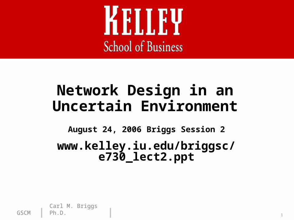
Outline
• Review and work on Sportsstuff.com
• Discuss the use of DCF as a supply chain metric
• Discuss impact of uncertainty on network design decisions
• Review for exam

3GSCM Carl M. Briggs Ph.D.
Review

6GSCM Carl M. Briggs Ph.D.
Network Design Under Uncertainty
777GSCM Carl M. Briggs Ph.D. E730 Global Supply Chain Management Program
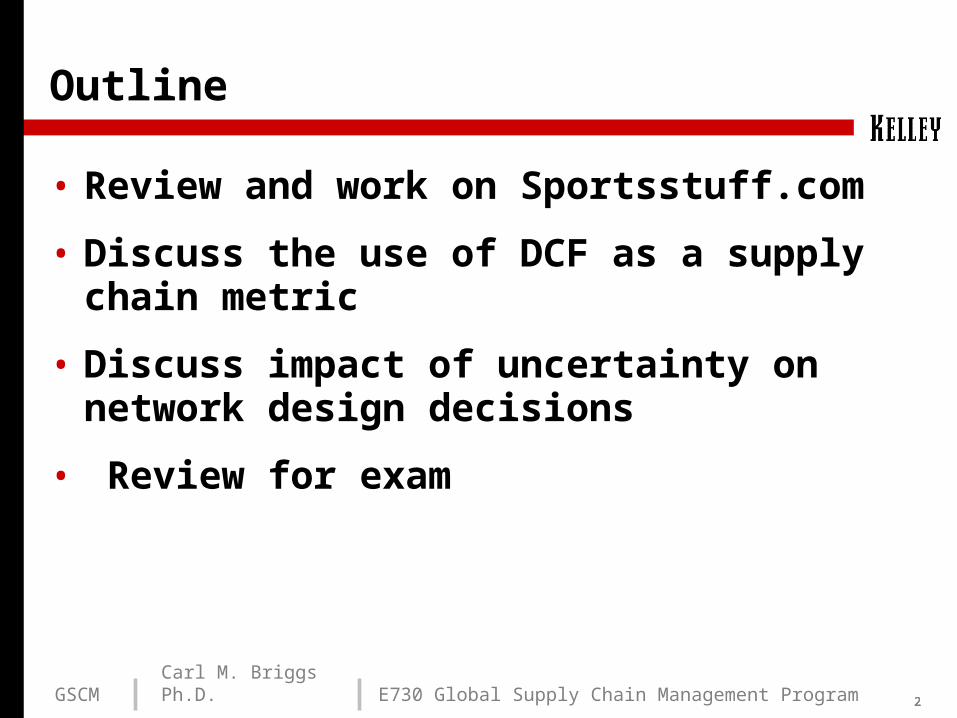
The Impact of Uncertaintyon Network Design
• Supply chain design decisions cannot be easily changed in the short-term.
• There will be a good deal of uncertainty in demand, prices, exchange rates, and the competitive market over the lifetime of a supply chain network.
• Therefore, building flexibility into supply chain operations allows the supply chain to deal with uncertainty in a manner that will maximize profits
888GSCM Carl M. Briggs Ph.D. E730 Global Supply Chain Management Program
Discounted Cash Flow Analysis (DCF)
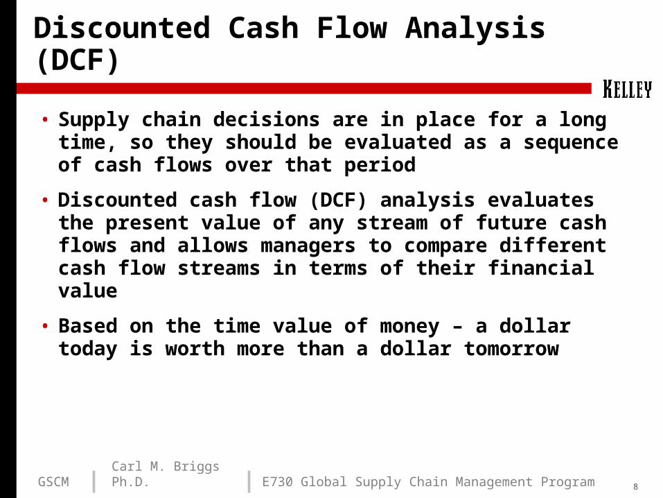
• Supply chain decisions are in place for a long time, so they should be evaluated as a sequence of cash flows over that period
• Discounted cash flow (DCF) analysis evaluates the present value of any stream of future cash flows and allows managers to compare different cash flow streams in terms of their financial value
• Based on the time value of money – a dollar today is worth more than a dollar tomorrow

999GSCM Carl M. Briggs Ph.D. E730 Global Supply Chain Management Program
Discounted Cash Flow Analysis
return of rate
flowscash of stream thisof luepresent vanet the
periods Tover flowscash of stream a is ,...,,
where
1
1
1
1factor Discount
10
10
k
NPV
CCC
Ck
CNPV
k
T
T
tt
t
• Compare NPV of different supply chain design options
• The option with the highest NPV will provide the greatest financial return
101010GSCM Carl M. Briggs Ph.D. E730 Global Supply Chain Management Program
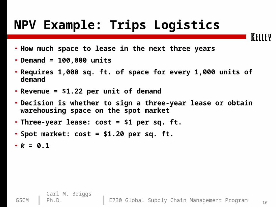
NPV Example: Trips Logistics
• How much space to lease in the next three years
• Demand = 100,000 units
• Requires 1,000 sq. ft. of space for every 1,000 units of demand
• Revenue = $1.22 per unit of demand
• Decision is whether to sign a three-year lease or obtain warehousing space on the spot market
• Three-year lease: cost = $1 per sq. ft.
• Spot market: cost = $1.20 per sq. ft.
• k = 0.1
111111GSCM Carl M. Briggs Ph.D. E730 Global Supply Chain Management Program
NPV Example: Trips Logistics
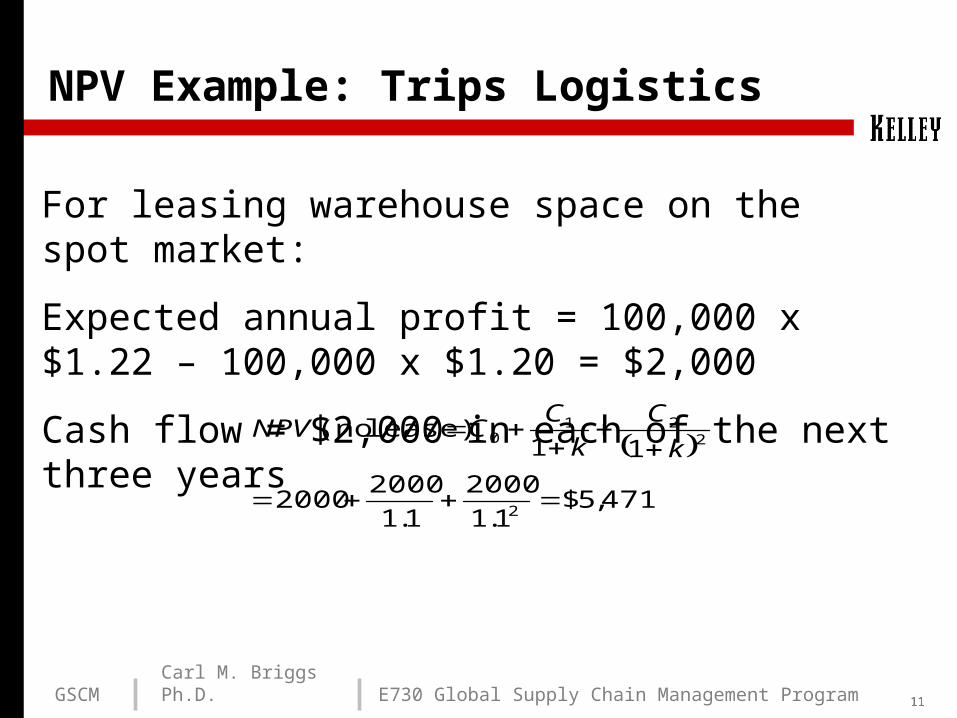
For leasing warehouse space on the spot market:
Expected annual profit = 100,000 x $1.22 – 100,000 x $1.20 = $2,000
Cash flow = $2,000 in each of the next three years
471,5$1.1
2000
1.1
20002000
11lease) (no
2
221
0
k
C
k
CCNPV
121212GSCM Carl M. Briggs Ph.D. E730 Global Supply Chain Management Program
NPV Example: Trips Logistics
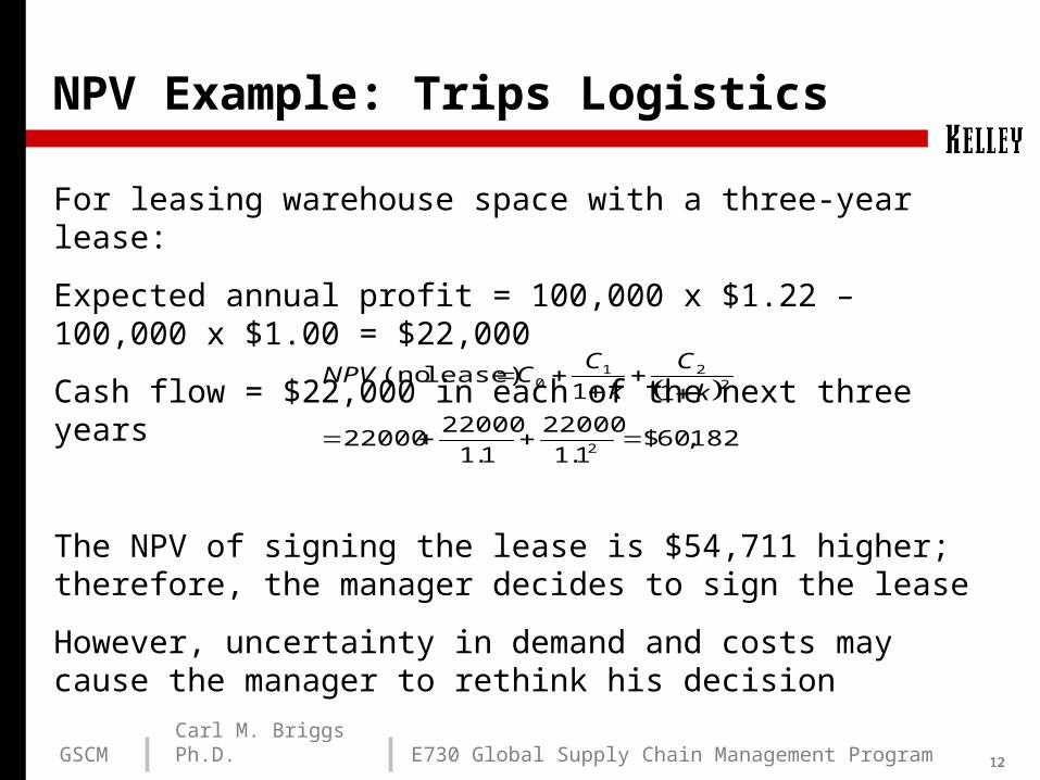
For leasing warehouse space with a three-year lease:
Expected annual profit = 100,000 x $1.22 – 100,000 x $1.00 = $22,000
Cash flow = $22,000 in each of the next three years
182,60$1.1
22000
1.1
2200022000
11lease) (no
2
221
0
k
C
k
CCNPV
The NPV of signing the lease is $54,711 higher; therefore, the manager decides to sign the lease
However, uncertainty in demand and costs may cause the manager to rethink his decision
131313GSCM Carl M. Briggs Ph.D. E730 Global Supply Chain Management Program
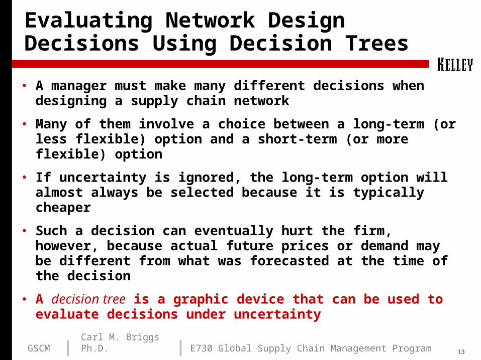
Evaluating Network Design Decisions Using Decision Trees
• A manager must make many different decisions when designing a supply chain network
• Many of them involve a choice between a long-term (or less flexible) option and a short-term (or more flexible) option
• If uncertainty is ignored, the long-term option will almost always be selected because it is typically cheaper
• Such a decision can eventually hurt the firm, however, because actual future prices or demand may be different from what was forecasted at the time of the decision
• A decision tree is a graphic device that can be used to evaluate decisions under uncertainty

141414GSCM Carl M. Briggs Ph.D. E730 Global Supply Chain Management Program
Decision Tree Methodology
1. Identify the duration of each period (month, quarter, etc.) and the number of periods T over the which the decision is to be evaluated.
2. Identify factors such as demand, price, and exchange rate, whose fluctuation will be considered over the next T periods.
3. Identify representations of uncertainty for each factor; that is, determine what distribution to use to model the uncertainty.
4. Identify the periodic discount rate k for each period.
5. Represent the decision tree with defined states in each period, as well as the transition probabilities between states in successive periods.
6. Starting at period T, work back to period 0, identifying the optimal decision and the expected cash flows at each step. Expected cash flows at each state in a given period should be discounted back when included in the previous period.
151515GSCM Carl M. Briggs Ph.D. E730 Global Supply Chain Management Program
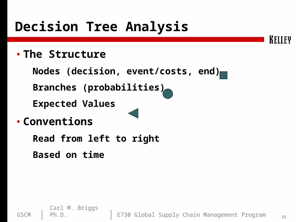
Decision Tree Analysis
• The Structure
Nodes (decision, event/costs, end)
Branches (probabilities)
Expected Values
• Conventions
Read from left to right
Based on time
161616GSCM Carl M. Briggs Ph.D. E730 Global Supply Chain Management Program
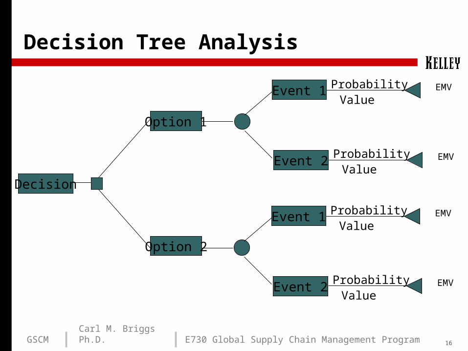
Decision Tree Analysis
Decision
Option 1
Option 2
Event 1
Event 2
EMVProbabilityValue
ProbabilityValue
EMV
Event 1
Event 2
ProbabilityValue
EMV
ProbabilityValue
EMV
171717GSCM Carl M. Briggs Ph.D. E730 Global Supply Chain Management Program
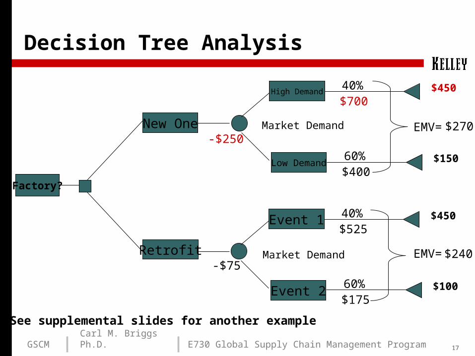
Decision Tree Analysis
Factory?
New One
Retrofit
40%
60%
$700
$400
$450
$150
-$250
$450
$100
-$75
High Demand
Low Demand
Market Demand EMV=
Event 1
Event 2
40%$525
60%$175
Market Demand EMV=
$270
$240
See supplemental slides for another example
18GSCM Carl M. Briggs Ph.D.
Leading a Supply Chain Turnaround

191919GSCM Carl M. Briggs Ph.D. E730 Global Supply Chain Management Program
Discussion Questions
• What do you find interesting, about the Whirlpool case? Is it applicable to your current work setting?
• What are the differences between Whirlpool and your company?
• What are the similarities?
• What were the key elements of the Whirlpool success? Are these elements replicable?
202020GSCM Carl M. Briggs Ph.D. E730 Global Supply Chain Management Program
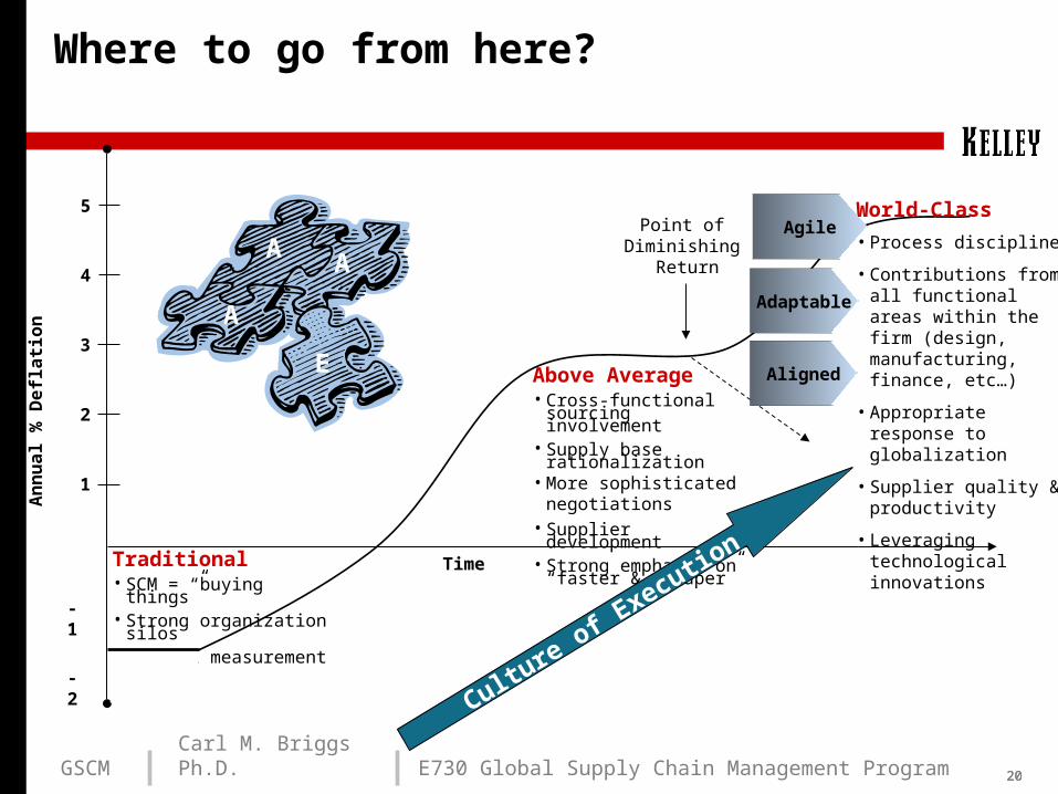
Where to go from here? A
nn
ua
l %
De
fla
tio
n
1
2
3
4
5
- 2
- 1
Time
Above Average• Cross-functional sourcing
involvement• Supply base
rationalization• More sophisticated
negotiations• Supplier development• Strong emphasis on
“faster & cheaper”Traditional• SCM = “buying things”• Strong organization silos• Minimal measurement
Point of Diminishing
Return
World-Class
• Process discipline
• Contributions from all functional areas within the firm (design, manufacturing, finance, etc…)
• Appropriate response to globalization
• Supplier quality & productivity
• Leveraging technological innovations
AA
A
E Aligned
Agile
Adaptable
Culture of E
xecution

21GSCM Carl M. Briggs Ph.D.
Exam review

222222GSCM Carl M. Briggs Ph.D. E730 Global Supply Chain Management Program
Possible exam questions…
Wednesday
• What decisions have to be made in setting up a SC network?
• What (types of) factors influence those decisions?
• Be able to discuss/evaluate the framework Chopra proposes for making facility location decisions.
• Be able to use a mile-centered or ton-centered gravity method for identifying optimal facility location.
Thursday
• Understand the use of DCF as a supply chain metric.
• Detail the steps in setting up and solving a facility location problem using Solver.
• Be able to set up and solve a decision tree as a tool for modeling uncertainty.
• Identify the key elements to successful supply chain turnaround (case).

232323

24GSCM Carl M. Briggs Ph.D.
Supplemental Slides

252525GSCM Carl M. Briggs Ph.D. E730 Global Supply Chain Management Program
Decision Tree Methodology:Trips Logistics
• Decide whether to lease warehouse space for the coming three years and the quantity to lease
• Long-term lease is currently cheaper than the spot market rate
• The manager anticipates uncertainty in demand and spot prices over the next three years
• Long-term lease is cheaper but could go unused if demand is lower than forecast; future spot market rates could also decrease
• Spot market rates are currently high, and the spot market would cost a lot if future demand is higher than expected

262626GSCM Carl M. Briggs Ph.D. E730 Global Supply Chain Management Program
Trips Logistics: Three Options
• Get all warehousing space from the spot market as needed
• Sign a three-year lease for a fixed amount of warehouse space and get additional requirements from the spot market
• Sign a flexible lease with a minimum change that allows variable usage of warehouse space up to a limit with additional requirement from the spot market
272727GSCM Carl M. Briggs Ph.D. E730 Global Supply Chain Management Program
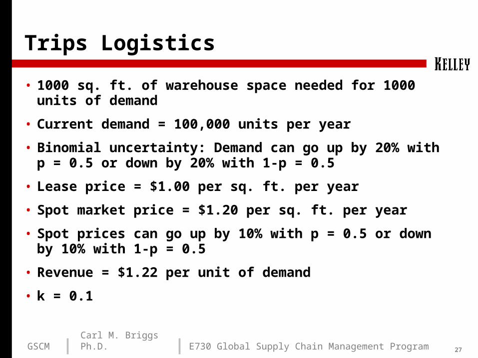
Trips Logistics
• 1000 sq. ft. of warehouse space needed for 1000 units of demand
• Current demand = 100,000 units per year
• Binomial uncertainty: Demand can go up by 20% with p = 0.5 or down by 20% with 1-p = 0.5
• Lease price = $1.00 per sq. ft. per year
• Spot market price = $1.20 per sq. ft. per year
• Spot prices can go up by 10% with p = 0.5 or down by 10% with 1-p = 0.5
• Revenue = $1.22 per unit of demand
• k = 0.1

282828GSCM Carl M. Briggs Ph.D. E730 Global Supply Chain Management Program
Trips Logistics Decision Tree (Fig. 6.2)
D=144
p=$1.45
D=144
p=$1.19
D=96
p=$1.45
D=144
p=$0.97
D=96
p=$1.19
D=96
p=$0.97
D=64
p=$1.45
D=64
p=$1.19
D=64
p=$0.97
D=120
p=$1.32
D=120
p=$1. 08
D=80
p=$1.32
D=80
p=$1.32
D=100
p=$1.20
0.25
0.25
0.25
0.25
0.250.25
0.25
0.25
Period 0
Period 1
Period 2
292929GSCM Carl M. Briggs Ph.D. E730 Global Supply Chain Management Program
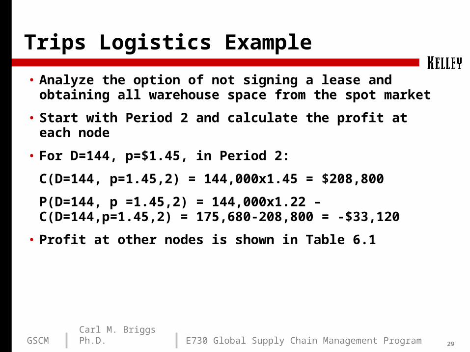
Trips Logistics Example
• Analyze the option of not signing a lease and obtaining all warehouse space from the spot market
• Start with Period 2 and calculate the profit at each node
• For D=144, p=$1.45, in Period 2:
C(D=144, p=1.45,2) = 144,000x1.45 = $208,800
P(D=144, p =1.45,2) = 144,000x1.22 – C(D=144,p=1.45,2) = 175,680-208,800 = -$33,120
• Profit at other nodes is shown in Table 6.1
303030GSCM Carl M. Briggs Ph.D. E730 Global Supply Chain Management Program
Trips Logistics Example
• Expected profit at each node in Period 1 is the profit during Period 1 plus the present value of the expected profit in Period 2
• Expected profit EP(D=, p=,1) at a node is the expected profit over all four nodes in Period 2 that may result from this node
• PVEP(D=,p=,1) is the present value of this expected profit and P(D=,p=,1), and the total expected profit, is the sum of the profit in Period 1 and the present value of the expected profit in Period 2

313131GSCM Carl M. Briggs Ph.D. E730 Global Supply Chain Management Program
Trips Logistics Example
• From node D=120, p=$1.32 in Period 1, there are four possible states in Period 2
• Evaluate the expected profit in Period 2 over all four states possible from node D=120, p=$1.32 in Period 1 to be
EP(D=120,p=1.32,1) = 0.25xP(D=144,p=1.45,2) +
0.25xP(D=144,p=1.19,2) +
0.25xP(D=96,p=1.45,2) +
0.25xP(D=96,p=1.19,2)
= 0.25x(-33,120)+0.25x4,320+0.25x(-22,080)+0.25x2,880
= -$12,000
323232GSCM Carl M. Briggs Ph.D. E730 Global Supply Chain Management Program
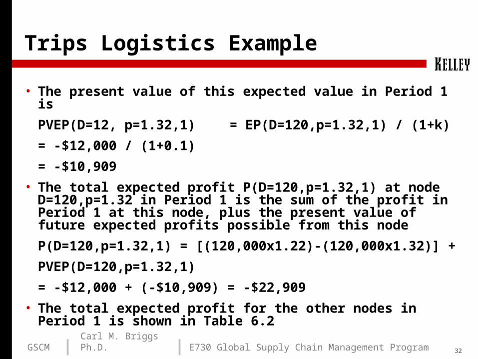
Trips Logistics Example
• The present value of this expected value in Period 1 is
PVEP(D=12, p=1.32,1) = EP(D=120,p=1.32,1) / (1+k)
= -$12,000 / (1+0.1)
= -$10,909
• The total expected profit P(D=120,p=1.32,1) at node D=120,p=1.32 in Period 1 is the sum of the profit in Period 1 at this node, plus the present value of future expected profits possible from this node
P(D=120,p=1.32,1) = [(120,000x1.22)-(120,000x1.32)] +
PVEP(D=120,p=1.32,1)
= -$12,000 + (-$10,909) = -$22,909
• The total expected profit for the other nodes in Period 1 is shown in Table 6.2
333333GSCM Carl M. Briggs Ph.D. E730 Global Supply Chain Management Program
Trips Logistics Example
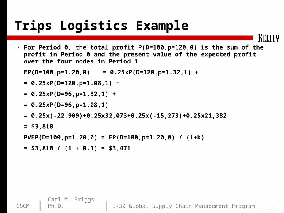
• For Period 0, the total profit P(D=100,p=120,0) is the sum of the profit in Period 0 and the present value of the expected profit over the four nodes in Period 1
EP(D=100,p=1.20,0) = 0.25xP(D=120,p=1.32,1) +
= 0.25xP(D=120,p=1.08,1) +
= 0.25xP(D=96,p=1.32,1) +
= 0.25xP(D=96,p=1.08,1)
= 0.25x(-22,909)+0.25x32,073+0.25x(-15,273)+0.25x21,382
= $3,818
PVEP(D=100,p=1.20,0) = EP(D=100,p=1.20,0) / (1+k)
= $3,818 / (1 + 0.1) = $3,471

343434GSCM Carl M. Briggs Ph.D. E730 Global Supply Chain Management Program
Trips Logistics Example
P(D=100,p=1.20,0) = 100,000x1.22-100,000x1.20 +
PVEP(D=100,p=1.20,0)
= $2,000 + $3,471 = $5,471
• Therefore, the expected NPV of not signing the lease and obtaining all warehouse space from the spot market is given by NPV(Spot Market) = $5,471
353535GSCM Carl M. Briggs Ph.D. E730 Global Supply Chain Management Program
Trips Logistics Example
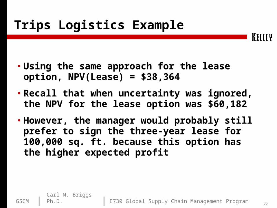
• Using the same approach for the lease option, NPV(Lease) = $38,364
• Recall that when uncertainty was ignored, the NPV for the lease option was $60,182
• However, the manager would probably still prefer to sign the three-year lease for 100,000 sq. ft. because this option has the higher expected profit
363636GSCM Carl M. Briggs Ph.D. E730 Global Supply Chain Management Program
Evaluating FlexibilityUsing Decision Trees
• Decision tree methodology can be used to evaluate flexibility within the supply chain
• Suppose the manager at Trips Logistics has been offered a contract where, for an upfront payment of $10,000, the company will have the flexibility of using between 60,000 sq. ft. and 100,000 sq. ft. of warehouse space at $1 per sq. ft. per year. Trips must pay $60,000 for the first 60,000 sq. ft. and can then use up to 40,000 sq. ft. on demand at $1 per sq. ft. as needed.
• Using the same approach as before, the expected profit of this option is $56,725
• The value of flexibility is the difference between the expected present value of the flexible option and the expected present value of the inflexible options
• The three options are listed in Table 6.7, where the flexible option has an expected present value $8,361 greater than the inflexible lease option (including the upfront $10,000 payment)
Top Related