


Languages
Pages
Legal


1
Deep Neural Networks for Acoustic Modeling
in Speech RecognitionGeoffrey Hinton, Li Deng, Dong Yu, George Dahl, Abdel-rahmanMohamed, Navdeep Jaitly, Andrew
Senior, Vincent Vanhoucke, Patrick Nguyen, Tara Sainath, andBrian Kingsbury
Abstract
Most current speech recognition systems use hidden Markov models (HMMs) to deal with the temporal variability
of speech and Gaussian mixture models to determine how well each state ofeach HMM fits a frame or a short window
of frames of coefficients that represents the acoustic input. An alternative way to evaluate the fit is to use a feed-
forward neural network that takes several frames of coefficients as input and produces posterior probabilities over
HMM states as output. Deep neural networks with many hidden layers, thatare trained using new methods have been
shown to outperform Gaussian mixture models on a variety of speech recognition benchmarks, sometimes by a large
margin. This paper provides an overview of this progress and represents the shared views of four research groups
who have had recent successes in using deep neural networks for acoustic modeling in speech recognition.
I. I NTRODUCTION
New machine learning algorithms can lead to significant advances in automatic speech recognition. The biggest
single advance occured nearly four decades ago with the introduction of the Expectation-Maximization (EM)
algorithm for training Hidden Markov Models (HMMs) (see [1], [2] for informative historical reviews of the
introduction of HMMs). With the EM algorithm, it became possible to develop speech recognition systems for
real world tasks using the richness of Gaussian mixture models (GMM) [3] to represent the relationship between
HMM states and the acoustic input. In these systems the acoustic input is typically represented by concatenating
Mel Frequency Cepstral Coefficients (MFCCs) or Perceptual Linear Predictive coefficients (PLPs) [4] computed
from the raw waveform, and their first- and second-order temporal differences [5]. This non-adaptive but highly-
engineered pre-processing of the waveform is designed to discard the large amount of information in waveforms that
is considered to be irrelevant for discrimination and to express the remaining information in a form that facilitates
discrimination with GMM-HMMs.
GMMs have a number of advantages that make them suitable for modeling the probability distributions over
vectors of input features that are associated with each state of an HMM. With enough components, they can model
Hinton, Dahl, Mohamed, and Jaitly are with the University of Toronto.
Deng and Yu are with Microsoft Research.
Senior, Vanhoucke and Nguyen are with Google Research.
Sainath and Kingsbury are with IBM Research.
April 27, 2012 DRAFT
2
probability distributions to any required level of accuracy and they are fairly easy to fit to data using the EM
algorithm. A huge amount of research has gone into ways of constraining GMMs to increase their evaluation speed
and to optimize the trade-off between their flexibility and the amount of training data available to avoid serious
overfitting [6].
The recognition accuracy of a GMM-HMM system can be further improved if it is discriminatively fine-tuned
after it has been generatively trained to maximize its probability of generating the observed data, especially if
the discriminative objective function used for training isclosely related to the error rate on phones, words or
sentences[7]. The accuracy can also be improved by augmenting (or concatenating) the input features (e.g., MFCCs)
with “tandem” or bottleneck features generated using neural networks [8], [9]. GMMs are so successful that it is
difficult for any new method to outperform them for acoustic modeling.
Despite all their advantages, GMMs have a serious shortcoming – they are statistically inefficient for modeling
data that lie on or near a non-linear manifold in the data space. For example, modeling the set of points that lie very
close to the surface of a sphere only requires a few parameters using an appropriate model class, but it requires a
very large number of diagonal Gaussians or a fairly large number of full-covariance Gaussians. Speech is produced
by modulating a relatively small number of parameters of a dynamical system [10], [11] and this implies that its true
underlying structure is much lower-dimensional than is immediately apparent in a window that contains hundreds
of coefficients. We believe, therefore, that other types of model may work better than GMMs for acoustic modeling
if they can more effectively exploit information embedded in a large window of frames.
Artificial neural networks trained by backpropagating error derivatives have the potential to learn much better
models of data that lie on or near a non-linear manifold. In fact two decades ago, researchers achieved some success
using artificial neural networks with a single layer of non-linear hidden units to predict HMM states from windows
of acoustic coefficients [9]. At that time, however, neitherthe hardware nor the learning algorithms were adequate
for training neural networks with many hidden layers on large amounts of data and the performance benefits of
using neural networks with a single hidden layer were not sufficiently large to seriously challenge GMMs. As a
result, the main practical contribution of neural networksat that time was to provide extra features in tandem or
bottleneck systems.
Over the last few years, advances in both machine learning algorithms and computer hardware have led to more
efficient methods for training deep neural networks (DNNs) that contain many layers of non-linear hidden units and
a very large output layer. The large output layer is requiredto accommodate the large number of HMM states that
arise when each phone is modelled by a number of different “triphone” HMMs that take into account the phones on
either side. Even when many of the states of these triphone HMMs are tied together, there can be thousands of tied
states. Using the new learning methods, several different research groups have shown that DNNs can outperform
GMMs at acoustic modeling for speech recognition on a variety of datasets including large datasets with large
vocabularies.
This review paper aims to represent the shared views of research groups at the University of Toronto, Microsoft
Research (MSR), Google and IBM Research, who have all had recent successes in using DNNs for acoustic
April 27, 2012 DRAFT

3
modeling. The paper starts by describing the two-stage training procedure that is used for fitting the DNNs. In the
first stage, layers of feature detectors are initialized, one layer at a time, by fitting a stack of generative models,
each of which has one layer of latent variables. These generative models are trained without using any information
about the HMM states that the acoustic model will need to discriminate. In the second stage, each generative model
in the stack is used to initialize one layer of hidden units ina DNN and the whole network is then discriminatively
fine-tuned to predict the target HMM states. These targets are obtained by using a baseline GMM-HMM system to
produce a forced alignment.
In this paper we review exploratory experiments on the TIMITdatabase [12], [13] that were used to demonstrate
the power of this two-stage training procedure for acousticmodeling. The DNNs that worked well on TIMIT were
then applied to five different large vocabulary, continuousspeech recognition tasks by three different research groups
whose results we also summarize. The DNNs worked well on all of these tasks when compared with highly-tuned
GMM-HMM systems and on some of the tasks they outperformed the state-of-the-art by a large margin. We also
describe some other uses of DNNs for acoustic modeling and some variations on the training procedure.
II. T RAINING DEEP NEURAL NETWORKS
A deep neural network (DNN) is a feed-forward, artificial neural network that has more than one layer of hidden
units between its inputs and its outputs. Each hidden unit,j, typically uses the logistic function1 to map its total
input from the layer below,xj , to the scalar state,yj that it sends to the layer above.
yj = logistic(xj) =1
1 + e−xj, xj = bj +
∑
i
yiwij , (1)
wherebj is the bias of unitj, i is an index over units in the layer below, andwij is a the weight on a connection
to unit j from unit i in the layer below. For multiclass classification, output unit j converts its total input,xj , into
a class probability,pj , by using the “softmax” non-linearity:
pj =exp(xj)
∑
k exp(xk), (2)
wherek is an index over all classes.
DNN’s can be discriminatively trained by backpropagating derivatives of a cost function that measures the
discrepancy between the target outputs and the actual outputs produced for each training case[14]. When using the
softmax output function, the natural cost functionC is the cross-entropy between the target probabilitiesd and the
outputs of the softmax,p:
C = −∑
j
dj log pj , (3)
where the target probabilities, typically taking values ofone or zero, are the supervised information provided to
train the DNN classifier.
1The closely related hyberbolic tangent is also often used and any function with a well-behaved derivative can be used.
April 27, 2012 DRAFT

4
For large training sets, it is typically more efficient to compute the derivatives on a small, random “mini-batch”
of training cases, rather than the whole training set, before updating the weights in proportion to the gradient. This
stochastic gradient descent method can be further improvedby using a “momentum” coefficient,0 < α < 1, that
smooths the gradient computed for mini-batcht, thereby damping oscillations across ravines and speedingprogress
down ravines:
∆wij(t) = α∆wij(t − 1) − ǫ∂C
∂wij(t). (4)
The update rule for biases can be derived by treating them as weights on connections coming from units that always
have a state of1.
To reduce overfitting, large weights can be penalized in proportion to their squared magnitude, or the learning
can simply be terminated at the point at which performance ona held-out validation set starts getting worse[9]. In
DNNs with full connectivity between adjacent layers, the initial weights are given small random values to prevent
all of the hidden units in a layer from getting exactly the same gradient.
DNN’s with many hidden layers are hard to optimize. Gradientdescent from a random starting point near the
origin is not the best way to find a good set of weights and unless the initial scales of the weights are carefully
chosen [15], the backpropagated gradients will have very different magnitudes in different layers. In addition to
the optimization issues, DNNs may generalize poorly to held-out test data. DNNs with many hidden layers and
many units per layer are very flexible models with a very largenumber of parameters. This makes them capable of
modeling very complex and highly non-linear relationshipsbetween inputs and outputs. This ability is important
for high-quality acoustic modeling, but it also allows themto model spurious regularities that are an accidental
property of the particular examples in the training set, which can lead to severe overfitting. Weight penalties or
early-stopping can reduce the overfitting but only by removing much of the modeling power. Very large training sets
[16] can reduce overfitting whilst preserving modeling power, but only by making training very computationally
expensive. What we need is a better method of using the information in the training set to build multiple layers of
non-linear feature detectors.
A. Generative pre-training
Instead of designing feature detectors to be good for discriminating between classes, we can start by designing
them to be good at modeling the structure in the input data. The idea is to learn one layer of feature detectors at
a time with the states of the feature detectors in one layer acting as the data for training the next layer. After this
generative “pre-training”, the multiple layers of featuredetectors can be used as a much better starting point for
a discriminative “fine-tuning” phase during which backpropagation through the DNN slightly adjusts the weights
found in pre-training [17]. Some of the high-level featurescreated by the generative pre-training will be of little
use for discrimination, but others will be far more useful than the raw inputs. The generative pre-training finds a
region of the weight-space that allows the discriminative fine-tuning to make rapid progress, and it also significantly
reduces overfitting [18].
April 27, 2012 DRAFT

5
A single layer of feature detectors can be learned by fitting agenerative model with one layer of latent variables
to the input data. There are two broad classes of generative model to choose from. Adirectedmodel generates
data by first choosing the states of the latent variables froma prior distribution and then choosing the states of the
observable variables from their conditional distributions given the latent states. Examples of directed models with
one layer of latent variables are factor analysis, in which the latent variables are drawn from an isotropic Gaussian,
and GMMs, in which they are drawn from a discrete distribution. An undirectedmodel has a very different way of
generating data. Instead of using one set of parameters to define a prior distribution over the latent variables and a
separate set of parameters to define the conditional distributions of the observable variables given the values of the
latent variables, an undirected model uses a single set of parameters,W, to define the joint probability of a vector
of values of the observable variables,v, and a vector of values of the latent variables,h, via an energy function,
E:
p(v,h;W) =1
Ze−E(v,h;W), Z =
∑
v′,h′
e−E(v′,h′;W), (5)
whereZ is called the “partition function”.
If many different latent variables interact non-linearly to generate each data vector, it is difficult to infer the states
of the latent variables from the observed data in a directed model because of a phenomenon known as “explaining
away” [19]. In undirected models, however, inference is easy provided the latent variables do not have edges linking
them. Such a restricted class of undirected models is ideal for layerwise pre-training because each layer will have
an easy inference procedure.
We start by describing an approximate learning algorithm for a restricted Boltzmann machine (RBM) which
consists of a layer of stochastic binary “visible” units that represent binary input data connected to a layer of
stochastic binary hidden units that learn to model significant non-independencies between the visible units [20]. There
are undirected connections between visible and hidden units but no visible-visible or hidden-hidden connections.
An RBM is a type of Markov Random Field (MRF) but differs from most MRF’s in several ways: It has a bipartite
connectivity graph; it does not usually share weights between different units; and a subset of the variables are
unobserved, even during training.
B. An efficient learning procedure for RBMs
A joint configuration, (v,h) of the visible and hidden units of an RBM has an energy given by:
E(v,h) = −∑
i∈visible
aivi −∑
j∈hidden
bjhj −∑
i,j
vihjwij (6)
wherevi, hj are the binary states of visible uniti and hidden unitj, ai, bj are their biases andwij is the weight
between them. The network assigns a probability to every possible pair of a visible and a hidden vector via this
energy function as in Eqn. (5) and the probability that the network assigns to a visible vector,v, is given by
summing over all possible hidden vectors:
p(v) =1
Z
∑
h
e−E(v,h) (7)
April 27, 2012 DRAFT

6
The derivative of the log probability of a training set with respect to a weight is surprisingly simple:
1
N
n=N∑
n=1
∂ log p(vn)
∂wij
=<vihj>data − <vihj>model (8)
whereN is the size of the training set and the angle brackets are usedto denote expectations under the distribution
specified by the subscript that follows. The simple derivative in Eqn.(8) leads to a very simple learning rule for
performing stochastic steepest ascent in the log probability of the training data:
∆wij = ǫ(<vihj>data − <vihj>model) (9)
whereǫ is a learning rate.
The absence of direct connections between hidden units in anRBM makes it is very easy to get an unbiased
sample of<vihj>data. Given a randomly selected training case,v, the binary state,hj , of each hidden unit,j, is
set to1 with probability
p(hj = 1 | v) = logistic(bj +∑
i
viwij) (10)
and vihj is then an unbiased sample. The absence of direct connections between visible units in an RBM makes
it very easy to get an unbiased sample of the state of a visibleunit, given a hidden vector
p(vi = 1 | h) = logistic(ai +∑
j
hjwij). (11)
Getting an unbiased sample of<vihj >model, however, is much more difficult. It can be done by starting at
any random state of the visible units and performing alternating Gibbs sampling for a very long time. Alternating
Gibbs sampling consists of updating all of the hidden units in parallel using Eqn.(10) followed by updating all of
the visible units in parallel using Eqn.(11).
A much faster learning procedure called “contrastive divergence” (CD) was proposed in [20]. This starts by
setting the states of the visible units to a training vector.Then the binary states of the hidden units are all computed
in parallel using Eqn.(10). Once binary states have been chosen for the hidden units, a “reconstruction” is produced
by setting eachvi to 1 with a probability given by Eqn.(11). Finally, the states ofthe hidden units are updated
again. The change in a weight is then given by
∆wij = ǫ(<vihj>data − <vihj>recon) (12)
A simplified version of the same learning rule that uses the states of individual units instead of pairwise products
is used for the biases.
Contrastive divergence works well even though it is only crudely approximating the gradient of the log probability
of the training data [20]. RBMs learn better generative models if more steps of alternating Gibbs sampling are used
before collecting the statistics for the second term in the learning rule, but for the purposes of pre-training feature
detectors, more alternations are generally of little valueand all the results reviewed here were obtained using
CD1 which does a single full step of alternating Gibbs sampling after the initial update of the hidden units. To
suppress noise in the learning, the real-valued probabilities rather than binary samples are generally used for the
April 27, 2012 DRAFT

7
reconstructions and the subsequent states of the hidden units, but it is important to use sampled binary values for the
first computation of the hidden states because the sampling noise acts as a very effective regularizer that prevents
overfitting [21].
C. Modeling real-valued data
Real-valued data, such as MFCCs, are more naturally modeledby linear variables with Gaussian noise and the
RBM energy function can be modified to accommodate such variables, giving a Gaussian-Bernoulli RBM (GRBM):
E(v,h) =∑
i∈vis
(vi − ai)2
2σ2i
−∑
j∈hid
bjhj −∑
i,j
vi
σi
hjwij (13)
whereσi is the standard deviation of the Gaussian noise for visible unit i.
The two conditional distributions required for CD1 learning are:
p(hj |v) = logistic
(
bj +∑
i
vi
σi
wij
)
(14)
p(vi|h) = N
ai + σi
∑
j
hjwij , σ2i
(15)
whereN (µ, σ2) is a Gaussian. Learning the standard deviations of a GRBM is problematic for reasons described
in [21], so for pre-training using CD1, the data are normalized so that each coefficient has zero mean and unit
variance, the standard deviations are set to1 when computingp(v|h), and no noise is added to the reconstructions.
This avoids the issue of deciding the right noise level.
D. Stacking RBMs to make a deep belief network
After training an RBM on the data, the inferred states of the hidden units can be used as data for training
another RBM that learns to model the significant dependencies between the hidden units of the first RBM. This
can be repeated as many times as desired to produce many layers of non-linear feature detectors that represent
progressively more complex statistical structure in the data. The RBMs in a stack can be combined in a surprising
way to produce a single, multi-layer generative model called a deep belief net (DBN) [22]. Even though each RBM
is an undirected model, the DBN2 formed by the whole stack is a hybrid generative model whose top two layers
are undirected (they are the final RBM in the stack) but whose lower layers have top-down, directed connections
(see figure 1).
To understand how RBMs are composed into a DBN it is helpful torewrite Eqn.(7) and to make explicit the
dependence onW:
p(v;W) =∑
h
p(h;W)p(v|h;W), (16)
2Not to be confused with a Dynamic Bayesian Net which is a type ofdirected model of temporal data that unfortunately has the same
acronym.
April 27, 2012 DRAFT

8
GRBM
RBM
RBM DBN
DBN-DNN
copy
copy
softmax
1W
2W
3W
3W
2W
1W
TW3
TW2
TW1
04
W
Fig. 1. The sequence of operations used to create a DBN with three hidden layers and to convert it to a pre-trained DBN-DNN.First a
GRBM is trained to model a window of frames of real-valued acoustic coefficients. Then the states of the binary hidden units of the GRBM
are used as data for training an RBM. This is repeated to create as many hidden layers as desired. Then the stack of RBMs is converted
to a single generative model, a DBN, by replacing the undirected connections of the lower level RBMs by top-down, directedconnections.
Finally, a pre-trained DBN-DNN is created by adding a “softmax” output layer that contains one unit for each possible state of each HMM.
The DBN-DNN is then discriminatively trained to predict the HMM state corresponding to the central frame of the input window in a forced
alignment.
where p(h;W) is defined as in Eqn.(7) but with the roles of the visible and hidden units reversed. Now it is
clear that the model can be improved by holdingp(v|h;W) fixed after training the RBM, but replacing the prior
over hidden vectorsp(h;W) by a better prior,i.e. a prior that is closer to the aggregated posterior over hidden
vectors that can be sampled by first picking a training case and then inferring a hidden vector using Eqn.(14). This
aggregated posterior is exactly what the next RBM in the stack is trained to model.
As shown in [22], there is a series of variational bounds on the log probability of the training data, and furthermore,
each time a new RBM is added to the stack, the variational bound on the new and deeper DBN is better than the
previous variational bound, provided the new RBM is initialized and learned in the right way. While the existence
of a bound that keeps improving is mathematically reassuring, it does not answer the practical issue, addressed in
this review paper, of whether the learned feature detectorsare useful for discrimination on a task that is unknown
while training the DBN. Nor does it guarantee that anything improves when we use efficient short-cuts such as
CD1 training of the RBMs.
April 27, 2012 DRAFT

9
One very nice property of a DBN that distinguishes it from other multilayer, directed, non-linear generative
models, is that it is possible to infer the states of the layers of hidden units in a single forward pass. This inference,
which is used in deriving the variational bound, is not exactly correct but it is fairly accurate. So after learning a
DBN by training a stack of RBMs, we can jettison the whole probabilistic framework and simply use the generative
weights in the reverse direction as a way of initializing allthe feature detecting layers of a deterministic feed-forward
DNN. We then just add a final softmax layer and train the whole DNN discriminatively3.
E. Interfacing a DNN with an HMM
After it has been discriminatively fine-tuned, a DNN outputsprobabilities of the form
p(HMMstate|AcousticInput). But to compute a Viterbi alignment or to run the forward-backward algorithm
within the HMM framework we require the likelihoodp(AcousticInput|HMMstate). The posterior probabilities
that the DNN outputs can be converted into the scaled likelihood by dividing them by the frequencies of the
HMM-states in the forced alignment that is used for fine-tuning the DNN [9]. All of the likelihoods produced in
this way are scaled by the same unknown factor ofp(AcousticInput), but this has no effect on the alignment.
Although this conversion appears to have little effect on some recognition tasks, it can be important for tasks
where training labels are highly unbalanced (e.g., with many frames of silences).
III. PHONETIC CLASSIFICATION AND RECOGNITION ONTIMIT
The TIMIT dataset provides a simple and convenient way of testing new approaches to speech recognition.
The training set is small enough to make it feasible to try many variations of a new method and many existing
techniques have already been benchmarked on the core test set so it is easy to see if a new approach is promising
by comparing it with existing techniques that have been implemented by their proponents [23]. Experience has
shown that performance improvements on TIMIT do not necessarily translate into performance improvements on
large vocabulary tasks with less controlled recording conditions and much more training data. Nevertheless, TIMIT
provides a good starting point for developing a new approach, especially one that requires a challenging amount of
computation.
Mohamedet. al. [12] showed that a DBN-DNN acoustic model outperformed the best published recognition
results on TIMIT at about the same time as Sainathet. al. [23] achieved a similar improvement on TIMIT by
applying state-of-the-art techniques developed for largevocabulary recognition. Subsequent work combined the
two approaches by using state-of-the-art, discriminatively trained (DT) speaker-dependent features as input to the
DBN-DNN [24], but this produced little further improvement, probably because the hidden layers of the DBN-DNN
were already doing quite a good job of progressively eliminating speaker differences [25].
The DBN-DNNs that worked best on the TIMIT data formed the starting point for subsequent experiments
on much more challenging, large vocabulary tasks that were too computationally intensive to allow extensive
3Unfortunately, a DNN that is pre-trained generatively as a DBN is often still called a DBN in the literature. For clarity we call it a DBN-DNN.
April 27, 2012 DRAFT

10
TABLE I
Comparisons among the reported speaker-independent phonetic recognition accuracy results on TIMIT core test set with192 sentences
Method PER
CD-HMM [26] 27.3%
Augmented conditional Random Fields [26] 26.6%
Randomly initialized recurrent Neural Nets [27] 26.1%
Bayesian Triphone GMM-HMM [28] 25.6%
Monophone HTMs [29] 24.8%
Heterogeneous Classifiers [30] 24.4%
Monophone randomly initialized DNNs (6 layers)[13] 23.4%
Monophone DBN-DNNs (6 layers) [13] 22.4%
Monophone DBN-DNNs with MMI training [31] 22.1%
Triphone GMM-HMMs discriminatively trained w/ BMMI [32] 21.7%
Monophone DBN-DNNs on fbank (8 layers) [13] 20.7%
Monophone mcRBM-DBN-DNNs on fbank (5 layers) [33] 20.5%
Monophone convolutional DNNs on fbank (3 layers) [34] 20.0%
exploration of variations in the architecture of the neuralnetwork, the representation of the acoustic input or the
training procedure.
For simplicity, all hidden layers always had the same size, but even with this constraint it was impossible to
train all possible combinations of number of hidden layers [1, 2, 3, 4, 5, 6, 7, 8], number of units per layer [512,
1024, 2048, 3072] and number of frames of acoustic data in the input layer [7,11, 15, 17, 27, 37]. Fortunately,
the performance of the networks on the TIMIT core test set wasfairly insensitive to the precise details of the
architecture and the results in [13] suggest that any combination of the numbers in boldface probably has an error
rate within about2% of the very best combination. This robustness is crucial formethods such as DBN-DNNs
that have a lot of tuneable meta-parameters. Our consistentfinding is that multiple hidden layers always worked
better than one hidden layer and, with multiple hidden layers, pre-training always improved the results on both the
development and test sets in the TIMIT task. Details of the learning rates, stopping criteria, momentum, L2 weight
penalties and mini-batch size for both the pre-training andfine-tuning are given in [13].
Table I compares DBN-DNNs with a variety of other methods on the TIMIT core test set. For each type of
DBN-DNN the architecture that performed best on the development set is reported. All methods use MFCCs as
inputs except for the three marked “fbank” that use log Mel-scale filter-bank outputs.
A. Pre-processing the waveform for deep neural networks
State-of-the-art ASR systems do not use filter-bank coefficients as the input representation because they are
strongly correlated so modeling them well requires either full covariance Gaussians or a huge number of diagonal
Gaussians. MFCCs offer a more suitable alternative as theirindividual components are roughly independent so they
are much easier to model using a mixture of diagonal covariance Gaussians. DBN-DNNs do not require uncorrelated
April 27, 2012 DRAFT

11
data and, on the TIMIT database, the work reported in [13] showed that the best performing DBN-DNNs trained
with filter-bank features had a phone error rate 1.7% lower than the best performing DBN-DNNs trained with
MFCCs (see Table I).
B. Fine-tuning DBN-DNNs to optimize mutual information
In the experiments using TIMIT discussed above, the DNNs were fine-tuned to optimize the per frame cross-
entropy between the target HMM state and the predictions. The transition parameters and language model scores
were obtained from an HMM-like approach and were trained independently of the DNN weights. However, it has
long been known that sequence classification criteria, which are more directly correlated with the overall word or
phone error rate, can be very helpful in improving recognition accuracy [7], [35] and the benefit of using such
sequence classification criteria with shallow neural networks has already been shown by [36], [37], [38]. In the more
recent work reported in [31], one popular type of sequence classification criterion, maximum mutual information
or MMI, proposed as early as 1986 [7], was successfully applied to learn DBN-DNN weights for the TIMIT phone
recognition task. MMI optimizes the conditional probability p(l1:T |v1:T ) of the whole sequence of labels,l1:T , with
length T, given the whole visible feature utterancev1:T , or equivalently the hidden feature sequenceh1:T extracted
by the DNN:
p(l1:T |v1:T ) = p(l1:T |h1:T ) =exp(
∑Tt=1 γijφij(lt−1, lt) +
∑Tt=1
∑Dd=1 λlt,dhtd)
Z(h1:T ), (17)
where the transition featureφij(lt−1, lt) takes on a value of one iflt−1 = i and lt = j, and otherwise takes on
a value of zero, whereγij is the parameter associated with this transition feature,htd is the d-th dimension of
the hidden unit value at thet-th frame at the final layer of the DNN, and whereD is the number of units in the
final hidden layer. Note the objective function of Eqn.(17) derived from mutual information [35] is the same as
the conditional likelihood associated with a specialized linear-chain conditional random field. Here, it is the top
most layer of the DNN below the softmax layer, not the raw speech coefficients of MFCC or PLP, that provides
“features” to the conditional random field.
To optimize the log conditional probabilityp(ln1:T |vn1:T ) of the n-th utterance, we take the gradient over the
activation parametersλkd, transition parametersγij , and the lower-layer weights of the DNN,wij , according to
∂ log p(ln1:T |vn1:T )
∂λkd
=T∑
t=1
(δ(lnt = k) − p(lnt = k|vn1:T ))hn
td (18)
∂ log p(ln1:T |vn1:T )
∂γij
=
T∑
t=1
[δ(lnt−1 = i, lnt = j) − p(lnt−1 = i, lnt = j|vn1:T )] (19)
∂ log p(ln1:T |vn1:T )
∂wij
=
T∑
t=1
[λltd−
K∑
k=1
p(lnt = k|vn1:T )λkd] × hn
td(1 − hntd)x
nti (20)
Note that the gradient∂ log p(ln1:T |vn
1:T )∂wij
above can be viewed as back-propagating the errorδ(lnt = k) − p(lnt =
k|vn1:T ), vs. δ(lnt = k) − p(lnt = k|vn
t ) in the frame-based training algorithm.
April 27, 2012 DRAFT

12
In implementing the above learning algorithm for a DBN-DNN,the DNN weights can first be fine-tuned to
optimize the per frame cross entropy. The transition parameters can be initialized from the combination of the
HMM transition matrices and the “phone language” model scores, and can be further optimized by tuning the
transition features while fixing the DNN weights before the joint optimization. Using the joint optimization with
careful scheduling, we observe that the sequential MMI training can outperform the frame-level training by about
5% relative within the same system in the same laboratory.
C. Convolutional DNNs for phone classification and recognition
All the previously cited work reported phonerecognition results on the TIMIT database. In recognition
experiments, the input is the acoustic input for the whole utterance while the output is the spoken phonetic sequence.
A decoding process using a phone language model is used to produce this output sequence. Phoneticclassification
is a different task where the acoustic input has already beenlabeled with the correct boundaries between different
phonetic units and the goal is to classify these phones conditioned on the given boundaries. In [39] convolutional
DBN-DNNs were introduced and successfully applied to various audio tasks including phone classification on the
TIMIT database. In this model, the RBM was made convolutional in time by sharing weights between hidden
units that detect the same feature at different times. A max-pooling operation was then performed which takes the
maximal activation over a pool of adjacent hidden units thatshare the same weights but apply them at different
times. This yields some temporal invariance.
Although convolutional models along the temporal dimension achieved good classification results [39], applying
them to phone recognition is not straightforward. This is because temporal variations in speech can be partially
handled by the dynamic programing procedure in the HMM component and those aspects of temporal variation that
cannot be adequately handled by the HMM can be addressed moreexplicitly and effectively by hidden trajectory
models [40].
The work reported in [34] applied local convolutional filters with max-pooling to thefrequencyrather than
time dimension of the spectrogram. Sharing-weights and poolingover frequency was motivated by the shifts in
formant frequencies caused by speaker variations. It provides some speaker invariance while also offering noise
robustness due to the band-limited nature of the filters. [34] only used weight-sharing and max-pooling across
nearby frequencies because, unlike features that occur at different positions in images, acoustic features occuring
at very different frequencies are very different.
D. A summary of the differences between DNNs and GMMs
Here we summarize the main differences between the DNNs and GMMs used in the TIMIT experiments described
so far in this paper. First, one major element of the DBN-DNN,the RBM which serves as the building block for
pre-training, is an instance of “product of experts” [20], in contrast to mixture models that are a “sum of experts”.
4. Mixture models with a large number of components use their parameters inefficiently because each parameter
4Product models have only very recently been explored in speech processing; e.g., [41].
April 27, 2012 DRAFT

13
only applies to a very small fraction of the data whereas eachparameter of a product model is constrained by a
large fraction of the data. Second, while both DNNs and GMMs are nonlinear models, the nature of the nonlinearity
is very different. Third, DNNs are good at exploiting multiple frames of input coefficients whereas GMMs that
use diagonal covariance matrices benefit much less from multiple frames because they require decorrelated inputs.
Finally, DNNs are learned using stochastic gradient descent, while GMMs are learned using the EM algorithm or
its extensions [35] which makes GMM learning much easier to parallelize on a cluster machine.
IV. COMPARING DBN-DNNS WITH GMMS FORLARGE-VOCABULARY SPEECHRECOGNITION
The success of DBN-DNNs on TIMIT tasks starting in 2009 motivated more ambitious experiments with much
larger vocabularies and more varied speaking styles. In this section, we review experiments by three different speech
groups on five different benchmark tasks for large vocabulary speech recognition. To make DBN-DNNs work really
well on large vocabulary tasks it is important to replace themonophone HMMs used for TIMIT (and also for
early neural network/HMM hybrid systems) with triphone HMMs that have many thousands of tied states [42].
Predicting these context-dependent states provides several advantages over monophone targets. They supply more
bits of information per frame in the labels. They also make itpossible to use a more powerful triphone HMM
decoder and to exploit the sensible classes discovered by the decision tree clustering that is used to tie the states of
different triphone HMMs. Using context-dependent HMM states, it is possible to outperform state-of-the-art BMMI
trained GMM-HMM systems with a two-hidden-layer neural network without using any pre-training [43], though
using more hidden layers and pre-training works even better.
A. Bing-Voice-Search speech recognition task
The first successful use of acoustic models based on DBN-DNNsfor a large vocabulary task used data collected
from the Bing mobile voice search application (BMVS). The task used 24 hours of training data with a high degree
of acoustic variability caused by noise, music, side-speech, accents, sloppy pronunciation, hesitation, repetition,
interruptions, and mobile phone differences. The results reported in [42] demonstrated that the best DNN-HMM
acoustic model trained with context-dependent states as targets achieved a sentence accuracy of 69.6% on the test
set, compared with 63.8% for a strong, MPE trained GMM-HMM baseline.
The DBN-DNN used in the experiments was based on one of the DBN-DNNs that worked well for the TIMIT
task. It used five pre-trained layers of hidden units with 2,048 units per layer and was trained to classify the central
frame of an 11 frame acoustic context window using 761 possible context-dependent states as targets. In addition
to demonstrating that a DBN-DNN could provide gains on a large vocabulary task, several other important issues
were explicitly investigated in [42]. It was found that using tied triphone context-dependent state targets was crucial
and clearly superior to using monophone state targets, evenwhen the latter were derived from the same forced
alignment with the same baseline. It was also confirmed that the lower the error rate of the system used during forced
alignment to generate frame level training labels for the neural net, the lower the error rate of the final neural-net
based system. This effect was consistent across all the alignments they tried, including monophone alignments,
April 27, 2012 DRAFT
14
alignments from maximum likelihood trained GMM-HMM systems, and alignments from discriminatively trained
GMM-HMM systems.
Further work after that of [42] extended the DNN-HMM acoustic model from 24 hours of training data to 48
hours, and explored the respective roles of pre-training and fine-tuning the DBN-DNN [44]. As expected, pre-training
is helpful in training the DBN-DNN because it initializes the DBN-DNN weights to a point in the weight-space
from which fine-tuning is highly effective. However, a moderate increase of the amount of unlabeled pre-training
data has an insignificant effect on the final recognition results (69.6% to 69.8%), as long as the original training set
is fairly large. By contrast, the same amount of additional labeled fine-tuning training data significantly improves
the performance of the DNN-HMMs (accuracy from 69.6% to 71.7%).
B. Switchboard speech recognition task
The DNN-HMM training recipe developed for the Bing voice search data was applied unaltered to the Switchboard
speech recognition task [43] to confirm the suitability of DNN-HMM acoustic models for large vocabulary tasks.
Before this work, DNN-HMM acoustic models had only been trained with up to 48 hours of data [44] and hundreds
of tied triphone states as targets, whereas this work used over 300 hours of training data and thousands of tied
triphone states as targets. Furthermore, Switchboard is a publicly available speech-to-text transcription benchmark
task that allows much more rigorous comparisons among techniques.
The baseline GMM-HMM system on the Switchboard task was trained using the standard 309-hour Switchboard-I
training set. 13-dimensional PLP features with windowed mean-variance normalization were concatenated with up
to third-order derivatives and reduced to 39 dimensions by HDLA, a form of linear discriminant analysis (LDA).
The speaker-independent crossword triphones used the common left-to-right 3-state topology and shared 9304 tied
states.
The baseline GMM-HMM system had a mixture of 40 Gaussians per(tied) HMM state that were first trained
generatively to optimize a maximum likelihood (ML) criterion and then refined discriminatively to optimize a
boosted maximum-mutual-information (BMMI) criterion. A seven-hidden-layer DBN-DNN with 2048 units in each
layer and full connectivity between adjacent layers replaced the GMM in the acoustic model. The trigram language
model, used for both systems, was trained on the training transcripts of the 2000-hours of the Fisher corpus and
interpolated with a trigram model trained on written text.
The primary test set is the FSH portion of the 6.3-hour Spring2003 NIST rich transcription set (RT03S). Table
II extracted from the literature shows a summary of the core results. Using a DNN reduced the word-error rate
(WER) from the 27.4% of the baseline GMM-HMM (trained with BMMI) to 18.5% – a 33% relative reduction.
The DNN-HMM system trained on 309 hours performs as well as combining several speaker-adaptive, multi-pass
systems which use Vocal Tract Length Normalization (VTLN) and nearly seven times as much acoustic training
data (the 2000h Fisher corpus) (18.6%, last row).
Detailed experiments [43] on the Switchboard task confirmedthat the remarkable accuracy gains from the DNN-
HMM acoustic model are due to the direct modeling of tied triphone states using the DBN-DNN, the effective
April 27, 2012 DRAFT

15
TABLE II
Comparing five different DBN-DNN acoustic models with two strong GMM-HMM baseline systems that are discriminatively trained (DT).
Speaker-independent (SI) training on 309 hours of data and single-pass decoding were used for all models except for the GMM-HMM system
shown on the last row which used speaker adaptive (SA) training with 2000 hours of data and multi-pass decoding includinghypotheses
combination. In the table, “40 mix” means a mixture of 40 Gaussians per HMM state and “15.2 nz” means 15.2 million, non-zero weights.
Word-error rates (WER) in % are shown for two separate test sets, Hub500-SWB and RT03S-FSH.
modeling #params WER
technique [106] Hub5’00-SWBRT03S-FSH
GMM, 40 mix DT 309h SI 29.4 23.6 27.4
NN 1 hidden-layer×4634 units 43.6 26.0 29.4
+ 2×5 neighboring frames 45.1 22.4 25.7
DBN-DNN 7 hidden layers×2048 units 45.1 17.1 19.6
+ updated state alignment 45.1 16.4 18.6
+ sparsification 15.2 nz 16.1 18.5
GMM 72 mix DT 2000h SA 102.4 17.1 18.6
exploitation of neighboring frames by the DBN-DNN, and the strong modeling power of deeper networks, as was
discovered in the Bing voice search task [44], [42]. Pre-training the DBN-DNN leads to the best results but it is
not critical: For this task, it provides an absolute WER reduction of less than 1% and this gain is even smaller
when using five or more hidden layers. For under-resourced languages that have smaller amounts of labeled data,
pre-training is likely to be far more helpful.
Further study [45] suggests that feature-engineering techniques such as HLDA and VTLN, commonly used in
GMM-HMMs, are more helpful for shallow neural nets than for DBN-DNNs, presumably because DBN-DNNs are
able to learn appropriate features in their lower layers.
C. Google Voice Input speech recognition task
Google Voice Input transcribes voice search queries, shortmessages, emails and user actions from mobile devices.
This is a large vocabulary task that uses a language model designed for a mixture of search queries and dictation.
Google’s full-blown model for this task, which was built from a very large corpus, uses a speaker-independent
GMM-HMM model composed of context dependent cross-word triphone HMMs that have a left-to-right, three-
state topology. This model has a total of 7969 senone states and uses as acoustic input PLP features that have been
transformed by LDA. Semi-Tied Covariances (STC) are used inthe GMMs to model the LDA transformed features
and BMMI[46] was used to train the model discriminatively.
Jaitly et. al. [47] used this model to obtain approximately 5,870 hours of aligned training data for a DBN-DNN
acoustic model that predicts the 7,969 HMM state posteriorsfrom the acoustic input. The DBN-DNN was loosely
based on one of the DBN-DNNs used for the TIMIT task. It had four hidden layers with 2,560 fully connected
units per layer and a final “softmax” layer with 7,969 alternative states. Its input was 11 contiguous frames of 40
log filter-bank outputs with no temporal derivatives. Each DBN-DNN layer was pre-trained for one epoch as an
RBM and then the resulting DNN was discriminatively fine-tuned for one epoch. Weights with magnitudes below
April 27, 2012 DRAFT

16
a threshold were then permanently set to zero before a further quarter epoch of training. One third of the weights
in the final network were zero. In addition to the DBN-DNN training, sequence level discriminative fine-tuning
of the neural network was performed using MMI, similar to themethod proposed in [37]. Model combination
was then used to combine results from the GMM-HMM system withthe DNN-HMM hybrid, using the SCARF
framework [48]. Viterbi decoding was done using the Google system [49] with modifications to compute the scaled
log likelihoods from the estimates of the posterior probabilities and the state priors. Unlike the other systems, it was
observed that for Voice Input it was essential to smooth the estimated priors for good performance. This smoothing
of the priors was performed by rescaling the log priors with amultiplier that was chosen by using a grid search to
find a joint optimum of the language model weight, the word insertion penalty and the smoothing factor.
On a test set of anonymized utterances from the live Voice Input system, the DBN-DNN-based system achieved
a word error rate of 12.3% — a 23% relative reduction comparedto the best GMM-based system for this task.
MMI sequence discriminative training gave an error rate of 12.2% and model combination with the GMM system
11.8%.
D. YouTube speech recognition task
In this task, the goal is to transcribe Youtube data. Unlike the mobile voice input applications described above,
this application does not have a strong language model to constrain the interpretation of the acoustic information
so good discrimination requires an accurate acoustic model.
Google’s full-blown baseline, built with a much larger training set, was used to create approximately 1400 hours
of aligned training data. This was used to create a new baseline system for which the input was 9 frames of MFCCs
that were transformed by LDA. Speaker Adaptive Training wasperformed, and decision tree clustering was used to
obtain 17,552 triphone states. Semi-tied covariances wereused in the GMMs to model the features. The acoustic
models were further improved with BMMI. During decoding, feature space Maximum Likelihood Linear Regression
(fMLLR) and Maximum Likelihood Linear Regression (MLLR) transforms were applied.
The acoustic data used for training the DBN-DNN acoustic model were the fMLLR transformed features. The
large number of HMM states added significantly to the computational burden, since most of the computation is
done at the output layer. To reduce this burden, the DNN used only four hidden layers with 2000 units in the first
hidden layer and only 1000 in each of the layers above.
About ten epochs of training were performed on this data before sequence level training and model combination.
The DBN-DNN gave an absolute improvement of 4.7% over the baseline system’s WER of 52.3%. Sequence level
fine-tuning of the DBN-DNN further improved results by 0.5% and model combination produced an additional gain
of 0.9%.
E. English-Broadcast-News speech recognition task
DNNs have also been successfully applied to an English broadcast news task. Since a GMM-HMM baseline creates
the initial training labels for the DNN, it is important to have a good baseline system. All GMM-HMM systems
April 27, 2012 DRAFT
17
TABLE III
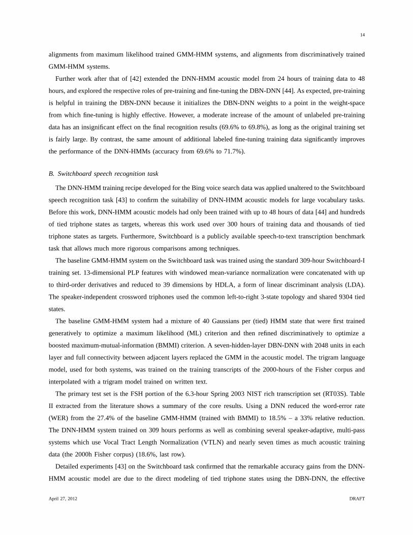
A comparison of the Percentage Word Error Rates using DNN-HMMs and GMM-HMMs on five different large vocabulary tasks.
task hours of DNN-HMM GMM-HMM GMM-HMM
training data with same data with more data
Switchboard (test set 1) 309 18.5 27.4 18.6 (2000 hrs)
Switchboard (test set 2) 309 16.1 23.6 17.1 (2000 hrs)
English Broadcast News 50 17.5 18.8
Bing Voice Search 24 30.4 36.2
(Sentence error rates)
Google Voice Input 5,870 12.3 16.0 (>>5,870hrs)
Youtube 1,400 47.6 52.3
created at IBM use the following recipe to produce a state-of-the-art baseline system. First speaker-independent
(SI) features are created, followed by speaker-adaptivelytrained (SAT) and discriminatively trained (DT) features.
Specifically, given initial PLP features, a set of SI features are created using Linear Discriminative Analysis (LDA).
Further processing of LDA features is performed to create SAT features using vocal tract length normalization
(VTLN) followed by feature space Maximum Likelihood LinearRegression (fMLLR). Finally, feature and model-
space discriminative training is applied using the the Boosted Maximum Mutual Information (BMMI) or Minimum
Phone Error (MPE) criterion.
Using alignments from a baseline system, [32] trained a DBN-DNN acoustic model on 50 hours of data from the
1996 and 1997 English Broadcast News Speech Corpora [37]. The DBN-DNN was trained with the best-performing
LVCSR features, namely SAT + DT features. The DBN-DNN architecture consisted of 6 hidden layers with 1,024
units per layer and a final softmax layer of 2,220 context-dependent states. The SAT+DT feature input into the first
layer used a context of 9 frames. Pre-training was performedfollowing a recipe similar to [42].
Two phases of fine-tuning were performed. During the first phase, the cross-entropy loss was used. For cross-
entropy training, after each iteration through the whole training set, loss is measured on a held-out set and the
learning rate is annealed (i.e. reduced) by a factor of 2 if the held-out loss has grown or improves by less than
a threshold of 0.01% from the previous iteration. Once the learning rate has been annealed five times, the first
phase of fine-tuning stops. After weights are learned via cross-entropy, these weights are used as a starting point
for a second phase of fine-tuning using a sequence criterion [37] which utilizes the MPE objective function, a
discriminative objective function similar to MMI [7] but which takes into account phoneme error rate.
A strong SAT+DT GMM-HMM baseline system, which consisted of2,220 context-dependent states and 50,000
Gaussians, gave a WER of 18.8% on the EARS Dev-04f set, whereasthe DNN-HMM system gave 17.5% [50].
F. Summary of the main results for DBN-DNN acoustic models onLVCSR tasks
Table III summarizes the acoustic modeling results described above. It shows that DNN-HMMs consistently
outperform GMM-HMMs that are trained on the same amount of data, sometimes by a large margin. For some
tasks, DNN-HMMs also outperform GMM-HMMs that are trained on much more data.
April 27, 2012 DRAFT

18
G. Speeding up DNNs at recognition time
State pruning or Gaussian selection methods can be used to make GMM-HMM systems computationally efficient
at recognition time. A DNN, however, uses virtually all its parameters at every frame to compute state likelihoods,
making it potentially much slower than a GMM with a comparable number of parameters. Fortunately, the time that
a DNN-HMM system requires to recognize 1s of speech can be reduced from 1.6s to 210ms, without decreasing
recognition accuracy, by quantizing the weights down to 8 bits and using the very fast SIMD primitives for fixed-
point computation that are provided by a modern x86 CPU[49].Alternatively, it can be reduced to 66ms by using
a GPU.
H. Alternative pre-training methods for DNNs
Pre-training DNNs as generative models led to better recognition results on TIMIT and subsequently on a variety
of LVCSR tasks. Once it was shown that DBN-DNNs could learn good acoustic models, further research revealed
that they could be trained in many different ways. It is possible to learn a DNN by starting with a shallow neural
net with a single hidden layer. Once this net has been traineddiscriminatively, a second hidden layer is interposed
between the first hidden layer and the softmax output units and the whole network is again discriminatively trained.
This can be continued until the desired number of hidden layers is reached, after which full backpropagation
fine-tuning is applied.
This type of discriminative pre-training works well in practice, approaching the accuracy achieved by generative
DBN pre-training and further improvement can be achieved bystopping the discriminative pre-training after a single
epoch instead of multiple epochs as reported in [45]. Discriminative pre-training has also been found effective
for the architectures called “deep convex network” [51] and“deep stacking network” [52], where pre-training is
accomplished by convex optimization involving no generative models.
Purely discriminative training of the whole DNN from randominitial weights works much better than had been
thought, provided the scales of the initial weights are set carefully, a large amount of labeled training data is available,
and mini-batch sizes over training epochs are set appropriately [45], [53]. Nevertheless, generative pre-training still
improves test performance, sometimes by a significant amount.
Layer-by-layer generative pre-training was originally done using RBMs, but various types of autoencoder with
one hidden layer can also be used (see figure 2). On vision tasks, performance similar to RBMs can be achieved
by pre-training with “denoising” autoencoders [54] that are regularized by setting a subset of the inputs to zero
or “contractive” autoencoders [55] that are regularized bypenalizing the gradient of the activities of the hidden
units with respect to the inputs. For speech recognition, improved performance was achieved on both TIMIT and
Broadcast News tasks by pre-training with a type of autoencoder that tries to find sparse codes [56].
I. Alternative fine-tuning methods for DNNs
Very large GMM acoustic models are trained by making use of the parallelism available in compute clusters.
It is more difficult to use the parallelism of cluster systemseffectively when training DBN-DNNs. At present, the
April 27, 2012 DRAFT

19
code units
input units
output units
Fig. 2. An autoencoder is trained to minimize the discrepancy between the input vector and its reconstruction of the input vector on its output
units. If the code units and the output units are both linear and the discrepancy is the squared reconstruction error, an autoencoder finds the
same solution as Principal Components Analysis (up to a rotation of the components). If the output units and the code units are logistic, an
autoencoder is quite similar to an RBM that is trained using contrastive divergence, but it does not work as well for pre-training DNNs unless it
is strongly regularized in an appropriate way. If extra hidden layers are added before and/or after the code layer, an autoencoder can compress
data much better than Principal Components Analysis[17].
most effective parallelization method is to parallelize the matrix operations using a GPU. This gives a speed-up of
between one and two orders of magnitude, but the fine-tuning stage remains a serious bottleneck and more effective
ways of parallelizing training are needed. Some recent attempts are described in [52], [57].
Most DBN-DNN acoustic models are fine-tuned by applying stochastic gradient descent with momentum to
small mini-batches of training cases. More sophisticated optimization methods that can be used on larger mini-
batches include non-linear conjugate-gradient [17], LBFGS [58] and “Hessian Free” methods adapted to work for
deep neural networks [59]. However, the fine-tuning of DNN acoustic models is typically stopped early to prevent
overfitting and it is not clear that the more sophisticated methods are worthwhile for such incomplete optimization.
V. OTHER WAYS OF USING DEEPNEURAL NETWORKS FORSPEECHRECOGNITION
The previous section reviewed experiments in which GMMs were replaced by DBN-DNN acoustic models to
give hybrid DNN-HMM systems in which the posterior probabilities over HMM states produced by the DBN-DNN
replace the GMM output model. In this section, we describe two other ways of using DNNs for speech recognition.
A. Using DBN-DNNs to provide input features for GMM-HMM systems
Here we describe a class of methods where neural networks areused to provide the feature vectors that the
GMM in a GMM-HMM system is trained to model. The most common approach to extracting these feature vectors
is to discriminatively train a randomly initialized neuralnet with a narrow bottleneck middle layer and to use the
activations of the bottleneck hidden units as features. Fora summary of such methods, commonly known as the
tandem approach, see [60], [61].
April 27, 2012 DRAFT

20
Recently, [62] investigated a less direct way of producing feature vectors for the GMM. First, a DNN with
six hidden layers of 1024 units each was trained to achieve good classification accuracy for the 384 HMM states
represented in its softmax output layer. This DNN did not have a bottleneck layer and it was therefore able to
classify better than a DNN with a bottleneck. Then the 384 logits computed by the DNN as input to its softmax
layer were compressed down to 40 values using a 384-128-40-384 autoencoder. This method of producing feature
vectors is called AE-BN because the bottleneck is in the autoencoder rather than in the DNN that is trained to
classify HMM states.
Bottleneck feature experiments were conducted on 50 hours and 430 hours of data from the 1996 and 1997
English Broadcast News Speech collections and English broadcast audio from TDT-4. The baseline GMM-HMM
acoustic model trained on 50 hours was the same acoustic model described in Section IV-E. The acoustic model
trained on 430 hours had 6,000 states and 150,000 Gaussians.Again, the standard IBM LVCSR recipe described
in Section IV-E was used to create a set of speaker-adapted, discriminatively trained features and models.
All DBN-DNNs used SAT features as input. They were pre-trained as DBNs and then discriminatively fine-tuned
to predict target values for 384 HMM states that were obtained by clustering the context-dependent states in the
baseline GMM-HMM system. As in section IV-E, the DBN-DNN wastrained using the cross-entropy criterion,
followed by the sequence criterion with the same annealing and stopping rules.
After the training of the first DBN-DNN terminated, the final set of weights was used for generating the 384
logits at the output layer. A second 384-128-40-384 DBN-DNNwas then trained as an auto-encoder to reduce the
dimensionality of the output logits. The GMM-HMM system that used the feature vectors produced by the AE-BN
was trained using feature and model space discriminative training. Both pre-training and the use of deeper networks
made the AE-BN features work better for recognition. To fairly compare the performance of the system that used
the AE-BN features with the baseline GMM-HMM system, the acoustic model of the AE-BN features was trained
with the same number of states and Gaussians as the baseline system.
Table IV shows the results of the AE-BN and baseline systems on both 50 and 430 hours, for different steps in
the LVCSR recipe described in Section IV-E. On 50 hours, the AE-BN system offers a 1.3% absolute improvement
over the baseline GMM-HMM system which is the same improvement as the DBN-DNN, while on 430 hours the
AE-BN system provides a0.5% improvement over the baseline. The 17.5% WER is the best result to date on the
Dev-04f task, using an acoustic model trained on 50 hours of data. Finally, the complementarity of the AE-BN
and baseline methods is explored by performing model combination on both the 50 and 430 hour tasks. Table IV
shows that model-combination provides an additional1.1% absolute improvement over individual systems on the
50 hour task, and a0.5% absolute improvement over the individual systems on the 430hour task, confirming the
complementarity of the AE-BN and baseline systems.
Instead of replacing the coefficients usually modeled by GMMs, neural networks can also be used to provide
additional features for the GMM to model [8], [9], [63]. DBN-DNNs have recently been shown to be very effective
in such tandem systems. On the Aurora2 test set, pre-training decreased word error rates by more than one third
for speech with signal-to-noise levels of 20dB or more, though this effect almost disappeared for very high noise
April 27, 2012 DRAFT

21
TABLE IV
WER in % on English Broadcast News
50 Hours 430 Hours
LVCSR Stage GMM-HMM Baseline AE-BN GMM/HMM Baseline AE-BN
FSA 24.8 20.6 20.2 17.6
+fBMMI 20.7 19.0 17.7 16.6
+BMMI 19.6 18.1 16.5 15.8
+MLLR 18.8 17.5 16.0 15.5
Model Combination 16.4 15.0
levels [64].
B. Using DNNs to estimate articulatory features for detection-based speech recognition
A recent study [65] demonstrated the effectiveness of DBN-DNNs for detecting sub-phonetic speech attributes
(also known as phonological or articulatory features [66])in the widely used Wall Street Journal speech database
(5k-WSJ0). 13 MFCCs plus first and second temporal derivatives were used as the short-time spectral representation
of the speech signal. The phone labels were derived from the forced alignments generated using a GMM-HMM
system trained with maximum likelihood, and that HMM systemhad 2818 tied-state, cross-word tri-phones, each
modeled by a mixture of 8 Gaussians. The attribute labels were generated by mapping phone labels to attributes,
simplifying the overlapping characteristics of the articulatory features. The 22 attributes used in the recent work,
as reported in [65], are a subset of the articulatory features explored in [66], [67].
DBN-DNNs achieved less than half the error rate of shallow neural nets with a single hidden layer. DNN
architectures with 5 to 7 hidden layers and up to 2048 hidden units per layer were explored, producing greater
than 90% frame-level accuracy for all 21 attributes tested in the full DNN system. On the same data, DBN-DNNs
also achieved a very high per frame phone classification accuracy of 86.6%. This level of accuracy for detecting
sub-phonetic fundamental speech units may allow a new family of flexible speech recognition and understanding
systems that make use of phonological features in the full detection-based framework discussed in [65].
VI. SUMMARY AND FUTURE DIRECTIONS
When GMMs were first used for acoustic modeling they were trained as generative models using the EM algorithm
and it was some time before researchers showed that significant gains could be achieved by a subsequent stage of
discriminative training using an objective function more closely related to the ultimate goal of an ASR system[7],
[68]. When neural nets were first used they were trained discriminatively and it was only recently that researchers
showed that significant gains could be achieved by adding an initial stage of generative pre-training that completely
ignores the ultimate goal of the system. The pre-training ismuch more helpful in deep neural nets than in shallow
ones, especially when limited amounts of labeled training data are available. It reduces overfitting and it also reduces
the time required for discriminative fine-tuning with backpropagation which was one of the main impediments to
using DNNs when neural networks were first used in place of GMMs in the 1990s. The successes achieved using
April 27, 2012 DRAFT

22
pre-training led to a resurgence of interest in DNNs for acoustic modeling. Retrospectively, it is now clear that
most of the gain comes from using deep neural networks to exploit information in neighboring frames and from
modeling tied context-dependent states. Pre-training is helpful in reducing overfitting, and it does reduce the time
taken for fine-tuning, but similar reductions in training time can be achieved with less effort by careful choice of
the scales of the initial random weights in each layer.
The first method to be used for pre-training DNNs was to learn astack of RBMs, one per hidden layer of the
DNN. An RBM is an undirected generative model that uses binary latent variables, but training it by maximum
likelihood is expensive so a much faster, approximate method called contrastive divergence is used. This method has
strong similarities to training an autoencoder network (a non-linear version of PCA) that converts each datapoint
into a code from which it is easy to approximately reconstruct the datapoint. Subsequent research showed that
autoencoder networks with one layer of logistic hidden units also work well for pre-training, especially if they are
regularized by adding noise to the inputs or by constrainingthe codes to be insensitive to small changes in the
input. RBMs do not require such regularization because the Bernoulli noise introduced by using stochastic binary
hidden units acts as a very strong regularizer.
We have described how three major speech research groups achieved significant improvements in a variety
of state-of-the-art ASR systems by replacing GMMs with DNNs, and we believe that there is the potential for
considerable further improvement. There is no reason to believe that we are currently using the optimal types of
hidden units or the optimal network architectures and it is highly likely that both the pre-training and fine-tuning
algorithms can be modified to reduce the amount of overfittingand the amount of computation. We therefore expect
that the performance gap between acoustic models that use DNNs and ones that use GMMs will continue to increase
for some time.
Currently, the biggest disadvantage of DNNs compared with GMMs is that it is much harder to make good use of
large cluster machines to train them on massive datasets. This is offset by the fact that DNNs make more efficient
use of data so they do not require as much data to achieve the same performance, but better ways of parallelizing
the fine-tuning of DNNs is still a major issue.
REFERENCES
[1] J. Baker, L. Deng, J. Glass, S. Khudanpur, Chin hui Lee, N.Morgan, and D. O’Shaughnessy, “Developments and directionsin speech
recognition and understanding, part 1,”Signal Processing Magazine, IEEE, vol. 26, no. 3, pp. 75–80, may 2009.
[2] S. Furui, Digital Speech Processing, Synthesis, and Recognition, Marcel Dekker, 2000.
[3] B. H. Juang, S. Levinson, and M. Sondhi, “Maximum likelihood estimation for multivariate mixture observations of Markovchains,”
IEEE Transactions on Information Theory, vol. 32, no. 2, pp. 307–309, 1986.
[4] H. Hermansky, “Perceptual linear predictive (plp) analysis of speech,”The Journal of the Acoustical Society of America, vol. 87, no. 4,
pp. 1738–1752, 1990.
[5] S. Furui, “Cepstral analysis technique for automatic speaker verification,” IEEE Trans. ASSP, vol. ASSP-29, pp. 254–272, 1981.
[6] S. Young, “Large Vocabulary Continuous Speech Recognition: A Review,” IEEE Signal Processing Magazine, vol. 13, no. 5, pp. 45–57,
1996.
[7] L. Bahl, P. Brown, P. de Souza, and R. Mercer, “Maximum mutual information estimation of hidden Markov model parameters for speech
recognition,” inProceedings of the ICASSP, 1986, pp. 49–52.
April 27, 2012 DRAFT
23
[8] H. Hermansky, D. P. W. Ellis, and S. Sharma, “Tandem connectionist feature extraction for conventional HMM systems,” inProceedings
of ICASSP, Los Alamitos, CA, USA, 2000, vol. 3, pp. 1635–1638, IEEE Computer Society.
[9] H. Bourlard and N. Morgan,Connectionist Speech Recognition: A Hybrid Approach, Kluwer Academic Publishers, Norwell, MA, USA,
1993.
[10] L. Deng, “Computational models for speech production,” in Computational Models of Speech Pattern Processing, pp. 199–213. Springer-
Verlag, New York, 1999.
[11] L. Deng, “Switching dynamic system models for speech articulation and acoustics,” inMathematical Foundations of Speech and Language
Processing, pp. 115–134. Springer-Verlag, New York, 2003.
[12] A. Mohamed, G. Dahl, and G. Hinton, “Deep belief networksfor phone recognition,” inNIPS Workshop on Deep Learning for Speech
Recognition and Related Applications, 2009.
[13] A. Mohamed, G. Dahl, and G. Hinton, “Acoustic modeling using deep belief networks,”IEEE Transactions on Audio, Speech, and
Language Processing,, vol. 20, no. 1, pp. 14–22, jan. 2012.
[14] D. E. Rumelhart, G. E. Hinton, and R. J. Williams, “Learning representations by back-propagating errors,”Nature, vol. 323, no. 6088,
pp. 533–536, 1986.
[15] X. Glorot and Y. Bengio, “Understanding the difficulty of training deep feedforward neural networks,” inProceedings of AISTATS, 2010,
pp. 249–256.
[16] D. C. Ciresan, U. Meier, L. M. Gambardella, and J. Schmidhuber, “Deep, Big, Simple Neural Nets for Handwritten Digit Recognition,”
Neural Computation, vol. 22, pp. 3207–3220, 2010.
[17] G. E. Hinton and R. Salakhutdinov, “Reducing the dimensionality of data with neural networks,”Science, vol. 313, no. 5786, pp. 504–
507, 2006.
[18] H. Larochelle, D. Erhan, A. Courville, J. Bergstra, andY. Bengio, “An empirical evaluation of deep architectures onproblems with many
factors of variation,” inProceedings of the 24th international conference on Machine learning, 2007, pp. 473–480.
[19] J. Pearl,Probabilistic Inference in Intelligent Systems: Networksof Plausible Inference, Morgan Kaufmann, 1988.
[20] G. E. Hinton, “Training products of experts by minimizingcontrastive divergence,”Neural Computation, vol. 14, pp. 1771–1800, 2002.
[21] G. E. Hinton, “A practical guide to training restrictedboltzmann machines,” Tech. Rep. UTML TR 2010-003, Department of Computer
Science, University of Toronto, 2010.
[22] G. E. Hinton, S. Osindero, and Y. Teh, “A fast learning algorithm for deep belief nets,”Neural Computation, vol. 18, pp. 1527–1554,
2006.
[23] T. N. Sainath, B. Ramabhadran, and M. Picheny, “An exploration of large vocabulary tools for small vocabulary phonetic recognition,” in
IEEE Automatic Speech Recognition and Understanding Workshop, 2009.
[24] A. Mohamed, T. N. Sainath, G E. Dahl, B. Ramabhadran, G. E. Hinton, and M. Picheny, “Deep belief networks using discriminative
features for phone recognition,” inProceedings of ICASSP, 2011.
[25] A. Mohamed, G. Hinton, and G. Penn, “Understanding how deep belief networks perform acoustic modelling,” inProceedings of ICASSP,
2012.
[26] Y. Hifny and S. Renals, “Speech recognition using augmented conditional random fields,”IEEE Transactions on Audio, Speech & Language
Processing, vol. 17, no. 2, pp. 354–365, 2009.
[27] A. Robinson, “An application to recurrent nets to phoneprobability estimation,”IEEE Transactions on Neural Networks, vol. 5, no. 2,
pp. 298–305, 1994.
[28] J. Ming and F. J. Smith, “Improved phone recognition usingbayesian triphone models,” inProc. ICASSP, 1998, p. 409412.
[29] L. Deng and D. Yu, “Use of differential cepstra as acoustic features in hidden trajectory modelling for phonetic recognition,” in Proc.
ICASSP, 2007, pp. 445–448.
[30] A. Halberstadt and J. Glass, “Heterogeneous measurements and multiple classifiers for speech recognition,” inProc. ICSLP, 1998.
[31] A. Mohamed, D. Yu, and L. Deng, “Investigation of full-sequence training of deep belief networks for speech recognition,” in Proceedings
of Interspeech, 2010.
[32] T.N. Sainath, B. Ramabhadran, M. Picheny, D. Nahamoo, andD. Kanevsky, “Exemplar-based sparse representation features: From timit
to lvcsr,” Audio, Speech, and Language Processing, IEEE Transactionson, vol. 19, no. 8, pp. 2598 –2613, nov. 2011.
April 27, 2012 DRAFT

24
[33] G. E. Dahl, M. Ranzato, A. Mohamed, and G. E. Hinton, “Phone recognition with the mean-covariance restricted Boltzmannmachine,”
in Advances in Neural Information Processing Systems 23, J. Lafferty, C. K. I. Williams, J. Shawe-Taylor, R.S. Zemel, and A. Culotta,
Eds., 2010, pp. 469–477.
[34] O. Abdel-Hamid, A. Mohamed, H. Jiang, and G. Penn, “Applying convolutional neural networks concepts to hybrid NN-HMMmodel for
speech recognition,” inProceedings of ICASSP, 2012.
[35] X. He, L. Deng, and W. Chou, “Discriminative Learning in Sequential Pattern Recognition — A Unifying Review for Optimization-Oriented
Speech Recognition,”IEEE Signal Processing Magazine, vol. 25, no. 5, pp. 14–36, 2008.
[36] Y. Bengio, R. De Mori, G. Flammia, and F. Kompe, “Global Optimization of a Neural Network - Hidden Markov Model Hybrid,” in
Proceedings of EuroSpeech, 1991.
[37] B. Kingsbury, “Lattice-based Optimization of SequenceClassification Criteria for Neural-Network Acoustic Modeling,” in Proceedings
of ICASSP, 2009, pp. 3761–3764.
[38] R. Prabhavalkar and E. Fosler-Lussier, “Backpropagation training for multilayer conditional random field based phone recognition,” in
Proc. ICASSP ’10, 2010, pp. 5534–5537.
[39] H. Lee, P. Pham, Y. Largman, and A. Ng, “Unsupervised feature learning for audio classification using convolutional deep belief networks,”
in Advances in Neural Information Processing Systems 22, Y. Bengio, D. Schuurmans, J. Lafferty, C. K. I. Williams, and A. Culotta, Eds.,
2009, pp. 1096–1104.
[40] L. Deng, D. Yu, and A. Acero, “Structured speech modeling,” IEEE Transactions on Audio, Speech, and Langauge Processing, vol. 14,
pp. 1492–1504, 2006.
[41] H. Zen, M. Gales, Y. Nankaku, and K. Tokuda, “Product of experts for statistical parametric speech synthesis,”IEEE Transactions on
Audio, Speech, and Language Processing, vol. 20, no. 3, pp. 794–805, March 2012.
[42] G. Dahl, D. Yu, L. Deng, and A. Acero, “Context-Dependent Pre-Trained Deep Neural Networks for Large-Vocabulary Speech Recognition,”
IEEE Transactions on Audio, Speech, and Language Processing,, vol. 20, no. 1, pp. 30–42, jan 2012.
[43] F. Seide, G. Li, and D. Yu, “Conversational speech transcription using context-dependent deep neural networks,” in Proc. Interspeech,
2011, pp. 437–440.
[44] D. Yu, L. Deng, and G. Dahl, “Roles of pre-training and fine-tuning in context-dependent dbn-hmms for real-world speech recognition,”
in NIPS Workshop on Deep Learning and Unsupervised Feature Learning, 2010.
[45] F. Seide, G. Li, X. Chen, and D. Yu, “Feature engineeringin context-dependent deep neural networks for conversational speech
transcription,” inProc. IEEE ASRU, 2011, pp. 24–29.
[46] D. Povey, D. Kanevsky, B. Kingsbury, B. Ramabhadran, G. Saon, and K. Visweswariah, “Boosted mmi for model and feature-space
discriminative training,” inProceedings of ICASSP, 2008.
[47] N. Jaitly, P. Nguyen, A. Senior, and V. Vanhoucke, “An Application of Pretrained Deep Neural Networks To Large Vocabulary
Conversational Speech Recognition,” Tech. Rep. 001, Department of Computer Science, University of Toronto, 2012.
[48] G. Zweig, P. Nguyen, D.V. Compernolle, K. Demuynck, L. Atlas, P. Clark, G. Sell, M. Wang, F. Sha, H. Hermansky, D. Karakos, A. Jansen,
S. Thomas, G.S.V.S. Sivaram, S. Bowman, and J. Kao, “Speech Recognition with Segmental Conditional Random Fields: A summary of
the JHU CLSP 2010 Summer Workshop,” inProc. ICASSP ’11, 2011, pp. 5044–5047.
[49] V. Vanhoucke, A. Senior, and M. Z. Mao, “Improving the speed of neural networks on cpus,” inProc. Deep Learning and Unsupervised
Feature Learning Workshop, NIPS 2011, 2011.
[50] T. N. Sainath, B. Kingsbury, and B. Ramabhadran, “Improvements in using deep belief networks for large vocabulary continuous speech
recognition,” Tech. Rep. UTML TR 2010-003, Technical Report, Speech and Language Algorithm Group, IBM, February 2011.
[51] L. Deng and D. Yu, “Deep convex network: A scalable architecture for speech pattern classification,” inProc. Interspeech, 2011.
[52] L. Deng, D. Yu, and J. Platt, “Scalable stacking and learning for building deep architectures,” inProceedings of ICASSP, 2012.
[53] D. Yu, L. Deng, G. Li, and Seide F, “Discriminative pre-training of deep neural networks,” inU.S. Patent Filing, Nov. 2011.
[54] P. Vincent H..and Larochelle.and I. Lajoie and.Y. Bengio and P.-A. Manzagol, “Stacked denoising autoencoders: learning useful
representations in a deep network with a local denoising criterion,” Journal of Machine Learning Research, vol. 11, pp. 3371–3408,
2010.
[55] S. Rifai, P. Vincent, X. Muller, X. Glorot, and Y. Bengio, “Contracting auto-encoders: Explicit invariance duringfeature extraction,” in
Proceedings of the 28th International Conference on Machine Learning, 2011.
April 27, 2012 DRAFT

25
[56] C. Plahl, T. N. Sainath, B. Ramabhadran, and D. Nahamoo, “Improved pre-training of deep belief networks using sparse encoding
symmetric machines,” inProceedings of ICASSP, 2012.
[57] B. Hutchinson, L. Deng, and D. Yu, “A deep architecture with bilinear modeling of hidden representations: applications to phonetic
recognition,” inProceedings of ICASSP, 2012.
[58] Q. V. Le, J. Ngiam, A. Coates, A. Lahiri, B. Prochnow, and A. Y. Ng, “On optimization methods for deep learning,” inProceedings of
the 28th International Conference on Machine Learning, 2011.
[59] J. Martens, “Deep Learning via Hessian-free Optimization,” in Proceedings of the 27th International Conference on Machine learning,
2010.
[60] N Morgan, “Deep and wide: Multiple layers in automatic speech recognition,” IEEE Transactions on Audio, Speech, and Language
Processing, vol. 20, no. 1, jan. 2012.
[61] Sivaram G. and H. Hermansky, “Sparse multilayer perceptron for phoneme recognition,”IEEE Transactions on Audio, Speech, and
Language Processing, vol. 20, no. 1, jan. 2012.
[62] T. N. Sainath, B. Kingsbury, and B. Ramabhadran, “Auto-encoder bottleneck features using deep belief networks,” inProc. ICASSP 2012,
2012.
[63] N. Morgan, Qifeng Zhu, A. Stolcke, K. Sonmez, S. Sivadas,T. Shinozaki, M. Ostendorf, P. Jain, H. Hermansky, D. Ellis, G. Doddington,
B. Chen, O. Cretin, H. Bourlard, and M. Athineos, “Pushing the envelope - aside [speech recognition],”Signal Processing Magazine,
IEEE, vol. 22, no. 5, pp. 81 – 88, sept. 2005.
[64] O. Vinyals and S.V. Ravuri, “Comparing multilayer perceptron to deep belief network tandem features for robust asr,”in Proceedings of
ICASSP, 2011, pp. 4596–4599.
[65] D. Yu, S. Siniscalchi, L. Deng, and C. Lee, “Boosting attribute and phone estimation accuracies with deep neural networks for detection-
based speech recognition,” inProceedings of ICASSP, 2012.
[66] L. Deng and D. Sun, “A statistical approach to automatic speech recognition using the atomic speech units constructedfrom overlapping
articulatory features,”Journal of the Acoustical Society of America, vol. 85, no. 5, pp. 2702 – 2719, 1994.
[67] J. Sun and L. Deng, “An overlapping-feature based phonological model incorporating linguistic constraints: Applications to speech
recognition,” Journal of the Acoustical Society of America, vol. 111, no. 2, pp. 1086–1101, 2002.
[68] P.C. Woodland and D. Povey, “Large scale discriminativetraining of hidden markov models for speech recognition,”Computer Speech
and Language, vol. 16, pp. 2547, 2002.
PLACE
PHOTO
HERE
Geoffrey Hinton received his Ph.D. from the University of Edinburgh in 1978.He spent five years as a faculty
member at Carnegie-Mellon University, Pittsburgh, PA, and heis currently a Distinguished Professor at the University
of Toronto. He is a fellow of the Royal Society and an honoraryforeign member of the American Academy of Arts and
Sciences. His awards include the David E. Rumelhart Prize, the International Joint Conference on Artificial Intelligence
Research Excellence Award, and the Gerhard Herzberg CanadaGold Medal for Science and Engineering. He was one of
the researchers who introduced the back-propagation algorithm. His other contributions include Boltzmann machines,
distributed representations, time-delay neural nets, mixtures of experts, variational learning, contrastive divergence
learning, and deep belief nets.
April 27, 2012 DRAFT

26
Li Deng received his Ph.D. from the University of Wisconsin-Madison. In 1989, he joined Dept. Electrical and Computer Engineering, University
of Waterloo, Ontario, Canada as an Assistant Professor, where he became a tenured Full Professor in 1996. In 1999, he joined Microsoft Research,
Redmond, WA as a Senior Researcher, where he is currently a Principal Researcher. Since 2000, he has also been an Affiliate Professor in
the Department of Electrical Engineering at University of Washington, Seattle, teaching the graduate course of ComputerSpeech Processing.
Prior to Microsoft Research, he also worked or taught at Massachusetts Institute of Technology, ATR Interpreting Telecommunications Research
Laboratories (Kyoto, Japan), and Hong Kong University of Science and Technology. In the genearl areas of speech recognition, signal processing,
and machine learning, he has published over 300 refereed papers in leading journals and conferences and 3 books. He is a Fellow of the Acoustical
Society of America, a Fellow of the IEEE, a Fellow of ISCA, and is ISCA’s Distinguished Lecturer 2010-2011. He has been granted over 50
patents, and has received awards/honors bestowed by IEEE, ISCA, ASA, Microsoft, and other organizations including thelatest 2011 IEEE SPS
Meritorious Service Award. He served on the Board of Governors of the IEEE Signal Processing Society (2008-2010), and asEditor-in-Chief
for the IEEE Signal Processing Magazine (2009-2011). He is currently the Editor in Chief of IEEE Transactions on Audio, Speech & Language
Processing 2012-2014, and is General Chair of ICASSP-2013.
Dong Yu joined Microsoft Corporation in 1998 and Microsoft Speech Research Group in 2002, where he is a researcher. He holds a Ph.D.
degree in computer science from University of Idaho, an MS degree in computer science from Indiana University at Bloomington, an MS degree
in electrical engineering from Chinese Academy of Sciences,and a BS degree (with honor) in electrical engineering from Zhejiang University
(China). His current research interests include speech processing, robust speech recognition, discriminative training, spoken dialog system, voice
search technology, machine learning, and pattern recognition. He has published more than 90 papers in these areas and is the inventor/coinventor
of more than 40 granted/pending patents. Dr. Dong Yu is currently serving as an associate editor of IEEE transactions on audio, speech, and
language processing (2011-) and has served as an associate editor of IEEE signal processing magazine (2008-2011) and thelead guest editor of
IEEE transactions on audio, speech, and language processing - special issue on deep learning for speech and language processing (2010-2011).
George E. Dahl received a B.A. in computer science, with highest honors, from Swarthmore College and an M.Sc. from the University of
Toronto, where he is currently completing a Ph.D. with a research focus in statistical machine learning. His current main research interest is in
training models that learn many levels of rich, distributed representations from large quantities of perceptual and linguistic data.
Abdel-rahman Mohamed received his B.Sc. and M.Sc. from the Electronics and Communication Engineering Department, Cairo University
in 2004 and 2007. From 2004 he worked in the speech research group at RDI Company, Egypt. He then joined the ESAT-PSI speech group
at the Katholieke Universiteit Leuven, Belgium. In September2008 he started his PhD at the University of Toronto. His research focus is in
developing machine learning techniques to advance human language technologies.
Navdeep Jaitly received his B.A. from Hanover College and M.Math from the University of Waterloo in 2000. After receiving his Masters,
he developed algorithms and statistical methods for analysisof Protoemics data at Caprion Pharmaceuticals in Montreal andat the Pacific
Northwest National Labs in Washington. Since 2008 he has been pursuing a PhD at the University of Toronto. His current interests lie in
Machine Learning, Speech Recognition, Computational Biology and Statistical Methods.
April 27, 2012 DRAFT

27
Andrew Senior Andrew Senior received his PhD from the University of Cambridge and is a Research Scientist at Google. Before joining
Google he worked at IBM Research in the areas of handwriting,audio-visual speech, face and fingerprint recognition as well as video privacy
protection and visual tracking. He edited the book ”PrivacyProtection in Video Surveillance”; coauthored Springer’s”Guide to Biometrics”
and over sixty scientific papers; holds 26 patents and servesas an Associate Editor of Pattern Recognition journal. His research interests range
across speech and pattern recognition, computer vision and visual art.
Vincent Vanhoucke is a research scientist in Google Research, Mountain View, CA, where he manages the speech quality research team. Prior
to that, he was an early employee at Like.com (now part of Google), where he worked on object, face and text recognition technologies. From
1999 to 2005, he was a research scientist in the speech R&D teamat Nuance, Menlo Park, CA. He received his Ph.D. from Stanford University
in 2004 for research in acoustic modeling, and is a graduate from the Ecole Centrale Paris.
Patrick Nguyen is a research scientist in Google Research, Mountain View, CA. Prior to joining Google, he was with Microsoft Research
in Redmond, WA from 2004-2010. Prior to that, he was working atthe Panasonic Speech Technology Laboratory from 2000-2004, in Santa
Barbara, CA. In 1998, he founded a company developing a platform real-time foreign exchange trading. He received his Doctorate degree from
the Swiss Federal Institute for Technology (EPFL) in 2002. His area of expertise revolves around statistical processing of human language, and
in particular speech recognition. He is mostly known for Segmental Conditional Random Fields and Eigenvoices. He served on the organizing
committee of ASRU 2011 and he co-led the 2010 JHU workshop on Speech Recognition. He currently serves on the Speech and Language
Technical Committee of the IEEE Signal Processing Society.
Tara Sainath received her PhD in Electrical Engineering and Computer Science from MIT in 2009. The main focus of her PhD work was in
acoustic modeling for noise robust speech recognition. She joined the Speech and Language Algorithms group at IBM T.J. Watson Research
Center upon completion of her PhD. She organized a Special Session on Sparse Representations at Interspeech 2010 in Japan. In addition, she
has served as a staff reporter for the IEEE Speech and Language Processing Technical Committee (SLTC) Newsletter. She currently holds 15
US patents. Her research interests mainly focus in acoustic modeling, including sparse representations, deep belief networks, adaptation methods
and noise robust speech recognition.
Brian Kingsbury received the B.S. degree (high honor) in electrical engineering from Michigan State University, East Lansing, in 1989 and
the Ph.D. degree in computer science from the University of California, Berkeley, in 1998. Since 1999 he has been a research staff member
in the Human Language Technologies Department, IBM T. J. Watson Research Center, Yorktown Heights, NY. His research interests include
large-vocabulary speech transcription, audio indexing and analytics, and information retrieval from speech. He has contributed to IBM’s entries
in numerous competitive evaluations of speech technology, including Switchboard, SPINE, EARS, Spoken Term Detection, and GALE. From
2009–2011 he served on the Speech and Language Technical Committee of the IEEE Signal Processing Society, and from 2010–2012 he served
as an ICASSP area chair. He is currently an associate editor for IEEE Transactions on Audio, Speech & Language Processing.
April 27, 2012 DRAFT
Top Related