


Languages
Pages
Legal


1!
!Vincent Lepetit!
Crash Course on TensorFlow!

2!
TensorFlow!
Created by Google for easily implementing Deep Networks;!!Library for Python, but can also be used with C and Java;!!Exists for Linux, Mac OSX, Windows;!!Official documentation: https://www.tensorflow.org
3!
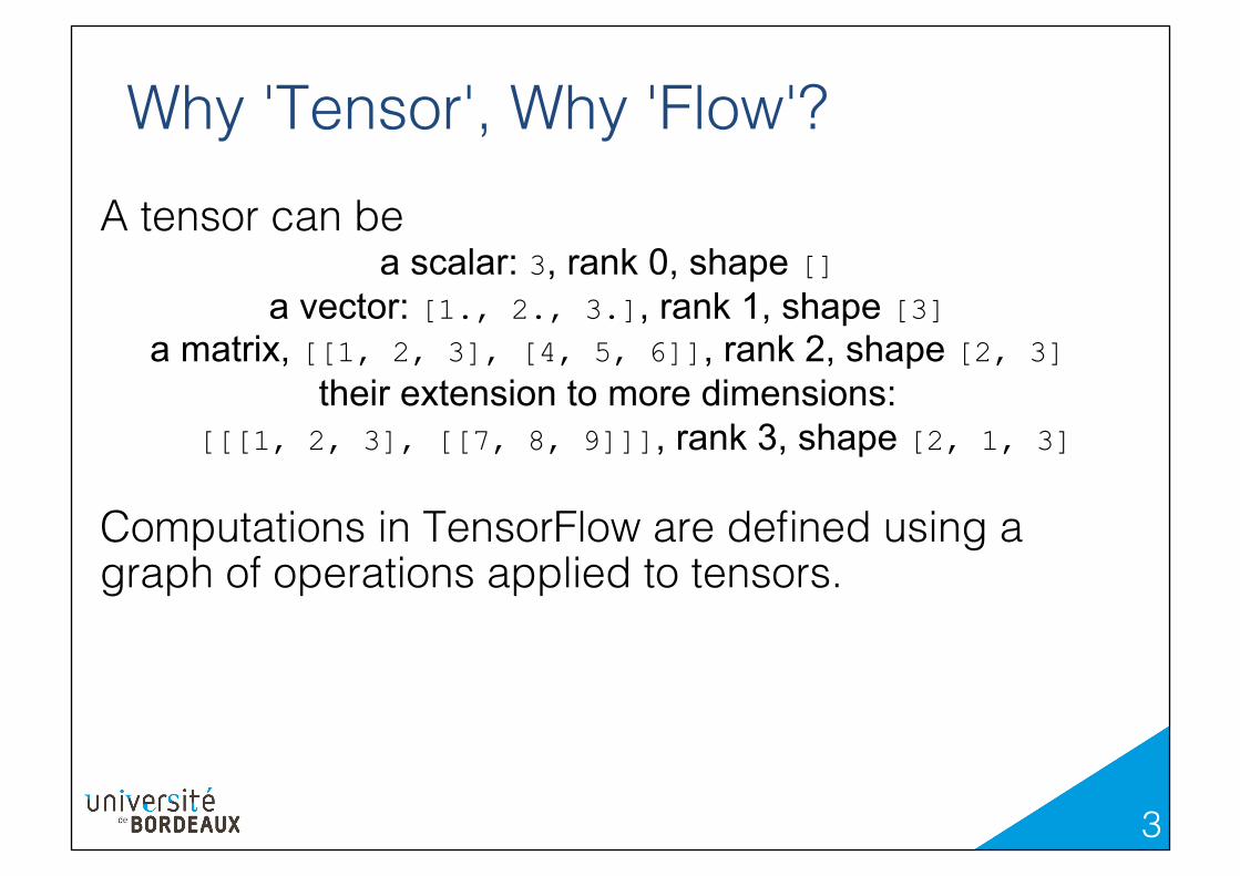
Why 'Tensor', Why 'Flow'?!A tensor can be !
a scalar: 3, rank 0, shape [] a vector: [1., 2., 3.], rank 1, shape [3]
a matrix, [[1, 2, 3], [4, 5, 6]], rank 2, shape [2, 3] their extension to more dimensions:
[[[1, 2, 3], [[7, 8, 9]]], rank 3, shape [2, 1, 3] !Computations in TensorFlow are defined using a graph of operations applied to tensors.!
4!
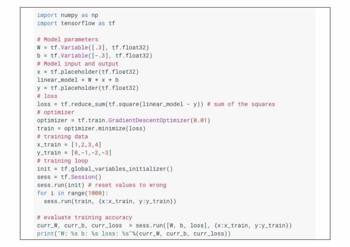
First Full Example:!Linear Regression!
(from the official documentation)!
5!
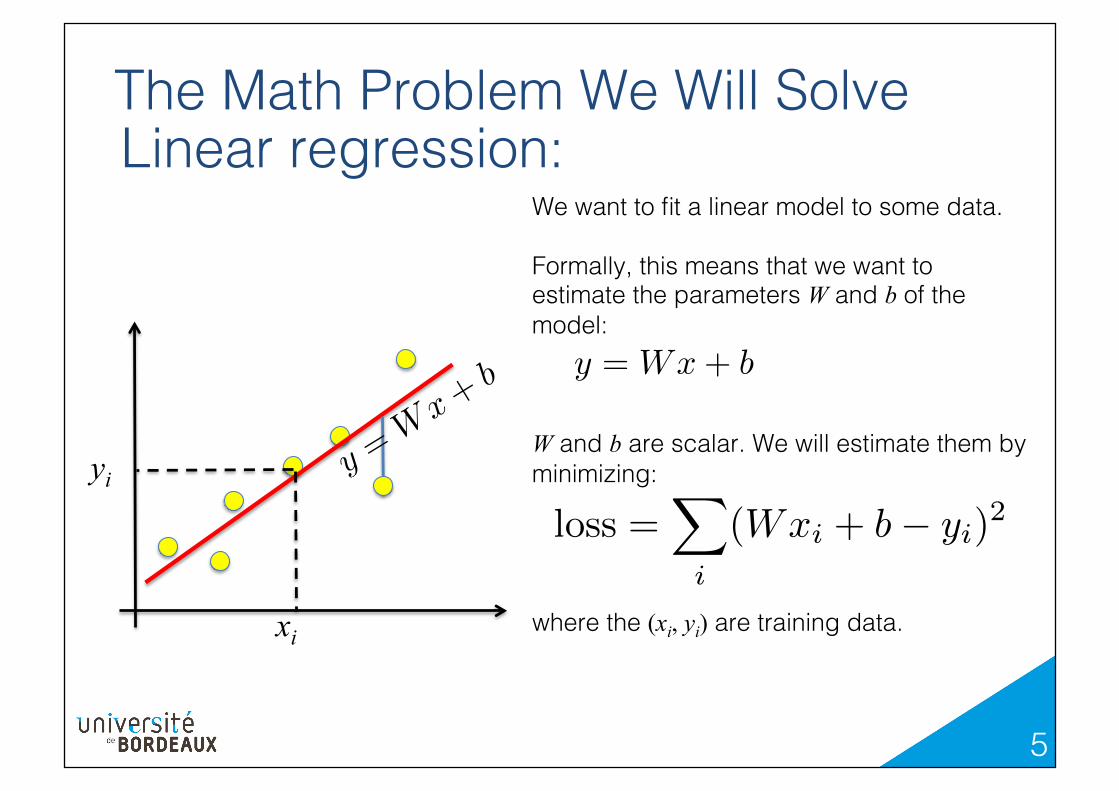
The Math Problem We Will Solve!Linear regression:!
xi
yi
We want to fit a linear model to some data.!!Formally, this means that we want to estimate the parameters W and b of the model:!! !!W and b are scalar. We will estimate them by minimizing:!!!!!where the (xi, yi) are training data.!
loss =
X
i
(Wxi + b� yi)2
y = Wx+ b
y
=W
x
+ b

6!
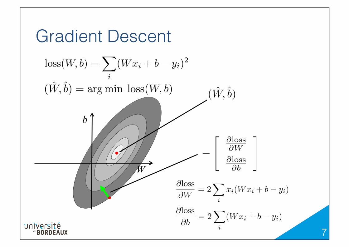
Gradient Descent!
Linear regression can be solved using linear algebra (at least when the problem is small).!!Here we will use gradient descent as this will be a simple example to start with TensorFlow.!
(
ˆW,ˆb) = argmin loss(W, b)
loss(W, b) =
X
i
(Wxi + b� yi)2
7!
Gradient Descent!
(
ˆW,ˆb) = argmin loss(W, b)
loss(W, b) =
X
i
(Wxi + b� yi)2
W
b
(
ˆW,ˆb) = argmin loss(W, b)
�"
@loss@W
@loss@b
#
@loss
@W
= 2
X
i
xi(Wxi + b� yi)
@loss
@b
= 2
X
i
(Wxi + b� yi)
8!
9!
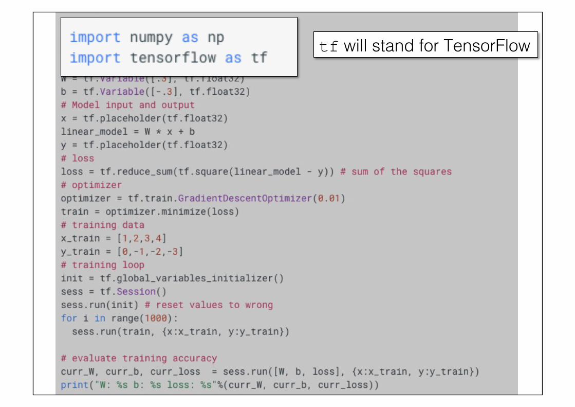
tf will stand for TensorFlow!
10!
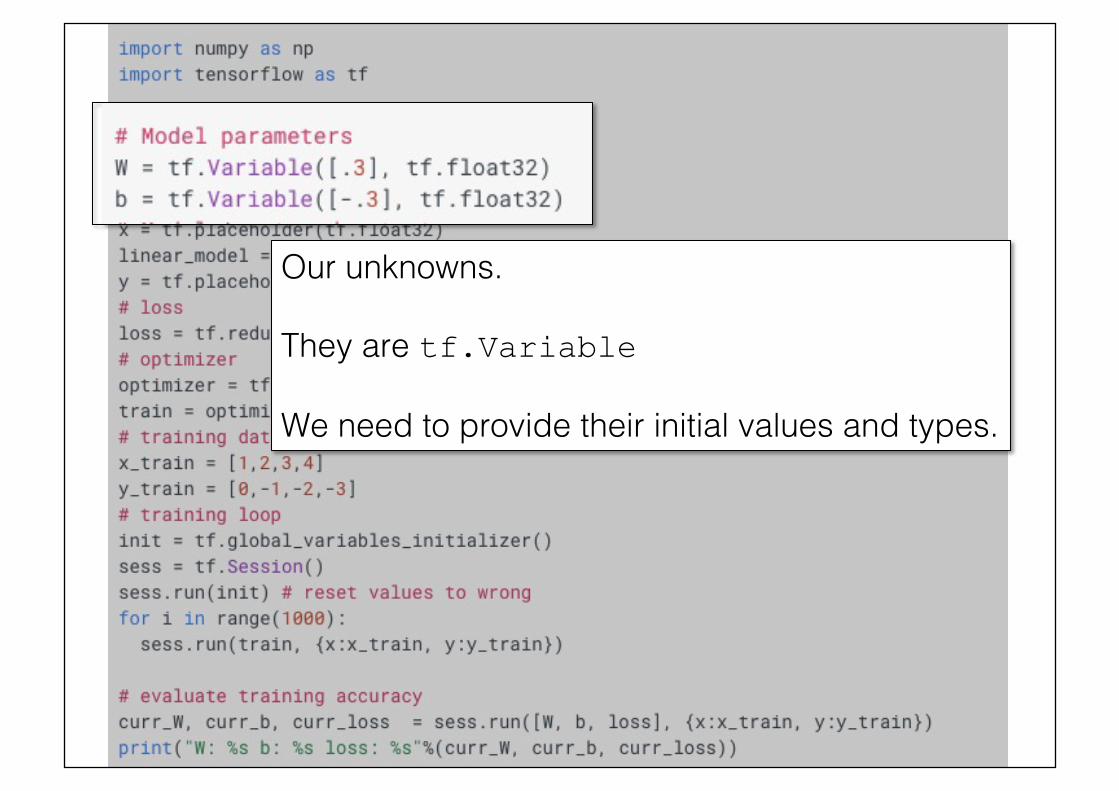
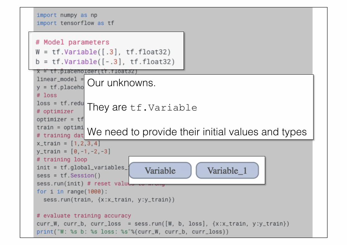
Our unknowns.!!They are tf.Variable !We need to provide their initial values and types.!
11!
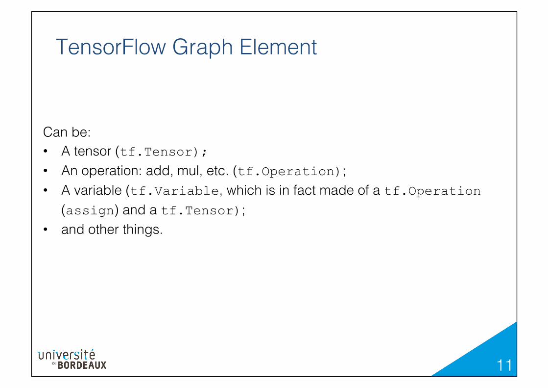
TensorFlow Graph Element !
Can be:!• A tensor (tf.Tensor); !• An operation: add, mul, etc. (tf.Operation);!• A variable (tf.Variable, which is in fact made of a tf.Operation
(assign) and a tf.Tensor);!• and other things.!
12!
Our unknowns.!!They are tf.Variable !We need to provide their initial values and types!
13!
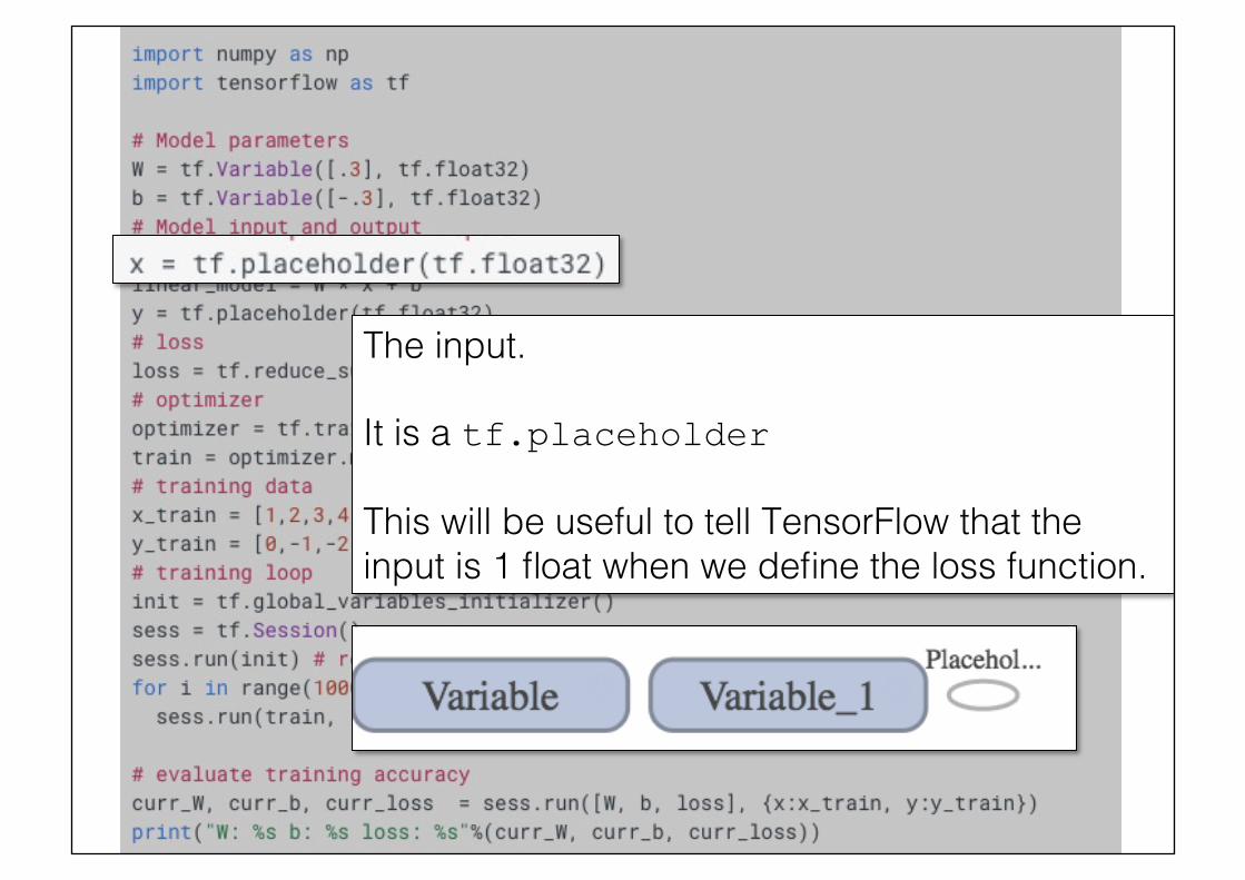
The input.!!It is a tf.placeholder This will be useful to tell TensorFlow that the input is 1 float when we define the loss function.!

14!
linear_model is a tf.Operation It is the predicted output, and will be useful to define the loss function.!
15!
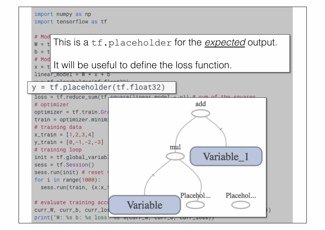
This is a tf.placeholder for the expected output.! It will be useful to define the loss function.!
16!
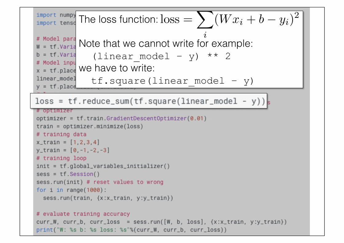
The loss function:! Note that we cannot write for example:! (linear_model – y) ** 2 !we have to write:! tf.square(linear_model – y)
loss =
X
i
(Wxi + b� yi)2

17!

18!
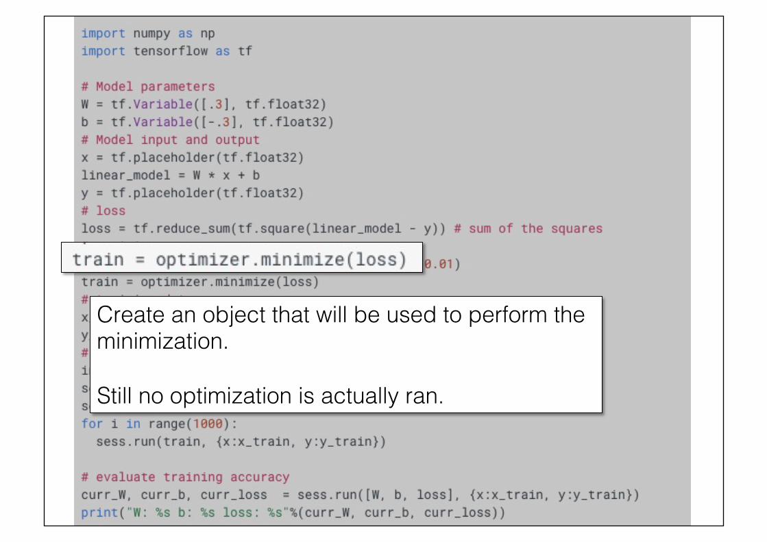
Creates an optimizer object.!!It implements gradient descent.!!0.01 is the step size.
19!
Create an object that will be used to perform the minimization.!!Still no optimization is actually ran.

20!

21!
These are our training data: (1,0), (2, -1), (3, -2), (4, -3)!!They are regular Python arrays.
22!
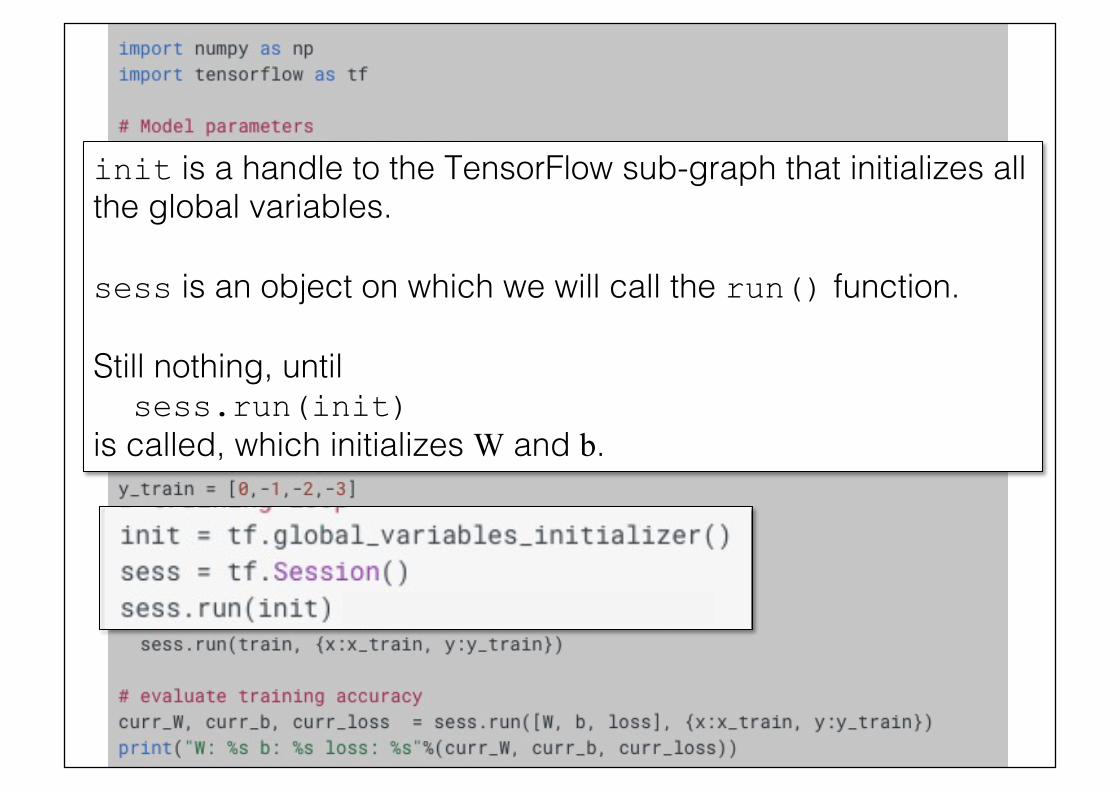
init is a handle to the TensorFlow sub-graph that initializes all the global variables.! sess is an object on which we will call the run() function.!!Still nothing, until! sess.run(init) is called, which initializes W and b.!

23!
24!
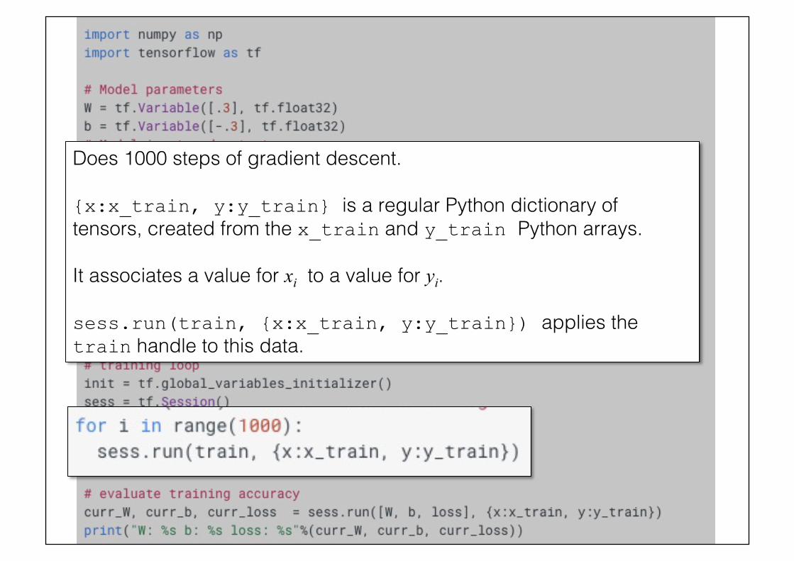
Does 1000 steps of gradient descent.!!{x:x_train, y:y_train} is a regular Python dictionary of tensors, created from the x_train and y_train Python arrays.!!It associates a value for xi to a value for yi.!!sess.run(train, {x:x_train, y:y_train}) applies the train handle to this data.!
25!
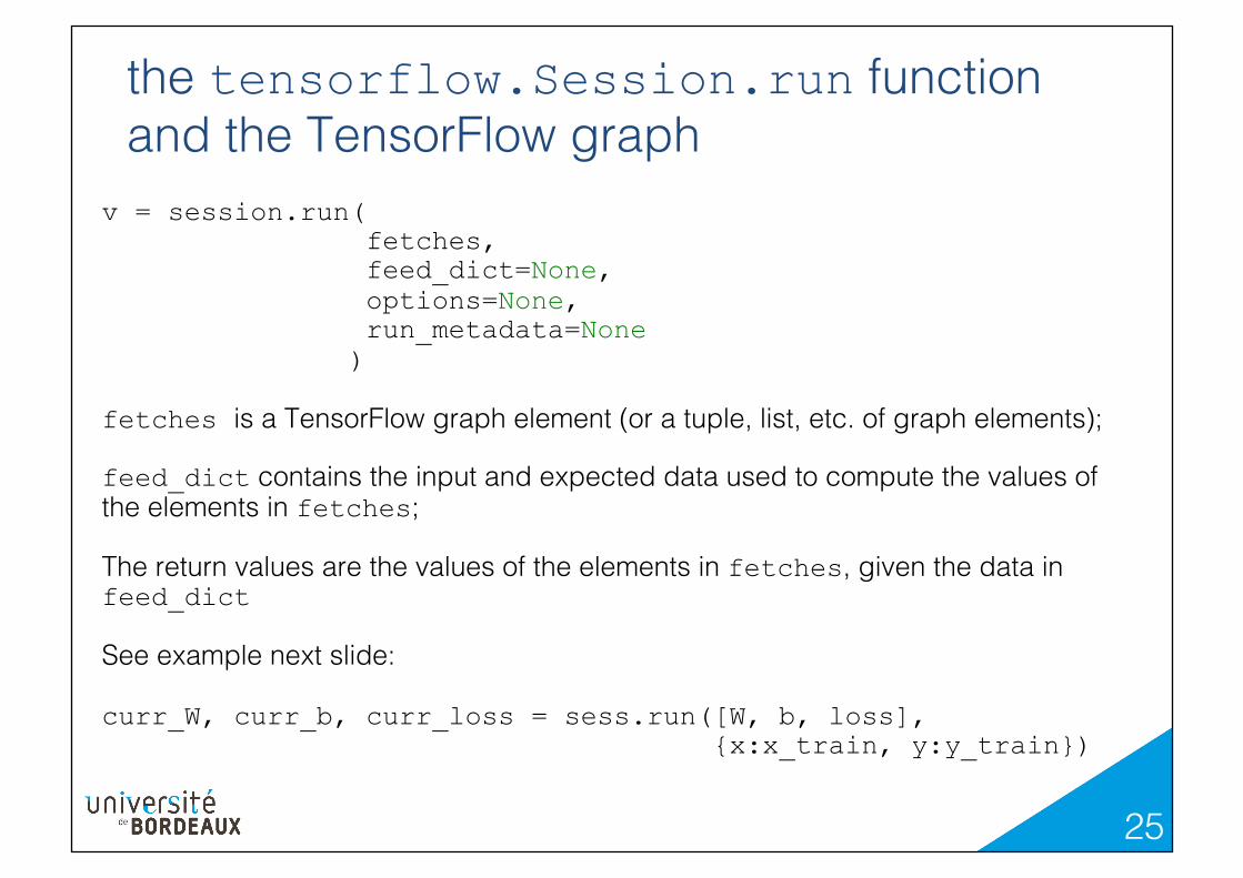
the tensorflow.Session.run function and the TensorFlow graph!
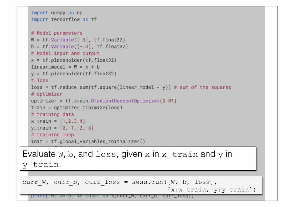
v = session.run( fetches, feed_dict=None, options=None, run_metadata=None ) fetches is a TensorFlow graph element (or a tuple, list, etc. of graph elements);!!feed_dict contains the input and expected data used to compute the values of the elements in fetches;!!The return values are the values of the elements in fetches, given the data in feed_dict !See example next slide:!!curr_W, curr_b, curr_loss = sess.run([W, b, loss], {x:x_train, y:y_train}) !!!!
26!curr_W, curr_b, curr_loss = sess.run([W, b, loss], {x:x_train, y:y_train})
Evaluate W, b, and loss, given x in x_train and y in y_train.

28!
Remark:!!Because linear regression is very common, there is already an object for it. See:!!tf.contrib.learn.LinearRegressor
29!
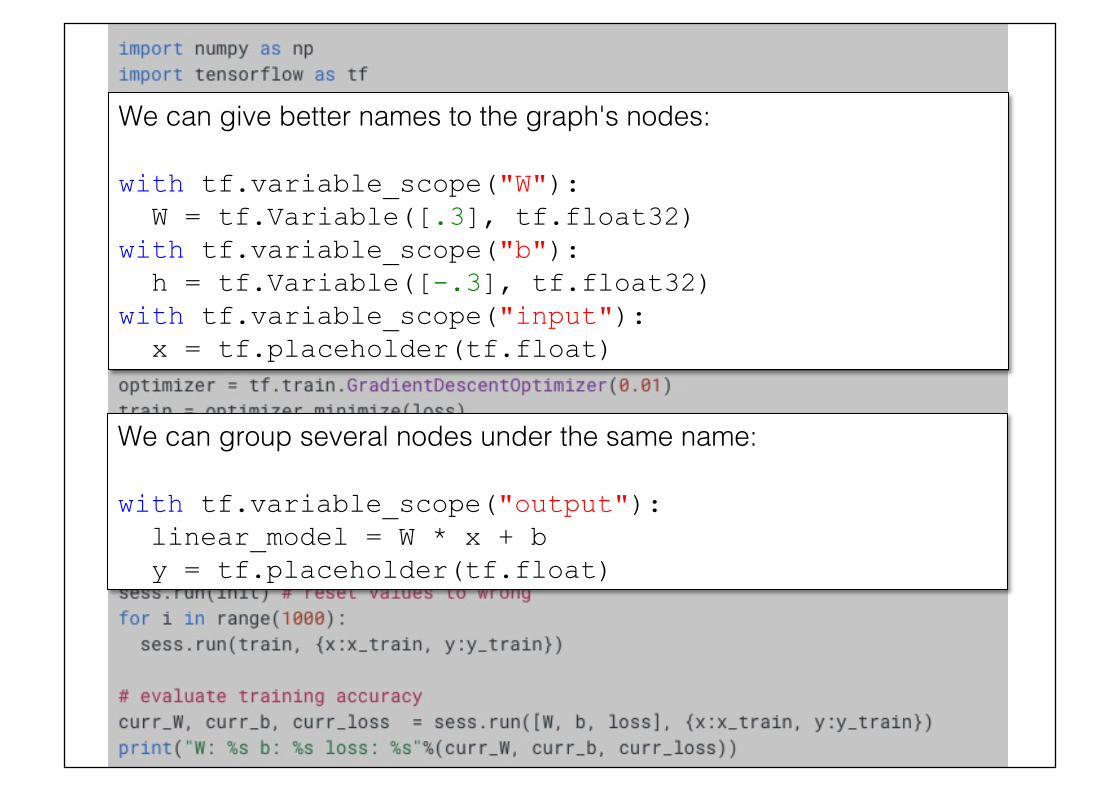
We can give better names to the graph's nodes:! with tf.variable_scope("W"): W = tf.Variable([.3], tf.float32) with tf.variable_scope("b"): h = tf.Variable([-.3], tf.float32) with tf.variable_scope("input"): x = tf.placeholder(tf.float)
We can group several nodes under the same name:! with tf.variable_scope("output"): linear_model = W * x + b y = tf.placeholder(tf.float)
30!
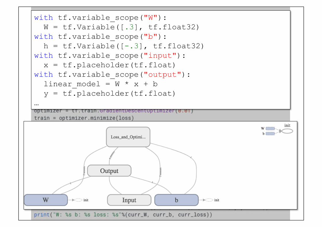
with tf.variable_scope("W"): W = tf.Variable([.3], tf.float32) with tf.variable_scope("b"): h = tf.Variable([-.3], tf.float32) with tf.variable_scope("input"): x = tf.placeholder(tf.float) with tf.variable_scope("output"): linear_model = W * x + b y = tf.placeholder(tf.float) …

31!
Second Example:!Two-Layer Network!
32!
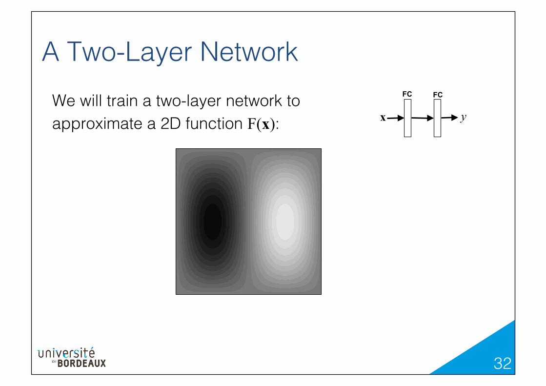
A Two-Layer Network!FC FC
x y We will train a two-layer network to approximate a 2D function F(x):!
33!
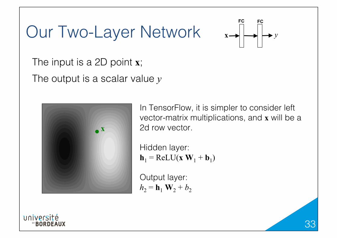
Our Two-Layer Network!FC FC
x y
The input is a 2D point x;!The output is a scalar value y
x
In TensorFlow, it is simpler to consider left vector-matrix multiplications, and x will be a 2d row vector.!!Hidden layer:!h1 = ReLU(x W1 + b1) !Output layer:!h2 = h1 W2 + b2

34!
Loss function!Training set:
Loss =
(x_traini , y_traini)
1
Ns
NsX
i=1
�h2(x train)� y traini
�2
Hidden layer:!h1 = ReLU(x W1 + b1) !Output layer:!h2 = h1 W2 + b2

35!
Generating Training Data!

36!
Defining the Network!FC FC
x y Hidden layer: h1 = ReLU(x W1 + b1) Output layer: h2 = h1 W2 + b2
Loss = 1
Ns
NsX
i=1
�h2(x train)� y traini
�2

37!
Running the Optimization!
Note the generation of the random batch: This is done by keeping the batch_size first elements of the np.random.permutation function !

38!
Visualizing the Predicted Function!without using the run() function!

39!
visualize_2layers() !
h1 = ReLU(x W1 + b1) h2 = h1 W2 + b2

40!
Third Example:!Linear Classification on MNIST!
41!
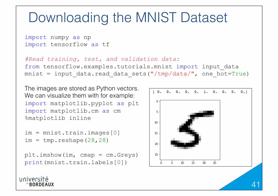
Downloading the MNIST Dataset!import numpy as np import tensorflow as tf #Read training, test, and validation data: from tensorflow.examples.tutorials.mnist import input_data mnist = input_data.read_data_sets("/tmp/data/", one_hot=True) The images are stored as Python vectors. !We can visualize them with for example:!import matplotlib.pyplot as plt import matplotlib.cm as cm %matplotlib inline im = mnist.train.images[0] im = tmp.reshape(28,28) plt.imshow(im, cmap = cm.Greys) print(mnist.train.labels[0])

42!
Model!
with !softmax(h)i =
exphiPj exphj
y = softmax(xW + b)
43!
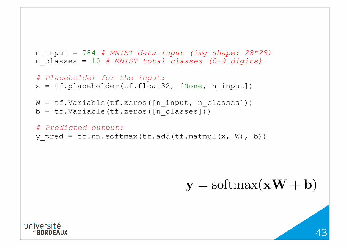
n_input = 784 # MNIST data input (img shape: 28*28) n_classes = 10 # MNIST total classes (0-9 digits) # Placeholder for the input: x = tf.placeholder(tf.float32, [None, n_input]) W = tf.Variable(tf.zeros([n_input, n_classes])) b = tf.Variable(tf.zeros([n_classes])) # Predicted output: y_pred = tf.nn.softmax(tf.add(tf.matmul(x, W), b))
y = softmax(xW + b)
44!
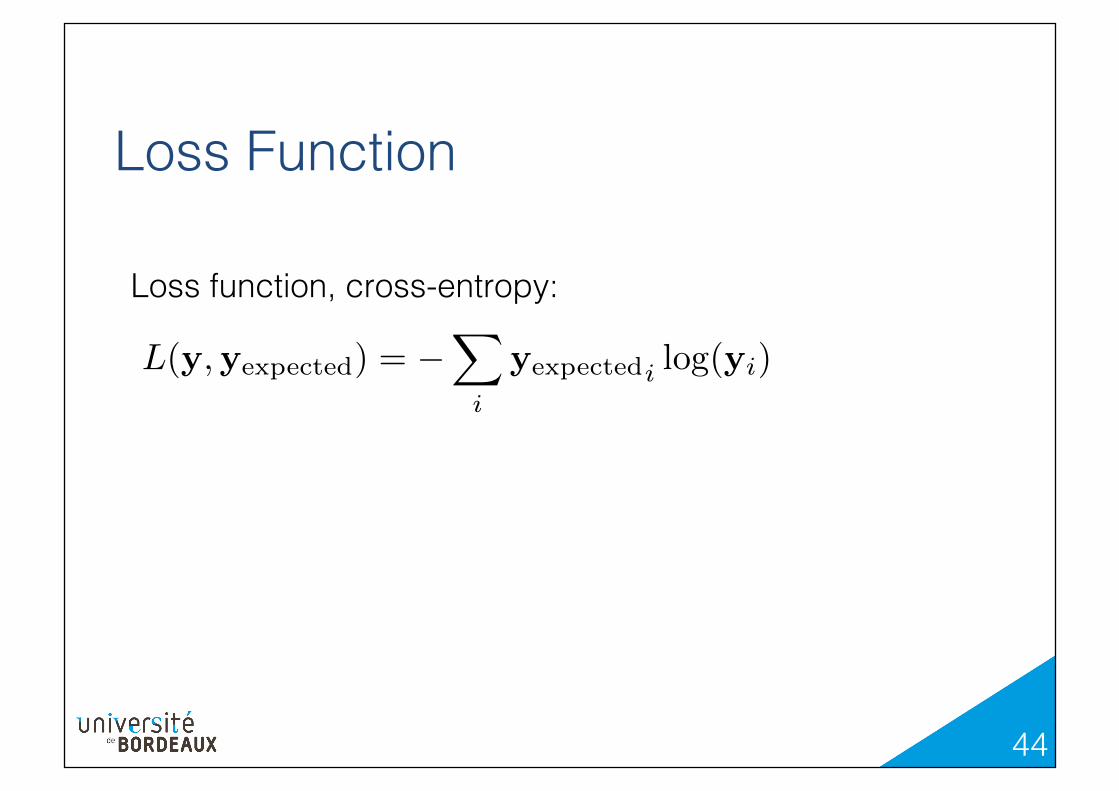
Loss Function!
Loss function, cross-entropy:!!! L(y,y
expected
) = �X
i
yexpectedi log(yi)

45!
# Loss function: cross_entropy = tf.reduce_mean( -tf.reduce_sum( y_exp * tf.log(y_pred), reduction_indices=[1] ) )
L(y,yexpected
) = �X
i
yexpectedi log(yi)
46!
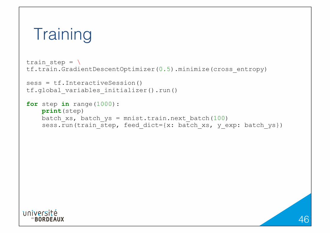
Training!train_step = \ tf.train.GradientDescentOptimizer(0.5).minimize(cross_entropy) sess = tf.InteractiveSession() tf.global_variables_initializer().run() for step in range(1000): print(step) batch_xs, batch_ys = mnist.train.next_batch(100) sess.run(train_step, feed_dict={x: batch_xs, y_exp: batch_ys})

47!
Testing!correct_prediction = tf.equal(tf.argmax(y_pred,1), tf.argmax(y_exp,1)) accuracy = tf.reduce_mean(tf.cast(correct_prediction, tf.float32)) print(sess.run(accuracy, feed_dict={x: mnist.test.images, \ y_exp: mnist.test.labels}))

48!
Visualizing the Model!(after optimization)!
W_array = W.eval(sess) #First column of W: I = W_array.flatten()[0::10].reshape((28,28)) plt.imshow(I, cmap = cm.Greys)

49!
Visualizing the Model!During Optimization!
TensorFlow comes with TensorBoard, a program that can display data saved using TensorFlow functions on a browser.!!To visualize the columns of W during optimization with TensorBoard, we need to:!!1. create a Tensor that contains these columns as an image. This will be done by our
function display_W;!
2. tell TensorFlow that this Tensor is an image and part of a 'summary': A 'summary' is made of data useful for monitoring the optimization, and made to be read by TensorBoard.!
3. create a FileWriter object.!
4. during optimization, we can save the image of the columns using the FileWriter object, and visualize the images using TensorBoard.!
!
50!
display_W( )

51!
Third Example:!A Convolutional Neural Network!
52!
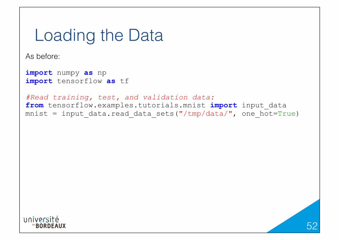
Loading the Data!As before:! import numpy as np import tensorflow as tf #Read training, test, and validation data: from tensorflow.examples.tutorials.mnist import input_data mnist = input_data.read_data_sets("/tmp/data/", one_hot=True)
53!
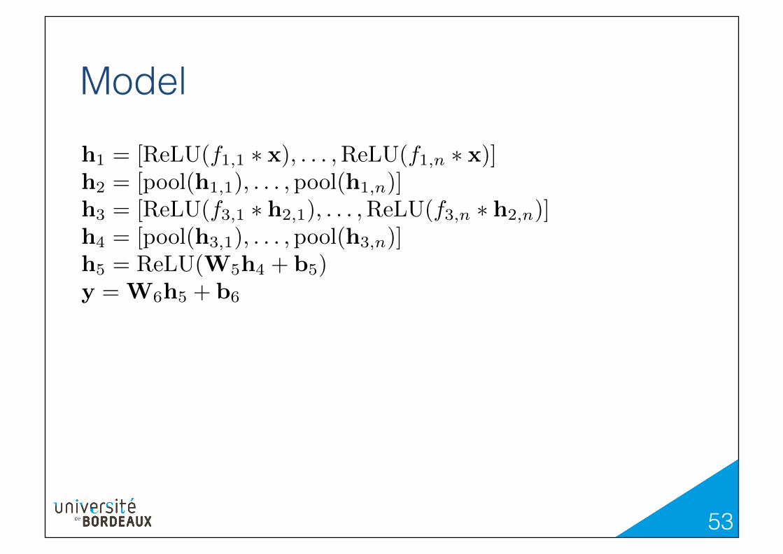
Model!h1 = [ReLU(f1,1 ⇤ x), . . . ,ReLU(f1,n ⇤ x)]h2 = [pool(h1,1), . . . , pool(h1,n)]
h3 = [ReLU(f3,1 ⇤ h2,1), . . . ,ReLU(f3,n ⇤ h2,n)]
h4 = [pool(h3,1), . . . , pool(h3,n)]
h5 = ReLU(W5h4 + b5)
y = W6h5 + b6

54!
n_input = 784 # MNIST data input (img shape: 28*28) n_classes = 10 # MNIST total classes (0-9 digits) #Placeholder for the input: x = tf.placeholder(tf.float32, [None, n_input]) #images are stored as vectors, we reshape them as images: im = tf.reshape(x, shape=[-1, 28, 28, 1]) # 28x28 = 784
We Need to Convert !the Input Vectors into Images!

55!
#32 convolutional 5x5 filters and biases on the first layer: # Filters and biases are initialized # using values drawn from a normal distribution: F1 = tf.Variable(tf.random_normal([5, 5, 1, 32])) b1 = tf.Variable(tf.random_normal([32])) F1_im = tf.nn.conv2d(im, F1, strides=[1, 1, 1, 1],\ padding='SAME') h1 = tf.nn.relu( tf.nn.bias_add(F1_im, b1) )
First Convolutional Layer!h1 = [ReLU(f1,1 ⇤ x), . . . ,ReLU(f1,n ⇤ x)]h2 = [pool(h1,1), . . . , pool(h1,n)]
h3 = [ReLU(f3,1 ⇤ h2,1), . . . ,ReLU(f3,n ⇤ h2,n)]
h4 = [pool(h3,1), . . . , pool(h3,n)]
h5 = ReLU(W5h4 + b5)
y = W6h5 + b6
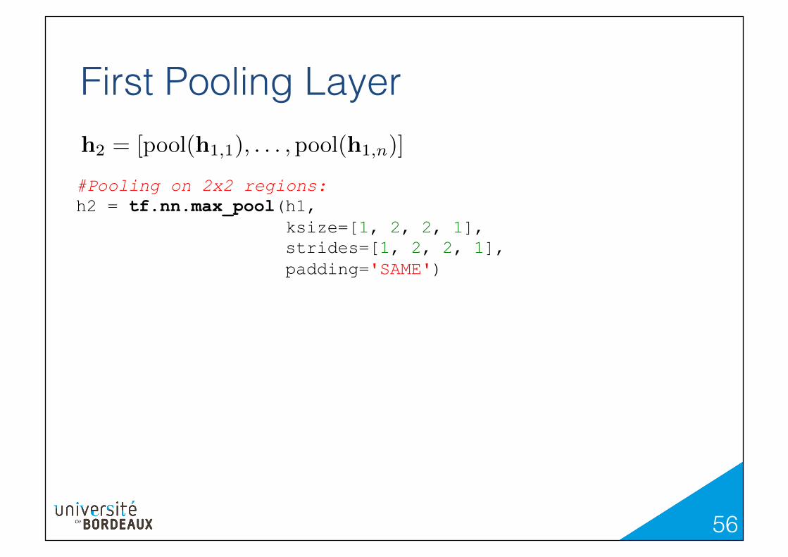
56!
#Pooling on 2x2 regions: h2 = tf.nn.max_pool(h1, ksize=[1, 2, 2, 1], strides=[1, 2, 2, 1], padding='SAME')
First Pooling Layer!h1 = [ReLU(f1,1 ⇤ x), . . . ,ReLU(f1,n ⇤ x)]h2 = [pool(h1,1), . . . , pool(h1,n)]
h3 = [ReLU(f3,1 ⇤ h2,1), . . . ,ReLU(f3,n ⇤ h2,n)]
h4 = [pool(h3,1), . . . , pool(h3,n)]
h5 = ReLU(W5h4 + b5)
y = W6h5 + b6
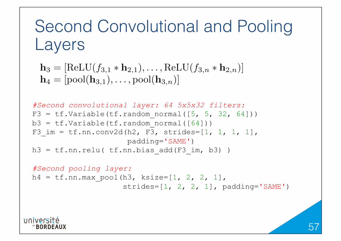
57!
#Second convolutional layer: 64 5x5x32 filters: F3 = tf.Variable(tf.random_normal([5, 5, 32, 64])) b3 = tf.Variable(tf.random_normal([64])) F3_im = tf.nn.conv2d(h2, F3, strides=[1, 1, 1, 1], padding='SAME') h3 = tf.nn.relu( tf.nn.bias_add(F3_im, b3) ) #Second pooling layer: h4 = tf.nn.max_pool(h3, ksize=[1, 2, 2, 1], strides=[1, 2, 2, 1], padding='SAME')
Second Convolutional and Pooling Layers!h1 = [ReLU(f1,1 ⇤ x), . . . ,ReLU(f1,n ⇤ x)]h2 = [pool(h1,1), . . . , pool(h1,n)]
h3 = [ReLU(f3,1 ⇤ h2,1), . . . ,ReLU(f3,n ⇤ h2,n)]
h4 = [pool(h3,1), . . . , pool(h3,n)]
h5 = ReLU(W5h4 + b5)
y = W6h5 + b6

58!
#First fully connected layer, 1024 output: h4_vect = tf.reshape(h4, [-1, 7*7*64]) W5 = tf.Variable(tf.random_normal([7*7*64, 1024])) b5 = tf.Variable(tf.random_normal([1024])) h5 = tf.nn.relu( tf.add(tf.matmul(h4_vect, W5), b5 )) #Second fully connected layer, 1024 input, 10 output: W6 = tf.Variable(tf.random_normal([1024, n_classes])) b6 = tf.Variable(tf.random_normal([n_classes])) #Final predicted output: y_pred = tf.add(tf.matmul(h5, W6), b6) #Placeholder for the expected output: y_exp = tf.placeholder(tf.float32, [None, n_classes])
Two Fully Connected Layers!h1 = [ReLU(f1,1 ⇤ x), . . . ,ReLU(f1,n ⇤ x)]h2 = [pool(h1,1), . . . , pool(h1,n)]
h3 = [ReLU(f3,1 ⇤ h2,1), . . . ,ReLU(f3,n ⇤ h2,n)]
h4 = [pool(h3,1), . . . , pool(h3,n)]
h5 = ReLU(W5h4 + b5)
y = W6h5 + b6

59!
loss = tf.reduce_mean( tf.nn.softmax_cross_entropy_with_logits( logits=y_pred, labels=y_exp ) ) optimizer = tf.train.AdamOptimizer(learning_rate=0.001).minimize(loss) sess = tf.InteractiveSession() tf.global_variables_initializer().run()
Two Fully Connected Layers!

60!
step = 1 training_iters = 20000000 batch_size = 128 # Keep training until reach max iterations while step * batch_size < training_iters: batch_x, batch_y = mnist.train.next_batch(batch_size) sess.run(optimizer, feed_dict={x: batch_x, y_exp: batch_y}) step += 1
Optimization!
61!
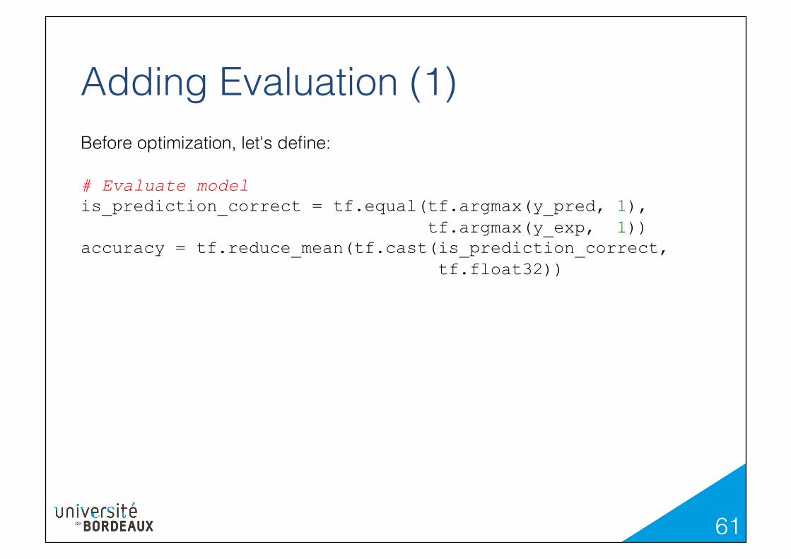
Adding Evaluation (1)!Before optimization, let's define:!!# Evaluate model is_prediction_correct = tf.equal(tf.argmax(y_pred, 1), tf.argmax(y_exp, 1)) accuracy = tf.reduce_mean(tf.cast(is_prediction_correct, tf.float32)) !!
62!
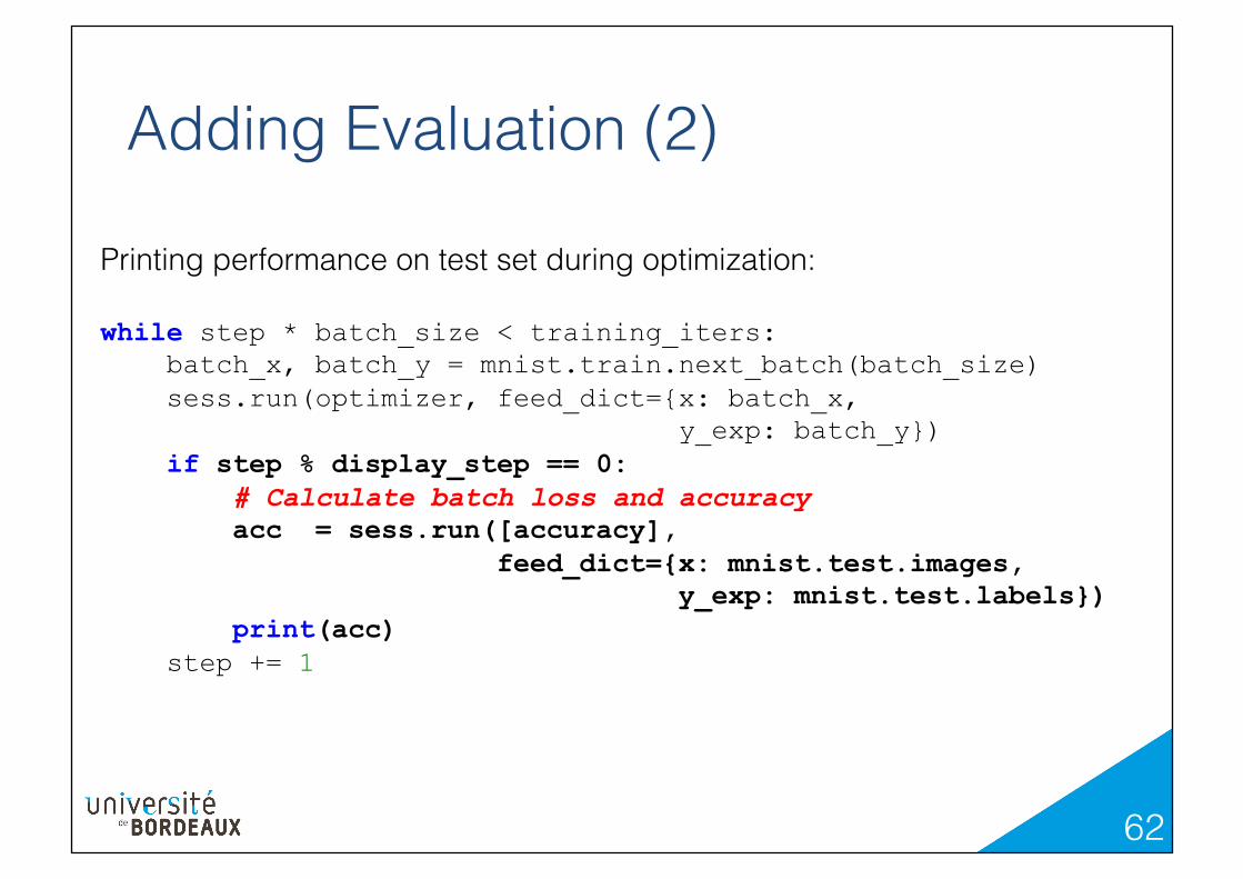
Adding Evaluation (2)!
Printing performance on test set during optimization:!!while step * batch_size < training_iters: batch_x, batch_y = mnist.train.next_batch(batch_size) sess.run(optimizer, feed_dict={x: batch_x, y_exp: batch_y}) if step % display_step == 0: # Calculate batch loss and accuracy acc = sess.run([accuracy], feed_dict={x: mnist.test.images, y_exp: mnist.test.labels}) print(acc) step += 1
63!
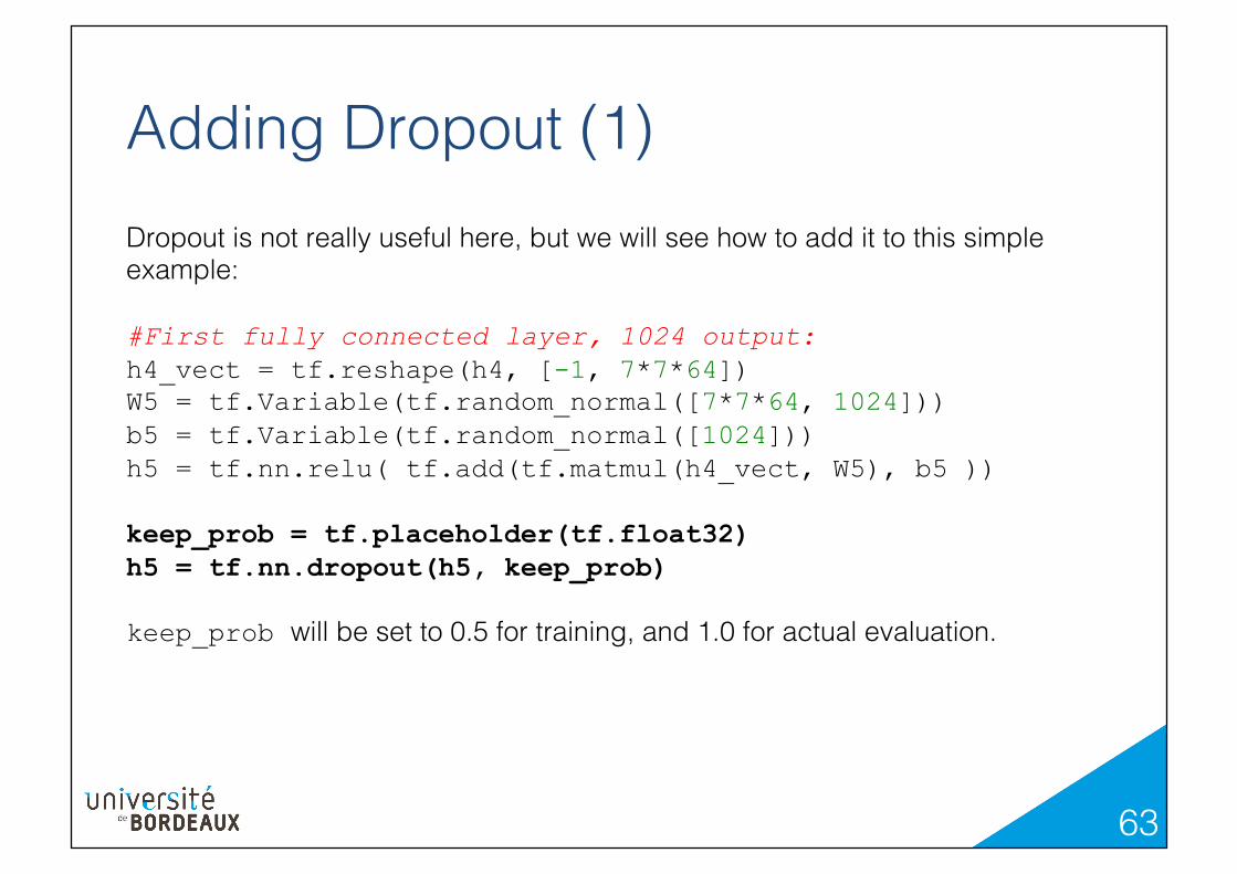
Adding Dropout (1)!Dropout is not really useful here, but we will see how to add it to this simple example:! #First fully connected layer, 1024 output: h4_vect = tf.reshape(h4, [-1, 7*7*64]) W5 = tf.Variable(tf.random_normal([7*7*64, 1024])) b5 = tf.Variable(tf.random_normal([1024])) h5 = tf.nn.relu( tf.add(tf.matmul(h4_vect, W5), b5 )) keep_prob = tf.placeholder(tf.float32) h5 = tf.nn.dropout(h5, keep_prob) keep_prob will be set to 0.5 for training, and 1.0 for actual evaluation.!

64!
# Keep training until reach max iterations while step * batch_size < training_iters: batch_x, batch_y = mnist.train.next_batch(batch_size) # Optimization: sess.run(optimizer, feed_dict={x: batch_x, y_exp: batch_y, keep_prob: 0.5}) # Evaluation: if step % display_step == 0: # Calculate batch loss and accuracy acc = sess.run([accuracy], feed_dict={x: mnist.test.images, y_exp: mnist.test.labels, keep_prob: 1.0} ) print(acc) step += 1
Adding Dropout (2)!
Top Related