Limiting Behavior of Eigenvalues in High-DimensionalMANOVA via RMT

Zhidong Bai1, Kwok Pui Choi2 and Yasunori Fujikoshi3

1School of Mathematics and Statistics and KLAS, Northeast NormalUniversity, Changchun, Jilin 130024, China

2Department of Statistics and Applied Probability, National University ofSingapore, 6 Science Drive 2, 117546, Singapore

3Department of Mathematics, Graduate School of Science, HiroshimaUniversity, Higashi Hiroshima, Hiroshima 739-8626, Japan

Abstract

In this paper we derive the asymptotic joint distributionsof the eigenvalues under the null case in MANOVA model andmultiple discriminant analysis when both the dimension and thesample size are large. Our results are obtained by random matrixtheory (RMT) without assuming normality in the populations. Itis worth pointing out that the null distributions of the eigenval-ues and related test statistics are asymptotically robust againstdeparture from normality in high-dimensional situations. Somenew formulas in RMT are also presented.

AMS 2000 Subject Classification: primary 62H10; secondary 62E20

Key Words and Phrases: Asymptotic distribution, eigenvalues,discriminant analysis, high-dimensional case, MANOVA, nonnor-mality, RMT, test statistics.

Abbreviated title: Limiting Behavior in MANOVA with High-Dimension

1

1 Introduction

It is both basic and important to study the distributions of the eigenvaluesin a one-way multivariate analysis of variance (MANOVA) model. Supposethere are q + 1 groups and {xi1, . . . ,xini

} represents a random sample ofp-vectors from the i-th group, which has mean vector µi and common co-variance matrix Σ. Various inferential procedures are based on the matrices

Sb =1

n

q+1∑i=1

ni(xi − x)(xi − x)′, Se =1

n

q+1∑i=1

ni∑j=1

(xij − xi)(xij − xi)′,

where

xi =1

ni

ni∑j=1

xij, x =1

n

q+1∑i=1

nixi, n =q+1∑i=1

ni.

The matrices nSb and nSe are called the matrices of sums of squares andproducts due to between-groups and within-groups, respectively. Let St =Sb + Se, then nSt is called the matrix of sums of squares and products dueto total variation. These matrices are also used in canonical discriminantanalysis, which is a statistical procedure designed to discriminate betweenseveral different groups in terms of a few discriminant functions.

The large-sample asymptotic distributions of the eigenvalues of SbS−1e or

SbS−1t were derived under normality by Hsu (1941) and Anderson (1951).

A gap in the proof of the main Theorem in Hsu (1941) was corrected byBai (1985). Amemiya (1990) characterised the limiting distributions of theroots of a general determinantal equation. Hsu’s results were extended toasymptotic expansions by a number of authors, see, Sugiura (1976), Fu-jikoshi (1977), Muirhead (1978, 1982), Glynn and Muirhead (1978), etc. Forextension to elliptical case with different covariance matrices, see Seo, Kandaand Fujikoshi (1994).

As is well known, the accuracy of large sample approximations deterioratesas the dimension increases (see, for instance, Bai and Saranadasa (1996)). Asan alternative approach to overcome this shortcoming, it has been consideredto derive asymptotic distributions of the eigenvalues in a high-dimensionalsituation where the dimension p, the sample size n and the number of groupsq + 1 are large. The high-dimensional asymptotic results when p/n → c ∈

2

(0, 1) were obtained (Fujikoshi et al. (2008)) by assuming that the populationeigenvalues are simple. Johnstone (2008) derived the limiting distribution ofthe largest eigenvalue when q/n→ c ∈ (0, 1) in addition to p/n→ c ∈ (0, 1)under the assumption that all the population eigenvalues are zero, i.e., underthe null case. All these results were obtained under normality assumption ofthe populations.

In this paper we derive asymptotic joint distributions of the eigenvalues underthe null case in MANOVA model and multiple discriminant analysis whenboth the dimension and the sample size are large. Our results are obtainedwithout assuming normality via random matrix theory (RMT). There areseveral asymptotic results based on RMT, see, for instances, Bai, Jiang, Yaoand Zheng (2009), Bai, Liu and Wong (2011), Zheng (2012), etc. In this pa-per, we show that by applying RMT, it is possible to derive the asymptoticdistributions of the eigenvalues without assuming normality. In the courseof derivation, we obtain some new limit theorems which may be of indepen-dent interests. It is worth pointing out that our asymptotic results coincidewith those under normality assumption. Therefore some MANOVA tests,including likelihood ratio criterion, Lawley-Hotelling criterion and Bartlett-Nanda-Pillai criterion, are robust against departure from normality when thedimension and the sample size are large.

The organization of the paper is as follows. In Section 2 we state our mainresults (Theorem 2.4 and Corollary 2.1) on the limiting joint distributionsof the nonzero eigenvalues of SbS

−1t and SbS

−1e followed by application to

null robustness of some multivariate tests. In the same section, we alsohighlight some limit theorems which are of independent interests. The proofof Theorem 2.4 is given in Section 3. The proofs of Theorems 2.1 and 2.2 aregiven in Sections 4 and 5 respectively.

2 Statements of Main Results

Throughout this article, {yjk : 1 ≤ j ≤ p, 1 ≤ k ≤ n} denotes a double arrayof i.i.d. random variables with mean 0, variance 1 and finite 4th moment.Let yk = (y1k, . . . , ypk)

′ and Y = [y1, . . . ,yn]. Write y = 1n

∑nk=1 yk, and

S = 1nYY′. For 1 ≤ j ≤ p, let Zj denote the (p − 1) × n matrix obtained

3

by removing the j-th row, denoted by z′j, from Y. Similarly, for 1 ≤ k ≤ n,we let Yk denote the p × (n − 1) matrix obtained by removing the k-thcolumn, yk, from Y. We define Sk = 1

nYkY

′k for 1 ≤ k ≤ n. Similarly, for

1 ≤ k 6= ` ≤ n, Yk` denotes the matrix after removing the k-th and `-thcolumns from Y, and Sk` = 1

nYk`Y

′k`. Let the minimum and the maximum

eigenvalues of S be denoted by chmin(S) chmax(S) respectively.

We use XnP−→ X and Xn

D−→ X to denote Xn converges to X in probability,and in distribution respectively. We use K to denote an absolute constantwhich may change from one use to another. Let In denote the n×n identitymatrix, and 1n the n-vector of all components 1. Let 0 and O respectivelyrepresent a zero vector and a zero matrix of appropriate order, which is oftenclear in the context of their appearances. Throughout this article, vectorsare column vectors equipped with the Euclidean norm. The norm of a matrixB is taken to be the spectral norm, ‖B‖ = {chmax(BB′)}1/2.

We consider an n × q matrix A = [aij]1≤i≤n,1≤j≤q satisfying the followingproperties:

A′A = Iq, (2.1)

A′1n = 0, (2.2)

max1≤i≤n,1≤j≤q

|aij| = O(n−1/2). (2.3)

We first state the following theorems which are of independent interest. Wethen apply Theorem 2.3 to deduce the limiting behavior of the eigenvaluesin the MANOVA setting under the null case.

Theorem 2.1 Let p × n random matrix Y be as described at the beginningof this section. Suppose n× q matrix A satisfies (2.1) and (2.3). Suppose qis fixed, p, n→∞ in such a way that p/n→ c ∈ (0, 1), then we have

√n{A′Y′(YY′)−1YA− p

nIq

}D−→W,

where W = [wij] is a symmetric Gaussian Wigner matrix: for 1 ≤ i ≤ q,wii ∼ N (0, 2c(1− c)); and for 1 ≤ i < j ≤ q, wij ∼ N(0, c(1−c)). Moreover,for 1 ≤ i1 ≤ j1 ≤ q, 1 ≤ i2 ≤ j2 ≤ q and (i1, j1) 6= (i2, j2),

Cov(wi1j1 , wi2j2) = 0.

4

Theorem 2.2 Let p×n random matrix Y and p-vector y be as described atthe beginning of this section. Let n× q matrix A satisfy (2.1)–(2.3). Supposeq is fixed, p, n→∞ in such a way that p/n→ c ∈ (0, 1), then we have

√n{A′Y′(YY′ − nyy′)−1YA−A′Y′(YY′)−1YA

}P−→ O.

Theorem 2.3 below follows immediately from Theorems 2.1 and 2.2. Theproof of Theorem 2.1 will be given in Section 4 and that of Theorem 2.2 inSection 5.

Theorem 2.3 Under the conditions stated in Theorem 2.2, we have

√n{A′Y′(YY′ − nyy′)−1YA− p

nIq

}D−→W,

where W is a symmetric Gaussian Wigner matrix as specified in Theorem2.1.

Let Σ be a p×p positive definite matrix and µi a p-vector for i = 1, . . . , q+1.Define

xk = Σ1/2yk + µi, for Ni−1 < k ≤ Ni, (2.4)

where N0 = 0, Ni = n1+ · · ·+ni, i = 1, . . . , q+1. We regard the observationsof the random sample from the i-th group are of the form xk, Ni−1 < k ≤ Ni,which has mean vector µi and covariance matrix Σ. Further, the matricesSe and Sb defined in the Introduction section can be expressed in terms ofyk, k = 1, 2, . . . , n as follows:

Se = Σ1/2

1

n

q+1∑i=1

Ni∑k=Ni−1+1

(yk − yi)(yk − yi)′

Σ1/2

= Σ1/2(S− αn1y1y′1 − · · · − αn,q+1yq+1y

′q+1)Σ

1/2,

Sb = Σ1/2

1

n

q+1∑i=1

ni(yi − y + ξi)(yi − y + ξi)′

Σ1/2, (2.5)

where αni := ni

n, yi = 1

ni

∑Nik=Ni−1+1 yk, y = 1

n

∑nk=1 yk = 1

n

∑q+1i=1 niyi, ξi =

Σ−1/2(µi− µ), µ = 1n

∑q+1i=1 niµi. Note that

∑q+1i=1 niξi = 0. Let St = Sb + Se.

5

Matrices nSb and nSe are commonly referred to as the matrices of sums ofsquares and products due to between-groups, and within-groups respectively.We impose a natural assumption:

αni =nin→ αi > 0, i = 1, 2, . . . , q + 1. (2.6)

Theorem 2.4 Suppose n − q − 1 ≥ p ≥ q ≥ 1. Let nSb and nSt be thematrices of sums of squares and products due to between-groups and totalvariation, based on the xk’s observations respectively. Let d1 > · · · > dq bethe nonzero eigenvalues of SbS

−1t . Suppose that µ1 = · · · = µq+1. Put

di =

√n√

2c(1− c)(di − p/n), i = 1, . . . , q. (2.7)

Suppose q is fixed, p, n → ∞ in such a way that p/n → c ∈ (0, 1), then thelimiting joint density function of the normalized eigenvalues (d1, d2, . . . , dq)is given by f(y1, . . . , yq; q) where

f(y1, . . . , yq; q) =πq(q−1)/4

2q/2Γq(12q)

exp

(−1

2

q∑i=1

y2i

) ∏1≤i<j≤q

(yi − yj), (2.8)

and the multivariate gamma function Γq(t) = πq(q−1)/4∏qi=1 Γ[t− (i− 1)/2].

The proof of Theorem 2.4 will be given in the next section. Since the nonzeroeigenvalues of SbS

−1e , `1 > · · · > `q > 0, and those of SbS

−1t , d1 > · · · > dq > 0

are related as follows:

`i =di

1− di, di =

`i1 + `i

, i = 1, . . . , q, (2.9)

Theorem 2.4 implies the following corollary.

Corollary 2.1 Let `1 > · · · > `q be the nonzero eigenvalues of SbS−1e , and

put˜i =

√n(1− c)3/(2c) {`i − p/(n− p)} , i = 1, . . . , q. (2.10)

Then under the same conditions as in Theorem 2.4, the limiting densityfunction of the normalized eigenvalues (˜

1, . . . , ˜q) is given by f(y1, . . . , yq; q)

in (2.8).

6

A significant implication of our results is the support of null robustness fornonnormality of some multivariate tests even when the dimension and thesample size are large. For example, testing the hypothesis H0 : µ1 = · · · =µq+1 in MANOVA model, we have the following three test statistics:

T1 = − log|Se||St|

= − logq∏i=1

(1 + `i)−1 = −

q∑i=1

log(1− di),

T2 = trSbS−1e =

q∑i=1

`i =q∑i=1

di1− di

,

T3 = trSbS−1t =

q∑i=1

`i1 + `i

=q∑i=1

di.

The test statistic T1 is based on the likelihood ratio test. The test statisticsT2 and T3 are called Lawley-Hotelling criterion and Bartlett-Nanda-Pillaicriterion, respectively (see, for example, Anderson (2003)).

Here we consider high-dimensional asymptotic null distributions of T1, T2 andT3 under an asymptotic frame work p/n → c ∈ (0, 1). Assuming normalityin the populations, Wakaki et al. (2014) showed the following asymptoticresults:

1

σTi

D−→ N(0, 1), i = 1, 2, 3, (2.11)

where σ =√

2q(1 + p/m), m = n− p+ q and the normalized test statistics

Ti, i = 1, 2, 3 are defined by

T1 =√p

(1 +

m

p

){T1 − q log

(1 +

p

m

)},

T2 =√p

(m

pT2 − q

), (2.12)

T3 =√p(

1 +p

m

){(1 +

m

p

)T3 − q

}.

These results can be expressed as

TiD−→ N(0,

2q

1− c), i = 1, 2, 3, (2.13)

since σ2 → 2q/(1− c). Our results show that these results continue to holdwithout assuming normality, but under a rather natural additional assump-tion (2.6).

7

3 Proof of Theorem 2.4

Note that the eigenvalues of the matrix SbS−1t are independent of Σ provided

that µi’s are changed to ξi’s. Hence, without loss of generality, we shallassume that Σ = Ip.

Let yi’s be the random vectors generating the observations xi’s as depictedin (2.4). Write

Yb =[√αn1(y1 − y), · · · ,√αn,q+1(yq+1 − y)

],

Ξb =[√αn1ξ1, · · · ,

√αn,q+1ξq+1

].

Hence Sb = (Yb + Ξb)(Yb + Ξb)′ and the non-zero eigenvalues of SbS

−1e are

the same as those of (Yb + Ξb)′S−1e (Yb + Ξb). Note that we can rewrite

Yb = Y

(1√n

G− 1

n1ng

′),

where g = (√αn1, . . . ,

√αn,q+1)

′, G =[

e1√n1, . . . , eq+1√

nq+1

], and for 1 ≤ i ≤ q+1,

e′i = (0′Ni−1,1′ni

,0′n−Ni).

Let F be a (q+ 1)× q matrix such that [F,g] is a (q+ 1)× (q+ 1) orthogonalmatrix. It follows that

F′g = 0, F′F = Iq, and FF′ + gg′ = Iq+1.

As (Yb + Ξb)g = 0, we can rewrite Sb as

Sb = (Yb + Ξb)[F,g] {(Yb + Ξb)[F,g]}′

=1

n

(YA +

√nΞbF

) (YA +

√nΞbF

)′,

whereA =

(G− n−1/21ng′

)F = GF. (3.14)

Under the assumption of Theorem 2.4 (the null case), Ξb = O together withΣ = Ip,

St =1

n

n∑k=1

(yk − y)(yk − y)′ =1

n(YY′ − nyy′),

8

and

Sb = YbY′b =

1

n(YA)(YA)′,

the eigenvalues d1 > · · · > dq of SbS−1t are the same as those of

A′Y′(YY′ − nyy′)−1YA.

To complete our proof, it remains to show

(i) verify that A satisfies (2.1)–(2.3); and

(ii) deduce Theorem 2.4 from the symmetric Gaussian Wigner matrix.

Since A′A = (F′G′)GF = F′Iq+1F = Iq and A′1n =√nF′g = 0, conditions

(2.1) and (2.2) hold. Writing A = [aij] and F = [fij], then we have forNk−1 < i ≤ Nk, k = 1, . . . , q + 1,

|aij| = |fkj/√nk| ≤ 1/

√nk

which implies (2.3). Part (ii) follows from Theorem 13.3.1 in Anderson(2003).

4 Proof of Theorem 2.1

Before proceeding to the proof of Theorem 2.1, we apply a truncation tech-nique (see page 70 of Bai and Silverstein (2010)) and hence without loss ofgenerality, we may assume that |yjk| ≤ ηn

√n, for a sequence ηn ↓ 0. For

the rest of this paper, we shall assume that the basic random variables aretruncated at ηn

√n and then re-normalized.

By Bai and Silverstein (2004), for any positive constant µ < a = (1 −√c)2

and any given ` > 0, after truncation, we have

P(chmin(S) < µ) = o(n−`). (4.1)

Define B = 1{chmin(S)≥µ} which converges to 1 a.s. as n → ∞. Through-out this paper, all functions under the expectation sign are assumed having

9

the variable B inserted though not explicitly indicated, for otherwise, theexpectation may not exist.

By the same reasoning, the estimation (4.1) holds when S is replaced by Skor Sjk. In the paper, we shall replace B by Bk or Bjk as and when needed.Most of the time, we do this implicitly.

Before proceeding to the proof of Theorem 2.1, we shall first introduce fur-ther notations and collect some useful preliminary results in the followingsubsection 4.1.

4.1 Preliminary lemmas

For 1 ≤ k ≤ n and 1 ≤ j ≤ p, recall yk and z′j denote the k-th column andj-th row of Y respectively; and Yk and Zj are the matrices after removingthe k-th column and the j-th row of Y.

Define, for 1 ≤ j ≤ p,

Bj ={z′jzj − z′jZ

′j(ZjZ

′j)−1Zjzj

}−1,

αj = n− tr{Z′j(ZjZ

′j)−1Zj

}= n− p+ 1,

Wj = z′j{In − Z′j(ZjZ

′j)−1Zj

}zj − αj

βj = 1/αj = 1/(n− p+ 1);

and for 1 ≤ k ≤ n,

Ck ={

1 + y′k(YkY′k)−1yk

}−1,

Mk = tr(YkY′k)−1,

Vk = y′k(YkY′k)−1yk −Mk,

Ck = 1/(1 +Mk).

With these notations, we have

Bj = βj − βjBjWj = βj − β2jWj + β2

jBjW2j , 1 ≤ j ≤ p; (4.2)

Ck = Ck − CkCkVk = Ck − C2kVk + C2

kCkV2k , 1 ≤ k ≤ n. (4.3)

10

Lemma 4.1 For any n × n positive definite matrix B and n-vector r, wehave

(B + rr′)−1 = B−1 − B−1rr′B−1

1 + r′B−1r,

(B + rr′)−1r = r′(B + rr′)−1 =B−1r

1 + r′B−1r.

Proof. The second identity follows immediately from the first identity,whichin turn can be verified directly.

Lemma 4.2 Let r ≥ 1 be an integer.

(a) We have

limn→∞

{1

ny′kS

−rk yk −

1

ntrS−rk

}= 0 a.s.

uniformly in 1 ≤ k ≤ n.

(b) Moreover, uniformly over 1 ≤ k ≤ n on the set ∪nk=1{chmin(Sk) ≥ µ}where 0 < µ < a = (1−

√c)2,

limn→∞

1

ntrS−rk

a.s.= c

∫ b

ax−r

√(b− x)(x− a)

2πcxdx := cr.

Here a = (1 −√c)2 and b = (1 +

√c)2. In particular, c1 = c/(1 − c) and

c2 = c/(1− c)3.

Proof. By (9.7.9) of Bai and Silverstein (2009), we have P (‖S−1k ‖ > µ2) =o(n−t) for any fixed t > 0, where µ2 > a−1 = (1−

√c)−2. For any ε > 0, we

apply Lemma 9.1 of Bai and Silverstein (2009) to obtain

P(∣∣∣∣ 1ny′kS

−rk yk −

1

ntrS−rk

∣∣∣∣ ≥ ε)

≤ (nε)−mE{∣∣∣y′kS−rk yk − trS−rk

∣∣∣m I(‖S−1k ‖ ≤ µ2)}

+ P (‖S−1k ‖ > µ2)

≤ (nε)−mνnm(nη4n)−1(40b2µr2η2n)m + o(n−t)

= o(n−t)

11

for any t > 0 by choosing m = [log n]. Part (a) follows by choosing t > 1and Borel-Cantelli lemma.

(b) First equality follows from Marcenko-Pastur (MP) law. Indeed, by Baiand Silverstein (2009), the spectral distribution of S = 1

nYY′ tends to the

MP law a.s., and its largest and smallest eigenvalues tend to b = (1+√c)2 and

a = (1−√c)2 a.s. respectively. The same is true for the matrix Sk = 1

nYkY

′k

for each k. Hence

limn→∞

1

ntrS−rk = lim

n→∞

p

n

(1

ptrS−rk

)

= c∫ b

ax−r

√(b− x)(x− a)

2πcxdx.

That c1 = c/(1− c) and c2 = c/(1− c)3 can be proved by contour integrationor series expansion.

Lemma 4.3 Let B and C be n × n matrices. Let y = (y1, . . . , yn)′ be arandom n-vector with yi’s being independent, mean 0, variance 1, and finite4-th moments. Let κ := max1≤i≤n E(y4i )− 3.

(a) If, in addition, yi’s are assumed to be identically distributed, then

E {(y′By − trB)(y′Cy − trC)} = tr(BC) + tr(BC′) + κn∑i=1

biicii. (4.4)

(b) Suppose B is symmetric, then

E{

(y′By − trB)2}≤ (κ+ 2)tr(B2), (4.5)

E{

(y′By − trB)4}

= o(n3), (4.6)

where we assume further that the norm of B is bounded, and that |yi| ≤ ηn√n

for some sequence ηn ↓ 0 in (4.6).

Proof. (a) We have

E {(y′By − trB)(y′Cy − trC)} = E(y′Byy′Cy)− trB trC

12

=∑

1≤i,j,k,l≤nbijcklE(yiyjykyl)− trB trC

=n∑i=1

biiciiE(y41) +n∑i=1

n∑k=1,k 6=i

biickk +n∑i=1

n∑j=1,j 6=i

bijcij

+n∑i=1

n∑j=1,j 6=i

bijcji − trB trC

= tr(BC) + tr(BC′) +{

E(y41)− 3} n∑i=1

biicii.

This proves (4.4).

The method of proof above can be easily modified to prove (4.5) by takingB = C and that B is assumed to be symmetric.

To prove (4.6), we apply (a+ b)4 ≤ 8(a4 + b4) to obtain

E{

(y′By − trB)4}≤ 8

E

{n∑i=1

bii(y2i − 1)

}4

+ E

2∑

1≤i<j≤nbijyiyj

4 .

The first term can be bounded as follows

E

{ n∑i=1

bii(y2i − 1)

}4

=n∑i=1

b4iiE{

(y2i − 1)4}

+ 6∑

1≤i<j≤nb2iib

2jjE

{(y2i − 1)2

}E{

(y2j − 1)2}

= o(n3),

and the second term

E

∑

1≤i<j≤nbijyiyj

4

=∑

1≤i<j≤nb4ijE(y4i ) E(y4j ) + 3

∑1≤i<j≤n,1≤k<`≤n

(i,j)6=(k,`)

b2ijb2k`E(y2i y

2j y

2ky

2` ) = o(n3).

Further details to obtain the last equality can be found in Lemma B.26 inBai and Silverstein (2009).

13

Lemma 4.4 As p, n→∞ such that cn,p := p/n→ c ∈ (0, 1), we have√n[E{y′1(YY′)−1y1

}− cn,p

]= O(n−1/2), (4.7)

E{y′1(YY′)−1y2

}= O(n−1). (4.8)

Proof. Defining ε1 = 1n(y′1S

−11 y1 − trS−11 ) and using Lemma 4.1, we have

√nE

{y′1(YY′)−1y1 − cn,p

}=√nE

{y′1(Y1Y

′1)−1y1

1 + y′1(Y1Y′1)−1y1

− cn,p}

=√nE

{(1− cn,p) 1

ny′1S

−11 y1 − cn,p

1 + 1ny′1S

−11 y1

}

=√nE

{(1− cn,p) 1

ntrS−11 − cn,p

1 + 1ntrS−11

+ε1

(1 + 1ntrS−11 )(1 + 1

ny′1S

−11 y1)

}= Rn1 +Rn2.

To complete the proof of (4.7), we shall show below that Rn1, Rn2 = O(n−1/2).

From Bai and Silverstein (2004), we have

1

1− pn−1

=∫x−1dF p

n−1(x)

=∫x−1dFS1(x) +

∫x−1d

(F p

n−1(x)− FS1(x)

)=

1

ptr(S−11 ) +OP (n−1).

Here Fy denotes the Marcenko-Pastur law with parameter y, and FS1 theempirical spectral distribution of S1. So

|Rn1| ≤√nE

∣∣∣∣∣cn,p(1− cn,p)1

ptrS−11 − cn,p

∣∣∣∣∣ = O(n−1/2).

Next we show that Rn2 = O(n−1/2). We decompose

Rn2 =√nE

{ε1

(1 + 1ntrS−11 )(1 + 1

ny′1S

−11 y1)

}

=√nE

{ε1

(1 + 1ntrS−11 )2

}−√nE

{ε21

(1 + 1ntrS−11 )2(1 + 1

ny′1S

−11 y1)

}

= −√nE

{ε21

(1 + 1ntrS−11 )2(1 + 1

ny′1S

−11 y1)

}.

14

Hence

|Rn2| ≤√nE(ε21) ≤

κ+ 2√n

E{

1

ntr(S−21

)}= O(n−1/2),

where we used Lemmas 4.3 and 4.2 in the second inequality and the lastequality respectively. This proves (4.7).

To prove (4.8), we recall the definitions of Ck, Ck and Vk at the beginning ofSubsection 4.1. We need an additional notation:

Cjk :={

1 + y′k(YjkY′jk)−1yk

}−1, 1 ≤ j 6= k ≤ n. (4.9)

We remark that Cjk 6= Ckj, and 0 < Cjk < 1 a.s.

Applying Lemma 4.1 twice in the first equality below, we obtain∣∣∣E{y′1(YY′)−1y2

}∣∣∣ =∣∣∣E{C1C12y

′1(Y12Y

′12)−1y2

}∣∣∣=

∣∣∣E{(C1 − C1)C12y′1(Y12Y

′12)−1y2

}∣∣∣≤

[E{

(C1 − C1)2}

E{y′1(Y12Y

′12)−1y2

}2]1/2.

We first prove that E{

(C1 − C1)2}

= E[{y′1(Y12Y

′12)−1y2}2

]= O(n−1). By

(4.3) and 0 < C1 < 1, we have

E{

(C1 − C1)2}

= E(C2

1 C21V

21

)≤ E

(V 21

)≤ KE

[tr{

(Y1Y′1)−2}]

= O(n−1),

where we applied Lemma 4.3 in the second inequality and Lemma 4.2 in thelast equality. By Lemma 4.2 again, we have

E[{

y′1(Y12Y′12)−1y2

}2]= E

{y′1(Y12Y

′12)−1y2 y′2(Y12Y

′12)−1y1

}= E

{y′1(Y12Y

′12)−2y1

}= n−2E

{y′1(S12)

−2y1

}= O(n−1).

So |E {y′1(YY′)−1y2}| = O(n−1), which is (4.8). This proves Lemma 4.4.

4.2 Proof

Our proof of Theorem 2.1 consists of three steps. In step 1, we compute themean, M = E {A′Y′(YY′)−1YA}, and prove that

√n(M− p

nIq)→ O. In

15

step 2, we prove the convergence of V :=√n {A′Y′(YY′)−1YA−M} to a

Gaussian Wigner matrix using martingale decomposition. Finally, in step 3,we compute the covariance of any two entries in the Wigner matrix.

Step 1. We shall first compute mij, the (i, j)-th entry of M and thendeduce that √

n(M− p

nA′A

)=√n (M− cn,pIq)→ O (4.10)

where cn,p = p/n. Recall ak denotes the k-th column of A, we have

mij = a′iE{Y′(YY′)−1Y

}aj =

∑1≤r,s≤n

ariasjE{y′r(YY′)−1ys

}= a′iajE

{y′1(YY′)−1y1

}+ {(1′nai)(1′naj)− a′iaj} E

{y′1(YY′)−1y2

}= a′iajE

{y′1(YY′)−1y1

}+O(n−1)

by using (4.8). Applying (4.7) and (4.8) in Lemma 4.4, we have

√n (mii − cn,p) =

√n[E{y′1(YY′)−1y1

}− cn,p +O(n−1)

]→ 0.

This proves (4.10), and completes step 1.

Step 2. We shall prove that VD−→W via martingale decomposition. With

Ek,Dk and Dk defined below, we outline our approach as follows: RewriteV as

V =√n

p∑k=1

(Ek − Ek−1)(Dk)

=√n

p∑k=1

Ek(Dk) + oP (1), (4.11)

and then apply martingale central limit theorem to show that√n∑nk=1 Ek(Dk)

converges to a Gaussian Wigner matrix.

First recall Zk is the (p−1)×n matrix obtained from removing the k-th rowz′k from Y. Let Ek denote the conditional expectation given {z1, . . . , zk}, andE0 is the usual expectation. We apply (Ek−Ek−1) {A′Z′k(ZkZ

′k)−1ZkA} = 0

to obtain

V =√n

p∑k=1

(Ek − Ek−1){A′Y′(YY′)−1YA−A′Z′k(ZkZ

′k)−1ZkA

}

16

=√n

p∑k=1

(Ek − Ek−1)(Dk),

whereDk = Bk (A′Pkzkz

′kPkA) (4.12)

and Pk = In − Z′k(ZkZ′k)−1Zk. In the last equality, we used the following

resultY′(YY′)−1Y = Z′k(ZkZ

′k)−1Zk +BkPkzkz

′kPk.

We introduceQk = A′Pk(zkz

′k − In)PkA.

With Bk,Wk and βk defined at the beginning of Subsection 4.1, we define

Dk = βkQk.

Note that Dk = Bk(Qk + A′PkA). Applying (4.2), we have

Dk − Dk = −βkBkWkQk +BkA′PkA

= −βkBkWkQk + βkA′PkA− βkBkWkA

′PkA.

Note also (Ek − Ek−1)(βkA′PkA) = 0. Since βk = 1

n−p+1≈ 1

(1−c)n , we have

E{‖(Ek − Ek−1)(Dk − Dk)‖2

}≤ 2E(β2

kB2kW

2k ‖Qk‖2) + 2E(β2

kB2kW

2k ‖A′PkA‖2)

≤ Kn−4{

E(W 2k ‖Qk‖2) + E(W 2

k )}

+ o(n−t) = o(n−2).

In the second inequality, we used the fact that ‖A′PkA‖ ≤ 1; and consideredtwo complementary events: |Bk| ≤ 1/n and |Bk| > 1/n with the latter eventgiving rise to o(n−t). In the last equality, we applied Lemma 4.3 to boundE(W 2

k ) ≤ KE (tr(P2k)) = KE (tr(Pk)) ≤ Kn; and Lemma 4.5 below to obtain

E(W 2k ‖Qk‖2) = o(n2). So

E

∥∥∥∥∥√n

p∑k=1

(Ek − Ek−1)(Dk − Dk)

∥∥∥∥∥2 = o(1),

proving (4.11).

17

Let E(k) denote the expectation with respect to zk. Lemma 4.6 below showsthat E(k) (‖Qk‖4) = o(n). Consequently

p∑k=1

E(‖√nDk‖4

)= n2

p∑k=1

β4kE(‖Qk‖4

)= o(1).

In other words, the sequence of martingale differences {√nEk(Dk)} satisfies

the Lyapunov condition, and thus VD→ W. The matrix norm used for the

above proof is, for convenience purposes, the Euclidean norm which differsfrom the spectral norm by a fixed factor since the order of the matrix underconsideration is fixed.

Step 3. This step concerns the computation of the covariance of a pairof entries in the Wigner matrix, W. Let unit n-vectors a,b, c,d denote 4columns of A, either identical or orthogonal. We need to compute

1

n(1− c)2p∑

k=1

Ek−1 [Ek {a′Pk(zkz′k − In)Pkb} Ek {c′Pk(zkz

′k − In)Pkd}]

=1

n(1− c)2p∑

k=1

Ek−1[ {z′kEk(Pkba′Pk)zk − trEk(Pkba′Pk)}

×{z′kEk(Pkdc′Pk)zk − tr(EkPkdc′Pk)} ]

=1

n(1− c)2p∑

k=1

Ek−1[tr {Ek(Pkba′Pk) Ek(Pkdc′Pk)}

+tr {Ek(Pkba′Pk) Ek(Pkcd′Pk)}] +Rn

=1

n(1− c)2p∑

k=1

Ek

{tr(Pkba′PkPkdc′Pk) + tr(Pkba′PkPkcd′Pk)

}+Rn

=1

n(1− c)2p∑

k=1

Ek{(a′PkPkd) (b′PkPkc) + (a′PkPkc) (b′PkPkd)}+Rn

=1

(1− c)2{I(a,b, c,d) + I(a,b,d, c)}+Rn,

where we applied Lemma 4.3(a) in the second equality. Here

I(a,b, c,d) =1

n

p∑k=1

Ek{(a′PkPkd)(b′PkPkc)}, (4.13)

Rn =E(y411)

n(1− c)2p∑

k=1

Ek−1

(n∑i=1

a′Pkei b′Pkei c

′Pkei d′Pkei

),

18

and Pk is the projection matrix onto the space spanned by the vectorsz1, · · · , zk−1, zk+1, · · · , zp. Here zj’s are i.i.d. copies of zj’s.

By Lemma 4.7 below, we have Rn = OP (n−1). Therefore, we only need tocompute the limit for I(a,b, c,d). We proceed to remove successively row byrow starting from the last row until we reach the k-th row. We may assumek < p. For k < j ≤ p, let Zkj denote the (j − 2)× n matrix consisting of therows z′1, . . . , z

′k−1, z

′k+1, . . . , z

′j−1 and Pkj = In − Z′kj(ZkjZ

′kj)−1Zkj. Define

Bkj = 1/(z′jPkjzj),

βkj = 1/trPkj = 1/(n− j + 2),

Wkj = z′jPkjzj − trPkj.

Note that Pk is a projection matrix onto the orthogonal complement of thespace spanned by the rows of Zk, we have

Pk = Pkp −BkpPkpzpz′pPkp

= (1− βkp)Pkp − βkpRk1 + βkpRk2,

where

Rk1 = Pkp(zpz′p − In)Pkp,

Rk2 = BkpWkpPkpzpz′pPkp.

Substituting this into (4.13) and noting that zp is independent of Pk, weobtain

I(a,b, c,d)

=1

n

p∑k=1

(n− p+ 1

n− p+ 2

)2

Eka′PkpPkdb′PkpPkc +

1

n

p∑k=1

6∑j=1

∆kj, (4.14)

where

∆k1 = (n− p+ 2)−2 Ek(a′Rk1Pkdb′Rk1Pkc),

∆k2 = (n− p+ 1)/(n− p+ 2)2 Ek(a′Rk2Pkdb′PkpPkc),

∆k3 = (n− p+ 1)/(n− p+ 2)2 Ek(a′PkpPkdb′Rk2Pkc),

∆k4 = −(n− p+ 2)−2 Ek(a′Rk2Pkdb′Rk1Pkc),

∆k5 = −(n− p+ 2)−2 Ek(a′Rk1Pkdb′Rk2Pkc),

∆k6 = (n− p+ 2)−2 Ek(a′Rk2Pkdb′Rk2Pkc).

19

By Lemma 4.7, we have ∆kj = OP (n−2), for j = 1, 2, 3, 4, 5, 6. Expanding

Pk in a similar way, we obtain

I(a,b, c,d)

=1

n

p∑k=1

(n− p+ 1

n− p+ 2

)4

Ek(a′PkpPkpdb′PkpPkpc) +OP (n−2), (4.15)

Repeating this step successively for j = p− 1, . . . , k + 1, we obtain

I(a,b, c,d)

=1

n

p∑k=1

(n− p+ 1

n− j + 2

)4

Ek(a′PkjPkjdb′PkjPkjc) +OP

(p− j + 1

n2

)

=1

n

p∑k=1

(n− p+ 1

n− k + 2

)4

Ek(a′PkkPkkdb′PkkPkkc) +OP (n−1)

=1

n

p∑k=1

(n− p+ 1

n− k + 2

)4

a′Pkkd b′Pkkc +OP (n−1), (4.16)

where Pkk = In−Z′kk(ZkkZ′kk)−1Zkk and Zkk is (k−1)×n consisting of rows

z′1, · · · , z′k−1. The last step in (4.16) follows from the fact that Pkk = Pk,k

that is a projection matrix.

By Lemma 4.8, we have

I(a,b, c,d) =a′db′c

n

p∑k=1

(n− k + 1)2

n2

(n− p+ 1

n− k + 2

)4

+ op(1)

→ a′db′c∫ c

0

(1− c)4

(1− t)2dt = c(1− c)3a′db′c. (4.17)

So the limiting variance of a diagonal element of V is 2I(a, a, a, a)/(1 −c)2 = 2c(1 − c); and that of an off-diagonal element is {I(a,b, a,b) +I(a,b,b, a)]}/(1− c)2 = c(1− c) as a ⊥ b. Similarly, the limiting covarianceof any two diagonal elements corresponds to 2I(a, a, c, c)/(1 − c)2 = 0 asa ⊥ c; and that of a diagonal and an off-diagonal elements is {I(a, a, c,d) +I(a, a,d, c)}/(1 − c)2 = 0 as a, c and d are mutually orthogonal. Similarly,the limiting covariance of any two off-diagonal elements is also 0. This com-pletes the proof of Theorem 2.1.

20

4.3 Lemmas 4.5–4.8 and proofs

We shall state and prove Lemmas 4.5-4.8 which were used in the proof ofTheorem 2.1 in Section 4.2.

Lemma 4.5 We have E(W 2k ‖Qk‖2) = o(n2).

Proof. By Cauchy-Schwartz, we have E(W 2k ‖Qk‖2) ≤ {E(W 4

k ) E(‖Qk‖4)}1/2 .Noting that Wk = z′kPkzk − tr(Pk), and applying Lemma 4.3(b), we obtainE(W 4

k ) = o(n3). By Lemma 4.6 below, E(‖Qk‖4) = o(n). It follows thatE(W 2

k ‖Qk‖2) = o(n2).

Lemma 4.6 We haven∑i=1

E(‖A′Pkei‖4

)= O(n−1), (4.18)

and

E(k)(‖Qk‖4) ≤ K

{‖A′PkA‖+

n∑i=1

‖A′Pkei‖8 E(y811)

}= o(n). (4.19)

Proof. Write the i-th row of A as a′i and the remainder of A with a′i removedby Ai. Write the i-th row of Zk as yki and remainder of Zk with yki removedas Zki. Then,

‖A′Pkei‖2 = ‖ai(1− y′ki(ZkZ′k)−1yki) + A′iZ

′ki(ZkZ

′k)−1yki‖2

≤ 2‖ai(1− y′ki(ZkZ′k)−1yki)‖2 + 2‖A′iZ′ki(ZkZ

′k)−1yki‖2.

By Lemma 4.1 and condition (2.3), we have

‖ai(1− y′ki(ZkZ′k)−1yki)‖2 = ‖ai‖2

1

(1 + y′ki(ZkiZ′ki)−1yki)2

≤ K/n.

Note first that chmin(ZkiZ′ki) ≥ µn, so

E(‖A′Pkei‖4

)≤ K

(n−2 + E

‖A′iZ′ki(ZkiZ′ki)−1yki‖4

(1 + y′ki(ZkiZ′ki)−1yki)4

)≤ K

(n−2 + E‖A′iZ′ki(ZkiZ

′ki)−1‖4E(y411)

)≤ K

(n−2 + µ−2n−2E‖A′iZ′ki(ZkiZ

′ki)−1/2‖4

)= O(n−2).

21

And hence (4.18) follows.

Similarly

E‖A′Pkei‖8 ≤ K

(n−4 + E

‖A′iZ′ki(ZkiZ′ki)−1yki‖8

(1 + y′ki(ZkiZ′ki)−1yki)8

)≤ K

(n−4 + E‖A′iZ′ki(ZkiZ

′ki)−1‖8E(y811)

)≤ K

(n−4 + µ−4n−2η4nE‖A′iZ′ki(ZkiZ

′ki)−1/2‖8

)= o(n−2),

which implies the equality in (4.19). It remains to prove the first inequalityin (4.19). We proceed as follows

E(k)(‖Qk‖4) ≤ K(E‖A′PkA‖4 + E‖A′Pkzkz

′kPkA‖4

)≤ K

{1 +

n∑i=1

‖A′Pkei‖8 E(y811)

},

where we used the fact that ‖A′PkA‖ ≤ 1 and applied Rosenthal inequality(see Theorem 3 in Rosenthal (1970)) to A′Pkzk in the last inequality. Thisproves the inequality in (4.19), and so completes the proof of the lemma.

Lemma 4.7 We have Rn = OP (n−1) and ∆kj = OP (n−2) for 1 ≤ k ≤ p, 1 ≤j ≤ 6.

Proof. Applying Lemma 4.6, we have

E

∣∣∣∣∣Ek−1

(n∑i=1

a′Pkei b′Pkei c′Pkei d′Pkei

)∣∣∣∣∣≤ K

(n∑i=1

E|a′Pkei|4 +n∑i=1

E|b′Pkei|4 +n∑i=1

E|c′Pkei|4 +n∑i=1

E|d′Pkei|4)

= O(n−1).

So Rn = OP (n−1).

Symmetry consideration shows that it suffices to prove that ∆kj = O(n−2)for j = 1, 2, 4, and 6.

22

As E|Ek(a′Rk1Pkd b′Rk1Pkc)| ≤

{E(a′Rk1Pkd)2 × E(b′Rk1Pkc)2

}1/2, and

that a′Rk1Pkd = z′p(PkpPkda′Pkp)zp − tr(PkpPkda′Pkp). Applying Lemma4.3(b),

E(a′Rk1Pkd)2 ≤ KE{

tr((PkpPkda′Pkp)

2)}

= KE{

(a′PkpPkd)2}≤ K.

Similarly, E(b′Rk1Pkc)2 is bounded. It follows that ∆k1 = OP (n−2).

To show that ∆k6 = OP (n−2), by Cauchy-Schwarz inequality, it is sufficient toshow that E|a′Rk2Pkd|2 is bounded. From the expression of Rk2 and Cauchy-Schwarz inequality, it suffices to show that E(|a′Pkpzp|8),E(|z′pPkpPkd|8) andE(|BkpWkp|4) are bounded. The first two are 8-moments of linear combina-tions of i.i.d. random variables. The last is bounded above by Kn−4E(W 4

kp),which is bounded by Lemma 4.3.

The proof for ∆k4 = O(n−2), which is similar but simpler, will be omitted.

First note that the factor b′PkpPkc is independent of zp and bounded, wejust treat it as constant. Next we note that zp is contained only in Wkp as a

centralized quadratic form of zp, and two linear combinations z′pPkpPkd anda′Pkpzp. Integrating zp first leads to consideration of the following generalform

E{

(z′pQzp − trQ)a′zpb′zp}

= E{

(z′pQzp − trQ)(z′pBzp − trB)}

= tr(QB) + tr(QB′) +(E(y411)− 3

) n∑i=1

qiibii

where we applied Lemma 4.3(a) with B = ab′. Here qii and bii denotethe (i, i)-th entries of Q and B respectively. Note that tr(QB) = b′Qaand tr(QB′) = a′Qb are bounded because ‖Q‖ is bounded, and that qii isbounded. Also, since bii = aibi, so

|∑

qiibii| ≤ K∑|aibi| ≤ K‖a‖‖b‖ ≤ K.

Finally, we can extract a factor of n−1 from the factor Bkp in ∆k2, and thus∆k2 = O(n−2).

23

Lemma 4.8 Recall a and d are any two columns of A, either identical ororthogonal. Recall also that Pkk = In − Z′kk(ZkkZ

′kk)−1Zkk where Zkk is the

(k − 1)× n matrix consisting of the rows z′1, . . . , z′k−1. Then,

a′Pkkd =n− k + 1

na′d + oP (1).

Proof. Let U denote the (k − 1) × n matrix obtained from Y by keepingthe top k − 1 rows. Represent U = [u1, . . . ,un] where ur = (y1r, . . . , yk−1,r)

′

for 1 ≤ r ≤ n. Recall cn,k−1 = (k − 1)/n.

a′Pkkd = a′d− a′Z′kk(ZkkZ′kk)−1Zkkd

= (1− cn,k−1)a′d−n∑i=1

aidi[u′i(UU′)−1ui − cn,k−1]

−∑

1≤i 6=j≤naidju

′i(UU′)−1uj

=n− k + 1

na′d + oP (1),

where we applied Lemma 5.1.

5 Proof of Theorem 2.2

We outline the proof of Theorem 2.2 here leaving the technical details toSection 5.1. By Lemma 4.1,

√n{A′Y′(YY′ − nyy′)−1YA−A′Y′(YY′)−1YA

}=√nA′Y′

{(YY′ − nyy′)−1 − (YY′)−1

}YA

= n3/2A′Y′(YY′)−1yy′(YY′)−1YA

1− ny′(YY′)−1y.

Theorem 2.2 follows immediately from (5.1) and (5.2) below

ny′(YY′)−1y = y′S−1yP→ c < 1, (5.1)

n3/4y′(YY′)−1YA = n−1/4y′S−1YAP→ 0. (5.2)

24

Since

y′S−1y =1

n2

n∑k=1

y′kS−1yk +

2

n2

∑1≤j<k≤n

y′jS−1yk,

we apply Lemma 4.1 and Lemma 5.1 below to obtain

1

n2

n∑k=1

y′kS−1yk =

1

n2

n∑k=1

y′kS−1k yk

1 + y′kS−1k yk

a.s.→ c/(1− c)1 + c/(1− c)

= c.

This proves (5.1).

Since q is fixed, and each of the q columns of A is orthogonal to 1n, therefore(5.2) follows from Lemma 5.2 below.

Lemma 5.1 Let a and d denote any two columns of A, either identical ororthogonal. Let ak and dk denote their k-th entries respectively. We have

n∑k=1

akdk

(1

ny′kS

−1yk − cn,p)

= oP (1), (5.3)

∑1≤j<k≤n

ajdk

(1

ny′jS

−1yk

)= OP (n−1/2). (5.4)

Lemma 5.2 Let a be a unit n-vector satisfying 1′na = 0. Then

n−1/4y′S−1YaP→ 0.

5.1 Proofs of Lemmas 5.1 and 5.2

As outlined above, the proof of Theorem 2.2 will be complete if we can proveLemmas 5.1 and 5.2. Recall that yk denotes the k-th column of Y, and Yk

the p × (n − 1) matrix after removing the k-th column from Y. Similarly,Yjk is the p× (n− 2) matrix after removing the j-th and the k-th columnsof Y. Denote S = 1

nYY′, Sk = 1

nYkY

′k and Sjk = 1

nYjkY

′jk.

Proof of Lemma 5.1 Applying Lemma 4.2 for r = 1, we have

1

ny′kS

−1k yk − cn,p =

(1

ny′kS

−1k yk −

1

ntrS−1k

)+(

1

ntrS−1k − cn,p

)→ 0 a.s.

25

uniformly in 1 ≤ k ≤ n. Hence (5.3) follows.

For 1 ≤ ` ≤ n, let E` denote the conditional expectation given {y1, . . . ,y`}.Denote the unconditional expectation by E0. Consider

1

n

∑1≤j<k≤n

ajdky′jS−1yk

=1

n

n∑`=1

(E` − E`−1)

∑1≤j<k≤n

ajdky′jS−1yk

+ E

1

n

∑1≤j<k≤n

ajdky′jS−1yk

= I1 + I2 + I3 + E

1

n

∑1≤j<k≤n

ajdky′jS−1yk

,where

I1 =1

n

∑1≤`<k≤n

a`dk(E` − E`−1)y′`S−1yk,

I2 =1

n

∑1≤j<`≤n

ajd`(El − E`−1)y′jS−1y`,

I3 =1

n

n∑`=1

∑1≤j<k≤n6=j,k

ajdk(E` − E`−1)y′jS−1yk.

Lemma 5.1 will be proved if we can show that

E(I21 ) = O(n−1

), (5.5)

E(I22 ) = O(n−1

), (5.6)

E(I23 ) = O(n−1

), (5.7)

E

1

n

∑1≤j<k≤n

ajdky′jS−1yk

= O(n−1

). (5.8)

Using S−1 = S−1` − 1nC`S

−1` y`y

′`S−1` , we split I1 = I11 + I12, where

E(I211) = E

∣∣∣∣∣∣ 1n

∑1≤`<k≤n

a`dk(E` − E`−1)y′`S−1` yk

∣∣∣∣∣∣2

=1

n2

n−1∑`=1

a2`E

∥∥∥∥∥∥S−1`

n∑k=`+1

dkyk

∥∥∥∥∥∥2

26

≤ 1

µ2n2

n−1∑`=1

a2`E

∥∥∥∥∥∥

n∑k=`+1

dkyk

∥∥∥∥∥∥2

=1

µ2n2

n−1∑`=1

n∑k=`+1

a2`d2kE(y′kyk)

≤ 1

µ2n2

n−1∑`=1

n∑k=`+1

a2`d2kp = O(n−1),

and

E(I212) = E

∣∣∣∣∣∣ 1

n2

∑1≤`<k≤n

a`dk(E` − E`−1){C`y

′`S−1` y`y

′`S−1` yk

}∣∣∣∣∣∣2

=1

n4

n−1∑`=1

a2`E

∣∣∣∣∣∣n∑

k=`+1

(E` − E`−1){C`y

′`S−1` y`y

′`S−1` (dkyk)

}∣∣∣∣∣∣2

≤ 1

n4

n−1∑`=1

a2`

E|y′`S−1` y`|4E

∥∥∥∥∥∥y′`S−1`

n∑k=`+1

dkyk

∥∥∥∥∥∥4

1/2

≤ 1

n4

n−1∑`=1

a2`

O(n4) ·O

E

∥∥∥∥∥∥

n∑k=`+1

dkyk

∥∥∥∥∥∥4

1/2

= O(n−1),

Here, we used the facts that

E(|y′`S−1` y`|4

)≤ µ−4E

(‖y`‖8

)≤ K

( p∑i=1

E(y8i`) +p∑i=1

E(y6i`)p∑i=1

E(y2i`) +( p∑i=1

E(y4i`))2

+p∑i=1

E(y4i`)( p∑i=1

E(y2i`))2

+( p∑i=1

E(y2i`))4)

= O(n4),

and for any nonrandom vector α,

E|α′y`|4 ≤ K(α′α)2 = K‖α‖4.

This proves (5.5). In a similar way, we can prove (5.6) .

27

To prove (5.7), first note that (E` − E`−1){y′jS

−1` yk

}= 0 for ` 6= j, k. Intro-

ducing T` =∑

1≤j<k≤nj,k 6=`

ajdkyky′j, we have

E(I23 ) =1

n2

n∑`=1

E

∣∣∣∣∣∣∣∑

1≤j<k≤nj,k 6=`

(E` − E`−1)ajdky′j(S−1 − S−1` )yk

∣∣∣∣∣∣∣2

=1

n4

n∑`=1

E

∣∣∣∣∣∣∣∑

1≤j<k≤nj,k 6=`

(E` − E`−1)C`ajdky′j(S−1` y`y

′`S−1` )yk

∣∣∣∣∣∣∣2

=1

n4

n∑`=1

E∣∣∣(E` − E`−1)

{C`y

′`S−1` T`S

−1` y`

}∣∣∣2≤ 2

n4

n∑`=1

[E∣∣∣(E` − E`−1)

{C`(y′`S

−1` T`S

−1` y` − tr

(S−1` T`S

−1`

))}∣∣∣2+ E

∣∣∣(E` − E`−1){

(C` − (1− cn,p))tr(S−1` T`S

−1`

)}∣∣∣2]≤ 2

n4

n∑l=1

[E{∣∣∣y′lS−1l T`S

−1l yl − tr

(S−1l T`S

−1l

)∣∣∣2}+ E

{(Cl − (1− cn,p))2tr2

(S−1` T`S

−1`

)}]≤ 2

n4

n∑`=1

[E{

tr(S−1` T`S

−1`

)2}+O(n−1)E

{tr2

(S−1` T`S

−1`

)} ]

≤ 4

µ4n4

n∑`=1

E(trT2`) ≤

Knp2

µ4n4= O(n−1).

We have used the fact that

(tr(A))2 =

( p∑i=1

Aii

)2

≤ np∑i=1

A2ii ≤ n tr(AA′)

which implies that(tr{S−1l T`S

−1l

})2≤ n tr

{S−1l T`S

−2l T`S

−1l

}≤ n

µ4tr

∑

j<kj,k 6=l

ajdkyjy′k

∑

j<kj,k 6=l

ajdkyky′j

.

This proves (5.7).

28

To prove (5.8) and hence complete the proof Lemma 5.1, we apply condition(2.3) and Lemma 4.4 as follows

E

1

n

∑1≤j<k≤n

ajdky′jS−1yk

=∑

1≤j<k≤najdkE

(1

ny′1S

−1y2

)=

∑1≤j<k≤n

ajdkE{y′1(YY′)−1y2

}= O(n−1).

Proof of Lemma 5.2. Denote the k-th element of a by ak, and ak thevector with ak removed. Recall Ck = (1 + 1

ny′kS

−1k yk)

−1. Note that E(trS−1k )is independent of k, hence we write

b ={

1 +1

nE(trS−1k )

}−1.

Let

Vk =1

ny′kS

−1k yk −

1

nE(trS−1k ).

Recall also that we implicitly write Bk under the expectation sign in thedefinition of b and Vk. With these notations, and the identities

Ck = b− bCkVk, Ck

(1

ny′kS

−1k yk

)= 1− Ck, and

n∑k=1

ak = 0,

we have

n−1/4y′S−1Ya = n−5/4n∑k=1

Ck(y′kS

−1k Ykak + aky

′kS−1k yk

)= n−5/4

n∑k=1

(b− bCkVk)y′kS−1k Ykak − n−1/4n∑k=1

akCk

= n−5/4bn∑k=1

y′kS−1k Ykak − n−5/4b

n∑k=1

CkVky′kS−1k Ykak

+n−1/4bn∑k=1

akCkVk. (5.9)

29

The last sum in (5.9) converges to 0 in probability as n→∞ since

n−1/4n∑k=1

E{|bakCkVk|

}≤ n−1/4

{n∑k=1

E(V 2k )

}1/2

≤ Kn−1/4

where we applied Lemma 5.3 in the last inequality.

To show the second sum in (5.9) converges to 0 in probability, we consider

n−5/4n∑k=1

E{|bCkVky′kS−1k Ykak|

}≤ n−5/4

n∑k=1

[E(V 2

k ) E{

(y′kS−1k Ykak)

2}]1/2

≤ K√n×√n

[n−5/2

n∑k=1

E{

(y′kS−1k Ykak)

2}]1/2

= O(n−1/4).

We applied Lemma 5.3 and Cauchy-Schwartz inequality in the second in-equality, and (5.11) below in the last step.

Next we show that the first sum in (5.9) tends to 0 in probability. That is,

n−5/4n∑k=1

y′kS−1k Ykak

P→ 0. (5.10)

It suffices to show that its second moment tends to 0. The expectation ofthe sum of the square terms converges to 0 as follows:

n−5/2n∑k=1

E{(

y′kS−1k Ykak

)2}= n−5/2

n∑k=1

a′kE(Y′kS

−1k yky

′kS−1k Yk

)ak

= n−5/2n∑k=1

a′kE(Y′nS

−2n Yn

)ak

= n−5/2n∑k=1

E{

(Ynak)′S−2n (Ynak)

}≤ n−5/2

n∑k=1

E{‖Ynak‖2/chmin(Sn)2

}≤ 2

(1−√c)2n5/2

n∑k=1

E(‖Ynak‖2

)= O(n−1/2). (5.11)

30

In the second step above, we used the fact that E(Y′kS−2k Yk) = E(Y′nS

−2n Yn);

and in the last step, E(‖Ynak‖2) ≤ (n− 1)‖ak‖2 ≤ (n− 1)‖a‖2 ≤ n.

Next we show that the expectation of the sum of the cross-product terms:

n−5/2∑

1≤j 6=k≤nE{(

y′jS−1j Yjaj

) (y′kS

−1k Ykak

)}→ 0. (5.12)

To this end, we use the expansion in Lemma 4.1

S−1j = S−1jk −1nS−1jk yky

′kS−1jk

1 + 1ny′kS

−1jk yk

.

Write

Vjk =1

n

{y′kS

−1jk yk − E(trS−1jk )

},

Cjk =1

1 + 1ny′kS

−1jk yk

(note Cjk 6= Ckj),

b1 =1

1 + 1nE(trS−1jk )

,

where Cjk has been defined earlier in (4.9). Note also Cjk = b1 − b1CjkVjk.

Let ajk denote the (n− 2)-vector after removing the j-th and the k-th com-ponents of a. With these notations, we have

y′jS−1j Yjaj = y′jS

−1jk Yjaj −

1

nCjky

′jS−1jk yky

′kS−1jk Yjaj

= y′jS−1jk Yjkajk + aky

′jS−1jk yk −

1

nCjky

′jS−1jk yky

′kS−1jk Yjaj.

Similarly,

y′kS−1k Ykak = y′kS

−1jk Yjkajk + ajy

′kS−1jk yj −

1

nCkjy

′kS−1jk yjy

′jS−1jk Ykak.

The first term in the expansion of y′jS−1j Yjaj is independent of yk and thus

we have

n−5/2∑

1≤j 6=k≤nE{(

y′jS−1j Yjaj

) (y′kS

−1k Ykak

)}

31

= n−5/2∑

1≤j 6=k≤nE{(

aky′jS−1jk yk −

1

nCjky

′jS−1jk yky

′kS−1jk Yjaj

)

×(ajy

′kS−1jk yj −

1

nCkjy

′kS−1jk yjy

′jS−1jk Ykak

)}

≤ 2n−5/2

∑1≤j 6=k≤n

[a2kE

{(y′jS

−1jk yk

)2}+

1

n2E{(

y′jS−1jk yky

′kS−1jk Yjaj

)2}]1/2

×

∑1≤j 6=k≤n

[a2jE

{(y′kS

−1jk yj

)2}+

1

n2E{(

y′kS−1jk yjy

′jS−1jk Ykak

)2}]1/2

= 2n−5/2∑

1≤j 6=k≤n

[a2jE

{(y′kS

−1jk yj

)2}+

1

n2E{(

y′kS−1jk yjy

′jS−1jk Ykak

)2}]

≤ 2n−5/2∑j 6=k

[a2jE

(trS−2jk

)+

1

n2E{y′jS

−2jk yj(y

′jS−1jk Yjaj)

2}]

≤ Kn−1/2.

In the last inequality, we applied tr(S−2jk ) ≤ µ−2p to bound the first term;and the second term is bounded as follows:

E{y′jS

−2jk yj(y

′jS−1jk Yjaj)

2}

≤ 2E{y′jS

−2jk yj(y

′jS−1jk Yjkajk)

2}

+ 2a2kE{y′jS

−2jk yj(y

′jS−1jk yk)

2}

= 2E{

tr(S−2jk )(a′jkY′jkS−2jk Yjkajk)

}+ 2E

{(y′jS

−2jk yj − tr(S−2jk )

)(y′jS

−1jk Yjkajk)

2}

+2a2kE{

(y′jS−2jk yj)

2}

≤ K(n+ n2a2k).

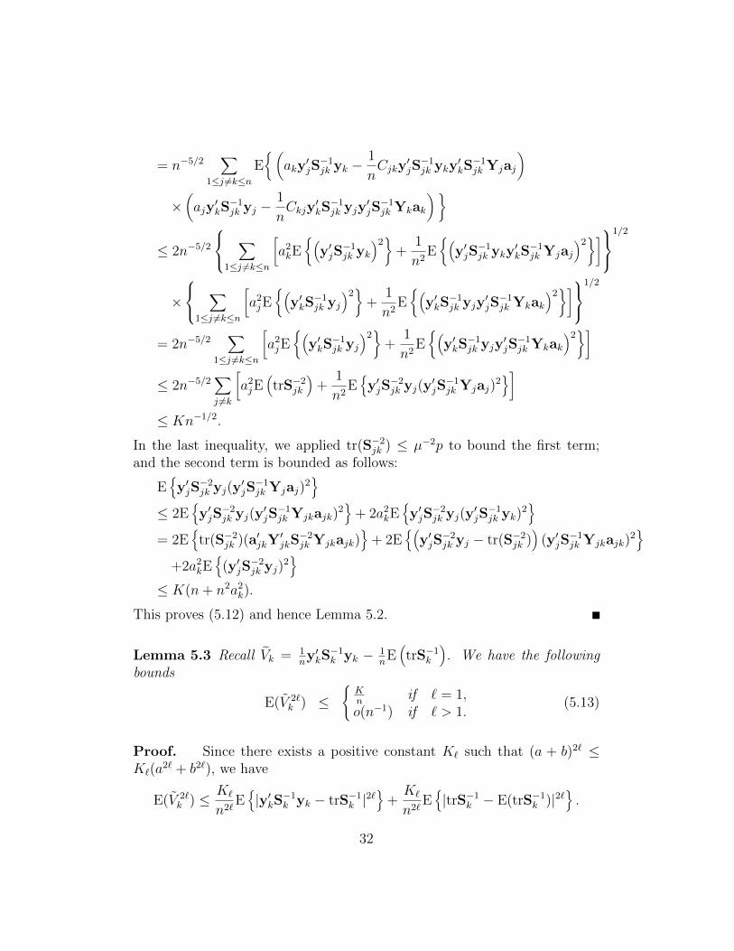
This proves (5.12) and hence Lemma 5.2.

Lemma 5.3 Recall Vk = 1ny′kS

−1k yk − 1

nE(trS−1k

). We have the following

bounds

E(V 2`k ) ≤

{Kn

if ` = 1,o(n−1) if ` > 1.

(5.13)

Proof. Since there exists a positive constant K` such that (a + b)2` ≤K`(a

2` + b2`), we have

E(V 2`k ) ≤ K`

n2`E{|y′kS−1k yk − trS−1k |2`

}+K`

n2`E{|trS−1k − E(trS−1k )|2`

}.

32

To bound the first term, we apply Lemma 9.1 of Bai and Silverstein (2010).To bound the second term, we apply z = iv for v = an−1/2, vy = 1−

√c+√v

with a > 1 in Lemmas 8.20 and 8.21 in Bai and Silverstein (2010).

Acknowledgements

The first author is partially supported by NSFChina 11571067 and PCSIRT;the second author by the Singapore Ministry of Education Academic Re-search Fund R-155-000-141-112; and the third author by the Ministry of Ed-ucation, Science, Sports, and Culture, a Grant-in-Aid for Scientific Research(C), #25330038, 2013-2015.

References

[1] Anderson, T. W. (1951). The asymptotic distribution of certain character-istic roots and vectors. Proc. 2nd Berkeley Symp. on Math. Statist. and Prob.,103–130.

[2] Anderson, T.W. (2003). Introduction to Multivariate Statistical Analysis,3rd ed. Wiley, Hoboken, New Jersey.

[3] Amemiya, Y. (1990). A note on the limiting distribution of certain charac-teristic roots. Statist. & Probab. Lett., 9(5), 465–470.

[4] Bai, Z.D. (1985). A note on the limiting distribution of the eigenvalues of akind of random matrices. J. Math. Research and Exposition, 5(2), 113–118.

[5] Bai, Z.D., Jiang, D., Yao, J.F. and Zheng, S. (2009). Corrections to LRTon large-dimensioanl covariance matrix by RMT. Ann. Statist., 37, 3822–3840.

[6] Bai, Z.D., Liu, H.X. and Wong, W.K. (2011). Asymptotic properties ofeigenmatrices of a large sample covariance matrix. Ann. Appl. Probab., 21,1994–2015.

[7] Bai, Z.D. and Saranadasa, H. (1996). Effect of high dimension: by anexample of a two sample problem. Statistica Sinica, 6, 311–329

33

[8] Bai, Z.D. and Silverstein, J.W. (2004). CLT for linear spectral statisticsof large-dimensional sample covariance matrices. Ann. Probab., 32, 535–605.

[9] Bai, Z.D. and Silverstein, J.W. (2009). Spectral Analysis of Large Dimen-sional Random Matrices, 2nd ed.. Springer.

[10] Fujikoshi, Y. (1977). Asymptotic expansions for the distributions of the la-tent roots in MANOVA and the canonical correlations. J. Multivariate Anal.,7, 386–396.

[11] Fujikoshi, Y. (2015). High-dimensional asymptotic distributions of charac-teristic roots in multivariate linear model MANOVA and canonical correla-tions. In preparation.

[12] Fujikoshi, Y., Himeno, T. and Wakaki, H. (2008). Asymptotic results incanonical discriminant analysis when the dimension is large compared to thesample. J. Statist. Plann. Inference, 138, 3457–3466.

[13] Fujikoshi, Y. and Sakurai, T. (2009). High-dimensional asymptotic ex-pansions for the distributions of canonical correlations. J. Multivariate Anal.,100, 231–241.

[14] Fujikoshi, Y., Ulyanov, V. and Shimizu, R. (2010). Multivariate Analysis:High-Dimensional and Large-Sample Approximations. Wiley, Hoboken, NewJersey.

[15] Glynn, W. J. (1980). Asymptotic representations of the densities of canonicalcorrelations and latent roots in MANOVA when the population parametershave arbitrary multiplicities. Ann. Statist., 8, 468–477.

[16] Hall, P. and Heyde, C.C. (1980). Martingale Limit Theory and its Appli-cations. Academic Press, New York.

[17] Hsu, P. L. (1941). On the limiting distribution of roots of a determinantalequation. J. London Math. Soc., 16, 183–194.

[18] Johnstone, I. M. (2008). Multivariate analysis and Jacobi ensembles: largesteigenvalue, Tracy-Widom limits and rate of convergence. Ann. Statist., 36,2638–2716.

[19] Muirhead, R. J. (1978), Latent roots and matrix variates. Ann. Statist., 6,5–33.

[20] Muirhead, R. J. (1982), Aspect of Multivariate Statistical Theory, Wiley,New York.

34

[21] Muirhead, R. J. and Watermaux, C.M. (1980). Asymptotic distributionsin canonical correlation analysis and other multivariate nonnormal popula-tions. Biometrika, 67, 31–43.

[22] Rosenthal, H. P. (1970). On the subspaces of Lp (p > 2) spanned bysequences of independent random variables. Israel J. Math., 8, 273–303.

[23] Seo, T., Kanda, T. and Fujikoshi, Y. (1994). Asymptotic distributions ofthe sample roots in MANOVA models under nonnormality. J. Japan Statist.Soc., 24, 133-140.

[24] Sugiura, N. (1976). Asymptotic expansions of the distributions of the la-tent roots and latent vectors of the Wishart and multivariate F matrices. J.Multivariate Anal., 6, 500–525.

[25] Wakaki, H., Fujikoshi, Y. and Ulyanov, V. (2014). Asymptotic expan-sions of the distributions of MANOVA test statistics when the dimension islarge. Hiroshima Math. J., 44, 247–259..

[26] Zheng, S. (2012). Central limit theorems for linear spectral statistics oflarge-dimensional F-matrices. Ann. l’Institut Henri Poincaree-Probabilites etStatistiques, 47, 444–476.

35