zenvisage: Effortless Visual Data Exploration

Tarique Siddiqui1 Albert Kim2 John Lee1 Karrie Karahalios1 Aditya Parameswaran1

1University of Illinois (UIUC) 2MIT{tsiddiq2,lee98,kkarahal,adityagp}@illinois.edu alkim@csail.mit.edu

ABSTRACTData visualization is by far the most commonly used mechanism toexplore data, especially by novice data analysts and data scientists.And yet, current visual analytics tools are rather limited in theirability to guide data scientists to interesting or desired visualiza-tions: the process of visual data exploration remains cumbersomeand time-consuming. We propose zenvisage, a platform for effort-lessly visualizing interesting patterns, trends, or insights from largedatasets. We describe zenvisage’s general purpose visual querylanguage, ZQL ("zee-quel") for specifying the desired visual trend,pattern, or insight — ZQL draws from use-cases in a variety of do-mains, including biology, mechanical engineering, commerce, andserver monitoring. While analysts are free to use ZQL directly, wealso expose ZQL via a visual specification interface, which we alsodescribe in this paper. We then describe our architecture and op-timizations, preliminary experiments in supporting and optimizingfor ZQL queries in our initial zenvisage prototype, as well as a userstudy to evaluate whether data scientists are able to effectively usezenvisage for real applications.

1. INTRODUCTIONThe rising popularity of visual analytics tools have paved the

way for the democratization of data exploration and data science.Increasingly, amateur data scientists from a variety of domains andsectors now have the ability to analyze and derive insights fromdatasets of increasing size and complexity. The standard recipefor data science then goes as follows: the data scientist loads thedataset into a visual analytics tool like Tableau [4] or Spotfire [3],or even a domain-specific data exploration tool, they create or se-lect visualizations, and then examine whether those visualizationscapture desired patterns or insights. If these visualizations do notmeet the desired requirements, the process is repeated by examin-ing a whole range of additional visualizations until they find thevisualizations that do. This data exploration process is often cum-bersome and time-consuming, since the number of visualizationsthat the data scientists need to examine to derive desired insightsgrows rapidly with size of the dataset: the number of records aswell as the number of attributes across different relations. To illus-trate, consider the following real case studies that demonstrate thelimitations of current data exploration tools.Case Study 1: Advertising Analytics. Advertisers—from smallbusinesses to large corporations—at search company Google areoften interested in examining their portfolio of sponsored searchand display ads in order to see if their advertising campaigns areperforming as expected. For instance, an advertiser may be inter-ested in seeing if there are any keywords that are behaving unusu-ally with respect to other keywords in the Asia-Pacific region. Todo this using the current visual analytics tools available at Google,

the advertiser needs to generate the plot of click-through rates (CTR)over time for each keyword, and then examine each one of them inturn.Case Study 2: Genomic Data Analysis. Clinical researchers atNIH’s BD2K (Big Data 2 Knowledge) Center at the University ofIllinois are interested to quickly gain insights about gene-gene andprotein-protein relationships in the context of various clinical tri-als. For instance, one common task that the clinical researcherswould like to perform is to compare two classes of genes and seewhat factors help them visually understand the differences betweenthese classes. (For example, one class could be those genes pos-itively correlated with cancer, while the rest are not.) To do thisusing the current visual analytics tools available at the center, theseresearchers would have to generate scatterplots corresponding toall pairs of factors, and examine each one in turn to see if the twoclasses of genes are well-separated in these scatterplots.Case Study 3: Engineering Data Analysis. Battery scientists atCarnegie Mellon University are interested in performing visual ex-ploration of a dataset containing electrolytes and their propertiesat various scales—molecular, meso, and continuum scales. For in-stance, one task that scientists often do is find classes of solventsthat have desired behavior: for instance, solvents whose solvationenergy of Li+ vs. vs the boiling point is an increasing trend. Todo this using current tools, these scientists would need to generatethese plots for all solvent classes and manually examine each one.Case Study 4: Server Monitoring Analysis. The server monitor-ing team at company Facebook has noticed a spike in the per-queryresponse time for Image Search in Russia around August 15, afterwhich the response time has flattened out. The team would like toidentify if there are other attributes that have a similar behaviorwith per-query response time, which may indicate the reason forthe spike and subsequent flattening. To do this, the server moni-toring team needs to generate visualizations for different metrics asa function of the date, and see if any of them has similar behaviorto the response time for Image Search. Given that the number ofmetrics is likely in the thousands, this could take a very long time.Case Study 5: Mobile App Analysis. The complaints team at themobile platform team of company Google have noticed that a cer-tain mobile app has received many complaints. They would like tofigure out what is different about this app relative to others. To dothis, they would need to plot various metrics for this app to figureout why it is behaving anomalously. For instance, they may lookat network traffic generated by this app over time, or at the distri-bution of energy consumption across different users. In all of thesecases, the team would need to generate several visualizations man-ually and browse through all of them in the hope of finding whatcould be the issues with the app.

In all of the above scenarios, there is the following recurring theme:

1

arX

iv:1

604.

0358

3v1

[cs

.DB

] 1

2 A

pr 2

016

generate a large number of visualizations and evaluate each one fora desired visual property.

Instead, our goal in this paper is to build zenvisage, a visualanalytics system that can “fast-forward” to the desired insights,thereby minimizing significant burden on the part of the data scien-tists or analysts in scenarios like the ones described above.

Given the wealth of data analytics tools available, one may askwhy a new tool is needed. With these tools, selecting the “right”view on the data that reveals the “desired” insight still remains la-borious and time-consuming. The onus is on the user to manuallyspecify the view they want to see, and then repeat this until theyget the desired view. In particular, existing tools are inadequate,including: 1) Relational databases: Databases are powerful andefficient, but the rigidity of the syntax limits the users ability toexpress queries like “show me visualizations of keywords whereCTR over time in Asia is behaving unusually”. That said, our so-lution is an abstraction that sits atop traditional relational databasesas a storage and computation engine. 2) Data mining tools: Datamining tools are hard to expect users to use, since it involves ex-tensive programming, as well as an understanding of which datamining tool applies to what purpose. Certainly, expressing eachquery will require extensive programming and manual optimiza-tion (not desirable for ad-hoc querying). 3) Visual analytics tools:Visual analytics tools like Tableau and Spotfire have made it mucheasier for business analysts to analyze data; that said, the user needsto exactly specify what they want to visualize. If the visualizationdoes not yield the desired insight, then the user must try again, nowwith a different visualization. One can view zenvisage as a gener-alization of standard visualization specification tools like Tableau;capturing all the Tableau functionality, while providing the meansto skip ahead to the desired insights. We describe related work inmore detail in Section 7.

In this paper, we describe the specification for our query lan-guage for zenvisage, ZQL. We describe how ZQL is powerful enoughto capture the use cases described above as well as many manyother use cases (Section 2). Our primary contribution in this paperis ZQL, which resulted from a synthesis of desiderata after dis-cussing with analytics teams from a variety of domains (describedabove). We develop a number of simple optimizations that we canuse to simplify the execution of ZQL queries by minimizing thenumber of SQL queries that are issued (Section 3). We also de-scribe our initial prototype of zenvisage which implements a subsetof ZQL, the end-user interface, as well as the underlying systemsarchitecture (Section 4). We describe our initial performance exper-iments (Section 5). We present a user study focused on evaluatingthe effectiveness and usability of zenvisage (Section 6). In the ap-pendix, we present additional details of our query language, withcomplete examples (Appendix C) and describe the capabilities ofour language in some detail (Appendix D).

2. QUERY LANGUAGEOur system zenvisage’s query language, ZQL, provides users a

flexible and intuitive mechanism to specify desired insights fromvisualizations. The user may either directly write ZQL queries,or they may use the zenvisage front-end, which transforms all re-quests to ZQL queries internally. Our design of ZQL builds onwork on visualization specification for visual analytics tools andplatforms, in particular from Polaris [44], and Grammar of Graph-ics [50]. Indeed, zenvisage is intended to be a generalization ofPolaris/Tableau [44], and hence must encompass Polaris function-ality as well as additional functionality for searching for desiredtrends, patterns, and insights. In addition, ZQL also draws heavyinspiration from the Query by Example (QBE) Language [52] and

uses a similar a similar table-based interface. (Notice, however,that ZQL is not tied to this interface, as we describe in Section 2.1,and can be used in other ways.)

Our goal for ZQL was to ensure that users would be able to ef-fortlessly express complex requirements using a small number ofZQL lines. Furthermore, the language itself should be robust andgeneral enough to capture the wide range of possible visual queries.As we will see later, despite the generality of the language, we havebuilt an automatic parser and optimizer that can apply to any ZQLquery and transforms it into a collection of SQL queries, along withpost-processing that is run on the results of the SQL queries: thismeans that zenvisage can use as a backend any traditional rela-tional database. To illustrate the power and the generality of thelanguage, we now illustrate a few examples of ZQL queries, beforewe dive into the ZQL formalism. To make it easy to follow withoutmuch background, we use a fictitious product sales-based datasetthroughout this paper in our query examples—we will reveal at-tributes of this dataset as we go along.

Due to space limitations, we are unable to describe the full capa-bilities and limitations of ZQL here; these details can be found inAppendix D, with additional complete examples in Appendix C.Query 1: Depict a collection of visualizations. Table 1 depicts avery simple ZQL query. This ZQL query retrieves the data for eachproduct’s total sales over years bar chart visualization for productssold in the US. As the reader can probably guess, the ‘year’ and‘sales’ in the X and Y columns dictate the x- and y- axes of thevisualizations, and the location=‘US’ in the Constraints columnconstrains the data to items sold in the US. Then, for the Z col-umn, we use the variable v1 to iterate over ‘product’.*, the setof all possible product values. The bar.(y=agg(‘sum’)) denotesthat the visualization is a bar chart where the y-values are aggre-gated using the SUM function grouped by both the x- and z- axes.The Process column is typically used to filter, sort, or compare vi-sualizations, but in this case, since we want the full set of visual-izations (one for every product), we leave the the Process columnblank. This generates a separate sales vs. year plot for each prod-uct, giving a collection of resulting visualizations. This collectionof visualizations is referred to using the variable f1, with the * in-dicating that these visualizations are to be output to the user. (Notethat both variables v1 and f1 are redundant in this current query,but will come in handy for other more complex queries.) Naturally,if the number of products is large, this query could lead to a largenumber of visualizations being displayed, and so may not be desir-able for the user to peruse. Later, we will describe mechanisms toconstrain the space of visualizations that are displayed to be thosethat satisfy a user need. The idea that we can represent a set ofvisualizations with just one line is a powerful one, and it is part ofwhat makes ZQL such an expressive language.Query 2: Find the product which has the most similar sales trendas the user-drawn input trend line. Table 2 provides an examplewhich integrates ZQL with user-drawn trend lines. Using zenvis-age’s front-end, the user can draw a trend line1, which ZQL canuse as an input and compare against other visualizations from thedatabase. In Table 2, we use - in the -f1 to denote that it correspondsto a visualization provided by the user. After the user input line, wesee a second line which looks similar to the example in the firstquery; f2 iterates over the set of sales over year visualizations foreach product. With the Process column, we can compare the visu-alizations f1 and f2 with some distance metric D for every productvalue in v1. argmin looks through the comparisons and selects the

1zenvisage provides many options for user input, including directly drawing a visu-alization using the zenvisage front-end, providing a set of data values, or specifyinga list of constraints that the visualization must satisfy.

2

Name X Y Z Constraints Viz Process*f1 ‘year’ ‘sales’ v1 <– ‘product’.* location=‘US’ bar.(y=agg(‘sum’))

Table 1: A ZQL query which returns the set of total sales over years bar charts for each product sold in the US.Name X Y Z Process

-f1f2 ‘year’ ‘sales’ v1 <– ‘product’.* v2 <– argminv1[k = 1]D( f 1, f 2)

*f3 ‘year’ ‘sales’ v2Table 2: A ZQL query which returns the product which has the most similar sales over year visualization as the given user-drawn trend line.

Name X Y Z Constraints Processf1 ‘year’ ‘sales’ v1 <– ‘product’.* location=‘US’ v2 <– arganyv1[t > 0]T ( f 1)f2 ‘year’ ‘sales’ v1 location=‘UK’ v3 <– arganyv1[t < 0]T ( f 2)f3 ‘year’ ‘sales’ v4 <– (v2.range & v3.range) v5 <– R(10,v4, f 3)

*f4 ‘year’ ‘profit’ v5Table 3: A ZQL query which returns the profit over years visualizations for products that have positive sales over years trends for the US buthave negative sales over years trends for the UK.

one product which minimizes the distance. Finally, f3 outputs thesales over year visualization for that product. Thus, with Table 2,we have managed to perform a similarity search for visualizationsagainst a user-drawn input.Query 3: Find and visualize profit for products that are doing wellon sales in the US but badly in the UK. Finally, we look at an evenmore complex example in Table 3. This query captures the scenarioof wishing to find the profit over years visualizations for productsthat have positive sales over years trends for the US but have nega-tive sales over years trends for the UK. This is a visual query manybusiness users would like to be able to perform. However, the wayusers would currently achieve this is by manually visualizing thesales over years for both the US and the UK for every item and re-membering which item had the most discrepancy. With ZQL, thevisual query can be expressed with three lines. Line one retrievesthe set of sales over years visualizations for each product sold inthe US and filters it to only include the ones in which the over-all trend (T ( f 1)) is positive (t > 0). Likewise, the the second lineretrieves the type of visualizations for products sold in the UK andfilters it to only include the ones with negative (t < 0) overall trends(T ( f 2)). The third row combines the results of the two by takingthe intersection of the sets of products (v2.range & v3.range)and labels the profit over years visualizations for these products asf3. Then 10 visualizations which form the representative set of thevisualizations in f3 are chosen using the function R, and returned.

In the rest of this section, we go more in depth into the ZQLlanguage and provide a formal specification. Additional real-worldexamples of how ZQL can be used can be found in Appendix C.

2.1 FormalizationWe now formally describe the ZQL syntax. Throughout, we as-

sume that we are operating on a single relation or a star schemawhere the attributes are uniquely defined (barring key-foreign keyjoins). In general, ZQL could be applied to arbitrary collectionsof relations by letting the user precede an attribute A with the rela-tion name R, e.g., R.A. But for ease of exposition, we focus on thesingle relation case.

2.1.1 OverviewAs described earlier, a ZQL query is composed using a table,

much like a QBE query. Unlike QBE, the columns of a ZQL querydo not refer to attributes of the table being operated on; instead,they are predefined, and have fixed semantic meanings. In particu-lar, at a high level, the columns are: (i) Name: providing an iden-tifier for a set or collection of visualizations, and allowing us toindicate if a specific set of visualizations are to be output (ii) X, Y:specifying the X and Y axes of the collections of visualizations, re-stricted to sets of attributes (iii) Z (optional): specifying the “slice”(or subset) of data that we’re varying restricted to sets of attributesalong with values for those attributes; (iv) Constraints (optional):

specifying optional constraints applied to the data prior to any vi-sualizations or collections of visualizations being generated (v) Viz(optional): specifying the mechanism of visualization, e.g., a barchart, scatterplot, as well as the associated transformation, or ag-gregation, e.g., the X axis is binned in groups of 20, while theY axis attribute is aggregated using SUM. If this is not specified,standard rules of thumb are used to determine the appropriate vi-sualization [51, 32]. (vi) Process (optional): specifying the “op-timization” operation performed on a collection of visualizations,typically intended towards identifying desired visualizations.

A ZQL query may have any number of rows, and conceptuallyeach row represents a set of visualizations of interest. The usercan then process and filtrate these rows until she is left with onlythe output visualizations she is interested in. The result of a ZQLquery is the data used to generate visualizations. The zenvisagefront-end then generates the visualizations for the user to peruse.

An astute reader may wonder why we chose a table as an in-terface for entering ZQL queries. Our choice has to do with ourend-users: primarily non-programmers who are used to drop-downmenus and spreadsheet tools like Microsoft Excel, who would feelmuch more at home with a tabular interface. Specifically, the tabu-lar skeleton ensures that users would not “miss out” on key columns,and can view the query on the web-client front-end as a collectionof steps, each of which corresponds to a row, and ensure correctsyntax. Indeed, our user study validates this point — even userswith minimal programming experience can still use ZQL profi-ciently after a short tutorial. Additionally, this interface is muchmore suited for embedding into an interactive web-client. Thatsaid, a user with more experience in programming may find theinterface restrictive, and may prefer issuing the query as a functioncall within a programming language. Nothing in our underlyingZQL backend is tied to the tabular interface: specifically, we al-ready support the issuing of ZQL queries within our Java clientlibrary: users can easily embed ZQL queries into other computa-tion. In the future, we plan to write wrappers for other libraries sothat users can embed ZQL into computation in other settings. Weare exploring the use of Apache Thrift [43] for this purpose.

2.1.2 X and Y ColumnsAs mentioned, each row can be thought of as a set of visualiza-

tions, and the X and Y columns represent the x- and y- axes forthose visualizations. In Table 1, the first row’s visualizations willhave ‘year’ as their x-axis and ‘profit’ as their y-axis.

The only permissible entries for the X or Y column are eithera single attribute from the table, or a set of attributes, with a vari-able to iterate over them. The exact semantics of variables andsets are discussed later in Section 2.1.7, but essentially, a columnis allowed to take on any attribute from the set. For example, inTable 4, the y-axis is allowed to take on either ‘profit’ or ‘sales’ asits attribute. Because the y-axis value can be taken from a set of

3

attributes, the resulting output of this query is actually the set ofvisualizations whose x-axis is the ‘time’ and the y-axis is one of‘profit’ and ‘sales’ for the ‘stapler’. This becomes a powerful no-tion later in the process column where we try to iterate over a setof visualizations and identify desired ones to return to the user orselect for down-stream processing.

Name X Y Constraints*f1 ‘year’ y1 <– {‘profit’, ‘sales’} product=‘stapler’

Table 4: A query for a set of visualizations, one of which plots profitover year and one of which plots sales over time for the stapler.

2.1.3 Z ColumnThe Z column is used to either focus our attention on a specific

slice (or subset) of the dataset or iterate over a set of slices for oneor more attributes. To specify a set of slices, the Z column mustspecify (a) one or more attributes, just like the X and Y column,and (b) one or more attribute values for each of those attributes —which allows us to slice the data in some way. For both (a) and(b) the Z column could specify a single entry, or a variable asso-ciated with a set of entries. Table 5 gives an example of using theZ column to visualize the sales over time data specifically with re-gards to the ‘chair’ and ‘desk’ products, one per line. Note that theattribute name and the attribute value are separated using a period.

Table 6 depicts an example where we iterate over a set of slices(attribute values) for a given attribute. This query returns the setof sales over time visualizations for each product. Here, v1 bindsto the values of the ‘product’ category. Since ZQL internally as-sociates attribute values with their respective attributes, there is noneed to specify the attribute explicitly for v1. Another way to thinkabout this is to think of v1 <– ‘product’.* as syntactic sugar for‘product’.v1 <– ‘product’.*. The * symbol denotes all possiblevalues; in this case, all possible values of the ‘product’ attribute.

Name X Y Z*f1 ‘year’ ‘sales’ ‘product’.‘chair’*f2 ‘year’ ‘sales’ ‘product’.‘desk’

Table 5: A ZQL query for a set of visualizations which returnsthe sales over year visualization for chairs and the sales over timevisualization for desks.

Name X Y Z*f1 ‘year’ ‘sales’ v1 <– ‘product’.*

Table 6: A ZQL query for a set of visualizations which returns theset of sales over year visualizations for each product.

Furthermore, the Z column can be left blank if the user does notwish to slice the data in any way.

2.1.4 Constraints ColumnThe constraints column is used to specify further constraints on

the set of data used to generate the set of visualizations. Concep-tually, we can view the constraints column as being applied to thedataset first, following which a collection of visualizations are gen-erated on the constrained dataset.

While the constraints column may appear to overlap in function-ality with the Z column, the constraints column does not admit it-eration via variables in the way the Z, X or Y column, admits. Itis instead intended to apply a fixed boolean predicate to each tu-ple of the dataset prior to visualization in much the same way theWHERE clause is applied in SQL. (We discuss this issue furtherin Section 2.1.7.) A blank constraints column means no additionalconstraints are applied to the data prior to visualization.

2.1.5 Viz ColumnGiven the data from the X, Y, Z, and Constraints columns, the

Viz column determines how the data is shaped or modified beforereturning it as a visualization to the user. There are two aspects to

the Viz column: first, the visualization type (e.g., bar chart, scat-ter plot), and the summarization type (e.g., binning or grouping insome way, aggregating in some way). These two aspects are akin tothe geometric and statistical transformation layers from the Gram-mar of Graphics, a language for specifying visualizations, and theinspiration behind ggplot [48].

In ZQL, the Viz column specifies the visualization type and thesummarization using a period delimiter. Functions are used to rep-resent both the visualization type and the summarization. Con-sider the query in Table 7. Here, the user specifies that she wantsa bar chart, with bar, and specifies the type of summarization inthe accompanying tuple: x=bin(20) denotes that x-axis should bebinned into bins of size 20, and y=agg(‘sum’) runs the SUM ag-gregation on the y-values when grouped by both the bins of thex-axis and the values in the z-axis, (if any are specified).

Although we can explicitly specify the Viz column, often we canleave the Viz column blank. In such cases, we would apply well-known rules of thumb for what types of visualization and summa-rization would be appropriate given specific X and Y axes. Workon recommending appropriate visualization types dates back to the80s [32], that both Polaris/Tableau [44], and recent work buildson [51, 25], determining the best visualization type by examiningthe schema and statistical properties. In many of our examples ofZQL queries, we omit the Viz column for this reason.

2.1.6 Name ColumnFor any row of a ZQL query, the combination of X, Y, Z, Con-

straints, and Viz columns together represent the visual componentof that row. A visual component represents a set of visualizations.The Name column allows us to provide a name to this visual com-ponent by binding a variable to it. These variables can be used inthe Process column to subselect the desired visualizations from theset of visualizations, as we will see subsequently.

In the ZQL query given by Table 8, we see that the names forthe visual components of the rows are named f1, f2, and f3 in orderof the rows. For the first row, the visual component is a singlevisualization, since there are no sets, and f1 binds to the singlevisualization. For the second row, we see that the visual componentis over the set of visualizations with varying Z column values, andf2 binds to the variable which iterates over this set. Note that f1 andf3 in Table 8 are prefaced by a * symbol. This symbol indicatesthat the visual component of the row is designated to be part of theoutput. As can be seen in the example, multiple rows can be partof the output, and in fact, even a row could correspond to multiplevisualizations. Visualizations corresponding to all the rows markedwith * are processed by the zenvisage frontend, which displayseach of them.

2.1.7 Sets and VariablesBefore we move on to the Process column, we must give the

full formal semantics for sets and variables in ZQL. As we havealluded many times, sets in ZQL must always be accompanied bya variable which iterates over that set. This requirement was madeto ensure that ZQL traverses over sets of visualizations in a con-sistent order when making comparisons. Consider Table 10, whichshows a query that iterates over the set of products, and for eachof these products, compares the sales over years visualization withthe profits over years visualization. Without a variable enforcing aconsistent iteration order over the set of products, it is possible thatthe set of visualizations could be traversed in unintended ways. Forexample, the sales vs. year plot for chairs from the first set could becompared with the profit vs. year plot for desks in the second set,which is not what the user intended. By reusing v1 in both the first

4

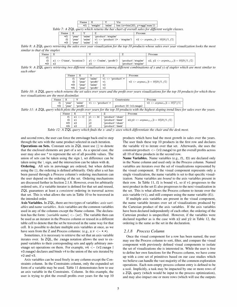
Name X Y Viz*f1 ‘weight’ ‘sales’ bar.(x=bin(20), y=agg(‘sum’))

Table 7: A ZQL query which returns the bar chart of overall sales for different weight classes.Name X Y Z Process

*f1 ‘year’ ‘sales’ ‘product’.‘stapler’f2 ‘year’ ‘sales’ v1 <– ‘product’.(* - ‘stapler’) v2 <– argminv1[k = 10]D( f 1, f 2)

*f3 ‘year’ ‘sales’ v2Table 8: A ZQL query retrieving the sales over year visualization for the top 10 products whose sales over year visualization looks the mostsimilar to that of the stapler.

Name X Y Z Process-f1f2 x1 <– {‘time’, ‘location’} y1 <– {‘sales’, ‘profit’} ‘product’.‘stapler’ x2, y2 <– argminx1,y1[k = 10]D( f 1, f 2)

*f3 x2 y2 ‘product’.‘stapler’Table 9: A ZQL query retrieving two different visualisations (among different combinations of x and y) of stapler which are most similar toeach other

Name X Y Z Processf1 ‘year’ ‘sales’ v1 <– ‘product’.*f2 ‘year’ ‘profit’ v1 v2 <– argmaxv1[k = 10]D( f 1, f 2)

*f3 ‘year’ ‘sales’ v2*f4 ‘year’ ‘profit’ v2

Table 10: A ZQL query which returns the set sales over years and the profit over years visualizations for the top 10 products for which thesetwo visualizations are the most dissimilar.

Name X Y Z Constraints Processf1 ‘year’ ‘sales’ v1 <– ‘product’.* v2 <– argmaxv1[k = 10]T ( f 1)

*f2 ‘year’ ‘profit’ product IN (v2.range)Table 11: A ZQL query which plots the profit over years for the top 10 products with the highest sloping trend lines for sales over the years.

Name X Y Z Processf1 x1 <– C y1 <– M ‘product’.‘chair’f2 x1 y1 ‘product’.‘desk’ x2,y2 <– argmaxx1,y1[k = 10]D( f 1, f 2)

*f3 x2 y2 ‘product’.‘chair’*f4 x2 y2 ‘product’.‘desk’

Table 12: A ZQL query which finds the x- and y- axes which differentiate the chair and the desk most.

and second rows, the user can force the zenvisage back-end to stepthrough the sets with the same product selected in each iteration.Operations on Sets. Constant sets in ZQL must use {} to denotethat the enclosed elements are part of a set. As a special case, theuser may also use * to represent the set of all possible values. Theunion of sets can be taken using the sign |, set difference can betaken using the \ sign, and the intersection can be taken with &.Ordering. All sets in zenvisage are ordered, but when definedusing the {}, the ordering is defined arbitrarily. Only after a set hasbeen passed through a Process column’s ordering mechanism canthe user depend on the ordering of the set. Ordering mechanismsare discussed further in Section 2.1.8. However, even for arbitrarilyordered sets, if a variable iterator is defined for that set and reused,ZQL guarantees at least a consistent ordering in traversal acrossthat set. This is what allows the sets in Table 10 to be traversed inthe intended order.Axis Variables. In ZQL, there are two types of variables: axis vari-ables and name variables. Axis variables are the common variablesused in any of the columns except the Name column. The declara-tion has the form: 〈variable name〉 <– 〈set〉. The variable then canbe used as an iterator in the Process column or reused in a differenttable cell to denote that the set be traversed in the same way for thatcell. It is possible to declare multiple axis variables at once, as wehave seen from the Z and Process columns: (e.g., z.v <– *.*).

Sometimes, it is necessary to retrieve the set that an axis variableiterates over. In ZQL, the .range notation allows the user to ex-pand variables to their corresponding sets and apply arbitrary zen-visage set operations on them. For example, v4 <– (v2.range |v3.range) declares and binds v4 to the union of the sets iterated byv2 and v3.

Axis variables can be used freely in any column except the Con-straints column. In the Constraints column, only the expanded setform of a variable may be used. Table 11 demonstrates how to usean axis variable in the Constraints. Column. In this example, theuser is trying to plot the overall profits over years for the top 10

products which have had the most growth in sales over the years.The user finds these top 10 products in the first row and declaresthe variable v2 to iterate over that set. Afterwards, she uses theconstraint product <– (v2.range) to get the overall profits acrossall 10 of these products in the second row.Name Variables. Name variables (e.g., f1, f2) are declared onlyin the Name column and used only in the Process column. Namedvariables are iterators over the set of visualizations represented bythe visual component. If the visual component represents only asingle visualization, the name variable is set to that specific visual-ization. Name variables are bound to the axis variables present intheir row. In Table 11, f1 is bound v1, so if v1 progresses to thenext product in the set f1 also progresses to the next visualization inthe set. This is what allows the Process column to iterate over theaxis variable (v1), and still compare using the name variable (f1).

If multiple axis variables are present in the visual component,the name variable iterates over set of visualizations produced bythe Cartesian product of the axis variables. If the axis variableshave been declared independently of each other, the ordering of theCartesian product is unspecified. However, if the variables weredeclared together as is the case with x2 and y2 in Table 12, theordering is the same as the set in the declaration.

2.1.8 Process ColumnOnce the visual component for a row has been named, the user

may use the Process column to sort, filter, and compare the visualcomponent with previously defined visual components to isolatethe set of visualizations she is interested in. While the user is freeto define her own functions for the Process column, we have comeup with a core set of primitives based on our case studies whichwe believe can handle the vast majority of the common explorationoperations. Each non-empty process column entry is defined to bea task. Implicitly, a task may be impacted by one or more rows ofa ZQL query (which would be input to the process optimization),and may also impact one or more rows (which will use the outputs

5

Name X Y Z Processf1 ‘year’ ‘sales’ v1 <– ‘product’.* v2 <– R(10,v1, f 1)f2 ‘year’ ‘sales’ v2 v3 <– argmaxv1[k = 10] minv2D( f 1, f 2)

*f3 ‘year’ ‘sales’ v3Table 13: A ZQL query which returns 10 sales over years visualizations for products which are outliers compared to the rest.

of the process optimization), as we will see below.Functional Primitives. First, we introduce three simple functionsthat can be applied to visualizations: T , D, and R. zenvisage willuse default settings for each of these functions, but the user is freeto specify their own variants for each of these functions that aremore suited to their application.• T ( f ) measures the overall trend of visualization f . It is positive ifthe overall trend indicates “growth” and negative if the overall trendgoes “down”. There are obviously many ways that such a functioncan be implemented, but one example implementation might be tomeasure the slope of a linear fit to the given input visualization f .• D( f , f ′) measures the distance between the two visualizations fand f ′. For example, this might mean calculating the Earth Mover’sDistance or the Kullback-Leibler Divergence [49] between the in-duced probability distributions.• R(k,v, f ) computes the set of k-representative visualizations givenan axis variable, v, and an iterator over the set of visualizations, f .Different users might have different notions of what representativemeans, but one example would be to run k-means clustering on thegiven set of visualizations and return the k centroids. In additionto taking in a single axis variable, v, R may also take in a tuple ofaxis variables to iterate over. The return value of R is the set of axisvariable values which produced the representative visualizations.Optimization. Given these functional primitives, ZQL also pro-vides some default sorting and filtering mechanisms: argmin, argmax,and argany. Although argmin and argmax are usually used to findthe best value for which the objective function is optimized, ZQLtypically returns the top-k values, sorted in order. argany is used toreturn any k values. In addition to the top-k, the user might also liketo specify that she wants every value for which a certain thresholdis met, and ZQL is able to support this as well. Specifically, the ex-pression v2 <– argmaxv1[k = 10]D( f 1, f 2) returns the top 10 v1values for which D( f 1, f 2) are maximized, sorts those in decreas-ing order of the distance, and declares the variable v2 to iterate overthat set. This could be useful, for instance, to find the 10 visualiza-tions with the most variation on some attributes. The expressionv2 <– argminv1[t < 0]D( f 1, f 2) returns the v1 values for whichthe objective function D( f 1, f 2) is below the threshold 0, sorts thevalues in increasing order of the objective function, and declaresv2 to iterate over that set. If a filtering option (k,t) is not specified,the mechanism simply sorts the values, so v2 <– argminv1T ( f 1)would bind v2 to iterate over the values of v1 sorted in increas-ing order of T ( f 1). v2 <– arganyv1[t > 0]T ( f 1) would set v2 toiterate over the values of v1 for which the T ( f 1) is greater than 0.

Note that the mechanisms may also take in multiple axis vari-ables, as we saw from Table 12. The mechanism iterates over theCartesian product of its input variables. If a mechanism is given kaxis variables to iterate over, the resulting set of values must also bebound to k declared variables. In the case of Table 12, since therewere two variables to iterate over, x1 and y1, there are two outputvariables, x2 and y2. The order of the variables is important as thevalues of the ith input variable are set to the ith output variable.User Exploration Tasks. By building on these mechanisms, theuser can perform most common tasks. This includes the similari-ty/dissimilarity search performed in Table 10, to find products thatare dissimilar; the comparative search performed in Table 12, toidentify attributes on which two slices of data are dissimilar, or eventhe outlier search query shown in Table 13, to identify the productsthat are outliers on the sales over year visualizations. Note that inTable 13, we use two levels of iteration.

3. QUERY EXECUTIONIn zenvisage, ZQL queries are automatically parsed and exe-

cuted by the zenvisage backend. Assuming the dataset is storedin a database, the ZQL compiler is capable of translating any ZQLquery into a collection of SQL queries and accompanying post-processing computations that must be performed over the resultsof the SQL queries. Next, we first describe how a naive zenvisagecompiler would translate ZQL queries. Then, we provide optimiza-tions over this naive zenvisage compiler to reduce the number ofSQL queries that must be issued. Note that in this section, we omitthe FROM clause: this is implied and always fixed.

3.1 Naive TranslationA ZQL query can be broken up into two parts: the visual compo-

nents and the the Process column. In the ZQL compiler, the visualcomponents determine the set of data zenvisage needs to retrievefrom the database, and the Process column translates into the post-processing computation to be done on the returned data.

zenvisage’s naive ZQL compiler performs the following opera-tions for each row of a ZQL query. For each row, at a high level, theZQL compiler issues a SQL query corresponding to each visualiza-tion in the set of visualizations specified in the visual component.Notice that this approach is akin to what a visual analyst manuallygenerating each visualization of interest and perusing it would do;here, we are ignoring the human perception cost. More formally,for each row (i.e., each name variable), the ZQL compiler loopsover all combinations of values for each of the n axis variables inthe visual component corresponding to that row, and for each com-bination, issues a SQL query, the results of which are stored in thecorresponding location in an n dimensional array. (Essentially, thiscorresponds to a nested for loop n levels deep.) Each generatedSQL query has the form:

SELECT X, YWHERE Z=V and (CONSTRAINTS)ORDER BY X

If the summarization is specified, additional clauses such as GRO-UP BYs and aggregations may be added. The results of each visu-alization are stored in an n-dimensional array at the current index.If n is 0, the name variable points directly to the data.

Once the name variable array has been filled in with results fromthe SQL queries, the ZQL compiler generates the post-processingcode from the task in the Process column. At a high level, ZQLloops through all the visualizations, and applies the objective func-tion on each one. In particular, for each input axis variable in themechanism, a for loop is created and nested. The input axis vari-ables are then used to step through the arrays specified by the namevariable, and the objective function is called at each iteration. In-stances of name variables are updated with the correct index basedon the axis variables it depends on. The functions themselves areconsidered black boxes to the ZQL compiler and are unaltered.

We provide the psuedocode of the compiled version of the queryexpressed in Table 14 in Listing 1 in the appendix.

3.2 OptimizationsWhile the translation process of the naive ZQL compiler is sim-

ple and easy to follow, there is plenty of room for optimization. Inparticular, we look at three levels of optimization which focus onbatching SQL queries. We found that the time it took to submit andwait for SQL queries was a bottleneck, and reducing the overallnumber of SQL queries can reduce performance significantly.

6

Name X Y Z Constraints Viz Processf1 ‘year’ ‘sales’ v1 <– P location=‘US’ bar.(y=agg(’sum’)) v2 <– arganyv1[t > 0]T ( f 1)f2 ‘year’ ‘sales’ v1 location=‘UK’ bar.(y=agg(’sum’)) v3 <– arganyv1[t < 0]T ( f 2)

*f3 ‘year’ ‘profit’ v4 <– (v2.range | v3.range) bar.(y=agg(’sum’))Table 14: A ZQL query which returns the profit over time visualizations for products in user-specified set P that have positive sales over timetrends for the US but have negative sales over time trends for the UK.

Name X Y Z Constraints Viz Processf1 ‘location’ ‘sales’ v1 <– P year=‘2010’ bar.(y=agg(’sum’))f2 ‘location’ ‘sales’ v1 year=‘2015’ bar.(y=agg(’sum’)) v2 <– argmaxv1[k = 10]D( f 1, f 2)

*f3 ‘location’ ‘profit’ v2 year=‘2010’ bar.(y=agg(’sum’))*f4 ‘location’ ‘profit’ v2 year=‘2015’ bar.(y=agg(’sum’))

Table 15: A ZQL query which returns the profit over location visualizations for products in user-specified set P that have the most differentsales over location trends between 2010 and 2015.

While none of these optimizations may seem particularly sur-prising, it required a substantial amount of effort to identify howthese optimizations may be applied automatically to any ZQL query.Our proposed optimizations are reminiscent of multi-query opti-mization techniques [41], but are tailored to ZQL queries.Intra-Line Optimization. The first level of optimization batchesthe SQL queries for a row into one query. For example, we see thatfor the first row Table 14, that a separate query is being made forevery product in Listing 1 in the appendix. Instead, we can retrievethe data for all products in one SQL query:

SELECT year, SUM(sales), productWHERE product IN P and location=‘US’GROUP BY product, yearORDER BY product, year

If the axis variable is in either the X or Y columns, we retrievethe data for the entire set of attributes the axis variable iteratesover. More concretely, if we have axis variable y1 <– {‘sales’,‘profit’}, our SQL query would look like:

SELECT year, SUM(sales), SUM(profit), productWHERE product IN P and location=‘US’GROUP BY product, yearORDER BY product, year

This optimization cuts down the number of queries by the sizes ofsets the axis variables range over, and therefore will lead to sub-stantial performance benefits, as we will see in the experiments.

A side effect of batching queries is that the compiled code mustnow have an extra phase to extract the data for different visualiza-tions from the combined results. However, since the ZQL compilerincludes an ORDER BY clause, the overhead of this phase is min-imal.Intra-Task Optimization. In addition to combining SQL querieswithin a row, SQL queries may also be batched across ZQL rows.However, in general, it may not be possible to compose queriesacross rows into a single SQL query, since different rows may ac-cess completely different attributes. Instead, our optimization isto batch multiple SQL queries from different rows into a single re-quest to the database, effectively pipelining the data retrieval. How-ever, tasks in ZQL frequently filter and limit the space of visualiza-tions being looked at. Moreover, visualizations from subsequentrows may depend on the output values of previous tasks, so it isnot possible to batch queries across tasks. Therefore, we batch intoa single request all SQL queries for task-less rows leading up to arow with a task. In Table 15, this optimization would batch rows 1and 2 together and rows 3 and 4 together.Inter-Task Optimization. Our final optimization is more sophis-ticated than the previous methods. As mentioned previously, it isgenerally not possible to batch SQL queries across tasks. However,sometimes a visual component defined after a task may be indepen-dent of the task. More formally, if visual component V is definedin a row later than the row task T is defined in, and no column ofV depends on the output of T , then V is independent of T . The ad-vantage of independence is that now we can batch V into an earlierrequest because we do not need to wait for the results of T . More

v2t1f1

t2 v3

f3v4

f2

v1

Figure 1: The query tree for the ZQL query in Table 14.

concretely, in Table 14, we can batch the SQL queries for the firstand second rows into a single request since the visual componentin the second row is independent of the task in the first row.

To determine all cases for which this independence can be takenadvantage of, the ZQL compiler builds a query tree for the ZQLqueries it parses. All axis variables, name variables, and tasks of aZQL query are nodes in its query tree. Name variables become theparents of the axis variables in its visual component. Tasks becomethe parents of the visualizations it operates over. Axis variablesbecome the parents over the nodes which are used in its declaration,which may be either tasks nodes or other axis variable nodes. Thequery tree for Table 14 is given in Figure 1. Here, the childrenpoint to their parents, and the tasks in rows 1 and 2 are labeled t1and t2 respectively. As we can clearly see from the tree, the visualcomponent for f2 is independent of t1.

The zenvisage execution engine uses the query tree to determinewhich SQL queries to batch in which step. At a high level, allSQL queries for name variable nodes whose children have all beensatisfied or completed can be batched into a single request.

More specifically, the execution engine starts out by coloring allleaf nodes in the query tree. Then, the engine repeats the follow-ing until the entire query tree has been colored: i) Batch the SQLqueries for name variable nodes, who have all their children col-ored, into a single request and submit to the database. ii) Once aresponse is received for the request, color all name variables nodeswhose SQL queries were just submitted. iii) Until no longer pos-sible, color all axis variable and task nodes whose children are allcolored. If a task is about to be colored, run the task first.

This execution plan ensures the maximal amount of batching isdone while still respecting dependencies. Parts of the executionplan may also be parallelized (such as simultaneously running twoindependent, computation-expensive tasks like representative sets),to improve overall throughput.

While this optimization may seem like overkill for the short ZQLexamples presented in this paper, nothing prevents the user fromcombining many non-related visual queries into a single ZQL querywith many output rows. Particularly for the case of exploratory vi-sual analysis, the user may want to submit one ZQL query whichcontains many different tasks to explore interesting trends, repre-sentative sets, and outliers in an unknown dataset.

4. zenvisage SYSTEM ARCHITECTUREWe now give an overview of the system architecture of zenvis-

age, including the front-end and back-end, displayed in Figure 2.

4.1 Front-End

7

Front-End Back-End

ZQL QueryBuilder

ResultVisualizations

Parser

Compiler

Optimizer

ZQL Engine

Execution Engine

Metadata& History

Roaring Bitmap

Database

TaskProcessor

Visualizer(Vega-lite)

ZQL Query

PostgresDatabase

Recommendation Engine

RecommendedVisualizations

Figure 2: System architecture

Figure 3: Drag and drop interface

The zenvisage front-end is designed as a lightweight web-basedclient application. accessible via a browser on desktop, tablet, ormobile device. It performs two major functions: First, it providesthe analyst an intuitive graphical interface to compose ZQL queriesfor exploring trends and insights in data. Second, it takes the resultsof these queries from the back-end and encodes them into the mosteffective visualizations, taking into consideration data propertiesand perceptual principles.

The zenvisage system is intended for both novice and expertusers, and thus the interface is designed for both usage styles. Fig-ures 3 and 4 show screenshots of our current front-end implementa-tion (additional screenshots, Figures 11 and 12, can be found in theappendix). The interface is divided into three major components:the building blocks panel on the left (Figure 3i), the main panel inthe center (Figure 3ii), and the recommendation panel on the right(Figure 3iii). The main panel is used for query building and outputvisualization. The query builder component consists of two parts:the drawing box (not visible in Figure 4 but available similar to Fig-ure 3ii) and the ZQL custom query builder (Figure 4iv). Users candrag and drop any attribute from from the building blocks panel onto the x-, y- or z- axis placeholders on the drawing box. They caneither directly draw the trend line, box chart, or scatterplot they arelooking for from scratch or drag and drop trends from other alreadyrendered visualizations to modify it. In addition to the drawing, theuser must also specify the intended insights and trends that she islooking for. Some common data exploration queries for identify-

Figure 4: Custom query builder interface

ing insights and trends, such as similarity search or representativesearch (see Section 2.1.8), are built in to the system and exposed onthe building blocks panel. (So for these data exploration queries,the user does not even need to compose ZQL queries; simply click-ing the right button will do.) Novice and expert users alike can usethe drawing box to easily explore the data using common explo-ration tasks. The ZQL front-end internally translates the selectionsin the drawing into a ZQL query and submits it to the back-end forexecution. We call this the drag and drop interface of zenvisage.Custom Query Builder. If the user would like the full expressivepower of ZQL, the user may choose to use the front-end’s customquery builder, which allows users to directly specify their query inthe ZQL query format, depicted in Figure 4. The builder containsall the columns necessary for writing a ZQL query. Users writetheir query in a row-wise manner. For each row, they can eitherdrag and drop the attributes from the building blocks panel on to acell in the ZQL table. If a row requires a user-drawn input, the usermay select the row and use the drawing box to draw the trend sheis looking for. Iterators and outputs of previous rows may also bereused by dragging and dropping them to the current cell. We callthis the custom query builder interface of zenvisage.Example Queries. (i) A real estate agent notices an interestingpeak between 2008 and 2012 in the county of Jessamine, and nowwants to discover other counties with a similar pattern during thesame time frame (Figure 3). (ii) The agent is interested in find-ing cities in the state of NY where the recent selling price trend ofhouses is very different from the overall selling price trend for NYstate (Figure 4). (iii) Among all the cities in NY where the sellingprice of houses have increased from 2004 to 2015, the agent is in-terested in learning about those cities where foreclosures and therate of increase of prices followed opposite trends. In other words,she wanted to know the cities where low increase in price rateswere the main reason of high foreclosures, and vice versa. She alsowanted to see how both of these trends varied over the years (Figure11). (iv) The agent wants to learn about states where the turnoverrate (% of houses that were sold) followed the opposite pattern tohousing sale prices. Generally, as the price of houses increases,turnover rate increases as well, i.e., more people tend to sell theirhouses. However, the agent wants to know about the states whichdid not follow this pattern (Figure 12).Recommendation Panel. In addition to returning results for user-submitted queries, zenvisage runs a host of parallel queries to findthe most interesting trends for that subset of data the user is cur-rently viewing and presents them in the right panel. These visual-izations can be considered interesting visualization recommenda-tions, as opposed to direct answers to ZQL queries; the mechanismfor this is discussed in the next section.Result Visualizer. The zenvisage front-end’s visualizer makes useof Vega-lite [51] grammar and the Vega visualization specificationfor mapping the query results to effective visualizations. The zen-visage front-end determines the default visual encodings, such asas size and position, and uses the visualizer to map the output dataaccording to the Vega-lite grammar.

4.2 Back-EndThe zenvisage front-end interacts with the back-end via a REST

protocol. The back-end is implemented in Java and uses node.jsfor the web server. The back-end is comprised of the followingcomponents: the ZQL Engine, Execution Engine, and Recommen-dation Engine.ZQL Engine. ZQL Engine is responsible for parsing, compiling,and optimizing given ZQL queries. See Section 3 for extensivediscussion on the inner workings of this component.

8

050

100150200250300350

tim

e(s

)

0

10

20

30

40

50

SQ

L R

equest

s

NoOpT

Intra-Line

Inter-Task

0

50

100

150

200

250

tim

e(s

)

05

1015202530354045

SQ

L R

equest

s

NoOpT

Intra-Line

Intra-Task

Inter-Task

Figure 5: Runtimes for the query in Table 14 (top) and 15 (bottom)

Execution Engine. The Execution Engine takes the compiled out-put of the ZQL Engine and issues SQL queries to the databaseback-end while handing off post-processing on the resulting datato the task processor. We currently support support two databaseback-ends: PostgreSQL and our own Roaring Bitmap Database.PostgreSQL. Our current implementation uses PostgreSQL as adatabase back-end. However, since our ZQL Engine outputs stan-dard SQL queries, any other relational database could be used.Roaring Bitmap Database. Since the queries in our system aremostly ad-hoc and unpredictable, we cannot pre-compute and storequery results in advance. Nor can we apply conventional indexeslike B-trees as they result in high memory consumption and com-putation overhead for interactive use. To address these problems,we have developed a new storage model which uses Roaring Bit-maps [12] as its principal data storage format. By exploiting bit-level parallelism, bitmaps can significantly accelerate queries in-volving arbitrary and complex selection predicates and aggrega-tion. Further, Roaring Bitmap is an improvement over conven-tional bitmaps and has 4-10X faster and higher compression rates.In our storage model, we follow a column oriented storage model.Columns which are not indexed are stored as an array on disk, andcolumns which are indexed have a Roaring Bitmap in memory forevery distinct value of that column. As a default policy, we cre-ate Roaring Bitmaps for all categorical columns and leave measurecolumns un-indexed. Because of the fast bit-level parallelism andfiltering capabilities, the Roaring Bitmap Database led to speedupsof 30% – 50% for queries with 10% selectivity.Task Processor. As discussed in Section 3, the Task Processorperforms the post-processing computation on the results of the SQLqueries. For final output data, the processor also serializes the datainto JSON before handing it back to the front-end.Recommendation Service. In addition to query results, the zen-visage back-end also maintains a set of interesting recommendedvisualizations to help user further understand the trends in the data.Currently we define interesting trends as those which reflect themost diversity in the data related to the user query. We identify di-verse trends using on a set of heuristics. For instance, if the useris looking for a specific product that matches her drawn profit overyear trends, the Recommendation Service also returns profit overtrends for other products, which are diverse. In order to find thediverse trends, we run the k-means clustering algorithm to find aset of k diverse clusters in the data. By default, zenvisage sets kas 5, but the user has the options to change this value. While ourcurrent implementation is primitive, we plan to explore alternativeschemes for recommendations in future work.

5. EXPERIMENTAL STUDY

We evaluate several properties of our zenvisage prototype. First,we evaluate the impact of the optimizations described in Section 3.Second, we evaluate the performance of the task processor for threecommon tasks often used in ZQL queries. We have also performedexperiments where we compare the two databases we use in thebackend and present the performance numbers, whose results canbe found in Appendix E.

For our experiments, we use the following datasets: (i) A syn-thetic sales dataset with 10M rows and with the following 8 at-tributes: product, size, weight, city, country, category, month, year,profit, and revenue. (ii) A real census-income dataset [2] consist-ing of 300,000 rows and 40 attributes. (iii) A real airline dataset [1]with 15 million rows and 29 attributes.

We performed our experiments on a machine with 20 cores ofIntel(R) Xeon(R) CPU E5-2680 v2 @ 2.80GHz. Our entire code-base was developed in Java.

5.1 Effect of Query OptimizationsIn these experiments, we measure the improvement in perfor-

mance by applying the three optimizations discussed in Section 3.We run the two ZQL queries mentioned in Section 3 (Tables 14and 15) on the synthetic dataset and two additional queries (Ta-bles 16 and 17) on the real airline dataset. The two additionalqueries respectively express a user need to find either specific pat-terns (find airports with increasing delay), or anomalous patterns(find airports where the discrepancies between two visualizationsis maximized). Figures 5(top) and 5(bottom) show the total run-time including the SQL execution time and the computation timeand the number of SQL requests made for Tables 14 and 15 on thesynthetic dataset, and Figures 6(top) and 6(bottom) show the totalruntime and number of SQL requests for Tables 16 and 17 on thereal dataset. NoOpT is the runtime using the naive ZQL compiler.Intra-Task times are not shown for Figures 14 and 16 because theyprovide no opportunities for the optimization.Results. We found that the SQL execution time dominated theoverall runtime. Even when on increasing the number of productsin P and airports in OA and DA (see query), the post-processingtime (<100ms) was negligible to the query execution time (>1s).

Therefore, we see that our optimizations which reduce the num-ber of SQL requests made to the database provide significant speed-ups in overall runtime. Specifically, the intra-line optimization hasthe most effect because it batches the most number of SQL queriesinto one. In the case of Table 14, there were 20 different products inP, and the intra-line optimization combined these 20 separate SQLqueries into a single one. The other optimizations also provide ben-efits, but because the number of rows in this examples are so few,the improvements are marginal. We expect these optimizations tobe more noticeable in large ZQL queries with many unrelated tasks.

0

50

100

150

200

250

tim

e(s

)

05

10152025303540

SQ

L R

equest

s

NoOpT

Intra-Line

Inter-Task

0

50

100

150

200

250

tim

e(s

)

0

10

20

30

40

50

SQ

L R

equest

s

NoOpT

Intra-Line

Intra-Task

Inter-Task

Figure 6: Runtimes for the query in Table 16 (top) and 17 (bottom).

9

Name X Y Z Constraints Processf1 ‘year’ ‘DepDelay’ v1 <– OA v2 <– arganyv1[t > 0]T ( f 1)f2 ‘year’ ‘WeatherDelay’ v1 v3 IN arganyv1[t > 0]T ( f 1)

*f3 ‘year’ y3 <–’DepDelay’,’WeatherDelay’ v4 <– (v2.range | v3.range)Table 16: A ZQL query which returns the departure delay over year and weather delay over year visualizations for airports in OA({JFK,SFO. . . }) where the average departure or weather delay has been increasing over the years.

Name X Y Z Constraints Processf1 ‘Day’ ‘ArrDelay’ v1 <– DA Month="06" v2f2 ‘Day’ ‘ArrDelay’ v1 Month="12" v2 <– argmaxk=10D( f 1, f 2)

*f3 ‘Months’ y1 <– {’ArrDelay’,’WeatherDelay’} v2Table 17: A ZQL query which returns the arrival delay over year and weather delay over year visualizations for airports DA ({JFK,SFO. . . })where the average arrival delay between ’June’ and ’Dec’ differs the most.

census-data airline0

10

20

30

40

50

60

tim

e(s

)

Similarity

Representative

Outlier

Figure 7: Performance on real world data

5.2 Performance of the Task ProcessorsIn this experiment, we want to evaluate how quickly the task

processors return interesting visualizations relative to the total timetaken. We identify limitations or bottlenecks in our current zen-visage prototype, if any. We evaluate the total elapsed time, thetotal computation time, and the SQL query execution time for threetypes of ZQL queries: (i) Similarity Search Query. Here, we eval-uate a query similar to Table 8, where we want to find a Z attributevalue that for which a given visualization is most similar to onedrawn by the user or selected up front. We use `2 as a distance met-ric D to evaluate similarity between two visualizations. (ii) Repre-sentative Search Query. Here, we evaluate a query similar to theline corresponding to f1 in Table 13, where we want to find k Z at-tribute values for which the corresponding X vs. Y visualization isrepresentative of the rest. For the function R, we use k-means clus-tering on the set of visualizations using the same distance metric D,and then return the cluster centroids as our representative visualiza-tions. (iii) Outlier Search Query. Here, we evaluate a query similarto Table 13, where we want to find k Z attribute values for whichthe corresponding X vs. Y visualization is anomalous relative to therest. For this task, we apply the representative search task, and thenreturn the k visualizations for which the minimum distance D to therepresentative trends is maximized.

To evaluate the task processors in evaluating these ZQL queries,we measure the performance as a function of the number of groups,where groups is simply the product of the number of distinct val-ues of the X attribute and the number of distinct values of the Zattribute—notice that these are precisely the number of distinctgroups we would have in the GROUP BY query we would issue tothe back-end database for each of these queries using summariza-tion. Recall that each distinct value of the Z attribute leads to anadditional visualization under consideration for that task. In caseof the synthetic dataset, the number of groups are varied by chang-ing the number of unique values of the given Z attribute, while thesize of the dataset is kept fixed at 10M.Results. Figure 8 depicts the results on all three metrics that weevaluate (in milliseconds). As seen in Figure 8(a), the overall pro-cessing time increases as we increase the number of groups. This isnot surprising since there is an increase in both computation as wellas query execution time. The query execution time for all the meth-ods is similar as they all need to fetch the same amount of data fromthe table, but the slight increase as the number of groups increasesresults from the increase in the number of groups in GROUP BYof the associated SQL query. The computation time varies in pro-portion to the number of pairs of visualizations a given task proces-sor compares, and therefore increases as we increase the number ofgroups (and therefore visualizations, as seen in Figure 8(b). Fur-

1000 10000 50000 10000

No .of Groups

0

2000

4000

6000

8000

10000

12000

14000

tim

e(m

s)

(a)

Total time

1000 10000 50000 10000

No .of Groups

0

2000

4000

6000

8000

10000

12000

tim

e(m

s)

(b)

Computation Time

1000 10000 50000 10000

No .of Groups

200

300

400

500

600

700

800

tim

e(m

s)

(c)

Query Execution Time

Representative

Similarity

Outlier

Figure 8: Performance on varying no. of groupsthermore, similarity search has the least cost of computation whileoutlier search has the maximum as it internally uses both repre-sentative and similarity methods. For a small number of groups,the query execution dominates the overall time. As the number ofgroups increases, the computation cost increases much faster thanthe query execution time especially in the case of representative andoutlier search. Figure 7 shows the overall performance of the threetasks on real datasets, wherein the same relative behavior holds be-tween the three task processors and therefore queries. In case ofreal datasets, since the number of groups is small(between 100 to300 for both the datasets), the overall time is dominated by thequery execution time(>95%).

6. USER STUDYWe conducted a mixed methods study [15] in order to assess

the efficacy of zenvisage. We wanted to: a) examine and comparethe usability of the drag and drop interface and the custom querybuilder interface of zenvisage; b) compare the performance andusefulness of zenvisage with existing tools; c) identify if, when,and how people would use zenvisage in their workflow; and d)receive general feedback for future improvements.

6.1 User Study MethodologyParticipants. We recruited 12 graduate students as participantswith varying degrees of expertise in data analytics. Table 18 de-picts the experience of participants in different categories of tools.

Tools CountExcel, Google spreadsheet, Google Charts 8Tableau 4SQL, Databases 6Matlab,R,Python,Java 8Data mining tools such as weka, JNP 2Other tools like D3 2

Table 18: Participants’ prior experience with data analytic tools

Dataset. To conduct the study, we used a housing dataset fromZillow.com [5] consisting of housing sales data for different cities,counties, and states from 2004–15, with over 245K rows, and 15attributes. We selected this dataset for two reasons: First, housingdata is often explored by data analysts using existing tools suchas Tableau and Excel. Second, the participants could relate to thedataset and understand the usefulness of the tasks in the real world.Comparison Points. There are no tools that offer the same func-tionalities as zenvisage: visual analytics tools do not offer the abil-ity to search for specific patterns, or issue complex data exploration

10

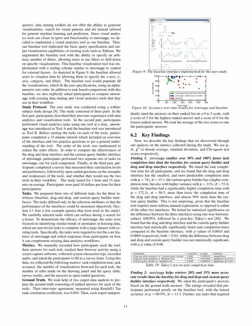
queries; data mining toolkits do not offer the ability to generatevisualizations, search for visual patterns and are instead tailoredfor general machine learning and prediction. Since visual analyt-ics tools are closer in spirit and functionality to zenvisage, we de-cided to implement a visual analytics tool as our baseline. Thus,our baseline tool replicated the basic query specification and out-put visualization capabilities of existing tools such as Tableau. Weaugmented the baseline tool with the ability to specify an arbi-trary number of filters, allowing users to use filters to drill-downon specific visualizations. This baseline visualization tool was im-plemented with a styling scheme similar to zenvisage to controlfor external factors. As depicted in Figure 9, the baseline allowedusers to visualize data by allowing them to specify the x-axis, y-axis, category, and filters. The baseline tool would populate allthe visualizations, which fit the user specifications, using an alpha-numeric sort order. In addition to task-based comparisons with thisbaseline, we also explicitly asked participants to compare zenvis-age with existing data mining and visual analytics tools that theyuse in their workflow.Study Protocol. The user study was conducted using a within-subject study design [9]. The study consisted of three parts. In thefirst part, participants described their previous experience with dataanalytics and visualization tools. In the second part, participantsperformed visual analytics tasks using one tool at a time. zenvis-age was introduced as Tool A and the baseline tool was introducedas Tool B. Before starting the tasks on each of the tools, partici-pants completed a 15-minute tutorial which included an overviewof the interface and two practice questions to get a general under-standing of the tool. The order of the tools was randomized toreduce the order effects. In order to compare the effectiveness ofthe drag and drop interface and the custom query builder interfaceof zenvisage, participants performed two separate sets of tasks onzenvisage, one for each component. Finally, in the third part, par-ticipants completed a survey that measured their satisfaction levelsand preferences, followed by open-ended questions on the strengthsand weaknesses of the tools, and whether they would use the twotools in their workflow. The study lasted for 1 hour and 15 min-utes on average. Participants were paid 10 dollars per hour for theirparticipation.Tasks. We prepared three sets of different tasks for the three in-terfaces (baseline, drag and drop, and custom query builder inter-faces). The tasks differed only in the selection attributes so that theperformance of the interfaces could be measured objectively (Sec-tion 4.1 lists a few example queries that were used in the study).We carefully selected tasks which can surface during a search fora house. To demonstrate the efficacy of zenvisage, the tasks werefocused on identifying similar trends or anomalies in housing data,which are non-trivial tasks to complete with a large dataset with ex-isting tools. Specifically, the tasks were targeted to test the core fea-tures of zenvisage and solicit responses from participants on howit can complement existing data analytics workflows.Metrics. We manually recorded how participants used the tool,their answers for each task, tracked their browser activity using ascreen capture software, collected system interaction logs, recordedaudio, and asked the participants to fill in a survey form. Using thisdata, we collected the following metrics: task completion time, taskaccuracy, the number of visualizations browsed for each task, thenumber of edits made on the drawing panel and the query table,survey results, and the answers to open-ended questions.Ground Truth. We took help of two expert data analysts to pre-pare the ground truth consisting of ranked answers for each of thetasks. Their inter-rater agreement, measured using Kendall's Taurank correlation coefficient, was 0.854. Then, each expert indepen-

Figure 9: The baseline interface implemented for the user study.

0 50 100 150 200 250 300time (ms)

0

20

40

60

80

100

accu

racy

%

zenvisage drag and drop interfacezenvisage custom query builderBaseline

Figure 10: Accuracy over time results for zenvisage and baseline

dently rated the answers on their ranked list on a 0 to 5 scale, witha score of 5 for the highest ranked answer and a score of 0 for thelowest ranked answer. We took the average of the two scores to ratethe participants' answers.

6.2 Key FindingsNow, we describe the key findings that we discovered through

our analysis on the metrics collected during the study. We use µ ,σ , χ2 to denote average, standard deviation, and Chi-square testscores respectively.Finding 1: zenvisage enables over 50% and 100% faster taskcompletion time than the baseline for custom query builder anddrag and drop interface respectively. We timed the task comple-tion time for all participants, and we found that the drag and dropinterface has the smallest, and most predictable completion timewith µ = 74s, σ = 15.1, the custom query builder has a higher com-pletion time, but also with higher variance with µ = 115s, σ = 51.6,while the baseline had a significantly higher completion time withµ = 172.5s, σ = 50.5, more than twice the completion time ofthe drag and drop interface, and almost 50% more than the cus-tom query builder. This is not surprising, given that the baselinetool requires more tedious manual exploration, as opposed to eitherof the other two interfaces. We tested for statistical significance onthe difference between the three interfaces using one-way between-subject ANOVA, followed by a post-hoc Tukey’s test [46]. Wefound that the drag and drop interface and the custom query builderinterface had statistically significantly faster task completion timescompared to the baseline interface, with p values of 0.0010 and0.0069 respectively, both < 0.01, while the difference between dragand drop and custom query builder was not statistically significant,with a p value of 0.06.

Treatments Q statistic p-value inferenceDrag and drop interface vs. Custom query builder 3.3463 0.0605331 insignificantDrag and drop interface vs. Baseline tool 7.9701 0.0010053 significant (p<0.01)Custom query builder vs. Baseline tool 4.6238 0.0069276 significant (p<0.01)

Table 19: Tukey’s test on task completion time

Finding 2: zenvisage helps retrieve 20% and 35% more accu-rate results than the baseline for drag and drop and custom querybuilder interface respectively. We rated the participant’s answersbased on the ground truth answers. The ratings revealed that par-ticipants performed poorly on the baseline tool, with the lowestaccuracy of µ = 69.9%, σ = 13.3. Further, any tasks that required

11

comparing multiple pairs of visualizations or trends ended up hav-ing lower accuracy than those that looked for a pattern, such as apeak or an increasing trend, in a single visualization. Overall thelow accuracy can be attributed to the fact that the participants gottired of browsing through large collections of visualizations and re-turn the first result that approximately matches the conditions. Onthe other hand, since zenvisage is able to accept more fine-graineduser input, and rank output visualizations, participants were ableto retrieve accurate answers with less effort. Among the two inter-faces in zenvisage, while the drag and drop interface, as we sawearlier, had a faster task completion time, it also had lower accu-racy: µ = 85.3%, σ = 7.61. The custom query builder had thehighest accuracy: µ = 96.3%, σ = 5.82. Thus accuracy is greaterthan the baseline by over 20% (for the drag and drop interface) orover 35% (for the custom builder interface). Finally, looking atboth accuracy and task completion times together in Figure 10, wecan conclude that zenvisage helps in “fast-forwarding to desiredvisualizations” with high accuracy.Finding 3: The drag and drop interface, and the custom querybuilder complement each other. The large majority of participants(8/12) mentioned that the drag and drop interface, and the customquery builder complement each other in making zenvisage power-ful in searching for specific insights. About 25 percent (3/12) ofthe participants (all with backgrounds in machine learning and datamining) preferred using only the custom query builder while justone participant (with no prior experience with query languages orprogramming languages) found only the drag and drop interface asuseful. Participants stated that they would use the drag and dropinterface for exploration and simple pattern search, and the customquery builder for specific and complex queries. One participantstated: “When I know what I am looking for is something exact, Iwant to use the query table. The other one [drag and drop inter-face] is for exploration when you are not so sure.” We next discussthe participants'responses to the individual components of zenvis-age.Finding 4: The drag and drop interface is intuitive. Participantsliked the simplicity and intuitiveness of the drag and drop interface.One stated: “[The drawing feature] is very easy and intuitive, I candraw the trend and automatically get the results.” The participantsrated the usability of this feature on a 5-point Likert scale rang-ing from strongly disagree (1) to strongly agree (5), and found thedrawing feature easy to use, with µ = 4.45, σ = 0.674. Despite thepositive feedback, participants did identify limitations, specificallythat the functionality is restricted to identifying trends similar to asingle hand-drawn trend.Finding 5: The custom query builder is useful for complex queries.The majority of the participants (11/12) said that the custom querybuilder allowed them to search for complex insights which mightbe difficult to answer in the drag and drop interface. When askedif the custom query builder is comparatively difficult to the drag-and-drop interface, participants tended to agree, with µ = 3.73,σ = 0.866 on a 5-point scale (5 is strongly agree). At the same time,participants acknowledged the flexibility and the efficacy supportedby the custom query builder. One participant explicitly stated thatthey preferred the custom query builder over the drag and drop in-terface for this reason: “When the query is very complicated, [thedrag and drop interface] has its limitations, so I think I will usethe query table most of the times unless I want to get a brief im-pression.” Another participant stated that the custom query builder“has more functionality and it lets me express what I want to doclearly more than the sketch”. This is consistent with other re-sponses. Participants with a background in machine learning, datamining, and statistics (3/12) preferred always using the custom

query builder over the drag and drop interface.Finding 6: zenvisage is much more effective (4.27 vs. 2.67 on a 5point scale) than the baseline tool at visual data exploration, andwould be a valuable addition to the participants’ analytics work-flow. In response to survey question “I found the tool to be effectivein visualizing the data I want to see”, the participants rated zenvis-age (drag and drop interface + custom query builder) much higher(µ = 4.27, σ = 0.452) than the baseline tool (µ = 2.67, σ = 0.890)on a 5 point Likert scale. A participant experienced in Tableau com-mented:“In Tableau, there is no pattern searching. For example, ifI see some pattern in Tableau, such as a decreasing pattern, andI want to see if any other variable is decreasing in that month, Ihave to go one by one to find this trend. But here I can find thisthrough the query table.”. When asked about using the two toolsin their current workflow, 9/12 participants stated that they woulduse zenvisage in their workflow, whereas only 2/12 participantsstated that they would use our baseline tool (χ2 = 8.22, p<0.01).When the participants were asked how they would use zenvisagein their workflow, one participant provided a specific scenario: “IfI am doing my social science study and I want to see some specificbehavior among users, then I can use tool A [zenvisage ] since Ican find the trend I am looking for and easily see what users fitinto the pattern.” Other participants mentioned that they would usethis tool for finding outliers during data cleaning, finding commonpatterns, and gaining an initial understanding of data distributionbefore running a machine learning task. Participants found no par-ticular reason to use the baseline tool, since (as one participant putit) “the existing solutions can already do what tool B can do.”Finding 7: zenvisage can be improved. While the participantslooked forward to using the custom query builder in their ownworkflow, a few of them were interested in directly exposing thecommonly-used trends/patterns such as outliers, through the dragand drop interface. Some of them were interested in knowing howthey could integrate custom functional primitives (we could notcover it in the tutorial due to time constraints). In order to improvethe user experience, participants suggested adding instructions andguidance for new users as part of the interface. Participants alsocommented on the unrefined look and feel of the tool, as well as thelack of the diverse set of usability related features, such as book-marking and search history, that are offered in existing systems.

7. RELATED WORKOur work is related to prior work in a number of areas.

Visual Analytics Tools: A number of interactive data analyticstools have been developed, such as ShowMe, Polaris, Spotfire, andTableau [45, 44, 33, 8]. Here, the onus is on the user to specify thevisualization to be generated, and then repeat until the desired vi-sualization is identified. Similar specification tools have also beenintroduced by the database community[18, 30, 31, 25]. zenvisageis related to work on browsing data cubes—finding explanations,getting suggestions for cubes to visit, or identifying generalizationsfrom a single cube, e.g., [39, 40]. While we may be able to reuse themetrics from that line of work, the same techniques will not directlyapply to the identification of trends, patterns, and anomalies for in-teractive visualizations. Specifically, no OLAP techniques capturethe interestingness of slices of the data cube that can be visualizedvia two (or more) dimensional visualizations: instead, the focus ismore on raw aggregate data, on interestingness of cells of the cube,displayed within multidimensional tables. Thus, the emphases aredifferent. Indeed, we believe that, given the popularity of tools likeTableau, users prefer to browse and explore data visually ratherthan in tables. There has been some work sketch-based interfaces

12

for visualization [21, 47, 22, 10]: however, none of this work ad-dresses the deep scalability issues at play if these techniques are tobe applied on large datasets. There is limited work on visual queryinterfaces [34, 23, 52, 6], but the goal there is to make it easier topose SQL queries.Anomaly Discovery: Anomaly detection is a well-studied topic [14,7, 37]. Our goal in that zenvisage is expected to be interactive, es-pecially on large datasets; most work in anomaly detection focuseson accuracy at the cost of latency and is typically a batch operation.In our case, since interactiveness is of the essence, and requests cancome at any time, the emphasis is on scalable on-the-fly data pro-cessing aspects.Time Series Similarity and Indexing: There has been some workon indexing of of time series data, e.g., [29, 19, 13, 28, 11, 17, 27];for the attributes that are queried frequently, we plan to reuse thesetechniques for similarity search. For other attributes, indexing andmaintaining all trends is impossible, since the number of trendsgrows exponentially with the number of indexed attributes.Visualization Recommendation Tools: There has been some re-cent work on building systems that recommend visualizations toanalysts. Voyager [51] recommends visualizations based on aes-thetic properties of the visualizations, as opposed to user queries.SeeDB [36] recommends visualizations that best display the dif-ference between two sets of data. Both SeeDB and Voyager canbe seen to be special cases of zenvisage, since zenvisage can beviewed to be a user-driven visualization recommendation engine aswell. The optimization techniques outlined are a generalization ofthe techniques described in SeeDB; while the techniques in SeeDBare special-cased to the query considered (a simple comparativequery), here, our goal is to support and optimize all ZQL queries.Data Mining Query Languages: There has been some limitedwork in the space of data mining query languages, all from the early90s, focusing either on association rule mining (languages such asDMQL [20] and MSQL [24]), or on storing and retrieving modelson data (languages such as OLE DB [35]), as opposed to a visualexploration language like ZQL.Multi-Query Optimization: Our proposed primitive query opti-mization techniques are currently tailored to the zenvisage setting,specifically trying to identify opportunities for batching of individ-ual visualization generation SQL queries so as to “combine work”as much as possible, even before they are issued to the database.These optimization techniques are external to the database system,are completely interpreted based on the rows of ZQL, and do notrequire any modifications to the underlying database. Indeed, thereare very powerful multi-query optimization techniques in relatedwork, e.g., [41, 42, 16, 38, 26], that we plan to leverage as futurework to further improve the performance of zenvisage, when we at-tempt to holistically process ZQL queries by making modificationsto the underlying database query processor, rather than simply op-erating as a “wrapper” on top of a database.

8. CONCLUSIONWe propose zenvisage, a tool for effortless specification and vi-

sualization of interesting patterns and insights from large datasets.The bulk of our paper focused on the formal specification of ZQL,our query language; we described how ZQL captures a range of in-teresting and useful scenarios, and is powerful enough to capture allof the typical data exploration queries users wish to issue. We thendescribed three simple optimizations for translating ZQL queriesinto SQL queries, and demonstrated how these optimizations leadto several orders of performance improvement on real and syntheticdatasets. Finally, we presented a user study that demonstrated theusability and effectiveness of zenvisage. Our ZQL prototype is

fully functional and allows both novice and expert users to issueZQL queries. While our work is a promising first step towards sim-plifying and improving visual data exploration, much more workremains to be done in further improving optimization. Learningfrom user feedback and providing better recommendations are alsointeresting questions that are worth pursuing.

AcknowledgementWe acknowledge support from grant IIS-1513407 awarded by theNational Science Foundation, grant 1U54GM114838 awarded byNIGMS and 3U54EB020406-02S1 awarded by NIBIB through fundsprovided by the trans-NIH Big Data to Knowledge (BD2K) ini-tiative (www.bd2k.nih.gov), and the Faculty Research Award pro-vided by Google. We thank Edward Xue, Xiaofo Yu, Lijin Guo,Weijia Luo, and the data-people group at University of Illinois fortheir contribution to zenvisage and its developments. The contentis solely the responsibility of the authors and does not necessarilyrepresent the official views of the funding agencies and organiza-tions.

9. REFERENCES[1] Airline dataset. [Online; accessed 30-Oct-2015].[2] Census income dataset. [Online; accessed 30-Oct-2015].[3] Spotfire, http://spotfire.com. [Online; accessed 17-Aug-2015].[4] Tableau public. [Online; accessed 3-March-2014].[5] Zillow real estate data. [Online; accessed 1-Feb-2016].[6] A. Abouzied, J. M. Hellerstein, and A. Silberschatz. Playful query

specification with dataplay. PVLDB, 5(12):1938–1941, 2012.[7] M. Agyemang, K. Barker, and R. Alhajj. A comprehensive survey of

numeric and symbolic outlier mining techniques. Intell. Data Anal.,10(6):521–538, Dec. 2006.

[8] C. Ahlberg. Spotfire: An information exploration environment.SIGMOD Rec., 25(4):25–29, Dec. 1996.

[9] K. S. Bordens and B. B. Abbott. Research design and methods: Aprocess approach . McGraw-Hill, 2002.

[10] P. Buono, A. Aris, C. Plaisant, A. Khella, and B. Shneiderman.Interactive pattern search in time series. In Electronic Imaging 2005,pages 175–186. International Society for Optics and Photonics, 2005.

[11] K. Chakrabarti, E. Keogh, S. Mehrotra, and M. Pazzani. Locallyadaptive dimensionality reduction for indexing large time seriesdatabases. ACM Trans. Database Syst., 27(2):188–228, June 2002.

[12] S. Chambi, D. Lemire, O. Kaser, and R. Godin. Better bitmapperformance with roaring bitmaps. Software: Practice andExperience, 2015.

[13] K.-P. Chan and A.-C. Fu. Efficient time series matching by wavelets.In Data Engineering, 1999. Proceedings., 15th InternationalConference on, pages 126–133, Mar 1999.

[14] V. Chandola, A. Banerjee, and V. Kumar. Anomaly detection: Asurvey. ACM Comput. Surv., 41(3):15:1–15:58, July 2009.

[15] J. W. Creswell and V. L. P. Clark. Designing and conducting mixedmethods research. 2007.

[16] N. N. Dalvi, S. K. Sanghai, P. Roy, and S. Sudarshan. Pipelining inmulti-query optimization. Journal of Computer and System Sciences,66(4):728–762, 2003.

[17] C. Faloutsos, M. Ranganathan, and Y. Manolopoulos. Fastsubsequence matching in time-series databases. SIGMOD Rec.,23(2):419–429, May 1994.

[18] H. Gonzalez et al. Google fusion tables: web-centered datamanagement and collaboration. In SIGMOD Conference, pages1061–1066, 2010.

[19] D. Gunopulos and G. Das. Time series similarity measures and timeseries indexing (abstract only). SIGMOD Rec., 30(2):624–, May2001.

[20] J. Han, Y. Fu, W. Wang, K. Koperski, O. Zaiane, et al. Dmql: A datamining query language for relational databases. In Proc. 1996SiGMOD, volume 96, pages 27–34, 1996.

13

[21] H. Hochheiser and B. Shneiderman. Visual specification of queriesfor finding patterns in time-series data. In Proceedings of discoveryscience, pages 441–446, 2001.

[22] H. Hochheiser and B. Shneiderman. Dynamic query tools for timeseries data sets: timebox widgets for interactive exploration.Information Visualization, 3(1):1–18, 2004.

[23] S. Idreos and E. Liarou. dbtouch: Analytics at your fingertips. InCIDR 2013, Sixth Biennial Conference on Innovative Data SystemsResearch, Asilomar, CA, USA, January 6-9, 2013, OnlineProceedings, 2013.

[24] T. Imielinski and A. Virmani. A query language for database mining.Data Mining and Knowledge Discovery, 3(4):373–408, 2000.

[25] S. Kandel, R. Parikh, A. Paepcke, J. M. Hellerstein, and J. Heer.Profiler: integrated statistical analysis and visualization for dataquality assessment. In AVI, pages 547–554, 2012.

[26] A. Kementsietsidis, F. Neven, D. V. de Craen, and S. Vansummeren.Scalable multi-query optimization for exploratory queries overfederated scientific databases. PVLDB, 1(1):16–27, 2008.

[27] E. Keogh. A decade of progress in indexing and mining large timeseries databases. In Proceedings of the 32Nd InternationalConference on Very Large Data Bases, VLDB ’06, pages 1268–1268.VLDB Endowment, 2006.

[28] E. Keogh, K. Chakrabarti, M. Pazzani, and S. Mehrotra.Dimensionality reduction for fast similarity search in large timeseries databases. Knowledge and Information Systems, 3(3):263–286,2001.

[29] E. Keogh, K. Chakrabarti, M. Pazzani, and S. Mehrotra. Locallyadaptive dimensionality reduction for indexing large time seriesdatabases. SIGMOD Rec., 30(2):151–162, May 2001.

[30] A. Key, B. Howe, D. Perry, and C. Aragon. Vizdeck: Self-organizingdashboards for visual analytics. SIGMOD ’12, pages 681–684, 2012.

[31] M. Livny et al. Devise: Integrated querying and visualization of largedatasets. In SIGMOD Conference, pages 301–312, 1997.

[32] J. Mackinlay. Automating the design of graphical presentations ofrelational information. ACM Trans. Graph., 5(2):110–141, Apr. 1986.

[33] J. D. Mackinlay et al. Show me: Automatic presentation for visualanalysis. IEEE Trans. Vis. Comput. Graph., 13(6):1137–1144, 2007.

[34] A. Nandi, L. Jiang, and M. Mandel. Gestural query specification.PVLDB, 7(4):289–300, 2013.

[35] A. Netz, S. Chaudhuri, U. Fayyad, and J. Bernhardt. Integrating datamining with sql databases: Ole db for data mining. In DataEngineering, 2001. Proceedings. 17th International Conference on,pages 379–387. IEEE, 2001.

[36] A. Parameswaran, N. Polyzotis, and H. Garcia-Molina. SeeDB:Visualizing Database Queries Efficiently. Stanford Infolab, 2013.

[37] A. Patcha and J.-M. Park. An overview of anomaly detectiontechniques: Existing solutions and latest technological trends.Comput. Netw., 51(12):3448–3470, Aug. 2007.

[38] P. Roy, S. Seshadri, S. Sudarshan, and S. Bhobe. Efficient andextensible algorithms for multi query optimization. In ACMSIGMOD Record, volume 29, pages 249–260. ACM, 2000.

[39] S. Sarawagi. Explaining differences in multidimensional aggregates.In VLDB, pages 42–53, 1999.

[40] G. Sathe and S. Sarawagi. Intelligent rollups in multidimensionalolap data. In VLDB, pages 531–540, 2001.

[41] T. K. Sellis. Multiple-query optimization. ACM TODS, 13(1):23–52,1988.

[42] K. Shim, T. Sellis, and D. Nau. Improvements on a heuristicalgorithm for multiple-query optimization. Data & KnowledgeEngineering, 12(2):197–222, 1994.

[43] M. Slee, A. Agarwal, and M. Kwiatkowski. Thrift: Scalablecross-language services implementation. Facebook White Paper,5(8), 2007.

[44] C. Stolte et al. Polaris: a system for query, analysis, and visualizationof multidimensional databases. CACM, 51(11):75–84, 2008.

[45] C. Stolte et al. Polaris: a system for query, analysis, and visualizationof multidimensional databases. Commun. ACM, 51(11):75–84, 2008.

[46] J. W. Tukey. Comparing individual means in the analysis of variance.Biometrics, pages 99–114, 1949.

[47] M. Wattenberg. Sketching a graph to query a time-series database. InCHI ’01 Extended Abstracts on Human Factors in Computing

Systems, CHI EA ’01, pages 381–382, New York, NY, USA, 2001.ACM.

[48] H. Wickham. ggplot: An implementation of the grammar of graphics.R package version 0.4. 0, 2006.

[49] Wikipedia. Statistical distance — wikipedia, the free encyclopedia,2013. [Online; accessed 16-July-2013].

[50] L. Wilkinson. The grammar of graphics. Springer Science &Business Media, 2006.

[51] K. Wongsuphasawat, D. Moritz, A. Anand, J. Mackinlay, B. Howe,and J. Heer. Voyager: Exploratory analysis via faceted browsing ofvisualization recommendations. IEEE Trans. Visualization & Comp.Graphics, 2015.

[52] M. M. Zloof. Query-by-example: A data base language. IBM SystemsJournal, 16(4):324–343, 1977.

APPENDIXA. QUERY LANGUAGE FORMALIZATION:

ADDITIONAL DETAILSIn this section, we present some additional details on our formal-

ization that we did not cover in the main body of the paper.

A.1 Additional Details on X and Y ColumnsIn addition to using a single attribute for an X or Y column, ZQL

also allows the use of the Polaris table algebra [44] in the X and Ycolumns to to arbitrarily compose multiple attributes into a singleattribute; all three operators are supported: +,×, /. Table 20 showsan example of using the + operator to visualize both profits andsales on a single y-axis. Note that this is different from the examplegiven in Table 4, which generates two visualizations, as opposed toa single visualization. An example using both table algebra and setsis given in Table 21, which uses the × operator to return the set ofvisualizations which measures the sales for the Cartesian productof ‘product’ and one of ‘county’, ‘state’, and ‘country’.

Name X Y Constraints*f1 ‘product’ ‘profit’ + ‘sales’ location=‘US’

Table 20: A ZQL query for a visualization which depicts both prof-its and sales on the y-axis for products in the US.

Name X Y*f1 ‘product’ × (x1 in {‘county’, ‘state’, ‘country’}) ‘sales’

Table 21: A ZQL query for the set of visualizations which measuresthe sales for one of (‘product’, ‘county’), (‘product’, ‘state’), and(‘product’, ‘country’).

A.2 Additional Details on the Z ColumnZQL also allows the iteration over attributes in the Z column as

shown in Table 22. The result of this query is the set of all sales overtime visualizations for every possible slice in every dimension ex-cept ‘time’ and ‘sales’. Since both attribute and attribute value canvary in this case, we need separate variables for each component,and the full attribute name, value pair (z1.v1) must be specified.Note that the resulting set of visualizations comes from the Carte-sian product of possible attribute and attribute value pairs. The first* symbol refers to all possible attributes, while the second * symbolrefers to all possible attribute values given an attribute. If the userwishes to specify specific subsets of attribute values for attributes,she must name them individually. An example of this is given inTable 23 where the z1 and v1 iterate over the pairs {(‘product’,‘chair’), (‘product’, ‘desk’), (‘location’, ‘US’)}.

Name X Y Z*f1 ‘year’ ‘sales’ z1.v1 <– (* \ {‘year’, ‘sales’}).*

Table 22: A ZQL query which returns the set of sales over yearvisualizations for each attribute that is not time or sales.

14

Figure 11: Custom query builder with bar charts Figure 12: Custom query builder with scatterplots

Finally, it is possible to have multiple Z columns, named Z2, Z3,. . . in ZQL, increasing the number of ways of simultaneously slic-ing through the data—these Z columns would be akin to layers inPolaris. These multiple Z columns enable us to increase the spaceof candidate visualizations by letting us derive a Cartesian productfor the z-axis. Table 24 gives an example of using an additional Zcolumn. The query is used to slice the data in two ways: one interms of the products and one in terms of the year. The resultingset of visualizations could potentially then be used to generate com-parison sales over time visualizations between USA and Canada foritems whose sales differed the most between USA and Canada.

X Y Z‘year’ ‘sales’ z1.v1 <– (‘product’.{‘chair’, ‘desk’} | ‘location’.‘US’)

Table 23: A ZQL query which returns a set of sales over year visu-alizations; one for chairs, one for desks, and one for items sold inthe US. (Name is not displayed above.)

X Y Z Z2‘year’ ‘sales’ v1 <– ‘product’.* v2 <– ‘location’.{USA, Canada}

Table 24: A ZQL query which returns the set of sales over yearvisualizations for each product in USA and Canada (Name is notdisplayed above.)

A.3 Additional Details on the Constraints Col-umn

Beyond the reasons described previously, there are a few ad-ditional ways the constraints column differs from the Z column.When ZQL returns the data which the zenvisage front-end uses torender actual visualizations with, the values for the Z columns arereturned as part of the output. This is usually necessary as the Zcolumn often iterates over a set of values, so the values for the Zcolumn must be returned for proper identification as to which partof the returned data belongs to which slice. The results of the Con-straints column, however is not returned as an output of ZQL.

Secondly, because of the restrictions we have put on the Con-straints column, we can allow the Constraints column to be muchmore complex than the Z columns. Earlier, we saw that we re-quired extra Z columns to be able to deal with more than one at-tribute in the z-axis, but with the Constraints column, all of thoseconstraints can be combined in one single column. The best wayto think about the Constraints column is to imagine that the expres-sion in the Constraints column will simply be added conjunctivelyto the WHERE clause of the translated SQL queries. In fact, thesyntax for the Constraints column has been adjusted so that the ex-pression can be taken from a ZQL table and directly added to SQL.For example, there is no need to quote attributes in the Constraintscolumn. As a result, the set of possible values for the Constraintsclause is roughly equal to the set of possible expressions for theWHERE clause in SQL. An example which makes extensive useof the Constraints column is given by Table 25.

Name X Y Constraints*f1 ‘time’ ‘sales’ product=‘chair’ AND zip LIKE ‘02\d{3}’

Table 25: A ZQL query for a sales over time visualization for chairssold in the US in zip codes between 02000 and 02999.

A.4 Additional Details on the Viz ColumnLike other columns, the Viz column also supports sets of val-

ues and iteration over those sets. Table 26 refers to a ZQL querywhich iterates over various binning sizes for the x-axis. Table 27iterates over the types of visualizations using t1. Note, unlike theZ column, we do not need to create a variable to iterate over thesummarization even though the visualization type changes, sincethe same summarization is valid for both types.

Although the bar chart and dot plot does not take in any param-eters, other types of charts, such as the box plot, may take in ad-ditional parameters (e.g., to determine where the whisker shouldend); these additional parameters may be added as part of the sum-marization.

A.5 Additional Details on the Process ColumnEven with the primitives defined in the paper so far, sometimes

the user would like to be able to write her own. ZQL supportsuser-defined functions that are executed by the zenvisage back-end. User-defined functions may take in name and axis variablesand perform whatever computation is necessary; zenvisage treatsthem as black boxes. However, users are encouraged to use theprimitives defined by ZQL as they allow the zenvisage back-endmore opportunities for optimization.

Furthermore, although visual components typically outnumberprocesses, there may occur cases in which the user would like tospecify multiple processes in one line. To accomplish this, the usersimply delimits each process with a comma and surrounds eachdeclaration of variables with parentheses. Table 28 gives an exam-ple of this.

B. QUERY EXECUTION: NAIVE TRANS-LATION LISTING

Here, we list the pseudocode for the naive translation for queryexecution for reference.

Listing 1: Pseudocode for the compiled query in Table 14# Row 1v1_range = P,f1 = make_array(1, size(v1_range))for v1 in [0 .. size(v1_range)]:f1[v1] = sql(‘‘SELECT year, SUM(sales)

WHERE product=‘%s’ and location=‘US’GROUP BY year ORDER BY year’’),

v1_range[v1])v2_range = []for v1 in [0 .. size(v1_range)]:

15

Name X Y Viz*f1 ‘weight’ ‘sales’ s1 <– bar.{(x=bin(20), y=agg(‘sum’)), (x=bin(30), y=agg(‘sum’)), (x=bin(40), y=agg(‘sum’))}

Table 26: A ZQL query which returns the bar charts of overall sales for different weight classes, for varying weight class sizes.Name X Y Viz

*f1 ‘weight’ ‘sales’ t1 <– {bar, dotplot}.(x=bin(20), y=agg(‘sum’))Table 27: A ZQL query which returns the set of bar chart and dot plot of overall sales for different weight classes.

Name X Y Z Process-f1f2 ‘year’ ‘sales’ v1 <– ‘product’.* (v2 <– argmaxv1[k = 1]D( f 1, f 2)), (v3 <– argminv1[k = 1]D( f 1, f 2))

*f3 ‘year’ ‘sales’ v2*f4 ‘year’ ‘sales’ v3

Table 28: A ZQL query which returns the sales over years visualizations for the product that looks most similar to the user-drawn input andmost dissimilar to the user-drawn input.

if T(f1[v1]) > 0:v2_range.append(v1_range[v1])

# Row 2f2 = make_array(1, size(v1_range))for v1 in [0 .. size(v1_range)]:f2[v1] = sql(‘‘SELECT year, SUM(sales)

WHERE product=‘%s’ and location=‘UK’GROUP BY year ORDER BY year’’),

v1_range[v1])v3_range = []for v1 in [0 .. size(v1_range)]:if T(f2[v1]) < 0:v3_range.append(v1_range[v1])

# Row 3v4_range = union(v2_range, v3_range)f3 = make_array(1, size(v4_range))for v4 in [0 .. size(v4_range)]:f3[v4] = sql(‘‘SELECT year, SUM(profit)

WHERE product=‘%s’GROUP BY year ORDER BY year’’),

v4_range[v4])

return f3

C. ADDITIONAL COMPLETE EXAMPLESTo demonstrate the full expressive power of ZQL, we present

four realistic, complex example queries. We show that even withcomplicated scenarios, the user is able to capture the insights shewants with a few meaningful lines of ZQL.Query 1. The stapler has been one of the most profitable productsin the last years for GlobalMart. The Vice President is interested inlearning about other products which have had similar profit trends.She wishes to see some representative sales over the years visual-izations for these products.

Table 29 shows what the query that the Vice President wouldwrite for this scenario. She first filters down to the top 100 prod-ucts which have the most similar to profit over year visualizationsto that of the stapler’s using the argmin in the second row. Then,from the resulting set of products, v2, she picks the 10 most repre-sentative set of sales over visualizations using R, and displays thosevisualizations in the next line with f4. Although the Vice Presidentdoes not specify the exact distance metric for D or specify the exactalgorithm for R, she knows zenvisage will select the most reason-able default based on the data.Query 2. The Vice President, to her surprise, sees that there afew products whose sales has gone up over the last year, yet theirprofit has declined. She also notices some product’s sales havegone down, yet their profit has increased. To investigate, the Vice

President would like to know about the top 10 products who havethe most discrepancy in their sales and profit trends, and she wouldlike to visualize those trends.

This scenario can be addressed with the query in Table 30. TheVice President names the set of visualizations for profit over monthf1 and the sales over month visualizations f2. She then comparesthe visualizations in the two set using the argmax and retrieves thetop 10 products whose visualizations are the most different. Forthese visualizations, she plots both the sales and profit over months;y1 <– {‘sales’, ‘profit’} is a shortcut to avoid having to separatesrows for sales and profit. Note that the Vice President was carefulto constrain ZQL to only look at the data from 2015.Query 3. The Vice President would like to know more about thedifferences between a product whose sales numbers do not changeover the year and a product that has the largest growth in the num-ber of sales. To address this question, she writes the query in Ta-ble 31. The first R function call returns the one product whosesales over year visualization is most representative for all products;in other words, v2 is set to the product that has the most averagenumber of sales. The task in the second row selects the product v3which has the greatest upward trending slope T for sales. Finally,the Vice President tries to finds the y-axes which distinguish thetwo products the most, and visualizes them. Although we know v2and v3 only contain one value, they are still sets, so argmax mustiterate over them and output corresponding values v4 and v5.Query 4: Finally, the Vice President wants to see a pair of dimen-sions whose correlation pattern (depicted as a scatterplot) is themost unusual, compared to correlation patterns of other pairs of at-tributes. To address this question, she writes the query in Table 32.She keeps the Z column empty as she does not want to slice thedata. Both X and Y refer to a set M consisting of all the attributesin the dataset she wishes to explore. The task in the second rowselects the X and Y attributes whose sum of distances from othervisualizations (generated by considering all pairs of attributes)is themaximum.

D. EXPRESSIVENESSSo far, we have described, via a collection of examples, the vari-

ous types of queries that can be posted using ZQL. A natural ques-tion now arises: how can we characterize the space of queries ex-pressible via ZQL? In this section, we provide both intuition forthe space of queries expressible via ZQL, as well as more formalarguments. Note, however, that ZQL provides considerable flexi-bility to the user, specifically via the Process and the Viz column;as a result, there may be uses of ZQL we still haven’t foreseen, andthus, our arguments will be necessarily incomplete.

D.1 Formalized CapabilitiesWe now discuss the capabilities of ZQL more formally. For the

rest of our discussion, we will assume that the Viz column uses a

16

Name X Y Z Viz Processf1 ‘year’ ‘profit’ ‘product’.‘stapler’ bar.(y=agg(‘sum’))f2 ‘year’ ‘profit’ v1 <– ‘product’.(* \ {‘stapler’}) bar.(y=agg(‘sum’)) v2 <– argminv1[k = 100]D( f 1, f 2)f3 ‘year’ ‘sales’ v2 bar.(y=agg(‘sum’)) v3 <– R(10,v2, f 3)

*f4 ‘year’ ‘sales’ v3 bar.(y=agg(‘sum’))Table 29: The ZQL query which returns 10 most representative sales over year visualizations for products which have similar profit overyear visualizations to that of the stapler’s.

Name X Y Z Constraints Viz Processf1 ‘month’ ‘profit’ v1 <– ‘product’.* year=2015 bar.(y=agg(‘sum’))f2 ‘month’ ‘sales’ v1 year=2015 bar.(y=agg(‘sum’)) v2 <– argmaxv1[k = 10]D( f 1, f 2)

*f3 ‘month’ y1 <– {‘sales’, ‘profit’} v2 year=2015 bar.(y=agg(‘sum’))Table 30: The ZQL query which returns the sales over month and profit over month visualizations for 2015 for the top 10 products whichhave the biggest discrepancies in their sales and profit trends.

Name X Y Z Viz Processf1 ‘year’ ‘sales’ v1 <– ‘product’.* bar.(y=agg(‘sum’)) v2 <– R(1,v1, f 1)f2 ‘year’ y1 <– M v2 bar.(y=agg(‘sum’)) v3 <– argmaxv1[k = 1]T ( f 1)f3 ‘year’ y1 v3 bar.(y=agg(‘sum’)) y2,v4,v5 <– argmaxy1,v2,v3[k = 10]D( f 2, f 3)

*f4 ‘year’ y2 v6 <– (v4.range | v5.range) bar.(y=agg(‘sum’))Table 31: The ZQL query which returns varying y-axes visualizations where the following two products differ the most: one whose salesnumbers do not change over the year and another which has the largest growth in the number of sales.

Name X Y Z Viz Processf1 x1 <– M y1 <– Mf2 x2 <– M y2 <– M x3,y3 <– argmaxx1,y1[k = 1]sumx2,y2D( f 1, f 2)

*f3 x3 y3 scatterplotTable 32: The ZQL query which returns scatter plot visualization between a pair of attributes whose pattern is most unusual, i.e very differentfrom the patterns made by any other pair of attributes in M.

simple aggregate, as opposed to user-defined interpolation or sum-marization. We will relax this restriction later on in the section.Language Formalization. The ZQL language is straightforwardto describe at a high level. A ZQL query Q is formally defined tobe a collection of expressions E, where each expression2 E can beeither a Visual Component expression V , or a Process expressionP. A Visual Component expression V must contain a tuple of sub-expressions, for each of X ,Y and optionally, Z1,Z2,. . . ,Constraints,Viz. A Process expression P consists of three parts: a ranking func-tion expression S describing how the visualizations must be ranked,a functional expression F describing the computation that deter-mines the ranking, and k, describing how many outputs are desiredfrom the ranking. Thus, formally:

Q := {R} where R :=V |PV := (X ,Y,Z1,Z2, . . . ,Zq,Constraints)P := (S,F,k)

We next describe how V and P are interpreted.Visual Components and Unit Visualizations. To describe how Vis interpreted, we begin with the notion of a unit visualization. Aunit visualization corresponds to a table that is the result of a queryof the following type:

SELECT X, A(Y)FROM R1, R2, ..., RpWHERE ConditionsGROUP BY XORDER BY X

where X, Y, A, Conditions can vary. Thus, a unit visualizationcorresponds to a two-attribute aggregated table. Such two-attributetables can be readily visualized. It is easy to see that the followingholds:

LEMMA D.1. Every visual component generates one or moreunit visualizations.

We define a unit visualization cross-product to be all unit visualiza-tions formed from: combining any Xi in a set of attributes X , anyY j in a set of attributes Y , such that attribute Zi is equated to any at-tribute value vi in a set Vi. These visualizations can be representedusing the following query, where Xi,Y j,v1, ...,vq can vary:2Note that while we enforced that every Process must be associated with a VisualComponent in our tabular interface, it need not be so; this decision was made primarilyfor compactness and intuitiveness. Here, we decouple the two.

SELECT Xi, A(Yj)FROM R1, R2, ..., RpWHERE Z1 = v1 AND ... AND Zq = vq AND ConditionsGROUP BY XiORDER BY Xi

We have the following:

LEMMA D.2. Any unit visualization cross-product can be rep-resented using a visual component.Thus, unit visualizations have close ties to the visual components:essentially, the visual components enable us to assemble a collec-tion of unit visualizations by retrieving data from the database.Visual Component Processor. We now describe how a visualcomponent expression V is processed within zenvisage. To do that,we need to formally define name and axis variables. Name vari-ables are variables that contain an array of unit visualizations. (Asa result, we can say that each name variable corresponds to a se-quence of visualizations.) Axis variables, on the other hand arevariables that contain an array of elements: this could be attributevalues, or names of attributes themselves.

Visual Component Expression

Output Unit Visualizations/Name Variables

Visual Component Processor

Values for Input Axis Variablesu1, u2, …, un f [ … ]

v1[ v11, v12, v13, v14, …, v1m ]v2[ v21, v22, v23, v24, …, v2m ]vk[ vk1, vk2, vk3, vk4, …, vkm ]

…

Output Axis Variables

Process Expression

TaskProcessor

Values for Input Axis Variablesu1, u2, …, un

v1[ v11, v12, v13, v14, …, v1m ]v2[ v21, v22, v23, v24, …, v2m ]vk[ vk1, vk2, vk3, vk4, …, vkm ]

…

Output Axis Variables

Values for Input Name Variablesf1, f2, …, fn

Figure 13: Visual Component Processor Flow (above) Task Pro-cessor Flow (below)

A visual component processor (depicted in Figure 13 (top)) ac-cepts as input a visual component expression V , as well as val-ues for unspecified input axis variables u1, ...,un, within the visualcomponent expression. The output is an instantiation of the namevariable: that is, it is an array of unit visualizations. Additional

17

Figure 14: Patterns in Task Computation (left: star pattern, mid-dle: complete graph pattern, right: bipartite pattern)outputs may include instantiations of output axis variables. (Theseare used to refer to specific aspects or metadata of the unit visual-izations.) For instance, one axis variable vi may hold an array withthe values taken on by attribute Zi for each unit visualization in thename variable array.Task Processor. A task processor takes as a process expression P,as well as values for the unspecified input axis variables u1, ...,un,and unspecified name variables (or arrays of unit visualizations)f1, ..., fm. It then generates instantiations of output axis variables.

Thus, the Task Processor accepts a sequence of unit visualiza-tions as input via name variables, and performs some sub-selection(filtration) and/or ordering on these visualizations. The eventualresult is some subset of the unit visualizations that are provided asinput, ordered in some way. Note that instead of generating an in-stantiation of a single name variable (like the Visual ComponentProcessor), the task processor instantiates multiple axis variables:this distinction is important, because by instantiating multiple axisvariables, these axis variables could be used to generate multiplesets of output unit visualizations via Visual Components. It is therole of the Visual Component Processor to generate the unit visual-izations.Process Primitives. For populating the Process Expression, ZQLprovides a few default functional primitives, including D,T,R. Sincethe process can be overloaded by users to specify their own userdefined functions, it is not clear a-priori what types of computationmay be possible via the Process expression.

Notice however, that all three of D,T,R are computing distanceof some sort: D is explicitly computing a distance between a pairof visualizations, T is checking the overall trend of a visualizationso is computing a distance between a visualization and the trend,R is identifying representatives, and implicitly needs to computedistances between all pairs of visualizations in the collection.

Using these three primitives, and how we’ve used them in queries,we have identified three patterns of distance computation that areexpressible in tasks, and capture all the examples described in thepaper. These patterns are depicted in Figure 14. Each node depictsa visualization, while each edge between two visualizations corre-sponds to a distance computation between them. The pattern onthe left is a star pattern, which compares the distance between acollection of unit visualizations to a reference. This pattern is usedfor queries in Table 2 and Table 8. The pattern in the middle is acomplete graph pattern, where unit visualizations are all comparedagainst each other. This pattern is used for queries in Table 13, Ta-ble 29, and Table 32. Lastly, the pattern on the right is a bipartitegraph pattern, where pairs of corresponding unit visualizations arecompared against each other. This pattern is used for queries inTable 10 and Table 12.Overall Capabilities. Thus, at a high level, zenvisage is tailoredtowards first, enumerating an array of unit visualizations using vi-sual components, and second, task-based computation involvingone of the three patterns displayed in Figure 14, to identify unitvisualizations within this array with desired properties, followedby repetitions of these two above steps.Viz Column. So far, we have assumed that the Viz column uses asimple aggregate for Y : in fact, the Viz column could apply somerestricted set of data transformations, binning in arbitrary ways,

noise removal, and mappings to different types of visualizations,as described in Section 2.1.5. However, as described in that sec-tion, we are directly leveraging the capabilities of the grammar ofgraphics to support these operations.

D.2 Discussion of the Space of Use CasesAs described above, ZQL is targeted at generating simple unit vi-

sualizations via visual components, and then filtrating and orderingthem via tasks, which can be fed as input to other visual compo-nents or output to the user.

The visual components generate unit visualizations: the unit vi-sualizations ZQL is capable of handling correspond to a singleSELECT-FROM-WHERE-GROUPBY-ORDER; complicated nestedqueries are not the target of zenvisage, since they are not usuallythe target of visual data exploration. The tasks computation is lim-ited to selecting visualizations with specific properties from a set:even this encompasses a large collection of use-cases, ranging fromsimilarity and dissimilarity search, or to check if a visualization hasa specific property, to outlier detection and identification of repre-sentatives, to finding differences between corresponding visualiza-tions, as we saw in the previous sections.

This implies that there is a large swath of data mining tasks thatare not captured by ZQL: this includes prediction of any sort, clas-sification, regression, dimensionality reduction, or frequent patternmining. There are other data processing tasks that are not capturedby ZQL, including data cleaning or pre-processing, data integra-tion, or expressing complex queries or computation that don’t cor-respond to the unit visualization template described above.

Data Preparation

Data Exploration

Complex Analytics

Target of Visual Analytics Tools

e.g., Tableau, Excel

Target of Data Cleaning Tools

Target of Machine Learning Packages

Figure 15: The three stages of data analytics currently: the shadedbox is our focus

Indeed, ZQL is not meant to be a one-stop-shop for all of thecomputation on data: it is meant to be the next logical step forcurrent data visualization tools, that severely lack the functionalityof helping users find desired patterns in visualizations or comparevisualizations. This means that the data is already cleaned beforeit is visualized: this is assumed in all data visualization tools. Thisalso means that complex analytics, including prediction or mining,and are not the focus of simple visualization, are better suited forsubsequent tools.

In Figure 15, we depict our conceptualization of the three stagesof data analytics; our target is not the first or the third stages, whichare better handled by other tools. Instead, our focus is on the mid-dle, second stage, which is also the focus of current visual analyticstools.

E. EVALUATING BACK-END DATABASESIn this experiment, we compare the performance between our

two database back-ends: PostgreSQL and the in-memory Roar-ing Bitmap Database. To make the comparison fair, we indexedboth databases similarly: we indexed all categorical attributes in thebitmap database, while for PostgreSQL, we applied multi-columnindexing on all categorical attributes.

We use a simple aggregate query of the following form to mea-sure the performance of two database systems under two levels ofquery selectivity: 10% and 100%. This query is representative ofa vast majority of SQL queries generated while processing ZQLqueries:

18

20 100 10000 50000 100000

No .of Groups

0

500

1000

1500

2000

2500

3000

3500

tim

e(m

s)

(a)

selectivity=100%

20 100 10000 50000 100000

No .of Groups

0

50

100

150

200

250

300

tim

e(m

s)(b)

selectivity=10%

100% select.10% select.0

200

400

600

800

1000

tim

e(m

s)

Census data(c)

roaring

postgresql

Postgresq

Roaring

Figure 16: Comparing RoaringDB vs Postgreql exection time a,b)on varying selectivities and no. of groups on synthetic dataset c)on varying selectivities on a real dataset

SELECT X, F(Y), Z FROM tableWHERE P1=p1 AND P2=p2GROUP BY Z, X ORDER BY by Z, X

For each trial, we chose random categorical attributes for the valuesof X, Z, P1, P2, and a random measure attribute for Y. We alsorandomly determined the values for p1 and p2. In addition, we ran

a version of the SQL query above without any predicates for the100% selectivity trials.

We compare the performance of two databases with varying thenumber of groups and selectivity of the query:

10% selectivity. When the selectivity of the query is low, Roar-ing Bitmap’s fast bitwise operations helps in identifying the rowsused in the aggregation. We see in Figure 16 (b) that this allowsour Roaring Bitmap Database to perform 30-80% better than Post-greSQL, regardless of groups.

100% selectivity. However, when the selectivity is 100%, thebitmap indexes buy us nothing as we need to look at every row inthe dataase. Figure 16 (a) shows us that Roaring Bitmap Databasestill outperforms than PostgreSQL on a small number of groups.However, as the number of groups increases, the overhead from thehash-lookups required to select the groups becomes too great, andRoaring Bitmap Database ends ups performing 30-50% worse thanPostgreSQL.

We observe similar results on the real dataset as shown in Fig-ure 16 (c).

19