ZCR-aided neurocomputing: A study with applications
22
Knowledge-Based Systems 105 (2016) 248–269 Contents lists available at ScienceDirect Knowledge-Based Systems journal homepage: www.elsevier.com/locate/knosys ZCR-aided neurocomputing: A study with applications Rodrigo Capobianco Guido ∗ Instituto de Biociências, Letras e Ciências Exatas, Unesp - Univ Estadual Paulista (São Paulo State University), Rua Cristóvão Colombo 2265, Jd Nazareth, 15054-000, São José do Rio Preto - SP, Brazil a r t i c l e i n f o Article history: Received 18 March 2016 Revised 1 May 2016 Accepted 7 May 2016 Available online 10 May 2016 Keywords: Zero-crossing rates (ZCRs) Pattern recognition and knowledge-based systems (PRKbS) Feature extraction (FE) Speech segmentation Image border extraction Biomedical signal analysis a b s t r a c t This paper covers a particular area of interest in pattern recognition and knowledge-based systems (PRKbS), being intended for both young researchers and academic professionals who are looking for a pol- ished and refined material. Its aim, playing the role of a tutorial that introduces three feature extraction (FE) approaches based on zero-crossing rates (ZCRs), is to offer cutting-edge algorithms in which clarity and creativity are predominant. The theory, smoothly shown and accompanied by numerical examples, innovatively characterises ZCRs as being neurocomputing agents. Source-codes in C/C++ programming language and interesting applications on speech segmentation, image border extraction and biomedical signal analysis complement the text. © 2016 Elsevier B.V. All rights reserved. 1. Introduction 1.1. Objective and tutorial structure In a previous work, I published a tutorial on signal energy and its applications [1], introducing alternative and innovative digital signal processing (DSP) algorithms designed for feature extraction (FE) [2–4] in pattern recognition and knowledge-based systems (PRKbS) [5,6]. At that time, I intended to cover the lack of novelty in related approaches based on consistency among creativity, sim- plicity and accuracy. So it is presently, opportunity in which three methods for FE from unidimensional (1D) and bidimensional (2D) data are defined, explained and exemplified, pursuing and taking advantage of my own three previous formulations [1]. The dif- ferences between that and this work are related to the concepts and their corresponding physical meanings adopted to substanti- ate them: antecedently, signal energy was used to provide infor- mation on workload, on the other hand, zero-crossing rates (ZCRs) are currently handled to retrieve spectral behaviour [7] of signals. Complementarily, ZCRs are interpreted as being neurocomputing agents, which characterises an innovation that this work offers to the scientific community. Another remarkable contribution consists of the use of ZCRs for 2D signal processing and pattern recognition, a concept practically inexistent up to date. ∗ Corresponding author. E-mail address: [email protected] URL: http://www.sjrp.unesp.br/˜guido/ As in the previous, this essay suggests possible future trends for the PRKbS community. In doing so, it is organised as follows. The concept of ZCRs and some recent related work pertaining to these constitute the next subsections of these introductory notes. Then, Section 2 presents the proposed algorithms for FE, their corre- sponding implementations in C/C++ programming language [8] and my particular point-of-view which characterises ZCRs as being neurocomputing agents. Moving forward, Section 3 shows numeri- cal examples and Section 4 describes the tests and results obtained during the analyses of both 1D and 2D data. Lastly, Section 5 re- ports the conclusions that are followed by the references. Throughout this document, detailed descriptions, graphics, ta- bles and algorithms are abundant, however, for a much better un- derstanding, I strongly encourage you, the reader of this tutorial, to learn my previous text [1] before proceeding any further. 1.2. A review on ZCRs and their applications Although its roots were traced back before [9] and throughout [10,11] the beginning of DSP, the suitability of ZCRs has been inten- sively pointed out by the speech processing community, the one in which their applications are more frequent [12]. Thus, ZCRs, as be- ing the simplest existing tools used to extract basic spectral infor- mation from time-domain signals without their explicit conversion to the frequency-domain [13], play an important role in DSP and PRKbS. Despite the word rate in its name, ZCR is defined, in its ele- mentary form, as being the number of times a signal waveform http://dx.doi.org/10.1016/j.knosys.2016.05.011 0950-7051/© 2016 Elsevier B.V. All rights reserved.
Transcript of ZCR-aided neurocomputing: A study with applications

Knowledge-Based Systems 105 (2016) 248–269
Contents lists available at ScienceDirect
Knowle dge-Base d Systems
journal homepage: www.elsevier.com/locate/knosys
ZCR-aided neurocomputing: A study with applications
Rodrigo Capobianco Guido
∗
Instituto de Biociências, Letras e Ciências Exatas, Unesp - Univ Estadual Paulista (São Paulo State University), Rua Cristóvão Colombo 2265, Jd Nazareth,
15054-0 0 0, São José do Rio Preto - SP, Brazil
a r t i c l e i n f o
Article history:
Received 18 March 2016
Revised 1 May 2016
Accepted 7 May 2016
Available online 10 May 2016
Keywords:
Zero-crossing rates (ZCRs)
Pattern recognition and knowledge-based
systems (PRKbS)
Feature extraction (FE)
Speech segmentation
Image border extraction
Biomedical signal analysis
a b s t r a c t
This paper covers a particular area of interest in pattern recognition and knowledge-based systems
(PRKbS), being intended for both young researchers and academic professionals who are looking for a pol-
ished and refined material. Its aim, playing the role of a tutorial that introduces three feature extraction
(FE) approaches based on zero-crossing rates (ZCRs), is to offer cutting-edge algorithms in which clarity
and creativity are predominant. The theory, smoothly shown and accompanied by numerical examples,
innovatively characterises ZCRs as being neurocomputing agents. Source-codes in C/C++ programming
language and interesting applications on speech segmentation, image border extraction and biomedical
signal analysis complement the text.
© 2016 Elsevier B.V. All rights reserved.
t
c
c
S
s
m
n
c
d
p
b
d
t
1
[
s
w
i
1. Introduction
1.1. Objective and tutorial structure
In a previous work, I published a tutorial on signal energy and
its applications [1] , introducing alternative and innovative digital
signal processing (DSP) algorithms designed for feature extraction
(FE) [2–4] in pattern recognition and knowledge-based systems
(PRKbS) [5,6] . At that time, I intended to cover the lack of novelty
in related approaches based on consistency among creativity, sim-
plicity and accuracy . So it is presently, opportunity in which three
methods for FE from unidimensional (1D) and bidimensional (2D)
data are defined, explained and exemplified, pursuing and taking
advantage of my own three previous formulations [1] . The dif-
ferences between that and this work are related to the concepts
and their corresponding physical meanings adopted to substanti-
ate them: antecedently, signal energy was used to provide infor-
mation on workload, on the other hand, zero-crossing rates (ZCRs)
are currently handled to retrieve spectral behaviour [7] of signals.
Complementarily, ZCRs are interpreted as being neurocomputing
agents, which characterises an innovation that this work offers to
the scientific community. Another remarkable contribution consists
of the use of ZCRs for 2D signal processing and pattern recognition,
a concept practically inexistent up to date.
∗ Corresponding author.
E-mail address: [email protected]
URL: http://www.sjrp.unesp.br/˜guido/
m
t
P
m
http://dx.doi.org/10.1016/j.knosys.2016.05.011
0950-7051/© 2016 Elsevier B.V. All rights reserved.
As in the previous, this essay suggests possible future trends for
he PRKbS community. In doing so, it is organised as follows. The
oncept of ZCRs and some recent related work pertaining to these
onstitute the next subsections of these introductory notes. Then,
ection 2 presents the proposed algorithms for FE, their corre-
ponding implementations in C/C++ programming language [8] and
y particular point-of-view which characterises ZCRs as being
eurocomputing agents. Moving forward, Section 3 shows numeri-
al examples and Section 4 describes the tests and results obtained
uring the analyses of both 1D and 2D data. Lastly, Section 5 re-
orts the conclusions that are followed by the references.
Throughout this document, detailed descriptions, graphics, ta-
les and algorithms are abundant, however, for a much better un-
erstanding, I strongly encourage you, the reader of this tutorial,
o learn my previous text [1] before proceeding any further.
.2. A review on ZCRs and their applications
Although its roots were traced back before [9] and throughout
10,11] the beginning of DSP, the suitability of ZCRs has been inten-
ively pointed out by the speech processing community, the one in
hich their applications are more frequent [12] . Thus, ZCRs, as be-
ng the simplest existing tools used to extract basic spectral infor-
ation from time-domain signals without their explicit conversion
o the frequency-domain [13] , play an important role in DSP and
RKbS.
Despite the word rate in its name, ZCR is defined, in its ele-
entary form, as being the number of times a signal waveform

R.C. Guido / Knowledge-Based Systems 105 (2016) 248–269 249
Fig. 1. The example signal s [ ·] = {−2 , 3 , −5 , 4 , 2 , 3 , −5 } and its four zero-crossings represented as red square dots. (For interpretation of the references to colour in this figure
legend, the reader is referred to the web version of this article).
Fig. 2. In blue, the pure sine wave; in red, the composed sine wave; in brown, the square wave. (For interpretation of the references to colour in this figure legend, the
reader is referred to the web version of this article).
c
e
t
Z
b
n
Z
s
Z
s
|
a
F
s
t
F
m
a
a
q
e
p
s
fi
t
s
o
p
I
t
s
I
Z
t
l
o
s
t
f
f
o
f
p
i
a
C
a
p
s
l
s
p
F
s
i
t
j
t
n
e
s
r
p
i
fi
T
2
i
r
rosses the amplitude zero. An alternative and formal manner to
xpress this concept, letting s [ ·] = { s 0 , s 1 , s 2 , ..., s M−1 } be a discrete-
ime signal of length M > 1, is
CR (s [ ·]) =
1
2
M−2 ∑
j=0
| sign (s j ) − sign (s j+1 ) | , (1)
eing ZCR ( s [ ·]) ≥ 0 for any s [ ·] and sign (x ) =
{
1 if x � 0 ;−1 otherwise
. In the
ext section, distinct normalisation procedures will be applied to
CRs in order for the word rate to make the intended sense.
As an example, let s [ ·], of size M = 7 , be the discrete-time
ignal for which the samples are {−2 , 3 , −5 , 4 , 2 , 3 , −5 } . Then,
CR( s [ ·]) =
1 2
∑ M−2 j=0 | sign (s j ) − sign (s j+1 ) | =
1 2
∑ 5 j=0 | sign (s j ) −
ign (s j+1 ) | =
1 2 (| − 1 − 1 | + | 1 − (−1) | + | − 1 − 1 | + | 1 − 1 | +
1 − 1 | + | 1 − (−1) | ) =
1 2 (| − 2 | + | 2 | + | − 2 | + | 0 | + | 0 | + | 2 | ) =
1 2 (2 + 2 + 2 + 0 + 0 + 2) = 4 , i.e., the waveform of s [ ·] crosses its
mplitude axis four times at the value 0, as can be easily seen in
ig. 1 .
The elementary example I have just described is really quite
imple, however, I ask for your attention in order to figure out
he correct physical meaning of ZCRs, avoiding underestimations.
or that, a basic input drawn from Fourier’s theory and his mathe-
atical series [14] is required: the statement which confirms that
ny signal waveform distinct of the sinusoidal can be decomposed
s an infinite linear combination of sinusoids with multiple fre-
uencies, called harmonics . Thus, a signal waveform that matches
xactly a sinusoidal function, with a certain period, phase and am-
litude, is classified as being pure . Conversely, any other type of
ignal waveform consists of a main sinusoid called fundamental or
rst harmonic , owning the lowest frequency among the set, added
ogether with the other sinusoids of higher frequencies, i.e., the
econd harmonic, the third harmonic, the fourth harmonic, and so
n, in a descending order of magnitude.
The connection between ZCRs and Fourier’s series is now ex-
lained on the basis of the following example, illustrated in Fig. 2 .
n blue, red and brown, respectively, a pure sine wave, a composi-
ion of two sine waves and a square wave that is essentially the
um of infinite sinusoids, are shown, all with the same length.
nterestingly, the three curves have exactly the same number of
CRs, however, according to Fourier’s theory, their frequency con-
ents are considerably different. Based on the example, the learnt
esson is: the first harmonics of a non pure signal are dominant
ver the others, whilst mandatory to define its general waveform
hape. Consequently, it is often the minor oscillations produced by
he higher harmonics that do not generate zero-crossings. There-
ore, the ZCR of a given signal is much more likely to provide in-
ormation on its fundamental frequency than a detailed description
f its complete frequency content.
Another relevant concept is the direct relationship between the
undamental frequency of a signal and its ZCR. Since sinusoids are
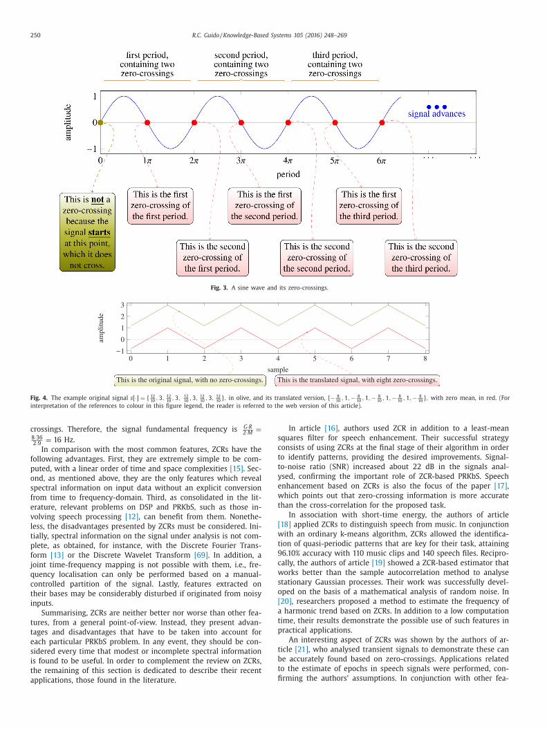
eriodic in 2 π , each period contains two zero-crossings, as shown
n Fig. 3 . Thus, if a 1D signal s [ ·] of length M crosses G times the
mplitude zero, it contains G 2 sinusoidal periods at that frequency.
onsidering that, at the time the signal was converted from its
nalog to its digital version [14] , the sampling rate was R sam-
les per second, then
1 R is the period of time between consecutive
amples, entailing that M · 1 R =
M
R is the time extension of the ana-
og signal in seconds. Concluding, in
M
R seconds there are G 2 sinu-
oidal periods, implying that, proportionally, there are G ·R 2 ·M
periods
er second, i.e., the frequency, F , caught by the ZCRs is
(ZCR ( f [ ·])) =
G · R
2 · M
Hz. (2)
Obviously, the previous formulation is only valid if the sinu-
oids are not shifted on the amplitude axis, i.e., no constant value
s added to them. Equivalently, the signal under analysis is required
o have its arithmetic mean equal zero, implying that an initial ad-
ustment may be necessary prior to counting the ZCRs, otherwise
hey would not be physically meaningful. The simplest process to
ormalise a signal s [ ·] in order to turn its mean to zero is to shift
ach one of its samples, subtracting its original mean, i.e.,
k ← s k −(∑ M−1
j=0 s j )
M
, (0 � k � M − 1) . (3)
In order to illustrate the concepts I have just exposed, the
eaders are requested to consider the signal s [ ·] = { 12 10 , 3 ,
12 10 , 3 ,
12 10 , 3 ,
12 10 , 3 ,
12 10 } , of length M = 9 , that was sampled at 36 sam-
les per second and is illustrated in Fig. 4 . Its arithmetic mean
s 12 10
+3+ 12 10
+3+ 12 10
+3+ 12 10
+3+ 12 10
9 = 2 � = 0 , i.e., the normalisation de-
ned in Eq. (3) must be applied before the ZCRs are counted.
hus, s [ ·] becomes { 12 10 − 2 , 3 − 2 , 12
10 − 2 , 3 − 2 , 12 10 − 2 , 3 − 2 , 12
10 − , 3 − 2 , 12
10 − 2 } = {− 8 10 , 1 , − 8
10 , 1 , − 8 10 , 1 , − 8
10 , 1 , − 8 10 } , which has
ts mean equal zero and is also shown in Fig. 4 . ZCRs are now
eady to be counted, according to Eq. (1) , resulting in G = 8 zero-
250 R.C. Guido / Knowledge-Based Systems 105 (2016) 248–269
Fig. 3. A sine wave and its zero-crossings.
Fig. 4. The example original signal s [ ·] = { 12 10
, 3 , 12 10
, 3 , 12 10
, 3 , 12 10
, 3 , 12 10
} , in olive, and its translated version, {− 8 10
, 1 , − 8 10
, 1 , − 8 10
, 1 , − 8 10
, 1 , − 8 10
} , with zero mean, in red. (For
interpretation of the references to colour in this figure legend, the reader is referred to the web version of this article).
s
c
t
t
y
e
w
t
[
w
t
9
c
w
s
o
[
a
t
p
t
b
t
fi
crossings. Therefore, the signal fundamental frequency is G ·R 2 ·M
=8 ·36 2 ·9 = 16 Hz.
In comparison with the most common features, ZCRs have the
following advantages. First, they are extremely simple to be com-
puted, with a linear order of time and space complexities [15] . Sec-
ond, as mentioned above, they are the only features which reveal
spectral information on input data without an explicit conversion
from time to frequency-domain. Third, as consolidated in the lit-
erature, relevant problems on DSP and PRKbS, such as those in-
volving speech processing [12] , can benefit from them. Nonethe-
less, the disadvantages presented by ZCRs must be considered. Ini-
tially, spectral information on the signal under analysis is not com-
plete, as obtained, for instance, with the Discrete Fourier Trans-
form [13] or the Discrete Wavelet Transform [69] . In addition, a
joint time-frequency mapping is not possible with them, i.e., fre-
quency localisation can only be performed based on a manual-
controlled partition of the signal. Lastly, features extracted on
their bases may be considerably disturbed if originated from noisy
inputs.
Summarising, ZCRs are neither better nor worse than other fea-
tures, from a general point-of-view. Instead, they present advan-
tages and disadvantages that have to be taken into account for
each particular PRKbS problem. In any event, they should be con-
sidered every time that modest or incomplete spectral information
is found to be useful. In order to complement the review on ZCRs,
the remaining of this section is dedicated to describe their recent
applications, those found in the literature.
In article [16] , authors used ZCR in addition to a least-mean
quares filter for speech enhancement. Their successful strategy
onsists of using ZCRs at the final stage of their algorithm in order
o identify patterns, providing the desired improvements. Signal-
o-noise ratio (SNR) increased about 22 dB in the signals anal-
sed, confirming the important role of ZCR-based PRKbS. Speech
nhancement based on ZCRs is also the focus of the paper [17] ,
hich points out that zero-crossing information is more accurate
han the cross-correlation for the proposed task.
In association with short-time energy, the authors of article
18] applied ZCRs to distinguish speech from music. In conjunction
ith an ordinary k-means algorithm, ZCRs allowed the identifica-
ion of quasi-periodic patterns that are key for their task, attaining
6.10% accuracy with 110 music clips and 140 speech files. Recipro-
ally, the authors of article [19] showed a ZCR-based estimator that
orks better than the sample autocorrelation method to analyse
tationary Gaussian processes. Their work was successfully devel-
ped on the basis of a mathematical analysis of random noise. In
20] , researchers proposed a method to estimate the frequency of
harmonic trend based on ZCRs. In addition to a low computation
ime, their results demonstrate the possible use of such features in
ractical applications.
An interesting aspect of ZCRs was shown by the authors of ar-
icle [21] , who analysed transient signals to demonstrate these can
e accurately found based on zero-crossings. Applications related
o the estimate of epochs in speech signals were performed, con-
rming the authors’ assumptions. In conjunction with other fea-

R.C. Guido / Knowledge-Based Systems 105 (2016) 248–269 251
Fig. 5. 1D example for B 1 aiming DSP and PRKbS with its variants TA, PA and EA: sliding window with length L = 8 traversing s [ ·] with overlap V = 50% . The symbols w i
represent the k th positioning of the window, for k = 0 , 1 , 2 , ..., T − 1 , and w h is the window that contains the highest number of ZCRs.
t
m
s
m
i
[
s
s
1
n
s
t
G
e
m
n
p
c
v
t
[
e
i
i
e
y
a
h
i
t
a
c
2
o
T
2
t
c
i
t
E
t
e
s
m
c
c
p
T
f
p
t
a
l
m
t
t
t
P
m
t
i
c
P
s
f
b
e
i
t
W
t
ures, such as energy, the authors of paper [22] present different
ethods to distinguish voiced from unvoiced segments in speech
ignals. Empirically, the size of the speech segments were deter-
ined for better accuracy during their successful analyses. Sim-
lar experiments were also performed by the authors of paper
23] , confirming the findings. In [24] , a practical and noise-robust
peech recognition system based on ZCRs was developed. Authors
howed improvements on baseline approaches at a rate of about
8.8%. Humanoid robots also benefit from ZCRs, for speech recog-
ition and segregation purposes, according to the experiments de-
cribed in [25] .
In order to successfully predict epileptic seizures in scalp elec-
roencephalogram signals, the authors of paper [26] modeled a
aussian Mixture of ZCRs intervals of occurrence, obtaining rel-
vant results. Interestingly, the authors of the paper [27] used a
odified ZCR to determine fractal dimensions of biomedical sig-
als. Similarly, in paper [28] , authors evaluate a modified ZCR ap-
roach for the detection of heart arrhythmias. A prominent appli-
ation of ZCRs can be found in paper [29] , in which authors de-
eloped a brain-computer interface on their basis. A health moni-
oring scheme based on ZCRs characterises the work described in
30] , for which interesting aspects of such features are pointed out.
Not surprisingly, a wide search on Web of Science and other sci-
ntific databases, aiming to find possible research articles describ-
ng applications of ZCRs on image processing and computer vision,
.e., 2D signals, returned a modest number of results: two confer-
nce papers, being one recent [31] and the other published twenty
ears ago [32] , and one journal paper published almost thirty years
go [33] . Possibly, this is due to the fact that digital images usually
ave their pixels represented as being positive integer numbers,
nhibiting the use of zero-crossings. In this study, in addition to
he novel ZCR-based algorithms designed for 1D signals, 2D ones
re also considered just after a proper pre-processing strategy dis-
ussed herein.
. The proposed methods
Three different methods, i.e., B 1 , B 2 and B 3 , respectively inspired
n A 1 , A 2 and A 3 introduced in [1] , are proposed in this section.
heir corresponding details follow.
.1. Method B 1
B 1 , illustrated in Fig. 5 , is the simplest method I present in
his study, in which an 1D discrete-time signal s [ ·] of length M is
onsidered as being the input. The procedure consists of a slid-
ng rectangular window, w , of length L traversing the signal so
hat, for each placement, the ZCR over that position is determined.
ach subsequent positioning overlaps in V % the previous one, being
he surplus samples at the end of the signal, which are not long
nough to be overlapped by a L -sample window, disposed. The re-
trictions (2 � L � M ) and (0 � V < 100) are mandatory.
In a DSP context, the ZCRs computed over the fragments of s [ ·]ay be directly used to determine the fundamental frequencies it
ontains, based on Eq. 2 . On the other hand, in case PRKbS asso-
iated with handcrafted FE is the objective, as explained in [1] -
p.2, s [ ·] requires its conversion to a feature vector, f [ ·], of length
= � (100 ·M) −(L ·V ) (100 −V ) ·L � , being � · � the floor operator. In this case, each
k , (0 � k � T − 1) , corresponds to the ZCR computed over the k th
osition of the window w . Of fundamental importance is the fact
hat, for handcrafted FE, f [ ·] requires normalisation prior to its use
s an input for a classifier, as documented in [1] -pp.2.
There are, basically, three possible ways to normalise f [ ·]: in re-
ation to the total amount (TA) of zero-crossings, in relation to the
aximum possible amount (PA) of zero-crossings and in relation
o the maximum existing amount (EA) of zero-crossings. Each of
he normalisations characterises a particular physical meaning for
he ZCRs contained in f [ ·], being adequate for a specific task in
RKbS. Comments on each of them follow, nonetheless, all the nor-
alisations force f [ ·] to express a rate , bringing the proper sense to
he letter “R” used in the abbreviation “ZCR”.
The division of each individual ZCR in f [ ·] by the sum of all ZCRs
t contains, i.e.,
f r ←
f r (∑ T −1 k =0 f k
) , (0 � r � T − 1) ,
haracterises TA. Once this procedure is adopted, ∑ T −1
k =0 f k = 1 .
hysically, TA forces f [ ·] to express the fraction of ZCRs in each
egment of s [ ·], being ideal to describe the way the fundamental
requencies of an input signal, s [ ·], vary in relation to its overall
ehaviour.
To force f [ ·] express individual spectral properties related to
ach fragment of s [ ·], in isolation, PA is required. The correspond-
ng normalisation consists of dividing each ZCR in f [ ·] by L − 1 , i.e.,
he highest possible number of ZCRs inside a window of length L :
f r ←
f r
L − 1
, (0 � r � T − 1) .
ith this procedure, f k ≤ 1, for (0 � k � T − 1) . The closer a cer-
ain f is to 0 or to 1, respectively, the lowest or highest the fun-
k
252 R.C. Guido / Knowledge-Based Systems 105 (2016) 248–269
Algorithm 1 : fragment of C++ code for method B 1 in 1D, adopting
the normalisation TA. //...
// ensure that s [ ·] , of length M, is available as input
double mean = 0 ;
for(int k = 0 ; k < M; k + + )
mean + = s [ k ] / (double )(M) ;
for(int k = 0 ; k < M; k + + )
s [ k ] − = mean ; // at this point, the arithmetic mean of the input signal is 0
int L = / * the desired positive value, not higher than M * / ;
int V = / * the desired positive value, lower than 100 * / ;
int T = (int)(( 100 ∗ M − L ∗ V )/(( 100 − V ) ∗L ));
int ZCR = 0 ; // ZCR is the total number of zero-crossings over all the window place-
ments, required for normalisation
double ∗ f = new double[ T ]; // dynamic vector declaration
for(int k = 0 ; k < T ; k + + )
{
f [ k ] = 0 ;
for(int i = k ∗ ((int )(((100 − V ) / 100 . 0) ∗ L )) ; i < k ∗ ((int )(((100 −V ) / 100 . 0) ∗ L )) + L − 1 ; i + + )
f [ k ]+ = ( s [ i ] ∗ s [ i + 1] < 0 )?1:0; / ∗ multiplying subsequent samples
results in a negative value if they are between 0. This is equivalent to the theoretical
procedure described in the text and based on equation 1. ∗/
ZCR + = f [ k ] ;
}
for(int k = 0 ; k < T ; k + + ) // normalisation
f [ k ] / = (double )(ZCR ) ; / ∗ the casting, i.e., the explicit conversion of ZCR
from int to double is, theoretically, not required, however, some C/C++ compilers have
presented problems when a double-precision variable is divided by an int one, result-
ing in 0. To avoid this issue, the casting is used. ∗/
// at this point, the feature vector, f [ ·] , is ready
//...
Algorithm 2 : fragment of C++ code for method B 1 in 1D, adopting
the normalisation PA. //...
// ensure that s [ ·] , of length M, is available as input
double mean = 0 ;
for(int k = 0 ; k < M; k + + )
mean + = s [ k ] / (double )(M) ;
for(int k = 0 ; k < M; k + + )
s [ k ] − = mean ; // at this point, the arithmetic mean of the input signal is 0
int L = / * the desired positive value, not higher than M * / ;
int V = / * the desired positive value, lower than 100 * / ;
int T = (int)(( 100 ∗ M − L ∗ V )/(( 100 − V ) ∗L ));
double ∗ f = new double[ T ]; // dynamic vector declaration
for(int k = 0 ; k < T ; k + + )
{
f [ k ] = 0 ;
for(int i = k ∗ ((int )(((100 − V ) / 100 . 0) ∗ L )) ; i < k ∗ ((int )(((100 −V ) / 100 . 0) ∗ L )) + L − 1 ; i + + )
f [ k ]+ = ( s [ i ] ∗ s [ i + 1] < 0 )?1:0; / ∗ multiplying subsequent samples
results in a negative value if they are between 0. This is equivalent to the theoretical
procedure described in the text and based on equation 1. ∗/
f [ k ] / = (double )(L − 1) ; / ∗ the casting, i.e., the explicit conversion of L from
int to double is, theoretically, not required, however, some C/C++ compilers have pre-
sented problems when a double-precision variable is divided by an int one, resulting
in 0. To avoid this issue, the casting is used. ∗/
}
// at this point, the feature vector, f [ ·] , is ready
//...
2
s
l
v
t
m
i
i
damental frequency at the corresponding window is, disregarding
the remaining fragments of s [ ·]. Lastly, EA is chosen whenever evaluation by comparison is
needed, particularly forcing the highest ZCR in f [ ·] to be 1 and ad-
justing the remaining ones, proportionally, within the range (0 −1) .
The corresponding procedure consists of dividing each individual
ZCR in f [ ·] by the highest unnormalised ZCR contained in it, the
one computed over the window placement named w h , i.e.,
f r ←
f r
ZCR (w h ) , (0 � r � T − 1) .
All the previous formulations and concepts can be easily ex-
tended to a 2D signal, m [ ·][ ·], with N rows and M columns, which
represent, respectively, the height and width of the corresponding
image. As in the unidimensional case, the computation of a bidi-
mensional ZCR requires all the values in m [ ·][ ·] to be previously
shifted so that its arithmetic mean becomes equal zero, i.e.,
m p,q ← m p,q −(∑ N−1
i =0
∑ M−1 j=0 m i, j
)M · N
,
(0 � p � M − 1) , (0 � q � N − 1) . (4)
Once m [ ·][ ·] presents zero mean, its ZCR is simply the sum of
individual ZCRs in each row and column, i.e.,
ZCR (m [ ·][ ·]) =
1
2
N−1 ∑
i =0
M−2 ∑
j=0
| sign (m i, j ) − sign (m i, j+1 ) |
+
1
2
M−1 ∑
j=0
N−2 ∑
i =0
| sign (m i, j ) − sign (m i +1 , j ) | . (5)
Similarly to 1D signals, ZCRs computed in 2D are useful for both
DSP and FE in PRKbS, as illustrated in Fig. 6 . In the latter, the case
of interest, the feature vector, f [ ·], contains not only T , but T · P
elements, being P = � (100 ·N) −(L ·V ) (100 −V ) ·L � , as in the bidimensional case of
method A 1 , explained in [1] -pp.3. During the analysis, m [ ·][ ·] is tra-
versed along the horizontal orientation based on T placements of
the square window w of side L , being L < M and L < N . Then, the
process is repeated for each one of the P shifts along the vertical
orientation.
TA, PA and EA are also the possible normalisations for the 2D
version of B 1 applied for FE in PRKbS. Particularly, TA requires each
component of f [ ·] to be divided by the sum of all ZCRs it contains,
i.e., the sum of all the values in that vector prior to any normali-
sation. On the other hand, if PA is adopted, each element in f [ ·] isdivided by the maximum possible number of ZCRs inside w , i.e.,
(L − 1) ︸ ︷︷ ︸ maximum ZCR
in one row
· (L ) ︸︷︷︸ number of
rows
+ (L − 1) ︸ ︷︷ ︸ maximum ZCR
in one column
· (L ) ︸︷︷︸ number of
columns
= 2 · L · (L − 1) .
Lastly, the choice for EA implies that each component of f [ ·] is di-
vided by the highest ZCR contained in it, the one computed over
the window placement named w h .
Exactly as in A 1 [1] , for both 1D and 2D signals, respectively,
B 1 is only capable of generating a T , or a T · P , sample-long vec-
tor f [ ·] if the value of L is subjected to the value of M , or M
and N . Thus, the value of L intrinsically depends on the length of
the input 1D signal s [ ·], or the dimensions of the input 2D ma-
trix m [ ·][ ·], bringing a disadvantage: irregular, temporal or spatial
analysis. Oppositely, the advantage is that a few sequential ele-
ments of f [ ·], obtained by predefining L, T and P , allow the de-
tection of some particular event in the 1D or 2D signal under
analysis.
The algorithms 1 , 2 and 3 , respectively, contain the source code
in C/C++ programming language that implement method B 1 with
the normalisations TA, PA and EA, all of them for 1D input signals.
At variance with this, algorithms 4 , 5 and 6 correspond, respec-
tively, to the 2D versions of B with the same normalisations.
1.2. Method B 2
B 2 , as A 2 in [1] , is also based on a sliding window w traversing
[ ·], or m [ ·][ ·]. Two differences, however, exist: there are no over-
aps and the window length for 1D, or the rectangle sizes for 2D,
ary. Thus, s [ ·] or m [ ·][ ·] are inspected in different levels of resolu-
ion.
After applying Eq. (3) or Eq. ( 4 ), respectively to remove the
ean of s [ ·] or of m [ ·][ ·], the feature vector, f [ ·], is defined as be-
ng the concatenation of Q sub-vectors of different dimensions, i.e.,
f [ ·] = { ξ1 [ ·] } ∪ { ξ2 [ ·] } ∪ { ξ3 [ ·] } ∪ ... ∪ { ξQ [ ·] } . For 1D, each sub-vector
s created by placing w over T non-overlapping sequential positions

R.C. Guido / Knowledge-Based Systems 105 (2016) 248–269 253
Fig. 6. 2D example for B 1 aiming DSP and PRKbS with its variants TA, PA and EA: sliding square with length L = 3 traversing m [ ·][ ·] with overlap V = 66 . 67% . Again, w k [ · ]
indicate the k th position of the window, for k = 0 , 1 , 2 , ..., (T · P) − 1 . Dashed squares in the arbitrary positions 0, 1, 15, 16, 41 and 63, are shown.
o
E
l
e
v
f
w
t
p
i
i
e
z
e(︸
f s [ ·] and then calculating the normalised ZCRs using TA, PA, or
A, as previously explained during the description of B 1 , i.e.,:
• subvector ξ 1 [ ·] is obtained by letting L = � M
2 � and V = 0% ,
which that T = � (100 ·M) −(L ·V ) (100 −V ) ·L � = 2 , to traverse s [ ·] and get the
normalised ZCRs;
• idem to subvector ξ 2 [ ·], obtained by letting L = � M
3 � and V =0% , which that T = � (100 ·M) −(L ·V )
(100 −V ) ·L � = 3 ;
• idem to subvector ξ 3 [ ·], obtained by letting L = � M
5 � and V =0% , which that T = � (100 ·M) −(L ·V )
(100 −V ) ·L � = 5 ;
• . . .
• idem to subvector ξQ [ ·], obtained by letting L = � M
X � and V =0% , which that T = � (100 ·M) −(L ·V )
(100 −V ) ·L � = X .
Q is defined on the basis of the desired refinement and, simi-
arly, the values 2, 3, 5, 7, 9, 11, 13, 17, ..., X are choices for T , that is
ssentially restricted to prime numbers in order to avoid one sub-
ector to be a linear combination of another, implying in no gain
or classification.
For the 2D case, each sub-vector is created by framing m [ ·][ ·]ith T · P non-overlapping rectangles, being T = P prime numbers,
o compute the corresponding normalised ZCRs, i.e.,
• subvector ξ 1 [ ·] is created by letting L = � M
2 � and V = 0% to
obtain T = � (100 ·M) −(L ·V ) (100 −V ) ·L � = 2 and then by letting L = � N 2 � and
V = 0% to obtain P = � (100 ·N) −(L ·V ) (100 −V ) ·L � = 2 . Subsequently, m [ ·][ ·] is
traversed by T · P = 2 · 2 = 4 non-overlapping rectangles ;
• idem to subvector ξ 2 [ ·], obtained by letting L = � M
3 � and
V = 0% and then L = � N � and V = 0% , which that T =
3� (100 ·M) −(L ·V ) (100 −V ) ·L � = 3 and P = � (100 ·N) −(L ·V )
(100 −V ) ·L � = 3 , respectively, im-
plying that T · P = 3 · 3 = 9 non-overlapping rectangles traverse
m [ ·][ ·]; • idem to subvector ξ 3 [ ·], obtained by letting L = � M
5 � and
V = 0% and then L = � N 5 � and V = 0% , which that T =� (100 ·M) −(L ·V )
(100 −V ) ·L � = 5 and P = � (100 ·N) −(L ·V ) (100 −V ) ·L � = 5 , respectively, im-
plying that T · P = 5 · 5 = 25 non-overlapping rectangles tra-
verse m [ ·][ ·]; • . . .
• idem to subvector ξQ [ ·], obtained by letting L = � M
X � and
V = 0% and then L = � N X � and V = 0% , which that T =� (100 ·M) −(L ·V )
(100 −V ) ·L � = X and P = � (100 ·N) −(L ·V ) (100 −V ) ·L � = X, respectively, im-
plying that T · P = X · X = X 2 non-overlapping rectangles tra-
verse m [ ·][ ·];
In the 2D version of B 2 , the normalisations TA and EA are im-
lemented exactly as they were in B 1 . One particular note regard-
ng the normalisation PA is, however, important. Differently to B 1 n 2D, in which L is the same for both horizontal and vertical ori-
ntations, B 2 divides the input image into rectangles, i.e., the hori-
ontal and vertical sides are � M
X � and � N X � , respectively. Thus, each
lement of f [ ·] is not divided by 2 · L · (L − 1) , but by
� M
X
� − 1
) ︷︷ ︸
maximum ZCR
in one row
· � N
X
� ︸︷︷︸ number of
rows
+
(� N
X
� − 1
)︸ ︷︷ ︸
maximum ZCR
in one column
· � M
X
� ︸ ︷︷ ︸ number of
columns
= 2 · � M � · � N � − � M � − � N � ,
X X X X
254 R.C. Guido / Knowledge-Based Systems 105 (2016) 248–269
Algorithm 3 : fragment of C++ code for method B 1 in 1D, adopting
the normalisation EA. // ensure that s [ ·] , of length M, is available as input
double mean = 0 ;
for(int k = 0 ; k < M; k + + )
mean + = s [ k ] / (double )(M) ;
for(int k = 0 ; k < M; k + + )
s [ k ] − = mean ; // at this point, the arithmetic mean of the input signal is 0
int L = / * the desired positive value, not higher than M * / ;
int V = / * the desired positive value, lower than 100 * / ;
int T = (int)(( 100 ∗ M − L ∗ V )/(( 100 − V ) ∗L ));
int highest _ ZCR = 0 ;
double ∗ f = new double[ T ]; // dynamic vector declaration
for(int k = 0 ; k < T ; k + + )
{
f [ k ] = 0 ;
for(int i = k ∗ ((int )(((100 − V ) / 100 . 0) ∗ L )) ; i < k ∗ ((int )(((100 −V ) / 100 . 0) ∗ L )) + L − 1 ; i + + )
f [ k ]+ = ( s [ i ] ∗ s [ i + 1] < 0 )?1:0; / ∗ multiplying subsequent samples
results in a negative value if they are between 0. This is equivalent to the theoretical
procedure described in the text and based on equation 1. ∗/
if ( f [ k ] > highest _ ZCR )
highest _ ZCR = f [ k ] ;
}
for(int k = 0 ; k < T ; k + + )
f [ k ] / = (double )(highest _ ZCR ); / ∗ the casting, i.e., the explicit conversion of
highest_ZCR from int to double is, theoretically, not required, however, some C/C++
compilers have presented problems when a double-precision variable is divided by
an int one, resulting in 0. To avoid this issue, the casting is used. ∗/
// at this point, the feature vector, f [ ·] , is ready
Algorithm 4 : fragment of C++ code for method B 1 in 2D, adopting
the normalisation TA. // ensure that m [ ·][ ·] , with height N and width M, is available as input
double mean = 0 ;
for(int p = 0 ; p < N; p + + )
for(int q = 0 ; q < M; q + + )
mean + = m [ p][ q ] / (double )(M ∗ N) ;
for(int p = 0 ; p < N; p + + )
for(int q = 0 ; q < M; q + + )
m [ p][ q ] − = mean ; // at this point, the arithmetic mean of the input
signal is 0
int L = / * the desired positive value, not higher than the higher between M and N
* / ;
int V = / * the desired positive value, lower than 100 * / ;
int T = (int)(( 100 ∗ M − L ∗ V )/(( 100 − V ) ∗L ));
int P = (int)(( 100 ∗ N − L ∗ V )/(( 100 − V ) ∗L ));
int ZCR = 0 ; // ZCR is the total number of zero-crossings over all the window place-
ments, required for normalisation
double ∗ f = new double[ T ∗ P]; // dynamic vector declaration
for(int k = 0 ; k < T ∗ P; k + + )
{
f [ k ] = 0 ;
for(int i = k ∗ ((int )(((100 − V ) / 100 . 0) ∗ L )) ; i < k ∗ ((int )(((100 −V ) / 100 . 0) ∗ L )) + L ; i + + )
for(int j = k ∗ ((int )(((100 − V ) / 100 . 0)) ∗ L ) ; j < k ∗ ((int )(((100 −V ) / 100 . 0)) ∗ L ) + L − 1 ; j + + )
f [ k ]+ = ( m [ i ][ j] ∗ m [ i ][ j + 1] < 0 )?1:0; / ∗ multiplying sub-
sequent samples results in a negative value if they are between 0. This is equivalent
to the theoretical procedure described in the text and based on equation 1. ∗/
for(int i = k ∗ ((int )(((100 − V ) / 100 . 0) ∗ L )) ; i < k ∗ ((int )(((100 −V ) / 100 . 0) ∗ L )) + L − 1 ; i + + )
for(int j = k ∗ ((int )(((100 − V ) / 100 . 0)) ∗ L ) ; j < k ∗ ((int )(((100 −V ) / 100 . 0)) ∗ L ) + L ; j + + )
f [ k ]+ = ( m [ i ][ j] ∗ m [ i + 1][ j] < 0 )?1:0; / ∗ multiplying sub-
sequent samples results in a negative value if they are between 0. This is equivalent
to the theoretical procedure described in the text and based on equation 1. ∗/
ZCR + = f [ k ] ;
}
for(int k = 0 ; k < T ∗ P; k + + )
f [ k ] / = (double )(ZCR ) ; / ∗ the casting, i.e., the explicit conversion of ZCR
from int to double is, theoretically, not required, however, some C/C++ compilers have
presented problems when a double-precision variable is divided by an int one, result-
ing in 0. To avoid this issue, the casting is used. ∗/
// at this point, the feature vector, f [ ·] , is ready
Algorithm 5 : fragment of C++ code for method B 1 in 2D, adopting
the normalisation PA.
// ensure that m [ ·][ ·] , with height N and width M, is available as inputdouble mean = 0 ; for(int p = 0 ; p < N; p + + )
for(int q = 0 ; q < M; q + + ) mean + = m [ p][ q ] / (double )(M ∗ N) ;
for(int p = 0 ; p < N; p + + ) for(int q = 0 ; q < M; q + + )
m [ p][ q ] − = mean ; // at this point, the arithmetic mean of the input signal is 0 int L = / * the desired positive value, not higher than the higher between M
and N * / ; int V = / * the desired positive value, lower than 100 * / ; int T = (int)(( 100 ∗ M − L ∗ V )/(( 100 − V ) ∗L )); int P = (int)(( 100 ∗ N − L ∗ V )/(( 100 − V ) ∗L )); double ∗ f = new double[ T ∗ P]; // dynamic vector declaration for(int k = 0 ; k < T ∗ P; k + + )
{ f [ k ] = 0 ; for(int i = k ∗ ((int )(((100 − V ) / 100 . 0) ∗ L )) ; i < k ∗ ((int )(((100 −
V ) / 100 . 0) ∗ L )) + L ; i + + ) for(int j = k ∗ ((int )(((100 − V ) / 100 . 0)) ∗ L ) ; j <
k ∗ ((int )(((100 − V ) / 100 . 0)) ∗ L ) + L − 1 ; j + + ) f [ k ]+ = ( m [ i ][ j] ∗ m [ i ][ j + 1] < 0 )?1:0; / ∗ multiplying
subsequent samples results in a negative value if they are between 0. This is equivalent to the theoretical procedure described in the text and based on equation 1. ∗/
for(int i = k ∗ ((int )(((100 − V ) / 100 . 0) ∗ L )) ; i < k ∗ ((int )(((100 −V ) / 100 . 0) ∗ L )) + L − 1 ; i + + )
for(int j = k ∗ ((int )(((100 − V ) / 100 . 0)) ∗ L ) ; j <
k ∗ ((int )(((100 − V ) / 100 . 0)) ∗ L ) + L ; j + + ) f [ k ]+ = ( m [ i ][ j] ∗ m [ i + 1][ j] < 0 )?1:0; / ∗ multiplying
subsequent samples results in a negative value if they are between 0. This is equivalent to the theoretical procedure described in the text and based on equation 1. ∗/
} for(int k = 0 ; k < T ∗ P; k + + )
f [ k ] / = (double )(2 ∗ L ∗ (L − 1)) ; the casting, i.e., the explicit conver- sion of L from int to double is, theoretically, not required, however, some C/C++ compilers have presented problems when a double-precision variable is divided by an int one, resulting in 0. To avoid this issue, the casting is used. ∗/
// at this point, the feature vector, f [ ·] , is ready
t
c
r
a
t
2
o
s
o
d
t
c
i
r
(
d
hat corresponds to the maximum possible number of zero-
rossings in each rectangular sub-image.
Figs. 7 and 8 show the sliding window for 1D and the sliding
ectangle for 2D, respectively, for TA , PA and EA . In addition, the
lgorithms 8 , 7 and 9 contain the corresponding 1D implementa-
ions. The 2D ones are in the algorithms 10–12 .
.3. Method B 3
As described above, B 1 and B 2 focus on measuring the levels
f normalised ZCRs over windows or rectangles of certain dimen-
ions. B 3 , on the other hand, is quite similar to A 3 [1] and consists
f determining the proportional lengths, or areas, of the signal un-
er analysis that are required to reach predefined percentages of
he total ZCR. Normalisations do not apply in this case. The direct
onsequence of this approach is the characterisation of B 3 as being
deal to inspect the constancy in frequency of the physical entity
esponsible for generating s [ ·], or m [ ·][ ·]. Specifically, C is defined as being the critical base-level of ZCRs,
0 < C < 100), and then, for 1D, the feature vector f [ ·] of size T is
etermined as follows:
• f 0 is the proportion of the length of s [ ·], i.e., M , starting from its
beginning, which is covered by the window placement w 0 [ · ],
required to reach C % of the total ZCR;
• f B is the proportion of the length of s [ ·], i.e., M , starting from its
beginning, which is covered by the window placement w 1 [ · ],
required to reach 2 · C % of the total ZCR;

R.C. Guido / Knowledge-Based Systems 105 (2016) 248–269 255
Fig. 7. 1D example for B 2 assuming Q = 3 : (a) sliding window, with length L = � M 2 � = � 20
2 � = 10 traversing s [ ·] in order to compose ξ 1 [ ·]; (b) sliding window with length
L = � M 3 � = � 20
3 � = 6 traversing s [ ·] in order to compose ξ 2 [ ·]; (c) sliding window with length L = � M
5 � = � 20
5 � = 4 traversing s [ ·] in order to compose ξ 3 [ ·]. The window
positions do not overlap and the symbols w i indicate the i th window position, for i = 0 , 1 , 2 , ..., T − 1 .
T
T
t
i
1 I will take this opportunity to correct an error in my previous published tutorial
[1] -pp.270 regarding the description of A 3 in 2D: the way αi and β i vary is in ac-
cordance with a relationship between N and M , as shown above, instead of αi and
• f A is the proportion of the length of s [ ·], i.e., M , starting from its
beginning, which is covered by the window placement w 2 [ · ],
required to reach 3 · C % of the total ZCR;
• . . .
• f T −1 is the proportion of the length of s [ ·], i.e., M , starting
from its beginning, which is covered by the window placement
w T −1 [ ·] , required to reach ( T · C )% of the total ZCR, so that ( T ·C ) < 100%;
For B 3 , the value of T is defined as being:
=
{100
C − 1 if C is multiple of 100 ;
� 100 C
� otherwise .
he 2D version of B 3 implies that f [ ·], with the same size T , is de-
ermined as follows:
• f 0 is the proportion of m [ ·][ ·] area, i.e., M · N , starting from m 0, 0
and covered by the � α0 � x � β0 � rectangle w 0 [ · ][ · ], required
to reach C % of the total ZCR;
• f B is the proportion of m [ ·][ ·] area, i.e., M · N , starting from m 0, 0
and covered by the � α1 � x � β1 � rectangle w 1 [ · ][ · ], required
to reach 2 · C % of the total ZCR;
• f A is the proportion of m [ ·][ ·] area, i.e., M · N , starting from m 0, 0
and covered by the � α2 � x � β2 � rectangle w 2 [ · ][ · ], required
to reach 3 · C % of the total ZCR;
• . . .
• f T P−1 is the proportion of m [ ·][ ·] area, i.e., M · N , starting from
m 0, 0 and covered by the � αT −1 � x � βT −1 � rectangle w T −1 [ ·][ ·] ,required to reach T · C % of the total ZCR, so that ( T · C ) < 100%;
The values of αi and β i , ( 0 � i � T − 1 ), are determined accord-
ng to the following rule, the exact same used for A 3 in 2D
1 [1] :

256 R.C. Guido / Knowledge-Based Systems 105 (2016) 248–269
Fig. 8. 2D example for B 2 assuming Q = 3 subvectors: [above] sliding square with length {� M 2 � x � N
2 �} = {� 10
2 � x � 20
2 �} = 5 x 10 traversing m [ ·][ ·] in order to compose ξ 1 [ ·]; [mid-
dle] sliding square with length {� M 3 � x � N
3 �} = {� 10
3 � x � 20
3 �} = 3 x 6 traversing m [ ·][ ·] in order to compose ξ 2 [ ·]; [below] sliding square with length {� M
5 � x � N
5 �} = {� 10
5 � x � 20
5 �} =
2 x 4 traversing m [ ·][ ·] in order to compose ξ 3 [ ·]. Again, w i indicates the i th window position, for i = 0 , 1 , 2 , ..., (T · P) − 1 , with no overlap. Dashed squares represent the sliding
window in all possible positions.
e
2
e
Beginning: (αi ← 0) and (βi ← 0) , unconditionally .
repeat
{
(αi ← αi + 1) and (βi ← βi + 1) if (N = M)
(αi ← αi + 1) and (βi ← βi +
M
N ) if (N > M)
(αi ← αi +
N M
) and (βi ← βi + 1) otherwise .
until the desired level of energy, i.e., C , 2 · C , 3 · C , ..., T · C is
reached.
β i themselves, as originally documented in that paper. A corrigendum is available
on-line at http://dx.doi.org/10.1016/j.neucom.2016.04.001 with details.
s
g
End. Figs. 9 and 10 , and algorithms 13 and 14 2 , complement my
xplanations regarding B 3 , for both 1D and 2D, respectively.
.4. ZCRs are neurocomputing agents
In this subsection, the trail for an interesting point-of-view is
xplained. Additionally to Eq. 1 , ZCRs may also be counted based
2 The algorithm for A 3 in 2D, originally described in [1] -pp.273, also requires the
ame corrections I mentioned in the previous footnote, as described in the corri-
endum.

R.C. Guido / Knowledge-Based Systems 105 (2016) 248–269 257
Fig. 9. 1D example for B 3 , where L w i represents the length of the window w i [ · ], for i = 0 , 1 , 2 , 3 , ..., T − 1 .
Fig. 10. 2D example for B 3 , where w i [ · ] corresponds to the i th window, and αi and β i represent, respectively, its height and width, for i = 0 , 1 , 2 , 3 , ..., T P − 1 .
Fig. 11. The sigmoide function, y =
1 1+ e −γ ·x , exemplified for different values of γ :
2, 5 and 10 0 0, respectively drawn in green, blue and brown. The proposed strategy
requires γ >> 0 aiming at a response as the one drawn in brown.(For interpretation
of the references to colour in this figure legend, the reader is referred to the web
version of this article).
o
t
c
1 ,
b
−
p
f
t
t
s
t
h
b
Z
i
t
d ∑
t
F
t
d
o
t
p
k
t
l
c
t
k
t
t
t
n
t
3
n
n a different strategy, which is the one I use in my algorithms:
wo adjacent samples of a discrete-time signal, lets say s i and s i +1 ,
ross zero whenever their product is negative. Thus,
s i · s i +1
| s i · s i +1 | =
{−1 if there is a zero-crossing between s i and s i +1 otherwise
eing the denominator used for normalisation.
Purposely, I am inverting the polarities hereafter so thats i ·s i +1 | s i ·s i +1 | becomes either 1 or −1 , respectively, in response to the
resence or absence of a zero-crossing. Furthermore, despite the
act that 1 | s i ·s i +1 | is the simplest existing normalisation, I am going
o replace it by a more convenient formulation to reach my objec-
ive: the sigmoide function parametrised with a slope γ > > 0, as
hown in Fig. 11 . We therefore have
1
1 + e −γ (−s i ·s i +1 ) =
{
1 if there is a zero-crossing between
s i and s i +1
0 otherwise .
In order to traverse a window of length L and count its ZCRs,
he summation
∑ L −2 i =0
1
1+ e −γ (−s i ·s i +1 ) is adopted. The readers may
ave learnt that, for FE, we are interested in the normalised num-
er of ZCRs instead of its raw amount. Thus,
CR (s [ ·]) =
1
β·
L −2 ∑
i =0
1
1 + e −γ (−s i ·s i +1 ) =
L −2 ∑
i =0
1
β· 1
1 + e −γ (−s i ·s i +1 )
s the simplest possibility to obtain a bounded outcome within
he range from 0 to 1. Particularly, TA, PA and EA can be ad-
ressed as a function of β , respectively, by letting it be equal to T −1 k =0
ZCR (w k [ ·]) , L − 1 and ZCR ( w h [ · ]), as I defined previously.
Clearly, the structure I propose corresponds to the original mul-
ilayer perceptron defined by Frank Rosenblatt [34] , as shown in
ig. 12 , with some peculiarities. Its i th input, i th weight between
he input and the hidden layers, and i th weight between the hid-
en and the output layers are, respectively, s i , −s i +1 and 1 β
. More-
ver, the i th neuron of the input layer connects forward only with
he i th of the hidden one. Another possible interpretation for the
roposed structure is that of a weightless neural network, also
nown as random access memory (RAM) network [35–37] , so that
here are weights albeit pre-defined, implying that there is no
earning procedure.
Concluding, when we are counting the normalised ZCRs of a
ertain signal, we are somehow neurocomputing it, moreover, on
he basis of neurons which were “born with a pre-established
nowledge”. The potential of ZCRs awakens deeper attraction upon
heir characterisation as being specific neurocomputing agents,
hus, my expectation is that the interdisciplinary community in-
erested in PRKbS, FE, computational intelligence, artificial neural
etworks, DSP and related fields will frequently take advantage of
he methods I present.
. Numerical examples
In order to shed some light on the proposed approaches, one
umerical example follows for each case: methods B , B and B ,
1 2 3
258 R.C. Guido / Knowledge-Based Systems 105 (2016) 248–269
Fig. 12. The proposed structure, with pre-defined weights.
Algorithm 6 : fragment of C++ code for method B 1 in 2D, adopting
the normalisation EA.
// ensure that m [ ·][ ·] , with height N and width M, is available as inputdouble mean = 0 ; for(int p = 0 ; p < N; p + + )
for(int q = 0 ; q < M; q + + ) mean + = m [ p][ q ] / (double )(M ∗ N) ;
for(int p = 0 ; p < N; p + + ) for(int q = 0 ; q < M; q + + )
m [ p][ q ] − = mean ; // at this point, the arithmetic mean of the input signal is 0 int L = / * the desired positive value, not higher than the higher between M
and N * / ; int V = / * the desired positive value, lower than 100 * / ; int T = (int)(( 100 ∗ M − L ∗ V )/(( 100 − V ) ∗L )); int P = (int)(( 100 ∗ N − L ∗ V )/(( 100 − V ) ∗L )); int highest _ ZCR = 0 ; // ZCR is the total number of zero-crossings over all the window placements, required for normalisation double ∗ f = new double[ T ∗ P]; // dynamic vector declaration for(int k = 0 ; k < T ∗ P; k + + )
{ f [ k ] = 0 ; for(int i = k ∗ ((int )(((100 − V ) / 100 . 0) ∗ L )) ; i < k ∗ ((int )(((100 −
V ) / 100 . 0) ∗ L )) + L ; i + + ) for(int j = k ∗ ((int )(((100 − V ) / 100 . 0)) ∗ L ) ; j <
k ∗ ((int )(((100 − V ) / 100 . 0)) ∗ L ) + L − 1 ; j + + ) f [ k ]+ = ( m [ i ][ j] ∗ m [ i ][ j + 1] < 0 )?1:0; / ∗ multiplying
subsequent samples results in a negative value if they are between 0. This is equivalent to the theoretical procedure described in the text and based on equation 1. ∗/
for(int i = k ∗ ((int )(((100 − V ) / 100 . 0) ∗ L )) ; i < k ∗ ((int )(((100 −V ) / 100 . 0) ∗ L )) + L − 1 ; i + + )
for(int j = k ∗ ((int )(((100 − V ) / 100 . 0)) ∗ L ) ; j <
k ∗ ((int )(((100 − V ) / 100 . 0)) ∗ L ) + L ; j + + ) f [ k ]+ = ( m [ i ][ j] ∗ m [ i + 1][ j] < 0 )?1:0; / ∗ multiplying
subsequent samples results in a negative value if they are between 0. This is equivalent to the theoretical procedure described in the text and based on equation 1. ∗/
if ( f [ k ] > highest _ ZCR ) highest _ ZCR = f [ k ] ;
} for(int k = 0 ; k < T ∗ P; k + + )
f [ k ] / = (double )(highest _ ZCR ) ; the casting, i.e., the explicit conver- sion of highest_ZCR from int to double is, theoretically, not required, however, some C/C++ compilers have presented problems when a double-precision vari- able is divided by an int one, resulting in 0. To avoid this issue, the casting is used. ∗/
// at this point, the feature vector, f [ ·] , is ready
V
Algorithm 7 : fragment of C++ code for method B 2 in 1D, adopting
the normalisation TA. // ensure that s [ ·] , of length M, is available as input
double mean = 0 ;
for(int k = 0 ; k < M; k + + )
mean + = s [ k ] / (double )(M) ;
for(int k = 0 ; k < M; k + + )
s [ k ] − = mean ; // at this point, the arithmetic mean of the input signal is 0
int L ; // window length
int ZCR ; // ZCR represents the total ZCR over all the window positions, that is re-
quired to normalise f [ ·] int X[] = { 2 , 3 , 5 , 7 , 9 , 11 , 13 , 17 } ; /* vector containing the prime numbers of interest.
It can be changed according to the experiment */
int total_size_of_f = 0 ;
for(int i = 0 ; i < (int)(sizeof( X)/sizeof(int)); i + + ) // number of elements in X[ ·] total_size_of_f+=X[i];
double ∗ f = new double[total_size_of_f]; /* The total size of f [ ·] is the sum of the
elements in X[ ·] , i.e., the size of the subvector ξ1 [ ·] plus the size of the subvector
ξ2 [ ·] , plus the size of the subvector ξ3 [ ·] , ..., and so on */
int jump = 0; // helps to control the correct positions to write in f [ ·] for(int j = 0 ; j < (int)(sizeof( X)/sizeof(int)) ; j + + )
{
ZCR = 0 ;
for(int k = 0 ; k < X[ j] ; k + + )
{
L = (int)(M/X[ j]) ;
f [ jump + k ] = 0 ;
for(int i = (k ∗ L ) ; i < (k ∗ L ) + L ; i + + )
f [ jump + k ]+ = ( s [ i ] ∗ s [ i + 1] < 0 )?1:0;
ZCR + = f [ jump + k ] ;
}
for(int k = 0 ; k < X[ j] ; k + + )
f [ jump + k ] / = (double )(ZCR ) ;
jump+ = X[ j] ;
}
// at this point, the feature vector, f [ ·] , is ready
v
i
b
{
i
1
e
i
{
both in 1D and 2D, assuming the normalisations previously de-
scribed and based on hypothetical data.
3.1. Numerical example for B 1 in 1D
Problem statement : Let s [ ·] = { 1 , 2 , 3 , 4 , 5 , 5 , 4 , 3 , 2 , 1 } , imply-
ing in M = 10 , and L = 4 be the window length, with overlaps of
= 50% . Obtain the feature vector, f [ ·], according to the method
B 1 .
Solution : First, the 1D signal mean, 1+2+3+4+5+5+4+3+2+1 10 =
30 10 = 3 � = 0 , is subtracted from each component of s [ ·], result-
ing in { 1 − 3 , 2 − 3 , 3 − 3 , 4 − 3 , 5 − 3 , 5 − 3 , 4 − 3 , 3 − 3 , 2 − 3 , 1 −3 } = {−2 , −1 , 0 , 1 , 2 , 2 , 1 , 0 , −1 , −2 } . The corresponding feature
ector, which has length T = � (100 ·M) −(L ·V ) (100 −V ) ·L � = � (100 ·10) −(4 ·50)
(100 −50) ·4 � = 4 ,
s obtained as follows:
• w 0 [ · ], which covers the sub-signal {−2 , −1 , 0 , 1 } , contains 1
zero-crossing, implying that f 0 = 1 ;
• w 1 [ · ], which covers the sub-signal {0, 1, 2, 2}, contains no
zero-crossings, implying that f B = 0 ;
• w 2 [ · ], which covers the sub-signal {2, 2, 1, 0}, contains no
zero-crossings, implying that f A = 0 ;
• w 3 [ · ], which covers the sub-signal { 1 , 0 , −1 , −2 } , contains 1
zero-crossing, implying that f 3 = 1 .
For the normalisation TA, each component of f [ ·] is divided
y ∑ 3
k =0 f k = 1 + 0 + 0 + 1 = 2 . Thus, it becomes { 1 2 , 0 2 ,
0 2 ,
1 2 } =
1 2 , 0 , 0 ,
1 2 } . On the other hand, for PA, each component of f [ ·]
s divided by the maximum number of zero-crossings, i.e., L − = 3 . Thus, it becomes { 1 3 ,
0 3 ,
0 3 ,
1 3 } = { 1 3 , 0 , 0 ,
1 3 } . Lastly, for EA,
ach component of f [ ·] is divided by the highest component of
ts unnormalised version, i.e., 1. Thus, it becomes { 1 1 , 0 1 ,
0 1 ,
1 1 } =
1 , 0 , 0 , 1 } .

R.C. Guido / Knowledge-Based Systems 105 (2016) 248–269 259
Algorithm 8 : fragment of C++ code for method B 2 in 1D, adopting
the normalisation PA. // ensure that s [ ·] , of length M, is available as input
double mean = 0 ;
for(int k = 0 ; k < M; k + + )
mean + = s [ k ] / (double )(M) ;
for(int k = 0 ; k < M; k + + )
s [ k ] − = mean ; // at this point, the arithmetic mean of the input signal is 0
int L ; // window length
int X[] = { 2 , 3 , 5 , 7 , 9 , 11 , 13 , 17 } ; /* vector containing the prime numbers of interest.
It can be changed according to the experiment */
int total_size_of_f = 0 ;
for(int i = 0 ; i < (int)(sizeof( X)/sizeof(int)); i + + ) // number of elements in X[ ·] total_size_of_f+=X[i];
double ∗ f = new double[total_size_of_f]; /* The total size of f [ ·] is the sum of the
elements in X[ ·] , i.e., the size of the subvector ξ1 [ ·] plus the size of the subvector
ξ2 [ ·] , plus the size of the subvector ξ3 [ ·] , ..., and so on */
int jump = 0; // helps to control the correct positions to write in f [ ·] for(int j = 0 ; j < (int)(sizeof( X)/sizeof(int)) ; j + + )
{
for(int k = 0 ; k < X[ j] ; k + + )
{
L = (int)(M/X[ j]) ;
f [ jump + k ] = 0 ;
for(int i = (k ∗ L ) ; i < (k ∗ L ) + L ; i + + )
f [ jump + k ]+ = ( s [ i ] ∗ s [ i + 1] < 0 )?1:0;
}
for(int k = 0 ; k < X[ j] ; k + + )
f [ jump + k ] / = (double )(L − 1) ;
jump+ = X[ j] ;
}
// at this point, the feature vector, f [ ·] , is ready
3
N
w
m
c (
�3
v
Algorithm 9 : fragment of C++ code for method B 2 in 1D, adopting
the normalisation EA.
// ensure that s [ ·] , of length M, is available as inputdouble mean = 0 ; for(int k = 0 ; k < M; k + + )
mean + = s [ k ] / (double )(M) ; for(int k = 0 ; k < M; k + + )
s [ k ] − = mean ; // at this point, the arithmetic mean of the input signal is 0 int L ; // window length int highest _ ZCR ; // E represents the total ZCR over all the window positions, that is required to normalise f [ ·] int X[] = { 2 , 3 , 5 , 7 , 9 , 11 , 13 , 17 } ; /* vector containing the prime numbers of interest. It can be changed according to the experiment */ int total_size_of_f = 0 ; for(int i = 0 ; i < (int)(sizeof( X)/sizeof(int)); i + + ) // number of elements in X[ ·]
total_size_of_f+=X[i]; double ∗ f = new double[total_size_of_f]; /* The total size of f [ ·] is the sum
of the elements in X[ ·] , i.e., the size of the subvector ξ1 [ ·] plus the size of the subvector ξ2 [ ·] , plus the size of the subvector ξ3 [ ·] , ..., and so on */ int jump = 0; // helps to control the correct positions to write in f [ ·] for(int j = 0 ; j < (int)(sizeof( X)/sizeof(int)) ; j + + )
{ highest _ ZCR = 0 ; for(int k = 0 ; k < X[ j] ; k + + )
{ L = (int)(M/X[ j]) ; f [ jump + k ] = 0 ; for(int i = (k ∗ L ) ; i < (k ∗ L ) + L ; i + + )
f [ jump + k ]+ = ( s [ i ] ∗ s [ i + 1] < 0 )?1:0; if ( f [ jump + k ] > highest _ ZCR )
highest _ ZCR = f [ jump + k ] ; }
for(int k = 0 ; k < X[ j] ; k + + ) f [ jump + k ] / = (double )(highest _ ZCR ) ;
jump+ = X[ j] ; }
// at this point, the feature vector, f [ ·] , is ready
{
e
z
c
i
i
3
i
w
m
i
4
p
{
.2. Numerical example for B 1 in 2D
Problem statement : Let m [ ·][ ·] =
(1 2 3 4 4 2 4 6 7 8 9 10
), implying in
= 3 and M = 4 . Assume that the square window has size L = 2
ith overlaps of V = 50% . Obtain the feature vector, f [ ·], following
ethod B 1 .
Solution : First, the 2D signal mean,1+2+3+4+4+2+4+6+7+8+9+10
12 =
60 12 = 5 � = 0 , is subtracted from each
omponent of s [ ·], resulting in
(1 − 5 2 − 5 3 − 5 4 − 5 4 − 5 2 − 5 4 − 5 6 − 5 7 − 5 8 − 5 9 − 5 10 − 5
)=
−4 −3 −2 −1 −1 −3 −1 1 2 3 4 5
). Then, the feature vector with length T · P =
(100 ·M) −(L ·V ) (100 −V ) ·L � · � (100 ·N) −(L ·V )
(100 −V ) ·L � = � (100 ·4) −(2 ·50) (100 −50) ·2 � · � (100 ·3) −(2 ·50)
(100 −50) ·2 � =
· 2 = 6 is obtained as follows:
• w 0 [ · ][ · ] covers the sub-matrix
(−4 −3 −1 −3
), which contains no
zero-crossings, implying that f 0 = 0 ;
• w 1 [ · ][ · ] covers the sub-matrix
(−3 −3 −2 −1
), which contains no
zero-crossings, implying that f B = 0 ;
• w 2 [ · ][ · ] covers the sub-matrix
(−2 −1 −1 1
), which contains 2
zero-crossings, implying that f A = 2 ;
• w 3 [ · ][ · ] covers the sub-matrix
(−1 −3 2 3
), which contains 2
zero-crossings, implying that f 3 = 2 ;
• w 4 [ · ][ · ] covers the sub-matrix
(−3 −1 3 4
), which contains 2
zero-crossings, implying that f 4 = 2 ;
• w 5 [ · ][ · ] covers the sub-matrix
(−1 1 4 5
), which contains 2
zero-crossings, implying that f 5 = 2 .
For the normalisation TA, each component of f [ ·] is di-
ided by ∑ 5 f k = 0 + 0 + 2 + 2 + 2 + 2 = 8 . Thus, it becomes
k =00 8 ,
0 8 ,
2 8 ,
2 8 ,
2 8 ,
2 8 } = { 0 , 0 , 1 4 ,
1 4 ,
1 4 ,
1 4 } . On the other hand, for PA,
ach component of f [ ·] is divided by the maximum number of
ero-crossings, i.e., (4 − 1) · 3 + (3 − 1) · 4 = 9 + 8 = 17 . Thus, it be-
omes { 0 17 , 0 17 ,
2 17 ,
2 17 ,
2 17 ,
2 17 } . Lastly, for EA, each component of f [ ·]
s divided by the highest component of its unnormalised version,
.e., 2. Thus, it becomes { 0 2 , 0 2 ,
2 2 ,
2 2 ,
2 2 ,
2 2 } = { 0 , 0 , 1 , 1 , 1 , 1 } .
.3. Numerical example for B 2 in 1D
Problem statement : Let s [ ·] = { 1 , 2 , 4 , 6 , 6 , 6 , 6 , 5 , 3 , 1 } , imply-
ng in M = 10 . Assuming that Q = 3 , with no overlaps between
indow positions, obtain the feature vector, f [ ·], following the
ethod B 2 .
Solution : First, the 1D signal mean, 1+2+4+6+6+6+6+5+3+1 10 =
40 10 = 4 � = 0 , is subtracted from each component of s [ ·], result-
ng in { 1 − 4 , 2 − 4 , 4 − 4 , 6 − 4 , 6 − 4 , 6 − 4 , 6 − 4 , 5 − 4 , 3 − 4 , 1 − } = {−3 , −2 , 0 , 2 , 2 , 2 , 2 , 1 , −1 , −3 } . The feature vector is com-
osed by the concatenation of Q = 3 sub-vectors, i.e., f [ ·] = ξ1 [ ·] } ∪ { ξ2 [ ·] } ∪ { ξ3 [ ·] } , which are obtained as follows:
• The first subvector, ξ 1 [ ·], comes from two non-overlapping
windows, w 0 [ ·] = {−3 , −2 , 0 , 2 , 2 } and w 1 [ ·] = { 2 , 2 , 1 , −1 , −3 } ,which are positioned over s [ ·]. The corresponding results
are:
ξ1 0 = 1 ; ξ1 1 = 1 .
• The second subvector, ξ 2 [ ·], comes from three non-overlapping
windows, w 0 [ ·] = {−3 , −2 , 0 } , w 1 [ ·] = { 2 , 2 , 2 } and w 2 [ ·] ={ 2 , 1 , −1 } , which are positioned over s [ ·], discarding its last el-
ement, i.e., the amplitude −3 . The corresponding results are:

260 R.C. Guido / Knowledge-Based Systems 105 (2016) 248–269
Algorithm 10 : fragment of C++ code for method B 2 in 2D, adopt-
ing the normalisation TA.
// ensure that m [ ·][ ·] , with height N and width M, is available as inputdouble mean = 0 ; for(int p = 0 ; p < N; p + + )
for(int q = 0 ; q < M; q + + ) mean + = m [ p][ q ] / (double )(M ∗ N) ;
for(int p = 0 ; p < N; p + + ) for(int q = 0 ; q < M; q + + )
m [ p][ q ] − = mean ; // at this point, the arithmetic mean of the input signal is 0 double ZCR ; // represents the total ZCR over all the window positions, that is required to normalise f [ ·] int X[] = { 2 , 3 , 5 , 7 , 9 , 11 , 13 , 17 } ; /* vector containing the prime numbers of interest. It can be changed according to the experiment */ int total_size_of_f = 0 ; for(int i = 0 ; i < (int)(sizeof( X)/sizeof(int)); i + + ) // number of elements in X[ ·]
total_size_of_f+=pow( X[ i ] , 2 ); double ∗ f = new double[total_size_of_f]; /* The total size of f [ ·] is the sum
of the squares of the elements in X[ ·] , i.e., the size of the subvector ξ1 [ ·] plus the size of the subvector ξ2 [ ·] , plus the size of the subvector ξ3 [ ·] , ..., and so on */ int jump = 0; // helps to control the correct positions to write in f [ ·] for(int i = 0 ; i < total_size_of_f; i + + )
f [ i ] = 0 ; int L 1 , L 2 ; for(int k = 0 ; k < (int)(sizeof( X)/sizeof(int)); k + + )
{ ZCR = 0 ; L 1 = (int)( N/X[ k ] ); L 2 = (int)( M/X[ k ] ); for(int i = 0 ; i < ((int)( N/X [ k ] ))* X [ k ] - 1; i + + )
for(int j = 0 ; j < ((int)( M/X [ k ] ))* X [ k ] ; j + + ) { f [jump+(((int)( i/L 2 ))*( X[ k ] ))+((int)( j /L 1 ))] + = ( m [ i ][ j ] ∗
m [ i + 1][ j] < 0 )?1:0; ZCR + = (m [ i ][ j] ∗ m [ i + 1][ j] < 0)?1 : 0 ; }
for(int i = 0 ; i < ((int)( N/X [ k ] ))* X [ k ] ; i + + ) for(int j = 0 ; j < ((int)( M/X [ k ] ))* X [ k ] - 1; j + + )
{ f [jump+(((int)( i/L 2 ))*( X[ k ] ))+((int)( j /L 1 ))] + = ( m [ i ][ j ] ∗
m [ i ][ j + 1] < 0 )?1:0; ZCR + = (m [ i ][ j] ∗ m [ i ][ j + 1] < 0)?1 : 0 ; }
for(int i = jump; i < jump + pow( X[ k ] , 2 ); i + + ) f [ i ] / = (double )(ZCR ) ;
jump+=pow( X[ k ] , 2 ); }
// at this point, the feature vector, f [ ·] , is ready .
Algorithm 11 : fragment of C++ code for method B 2 in 2D, adopt-
ing the normalisation PA.
// ensure that m [ ·][ ·] , with height N and width M, is available as inputdouble mean = 0 ; for(int p = 0 ; p < N; p + + )
for(int q = 0 ; q < M; q + + ) mean + = m [ p][ q ] / (double )(M ∗ N) ;
for(int p = 0 ; p < N; p + + ) for(int q = 0 ; q < M; q + + )
m [ p][ q ] − = mean ; // at this point, the arithmetic mean of the input signal is 0 int L 1 , L 2 ; int X[] = { 2 , 3 , 5 , 7 , 9 , 11 , 13 , 17 } ; /* vector containing the prime numbers of interest. It can be changed according to the experiment */ int total_size_of_f = 0 ; for(int i = 0 ; i < (int)(sizeof( X)/sizeof(int)); i + + ) // number of elements in X[ ·]
total_size_of_f+=pow( X[ i ] , 2 ); double ∗ f = new double[total_size_of_f]; /* The total size of f [ ·] is the sum
of the squares of the elements in X[ ·] , i.e., the size of the subvector ξ1 [ ·] plus the size of the subvector ξ2 [ ·] , plus the size of the subvector ξ3 [ ·] , ..., and so on */ int jump = 0; // helps to control the correct positions to write in f [ ·] for(int i = 0 ; i < total_size_of_f; i + + )
f [ i ] = 0 ; for(int k = 0 ; k < (int)(sizeof( X)/sizeof(int)); k + + )
{ L 1 = (int)( M/X[ k ] ); L 2 = (int)( N/X[ k ] ); for(int i = 0 ; i < ((int)( N/X [ k ] ))* X [ k ] - 1; i + + )
for(int j = 0 ; j < ((int)( M/X [ k ] ))* X [ k ] ; j + + ) f [jump+(((int)( i/L 2 ))*( X[ k ] ))+((int)( j /L 1 ))] + = ( m [ i ][ j ] ∗
m [ i + 1][ j] < 0 )?1:0; for(int i = 0 ; i < ((int)( N/X [ k ] ))* X [ k ] ; i + + )
for(int j = 0 ; j < ((int)( M/X [ k ] ))* X [ k ] - 1; j + + ) f [jump+(((int)( i/L 2 ))*( X[ k ] ))+((int)( j /L 1 ))] + = ( m [ i ][ j ] ∗
m [ i ][ j + 1] < 0 )?1:0; for(int i = jump; i < jump + pow( X[ k ] , 2 ); i + + )
f [ i ] / = (2 ∗ L 1 ∗ L 2 − L 1 − L 2) ; jump+=pow( X[ k ] , 2 ); }
// at this point, the feature vector, f [ ·] , is ready . // . . .
b
f
c
e
{
3
N
w
t ⎛⎝
v
ξ2 0 = 1 ; ξ2 1 = 0 ; ξ2 2 = 1 .
• The third subvector, ξ 3 [ ·], comes from five non-overlapping
windows, w 0 [ ·] = {−3 , −2 } , w 1 [ ·] = { 0 , 2 } , w 2 [ ·] = { 2 , 2 } ,w 3 [ ·] = { 2 , 1 } and w 4 [ ·] = {−1 , −3 } , which are positioned over
s [ ·]. The corresponding results are:
ξ3 0 = 0 ; ξ3 1 = 0 ; ξ3 2 = 0 ; ξ3 3 = 0
; ξ3 4 = 0 .
The concatenation of the three sub-vectors produce f [ ·] ={ 1 , 1 , 1 , 0 , 1 , 0 , 0 , 0 , 0 , 0 } . Now, each sub-vector is normalised sep-
arately. Considering TA, each component of ξ 1 in f [ ·] is divided
by ∑ 1
k =0 ξ1 k = 1 + 1 = 2 ; each component of ξ 2 in f [ ·] is di-
vided by ∑ 2
k =0 ξ2 k = 1 + 0 + 1 = 2 ; and each component of ξ 3 in
f [ ·] keeps unchangeable because ∑ 4
k =0 ξ3 k = 0 . Thus, f [ ·] becomes
{ 1 2 , 1 2 ,
1 2 ,
0 2 ,
1 2 , 0 , 0 , 0 , 0 , 0 } = { 1 2 ,
1 2 ,
1 2 , 0 ,
1 2 , 0 , 0 , 0 , 0 , 0 } .
On the other hand, considering PA, each component of ξ 1 in f [ ·]is divided by the maximum number of zero-crossings possible for
the window that originated it, i.e., L − 1 = 5 − 1 = 4 . Equally, each
component of ξ 2 in f [ ·] is divided by L − 1 = 3 − 1 = 2 , and each
component of ξ 3 in f [ ·] is divided by L − 1 = 2 − 1 = 1 . Thus, f [ ·]becomes { 1 , 1 , 1 , 0 , 1 , 0 , 0 , 0 , 0 , 0 } = { 1 , 1 , 1 , 0 , 1 , 0 , 0 , 0 , 0 , 0 } .
4 4 2 2 2 1 1 1 1 1 4 4 2 2Lastly, considering EA, each component of ξ 1 in f [ ·] is divided
y the highest component in it, i.e., 1; each component of ξ 2 in
[ ·] is divided by the highest component in it, i.e., 1; and each
omponent of ξ 3 in f [ ·] keeps unchangeable because its high-
st component is 0. Thus, f [ ·] becomes { 1 1 , 1 1 ,
1 1 ,
0 1 ,
1 1 , 0 , 0 , 0 , 0 , 0 } =
1 , 1 , 1 , 0 , 1 , 0 , 0 , 0 , 0 , 0 } .
.4. Numerical example for B 2 in 2D
Problem statement : Let m [ ·][ ·] =
⎛
⎝
0 1 2 3 4 5 6 7 8 9 10 53 3 0 1 0
⎞
⎠ , implying in
= 4 and M = 4 . Assume that Q = 2 with no overlaps between
indows. Obtain the feature vector, f [ ·], following method B 2 .
Solution : First, the 2D signal mean,0+1+2+3+4+5+6+7+8+9+10+53+3+0+1+0
16 =
112 16 = 7 � = 0 , is sub-
racted from each component of m [ ·][ ·], resulting in
0 − 7 1 − 7 2 − 7 3 − 7 4 − 7 5 − 7 6 − 7 7 − 7 8 − 7 9 − 7 10 − 7 53 − 7 3 − 7 0 − 7 1 − 7 0 − 7
⎞
⎠ =
⎛
⎝
−7 −6 −5 −4 −3 −2 −1 0 1 2 3 46 −4 −7 −6 −7
⎞
⎠ . The feature
ector is composed by the concatenation of Q = 2 sub-vectors, i.e.,
f [ ·] = { ξ1 [ ·] } ∪ { ξ2 [ ·] } . They are obtained as follows:
• for ξ 1 [ ·], a total of 2 · 2 = 4 non-overlapping windows,
w 0 [ ·][ ·] =
(−7 −6 −3 −2
), w 1 [ ·][ ·] =
(−5 −4 −1 0
), w 2 [ ·][ ·] =
(1 2 −4 −7
)and w 3 [ ·][ ·] =
(3 46 −6 −7
), are positioned over m [ ·][ ·]. The result
is:
ξ1 0 = 0 ; ξ1 1 = 2 ; ξ1 3 = 2 ; ξ1 4 = 2 .

R.C. Guido / Knowledge-Based Systems 105 (2016) 248–269 261
Algorithm 12 : fragment of C++ code for method B 2 in 2D, adopt-
ing the normalisation EA.
// ensure that m [ ·][ ·] , with height N and width M, is available as inputdouble mean = 0 ; for(int p = 0 ; p < N; p + + )
for(int q = 0 ; q < M; q + + ) mean + = m [ p][ q ] / (double )(M ∗ N) ;
for(int p = 0 ; p < N; p + + ) for(int q = 0 ; q < M; q + + )
m [ p][ q ] − = mean ; // at this point, the arithmetic mean of the input signal is 0 int X[] = { 2 , 3 , 5 , 7 , 9 , 11 , 13 , 17 } ; /* vector containing the prime numbers of interest. It can be changed according to the experiment */ int total_size_of_f = 0 ; for(int i = 0 ; i < (int)(sizeof( X)/sizeof(int)); i + + ) // number of elements in X[ ·]
total_size_of_f+=pow( X[ i ] , 2 ); double ∗ f = new double[total_size_of_f]; /* The total size of f [ ·] is the sum
of the squares of the elements in X[ ·] , i.e., the size of the subvector ξ1 [ ·] plus the size of the subvector ξ2 [ ·] , plus the size of the subvector ξ3 [ ·] , ..., and so on */ int jump = 0; // helps to control the correct positions to write in f [ ·] for(int i = 0 ; i < total_size_of_f; i + + )
f [ i ] = 0 ; int L 1 , L 2 ; for(int k = 0 ; k < (int)(sizeof( X)/sizeof(int)); k + + )
{ L 1 = (int)( N/X[ k ] ); L 2 = (int)( M/X[ k ] ); for(int i = 0 ; i < ((int)( N/X [ k ] ))* X [ k ] - 1; i + + )
for(int j = 0 ; j < ((int)( M/X [ k ] ))* X [ k ] ; j + + ) f [jump+(((int)( i/L 2 ))*( X[ k ] ))+((int)( j /L 1 ))] + = ( m [ i ][ j ] ∗
m [ i + 1][ j] < 0 )?1:0; for(int i = 0 ; i < ((int)( N/X [ k ] ))* X [ k ] ; i + + )
for(int j = 0 ; j < ((int)( M/X [ k ] ))* X [ k ] - 1; j + + ) f [jump+(((int)( i/L 2 ))*( X[ k ] ))+((int)( j /L 1 ))] + = ( m [ i ][ j ] ∗
m [ i ][ j + 1] < 0 )?1:0; jump+=pow( X[ k ] , 2 ); }
jump=0; double highest _ ZCR ; for(int k = 0 ; k < (int)(sizeof( X)/sizeof(int)); k + + )
{ highest _ ZCR = 0 ; for(int l = 0 ; l < pow( X[ k ] , 2 ); l + + )
if(f[jump+l] > highest _ ZCR ) highest _ ZCR = f [jump+l];
for(int l = 0 ; l < pow( X[ k ] , 2 ); l + + ) f[jump+l] / = highest _ ZCR ;
jump+=pow( X[ k ] , 2 ); }
// at this point, the feature vector, f [ ·] , is ready .
Algorithm 13 : fragment of C++ code for method B 3 in 1D.
// ensure that s [ ·] , of length M, is available as inputdouble mean = 0 ; for(int k = 0 ; k < M; k + + )
mean + = s [ k ] / (double )(M) ; for(int k = 0 ; k < M; k + + )
s [ k ] − = mean ; // at this point, the arithmetic mean of the input signal is 0 int L = 0 ; // partial lengths double C = ; // the desired value, being 0 < C < 100 int T = ((100 /C) − ((int)(100 /C)) == 0)?(100 /C) − 1 : (int)(100 /C) ; //
the number of elements in T double ∗ f = new double[ T ]; // dynamic vector declaration double z = zcr( & s [0] , M)*(( double )( C)/ 100 ); for(int k = 0 ; k < T ; k + + )
{ while(zcr(& s [0] , L ) < ( (k + 1) ∗ z))
L + + ; f [ k ] = (double)( L )/(double)( M); }
// at this point, the feature vector, f [ ·] , is ready // . . . // function zcrdouble zcr(double* input_vector, int length) { double z = 0 ; for(int i= 0 ;i < length - 1;i ++ )
z +=( input _ v ector[ i ] ∗ input _ v ector[ i + 1] < 0 )?1:0; return(z); }
Algorithm 14 : fragment of C++ code for method B 3 in 2D.
// ... // ensure that m [ ·][ ·] , with height N and width M, is available as inputdouble mean = 0 ; for(int p = 0 ; p < N; p + + )
for(int q = 0 ; q < M; q + + ) mean + = m [ p][ q ] / (double )(M ∗ N) ;
for(int p = 0 ; p < N; p + + ) for(int q = 0 ; q < M; q + + )
m [ p][ q ] − = mean ; // at this point, the arithmetic mean of the input signal is 0 double alpha = 0; // partial heightdouble beta = 0; // partial width double C = ; // the desired value, being 0 < C < 100 int T = ((100 /C) − ((int)(100 /C)) == 0)?(100 /C) − 1 : (int)(100 /C) ; //
the number of elements in T double ∗ f = new double[ T ]; // dynamic vector declaration double z = zcr( m, N, M)*(( double )( C)/ 100 . 0 ); for(int k = 0 ; k < T ; k + + )
{ while(zcr(& m [0][0] , (int)(alpha),(int)(beta)) < ( (k + 1) ∗ z))
if ( N == M) { alpha ++ ; beta ++ ; }
else if ( N > M) { alpha ++ ; beta+=(double)( M)/(double)( N); }
else { alpha+=(double)( N)/(double)( M); beta ++ ; }
f [ k ] = (( alpha ∗ beta ) < = ( N ∗ M))?(( alpha ∗ beta )/( N ∗ M)):( 1 ); // ex- ceptionally, as alpha or beta increases, f [ k ] > 1 for k close to T , so this is a correction.
} // at this point, the feature vector, f [ ·] , is ready // . . . // function zcr in 2D
double zcr(double** input_matrix, int height, int width) { double z = 0 ; for(int i= 0 ;i < height - 1;i ++ )
for(int j= 0 ;j < width;j ++ ) z +=( input _ matrix [ i ][ j] ∗ input _ matrix [ i + 1][ j] < 0 )?1:0;
for(int i= 0 ;i < height;i ++ ) for(int j= 0 ;j < width - 1;j ++ )
z +=( input _ matrix [ i ][ j] ∗ input _ matrix [ i ][ j + 1] < 0 )?1:0; return(z); } // ...
{
e
c
a ∑
{
i
p
4
c
{
• for ξ 2 [ ·], a total of 3 · 3 = 9 non-overlapping windows,
w 0 [ ·][ ·] = ( −7 ) , w 1 [ ·][ ·] = ( −6 ) , w 2 [ ·][ ·] = ( −5 ) , w 3 [ ·][ ·] = ( −3 ) ,
w 4 [ ·][ ·] = ( −2 ) , w 5 [ ·][ ·] = ( −1 ) , w 6 [ ·][ ·] = ( 1 ) , w 7 [ ·][ ·] = ( 2 ) and
w 8 [ ·][ ·] = ( 3 ) , are positioned over m [ ·][ ·], being its fourth row
and fourth column discarded. The result is:
ξ2 0 = 0 ; ξ2 1 = 0 ; ξ2 2 = 0 ; ξ2 3 = 0 ; ξ2 4 = 0
; ξ2 5 = 0 ; ξ2 6 = 0 ; ξ2 7 = 0 ; ξ2 8 = 0 .
The concatenation of both sub-vectors produce f [ ·] = 0 , 2 , 2 , 2 , 0 , 0 , 0 , 0 , 0 , 0 , 0 , 0 , 0 } . As in the previous example,
ach sub-vector is normalised separately. Considering TA, each
omponent of ξ 1 in f [ ·] is divided by ∑ 3
k =0 ξ1 k = 0 + 2 + 2 + 2 = 6 ;
nd each component of ξ 2 in f [ ·] keeps unchangeable because 8 k =0 ξ2 k = 0 . Thus, f [ ·] becomes { 0 6 ,
2 6 ,
2 6 ,
2 6 , 0 , 0 , 0 , 0 , 0 , 0 , 0 , 0 , 0 } =
0 , 1 3 , 1 3 ,
1 3 , 0 , 0 , 0 , 0 , 0 , 0 , 0 , 0 , 0 } .
On the other hand, considering PA, each component of ξ 1
n f [ ·] is divided by the maximum number of zero-crossings
ossible for the window that originated it, i.e., 1 · 2 + 1 · 2 = , and each component of ξ 2 in f [ ·] keeps unchangeable be-
ause the subvector does not cross zero. Thus, f [ ·] becomes
0 , 2 , 2 , 2 , 0 , 0 , 0 , 0 , 0 , 0 , 0 , 0 , 0 } = { 0 , 1 , 1 , 1 , 0 , 0 , 0 , 0 , 0 , 0 , 0 , 0 , 0 } .
4 4 4 4 2 2 2
262 R.C. Guido / Knowledge-Based Systems 105 (2016) 248–269
=
t
4
r
d
4
v
p
[
t
c
t
d
t
f
s
p
t
t
t
t
V
f
s
e
t
a
a
f
a
t
a
c
d
s
s
w
d
p
o
d
/
“
u
c
s
m
S
t
t
[
s
Lastly, considering EA, each component of ξ 1 in f [ ·] is di-
vided by the highest component in it, i.e., 2; and each compo-
nent of ξ 2 in f [ ·] keeps unchangeable because its highest com-
ponent is 0. Thus, f [ ·] becomes { 0 2 , 2 2 ,
2 2 ,
2 2 , 0 , 0 , 0 , 0 , 0 , 0 , 0 , 0 , 0 } =
{ 0 , 1 , 1 , 1 , 0 , 0 , 0 , 0 , 0 , 0 , 0 , 0 , 0 } .
3.5. Numerical example for B 3 in 1D
Problem statement : Let s [ ·] = { 1 , −1 , 1 , −1 , 1 , 1 , −1 , −1 } , im-
plying in M = 8 , and assume that C = 20% is the critical level. Ob-
tain the feature vector, f [ ·], according to the method B 3 .
Solution : The signal mean is 1 + (−1) + 1 + (−1) + 1 + 1 +(−1) + (−1) = 0 , i.e., the ZCRs are ready to be counted. The fea-
ture vector, of length T =
100 20 − 1 = 4 , is composed by the pro-
portional lengths of s [ ·] required to reach 1 · 20% = 20% , 2 · 20% =40% , 3 · 20% = 60% and 4 · 20% = 80% of its total number of zero-
crossings. They are obtained as follows:
• s [ ·] has 5 zero-crossings;
• 20% of 5 is 0 . 2 · 5 = 1 . 4 . Ceiling the result, 2 zero-crossings are
required. The proportion of the length of s [ ·] to reach them,
from the beginning, is 3 8 ;
• 40% of 5 is 0 . 4 · 5 = 2 zero-crossings. The proportion of the
length of s [ ·] to reach them, from the beginning, is, again, 3 8 ;
• 60% of 5 is 0 . 6 · 5 = 3 . The proportion of the length of s [ ·] to
reach them, from the beginning, is 4 8 =
1 2 ;
• 80% of 5 is 0 . 8 · 5 = 4 . The proportion of the length of s [ ·] to
reach them, from the beginning, is 5 8 .
Thus, f [ ·] = { 3 8 , 3 8 ,
1 2 ,
5 8 } . As explained in the previous section,
no further normalisation applies.
3.6. Numerical example for B 3 in 2D
Problem statement : Let m [ ·][ ·] =
⎛
⎝
5 2 5 6 2 3 3 7 8 4 −4 6 1 4 12 0
⎞
⎠ , implying in
N = 4 and M = 4 . Assume that C = 25% is the critical level. Obtain
the feature vector, f [ ·], according to the method B 3 .
Solution : The signal mean is 5+2+5+6+2+3+3+7+8+4 −4+6+1+4+12+016
64 16 = 4 � = 0 . Thus, m [ ·][ ·] is translated so that it becomes⎛
⎝
5 − 4 2 − 4 5 − 4 6 − 4 2 − 4 3 − 4 3 − 4 7 − 4 8 − 4 4 − 4 −4 − 4 6 − 4 1 − 4 4 − 4 12 − 4 0 − 4
⎞
⎠ =
⎛
⎝
1 −2 1 2 −2 −1 −1 3 4 0 −8 2 −3 0 8 −4
⎞
⎠ . The feature
vector, of length T =
100 25 − 1 = 3 , is composed of the proportional
areas of m [ ·][ ·] required to reach 1 · 25% = 25% , 2 · 25% = 50% and
3 · 25% = 75% of its total ZCR. They are obtained as follows:
• m [ ·][ ·] has 13 zero-crossings. Its area is N · M = 4 · 4 = 16 ;
• 25% of 13 is 0 . 25 · 13 = 3 . 25 . Ceiling it, 4 zero-crossings are con-
sidered. Thus, the sub-matrix covered by the (N = 3) x (M = 3)
rectangle, from m 0, 0 , are required to reach at least 4 zero-
crossings. Since N · M = 3 · 3 = 9 , the proportion of m [ ·][ ·] area
covered is 9 16 = 0 . 5625 ;
• 50% of 13 is 0 . 5 · 13 = 6 . 5 . Ceiling it, 7 zero-crossings are con-
sidered. Thus, the sub-matrix covered by the (N = 4) x (M = 4)
rectangle, from m 0, 0 , are required to reach at least 7 zero-
crossings. Since N · M = 4 · 4 = 16 , the proportion of m [ ·][ ·] area
covered is 16 16 = 1 ;
• 75% of 13 is 0 . 75 · 13 = 9 . 75 . Ceiling it, 10 zero-crossings are
considered. Thus, the sub-matrix covered by the (N = 4) x (M =
4) rectangle, from m 0, 0 , are required to reach at least 10 zero-
crossings. Since N · M = 4 · 4 = 16 , the proportion of m [ ·][ ·] area
covered is 16 16 = 1 ;
Thus, f [ ·] = { 0 . 5625 , 1 , 1 } . As in the previous example, no fur-
her normalisation applies.
. Example applications
In this section, example applications involving 1D and 2D
eal-life data are shown to consolidate the proposed approaches,
emonstrating their usability.
.1. Speech classification and segmentation
There are many subclassifications for speech data, however,
oiced, unvoiced and silent , respectively originated from quasi-
eriodic, non-periodic and inactive sources, are the root ones
38] -pp.77, 78. Usual applications in which the differentiation be-
ween voiced, unvoiced and silent segments (VUSS) is relevant in-
lude large-vocabulary speech recognition [39] , speaker identifica-
ion [40] , voice conversion [41] and speech coding [42] . Thus, I
edicate this section to initially present a ZCR-based algorithm for
he distinction among VUSS and, upon taking advantage of that
ormulation, to introduce my proposal for isolated-sentence word
egmentation.
Neither B 2 nor B 3 can be used in this experiment, because, a
riori, there is an unknown number of VUSS, implying that the fea-
ure vector generated to store their positions has a variable length
hat depends not only on the duration but also on the content of
he spoken words. Thus, B 1 is the only adequate method, among
he three ones I presented, to carry out this task. Complementarily,
USS are classified according to the characteristics of each speech
rame, in isolation, i.e., disregarding the remaining of the signal,
uggesting that PA is the proper normalisation.
As reported in [43] , ZCRs are usually associated with signal en-
rgy [1] to allow the implementation of accurate algorithms for
he detection of VUSS. Thus, B 1 normalised with PA was associ-
ted with A 1 , fully described in [1] . Independently, B 1 and A 1 were
pplied to the input speech signal s [ ·], respectively, producing the
eature vectors I named as f B [ ·] and as f A [ ·], with the same vari-
ble length. Consequently, for each window placement, there are
wo types of information: spectral, based on the normalised ZCRs
vailable in f B [ ·], and temporal, based on the normalised energies
ontained in f A [ ·]. Considered in conjunction, the feature sets pro-
uce a variable-length description of s [ ·] so that there is a corre-
pondence between this signal and those vectors for each tran-
ition between different types of segments. Notably, the frontiers
hich delimit VUSS could not be easily found with basis on the
irect inspection of s [ ·]. Fig. 13 shows the input signal, s [ ·], that I use to explain the
roposed approach. It was digitalised at 16 , 0 0 0 samples per sec-
nd, 16-bit, corresponding to the 45 , 520 sample-long raw speech
ata extracted from the sentence sa1 contained in the directory
test/dr1/mdab0/ of the TIMIT speech corpus [44] , which reads as
She had your dark suit in greasy wash water all year ”. In the fig-
re, the horizontal axis contains the tags J k , (0 ≤ k ≤ 37), which
orrespond to the transitions between consecutive phonemes of
a1 , as described in the respective phn file included in the above-
entioned directory. In addition to the silent periods, labelled as
IL and indicated in orange, the exact voiced and unvoiced in-
ervals, respectively designated as VOI and UNV, are shown in
eal and violet, in accordance with the documentation found in
44] and [45] .
The value I chose for L , equivalent to 32 ms of speech, is of 512
amples. As documented in [12] -pp.32 and [46] -pp.25, the speech

R.C. Guido / Knowledge-Based Systems 105 (2016) 248–269 263
Fig. 13. The speech voiced/unvoiced/silent decision experiment. SIL, UNV and VOI, respectively, mean silent, unvoiced and voiced. Olive, blue and red, respectively, are
the colors used to plot the input speech signal s [ ·], i.e., the file /test/dr1/mdab0/sa1.wav from TIMIT, the ZCR feature vector f B [ ·] and the energy feature vector f A [ ·]. (For
interpretation of the references to colour in this figure legend, the reader is referred to the web version of this article).
p
s
F
d
c
f
a
t
t
s
�
1
l
p
w
a
t
f
c
T
h
t
a
4
f
p
1
p
a
i
i
m
w
b
u
e
t
E
t
t
T
r
o
p
s
m
t
p
s
m
o
l
i
t
o
w
s
s
t
c
t
t
a
p
.
.
i
t
rocessing community considers this as being adequate to analyse
peech data such as s [ ·], the signal that appears as an olive curve in
ig. 13 . Furthermore, V = 50% follows the usual procedure adopted
uring the short-time analysis of speech signals, albeit this is not a
ritical choice. Additionally, the options for L and V allowed a com-
ortable visualisation of f B [ ·] and f A [ ·], plotted respectively in red
nd blue in Fig. 13 , in which the three signals are time-aligned so
hat the k th sample of f B [ ·] and of f A [ ·], (0 � k � T − 1) , correspond
o the window placement that covers the interval from s k � L 100 −V
100 � to
k � L 100 −V 100
� + L , i.e., from s 256 K to s 256 K+512 . Since T = � (100 ·M) −(L ·V ) (100 −V ) ·L � =
(100 ·45520) −(512 ·50) (100 −50) ·512
� = 176 , both f B [ ·] and f A [ ·], indexed from 0 to
75, were dilated on the horizontal axis prior to be plotted, al-
owing a better visualisation, comparison and understanding of the
roposed ideas.
On one hand, each unvoiced segment of s [ ·] matches a region
ith two characteristics: an inconstant and high ZCR in f B [ ·], and
high energy in f A [ ·]. On the other hand, voiced parts of s [ ·] are
he ones that correspond to low and relatively constant ZCRs in
B [ ·] associated with high energies in f A [ ·]. Finally, silent segments
orrespond to those with low energies in f A [ ·], disregarding f B [ ·].o be considered either high or low, ZCRs and energies obey the
ard thresholds respectively named as H B and H A . Summarising,
he strategy is:
For the k th sample of f B [ · ] and f A [ · ] , (0 ≤ k ≤ T − 1) :
{
If ( f Ak < H A )
the corresponding region in s [ · ] is silent ;
else if ( f B k < H B )
the corresponding region in s [ · ] is voiced ;
else
the corresponding region in s [ · ] is unvoiced.
}
As documented in [12] -pp.34, ZCR measures for voiced
nd unvoiced speech are, respectively, close to 1400 and
900 zero-crossings per second. Thus, a reasonable value
or H B is the mean, i.e., 140 0+490 0 2 = 3150 zero-crossings
er second. For 32 mili-seconds (ms), H B = 3150 · 0 . 032 =00 . 8 zero-crossings per 512 samples. Since PA was ap-
lied, H B becomes 100 . 8 L −1 =
100 . 8 511 ≈ 0 . 197 , the value I
dopted.
For energy, contrastingly, I observe that the threshold of hear-
ng for human beings is 0 dB at the pressure intensity of 20 μPa,
.e., 20 micro-Pascal micro-Pascal, at 10 0 0 Hz and 25 °C, as docu-
ented in [71] -pp.150–155. In order to compare a spoken signal
ith the threshold of hearing, its specific playback level should
e known but this is not simple in practice. Notwithstanding, an
sual assumption is to consider such a level as being the small-
st possible signal represented by means of the speech coding sys-
em defined at the time the signal was digitalised and quantised.
quivalently, the fairly flat bottom of the threshold of hearing, for
he frequencies within the main range of speech, is simply aligned
o the energy level represented by the least significant coding bit.
IMIT speech files were quantised with 16 bits, with one of them
eserved for signalling, i.e., positive or negative, and the remaining
nes for amplitude description, hence, the amplitude axis, for both
ositive and negative amplitudes, varies at each
1 2 16 −1 =
1 2 15 . Con-
idering each window placement covers L = 512 samples, the nor-
alised level is 512 · 1 2 15 =
2 9
2 15 = 2 −6 = 0 . 015625 ≈ 0 . 016 , which is
he value I chose for H A .
If the readers repeat this experiment for the entire TIMIT cor-
us, which contains 630 spoken sentences, the same successful
tyle of discrimination observed in Fig. 13 will be obtained. In fact,
any similar descriptions for the distinction among VUSS based
n signal energy and ZCRs have already been documented in the
iterature, such as [47] , published forty years ago, and [23] , that
s a more recent work. Aiming to offer the readers a more attrac-
ive and novel classification scheme, taking advantage of the previ-
us formulation, I shall describe my proposal for isolated-sentence
ord segmentation.
According to [48] -pp.125, no known detail contained in a raw
peech waveform corresponds directly to the white spaces that
eparate two words in written form. In fact, as I have observed
hrough the years, the raw waveform rarely presents distinct and
lear silent spaces between words, making this kind of segmenta-
ion a hard and complex challenge. In some particular cases, only
he context can serve as the basis to find whether or not a bound-
ry exists. One example refers to the underlined words in the next
air of sentences:
“... Is there a good wine ? Yes, there is some. What age is it ?
..”
“... Is there a good wine ? Yes, there is. Somewhat aged ? ...”
Surely, not only an isolated speech fragment has to be taken
nto account to solve this issue but also the entire sentence. No-
ably, the authors of paper [50] have already shown the advantages

264 R.C. Guido / Knowledge-Based Systems 105 (2016) 248–269
Fig. 14. The speech segmentation experiment, with the tags I k , (0 ≤ k ≤ 13), delimiting each spoken word. Olive and black, respectively, are the colors used to plot the input
speech signal s [ ·], i.e., the file /test/dr1/mdab0/sa1.wav from TIMIT, and the feature vector f C [ ·]. The red horizontal line corresponds to the threshold H C . As in the previous
figure, SIL identifies the silent periods.(For interpretation of the references to colour in this figure legend, the reader is referred to the web version of this article).
i
s
t
m
m
t
fi
R
c
r
O
r
a
i
c
a
P
a
p
T
p
t
t
a
9
f
t
p
b
of using a few seconds of bootstrapping data, instead of particular
speech segment only, for word segmentation. Inspired by such for-
mulations, my experimental proposal is
f C k = f B k · f A k , (0 � k � T − 1) ,
which reflects a ZCR-based weighted set of energy components. Al-
though f A [ ·], originally described in [1] , is normalised considering
the whole input signal energy that is distributed along the time
so that its k th position is influenced by the entire speech, f B [ ·]associated with PA contains only local spectral information. As a
result, global temporal workload [1] is weighted on the basis of
local frequency content, semantically characterising the intended
physical principle. Once f C [ ·] is obtained, the strategy for decision
becomes:
For (1 � k � T − 2) :
If ( f C k is the mid-point between the beginning and the end of a region
below H C )
s k ·� L 100 −V 100 � is defined as being a word boundary.
H C = H B · 1 T
∑ T −1 k =0
f C k =
0 . 197 T
∑ T −1 k =0
f C k , which represents a hard
threshold for usage in conjunction with the new feature vector
f C [ ·], is formed on the basis of two contributions, just as that vec-
tor was: the local spectral threshold, H B , and the temporal vector
mean, which represents a distributed piece of information regard-
ing it.
Fig. 14 illustrates s [ ·], f C [ ·], H C and the exact word boundaries,
according to the corresponding wrd text file contained in the same
TIMIT folder that includes s [ ·]. The close, and certainly acceptable,
matches between the points that satisfy the condition imposed by
the proposed strategy and the real boundaries are clearly percep-
tible. Particularly, the highest positive spike in the black curve of
Fig. 14 , close to the position of I 5 , expresses the most improbable
point for a word boundary in s c [ ·], since it represents a consider-
able activity of the speaker’s vocal apparatus. Consequently and in
opposition, its lowest negative spikes, the ones we are interested
n, indicate the most probable points for the word boundaries in
c [ ·], because they represent a more relaxed speaker’s work to ut-
er, in view of a semantic shift in the way of speaking.
Algorithm 15 presents the complete source-code that imple-
ents the procedures described for isolated-sentence word seg-
entation, so that the readers can easily replicate the experiments.
The global accuracy of the proposed approach was evaluated on
he basis of a recent tool called R-value , explained in [49] and de-
ned as being
= 1 − | r 1 | + | r 2 | 200
,
onsidering
1 =
√
(100 − HR ) 2 + (OS) 2 and r 2 =
−OS + HR − 100 √
2
.
S and HR are respectively known as over-segmentation and hit-
ate . The former indicates the percentage of the number of bound-
ries correctly detected in relation to the total number of exist-
ng ones. On the other hand, the latter corresponds to the per-
entage of the total number of boundaries detected, both correctly
nd incorrectly, in relation to the total number of existing ones.
rominent results, fully acceptable in terms of the points labelled
s being word boundaries, were observed when the proposed ap-
roach was applied to all the 630 sentences sa1 spoken by the
IMIT speakers. Disregarding their borders, i.e., their start and end
oints, there are a total of 10 · 630 = 6300 boundaries between
he 11 · 630 = 6930 existing words in those sentences. Assuming
hat OS and HR were counted so that the former and the latter
re respectively equal to 1.7378% and 93.4755%, then R = 0 . 9379 =3 . 70% , consolidating the hypothesis that f C [ ·] contains useful in-
ormation for word segmentation and motivating its further inves-
igation.
In comparison with state-of-the-art procedures [50–56] , the
roposed algorithm is novel, introducing the applications of ZCR-
ased weighted energy components for isolated-sentence word

R.C. Guido / Knowledge-Based Systems 105 (2016) 248–269 265
Algorithm 15 : C++ function for word segmentation
void word_segmentation(double* s , int M) { double mean = 0 ; for(int k = 0 ; k < M; k + + )
mean + = s [ k ] / (double )(M) ; for(int k = 0 ; k < M; k + + )
s [ k ] − = mean ; // at this point, the arithmetic mean of the input signal is 0 int L = 512 ; int V = 50 ; int T = (int)(( 100 ∗ M − L ∗ V )/(( 100 − V ) ∗L )); double ∗ f _ B = new double[ T ]; double E = 0 ; // E represents the total energy over all the positions of the window, that is required to normalise f _ A [ ·] double ∗ f _ A = new double[ T ]; for(int k = 0 ; k < T ; k + + )
{ f _ B [ k ] = 0 ; f _ A [ k ] = 0 ; for(int i = k ∗ ((int )(((100 − V ) / 100 . 0) ∗ L )) ; i < k ∗ ((int )(((100 −
V ) / 100 . 0) ∗ L )) + L − 1 ; i + + ) { f _ B [ k ]+ = ( s [ i ] ∗ s [ i + 1] < 0 )?1:0; f _ A [ k ]+ = pow( s [ i ] , 2 ); }
f _ B [ k ] / = (double )(L − 1) ; E+ = f _ A [ k ] ; }
for(int k = 0 ; k < T ; k + + ) f _ A [ k ] / = E; // normalisation
double ∗ f _ C = new double[ T ]; for(int k = 0 ; k < T ; k + + )
f _ C[ k ] = f _ B [ k ] ∗ f _ A [ k ] ; mean=0; for(int k = 0 ; k < T ; k + + )
mean + = f _ C[ k ] ; mean / = (double)( T ); double H _ C = 0 . 197 ∗mean; int k = 0 ; int start _ region , end _ region ; while (( k < T )&&( f _ C[ K] < H _ C))
k + + ; do // search for regions below H C
{ while (( k < T )&&( f _ C[ K] > H _ C))
k + + ; start _ region = k ; while (( k < T )&&( f _ C[ K] < H _ C))
k + + ; end _ region = k ; if ( k < T )
printf(“\ n Word boundary detected at s[%d].”, (int)((end_region+start_region)/2.0) * (int)(((100-V)/(100.0)) * L));
} while ( k < T ); }
s
F
n
p
o
c
e
t
s
a
u
a
t
g
a
t
a
t
i
4
P
t
a
t
t
t
h
i
i
o
h
t
c
e
T
d
t
r
u
b
f
t
b
g
a
w
f
v
c
s
s
s
c
t
f
r
g
r
a
d
t
N
t
v
c
egmentation. Furthermore, it presents the following advantages.
irst, it is based on a simple inspection of a feature vector origi-
ated from the most humble concepts involving spectral and tem-
oral analysis, i.e., ZCRs and signal energy, respectively. Second and
pposed to some of the usual procedures just cited, its order of
omputational complexity, both in terms of space and time, is lin-
ar ( O ( M )) in relation to the input signal length ( M ), allowing real-
ime implementations. This linearity is a direct consequence of the
trategies adopted to define B 1 , A 1 [1] and algorithm 15 , because
ll of them work based on a direct traverse of the input signal
nder analysis. Lastly, saving the appropriate proportions, it is as
ccurate as the above-referenced similar techniques, which report
heir successful results within the range from 54 to 95% for En-
lish, French, Chinese and also ancient language corpora.
Obviously, the strategy I have just presented does not take into
ccount complex lexical issues and cannot be determined as being
he definite algorithm for word segmentation, nevertheless, it bal-
nces creativity, simplicity and accuracy, satisfying the objective of
his study and providing the initial insights for additional research
n the same direction.
.2. Image analysis and re-synthesis for border extraction
At an early stage, most of the image processing algorithms for
RKbS have to deal with a segmentation step [57–59] , which refers
o the analysis of the input signal aiming to highlight meaningful
reas of interest. Usually, such a process is based on border extrac-
ion, a strategy that identifies the pixels responsible for defining
he boundaries between objects or specific parts of the image. Par-
icular regions in which the fundamental frequencies are relatively
igh are most likely to represent the borders, thus, ZCRs, captur-
ng those spectral components, are considered in this experiment
nstead of the usual methods, such as watershed [57] and filtering
perations [60] .
In order to establish an overall comparison, I state that ZCRs
ave one great advantage over the usual techniques: they do not
ake into account the frequencies higher than the fundamental one,
ompletely disregarding minor variabilities among neighbour pix-
ls which could hinder a precise characterisation of the borders.
he direct consequence is that filtering approaches, such as those
etailed in [60–63] , are not better than ZCRs for border extrac-
ion because filters are never ideal in practice, i.e., contaminations
esulting from imperfect filtering are not present when ZCRs are
sed. Thus, the proposed approach, which might definitively not
e understood as a filtering operation, consists of an FE procedure
or PRKbS playing the role of a DSP algorithm in which convolu-
ional filtering is advantageously replaced by an analysis followed
y re-synthesis of the input 2D signal.
My strategy requires ZCRs from all the minor constant-area re-
ions over the input image to be interrelated. Neither B 1 nor B 3 re suitable to perform this task. Instead, B 2 particularly associated
ith EA is ideal and so became the choice. The detailed scheme
ollows, where the ideal value for � is determined empirically. Ob-
iously, it is at least equal to four, otherwise, no ZCR could be
ounted. My tests have shown that sixteen is a great option for
ynthesising target images of different resolutions, allowing a rea-
onable visual quality.
Extract the raw data from the input gray-scaled image, storing it in the Nx M
matrix m [ ·][ ·] ; Apply B 2 normalised with EA, choosing Q so that ξQ contains elements
extracted from non-overlapping rectangles with about � pixels ;
Select either ξ1 , or ξ2 , or ..., or ξQ to synthesise the target image, being ξ1
and ξQ , respectively, the options for worst and best resolutions ;
Synthesise the target image, m [ ·][ ·] , as follows :
For the k th sample of ξQ [ ·] , (0 � k < X 2 ) :
draw a � N X � x � M
X � rectangle, using the color
((maximum_level_of_black_color) ·(ξQ k ) ), from the point ( k X
, k % X ) to the point
( k X
+ � N X � , k % X + � M
X � ) , being
% the remainder of the integer division, just as in C/C++ programming
language.
The strategy adopted to define the color of each rectangle con-
ists of a simple linear proportion of the maximum level of black
olor, that is usually equal to 255 for 8-bit images [60] , based on
he corresponding k th value of ξ [ ·], which varies from 0 to 1. The
ormer extreme forces a white rectangle to be plotted, which cor-
esponds, in practice, to the absence of plot, since a white back-
round is assumed. At the same time, the latter creates a black
ectangle. Intermediary gray colors, produced for 0 < k < 1, usually
ppear close to the black ones, stimulating the completion effects
uring the paintings.
Aiming to exemplify the proposed approach, Fig. 15 (a) shows
he digit “5”, handwritten and digitalised as being a matrix with
= 508 rows and M = 508 columns. The image was analysed at
he resolution provided by using Q = 31 , which produces a feature
ector containing 2 2 + 3 2 + 5 2 + ... + (113) 2 + (127) 2 elements, ac-
ording to Section 2 . Then, sub-vectors ξ , ξ , ξ , ξ , ξ and ξ ,
1 2 7 11 18 31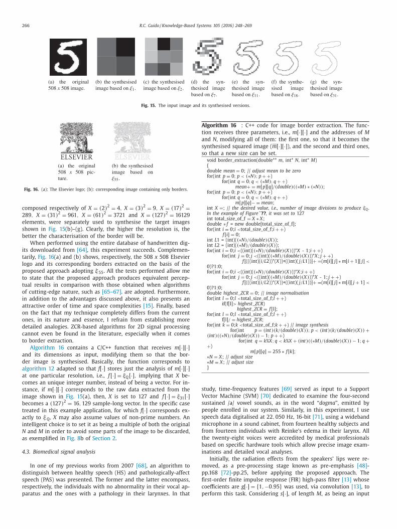
266 R.C. Guido / Knowledge-Based Systems 105 (2016) 248–269
Fig. 15. The input image and its synthesised versions.
Fig. 16. (a): The Elsevier logo; (b): corresponding image containing only borders.
Algorithm 16 : C++ code for image border extraction. The func-
tion receives three parameters, i.e., m [ ·][ ·] and the addresses of M
and N , modifying all of them: the first one, so that it becomes the
synthesised squared image ( m [ ·][ ·] ), and the second and third ones,
so that a new size can be set.
void border_extraction(double** m , int* N, int* M) { double mean = 0 ; // adjust mean to be zero for(int p = 0 ; p < (∗N) ; p + + )
for(int q = 0 ; q < (∗M) ; q + + ) mean + = m [ p][ q ] / (double )((∗M) ∗ (∗N)) ;
for(int p = 0 ; p < (∗N) ; p + + ) for(int q = 0 ; q < (∗M) ; q + + )
m [ p][ q ] − = mean ; int X = ; // the desired value, i.e., number of image divisions to produce ξQ . In the example of Figure˜ ?? , it was set to 127 int total_size_of_f = X ∗ X; double ∗ f = new double[total_size_of_f]; for(int i = 0 ; i < total_size_of_f; i + + )
f [ i ] = 0 ; int L 1 = (int)( (∗N) / (double )(X ) ); int L 2 = (int)( (∗M) / (double )(X ) ); for(int i = 0 ; i < ((int)( (∗N) / (double )(X ) ))* X - 1; i + + )
for(int j = 0 ; j < ((int)( (∗M) / (double )(X ) ))* X ; j + + ) f [(((int)( i/L 2 ))*( X))+((int)( j /L 1 ))] + = ( m [ i ][ j ] ∗ m [ i + 1][ j] <
0 )?1:0; for(int i = 0 ; i < ((int)( (∗N) / (double )(X ) ))* X ; i + + )
for(int j = 0 ; j < ((int)( (∗M) / (double )(X ) ))* X - 1; j + + ) f [(((int)( i/L 2 ))*( X))+((int)( j /L 1 ))] + = ( m [ i ][ j ] ∗ m [ i ][ j + 1] <
0 )?1:0; double highest _ ZCR = 0 ; // image normalisation for(int l = 0 ; l < total_size_of_f; l + + )
if(f[l] > highest _ ZCR ) highest _ ZCR = f [l];
for(int l = 0 ; l < total_size_of_f; l + + ) f[l] / = highest _ ZCR ;
for(int k = 0 ; k < total_size_of_f; k + + ) // image synthesis for(int p = (int)(k/ (double )(X )) ; p < (int)(k/ (double )(X )) +
(int)((∗N) / (double )(X )) − 1 ; p + + ) for(int q = k % X; q < k % X + (int)((∗M) / (double )(X )) − 1 ; q +
+ ) m [ p][ q ] = 255 ∗ f [ k ] ;
∗N = X; // adjust size ∗M = X; // adjust size }
s
V
s
p
s
m
f
t
b
i
m
p
fi
c
p
composed respectively of X = (2) 2 = 4 , X = (3) 2 = 9 , X = (17) 2 =289 , X = (31) 2 = 961 , X = (61) 2 = 3721 and X = (127) 2 = 16129
elements, were separately used to synthesise the target images
shown in Fig. 15 (b)–(g). Clearly, the higher the resolution is, the
better the characterisation of the border will be.
When performed using the entire database of handwritten dig-
its downloaded from [64] , this experiment succeeds. Complemen-
tarily, Fig. 16 (a) and (b) shows, respectively, the 508 x 508 Elsevier
logo and its corresponding borders extracted on the basis of the
proposed approach adopting ξ 55 . All the tests performed allow me
to state that the proposed approach produces equivalent percep-
tual results in comparison with those obtained when algorithms
of cutting-edge nature, such as [65–67] . are adopted. Furthermore,
in addition to the advantages discussed above, it also presents an
attractive order of time and space complexities [15] . Finally, based
on the fact that my technique completely differs from the current
ones, in its nature and essence, I refrain from establishing more
detailed analogies. ZCR-based algorithms for 2D signal processing
cannot even be found in the literature, especially when it comes
to border extraction.
Algorithm 16 contains a C/C++ function that receives m [ ·][ ·]and its dimensions as input, modifying them so that the bor-
der image is synthesised. Basically, the function corresponds to
algorithm 12 adapted so that f [ ·] stores just the analysis of m [ ·][ ·]at one particular resolution, i.e., f [ ·] = ξQ [ ·] , implying that X be-
comes an unique integer number, instead of being a vector. For in-
stance, if m [ ·][ ·] corresponds to the raw data extracted from the
image shown in Fig. 15 (a), then, X is set to 127 and f [ ·] = ξ31 [ ·]becomes a (127) 2 = 16 , 129 sample-long vector. In the specific case
treated in this example application, for which f [ ·] corresponds ex-
actly to ξQ , X may also assume values of non-prime numbers. An
intelligent choice is to set it as being a multiple of both the original
N and M in order to avoid some parts of the image to be discarded,
as exemplified in Fig. 8 b of Section 2 .
4.3. Biomedical signal analysis
In one of my previous works from 2007 [68] , an algorithm to
distinguish between healthy speech (HS) and pathologically-affect
speech (PAS) was presented. The former and the latter encompass,
respectively, the individuals with no abnormality in their vocal ap-
paratus and the ones with a pathology in their larynxes. In that
tudy, time-frequency features [69] served as input to a Support
ector Machine (SVM) [70] dedicated to examine the four-second
ustained /a/ vowel sounds, as in the word “dogma ”, emitted by
eople enrolled in our system. Similarly, in this experiment, I use
peech data digitalised at 22 , 050 Hz, 16-bit [71] , using a wideband
icrophone in a sound cabinet, from fourteen healthy subjects and
rom fourteen individuals with Reinke’s edema in their larynx. All
he twenty-eight voices were accredited by medical professionals
ased on specific hardware tools which allow precise image exam-
nations and detailed vocal analyses.
Initially, the radiation effects from the speakers’ lips were re-
oved, as a pre-processing stage known as pre-emphasis [48] -
p.168 [72] -pp.25, before applying the proposed approach. The
rst-order finite impulse response (FIR) high-pass filter [13] whose
oefficients are g[ ·] = { 1 , −0 . 95 } was used, via convolution [13] , to
erform this task. Considering s [ ·], of length M , as being an input

R.C. Guido / Knowledge-Based Systems 105 (2016) 248–269 267
Table 1
Results obtained from the experiment on biomedical signal analysis.
Value chosen for
C 19 .9% 24 .9% 33 .3%
Corresponding
value of T
� 100 C
� = � 100 19 . 9
� = 5 � 100 C
� = � 100 24 . 9
� = 4 � 100 C
� = � 100 33 . 3
� = 3
Corresponding
confusion matrix
PAS HS
PAS
HS
[7 0
0 7
] PAS HS
PAS
HS
[7 0
2 5
] PAS HS
PAS
HS
[6 1
1 6
]Resulting matrix
sensibility (% of
accuracy)
7+7 14
= 100% 7+5 14
= 85 . 71% 6+6 14
= 85 . 71%
s
s
L
o
t
s
m
a
l
i
t
s
f
p
i
t
n
o
r
e
b
t
m
t
r
g
f
v
1
e
e
P
C
b
p
a
t
a
I
t
a
d
i
F
c
i
c
l
5
c
Z
t
d
f
I
t
w
i
t
i
t
t
t
t
d
t
i
o
T
B
e
[
w
l
r
v
S
s
t
b
p
p
i
8
o
B
o
T
o
e
f
t
t
D
t
f
d
s
e
a
w
a
t
Z
3 Please, send requests to [email protected]
peech signal, the procedure is:
k ← s k − (0 . 95 · s k −1 ) , (1 � k < M) .
ikewise any usual classification scheme, this approach intends to
ffer the classifier a set of fixed-length feature vectors, implying
hat B 1 is useless. On the other hand, both B 2 and B 3 output a
et of T elements regardless of M , being the latter a preferable
ethod because it allows the regularity of ZCRs to be analysed
long a period. From Section 1.2 we have learnt that ZCRs are more
ikely to capture the fundamental frequencies of the speech signals,
.e., their pitch [12] ( F 0 ), disregarding the resonances of the vocal
ract, also known as being the formants ( F 1 , F 2 , ...), which corre-
pond to their higher frequencies. Complementarily, based on the
act that B 3 intrinsically normalises the frequencies it captures, the
roposed approach registers only the way pitches vary, disregard-
ng their values themselves. Thus, for any speaker, HS is expected
o keep an almost linear variation in response to the regular and
on-excessive effort performed by the vocal folds and associated
rgans during vibration. On the other hand, PAS usually shows ir-
egular variations due to an excessive, and sometimes irresponsive,
ffort perf ormed by the speakers’ vocal system.
Assuming that seven signals from each class were adopted as
eing their representative models and the other seven were used
o test the proposed approach, an ordinary absolute distance (AD)
easurement [73] was selected to serve as the classifier. The dis-
ances from each testing vector to all the template models are
egistered, then, the class for which the lowest one belongs to,
uides the assignment. Table 1 shows the best results obtained
or all the possible (
14 7
)2 = ( 14! 7!(14 −7)!
) 2 = (3432) 2 hold-out cross-
alidations procedures [74] , considering different options for C .
The respective accuracies suggest that a finer analysis, i.e., C =9 . 9% , is required to characterise important data. For C = 33 . 3% ,
xcessive information is grouped together in each of the T = 3 co-
fficients of the feature vectors, causing the misclassification of one
AS member that was labelled as being an HS one. Although for
= 24 . 9% , there are also incorrect assignments, HS members la-
elled as being PAS do not cause serious consequences, as in the
revious case in which the opposite occurs.
The above-mentioned characteristics of HS and PAS allow a rel-
tive generalisation of the results presented in Table 1 , despite
he modest size of the database, for which the lack of volunteers
nd the rigorous accreditations prevented further expansion. Thus,
consider a meaningful and relevant outcome was obtained. De-
ailed comparisons with similar state-of-the-art algorithms, such
s those documented in [68,75–79] , were avoided because their
atabases and pathologies differ, however, the proposed approach
s overall as accurate as, and much simpler than, those strategies.
urthermore, AD was purposely selected to play the role of the
lassifier just to emphasise the relevance of the ZCR-based features,
.e., due to the potential solution offered by the latter, the former,
onsisting of the simplest existing possibility, performs an effort-
ess job.
. Conclusions
This study, dedicated to our neurocomputing community, was
arefully written, polished and reviewed to serve as a tutorial on
CRs for both 1D and 2D DSP applications designed for PRKbS. All
he concepts I described correspond to the outcome of a wide and
etailed research work. The readers can observe that, despite the
act that ZCRs are well known in the literature, the different ways
show their applicability, majorly concerning the 2D cases, are to-
ally new.
Specifically, three methods for feature extraction based on ZCRs
ere presented just after the literature review section: B 1 , which
s the simplest one and is intended to produce variable-length fea-
ure vectors, is useful to search for a specific event or character-
stic in a digital signal, such as word segmentation or the distinc-
ion between voiced and unvoiced frames of a speech signal. B 2 , on
he other hand, for which an application on image border extrac-
ion based on analysis and re-synthesis was exhibited, is adopted
o inspect how ZCRs are distributed along the time, or space, in
ifferent levels of resolution. Finally, B 3 , exemplified for the dis-
inction of healthy and pathologically-affected biomedical signals,
s usefull in searching for the possible variabilities of ZCRs as time
r space advances. Three different types of normalisations, named
A, PA and EA, were also designed to work together with B 1 and
2 . Furthermore, sixteen algorithms, sixteen figures, six numerical
xamples and one table were included in the text.
The readers may have learnt from many references, such as
1] , that the ordinary PRKbS require a classifier to be associated
ith the features extracted from raw data. The more such features
inearly separate the mixed data from different classes in a cor-
ect manner, the less exquisite the classifier should be, and vice-
ersa. Particularly based on the example applications described in
ection 4 , I highlight one aspect of the proposed approaches: the
implest existing classifiers, i.e., HT and AD, were used, implying
hat the ZCR-based features brightly performed their work. Possi-
ly, this is due to the fact that ZCRs are, by themselves, neurocom-
uting agents, as shown in Section 2 . To treat much more com-
lex problems, the potential of ZCRs may be enlarged by associat-
ng them with different types of neural networks [80] , SVMs [ [81–
3] ], hidden markov models (HMMs) [84] , paraconsistent [85] , and
thers.
In relation to noisy inputs, B 3 is less influenced than B 1 and
2 when the noise, regardless of being white, pink, red, and so
n [7,13] , is uniformly distributed along the signal under analysis.
his is because that method describes the way ZCRs vary, instead
f counting them, implying that the artifacts introduced affect the
ntire signal more or less in the same manner, vanishing their ef-
ect over B 3 .
Concluding, the proposed approaches provide a valid contribu-
ion for both young researchers, who are expected to take advan-
age of the fundamental concepts and basic inputs drawn from
SP and PRKbS theory, and experienced professionals, for whom
his text may serve as an initial insight to the project of fruit-
ul and prominent algorithms. As mentioned in [1] , this study also
raws the DSP and PRKbS scientific communities’ attention to con-
ider the use of ZCRs, somewhen in conjunction with signal en-
rgy [1] or other features, to conform creativity, simplicity , and
ccuracy .
All the data used during the experiments, excluding TIMIT
hich is controlled by the Linguistic Data Consortium (LDC), are
vailable to the scientific community upon prior request 3 so that
he procedures could be reproduced. Further research related with
CRs focuses both on minor changes in the proposed approaches

268 R.C. Guido / Knowledge-Based Systems 105 (2016) 248–269
[
so that more specific issues are properly addressed. An intriguing
open question: are there humbler features than ZCRs which are ca-
pable of achieving similar or better results for basic spectral signal
description?
Acknowledgements
I am very grateful to CNPQ - “Conselho Nacional de Pesquisa e
Desenvolvimento”, in Brazil, for the grants provided, through the
process 306811/2014-6 , to support this research.
References
[1] R.C. Guido , A tutorial on signal energy and its applications, Neurocomputing
179 (2016) 264–282 . [2] J. Xu , A multi-label feature extraction algorithm via maximizing feature vari-
ance and feature-label dependence simultaneously, Knowl. Based Syst. 98
(2016) 172–184 . [3] Q. Zhou , H. Zhou , T. Li , Cost-sensitive feature selection using random forest: se-
lecting low-cost subsets of information features., Knowl. Based Syst. 95 (2016)1–11 .
[4] L. Yijing , Adapted ensemble classification algorithm based on multiple classi-fication systems and feature selection for classifying multi-class unbalanced
data., Knowl. Based Syst. 94 (2016) 88–104 .
[5] S. Garcia , J. Luengo , F. Herrera , Tutorial on practical tips of the most influentialdata preprocessing algorithm in data mining., Knowl. Based Syst. 98 (2016)
1–29 . [6] Y. Meng , J. Liang , Y. Qian , Comparison study of orthonormal representations of
functional data in classification., Knowl. Based Syst. 97 (2016) 224–236 . [7] S.M. Alessio , Digital Signal Processing and Spectral Analysis for Scientists: Con-
cepts and Applications, 1, Springer, 2016 . [8] B. Stroustrup , The C++ Programming Language, 4, Addison-Wesley Professional,
2013 .
[9] M. Steenbeck , A contribution to the behavior of short AC arcs during the cur-rent zero crossing., Z. Phys. 65 (1-2) (1930) 88–91 .
[10] F.M. Young , J.C. Grace , Zero crossing intervals of a sine wav in noise., J. Acoust.Soc. Am. 25 (4) (1953) 832 .
[11] J.P. Ertl , Detection of evoked potentials by zero crossing analysis., Electroen-cephalogr. Clin. Neurophysiol. 18 (6) (1965) 630–631 .
[12] L. Deng , D. O’Shaughnessy , Speech Processing: A Dynamic and Optimiza-
tion-oriented Approach, CRC Press, 2003 . [13] A.V. Oppenheim , R.W. Schafer , Discrete-time Signal Processing, 3, Prentice-Hall,
2009 . [14] S. Haykin , B.V. Veen , Signals and Systems, 2, Wiley, 2002 .
[15] S. Arora , Computational Complexity: a modern approach, Cambridge UniversityPress, 2009 .
[16] S. Goswami , P. Deka , B. Bardoloi , D. Dutta , D. Sarma , A novel approach for
design of a speech enhancement system using NLMS adaptive filter and ZCRbased pattern identification., in: Proceedings of the 2013 1st International Con-
ference on Emerging Trends and Applications in Computer Science (ICETACS),2013, pp. 125–129 . 13-14.
[17] H.-.M. Park , R.M. Stern , Spatial separation of speech signals using amplitudeestimation based on interaural comparisons of zero-crossings., Speech Com-
mun. 51 (1) (2009) 15–25 .
[18] A. Ghosal , R. Chakraborty , R. Chakraborty , S. Haty , B.C. Dhara , S.K. Saha ,Speech/music classification using occurrence pattern of ZCR and STE., in: Pro-
ceedings of the Third International Symposium on Intelligent InformationTechnology Application (IITA), 3, 2009, pp. 435–438 .
[19] R.R. Shenoy , C.S. Seelamantula , A zero-crossing rate property of power comple-mentary analysis filterbank outputs., IEEE Signal Process. Lett. 22 (12) (2015)
2354–2358 .
[20] A.V. Levenets , C.E. Un , Method for evaluating periodic trends in measuredsignals based on the number of zero crossings., Meas. Tech. 58 (4) (2015)
381–384 . [21] R.R. Shenoy , C.S. Seelamantula , Spectral zero-crossings: localization properties
and application to epoch extraction in speech signals., in: Proceedings of theInternational Conference on Signal Processing and Communications (SPCOM),
2012, pp. 1–5 .
[22] M. Jalil , F.A. Butt , A. Malik , Short-time energy, magnitude, zero crossing rateand autocorrelation measurement for discriminating voiced and unvoiced seg-
ments of speech signals., in: Proceedings of the International Conference onTechnological Advances in Electrical, Electronics and Computer Engineering
(TAEECE), 2013, pp. 208–212 . [23] R.G. Bachu , S. Kopparthi , B. Adapa , B.D. Barkana , Voiced/unvoiced decision for
speech signals based on zero-crossing rate and energy., in: K. Elleithy (Ed.), Ad-vanced Techniques in Computing Sciences and Software Engineering, Springer,
2010, pp. 279–282 .
[24] Y.-. I. Kim , H.-. Y. Cho , S.-. H. Kim , Zero-crossing-based channel atten-tive weighting of cepstral features for robust speech recognition: the ETRI
2011 CHiME challenge system., in: Proceedings of the Interspeech, 2011,pp. 1649–1652 .
[25] S.J. An , R.M. Kil , Y.-. I. Kim , Zero-crossing-based speech segregation and recog-nition for humanoid robots., IEEE Trans. Consum. Electron. 55 (4) (2009)
2341–2348 . [26] A.S. Zandi , R. Tafreshi , M. Javidan , Predicting epileptic seizures in scalp EEG
based on a variational bayesian gaussian mixture model of zero-crossing in-tervals., IEEE Trans. Biom. Eng. 60 (5) (2013) 1401–1413 .
[27] M. Phothisonothai , M. Nakagawa , A complexity measure based on modifiedzero-crossing rate function for biomedical signal processing., in: Proceedings
of the 13th International Conference on Biomedical Engineering (ICBME), 23,
2009, pp. 240–244 . [28] M.I. Khan , M.B. Hossain , A.F.M.N. Uddin , Performance analysis of modified zero
crossing counts method for heart arrhythmias detection and implementationin HDL., in: Proceedings of the International Conference on Informatics, Elec-
tronics and Vision (ICIEV), 2013, pp. 1–6 . [29] C.-. H. Wu , H.-. C. Chang , P.-. L. Lee , Frequency recognition in an SSVEP-based
brain computer interface using empirical mode decomposition and refined
generalized zero-crossing., J. Neurosci. Methods 196 (1) (2011) 170–181 . [30] D. Guyomar , M. Lallart , K. Li , A self-synchronizing and low-cost structural
health monitoring scheme based on zero crossing detection., Smart Mater.Struct. 19 (4) (2010) . Article Number: 045017, 2010.
[31] L. Florea , C. Florea , R. Vranceanu , C. Vertan , Zero-crossing based image pro-jections encoding for eye localization., in: Proceedings of the 20th European
Signal Processing Conference (EUSIPCO), 2012, pp. 150–154 .
[32] S. Watanube , T. Kotnatsu , T. Saito , A stabilized zero-crossing representation inthe wavelet transform domain and its extension to image representation for
early vision., in: IEEE TENCON - Digital Signal Processing Applications, 1996,pp. 496–501 .
[33] J.G. Daugman , Pattern and motion vision without laplacian zero crossings., J.Opt. Soc. Am. A-5 (7) (1988) 1142–1148 .
[34] K.-. L. Du , M.N.S. Swamy , Neural Networks and Statistical Learning, Springer,
2014 . [35] N. Nedjaha , F.M.G. Fran A§ a , M.D. Gregorio , L.M. Mourelle , Weightless neural
systems., Neurocomputing 183 (2016) 1–2 . [36] H.C.C. Carneiro , F.M.G. Franca , P.M.V. Lima , Multilingual part-of-speech tagging
with weightless neural networks., Neural Netw. 66 (2015) 11–21 . [37] G.G. Lockwood , I. Aleksander , Predicting the behaviour of g-RAM networks.,
Neural Netw. 16 (1) (20 03) 91–10 0 .
[38] T.F. Quatieri , Discrete-time Speech Signal Processing: Principles and Practice,Upper Saddle River, NJ: Prentice Hall, 2001 .
[39] W. Chou , B.H. Juang , Pattern Recognition in Speech and Language Processing,Boca Raton: CRC Press, 2003 .
[40] H. Beigi , Fundamentals of Speaker Recognition, New York: Springer, 2011 . [41] R.C. Guido , L.S. Vieira , S. Barbon Jr. , A neural-wavelet architecture for voice
conversion., Neurocomputing 71 (1-3) (2007) 174–180 .
[42] T. Ogunfunmi , M. Narasimha , Principles of Speech Coding, CRC Press, 2010 . [43] K. Skoruppa , et al. , The role of vowel phonotactics in native speech segmenta-
tion., J. Phonet. 49 (2015) 67–76 . 44] TIMIT speech corpus. linguistic data consortium (LDC), https://catalog.ldc.
upenn.edu/LDC93S1 . [45] C. Kim , K.-. d. Seo , Robust DTW-based recognition algorithm for hand-held
consumer devices., IEEE Trans. Consum. Electron. 51 (2) (2005) 699–709 . [46] X. He , L. Deng , Discriminative Learning for Speech Recognition, Morgan and
Claypool Publishers, 2008 .
[47] B. Atal , L. Rabiner , A pattern recognition approach to voiced-unvoiced-si-lence classification with applications to speech recognition., IEEE Trans. Audio,
Speech, Lang. Process. 1 (24) (1976) 201–212 . [48] J. Harrington , S. Cassidy , Techniques in Speech Acoustics, The Netherlands:
Kluwer Academic Publishers, 1999 . [49] O.J. Rosanen , U.K. Laine , T. Altosaar , An improved speech segmentation quality
measure: the r-value, in: Proceedings of the Interspeech, 2009, pp. 1851–1854 .
[50] S. Brognaux , T. Drugman , HMM-based speech segmentation: improvements offully automatic approaches., IEEE-ACM Trans. Audio, Speech, Lang. Process. 24
(1) (2016) 5–15 . [51] A. Stan , et al. , ALISA: an automatic lightly supervised speech segmentation and
alignment tool., Comput., Speech Lang. 35 (2016) 116–133 . [52] R.H. Baayen , C. Shaoul , J. Willits , M. Ramscar , Comprehension without segmen-
tation: a proof of concept with naive discriminative learning., Lang., Cognit.,
Neurosci. 31 (1) (2016) 106–128 . [53] F. Stahlberg , T. Schlippe , S. Vogel , T. Schultz , Word segmentation and pronun-
ciation extraction from phoneme sequences through cross-lingual word-to–phoneme alignment., Comput., Speech, Lang. 35 (2016) 234–261 .
[54] K.G. Estes , C. Lew-Williams , Listening through voices: infant statistical wordsegmentation and meaning acquisition through cross-situational learning., Dev.
Psychol. 51 (11) (2015) 1517–1528 .
[55] Ok. Rasanen , H. Rasilo , A joint model for word segmentation and meaningacquisition through cross-situational learning., Psychol. Rev. 122 (4) (2015)
792–829 . [56] L. White , S.L. Mattys , L. Stefansdottir , Beating the bounds: localised timing cues
for word segmentation., J. Acoust. Soc. Am. 138 (2) (2015) 1214–1220 . [57] F. Nery , J.S. Silva , N.C. Ferreira , F. Caramelo , R. Faustino , An algorithm for the
pulmonary border extraction in PET images, Proc. Technol. 5 (2012) 876–884 .
[58] L.H. Son , T.M. Tuan , A cooperative semi-supervised fuzzy clustering frameworkfor dental x-ray image segmentation, Expert Syst. Appl. 46 (2016) 380–393 .
[59] X.-. Y. Wang , Pixel classification based color image segmentation using quater-nion exponent moments., Neural Netw. 74 (2016) 1–13 .

R.C. Guido / Knowledge-Based Systems 105 (2016) 248–269 269
[
[
[
[
[
[
[
[
[
[
[
[[
[
[
[
[
60] M. Nixon , Feature Extraction & Image Processing for Computer Vision, 3, Aca-demic Press, 2012 .
[61] P. Zhang, T.D. Bui, C.Y. Suen, Wavelet feature extraction for the recognitionand verification of handwritten numerals., Keynote Address at 6th Interna-
tional Program on Wavelet Analysis and Active Media Technology. Availableat http://users.encs.concordia.ca/ ∼bui/pdf/Keynote.pdf .
62] S.E.N. Correia , J.M. Carvalho , R. Sabourin , On the performance of wavelets forhandwritten numerals recognition., in: Proceedings of the 16th International
Conference on Pattern Recognition, 2002, 3, 2002, pp. 127–130 .
63] X. You , L. Du , Y. Cheung , Q. Chen , A blind watermarking scheme using newnontensor product wavelet filter banks., IEEE Trans. Image Process. 19 (12)
(2010) 3271–3284 . 64] The MNIST database of handwritten digits, Available at http://yann.lecun.com/
exdb/mnist/ . 65] A. Pratondo , C.-. K. Chui , S.-.H. Ong , Robust edge-stop functions for edge-based
active contour models in medical image segmentation., IEEE Signal Process.
Lett. 23 (2) (2016) 222–226 . 66] Z.M. Hadrich A , A. Masmoudi , Bayesian expectation maximization algorithm by
using b-splines functions: application in image segmentation., Math. Comput.Simulat. 120 (2016) 50–63 .
[67] M. Liao , Automatic segmentation for cell images based on bottleneck detectionand ellipse fitting., Neurocomputing 173 (2016) 615–622 .
68] E. Fonseca , R.C. Guido , P.R. Scalassara , C.D. Maciel , J.C. Pereira , Wavelet
time-frequency analysis and least-squares support vector machine for theidentification of voice disorders., Comput. Biol. Med. 37 (4) (2007) 571–578 .
69] P. Addison , J. Walker , R.C. Guido , Time-frequency analysis of biosignals., IEEEEng. Biol. Med. Mag. 28 (5) (2009) 14–29 .
[70] R.O. Duda , P.E. Hart , D.G. Stork , Pattern Classification, 2, Wiley-Interscience,20 0 0 .
[71] M. Bossi , E. Goldberg , Introduction to Digital Audio Coding and Standards,
Kluwer, 2003 . [72] F. Muller , Invariant Features and Enhanced Speaker Normalization for Auto-
matic Speech Recognition, Logos Verlag, 2013 .
[73] V. Serdarushich , Analytic Geometry, CreateSpace Independent Publishing Plat-form, 2015 .
[74] J.H. Kim , Estimating classification error rate: repeated cross-validation, re-peated hold-out and bootstrap., Comput. Stat. Data Anal. 53 (11) (2009)
3735–3745 . 75] Z. Ali , I. Elamvazuthi , M. Alsulaiman , G. Muhammad , Detection of voice pathol-
ogy using fractal dimension in a multiresolution analysis of normal and disor-dered speech signals., J. Med. Syst. 40 (1) (2016) 1–10 .
[76] D. Panek , A. Skalski , J. Gajda , R. Tadeusiewicz , Acoustic analysis assessment
in speech pathology detection., Int. J. Appl. Math. Comput. Sci. 25 (3) (2015)631–643 .
[77] M. Alsulaiman , Voice pathology assessment systems for dysphonic patients:detection, classification, and speech recognition., IETE J. Res. 60 (2) (2014)
156–167 . 78] M.J. Pulga , A.C. Spinardi-Panes , S.A. Lopes-Herrera , L.P. Maximino , Evaluat-
ing a speech-language pathology technology., Telemed. e-health 20 (3) (2014)
269–271 . 79] T.L. Whitehill , S. Bridges , K. Chan , Problem-based learning (PBL) and
speech-language pathology: a tutorial., Clin. Linguist. Phonet. 28 (1-2) (2014)5–23 .
80] S. Haykin , Neural Networks and Learning Machines, 3, Prentice Hall, 2008 . 81] M. Jandel , Biologically relevant neural network architectures for support vector
machines., Neural Netw. 49 (2014) 39–50 .
82] Y. Leng , Employing unlabeled data to improve the classification performanceof SVM and its applications in audio event classification., Knowl. based Syst.
98 (2016) 117–129 . 83] L. Shen , Evolving support vector machines using fruit fly optimization for med-
ical data classification., Knowl. Based Syst. 96 (2016) 61–75 . 84] A.M. Fraser , Hidden Markov Models and Dynamical Systems, Society for Indus-
trial and Applied Mathematics, 2009 .
85] R.C. Guido , S. Barbon Jr. , R.D. Solgon , K.C.S. Paulo , L.C. Rodrigues , I.N. Silva ,J.P.L. Escola , Introducing the discriminative paraconsistent machine (DPM)., Inf.
Sci. 221 (2013) 389–402 .