ξy

ξz

η

ϕϕ '

x

ξ 'y

ξ 'z

z

zϕy

A BEAM FINITE ELEMENT MODEL INCLUDING WARPING

Application to the dynamic and static analysis of bridge decks

Diego Lisi

Dissertação para obtenção do Grau de Mestre em

Engenharia Civil

Júri

Presidente: Doutor José Manuel Matos Noronha da Câmara

Orientador: Doutor Francisco Baptista Esteves Virtuoso

Co-orientador: Doutor Ricardo José de Figueiredo Mendes Vieira

Vogal: Doutor Luís Manuel Coelho Guerreiro

Outubro de 2011

iii

RESUMO

Esta dissertação tem como objectivo o estudo dos efeitos dinâmicos e estáticos em vigas contínuas com

secçôes de parede fina através do desenvolvimento de um modelo de elementos finitos.

Quando uma secção de parede fina é aberta a sua deformabilidade é consideravelmente maior do que a da

secção compacta, devido à deformação da secção de parede fina no seu próprio plano quando sujeita à torção,

sendo este efeito devido ao empenamento da secção.

A análise exacta de vigas com parede fina considerando o fenómeno do empenamento é complexa na sua

implementação numérica, geralmente por causa das soluções matemáticas serem muito exigentes em termos

computacionais.

As teorías clássicas de vigas são analizadas inicialmente por forma a obter a formulação das equacções

governativas dos deslocamentos. Os princípios variacionais são utilizados para a determinação de um modelo

aproximado e na caracterização de um elemento finito de viga para a análise das secções de parede fina.

No ambito da estática, vigas contínuas com eixo rectilíneo são analisadas; em dinâmica, a vibração lateral e

torsional destes elementos é investigada quer em regime livre quer quando o sistema estrutural é sujeito à

aplicação de uma carga móvel. Os resultados destas análises são comparados com as equaçoes teóricas de vigas.

O objectivo deste trabalho é o de propôr um modelo de viga generalizado para secções de parede fina para a

análise e o projecto de pontes ferroviárias de alta velocidade. Um caso de estudo de ponte com vários tramos é

ilustrado para avaliar o desempenho dinâmico de diferentes secções.

PALAVRAS CHAVE: secções de parede fina, tabuleiro de ponte, método dos elementos finitos,

empenamento, elemento de viga, análise dinâmica, cargas móveis.

v

ABSTRACT

The present dissertation deals with the study of the dynamic and static effects on continuous beams of thin-

walled cross-sections through the formulation a of a finite element.

When a thin-walled cross-section of a beam structure has open profile the deformability greatly exceeds that

of a compact section, because of to the out-of-plane deformations of this type of shapes when acted by torsion,

being this effect due to the warping of the cross-section.

The exact analysis of thin walled beams considering the warping phenomena is usually difficult in its

implementation by numerical codes for their mathematical solutions that are too complicated for routine

calculations.

The classic beam theories are analyzed to obtain the set of equations governing the problem. The variational

principles are used in order to obtain an approximation model and purpose a finite beam element for the

analysis of thin-walled beams.

In static, straight and generally supported structures are analyzed, while in dynamic the torsional and lateral

free-vibration and forced vibration is investigated. The results of the analysis and the compliance with the classic

beam theory are discussed.

The aim of the work is to propose a generalized thin-walled beam model for the railway high-velocity bridge

analysis and design. A simple numerical example of multi-span bridge is illustrated in order to evaluate the

performance of different types of cross-sections when dynamic effects are considered.

KEYWORDS: thin-walled beams, bridge deck, finite element method, warping, beam element, dynamic

analysis, moving load.

vii

ACKNOWLEDGEMENTS

I would like to express my gratitude for all who contributed in a way or another in the accomplishment of

this work.

Most importantly, I would like to thank my supervisors Pr. Francisco Virtuoso and Pr. Ricardo Vieira. Their

helpful comments, advices, suggestions and contributions regarding all the critical aspects of my thesis have

been very profitable over the last year.

I would thank all the colleagues of the Civil Engineering (DECivil) department for being extremely helpful

and for creating a comfortable working environment. Their friendship has provided a real support.

Many thanks for my family: they made it possible for me to come to Lisbon.

ix

INDEX

RESUMO ........................................................................................................................................................................................................... iii

ABSTRACT ......................................................................................................................................................................................................... v

ACKNOWLEDGEMENTS ........................................................................................................................................................................... vii

1. INTRODUCTION .............................................................................................................................................................................. 17

1.1. General introduction ................................................................................................................................................................... 17

1.2. Objectives of the work ................................................................................................................................................................ 17

1.3. Layout of the work ........................................................................................................................................................................ 18

1.4. Original contributions of the present work ....................................................................................................................... 18

2. LITERATURE REVIEW AND BACKGROUND INFORMATION ...................................................................................... 21

2.1. Historical evolution of thin walled beam theories ......................................................................................................... 21

2.2. Methods of analysis for thin walled beam structures ................................................................................................... 22

2.3. Lateral-torsional forced vibrations of thin walled beam structures ...................................................................... 23

3. THIN-WALLED BEAMS EQUATIONS ..................................................................................................................................... 25

3.1. Cross-section analysis ................................................................................................................................................................. 25

3.1.1. Kinematics and strains ...................................................................................................................................................... 25

3.1.2. Potential energy formulation ......................................................................................................................................... 31

3.1.3. Elastic center and shear center ..................................................................................................................................... 35

3.1.4. Kinetic energy formulation ............................................................................................................................................. 36

3.2. Static analysis ................................................................................................................................................................................. 38

3.2.1. Equilibrium and stresses .................................................................................................................................................. 38

3.2.3. Basic load cases .................................................................................................................................................................... 43

3.3. Dynamic analysis ........................................................................................................................................................................... 53

3.3.1. Equations of motion ........................................................................................................................................................... 53

3.3.2. Analysis of torsional free vibrations on thin-walled beams ............................................................................. 57

4. FINITE ELEMENT APROXIMATION ....................................................................................................................................... 61

4.1. Beam displacements discretization ...................................................................................................................................... 61

4.1.1. Continuity ................................................................................................................................................................................ 62

4.1.2. Approximation functions.................................................................................................................................................. 62

4.2. The static formulation of the finite element...................................................................................................................... 64

4.2.1. The formulation of a weak form for uncoupled torsion ..................................................................................... 65

4.2.2. The thin-walled beam element considering an additional DOF of warping .............................................. 68

4.2.3. Selected load cases .............................................................................................................................................................. 76

x

4.3. The dynamic formulation of the finite element ............................................................................................................... 92

4.3.1. The formulation of a weak form for the uncoupled torsion ............................................................................. 93

4.3.2. The element mass matrix considering an additional DOF of warping ......................................................... 94

4.3.3. The undamped Free vibration .................................................................................................................................... 101

4.3.4. Examples ............................................................................................................................................................................... 103

5. ANALYSIS OF DYNAMIC RESPONSE TO MOVING LOADS ......................................................................................... 113

5.1. The procedure of mode superposition ............................................................................................................................. 113

5.1.1. Uncoupled equations of motion with damping ................................................................................................... 114

5.1.2. Modal response to loading ............................................................................................................................................ 115

5.2.Numerical modeling of dynamical response ................................................................................................................... 116

5.2.1.Element property matrices............................................................................................................................................ 116

5.2.2.Time-stepping Newmark’s method ........................................................................................................................... 118

5.3. Numerical example .................................................................................................................................................................... 119

5.3.1.Actions on the bridge and structural properties ................................................................................................. 119

5.3.2.Undamped free-vibration analysis ............................................................................................................................. 121

5.3.3.Forced-vibrations analysis and mode-superposition procedure ................................................................. 123

6. CONCLUSIONS AND FINITE DEVELOPMENTS ............................................................................................................... 137

6.1. General remarks ......................................................................................................................................................................... 137

6.1. Conclusions ................................................................................................................................................................................... 137

6.2. Future developments ............................................................................................................................................................... 138

7. References ...................................................................................................................................................................................... 141

ANNEX 1 ....................................................................................................................................................................................................... 143

xi

INDEX OF FIGURES Figure 3.1 - Principal displacements and system coordinates of the beam. ..................................................................... 26

Figure 3.2 - Rotation of a I-Section around a general point P. ................................................................................................ 26

Figure 3.3- Axial displacements of an I-Beam due to axial effect and bending for planes (x,y) and (x,z). .......... 27

Figure 3.4 - Vanishing of the shear strain of mid-surface (left) and distribution along the wall thickness for

open cross-sections (right). ............................................................................................................................................................................ 27

Figure 3.5 - Rotation of open cross-section. .................................................................................................................................... 28

Figure 3.6 – Geometric interpretation of the sectorial coordinate. ...................................................................................... 29

Figure 3.7 – Geometric interpretation of h(s) and hs(s). ........................................................................................................... 31

Figure 3.8 – Generalized displacements of a C cross-section beam. .................................................................................... 43

Figure 3.9 – Forces in a C cross-section beam. ............................................................................................................................... 43

Figure 3.10 – S-S beam (L=2m) acted upon uniform torque. .................................................................................................. 46

Figure 3.11 - � value of a S-S beam acted by uniform torque (analytical solution). ..................................................... 47

Figure 3.12 – �′ value of a S-S beam acted by uniform torque (analytical solution). ................................................... 47

Figure 3.13 - �� of a S-S beam acted by uniform torque (analytical solution). ............................................................. 47

Figure 3.14 – Distribution of the torsion �� and � of a S-S beam acted by uniform torque (analytical

solution). .................................................................................................................................................................................................................. 48

Figure 3.15 – S-S beam (L=2m) acted upon concentrated torque at midspan. ............................................................... 48

Figure 3.16 – � value of a S-S beam acted by concentrated torque (analytical solution). ......................................... 49

Figure 3.17 – �′ value of a S-S beam acted by concentrated torque (analytical solution). ........................................ 49

Figure 3.18 – �� of a S-S beam acted by concentrated torque (analytical solution). ................................................. 49

Figure 3.19 - Distribution of the torsion �� and � of a S-S beam acted by concentrated torque (anal. solution).

...................................................................................................................................................................................................................................... 50

Figure 3.20 – Three continuous span beam acted by uniform torque at midspan. ....................................................... 50

Figure 3.21 – � value of a continuous three spans beam acted by uniform torque (analytical solution). .......... 51

Figure 3.22 – �′ value of a continuous three spans beam acted by uniform torque (analytical solution). ........ 51

Figure 3.23– ��of a continuous three spans beam acted by uniform torque (analytical solution). .................... 52

Figure 3.24 - Distribution of the torsion �� and � of a continuous three spans beam acted by uniform torque

(analytical solution). ........................................................................................................................................................................................... 52

Figure 3.25 – Distribution of the torsion �� and � of a continuous three spans beam acted by uniform

torque (analytical solution). ........................................................................................................................................................................... 52

Figure 3.26 – Coupling between torsion and bending displacements for a C-beam. .................................................... 57

Figure 3.27 – Simply supported beam analyzed by (Gere, 1954). ........................................................................................ 58

Figure 3.28 – Values of the ratio r for the first 8 torsional vibration modes. ................................................................... 59

Figure 4.1 – Degrees of freedom and shape functions of the two node elements. ......................................................... 63

Figure 4.2 - Two-node Euler-Bernoulli element. ...................................................................................................................... 64

Figure 4.3 –Thin walled beam element subject to uncoupled torsion. ............................................................................... 68

Figure 4.4 – Effects of the application of a general axial force on a thin walled beam (Cedolin, 1996). .............. 70

Figure 4.5 – Thin-walled C-beam element displacement referred to two axis. .............................................................. 74

Figure 4.6 –Thin-walled C-beam element displacements described by the elastic center axis. .............................. 76

xii

Figure 4.7 – Non-dimensional coordinate system. ....................................................................................................................... 77

Figure 4.8 – � value of a S-S beam acted by uniform torque (FEM solution). ................................................................. 77

Figure 4.9 – �′ value of a S-S beam acted by uniform torque (FEM solution). ................................................................ 78

Figure 4.10 - �� of a S-S beam acted by uniform torque (FEM solution). ....................................................................... 78

Figure 4.11 – Torsion � of a S-S beam acted by uniform torque (FEM solution). .......................................................... 78

Figure 4.12 – � value of a S-S beam acted by concentrated torque (FEM solution). .................................................... 79

Figure 4.13 – �′ value of a S-S beam acted by concentrated torque (FEM solution). ................................................... 79

Figure 4.14- �� of a S-S beam acted by concentrated torque (FEM solution). .............................................................. 79

Figure 4.15 - Torsion � of a S-S beam acted by concentrated torque (FEM solution). ................................................ 80

Figure 4.16 – Coordinate system of the three continuous spans beam. ............................................................................. 80

Figure 4.17 - � value of a T-C-S beam acted by uniform torque (FEM solution). ........................................................... 81

Figure 4.18 - �′ value of a T-C-S beam acted by uniform torque (FEM solution). ......................................................... 81

Figure 4.19 - �� of a T-C-S beam acted by uniform torque (FEM solution). ................................................................... 81

Figure 4.20 – Tosion � of a T-C-S beam acted by uniform torque (FEM solution). ....................................................... 82

Figure 4.21 – Convergence of the �� value as function of the mesh refinement. ........................................................ 83

Figure 4.22 – ABAQUS element B310S and integration points for I-beam section. ...................................................... 83

Figure 4.23 - Longitudinal model of a bridge numerical example. ....................................................................................... 85

Figure 4.24 – Box-section of the bridge deck. ................................................................................................................................ 85

Figure 4.25 – Double-T section of the bridge deck. ..................................................................................................................... 85

Figure 4.26 – Lane model for general types of vertical loads. ................................................................................................. 86

Figure 4.27 – Loading in the cross-section plane. ........................................................................................................................ 88

Figure 4.28 –Loading in the longitudinal direction. .................................................................................................................... 88

Figure 4.29 – Coupling effect between torsion and transversal displacement. .............................................................. 88

Figure 4.30 – Displacements and rotation of the bridge model with double-T section (FEM model). ................. 89

Figure 4.31 – Shear force � and bending moment � along the elastic center axis. ................................................. 90

Figure 4.32 – Torsion moment � and warping moment �� along the elastic center axis. .................................... 90

Figure 4.33 - Twist values along the beam axis for the double-T section and for the Box section. ........................ 91

Figure 4.34 – Saint Venant torsion contribution for the double-T section and for the Box section. ..................... 91

Figure 4.35 – Warping torsion influence in torsion response for different �-values (FEM solution)................... 92

Figure 4.36 –Thin-walled C-beam element and uncoupled kinematic field. .................................................................... 99

Figure 4.37 - Thin-walled C-beam element and coupled kinematic field. ...................................................................... 101

Figure 4.38 - Ratio r for 8 vibration modes in a S-S beam. Solution obtained by the presented model. .......... 105

Figure 4.39 - Ratio r for 8 vibration modes in a C-S beam. Solution obtained by the presented model. ......... 105

Figure 4.40 - Ratio r for 8 vibration modes in a C-C beam. Solution obtained by the presented model. ......... 106

Figure 4.41 - Influence of boundary conditions on the 1st mode frequency. ................................................................. 107

Figure 4.42 - Influence of boundary conditions on the 2nd mode frequency. .............................................................. 107

Figure 4.43- Influence of boundary conditions on the 3rd mode frequency................................................................. 107

Figure 4.44 - Influence of boundary conditions on the 4th mode frequency. ............................................................... 108

Figure 5.1 – Example of supported beam element acted by a constant and eccentric moving load. ................. 115

Figure 5.2 – Experimental values of the damping coefficient for different bridge spans. (Cunha, 2007). ....... 117

xiii

Figure 5.3 – Applied loads on a supported beam along �-direction. ................................................................................ 117

Figure 5.4 – Linear interpolation for the time intensity at time t....................................................................................... 118

Figure 5.5 – Bridge layout of the cross-section and sketch of the actions considered. ............................................ 120

Figure 5.6 – Damping coefficients variation for the double-T bridge section. ............................................................. 124

Figure 5.7 – Damping coefficients variation for the box girder bridge section. ........................................................... 124

Figure 5.8 – Layout of the simply supported beam and moving load............................................................................... 125

Figure 5.9 – Mid-span dimensionless displacement comparison ( = 0.5). .................................................................. 126

Figure 5.10 – Mid-span dimensionless displacement comparison ( = 1). ................................................................... 126

Figure 5.11 – Mid-span dimensionless displacement comparison ( = 2). ................................................................... 126

Figure 5.12 - Mid-span dimensionless displacement comparison ( = 0.5, � = 0.1). ............................................... 127

Figure 5.13 - Mid-span dimensionless displacement comparison ( = 1, � = 0.1). ................................................... 127

Figure 5.14 - Mid-span dimensionless displacement comparison ( = 2, � = 0.1). ................................................... 127

Figure 5.15 – Longitudinal beam-like model (a) and layout of the cross-section analyzed (b). .......................... 128

Figure 5.16 – Dynamic influence lines of the displacement uz at the section AA’ (double-T section). ............. 129

Figure 5.17 - Dynamic influence lines of the twist φ at the section AA’ (double-T section). ................................. 129

Figure 5.18 - Dynamic influence lines of the displacement uy at the section AA’ (double-T section). .............. 130

Figure 5.19 - Dynamic influence lines of the displacement uz at the section AA’(box girder section).. ............ 130

Figure 5.20 - Dynamic influence lines of the twist φ at the section AA’ (box girder section). .............................. 131

Figure 5.21 - Dynamic influence lines of the displacement uy at the section AA’ (box girder section). ........... 131

Figure 5.22 – Displacement � for the two bridge sections analyzed (load speed: 420 km/h). .......................... 131

Figure 5.23 – Horizontal displacements of the bridge cross-section(load speed: 420 km/h). ............................. 132

Figure 5.24 - Twist of the bridge sections (load speed: 420 km/h). ................................................................................. 132

Figure 5.25 – Maximum vertical deflection of the section AA’ for various speed values. ........................................ 133

Figure 5.26 – Maximum twist rotation of the section AA’ for various speed values. ................................................. 133

Figure 5.27 – Displacement of the point P of the double-T section. .................................................................................. 134

Figure 5.28 – Dynamic influence line of the displacement ��. ......................................................................................... 134

Figure A.0.1 – Cross-section layouts ................................................................................................................................................ 143

Figure A.0.2 – Sectorial coordinate for the open and closed cross-sections. ................................................................ 143

Figure A.0.3 – Cartesian coordinates referred to the elastic center. ................................................................................. 144

xv

INDEX OF TABLES

Table 2.1 – Analogy between the theories of Vlasov and Bernoulli. .................................................................................... 21

Table 3.1 - Cross-Section parameters. ............................................................................................................................................... 33

Table 3.2 – Beam loads per unit length. ............................................................................................................................................ 34

Table 3.3 – Equilibrium equations and boundary conditions. ................................................................................................ 42

Table 3.4 - Cross-section layouts and position of the elastic and shear center. .............................................................. 45

Table 3.5 – Boundary conditions for the three continuous spans beam. ........................................................................... 50

Table 3.6 – Dimensionless warping moment at supports. ........................................................................................................ 52

Table 3.7 – Characteristics of the beam element analyzed by (Gere, 1954). .................................................................... 58

Table 4.1 – Smoothness of functions (Fish & Belytschko, 2007). .......................................................................................... 62

Table 4.2 – Displacement field and approximation functions. ................................................................................................ 69

Table 4.3 – Beam element displacements and corresponding axis of reference ............................................................ 73

Table 4.4 – Cross-section layout characteristics. .......................................................................................................................... 77

Table 4.5 – Boundary conditions of the beam. ............................................................................................................................... 77

Table 4.6 – FEM discretization for the continuous three spans beam. ............................................................................... 80

Table 4.7 – Boundary conditions of the three continuous spans beam. ............................................................................. 80

Table 4.8 – Decrease of the relative error of ��/��2 for different finite element meshes. ................................... 82

Table 4.9 – Characteristics of the beam Elements loaded. ....................................................................................................... 84

Table 4.10 – Comparison of results between current model and ABAQUS element. ................................................... 84

Table 4.11 – Flexural characteristics of the bridge deck cross-sections. ........................................................................... 86

Table 4.12 – Section properties of the bridge cross-sections.................................................................................................. 87

Table 4.13 – Cross-section properties and torsion parameters. ............................................................................................ 87

Table 4.14 – Boundary displacement fixed at nodes. ................................................................................................................. 89

Table 4.15 – Boundary conditions of the bar (S-S,C-S,C-C). .................................................................................................. 104

Table 4.16 – Characteristics of the steel beam cross-section layout and bar length. ................................................ 109

Table 4.17 – Torsional vibration modes for a simply supported I-beam. ....................................................................... 109

Table 4.18 - Characteristics of the cross-section layout and span lengths. .................................................................... 110

Table 4.19 - Torsional vibration modes for a three continuous spans I-beam. ........................................................... 110

Table 4.20 – Characteristics of the cross-sections and structural systems compared. ............................................ 111

Table 4.21 – Mode vibration frequencies for the S-S beam and relative errors compared with ABAQUS. ...... 111

Table 4.22 – Mode vibration frequencies for the T-C-S beam and relative errors compared with ABABUS. . 111

Table 5.1 – General actions of the railway bridge. .................................................................................................................... 120

Table 5.2 – Undamped vibration modes and respective modal frequencies for the double-T bridge section.

................................................................................................................................................................................................................................... 121

Table 5.3 – Vibration modes for the double-T bridge section (frequencies in [Hz]). ................................................ 122

Table 5.4 – Undamped vibration modes and respective modal frequencies for the box bridge section. ......... 123

Table 5.5 – Rayleigh coefficients for the bridge cross-sections considered. ................................................................. 124

Table 5.6 – Properties of the simply supported beam-like bridge discretization. ...................................................... 125

Table 5.7 – Set of train velocities considered. ............................................................................................................................. 128

xvi

Table 5.8 – Parameters considered for the numerical simulation of the current analysis. .................................... 129

Table 5.9 – Maximum displacement values for some characteristic velocities. ........................................................... 133

Table 5.10 – Maximum twist values for some characteristic velocities. ......................................................................... 133

17

1. INTRODUCTION

1.1. General introduction

Throughout history, thin walled structures become common construction elements. The reason for their

extensive use is probably due to the trend of reducing the structural weight and to minimize building materials.

This very natural optimization strategy constituted an important design principle for the realization of any type

of structure.

For the large use of thin walled sections their behavior have been widely studied from many authors and the

simplest way to consider these elements, when involved in frame structures analysis, is the adoption of

longitudinal beam elements. This is possible whenever the response of slender elements is investigated, such as

the analysis of steel structures, buildings, bridges or other complex structures.

The thin walled cross-sections appear in different forms, from simple hot rolled steel beams to the complex

hull of a ship or the bridge deck shape. In all these cases the knowledge of flexural, axial and torsional response is

essential for the analysis of the internal forces and the stress field acting on the sections.

The present analysis considers railway bridges with a cross-section that can be considered thin-walled. For

these structures, the torsion has a very important role to investigate their structural response. It is well known

that the torsional response of a thin-walled open section is very different from that of a compact or closed shaft.

When the section of a bridge has an open profile the out-of-plane longitudinal deformations greatly exceed those

of a closed section, either in a multicellular or in a monocellular type. This happens because of the physical

behavior of this kind of shapes in their response to torsion solicitations: for this reason, in the field of bridges

and advanced constructions, torsion is an important aspect to be considered in the design and the warping of the

open sections cannot be neglected.

Warping introduces longitudinal strains as the section twists and significantly affects the torsional stiffness.

In the case of thin-walled beams with open cross-section, the constraint of the axial warping strains provides the

primary source of torsional stiffness.

1.2. Objectives of the work

The dynamic study of railway bridges has been greatly enhanced during the recent years: the means of

transport are faster and heavier, while the structure over which they move are more slender and generally

constituted by thin-walled cross sections.

This study presents a generalized beam model based on the FEM1 technology for the static and dynamic

analysis of thin-walled beams. According to the Euler-Bernoulli theory, six degrees of freedom for each end of the

finite element are considered. A 7th degree of freedom will be considered in the finite element developed in order

to describe the warping displacements.

1 Finite element method

18

The consideration of the cross section warping is based on the Vlasov beam theory for thin walled open

sections and extended to the closed thin-walled section by introducing a modified warping parameter according

to the Benscoter theory.

In statics, straight and generally supported structures are analyzed, while in dynamics the torsional and

lateral free and forced vibration analysis is presented. In the last part of the work an example of moving force

acting eccentrically is presented, in order to evaluate the performance of this type of elements in bridge design.

The focus of the work is the analysis of double-T bridge open sections and box girder sections. An uncoupled

flexural motion in the vertical plane and a coupled lateral-torsional vibration are studied showing the effect of

the sectional properties on the mode frequencies. When forced vibration are considered, this work obtains

dynamic influence lines for the twist rotation, the horizontal and vertical displacement of the midspan point for

different train velocities, load magnitudes and eccentricity. The purpose is the formulation of a simple tool that

enables the basic analysis of multi-span bridges through adequate beam models that consider the thin-walled

open or closed section effects.

1.3. Layout of the work

In chapter 1 a general introduction to the current work is presented. The motivations and developments

needed are illustrated considering the contribution of the thin walled beam elements to the civil engineering

applications.

The chapter 2 proposes a general review of the thin-walled beam theories with particular attention to the

torsion problem considering the different cross-section behaviors. A general survey summarizes also the

application in dynamic analysis of these studies and the results obtained with the theoretical approach.

The chapter 3 presents the theory of thin-walled beams in statics and dynamics. Starting from the

description of the beam element kinematics, the governing differential equations for thin-walled cross-sections

are deduced by using the energetic approach. Several load cases are presented in static analysis considering the

exact results, while in dynamics a torsional vibration analysis is presented.

The chapter 4 deals with the assembling of a finite beam element for the extensional, lateral and torsional

analysis. The element property matrices are formulated from the thin-walled beam governing equations. The

static analysis for some load cases are presented and the convergence of the element discretization is discussed.

In dynamic the free-torsional vibration modes are presented for practical problems.

In chapter 5 a practical load case is developed. The aim of the study is the analysis of the bridge deck

response to moving forces acting eccentrically along a multi-span longitudinal layout. The results obtained with

the approximated method are compared with those of the theoretical analysis.

1.4. Original contributions of the present work

Thin-walled structures have gained a growing importance due to their efficiency in strength and cost and for

this reason several applications in the high-speed railway bridges design have been recently developed. Many

19

studies of bridge dynamic behavior have been performed using a so-called macro-approach. In this technique,

the bridge system is discretized into a number of beam-column or grid elements and the focus is on forces rather

than on stresses. The elements can be straight or curved and an analysis example is given by (Okeil & S., 2004).

The method of analysis presented in this work is the space frame approach, which falls under the macromodel

category.

The aim of this work is to develop a model for the static and dynamic analysis of one-dimensional straight

beam structures with thin-walled cross-sections, extended for general conditions of supports and generalized

applied loads. This type of element is suitable for the computer simulation of the results by the classic principles

of the FEM technology.

The Vlasov’s beam theory is adopted for the formulation, through the variational principles of a finite beam

element with open cross-section. The polynomial Hermite’s interpolation is used to obtain approximated results

in static and dynamic analysis, using only one element type for open or closed cross-section. The only difference

is that for the closed sections a warping function according to Benscoter’s theory is considered.

In statics, examples of commonly loaded beams are studied and the exact solutions are approximated by

means of an h refinement type of the element mesh.

In dynamics, the problem of free vibration is approached by modal analysis criteria for generally supported

beams and a forced vibration numerical example is developed by using the mode superposition method (Clough

& Penzien, 1982). The equation of motion are then integrated by the Newmark’s step-by step method. The

maximum values of displacement and rotation are found for common bridge deck cross-sections as a function of

the train velocity and a series of dynamic influence lines are derived.

This kind of analysis, especially in dynamics, is useful for modeling straight beam structures and the

consideration of thin-walled beam elements theory for illustrating open-section’s response is a research field

still in development, where the civil engineering recent means of analysis, such as the computer simulation of

results, could develop a powerful contribution.

21

2. LITERATURE REVIEW AND BACKGROUND INFORMATION

The aim of this chapter is to synthesize and discuss the accredited knowledge established from the

literature, related to the main concepts of the present work. The theory of thin-walled beam elements is

presented in 2.1 with all the developments made. Then a survey of the FEM approximations studied for solving

the static and dynamic problem of beam structures is also presented in 2.2 and 2.3. The chapter concludes with

section 2.4 by highlighting the original contribution of this work to the overviewed research fields.

2.1. Historical evolution of thin walled beam theories

The behavior of thin-walled elements has been extensively studied by the theories of elastic beams. For

arbitrary profiles, loading cases and boundary conditions, an important non uniform torsional warping occurs,

hence the Saint Venant torsional theory, which is strictly restricted to uniform torsion with free warping of the

cross-section, is no longer sufficient. A thin walled member resists to non uniform warping by both normal and

shear stresses. If these stresses are important, an extended theory for non-homogeneous torsion is needed.

The general theory of thin-walled open cross-sections was developed in its final form by (Vlasov, 1961)

where the non-uniform warping deformation effect is considered through the definition of a sectorial coordinate,

while the transverse shear strain is neglected.

Thus, the sectorial coordinate is obtained by neglecting the transverse shear deformations through the wall

thickness. The exact stress distribution is found by using Saint-Venant theory, but the beam equilibrium is

ensured by introducing Vlasov bimoment. This is admissible for open cross-section but the theory becomes more

complex when closed thin-walled section are considered, because the shear stresses are statically indeterminate.

In table 2.1 is shown the analogy between Vlasov theory and Bernoulli beam theory.

Table 2.1 – Analogy between the theories of Vlasov and Bernoulli.

Vlasov theory of non-uniform torsion Correspondent of the Bernoulli beam theory

Warping moment Bending moment

Warping torsion Shear

Twist angle Transversal displacement in the flexural plan

Twist gradient along the beam axis Gradient of the transversal displacement

Warping function Displacement distribution over the cross-section area

(Benscoter, 1954) introduced a new sectorial coordinate, where the shear transverse strains are no longer

neglected and a fictitious shear deformation is introduced. Benscoter theory characterizes the warping degree of

freedom by an independent function which is different from the gradient of the torsional angle.

All the cases in which uniform and non-uniform torsion are present represent the so called “mixed torsion

problems”. Many other authors studied this kind of problem and with different approaches. When the hypothesis

of cross section non-deformability is relaxed, additional modes called distortional modes are added to the classic

ones describing the behavior of a thin-walled beams: tension/compression, bending and torsion. These

additional modes are related to the in-plane deformation of a thin-walled cross section.

22

Important progress has been recently made by using different numerical methods: beam elements are

defined using beam theory with a single warping function valid for arbitrary geometry of cross sections, without

any distinction between open or closed profiles and without using sectorial coordinates. The results obtained

have been compared for stability analysis of beams (Saadé, Espion, & Warzée, 2003).

2.2. Methods of analysis for thin walled beam structures

The analysis of thin-walled beam with arbitrary section are recently approached considering either the

principle of virtual displacements or using variational principles. These methods are suitable for automatic

computation of three-dimensional straight beam elements.

Different stiffness methods have been presented for closed cross-sections considering the Benscoter’s

assumption in the static (Prokić, 2002) and in dynamic (Prokić & Lukić, 2007) structural analysis. In this theory

the function that defines warping intensity represents a new unknown that may be derived as a function of the

angle of rotation of the profile. (Shakourzadeh, Guo, & Batoz, 1993) formulate a finite element for the static

analysis of open and closed thin-walled sections, using the same initial assumptions. An exact hybrid element is

formulated accounting the exact solution by non-polynomial interpolation functions.

In static analysis, the theories of bending and torsion are often compared in the literature by pointing out an

analogy between Bernoulli bending theory and Vlasov torsional theory for open cross sections. (Kollbrunner &

Basler, 1969) shows this analogy by analyzing commonly supported beams examples. All the internal forces in

terms of warping moments refers to different cross-section types and the results are illustrated for different load

cases, in order to establish a classification for some profiles and bridge sections.

In dynamics, one of the first works approaching the effect of warping on the mode frequency of vibration of

I-beams have been performed by (Gere, 1954). This simple analysis dealt with the free-torsional vibrations of

bars of thin-walled open sections for which the shear center and the elastic center coincide. The author,

considering the Vlasov’s assumptions, found the principal torsional frequencies and derived the mode shapes by

solving exactly the differential equations for uncoupled mixed torsion.

Models treating the triply coupled vibration of open cross-sections have been considered: (Friberg, 1985)

developed a numerical procedure which generates an exact dynamic stiffness matrix from the differential

equations given by Vlasov. A static stiffness matrix, the associated consistent mass and geometric stiffness

matrices may be established from the exact matrices. This work approach considers a model in which bending,

torsion and axial effect are coupled and the shear axis does not coincide with the elastic center, as happens for

arbitrary shape of cross-sections.

It may be said that these theories of thin-walled beams are labeled as exact and the solutions presented yield

also exact results.

The computer simulation of results has an important rule today in defining approximated solutions. Starting

from the variational principles, a general system of differential equations can be discretized directly by using the

Galerkin method, based on the deflected shape. The displacement modes in bending and torsion are

approximated by analytical functions and the solution depends on this choice.

23

2.3. Lateral-torsional forced vibrations of thin walled beam structures

Moving loads acting on elastic elements have a great effect in such structures composed by these elements,

especially at high velocities. Their peculiar feature is that load functions generally vary in both time and space.

This represents probably one of the original problems of structural dynamics in general.

In the present work, generally supported beam elements will be analyzed and only the case in which the load

mass is small against the beam mass is considered. This problem have been studied from many authors, but the

simple load case considered for the present study is a moving force with constant magnitude. (Fryba, 1999)

shows the basic results obtained through the application of the method of integral transformations and then

extends them to all cases of speed and viscous damping.

The number of works dealing with the combined lateral-torsional vibrations of beams under moving loads is

relatively limited; although generally supported bridges with open monosymmetric cross-sections with two

lanes are commonly used in the national road network of many countries, and are quite sensitive to the above

type of motions. (Michaltos, Sarantithou, & Sophianopoulos, 2003) solved the coupled equations of motion

derived from the application of an eccentric moving vertical load. The separation of variables method and

harmonic functions for shape and amplitude are used as in the classic solutions of the problem.

25

3. THIN-WALLED BEAMS EQUATIONS

The thin-walled beam governing equations are derived in this chapter. The beam section can have a generic

cross-section geometry, being adopted the most common layouts for civil engineering applications.

The properties of the cross-section are analyzed in section 3.1 with particular interest in define a

displacement field for a beam element. The potential and kinetic energy of the beam will be obtained for this

kind of elements in order to apply a variational approach for the complete formulation of the governing

equations and the boundary conditions. The Euler-Bernoulli assumptions are taken into account and the

contribution of the longitudinal displacement derived from the cross-section warping is considered.

Energy expressions for this kind of element are summarized in section 3.2 and 3.3 where a static and a

dynamic analysis are followed by practical examples on load case studies, with particular attention in mixed

torsion. In solving this practical problems the general solution for the mathematical problem is extended to a

finite length bar and relative warping influence is set by means of different types of cross-section analyzed.

3.1. Cross-section analysis

The definition of the beam kinematics when subjected to axial effect, bending and torsion is essential to

obtain the complete form of potential and kinetic energy of the beam. The expression of a displacement field will

be totally described in section 3.1.1 where the generalized displacements are introduced for a one-dimensional

beam element.

All the types of loading and boundary conditions are taken into account in order to obtain a complete

formulation of the potential energy for each degree of freedom in 3.1.2.

The equations of section 3.2. are obtained considering as assumption that the displacement field depends

from two special axes: the shear center axis and the elastic center axis, respectively. The position of these two

points in the cross-section plan will be deduced in 3.1.3 for all general types of open and closed thin-walled

section beams.

In 3.1.4 the kinetic energy is defined for the beam element in its complete form for all the generalized

displacements.

3.1.1. Kinematics and strains

Prismatic thin-walled beams are considered straight and of constant cross-section. For convenience of

notation a x-axis is defined parallel to the longitudinal direction of the beam, while the y-axis and z-axis describe

the transversal plane of the cross-section. The corresponding displacement field adopted for the axial direction is

ux, while uy and uz are used for the cross-section’s plane. Two dimensions are associated with the cross-section

plane and a single dimension is used to describe the beam behavior along its axis. As shown in figure 3.1 for an I-

beam, the whole element is represented by its generator line.

26

z,uz

x,ux

y,uy

Figure 3.1 - Principal displacements and system coordinates of the beam.

In-plane displacements due to bending and torsion of the cross-section

The transverse displacement of a cross-section is described by two body translations �� and �� and a twist

rotation � around a generic point � = (�� , �) as illustrated in figure 3.2. The displacement components are

given by

�� = �� − ( − �)� (3.1)

u! = ξ! + (� − ��)φ (3.2)

P(yP,zP)

ϕ

y

z

(uy,uz)(y,z)

C(yC,zC)

Figure 3.2 - Rotation of a I-Section around a general point P.

Axial displacements of the cross-section due to bending and axial translation

27

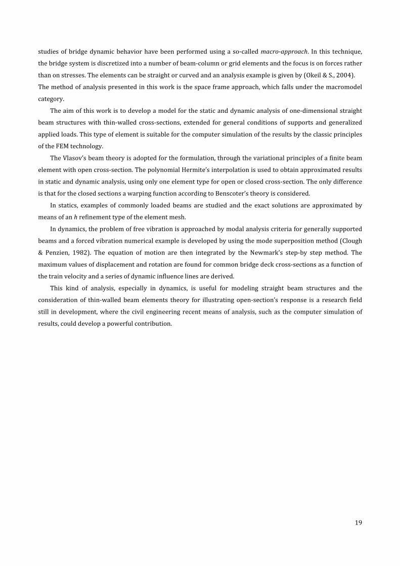
The axial displacement �$ is obtained from the linear combination of four components, one from a rigid body

translation % (figure 3.3), two from rotation around lines such as the � and - axis in the cross-section and finally

one from warping.

The rotations of the cross-section, &� and &� , associated with the beam bending can be obtained according to

the Bernoulli hypothesis as follows

&� = ��′ (3.3)

&� = −��′ (3.4)

x

y

θ y

ux

x

y

ux

ηy=yc

z=zc

y=yc

ux

z=zc

(x,y) (x,y)

xx

(x,z)

ux

z z(x,z)

η

θ z

ξ y

ξ z

Figure 3.3- Axial displacements of an I-Beam due to axial effect and bending for planes (x,y) and (x,z).

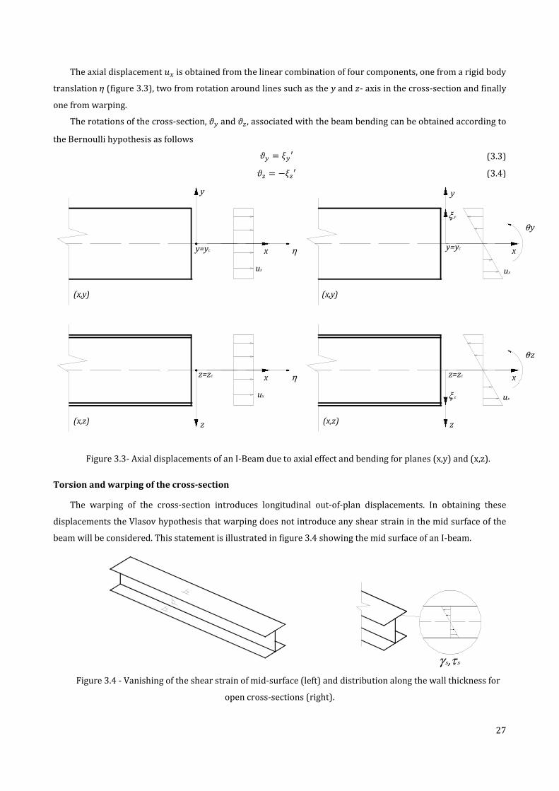
Torsion and warping of the cross-section

The warping of the cross-section introduces longitudinal out-of-plan displacements. In obtaining these

displacements the Vlasov hypothesis that warping does not introduce any shear strain in the mid surface of the

beam will be considered. This statement is illustrated in figure 3.4 showing the mid surface of an I-beam.

γ τ

Figure 3.4 - Vanishing of the shear strain of mid-surface (left) and distribution along the wall thickness for

open cross-sections (right).

28

This condition does not interfere with Saint Venant homogeneous torsion problem, that assume linear

variation of stress *+ and strain ,+ over the thickness (figure 3.4).

The vanishing shear strain condition in the mid-surface of the beam enables a direct determination of the

cross-section warping function. When cross-sections twist, they are assumed to remain non-deformed in their

own plane, so their displacements can be described by the axial component �$(-, �) and a rotation �(�) around a

point P. The position on the centerline is described by the arc length-, shown in figure 3.5, and the center of

rotation is assumed to be known.

P

h(s)

s

us(x,s)

ϕ( x )

Figure 3.5 - Rotation of open cross-section.

The in-plane displacement �+ along the tangent at - can be written as

�+(-, �) = ℎ(-)�(�) (3.5)

The condition of no shear deformation is

,(-, �) = 0�+0� + 0�$0- = 0 (3.6)

That yields, substituting �+ ,followed by integration with respect to -

�$(-, �) = − 0�(�)0� 2 ℎ(-)+ 3- (3.7)

Starting from the equation (3.7) a new quantity can be defined as sectorial coordinate and is

2 ℎ(-)+ 3- = 4(-) (3.8)

The interpretation of this function is discussed in the next two sections for an open and a closed cross-

section, respectively.

Sectorial coordinate of an open cross-section

The sectorial coordinate 5 ℎ(-)+ 3- = 4(-) defined by the equation (3.8) has a geometric interpretation for

an open section. As shown in figure 3.6 it represents twice the area swept by a line from the center of rotation �

to the generic point - on the midline of the section wall. Upon the integration on the total length of the arc 4(-) = 26+.

29

P

h(s)

ϕ(x)

us(x,s)

ds

A(s)

Figure 3.6 – Geometric interpretation of the sectorial coordinate. Later will be discussed how to calculate the position of the center of rotation by means of its particular

properties with respect to bending and axial displacements.

Sectorial coordinate for a closed thin-walled section

Vlasov theory is stated as applicable for closed cross-sections by combining the assumption of neglecting

shear warping at midwalls for the calculation of profile warping function with Benscoter independent warping

degree of freedom. Usually for a closed section the integral of the equation (3.8), extended to the entire perimeter,

is most known in the following form

7 ℎ(-) 3- = 4(-) = 26+ = Ω (3.9)

The shear distortion of the equation (3.6), if calculated for a closed section yields

,(-, �) = 0�+0� + 0�$0- = ,9 (3.10)

The value of the shear distorsion is given by Bredt’s formulae and gives

,9 = �Ω: (3.11)

Substituting equations (3.5), (3.7) and (3.11) in equation (3.10) follows that

�$(� = -) = �$(� = 0) + 2 �Ω: 3-+; − �< 2 ℎ(-)3-+

; (3.12)

If the totality of the closed perimeter is considered in the integrals, it leads to

7 �Ω: 3- = �< 7 ℎ(-)3- = �<Ω (3.13)

Where Ω has been defined in (3.9). From(3.13) the rate of twist and the torsional stiffness modulus can be

obtained as follows

�< = �:= (3.14)

= = Ω>∮ @+9 (3.15)

Now a new sectorial coordinate can be calculated from (3.12) that leads to

�$(� = -) = −�<4(-) (3.16)

30

where 4(-) is the coordinate defined as

�(-) = 4(-) − Ω∮ @+9 2 3-+; + AB (3.17)

in which AB can be obtained imposing as zero the axial virtual work ∮ �(-) (-)3- = 0. Note that this coordinate

has been defined for the shear center but the same formulae obtained in the next are valid, because of the

validity of the Vlasov theory.

Total axial displacements of the cross section

With all the contributions of the general displacements, the axial displacement of a thin-walled beam of open

cross section is represented in the form

�$(-, �) = %(�) − (� − �C)��<(�) − ( − C)��<(�) − �(-)�<(�) (3.18)

The variation of �$ over the section is described by the classical Euler-Bernoulli assumption by means of %(�), ��(�), ��(�), while the last term, composed by �(�), represents the displacement due to the warping of

section. The equation (3.18) can be considered as an axial effect of the classic beam theory in which torsion is

incorporated in a systematic way, including its non-homogeneous part.

Tangential shear strain over the cross-section

The complete form of the warping function can be found by imposing the shear strain value at the mid-

surface of the beam wall. The displacement components of the equations (3.18) have been derived directly from

the assumption of Vlasov’s theory and implying

,� = 0��0� + 0�$0� = D−( − �) − 0�0� E �< = 0 ⟹ 0�0� = −( − �) (3.19)

,� = 0��0� + 0�$0 = G(� − ��) − 0�0 H �< = 0 ⇒ 0�0 = (� − ��) (3.20)

Taking into account the definition of the tangent vector as

J = KB>L=M@�@+@�@+N (3.21)

the displacement derivatives relatively to the arc length - can now be calculated as follows

0�0- = 0�0� B + 0�0 > = 0�0� 3�3- + 0�0 33- = −( − �) 3�3- + (� − ��) 33-

(3.22)

where the components B, > describe the tangent vector in the plane as shown in equation (3.21).

Considering the definition of the normal to the thin wall as

O = KPBP>L=M− @�@+ @�@+N

(3.23)

the projection ℎ of the vector of coordinates Q( − �), (� − ��)R on the local normal (figure 3.7) can be identified

in the equation (3.22). The relations obtained can be written as follows

31

0�0- = ℎ(-) (3.24)

0�0P = 0�0� PB + 0�0 P> = 0�0 3�3- − 0�0� 33- = (� − ��) 3�3- + ( − �) 33- (3.25)

The parameter ℎ+identified in figure 3.7 is defined by the equation (3.25). In fact it leads to

ℎ+ = (� − ��) 3�3- + ( − �) 33- = 0�0P (3.26) which represents a linear variation of � across the wall thickness, i.e.

�(-, P) = �ST;(-) + ℎ+(-)P (3.27)

P

h(s)

s

ϕ(x)

(dy/ds,dz/ds)

(y,z)

(dz/ds,-dy/ds)

hs(s)

Figure 3.7 – Geometric interpretation of h(s) and hs(s).

The distribution of the tangential shear strain component over the wall thickness can then be obtained as

follows

, =0�+0� +

0�$0- =00� ((ℎ + P)�) +

00- (−��<) = 2P�< (3.28)

which corresponds to the linear variation of the Saint Venant shear strain for open thin-walled sections.

Axial strain over the cross-section

The strain component U along the beam axis is obtained from the derivative of the axial displacement (3.18)

as follows

U = %<(�) − (� − �C)��<<(�) − ( − C)��<<(�) − �(-)�<<(�) (3.29)

3.1.2. Potential energy formulation

The potential energy is defined by two parts, the strain energy and the external work produced by the load.

Two strain components are present in the current analysis, the normal axial strain U and the Saint Venant shear

strain ,. By applying Hooke’s law is possible to obtain the corresponding axial and shear stresses

Axial stress: V = WU (3.30) Shear stress: * = :, (3.31) where W is the module of elasticity and : is the shear modulus of the prescribed material, given by : = k>(Blm). These two quantities are assumed to be constant along the bar length. The elastic strain energy density per unit volume is obtained from the two components as follows q = B> WU> + B> :,> (3.32)

The load is given in terms of volume forces, so the external work per unit volume can be expressed as follows

32

r = s$�$ + s��� + s��� = t ∙ v (3.33)

being t = ws$s�s� x the vector of volume forces and v = w�$���� x the displacements vector considered.

Axial strain energy per unit length

The strain energy per unit length is obtained by integration of the equation (3.32) over the cross section area. The integration of the axial strain (3.29) gives the contribution

12 2 WU>z 36 = 12 W 2 {%′(�) − (� − �C)��<<(�) − ( − C)��<<(�) − �(-)�<<(�)|>z 36 =

= 12 W{%< −��<< −��<< −�<<| }~~~� 6 ���� ��� �� ����� ����� ����� ��� ��� ������ ������

��}~~~� %<−��<<−��<<−�<< ���

�� (3.34)

This is the expression of the quadratic and symmetric mathematical energy density after integration over the transverse area. The vector {%< −��<< −��<< −�<<| represents the generalized strains, including axial, flexural and warping components. The terms in the matrix are obtained from integration over the area and represent the cross-section geometrical parameters. It is useful to specify that all the sectorial moments refers to the point P, which is generic. All these quantities are represented in the table 3.1. Tangential strain energy per unit length

The Saint Venant shear strain energy contribution is obtained by the following integration

12 2 :,> 36 = 12 �<:=�< (3.35)

In table 3.1 are listed all the geometrical properties of the cross-sections.

33

Table 3.1 - Cross-Section parameters.

Quantities Open Section Closed Section

Area: 6 = 2 36z 6 = 7 36z

Static moment:

�� = 2 (� − �C)z 36 �� = 7 (� − �C)z 36

�� = 2 ( − C)z 36 �� = 7 ( − C)z 36

Moments of inertia:

�� = 2 (� − �C)>z 36 �� = 7 (� − �C)>z 36

�� = 2 ( − C) > z 36 �� = 7 ( − C) > z 36 ��� = 2 ( − C) (� − �C) z 36 = ��� ��� = 7 ( − C) (� − �C) z 36 = ���

Sectorial moments:

�� = 2 �(-)36z �� = 7 4(-)36z

��� = 2 (� − �C) �(-)z 36 ��� = 7 (� − �C) 4(-)z 36 ��� = 2 ( − C) �(-)z 36 ��� = 7 ( − C) 4(-)z 36

��� = 2 �(-)>z 36 ��� = 7 4(-)>z 36

Torsion parameter: = = 13 2 � 3- = = Ω>∮ @+9

External work per unit length

Integrating the equation (3.33) over the cross-section area the following expression is obtained

2 �s$�$ + s��� + s����36z = �$% + ���� + ���� + ��� − ���<� − ���<� − ��< (3.36)

where the load is considerate in terms of volume forces by means of s$ , s� , s� . Surface tractions and

concentrated loads can be considered as limiting forms of volume forces.

All the beam loads are defined in table 3.2. Notice that for each generalized displacement %, �� , �� , �, �<� , �<� , �< there is a beam load, as the boundary conditions imposed. This 7 displacement components

34

are thee degrees of freedom of thin-walled beam elements, so warping can be considered as an aditional d.o.f. to

the 6 of a simply one-dimensional beam in space.

Table 3.2 – Beam loads per unit length.

Quantities Open Section Closed Section Axial load: �$ = 2 s$36z �$ = 7 s$36z

Transverse load:

�� = 2 s�36z �� = 7 s�36z

�� = 2 s�36z �� = 7 s�36z

Bending moment loads:

�� = 2 s$(� − �C)z 36 �� = 7 s$(� − �C)z 36

�� = 2 s$( − C)z 36 �� = 7 s$( − C)z 36 Torsion moment load: �� = 2 s�(� − ��) − s�( − �)z 36 �� = 7 s�(� − ��) − s�( − �)z 36

Bimoment load: � = 2 s$z �(-)36 � = 7 s$z 4(-)36

Total potential energy

The total potential energy of the beam element can now be defined by the total quantity � or by the unit

length energy �, after the integration over the cross-section area. The strain energy component is composed by

quadratic terms, while the applied load part is represented by linear terms. Thus, the following expressions are

obtained ���� s��P��� �P����: � = 2 (q − r)3�� = 2 D12 WU> + 12 :,> − (s$�$ + s��� + s���)E 3�� (3.37)

���P��� �P���� s�� �P� ��P�ℎ: � = 2 � �%, %<, �, �<, �<<, ��, ��, �<� , �<�, �<<� , �<<�  3�¡ (3.38)

where the functional � is defined by

35

� �%, %<, �, �<, �<<, �� , �� , �<� , �<�, �<<� , �<<�  =

= 12 W(%<6%< − %<���<<� − %<���<<� − %<���<< −�<<���%< + �<<����<<� + �<<�����<<� + �<<�����<< −�<<���%< + �<<�����<<� + �<<����<<� + �<<�����<< −�<<��%< + �<<����<<� + �<<����<<� + �<<����<<)

+ 12 �<:=�< − ��$% + ���� + ���� + ��� − ���<� − ���<� − ��< 

(3.39)

In the next part will be specified a suitable choice of the elastic center (�C , �C) and of the center of

rotation (�� , ��) in order to obtain considerable simplifications of the equation (3.39) in coupling terms outside

the diagonal of matrix of (3.34).

3.1.3. Elastic center and shear center

The coupled terms that appear in the energy density � take into account the contribution of the different

generalized displacements and represent the coupling between axial effect, bending and torsion, which implies,

for example, that a solution involving flexural displacements will also activate torsion and extension of the beam.

The coupling between extension and bending is eliminated for �� , �� = 0, while coupled effects in extension and

bending with respect to torsion displacements are cancelled if ��, ��� , ��� = 0.

The elimination of the static moments of Table 3.1 follows from the choice of the point (�C , C) as defined

below

�C = 16 2 � 36z (3.40)

C = 16 2 36z (3.41)

This defines the elastic center of the cross-section for homogeneous cross-section of the beam. In a similar way, the condition ��, ���, ��� = 0 implies no bending or axial effect when the cross-section twists. The shear center is defined by the property ��� , ��� = 0, while �� = 0 is satisfied by including a suitable constant in the definition of the sectorial coordinate (3.8). The coordinates (�¢, ¢) of this point will be defined neglecting the shear strain at the mid surface and evaluating the difference between sectorial coordinates �¢ and �� as follows

0(�¢ − ��)0� = −(� − ¢) (3.42)

0(�¢ − ��)0 = (�� − �¢) (3.43)

being (�� , �) the coordinates of the generic point of rotation � that define the sectorial coordinate �� .

36

The assumption have been done considering open sections. For compact and hollow section the distortion is present because of the elastic shearing of the cross section and has to be accounted for its effect in the warping parameter. In the next an adapted warping coordinate 4(-) will be considered for closed sections according to (Benscoter, 1954). Integration of the relations (3.42) and (3.43) gives the expression of �¢

�¢(-) = ��(-) + (¢ − �)(� − �C) − (�¢ − ��)( − C) − A (3.44) where the unknown constant A is obtained by substitution of the expression of �¢ into the condition ��© = 0. The value of the constant is A = 16 2 ��(-)z 36 = ��ª6 (3.45)

The expression of �¢(-) can now be substituted in the orthogonality conditions ��� , ��� = 0, allowing to

obtain the following equations

���ª + (¢ − �)�� − (�¢ − ��)��� = 0 (3.46)

���ª + (¢ − �)��� − (�¢ − ��)�� = 0 (3.47)

Considering the equations (3.46) and (3.47) the coordinates of the shear center (�¢, ¢) are obtained as

follows

K�¢¢L = K���L + 1���� − ���> « �� ������ �� ¬ « ���ª−���ª¬ (3.48)

The torsion problem is uncoupled between the axial effect and the bending of the beam when (�C , C) are the

coordinates of the elastic center and (�¢ , ¢) define the shear center. This uncoupling is convenient from the

point of view of analysis and useful to describe the non-homogeneous torsion mechanics.

Transformation of sectorial coordinates

The warping coefficient of the generic cross-section may be obtained either from integration of the sectorial

coordinate �¢ or by transformation of the sectorial coordinate in relation to the generic sectorial coordinate �� .

The substitution of (3.44) and (3.45) in the definition of ���¢ leads to the following transformation formula:

���¢ = ���� − ���>6 + Q�¢ − �� ¢ − �R « �� −���−��� �� ¬ K�¢ − ��¢ − � L (3.49)

Notice that the sectorial parameter for a generic point � of the cross-section is always more than ���¢ , which

means that the sectorial parameter corresponding to the shear center is the principal sectorial coordinate. 3.1.4. Kinetic energy formulation

The beam kinetic energy is defined as follows

� = 2 12 v­ ®¯v­ 3�� (3.50)

being the corresponding energy per unit volume defined as

12 v­ ®¯v­ = 12 ¯(�$­ > + ��­ > + ��­ >) (3.51)

37

The general expression per unit length is obtained by integration of (3.51) and substituting the velocities �­ $,�­ �,�­ � from their definition in section 3.1.1. The dots define integration over the time and ¯ Q°�/��R is the

mass per unit volume of the material.

Axial kinematic energy component

The axial component of the kinetic energy is defined as follows

12 ¯��$­ >� = 12 ¯ �%­ − (� − �C)�­�< − ( − C)�­�< − �(-)�­ < >

= 12 ¯(%­> − %­(� − �C)�­�< − %­( − C)�­�< − %­�(-)�­ < −(� − �C)�­�<%­ + D(� − �C)�­�<E> + (� − �C)( − C)�­�<�­�< + (� − �C)�(-)�­�<�­ < −( − C)�­�<%­ + ( − C)(� − �C)�­�<�­�< + D( − C)�­�<E> + ( − C)�(-)�­�<�­ <

−�(-)�̇′%̇ + �(-)(� − �A)�̇′�̇�′ + �(-)( − A)�̇′�̇′ + (�(-)�̇′)2)

(3.52)

The axial kinetic energy is composed by the contribution of extension, bending and torsion given the warping

of the cross-section.

In-plane kinematic energy components

Kinematic quantities ��­ , ��­ also generate kinetic energy contribution. If eq.(3.1) and eq.(3.2) are considered

is possible to obtain 12 ¯���­ > + ��­ >� =12 ¯ ���­ > − 2��­ ( − �)�­ + �( − �)�­ �> + ��­ > + 2��­ (� − y�)�­ + �(� − y�)�­ �>  (3.53)

In this part of the energy expression Saint Venant kinetic energy of shear is taken into account by the terms

involving rigid rotation around the generic point P.

Total kinetic energy per unit length

The integration over the cross-section of the eq.(3.52) and (3.53) leads to the energy ± per unit length of the

beam, which allows to obtain the beam kinetic energy written as follows:

� = 2 ±(%­ , ��­ , �� ,­ �­ , �­�<, �­�<, �­ <)3�¡; (3.54)

where

38

± �%­ , ��­ , �� ,­ �­ , �­�<, �­�<, �­ <  = 12 ¯(6%­> − ��%­�­�< − ��%­�­�< − ��%­�­ < −���­�<%­ + ���­�<> + ����­�<�­�< + ����­�<�­ < −���­�<%­ + ����­�<�­�< + ���­�<> + ����­�<�­ < −���̇′%̇ + ����̇′�̇�′ + ���̇′�̇′ + ����̇′2

+6��­ > − 2��­ ����­ + ����­ >

+6��­ > + 2��­ ����­ + ����­ >)

(3.55)

Notice that in (3.55) all the coupling terms are considered. The geometric moments of inertia refer to the

same generic point �. The uncoupling in terms of the kinetic energy defined in (3.55) is similar to the static case

and corresponds to in-plane twist around the shear center while bending and axial effect are considered in

relation to the elastic center.

3.2. Static analysis

In 3.1 the potential energy of a thin-walled beam of general cross-section was formulated and two particular

points have been identified in the cross-section plan, the elastic center and the shear center. When the

deformation of a beam is described considering these two points, axial effect, bending and torsion of the beam

are uncoupled. In the following this uncoupled expression for the deformation field is adopted, in order to

simplify the expression of equilibrium equations.

The equilibrium equations and corresponding static boundary conditions are derived in 3.2.1 for extension,

bending and torsion considering the potential energy of the beam.

Solution of simple torsion problems are described for various load types and depending from the cross-

section shape. The influence of warping is defined in terms of section stiffness showing differences between

closed and open sections.

3.2.1. Equilibrium and stresses

The potential energy density per unit length is expressed in terms of the generalized displacements and their

derivatives as already specified by the function � �%, %<, �, �<, �<<, �� , �� , �<� , �<� , �<<� , �<<� . In eq.(3.39) a function

of functions is called a functional, and the approach that will be used for developing the equilibrium equations is

based on variational principles. The displacement functions will be obtained by examining how the functional

varies as these functions change, taking into account infinitesimal variations. The solution for each generalized

displacement satisfies the kinematic boundary conditions and gives the minimum value of � �%, %<, �, �<, �<<, �� , �� , �<� , �<�, �<<� , �<<� . This is called the theorem of minimum potential energy and allows to

obtain a set of differential equations, which correspond to the solution of the equilibrium in their strong form.

The potential energy will refer to the elastic center (�C , C) and to the shear center (�¢ , ¢) and is presented

in its uncoupled form. Therefore, axial effect, bending and torsion can be treated separately, and all the coupling

geometric quantities will vanish.

39

Axial effect

The generalized displacement %(�) describe the axial extension of the beam. The associated potential energy

is given by

�(%, %<) = 2 D12 %<W6%< − �$%E 3�¡; (3.56)

The corresponding variation in the functional is denoted by ²�(%), which is defined by

²�(%) = ��%(�) + ²%(�)� − ��%(�)� = 2 (%<W6²%< − �$²%)3�¡; + 2 12 ²%<W6²%<3�¡

; (3.57)

The third term is a second order term and can be neglected because ²% is small. Thus the condition of

minimum potential energy implies that ²�(%) = 0, allowing to derive the following equation

2 (%<W6²%< − �$²%)3�¡; = 0 (3.58)

At the minimum of �(%) the first variation of the functional must vanish for the arbitrary variations ²%(�)

that satisfy the kinematic boundary conditions. This is expressed as ²�(%)=0. The integral (3.58) is reformulated

via integration by parts, whereby the derivative ²%< is integrated, and gives

²�(%) = Q%<W6 ²%R;¡ − 2 ²%Q(%<W6)< + �$R3�¡; = 0 (3.59)

The first term in (3.59) is the boundary condition, defined for each end of the beam. The boundary forces

satisfies the global equilibrium of the beam and thus Q%<W6 ²%R;¡ = 0. In the integral, for arbitrary variations ²%(�) the term in brackets must vanish everywhere in order to verify the vanishing of ²�. This allows to obtain

the differential equation that corresponds to the extension equilibrium

33� DW6 3%3�E + �$ = 0 (3.60)

The boundary terms are in the form of a product of the variation of the axial displacement ²% and a factor

easily identified as the normal force

³ = 2 V$z 36 = W6 3%3� (3.61)

When the normal force given by (3.61) is introduced into (3.60), the equilibrium equation for the extension

is

3³3� + �� = 0 (3.62)

This is the equilibrium equation for the beam extension problem, where the axial stiffness of the beam W6 is

supposed to be constant along the beam axis.

Bending

The bending problem is treated with the same approach. The only differences are that in this case there are

two displacement components (�� , ��) and that also their second derivatives must be taken into account in the

definition of the strain energy.

40

The associated potential energy is

���´ , �´<, �´<<� = 2 D12 �<<µW�µ¶�<<¶ − (�µ�µ − �µ�<µ)E 3�¡; (3.63)

The use of the subscript , in eq.(3.63) is to indicate the two components (�� , ��) and to avoid any relation to

the subscripts and �. The repeated subscripts and � imply summation over = �, and � = �, . This form

is complete for the bending problem: simplifications of potential expression occur if the �, axis are the principal

axes with origin at the elastic center.

The first variation of ���´ , �´<, �´<<� is the linear part of the difference � ��´(�) + ²�´(�)  − � ��´(�)  and

can be written as follows

²���´� = 2 �²�<<µW�µ¶�<<¶ − (−�µ²�<µ + �µ²�µ) ¡; 3� (3.64)

The first term is integrated twice by parts and the second term is integrated once. The result is the following

²���´� = K²�<µ �W�µ¶�<<¶  − ²�µ �W�µ¶�<<¶ < + ²�µ�µL;¡ + 2 ²�µ ��W�µ¶�<<¶ << − �µ< − �µ ¡

; 3� (3.65)

The stationarity condition imposes ²���´� = 0 and implies that the factor ²�´ = (²�� , ²��) must vanish

identically over the length of the beam, therefore:

323�2 ( W� � 32��3�2 ) − 3� 3� − � = 0, = �, (3.66)

This differential equation represents the solution for the flexural problem in the principal direction. Note

that eq. (3.66) is a vector equation with two components.

In this case the boundary terms in eq. (3.65) identify the bending moments �µ and the shear forces �µ , with

their contribution to the virtual work by the rotations −²�<µ and the displacements ²�µ , respectively. Thus the

first boundary term identifies the bending moments

�µ = −W�µ¶ 3>�¶3�> , = �, (3.67)

while the second and third boundary terms identify the shear forces

�µ = − 33� ·W�µ¶ 3>�¶3�> ¸ + �µ , = �, (3.68)

Substituting the eq.(3.67) in the eq.(3.68) and then eq.(3.68) in eq.(3.66) the equilibrium equations of the

bending problem are expressed in terms of statics as

�µ = 3�µ3� + �µ , = �, (3.69)

3�µ3� + �µ = 0, = �, (3.70)

Torsion

For the formulation of the equilibrium equations the torsion problem is described in terms of the angle of

twist �(�) around the axis of the cross-section shear centers (�¢ , ¢). The potential energy expression leads to

41

�(�, �<, �<<) = 5 B> ��<<W����<< + �<:=�< − ���� − ��<�  3�¡; (3.71)

being the first variation of �(�)written as follows

²�(�) = 5 �²�<<W����<< + ²�<:=�< + �²�< − ��²��3�¡; (3.72)

After the integration by parts the first variation takes the form

²�(�) = Q²�<(W����<<) − ²�(W����<<)< + ²�:=�< + ²��R;¡ + 5 ²��(W����<<)<< − (:=�<)< − �< − ���3�¡; (3.73)

The stationary condition implies the vanishing of the integral term in brackets of the equation (3.73) for

arbitrary values of ²�(�). This gives the differential equation of torsion

3>3�> ·W��� 3>�3�> ¸ − 33� D:= 3�3�E − 3�3� − �� = 0 (3.74)

The boundary term in (3.73) multiplied by −²� <identifies the bimoment as

�� = −W��� 3>�3�> (3.75)

The torsion moment is obtained by taking into account all the terms in eq.(3.73) that correspond to the

virtual work when multiplied by ²�

� = − 33� ·W��� 3>�3�> ¸ + := 3�3� + � (3.76)

Three contributions constitute the torsion moment: the warping moment, the Saint Venant moment and the

externally applied distributed bimoment �:

r��s�P� ��-��P: �� = 3��3� = − 33� ·W��� 3>�3�> ¸ (3.77)

���P ��P�P ��-��P: �¹ = := 3�3� (3.78)

Finally, substituting eq.(3.77) and eq.(3.78) in eq.(3.76) the torsion moment is

� = �� + �¹ + � (3.79)

Substituting the eq.(3.76) in eq.(3.74) the second equilibrium equation for torsion is obtained

3�3� + �� = 0 (3.80)

Boundary conditions

The seven equilibrium equations have been defined considering extension, bending and torsion within the

context of the theory of thin-walled beams. Seven boundary conditions, corresponding to the number of the

degrees of freedom, are required for each end point of the beam for solving the static problem.

There are two basic forms of the boundary conditions. A kinematic boundary condition assigns a prescribed

value to one of the seven general displacements. Alternatively a static boundary condition allows an arbitrary

value of displacement but the corresponding static quantity must equal an external load at the same point.

42

In table 3.3 equilibrium equations obtained and boundary conditions quantities are shown for extension,

bending and torsion.

Table 3.3 – Equilibrium equations and boundary conditions.

Equation Kinematic Static

Extension 3³3� + �� = 0 % ³

Bending

�� = 3��3� + �� 3��3� + �� = 0

�� , −�′� �� , ��

�� = 3��3� + �� 3��3� + �� = 0

� , −�′ �� , ��

Torsion

� = �� + �¹ + � 3�3� + �� = 0 � , �< �, ��

Note that for non-symmetrical cross-sections the elastic center axis and shear center axis could not coincide.

This means that the differential governing equations mentioned above are referred to two different �-axis. For

example, in a C cross-section all the displacements and forces are illustrated in figure 3.8 and figure 3.9 where is

shown that only the choice of two different axis serves to uncoupling the bending and the extension of the beam

from its torsion behavior.

43

Elastic center axis (yC,zC)

Shear center axis (ya,za)

y θ z

θ y

ξ y

ξz

η

x ϕ

z

ϕ '

Figure 3.8 – Generalized displacements of a C cross-section beam.

V y

M z

V z

M y

NTM ω

Elastic center axis (y C,zC)

Shear center axis (y a,za)

Figure 3.9 – Forces in a C cross-section beam.

3.2.3. Basic load cases

With the appropriate axes adopted for the decoupling of the equilibrium equations, extension, bending and

torsion can be treated independently. The solutions techniques for Euler-Bernoulli theory applied on beams are

assumed to be well known. Thus, only the non-homogeneous torsion problem is treated in this section and basic

load cases are presented.

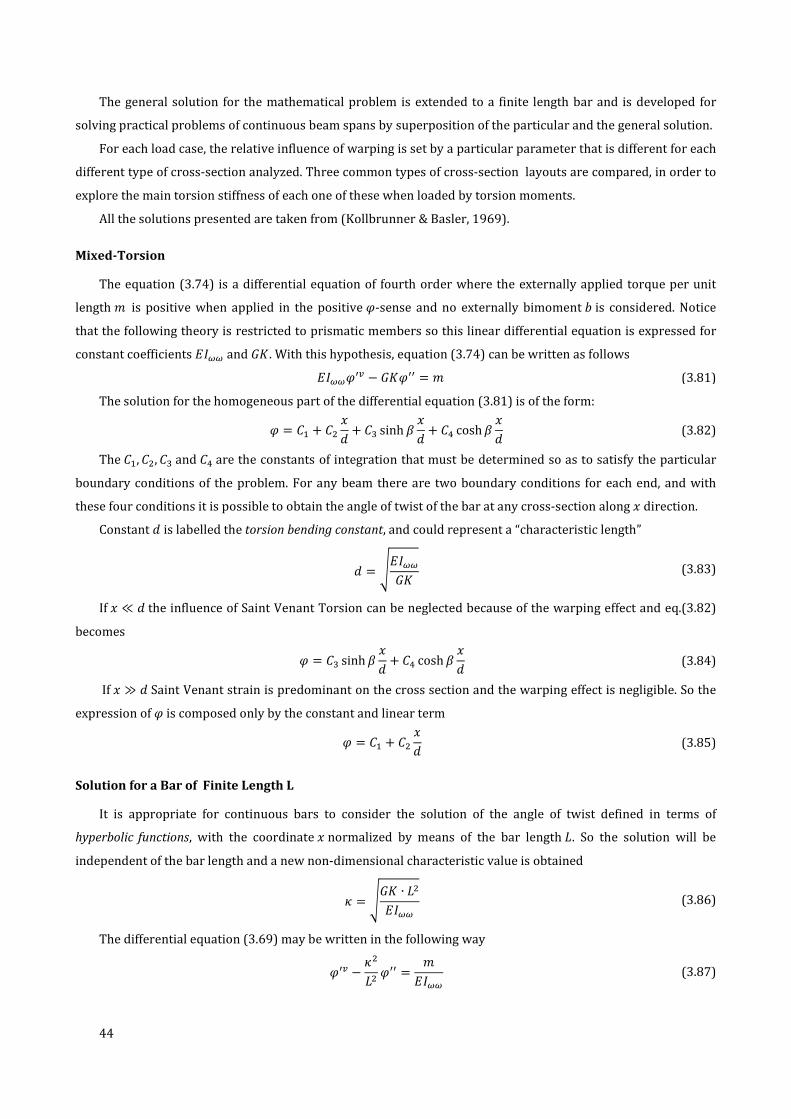
44

The general solution for the mathematical problem is extended to a finite length bar and is developed for

solving practical problems of continuous beam spans by superposition of the particular and the general solution.

For each load case, the relative influence of warping is set by a particular parameter that is different for each

different type of cross-section analyzed. Three common types of cross-section layouts are compared, in order to

explore the main torsion stiffness of each one of these when loaded by torsion moments.

All the solutions presented are taken from (Kollbrunner & Basler, 1969).

Mixed-Torsion

The equation (3.74) is a differential equation of fourth order where the externally applied torque per unit

length � is positive when applied in the positive �-sense and no externally bimoment � is considered. Notice

that the following theory is restricted to prismatic members so this linear differential equation is expressed for

constant coefficients W��� and :=. With this hypothesis, equation (3.74) can be written as follows

W����<¼ − :=�<< = � (3.81)

The solution for the homogeneous part of the differential equation (3.81) is of the form:

� = ±B + ±> �3 + ±� sinh � �3 + ±½ cosh � �3 (3.82)

The ±B, ±>, ±� and ±½ are the constants of integration that must be determined so as to satisfy the particular

boundary conditions of the problem. For any beam there are two boundary conditions for each end, and with

these four conditions it is possible to obtain the angle of twist of the bar at any cross-section along � direction.

Constant 3 is labelled the torsion bending constant, and could represent a “characteristic length”

3 = ¾W���:= (3.83)

If � ≪ 3 the influence of Saint Venant Torsion can be neglected because of the warping effect and eq.(3.82)

becomes

� = ±� sinh � �3 + ±½ cosh � �3 (3.84)

If � ≫ 3 Saint Venant strain is predominant on the cross section and the warping effect is negligible. So the

expression of � is composed only by the constant and linear term

� = ±B + ±> �3 (3.85)

Solution for a Bar of Finite Length L

It is appropriate for continuous bars to consider the solution of the angle of twist defined in terms of

hyperbolic functions, with the coordinate � normalized by means of the bar length �. So the solution will be

independent of the bar length and a new non-dimensional characteristic value is obtained

� = ¾:= ∙ �>W��� (3.86)

The differential equation (3.69) may be written in the following way

�<¼ − �>�> �<< = �W��� (3.87)

45

Now it is useful to represent the solution in terms of a new non-dimensional and normalized coordinate � = �/�.

Considering a particular solution �] of the differential equation for each load case, the strain and the stresses

could be written as follows

6P��� �Á Â�- � = ±B + ±>� + ±� sinh �� + ±½ cosh �� + �à (3.88)

6P��� �Á Â�- s�� �P� ��P�ℎ �′ = ±> B¡ + ±� Ä¡ sinh �� + ±½ Ä¡ cosh �� + �à ′ (3.89)

r��s�P� ����P �� = −:=(±� sinh �� + ±½ cosh ��) − WI���Ã′′ (3.90)

���-��P�� ����P � = := �ÅÆ¡ + �à ′  − WI���Ã′′′ (3.91)

Beam cross-sections

Solutions are obtained for three different sections, as shown in Table 3.4, where C is the elastic center and A

the shear center

Table 3.4 - Cross-section layouts and position of the elastic and shear center.

h

b

tf

tf

twC=A

b

tw

tf

hCA

h

b

tf

tw

tf

C=A

�[��] 100 100 170 ℎ[��] 360 360 360 Ç[��] 14 14 8 È[��] 14 14 12.7

Admitting a beam length of L=2m, a different value of the constant � is obtained for each of the cross-

sections analyzed:

• Closed hollow section: b = 100mm, h = 360mm, t = tw = tf = 14mm, �ÉÊËËÊÇ +ÌC. = 19.89 .

• Channel cross Section: b = 100mm, h = 360mm, t= tw= tf = 14mm, �Å +ÌC. = 1.5. • I cross Section: b = bf1 = bf2 = 170mm, tf = 12.7mm, tw = 8mm, �Î +ÌC. = 1.19.

The constant � is an index of the cross-section behavior with respect to the torsional stiffness. As � ≫ 1 for

the closed hollow section, this means that the torsional response of this cross-section tends to pure Saint-Venant

Torsion response. For the channel and I-section = 3/� ≈ 1 , both warping torsion and Saint Venant torsion have

to be taken into account. The difference between a C and I-section is that the first one is mono-symmetric and the

shear center does not coincide with the elastic center. In this case when a bending external load is acting on the

beam the effect of torsion and bending are coupled. In fact for a C-section the boundary conditions for torsion are

referred to the shear center axis. For I-section, the problem of torsion and bending could even be solved as

uncoupled because of the coincidence of these two axes.

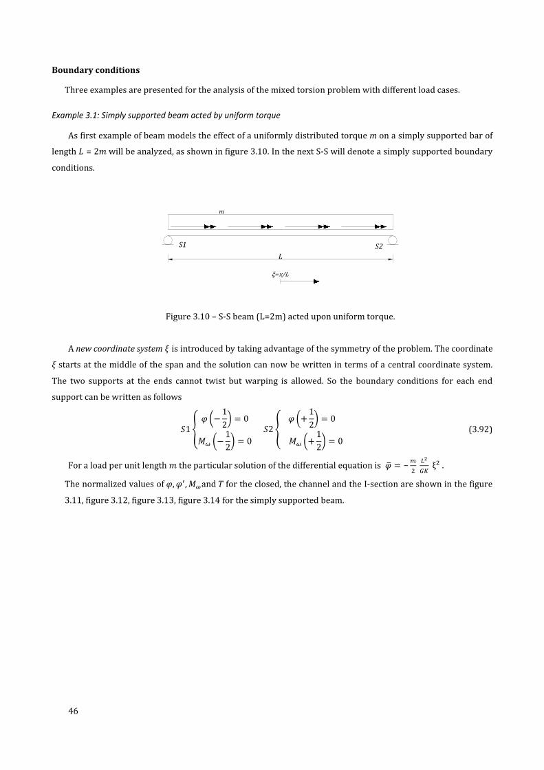
46

Boundary conditions

Three examples are presented for the analysis of the mixed torsion problem with different load cases.

Example 3.1: Simply supported beam acted by uniform torque

As first example of beam models the effect of a uniformly distributed torque m on a simply supported bar of

length � = 2� will be analyzed, as shown in figure 3.10. In the next S-S will denote a simply supported boundary

conditions.

L

m

ξ=x/LS1 S2

Figure 3.10 – S-S beam (L=2m) acted upon uniform torque.

A new coordinate system � is introduced by taking advantage of the symmetry of the problem. The coordinate � starts at the middle of the span and the solution can now be written in terms of a central coordinate system.

The two supports at the ends cannot twist but warping is allowed. So the boundary conditions for each end

support can be written as follows

�1 Ñ � D− 12E = 0�� D− 12E = 0Ò �2 Ñ � D+ 12E = 0

�� D+ 12E = 0 Ò (3.92)

For a load per unit length � the particular solution of the differential equation is �à = −Ó> ¡ÆÔÕ ξ> .

The normalized values of �, �<, ��and � for the closed, the channel and the I-section are shown in the figure

3.11, figure 3.12, figure 3.13, figure 3.14 for the simply supported beam.

47

Figure 3.11 - � value of a S-S2 beam acted by uniform torque (analytical solution).

Figure 3.12 – �′ value of a S-S beam acted by uniform torque (analytical solution).

Figure 3.13 - �� of a S-S beam acted by uniform torque (analytical solution).

2 Simply Supported

-0.5 -0.4 -0.3 -0.2 -0.1 0 0.1 0.2 0.3 0.4 0.5

-0.1

0

0.1

0.2

ξ

φ*

GK

/mL2

Twist angle normalized

C I Hollow

-0.5 -0.4 -0.3 -0.2 -0.1 0 0.1 0.2 0.3 0.4 0.5

-0.5

0

0.5

ξ

φ'*

GK

/mL

C I Hollow

-0.5 -0.4 -0.3 -0.2 -0.1 0 0.1 0.2 0.3 0.4 0.5

0

0.05

0.1

0.15

0.2

ξ

Mw

/mL2

Mw normalized

C I Hollow

48

Figure 3.14 – Distribution of the torsion �¹ and � of a S-S beam acted by uniform torque (analytical solution).

The normalized twist is proportional to the Saint Venant torsional stiffness := and, as expectable, the twist

of the hollow section achieves values much higher at midspan, while the torsion angle between the two open-

sections is of the same order of magnitude (figure 3.11). Note that the first derivative of the twist angle is

proportional to the Saint Venant torsion contribution: this means that the torsion moment � of the hollow beam

is mainly composed by �¹ (figure 3.12 and figure 3.14). On the other hand, the warping of the open sections gives

higher values of the warping moments at the beam supports (figure 3.13), and the main torsion contribution of

the I and C-beam is the ��.

Example 3.2: Simply supported beam acted by concentrated torque

In this example the static and kinematic quantities will be evaluated for a simply supported beam of 2�

length acted by a concentrated torsional moment at midspan.

L

M

ξ=x/L

Figure 3.15 – S-S beam (L=2m) acted upon concentrated torque at midspan.

As in the example 3.1 the same boundary conditions (3.92) are defined for each end. For a concentrated

torsional moment � acting at � = B> = the particular solution takes the form

�](� < ) = 0 (3.93)

�Ã(� > ) = ��:= «1� sinhκ Dξ − 12E − Dξ − 12E¬ (3.94)

The results for the same types of section are shown in the figure 3.16, figure 3.17, figure 3.18 and figure 3.19

for the simply supported beam.

-0.5 -0.4 -0.3 -0.2 -0.1 0 0.1 0.2 0.3 0.4 0.5

-0.5

0

0.5

ξ

T/m

L

Torsion T: relative influence of Ts

C I Hollow Total torsion

49

Figure 3.16 – � value of a S-S beam acted by concentrated torque (analytical solution).

Figure 3.17 – �′ value of a S-S beam acted by concentrated torque (analytical solution).

Figure 3.18 – �� of a S-S beam acted by concentrated torque (analytical solution).

-0.5 -0.4 -0.3 -0.2 -0.1 0 0.1 0.2 0.3 0.4 0.5

0

0.1

0.2

0.3

0.4

ξ

φ*

GK

/mL2

Twist angle normalized

C I Hollow

-0.5 -0.4 -0.3 -0.2 -0.1 0 0.1 0.2 0.3 0.4 0.5

-0.5

0

0.5

ξ

φ'*

GK

/mL

First derivative of twist angle normalized

C I Hollow

-0.5 -0.4 -0.3 -0.2 -0.1 0 0.1 0.2 0.3 0.4 0.5

0

0.1

0.2

0.3

0.4

ξ

Mw

/mL2

Mw normalized

C I Hollow

50

Figure 3.19 - Distribution of the torsion �¹ and � of a S-S beam acted by concentrated torque (anal. solution).

The maximum value of the dimensionless twist for the open section beams is lower than the twist of the hollow section because the Saint Venant stiffness of these shapes is smaller (figure 3.16). The torsional response

of the thin-walled open sections when acted by a concentrated torque at mid-span is similar to the benging

response to a vertical concentrated load acting et the same point. In fact the table 2.1 shows that Vlasov theory

assumptions for the mixed torsion for a thin walled open cross-section are similar to the Euler-Bernoulli bending

behavior of a beam. This simple analogy explains the shape of the warping moment diagrams for the I and C-

beam (see figure 3.18), while the warping torsion of the hollow-beam is negligible such shown in figure 3.19,

where is illustrated the �¹ influence on the total value of torsion.

Example 3.3:Three continuous spans acted by uniform torque

In this case a symmetric, three spans continuous beam with the central span acted upon a uniformly

distributed torque � is analyzed as shown in figure 3.20

m

Lj*L j*LS1 S2 S3 S4

ξ 1 ξ 3 ξ 2

Figure 3.20 – Three continuous span beam acted by uniform torque at midspan.

Length span properties are also shown, where � = 2� is the length of the central span and Ø ∗ � is the length

of the lateral ones. The characteristic values are � = ÚÔ∗Õ∗¡Æk∗Γωω for the central span and �Û = Ø ∗ � for the lateral

spans (Kollbrunner & Basler, 1969).

The boundary conditions are summarized in table 3.5.

Table 3.5 – Boundary conditions for the three continuous spans beam.

Support Static boundary prescribed Kinematic boundary prescribed �1 ��(�2 = 0) = 0 �(�2 = 0) = 0 �2 − �(�1 = −�/2) = 0 �′(�B = −�/2) = �′(�> = Ø ∗ �) �3 − �(�1 = +�/2) = 0 �′(�B = �/2) = �′(�> = 0) �4 ��(�� = Ø ∗ �) = 0 �(�� = Ø ∗ �) = 0

-0.5 -0.4 -0.3 -0.2 -0.1 0 0.1 0.2 0.3 0.4 0.5

-0.5

0

0.5

ξ

T/m

L

Torsion T: relative influence of Ts

C I Hollow Total torsion

51

A new coordinate system �Ü is introduced for each span as shown in figure 3.20.

The redundant warping moment called Ý at the supports fixes the torsion of the member and is

Ý = − �B> − �BÄ  ∗ tanh Ä> �� ∗ BÞßàá( Û∗Ä) − BÛ + (�) ∗ tanh Ä>  (3.95)

Note that the equation (3.95) can be obtained by using the three moment equation for the continuous beam

analysis.

As shown in the next figures with the plot of the solution, at the support sections (�B = −0.5 and �B = +0.5)

the � value is zero, and its first derivative is continuous. Mathematically, this means that the �¹ function is not

affected by jump discontinuities at the internal supports, while the �� function will present a kink at �1 and �2

because of the different values of the �� function on the left and the right side of the support. This case, as

already mentioned, is comparable with the bending analysis results for the same continuous beam.

The results in terms of forces and displacements for the continuous three spans beam are shown in the figure

3.21, figure 3.22, Figure 3.23, figure 3.24.

Figure 3.21 – � value of a continuous three spans beam acted by uniform torque (analytical solution).

Figure 3.22 – �′ value of a continuous three spans beam acted by uniform torque (analytical solution).

-1 -0.8 -0.6 -0.4 -0.2 0 0.2 0.4 0.6 0.8 1

0

0.05

0.1

ξ

φ*G

K/m

L2

C I Hollow

-1 -0.8 -0.6 -0.4 -0.2 0 0.2 0.4 0.6 0.8 1

-0.5

0

0.5

ξ

φ'*

GK

/mL

φ' normalized C,I and Hollow sections

C I Hollow

52

Figure 3.23– ��of a continuous three spans beam acted by uniform torque (analytical solution).

Figure 3.24 - Distribution of the torsion �¹ and � of a continuous three spans beam acted by uniform torque

(analytical solution).

Figure 3.25 – Distribution of the torsion �� and � of a continuous three spans beam acted by uniform torque

(analytical solution).

The figure 3.23 shows the warping moment normalized along the beam axes. In table 3.6 is illustrated the

value of the redundant warping moment on the support section.

Table 3.6 – Dimensionless warping moment at supports.

Section type Dimensionless warping moment at supports (Ý)

I-section -0.597

C-section -0.585

Hollow section -0.019

-1 -0.8 -0.6 -0.4 -0.2 0 0.2 0.4 0.6 0.8 1

-0.1

-0.05

0

0.05

0.1

ξ

Mw

/mL2

Mw normalized C,I and Hollow sections

C I Hollow

-1 -0.8 -0.6 -0.4 -0.2 0 0.2 0.4 0.6 0.8 1

-0.5

0

0.5

ξ

Ts/

mL

Torsion T: relative influence of Ts

C I Hollow T

-1 -0.8 -0.6 -0.4 -0.2 0 0.2 0.4 0.6 0.8 1

-0.5

0

0.5

ξ

T/m

L

Torsion T: relative influence of Tw

C I Hollow Total torsion

53

As expectable, this results mean that the open sections have much more warping stiffness W��� than the

hollow sections and warping torsion absorb almost the totality of the total torque moment (figure 3.25).

3.3. Dynamic analysis

A structural-dynamic problem introduces a time-varying response of the system and the analysis has to take

into account that internal forces in a general element must equilibrate not only the externally applied force but

also the inertia forces resulting from the accelerations of the beam.

The physical properties of any linearly elastic structural system subjected to dynamic loads include mass,

stiffness, damping and the external source of excitation or loading. When all these contributions are quantified it

is possible to write an equation of motion in its general form

ÁÎ + Áâ + Á¹ = s() (3.96)

This equation, written for a SDOF3 system, implies a relationship between inertial forces ÁÎ , damping forces Áâ, elastic forces Á¹ and applied loads s(). When the generalized displacement and its derivatives with respect to

time are taken into account in the definitions of these forces, after substitution in the equation (3.96), the

resultant equation of motion for the system can be written as follows

�ãä + Aã­ + °ã = s() (3.97)

This is the general form of a motion equation for a SDOF system. In the equation (3.97) � is the mass of the

system, A is the damping of the system and ° represents its stiffness.

There are three principal approaches to achieve mathematically this expression: the direct equilibrium of

forces, the virtual-work analysis and the application of Hamilton’s principle. This third way is a variational

principle and will be used to define the equation of motion of the system analyzed.

The damping is not considered in the first approach for the formulation of dynamic equations, being the

equation (3.97) simplified as follows

�ãä + °ã = s() (3.98)

After the derivation of these equations, some torsional vibration problems will be studied and compared

with the analytical solutions, in order to evaluate warping influence in free vibration of a beam elements for

different boundary conditions.

3.3.1. Equations of motion

The variational principles approach can also be used in dynamic (as in the static) for developing the

equations of motion.

The potential energy density per unit length is expressed in terms of the generalized displacements and their

derivatives by the functional � �%, %<, �, �<, �<<, �� , �� , �<� , �<�, �<<� , �<<�  whereas the kinetic energy per unit length

is defined by ± �%­ , ��­ , �� ,­ �­ , �­�<, �­�<, �­ < . These two functional allow to define the dynamic problem in terms of a

set of partial differential equations.

3 SDOF-Single degree of freedom

54

The solution for each generalized displacement satisfies the boundary conditions and respects the

Hamilton’s principle4

2 ²(� − �)3 = 2 · 0�0�Ü ²�Ü + 0�0�­Ü ²�­Ü +0�0�å­ < ²�<­ Ü −

0�0�Ü ²�Ü − 0�0�Ü< ²�Ü< − 0�0�Ü<< ²�Ü<<¸9Æ9æ 3 = 09Æ

9æ (3.99)

where �Ü is the generic �-generalized coordinate relative to the �-degree of freedom. Integrating the velocity

dependent terms in eq. (3.99) by parts leads to

2 0�0�­Ü ²�­Ü3 = « 0�0�­Ü ²�ܬ9æ9Æ − 2 00 D 0�0�­ÜE ²�Ü9Æ

9æ 39Æ9æ (3.100)

The same form of the eq.(3.100) is valid for solving the integral 5 çèçéê­ ë ²�<­ Ü39Æ9æ . The boundary term of (3.100)

is equal to zero for each coordinate, since ²�Ü(B) = ²�Ü(>) = 0 is the basic condition imposed to the variations.

Substituting (3.100) in (3.99) follows that

2 · 0�0�Ü ²�Ü − 00 D 0�0�­ÜE ²�Ü −00 D 0�0�å­ <E ²�Ü′ −

0�0�Ü ²�Ü − 0�0�Ü< ²�Ü< − 0�0�Ü<< ²�Ü<<¸9Æ9æ 3 = 0 (3.101)

Integrating the ²�Ü< and ²�Ü<< dependent terms in (3.101) by parts, as done for the equilibrium equations, all

the terms will be multiplied by ²�Ü and a partial differential equation dependent in time and space will be

obtained for each degree of freedom.

Note that if � = 0 and � is constant in time, (3.99) coincides with the theorem of minimum potential energy.

The potential energy and the kinetic energy refer to the elastic center (�C , �C) and to the shear center (�¢ , ¢),

being the problem presented in its uncoupled form. Therefore, extension, bending and torsion can be treated

separately, and all the coupling geometric quantities vanish.

Axial effects

The generalized displacement %(�) describes the axial extension of the beam. The associated first variation

of potential energy is defined in (3.57), while the kinetic energy can be written as follows

�(%­) = 2 12 ¯6%­>3�¡; (3.102)

where ¯ is the mass per unit volume.

The equation (3.101) has been formulated considering the Hamilton principle. Thus, when the kinetic and

potential energies are known, it can be applied directly and leads to

2 2 (−¯6%ä²% − %<W6²%< + �$²%)3�¡;

9Æ9æ 3 = 0 (3.103)

Integrating by parts the second term, the following is obtained

− 2 Q%<W6²%R;¡9Æ9æ 3 + 2 2 (−¯6%ä + %<<W6 + �$)²%3�¡

;9Æ

9æ 3 = 0 (3.104)

The first term represent the boundary virtual work of the axial force. In order to obtain a solution

independent from the virtual displacement ²% it follows that

−¯6 0>%0> + 0>%0�> W6 + �$ = 0 (3.105)

4 See (Clough & Penzien, 1982).

55

which is the equation of motion for the extension problem of a finite length beam. The axial stiffness of the beam

is supposed to be constant.

Bending

The bending problem is treated similarly to the axial effect problem. The associated kinetic energy is given

by

� �� ­́ , �­́ <  = 5 B> ¯(�µ¶�­µ<�­¶< + 6�µ­ > − 2��­ ��z�­ + 2��­ ��z�­ )¡; 3� (3.106)

where the repeated subscripts and � imply summation over = �, and � = �, . No subscript are used for the

coupling terms involving ��zand ��z. Note that these quantities refer to the shear center (�¢ , ¢). In this part it is considered that �, axis are parallel to the principal axis and �µ¶ = 0 if ≠ �. In order to

obtain the bending expression for (3.101) the terms involved will be calculated separately. The time derivatives

are given from

00 D 0�0�­ÜE ²�Ü + 00 D 0�0�å­ <E ²�<­ Ü = 2 12 ¯ �2�µ�µ<ä ²�µ < + 26�µä ²�µ − 2��z�ä ²�� + 2��z�ä ²�� ¡

; 3� (3.107)

The first variation of ���´ , �´<, �´<<� is written as follows

²���´� = 2 ��<<µW�µ²�<<µ − (−�µ²�<µ + �µ²�µ)�¡; 3� (3.108)

The substitution of eq.(3.107) and eq.(3.108) in eq.(3.101) leads to

2 2 ¯ ��µ�µ<ä ²�µ< + 6�µä ²�µ − ��z�ä ²�� + ��z�ä ²��  3�3 +¡;

9Æ9æ

+ 2 2 (�<<µW�µ²�<<µ + �µ²�<µ − �µ²�µ)3�3¡;

9Æ9æ = 0

(3.109)

In order to obtain the equation of motion, the equation (3.109) is reformulated via integration by parts,

where the derivatives ²�µ <and ²�<<µ are integrated:

2 ·K¯�µ�µ <ä ²�µL;¡ + 2 �−¯�µ�µä <<²�µ + ¯6�µä ²�µ − ¯��z�ä ²�� + ¯��z�ä ²�� ¡

; 3�¸ 39Æ9æ +

+ 2 ·QW�µ�µ<<²�′µR;¡ − QW�µ�µ<<<²�µR;¡ + Q�µ²�µR;¡ + 2 (�W�µ�<<µ�<< − �µ′ − �µ)3�¡; ¸9Æ

9æ ²�µ3 = 0

(3.110)

The boundary terms involving the distributed moment �µ and the bending moment �µ have already been

identified for the equilibrium equations. The term containing the shear force �µ represents the virtual work of the inertial force. This term is constituted by three contributions written as follows, �µ = ¯�µ 0202

D0�µ0� E − 00� ·W�µ 02�µ0�2¸ + �µ , = �, (3.111)

which represent the total force that produces work for the generalized displacement ²�µ . This force has a

contribution due to the inertia of the beam element . The boundary term multiplied by ²�′µis the same of the

static case defined by eq.(3.67).

The differential equations contained in the integral form of eq.(3.110) represent the solution for the flexural

problem in the principal directions, for each arbitrary value of ²�µ , and can be written as follows

−¯�� 020�2·02��02

¸ + ¯6 ·02��02¸ − ¯��� 02�02

+ 020�2·W�� 02��0�2

¸ − ��< − �� = 0 (3.112)

56

−¯�� 020�2·02��02

¸ + ¯6 ·02��02¸ + ¯��� 02�02

+ 3>3�> ·W�� 3>��3�> ¸ − ��< − �� = 0 (3.113)

Substituting eq.(3.67) in eq.(3.111) and then eq.(3.111) in eq.(3.112) and eq.(3.113) the equation of motion

for the bending problem are expressed as follows:

�� = 0��0� + �� + ¯�� 02��<02 (3.114)

�� = 0��0� + �� + ¯�� 02��<02 (3.115)

0��0� + �� − ¯6 ·02��02

¸ + ¯��z 02�02= 0 (3.116)

00� �� + �� − ¯6 ·02��02

¸ − ¯��z 02�02= 0 (3.117)

Torsion

For the formulation of the dynamic equations for the torsion problem a similar approach to that used for

derive the governing bending equations will be used. The center of rotation considered is the shear centre. The

kinetic energy due to the torsion is written as follows

���­ , �<­ � = 5 B> ¯ �����­ <> − 2��­ ��z�­ + ��z�­ > + 6��­ > + 2��­ ��z�­ + ��z�­ > ¡; 3� (3.118)

Considering the equation (3.101) by means of the functional ���­ , �<­ � and �(�, �<, �<<), obtained in (3.71),

after suitable rearrangements, the following expression of the Hamilton’s principle is obtained

2 2 ¯�����<ä ²�< − ��z��ä ²� + ��z��ä ²� + ���z + ��z��ä ²��3�3 +¡;

9Æ9æ

2 2 (�<<W���²�<< + �<:=²�< − ��²� + �²�<)3�3¡;

9Æ9æ = 0

(3.119)

Integration by parts of the derivatives ²�<and ²�<< leads to

2 ·{¯����<ä ²�|;¡ + 2 ¯�−����ä << + ���z + ��z��ä − ��z��ä + ��z��ä �¡; ²�3�¸ 39Æ

9æ +

+ 2 (Q�<<W���²�<R;¡ − Q(�<<W���)<²�R;¡ + Q�<:=²�R;¡ + Q�²�R;¡)9Æ9æ 3 +

+ 2 2 ((W����<<)<< − (:=�<)< − �� − �<)²�3�3¡;

9Æ9æ = 0

(3.120)

The torsional moment is the boundary term that produce virtual work multiplied by ²� and is given by

� = ¯��� 0202D0�0�E − 00� ·W��� 3>�3�> ¸ + D:= 3�3�E + � (3.121)

The first contribution on the right hand is due to the inertial torque per unit length of the beam. All the other

boundary terms are already known and for the arbitrary rotation ²�, Hamilton’s principle gives

−¯��� 020�2·02�02

¸ + ¯���z + ��z� 02�02− ¯��z 02��02

+ ¯��z 02��02+ 020�2

·W��� 02�0�2¸

− 00� D:= 3�3�E − 3�3� − �� = 0

(3.122)

57

Substituting (3.75) and (3.78) in (3.120) and then (3.121) in (3.122) the equations of motion for the

torsional problem are given by:

� = ¯��� 0202D0�0�E + 0��0� + �¹ + � (3.123)

3�3� − ¯���z + ��z� 02�02+ ¯��z 02��02

− ¯��z 02��02+ �� = 0 (3.124)

As shown by the (3.124), in the vibration problem, if all the inertial contributions are considered, bending

and torsion are coupled through the terms ��z and ��z. In dynamic, the assumption of considering both shear

center and elastic center do not allows to uncoupling bending and torsional motion, because rotation around (�¢, ¢) causes transverse displacements of the elastic center (figure 3.26).

C C

associated with the mass of

transverse displacements

Shear center axis (ya,za):

associated with the mass of twist

ξ z

ϕ

Figure 3.26 – Coupling between torsion and bending displacements for a C-beam.

A way to uncoupling torsion and bending of a beam is to consider shear center and elastic center at the same

point, as will be done in the analysis of the practical problems in section 3.3.2.

3.3.2. Analysis of torsional free vibrations on thin-walled beams

The analysis of free torsional vibrations of thin-walled beams is analyzed for a simple case of an I-cross

section. In this case, as already mentioned, the shear center and the elastic center coincide and the flexure of the

beam is uncoupled from torsion (Gere, 1954).

The differential equation for torsional free vibrations has the following form

W��� 0½�0�½ − := 0>�0�> = ¯�í 0>�0> (3.125)

where �í = �� + �� is the polar moment of inertia.

The general solution is obtained by separation of variables for different boundary conditions and for its

exact determination see (Gere, 1954). The form of the twist rotation is written as follows

�(�, ) = î(�)�() (3.126)

where î(�) is the shape function obtained from the static boundary conditions, and �() is an harmonic function

of the type

�() = 6SA�-sS + ïS-�PsS (3.127)

58

Imposing the conditions of a simply supported beam (SS) on the shape function, illustrated in (3.92), the

exact form of the fundamental frequencies of torsional vibration is found as follows (Gere, 1954)

(sS)¹¹ = Pð�> ¾P>ð>W��� + �>:=¯�í (3.128)

As illustrated from (3.128) the natural frequency is constituted by a term including the warping stiffness and

a second contribution due to the Saint Venant torsional stiffness of the cross-section. If the first term vanishes,

the frequency of the mode P is the same obtained from the classic beam’s theory.

Others boundary conditions have been analyzed but the highly transcendental nature of the equations

impose to obtain the solution only by lengthly trial-and error procedure (Gere, 1954).

Beam cross-sections

The numerical example illustrated by Gere has the characteristics reported in table 3.5.

Table 3.7 – Characteristics of the beam element analyzed by (Gere, 1954).

Beam cross-section Length of the beam L Torsional constant ñ = Úòó∙ôõö÷øø

STANDARD WIDE-FLANGE BEAM

12 WF 45 6m (20 ft) 4

Example 3.4: Simply Supported beam of length L

The simply supported beam of figure 3.27 is studied.

LS-S

Figure 3.27 – Simply supported beam analyzed by (Gere, 1954).

Using the exact solution for the problem, is possible to compare the effect on the natural frequencies of the

first P-modes with or without warping by means of the parameter �

� = ������PA� Â�ℎ Â��s�P�����. Â�ℎ�� Â��s�P� = ¾P>ð>�> + 1

(3.129)

As shown by (3.129) this could be seen as the warping influence on the torsional frequency of a beam

and depends by the torsional constant � and the vibration mode P. The increasing of frequency is bigger for high

modes, while it decrease for high values of �, when torsion tends to be pure Saint Venant torsion. In the figure it’s possible to show the calculation of the ratio r for the first 8 vibration modes in a simply

supported beam.

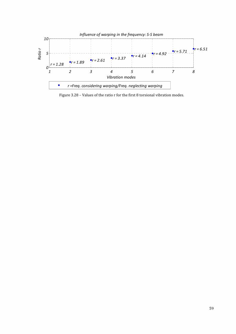
59

Figure 3.28 – Values of the ratio r for the first 8 torsional vibration modes.

1 2 3 4 5 6 7 80

5

10

Vibration modes

Ra

tio

r

Influence of warping in the frequency: S-S beam

r = 1.28 r = 1.89

r = 2.61 r = 3.37

r = 4.14 r = 4.92

r = 5.71 r = 6.51

r =Freq. considering warping/Freq. neglecting warping

61

4. FINITE ELEMENT APROXIMATION

The governing equations of thin-walled beams structural behavior are partial differential equations, being

the corresponding analytical solutions difficult to obtain for an arbitrary cross-section.

The finite element method (FEM) is a numerical method that allows to solve partial differential equations

approximately, and will be used in this chapter for solving the static and dynamic behavior of thin- walled beams.

The basic idea of FEM is to divide the beam into finite elements (finite element mesh) and obtain a numerical

solution by approximating the governing variables (e.g. displacements) in order to verify the governing

equations in a weak form.

For linear problems, the solution is obtained by solving a system of linear equations through a computer

code implementation, made by MATLAB in this analysis.

In FEM method the development of a finite element involves three principal steps (Fish & Belytschko, 2007):

1. The knowledge of the strong form, which consists of the governing equations for the model and the

boundary conditions formulation;

2. The weak form, which can be developed starting from the strong form through an integration by

parts;

3. The approximation functions, by which a displacement field will be modeled using shape functions

and nodal displacements vectors.

According to the Euler-Bernoulli theory a finite element has six degrees of freedom (DOF) for each end. In this

case, due to the deformability of thin-walled beam elements out of their own plane, another degree of freedom is

added representing the warping of the cross-section when it twists. This finite element with 7 DOF for each end

is developed and used to solve structural problems on continuous beams loaded generically.

Combining the approximation functions introduced for first in section 4.1 with the weak form of a general

differential equation it is possible to obtain the discrete finite element equations. In stress analysis these

equations solve the equilibrium of a general structure. The discretization will involve the calculus of element

matrices in order to describe the internal forces and the load acting upon the beam finite element. This is the

purpose of section 4.2, where the problem of uncoupled torsion is solved as a first approach, being developed

afterwards a beam element where coupled effect are considered.

In 4.3 an undamped vibration analysis is discretized by FEM method. In this case also inertial forces have to

be considered in order to verify the equations of motion for each degree of freedom. The inertial forces should be

described introducing an element mass matrix, which will be obtained for the uncoupled rotation of torsion and

then in the general case, where coupled effect must be taken into account.

4.1. Beam displacements discretization

The introduction of approximations and their definition is one of the principal parts of the FEM

development. The finite element can be convergent and the accuracy of a correctly developed FEM improves

with mesh refinement, i.e. as the element size describing the problem decreases the solution tends to the exact

solution. The two necessary conditions for convergence of the FEM are continuity and completeness (Fish &

Belytschko, 2007).

62

Under these assumptions two isoparametric beam elements are introduced in order to calculate the element

stiffness matrix, the element mass matrix and the element external force matrix. The key idea is to use the shape

functions to represent both the element geometry and the problem unknowns, which in this case are

displacements. Hence the name isoparametric element, often abbreviated to iso-P element.

4.1.1. Continuity

The choice of a function to describe a displacement field depends of the continuity required for the nodal

degrees of freedom of the element nodes. A function is called ±S function if its derivatives of order Ø for 0 ≤ Ø ≤ P exist and are continuous functions

on the entire domain. A ±; function is a linear function and is piecewise continuously differentiable, i.e. its fist

derivative is continuous except at selected points. So if a displacement is defined by a ±; function, the strain,

which corresponds to its derivative, is a ±úB function. This could be the case of the axial displacements, that

allow a linear approximation and do not require any continuity of their derivatives.

If the continuity of an approximation function is required also for its derivatives it should be a ±B function,

which has not kinks or jumps as discontinuities. This function will be used in the next section for the

approximation of bending and torsional displacements. The characteristics of ±úB, ±; and ±B functions are

illustrated, in terms of smoothness in the table 4.1, taken from (Fish & Belytschko, 2007).

Table 4.1 – Smoothness of functions (Fish & Belytschko, 2007).

Smoothness Kinks Jumps Comments ±úB Yes Yes Piecewise continuous

±; Yes No Piecewise continuously

differentiable

±B No No Continuously

differentiable

4.1.2. Approximation functions

Two-node linear element

Consider the simple one-dimensional element with two nodes as shown in figure 4.1. The approximation

functions for this kind of element must be ±; functions.

63

x,uξ=x / L

Ne

i

xxe

1

e

2

1 2

(x)Ne

1

(x)Ne

2

u

Le

1 2

u1 2

a) b)

Le

Figure 4.1 – Degrees of freedom and shape functions of the two node elements.

The global axis � passes through the bar axis and a non-dimensional coordinate � = �/� is introduced, being −1 ≤ � ≤ 1. This parent domain allows to consider the Gauss quadrature in order to define polynomial functions

that interpolate weight functions and trial solutions .

The relation between global and natural coordinates is written as follows

� = 12 (1 − �)�BÌ + 12 (1 + �)�>Ì = ûü ∙ ýü (4.1)

where the vector ûü = Q³BÌ ³>ÌR = B> Q(1 − �) (1 + �)R represents the element shape function and ýü = «�BÌ�>̬

represents the global coordinates.

The axial displacements of the bar, when one degree of freedom is considered for each end, are expressed in

the same form of the global coordinates by the shape functions as follows

�Ì = ûü ∙ þü (4.2)

being the vector of nodal displacements in axial direction defined as follows

þü = «�BÌ�>̬ (4.3)

It can be seen that the shape functions are linear in the element, as expected. This functions will be used for

the approximation of the axial displacement field.

Two-node Euler-Bernoulli element

The element shown in figure 4.2 is an Euler-Bernoulli beam element, which requires continuous nodal

displacement and rotation fields: this means that the trial solution and weight function approximations must be ±B functions,

64

x1 2

w1

w2

w'1

w'2

y

Le

Figure 4.2 - Two-node Euler-Bernoulli element.

The displacements and their first derivatives at nodes must be degrees of freedom of the element and the

class of functions generally used in this case are the Hermite polynomials, given by

�B = 1 4� (1 − �)>(2 + �) = 1 4� (2 − 3 � + ��) (4.4)

�> = �Ì 8� (1 − �)>(1 + �) = 1 4� (1 − � − �> + ��) (4.5)

�� = 1 4� (1 + �)>(2 − �) = 1 4� (2 + 3 � − ��) (4.6)

�½ = �Ì 8� (1 + �)>(� − 1) = 1 4� (−1 − � + �> + ��) (4.7)

where

� = 2��Ì − 1, −1 ≤ � ≤ 1 (4.8)

The shape functions are represented in (Fish & Belytschko, 2007). The displacement of the beam is defined

as follows

ÂÌ = �ü ∙ vü (4.9)

being the vector vü = QÂBÌ Â′BÌ Â>Ì Â′>ÌR the displacement vector and �ü = K�B �> ¡�> �� �½ ¡�> L the element

interpolation function matrix. Hence, Hermite polynomials will be used for describing bending and torsion with FEM discretization. Note

that in the case of torsion these functions do not represent the deformed shape of the beam element when it

twists, but they represent the values of the rotation and its first derivative.

4.2. The static formulation of the finite element

The differential equations obtained in chapter 3 describe the static problem in its strong form through the

kinematics of the beam, the constitutive relation and the equilibrium equation, imposing the correct boundary

conditions to the ends of the beam element. In section 4.2.1 a weak form will be developed starting from the

strong form of the torsion differential equation. The development of weak forms for bending and axial

differential equations are supposed to be already known.

The assembly of the seven degrees of freedom thin-walled beam element will be presented in section 4.2.2

with reference to two axes of reference as first approach: the elastic center and the shear center. Then the

element will be based on the elastic center only and coupling terms will appear in the element fundamental

matrices.

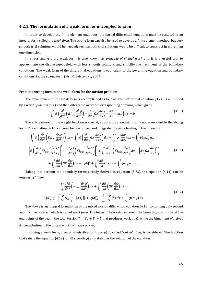
65

4.2.1. The formulation of a weak form for uncoupled torsion

In order to develop the finite element equations, the partial differential equations must be restated in an

integral form called the weak form. The strong form can also be used to develop a finite element method, but very

smooth trial solutions would be needed; such smooth trial solutions would be difficult to construct in more than

one dimension.

In stress analysis the weak form is also known as principle of virtual work and it is a useful tool to

approximate the displacement field with less smooth solutions and simplify the treatment of the boundary

conditions. The weak form of the differential equations is equivalent to the governing equation and boundary

conditions, i.e. the strong form (Fish & Belytschko, 2007).

From the strong form to the weak form for the torsion problem

The development of the weak form is accomplished as follows: the differential equation (3.74) is multiplied

by a weight function î(�) and then integrated over the corresponding domains, which gives:

2 î · 3>3�> ·W��� 3>�3�> ¸ − 33� D:= 3�3�E − 3�3� − ��¸ 3�¡; = 0

(4.10)

The arbitrariness of the weight function is crucial, as otherwise a weak form is not equivalent to the strong

form. The equation (4.10) can now be rearranged and integrated by parts leading to the following

2 î G 3>3�> ·W��� 3>�3�> ¸H 3�¡; − 2 î G 33� D:= 3�3�EH 3�¡

; − 2 î D3�3�E¡; 3� − 2 î����¡

; 3� =

wî G 33� ·W��� 3>�3�> ¸Hx;¡ − w3î3� G·W��� 3>�3�> ¸Hx;

¡ + 2 3>î3�> ·W��� 3>�3�> ¸¡; 3� − «î D:= 3�3�E¬;

¡

+ 2 3î3� D:= 3�3�E 3�¡; − Qî�R;¡ + 2 3î3� (�)¡

; 3� − 2 î��¡; 3� = 0

(4.11)

Taking into account the boundary terms already derived in equation (3.73), the equation (4.11) can be

written as follows

2 3>î3�> ·W��� 3>�3�> ¸¡; 3� + 2 3î3� D:= 3�3�E 3�¡

; =

Qî�Ã�R;¡ − «3î3� ���¬;¡ + Qî�ùR;¡ + {î�Ã|;¡ − 2 3î3� (�)¡

; 3� + 2 î����¡; 3�

(4.12)

The above is an integral formulation of the mixed torsion differential equation (4.10) containing only second

and first derivatives, which is called weak form. The terms in brackets represent the boundary conditions at the

end points of the beam: the total torsion �à = �Ã� + �ù + �à that produces work by î, while the bimoment ��� gives

its contribution to the virtual work by means of – ��@$ .

In solving a weak form, a set of admissible solutions �(�), called trial solutions, is considered. The function

that satisfy the equation (4.12) for all smooth î(�) is stated as the solution of the equation.

66

Minimum potential energy

The equation (4.12) can also be obtained by considering the principle of minimum potential energy. This

method has already been exposed in chapter 3. Considering eq.(3.72), the first variation of the potential energy

can be expressed in terms of the weight function by substituting Â(�) with the virtual displacements ²� and

considering the boundary terms, being written as follows:

²�(�) = 2 ·3>î3�> W��� 3>�3�> + 3î3� := 3�3� + � 3î3� − ��î¸ 3�¡; − ·Qî�ÃR;¡ − «3î3� ���¬;

¡¸ = 0 (4.13)

Notice that in eq.(4.10) the concentrated loads were defined by means of volume forces, while in (4.13) the

boundary terms are expressed directly.

The above, as already known, is the principle of virtual work, by which ²q = ²r. Thus, equation (4.13)

corresponds to (4.12) after rearranging the terms, as considered by the variational principles. The coincidence of

these two approaches will be useful in the next part of the analysis.

67

Discrete equations of the finite element

It is not required that the weight functions be approximated by the same interpolants that are used for the

trial solutions approximations; however, for most problem it is advantageous to use the same approximation for

these two kind of functions and the resulting method is called the Galerkin FEM. This method will be used and

the weight functions and trial solution are written as follows

�Ì(�) = �ü ∙ vü (4.14)

îÌ(�) = �ü ∙ �ü (4.15)

The angle of twist � is approximated in terms of Hermite’s functions above described for an Euler-Bernoulli

element. In fact, it has to be continuously differentiable and the dimensionless coordinate � is considered along

the beam axis. Thus, the twist angle expression can be written as follows:

�Ì(�) = �B�B + �> 3�B3� +���> +�½ 3�>3� (4.16)

where the following applies

3�Ü3� = 3�Ü3� �Ì2 (4.17)

being ¡> the jacobian of the beam element of length L taking into account the eq.(4.1). Substituting eq.(4.17) in the

first and second derivatives of �(�) gives

3��3� =2�� 3��3� ;32��3�2 = 4��2 32��3�2 (4.18)

Introducing the approximations of eq.(4.14) and eq.(4.15) and considering the jacobian into the eq.(4.12)

gives

�ü® 2 w 16�Ì ½ ·3>�ü3�> ¸è W��� ·3>�ü3�> ¸x vü �Ì2 3�BúB + 2 � 4�Ì > D3�ü3� Eè := D3�ü3� E B

úB vü �Ì2 3�− 2 �ü®B

úB �� �Ì2 3� + 2 2�Ì D3�ü3� EèBúB � �Ì2 3� − �ü®�ÃP|�� + 2�Ì D3�ü3� Eè ���P|��� = 0

(4.19)

In equation (4.19) Γ� represents the boundary nodes of the beam element and P is the normal vector: if � = −1 the P value is − 1, while P = 1 if � = +1.

óü represents the stiffness matrix of the element, which is given by

óü = 2 w 16�Ì ½ ·3>�ü3�> ¸è W��� ·3>�ü3�> ¸x vü �Ì2 3�BúB + 2 � 4�Ì> D3�ü3� Eè := D3�ü3� E B

úB vü �Ì2 3�= W����Ì� �12 6�Ì 4�Ì > −12 6�Ì−6�Ì 2�Ì > 12 −6�Ì 4�Ì>� + :=30�Ì �36 3�Ì 4�Ì > −36 3�Ì −3�Ì −�Ì> 36 −3�Ì 4�Ì>� (4.20)

The vector �ü is the element external force matrix, given by

68

�ü = 2 �ü®BúB �� �Ì2 3� − 2 2�Ì D3�ü3� EèB

úB � �Ì2 3� + �ü®�ÃP|�� − 2�Ì D3�ü3� Eè ���P|��

=}~~~~~~~��� �Ì2 − �

�� �Ì >12�� �Ì2 + �−�� �Ì>12 ���

������ + }~~

~� −�Ã(−1)−���(−1)�Ã(+1)���(+1) �����

(4.21)

After considering the assembling of óü and �ü, the expression for the entire structure is

�®�óv − �� = �®��� = � (4.22)

Where � is called residual. ó is the global stiffness matrix and f is the global external force matrix. Note that

this element can be used only if torsion is uncoupled from bending or extension of the beam element, as shown

in figure 4.3.

ϕ '(-1) 1

ϕ(1)ϕ '(1)

Le

ϕ(-1)

2

1

1

2

2

e

e

e

e

Figure 4.3 –Thin walled beam element subject to uncoupled torsion.

4.2.2. The thin-walled beam element considering an additional DOF of warping

When the shear center of a thin walled cross-section do not coincide with the elastic center, the torsion of a

generally loaded beam element is coupled with its flexural behavior.

For these kind of problems a finite element with 7 DOF at each end of the element is developed. This element

takes into account all the general displacements, in order to make an analysis of every thin-walled type of cross-

section.

The development of a coupled generic formulation of a thin-walled beam element is approached by the

variational principles.

As illustrated in the first part of this chapter, different types of approximation functions will be used for the

interpolation of the beam element generalized displacements. These approximation functions are summarized in

69

table 4.2. Note that ûü indicates linear interpolation functions for the element and ��ü indicates polynomial

Hermite’s interpolations.

Table 4.2 – Displacement field and approximation functions. Displacements Smoothness required Smoothness required Smoothness required Smoothness required for the approximationfor the approximationfor the approximationfor the approximation DDDDisplacement isplacement isplacement isplacement approximation functionsapproximation functionsapproximation functionsapproximation functions Nodal displacements vectorNodal displacements vectorNodal displacements vectorNodal displacements vector Axial

Piecewise

continuously

differentiable

%Ì(�) = ûü ∙ þü výü = «�BÌ�>̬

Bending

Continuously

differentiable ��Ì(�) = ��ü ∙ v�ü v�ü = QÂ�BÌ Â′�BÌ Â�>Ì Â′�>Ì R®

Continuously

differentiable ��Ì(�) = ��ü ∙ v�ü v�ü = QÂ�BÌ Â′�BÌ Â�>Ì Â′�>Ì R®

Torsion Continuously

differentiable �Ì(�) = ��ü ∙ v�ü v�ü = QÂ�BÌ Â′�BÌ Â�>Ì Â′�>Ì R®

In section 4.2.1 it is illustrated that two alternative methods can be used to formulate the FEM discretization,

the principle of virtual work or alternatively the minimum potential energy principle. This second approach is

used in the sequel to obtain the discrete equations in a matrix format. The final displacement approximation

could be considered as a vector as follows:

ü(�) = {%Ì(�) ��Ì(�) − ��<Ì(�) ��Ì(�) ��<Ì(�) �Ì(�) − �<Ì(�)|

= �ûü ��ü −

3��ü3� ��ü −3��ü3� ��ü −

3��ü3�

}~~~~~~� výüv�üv�üv�üv�üv�üv�ü���

�����

(4.23)

This approximation, which is composed by 7 DOF, describes the beam displacement field. The corresponding

element stiffness matrix is symmetric and constituted by 14 rows and 14 columns.

A first element stiffness matrix will be obtained considering two axes of reference for the displacements of

the cross-section, according to the static governing equations already derived in chapter 3. Then a second

stiffness matrix will be illustrated considering the element axes coincident with the elastic center axis. This

formulation will allow to define the displacement field, the stress distribution and the boundary conditions of the

element as referred to the same axis. This aspect could have several advantages in the analysis of straight

continuous beam elements with thin-walled section, i.e. complex frame structures and bridge models.

Axial effect

The first variation of the potential energy for a generic point � of the cross-section plan can be expressed as

follows when axial effect is considered

²�(²%, ²%<) = 2 W(6%<²%< − ����<<�²%< − ����<<�²%< − ����<<²%<)3�¡; − 2 �$²%¡

; 3� − Q³�²%R;¡ = 0 (4.24)

70

The equation (4.24) is equivalent to the weak form of the extension equilibrium with respect to a generic

point P when coupling is considered between all the generalized displacements. The discretization of the

equations according with (4.23) gives

• Element stiffness matrix

óü! = 2 � 4�Ì> D3ûü3� Eè W6 D3ûü3� E BúB výü �Ì2 3� − 12 2 � 8�Ì� D3ûü3� Eè W��� ·3>��ü3�> ¸ B

úB v�ü �Ì2 3�− 12 2 � 8�Ì� D3ûü3� Eè W��� ·3>��ü3�> ¸ B

úB v�ü �Ì2 3�− 12 2 � 8�Ì� D3ûü3� Eè W��� ·3>��ü3�> ¸ B

úB v�ü �Ì2 3� =

kz¡� K 1 −1−1 1 L výü − k¹ª">¡� K0 1 00 −1 0 −11 L v� − k¹ª#>¡� K0 1 00 −1 0 −11 L v� − k¹ª$>¡� K0 1 00 −1 0 −11 L v�

(4.25)

• External force vector

�ü! = 2 ûü®BúB �$ �Ì2 3� + ûü®³�P|�� = ��$ �Ì2�$ �Ì2 �+ «−³�B³�> ¬ (4.26)

where ³�B, ³�> refer to the axial forces at the end nodes of the beam element and are positive if directed as the

nodal displacements.

The internal forces that appear through the stiffness matrix are the effects of a general cross-section

deformation. As shown in figure 4.4 the application of the axial force in a generic point � generates four different

contributions: a uniform compression, bending in two directions and finally the warping of the section.

P4P P

=P

P

P

+

++

z

xy

P

P

P

P

P

PP

P

P

P

P

Eccentric axial force Uniform Compression Bending in (x,y) plan

Bending in (x,z) plan Warping of the cross-section

Figure 4.4 – Effects of the application of a general axial force on a thin walled beam (Cedolin, 1996).

71

Bending

As already done for the extension degree of freedom, the weak form is discretized starting from the first

variation of the potential energy for bending in two directions ²� �² �� , ²�<� , ²�<<� = 2 �−²�<<µW��µ%< + ²�<<µW��µ¶�<<¶ + ²�<<µW��µ��<< + �µ²�<µ − �µ²�µ ¡

; 3�− Q²�µ�õR;¡ + {²�<µ��µ|;¡

(4.27)

The repeated subscripts and � imply summation over = �, and � = �, .

Considering for simplicity only the �-direction and admitting the same approximations for test functions and

trial solutions, the discretized equation can be written as follows

• Element stiffness matrix

óü%� = − B> 5 « &¡�' �@Æ��ü@(Æ  è W��� �@ûü@(  ¬BúB výü ¡�> 3� + 5 « B)¡�* �@Æ��ü@(Æ  è W��� �@Æ��ü@(Æ  ¬ v�ü ¡�> 3�BúB +B> 5 « B)¡�* �@Æ��ü@(Æ  è W���� �@Æ��ü@(Æ  ¬ v�ü ¡�> 3�BúB + B> 5 « B)¡�* �@Æ��ü@(Æ  è W�� �� �@Æ��ü@(Æ  ¬ v�ü ¡�> 3�BúB =

k¹ª">¡� M 0 0 1 −1 0 0−1 1 N výü + kΪ"¡�' �12 6�Ì6�Ì 4�Ì> −12 6�Ì −6�Ì 2�Ì>−12 −6�Ì6�Ì 2�Ì> 12 −6�Ì−6�Ì 4�Ì>�v�ü +

B> kΪ"#¡�' � 12 6�Ì6�Ì 4�Ì> −12 6�Ì −6�Ì 2�Ì>−12 −6�Ì6�Ì 2�Ì> 12 −6�Ì−6�Ì 4�Ì>�v�ü + B> kΪ"$¡�' � 12 6�Ì6�Ì 4�Ì> −12 6�Ì −6�Ì 2�Ì>−12 −6�Ì6�Ì 2�Ì> 12 −6�Ì−6�Ì 4�Ì>�v�ü

(4.28)

• External force vector

�ü%� = 5 ��ü®BúB �� ¡�> 3� − 5 >¡� D@��ü®@( EBúB �� ¡�> 3� + ��ü®�Ã�P|�� − D@��ü®

@( E ���P|�� =}~~~~~��� ¡�> − ���� ¡�ÆB>�� ¡�> + ��−�� ¡�ÆB> ���

����

+}~~~~�

−�Ã�B−���B�Ã�>���> ������ (4.29)

For the flexural plane (�, ) the same matrices are obtained and will be written in the complete stiffness

matrix assembling.

Torsion

Uncoupled torsion has been already taken into account in its uncoupling form . When referred to the point P

the first variation of potential energy is written as follows:

²�(�) = 2 �−²�<<W���%< + ²�<<�����<<� + ²�<<�����<<� + ²�<<W�����<< + ²�<:=�< + �²�<¡; − ��²��3� − (Q²��ÃR;¡ − Q²�<���R;¡) (4.30)

Substituting the FEM discretization and applying the Galerkin FEM to the discretization yields the following:

72

óü� = − B> 5 « &¡�' �@Æ��ü@(Æ  è W��� �@ûü@(  ¬BúB výü ¡�> 3� + B> 5 « B)¡�* �@Æ��ü@(Æ  è W���� �@Æ��ü@(Æ  ¬ v�ü ¡�> 3�BúB +B> 5 « B)¡�* �@Æ��ü@(Æ  è W���� �@Æ��ü@(Æ  ¬ v�ü ¡�> 3�BúB + 5 « B)¡�* �@Æ��ü@(Æ  è W�� �� �@Æ��ü@(Æ  ¬ v�ü ¡�> 3�BúB =

− B> k¹ª$>¡� M 0 0 1 −1 0 0−1 1 N výü + B> kΪ$"¡�' � 12 6�Ì6�Ì 4�Ì> −12 6�Ì −6�Ì 2�Ì>−12 −6�Ì6�Ì 2�Ì> 12 −6�Ì−6�Ì 4�Ì>�v�ü +B> kΪ$#¡�' � 12 6�Ì6�Ì 4�Ì> −12 6�Ì −6�Ì 2�Ì>−12 −6�Ì6�Ì 2�Ì> 12 −6�Ì−6�Ì 4�Ì>�v�ü + kΪ$$¡�' � 12 6�Ì6�Ì 4�Ì> −12 6�Ì −6�Ì 2�Ì>−12 −6�Ì6�Ì 2�Ì> 12 −6�Ì−6�Ì 4�Ì>�v�ü +

ÔÕ�;¡� �36 3�Ì3�Ì 4�Ì> −36 3�Ì −3�Ì −�Ì>−36 −3�Ì3�Ì −�Ì> 36 −3�Ì−3�Ì 4�Ì>�v�ü

(4.31)

The external force matrix have already been written in eq.(4.21). Note that in the stiffness matrix the Saint

Venant contribution does not depends on the point P.

Assembly of the uncoupled matrix of the element

The results obtained in the discretization of the equilibrium equations can be assembled for all the

generalized displacements, allowing to write the element stiffness matrix.

It is convenient to write the elements of the vector of nodal displacements and the vector of associated nodal

forces in the following order

þü =

}~~~~~~~~~~~~~~~� �BÌÂ�BÌÂ′�BÌÂ�BÌÂ′�BÌÂ�BÌÂ′�BÌ�>ÌÂ�>ÌÂ′�>ÌÂ�>ÌÂ′�>ÌÂ�>ÌÂ′�>Ì ��

���������������

; �ü =

}~~~~~~~~~~~~~~~~~~~~~~~~~~~~~~� �$ �Ì2�� �Ì2 − ��

�� �Ì>12�� �Ì2 − ���� �Ì>12�� �Ì2 − �

�� �Ì>12�$ �Ì2�� �Ì2 + ��−�� �Ì>12�� �Ì2 + ��−�� �Ì>12�� �Ì2 + ��� �Ì>12 ��

������������������������������

+

}~~~~~~~~~~~~~~~~� −³�B−�Ã�B−���B−�Ã�B−���B−�ÃB−���B³�>�Ã�>���>�Ã�>���>�Ã>���> ��

����������������

(4.32)

73

In order to simplify the discrete equations, the displacement field will be referred to the elastic center for

axial effect and bending and to the shear center for the torsion as done for the equilibrium equations. This gives

for the stiffness matrix

óü =}~~~~~~~~� óü!+óü%�+óü%�+óü�+óü!õóü%�õóü%�õóü�õ ���

������� (4.33)

=

}~~~~~~~~~~~~~~~~~~~~~~~~~~~~~~~~~~~�W6�Ì 0 0 0 0 0 0 − W6�Ì 0 0 0 0 0 0

12 W���Ì�6W���Ì> 0 0 0 0 0 −12 W���Ì� 6W���Ì> 0 0 0 04 W���Ì 0 0 0 0 0 −6W���Ì> 2 W���Ì 0 0 0 0

12 W���Ì� 6W���Ì> 0 0 0 0 0 −12 W���Ì� 6W���Ì> 0 04 W���Ì 0 0 0 0 0 −6W���Ì> 2 W���Ì 0 0

12 W����Ì� + 3630 :=�Ì 6W����Ì> + 330 := 0 0 0 0 0 −12 W����Ì� − 3630 :=�Ì 6W����Ì> + 330 :=4 W����Ì + 430 :=�Ì 0 0 0 0 0 −6W����Ì> − 330 := 2 W����Ì − 130 :=�Ì

W6�Ì 0 0 0 0 0 012 W���Ì� −6W���Ì> 0 0 0 0

�������A 4 W���Ì 0 0 0 012 W���Ì� −6W���Ì> 0 0

4 W���Ì 0 012 W����Ì� + 3630 :=�Ì −6W����Ì> − 330 :=

4 W����Ì + 430 :=�Ì�������������������������������������

The 7 DOF element discretization have been completely defined and both nodal displacements and forces in

(4.32) and in (4.33) refer to two different axes. The axis considered for the beam generalized displacements in

order to uncoupling the effects of extension, bending and torsion are described in table 4.3,

Table 4.3 – Beam element displacements and corresponding axis of reference

Beam generalized displacements Axis of reference W��P-��P: ²% W��-�A A�P��: (�Å , Å) ï�P3�P�: ²�� , ²��< , ²�� , ²��< , ���-��P: ²�, ²�′ �ℎ��� A�P��: (�z, z)

74

The thin- walled beam element is represented by a generic example of a C-cross section in figure 4.5.

Elastic center axis (yC,zC)

Shear center axis (ya,za)

y

ξy

ξ z

η

ϕ

z

ϕ 'x

ξ 'z

ξ 'y2

22

2

2

2

2

ξ 'z1

ξ 'y1

ξz1

η1

ξy1

ϕ1

ϕ '1

2

2

11

Le

Figure 4.5 – Thin-walled C-beam element displacement referred to two axis.

Matrix of the element referred to the elastic center

The linear system defined by (4.32) and (4.33) describes the finite element approximation by means of two

axis. Taking into account this model the boundary conditions for the thin walled beam must be imposed on two

different axes according to the prescribed displacement of the general DOF.

The objective of the present analysis is to propose a discrete model in which only one axis is considered for

the beam element in order to obtain a stress analysis for continuous spans beams, i.e. a straight multi-spans

bridge deck. The axis chosen to describe the beam element is the elastic center: this means that kinematics,

strain and stresses, expressed by means of óü, �ü and þü, must refer to (�Å , Å) and a coupling between axial

effect, bending and torsion appears. Thus a sectorial coordinate �Šand the relative warping parameter �Š��

referred to the elastic center axis will be considered in the sequel. The stiffness matrix obtained is written as

follows:

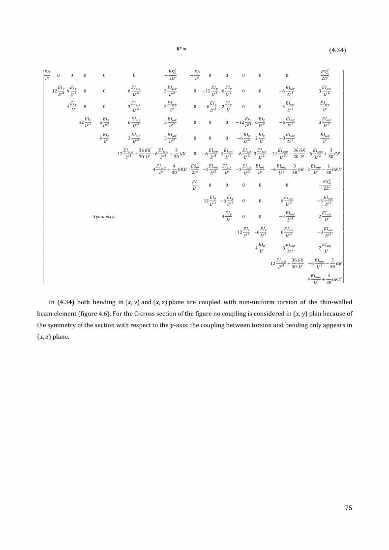
75

óü = (4.34)

}~~~~~~~~~~~~~~~~~~~~~~~~~~~~~~~~~~~~~~~~�W6�Ì 0 0 0 0 0 − W��Å2�Ì − W6�Ì 0 0 0 0 0 W��Å2�Ì

12 W���Ì� 6W���Ì> 0 0 6W����Ì� 3 W����Ì> 0 −12 W���Ì� 6W���Ì> 0 0 −6W����Ì� 3 W����Ì>4 W���Ì 0 0 3 W����Ì> 2 W����Ì 0 −6W���Ì> 2 W���Ì 0 0 −3 W����Ì> W����Ì

12 W���Ì� 6W���Ì> 6W����Ì� 3 W����Ì> 0 0 0 −12 W���Ì� 6W���Ì> −6W����Ì� 3 W����Ì>4 W���Ì 3 W����Ì> 3 W����Ì> 0 0 0 −6W���Ì> 2 W���Ì −3 W����Ì> W����Ì

12 W����Ì� + 3630 :=�Ì 6W����Ì> + 330 := 0 −6W����Ì� 3 W����Ì> −6W����Ì� 3 W����Ì> −12 W����Ì� − 3630 :=�Ì 6W����Ì> + 330 :=4 W����Ì + 430 :=�Ì W��Å2�Ì −3 W����Ì> W����Ì −3 W����Ì> W����Ì −6W����Ì> − 330 := 2 W����Ì − 130 :=�Ì

W6�Ì 0 0 0 0 0 − W��Å2�Ì12 W���Ì� −6W���Ì> 0 0 6W����Ì� −3 W����Ì>

�������A 4 W���Ì 0 0 −3 W����Ì> 2 W����Ì12 W���Ì� −6W���Ì> 6W����Ì� −3 W����Ì>

4 W���Ì −3 W����Ì> 2 W����Ì12 W����Ì� + 3630 :=�Ì −6W����Ì> − 330 :=

4 W����Ì + 430 :=�Ì������������������������������������������

In (4.34) both bending in (�, �) and (�, ) plane are coupled with non-uniform torsion of the thin-walled

beam element (figure 4.6). For the C-cross section of the figure no coupling is considered in (�, �) plan because of

the symmetry of the section with respect to the �-axis: the coupling between torsion and bending only appears in

(�, ) plane.

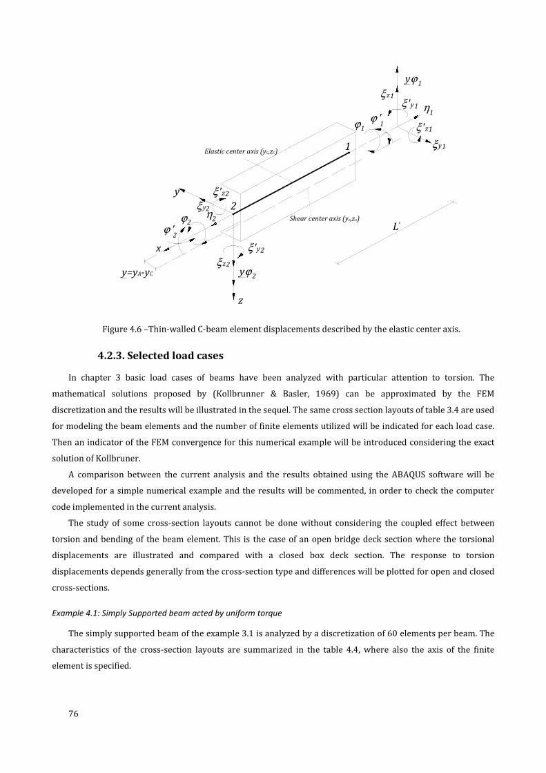
76

Elastic center axis (yC,zC)

Shear center axis (ya,za)

y

ξy

ξ z

ηϕ

z

ϕ 'x

ξ 'z

ξ 'y2

2

2

2

2

2

2

ξ 'z1

ξ 'y1

ξ z1

η1

ξy1

ϕ1

ϕ '1

2

1

y=yA-yC yϕ2

yϕ1

Le

Figure 4.6 –Thin-walled C-beam element displacements described by the elastic center axis.

4.2.3. Selected load cases

In chapter 3 basic load cases of beams have been analyzed with particular attention to torsion. The

mathematical solutions proposed by (Kollbrunner & Basler, 1969) can be approximated by the FEM

discretization and the results will be illustrated in the sequel. The same cross section layouts of table 3.4 are used

for modeling the beam elements and the number of finite elements utilized will be indicated for each load case.

Then an indicator of the FEM convergence for this numerical example will be introduced considering the exact

solution of Kollbruner.

A comparison between the current analysis and the results obtained using the ABAQUS software will be

developed for a simple numerical example and the results will be commented, in order to check the computer

code implemented in the current analysis.

The study of some cross-section layouts cannot be done without considering the coupled effect between

torsion and bending of the beam element. This is the case of an open bridge deck section where the torsional

displacements are illustrated and compared with a closed box deck section. The response to torsion

displacements depends generally from the cross-section type and differences will be plotted for open and closed

cross-sections.

Example 4.1: Simply Supported beam acted by uniform torque

The simply supported beam of the example 3.1 is analyzed by a discretization of 60 elements per beam. The

characteristics of the cross-section layouts are summarized in the table 4.4, where also the axis of the finite

element is specified.

77

Table 4.4 – Cross-section layout characteristics.

Cross-section Characteristics Axis of reference for the FEM

analysis

Closed hollow section

b = 100 mm; h = 360 mm;

t = tw = tf = 14 mm; �ÉÊËËÊÇ +ÌC. = 19.89

Elastic center (coincident with the

shear center)

Channel cross Section

b = 100 mm; h = 360mm;

t = tw = tf = 14mm; �Å +ÌC. = 1.5

Shear center

I cross Section

b = bf1 = bf2 = 170mm ; h=360mm;

tf = 12.7mm, tw = 8mm; �Î +ÌC. = 1.19

Elastic center (coincident with the

shear center)

The coordinate system considered is represented in figure 4.7.

L

ξ= / L

L/2

Figure 4.7 – Non-dimensional coordinate system.

The boundary conditions are described in table 4.5.

Table 4.5 – Boundary conditions of the beam.

Coordinate Static boundary prescribed Kinematic boundary prescribed � = −0.5 ��(−0.5) = 0 �(−0.5) = 0 � = +0.5 ��(+0.5) = 0 �(+0.5) = 0

The results in terms of displacements and internal forces are obtained solving the linear system composed

by eq.(4.20) and eq.(4.21) and are represented in the figure 4.8,figure 4.9,figure 4.10 and figure 4.11 where the

normalized �, �<, ��, � distributions along the beam axis are depicted (Dotted line: FEM model; Continuous line:

analytical solution).

Figure 4.8 – � value of a S-S beam acted by uniform torque (FEM solution).

-0.5 -0.4 -0.3 -0.2 -0.1 0 0.1 0.2 0.3 0.4 0.5

-0.1

0

0.1

0.2

ξ

φ*

GK

/mL2

Twist angle normalized

C I Hollow

78

Figure 4.9 – �′ value of a S-S beam acted by uniform torque (FEM solution).

Figure 4.10 - �� of a S-S beam acted by uniform torque (FEM solution).

Figure 4.11 – Torsion � of a S-S beam acted by uniform torque (FEM solution). Example 4.2: Concentrated load on a simply supported beam

In this example, the exact solution of the load case 3.2 will be approximated by the FEM for obtain the twist

rotation of the beam, its first derivative, the warping moment and the relatives contributions of torsion. The

same coordinate system of figure 4.7 for the same cross-section layouts is used and the boundary conditions for

the problem are written in table 4.5. figure 4.12, figure 4.13, figure 4.14 and figure 4.15 show the results

obtained(Dotted line: FEM model; Continuous line: analytical solution).

-0.5 -0.4 -0.3 -0.2 -0.1 0 0.1 0.2 0.3 0.4 0.5

-0.5

0

0.5

ξ

φ'*

GK

/mL

First derivative of twist angle normalized

C I Hollow

-0.5 -0.4 -0.3 -0.2 -0.1 0 0.1 0.2 0.3 0.4 0.5

0

0.05

0.1

0.15

0.2

ξ

Mw

/mL2

Mw normalized

C I Hollow

-0.5 -0.4 -0.3 -0.2 -0.1 0 0.1 0.2 0.3 0.4 0.5

-0.5

0

0.5

ξ

T/m

L

Torsion T: relative influence of Ts

C I Hollow Total torsion

79

Figure 4.12 – � value of a S-S beam acted by concentrated torque (FEM solution).

Figure 4.13 – �′ value of a S-S beam acted by concentrated torque (FEM solution).

Figure 4.14- �� of a S-S beam acted by concentrated torque (FEM solution).

-0.5 -0.4 -0.3 -0.2 -0.1 0 0.1 0.2 0.3 0.4 0.5

0

0.1

0.2

0.3

0.4

ξ

φ*

GK

/mL2

Twist angle normalized

C I Hollow

-0.5 -0.4 -0.3 -0.2 -0.1 0 0.1 0.2 0.3 0.4 0.5

-0.5

0

0.5

ξ

φ'*

GK

/mL

First derivative of twist angle normalized

C I Hollow

-0.5 -0.4 -0.3 -0.2 -0.1 0 0.1 0.2 0.3 0.4 0.5

0

0.1

0.2

0.3

0.4

ξ

Mw

/mL2

Mw normalized

C I Hollow

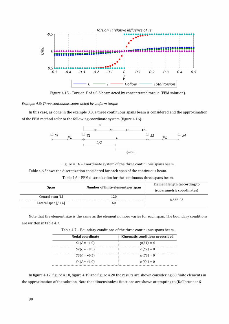
80

Figure 4.15 - Torsion � of a S-S beam acted by concentrated torque (FEM solution).

Example 4.3: Three continuous spans acted by uniform torque

In this case, as done in the example 3.3, a three continuous spans beam is considered and the approximation

of the FEM method refer to the following coordinate system (figure 4.16).

Lj*L j*LS1 S2 S3 S4

L/2

ξ= / L

Figure 4.16 – Coordinate system of the three continuous spans beam.

Table 4.6 Shows the discretization considered for each span of the continuous beam.

Table 4.6 – FEM discretization for the continuous three spans beam.

Span Number of finite element per span Element length (according to

isoparametric coordinates)

Central span [�] 120 8.33E-03

Lateral span [, ∗ �] 60

Note that the element size is the same as the element number varies for each span. The boundary conditions

are written in table 4.7.

Table 4.7 – Boundary conditions of the three continuous spans beam.

Nodal coordinate Kinematic conditions prescribed �1(� = −1.0) �(�1) = 0 �2(� = −0.5) �(�2) = 0 �3(� = +0.5) �(�3) = 0 �4(� = +1.0) �(�4) = 0

In figure 4.17, figure 4.18, figure 4.19 and figure 4.20 the results are shown considering 60 finite elements in

the approximation of the solution. Note that dimensionless functions are shown attempting to (Kollbrunner &

-0.5 -0.4 -0.3 -0.2 -0.1 0 0.1 0.2 0.3 0.4 0.5

-0.5

0

0.5

ξ

T/m

L

Torsion T: relative influence of Ts

C I Hollow Total torsion

81

Basler, 1969) in order to be independent from the geometry of the problem(Dotted line: FEM model; Continuous

line: analytical solution).

Figure 4.17 - � value of a T-C-S5 beam acted by uniform torque (FEM solution).

Figure 4.18 - �′ value of a T-C-S beam acted by uniform torque (FEM solution).

Figure 4.19 - �� of a T-C-S beam acted by uniform torque (FEM solution).

5 Three continuous spans.

-1 -0.8 -0.6 -0.4 -0.2 0 0.2 0.4 0.6 0.8 1

0

0.05

0.1

ξ

φ*

GK

/mL2

φ normalized C,I and Hollow sections

C I Hollow

-1 -0.8 -0.6 -0.4 -0.2 0 0.2 0.4 0.6 0.8 1

-0.5

0

0.5

ξ

φ'*

GK

/mL

φ' normalized C,I and Hollow sections

C I Hollow

-1 -0.8 -0.6 -0.4 -0.2 0 0.2 0.4 0.6 0.8 1

-0.1

-0.05

0

0.05

0.1

ξ

Mw

/mL2

Mw normalized C,I and Hollow sections

C I Hollow

82

Figure 4.20 – Tosion � of a T-C-S beam acted by uniform torque (FEM solution).

Example 4.4: Convergence of the FEM discretization

With the FEM approximation the results obtained for a load case must be compared with the analytical

results. For this reason it is useful to include a parameter allowing to estimate the error in the finite element

solution. The rate of convergence of this approximated solution can be observed increasing the number of

elements, according to the refinement type h.

The example 4.3 of a continuous three-spans beam is considered as an example, where 240 elements are

used for the analysis of the entire beam. The table 4.8 shows the error variation of ��/(��>) at the internal

support S2 (see figure 4.16) taking into account a different element length for each approximation, which

correspond to consider every FEM mesh with a different number of elements. The total number of elements used

in modeling the entire beam is shown in the table, while the number of elements used for the discretization of

the central span is half of the total number of elements.

Table 4.8 – Decrease of the relative error of ��/(��>) for different finite element meshes.

Element size 12.5E-02

(8 Elem.)

8.33E-02

(12 Elem.)

6.25E-02

(16 Elem.)

5E-02

(20 Elem.)

1.25-02

(80 Elem.)

8.33E-03

(120 Elem.)

4.17E-03

(240 Elem.) Exact value

��/(��>)(�2) 0.0286 0.0386 0.0437 0.0468 0.0564 0.0575 0.0586 0.0597

Relative Error 0.52% 0.35% 0.27% 0.22% 0.06% 0.04% 0.02%

The values of the normalized warping moment can be represented as a function of the number of elements

used for the discretization of the central span. This function is represented in figure 4.21 where a semi-

logarithmic scale is used for the mid-span number of elements.

-1 -0.8 -0.6 -0.4 -0.2 0 0.2 0.4 0.6 0.8 1

-0.5

0

0.5

ξ

Ts/

mL

Torsion T: relative influence of Ts

C I Hollow T

83

Figure 4.21 – Convergence of the �� value as function of the mesh refinement.

The analytical value of the normalized warping moment is -0.597 and the analysis performed in the example

4.3 leads to a good approximation of the solution. Note that the warping moment according to the eq.(3.95) is

mathematically described by hyperbolic functions and in the finite element model Hermite polynomials were

adopted.

Example 4.5: Comparative study between ABAQUS model and current analysis

The software ABAQUS has in its library (Hibbit, 2007) a 7 DOF beam element to perform the analysis of open

thin-walled beam cross-sections. This type of element can be used for the study of thin-walled beams, whenever

warping cannot be neglected. The characteristics for the element B31OS (Hibbit, 2007) are sketched in Figure

4.22.

Figure 4.22 – ABAQUS element B310S and integration points for I-beam section.

In this case the FEM approximation will be checked for the three load cases preformed above and I-section.

The characteristics of the section and the ABAQUS element are illustrated in table 4.9. The table 4.10 shows the

results obtained for each load case and estimates the relative error between the two analysis methods, using for

the ABAQUS simulation the same number of elements. The normal tension V$ is calculated at the extreme point

of the I-section flange, i.e. the point number 1 in the I-section presented by figure 4.22.

100

101

102

103

-0.06

-0.05

-0.04

-0.03

Number of finite elements of the midspan

Wa

rpin

g m

om

en

t o

n t

he

su

pp

ort

Mw = -0.0286

Mw = -0.0386

Mw = -0.0437

Mw = -0.0468

Mw = -0.0564 Mw = -0.0575

Mw = -0.0586

Values FEM aproximation Exact

Number of finite elements of the central span

Table 4.9 – Characteristics of the beam Elements loaded.

STATIC CHARACTERISTICS

BOUNDARY CONDITION LOADING SECTION ÷øø Q-.R ELEMENT

(ABAQUS) Nº of elements

Nº integration

points for the

cross-section

L

S-S (L=2m)

Uniform torque

distributed

I-Section 3.14E-07 B31OS

60

13 Lj*L j*L

m

S1 S2 S3 S4

T-C-S (L=2m;j=0.5)

Uniform torque

distributed acting

upon the middle

span

240

L

S-S (L=2m)

Concentrated

moment at

midspan

60

Table 4.10 – Comparison of results between current model and ABAQUS element.

Load case

ROTATION �(max)

ERROR

BICURVATURE �''(max)

ERROR

BIMOMENT /ø(max) [N.m]

ERROR

0ýý(max) [kPa]

ERROR ABAQUS Current analysis ABAQUS Current analysis ABAQUS Current analysis ABAQUS Current analysis

S-S

(uniform load) 2.80E-03 2.80E-03 0.14% 6.59E-03 6.60E-03 0.12% 434.10 436.00 0.45% 2.04E+07 2.05E+07 0.44%

T-C-S

(load on the

central span)

1.24E-03 1.20E-03 -3.42% 3.56E-03 3.50E-03 -1.55% 234.10 233.70 -0.17% 1.10E+07 1.10E+07 -0.17%

SS

(Concent. load) 2.25E-03 2.20E-03 -2.38% 6.67E-03 6.80E-03 2.00% 439.00 448.60 2.20% 2.07E+07 2.11E+07 2.19%

84

85

It can be verified from the table 4.10 that the relative error between the present analysis and the ABAQUS

beam element does not exceed 3.5% in terms of the angle of twist � value and that the approximation of normal

stress depends directly from the warping moment value.

This check could be considered as a FEM model indicator for its numerical implementation and the accuracy

performed leads to a good approximation of the ABAQUS results.

Example 4.6: Coupled behavior of typical bridge cross-sections

A continuous three-spans beam is analyzed as a structural model of a highway bridge deck. The longitudinal

model of the numerical example is represented in figure 4.23.

3 0 4 0 3 0

x

Figure 4.23 - Longitudinal model of a bridge numerical example.

This practical example is analyzed taking into account two cross-section layouts: the closed box section

represented by figure 4.24, which is typically used for these structural solutions, and a double-T cross-section,

which is represented in figure 4.25.

2,6

13,3

0,5

0,3

5

0,1

55,6

z

y

0,5

Figure 4.24 – Box-section of the bridge deck.

z

y

3,2

0,8

0,5

0,1

5

0,3

5

13,3

Figure 4.25 – Double-T section of the bridge deck.

The loading on a bridge section, according to EN 1991-2, can be considered as an eccentric line load applied

in the -direction. This vertical type of load generates bending and torsion of the deck, as represented in figure

4.26.

86

2m 3m

Tandem Load Lane Load

Qik

qik

Figure 4.26 – Lane model for general types of vertical loads.

The cross-sections represented are compared as two possible structural solutions for the bridge design. For

this reason have been chosen considering approximately the same moment of inertia �� in the flexural plan (�, )

obtained in relation to the elastic center. The bending characteristics of the two cross-section are given in the

table 4.11.

Table 4.11 – Flexural characteristics of the bridge deck cross-sections.

Cross-section layout Height 1 Q-R Slenderness 2 of

the mid-span Moment of inertia ÷�Q-3R

Box 2.6 10.8 8.10

Double-T 3.2 8.75 8.99

The slenderness of the bridge section is defined by the ratio 4 = ¡5, being � = 0.7 ∗ �; and �; the length of the

central span.

The geometry of the referred cross-sections are defined by the respective mid-line, being the correspondent

dimensions given in table 4.12.

87

Table 4.12 – Section properties of the bridge cross-sections.

Box Section Double-T Section

Bb b

h tw

tfC

z

y

ab1

E

tf1

Bb b

h tw tw

tfC

z

y

ïQ�R 7.30 6.65 �Q�R 3.00 3.33 ÇQ�R 0.50 0.80 ÈQ�R 0.35 0.35 ÈBQ�R 0.30 - 23° - ℎQ�R 2.28 3.03

The torsional behavior of the two different cross-sections, as already presented, is described by the

calculation of the non-dimensional parameter �, which involves both material and section properties and also

the geometry of the structure through the mid-span length �Ü . These quantities are listed in table 4.13.

Table 4.13 – Cross-section properties and torsion parameters.

Box section Double-T

Section W Q:��R 33.00 : Q:��R 13.75 =Q�½R 17.14 1.17 ��� Q�½R 54.47 110.14 �ÜQ�R 40.00 κ 14.9 2.66

The elastic modulus W and the shear modulus : corresponds to a concrete class C30/37 considered for the

bridge deck. All the coordinate distributions of the cross-section, which were used to define the properties

summarized in table 4.13 are presented in the annex A.

By applying the constitutive law to Saint Venant torsion (3.78), the ratio between the torsion parameters of

the two sections can be obtained:

=8Ê$ +ÌC9ÜÊS=ÊíÌS +ÌC9ÜÊS = �′9Ê$ +ÌC9ÜÊS�′ÊíÌS +ÌC9ÜÊS = 14.65 (4.35)

The = magnitude greatly exceeds that of the open sections, being the := value the first source of torsional

stiffness for all the compact solid and hollow sections.

88

In the sequel it will be considered the loading represented in figure 4.27 and figure 4.28 adopting �� = 1 and � = 1.

C

z

yC

z

y

e e

PZ PZ

Figure 4.27 – Loading in the cross-section plane.

1kN

4030 30

1 kN/m

x

z

+

S1 S2 S3 S4

Figure 4.28 –Loading in the longitudinal direction.

As a first approach only the double-T section will be analyzed. This section is asymmetric with respect to �-

axis and an additional �-displacement due to torsion will appear when twist is considered in the elastic center, as

illustrated in figure 4.29. This effect is the same shown in figure 4.6 when the finite element have been

assembled considering the elastic center axis for reference.

C

z

y

A

ϕ z

ϕz

Figure 4.29 – Coupling effect between torsion and transversal displacement.

The displacement field due to the loading represented in figure 4.28 is obtained by using the FEM model,

being the coupling effect illustrated in figure 4.29 considered by using the element stiffness matrix (4.34).

The boundary prescriptions for FEM model are listed in table 4.14.

89

Table 4.14 – Boundary displacement fixed at nodes.

Nodal coordinate Boundary conditions prescribed �1(� = 0) ��(�1) = ��(�1) = �(�1) = 0 �2(� = 30 �) ��(�2) = ��(�2) = �(�2) = 0 �3(� = 70 �) ��(�3) = ��(�3) = �(�3) = 0 �4(� = 100 �) ��(�4) = ��(�4) = �(�4) = 0

The results are presented in figure 4.30 for the transversal displacements and the twist.

Cuy

C

uz

Cϕ

Figure 4.30 – Displacements and rotation of the bridge model with double-T section (FEM model).

As already mentioned, there are no bending displacements in (�, �) plane but the twist around the shear

center generates a transversal displacement �� of the elastic center axis, as shown in figure 4.30.

In terms of internal forces, the shear diagram and bending moments in (�, ) plane are represented in figure

4.31. The torsion moment and the bimoment distribution along the beam axis are represented in figure 4.32.

0 10 20 30 40 50 60 70 80 90 100

-1

0

1

x 10-6

Displacement of the2 d.o.f

0 10 20 30 40 50 60 70 80 90 100

-5

0

5

x 10-5

Displacement of the4 d.o.f

0 10 20 30 40 50 60 70 80 90 100

-2

0

2

x 10-6

Displacement of the6 d.o.f

[m]

[m]

[rad]

x[m]

x[m]

x[m]

90

z

xV z

z+dVz

z

x

zz+dMz

Figure 4.31 – Shear force �� and bending moment �� along the elastic center axis.

z

M t+dMtxM t

z

M ω+dMωxM ω

Figure 4.32 – Torsion moment �9 and warping moment �� along the elastic center axis.

A comparison between the double-T section analyzed and the box section, considering the warping effect,

can be described by showing the different torsional behavior. The �-rotation of the box section compared

between box-section and double-T section is shown in

figure 4.33, while is represented in

figure 4.34 the Saint Venant torsion �¹ = �′:= along the bridge axis for the same two examples of deck

section.

0 10 20 30 40 50 60 70 80 90 100

-2

0

2

x 104

0 10 20 30 40 50 60 70 80 90 100

-2

0

2

x 105

Internal forces of the5 d.o.f

0 10 20 30 40 50 60 70 80 90 100

-2

0

2

x 104

0 10 20 30 40 50 60 70 80 90 100

-1

0

1

x 105

[N]

x[m]

x[m]

[N.m]

x[m]

x[m]

[N.m]

[N.m2]

91

Figure 4.33 - Twist values along the beam axis for the double-T section and for the Box section.

Figure 4.34 – Saint Venant torsion contribution for the double-T section and for the Box section.

It can be observed that as expectable the Saint Venant contribution to the total torsion of the bridge is almost

the totality.

Notice that when coupled effect is considered, the value of the warping parameter used is referred to the

elastic center and is ���Š. The coupling is expressed by the terms in the stiffness matrix involving ���Š. Details of

calculus about these quantities are also illustrated in the Annex 1.

Example 4.7: Torsion behavior and accuracy of the solutions

The problem of mixed torsion have been examined by three load cases and an approximation have been

proposed for the analysis of thin-walled beams. The effect of warping for more cross-section layouts can be

evaluated in order to present general results and classify typical section behaviors with respect to torsion.

A dimensionless presentation of the results can be done if the warping moments ��(�) are compared with

the warping moment ��(� = 0) when only warping torsion is considered. Results between 1 and 0 of the ratio ��(�)/��(� = 0) indicate the torsion response of beam-elements loaded by uniform or concentrated torque.

The graph demonstrate that within large regions of small and large �-values one torsional component may

be neglected as opposed to the other without appreciable error. The results obtained by the FEM for the loading

and beams presented in examples 4.1,4.2 and 4.3 are represented in figure 4.35 by a semi-logarithmic scale.

0 10 20 30 40 50 60 70 80 90 100

-5

0

5

10

x 10-7

Double-T deck Box deck

0 10 20 30 40 50 60 70 80 90 100

-2

0

2

x 104

Ts

Double-T deck Box deck

�[rad]

�¹[N.m]

�[m]

�[m]

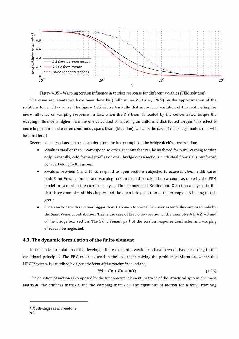
92

Figure 4.35 – Warping torsion influence in torsion response for different �-values (FEM solution).

The same representation have been done by (Kollbrunner & Basler, 1969) by the approximation of the

solutions for small �-values. The figure 4.35 shows basically that more local variation of bicurvature implies

more influence on warping response. In fact, when the S-S beam is loaded by the concentrated torque the

warping influence is higher than the one calculated considering an uniformly distributed torque. This effect is

more important for the three continuous spans beam (blue line), which is the case of the bridge models that will

be considered.

Several considerations can be concluded from the last example on the bridge deck’s cross-section:

• �-values smaller than 1 correspond to cross-sections that can be analyzed for pure warping torsion

only. Generally, cold formed profiles or open bridge cross-sections, with steel floor slabs reinforced

by ribs, belong to this group.

• �-values between 1 and 10 correspond to open sections subjected to mixed torsion. In this cases

both Saint Venant torsion and warping torsion should be taken into account as done by the FEM

model presented in the current analysis. The commercial I-Section and C-Section analyzed in the

first three examples of this chapter and the open bridge section of the example 4.6 belong to this

group.

• Cross-sections with �-values bigger than 10 have a torsional behavior essentially composed only by

the Saint Venant contribution. This is the case of the hollow section of the examples 4.1, 4.2, 4.3 and

of the bridge box section. The Saint Venant part of the torsion response dominates and warping

effect can be neglected.

4.3. The dynamic formulation of the finite element

In the static formulation of the developed finite element a weak form have been derived according to the

variational principles. The FEM model is used in the sequel for solving the problem of vibration, where the

MDOF6 system is described by a generic form of the algebraic equations:

/:ä + ;:­ + ó: = t(J) (4.36)

The equation of motion is composed by the fundamental element matrices of the structural system: the mass

matrix /, the stiffness matrix ó and the damping matrix ; . The equations of motion for a freely vibrating

6 Multi-degrees of freedom.

10-1

100

101

102

0

0.2

0.4

0.6

0.8

1

κ

Mw

(κ)/

Mw

(pu

re w

arp

ing

)

Warping increasing ratio

S-S Concentrated torque

S-S Uniform torque

Three continuous spans

93

undamped system can be obtained by omitting the damping matrix and the applied load from (4.36), yielding the

following equation:

/:ä + ó: = � (4.37)

The element stiffness matrix for the FEM model has already been obtained.

An element mass matrix will be deduced in section 4.3.1 for the uncoupled problem of torsion by taking into

account the kinetic energy of the beam element. The coupling between generalized displacements for

asymmetric sections can be taken into account, being a general element mass matrix obtained through

variational principles in section 4.3.2 for a 7 DOF beam element. This matrix will refer, as already done for the

stiffness matrix, to the elastic centre axis of the beam element.

When all the matrices in eq. (4.37) are known and assembled for the system analyzed, the discrete equation

can be solved by a frequency analysis: frequency equations of the system are polynomial equations that allow to

obtain for each DOF a mode of vibration. The mode shapes and the mode frequency are the solution of an

eigenvalues equation that will be solved by FEM model in 4.3.3.

In the analysis of thin walled beam section examples of uncoupled vibration will be shown in the selected

cases 4.3.4 and also coupled examples of free vibration in thin-walled element analysis will be compared.

4.3.1. The formulation of a weak form for the uncoupled torsion

The variational principles have been applied for the static case in order to obtain a system of discrete and

linear equations. The equivalent in dynamics is the application of the Hamilton’s principle. The differential

equations for uncoupled torsion is defined by (3.125) and the terms in this equation refer to the shear center 6.

If the shear centre S coincides with the elastic center C the bending of the beam is uncoupled from its torsion.

This consideration gives the following equation

−¯��� 0>0�> ·0>�0> ¸ + ¯���z + ��z� 0>�0> + 0>0�> ·W��� 0>�0�> ¸ − 00� D:= 3�3�E − 3�3� − �� = 0 (4.38)

Notice that in the equation (3.125), which was studied by (Gere, 1954) and presented in chapter 3, is

neglected the inertial contribution of warping displacement, while in the present work all the parcels will be

considered. This equation can be multiplied by the virtual rotation î, called weight function, and then integrated

on the domain of the element (as already done in static): this gives the weak form. Alternatively, the principle of

Hamilton can be used and, considering the boundary terms out of the integral, gives

2 2 ¯�����<ä î< + �íz�ä î�3�3 +¡;

9Æ9æ 2 2 (�<<W���î<< + �<:=î< − ��î + �î′)3�3¡

;9Æ

9æ− 2 ·Qî�ÃR;¡ − «3î3� ���¬;

¡¸ 39Æ9æ = 0

(4.39)

where �íz = ���z + ��z� is the polar moment of inertia. Applying the Galerkin FEM to the functions in eq.(4.39) a

discrete linear equation can be expressed: the first term defines the mass element matrix while all the other

terms of (4.39) have already been presented. The approximation functions are the Hermite polynomials and the

separation of variables made by (4.14) and (4.15) allow to refer the time derivatives of the functions �(�, ) and î(�, ) to the nodal displacement vectors∙ vü and ∙ �ü. In fact, notice that if the time-depending terms are

omitted the equation (4.39) corresponds to the (4.13).

The substitution of the approximation functions in (4.39) gives

94

�ü® 2 � 4�Ì> D3�ü3� Eè ¯��� D3�ü3� E vüä �Ì2 3�BúB + 2 {�üè¯�s6�ü|vüä �Ì2 3�B

úB+ 2 w 16�̽ ·3>�ü3�> ¸è W��� ·3>�ü3�> ¸x vü �Ì2 3�B

úB + 2 � 4�Ì> D3�ü3� Eè := D3�ü3� E BúB vü �Ì2 3�

− 2 �ü®BúB �� �Ì2 3� + 2 2�Ì D3�ü3� EèB

úB � �Ì2 3� − �ü®�ÃP|�� + 2�Ì D3�ü3� Eè ���P|��� = 0

(4.40)

The linear equation expressed by (4.40) refers to the simple case in which shear center and elastic center

points coincide, which occurs for the I-Beam of Figure 4.3. Note that the coincidence between these two points

implies that �íz = �í = �� + ��.

The first and second terms constitute the contribution of the inertia forces and their integration over the

parent domain yields the consistent mass matrix that is written as follows:

/ü = 2 � 4�Ì> D3�ü3� Eè ¯��� D3�ü3� E vüä �Ì2 3�BúB + 2 {�üè¯�s6�ü|vüä �Ì2 3�B

úB= ¯���30�Ì �36 3�Ì 4�Ì> −36 3�Ì −3�Ì −�Ì> 36 −3�Ì 4�Ì >�+ ¯�s�Ì420 �156 22�Ì 4�Ì> 54 −13�Ì 13�Ì −3�Ì> 156 −22�Ì 4�Ì> �

(4.41)

After considering the assembling of /ü, óü and �ü over the entire number of beam elements the expression

of the discrete equation is given by:

�®�/vä + óv − �� = �®��� = � (4.42)

where � is the residual.

4.3.2. The element mass matrix considering an additional DOF of warping

The discretization of the equation of motion for a generic problem, where coupled inertial effects are

considered, requires the knowledge of a consistent mass matrix for the thin-walled beam element. The

displacement field is approximated by the function listed in table 4.2, which corresponds to a set of 7 generalized

displacements at each end of the derived finite element. The stiffness matrix óü and the internal forces vector

�ühave already been defined and the objective of this part is to derive the mathematical formulation of the

element mass matrix /ü. The approach will be similar to the one used in the formulation of the stiffness matrix.

A first element mass matrix will be obtained considering two axes of reference for the displacements of the

cross-section, according to the equations of motion already derived in chapter 3. Then, a second mass matrix will

be derived considering the element axis coincident with the elastic center axis.

Axial effect

The Hamilton principle for a generic point P of the cross-section plane is applied considering the generalized

displacement %. The kinetic energy per unit length of the axial effect is given by

�(%­) = 12 ¯(6%­> − ���%­�­�< − ���%­�­�< − ���%­�­ <) (4.43)

The equation (4.43) can be substituted in eq.(3.101) in order to obtain, after suitable rearrangements, the

following

95

2 129Æ9æ ¯ 2 �26%ä − �����<ä − �����<ä − ����<ä   ²%3�3¡

;+ 2 2 W(6%<²%< − ����<<�²%< − ����<<�²%< − ����<<²%<)3�3¡

;9Æ

9æ− 2 2 �$²%¡

; 3�39Æ9æ − 2 Q³�²%R;¡9Æ

9æ = 0

(4.44)

The first term represents the contribution of mass and after substituting the displacement approximation

functions, it allows to obtain the mass matrix as follows

/ü! = 2 {ûüè¯6ûü|BúB výä ü �Ì2 3� − 12 2 � 2�Ì ûüè¯��� ·3��ü3� ¸ B

úB v�ä ü �Ì2 3�− 12 2 � 2�Ì ûüè¯�� � ·3��ü3� ¸ B

úB v�ä ü �Ì2 3� − 12 2 � 2�Ì ûüè¯��� ·3��ü3� ¸ BúB v�ä ü �Ì2 3�

= ¯6�Ì6 K2 11 2L výä ü − ¯���24 K−6 �Ì 6−6 −�Ì 6 −�Ì�Ì L v�ä ü − ¯���24 K−6 �Ì 6−6 −�Ì 6 −�Ì�Ì L v�ä ü− ¯���24 K−6 �Ì 6−6 −�Ì 6 −�Ì�Ì L v�ä ü

(4.45)

Also the mass contribution of the axial displacements involves coupling between axial effect, bending and

torsion. The first term is the consistent mass matrix of the finite element considering axial displacement, while

the other terms are the off-diagonal terms of the mass matrix. Note that the sum of all the terms in the first

matrix is ¯6�Ì , which is the total mass of the beam, while the sum of the other masses is 0 given of the fact that

the displacement field considered correspond to the flexural and torsional degrees of freedom.

Bending

As already done for the beam’s extension, the variational principle is imposed and only the displacement ��

is considered for the moment. The corresponding expression of the kinetic energy is given by

� ��­� , �­�<  = 12 ¯(−����­�<%­ + ����­�<> + ����­�<�­�< + �����­�<�­ < + 6��­ > − ��­ ����­ ) (4.46)

Substituting the kinetic energy per unit length (4.46) in (3.101) and rearranging the terms gives

2 129Æ9æ ¯ 2 �−���%ä + 2�����<ä + ������<ä + �����<ä   ²�<�3�3¡

; + 2 129Æ9æ ¯ 2 �26��ä − ����ä �²��3�3¡

;+ 2 12 2 (−²�<<�W���%< + 2²�<<�W�����<<� + ²�<<�W�� ��<<� + ²�<<�W�� ���<<)3�3¡

;9Æ

9æ− 2 2 (−��²�<� + ��²��)¡

; 3�39Æ9æ − 2 D{²���Ã�|;¡ − K²�<����L;

¡E9Æ9Æ = 0

(4.47)

Considering the same approximations for test functions and trial solutions (Galerkin approach) the

discretized equation in �- direction of the mass matrix gives

96

/ü%� = − B> 5 « >¡� �@��ü@(  è ¯���ûü¬BúB výä ü ¡�> 3� + 5 « ½¡�Æ �@��ü@(  è ¯��� �@��ü@(  ¬BúB v�ä ü ¡�> 3� +5 {��üè¯6��ü|BúB v�ä ü ¡�> 3� + B> 5 « ½¡�Æ �@��ü@(  è ¯���� �@��ü@(  ¬BúB v�ä ü ¡�> 3� +B> 5 « ½¡�Æ �@��ü@(  è ¯���� �@��ü@(  ¬BúB v�ä ü ¡�> 3� − B> 5 {��üè¯�����ü|BúB v�ä ü ¡�> 3� =− <¹ª">½ K−6 �Ì 6−6 −�Ì 6 −�Ì�Ì Lè výä ü + <Ϊ"�;¡� �

36 3�Ì 4�Ì> −36 3�Ì −3�Ì −�Ì> 36 −3�Ì 4�Ì>� v�ä ü +<z¡�½>; �

156 22�Ì 4�Ì > 54 −13�Ì 13�Ì −3�Ì> 156 −22�Ì 4�Ì > � v�ä ü + B> <Ϊ"#�;¡� �36 3�Ì 4�Ì> −36 3�Ì −3�Ì −�Ì> 36 −3�Ì 4�Ì >� v�ä ü +

B> <Ϊ"$�;¡� �36 3�Ì 4�Ì> −36 3�Ì −3�Ì −�Ì > 36 −3�Ì 4�Ì >� v�ä ü − B> <¹#ª½>; �

156 22�Ì 4�Ì > 54 −13�Ì 13�Ì −3�Ì> 156 −22�Ì 4�Ì > � v�ä ü

(4.48)

For the flexural plane (�, ) a similar form is obtained and will be written in the final form of the mass matrix.

Torsion

Torsion has already been taken into account in its uncoupling form. When referred to the generic point P the

kinetic energy of torsion per unit length is given by

�(�­ , �­ <) = 12 ¯(−����­ <%­ + �����­ <�­�< + �����­ <�­�< + �����­ <> − ��­ ����­ + ��­ ����­ + ���� + �����­ >) (4.49)

The application of the Hamilton principle implies that the following applies:

2 12 ¯ 2 D�−���%ä + ������ä < + �����ä�< + 2�����ä <  ²�< + �−��ä ��� + ��ä ��� + 2���� + �����ä �²�E¡;

9Æ9æ 3�3

+ 2 2 �−²�<<W���%< + ²�<<W�����<<� + ²�<<W�����<<� + ²�<<W�����<<¡;

9Æ9æ

+ ²�<:=�< + �²�< − ��²�� 3�3 − 2 (Q²��ÃR;¡ − Q²�<���R;¡)39Æ9æ = 0

(4.50)

Considering the approximations for the displacement field, in the context of the FEM formulation,

substituted in the first integral of (4.50) gives for the mass matrix

97

/ü� = − 12 2 w 2�Ì ·3��ü3� ¸è ¯��� ûüxBúB výä ü �Ì2 3� + 12 2 w 4�Ì> ·3��ü3� ¸è ¯���� ·3��ü3� ¸xB

úB v�ä ü �Ì2 3�− 12 2 K��üè¯����üLB

úB v�ä ü �Ì2 3� + 12 2 w 4�Ì> ·3��ü3� ¸è ¯���� ·3��ü3� ¸xBúB v�ä ü �Ì2 3�

+ 12 2 K��üè¯�����üLBúB v�ä ü �Ì2 3� + 2 w 4�Ì> ·3��ü3� ¸è ¯���� ·3��ü3� ¸xB

úB v�ä ü �Ì2 3�+ 2 K��üè¯ ��� + ��� ��üLB

úB v�ä ü �Ì2 3�= − ¯���24 K−6 �Ì 6−6 −�Ì 6 −�Ì�Ì Lè výä ü + 12 ¯�� ��30�Ì �36 3�Ì 4�Ì> −36 3�Ì −3�Ì −�Ì> 36 −3�Ì 4�Ì>� v�ä ü

− 12 ¯����Ì420 �156 22�Ì 4�Ì> 54 −13�Ì 13�Ì −3�Ì> 156 −22�Ì 4�Ì> � v�ä ü + 12 ¯����30�Ì �36 3�Ì 4�Ì> −36 3�Ì −3�Ì −�Ì> 36 −3�Ì 4�Ì>� v�ä ü

+ 12 ¯����Ì420 �156 22�Ì 4�Ì> 54 −13�Ì 13�Ì −3�Ì> 156 −22�Ì 4�Ì> � v�ä ü + ¯����30�Ì �36 3�Ì 4�Ì> −36 3�Ì −3�Ì −�Ì> 36 −3�Ì 4�Ì>� v�ä ü

+ ¯ ��� + ��� 420 �156 22�Ì 4�Ì> 54 −13�Ì 13�Ì −3�Ì> 156 −22�Ì 4�Ì> � v�ä ü

(4.51)

Assembly of the consistent mass matrix

In order to simplify the discrete equations, the displacement field will be referred to the elastic center for

axial effect and bending and to the shear center for the torsion as done for the equilibrium equations. The same

assumption has been used in the first formulation of the stiffness element matrix and thus the mass matrix can

be assembled in a systematic way that gives

/ü =}~~~~~~~~�/ü!+/ü%�+/ü%�+/ü�+/ü!õ/ü%�õ/ü%�õ/ü�õ ���

�������

= (4.52)

}~~~~~~~~~~~~~~~~~~~~~~~~~~~~~~~~~~~~~~~~~~~~~~�<z¡�� 0 0 0 0 0 0 <z¡�) 0 0 0 0 0 0

�)�; <Î"¡� + B=)½>; ¯6�Ì ��; ¯�� + >>½>; ¯6�Ì> 0 0 0 0 0 − �)�; <Î"¡� + =½½>; ¯6�Ì ��; ¯�� − B�½>; ¯6�Ì> 0 0 0 0½�; ¯���Ì + ½½>; ¯6�Ì� 0 0 0 0 0 − ��; ¯�� + B�½>; ¯6�Ì>− B�; ¯���Ì − �½>; ¯6�Ì� 0 0 0 0

�)�; <Î#¡� + B=)½>; ¯6�Ì ��; ¯�� + >>½>; ¯6�Ì> 0 0 0 0 0 − �)�; <Î#¡� + =½½>; ¯6�Ì ��; ¯�� − B�½>; ¯6�Ì> 0 0½�; ¯���Ì + ½½>; ¯6�Ì� 0 0 0 0 0 − ��; ¯�� + B�½>; ¯6�Ì>− B�; ¯���Ì − �½>; ¯6�Ì� 0 0

�)�; <Î$$¡� + B=)½>; ¯�íz�Ì ��; ¯��� + >>½>; ¯�íz�Ì> 0 0 0 0 0 − �)�; <Î$$¡� + =½½>; ¯�íz�Ì ��; ¯��� − B�½>; ¯�íz�Ì>

½�; ¯����Ì + ½½>; ¯�íz�Ì� 0 0 0 0 0 − ��; ¯��� + B�½>; ¯�íz�Ì>− B�; ¯����Ì − �½>; ¯�íz�Ì�

<z¡�� 0 0 0 0 0 0�)�; <Î"¡� + B=)½>; ¯6�Ì − ��; ¯�� − >>½>; ¯6�Ì> 0 0 0 0

�������A ½�; ¯���Ì + ½½>; ¯6�Ì� 0 0 0 0�)�; <Î#¡� + B=)½>; ¯6�Ì − ��; ¯�� − >>½>; ¯6�Ì> 0 0

½�; ¯���Ì + ½½>; ¯6�Ì� 0 0�)�; <Î$$¡� + B=)½>; ¯�íz�Ì − ��; ¯��� − >>½>; ¯�íz�Ì>

½�; ¯����Ì + ½½>; ¯�íz�Ì� ������������������������������������������������

98

99

The beam mass described by the matrix is located in two different points of the cross-section. Hence, the

inertia forces are uncoupled each others (Friberg, 1985). The element is defined as shown in figure 4.36.

Elastic center axis (yC,zC)

Shear center axis (ya,za)

y

ξy

ξz

η

ϕ

z

ϕ 'x

ξ 'z

ξ 'y2

22

2

2

2

2

ξ 'z1

ξ 'y1

ξz1

η1

ξy1

ϕ1

ϕ '1

2

2

11

. .

.

.

.

.

.

..

.

.

.

.

.

Le

Figure 4.36 –Thin-walled C-beam element and uncoupled kinematic field.

In the current analysis, the finite element will be derived referring the all governing equations to the elastic

center, which as a consequence will produce a coupling between axial effect, bending and torsion. The mass

matrix considering (�Å , Å) as reference for the kinetic of the thin-walled beam is

/ü = (4.53)

}~~~~~~~~~~~~~~~~~~~~~~~~~~~~~~~~~~~~~~~~~~~~~~�¯6�Ì3 0 0 0 0 624 ¯�Å � − 124 ¯�Å ��Ì ¯6�Ì6 0 0 0 0 − 624 ¯�Å � 124 ¯�Å ��Ì

3630 ¯���Ì + 156420 ¯6�Ì 330 ¯�� + 22420 ¯6�Ì> 0 0 1830 ¯�Å���Ì 360 ¯�Å�� 0 − 3630 ¯���Ì + 54420 ¯6�Ì 330 ¯�� − 13420 ¯6�Ì> 0 0 − 1830 ¯�Å���Ì 360 ¯�Å��430 ¯���Ì + 4420 ¯6�Ì� 0 0 360 ¯�Å�� 460 ¯�Å���Ì 0 − 330 ¯�� + 13420 ¯6�Ì>− 130 ¯���Ì − 3420 ¯6�Ì� 0 0 − 360 ¯�Å�� − 160 ¯�Å ���Ì

3630 ¯���Ì + 156420 ¯6�Ì 330 ¯�� + 22420 ¯6�Ì> 1830 ¯�Å ���Ì 360 ¯�Å�� 0 0 0 − 3630 ¯���Ì + 54420 ¯6�Ì 330 ¯�� − 13420 ¯6�Ì> − 1830 ¯�Å���Ì 360 ¯�Å��430 ¯���Ì + 4420 ¯6�Ì� 360 ¯�Å �� 460 ¯�Å ���Ì 0 0 0 − 330 ¯�� + 13420 ¯6�Ì>− 130 ¯���Ì − 3420 ¯6�Ì� − 360 ¯�Å�� − 160 ¯�Å���Ì

3630 ¯����Ì + 156420 ¯�íz�Ì 330 ¯��� + 22420 ¯�íz�Ì> 624 ¯�Å � − 1830 ¯�Å���Ì 360 ¯�Å�� − 1830 ¯�Å���Ì 360 ¯�Å�� − 3630 ¯����Ì + 54420 ¯�íz�Ì 330 ¯��� − 13420 ¯�íz�Ì>

430 ¯����Ì + 4420 ¯�íz�Ì� 124 ¯�Å ��Ì − 360 ¯�Å�� − 160 ¯�Å���Ì − 360 ¯�Å�� − 160 ¯�Å���Ì − 330 ¯��� + 13420 ¯�íz�Ì>− 130 ¯����Ì − 3420 ¯�íz�Ì�

¯6�Ì3 0 0 0 0 − 624 ¯�Å � − 124 ¯�Å��Ì

3630 ¯���Ì + 156420 ¯6�Ì − 330 ¯�� − 22420 ¯6�Ì> 0 0 1830 ¯�Å���Ì − 360 ¯�Å��

�������A 430 ¯���Ì + 4420 ¯6�Ì� 0 0 − 360 ¯�Å�� 460 ¯�Å���Ì

3630 ¯���Ì + 156420 ¯6�Ì − 330 ¯�� − 22420 ¯6�Ì> 3630 ¯�Å���Ì − 330 ¯�Å��430 ¯���Ì + 4420 ¯6�Ì� − 330 ¯�Å�� 430 ¯�Å ���Ì

3630 ¯����Ì + 156420 ¯�íz�Ì − 330 ¯��� − 22420 ¯�íz�Ì>

430 ¯����Ì + 4420 ¯�íz�Ì� ������������������������������������������������

10

0

101

The element defined by (4.52) is exemplified in figure 4.37 by a C-beam.

Elastic center axis (yC,zC)

Shear center axis (ya,za)

y

ξy

ξz

ηϕ

z

ϕ 'x

ξ 'z

ξ 'y2

2

2

2

2

2

2

ξ 'z1

ξ 'y1

ξ z1

η1

ξ y1

ϕ1

ϕ '1

2

1

y=yA-yC yϕ 2

yϕ1

Le

..

.

.

..

.

.

.

.

.

.

.

.

.

.

Figure 4.37 - Thin-walled C-beam element and coupled kinematic field.

4.3.3. The undamped free-vibration

In the discussion presented in chapter 3 the dynamical behavior of a beam element has been investigated by

a set of SDOF systems represented by single differential equations.

However, in general, the dynamic response of a structure cannot be described adequately by a SDOF model.

In fact, the structure dynamics behavior can be described only in terms of more than one degree of freedom. In

the development of the equations of motion for the MDOF beam finite element, which is object of this analysis, all

the discretized equation will refer to the structural-property matrices of motion of a general system.

The motion of a beam element have been defined by general displacements of a set of discrete points on the

beam and the corresponding equation of motion, treated in chapter 3 for selected points of the cross-section

plane. These equations can be written for each axis reference by expressing the dynamic equilibrium of the

effective forces associated with each degree of freedom. When the force vectors are presented in matrix form, the

MDOF equivalent of (3.96) is written as follows:

�÷ + �> + �? = �(J) (4.54)

where the subscripts indicate inertia, damping and elastic forces, while �(J) is the externally applied load for

each degree of freedom.

In the next part, the undamped free-vibration motion will be considered. This means that �>=0 and, in

general, for civil structures the damping influence is relatively low.

Mode shapes and mode frequencies

The problem of vibration analysis for a MDOF system consists of obtaining the conditions under which

(4.37) will allow motions to occur. By analogy with the behavior of SDOF systems, it can be assumed that the

102

free-vibration motion is simple harmonic, which may be expressed for a MDOF system as (Clough & Penzien,

1982)

:(J) = :@ sin(s + A) (4.55)

where :@ represents the shape of the system, s is the radian frequency and A is a phase angle.

When the second time derivative of (4.55) is taken, the accelerations in free vibration are given by

:ä = −s>:@ sin(s + A) = −s>: (4.56)

Substituting (4.55) and (4.53) into (4.37) gives

−s>/:@ sin(s + A) + ó:@ sin(s + A) = � (4.57)

in which � is a zero vector. The equation (4.57) may be written as follows:

Qó − s>/R:@ = � (4.58)

A nontrivial solution for this set of simultaneous equations is possible only when

‖ó − s>/‖ = � (4.59)

The equation (4.59) is called frequency equation of the system and is an equation of ³th degree in the

frequency parameter s> for a system having ³ degrees of freedom. The ³ roots of this equation represent the

frequencies of the ³ modes of vibration, which are possible in the system. The modes are sorted by ascending

values of frequency; thus the first mode is the one having the lowest frequency and so on. The vector made up of

the entire set of modal frequencies, arranged in sequence, will be called frequency vector t and is written as

follows

t = MsBs>⋮sDN (4.60)

When the frequencies of vibration are obtained by (4.59) a new matrix can be defined by subtracting sS>/

from the stiffness matrix, which yields

öO = ó − sS>/ (4.61)

Since it depends on the frequency, it is different for each mode. The equation (4.58) is satisfied identically

and the amplitude of the vibrations is indeterminate, but the shape of the vibrating system can be obtained by

solving for all the displacements in terms of any coordinate.

With this process the shape of the N vibration modes can be found and the square matrix made up of the ³

mode shapes will be represented by

� = �îBBî>B⋮îDB…⋱…

îBDî>D⋮îDD� (4.62)

This means that the vibration analysis of a structural system is a form of eigenvalue problem of matrix-

algebra theory: the modal frequencies are the eigenvalues and the mode shapes are the eigenvectors. Note that

this matrix constists of ³ independent modal vectors, thus it is nonsingular and can be inverted.

The vibrating shapes have special properties that are useful in structural-dynamics analysis: the

orthogonality relationships. For a detailed exposition of these properties and for their demonstration see

(Clough & Penzien, 1982). The orthogonality conditions can be expressed as follows

�-® /�O = 0 � ≠ P (4.63)

�-® ó�O = 0 � ≠ P (4.64)

103

Where �, P are two different modes of a structural system. These conditions show that the vibrating shapes

are orthogonal with respect to the stiffness matrix as well as to the mass.

Normal coordinates

The mode shapes constitute ³ independent displacement patterns, the amplitude of which may serve as

generalized coordinates to express any type of displacement. Thus, a much more useful representation of the

displacements can be provided by the free-vibration mode shapes.

Any displacement vector : for the structure can be developed by superposing suitable amplitudes of the

modes of vibration. For any modal component :@O, the displacements are given by the mode-shape vector �O

multiplied by the modal amplitude GS; thus

:@O = �OGS (4.65)

Then the total displacement is obtained as a sum of the modal components as follows:

: = H�OGSD

STB = �I (4.66)

The mode-shape matrix serves to transform the generalized coordinates I into the cartesian coordinates :.

In order to evaluate any arbitrary normal coordinate GS , the equation (4.66) can be multiplied by the product

of the transpose of the corresponding modal vector and the mass matrix �O®/. This gives

�O®/: = �O®/�I (4.67)

The right-hand side of this equation can be expanded in a series where all the terms vanish except that

corresponding to �O because of the orthogonality property (4.63). This consideration leads to

�O®/: = �O®/�OGS (4.68)

which allows to obtain the modal amplitudes as follows:

GS = �O®/:�O®/�O (4.69)

GS represents the participation of the P-vibration mode in the global response of the structure. The modal

participation factor allows to establish the vibration influence of each degree of freedom in a particular mode. 4.3.4. Examples

The analysis presented deals with the free-torsional vibrations of thin-walled beams with open cross-section

in which the shear center can or not coincide with the elastic center. An I-Beam will be analyzed by the FEM

model and torsional vibrations will be studied in their uncoupled form for different boundary prescriptions. The

vibration modes will be derived directly with the corresponding modal frequency.

The results obtained will be compared with the case in which warping of the section is neglected for

different boundary conditions and for different vibration modes. Note that the case of a cross-section which does

not warp is a limiting case of the general problem.

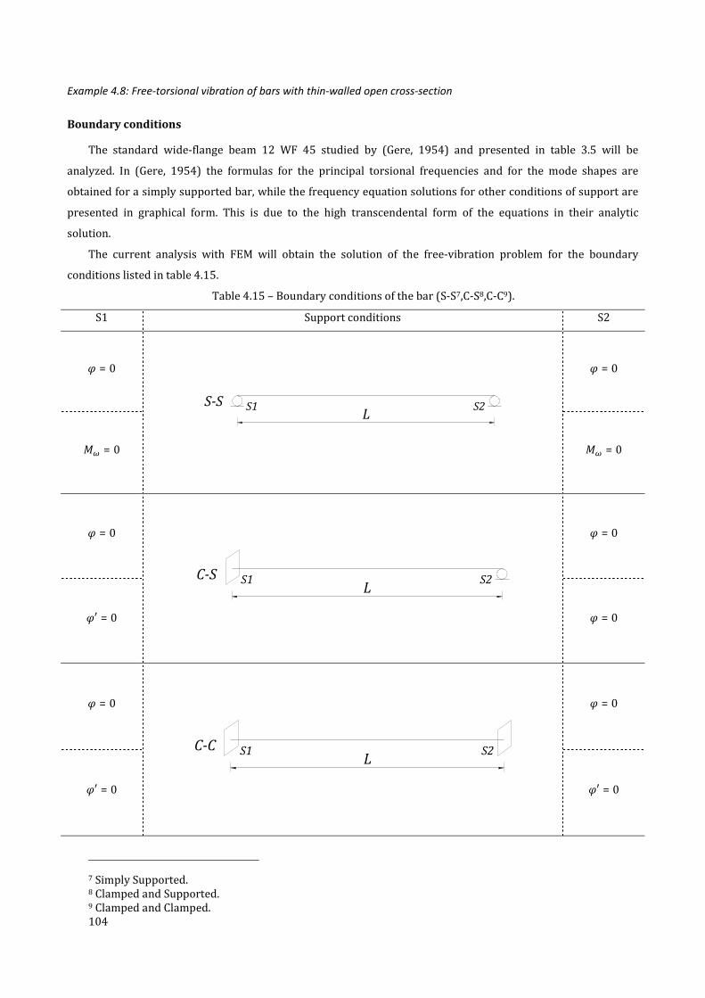
104

Example 4.8: Free-torsional vibration of bars with thin-walled open cross-section

Boundary conditions

The standard wide-flange beam 12 WF 45 studied by (Gere, 1954) and presented in table 3.5 will be

analyzed. In (Gere, 1954) the formulas for the principal torsional frequencies and for the mode shapes are

obtained for a simply supported bar, while the frequency equation solutions for other conditions of support are

presented in graphical form. This is due to the high transcendental form of the equations in their analytic

solution.

The current analysis with FEM will obtain the solution of the free-vibration problem for the boundary

conditions listed in table 4.15.

Table 4.15 – Boundary conditions of the bar (S-S7,C-S8,C-C9).

S1 Support conditions S2

� = 0

LS-S S1 S2

� = 0

�� = 0 �� = 0

� = 0

LC-S S1 S2

� = 0

�′ = 0 � = 0

� = 0

LC-C S1 S2

� = 0

�′ = 0 �′ = 0

7 Simply Supported. 8 Clamped and Supported. 9 Clamped and Clamped.

105

The theoretical analysis made in the example 3.4 shows the influence of warping in increasing the beam

frequency. This effect is expectable since warping increases the stiffness of the bar against twisting and can be

verified separating the different contributions of the element stiffness matrix (4.20) as follows

óü = óö÷øøü + óòóü (4.70)

The element mass matrix (4.41) for the uncoupled problem also can be seen as summation of two

contributions, thus

/ü = /÷øøü + /÷tü (4.71)

The mass considered by (Gere, 1954) is the contribution due to the polar inertia �í , being the inertial effect

related to the warping through ��� neglected by (Gere, 1954). Thus, the element mass matrix considered for

reproducing the values of ratio � given in eq.(3.129) consists of only the contribution /÷tü . The denominator of � is obtained considering óü = óòóü .

The ratio � between frequencies will be calculated for the first 8 vibration modes and is shown in figure 4.38,

figure 4.39 and figure 4.40 for a discretization of 60 elements per beam. Notice that the results represented by

figure 4.38 are the same of those obtained in figure 3.28 with the analytical expression. The length of the beam is

assumed to be the same of the one considered by Gere (Length � = 6�(20 Á) with � = 4).

Figure 4.38 - Ratio r for 8 vibration modes in a S-S beam. Solution obtained by the presented model.

Figure 4.39 - Ratio r for 8 vibration modes in a C-S beam. Solution obtained by the presented model.

1 2 3 4 5 6 7 80

5

10

Vibration modes

Ra

tio

r

Influence of warping in the frequency: S-S beam

r = 1.28 r = 1.89

r = 2.61 r = 3.36

r = 4.14 r = 4.92

r = 5.71 r = 6.5

r =Freq. considering warping/Freq. neglecting warping

1 2 3 4 5 6 7 80

5

10

Vibration modes

Ra

tio

r

Influence of warping in the frequency: C-S beam

r = 1.65 r = 2.28

r = 3 r = 3.76

r = 4.53 r = 5.32

r = 6.1 r = 6.89

r =Freq. considering warping/Freq. neglecting warping

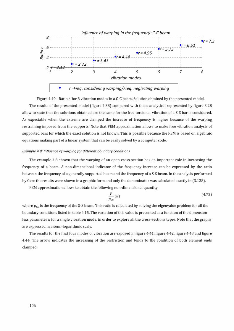
106

Figure 4.40 - Ratio r for 8 vibration modes in a C-C beam. Solution obtained by the presented model.

The results of the presented model (figure 4.38) compared with those analytical represented by figure 3.28

allow to state that the solutions obtained are the same for the free torsional-vibration of a S-S bar is considered.

As expectable when the extreme are clamped the increase of frequency is higher because of the warping

restraining imposed from the supports. Note that FEM approximation allows to make free vibration analysis of

supported bars for which the exact solution is not known. This is possible because the FEM is based on algebraic

equations making part of a linear system that can be easily solved by a computer code.

Example 4.9: Influence of warping for different boundary conditions

The example 4.8 shown that the warping of an open cross-section has an important role in increasing the

frequency of a beam. A non-dimensional indicator of the frequency increase can be expressed by the ratio

between the frequency of a generally supported beam and the frequency of a S-S beam. In the analysis performed

by Gere the results were shown in a graphic form and only the denominator was calculated exactly in (3.128).

FEM approximation allows to obtain the following non-dimensional quantity

ss¹¹ (�) (4.72)

where s¹¹ is the frequency of the S-S beam. This ratio is calculated by solving the eigenvalue problem for all the

boundary conditions listed in table 4.15. The variation of this value is presented as a function of the dimension-

less parameter � for a single vibration mode, in order to explore all the cross-sections types. Note that the graphs

are expressed in a semi-logarithmic scale.

The results for the first four modes of vibration are exposed in figure 4.41, figure 4.42, figure 4.43 and figure

4.44. The arrow indicates the increasing of the restriction and tends to the condition of both element ends

clamped.

1 2 3 4 5 6 7 82

4

6

8

Vibration modes

Ra

tio

r

Influence of warping in the frequency: C-C beam

r = 2.12 r = 2.72

r = 3.43 r = 4.18

r = 4.95 r = 5.73

r = 6.51 r = 7.3

r =Freq. considering warping/Freq. neglecting warping

107

κ

Figure 4.41 - Influence of boundary conditions on the 1st mode frequency.

κ

Figure 4.42 - Influence of boundary conditions on the 2nd mode frequency.

κ

Figure 4.43- Influence of boundary conditions on the 3rd mode frequency.

10-1

100

101

102

1

1.5

2

2.5

p/p

(SS)

S-S

C-S

C-C

10-1

100

101

102

1

1.1

1.2

1.3

1.4

1.5

1.6

1.7

κ

p/p

(SS)

S-S

C-S

C-C

10-1

100

101

102

1

1.1

1.2

1.3

1.4

κ

p/p

(SS)

Influence in the mode3 of boundary conditions and warping in beam frequencies

S-S

C-S

C-C

108

κ

Figure 4.44 - Influence of boundary conditions on the 4th mode frequency.

Notice that, as expectable, for lower �-values the increase of the frequency is more evident and by

restraining warping in both ends, the ratio reaches values of 230% for the first vibration mode.

When the torsion response of the section tends to pure Saint Venant torsion (� > 15) the value of s/s¹¹(�)

is low and the warping influence on increasing the frequency is not so high. These conclusions prove that the

results obtained are more relevant for open thin-walled cross-sections, being the boundary conditions of

warping restrained an important factor to be accounted, which greatly increases the vibration frequency of these

beam-like elements. The increasing of the modal frequency for higher vibration modes is smaller, even for the

cases of pure warping torsion, because these modes have higher frequency values the effect of restraining

warping affects less the stiffness as the modal frequency increases.

Example 4.10: Modal analysis of a Simply Supported beam

The equation of motion expressed by the FEM model neglecting the damping and the applied loads allows to

obtain the vibration modes and the frequency modal values. The simply-supported beam of the example 4.1 is

considered and the torsional vibration modes will be calculated solving the linear system of the eigenvalue

problem (4.59) using the element mass matrix (4.41) and the element stiffness matrix (4.20) calculated for the

uncoupled problem of torsion.

The I-steel beam already seen in static is analyzed. Characteristics of the cross-section layout and length of

the simply supported beam are expressed in table 4.16.

10-1

100

101

102

1

1.1

1.2

1.3

1.4

κ

p/p

(SS)

Influence in the mode4 of boundary conditions and warping in beam frequencies

S-S

C-S

C-C

109

Table 4.16 – Characteristics of the steel beam cross-section layout and bar length.

Cross-

section h

b

tf

tw

tf

�[��] 170.0

ℎ[��] 360.0

Ç[��] 8.0

È[��] 12.7

Support

conditions LS-S S1 S2

�[��] 2000

The first 6 vibration modes with the relative mode frequency are exposed in table 4.17.

Table 4.17 – Torsional vibration modes for a simply supported I-beam.

1 ��3�� Á�����PA� [��] 93.9 2 ��3�� Á�����PA� [��] 349.8

3 ��3�� Á�����PA� [��] 752.8 4 ��3�� Á�����PA� [��] 1274.9

5 ��3�� Á�����PA� [��] 1887.0 6 ��3�� Á�����PA� [��] 2562.8

Notice that the vibration shapes refer to the �- values and do not represent the deformed shape of the beam

as happen for flexural displacements.

Example 4.11: Modal analysis of a three continuous spans beam

With the same FEM model used in the example 4.10 a three continuous spans steel beam in its free and

undamped motion is analysed. The cross-section details and the span dimensions are summarized in table 4.18.

0 0.5 1 1.5 2-1

-0.5

0Mode number:1Mode frequency:94.4545

x

φ

0 0.5 1 1.5 2-1

0

1Mode number:2Mode frequency:359.7222

x

φ

0 0.5 1 1.5 2-1

0

1

x

φ

0 0.5 1 1.5 2-1

0

1

x

φ

0 0.5 1 1.5 2-1

0

1Mode number:5Mode frequency:2215.5628

x

φ

0 0.5 1 1.5 2-1

0

1Mode number:6Mode frequency:3187.6497

x

φ

110

Table 4.18 - Characteristics of the cross-section layout and span lengths.

Cross-

section h

b

tf

tw

tf

�[��] 170.0

ℎ[��] 360.0

Ç[��] 8.0

È[��] 12.7

Support

conditions

Lj*L j*L

x

�[��] 2000

j 0.5

In table 4.19 are illustrated the first 6 vibration modes of the three-continuous spans beam with the

respective modal frequency obtained by solving the eigenvalue equation of the undamped motion.

Table 4.19 - Torsional vibration modes for a three continuous spans I-beam.

1 ��3�� Á�����PA� [��] 142.7 2 ��3�� Á�����PA� [��] 359.7

3 ��3�� Á�����PA� [��] 452.8 4 ��3�� Á�����PA� [��] 556.9

5 ��3�� Á�����PA� [��] 939.1 6 ��3�� Á�����PA� [��] 1420.2

0 0.5 1 1.5 2 2.5 3 3.5 4

-0.5

0

0.5

1

Mode number:1Mode frequency:142.6685

x

φ

0 0.5 1 1.5 2 2.5 3 3.5 4

-1

-0.5

0

0.5

1

Mode number:2Mode frequency:359.7223

x

φ

0 0.5 1 1.5 2 2.5 3 3.5 4

-1

-0.5

0

0.5

Mode number:3Mode frequency:452.7486

x

φ

0 0.5 1 1.5 2 2.5 3 3.5 4

-1

-0.5

0

0.5

1

Mode number:4Mode frequency:556.8878

x

φ

0 0.5 1 1.5 2 2.5 3 3.5 4

-1

-0.5

0

0.5

1

x

φ

0 0.5 1 1.5 2 2.5 3 3.5 4

-1

-0.5

0

0.5

1

Mode number:6Mode frequency:1420.2186

x

φ

111

Example 4.12: Comparative study with ABAQUS

A comparative study with ABAQUS is presented in this example. The modal frequency for the two last

examples 4.10 and 4.11 will be set as an indicator obtained from an ABAQUS model. The ABAQUS element used

for modeling the beam section is the B31OS (ABAQUS users manual version 6.7, 2007) and the results are shown

in Table 4.21 for the first 6 vibration modes of the simply supported beam. Notice that the same example is

developed by using the exact frequency expression obtained in (Gere, 1954) by the eq.(3.128). The results

obtained by the developed model coincide with the analytical results, while lower values of modal frequencies

are obtained through the ABAQUS model.

In Table 4.22 the same comparison is developed for the continuous beam. The table 4.20 shows the

characteristics of the element and of the cross-section considered. The boundary conditions and the number of

finite elements used is also indicated.

Table 4.20 – Characteristics of the cross-sections and structural systems compared.

FREE VIBRATION ANALYSIS

Boundary Conditions Cross-section ÷øø [-] ABAQUS

element Nº of elements

SS (L=2m)

I-Section 3.14E-07 B31OS

60

T-C-S (L=2m;j=0.5) 240

Table 4.21 – Mode vibration frequencies for the S-S beam and relative errors compared with ABAQUS. �������P ��3� 1 2 3 4 5 6 SS (L=2m)

��3�� Á�����PA�

[��]

94.5 359.7 801.6 1420.2 2215.6 3187.7 Exact

(Gere)

93.9 349.8 752.8 1274.9 1887.0 2562.8 ABAQUS

94.5 359.7 801.6 1420.2 2215.6 3187.7

The

developed

model

0.32% 1.90% 4.32% 7.45% 11.10% 15.10% Error (AB.)

Table 4.22 – Mode vibration frequencies for the T-C-S beam and relative errors compared with ABABUS. �������P ��3� 1 2 3 4 5 6 SS (L=2m)

��3�� Á�����PA�

[��]

140.0 355.8 445.0 523.5 851.7 1279.5 ABAQUS

142.3 356.4 448.2 550.9 918.9 1370.0

The

developed

model

1.6% 0.17% 0.71% 4.97% 7.31% 6.6% Error

112

The frequency values obtained by the ABAQUS software are lower than those calculated using the presented

model for both the S-S beam and the continuous beam. This is probably due to different considerations in the

formulation of the beam model B31OS about the stiffness of the element. This results mean that lower values of

modal stiffness are considered by the software ABAQUS if compared with those considered in the presented

formulation.

113

5. ANALYSIS OF DYNAMIC RESPONSE TO MOVING LOADS

The present chapter deals with the linearized modal analysis of combined flexural-torsional vibration of

multi-span beams with monosymmetric cross-sections, due to an eccentric moving load of constant magnitude.

After thoroughly investigating the free vibrations of the structure, the dynamic analysis of beams which

correspond to a common bridge layout, its forced motions under the aforementioned loading type are studied.

The vibration of the beam-like elements will be examined only during the period of the load moving along the

structure. Once the load departs from the structure, it begins to vibrate in free motion. The attenuation of the

motion it is greatly affected by the damping characteristics of both the structure and the material.

In the section 5.1 the method of vibration analysis by superposing the vibration modes will be described,

while the section 5.2 deals with the presentation of the numerical methods solving the problem of the dynamic

structural response. The section 5.3 illustrates a numerical example, where two bridge section are compared in

their dynamical response to a moving load.

5.1. The procedure of mode superposition

The mode-superposition method of dynamic analysis is based on the normal-coordinate transformation,

which changes the set of N coupled equations of motion of a MDOF system into a set of N uncoupled equations.

The method can be used to evaluate the response of any linear structure for which the displacements have been

expressed for each degree of freedom as a linear combination of modal amplitudes and mode shapes.

The procedure is described by the following steps:

• Description of the dynamic equilibrium of the system by the equation of motion;

• Determination of the mode shape and frequency analysis by solving the eigenvalue problem;

• Transformation of the equation of motion in the generalized system. All the properties of the

structure will be expressed in terms of modal coordinates;

• Obtainment of the uncoupled equations of motion for each vibration mode;

• Expression of the modal response to the loading: the amplitude for each mode is time-dependent for

the assigned load and a general response could be obtained by the Duhamel integral;

• Displacement response in geometric coordinates, when the amplitude at time is known;

• Evaluation of the elastic force response in the structure directly from its displacements;

These steps will be considered in the next and through the computer code developed the problem of a

system loaded by a concentrated force will be solved in order to obtain its response for different

displacements and conditions.

114

5.1.1. Uncoupled equations of motion with damping

The orthogonality properties of the normal coordinates may now be used to simplify the equations of motion

of the MDOF system. The general form of the dynamic equations for the damped system is written as follows

/:ä + ;:­ + ó: = �(J) (5.1)

Introducing the normal coordinate expression (4.66) and its time derivatives and premultiplying by the

transpose of the Pth mode-shape vector �Sè leads to

�Sè/�SGäS +�Sè;�SG­S + �Sèó�SGS = �Sè�(J) (5.2)

In the equation (5.2) the orthogonality conditions (4.63) and (4.64) are taken into account and it has been

assumed that the corresponding orthogonality conditions applies to the damping matrix considering that

�Óè ;�S = 0 (5.3)

The assembling of a damping matrix where the orthogonality conditions are considered will be shown later.

The equation (5.2) can be written in terms of normalized coordinates as follows

�SGäS + ±SG­S + =SGS = �S() (5.4)

Where the structural properties matrices are also expressed in terms of normal modal coordinates.

The procedure described above can be used to obtain an independent SDOF equation for each mode of

vibration of the structure. Thus the use of the normal coordinates allows to transform the equations of motion

from a set of N simultaneous differential equations, which are coupled by the off-diagonal terms in the mass and

stiffness matrices, to a set of N independent normal-coordinate equations.

Conditions for damping orthogonality

It has been assumed that the normal-coordinate transformation in (5.3) allows to uncouple the damping

forces in the same way that it uncouples the inertia and elastic forces. This is possible if the vibration mode

shapes in the damped system are the same of the undamped mode shapes. Rayleigh showed that a damping

matrix proportional to the mass and stiffness matrix satisfies this conditions. Hence, it can be written as follows

; = AB/ + A>ó (5.5)

This formula respect the orthogonality conditions. AB and A> represent two arbitrary proportionality factors

that could be obtained solving the following system where two vibration modes are considered:

«�Ó�S ¬ = 12 }~~� 1sÓ sÓ1sS sS ��

�� KABA>L (5.6)

where sÓ , sS are the frequencies that correspond to the �th and Pth vibration mode of the structure, while �Ó, �S are the corresponding damping coefficients. If more vibration modes are considered, see (Clough &

Penzien, 1982) for detailed information about the procedure. In this case the values of the Rayleigh constants can

be obtained by

KABA>L = 2 sÓsSsS> − sÓ> w sS −sÓ− 1sS1sÓ x «�Ó�S ¬ (5.7)

A numerical representation of the curve that describes the variation of the damping coefficients as a function

of the modal frequency will be shown in the next numerical example. Note that the frequency values should be

115

chosen by considering only the significant frequency values for the structural response, being the frequency

interval recommended by the Eurocodes for civil engineering structures.

5.1.2. Modal response to loading

The general dynamic response of a structure when subjected to moving loads has been studied by many

authors in its analytical form and for a more detailed treatment of the argument see (Fryba, 1999). When the

case of a constant vertical force moving at constant speed on a simply supported beam is considered, the

external load Á(�, ) is obtained as a function of its position by the Dirac function.

For the analysis of the forced lateral-torsional vibrations, a similar approach is used, but when coupling

between bending and torsion is considered the exact formulation in terms of differential equations are difficult

to solve. In fact, a limited number of examples considering simply supported conditions have been treated in

literature (Michaltos, Sarantithou, & Sophianopoulos, 2003).

The FEM model developed in chapter 4 allows to solve the equation (5.2) for a MDOF system when the

external load vector and the damping matrix are considered. When the vibration modes and the modal response

at time for the P-mode GS() are known, the displacement expressed in cartesian coordinates can be obtained.

Displacement and elastic force response in geometric coordinates

The amplitude is known for each mode when the modal response GS() has been obtained. Considering the

transformation in (4.66) the displacements can be expressed in geometric coordinates as follows:

ã() = �BGB + �>G> + ⋯+ �SGS + ⋯ (5.8)

This merely represents the superposition of the modal contributions. When the displacement history of the

structure is obtained, it represents the basic measure of its response to dynamic loadings.

In considering the moving load as a concentrated force eccentrically applied, as shown in figure 5.1, the

following assumption are adopted (Fryba, 1999)

1. The mass of the moving load is small compared with the mass of the beam; this means that only the

gravitational effects of the load are considered;

2. The load moves at a constant speed, from left to right;

3. At the instant of the force arrival, the beam model is at rest, i.e. possesses neither deflection nor

velocity.

C

z

y

ePZ

L

A

A'

Section AA'

PZ

Figure 5.1 – Example of supported beam element acted by a constant and eccentric moving load.

For more details about the theoretical solutions, in terms of differential equation of motion, for this kind of

problem, see (Fryba, 1999) or (Michaltos, Sarantithou, & Sophianopoulos, 2003).

116

5.2.Numerical modeling of dynamical response

When the structural system is discretized in finite beam elements a numerical integration method must be

applied in order to find the displacement field according to the FEM method. Firstly, damping is considered using

the Rayleigh method after the stiffness and mass matrices have been assembled. Then, an externally applied load

vector for each time instant is needed: the time-variation of the load position will be accounted by means of an

interpolations for the load intensity. Both damping matrix and externally applied load vector will be obtained as

shown by the section 5.2.1.

The system of MDOF equation can finally be written in terms of modal coordinates as described by (5.4), in

order to obtain a set of independent SDOF modal equation. The equation can be solved using a time-step

integration method: the Newmark method will be used in this case. When the time amplitudes of every modes

are known the response of the structure is completely defined and all the effects related with the displacement

filed could be calculated.

5.2.1.Element property matrices

The element mass matrix and the stiffness matrix are known for the beam element being assembled when

the structural properties and the boundary conditions are known. When these matrices are known, the free-

vibration analysis of the structure can be simulated by the numerical FEM model, while the analysis of forced

vibrations requires the knowledge of the damping matrix and of the external load matrix.

The damping matrix depends directly from the stiffness matrix and the mass matrix of the structure when

Rayleigh’s assumption is considered.The external load matrix is time-dependent and will be calculated by a

suitable approximation of the load intensity at time t for each joint of the beam.

Damping matrix

The two constants of the equation (5.7) can be calculated directly for the structural system when the

eigenvalue problem has been solved. The damping coefficient that should be considered for the P and �-

vibration mode can be deduced by experimental results obtained monitoring the dynamic response of real

bridges, as shown in figure 5.2.

117

Figure 5.2 – Experimental values of the damping coefficient for different bridge spans. (Cunha, 2007).

When the constants AB and A> are known, the Rayleigh expression (5.6) can be used in order to obtain the

damping matrix ;.

Vector of nodal forces

The vector of externally applied nodal forces �(J) that appears in (5.1) should be calculated for the whole

time interval of the load acting. This vector contains the nodal intensity of the generalized load type �()

multiplied by the load value when the load is acting on the element Ø, between the joints � and � + 1 . A vertical

load �� is applied eccentrically moving at constant speed ã: this means that both nodal vertical force and applied

torque should be taken into account when the load vector is assembled, as shown in figure 5.3.

1 ii-1PZ(t)

i+1

1 ii-1 i+1PZ(t)*e

x=v*t

j j+1j-1

j j+1j-1

Figure 5.3 – Applied loads on a supported beam along �-direction.

The load intensity per joint can be obtained as follows

��Ü() = �Ü() ∗ �� (5.9)

Measurements on existing bridges

IAPF: Concrete

EN 1991-2: Pre-stressed concrete

EN 1991-2: Reinforced concrete

and “filler beam”

Da

mp

ing

� [%]

Span [m]

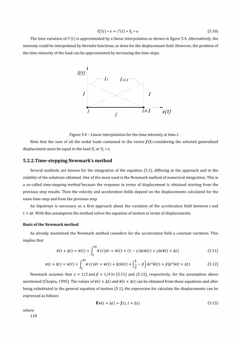
118

��Ü() ∗ � = �Ü() ∗ �� ∗ � (5.10)

The time variation of �Ü() is approximated by a linear interpolation as shown in figure 5.4. Alternatively, the

intensity could be interpolated by Hermite functions, as done for the displacement field. However, the problem of

the time intensity of the load can be approximated by increasing the time steps.

j i+1i

I(t)

x(t)1 1

I i I i+1

Figure 5.4 – Linear interpolation for the time intensity at time t.

Note that the sum of all the nodal loads contained in the vector �(J) considering the selected generalized

displacement must be equal to the load �� or �� ∗ �. 5.2.2.Time-stepping Newmark’s method

Several methods are known for the integration of the equation (5.1), differing in the approach and in the

stability of the solutions obtained. One of the most used is the Newmark method of numerical integration. This is

a so-called time-stepping method because the response in terms of displacement is obtained starting from the

previous step results. Then the velocity and acceleration fields depend on the displacements calculated for the

same time-step and from the previous step.

An hipotesys is necessary as a first approach about the variation of the acceleration field between and + Δ. With this assumption the method solves the equation of motion in terms of displacements. Basis of the Newmark method

As already mentioned the Newmark method considers for the acceleration field a constant variation. This

implies that

:­ ( + Δ) = :­ () + 2 :äN9; (*)3* = :­ () + (1 − ,)Δ:ä () + ,Δ:ä ( + Δ) (5.11)

:( + Δ) = :() + 2 :­N9; (*)3* = :() + Δ:­ () + D12 − �EΔ>:ä () + �Δ>:ä ( + Δ) (5.12)

Newmark assumes that , = 1/2 and � = 1/4 in (5.11) and (5.12), respectively, for the assumption above

mentioned (Chopra, 1995). The values of :­ ( + Δ) and :ä ( + Δ) can be obtained from these equations and after

being substituted in the general equation of motion (5.1), the expression for calculate the displacements can be

expressed as follows

ó�:( + Δ) = �Ã(, + Δ) (5.13)

where

119

ó� = /�Δ> + ,;�Δ + ó (5.14)

�Ã(, + Δ) = �( + Δ) +/G:()�O> + :­ ()�Δ + D 12� − 1E:ä ()H+ ;G ,�Δ :() + D,� − 1E:­ () + Δ D ,2� − 1E:ä ()H

(5.15)

The values of :­ ( + Δ) and :ä ( + Δ) can be calculated in a second phase as functions of the displacement

:( + Δ) or imposing the dynamic equilibrium.

Stability of the method and time step

The constant variation of the acceleration assumption, which is the basis of the Newmark method, provides

an efficient step-by-step integration procedure as long as a short time increment is used. Usually, the time

increment required to achieve an adequate accuracy of the significant response is not unreasonably short

considering that the Newmark method is an unconditionally stable step-by-step method.

In the next numerical example it will be considered for the time step that

Δ ≤ �B100 (5.16)

where �B is the fundamental period of vibration of the structure �B = 1/ÁB expressed in Q-R. Different values of Δ

can be considered to improve the precision of the solution obtained.

5.3. Numerical example

The described modal superposition method can be seen as the method for assembly the solution of a

structural ³-degrees of freedom system in terms of displacements through the solution of a set of ³ independent

SDOF partial differential equations, written in terms of modal coordinates. A numerical example of a three-spans

bridge is presented in the following section. The geometry in the longitudinal direction is the same of the

example 4.6 represented in figure 4.23, being considered the bridge decks represented in figure 4.24 and figure

4.25 for comparison purposes. The bridge deck properties are described in Table 4.12.

5.3.1.Actions on the bridge and structural properties

In railway bridge design there are two essential types of loads involved, the general actions and the rail

traffic actions.

The general actions acting on structures are defined in the EN 1991 (Part 1) and they include the so-called

quasi-permanent loads (Parts 1-1 to 1-6) and the accidental actions (1-7) acting as static loads.

The rail traffic actions with all the action effects are described by the EN 1991 (Part 2). The rail traffic loads

are proposed by alternative models for railway loadings, being the dynamical and centrifugal effects considered

specifically.

In the design of bridges for high speed trains all these loads must be taken into account and the present

analysis considers only a simplified model. The track structure interaction should be considered but it will not be

the object of the present study.

120

The general actions considered are the densities and the self-weight of imposed loads for railway bridges

and are shown in Table 5.1.

Table 5.1 – General actions of the railway bridge.

Action Load magnitude

Self-weight per unit volume (C30/37) [°³/��] 25

Permanent loads [°³/�] 85

Note that the permanent loads presented in Table 5.1 include:

• Ballast;

• Track + Sleepers;

• Post and catenary;

• Concrete blocks for posts;

The concentrated vertical force �� considered as railway action has a magnitude of 1000 °³ and an

eccentricity of 2.5 �. A layout type of the bridge cross-section is proposed as an example in figure 5.5 for a closed

box section.

Figure 5.5 – Bridge layout of the cross-section and sketch of the actions considered.

The structural properties of the bridge decks analyzed are summarized in table 4.13 and the concrete type

considered is the C30/37.

121

5.3.2.Undamped free-vibration analysis

The undamped free-vibration analysis is performed considering the FEM model of the structure and by the

numerical solution of the corresponding eigenvalue problem is possible to obtain the vibration modes and the

respective modal frequencies. The free-vibrating undamped motion refers to both open and closed bridge cross-

section.

Not all the vibration modes will be considered as relevant for the analysis: the EN 1990-A2 refers that the

frequencies until 30 �� should be considered in the dynamic analysis of the bridge.

Note that the mass of the bridge is defined by the general actions specified in Table 5.1 and the element

stiffness and mass matrices used are illustrated by the equations (4.34) and (4.53), respectively.

Open section

For the open double-T bridge section the modal vibration analysis and respective modal frequency are listed

in table 5.2.

Table 5.2 – Undamped vibration modes and respective modal frequencies for the double-T bridge section.

Mode number Frequency [Hz] Major modal participation

1 3.97 Bending motion in (x,z) plan

2 6.49 Bending motion in (x,z) plan

3 7.46 Coupled lateral (y)- torsional (φ) motion

4 7.79 Bending motion in (x,z) plan

5 9.08 Axial motion

6 11.81 Coupled lateral (y)- torsional (φ) motion

7 13.96 Coupled lateral (y)- torsional (φ) motion

8 14.84 Bending motion in (x,z) plan

9 16.53 Coupled lateral (y)- torsional (φ) motion

10 22.51 Bending motion in (x,z) plan

11 24.55 Bending motion in (x,z) plan

12 26.03 Coupled lateral (y)- torsional (φ) motion

13 26.33 Coupled lateral (y)- torsional (φ) motion

14 27.25 Axial motion

15 31.71 Coupled lateral (y)- torsional (φ) motion

As expectable, the first two modes are flexural modes and only the third mode is a torsional mode. Note that

torsion and displacement in the vertical direction are uncoupled, while the �-displacement is coupled with the

twist rotation. Note also that the higher frequencies correspond to much lateral-torsional vibration modes.

The vibration modes for the double-T bridge section are shown in table 5.3 until the 6th mode. Notice that

when the lateral-torsional modes are considered, they cannot be shown by a single graph. In fact, the mode

shape is defined by the coupling between the lateral and torsional displacements and both must be represented

(modes 3 and 6).

122

Table 5.3 – Vibration modes for the double-T bridge section (frequencies in [Hz]).

1 Bending motion in (x,z) plan 2 Bending motion in (x,z) plan

3 Coupled lateral (y)- torsional (φ) motion 4 Bending motion in (x,z) plan

5 Axial motion 6 Coupled lateral (y)- torsional (φ) motion

Notice that the lateral-torsional vibration modes of the continuous beam have different shapes if compared

with those obtained in table 4.19 because of the different proportionality between the lateral and the central

span. The ratio used in the case of table 5.3 is commonly used in real bridge models.

Closed section

The closed-section, which has the properties represented in Table 4.12, have been analyzed in order to

obtain the main vibration modes for the same structure layout, being the results for the first 16 modes with the

respective frequencies represented in table 5.4.

0 10 20 30 40 50 60 70 80 90 100

-2

0

2

x 10-3

Mode number: 1Mode frequency:3.9704

0 10 20 30 40 50 60 70 80 90 100

-1

0

1

x 10-3

Mode number: 2Mode frequency:6.4887

Displacement of the4 d.o.f

0 10 20 30 40 50 60 70 80 90 100

-5

0

5

x 10-4

Mode number: 3Mode frequency:7.4627

Displacement of the2 d.o.f

0 10 20 30 40 50 60 70 80 90 100

-5

0

5

x 10-4

Mode number: 3Mode frequency:7.4627

0 10 20 30 40 50 60 70 80 90 100

-1

0

1

x 10-3

Mode number: 4Mode frequency:7.786

0 10 20 30 40 50 60 70 80 90 100

0

0.5

1

x 10-3

Mode number: 5Mode frequency:9.083

Displacement of the1 d.o.f

0 10 20 30 40 50 60 70 80 90 100

-5

0

5

x 10-4

Mode number: 6Mode frequency:11.8116

0 10 20 30 40 50 60 70 80 90 100

-5

0

5

x 10-4

Mode number: 6Mode frequency:11.8116

Displacement of the6 d.o.f

123

Table 5.4 – Undamped vibration modes and respective modal frequencies for the box bridge section.

Mode number Frequency [Hz] Major modal participation

1 3.79 Bending motion in (x,z) plan

2 6.19 Bending motion in (x,z) plan

3 7.43 Bending motion in (x,z) plan

4 9.08 Axial motion

5 12.05 Coupled lateral (y)- torsional (φ) motion

6 14.16 Bending motion in (x,z) plan

7 15.37 Coupled lateral (y)- torsional (φ) motion

8 16.12 Coupled lateral (y)- torsional (φ) motion

9 16.54 Coupled lateral (y)- torsional (φ) motion

10 21.50 Bending motion in (x,z) plan

11 23.44 Bending motion in (x,z) plan

12 24.56 Coupled lateral (y)- torsional (φ) motion

13 26.02 Coupled lateral (y)- torsional (φ) motion

14 27.25 Axial motion

15 29.52 Coupled lateral (y)- torsional (φ) motion

16 30.70 Bending motion in (x,z) plan

As can be verified from the table 5.4, also in the case of closed section, the first three modes correspond to

the bending in the vertical plane, while the first lateral-torsional motion mode only appears as the 5th vibration

mode.

5.3.3.Forced-vibrations analysis and mode-superposition procedure

In the current analysis the dynamic response of the bridge structure will be obtained by the modal

superposition method. The vibration of the system is forced by a moving load �� with magnitude of 1000°³

travelling at constant speed. The vertical load is applied eccentrically and the eccentricity value is 2.5m, which is

considered according to the tracks position (figure 5.5). The influence of damping is considered for the two

sections studied and for each one of them a damping matrix will be obtained considering the orthogonality

conditions.

Conditions for damping orthogonality

The damping matrix is obtained considering the undamped mode frequencies and the orthogonality

property of the Rayleigh method.

Two different cross-section layouts are compared and for this reason two different damping matrices will be

calculated. The bridge has a 40m central span length and considering the coefficient results for existing bridges

represented in figure 5.2 a damping ratio 0.01 (1%) will be adopted for the 1st and for the 6th bending modes in

the vertical plan. This allows to define numerically the Rayleigh coefficients AB and A> described in the equation

(5.7) as shown in table 5.5.

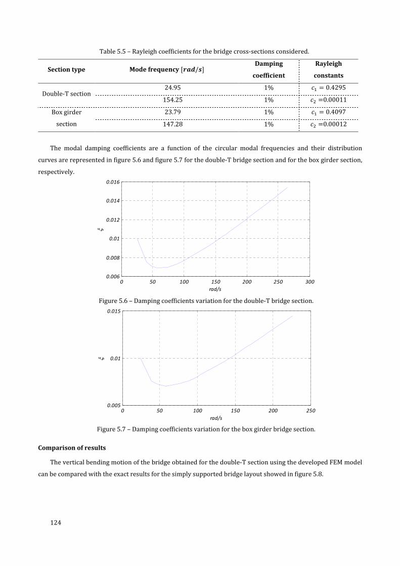
124

Table 5.5 – Rayleigh coefficients for the bridge cross-sections considered.

Section type Mode frequency Q�Pþ/QR Damping

coefficient

Rayleigh

constants

Double-T section 24.95 1% AB = 0.4295

154.25 1% A> =0.00011 Box girder

section

23.79 1% AB = 0.4097 147.28 1% A> =0.00012

The modal damping coefficients are a function of the circular modal frequencies and their distribution

curves are represented in figure 5.6 and figure 5.7 for the double-T bridge section and for the box girder section,

respectively.

Figure 5.6 – Damping coefficients variation for the double-T bridge section.

Figure 5.7 – Damping coefficients variation for the box girder bridge section.

Comparison of results

The vertical bending motion of the bridge obtained for the double-T section using the developed FEM model

can be compared with the exact results for the simply supported bridge layout showed in figure 5.8.

0 50 100 150 200 250 3000.006

0.008

0.01

0.012

0.014

0.016

rad/s

ξ

Variation of the damping coefficient:double-T bridge section

0 50 100 150 200 2500.005

0.01

0.015

rad/s

ξ

Variation of the damping coefficient:box-girder bridge section

125

C

z

y

PZ

L

A

A'

Section AA'

PZ

Figure 5.8 – Layout of the simply supported beam and moving load.

The bridge cross-section of the analysis is the double-T section, which properties are given in table 4.12,

being the length considered for the span � = 40�. At a first approach the undamped motion of the bridge will be considered. The mid-span dimensionless

vertical displacement can be obtained as a function of the considered Ø-vibration mode and of the corresponding

dimensionless velocity, given as follows

= ss(B) = ããCR (5.17)

where s(Û) = S*¡Æ kÎ#T ؽ is the circular frequency of the Ø-vibration mode, s is the load frequency, ã is the load

velocity and ãCR = >È(U)¡Û is the critical structure velocity, defined for the first mode as ãCR = 2Á(B)� for Á(Û) = í(U)>S .

For ≠ Ø and considering only the first vibration mode (Ø = 1), the dimensionless displacement at mid-span (� = �/2) gives

��(�, )��; = sin ð2 1(1 − >) �sin s − sin s(B)� (5.18)

where ��; = �#¡'½&kÎ# is the static displacement of the simply supported beam.

For = Ø = 1 the displacement is given as follows

��(�, )��; = 12 (sin s − s cos s) sin ð2 (5.19)

The results for three characteristics values of are shown in figure 5.9, figure 5.10 and figure 5.11, where the

values obtained from the developed model are successfully compared with the results obtained by (Fryba, 1999).

In table 5.6 is listed the fundamental frequency, the period and the time interval ∆ used for the Newmark

integration.

Table 5.6 – Properties of the simply supported beam-like bridge discretization. Á(B) Q�R 3.5 �(B) Q-R 0.29

∆ QsR 0.003

Number of finite elements 100

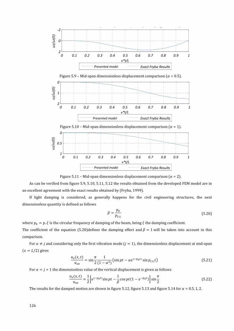
126

Figure 5.9 – Mid-span dimensionless displacement comparison ( = 0.5).

Figure 5.10 – Mid-span dimensionless displacement comparison ( = 1).

Figure 5.11 – Mid-span dimensionless displacement comparison ( = 2).

As can be verified from figure 5.9, 5.10, 5.11, 5.12 the results obtained from the developed FEM model are in

an excellent agreement with the exact results obtained by (Fryba, 1999).

If light damping is considered, as generally happens for the civil engineering structures, the next

dimensionless quantity is defined as follows

� = s8s(B) (5.20)

where s8 = s. � is the circular frequency of damping of the beam, being � the damping coefficient.

The coefficient of the equation (5.20)defines the damping effect and � = 1 will be taken into account in this

comparison.

For ≠ Ø and considering only the first vibration mode (Ø = 1), the dimensionless displacement at mid-span (� = �/2) gives

��(�, )��; = sin ð2 1(1 − >) �sin s − �(úíW9) sin s(B)� (5.21)

For = Ø = 1 the dimensionless value of the vertical displacement is given as follows

��(�, )��; = 12 «�(úíW9)sin s − 1� cos s(1 − �úíW9)¬ sin ð2 (5.22)

The results for the damped motion are shown in figure 5.12, figure 5.13 and figure 5.14 for = 0.5, 1, 2.

0 0.1 0.2 0.3 0.4 0.5 0.6 0.7 0.8 0.9 1

-2

0

2

Dimensionless mid-span z-displacement,α=0.5 (no damping considered)

v*t/L

uz/

uz(

0)

F.E.M. Fryba Results Exact Fryba Results

0 0.1 0.2 0.3 0.4 0.5 0.6 0.7 0.8 0.9 1

0

1

2

Dimensionless mid-span z-displacement, =1 (no damping considered)

v*t/L

uz/

uz(

0)

F.E.M. Fryba Results Exact Fryba Results

0 0.1 0.2 0.3 0.4 0.5 0.6 0.7 0.8 0.9 1

0

0.5

1

Dimensionless mid-span z-displacement, =2 (no damping considered)

v*t/L

uz/

uz(

0)

F.E.M. Fryba Results Exact Fryba Results

Presented model

Presented model

Presented model

127

Figure 5.12 - Mid-span dimensionless displacement comparison ( = 0.5, � = 0.1).

Figure 5.13 - Mid-span dimensionless displacement comparison ( = 1, � = 0.1).

Figure 5.14 - Mid-span dimensionless displacement comparison ( = 2, � = 0.1).

Also in the case in which light damping is considered (� ≪ 1) the accuracy of the results obtained by using

the mode superposition method is sufficiently good. Note that the same quantities listed in table 5.6 are used in

the approximation of the current analysis. The effect of damping in this case is not so influent in terms of

normalized displacements, being the influence lines obtained with � = 0.1 similar to the obtained considering

the undamped motion.

Analysis of the three-span bridge dynamic response

The three spans bridge model with the two cross-section sketched in Figure 5.15 is analysed. The cross-

section dimensions are represented in table 4.12. This section deals with the study of the dynamic response of

the beam-like bridge decks when acted by a vertical and eccentric moving load also shown in Figure 5.15. The

load magnitude is considered constant in time and space and the load motion is assumed to be at a constant

speed.

0 0.1 0.2 0.3 0.4 0.5 0.6 0.7 0.8 0.9 1

-2

0

2

Dimensionless mid-span z-displacement,α=0.5 (β=0.1)

v*t/L

uz/

uz(

0)

F.E.M. Fryba Results Exact Fryba Results

0 0.1 0.2 0.3 0.4 0.5 0.6 0.7 0.8 0.9 1

0

1

2

Dimensionless mid-span z-displacement,α=1 (β=0.1)

v*t/L

uz/

uz(

0)

F.E.M. Fryba Results Exact Fryba Results

0 0.1 0.2 0.3 0.4 0.5 0.6 0.7 0.8 0.9 1

-1

0

1

v*t/L

uz/

uz(

0)

F.E.M. Fryba Results Exact Fryba ResultsPresented model

Presented model

Presented model

128

C

z

y

z

y

ePZ

C

ePZ

4030 30

z

PZ=1000kN

x

v

A'

A

Section AA'

Figure 5.15 – Longitudinal beam-like model (a) and layout of the cross-section analyzed (b).

The eccentricity considered in the numerical example is also constant and its value is fixed to � = 2.5�

because the distance between the vertical axis and the train tracks is imposed from the bridge deck section type

(figure 5.5).

The dynamic behavior of the beam-like bridge is investigated for a set of five different speed values of the

load, considering a maximum speed of 350 km/h that corresponds to a design speed of 420 km/h for high speed

railway bridges. The velocity values considered as an example to obtain influence lines are shown in Table 5.7.

Table 5.7 – Set of train velocities considered.

Train velocities [km/h]

200

250

300

350

420

The dynamic influence of the following kinematic quantities will be analyzed:

• Vertical displacement �� at mid-span (section AA’ of figure 5.15)

• Horizontal transversal displacement �� at mid-span (section AA’ of figure 5.15)

• Twist angle � at mid-pan(section AA’ of figure 5.15)

The results in terms of the dynamic influence lines for the mid-span (AA’) displacements are represented in

figure 5.16, figure 5.17 and figure 5.18 for the double-T open bridge section. Note that the numerical parameters

used in the current analysis relative to the time integration and the FEM model are detailed in table 5.8.

129

Table 5.8 – Parameters considered for the numerical simulation of the current analysis.

Number of finite elements

Lateral span L=30m 75

Middle-span L=40m 100

Lateral span L=30m 75

Time integration interval ∆ QsR= �(B)/200

Vibration modes considered Double-T section 15

Box Girder section 16

Figure 5.16 – Dynamic influence lines of the displacement uz at the section AA’ (double-T section).

Figure 5.17 - Dynamic influence lines of the twist φ at the section AA’ (double-T section).

-1.50

-1.00

-0.50

0.00

0.50

1.00

1.50

2.00

2.50

0 10 20 30 40 50 60 70 80 90 100

uz

[mm

]

x[m]

v=200 km/h

v=250 km/h

v=300 km/h

v=350 km/h

v=420 km/h

-0.06

-0.01

0.04

0.09

0.14

0 10 20 30 40 50 60 70 80 90 100

φQrad*E-03

R x[m]

v=200 km/h

v=250 km/h

v=300 km/h

v=350 km/h

v=420 km/h

130

Figure 5.18 - Dynamic influence lines of the displacement uy at the section AA’ (double-T section).

The dynamic influence lines can be seen as an index of the flexibility of a structure when subjected to a

moving load in the considered direction. The maximum mid-span vertical displacement is obtained for speed

values of 300 km /h and 350 km /h.

Notice the different behavior of the bridge horizontal displacement (figure 5.18) and the twist angle(figure

5.17) from the vertical displacements (figure 5.16). In fact, the �� and � influence lines present functions with

much more oscillations, due to the higher frequencies of the respective vibration modes, if are compared with

the vertical displacement ��, which has a modal contribute with lower frequency.

The effect of warping characterizes the torsional response of the double-T section shape as represented in

figure 5.17, where significant variations of the twist angle values at the section 66’ result from different load

positions along the beam axis.

Table 5.8 shows the limit to the number of vibration modes analyzed considering a maximum frequency of

30 Hz. This assumption reduces the influence of the numerical noise in the results obtained for the model in

analysis.

The figure 5.19,figure 5.20 and figure 5.21 represent the functions obtained for the displacements ��,�� and

for the rotation �, respectively, when the box girder section is considered

Figure 5.19 - Dynamic influence lines of the displacement uz at the section AA’(box girder section)..

-0.13

-0.11

-0.09

-0.07

-0.05

-0.03

-0.01

0.02

0.04

0 10 20 30 40 50 60 70 80 90 100

uy

[mm

]

x[m]

v=200 km/h

v=250 km/h

v=300 km/h

v=350 km/h

v=420 km/h

-1.70

-0.70

0.30

1.30

2.30

3.30

0 10 20 30 40 50 60 70 80 90 100

uz

[mm

]

x[m]

v=200 km/h

v=250 km/h

v=300 km/h

v=350 km/h

v=420 km/h

131

Figure 5.20 - Dynamic influence lines of the twist φ at the section AA’ (box girder section).

Figure 5.21 - Dynamic influence lines of the displacement uy at the section AA’ (box girder section).

The vertical deflections of the box section are similar to those obtained for the open section, being the inertia

of these sections in vertical plan of the same order of magnitude (Figure 5.19). The figure 5.22 presents a further

comparison between the two cross-sections for the vertical displacement influence lines.

Figure 5.22 – Displacement �� for the two bridge sections analyzed (load speed: 420 km/h).

The torsional response represented by the influence line of figure 5.20 allows to conclude that a box girder

has much more torsional stiffness when compared with the double-T section. In fact, figure 5.20 shows that the

dynamic influence line tends to the static influence line for the twist of the section. The horizontal displacements

(figure 5.21) of the box girder sections are less important, in terms of the respective magnitude, if compared with

those of the double-T section. The response in the horizontal direction presents a different sign of the �� if

compared to that of the open bridge section. This effect is probably due to the consideration of the shear strain

-0.02

0

0.02

0.04

0.06

0.08

0 10 20 30 40 50 60 70 80 90 100

φ[r

ad

*E-0

3]

x[m]

v=200 km/h

v=250 km/h

v=300 km/h

v=350 km/h

v=420 km/h

-0.02

-0.01

0.01

0.02

0.03

0.04

0.05

0 10 20 30 40 50 60 70 80 90 100

uy

[mm

]

x [m]

v=200 km/h

v=250 km/h

v=300 km/h

v=350 km/h

v=420 km/h

-1.70

-0.70

0.30

1.30

2.30

3.30

0 10 20 30 40 50 60 70 80 90 100

uz

[m]

x[m]

Comparison of bridge sections: train speed 420 km/h

Box Girder Section

Double-T section

132

included in the sectorial coordinate, according to (Benscoter, 1954): for the box-girder section layout the shear

centre assumes a different position, being the sign of (C − ¢) opposite to that of the open double-T section. This different effect on the horizontal displacement of the two section-types analyzed is shown by figure 5.23 for the

fixed value of maximum train speed analyzed: v=420 km/h.

Figure 5.23 – Horizontal displacements of the bridge cross-section(load speed: 420 km/h).

Figure 5.24 - Twist of the bridge sections (load speed: 420 km/h).

The torsional response is completely different for the two section types (Figure 5.24). As expectable, the

closed section twist only reaches high values for the loading positioned at the central span, while the open

section, more affected by warping, presents high values of rotation for a load located at the external spans.

The maximum displacement and twist rotation � at the section 66’ can also be plotted as functions of the

load speed values. These curves are shown in figure 5.25 and figure 5.26 for the double-T and for the box girder

bridge sections.

-0.12

-0.1

-0.08

-0.06

-0.04

-0.02

0

0.02

0.04

0 10 20 30 40 50 60 70 80 90 100

uy

[mm

]

x [m]

Box girder section

Double-T section

-0.06

-0.03

0

0.03

0.06

0.09

0.12

0.15

0 10 20 30 40 50 60 70 80 90 100

φ[r

ad

*E-0

3]

x [m]

Box girder section

Double-T section

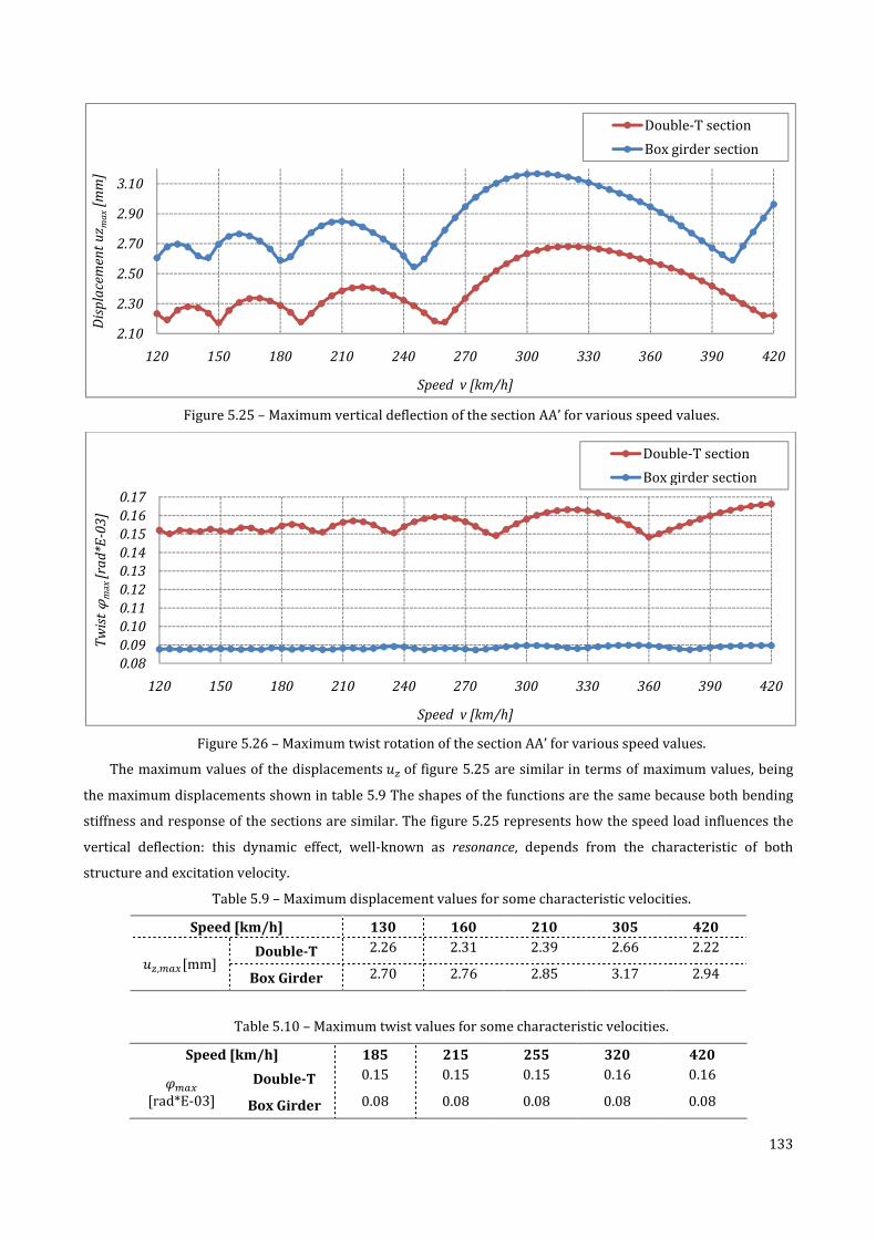
133

Figure 5.25 – Maximum vertical deflection of the section AA’ for various speed values.

Figure 5.26 – Maximum twist rotation of the section AA’ for various speed values.

The maximum values of the displacements �� of figure 5.25 are similar in terms of maximum values, being

the maximum displacements shown in table 5.9 The shapes of the functions are the same because both bending

stiffness and response of the sections are similar. The figure 5.25 represents how the speed load influences the

vertical deflection: this dynamic effect, well-known as resonance, depends from the characteristic of both

structure and excitation velocity.

Table 5.9 – Maximum displacement values for some characteristic velocities.

Speed [km/h] 130 160 210 305 420

��,Ӣ$[mm] Double-T 2.26 2.31 2.39 2.66 2.22

Box Girder 2.70 2.76 2.85 3.17 2.94

Table 5.10 – Maximum twist values for some characteristic velocities.

Speed [km/h] 185 215 255 320 420 �Ó¢$ [rad*E-03]

Double-T 0.15 0.15 0.15 0.16 0.16

Box Girder 0.08 0.08 0.08 0.08 0.08

2.10

2.30

2.50

2.70

2.90

3.10

120 150 180 210 240 270 300 330 360 390 420

Dis

pla

cem

ent

uz m

ax

[mm

]

Speed v [km/h]

Double-T section

Box girder section

0.08

0.09

0.10

0.11

0.12

0.13

0.14

0.15

0.16

0.17

120 150 180 210 240 270 300 330 360 390 420

Tw

ist

φ max[ra

d*E

-03

]

Speed v [km/h]

Double-T section

Box girder section

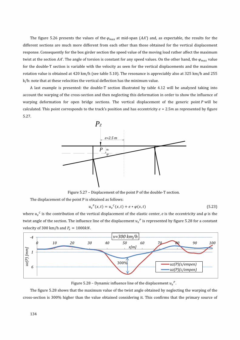
134

The figure 5.26 presents the values of the �Ó¢$ at mid-span (66’) and, as expectable, the results for the

different sections are much more different from each other than those obtained for the vertical displacement

response. Consequently for the box girder section the speed value of the moving load rather affect the maximum

twist at the section 66’. The angle of torsion is constant for any speed values. On the other hand, the �Ó¢$ value

for the double-T section is variable with the velocity as seen for the vertical displacements and the maximum

rotation value is obtained at 420 km/h (see table 5.10). The resonance is appreciably also at 325 km/h and 255

k/h: note that at these velocities the vertical deflection has the minimum value.

A last example is presented: the double-T section illustrated by table 4.12 will be analyzed taking into

account the warping of the cross-section and then neglecting this deformation in order to show the influence of

warping deformation for open bridge sections. The vertical displacement of the generic point � will be

calculated. This point corresponds to the track’s position and has eccentricity � = 2.5� as represented by figure

5.27.

Figure 5.27 – Displacement of the point P of the double-T section.

The displacement of the point P is obtained as follows:

���(�, ) = ��Å(�, ) + � ∗ �(�, ) (5.23)

where ��Šis the contribution of the vertical displacement of the elastic center, � is the eccentricity and � is the

twist angle of the section. The influence line of the displacement ��� is represented by figure 5.28 for a constant

velocity of 300 km/h and �� = 1000°³.

Figure 5.28 – Dynamic influence line of the displacement ��� .

The figure 5.28 shows that the maximum value of the twist angle obtained by neglecting the warping of the

cross-section is 300% higher than the value obtained considering it. This confirms that the primary source of

e=2.5 m

Z

Pϕ

uz

-4

1

6

0 10 20 30 40 50 60 70 80 90 100

uz(

P)

[mm

] x[m]

v=300 km/h

uz(P)(s/empen)

uz(P)(c/empen)

300%

135

torsion resistance, in the case of open sections, is the warping stiffness and the error in estimating the dynamic

displacements is greatly affected by its consideration.

137

6. CONCLUSIONS AND FINITE DEVELOPMENTS

6.1. General remarks

The introduction of this thesis stated that the main objective of this work was to investigate one-dimensional

thin-walled beam-like structures for arbitrary geometry of the cross-section, loading cases and boundary

conditions and to enable an accurate representation of the widest range possible of behaviors in static and

dynamics.

The analysis performed in this work is focused on the consideration of the torsional response of both open

and closed cross-sections of thin-walled beams. For this reason a finite element model with seven degrees of

freedom for each end has been formulated and implemented through a numerical code.

The target was reached; all the designed and developed models gave satisfactory results and were

conclusive. The work has provided important information that enhances the understanding of structural

problems and the fundamental physical principles that underlie them related to the cross-section warping. The

model that has been presented allows a simplified analysis of straight thin-walled beam with arbitrary boundary

conditions and generally loaded, both in statics and dynamics. The major propose is the application of this beam

element to the analysis of bridges, in particular in the analysis to moving loads.

6.1. Conclusions

Starting from the governing differential equations of the axial, bending and torsional effects and considering

the Euler Bernoulli and Vlasov thin-walled beam theories, a finite element formulation has been developed

according to variational principles.

The whole beam element with arbitrary thin-walled cross-section was represented by its elastic center axis

and Hermite polynomials were used as approximation functions of the displacement field. For this discrete

element the stiffness and mass matrices and the vector of external loads were derived without neglecting terms.

In statics, basic examples of generally loaded beams with different cross-sectional behaviors have been

presented for the understanding of the influence of warping in the displacement field and stress analysis. The

exact results obtained by (Kollbrunner & Basler, 1969) have been simulated in order to check the accuracy of the

obtained solution. Also a comparison with ABAQUS has been performed in order to check the stiffness method

developed in the work.

The focus of these comparisons has been based on the following aspects:

• The consideration of a C, I and hollow cross-section;

• Two types of simply supported structures: a simply supported beam and a three continuous spans

beam;

• Two types of loading: a concentrated and an uniformly distributed torque.

A study of convergence has been presented for the finite element model developed by increasing the

elements of the mesh until it was reached a sufficiently good approximation. Also two sections, a double-T and a

closed box, of a three-span bridge layout have been studied, being the lateral-torsional response obtained in

terms of displacements and forces.

138

In dynamics, the following three structural behaviors have been investigated:

• The free torsional vibrations of generally supported beams. In this case, the results have been

compared with those obtained by (Gere, 1954) for I-sections and the influence of warping and

boundary conditions in the modal frequency values is studied;

• The forced vibrations of generally supported beams acted by a moving vertical load at constant

velocity. The results have been compared with the exact solution of (Fryba, 1999) for the simple

case of a load acting in the vertical plane without eccentricity;

• The effect of an eccentric vertical load in the lateral-torsional and flexural response of a straight

beam with continuous spans. The bridge sections considered were a double-T girder and a box

girder with two lanes.

The modal superposition method has been used in order to obtain the structural response and obtain

dynamic influence lines for the thin-walled beams analyzed. In dynamics, the comparison between the two cross-

sections mentioned has been performed. The bridge model response confirmed that the warping deformation

greatly affects its behavior when the open section is considered.

The differences in terms of twist angle and lateral displacements, obtained for a set of different load speeds,

between the box section and the open section has allowed to verify that warping is fundamental to a correct

analysis of these structural element types.

6.2. Future developments

As already known from the Saint Venant theory, the closed sections warp much less than open thin walled

sections and for this reason the classic Euler-Bernoulli beam element neglects the warping deformability.

Therefore these elements are commonly used by the most known structural software such SAP, or ADINA.

Other simulation codes, such the ANSYS or the ABAQUS, allow to use elements with seven degrees of

freedom, but the use of these tools are more adequate to the study of buckling and connection problems and its

understanding is not so simple at a first approach.

The presented model could be considered as the first step tending to a more complete formulation

accounting for several aspects that have not yet been considered, listed as follows:

• The addition of the Benscoter’s consideration of the distorsion in the degrees of freedom of the finite

element, which is an important aspect in the analysis of box girder bridge sections;

• The variation of the cross-section height along the beam axis, important specially for the analysis of

open bridge sections because of the high values of the hogging moments on the bearing sections;

• The consideration of curved bridges in plane, with arbitrary types of cross-sections;

• The compatibility with the Eurocodes relative to the rail traffic model that should be considered as

traffic loads. This aspect involves the consideration of load models more complex than the simple

load considered by the analysis, i.e. the load models for real trains(HSLM10 model);

• Consideration of track-structure interactions that must be taken into account according to the EN

1991-2.

10 High Speed Load Model.

139

• The consideration of support conditions defined at the real point of their applications, i.e. the

bearings of a real multi-span bridges at the pier sections.

141

7. References

Benscoter, S. (1954). A theory of torsion bending for multicell beams. Journal of Applied Mechanics , 25-34.

Cedolin, L. (1996). Torsione e taglio di travi a parete sottile. Milano: Edizioni Cusl.

Chopra, A. (1995). Dynamics of Structures- Theory and application to the Earthquake Engineering. Berkeley:

Prentice Hall,Inc.

Clough, R., & Penzien, J. (1982). Dynamics of structures. McGraw-Hill.

Cunha, R. (2007). Dinâmica de Pontes em Viga Caixão em Linhas Ferroviárias de Alta Velocidade (Master

Thesis). FEUP. (p-40). Dinâmica de Pontes em Viga Caixão em Linhas Ferroviárias de Alta Velocidade (Master

Thesis). FEUP. (p-40) . Porto.

Ferreira, A. (2010). Problemas De Elementos Finitos em Matlab. Lisbon: Fundação Calouste Gulbenkian.

Fish, J., & Belytschko, T. (2007). A First Course In Finite Elements. John Wiley & Sons Ltd.

Friberg, P. (1985). Beam element matrices derived from Vlasov's theory of open thin-walled elastic beams .

International Journal for Numerical Methods in Engineering , 1206-1218.

Fryba, L. (1999). Simply supported beam subjected to a moving constant force. In L. Fryba, Vibration of Solids

and Structures under Moving Loads (third edition) (pp. 13-56). Prague: Thomas Telford Ltd.

Gere, J. (1954). Torsional Vibrations of Beams of Thin-Walled Open Section. Journal Of Applied Mechanics ,

381-387.

Hibbit, K. a. (2007). ABAQUS users manual version 6.7. U.S.A., U.S.A.

Kollbrunner, C., & Basler, K. (1969). Torsion in Structures: An Engineering Approach. In C. Kollbrunner, & K.

Brasler, Kollbrunner,C.F.;Brasler,K. (pp. 158-200). Springer.

Michaltos, G., Sarantithou, E., & Sophianopoulos, D. (2003). Flexural-torsional vibration of simply supported

open cross-section steel beams under moving loads. Journal of Sound and Vibrations , 480-494.

Okeil, A., & S., E.-T. (2004). Warping stresses in curved box girder bridges:case study. . Journal of Bridge

Engineering , 487-496.

Prokić, A. (2003). On triply coupled vibrations of thin-walled beams with arbitrary cross-section. Journal of

Sound and Vibration , 723-737.

Prokić, A. (2002). Stiffness method of thin-walled beams with closed cross-section. Computers and Structures

, 40-51.

Prokić, A., & Lukić, D. (2007). Dynamic analysis of thin-walled closed-section beams . Journal of Sound and

Vibration , 963-980.

Saadé, K., Espion, B., & Warzée, G. (2003). Non-uniform torsional behavior and stability of thin-walled elastic

beams with arbitrary cross sections. Thin-Walled Structures , 857-881.

Shakourzadeh, H., Guo, Y., & Batoz, J. (1993). A torsion bending element for thin-walled beams with open and

closed cross-sections. Computers and Structures , 1045-1054.

Vlasov, V. (1961). Thin-walled elastic bars (english transl.). Jerusalem.

143

ANNEX 1

In the Annex 1 the cross-section cartesian and sectorial coordinates for the layouts analyzed are represented

referred to the elastic center of the section.

Bb b

tw tw

tfC

z

y

Bb b

htw

tfC

z

y

ab1

E

tf1

E

ba

m

Figure A.0.1 – Cross-section layouts

1/2(2b+B)zc

1/2Bzc

0 -1/2Bzc

-1/2(2b+B)zc

-1/2(zc+h)Bωc

ωE

1/2k1B/tf

0

+k1(1/2B/tf+ba/tw)-1/2hB

1/2hB-k1(1/2B/tf+ba/tw)

1/2k1B/t f

-1/2k1B/t f

-1/2k1B/t f

1/2(zc+h)B

1/2Bh

-1/2Bh ωE

0

zcB/2+bzc-1/2k1B/t f

zcB/2-1/2k1B/t f

zcB/2+bam-k1(1/2B/tf+ba/tw) k1(1/2B/t f+ba/tw)

-zcB/2-bam

1/2k1B/tf -zcB/2-bzc

1/2k1B/t f

-zcB/2

ωc

Figure A.0.2 – Sectorial coordinate for the open and closed cross-sections.

144

-zc

-zc

-zc

-zc

h-zc

h-zc

z-zc

-1/2(2b+B)

0

1/2B

1/2(2b+B)

-1/2b1

1/2b1

-zc

-zc

-zc

-zc

-zc

0

y-yc

z-zch-zc

h-zc

1/2(2b+B)

-1/2(2b+B)

0

1/2B

1/2B

-1/2B

y-yc

Figure A.0.3 – Cartesian coordinates referred to the elastic center.