Yu.I. Bogdanov LANL Report quant-ph/0303014 Root Estimator ... · Yu.I. Bogdanov LANL Report...
26
Yu.I. Bogdanov LANL Report quant-ph/0303014 1 Root Estimator of Quantum States Yu. I. Bogdanov OAO "Angstrem", Moscow, Russia E-mail: [email protected] Abstract The root estimator of quantum states based on the expansion of the psi function in terms of system eigenfunctions followed by estimating the expansion coefficients by the maximum likelihood method is considered. In order to provide statistical completeness of the analysis, it is necessary to perform measurements in mutually complementing experiments (according to the Bohr terminology). Estimation of quantum states by the results of coordinate, momentum, and polarization (spin) measurements is considered. The maximum likelihood technique and likelihood equation are generalized in order to analyze quantum mechanical experiments. The Fisher information matrix and covariance matrix are considered for a quantum statistical ensemble. The constraints on the energy are shown to result in high-frequency noise reduction in the reconstructed state vector. Informational aspects of the problem of division a mixture are studied and a special (quasi- Bayesian) algorithm for solving this problem is proposed. It is shown that the requirement for the expansion to be of a root kind can be considered as a quantization condition making it possible to choose systems described by quantum mechanics from all statistical models consistent, on average, with the laws of classical mechanics. Introduction. In the previous paper (“Quantum Mechanical View of Mathematical Statistics” quant- ph/0303013- hereafter, Paper 1), is has been shown that the root density estimator, based on the introducing an object similar to the psi function in quantum mechanics into mathematical statistics, is an effective tool of statistical data analysis. In this paper, we will show that in problems of estimating of quantum states, the root estimators are at least of the same importance as in the problems of classical statistical analysis. Methodologically, the method considered here essentially differs from other well known methods for estimating quantum states that arise from applying the methods of classical tomography and classical statistics to quantum problems [1-3]. The quantum analogue of the distribution density is the density matrix and the corresponding Wigner distribution function. Therefore, the methods developed so far have been aimed at reconstructing the aforementioned objects in analogy with the methods of classical tomography (this resulted in the term “quantum tomography”) [4]. In [5], a quantum tomography technique on the basis of the Radon transformation of the Wigner function was proposed. The estimation of quantum states by the method of least squares was considered in [6]. The maximum likelihood technique was first presented in [7,8]. The version of the maximum likelihood method providing fulfillment of basic conditions imposed of the density matrix (hermicity, nonnegative definiteness, and trace of matrix equal to unity) was given in [9,10]. Characteristic features of all these methods are rapidly increasing calculation complexity with increasing number of parameters to be estimated and ill-posedness of the corresponding algorithms, not allowing one to find correct stable solutions. The orientation toward reconstructing the density matrix overshadows the problem of estimating more fundamental object of quantum theory, i.e., the state vector (psi function). Formally, the states described by the psi function are particular cases of those described by the density matrix. On the other hand, this is the very special case that corresponds to fundamental laws in Nature and is related to the situation when the state described by a large number of unknown parameters may be stable and estimated up to the maximum possible accuracy.
Transcript of Yu.I. Bogdanov LANL Report quant-ph/0303014 Root Estimator ... · Yu.I. Bogdanov LANL Report...

Yu.I. Bogdanov LANL Report quant-ph/0303014
1
Root Estimator of Quantum States
Yu. I. Bogdanov
OAO "Angstrem", Moscow, RussiaE-mail: [email protected]
AbstractThe root estimator of quantum states based on the expansion of the psi function in terms of systemeigenfunctions followed by estimating the expansion coefficients by the maximum likelihoodmethod is considered. In order to provide statistical completeness of the analysis, it is necessary toperform measurements in mutually complementing experiments (according to the Bohrterminology). Estimation of quantum states by the results of coordinate, momentum, andpolarization (spin) measurements is considered. The maximum likelihood technique and likelihoodequation are generalized in order to analyze quantum mechanical experiments. The Fisherinformation matrix and covariance matrix are considered for a quantum statistical ensemble. Theconstraints on the energy are shown to result in high-frequency noise reduction in the reconstructedstate vector. Informational aspects of the problem of division a mixture are studied and a special(quasi- Bayesian) algorithm for solving this problem is proposed. It is shown that the requirementfor the expansion to be of a root kind can be considered as a quantization condition making itpossible to choose systems described by quantum mechanics from all statistical models consistent,on average, with the laws of classical mechanics.
Introduction.In the previous paper (“Quantum Mechanical View of Mathematical Statistics” quant-
ph/0303013- hereafter, Paper 1), is has been shown that the root density estimator, based on theintroducing an object similar to the psi function in quantum mechanics into mathematical statistics,is an effective tool of statistical data analysis. In this paper, we will show that in problems ofestimating of quantum states, the root estimators are at least of the same importance as in theproblems of classical statistical analysis.
Methodologically, the method considered here essentially differs from other well knownmethods for estimating quantum states that arise from applying the methods of classicaltomography and classical statistics to quantum problems [1-3]. The quantum analogue of thedistribution density is the density matrix and the corresponding Wigner distribution function.Therefore, the methods developed so far have been aimed at reconstructing the aforementionedobjects in analogy with the methods of classical tomography (this resulted in the term “quantumtomography”) [4].
In [5], a quantum tomography technique on the basis of the Radon transformation of theWigner function was proposed. The estimation of quantum states by the method of least squareswas considered in [6]. The maximum likelihood technique was first presented in [7,8]. The versionof the maximum likelihood method providing fulfillment of basic conditions imposed of the densitymatrix (hermicity, nonnegative definiteness, and trace of matrix equal to unity) was given in [9,10].Characteristic features of all these methods are rapidly increasing calculation complexity withincreasing number of parameters to be estimated and ill-posedness of the corresponding algorithms,not allowing one to find correct stable solutions.
The orientation toward reconstructing the density matrix overshadows the problem ofestimating more fundamental object of quantum theory, i.e., the state vector (psi function).Formally, the states described by the psi function are particular cases of those described by thedensity matrix. On the other hand, this is the very special case that corresponds to fundamental lawsin Nature and is related to the situation when the state described by a large number of unknownparameters may be stable and estimated up to the maximum possible accuracy.

Yu.I. Bogdanov LANL Report quant-ph/0303014
2
In Sec. 1, the problem of estimating quantum states is considered in the framework of themutually complementing measurements (Bohr [11]). The likelihood equation and statisticalproperties of estimated parameters are studied.
In Sec. 2, the maximum likelihood method is generalized on the case when, along with thecondition on the norm of a state, additional constraint on energy is introduced. The latter restrictionallows one to suppress noise corresponding to the high-frequency range of the spectrum of aquantum state.
In Sec. 3, the problem of reconstructing the spin state is briefly considered. In thenonrelativistic approximation, the coordinate and spin wave functions are factorized; therefore, thecorresponding problems of reconstructing the states can be considered independently in the sameapproximation.
The mixture separation problem is considered in Sec. 4. It is shown that from theinformation standpoint it is purposefully to divide initial data into uniform (pure) sets and performindependent estimation of the state vector for each set. A quasi- Bayesian self-consistent algorithmfor solving this problem is proposed.
In Sec. 5, it is shown that the root expansion basis following from quantum mechanics ispreferable to any other set of orthonormal functions, since the classical mechanical equations aresatisfied for averaged quantities according to the Ehrenfest theorems. Thus, the requirement for theprobability density to be of the root form plays a role of the quantization condition.
1. Phase Role. Statistical Analysis of Mutually Complementing Experiments. StatisticalInverse Problem in Quantum Mechanics.
We have defined in the Paper.1 the psi function as a complex-valued function with thesquared absolute value equal to the probability density. From this point of view, any psi functioncan be determined up to arbitrary phase factor ( )( )xiSexp . In particular, the psi function can bechosen real-valued. For instance, in estimating the psi function in a histogram basis, the phases ofamplitudes (4.2) of the Paper.1, which have been chosen equal to zero, could be arbitrary.
At the same time, from the physical standpoint, the phase of psi function is not redundant.The psi function becomes essentially complex valued function in analysis of mutuallycomplementing (according to Bohr) experiments with micro objects [11].
According to quantum mechanics, experimental study of statistical ensemble in coordinatespace is incomplete and has to be completed by study of the same ensemble in another (canonicallyconjugate, namely, momentum) space. Note that measurements of ensemble parameters incanonically conjugate spaces (e.g., coordinate and momentum spaces) cannot be realized in thesame experimental setup.
The uncertainty relation implies that the two-dimensional density in phase space ( )pxP , isphysically senseless, since the coordinates and momenta of micro objects cannot be measured
simultaneously. The coordinate ( )xP and momentum ( )pP~ distributions should be studiedseparately in mutually complementing experiments and then combined by introducing the psifunction. We will consider the so-called sharp measurements resulting in collapse of the wavefunction (for unsharp measurements, see [12]).
The coordinate-space and momentum-space psi functions are related to each other by theFourier transform ( 1=h )
( ) ( ) ( )∫= dpipxpx exp~21
ψπ
ψ , (1.1)
( ) ( ) ( )∫ −= dxipxxp exp21~ ψπ
ψ . (1.2)
Yu.I. Bogdanov LANL Report quant-ph/0303014
3
Consider a problem of estimating an unknown psi function ( ( )xψ or ( )pψ~ ) byexperimental data observed both in coordinate and momentum spaces. We will refer to this problemas an statistical inverse problem of quantum mechanics (do not confuse it with an inverse problemin the scattering theory). The predictions of quantum mechanics are considered as a direct problem.Thus, we consider quantum mechanics as a stochastic theory, i.e., a theory describing statistical(frequency) properties of experiments with random events. However, quantum mechanics is aspecial stochastic theory, since one has to perform mutually complementing experiments (space-time description has to be completed by momentum-energy one) to get statistically full descriptionof a population (ensemble). In order for various representations to be mutually consistent, the theoryshould be expressed in terms of probability amplitude rather than probabilities themselves.
A simplified approach to the inverse statistical problem, which will be exemplified by
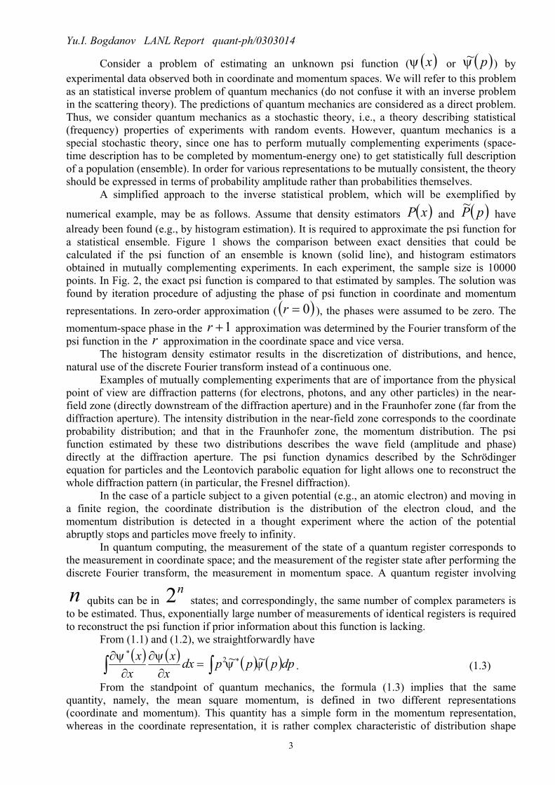
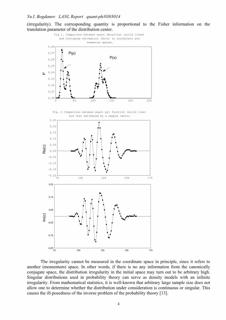
numerical example, may be as follows. Assume that density estimators ( )xP and ( )pP~ havealready been found (e.g., by histogram estimation). It is required to approximate the psi function fora statistical ensemble. Figure 1 shows the comparison between exact densities that could becalculated if the psi function of an ensemble is known (solid line), and histogram estimatorsobtained in mutually complementing experiments. In each experiment, the sample size is 10000points. In Fig. 2, the exact psi function is compared to that estimated by samples. The solution wasfound by iteration procedure of adjusting the phase of psi function in coordinate and momentumrepresentations. In zero-order approximation ( ( )0=r ), the phases were assumed to be zero. Themomentum-space phase in the 1+r approximation was determined by the Fourier transform of thepsi function in the r approximation in the coordinate space and vice versa.
The histogram density estimator results in the discretization of distributions, and hence,natural use of the discrete Fourier transform instead of a continuous one.
Examples of mutually complementing experiments that are of importance from the physicalpoint of view are diffraction patterns (for electrons, photons, and any other particles) in the near-field zone (directly downstream of the diffraction aperture) and in the Fraunhofer zone (far from thediffraction aperture). The intensity distribution in the near-field zone corresponds to the coordinateprobability distribution; and that in the Fraunhofer zone, the momentum distribution. The psifunction estimated by these two distributions describes the wave field (amplitude and phase)directly at the diffraction aperture. The psi function dynamics described by the Schrödingerequation for particles and the Leontovich parabolic equation for light allows one to reconstruct thewhole diffraction pattern (in particular, the Fresnel diffraction).
In the case of a particle subject to a given potential (e.g., an atomic electron) and moving ina finite region, the coordinate distribution is the distribution of the electron cloud, and themomentum distribution is detected in a thought experiment where the action of the potentialabruptly stops and particles move freely to infinity.
In quantum computing, the measurement of the state of a quantum register corresponds tothe measurement in coordinate space; and the measurement of the register state after performing thediscrete Fourier transform, the measurement in momentum space. A quantum register involving
n qubits can be in n2 states; and correspondingly, the same number of complex parameters is
to be estimated. Thus, exponentially large number of measurements of identical registers is requiredto reconstruct the psi function if prior information about this function is lacking.
From (1.1) and (1.2), we straightforwardly have( ) ( ) ( ) ( )∫∫ ∗
∗
=∂
∂∂
∂ dppppdxxx
xx
ψψψψ ~~2 . (1.3)
From the standpoint of quantum mechanics, the formula (1.3) implies that the samequantity, namely, the mean square momentum, is defined in two different representations(coordinate and momentum). This quantity has a simple form in the momentum representation,whereas in the coordinate representation, it is rather complex characteristic of distribution shape
Yu.I. Bogdanov LANL Report quant-ph/0303014
4
(irregularity). The corresponding quantity is proportional to the Fisher information on thetranslation parameter of the distribution center.
Fig 1. Comparison between exact densities (solid lines)
and histogram estimators (dots) in coordinate and
momentum spaces.P
0,00
0,01
0,02
0,03
0,04
0,05
0,06
0,07
0,08
0 50 100 150 200 250
P(p)P(x)
Fig. 2 Comparison between exact psi function (solid line)
and that estimated by a sample (dots).
Re(
c)
-0,20
-0,15
-0,10
-0,05
0,00
0,05
0,10
0,15
0,20
0,25
75 100 125 150 175
Im(c
)
-0,25
-0,15
-0,05
0,05
0,15
0,25
75 100 125 150 175
The irregularity cannot be measured in the coordinate space in principle, since it refers toanother (momentum) space. In other words, if there is no any information from the canonicallyconjugate space, the distribution irregularity in the initial space may turn out to be arbitrary high.Singular distributions used in probability theory can serve as density models with an infiniteirregularity. From mathematical statistics, it is well-known that arbitrary large sample size does notallow one to determine whether the distribution under consideration is continuous or singular. Thiscauses the ill-posedness of the inverse problem of the probability theory [13].

Yu.I. Bogdanov LANL Report quant-ph/0303014
5
Thus, from the standpoint of quantum mechanics, the ill-posedness of the classical problemof density estimation by a sample is due to lack of information from the canonically conjugatespace. Regularization methods for inverse problem consist in excluding a priory strongly-irregularfunctions from consideration. This is equivalent to suppression of high momenta in the momentumspace.
Let us turn now to more consistent description of the method for estimation of the statevector of a statistical ensemble on the basis of experimental data obtained in mutuallycomplementing experiments. Consider corresponding generalization of the maximum likelihoodprinciple and likelihood equation. To be specific, we will assume that corresponding experimentsrelate to coordinate and momentum spaces.
We define the likelihood function as
( ) ( ) ( )∏∏==
=m
jj
n
ii cpPcxPcpxL
11
~, . (1.4)
Here, ( )cxP i and ( )cpP j~
are the densities in mutually complementing experiments
corresponding to the same state vector c . We assume that n measurements were made in thecoordinate space; and m , in the momentum one.
Then, the log likelihood function has the form (instead of (3.1) of the Paper.1)
( ) ( )∑∑==
+=m
jj
n
ii cpPcxPL
11
~lnlnln . (1.5)
The maximum likelihood principle together with the normalization condition evidentlyresults in the problem of maximization of the following functional:
( )1ln −−= ∗iiccLS λ , (1.6)
where λ is the Lagrange multiplier and
( ) ( )( ) ( ) ( )( )∑∑=
∗∗
=
∗∗ +=m
lljliji
n
kkjkiji ppccxxccL
11
~~lnlnln ϕϕϕϕ . (1.7)
Here, ( )piϕ~
is the Fourier transform of the function ( )xiϕ .The likelihood equation has the form similar to (3.7) of the Paper.1.
1,...,1,0, −== sjiccR ijij λ , (1.8)
where the R matrix is determined by( ) ( )
( )( ) ( )
( )∑∑==
+=m
l l
ljlin
k k
kjkiij pP
ppxP
xxR
1
*
1
*
~~~ ϕϕϕϕ
. (1.9)
By full analogy with calculations conducted in Sec.3 of the Paper.1, it can be proved that themost likely state vector always corresponds to the eigenvalue mn +=λ of the R matrix (equalto sum of measurements).
The likelihood equation can be easily expressed in the form similar to (3.10) of the Paper.1:
( )( )
( )( )
i
n
k
m
ls
jljj
lis
jkjj
ki cpc
p
xc
xmn
=
++ ∑ ∑
∑∑= =
=
∗∗
∗
=
∗∗
∗
1 1
11
~
~1
ϕ
ϕ
ϕ
ϕ . (1.10)
The Fisher information matrix (prototype) is determined by the total information containedin mutually complementing experiments (compare to (1.5) and (1.6) of the Paper. 1):
Yu.I. Bogdanov LANL Report quant-ph/0303014
6
( ) ( ) ( ) ( ) ( ) ( ) ( )dpcpPc
cpPc
cpPmdxcxPc
cxPc
cxPncIjiji
ij ,~,~ln,~ln,,ln,ln~∗∗ ∂
∂∂
∂⋅+
∂∂
∂∂
⋅= ∫∫ , (1.11)
( ) ( ) ( ) ( ) ( ) ijjiji
ij mndpc
cpc
cpmdxc
cxc
cxnI δψψψψ
+=∂
∂∂
∂⋅+
∂∂
∂∂
⋅= ∗
∗
∗
∗
∫∫,~,~,,~
. (1.12)
Note that the factor of 4 is absent in (1.12) in contrast to the similar formula (1.6) of the
Paper.1. This is because of the fact that it is necessary to distinguish ( )xψ and ( )x∗ψ as well as
c and ∗c .Consider the following simple transformation of a state vector that is of vital importance
(global gauge transformation). It is reduced to multiplying the initial state vector by arbitrary phasefactor:
( )cic exp α=′ , (1.13)where α is arbitrary real number.
One can easily verify that the likelihood function is invariant against the gaugetransformation (1.13). This implies that the state vector can be estimated by experimental data up toarbitrary phase factor. In other words, two state vectors that differ only in a phase factor describethe same statistical ensemble. The gauge invariance, of course, also manifests itself in theory, e.g.,in the gauge invariance of the Schrödinger equation.
The variation of a state vector that corresponds to infinitesimal gauge transformation isevidently
1,...,1,0 −== sjcic jj αδ , (1.14)where α is a small real number.
Consider how the gauge invariance has to be taken into account in considering statistical
fluctuations of the components of a state vector. The normalization condition ( 1=∗jjcc ) yields that
the variations of the components of a state vector satisfy the condition( ) 0=+ ∗∗
jjjj cccc δδ . (1.15)
Here, jjj ccc −= ˆδ is the deviation of the state estimator found by the maximumlikelihood method from the true state vector characterizing the statistical ensemble.
In view of the gauge invariance, let us divide the variation of a state vector into two termsccc 21 δδδ += . The first term cic 1 αδ = corresponds to gauge arbitrariness, and the second
one c2δ is a real physical fluctuation.An algorithm of dividing of the variation into gauge and physical terms can be represented
as follows. Let cδ be arbitrary variation meeting the normalization condition. Then, (1.15) yields
( ) εδ icc jj =∗, where ε is a small real number.
Dividing the variation cδ into two parts in this way, we have( ) ( ) ( ) εδαδαδ iccicccicc jjjjjjj =+=+= ∗∗∗
22 . (1.16)Choosing the phase of the gauge transformation according to the condition εα = , we find
( ) 02 =∗jj ccδ . (1.17)
Let us show that this gauge transformation provides minimization of the sum of squares of
variation absolute values. Let ( ) εδ icc jj =∗. Having performed infinitesimal gauge transformation,
we get the new variation

Yu.I. Bogdanov LANL Report quant-ph/0303014
7
jjj ccic δαδ +−=′ . (1.18)Our aim is to minimize the following expression:
( )( ) min2 2 →+−=++−=′′ ∗∗∗∗ αεαδδδαδαδδ jjjjjjjj cccciccicc . (1.19)Evidently, the last expression has a minimum at εα = .
Thus, the gauge transformation providing separation of the physical fluctuation from thevariation achieves two aims.
First, the condition (1.15) is divided into two independent conditions:
( ) 0=∗jj ccδ and ( ) 0=∗
jj ccδ (1.20).Here, we have dropped the subscript 2 assuming that the state vector variation is a physical
fluctuation free of the gauge component).Second, this transformation results in mean square minimization of possible variations of a
state vector.Let cδ be a column vector, then the Hermitian conjugate value +cδ is a row vector.
Statistical properties of the fluctuations are determined by the quadratic form
∑−
=
∗+ =1
0,
~~ s
jiijij ccIcIc δδδδ . In order to switch to independent variables, we will explicitly express a
zero component in terms of the others. According to (1.20), we have ∗
∗
−=0
0 ccc
c jjδδ . This leads us
to ∗∗
∗ = ijji cc
c
cccc δδδδ 2
000 . The quadratic form under consideration can be represented in the form
∑∑−
=
∗−
=
∗ =1
1,
1
0,
~ s
jiijij
s
jiijij ccIccI δδδδ , where the true Fisher information matrix has the form (compare to
(1.7) of the Paper.1)
( ) 1,...,1, 20
*
−=
++= sji
c
ccmnI ji
ijij δ , (1.21)
where
( )21
210 ...1 −++−= sccc . (1.22)
The inversion of the Fisher matrix yields the truncated covariance matrix (without zero component).Having calculated covariations with zero components in an explicit form, we finally find theexpression for the total covariance matrix that is similar to (1.19) of the Paper.1:
( ) ( )∗∗ −+
==Σ jiijjiij ccmn
cc δδδ1
1,...,1,0 , −= sji . (1.23)
The Fisher information matrix and covariance matrix are Hermitian. It is easy to see that thecovariance matrix (1.23) satisfies the condition similar to (1.21) of the Paper.1:
0=Σ jijc . (1.24)By full analogy with the reasoning of Sec.1 of the Paper.1, it is readily seen that the matrix
(1.23) is the only (up to a factor) Hermitian tensor of the second order that can be constructed froma state vector satisfying the normalization condition.
The formula (1.23) can be evidently written in the form

Yu.I. Bogdanov LANL Report quant-ph/0303014
8
( ) ( )ρ−+
=Σ Emn
1, (1.25)
where E is the ss× unit matrix, and ρ is the density matrix.In the diagonal representation
+=Σ UDU , (1.26)where U is the unitary matrix, and D is the diagonal matrix.
The diagonal of the D matrix has the only zero element (the corresponding eigenvector isthe state vector). The other diagonal elements are equal to
mn +1 (the corresponding eigenvectors
and their linear combinations form subspace that is orthogonal complement to a state vector).The chi-square criterion determining whether the scalar product between the estimated and
true vectors ( )0∗cc is close to unity that is similar to (2.1) of the Paper. 1 is
( ) ( ) ( )
2~1
2122
1
2 0 −−
∗ ==
−+ s
sccmnχ
χ , (1.27)
where 2
1~
−sχ is a random variable of the chi-square type related to complex variables of theGaussian type and equal to half of the ordinary random chi-square of the number of the degrees offreedom doubled.
In terms of the density matrix, the expression (1.27) may be represented in the form
( ) ( )( )( ) ( )
2~
2
2122
120 −
− ==−+ s
sTrmn χχρρ (1.28)
Let the density matrix represented by a mixture of two components be
( ) ( )2211 ρρρNN
NN
+= , (1.29)
where
111 mnN += and 222 mnN += are the sizes of the first and second samples, respectively,
21 NNN += ,( ) ( ) ( )∗= 111
jiij ccρ , ( ) ( ) ( )∗= 222
jiij ccρ ,( )1i
c and ( )2i
c are the empirical state vectors of the samples.The chi-square criterion to test the homogeneity of two samples under consideration can be
represented in two different forms:
( ) ( ) ( )
2~1
2122
1
22*1
21
21 −− ==
−
+s
sccNN
NN χχ (1.30)
( )( ) ( )( )( ) ( )
2~
2
2122
1212
21
21 −− ==−
+s
sTrNN
NN χχρρ (1.31)
This method is illustrated in Fig. 3. In this figure, the density estimator is compared to thetrue densities in coordinate and momentum spaces.
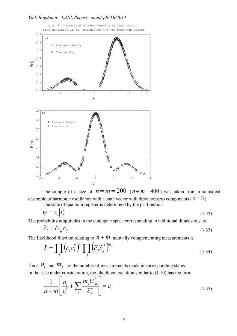
Yu.I. Bogdanov LANL Report quant-ph/0303014
9
Fig. 3. Comparison between density estimators and
true densities in (a) coordinate and (b) momentum spaces
x
P(x)
0,0
0,1
0,2
0,3
0,4
0,5
0,6
0,7
-3 -2 -1 0 1 2 3
Estimated density
True density
a)
p
P(p)
0,0
0,1
0,2
0,3
0,4
0,5
0,6
0,7
-3 -2 -1 0 1 2 3
Estimated density
True density
b)
The sample of a size of 200== mn ( 400=+mn ) was taken from a statisticalensemble of harmonic oscillators with a state vector with three nonzero components ( 3=s ).
The state of quantum register is determined by the psi function
ici=ψ (1.32)The probability amplitudes in the conjugate space corresponding to additional dimensions are
jiji cUc =~(1.33)
The likelihood function relating to mn + mutually complementing measurements is
( ) ( )∏ ∏=i j
mjj
nii
ji ccccL ** ~~(1.34)
Here, in and jm are the number of measurements made in corresponding states.In the case under consideration, the likelihood equation similar to (1.10) has the form
ij j
jij
i
i ccUm
cn
mn=
+
+ ∑ *
*
* ~1
(1.35)
Yu.I. Bogdanov LANL Report quant-ph/0303014
10
2. Constraint on the EnergyAs it has been already noted, the estimation of a state vector is associated with the problem
of suppressing high frequency terms in the Fourier series. In this section, we consider theregularization method based on the law of conservation of energy. Consider an ensemble ofharmonic oscillators (although formal expressions are written in general case). Taking into accountthe normalization condition without any constraints on the energy, the terms may appear that makea negligible contribution to the norm but arbitrary high contribution to the energy. In order tosuppress these terms, we propose to introduce both constraints on the norm and energy in themaximum likelihood method. The energy is readily estimated by the data of mutuallycomplementing experiments.
It is worth noting that in the case of potentials with a finite number of discrete levels inquantum mechanics [14], the problem of truncating the series does not arise (if solutions bounded atinfinity are considered).
We assume that the psi function is expanded in a series in terms of eigenfunctions of theenergy operator H (Hamiltonian):
( ) ( )∑−
=
=1
0
s
iii xcx ϕψ , (2.1)
where basis functions satisfy the equation
( ) ( )xExH iii ϕϕ =ˆ . (2.2)
Here, iE is the energy level corresponding to i -th state.
The mean energy corresponding to a statistical ensemble with a wave function ( )xψ is
( ) ( ) ∑∫−
=
∗∗ ==1
0
ˆs
iiii ccEdxxHxE ψψ . (2.3)
In arbitrary basis
∑−
=
∗=1
0
s
iijij ccHE , where ( ) ( )∫ ∗= dxxHxH jiij ϕϕ ˆ . (2.4)
Consider a problem of finding a maximum likelihood estimator of a state vector in view of aconstraint on the energy and norm of the state vector. In energy basis, the problem is reduced tomaximization of the following functional:
( ) ( )EccEccLS iiiii −−−−= ∗∗21 1ln λλ , (2.5)
where 1λ and 2λ are the Lagrange multipliers and Lln is given by (1.7).In this case, the likelihood equation has the form
( ) iijij cEcR 21 λλ += , (2.6)
where the R matrix is determined by (1.9).In arbitrary basis, the variational functional and the likelihood equation have the forms
( ) ( )EccHccLS ijijii −−−−= ∗∗21 1ln λλ , (2.7)
( ) ijijij ccHR 12 λλ =− . (2.8)
Having multiplied the both parts of (2.6) (or (2.8)) by ∗ic and summed over i , we obtain
the same result representing the relationship between the Lagrange multipliers:

Yu.I. Bogdanov LANL Report quant-ph/0303014
11
( ) Emn 21 λλ +=+ . (2.9)
The sample mean energy E (i.e., the sum of the mean potential energy that can bemeasured in the coordinate space and the mean kinetic energy measured in the momentum space)was used as the estimator of the mean energy in numerical simulations below.
Now, let us turn to the study of statistical fluctuations of a state vector in the problem underconsideration. We restrict our consideration to the energy representation in the case when theexpansion basis is formed by stationary energy states (that are assumed to be nondegenerate).
Additional condition (2.3) related to the conservation of energy results in the followingrelationship between the components
( )∑−
=
∗∗ =+=1
00
s
jjjjjjj ccEccEE δδδ . (2.10)
It turns out that both parts of the equality can be reduced to zero independently if oneassumes that a state vector to be estimated involves a time uncertainty, i.e., may differ from the trueone by a small time translation. The possibility of such a translation is related to the time-energyuncertainty relation.
The well-known expansion of the psi function in terms of stationary energy states, in viewof time dependence, has the form ( 1=h )
( ) ( )( ) ( )
( ) ( ) ( )∑
∑−=
=−−=
jjjjj
jjjj
xtiEtiEc
xttiEcx
ϕ
ϕψ
expexp
exp
0
0
(2.11)
In the case of estimating the state vector up to translation in time, the transformation
( )0exp tiEcc jjj =′ (2.12)
related to arbitrariness of zero-time reference 0t may be used to fit the estimated state vector to thetrue one.
The corresponding infinitesimal time translation leads us to the following variation of a statevector:
jjj cEitc 0=δ . (2.13)
Let cδ be any variation meeting both the normalization condition and the law of energyconservation. Then, from (1.15) and (2.3) it follows that
( ) 1εδ iccj
jj =∑ ∗, (2.14)
( ) 2εδ icEcj
jjj =∑ ∗, (2.15)
where 1ε and 2ε are arbitrary small real numbers.
In analogy with Sec.1, we divide the total variation cδ into unavoidable physical
fluctuation c2δ and variations caused by the gauge and time invariances:
jjjjj ccEitcic 20 δαδ ++= . (2.16)
Yu.I. Bogdanov LANL Report quant-ph/0303014
12
We will separate out the physical variation c2δ , so that it fulfills the conditions (2.14) and
(2.15) with a zero right part. It is possible if the transformation parameters α and 0t satisfy thefollowing set of linear equations:
=+
=+
202
10
εα
εα
tEE
tE. (2.17)
The determinant of (2.17) is the energy variance222 EEE −=σ . (2.18)
We assume that the energy variance is a positive number. Then, there exists a uniquesolution of the set (2.17). If the energy dissipation is equal to zero, the state vector has the onlynonzero component. In this case, the gauge transformation and time translation are dependent, sincethey are reduced to a simple phase shift.
In full analogy with the reasoning on the gauge invariance, one can show that in view ofboth the gauge invariance and time homogeneity, the transformation satisfying (2.17) providesminimization of the total variance of the variations (sum of squares of the components absolutevalues). Thus, one may infer that physical fluctuations are minimum possible fluctuationscompatible with the conservation of norm and energy.
Let us make an additional remark about the time translation introduced above. We willestimate the deviation between the estimated and exact state vectors by the difference between theirscalar product and unity. Then, one can state that the estimated state vector is closest to the true onespecified in the time instant that differs from the “true” one by a random quantity. In other words, aquantum ensemble can be considered as a time meter, statistical clock, measuring time within theaccuracy up to the statistical fluctuation asymptotically tending to zero with increasing number ofparticles of the system. Time measurement implies the comparison between the readings of real andreference systems. The dynamics of the state vector of a reference system corresponds to an infiniteensemble and is determined by the solution of the Schrödinger equation. The estimated state vectorof a real finite system is compared with the “world-line” of an ideal vector in the Hilbert space, andthe time instant when the ideal vector is closest to the real one is considered as the reading of thestatistical clock. Note that ordinary clock operates in the similar way: their readings correspond tothe situation when the scalar product of the real vector of a clock hand and the reference onemaking one complete revolution per hour reaches maximum value.
Assuming that the total variations are reduced to the physical ones, we assume hereafter that
( ) 0=∑ ∗
jjj ccδ , (2.19)
( ) 0=∑ ∗
jjjj cEcδ . (2.20)
The relationships found yield (in analogy with Sec.1) the conditions for the covariance
matrix ∗=Σ jiij ccδδ :
( ) 0=Σ∑j
jijc , (2.21)
( ) 0=Σ∑j
jjij cE . (2.22)
Consider the unitary matrix +U with the following two rows (zero and first):

Yu.I. Bogdanov LANL Report quant-ph/0303014
13
( ) ∗+ = jj cU 0 , (2.23)
( ) ( )1,...,1,0 1 −=
−=
∗+ sj
cEEU
E
jjj σ . (2.24)
This matrix determines the transition to principle components of the variation
ijij fcU δδ =+. (2.25)
According to (2.19) and (2.20), we have 010 == ff δδ identically in new variables so
that there remain only 2−s independent degrees of freedom.The inverse transformation is
cfU δδ = . (2.26)
On account of the fact that 010 == ff δδ , one may drop two columns (zero and first) in
the U matrix turning it into the factor loadings matrix L1,...,3,2 ;1,...,1,0 −=−== sjsicfL ijij δδ . (2.27)
The L matrix has s rows and 2−s columns. Therefore, it provides the transition from 2−sindependent variation principle components to s components of the initial variation.
In principal components, the Fisher information matrix and covariance matrix are given by
( ) ijf
ij mnI δ+= , (2.28)
( ) ijjifij mn
ff δδδ+
==Σ ∗ 1. (2.29)
In order to find the covariance matrix for the state vector components, we will take intoaccount the fact that the factor loadings matrix L differs form the unitary matrix U by theabsence of two aforementioned columns, and hence,
( )( ) ∗∗+ −−−−= ji
E
jijiijkjik cc
EEEEccLL 2σ
δ , (2.30)
mnLL
ffLLcc kjikrkjrikjiij +===Σ
+∗∗∗ δδδδ . (2.31)
Finally, the covariance matrix in the energy representation takes the form
( )( )( )
1,...,1,0,
112
−=
−−+−
+=Σ ∗
sji
EEEEcc
mn E
jijiijij σ
δ. (2.32)
It is easily verified that this matrix satisfies the conditions (2.21) and (2.22) resulting fromthe conservation of norm and energy.
The mean square fluctuation of the psi function is
( ) ( ) ( )mn
sTrccdxxcxcdx iijjii +−
=Σ=== ∗∗∗∗∫ ∫2
δδϕδϕδδψδψ . (2.33)
Yu.I. Bogdanov LANL Report quant-ph/0303014
14
The estimation of optimal number of harmonics in the Fourier series, similar to that in Sec.6of the Paper.1, has the form
( )1+ += ropt mnrfs , (2.34)
where the parameters r and f determine the asymptotics for the sum of squares of residuals:
( ) rsi
i sfcsQ ==∑
∞
=
2
. (2.35)
The norm existence implies only that 0>r . In the case of statistical ensemble of harmonicoscillators with existing energy, 1>r . If the energy variance is defined as well, 2>r .
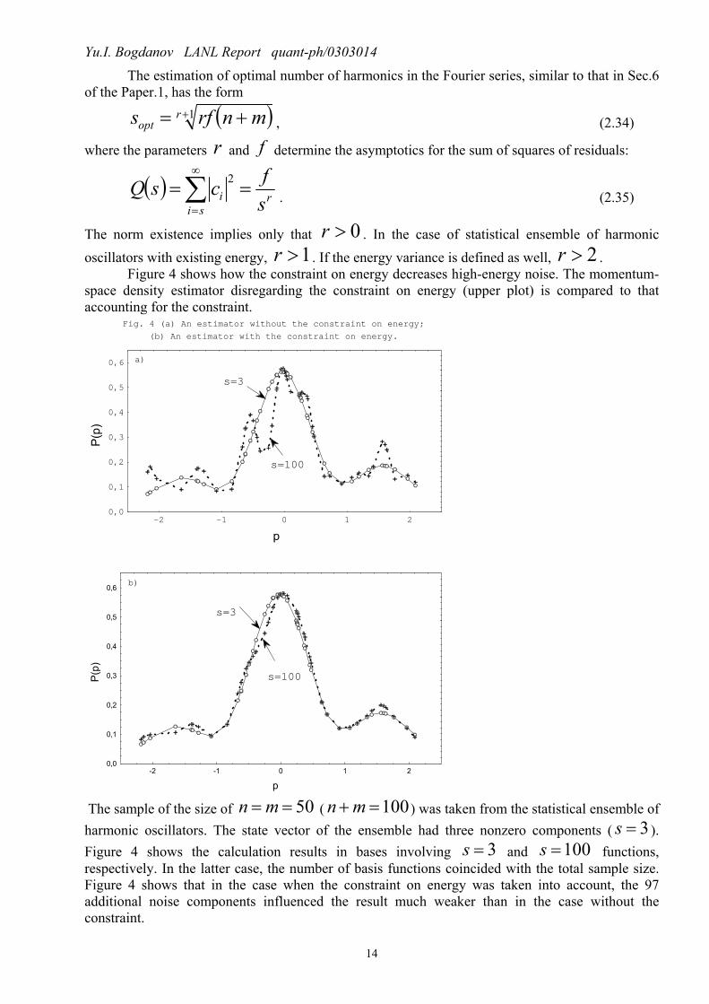
Figure 4 shows how the constraint on energy decreases high-energy noise. The momentum-space density estimator disregarding the constraint on energy (upper plot) is compared to thataccounting for the constraint.
Fig. 4 (a) An estimator without the constraint on energy;
(b) An estimator with the constraint on energy.
p
P(p)
0,0
0,1
0,2
0,3
0,4
0,5
0,6
-2 -1 0 1 2
s=3
s=100
a)
p
P(p)
0,0
0,1
0,2
0,3
0,4
0,5
0,6
-2 -1 0 1 2
s=3
s=100
b)
The sample of the size of 50== mn ( 100=+mn ) was taken from the statistical ensemble ofharmonic oscillators. The state vector of the ensemble had three nonzero components ( 3=s ).Figure 4 shows the calculation results in bases involving 3=s and 100=s functions,respectively. In the latter case, the number of basis functions coincided with the total sample size.Figure 4 shows that in the case when the constraint on energy was taken into account, the 97additional noise components influenced the result much weaker than in the case without theconstraint.
Yu.I. Bogdanov LANL Report quant-ph/0303014
15
3. Spin State Reconstruction
The aim of this section is to show the application of the approach developed above toreconstruct spin states (by an example of the ensemble of spin-1/2 particles).
We will look for the state vector in the spinor form
=
+
=
2
121 1
001
cc
ccψ (3.1)
The spin projection operator to direction nr
is
( ) ( )nsP nrr 1
212/1 σ±=±= (3.2)
We will set nr
by the spherical angles( ) ( )θϕθϕθ cos ,sinsin ,cossin,, == zyx nnnnr (3.3)
The probabilities for a particle to have positive and negative projections along the nrdirection are
( ) ( ) ψσψψψ nsPnP nrrr 1
212/1
21
+=+==+ (3.4)
( ) ( ) ψσψψψ nsPnP nrrr 1
212/1
21
−=−==− (3.5)
respectively.Direct calculation yields the following expressions for the probabilities under consideration:
( ) ( ) ( ) ( )[ ]2*21
*22
*11
*1 cos1 sin sincos1
21, ccccecceccPnP ii θθθθϕθ ϕϕ −++++== −
++r
(3.6)
( ) ( ) ( ) ( )[ ]2*21
*22
*11
*1 cos1 sin sincos1
21, ccccecceccPnP ii θθθθϕθ ϕϕ ++−−−== −
−−r
(3.7)
These probabilities evidently satisfy the condition( ) ( ) 1,, =+ −+ ϕθϕθ PP (3.8)
The likelihood function is given by the following product over all the directions involved inmeasurements:
( )( ) ( ) ( )( ) ( )nN
n
nN nPnPLr
r
r rr−+
−+∏= (3.9)
Here, ( )nN r+ and ( )nN r
− are the numbers of spins with positive and negative projections along
the nr direction. In order to reconstruct the state vector of a particle, one has to conductmeasurements at least in three noncomplanar (linearly independent) directions.The total number of measurements is
( ) ( ) ( )( )∑∑ −+ +==nn
nNnNnNNvv
rrr(3.10)
Yu.I. Bogdanov LANL Report quant-ph/0303014
16
In complete analogy to (1.8), we will find the likelihood equation represented by the set of two
equations in two unknown complex numbers 1c and 2c .
( )( )
( )[ ] ( )( )
( )[ ]∑ =
−−
+++ −
−
−−
+
+
n
ii
ccecnPnNcec
nPnN
N rr
r
r
r
12121
2sincos1
2sincos11 ϕϕ θθθθ
(3.11)
( )( )
( )[ ] ( )( )
( )[ ]∑ =
++−
+−+
−
−
+
+
n
ii
cccenPnNcce
nPnN
N rr
r
r
r
22121
2cos1sin
2cos1 sin 1 θθθθ ϕϕ
(3.12)
This system is nonlinear, since the probabilities ( )nP r+ and ( )nP r
− depend on the unknown
amplitudes 1c and 2c .This system can be easily solved by the method of iterations. The resultant estimated state
vector will differ from the true state vector by an asymptotically small random number (the squaredabsolute value of the scalar product of the true and estimated vectors is close to unity). Thecorresponding asymptotical formula has the form
( )
2~1
242
2
20 jjccN
χχ ==
− +
(3.13)
Here, 24 jχ is the random number with the chi-square distribution of j4 degrees of freedom,
and j is the particle spin ( 2/1=j in our case).
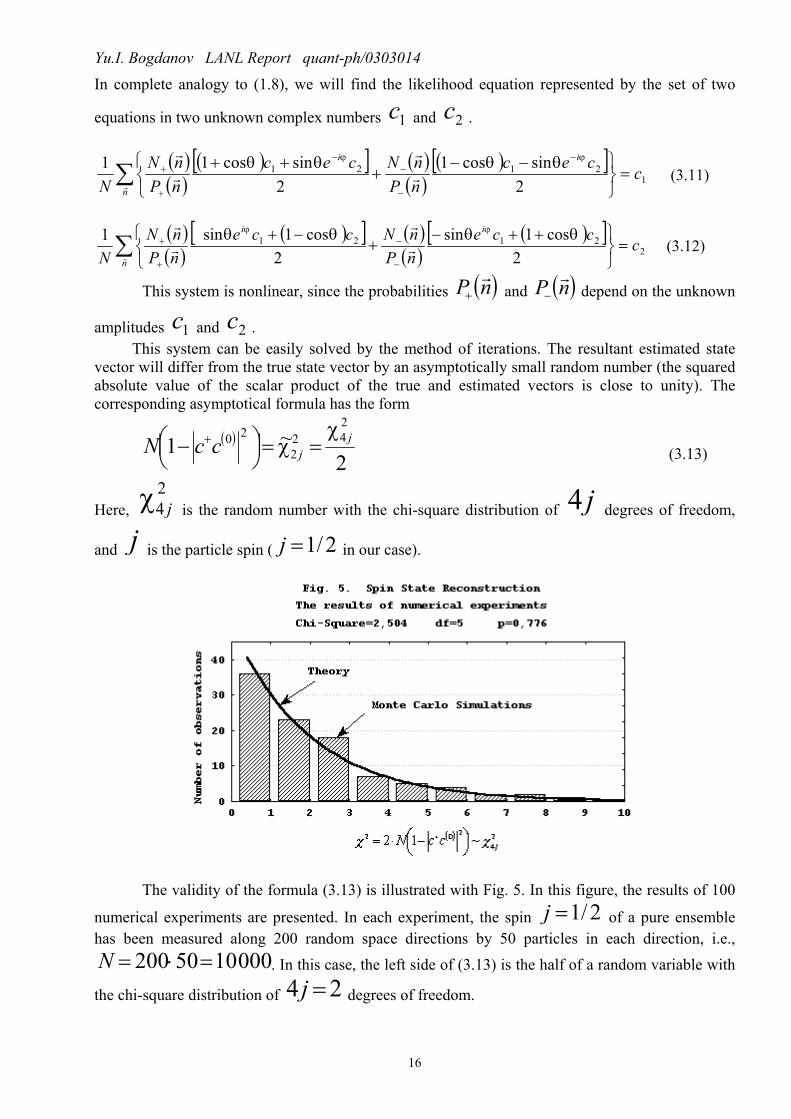
The validity of the formula (3.13) is illustrated with Fig. 5. In this figure, the results of 100
numerical experiments are presented. In each experiment, the spin 2/1=j of a pure ensemblehas been measured along 200 random space directions by 50 particles in each direction, i.e.,
000 1050200 =⋅=N . In this case, the left side of (3.13) is the half of a random variable with
the chi-square distribution of 24 =j degrees of freedom.

Yu.I. Bogdanov LANL Report quant-ph/0303014
17
Incoherent mixture is described in the framework of the density matrix. Two samples arereferred to as mutually incoherent if the squared absolute value of the scalar product of their statevector estimates is statistically significantly different from unity. The quantitative criterion is
( ) ( )
2~1
24,2
2,
221
21
21 jjcc
NNNN α
α
χχ =>
−
++
(3.14)
Here, 1N and 2N are the sample sizes, and 2
2, jαχ is the quantile corresponding to the
significance level α for the chi-square distribution of j2 degrees of freedom. The significance
level α describes the probability of error of the first kind, i.e., the probability to find samplesinhomogeneous while they are homogeneous (described by the same psi function).
Let us outline the process of reconstructing states with arbitrary spin. Let ( )jmψ be the
amplitude of the probability to have the projection m along the z axis in the initial coordinateframe (these are the quantities to be estimated by the results of measurements),
),...,1,( jjjm −−= . Let ( )jmψ
~ be the corresponding quantities in the rotated coordinate frame.
The probability to get the value m in measurement along the z′ axis is ( ) 2~ jmψ .
Both rotated and initial amplitudes are related to each other by the unitary transformation( ) ( ) ( )j
mj
mmj
m D ′′= ψψ *~(3.15)
The matrix ( )j
mmD ′ is a function of the Euler angles ( ) ( )γβα ,,j
mmD ′ , where the angles
α and β coincide with the spherical angles of the z′ axis with respect to the initial coordinate
frame xyz, so that ϕα = and θβ = . The angle γ corresponds to the additional rotation of
the coordinate frame with respect to the z′ axis (this rotation is insignificant in measuring the spin
projection along the z′ axis, and it can be set 0=γ ). The matrix ( )j
mmD ′ is described in detail in[14]. Note that our transformation matrix in (3.15) corresponds to the inverse transformation withrespect to that considered in [14].
The likelihood equation in this case has the form
( ) ( ) ( )( )
( )jm
mj
m
jmmm DN
Nψ
ψθϕθϕ
θϕ
=∑′ ′
′′
,,*~
,,1, (3.16)
where ( )θϕ,mN ′ is the number of spins with the projection m′ along the z′ axis with
direction determined by the spherical angles ϕ and θ , and N is the total number of measuredspins.
4. Mixture DivisionThere are two different methods for constructing the likelihood function for a mixture
resulting in two different ways to estimate the density (density matrix). In the first method (widely

Yu.I. Bogdanov LANL Report quant-ph/0303014
18
used in problems of estimating quantum states [7-10]), the likelihood function for the mixture isconstructed regardless a mixed (inhomogeneous) data structure (structureless approach). In thiscase, for the two-component mixture, we have
( ) ( )( )∏=
=n
ii ffccxpL
121
210 ,,, , (4.1)
where the mixture density is given by( ) ( ) ( )xpfxpfxp 2211 += ; (4.2)
( )xp1 and ( )xp2 are the densities of the mixture components; 1f and 2f , their weights.The normalization condition is
121 =+ ff (4.3)Here, it is assumed that all the points of the mixed sample ix ( ni ,...,2,1= ) are taken from
the same distribution ( ) ( ) ( )xpfxpfxp 2211 += . In other words, the mixture of twoinhomogeneous samples (i.e., taken from two different distributions) is treated as a homogeneoussample taken from an averaged distribution.
The second approach, which seems to be more physically adequate, is based on the notion ofa mixture as an inhomogeneous population (component approach). This implies that the mixedsample is considered as an inhomogeneous population with nfn 11 ≈ points taken from thedistribution with the density ( )xp1 and the other nfn 22 ≈ points, from the distribution with thedensity ( )xp2 .
This approach has also formal advantages compared to the first one: it provides higher valueof the likelihood function (and hence, higher value of information); besides that, basic theorystructures, such as the Fisher information matrix and covariance matrix, take a block form. Thus,the problem is reduced to the division of an inhomogeneous (mixed) population into homogeneous(pure) sub-populations.
In view of the mixed data structure, the likelihood function in the component approach isgiven by
( )( ) ( )( )∏∏+==
=n
nii
n
ii cxpcxpL
1
22
1
111
1
1
. (4.4)
Two different cases are possible:1- population is divided into components a priory from the physical considerations (for
instance, 1n values are taken from one source and 2n , from another source)2- dividing the population into components have to be done on the basis of data itself without
any information about sources (“blindly”)The first case does not present difficulties, since it is reduced to analyzing homogeneous
components in turn. The case when prior information about the sources is lacking requiresadditional considerations. In order to divide the mixture in this case, we will employ the so-calledrandomized (mixed) strategy. In this approach, we will consider the observation ix to be taken
from the first distribution with the probability ( )
( ) ( )ii
i
xpfxpfxpf
2211
11
+; and from the second one,
( )( ) ( )ii
i
xpfxpfxpf
2211
22
+. Having divided the sample into two population, we will find new estimates
of their weights by the formulas nnf 1
1 = and nnf 2
2 = , as well as estimates of the state vectors for
Yu.I. Bogdanov LANL Report quant-ph/0303014
19
each population (( )1c and
( )2c ) according to the algorithm presented above. Then, we will findthe component densities
( ) ( ) ( )211 xcxp ii ϕ= (4.5)
( ) ( ) ( )222 xcxp ii ϕ= (4.6)Finally, instead of the initial (prior) estimates of the weights and densities, we will find new
(posterior) weights and densities of the mixture components. Applying this (quasi- Bayesian)procedure repeatedly, we will arrive at a certain equilibrium state when the weights and densities ofthe components become approximately constant (more precisely, prior and posterior estimates ofweights and densities become indistinguishable within statistical fluctuations).
A random-number generator should be used for numerical implementation of the algorithmproposed. Each iteration starts with the setting of the random vector of the length n from ahomogeneous distribution on the segment [0,1]. If the same random vector is used at each iteration,the distribution of sample points between components will stop varying after some iterations, i.e.,each sample point will correspond to a certain mixture component (perhaps, up to insignificantinfinite looping, when a periodic exchange of a few points only happens). In this case, each randomvector corresponds to a certain random division of mixture into components that allows modelingthe fluctuation in a system.
Consider informational aspects of the problem of mixture division into components. Theresults presented below are based on the following mathematical inequality:
( ) ( )22112211222111 lnlnln pfpfpfpfppfppf ++≥+ , (4.7)that is valid if 121 =+ ff , and 1f , 2f , 1p , and 2p are arbitrary nonnegative numbers. We assume
also that 00ln0 = .Generally, the following inequality takes place
( ) ( ) ( )
≥ ∑∑∑
===
s
iii
s
iii
s
iiii pfpfppf
111lnln , (4.8)
if 11
=∑=
s
iif , and ( )sipf ii ,...,1 , = are arbitrary nonnegative numbers.
The equality sign in (4.8) takes place only in two cases: when either the probabilities are equal toeach other ( sppp === ...21 ) or one of the weights is equal to unity and the other weights are
zero ( 00 ,0 ,1 iiff ii ≠== ). In both cases, the mixed state is reduced to the pure one.
The logarithmic likelihood related to a certain observation ix in the case when we apply
the structureless approach and the functional 0L is evidently ( ) ( )( )ii xpfxpf 2211ln + .
In the component approach when we use the functional 1L and randomized (mixed) strategy, the
same observation corresponds to either the logarithmic likelihood ( )( )ixp1ln with the

Yu.I. Bogdanov LANL Report quant-ph/0303014
20
probability ( )
( ) ( )ii
i
xpfxpfxpf
2211
11
+ or the logarithmic likelihood ( )( )ixp2ln with the
probability ( )
( ) ( )ii
i
xpfxpfxpf
2211
22
+. In this case, the mean logarithmic likelihood is given by
( ) ( )( ) ( ) ( )( )
( ) ( )ii
iiii
xpfxpfxpxpfxpxpf
2211
222111 lnln++
This quantity turns out to be not smaller than the logarithmic likelihood in the first case( ) ( )( ) ( ) ( )( )
( ) ( ) ( ) ( )( )iiii
iiii xpfxpfxpfxpf
xpxpfxpxpf2211
2211
222111 lnlnln+≥
++
(4.9)
The validity of the last inequality at arbitrary values of the argument ix follows from the
inequality (4.7). Consider a continuous variable x instead of the discrete one ix and rewrite thelast inequality in the form
( ) ( )( ) ( ) ( )( )( ) ( )( ) ( ) ( )( )xpfxpfxpfxpf
xpxpfxpxpf
22112211
222111
lnlnln
++≥≥+
(4.10)
Integrating with respect to x , we find for the Boltzmann H function (representing theentropy with the opposite sign [15] )
0HHmix ≥ , (4.11)where
( ) ( )( ) ( )( ) ( ) ( )( )∫
∫++=
==
dxxpfxpfxpfxpf
dxxpxpH
22112211
0
ln
ln(4.12)
( ) ( ) ( ) ( )∫∫ += dxxpxpfdxxpxpfHmix 222111 lnln (4.13)
Thus, in the component approach, the Boltzmann H function is higher and the entropyHS −= is lower compared to the structureless description. This means that the representation
of data as a mixture of components results in more detailed (and hence, more informative)
description than that in the structureless approach. The difference 0HHI mixmix −= can beinterpreted as information produced in result of dividing the mixture into components. Thisinformation is lost in turning from the component description to structureless.
In general case of arbitrary number of mixture components, the mixture density is
( ) ( )∑=
=s
iii xpfxp
1, where 1
1=∑
=
s
iif (4.14)
From inequality (4.8), it follows that the component description generally corresponds to
higher (compared to that in the structureless description) value of the Boltzmann H function
0HHmix ≥ , (4.15)
where ( ) ( )∫= dxxpxpH ln0 (4.16)

Yu.I. Bogdanov LANL Report quant-ph/0303014
21
∑=
=s
iiimix HfH
1, ( ) ( )∫= dxxpxpH iii ln (4.17)
The information mixI produced in result of dividing the mixture into components belongs to therange
shmix SI ≤≤0 , (4.18)
where shS is the Shanon entropy [16] (the only difference is that we use e (instead of 2) as abase of logarithm)
( )∑=
−=s
iiish ffS
1ln (4.19)
The information mixI is equal to zero both in one-component mixture and when the componentsare indistinguishable (in this case, there is only one nonzero element in the diagonal representation
of the density matrix, i.e., it is a pure state). On the contrary, the information mixI reaches its
maximum ( shmix SI = ) when the densities of various components are separated from each other(their ranges of definition do not overlap).
Any density matrix may be represented in the form+=LLρ (4.20)
In the simplest case of second-order density matrix, the matrix L can be represented in theform of expansion
3322110 σσσ aaaEaL +++= , (4.21)
where E is an identity matrix of the second order and 321 ,, σσσ are the Pauli matrices.The expansion coefficients are given by
( )LTra21
0 = ( ) 3,2,1 21
== iLTra ii σ (4.22)
From the normalization condition ( ) 1=ρTr , it follows that
( ) 12 **00 =+ iiaaaa (4.23)
As is well known, the generators of the ( )2SU group are the spin matrices 2/σr . In the
general case of N -th order density matrix, the expansion similar to (4.21) have to involve the
generators of the ( )NSU group.The coordinate distribution density is
( ) ( ) ( ) ( ) ( ) ( ) ( )xxxxLLxxxP ijljilijij++ === ψψϕϕϕϕρ **
. (4.24)Here, we have introduced the “psi function” in the form of the row matrix
( ) ( ) ilil Lxx ϕψ = (4.25)
Yu.I. Bogdanov LANL Report quant-ph/0303014
22
or
( ) ( )Lxx Φ=ψ , (4.26)
where ( ) ( ) ( )( )xxx 10 ,ϕϕ=ΦThe expanded form of (4.26) is written as
( ) ( ) ( )( )( )( )( ) ( )( ) ( )( ) ( )( )xbxbxbxb
aEaxxx ii
14031201
010
,0,00,0,,
ϕϕϕϕσϕϕψ
+++==+=
(4.27)
where
301 aab += , 212 iaab += , 213 iaab −= , 304 aab −= (4.28)Similarly, the momentum distribution density is
( ) ( ) ( )pppP += ψψ ~~~, (4.29)
where
( ) ( ) ( )( )( )( )( ) ( )( ) ( )( ) ( )( )pbpbpbpb
aEappp ii
14031201
010~,0~,00,~0,~
~,~~
ϕϕϕϕσϕϕψ
+++==+=
(4.30)
Here, ( ) ( )pp 10~ ,~ ϕϕ are the Fourier transforms of the functions ( ) ( )xx 10 , ϕϕ .
The expansions (4.27) and (4.30) show that the reconstruction method that is not based onthe prior information about the mixture sources does not allow one to divide the estimates of the
parameters 1b and 3b , as well as those of 2b и 4b . On the contrary, if the estimation method is apriory based on the fact that several observations correspond to the first source, and the other, to the
second; we can use the coefficients 1b and 2b to estimate the parameters of the first component,
and 3b and 4b , for the second one. The problem of estimating the mixture parameters is reduced toreconstructing pure states.
In this paper, major attention is paid to estimating the pure states representing a morefundamental object compared to mixed states. The measurement results together with classicalinformation about either the sources of particles or the environment allow one (in principle) toreduce the study of the density matrix to the study of mixture components representing pure states.It is necessary to keep in mind that dividing mixture into components is not unique. However, theresultant density matrix is the same for any expansion within the statistical fluctuations.
The results that we have found for the second-order density matrices are evidently valid ingeneral case.
In the case when classical information on the sources of particles is partially or totallyunavailable, it is purposeful to use quasi- Bayesian algorithm proposed above to divide mixture intocomponents.
The mean trace of the squared deviation between the estimated and true density matrices is(if the division into components is a priory known)
( )( ) ( )NsTr 1220 −
=−ρρ , (4.31)

Yu.I. Bogdanov LANL Report quant-ph/0303014
23
where N is the total sample size and s , the dimension of Hilbert space.If the mixture has to be divided “blindly”, the accuracy of estimation somewhat decreases
due to fluctuations in the component weights.
5. Root estimator and quantum dynamics: statistical root quantizationLet the dynamics of a classical particle be determined by the Hamilton equation
pm
xdtd rr 1
= (5.1)
xUp
dtd
rr
∂∂
−= (5.2)
Assume that the mechanical equations are satisfied only for statistically averaged quantities
pm
xdtd rr 1
= (5.3)
xUp
dtd
rr
∂∂
−= , (5.4)
where the averaged values result from introducing distributions
( )∫= dxxxPx rr(5.5)
( )∫= dpppPp rr ~(5.6)
( )∫ ∂∂
=∂∂ dx
xUxP
xU
rr (5.7)
In the expanded form, these averaged equations are evidently written as
( )( ) ( )( )∫∫ = dpppPm
dxxxPdtd rr ~1
(5.8)
( )( ) ( )
∂∂
−= ∫∫ dxxUxPdpppP
dtd
rr~
(5.9)
Differentiating (5.8) in view of (5.9), we find the averaged Newton's second law of motion
( )( ) ( )
∂∂
−= ∫∫ dxxUxP
mdxxxP
dtd
rr 1
2
2
(5.10)

Yu.I. Bogdanov LANL Report quant-ph/0303014
24
Let us require the density ( )xP to admit the root expansion, i.e.,
( ) ( )2xxP ψ= , (5.11)where
( ) ( ) ( )xtcx jj ϕψ = (5.12)We will search for the time dependence of the expansion coefficients in the form of harmonicdependence
( ) ( )tictc jjj ω−= exp0 . (5.13)Then, Eq. (5.10) yields
( ) ( )( )( )( )tij
xUkcc
tijxkccm
kjkj
kjkjkj
ωω
ωωωω
−−∂∂
=
=−−−
exp
exp
*00
*00
2
r
r
(5.14)
Here, the summation over recurring indices j and k is meant. The matrix elements in (5.14) aredetermined by the formulas
( ) ( )dxxxxjxk jk ϕϕ *∫=rr
(5.15)
( ) ( )dxxxUxj
xUk jk ϕϕ *∫ ∂
∂=
∂∂
rr (5.16)
In order for the expression (5.14) to be satisfied at any instant of time for arbitrary initialamplitudes, the left and right sides are necessary to be equal for each matrix element. Therefore,
( ) jxUkjxkm kj r
r
∂∂
=− 2ωω(5.17)
This expression is a matrix equation of the Heisenberg quantum dynamics in the energyrepresentation (written in the form similar to that of the Newton's second law of motion). The basisfunctions and frequencies satisfying (5.17) are the stationary states and frequencies of a quantumsystem, respectively (in accordance with the equivalence of the Heisenberg and Schrödingerpictures).
Indeed, let us construct the diagonal matrix from the system frequencies jω . The matrix underconsideration is Hermitian, since the frequencies are real numbers. This matrix is the representation
of a Hermitian operator with eigenvalues jω, i.e.,
jjH jωh= (5.18)Let us find an explicit form of this operator. In view of (5.18), the matrix relationship (5.17) can berepresented in the form of the operator equation
[ ][ ] Um
xHH ∂= ˆ2hr
, (5.19)

Yu.I. Bogdanov LANL Report quant-ph/0303014
25
where xr∂∂
=∂ is the operator of differentiation and [ ] , the commutator.
The Hamiltonian of a system
( )xUm
H +∂−= 22
ˆ2h
(5.20)
is the solution of operator equation (5.19).
Thus, if the root density estimator is required to satisfy the averaged classical equations ofmotion, the basis functions and frequencies of the root expansion cannot be arbitrary, but have to beeigenfunctions and eigenvalues of the system Hamiltonian, respectively.
The relationships providing that the averaged equations of classical mechanics are satisfiedfor quantum systems are referred to as the Ehrenfest equations [in our case, Eqs. (5.8) and (5.9)].These equations are insufficient to describe quantum dynamics. As it has been shown above, anadditional condition allowing one to transform a classical system into the quantum one (i.e.,quantization condition) is actually the requirement for the density to be of the root form.
Thus, if we wish to turn from the rigidly deterministic (Newtonian) description of adynamical system to the statistical one, it is natural to use the root expansion of the densitydistribution to be found, since only in this case a stable statistical model can be found. On the otherhand, the choice of the root expansion basis determined by the eigenfunctions of the energyoperator (Hamiltonian) is not simply natural, but the only possible way consistent with thedynamical laws.
ConclusionsLet us state a short summary.The root state estimator may be applied to analyze the results of experiments with micro
objects as a natural instrument to solve the inverse problem of quantum mechanics: estimation ofpsi function by the results of mutually complementing (according to Bohr) experiments.Generalization of the maximum likelihood principle to the case of statistical analysis of mutuallycomplementing experiments is proposed.
The Fisher information matrix and covariance matrix are considered for a quantumstatistical ensemble. It is shown that the constraints on the norm and energy are related to the gaugeand time translation invariances. The constraint on the energy is shown to result in the suppressionof high-frequency noise in a state vector approximated.
It is shown that the spin wave function can be estimated by the method similar to that usedto estimate the coordinate psi function.
It is purposeful to solve the problem of reconstructing the mixed state described by thedensity matrix by dividing the initial data into homogeneous components. In the case when the priorinformation is lacking, one should use the self-consistent quasi- Bayesian algorithm proposed inthis paper.
It is shown that the requirement for the density to be of the root form is the quantizationcondition. Actually, one may say about the root principle in statistical description of dynamicsystems. According to this principle, one has to perform the root expansion of the distributiondensity in order to provide the stability of statistical description. On the other hand, the rootexpansion is consistent with the averaged laws of classical mechanics when the eigenfunctions ofthe energy operator (Hamiltonian) are used as basis functions. Figuratively speaking, there is no aregular statistical method besides the root one, and there is no regular statistical mechanics besidesthe quantum one.

Yu.I. Bogdanov LANL Report quant-ph/0303014
26
References1. U. Fano Description of States in Quantum Mechanics by Density Matrix and Operator
Techniques// Rev. Mod. Phys. 1957. V. 29. P.74.2. R. G. Newton und B. Young Measurability of the Spin Density Matrix //Ann. Phys. 1968. V.49.
P.393.3. A. Royer Measurement of the Wigner Function //Phys. Rev. Lett. 1985. V.55. P.2745.4. G. M. D’Ariano, M. G. A. Paris and M. F. Sacchi Quantum tomography // LANL Report quant-
ph/0302028. 2003. 102p5. K. Vogel und H. Risken Determination of quasiprobability distributions in terms of probability
distributions for the rotated quadrature phase// Phys. Rev. A. 1989. V.40. P.2847.6. T. Opatrny, D.-G. Welsch and W. Vogel Least-squares inversion for density-matrix
reconstruction // LANL Report quant-ph/9703026. 1997. 16p.7. Z. Hradil Quantum state estimation // Phys. Rev. A. 1997. V. 55. 1561 (R)8. K. Banaszek Maximum-likelihood estimation of photon-number distribution from homodyne
statistics // Phys. Rev. A 1998. V.57. P.5013-50159. K. Banaszek, G. M. D’Ariano, M. G. A. Paris, and M. F. Sacchi Maximum-likelihood
estimation of the density matrix // Phys. Rev. A. 2000. V. 61. 010304 (R).10. G. M. D’Ariano, M. G. A. Paris and M. F. Sacchi Parameters estimation in quantum optics//
Phys. Rev. A 2000. V.62. 02381511. N. Bohr Collected works. Amsterdam. North-Holland Pub. Co. 1972-1987. v.1-10. v.6
Foundations of quantum physics I. (1926-1932).12. M.B.Mensky, Quantum measurements and decoherence. Kluwer. Dordrecht. 2000 (Russian
translation: Fizmatlit, Moscow, 2001).13. A. N. Tikhonov and V. A. Arsenin. Solutions of ill-posed problems. W.H. Winston. Washington
D.C. 197714. L. D. Landau and E. M. Lifschitz Quantum Mechanics (Non-Relativistic Theory). 3rd ed.
Pergamon Press. Oxford. 1991.15. E. M. Lifschitz and L. P. Pitaevski Physical kinetics. Oxford- 2. ed. Pergamon Press. 1981.
(Landau-Lifschitz. Course of theoretical physics. V.10)16. C.E. Shannon and W. Weaver The Mathematical Theory of Communication. University of
Illinois Press. New York. 1949.17. P. Ehrenfest Bemerkung über die angenaherte Gültigkeit der klassischen Mechanik innerhalb
der Quanten Mechanik // Z. Phys. 1927. 45. S. 455-457. (English translation: P. EhrenfestCollected Scientific Papers. Amsterdam. 1959. P.556-558).