YU Xiangyuyuxy@scut.edu.cn

2016/10/14

Frequency and Spectrum Types of Waves Propagation Model Free-Space Propagation Path Loss Fading: Slow Fading / Fast Fading Doppler Shift Delay Spread

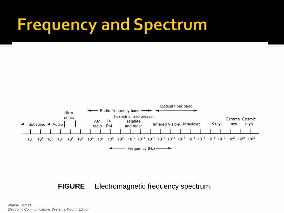
FIGURE Electromagnetic frequency spectrum.

Wayne Tomasi

Electronic Communications Systems, Fourth Edition

Tomasi

Advanced Electronic Communications

Systems, 6e

FIGURE Electromagnetic wavelength

spectrum

Frequency and wave length

= c/f

wave length , speed of light c 3x108m/s, frequency f

1 Mm

300

Hz

10 km

30 kHz

100 m

3 MHz

1 m

300 MHz

10 mm

30 GHz

100

m

3 THz

1 m

300

THz

visible

light

VL

F

LF M

F

HF VHF UHF SHF EHF infrared UV

optical transmissioncoax cabletwisted

pair

Schiller P26

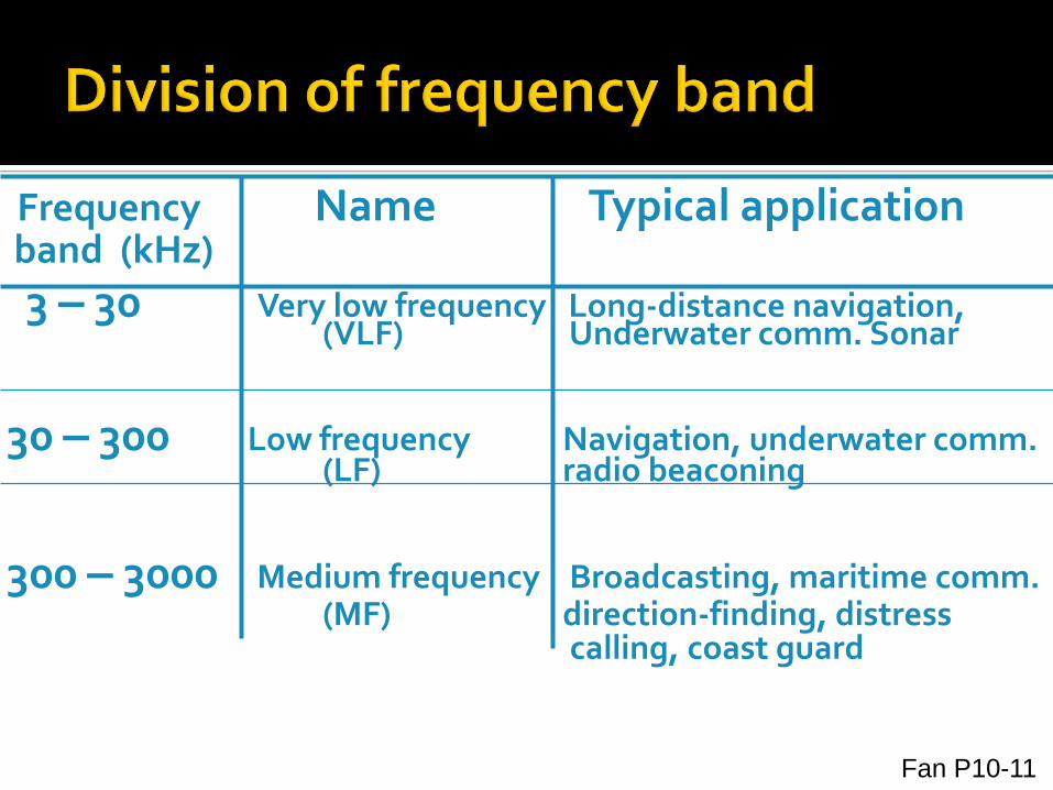
Frequency Name Typical applicationband (kHz)

3 – 30 Very low frequency Long-distance navigation, (VLF) Underwater comm. Sonar

30 – 300 Low frequency Navigation, underwater comm.(LF) radio beaconing

300 – 3000 Medium frequency Broadcasting, maritime comm.(MF) direction-finding, distress

calling, coast guard

Fan P10-11

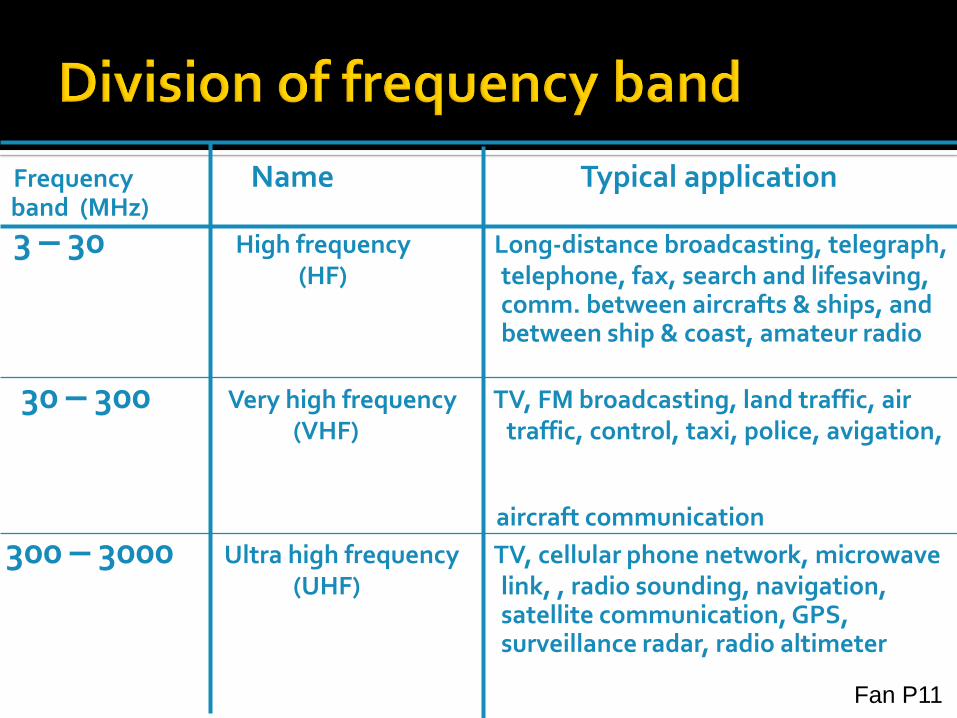
Frequency Name Typical applicationband (MHz)

3 – 30 High frequency Long-distance broadcasting, telegraph,(HF) telephone, fax, search and lifesaving,

comm. between aircrafts & ships, andbetween ship & coast, amateur radio

30 – 300 Very high frequency TV, FM broadcasting, land traffic, air(VHF) traffic, control, taxi, police, avigation,

aircraft communication

300 – 3000 Ultra high frequency TV, cellular phone network, microwave (UHF) link, , radio sounding, navigation,

satellite communication, GPS, surveillance radar, radio altimeter

Fan P11

Frequency Name Typical applicationband (GHz)

3 – 30 Super high frequency Satellite comm., radio altimeter,(SHF) microwave link, aircraft radar,

meteorological radar, publicland vehicle communication

30 – 300 Extremely high Radar landing system, satellitefrequency (EHF) comm., vehicle comm., railway

traffic

300 – 3000 Submillimeter wave Experiment, not designated

（0.1 – 1 mm） Fan P11

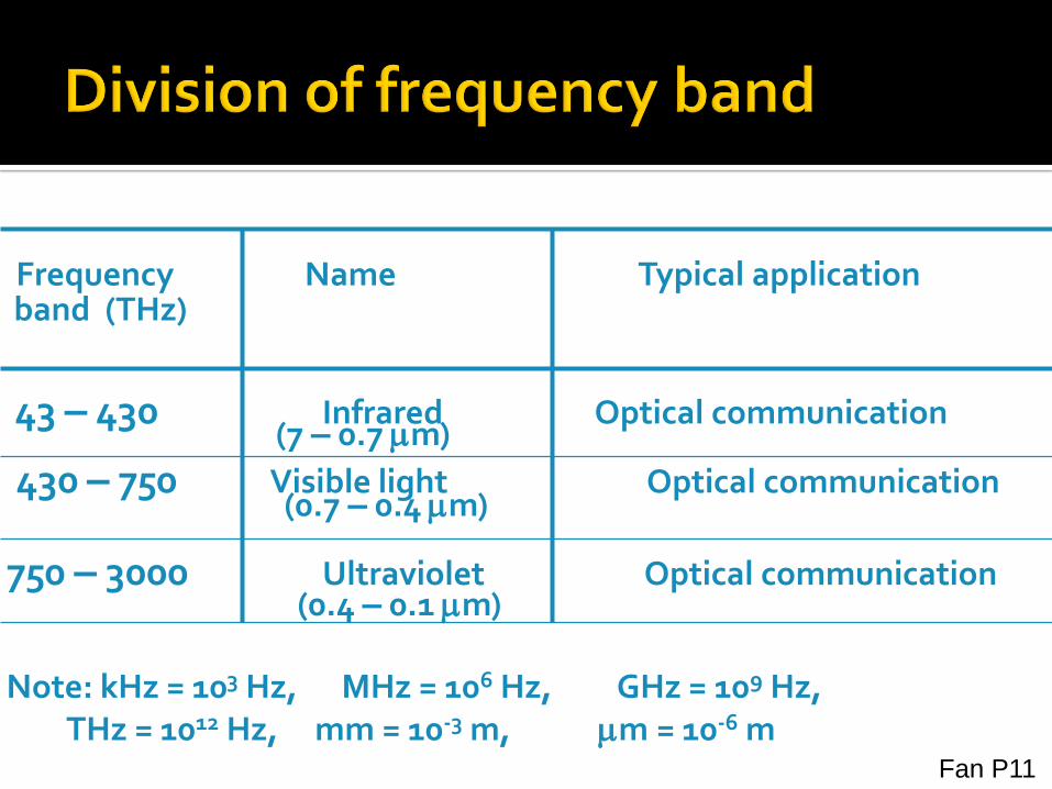
Frequency Name Typical applicationband (THz)

43 – 430 Infrared Optical communication(7 – 0.7 m)

430 – 750 Visible light Optical communication(0.7 – 0.4 m)

750 – 3000 Ultraviolet Optical communication (0.4 – 0.1 m)

Note: kHz = 103 Hz, MHz = 106 Hz, GHz = 109 Hz, THz = 1012 Hz, mm = 10-3 m, m = 10-6 m

Fan P11

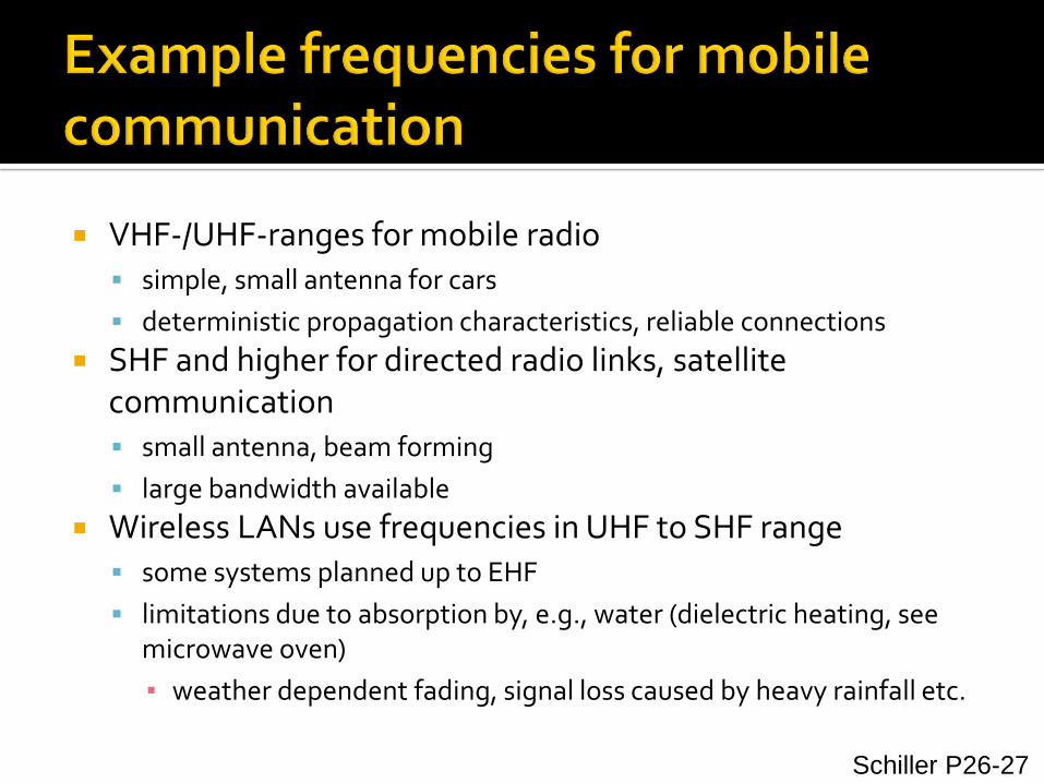
VHF-/UHF-ranges for mobile radio simple, small antenna for cars

deterministic propagation characteristics, reliable connections

SHF and higher for directed radio links, satellite communication small antenna, beam forming

large bandwidth available

Wireless LANs use frequencies in UHF to SHF range some systems planned up to EHF

limitations due to absorption by, e.g., water (dielectric heating, see microwave oven)

▪ weather dependent fading, signal loss caused by heavy rainfall etc.

Schiller P26-27

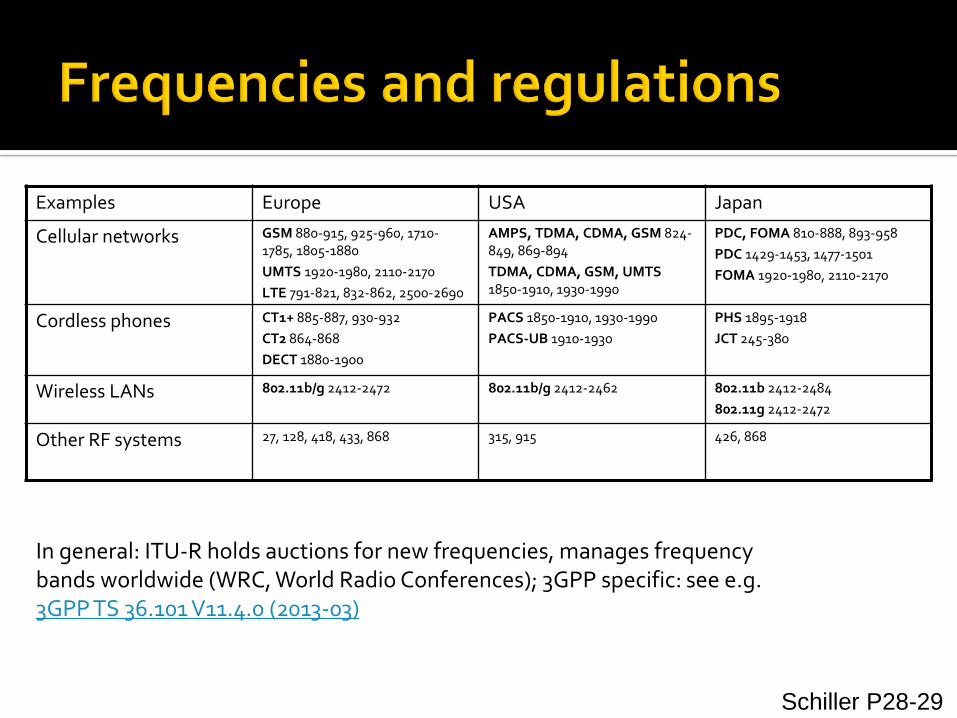
Examples Europe USA Japan

Cellular networks GSM 880-915, 925-960, 1710-1785, 1805-1880

UMTS 1920-1980, 2110-2170

LTE 791-821, 832-862, 2500-2690

AMPS, TDMA, CDMA, GSM 824-849, 869-894

TDMA, CDMA, GSM, UMTS1850-1910, 1930-1990

PDC, FOMA 810-888, 893-958

PDC 1429-1453, 1477-1501

FOMA 1920-1980, 2110-2170

Cordless phones CT1+ 885-887, 930-932

CT2 864-868

DECT 1880-1900

PACS 1850-1910, 1930-1990

PACS-UB 1910-1930

PHS 1895-1918

JCT 245-380

Wireless LANs 802.11b/g 2412-2472 802.11b/g 2412-2462 802.11b 2412-2484

802.11g 2412-2472

Other RF systems 27, 128, 418, 433, 868 315, 915 426, 868

In general: ITU-R holds auctions for new frequencies, manages frequency bands worldwide (WRC, World Radio Conferences); 3GPP specific: see e.g. 3GPP TS 36.101 V11.4.0 (2013-03)

Schiller P28-29

Tomasi

Advanced Electronic Communications

Systems, 6e

TABLE Microwave Radio-Frequency Assignments

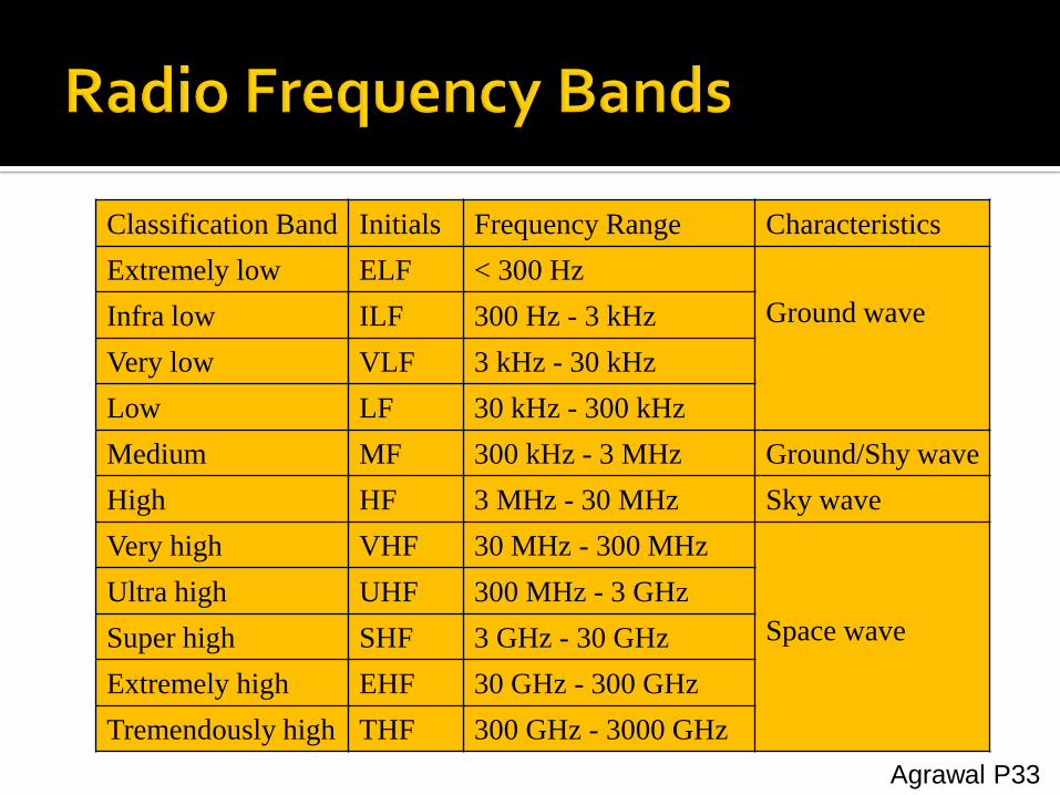
Classification Band Initials Frequency Range Characteristics

Extremely low ELF < 300 Hz

Ground waveInfra low ILF 300 Hz - 3 kHz

Very low VLF 3 kHz - 30 kHz

Low LF 30 kHz - 300 kHz

Medium MF 300 kHz - 3 MHz Ground/Shy wave

High HF 3 MHz - 30 MHz Sky wave

Very high VHF 30 MHz - 300 MHz

Space wave

Ultra high UHF 300 MHz - 3 GHz

Super high SHF 3 GHz - 30 GHz

Extremely high EHF 30 GHz - 300 GHz

Tremendously high THF 300 GHz - 3000 GHz

Agrawal P33

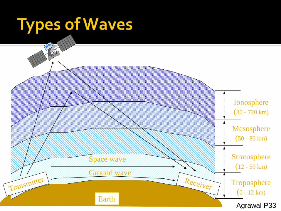
Earth

Ground wave

Space wave

Ionosphere

(80 - 720 km)

Mesosphere

(50 - 80 km)

Stratosphere

(12 - 50 km)

Troposphere

(0 - 12 km)

Agrawal P33

Ground-wave propagation Sky-wave propagation Line-of-sight propagation

Stallings P101

Figure Propagation of radio frequencies.

Couch P41

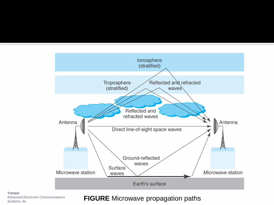
Tomasi

Advanced Electronic Communications

Systems, 6eFIGURE Microwave propagation paths

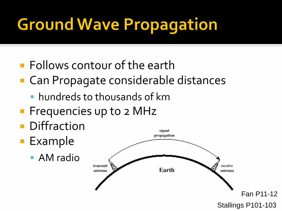
Follows contour of the earth Can Propagate considerable distances

hundreds to thousands of km

Frequencies up to 2 MHz Diffraction Example

AM radio

Stallings P101-103

Fan P11-12

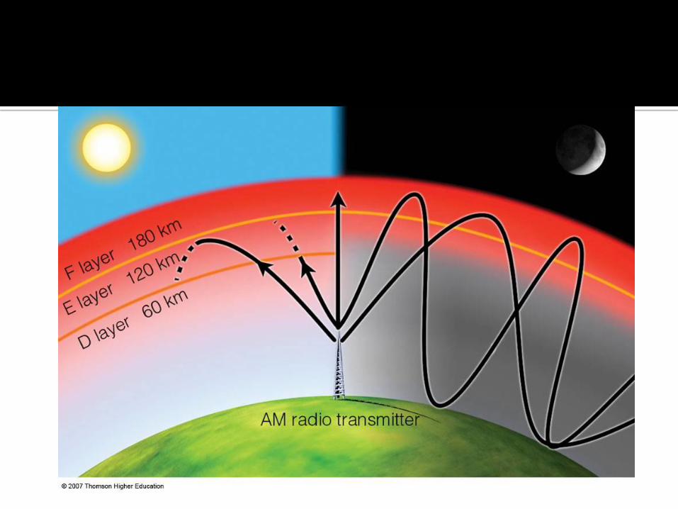
Signal reflected from ionized layer of atmosphere back down to earth

Signal can travel a number of hops, back and forth between ionosphere(60 ~ 400 km) and earth’s surface

One hop max. propagation distance：4000 km Propagation distance by multi-hops: >10000 km Reflection effect caused by refraction Frequency：2 ~ 30 MHz Examples

Amateur radio

CB(Citizens Band) radio

Stallings P101-103

Wayne Tomasi

Electronic Communications Systems, Fourth Edition

FIGURE Critical angle

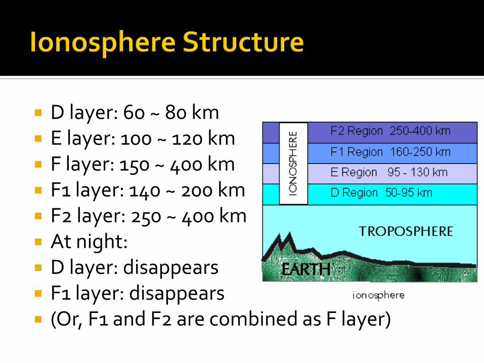
D layer: 60 ~ 80 km E layer: 100 ~ 120 km F layer: 150 ~ 400 km F1 layer: 140 ~ 200 km F2 layer: 250 ~ 400 km At night: D layer: disappears F1 layer: disappears (Or, F1 and F2 are combined as F layer)

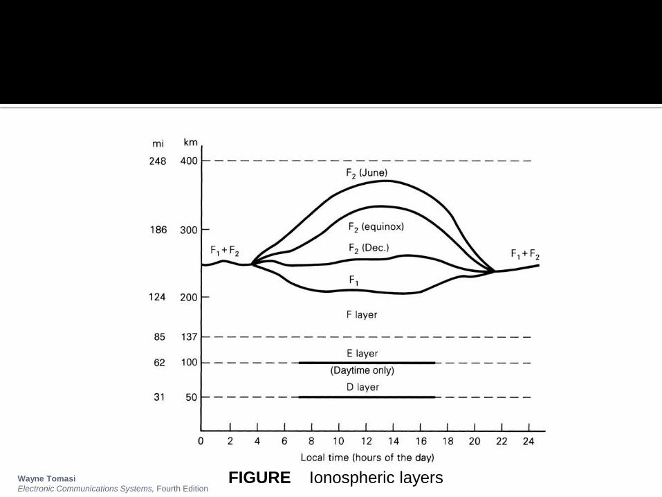
Wayne Tomasi

Electronic Communications Systems, Fourth EditionFIGURE Ionospheric layers

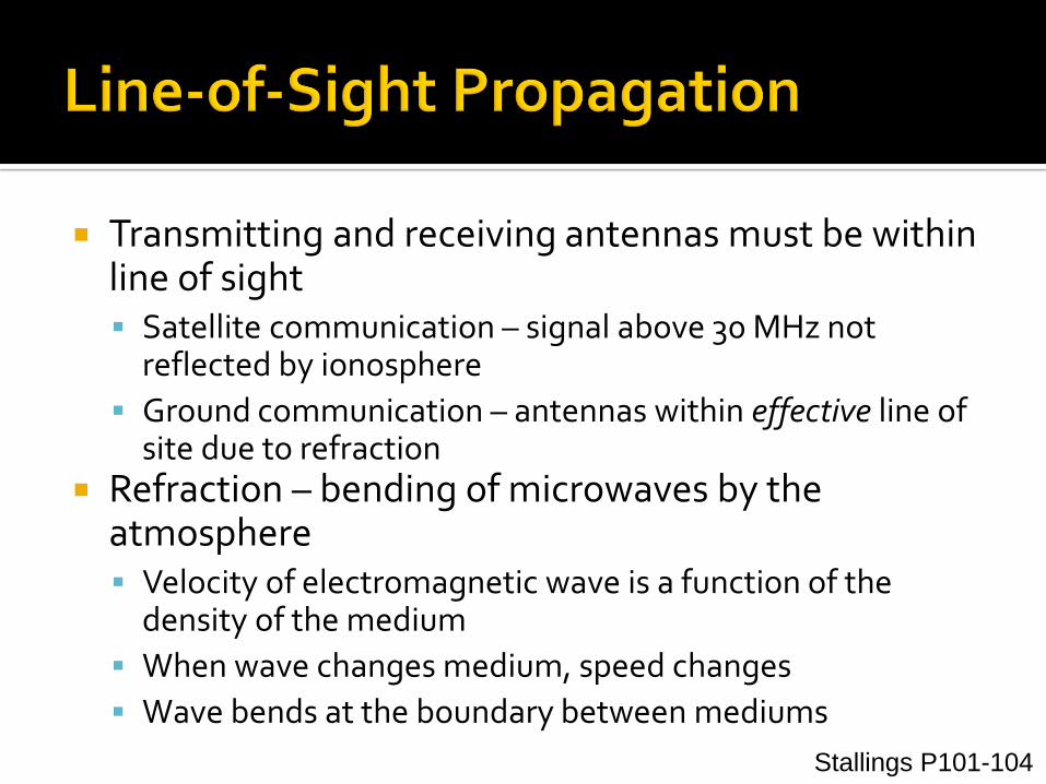
Transmitting and receiving antennas must be within line of sight Satellite communication – signal above 30 MHz not

reflected by ionosphere

Ground communication – antennas within effective line of site due to refraction

Refraction – bending of microwaves by the atmosphere Velocity of electromagnetic wave is a function of the

density of the medium

When wave changes medium, speed changes

Wave bends at the boundary between mediums

Stallings P101-104

Couch P43

2 2 2

2 2

( )

2

d r r h

d rh h

2 2 2d h rh rh

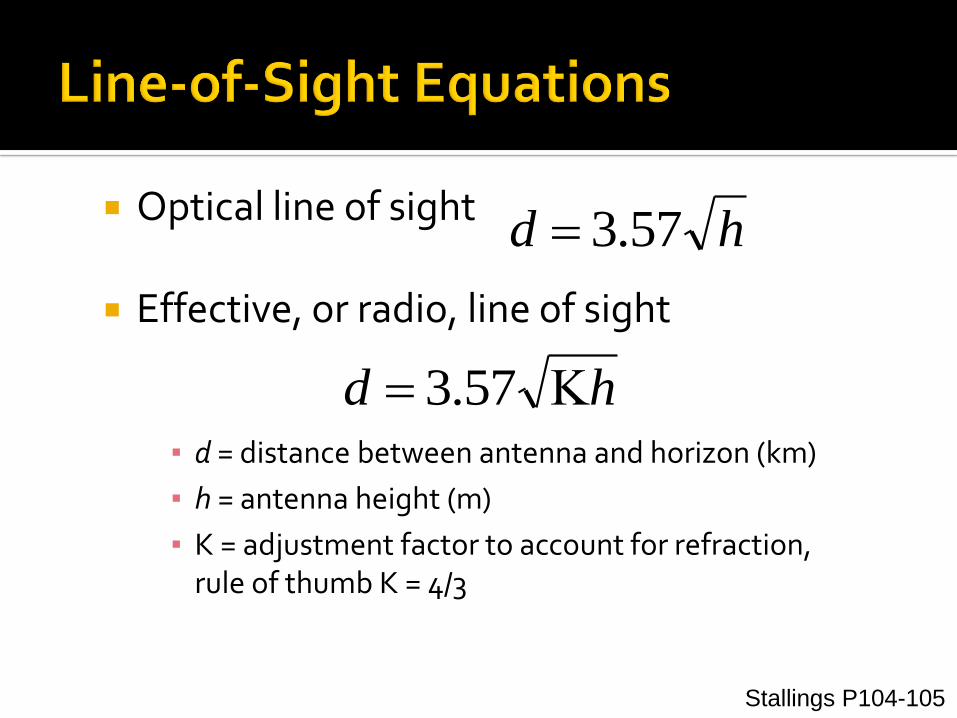
Optical line of sight

Effective, or radio, line of sight

▪ d = distance between antenna and horizon (km)

▪ h = antenna height (m)

▪ K = adjustment factor to account for refraction, rule of thumb K = 4/3

hd 57.3

hd 57.3

Stallings P104-105

FIGURE Space waves and radio horizon

Wayne Tomasi

Electronic Communications Systems, Fourth Edition Stallings P103

Maximum distance between two antennas for LOS propagation:

▪ h1 = height of antenna one

▪ h2 = height of antenna two

2157.3 hh

Stallings P105

My result : 101km

Tomasi

Advanced Electronic Communications

Systems, 6e

FIGURE Microwave radio communications link

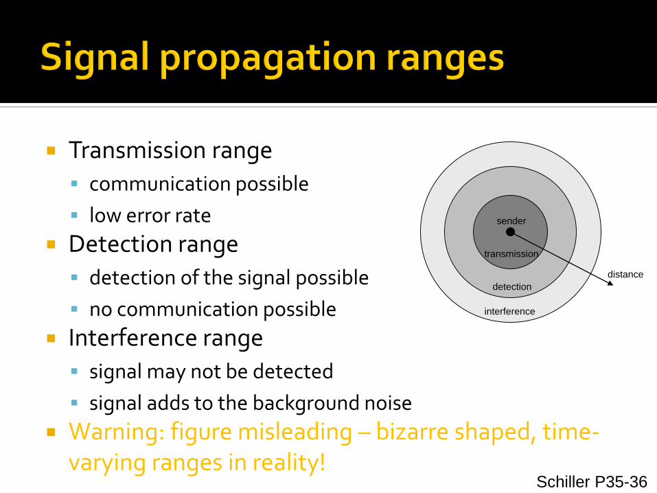
Transmission range

communication possible

low error rate

Detection range

detection of the signal possible

no communication possible

Interference range

signal may not be detected

signal adds to the background noise

Warning: figure misleading – bizarre shaped, time-varying ranges in reality!

distance

sender

transmission

detection

interference

Schiller P35-36

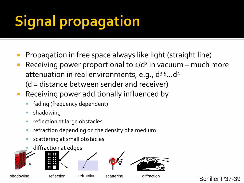
Propagation in free space always like light (straight line) Receiving power proportional to 1/d² in vacuum – much more

attenuation in real environments, e.g., d3.5…d4

(d = distance between sender and receiver) Receiving power additionally influenced by

fading (frequency dependent)

shadowing

reflection at large obstacles

refraction depending on the density of a medium

scattering at small obstacles

diffraction at edges

reflection scattering diffractionshadowing refractionSchiller P37-39

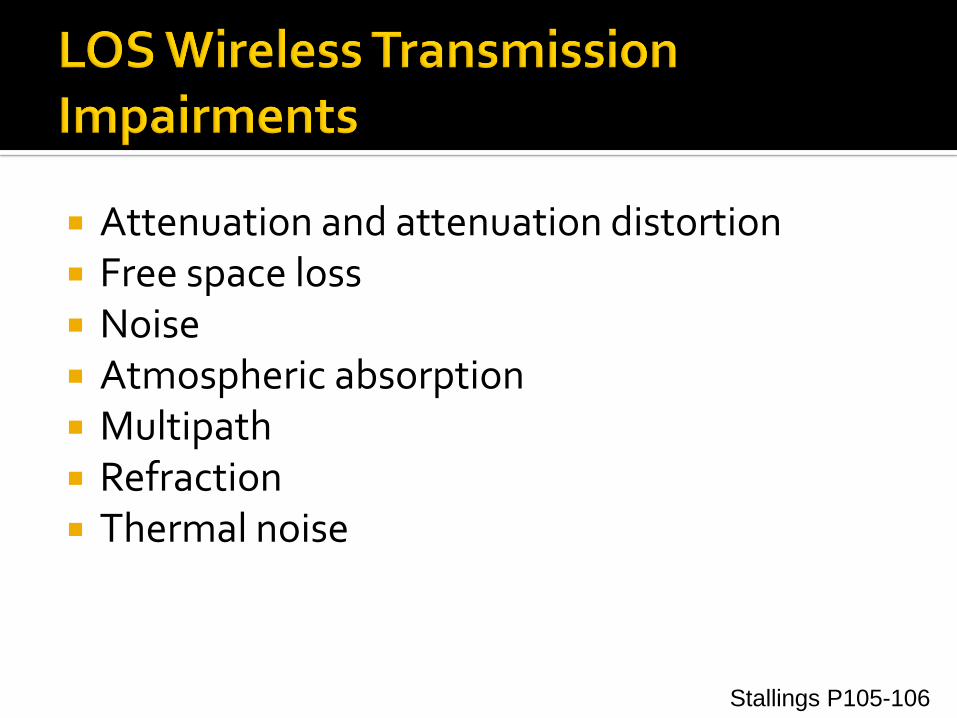
Attenuation and attenuation distortion Free space loss Noise Atmospheric absorption Multipath Refraction Thermal noise

Stallings P105-106

Strength of signal falls off with distance over transmission medium

Attenuation factors for unguided media:

Received signal must have sufficient strength so that circuitry in the receiver can interpret the signal

Signal must maintain a level sufficiently higher than noise to be received without error

Attenuation is greater at higher frequencies, causing distortion

Stallings P106

Atten

uatio

n(d

B/k

m)

Vapor

Oxygen

Frequency (GHz)(a) Attenuation of oxygen & vapor（concentration 7.5 g/m3）

Atten

uatio

n(d

B/k

m)

Rainfall rate

Frequency (GHz)(b) Attenuation of rainfall Fan P14

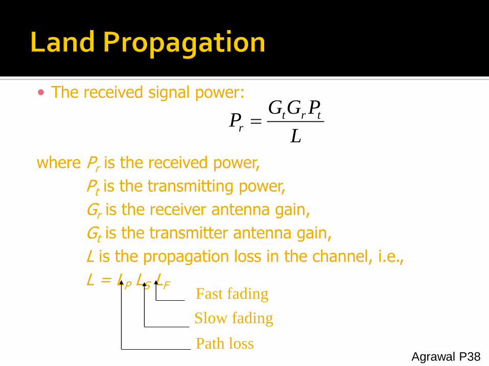
The received signal power:

where Pr is the received power,

Pt is the transmitting power,

Gr is the receiver antenna gain,

Gt is the transmitter antenna gain,

L is the propagation loss in the channel, i.e.,

L = LP LS LF

L

PGGP trt

r

Fast fading

Slow fading

Path lossAgrawal P38

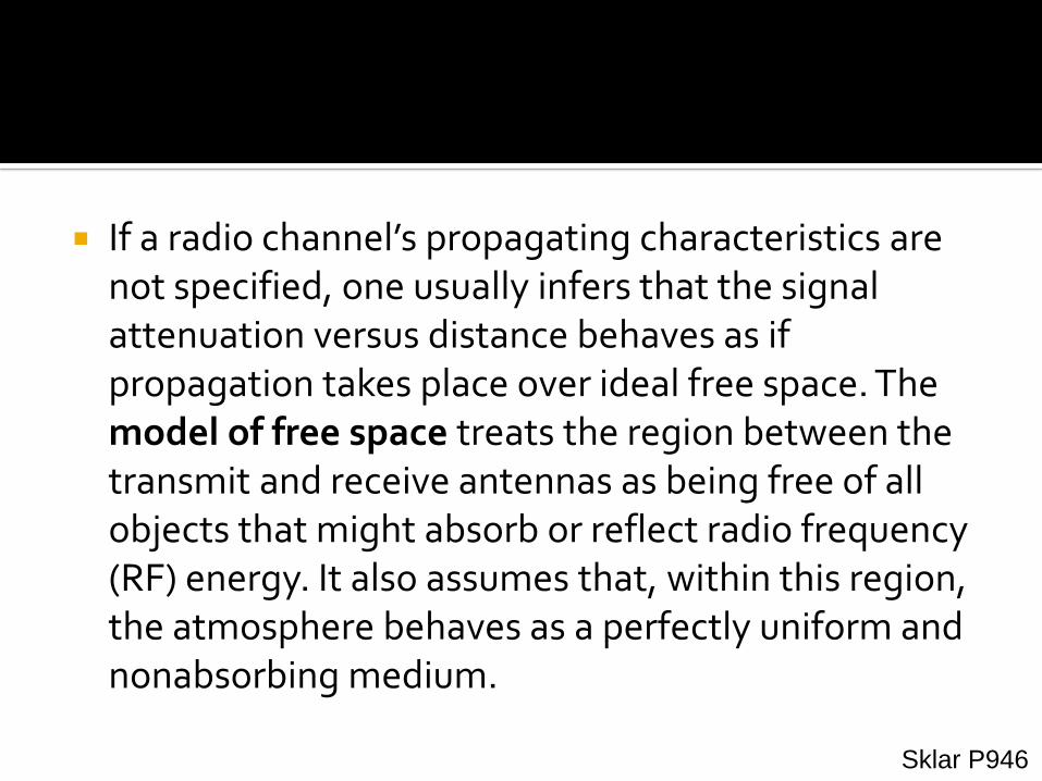
If a radio channel’s propagating characteristics are not specified, one usually infers that the signal attenuation versus distance behaves as if propagation takes place over ideal free space. The model of free space treats the region between the transmit and receive antennas as being free of all objects that might absorb or reflect radio frequency (RF) energy. It also assumes that, within this region, the atmosphere behaves as a perfectly uniform and nonabsorbing medium.

Sklar P946

Furthermore, the earth is treated as being infinitely far away from the propagating signal (or, equivalently, as having a reflection coefficient that is negligible). Basically, in this idealized free-space model, the attenuation of RF energy between the transmitter and receiver behaves according to an inverse-square law. The received power expressed in terms of transmitted power is attenuated by a factor , where this factor is called path loss or free space loss.

( )sL dSklar P946

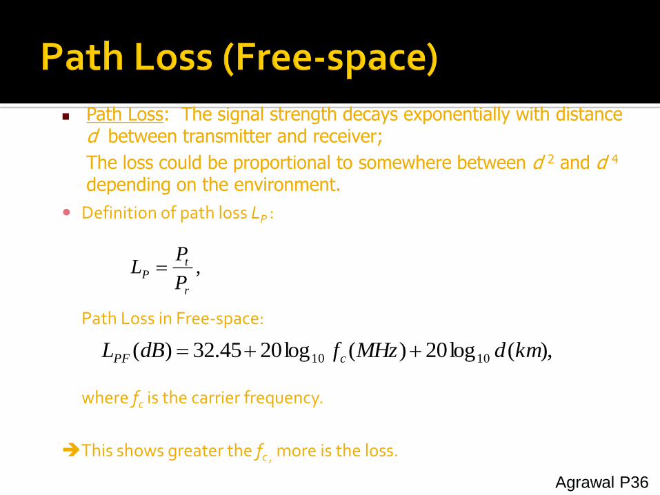
Path Loss: The signal strength decays exponentially with distance d between transmitter and receiver;

The loss could be proportional to somewhere between d 2 and d 4

depending on the environment.

Definition of path loss LP :

Path Loss in Free-space:

where fc is the carrier frequency.

This shows greater the fc , more is the loss.

,r

tP

P

PL

),(log20)(log2045.32)( 1010 kmdMHzfdBL cPF

Agrawal P36

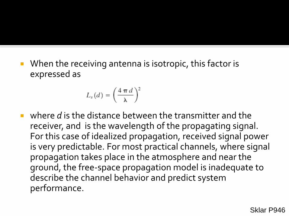
When the receiving antenna is isotropic, this factor is expressed as

where d is the distance between the transmitter and the receiver, and is the wavelength of the propagating signal. For this case of idealized propagation, received signal power is very predictable. For most practical channels, where signal propagation takes place in the atmosphere and near the ground, the free-space propagation model is inadequate to describe the channel behavior and predict system performance.

Sklar P946

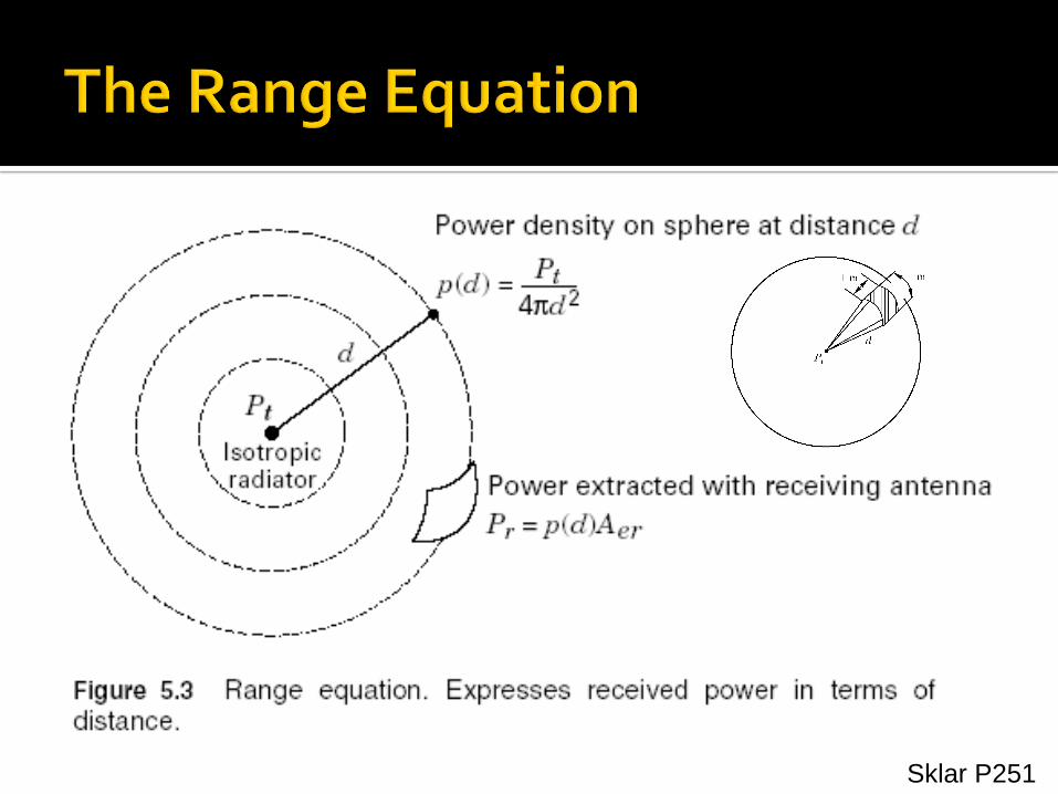
Sklar P251

Transmitter Distance d

Receiver

hb

hm

2r

4P

d

PGA tte

The received signal power at distance d:

where Pt is transmitting power, Ae is effective area, and Gt is the transmitting antenna gain. Assuming that the radiated power is uniformly distributed over the surface of the sphere.

Agrawal P35-36

Antenna gain

Power output, in a particular direction, compared to that produced in any direction by a perfect omnidirectional antenna (isotropic antenna)

Effective area

Related to physical size and shape of antenna

Stallings P98-99

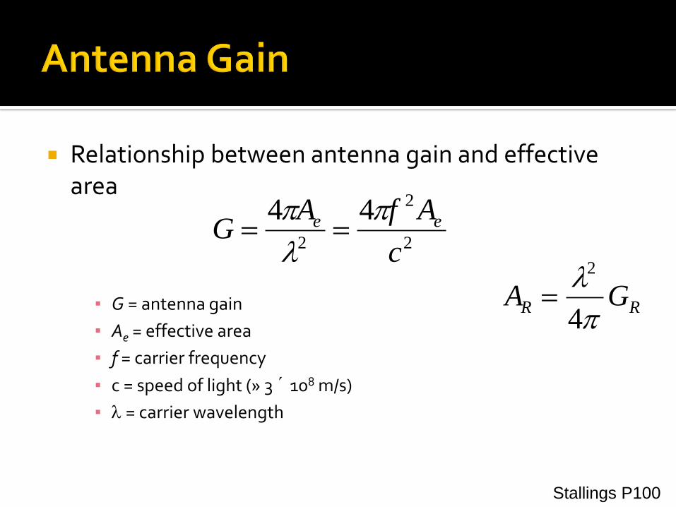
Relationship between antenna gain and effective area

▪ G = antenna gain

▪ Ae = effective area

▪ f = carrier frequency

▪ c = speed of light (» 3 ´ 108 m/s)

▪ = carrier wavelength

2

2

2

44

c

AfAG ee

Stallings P100

RR GA

4

2

Free space loss, ideal isotropic antenna

▪ Pt = signal power at transmitting antenna

▪ Pr = signal power at receiving antenna

▪ = carrier wavelength

▪ d = propagation distance between antennas

▪ c = speed of light (» 3 ´ 10 8 m/s)

where d and are in the same units (e.g., meters)

2

2

2

244

c

fdd

P

P

r

t

Stallings P106-107

H. T. Friis, "A note on a simple transmission formula," Proc.

IRE, vol. 34, pp. 254-256. 1946

Free space loss equation can be recast:

d

P

PL

r

tdB

4log20log10

dB 98.21log20log20 d

dB 56.147log20log204

log20

df

c

fd

Stallings P107

Free space loss accounting for gain of other antennas

▪ Gt = gain of transmitting antenna

▪ Gr = gain of receiving antenna

▪ At = effective area of transmitting antenna

▪ Ar = effective area of receiving antenna

trtrtrr

t

AAf

cd

AA

d

GG

d

P

P2

22

2

224

Stallings P107

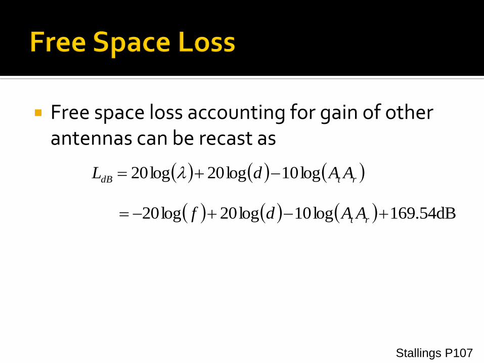
Free space loss accounting for gain of other antennas can be recast as

rtdB AAdL log10log20log20

dB54.169log10log20log20 rt AAdf

Stallings P107

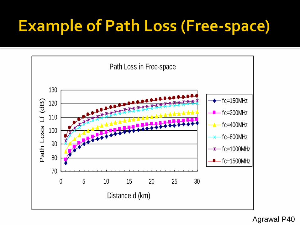
Path Loss in Free-space

70

80

90

100

110

120

130

0 5 10 15 20 25 30

Distance d (km)

Path

Loss L

f (d

B) fc=150MHz

fc=200MHz

fc=400MHz

fc=800MHz

fc=1000MHz

fc=1500MHz

Agrawal P40

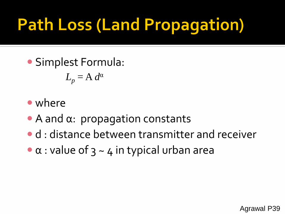
Simplest Formula: Lp = A dα

where

A and α: propagation constants

d : distance between transmitter and receiver

α : value of 3 ~ 4 in typical urban area

Agrawal P39

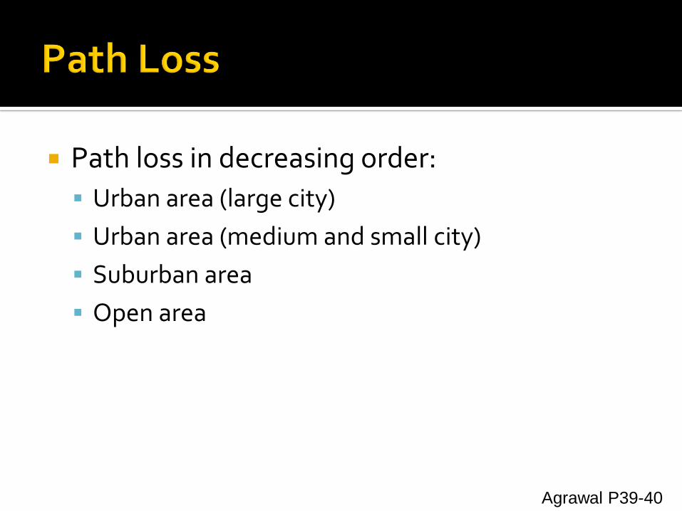
Path loss in decreasing order:

Urban area (large city)

Urban area (medium and small city)

Suburban area

Open area

Agrawal P39-40

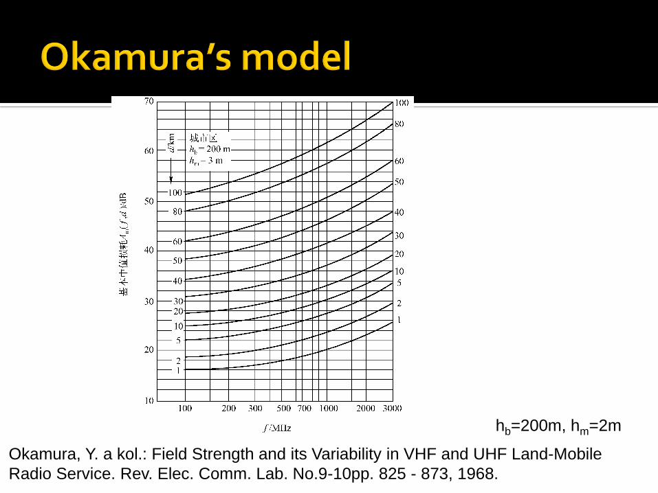
Okamura, Y. a kol.: Field Strength and its Variability in VHF and UHF Land-Mobile

Radio Service. Rev. Elec. Comm. Lab. No.9-10pp. 825 - 873, 1968.

hb=200m, hm=2m

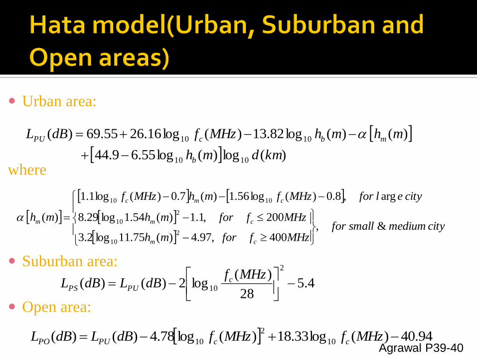
Urban area:

where

Suburban area:

Open area:

)(log)(log55.69.44

)()(log82.13)(log16.2655.69)(

1010

1010

kmdmh

mhmhMHzfdBL

b

mbcPU

citymediumsmallfor

MHzfformh

MHzfformh

cityelforMHzfmhMHzf

mh

cm

cm

cmc

m&,

400,97.4)(75.11log2.3

200,1.1)(54.1log29.8

arg,8.0)(log56.1)(7.0)(log1.1

)(

2

10

2

10

1010

4.528

)(log2)()(

2

10

MHzfdBLdBL c

PUPS

94.40)(log33.18)(log78.4)()( 10

2

10 MHzfMHzfdBLdBL ccPUPOAgrawal P39-40

Path Loss in Urban Area in Large City

100

110

120

130

140

150

160

170

180

0 10 20 30

Distance d (km)

Pa

th L

oss L

pu

(d

B)

fc=200MHz

fc=400MHz

fc=800MHz

fc=1000MHz

fc=1500MHz

fc=150MHz

Agrawal P40

Path Loss in Urban Area for Small & Medium Cities

100

110

120

130

140

150

160

170

180

0 10 20 30

Distance d (km)

Path

Loss L

pu (

dB

)

fc=150MHz

fc=200MHz

fc=400MHz

fc=800MHz

fc=1000MHz

fc=1500MHz

Agrawal P40

Path Loss in Suburban Area

90

100

110

120

130

140

150

160

170

0 5 10 15 20 25 30

Distance d (km)

Pa

th L

oss L

ps (

dB

)

fc=150MHz

fc=200MHz

fc=400MHz

fc=800MHz

fc=1000MHz

fc=1500MHz

Agrawal P40

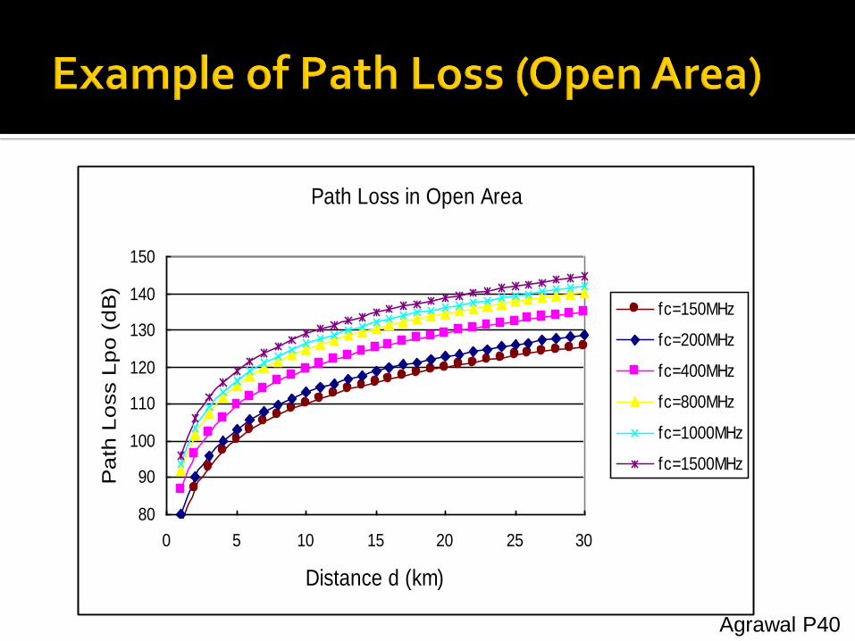
Path Loss in Open Area

80

90

100

110

120

130

140

150

0 5 10 15 20 25 30

Distance d (km)

Pa

th L

oss L

po

(d

B)

fc=150MHz

fc=200MHz

fc=400MHz

fc=800MHz

fc=1000MHz

fc=1500MHz

Agrawal P40

Rappaport P152

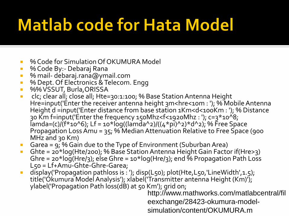
% Code for Simulation Of OKUMURA Model % Code By:- Debaraj Rana % mail- debaraj.rana@ymail.com % Dept. Of Electronics & Telecom. Engg %% VSSUT, Burla,ORISSA clc; clear all; close all; Hte=30:1:100; % Base Station Antenna Height

Hre=input('Enter the receiver antenna height 3m<hre<10m : '); % Mobile Antenna Height d =input('Enter distance from base station 1Km<d<100Km : '); % Distance 30 Km f=input('Enter the frequency 150Mhz<f<1920Mhz : '); c=3*10^8; lamda=(c)/(f*10^6); Lf = 10*log((lamda^2)/((4*pi)^2)*d^2); % Free Space Propagation Loss Amu = 35; % Median Attenuation Relative to Free Space (900 MHz and 30 Km)

Garea = 9; % Gain due to the Type of Environment (Suburban Area) Ghte = 20*log(Hte/200); % Base Station Antenna Height Gain Factor if(Hre>3)

Ghre = 20*log(Hre/3); else Ghre = 10*log(Hre/3); end % Propagation Path Loss L50 = Lf+Amu-Ghte-Ghre-Garea;

display('Propagation pathloss is : '); disp(L50); plot(Hte,L50,'LineWidth',1.5); title('Okumura Model Analysis'); xlabel('Transmitter antenna Height (Km)'); ylabel('Propagation Path loss(dB) at 50 Km'); grid on;

http://www.mathworks.com/matlabcentral/fil

eexchange/28423-okumura-model-

simulation/content/OKUMURA.m

Rappaport P139

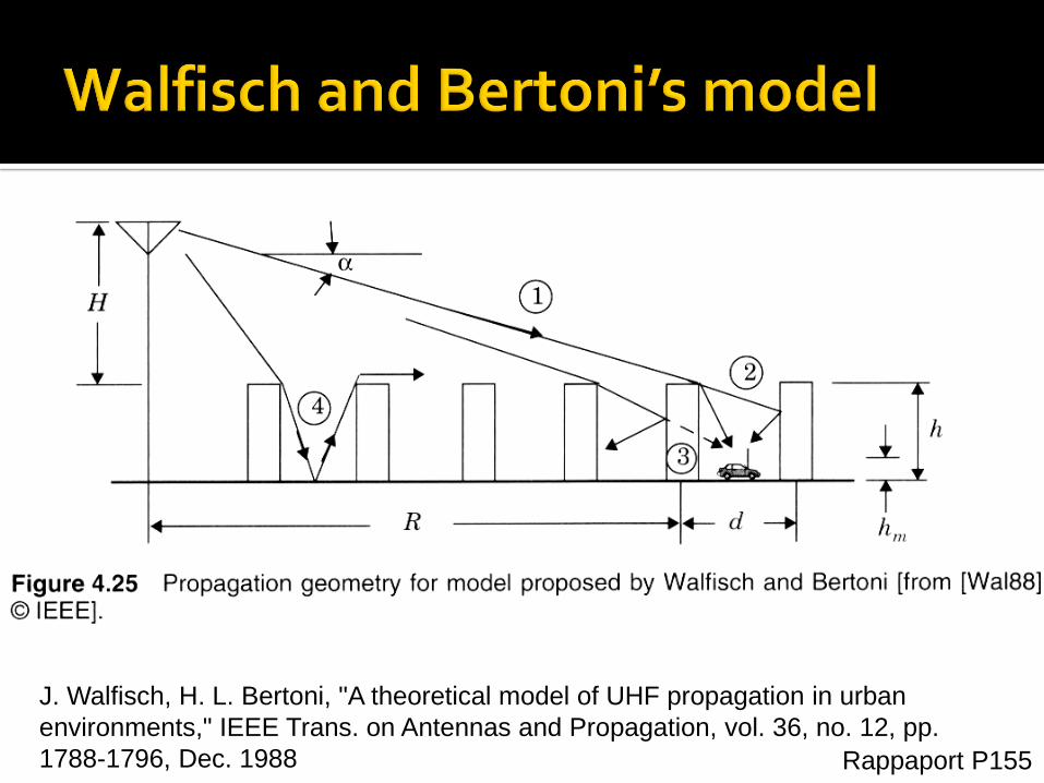
Rappaport P155

J. Walfisch, H. L. Bertoni, "A theoretical model of UHF propagation in urban

environments," IEEE Trans. on Antennas and Propagation, vol. 36, no. 12, pp.

1788-1796, Dec. 1988

Intermodulation noise – occurs if signals with different frequencies share the same medium

Interference caused by a signal produced at a frequency that is the sum or difference of original frequencies

Crosstalk – unwanted coupling between signal paths

Impulse noise – irregular pulses or noise spikes

Short duration and of relatively high amplitude

Caused by external electromagnetic disturbances, or faults and flaws in the communications system

Stallings P110

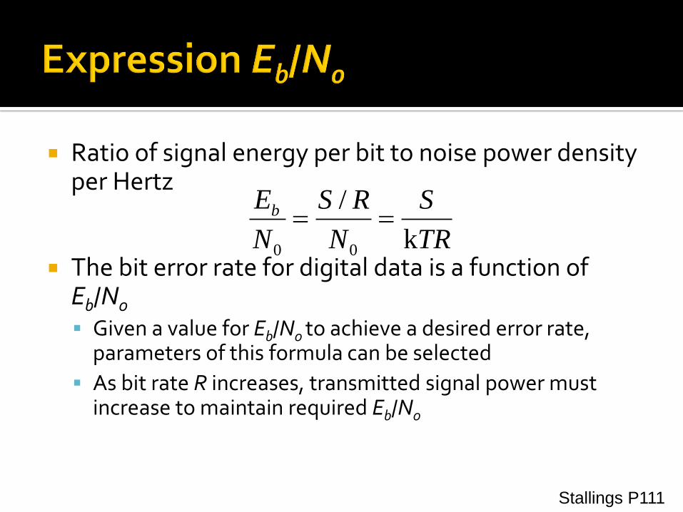
Ratio of signal energy per bit to noise power density per Hertz

The bit error rate for digital data is a function of Eb/N0

Given a value for Eb/N0 to achieve a desired error rate, parameters of this formula can be selected

As bit rate R increases, transmitted signal power must increase to maintain required Eb/N0

TR

S

N

RS

N

Eb

k

/

00

Stallings P111

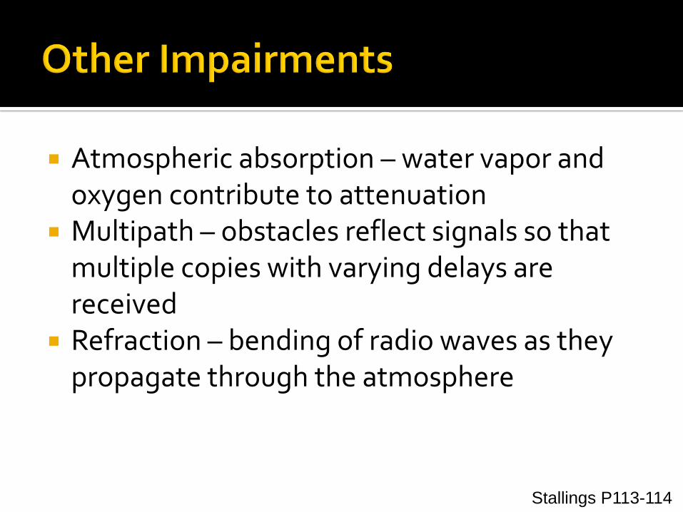
Atmospheric absorption – water vapor and oxygen contribute to attenuation

Multipath – obstacles reflect signals so that multiple copies with varying delays are received

Refraction – bending of radio waves as they propagate through the atmosphere

Stallings P113-114

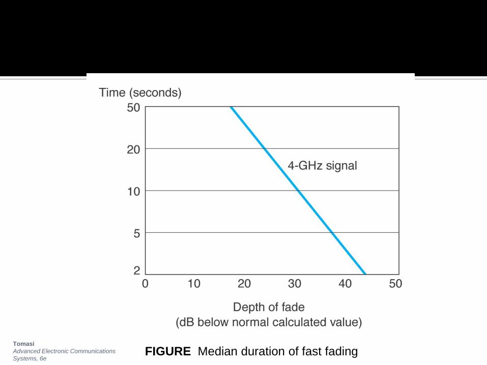
Tomasi

Advanced Electronic Communications

Systems, 6eFIGURE Median duration of fast fading

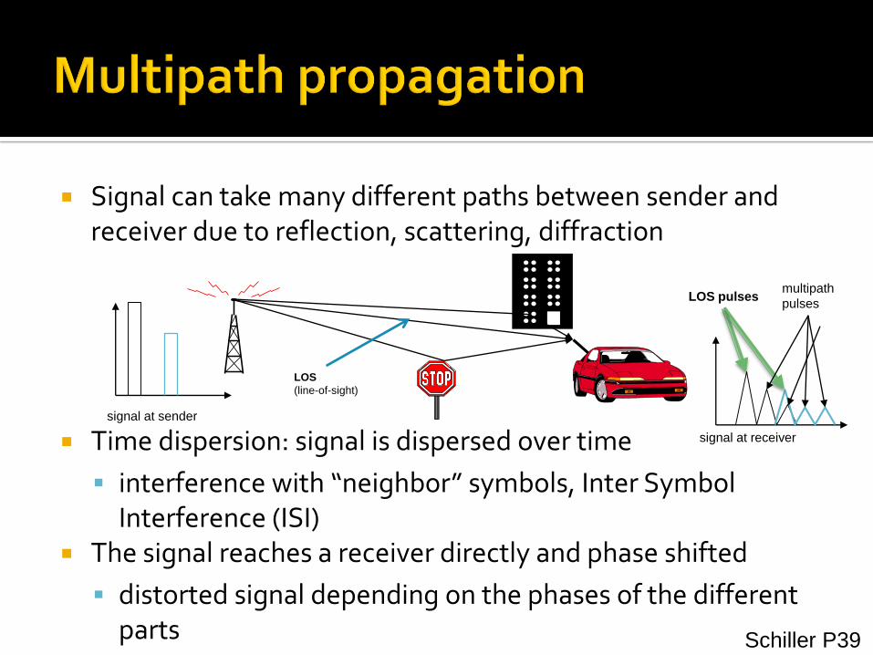
Signal can take many different paths between sender and receiver due to reflection, scattering, diffraction

Time dispersion: signal is dispersed over time

interference with “neighbor” symbols, Inter Symbol Interference (ISI)

The signal reaches a receiver directly and phase shifted

distorted signal depending on the phases of the different parts

signal at sender

signal at receiver

LOS pulsesmultipath

pulses

LOS

(line-of-sight)

Schiller P39

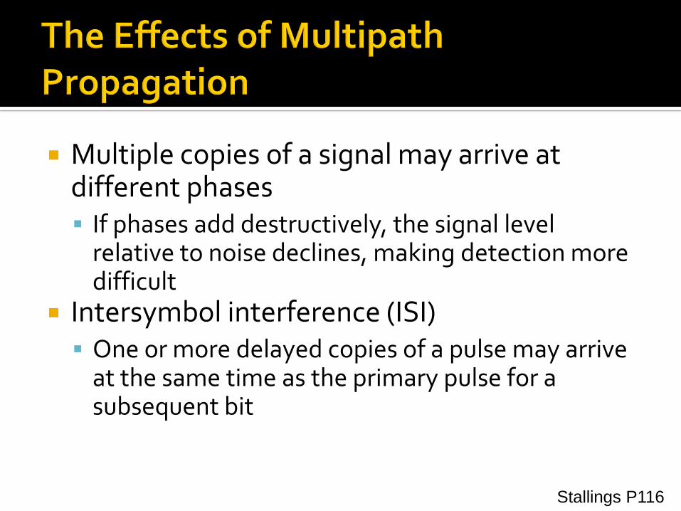
Multiple copies of a signal may arrive at different phases If phases add destructively, the signal level

relative to noise declines, making detection more difficult

Intersymbol interference (ISI) One or more delayed copies of a pulse may arrive

at the same time as the primary pulse for a subsequent bit

Stallings P116

Stallings P115

Figure Illustrating the mechanism of radio propagation

in urban areas. (From Parsons, 1992, with permission.)Haykin P532

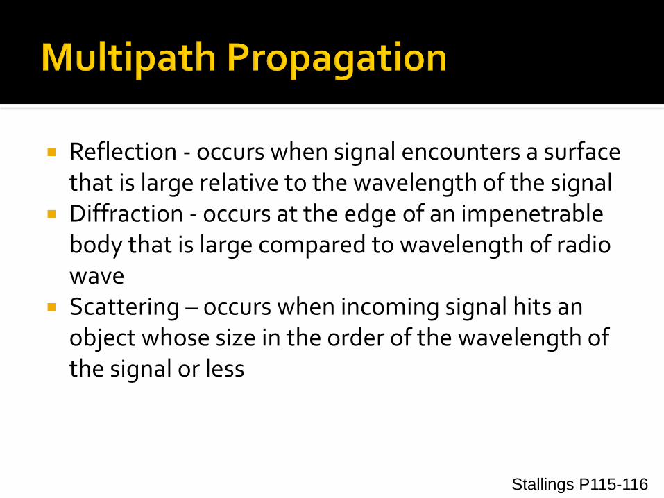
Reflection - occurs when signal encounters a surface that is large relative to the wavelength of the signal

Diffraction - occurs at the edge of an impenetrable body that is large compared to wavelength of radio wave

Scattering – occurs when incoming signal hits an object whose size in the order of the wavelength of the signal or less

Stallings P115-116

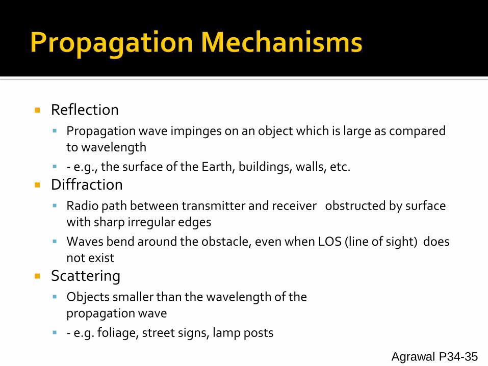
Reflection Propagation wave impinges on an object which is large as compared

to wavelength

- e.g., the surface of the Earth, buildings, walls, etc.

Diffraction Radio path between transmitter and receiver obstructed by surface

with sharp irregular edges

Waves bend around the obstacle, even when LOS (line of sight) does not exist

Scattering Objects smaller than the wavelength of the

propagation wave

- e.g. foliage, street signs, lamp posts

Agrawal P34-35

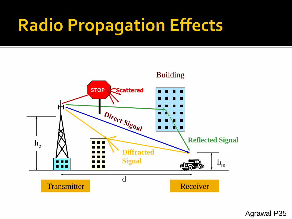
Transmitterd

Receiver

hb

hm

Diffracted

Signal

Reflected Signal

Building

STOP Scattered

Agrawal P35

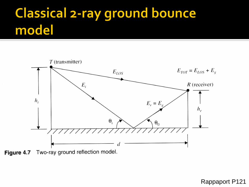
Rappaport P121

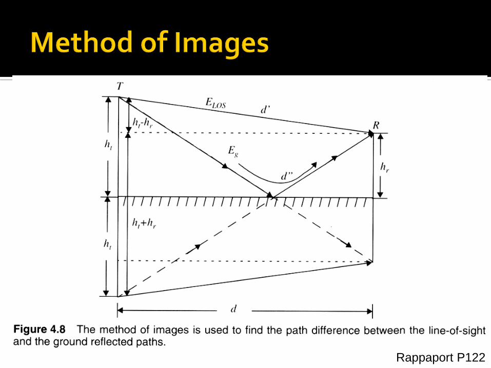
Rappaport P122

Rappaport P128

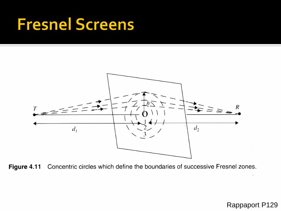
Rappaport P129

Figure 4.12 Illustration of Fresnel zones for different knife-edge diffraction scenarios. Rappaport P130

Ionosphere scattering

Frequency: 30 ~ 60 MHz

Troposphere scattering

Frequency: 100 ~ 4000 MHz

Meteor-tail scattering

Frequency: 30 ~ 100 MHz

Effective

scattering region

Transmitting

antenna EarthReceiving

antenna

Figure Troposphere scattering

communication

Ground

Figure Meteor-tail scattering

communication

Fan P15

Channel characteristics change over time and location signal paths change

different delay variations of different signal parts

different phases of signal parts

quick changes in the power received (short term fading)

Additional changes in distance to sender

obstacles further away

slow changes in the average power received (long term fading)

short term fading

long term

fading

t

power

Schiller P40

Fast fading Slow fading

Flat fading Selective fading

Rayleigh fading Rician fading

Stallings P117-118

Fast Fading

(Short-term fading)

Slow Fading

(Long-term fading)

Signal

Strength(dB)

Distance

Path Loss

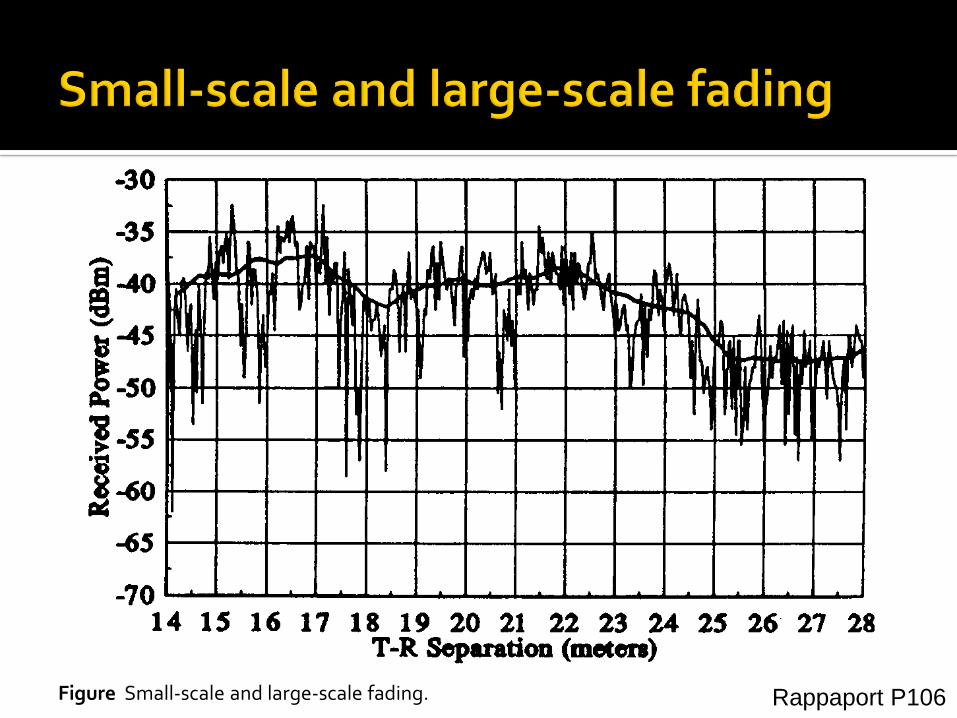
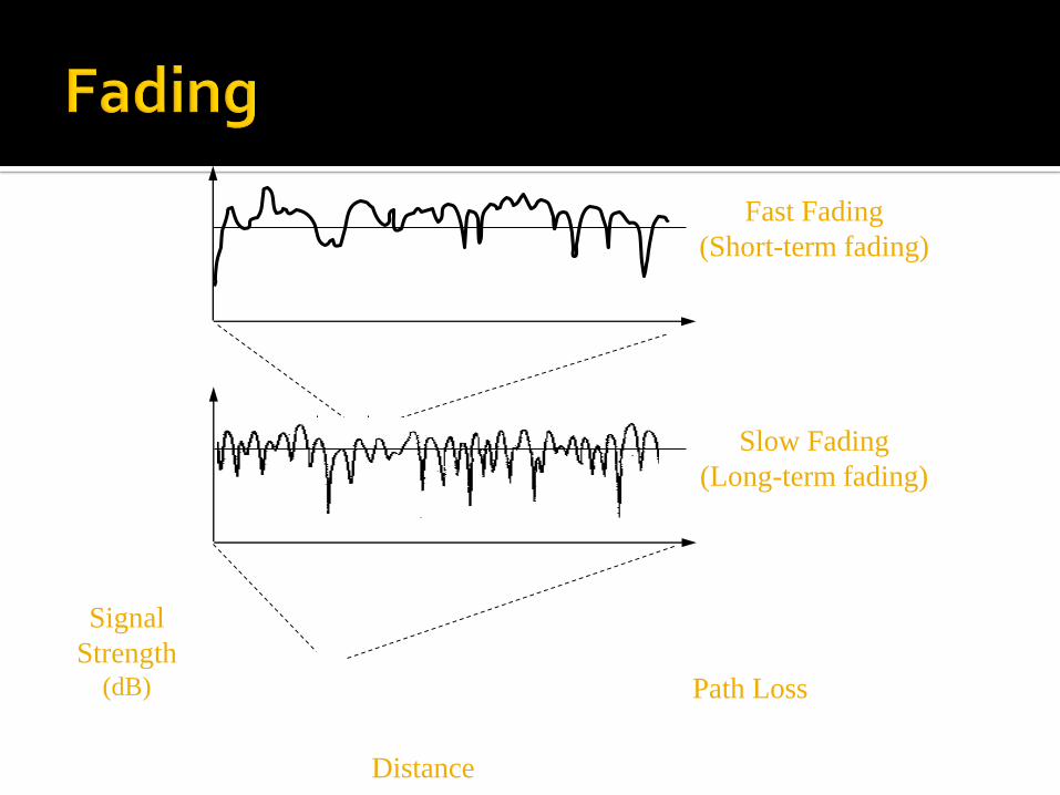
Figure Small-scale and large-scale fading. Rappaport P106

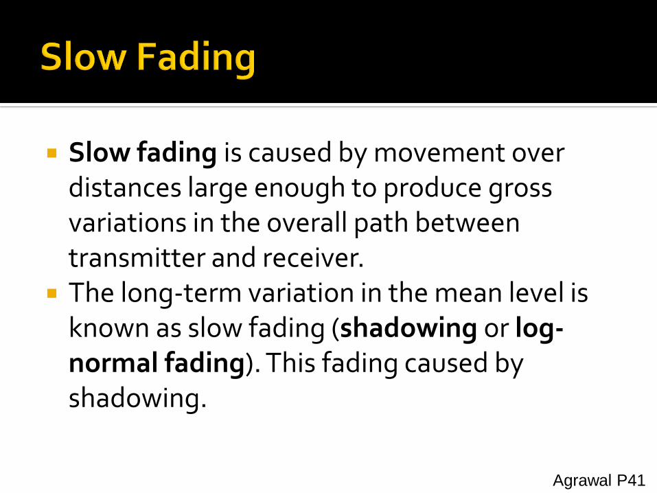
Slow fading is caused by movement over distances large enough to produce gross variations in the overall path between transmitter and receiver.

The long-term variation in the mean level is known as slow fading (shadowing or log-normal fading). This fading caused by shadowing.

Agrawal P41

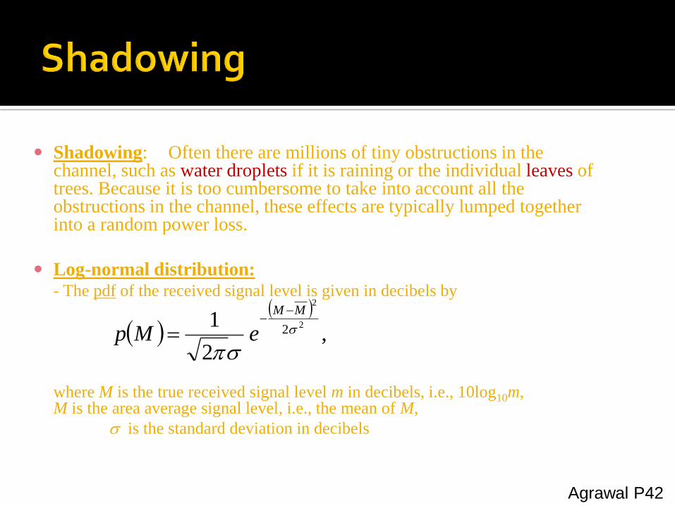
Shadowing: Often there are millions of tiny obstructions in the channel, such as water droplets if it is raining or the individual leaves of trees. Because it is too cumbersome to take into account all the obstructions in the channel, these effects are typically lumped together into a random power loss.

Log-normal distribution:- The pdf of the received signal level is given in decibels by

where M is the true received signal level m in decibels, i.e., 10log10m, M is the area average signal level, i.e., the mean of M,

is the standard deviation in decibels

,2

1 2

2

2

MM

eMp

Agrawal P42

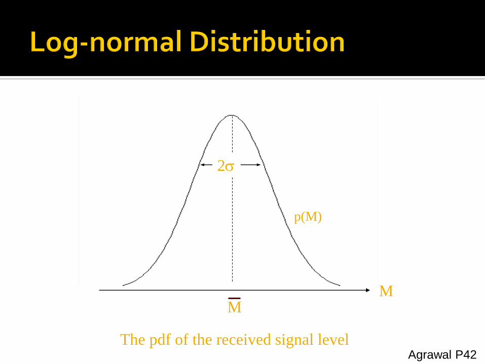
M

2

p(M)

M

The pdf of the received signal levelAgrawal P42

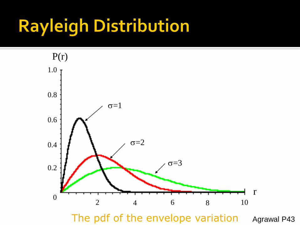
The signal from the transmitter may be reflected from objects such as hills, buildings, or vehicles. Fast fading is due to scattering of the signal by object near transmitter. When MS far from BS, the envelope distribution of received signal is

Rayleigh distribution with b=0. The pdf is

where is the standard deviation, r is the envelope of fading signal, b is the amplitude of direct signal, and I0 is the zero order Basel Function. Middle value rm of envelope signal within sample range to be satisfied

by

We have rm = 1.777

0),(20

22

2

22

rr

Ier

rp

r

b

b

.5.0)( mrrP

Agrawal P43

r2 4 6 8 10

P(r)

0

0.2

0.4

0.6

0.8

1.0

=1

=2

=3

The pdf of the envelope variation Agrawal P43

Rappaport P211

When MS is far from BS, the envelope distribution of received signal is called a Rician distribution. The pdf is

where

is the standard deviation,

I0(x) is the zero-order Bessel function of the first kind,

is the amplitude of the direct signal

0,02

2

2

22

rr

Ier

rp

r

Agrawal P44

r

Pdf

p(r

)

r86420

0.6

0.5

0.4

0.3

0.2

0.1

0

b = 2

b = 1

= 1

b = 3

b= 0 (Rayleigh)

The pdf of the envelope variationAgrawal P45

Rappaport P214

Level Crossing Rate:

Average number of times per second that the signal envelope crosses the level in positive going direction.

Fading Rate:

Number of times signal envelope crosses middle value in positive going direction per unit time.

Depth of Fading:

Ratio of mean square value and minimum value of fading signal.

Fading Duration:

Time for which signal is below given threshold.

Agrawal P46-47

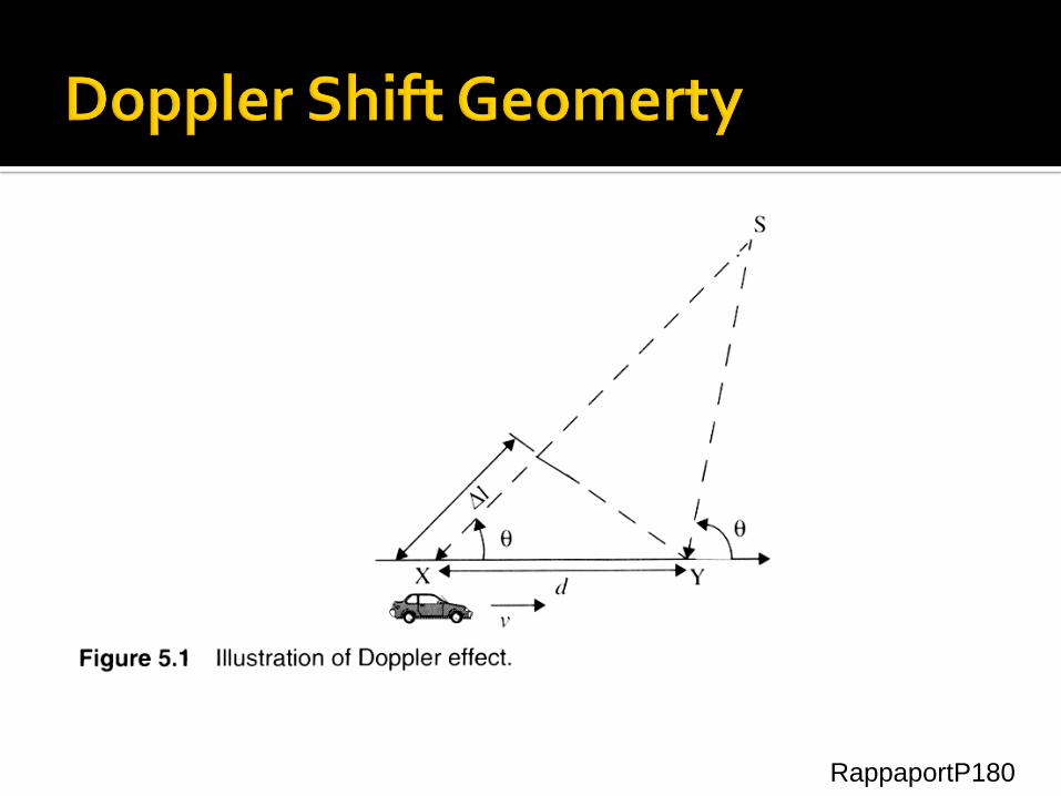
Doppler Effect: When a wave source and a receiver are moving towards each other, the frequency of the received signal will not be the same as the source.

When they are moving toward each other, the frequency of the received signal is higher than the source.

When they are opposing each other, the frequency decreases.

Thus, the frequency of the received signal is

where fC is the frequency of source carrier,

fD is the Doppler frequency.

Doppler Shift in frequency:

where v is the moving speed,

is the wavelength of carrier.

DCR fff

cosv

fD Signal

MSMoving

speed v

Agrawal P48-49

RappaportP180

Rappaport P219

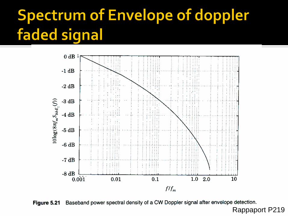
Rappaport P219

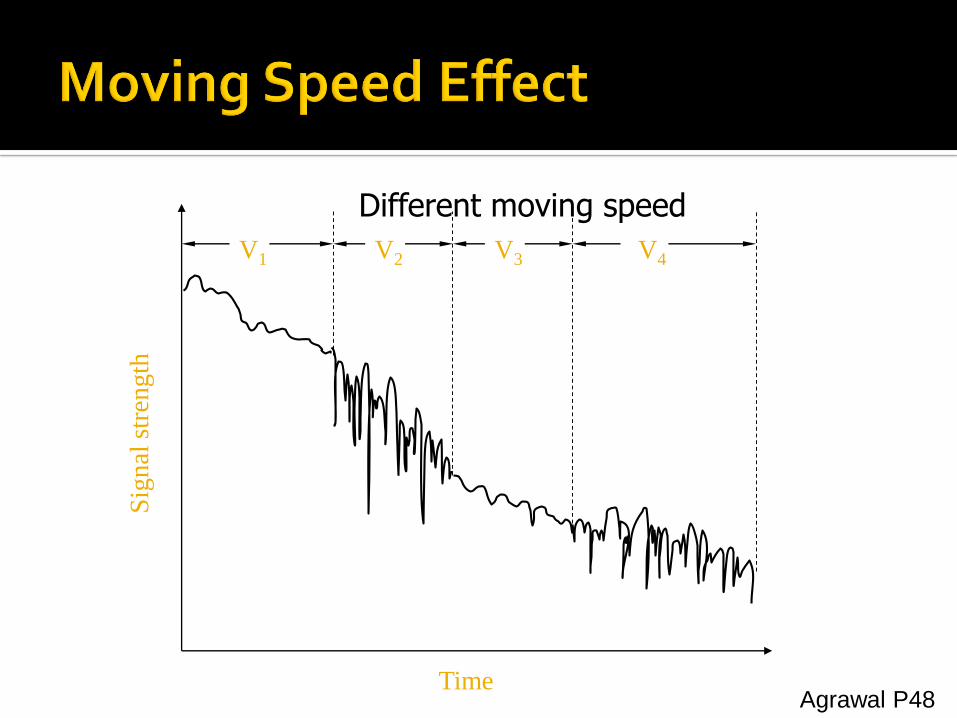
Time

V1 V2 V3 V4

Sig

nal

str

eng

th

Different moving speed

Agrawal P48

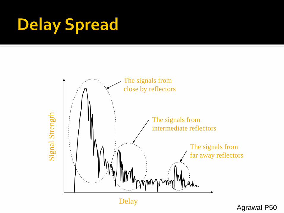
When a signal propagates from a transmitter to a receiver, signal suffers one or more reflections.

This forces signal to follow different paths. Each path has different path length, so the

time of arrival for each path is different. This effect which spreads out the signal is

called “Delay Spread”.

Agrawal P50

Delay

Sig

nal

Str

eng

th

The signals from

close by reflectors

The signals from

intermediate reflectors

The signals from

far away reflectors

Agrawal P50

Time

Time

Time

Received signal

(short delay)

Received signal

(long delay)

1

0

1

Propagation timeDelayed signals

Transmission

signal

Agrawal P51

Caused by time delayed multipath signals Has impact on the burst error rate of channel Second multipath is delayed and is received

during next symbol For low bit-error-rate (BER)

R (digital transmission rate) limited by delay spread d.

d

R2

1

Agrawal P51

Coherence bandwidth Bc:

Represents correlation between two fading signal envelopes at frequencies f1 and f2.

Is a function of delay spread.

Two frequencies that are larger than coherence bandwidth fade independently.

Concept useful in diversity reception

▪ Multiple copies of the same message are sent using different frequencies.

Agrawal P52

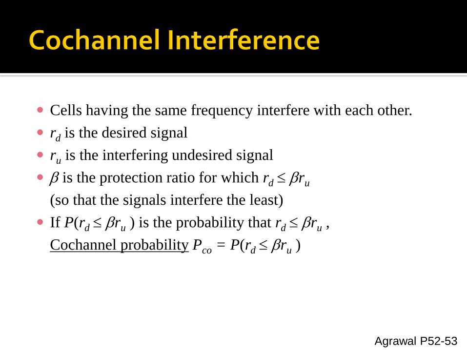
Cells having the same frequency interfere with each other.

rd is the desired signal

ru is the interfering undesired signal

b is the protection ratio for which rd bru

(so that the signals interfere the least)

If P(rd bru ) is the probability that rd bru ,

Cochannel probability Pco = P(rd bru )

Agrawal P52-53

Tomasi

Advanced Electronic Communications

Systems, 6e

FIGURE Co-channel interference

Tomasi

Advanced Electronic Communications

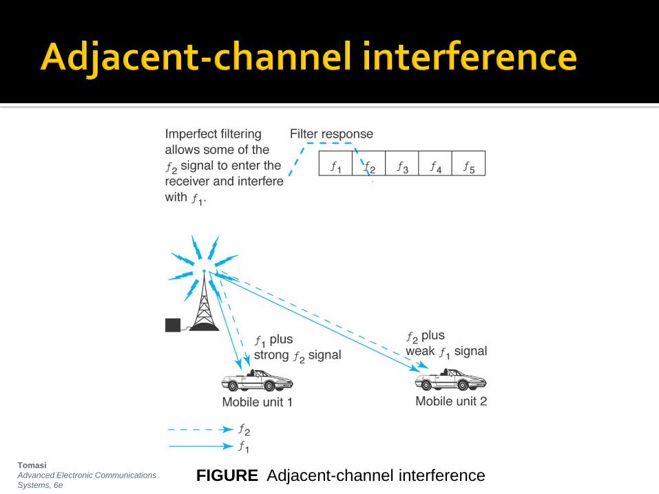
Systems, 6eFIGURE Adjacent-channel interference

Forward error correction Adaptive equalization Diversity techniques

Stallings P119-121

Transmitter adds error-correcting code to data block

Code is a function of the data bits

Receiver calculates error-correcting code from incoming data bits

If calculated code matches incoming code, no error occurred

If error-correcting codes don’t match, receiver attempts to determine bits in error and correct

Stallings P119-120

Can be applied to transmissions that carry analog or digital information Analog voice or video

Digital data, digitized voice or video Used to combat intersymbol interference Involves gathering dispersed symbol energy back

into its original time interval Techniques Lumped analog circuits

Sophisticated digital signal processing algorithms

Stallings P120

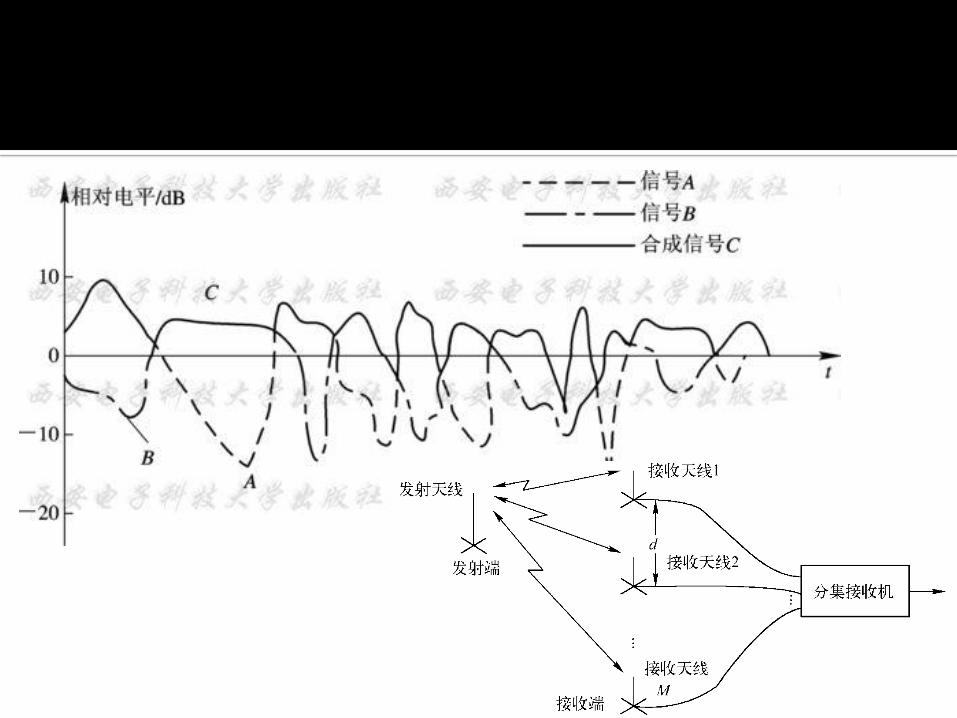
Diversity is based on the fact that individual channels experience independent fading events Space diversity – techniques involving physical

transmission path

Frequency diversity – techniques where the signal is spread out over a larger frequency bandwidth or carried on multiple frequency carriers

Time diversity – techniques aimed at spreading the data out over time

Stallings P120-121

Frequency and Spectrum Types of Waves Free-Space Propagation Path Loss Propagation Model Fading Doppler Shift Delay Spread

Stalling’s book P125 5.13 5.14