YPOTHESIS TESTING ARAMETRIC TESTS: TESTS ON MEANS

HYPOTHESIS TESTING

PARAMETRIC TESTS: TESTS ON MEANS

Sorana D. Bolboacă

©2015 - Sorana D. BOLBOACĂ 24-Nov-2015

OBJECTIVES Significance level vs. p-value

Hypothesis testing via confidence intervals

Hypothesis testing on a single mean

Comparisons of means on two samples (Student t-tests):

Independent sample tests

Dependent sample tests

Comparisons of more than two means: ANOVA test


P VALUES vs. CONFIDENCE INTERVALS

A P value measures the strength of evidence against the null hypothesis.

A P value is the probability of getting a result as, or more, extreme if the null hypothesis were true.

It is easy to compare results across studies using P values

P values are measures of statistical significance

Confidence intervals give a plausible range of values in clinically interpretable units

Confidence intervals enable easy assessment of clinical significance



Statistical significance can be obtained from a confidence interval as well as a hypothesis test

& Confidence intervals convey more information than p-values

For this reason, most medical journals now prefer that

results be presented with confidence intervals rather than p-values or both them.

If the NULL VALUE for a statistical hypothesis test using a significance level (alpha) = 0.05 is contained within the 95% confidence interval, we can conclude that there is NO statistical significance at alpha = 0.05 without doing the hypothesis test



For a 95% confidence interval for a difference between two values [-7.7 to 2.1]

The 95% CI includes 0, so there is no statistically significant difference between the values. In addition, we have information about the precision of our estimate of the difference, which cannot be obtained from p-values alone.

!!! This is a relatively wide confidence interval

maybe because the sample size is small


RELATION OF CONFIDENCE INTERVALS WITH

HYPOTHESIS TESTING

A general purpose approach to constructing confidence

intervals is to define a 100(1−α)% confidence interval to

consist of all those values θ0 for which a test of the

hypothesis θ=θ0 is not rejected at a significance level of

100α%.

Such an approach may not always be available since it

presupposes the practical availability of an appropriate

significance test.

Naturally, any assumptions required for the significance

test would carry over to the confidence intervals.


RELATION OF CONFIDENCE INTERVALS WITH

HYPOTHESIS TESTING

It may be convenient to make the general correspondence that parameter values within a confidence interval are equivalent to those values that would not be rejected by an hypothesis test, but this would be dangerous.

In many instances the confidence intervals that are quoted are only approximately valid, perhaps derived from "plus or minus twice the standard error", and the implications of this for the supposedly corresponding hypothesis tests are usually unknown.


HYPOTHESIS TESTING BY EXAMPLE

Null Hypothesis (H0): There is no difference between groups

There is no relationship between the independent and dependent variable(s).

Alternative hypothesis: There is a difference between groups

There is a relationship between the independent nd dependent variable(s).


The primary endpoint of the study is change in coronary flow reserve after the first 12 weeks' intervention.

The participants were consecutively enrolled during the inclusion

period and randomized (1:1) into two groups: 1. 12 weeks of AIT (aerobic interval training) three times a week,

followed by 40 weeks’AIT twice weekly. 2. 8–10 weeks’ LED (low energy diet) followed by 2–4 weeks of

transition to a high protein/low glycemic index diet and 40 weeks of weight loss maintenance and AIT twice weekly.

Null Hypothesis: The coronary flow reserve is not significantly different in AIT group compared to LED group.

Alternative hypothesis: The coronary flow reserve is significantly

different in AIT group compared to LED group.


HYPOTHESIS TESTING BY EXAMPLE Null and alternative hypotheses are either non-directional (two-tailed) or directional (one-tailed): Non-directional (two-tail): H0: Coronary flow reserved AIT = Coronary flow reserved LED H1/a: Coronary flow reserved AIT Coronary flow reserved LED

Directional (one-tail): H0: Coronary flow reserved AIT Coronary flow reserved LED or H0: Coronary

flow reserved AIT Coronary flow reserved LED

H1/a: Coronary flow reserved AIT > Coronary flow reserved LED or H1/a: Coronary

flow reserved AIT < Coronary flow reserved LED

Non-Rejection

Region

Rejection Region2.5%

Rejection Region2.5%

Non-

Rejection

Region

Rejection

Region

5.0%



Alpha () is the level of significance in hypothesis testing

Alpha is a probability specified before the test is

performed.

Alpha is the probability of rejecting the null hypothesis

when it is true.

By convention, typical values of alpha specified in medical

research are 0.05 and 0.01.

Alphas have corresponding critical values, the same ones

used to calculate confidence intervals – 0.05/1.96,

0.01/2.575



Beta () is the probability of accepting the

null hypothesis when it is false.

Typical values for beta are 0.10 to 0.20

Beta is directly related to the power of a statistical

test:

Power is the probability of correctly rejecting the null

hypothesis when it is false. Power = 1 - Beta

A type II error occurs when a false null hypothesis is

accepted.


P-VALUES

Are the actual probabilities calculated from a statistical test, and are compared against alpha to determine whether to reject the null hypothesis or not.

Example:

alpha = 0.05; calculated p-value = 0.008 reject null hypothesis

alpha = 0.05; calculated p-value = 0.110 fail to reject null hypothesis

A type I error occurs when a true null hypothesis is rejected.


True State of Nature

H0 True H0 False

Findings H0 True Correct Type II Error (β)

H0 False Type I Error (α) Correct

©2015 - Sorana D. BOLBOACĂ

SIGNIFICANCE LEVEL VS. p-VALUE

Significance level (α) = property of a statistical procedure and takes a fixed value. Usually take a value equal to 0.05

p-value = random variable whose value depends upon the composition of the individual sample

15

Materials and Methods

Results

24-Nov-2015


SIGNIFICANCE LEVEL VS. p-VALUE

16

http://www.ncbi.nlm.nih.gov/pmc/articles/PMC4129321/

24-Nov-2015

http://www.ncbi.nlm.nih.gov/pmc/articles/PMC4129321/


PARAMETRIC & NON-PARAMETRIC

Parametric Non-Parametric

Assumed distribution Normal Any

Assumed variance Homogenous Any

Type of data Ratio or Interval Ordinal or Nominal

Central measure Mean Median

Dispersion measure Standard deviation (Q1; Q3)

Parametric Non-Parametric

2 independent groups Independent t-test Mann-Whitney test

2 dependent groups Paired t-test Wilcoxon test

> 2 groups ANOVA Kruskal-Wallis test

Friedman’s ANOVA

Correlation Pearson Spearman, Kendall, etc.

… … …

24-Nov-2015


HYPOTHESIS

Null H0 Not significantly different ('=' symbol)

Alternative HA/H1 Significantly different

two-tail: '≠' symbol

one-tail: '<' OR '>' symbol

24-Nov-2015


HYPOTHESIS TESTING VIA CI n=33, m = 2.6, s = 1.2, SE = 0.21

95% CI for the average number exams failed by medical students in the first year of study is (1.7, 3.4). Based on this confidence interval, do these data support the hypothesis that medical students on average failed on average more than 2 exams?

H0 μ = 2 Medical student in first year of study failed 2 exams, on average

HA μ > 2 Medical student in first year of study failed more than 2 exams, on average

Always about population parameter, never about

population statistics 1.7 3.4

μ = 2

24-Nov-2015


HYPOTHESIS TESTING VIA CI n=33, m = 2.6, s = 1.2, SE = 0.21 P(observed or more extreme outcome|H0 true) P(m>2.6|H0: μ = 2) Test statistic: Z = (2.6-2)/0.21 = 2.8571 p-value = P(Z>2.8571) = 0.0021

p-value = the probability of observing data at least as favorable to the alternative hypothesis as our current data set, if the null hypothesis was true.

If p-value < 0.05 we say that it would be very unlikely to observe the data if the null hypothesis were true, and hence reject H0.

If the p-value > 0.05 we say that it is likely to observe the data even if the null hypothesis were true, and hence fail to reject H0.

24-Nov-2015

HYPOTHESIS TESTING MEANS

24-Nov-2015


HYPOTHESIS TESTING ON A SINGLE MEAN

1. Hypotheses: H0: μ = null value & HA: μ ≠ null value

2. Calculate the point estimator

3. Check conditions: Independence: observations are independent by each

others

Sample size: n ≥ 30

4. Draw sampling distribution, shade p-value, calculate test statistic: Z = (m- μ)/(s/√n)

5. Make a decision: p-value < α → reject H0 (data provide convincing evidence for

HA)

p-value > α → fail to reject H0 (data do not provide convincing evidence for HA)

24-Nov-2015


INDEPENDENT SAMPLES: ARE TWO MEANS

THE SAME?

Total sample size Subgroup sample size

Equal Variances

Unequal Variances

Large size (n>50 or n>100) or σ’s known

~ equal very different

Z-test Rank-sum test

Small size ~ equal very different

t-test Rank-sum test

Assumptions:

the observations are independent from each other;

the samples are drawn from a normal distribution (use a Rank-test when this assumption is violated);

standard deviation of samples are not statistically different by each other (apply an unequal variance form of the means test or a rank test).

23

24-Nov-2015


Z AND T TESTS TO COMPARE A SAMPLE MEAN WITH A

POPULATION MEAN

Z test

When? Population standard deviation is known OR n > 50 (100)

Hypotheses:

m = μ (H0) vs. m ≠ μ (H1)

Significance level (α = 0.05) → critical value with n-1 df (degree of freedom)

Test statistics:

z = (m-μ)/(σ/√n) where σ = standard deviation, n = sample size

t-test

16-Dec-2013

When? Unknown standard deviation OR n < 50 (100)

Hypotheses:

μ1= μ2 (H0) vs. μ1≠ μ2 (H1)

Significance level (α = 0.05) → critical value with n-1 df (degree of freedom)

Test statistics:

t = (m-μ)/(s/√n) where s = standard deviation, n = sample size

24

24-Nov-2015


Z AND T TESTS TO COMPARE A SAMPLE MEAN WITH A

POPULATION MEAN – PROBLEM 1

Z-test

μ = 0 (H0) vs μ ≠ 0 (H1)

α = 0.05

σ = 1.75

n = 15

m = 3.87

Zcrit = 1.96

Z statistic = ?

Conclusion ?

T-test

μ = 0 (H0) vs μ ≠ 0 (H1)

α = 0.05

s = 2.50

n = 15

m = 3.87

tcrit = 2.145

t statistic = ?

Conclusion ?

16-Dec-2013

25

24-Nov-2015


Z AND T TESTS TO COMPARE TWO SAMPLE MEANS

Z test

When? Population standard deviation is knows OR n > 50 (100)

Hypotheses:

μ1= μ2 (H0) vs. μ1≠ μ2 (H1)

Significance level (α = 0.05) → critical value with n1+n2-1 df (degree of freedom)

Test statistics:

z = (m1-m2)/σd, where σd = population standard error (σd = σ*sqrt(1/n1+1/n2))

t-test

When? Unknown standard deviation OR n < 50 (100)

Hypotheses:

μ1= μ2 (H0) vs. μ1≠ μ2 (H1)

Significance level (α = 0.05) → critical value with n1+n2-1 df (degree of freedom)

Test statistics:

t-statistics = (m1-m2)/sd, where sd = standard error

26

24-Nov-2015


INDEPENDENT SAMPLES T-TEST

Are the variances

statistically different?

t-test assuming unequal variances

t-test assuming equal variances

16-Dec-2013

27

24-Nov-2015


T TESTS TO COMPARE TWO SAMPLE MEANS

Age and prostate cancer t-test

Negative biopsy: n1=206, m1=66.59 years old, s1=8.21

Positive biopsy: n2=95, m2=67.14 years old, s2=7.88

σ = 8.10 (n=301)

α = 0.05 → tcritic = 1.96

sd = sqrt((1/206+1/95)×((204*8.212+94*7.882)/(205+95-2))) =

1.0055

t = (m1-m2)/sd = (66.59-67.14)/1.0055 = -0.5470 (p-value = 0.582)

-1.96 ≤ -0.5470 ≤ 1.96 → we failed to reject the H0 (The mean age

of subjects with positive biopsy is not significantly different by the

mean age of subjects with negative biopsy)

For samples > 100 the difference between Z and t-statistic is

negligible while the p-values are identical

16-Dec-2013

28

24-Nov-2015


STUDENT T-TEST FOR COMPARING TWO MEANS (UNKNOWN AND EQUAL VARIANCES)

Null hypothesis: Means difference of the two populations is not significantly different by zero.

Alternative hypothesis for two-tailed test: Means difference of the two populations is significantly different by equal.

Assumptions: The variables in the two samples are normal distributed The variances are equal

If these two assumptions are not satisfied the test loss its validity.

If the variances of populations are known the Z test is applied (is most powerful)

29

24-Nov-2015



Degree of freedom (df):

df = n1 + n2 - 2

Significance level: = 0.05

Critical region for two-tailed test

Statistics

;tt;

2;2nn

2;2nn 2121

21

21

n

1

n

1s

mmt

2 2

1 1 2 2

1 2

( 1) ( 1)

2

n s n ss

n n

30

24-Nov-2015



We want to study whether there is a significant difference between the amount of blood uric acid in women from urban and rural. In a sample of 16 women aged between 30 and 50 years in urban areas, average uric acid was 5 mg/100 ml, with a variance of 2 mg/100 ml. An average equal to 4 mg/100 ml with a variance of 2 mg/100 ml was obtained on a sample of 16 women aged 30 to 50 years in rural areas.

31

24-Nov-2015

Data: n1 = 16; n2 = 16 m1 = 5; m2 = 4 s2 = 2

Null hypothesis: The mean of uric acid in women from urban is not significantly different by the mean of acid in women from rural.

Alternative hypothesis (two-tail test): The mean of uric acid in women from urban is not significantly different by the mean of acid in women from rural.



Degree of freedom: df = n1+n2-2 =16+16-2=30

Significance level: = 0.05.

Critical region for bilateral test: );04.2[]04.2;(

32

24-Nov-2015

Conclusion:

Statistical: The null hypothesis is fail to be rejected since the statistics did not belongs to the critical region.

Clinical: The serum level of uric acid is not significantly different in women from rural compared to those from urban areas.

68.15937.0

1

3525.0

1

25.041.1

1

16

1

16

141.1

45

n

1

n

1s

mmt

21

21

41.130

60

21616

2)116(2)116(

2nn

s)1n(s)1n(s

21

222

211



24-Nov-2015


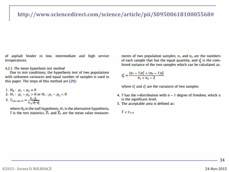
http://www.sciencedirect.com/science/article/pii/S0950061810005568#

34

24-Nov-2015


PAIRED SAMPLES STUDENT T-TEST FOR COMPARING MEANS

Aim: comparing the means of two paired samples on quantitative continuous variable (paired means the observation of the same quantitative variable before and after the action of a factor)

Assumptions:

Individual observations from the first sample corresponds to a pair in the second sample

The differences between pairs of values are normally distributed.

Null hypothesis: The difference of means is not significantly different by zero.

Alternative hypothesis (two-tail): The difference of means is significantly different by zero.

16-Dec-2013

35

24-Nov-2015


STUDENT (T) FOR COMPARING MEANS OF PAIRED SAMPLES

Degrees of freedom (df): df = n – 1


Critical region:

Statistics

s = standard deviation of the differences

n = sample size

);t[]t;(2

;1n2

;1n

n

s

dt

n

d...ddd n21

16-Dec-2013

36

24-Nov-2015

d1 = the difference between paired data for the first subject

The mean of the difference of paired data


PAIRED STUDENT T-TEST

16-Dec-2013

37

24-Nov-2015


PAIRED STUDENT T-TEST

16-Dec-2013

38

24-Nov-2015


STUDENT T-TEST FOR COMPARING MEANS OF PAIRED SAMPLES

Null hypothesis: There is no significant difference in systolic blood pressure before and after using of oral contraceptives.

Alternative hypothesis for two-tailed test: There is a significant difference in systolic blood pressure before and after using of oral contraceptives.

Degrees of freedom: df = n – 1 = 10-1 = 9


Critical regions for two-tailed test: (-∞; -2.262] [2.262; +∞)

16-Dec-2013

39

24-Nov-2015


STUDENT T-TEST FOR COMPARING MEANS OF PAIRED SAMPLES

Conclusion (two-sided test):

Statistical: The null hypothesis is rejected since the statistics belongs to critical region.

Clinical: The use of oral contraceptives is associated to a significant increase in systolic blood pressure.

16-Dec-2013

57.484.209

60.187

110

84.724.4664.044.184.42)2.4(64.3324.324.67s

2

8.410

48

10

22467791313d

15.352.1

8.4

3

57.48.4

9

57.48.4

n

sd

t

40

24-Nov-2015


THREE OR MORE MEANS: ANOVA

Are the means of k groups different?

H0: There are no differences among the mi.

H1: A difference exists somewhere among the groups

Is the t-test appropriate?

No, because the t-test compare two groups and this approach will increase the size of the error as the number of groups is higher than 2 instead of 5%

24-Nov-2015



Solution: apply ANOVA (analysis of variance, one-factor ANOVA or one-way ANOVA)

ANOVA Assumptions:

data are independent from each other;

distribution of each group in original data is normal;

the variances are not significantly different by each other

42

24-Nov-2015



Hypotheses: H0: There are no differences among means

H1: There are one or more differences somewhere among means

Verify assumptions: normal distribution; not statistically different variances

α = 0.05 – df = k-1 (numerator) and df = n-k (denominator)

F = MSM/MSE

If F > Fcrit → reject H0; F < Fcrit → failed to reject H0

24-Nov-2015

Source of variability

Sum of Squares Mean of squares

Abb Formula df Abb Formula

Mean SSM ∑k ni·(mi-m)2 k-1 MSM SSM/(k-1)

Error SSE SST – SSM n-k MSE SSE/(n-k)

Total SST ∑n(xi-m)2 n-1 MST SST/(n-1)


THREE OR MORE MEANS: ANOVA - PROBLEM

α=0.05; df: k-1=3-1=2; n-k=301-3=298; Fcrit = 3.03; m = 66.8; SST = 19670.3; MST = 65.57

24-Nov-2015

PSA CaP risk group n m s

< 4 ng/ml Low 89 66.1 9.1

4−10 ng/ml Uncertain 164 66.3 7.8

>10 ng/ml High 48 69.6 6.4

PSA=prostate-specific antigen; CaP = prostate cancer; n = sample size; m = mean; s = standard deviation

Source of variability

Sum of Squares Mean of squares

Abb Formula df Abb Formula

Mean SSM ∑k ni·(mi-m)2 k-1 MSM SSM/(k-1)

Error SSE SST – SSM n-k MSE SSE/(n-k)

Total SST ∑n(xi-m)2 n-1 MST SST/(n-1)


THREE OR MORE MEANS: ANOVA - PROBLEM

SSM = ∑k ni·(mi-m)2 = 89*(66.1-66.8)^2+ 164*(66.3-66.8)^2+ 48*(69.6-66.8)^2 = 460.93

MSM = SSM/2 = 460.93/2 = 230.47

SSE =SST-SSM = 19670.3 - 460.93 = 19209.37

MSE = SSE/298 = 19209.37/298 = 64.46

F = MSM/MSE = 230.47/64.46 = 3.58

Since 3.58 > 3.03 → a difference among means exists

24-Nov-2015

PSA CaP risk group n m s

< 4 ng/ml Low 89 66.1 9.1

4−10 ng/ml Uncertain 164 66.3 7.8

>10 ng/ml High 48 69.6 6.4

PSA=prostate-specific antigen; CaP = prostate cancer; n = sample size; m = mean; s = standard deviation


http://www.hindawi.com/journals/tswj/2013/608683/tab2/

46

TESTS ON MEANS BY EXAMPLES

24-Nov-2015




47

24-Nov-2015



Thank you for your attention!

24-Nov-2015


http://www.philosophers.co.uk/brain.jpg

YPOTHESIS TESTING ARAMETRIC TESTS: TESTS ON MEANS

Documents

Transcript of YPOTHESIS TESTING ARAMETRIC TESTS: TESTS ON MEANS