[York University, Swishchuk Modeling of Variance and Volatility Swaps for Financial Markets With...
19
Modeling of Variance and Volatility Swaps for Financial Markets with Stochastic Volatilities Anatoliy Swishchuk Department of Mathematics & Statistics York University, 4700 Keele str. Toronto, ON Canada M3J 1P3 E-mail: aswishch @mathsta t.yorku.ca Home pa ge: www.math.yorku.ca/˜aswishch Abstract. A new probabilistic approach is proposed to study variance and volatility swaps for financial markets with underlying asset and variance that follow the Heston (1993) model. W e also study covariance and corre lation swaps for the financial markets. As an application, we provide a numerical example using S &P 60 Canada Index to price swap on the volatility. 1 Introducti on. In the early 1970’s, Black and Scholes (1973) made a major breakthrough by deriving pricing formulas for vanilla options written on the stock. The Black- Scholes model assumes that the volatility term is a constant. This assumption is not always satisfied by real-life options as the probability distribution of an equity has a fatter left tail and thinner right tail than the lognormal distribution (see Hull (2000)), and the assumption of constant volatility σ in financial model (such as the original Black-Scholes model) is incompatible with derivatives prices observed in the market. The above issues have been addressed and studied in several ways, such as: (i) Volatility is assumed to be a deterministic function of the time: σ ≡ σ(t) (se e Wilmot t et al. (19 95) ); Merton (19 73) exte nde d the term structu re of volatility to σ := σ t (deterministic function of time), with the implied volatility for an option of maturity T given by ˆ σ 2 T = 1 T T 0 σ 2 u du; (ii) Volatility is assumed to be a function of the time and the current level of the stock price S (t): σ ≡ σ(t, S (t)) (see Hull (2000)); the dynamics of the stock price satisfies the following stochastic differential equation: dS (t) = µS (t)dt + σ(t, S (t))S (t)dW 1 (t), where W 1 (t) is a standard Wiener process; 1
Transcript of [York University, Swishchuk Modeling of Variance and Volatility Swaps for Financial Markets With...
8/6/2019 [York University, Swishchuk Modeling of Variance and Volatility Swaps for Financial Markets With Stochastic Volatility
http://slidepdf.com/reader/full/york-university-swishchuk-modeling-of-variance-and-volatility-swaps-for-financial 1/19
Modeling of Variance and Volatility Swaps forFinancial Markets with Stochastic Volatilities
Anatoliy SwishchukDepartment of Mathematics & StatisticsYork University, 4700 Keele str.Toronto, ON Canada M3J 1P3 E-mail: [email protected] Home page: www.math.yorku.ca/˜aswishch
Abstract.
A new probabilistic approach is proposed to study variance and volatilityswaps for financial markets with underlying asset and variance that followthe Heston (1993) model. We also study covariance and correlation swapsfor the financial markets. As an application, we provide a numerical exampleusing S &P 60 Canada Index to price swap on the volatility.
1 Introduction.
In the early 1970’s, Black and Scholes (1973) made a major breakthrough byderiving pricing formulas for vanilla options written on the stock. The Black-Scholes model assumes that the volatility term is a constant. This assumptionis not always satisfied by real-life options as the probability distribution of an equity has a fatter left tail and thinner right tail than the lognormaldistribution (see Hull (2000)), and the assumption of constant volatility σin financial model (such as the original Black-Scholes model) is incompatiblewith derivatives prices observed in the market.
The above issues have been addressed and studied in several ways, suchas:(i) Volatility is assumed to be a deterministic function of the time: σ ≡ σ(t)(see Wilmott et al. (1995)); Merton (1973) extended the term structure
of volatility to σ := σt (deterministic function of time), with the impliedvolatility for an option of maturity T given by σ2
T = 1T
T
0σ2
udu;(ii) Volatility is assumed to be a function of the time and the current levelof the stock price S (t): σ ≡ σ(t, S (t)) (see Hull (2000)); the dynamics of thestock price satisfies the following stochastic differential equation:
dS (t) = µS (t)dt + σ(t, S (t))S (t)dW 1(t),
where W 1(t) is a standard Wiener process;
1
8/6/2019 [York University, Swishchuk Modeling of Variance and Volatility Swaps for Financial Markets With Stochastic Volatility
http://slidepdf.com/reader/full/york-university-swishchuk-modeling-of-variance-and-volatility-swaps-for-financial 2/19
(iii) The time variation of the volatility involves an additional source of ran-domness, besides W 1(t), represented by W 2(t), and is given by
dσ(t) = a(t, σ(t))dt + b(t, σ(t))dW 2(t),
where W 2(t) and W 1(t) (the initial Wiener process that governs the priceprocess) may be correlated (see Buff (2002), Hull and White (1987), Heston(1993));(iv) The volatility depends on a random parameter x such as σ(t) ≡ σ(x(t)),where x(t) is some random process (see Elliott and Swishchuk (2002), Griegoand Swishchuk (2000), Swishchuk (1995), Swishchuk (2000), Swishchuk et al.(2000));(v) Another approach is connected with stochastic volatility, namely, un-certain volatility scenario (see Buff (2002)). This approach is based on theuncertain volatility model developed in Avellaneda et al. (1995), where a
concrete volatility surface is selected among a candidate set of volatility sur-faces. This approach addresses the sensitivity question by computing anupper bound for the value of the portfolio under arbitrary candidate volatil-ity, and this is achieved by choosing the local volatility σ(t, S (t)) among twoextreme values σmin and σmax such that the value of the portfolio is maximizedlocally;
(vi) The volatility σ(t, S t) depends on S t := S (t + θ) for θ ∈ [−τ, 0],namely, stochastic volatility with delay (see Kazmerchuk, Swishchuk andWu (2002));
In the approach (i), the volatility coefficient is independent of the cur-rent level of the underlying stochastic process S (t). This is a deterministic
volatility model, and the special case where σ is a constant reduces to thewell-known Black-Scholes model that suggests changes in stock prices arelognormal distributed. But the empirical test by Bollerslev (1986) seems toindicate otherwise. One explanation for this problem of a lognormal modelis the possibility that the variance of log(S (t)/S (t − 1)) changes randomly.This motivated the work of Chesney and Scott (1989), where the prices areanalyzed for European options using the modified Black-Scholes model of foreign currency options and a random variance model. In their works theresults of Hull and White (1987), Scott (1987) and Wiggins (1987) were usedin order to incorporate randomly changing variance rates.
In the approach (ii), several ways have been developed to derive thecorresponding Black-Scholes formula: one can obtain the formula by usingstochastic calculus and, in particular, the Ito’s formula (see Øksendal (1998),for example).
A generalized volatility coefficient of the form σ(t, S (t)) is said to belevel-dependent . Because volatility and asset price are perfectly correlated,we have only one source of randomness given by W 1(t). A time and level-dependent volatility coefficient makes the arithmetic more challenging andusually precludes the existence of a closed-form solution. However, the ar-
2
8/6/2019 [York University, Swishchuk Modeling of Variance and Volatility Swaps for Financial Markets With Stochastic Volatility
http://slidepdf.com/reader/full/york-university-swishchuk-modeling-of-variance-and-volatility-swaps-for-financial 3/19
bitrage argument based on portfolio replication and a completeness of themarket remain unchanged.
The situation becomes different if the volatility is influenced by a second“non-tradable” source of randomness. This is addressed in the approach(iii), (iv) and (v) we usually obtains a stochastic volatility model , which isgeneral enough to include the deterministic model as a special case. Theconcept of stochastic volatility was introduced by Hull and White (1987),and subsequent development includes the work of Wiggins (1987), Johnsonand Shanno (1987), Scott (1987), Stein and Stein (1991) and Heston (1993).We also refer to Frey (1997) for an excellent survey on level-dependent andstochastic volatility models. We should mention that the approach (iv) istaken by, for example, Griego and Swishchuk (2000).
Hobson and Rogers (1998) suggested a new class of non-constant volatilitymodels, which can be extended to include the aforementioned level-dependentmodel and share many characteristics with the stochastic volatility model.
The volatility is non-constant and can be regarded as an endogenous factorin the sense that it is defined in terms of the past behaviour of the stockprice. This is done in such a way that the price and volatility form a multi-dimensional Markov process. Volatility swaps are forward contracts on futurerealized stock volatility, variance swaps are similar contract on variance, thesquare of the future volatility, both these instruments provide an easy wayfor investors to gain exposure to the future level of volatility.
A stock’s volatility is the simplest measure of its risk less or uncertainty.Formally, the volatility σR is the annualized standard deviation of the stock’sreturns during the period of interest, where the subscript R denotes theobserved or ”realized” volatility.
The easy way to trade volatility is to use volatility swaps, sometimescalled realized volatility forward contracts, because they provide pure expo-sure to volatility(and only to volatility).
Demeterfi, K., Derman, E., Kamal, M., and Zou, J. (1999) explained theproperties and the theory of both variance and volatility swaps. They derivedan analytical formula for theoretical fair value in the presence of realisticvilatility skews, and pointed out that volatility swaps can be replicated bydynamically trading the more straightforward variance swap.
Javaheri A, Wilmott, P. and Haug, E. G. (2002) discussed the valuationand hedging of a GARCH(1,1) stochastic volatility model. They used a
general and exible PDE approach to determine the first two moments of therealized variance in a continuous or discrete context. Then they approximatethe expected realized volatility via a convexity adjustment.
Brockhaus and Long (2000) provided an analytical approximation forthe valuation of volatility swaps and analyzed other options with volatilityexposure.
Working paper by Theoret, Zabre and Rostan (2002) presented an analyt-ical solution for pricing of volatility swaps, proposed by Javaheri, Wilmottand Haug (2002). They priced the volatility swaps within framework of
3
8/6/2019 [York University, Swishchuk Modeling of Variance and Volatility Swaps for Financial Markets With Stochastic Volatility
http://slidepdf.com/reader/full/york-university-swishchuk-modeling-of-variance-and-volatility-swaps-for-financial 4/19
GARCH(1,1) stochastic volatility model and applied the analytical solutionto price a swap on volatility of the S &P 60 Canada Index (5-year historicalperiod: 1997− 2002).
In the paper we propose a new probabilistic approach to the study of stochastic volatility model (Section 3), Heston (1993) model, to model vari-ance and volatility swaps (Section 2). The Heston asset process has a vari-ance σ2
t that follows a Cox, Ingersoll & Ross (1985) process. We find someanalytical close forms for expectation and variance of the realized both con-tinuously (Section 3.4) and discrete sampled variance (Section 3.5), whichare needed for study of variance and volatility swaps, and price of pseudo-variance, pseudo-volatility, the problems proposed by He & Wang (2002) forfinancial markets with deterministic volatility as a function of time. This ap-proach was first applied to the study of stochastic stability of Cox-Ingersoll-Ross process in Swishchuk and Kalemanova (2000).
The same expressions for E [V ] and for V ar[V ] (like in present paper)
were obtained by Brockhaus & Long (2000) using another analytical ap-proach. Most articles on volatility products focus on the relatively straight-forward variance swaps. They take the subject further with a simple modelof volatility swaps.
We also study covariance and correlation swaps for the securities marketswith two underlying assets with stochastic volatilities (Section 4).
As an application of our analytical solutions, we provid a numerical ex-ample using S &P 60 Canada Index to price swap on the volatility (Section5).
2 Variance and Volatility Swaps.Volatility swaps are forward contracts on future realized stock volatility, vari-ance swaps are similar contract on variance, the square of the future volatility,both these instruments provide an easy way for investors to gain exposure tothe future level of volatility.
A stock’s volatility is the simplest measure of its risk less or uncertainty.Formally, the volatility σR(S ) is the annualized standard deviation of thestock’s returns during the period of interest, where the subscript R denotesthe observed or ”realized” volatility for the stock S.
The easy way to trade volatility is to use volatility swaps, sometimescalled realized volatility forward contracts, because they provide pure expo-sure to volatility (and only to volatility) (see Demeterfi, K., Derman, E.,Kamal, M., and Zou, J. (1999)).
A stock volatility swap is a forward contract on the annualized volatility.Its payoff at expiration is equal to
N (σR(S ) − K vol),
where σR(S ) is the realized stock volatility (quoted in annual terms) over
4
8/6/2019 [York University, Swishchuk Modeling of Variance and Volatility Swaps for Financial Markets With Stochastic Volatility
http://slidepdf.com/reader/full/york-university-swishchuk-modeling-of-variance-and-volatility-swaps-for-financial 5/19
the life of contract,
σR(S ) :=
1
T
T
0
σ2s ds,
σt is a stochastic stock volatility, K vol is the annualized volatility delivery
price, and N is the notional amount of the swap in dollar per annualizedvolatility point. The holder of a volatility swap at expiration receives Ndollars for every point by which the stock’s realized volatility σR has exceededthe volatility delivery price K vol . The holder is swapping a fixed volatilityK vol for the actual (floating) future volatility σR. We note that usuallyN = αI, where α is a converting parameter such as 1 per volatility-square,and I is a long-short index (+1 for long and -1 for short).
Although options market participants talk of volatility, it is variance, orvolatility squared, that has more fundamental significance (see Demeterfi,K., Derman, E., Kamal, M., and Zou, J. (1999)).
A variance swap is a forward contract on annualized variance, the squareof the realized volatility. Its payoff at expiration is equal to
N (σ2R(S ) − K var ),
where σ2R(S ) is the realized stock variance(quoted in annual terms) over the
life of the contract,
σ2R(S ) :=
1
T
T
0
σ2s ds,
K var is the delivery price for variance, and N is the notional amount of the swap in dollars per annualized volatility point squared. The holder of
variance swap at expiration receives N dollars for every point by which thestock’s realized variance σ2R(S ) has exceeded the variance delivery price K var .
Therefore, pricing the variance swap reduces to calculating the realizedvolatility square.
Valuing a variance forward contract or swap is no different from valuingany other derivative security. The value of a forward contract P on futurerealized variance with strike price K var is the expected present value of thefuture payoff in the risk-neutral world:
P = E e−rT (σ2R(S ) − K var ),
where r is the risk-free discount rate corresponding to the expiration date T,and E denotes the expectation.
Thus, for calculating variance swaps we need to know only E σ2R(S ),
namely, mean value of the underlying variance.To calculate volatility swaps we need more. From Brockhaus-Long (2000)
approximation (which is used the second order Taylor expansion for function√x) we have (see also Javaheri et al (2002), p.16):
E
σ2R(S ) ≈
E V − V arV
8E V 3/2,
5
8/6/2019 [York University, Swishchuk Modeling of Variance and Volatility Swaps for Financial Markets With Stochastic Volatility
http://slidepdf.com/reader/full/york-university-swishchuk-modeling-of-variance-and-volatility-swaps-for-financial 6/19
where V := σ2R(S ) and V arV
8E V 3/2is the convexity adjustment.
Thus, to calculate volatility swaps we need both E V and V arV .The realised continuously sampled variance is defined in the following
way:
V := V ar(S ) := 1T T
0σ2t dt.
The realised discrete sampled variance is defined as follows:
V arn(S ) :=n
(n− 1)T
ni=1
log2S ti
S ti−1
,
where we neglected by 1n
ni=1 log
S tiS ti−1
since we assume that the mean of the
returns is of the order 1n and can be neglected. The scaling by n
T ensures thatthese quantities annualized (daily) if the maturity T is expressed in years
(days).V arn(S ) is unbiased variance estimation for σt. It can be shown that (seeBrockhaus & Long (2000))
V := V ar(S ) = limn→+∞
V arn(S ).
Realised discrete sampled volatility is given by:
V oln(S ) :=
V arn(S ).
Realised continuously sampled volatility is defined as follows:
V ol(S ) :=
V ar(S ) =
√V .
The expressions for V, V arn(S ) and V ol(S ) are used for calculation of vari-ance and volatility swaps.
3 Variance and Volatility Swaps for Heston
Model of Securities Markets
3.1 Stochastic Volatility Model.
Let (Ω,F
,F t
, P ) be probability space with filtrationF t
, t∈
[0, T ].Assume that underlying asset S t in the risk-neutral world and variance
follow the following model, Heston (1993) model:dS tS t
= rtdt + σtdw1t
dσ2t = k(θ2 − σ2
t )dt + γσtdw2t ,
(1)
where rt is deterministic interest rate, σ0 and θ are short and long volatility,k > 0 is a reversion speed, γ > 0 is a volatility (of volatility) parameter, w1
t
and w2t are independent standard Wiener processes.
6
8/6/2019 [York University, Swishchuk Modeling of Variance and Volatility Swaps for Financial Markets With Stochastic Volatility
http://slidepdf.com/reader/full/york-university-swishchuk-modeling-of-variance-and-volatility-swaps-for-financial 7/19
The Heston asset process has a variance σ2t that follows Cox-Ingersoll-
Ross (1985) process, described by the second equation in (1).If the volatility σt follows Ornstein-Uhlenbeck process (see, for example,
Øksendal (1998)), then Ito’s lemma shows that the variance σ2t follows the
process described exactly by the second equation in (1).
3.2 Explicit expression for σ2
t.
In this section we propose a new probabilistic approach to solve the equationfor variance σ2
t in (1) explicitly, using change of time method (see Ikeda andWatanabe (1981)).
Define the following process:
vt := ekt(σ2t − θ2). (2)
Then, using Ito formula (see Øksendal (1995)) we obtain the equation forvt :dvt = γekt
e−ktvt + θ2dw2
t . (3)
Using change of time approach to the general equation (see Ikeda andWatanabe (1981))
dX t = α(t, X t)dw2t ,
we obtain the following solution of the equation (3):
vt = σ20 − θ2 + w2(φ−1t ),
or (see (2)),σ2
t = e−kt(σ20 − θ2 + w2(φ−1t )) + θ2, (4)
where w2(t) is an F t-measurable one-dimensional Wiener process, φ−1t is aninverse function to φt:
φt = γ −2 t
0
ekφs(σ20 − θ2 + w2(t)) + θ2e2kφs−1ds.
3.3 Properties of processes w2(φ−1t
) and σ2
t.
The properties of w2(φ−1t ) := b(t) are the following:
Eb(t) = 0; (5)
E (b(t))2 = γ 2ekt − 1
k(σ2
0 − θ2) +e2kt − 1
2kθ2; (6)
Eb(t)b(s) = γ 2ek(t∧s) − 1
k(σ2
0 − θ2) +e2k(t∧s) − 1
2kθ2, (7)
where t ∧ s := min(t, s).
7
8/6/2019 [York University, Swishchuk Modeling of Variance and Volatility Swaps for Financial Markets With Stochastic Volatility
http://slidepdf.com/reader/full/york-university-swishchuk-modeling-of-variance-and-volatility-swaps-for-financial 8/19
Using representation (4) and properties (5)-(7) of b(t) we obtain the prop-erties of σ2
t . Straightforward calculations give us the following results:
Eσ2t = e−kt(σ2
0 − θ2) + θ2;
Eσ2t σ2
s = γ 2e−k(t+s) ek(t∧s)−1k
(σ20 − θ2)
+ e2k(t∧s)−12k θ2 + e−k(t+s)(σ2
0 − θ2)2
+ e−kt(σ20 − θ2)θ2 + e−ks(σ2
0 − θ2)θ2 + θ4.
(8)
3.4 Valuing Variance and Volatility Swaps
From formula (8) we obtain mean value for V :
E V = 1T
T 0 Eσ2
t dt
= 1T
T
0e−kt(σ2
0 − θ2) + θ2dt
= 1−e−kT
kT (σ2
0 − θ2) + θ2.
(9)
The same expression for E [V ] may be found in Brockhaus and Long(2000).
Substituting E [V ] from (9) into formula
P = e−rT (E σ2R(S ) − K var ) (10)
we obtain the value of the variance swap.Variance for V equals to:
V ar(V ) = EV 2 − (EV )2.
From (9) we have:
(EV )2 =1 − 2e−kT + e−2kT
k2T 2(σ2
0 − θ2)2 +2(1 − e−kT )
kT (σ2
0 − θ2)θ2 + θ4. (11)
Second moment may found as follows using formula (8):
EV 2 = 1T 2
T
0
T
0 Eσ2t σ2
s dtds
= γ 2
T 2
T
0
T
0 e−k(t+s) ek(t∧s)−1k (σ2
0 − θ2) + e2k(t∧s)−12k θ2dtds
+ 1−2e−kT +e−2kT
k2T 2(σ2
0 − θ2)2 + 2(1−e−kT )kT
(σ20 − θ2)θ2 + θ4.
(12)
8
8/6/2019 [York University, Swishchuk Modeling of Variance and Volatility Swaps for Financial Markets With Stochastic Volatility
http://slidepdf.com/reader/full/york-university-swishchuk-modeling-of-variance-and-volatility-swaps-for-financial 9/19
8/6/2019 [York University, Swishchuk Modeling of Variance and Volatility Swaps for Financial Markets With Stochastic Volatility
http://slidepdf.com/reader/full/york-university-swishchuk-modeling-of-variance-and-volatility-swaps-for-financial 10/19
We know the expressions for Eσ2t and for Eσ2
t σ2s , and the fourth expression
is equal to zero. Hence, we can easily calculate all the above expressions and,hence, E V arn(S ) and variance swap in this case.
Remark 1. Some expressions for price of the realised discrete sam-pled variance V ar
n(S ) := n
(n−1)T n
i=1log2
S ti
S ti−1, (or pseudo-variance) were
obtained in the Proceedings of the 6th PIMS Industrial Problems SolvingWorkshop, PIMS IPSW 6, UBC, Vancouver, Canada, May 27-31, 2002. Ed-itor: J. Macki, University of Alberta, Canada, June, 2002, pp.45-55.
4 Covariance and Correlation Swaps for Two
Assets with Stochastic Volatilities.
4.1 Definitions of Covariance and Correlation Swaps
Option dependent on exchange rate movements, such as those paying in acurrency different from the underlying currency, have an exposure to move-ments of the correlation between the asset and the exchange rate, this riskmay be eliminated by using covariance swap.
A covariance swap is a covariance forward contact of the underlying ratesS 1 and S 2 which payoff at expiration is equal to
N (CovR(S 1, S 2) − K cov),
where K cov is a strike price, N is the notional amount, CovR(S 1, S 2) is acovariance between two assets S 1 and S 2.
Logically, a correlation swap is a correlation forward contract of two un-derlying rates S 1 and S 2 which payoff at expiration is equal to:
N (CorrR(S 1, S 2) − K corr),
where Corr(S 1, S 2) is a realized correlation of two underlying assets S 1 andS 2, K corr is a strike price, N is the notional amount.
Pricing covariance swap, from a theoretical point of view, is similar topricing variance swaps, since
CovR(S 1, S 2) = 1/4
σ2
R(S 1S 2)
−σ2
R(S 1/S 2)
where S 1 and S 2 are given two assets, σ2R(S ) is a variance swap for underlying
assets, CovR(S 1, S 2) is a realized covariance of the two underlying assets S 1
and S 2.Thus, we need to know variances for S 1S 2 and for S 1/S 2 (see Section 4.2
for details). Correlation CorrR(S 1, S 2) is defined as follows:
CorrR(S 1, S 2) =CovR(S 1, S 2) σ2
R(S 1)
σ2R(S 2)
,
10
8/6/2019 [York University, Swishchuk Modeling of Variance and Volatility Swaps for Financial Markets With Stochastic Volatility
http://slidepdf.com/reader/full/york-university-swishchuk-modeling-of-variance-and-volatility-swaps-for-financial 11/19
where CovR(S 1, S 2) is defined above and σ2R(S 1) in section 3.4.
Given two assets S 1t and S 2t with t ∈ [0, T ], sampled on days t0 = 0 <t1 < t2 < ... < tn = T between today and maturity T, the log-return each
asset is: R ji := log(
S jtiS jti−1
), i = 1, 2, . .., n , j = 1, 2.
Covariance and correlation can be approximated by
Covn(S 1, S 2) =n
(n− 1)T
ni=1
R1i R2
i
and
Corrn(S 1, S 2) =Covn(S 1, S 2)
V arn(S 1)
V arn(S 2),
respectively.
4.2 Valuing of Covariance and Correlation Swaps
To value covariance swap we need to calculate the following
P = e−rT (ECov(S 1, S 2) − K cov). (15)
To calculate ECov(S 1, S 2) we need to calculate E σ2R(S 1S 2) − σ2
R(S 1/S 2)for a given two assets S 1 and S 2.
Let S it , i = 1, 2, be two strictly positive Ito’s processes given by thefollowing model
dS itS it = µ
itdt + σ
itdw
it,
d(σi)2t = ki(θ2i − (σi)2t )dt + γ iσitdw j
t , i = 1, 2, j = 3, 4,(16)
where µit, i = 1, 2, are deterministic functions, ki, θi, γ i, i = 1, 2, are
defined in similar way as in (1), standard Wiener processes w jt , j = 3, 4, are
independent, [w1t , w2
t ] = ρtdt, ρt is deterministic function of time, [, ] meansthe quadratic covariance, and standard Wiener processes wi
t, i = 1, 2, andw j
t , j = 3, 4, are independent.We note that
d ln S i
t
= mi
t
dt + σi
t
dwi
t
, (17)
where
mit := (µi
t −(σi
t)2
2), (18)
and
CovR(S 1T , S 2T ) =1
T [ln S 1T , ln S 2T ] =
1
T [
T
0
σ1t dw1
t ,
T
0
σ2t dw2
t ] =1
T
T
0
ρtσ1t σ2
t dt.
(19)
11
8/6/2019 [York University, Swishchuk Modeling of Variance and Volatility Swaps for Financial Markets With Stochastic Volatility
http://slidepdf.com/reader/full/york-university-swishchuk-modeling-of-variance-and-volatility-swaps-for-financial 12/19
Let us show that
[ln S 1T , ln S 2T ] =1
4([ln(S 1T S 2T )]− [ln(S 1T /S 2T )]). (20)
Remark first that
d ln(S 1t S 2t ) = (m1t + m2
t )dt + σ+t dw+
t , (21)
andd ln(S 1t /S 2t ) = (m1
t − m2t )dt + σ−t dw−
t , (22)
where(σ±t )2 := (σ1
t )2 ± 2ρtσ1t σ2
t + (σ2t )2, (23)
and
dw±t :=
1
σ±t(σ1
t dw1t ± σ2
t dw2t ). (24)
Processes w±t in (24) are standard Wiener processes by Levi-Kunita-
Watanabe theorem and σ±t are defined in (23).In this way, from (21) and (22) we obtain that
[ln(S 1t S 2t )] =
t
0
(σ+s )2ds =
t
0
((σ1s )2 + 2ρtσ1
s σ2s + (σ2
s )2)ds, (25)
and
[ln(S 1t /S 2t )] =
t
0
(σ−s )2ds =
t
0
((σ1s )2 − 2ρtσ1
s σ2s + (σ2
s )2)ds. (26)
From (20), (25) and (26) we have directly formula (20):
[ln S 1T , ln S 2T ] =1
4([ln(S 1T S 2T )]− [ln(S 1T /S 2T )]). (27)
Thus, from (27) we obtain that (see (20) and section 4.1))
CovR(S 1, S 2) = 1/4(σ2R(S 1S 2) − σ2
R(S 1/S 2)).
Returning to the valuation of the covariance swap we have
P = E e−rT (Cov(S 1, S 2)−K cov =1
4e−rT (Eσ2
R(S 1S 2)−Eσ2R(S 1/S 2)−4K cov).
The problem now has reduced to the same problem as in the Section 3,but instead of σ2
t we need to take (σ+t )2 for S 1S 2 and (σ−t )2 for S 1/S 2 (see
(23)), and proceed with the similar calculations as in Section 3.Remark 2. The results of the Sections 2-4 were presented on the Sixth
Annual Financial Econometrics Conference ”Estimation of Diffusion Pro-cesses in Finance”, Friday, March 19, 2004, Centre for Advanced Studiesin Finance, University of Waterloo, Waterloo, Canada (Abstract on-line:http://arts.uwaterloo.ca/ACCT/finance/fec6.htm ).
12
8/6/2019 [York University, Swishchuk Modeling of Variance and Volatility Swaps for Financial Markets With Stochastic Volatility
http://slidepdf.com/reader/full/york-university-swishchuk-modeling-of-variance-and-volatility-swaps-for-financial 13/19
5 Numerical Example: S&P60 Canada Index
In this section, we apply the analytical solutions from Section 3 to price aswap on the volatility of the S&P60 Canada index for five years (January1997-February 2002).
These data were kindly presented to author by Raymond Theoret (Universitedu Quebec a Montreal, Montreal, Quebec, Canada) and Pierre Rostan (An-alyst at the R&D Department of Bourse de Montreal and Universite duQuebec a Montreal, Montreal, Quebec, Canada). They calibrated the GARCHparameters from five years of daily historic S &P 60 Canada Index (from Jan-uary 1997 to February 2002) (see working paper ”Pricing volatility swaps:Empirical testing with Canadian data” by R. Theoret, L. Zabre and P. Ros-tan (2002)).
In the end of February 2002, we wanted to price the fixed leg of a volatilityswap based on the volatility of the S&P60 Canada index. The statistics on
log returns S &P 60 Canada Index for 5 year (January 1997-February 2002)is presented in Table 1:
Table 1
Statistics on Log Returns S &P 60 Canada IndexSeries: LOG RETURNS S &P 60
CANADA INDEXSample: 1 1300Observations: 1300Mean 0.000235
Median 0.000593Maximum 0.051983Minimum -0.101108Std. Dev. 0.013567Skewness -0.665741Kurtosis 7.787327
From the histogram of the S&P60 Canada index log returns on a 5-yearhistorical period (1,300 observations from January 1997 to February 2002) itmay be seen leptokurtosis in the histogram. If we take a look at the graph
of the S&P60 Canada index log returns on a 5-year historical period we maysee volatility clustering in the returns series. These facts indicate about theconditional heteroscedasticity. A GARCH(1,1) regression is applied to theseries and the results is obtained as in the next Table 2:
Table 2
13
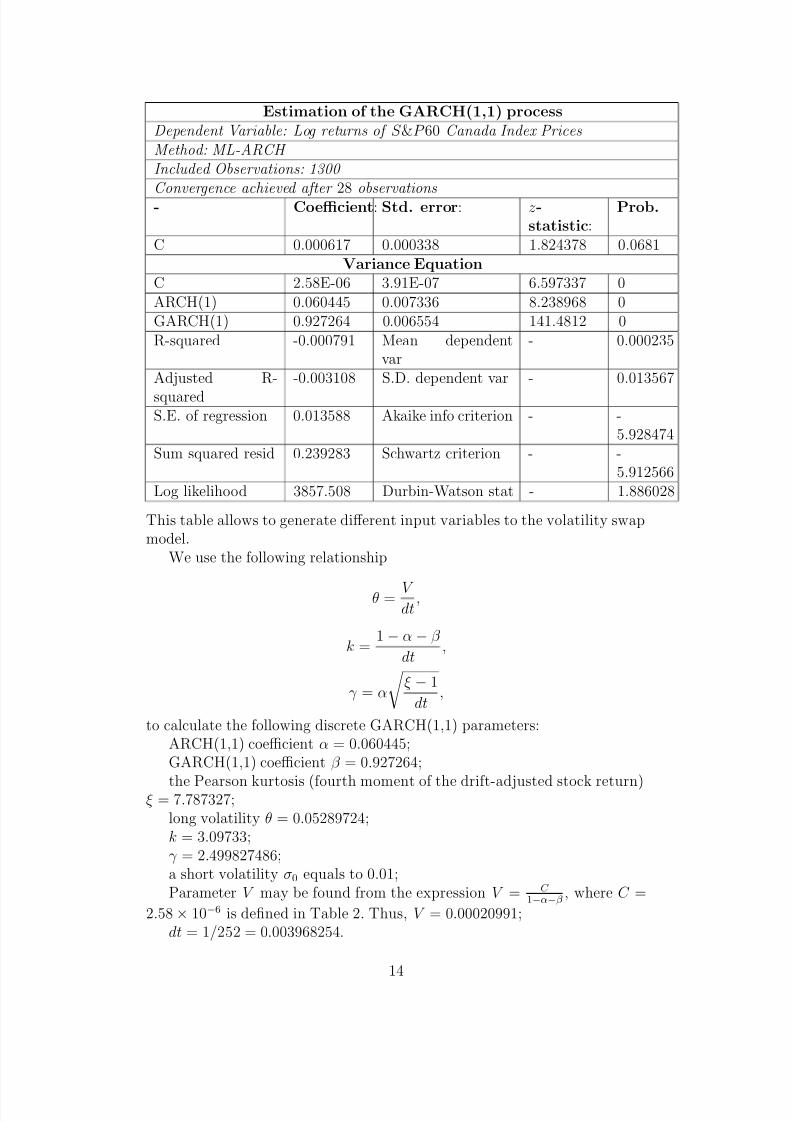
8/6/2019 [York University, Swishchuk Modeling of Variance and Volatility Swaps for Financial Markets With Stochastic Volatility
http://slidepdf.com/reader/full/york-university-swishchuk-modeling-of-variance-and-volatility-swaps-for-financial 14/19
Estimation of the GARCH(1,1) processDependent Variable: Log returns of S &P 60 Canada Index PricesMethod: ML-ARCH Included Observations: 1300
Convergence achieved after 28 observations- Coefficient: Std. error: z-statistic:
Prob.
C 0.000617 0.000338 1.824378 0.0681Variance Equation
C 2.58E-06 3.91E-07 6.597337 0ARCH(1) 0.060445 0.007336 8.238968 0GARCH(1) 0.927264 0.006554 141.4812 0R-squared -0.000791 Mean dependent
var- 0.000235
Adjusted R-
squared
-0.003108 S.D. dependent var - 0.013567
S.E. of regression 0.013588 Akaike info criterion - -5.928474
Sum squared resid 0.239283 Schwartz criterion - -5.912566
Log likelihood 3857.508 Durbin-Watson stat - 1.886028
This table allows to generate different input variables to the volatility swapmodel.
We use the following relationship
θ = V dt
,
k =1 − α − β
dt,
γ = α
ξ − 1
dt,
to calculate the following discrete GARCH(1,1) parameters:ARCH(1,1) coefficient α = 0.060445;GARCH(1,1) coefficient β = 0.927264;
the Pearson kurtosis (fourth moment of the drift-adjusted stock return)ξ = 7.787327;long volatility θ = 0.05289724;k = 3.09733;γ = 2.499827486;a short volatility σ0 equals to 0.01;Parameter V may be found from the expression V = C
1−α−β , where C =
2.58× 10⁻⁶ is defined in Table 2. Thus, V = 0.00020991;dt = 1/252 = 0.003968254.
14
8/6/2019 [York University, Swishchuk Modeling of Variance and Volatility Swaps for Financial Markets With Stochastic Volatility
http://slidepdf.com/reader/full/york-university-swishchuk-modeling-of-variance-and-volatility-swaps-for-financial 15/19
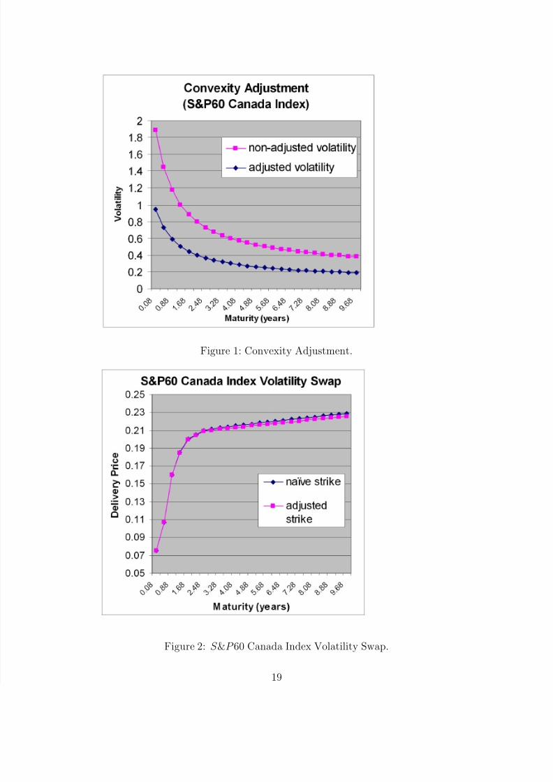
Now, applying the analytical solutions (9) and (13) for a swap maturityT of 0.91 year, we find the following values:
E V =1 − e−kT
kT (σ2
0 − θ2) + θ2 = .3364100835,
and
V ar(V ) = γ 2e−2kT
2k3T 2[(2e2kT − 4ekT kT − 2)(σ2
0 − θ2)+ (2e2kT kT − 3e2kT + 4ekT − 1)θ2] = .0005516049969.
The convexity adjustment V arV
8E V 3/2is equal to .0003533740855.
If the non-adjusted strike is equal to 18.7751%, then the adjusted strikeis equal to
18.7751% − 0.03533740855% = 18.73976259%.
This is the fixed leg of the volatility swap for a maturity T = 0.91.Repeating this approach for a series of maturities up to 10 years we ob-
tain the following plot (see Appendix, Figure 2) of S &P 60 Canada IndexVolatility Swap.
Figure 1 (see Appendix) illustrates the non-adjusted and adjusted volatil-ity for the same series of maturities.
6 Conclusions
In this paper, we presented a new probabilitic approach, based on changingof time method, to study variance and volatility swaps for financial marketswith underlying asset and variance that follow the Heston (1993) model.
We obtained the formulas for variance and volatility swaps which aresimilar to those in the paper by Brockhaus & Long (2000), obtained byanother analytical approach.
We also studied covariance and correlation swaps for the financial marketswith two underlying assets with stochastic volatilities.
As an application of our analytical solutions, we provided a numericalexample using S &P 60 Canada Index to price swap on the volatility.
Acknowledgements. The author thanks to anonymous referee for
valuable suggestions, Paul Wilmott for helpful comments and feedback, andRaymond Theoret (Universite du Quebec a Montreal, Montreal, Quebec,Canada) and Pierre Rostan (Analyst at the R&D Department of Bourse deMontreal and Universite du Quebec a Montreal, Montreal, Quebec, Canada)for S &P 60 Canada Index data. The author remains responsible for any errorsin this paper.
15
8/6/2019 [York University, Swishchuk Modeling of Variance and Volatility Swaps for Financial Markets With Stochastic Volatility
http://slidepdf.com/reader/full/york-university-swishchuk-modeling-of-variance-and-volatility-swaps-for-financial 16/19
7 References.
Avellaneda, M., Levy, A. and Paras, A. (1995): Pricing and hedg-ing derivative securities in markets with uncertain volatility, Appl. Math.Finance 2, 73-88.
Black, F. and Scholes, M. (1973): The pricing of options and corporateliabilities, J. Political Economy 81, 637-54.
Bollerslev, T. (1986): Generalized autoregressive conditional heteroscedas-ticity, J. Economics 31, 307-27.
Brockhaus, O. and Long, D. (2000): ”Volatility swaps made simple”,RISK, January, 92-96.
Buff, R. (2002): Uncertain volatility model. Theory and Applications.NY: Springer.
Carr, P. and Madan, D. (1998): Towards a Theory of Volatility Trading .In the book: Volatility, Risk book publications,http://www.math.nyu.edu/research/carrp/papers/.
Chesney, M. and Scott, L. (1989): Pricing European Currency Op-tions: A comparison of modifeied Black-Scholes model and a random variancemodel, J. Finan. Quantit. Anal. 24, No3, 267-284.
Cox, J., Ingersoll, J. and Ross, S. (1985): ”A theory of the termstructure of interest rates”, Econometrica 53, 385-407.
Demeterfi, K., Derman, E., Kamal, M. and Zou, J. (1999): A guideto volatility and variance swaps, The Journal of Derivatives, Summer, 9-32.
Duan, J. (1995): The GARCH option pricing model, Math. Finance 5,13-32.
Elliott, R. and Swishchuk, A. (2002): Studies of completeness of Brownian and fractional (B,S,X )-securities markets. Working paper.
Frey, R. (1997): Derivative asset analysis in models with level-dependentand stochastic volatility, CWI Quarterly 10, 1-34.
Griego, R. and Swishchuk, A. (2000): Black-Scholes Formula for aMarket in a Markov Environment, Theory Probab. and Mathem. Statit. 62,9-18.
He, R. and Wang, Y. (2002): ”Price Pseudo-Variance, Pseudo Covari-ance, Pseudo-Volatility, and Pseudo-Correlation Swaps-In Analytical CloseForms”, RBC Financial Group, Query Note for 6th ISPW, PIMS, Vancouver,University of British Columbia, May 2002.
16
8/6/2019 [York University, Swishchuk Modeling of Variance and Volatility Swaps for Financial Markets With Stochastic Volatility
http://slidepdf.com/reader/full/york-university-swishchuk-modeling-of-variance-and-volatility-swaps-for-financial 17/19
Heston, S. (1993): ”A closed-form solution for options with stochasticvolatility with applications to bond and currency options, Review of Finan-cial Studies, 6, 327-343
Hobson, D. and Rogers, L. (1998): Complete models with stochastic
volatility, Math. Finance 8, no.1, 27-48.
Hull, J. (2000): Options, futures and other derivatives, Prentice Hall, 4thedition.
Hull, J., and White, A. (1987): The pricing of options on assets withstochastic volatilities, J. Finance 42, 281-300.
Ikeda, N. and Watanabe, S. (1981): Stochastic Differential Equationsand Diffusion Processes, Kodansha Ltd., Tokyo.
Javaheri, A., Wilmott, P. and Haug, E. (2002): GARCH and volatil-
ity swaps, Wilmott Technical Article, January, 17p.
Johnson, H. and Shanno, D. (1987): Option pricing when the varianceis changing, J. Finan. Quantit. Anal. 22,143-151.
Kazmerchuk, Y., Swishchuk, A., Wu, J. (2002): The pricing of op-tions for security markets with delayed response (submitted to MathematicalFinance journal).
Kazmerchuk, Y., Swishchuk, A. and Wu, J. (2002): A continuous-time GARCH model for stochastic volatility with delay, 18p. (Submitted toEuropean Journal of Applied Mathematics).
Merton, R. (1973): Theory of rational option pricing, Bell Journal of Economic Management Science 4, 141-183.
Øksendal, B. (1998): Stochastic Differential Equations: An Introduction with Applications. NY: Springer.
”Price Pseudo-Variance, Pseudo-Covariance, Pseudo-Volatility, and Pseudo-Correlation Swaps-In Analytical Closed-Forms,” Proceedings of the SixthPIMS Industrial Problems Solving Workshop, PIMS IPSW 6, University of British Columbia, Vancouver, Canada, May 27-31, 2002, pp. 45-55. Ed-itor: J. Macki, University of Alberta, June 2002. (So-joint report: Ray-
mond Cheng, Stephen Lawi, Anatoliy Swishchuk, Andrei Bade-scu, Hammouda Ben Mekki, Asrat Fikre Gashaw, Yuanyuan Hua,Marat Molyboga, Tereza Neocleous, Yuri Petrachenko).
Scott, L. (1987): Option pricing when the variance changes randomly:theory, estimation and an application, J. Fin. Quant. Anal. 22, 419-438.
Stein, E. and Stein, J. (1991): Stock price distributions with stochasticvolatility: an analytic approach, Review Finan. Studies 4, 727-752.
17
8/6/2019 [York University, Swishchuk Modeling of Variance and Volatility Swaps for Financial Markets With Stochastic Volatility
http://slidepdf.com/reader/full/york-university-swishchuk-modeling-of-variance-and-volatility-swaps-for-financial 18/19
Swishchuk, A. (1997): Hedging of options under mean-square criterionand with semi-Markov volatility, Ukrain. Math. J. 47, No7, 1119-1127.
Swishchuk, A. (2000): Random Evolutions and Their Applications. New Trends, Kluwer Academic Publishers, Dordrecht, The Netherlands.
Swishchuk, A. and Kalemanova, A. (2000): Stochastic stability of interest rates with jumps. Theory probab. & Mathem statist., TBiMC Sci.Publ., v.61. (Preprint on-line: www.math.yorku.ca/˜aswishch/sample.html )
Theoret, R., Zabre, L. and Rostan, P. (2002): Pricing volatilityswaps: empirical testing with Canadian data. Working paper , Centre deRecherche en Gestion, Document 17-2002, July 2002.
Wiggins, J. (1987): Option values under stochastic volatility: Theory andEmpirical Estimates, J. Finan. Econ. 19, 351-372.
Wilmott, P., Howison, S. and Dewynne, J. (1995): Option Pricing:Mathematical Models and Computations. Oxford: Oxford Financial Press.
8 Appendix: Figures.
18
8/6/2019 [York University, Swishchuk Modeling of Variance and Volatility Swaps for Financial Markets With Stochastic Volatility
http://slidepdf.com/reader/full/york-university-swishchuk-modeling-of-variance-and-volatility-swaps-for-financial 19/19
Figure 1: Convexity Adjustment.
Figure 2: S &P 60 Canada Index Volatility Swap.


![[Dresdner Klein Wort, Bossu] Introduction to Volatility Trading and Variance Swaps](https://static.fdocuments.us/doc/165x107/55017cf54a795974588b4e20/dresdner-klein-wort-bossu-introduction-to-volatility-trading-and-variance-swaps.jpg)

![Nail In The Coffin The Irony in the Variance Swaps...“Variance swaps are ideal instruments to bet on volatility: unlike vanilla op tions, [they] do not require any delta-hedging.”](https://static.fdocuments.us/doc/165x107/61290b8ab1c9ea19794324b3/nail-in-the-coffin-the-irony-in-the-variance-swaps-aoevariance-swaps-are-ideal.jpg)