Ying Li Master of Science In Sociology Dr. Michael Hughes ...

Rural Income and Wealth Inequality in China---

A Study of Anhui and Sichuan Provinces, 1994-1995

Ying Li

Thesis submitted to the Faculty of the Virginia Polytechnic Institute and State

University in partial fulfillment of the requirements for the degree of

Master of Science

In

Sociology

Dr. Michael Hughes, Chair

Dr. Theodore Fuller

Dr. Bradley Hertel

June 12, 2000

Blacksburg, Virginia

Keywords: Rural China, Income Inequality, Wealth Inequality

ii

Rural Income and Wealth Inequality in China---

A Study of Anhui and Sichuan Provinces, 1994-1995

Ying Li

(ABSTRACT)

China has been experiencing a great transition from a socialist collective economy

to a market economy since 1978. Before the transition started, the Communist Party had

established a socialist collective system with very low levels of income and wealth

inequality. With the deepening of the rural reform and the development of rural industry,

a large number of people were lifted out of poverty. However, as the people’s living

standards are rising, disparities in income and wealth are also being accentuated. This

thesis’s main purpose is to study the extent and determinants of income and wealth

inequality in rural China. Based on a sample survey data from Anhui and Sichuan

provinces, the thesis answers the following five questions: 1. How much income and

wealth inequality is there in rural China in 1994-1995? 2. How has inequality in rural

China changed since the reform of 1978? 3. How do the components of income and

wealth in China affect the income and wealth distributions? 4. What social and economic

factors are most responsible for influencing income and wealth in rural China? 5. How

much of the inequality in income and wealth can be accounted for by the factors that

predict income and wealth?

The main findings of the study are, first, rural income inequality was low in the

two provinces in 1994-1995 and wealth inequality was higher than income inequality.

Second, in the industrialized Sichuan province, nonagricultural income made a big

contribution to income inequality, while in the agricultural Anhui province, agricultural

income played an important role in increasing income inequality. Third, education, good

land, sufficient labor, and better communication resources are positively related to

income and wealth.

iii

Acknowledgements

I own my heartfelt thanks to three fabulous members on my thesis’s committee. I

would like to thank my committee chair---Dr. Hughes for his consistent encouragement

and support during my two years’ graduate study at Virginia Tech. Thank you Dr.

Hughes. It is you who guided me from the beginning of my opening the topic for my

thesis until the end. I am not only impressed by your humorous and clear-cut teaching

style, but also by your full-hearted dedication to your profession. Special thanks to you

for your creative idea of analyzing the Gini on regression residuals. I am grateful for your

guidance, suggestions, and patience in helping me finish this biggest project in my

academic life so far.

I thank Dr. Fuller for his precious suggestions and time spent on advising my

thesis as my committee member, and my graduate life as the graduate director. Thank

you Dr. Fuller for your consistent support and help, especially for your insightful ideas on

my methodological analysis and the overall theme and implications of my thesis.

Dr. Hertel is a professor who always likes to explore things into the deepest level

until there is nothing he can do to perfect those things. I am lucky to have him on my

committee. I thank Dr. Hertel for his detailed modifications on my thesis, for his posing

insightful questions to the analysis part of my thesis, and for his taking his precious time

to enrich my extracurricular life by teaching me sledding and a lot of other fun things.

Special thanks to my great Mom for her continuous spiritual support to me and for

my aunt for her consistent support in providing me materials from China.

I would also like to thank my graduate cohorts for being my good friends and

giving me a wonderful graduate life.

iv

Table of Contents

ABSTRACT............................................................................................................... ii

Acknowledgements ................................................................................................... iii

Table of Contents ...................................................................................................... iv

List of Tables.............................................................................................................. v

Chapter 1: Literature Review and Problem Statement............................................... 1

1.1 Introduction .......................................................................................................... 1

1.2 Review of Literature............................................................................................. 3

1.2.1 Historical Background of Rural Reforms in China........................................ 3

1.2.2 Current Studies on Income and Wealth Inequality in Rural China................ 4

1.2.3 Modern Western Theories on Social Stratification ...................................... 10

1.3 Statement of Problem......................................................................................... 11

Chapter 2: Data and Methods................................................................................... 13

2.1 Data Description................................................................................................. 13

2.2 Methodological Issues........................................................................................ 13

2.3 Analysis Process................................................................................................. 14

2.3.1 Four Step Analysis .......................................................................................... 14

2.3.2 Components of Annual Total Income ............................................................. 15

2.3.3 Components of Wealth.................................................................................... 15

2.3.4 Independent Variables in the Regression Analysis ......................................... 16

Chapter 3: Findings .................................................................................................. 18

3.1 Level of Income and Wealth Inequality in Anhui and Sichuan ......................... 18

3.2 Decomposition of Income and Wealth Inequality.............................................. 20

3.3 Income and Wealth Regression Analysis........................................................... 25

3.4 Gini on Regression Residuals ............................................................................ 34

Chapter 4: Conclusions ............................................................................................ 36

4.1 Summary ............................................................................................................ 36

4.2 Discussion and Conclusions............................................................................... 38

4.3 Limitations and Suggestions for Future Research.............................................. 40

Bibliography............................................................................................................. 42

Vita...........................................................................................................................44

v

List of Tables

Table 1 (i). Total Income Ginis for Anhui and Sichuan in 1994 and 1995................. 18

Table 1 (ii). Total Wealth Ginis for Anhui and Sichuan in 1994 and 1995................ 18

Table 2. Rural Gini Coefficients (per capital net income) .......................................... 19

Table 3 (i). Rural Income Inequality and its Sources (Anhui 1994) ........................... 21

Table 3 (ii). Rural Income Inequality and its Sources (Anhui 1995).......................... 21

Table 3 (iii). Rural Income Inequality and its Sources (Sichuan 1994)...................... 22

Table 3 (iv). Rural Income Inequality and its Sources (Sichuan 1995) ...................... 22

Table 4 (i). Rural Wealth Inequality and its Sources (Anhui 1994) ........................... 23

Table 4 (ii). Rural Wealth Inequality and its Sources (Anhui 1995) .......................... 24

Table 4 (iii). Rural Wealth Inequality and its Sources (Sichuan 1994) ...................... 24

Table 4 (iv). Rural Wealth Inequality and its Sources (Sichuan 1995)....................... 24

Table 5 (i). Anhui 1994 Income Regressions.............................................................. 26

Table 5 (ii). Anhui 1995 Income Regressions............................................................. 27

Table 5 (iii). Sichuan 1994 Income Regressions......................................................... 29

Table 5 (iv). Sichuan 1995 Income Regressions......................................................... 30

Table 6 (i). Anhui 1994 Wealth Regressions .............................................................. 31

Table 6 (ii). Anhui 1995 Wealth Regressions ............................................................. 32

Table 6 (iii). Sichuan 1994 Wealth Regressions ......................................................... 33

Table 6 (iv). Sichuan 1995 Wealth Regressions ......................................................... 34

Table 7. Gini for Income Regression Residuals in Comparison with Gini for Total

Income...........................................................................................................35

Table 8. Gini for Wealth Regression Residuals in Comparison with Gini for Total

Wealth ...........................................................................................................35

1

Chapter 1: Literature Review and Problem Statement

1.1 Introduction

The purpose of this study is to investigate the extent and determinants of income

and wealth inequality in rural China in the mid-1990s. Many studies have been done

concerning income and wealth inequalities in western countries. In the US, where income

inequality has been found to be increasing sharply since about 1975 (Gilbert, 1998:20),

there is a more unequal distribution of wealth. This leads to my attention to research into

China’s income and wealth inequality.

As is well known, modern China was founded as a socialist country in 1949. One

thing the government and the Communist Party stressed before reform in 1978 was

equality among all. The commune was the dominant unit of rural economic organization

during that time. Peasants belonging to the same commune worked together and were

paid equally. The Family Production Responsibility System was introduced when the

reform started in 1978 from the countryside. Rural production changed from the

collective level to household level. Individual families were allowed to contract land

from the commune and also allowed to lease land for farm production. The family agreed

to a quota for agricultural produce levied by the collective and could keep the surplus

beyond the quota. Therefore, peasants became more motivated and overall agricultural

production increased rapidly. In addition, before 1979, central planning and government

regulations bound the Chinese peasants tightly to the land, and cultivation, particularly

grain production, had priority over all other activities. Although non-agricultural

activities were not prohibited, they served the function of supporting agriculture by

providing it with modern material inputs. In the early 1980s, the policy toward rural

nonagricultural activities changed and they were regarded as a means of generating

employment opportunities. As the reform deepened and widened, inequality increased

and complaints could be heard about the increasing income gap between rich and poor

even though the overall income level was increasing: rural per capita income increased

from Ren Min Bi (RMB) 134 (about US$ 16) in 1978 to RMB 1926 (about US$ 232) in

1996 (adjusted for inflation to 1996 consumer prices from China Annual Statistics Book,

1997). China’s farmers have gone from the shared poverty to current uneven wealth.

2

China is a big country and consists of provinces that are diverse in terms of land

resources and economic opportunities. So it can provide more detailed contextual

information to focus on specific provinces in studying income and wealth inequality. The

present study focuses on two rural provinces. My initial questions are: How different are

the two provinces studied (Sichuan in the southwest part of China and Anhui in the

southeast part of China) in inequality? To what extent can they represent the whole

picture of rural China? I will then investigate five research questions:

1. How much income and wealth inequality is there in rural China in 1994-1995?

I plan to investigate this by calculating the Gini coefficients for income and

wealth in the two provinces (The Gini index is a measure of inequality

ranging from 0 (absolute equality) to 1 (absolute inequality) with values in

between indicating different levels of inequality).

2. How has inequality in rural China changed since the reform of 1978? I will

investigate this by comparing the Gini coefficients over time.

3. How do the components of income and wealth in China affect the income and

wealth distributions? To answer this question, I will decompose the

differences in Gini coefficients and find out which sources of income and

wealth distributions show the highest levels of inequality and which most

account for the Gini score for the overall income or wealth inequality.

4. What social and economic factors are most responsible for influencing income

and wealth in rural China? I will investigate this by regressing income and

wealth on relevant variables [characteristics of the villages investigated; size

of family; number of laborers in the household; number of staff and workers;

number of children at the age of 15 to 17; number of people working at

township enterprises; number of people going outside the village to work

(A29); level of education of laborers; original value of year-end fixed assets

for production (for income regression analysis only); land, water, and hilly

areas under household’s cultivation]. I expect that each of these factors will

have a positive impact on income and wealth.

5. How much of the inequality in income and wealth can be accounted for by the

factors that predict income and wealth? Will income and wealth inequality be

3

reduced by controlling those factors? I plan to investigate this by calculating

Gini indices on income and wealth regression residuals? I expect that the Gini

on residuals will be reduced proportionally according to how much social and

economic factors can explain income/wealth?

1.2 Review of Literature

1.2.1 Historical Background of Rural Reforms in China

Before 1949, old China had a relatively high level of inequality compared to other

Asian countries. After the Communist Party took control of China in 1949, the

government attached much importance to egalitarianism. The production and distribution

model under Chairman Mao from the 1950s to the mid-1970s depended upon a socialist

collective system for production, capital for growth of output, and a central planning

system for distribution. Considerations of local sufficiency usually exerted influence on

production decisions. In order to produce sufficient supplies of grain and other

agricultural produce, each region channeled its natural, financial and human resources to

agricultural production. Although distribution was based on a work-point allocation

system, it was very egalitarian. Everyone got his/her equal share from the collective “iron

pot”. The administrative structure at that time was ranked down as communes, brigades,

and production teams. Egalitarianism didn’t bring much growth to the rural economy. It

stifled individuals’ initiative for production because rewards were not linked to

performance.

From 1979 to 1984, the first phase of reform focused on decollectivizing

agriculture by introducing the household responsibility system. In terms of administrative

structures, the communes were gradually replaced by township administrations. Land was

allocated to households on a very equal basis and farmers were allowed to keep the rest

of agricultural output after paying the quotas and taxes to the state. The household

responsibility system allowed some farmers to become rich as their efforts were directly

linked to production performance. Grain production and rural incomes increased rapidly

in most regions of the country. The average annual income growth rate during this period

was 12.7 percent (Yao and Zhu, 1998).

4

The second phase of the reform started from 1985 with a changed focus away

from the agricultural sector to the rural industrial sector. The structure of state taxes and

prices was reformed and an attempt was made to build a marketing and trading network.

Efforts were made to develop non-farm enterprises---township and village enterprises

(TVEs). TVEs are owned and operated by villages or townships and financed initially

from surpluses generated within the community. Managers have usually been the

township and village leaders. The new policy was interpreted as “leave the land but not

the countryside; enter the factory but not the city.” Chinese farmers responded to this

policy with great enthusiasm. Therefore farm production slowed down substantially.

Millions of workers were transferred out of agriculture. Between 1978 and 1987, rural

non-agricultural employment increased by 50.3 million---an average rate of 15.5 percent

per year (Ho, 1995). The share of TVE income as a proportion of rural per capita income

grew from 7 percent in 1978 to almost 40 percent in 1992. Although poverty had been

greatly reduced in rural China since reform, increasing disparity in rural income

persisted. Before reform, China was one of the most egalitarian countries in the world.

After two decades of reform, China had moved dramatically toward levels of inequality

of some of its neighboring Asian countries. Based on Yao and Zhu’s paper on inequality

in China (1998), China has the Gini scores of 0.288 and 0.388 for 1981 and 1995

respectively, while South Asia’s Ginis are 0.350 and 0.318, and East Asia have Ginis of

0.387 and 0.381 for the same period.

1.2.2 Current Studies on Income and Wealth Inequality in Rural China

Inequalities of income and wealth are of great social importance because income

and wealth serve the function of providing the basic necessities of life. Income is defined

as “money, wages, and payments that periodically are received as returns from an

occupation or investments” (Kerbo, 1996: 19); and “wealth is accumulated assets in the

form of various types of valued goods, such as real estate, stocks, bonds, or money held

in reserve” (Kerbo, 1996: 19).

5

1.2.2.1 Rural Income Inequality in China

i. Pre-reform period (1949-1978)

Relying on the data on the distribution of collective income in the rural areas of

Hebei and Guangdong provinces, Griffin and Saith (1982) measured rural income

inequality and the determinants of inequality before the decollectivization period of

China began in 1979. They first explained that their data had an upward bias on

inequality because they used collective income and outside employment opportunities

were rationed more favorably for the poorer households. They found out that there was

little inequality in per capita incomes in production brigades and teams and larger

inequality across communes due to the structural factors of the quantity and quality of

land.

ii. First phase of reform (1978-1984) and second phase of reform (1984 and later)

Rozelle (1994) analyzed the data from Jiangsu province during the period of 1984

through 1989 to get the result that evolving patterns of inequality were closely related

with changing economic structures in rural China. In addition to finding a significant

increase in inequality from 1984 to 1989, he found that policies stressing importance of

agriculture reduced inequality while policies promoting rural industry increased it. The

interregional inequality was increasing in large part due to the expansion of rural

industry. Because serious impediments slowed the free flow of products and beneficial

factors such as easy access to resources in rural China, many regions still relied heavily

on local capital and resources to develop. As a result, the rich get richer and the poor get

poorer. So, Rozelle suggested that in order to reduce inequality, policy makers should try

to find ways of breaking the barriers that kept large part of rural society from enjoying

the benefits of the success in the rapidly growing areas.

Drawing on a survey of 10,000 households done by the Chinese Academy of

Social Sciences in 1986, Hussain et al. (1994) confirmed that at that time rural income

inequality in China was very low by international standards [with rural Gini coefficients

ranging from 0.195 (Anhui) to 0.281 (Guangdong)]. Moreover, nonfarming income was

more unevenly distributed than farming income, and the implication was that rural

6

income inequality would rise with a shift in labor from farming activities to nonfarming

activities.

A sample survey was done in 1986 from 249 households in one county in central

Guangdong province. Using the survey data, Hare (1994) computed the Gini index of per

capita total income to be 0.31. Among his findings, non-agricultural income was less

equally distributed than agricultural income. Among non-agricultural income, the

distribution of wage income was more egalitarian than that of self-employment income.

Personal characteristics such as age and marital status were strong determinants of wage

employment. Specifically, young men and young single women were the most likely to

engage in wage employment. Self-employment was strongly related to the household’s

connections and class background, i.e. those who had connections with political

leadership or who were of wealthy class background were more likely to be self-

employed.

Using an alternative data set from a joint survey carried out in the late 1984 and

early 1985 by the Rural Policy Research Unit and the Rural Development Research

Center of the State Council, Bramall and Jones (1993) concluded that there was a sharp

increase in rural income inequality and found that the rural Gini index was around 0.40 in

1984 (1993: 65). They also found out that farm sector income had remained remarkably

equal and non-farm sector incomes were very unequal. They criticized the data collected

by the State Statistical Bureau for its under-representing of the households at the top and

bottom ends of the income scale which would certainly reduce the Gini. They believed

the alternative data set consisted of a broadened income definition and sampled a wider

range of households. Hence they came up with a much higher Gini compared with the

figure of 0.258 obtained by the State Statistical Bureau.

Khan et al. (Griffin and Zhao: 1993) calculated the Gini index to be 0.338 for the

rural China in their research on household income and distribution in China. They carried

out the survey in 1988 investigating 10,258 households in 28 provinces. They found that

income inequality had increased since the early 1980s. However, after comparing their

findings with other developing countries in Asia such as India (the Gini of 0.42 for year

1975/76), Indonesia (the Gini of 0.321 for year 1987), and Philippines (the Gini of 0.43

7

for year 1985), they concluded that the degree of rural income inequality in China was

less than that in many of its developing neighbors.

Khan et al. (Griffin and Zhao: 1993) also derived the following findings from

their research on income inequality in China. Income from family production activities

contributed most to total income and reduced inequality on the income distribution.

Wages were the most important factor in increasing income inequality. The rental value

of owner-occupied housing had an effect of alleviating inequality. The remaining sources

of income such as property income were insignificant and had a disequalizing effect on

income distribution. So, the rich people in rural China obtained a larger proportion of

income from wage employment, nonwage income from enterprises and property income.

They received about average proportion of income from sales of farm and nonfarm

produce and in the form of rental value of housing. They got much less than the average

proportion of income from family production. Finally, they paid much less than the

average rate of net taxes. On the contrary, the poor got a larger part of their income from

family production and used a high proportion of it for self-consumption. They received

little from wage employment, property income, and all other income sources, while

paying a higher than average rate of taxes.

Cheng (1996) used the household survey data collected from five provinces

among grain-producing areas of China covering the period from 1993 to 1995. The 1994

data were used for analysis. They got a Gini index of 0.36 for grain producing areas

which was somewhat higher than the official Gini coefficient of 0.32 for all rural areas in

China.

Khan and Riskin (1998) analyzed the income distribution in China based on a

1995 survey drawn from the national rural and urban household sample surveys. They

found that household production activities still contributed most to total rural income

while its share of total income decreased from 74 percent in 1988 to 56 percent in 1995.

Wages were the second largest component of income and their share among total income

increased sharply from 9 percent to over 22 percent in 1995. They calculated the Gini

coefficient for 1995 to be 0.416. The main income sources for the wealthy were wages,

non-farm entrepreneurship and transfers from the state and collectives, while the main

income sources for the poor were farming and rental value of housing.

8

Ho (1995) in his research on income distribution in China found out that there

was a sharp rise in inter-regional income inequality caused primarily by different regional

growth rates of rural non-agricultural activities. Non-agricultural activities in rural areas

are distributed unevenly because the environment for rural industrialization varies

significantly by region. The regions endowed with better infrastructure, greater resources,

more developed non-agricultural activities, and closer proximity to urban areas will

continue to grow more rapidly than poorly endowed regions and the inter-regional

inequality will increase.

iii. Analysis of the inequality trend

Yao and Zhu (1998) looked at income inequality from a variety of perspectives in

their research based on household survey data by State Statistical Bureau and other

relevant studies. They summarized three main features for income distribution in China.

First, they found that rural per capita incomes quadrupled from 1978 to 1996. However,

overall rural income inequality also increased significantly with this rapid income

growth. The rural Gini index rose from 0.212 in 1978 to 0.32 in 1994. Second, much of

rural income inequality can be indirectly explained by uneven development of township

and village enterprises. The TVEs obtain most development in the eastern regions of

China, moderate development in the central regions, and little development in the western

regions.

The 1997 World Bank report (1997) concluded that the Gini coefficient for

overall inequality increased from 0.288 in 1981 to 0.388 in 1995. Employment and

education were found to be two important factors influencing inequality in rural China.

Increased opportunities for off-farm employment not only boosted income growth but

also contributed to rising inequality. The share of off-farm incomes in total income rose

from 7 percent in 1978 to 33 percent in 1994, as farm incomes fell from 78 percent in

1980 to 60 percent in 1995. By 1990, off-farm employment had become the largest

source of inequality, while transfers and migration opportunities played roles in reducing

inequality. However, only a small portion (20%-30%) of income inequality and one-third

or one half of increases in inequality were accounted for by income determinant

variables. Education explained 2.5 - 3.0 percent of income inequality and 8 percent of the

9

increase in inequality from 1985 to 1990. Among all levels of education, only primary

education reduced inequality and all others increased it. Due to the nearly equal

distribution of land, land ownership had little effect on inequality.

iv. Determinants of Household Income

Using the 1988 survey data referred to before, Khan (Griffin and Zhao: 1993)

analyzed the determinants of rural household income in China. In terms of the

composition of total disposable rural income, 74 percent was obtained from household

production of farm and non-farm goods and services, 10 percent from rental value of

owner-occupied housing, 9 percent from wages, and the remaining 7 percent from

miscellaneous receipts such as private transfers. After regressing different explanatory

variables on total disposable household income, he got the following results. In terms of

different categories of household labor endowment, technical workers contributed most

to household income, followed by ordinary and temporary workers, workers in township

enterprises, cadres, owners/managers of private enterprises, officials and farm workers.

The education index was highly significant. Communist Party membership also had a

highly significant coefficient. Coefficients of fixed productive assets and other assets

were also significant. However, the coefficient of land was not significant. The family

size variable, which was explained to be reflective of dependency ratio, was highly

significant. But the returns to family size were diminishing because one member increase

in family size increased household income by RMB239---31 percent of the per capita

rural household income instead of 100 percent.

1.2.2.2 Rural Wealth Inequality in China

Mckinley (Griffin and Zhao: 1993) analyzed rural wealth inequality in China in

1988. He found that there was a relatively lower wealth inequality in rural China with a

Gini index of 0.311 compared to 0.338 for income inequality. Among the four major

components of wealth, land and fixed productive assets reduce inequality while housing

and financial assets increased inequality. The reason why the Gini for wealth is lower

than the Gini for income is because land is the most important and most equally

distributed component of wealth. Land occupied 58.8 percent of total wealth, leaving the

10

rest three components of wealth taking only less than 50 percent. Since land is equally

distributed in China, it has the effect of reducing the total wealth inequality. However in

other developing countries, a large proportion of rural households are landless or nearly

landless and have very few other assets, which results in a higher wealth inequality than

income inequality.

1.2.3 Modern Western Theories on Social Stratification

1.2.3.1 Functional Theories of Social Stratification

Two dominant modern functional theories of social stratification are Davis and

Moore theory, and Parsons theory. The Davis and Moore theory argues that social

stratification and inequality serve the purpose of meeting the needs of complex social

systems. “Among the needs is for the most important positions or jobs in the society to be

staffed by the most qualified and competent people” (Kerbo,1996: 119). Therefore,

social inequality is believed to be positively functional and inevitable in any society.

Parsons’ theory of social stratification argues, “the common value system helps ensure

that the functionally most important roles are filled by competent people through their

status striving” (Kerbo, 1996:123). According to Parsons, people who best live up to the

ideas or values that are given primary stress in the society will receive high income and

wealth.

On the individual level, dimensions of functional theory are things like human

capital and productivity. If a person has more human capital and more resources to

improve productivity, his/her work can be more important and can contribute more to

society. Hence, according to functional theory, he/she should make more money and

inequality will appear.

1.2.3.2 Conflict Theory of Social Stratification

Ralf Dahrendorf is one of the most influential conflict theorists of social

stratification. He incorporates the strong points of both Marx and Weber in his theory.

According to him, societies must be viewed from the perspective of conflict and differing

interests. Power or party acts as the main dimension of social stratification. And political

power or formalized bureaucratic power and authority are often used to explain social

11

inequality and stratification in industrial societies. “The haves get what they want

because they are on top in the social organization, while the have-nots find it in their

interests to challenge the status quo that assign them low positions and low rewards”

(Kerbo, 1996:140).

The major difference between conflict theory and functional theory is that conflict

theory focuses on power while functional theory focuses on ability and productivity. For

conflict theorists, a person has more human capital and more resources because the

person has more power to help him/her get more. So income and wealth is connected to

power. Inequality exists because people in power positions can get the society to work for

them. Therefore, they receive higher incomes and accumulate greater wealth.

1.3 Statement of Problem

A common view can be derived from the above literature on China that income

inequality in rural China has been increasing since 1978, although various studies result

in different Gini coefficients based on different data sets. The major reason for the

increased inequality is the rapid and uneven growth of rural industry, especially township

and village enterprises. One explanation for the uneven development of rural industry is

that regions are unequally endowed in terms of resources (e.g. infrastructure), location

(e.g. closer proximity to urban areas) and regional characteristics (e.g. development of

rural industry).

Pervasively confirmed by various studies on rural China is the fact that non-

agricultural income is more unequally distributed than agricultural income. In terms of

rural income composition, income from family production contributes most to total

income although its share is decreasing; wages rank second and its share is increasing;

rental value of housing takes the third position regarding its contribution to income.

After comparing the two provinces with each other and with other provinces in

China, I will investigate to what extent the two provinces can represent the whole picture

of China. I will compute the Gini coefficients for each province in both 1994 and 1995.

Through comparing these Ginis and those from the literature, I will be able to analyze the

trend of income and wealth inequality in both provinces.

12

Second, I will investigate what effect each source of income/wealth has on

income/wealth inequality. I will decompose the Gini index into sources of income/wealth

to find the result. Those sources which have a higher concentration ratio than the overall

Gini will increase inequality more than sources with lower Gini index scores.

Third, I will do a regression analysis to find out what variables are statistically

significant in determining income and wealth and how much they account for income and

wealth. The variables I will use include family size, number of laborers in the household,

number of children at the age of 15 to 17 in the household, characteristics of the village

investigated, the number of workers in state owned enterprises, township and village

enterprises, and other towns, education, value of productive fixed assets (for income

regression analysis only), and various kinds of cultivation area.

Fourth, I will investigate how my income/wealth determinant variables have an

effect on impacting inequality. I will calculate Gini coefficients on income/wealth

regression residuals and see if the Gini indices will be reduced after taking into account

those variables.

Due to the fact that current studies on income and wealth inequality in rural China

haven’t really provided any theoretical explanations of the issue, my study will try to

develop some theory of social stratification on rural China. Based on the previous

discussion of western theories of social stratification, my analysis will explore the

following three possibilities.

If the functional theory is true, factors such as education and resources (e.g. labor,

land) will explain all the inequality. If conflict theory is true, the previous factors will

explain none of the inequality. If those factors explain some portion of inequality, it

means either some conflict processes may be operating, or not every social functional

process is adequately measured, or luck may be one important element to explain

inequality.

13

Chapter 2: Data and Methods

2.1 Data Description

The data were collected by a rural survey group of the Chinese State Statistical

Bureau in 1994 and 1995 in the two provinces Anhui and Sichuan. Altogether 28

counties, 280 administrative villages, and 2820 households (1820 in Sichuan and 1000 in

Anhui) were surveyed. All counties in each province were ranked by either income per

capita or grain output per Mu (1 Mu = 1/6 acre). A subset of counties was selected based

on a systematic sampling method. A similar sampling method was used to select villages

in each selected county and rural households in each selected village. The household is

the basic income recipient. Household income is measured by the earnings of each

individual member as well as the collective earnings of the household. The annual total

income of the household is composed of basic income (income from payments and

family business), transferred income, and property income.

Anhui is among one of China’s smallest provinces with a population of 57.6

million and an area of 139,400 km2. It has China’s seasonal monsoon climate. The

predominant winter crop is wheat, and summer crops include rice, soybeans, sweet

potatoes and other agricultural products. Its main commercial crops are vegetable

oilseeds, cotton, fibers, and tobacco. Fish farming is common along the Yangtze River.

Anhui possesses abundant agricultural resources and products, occupying 427 million

acres of farmland, 414 million acres of forestland, and 53 million acres of aquatic farm.

Sichuan, situated in the southwest part of China, covers 570,000 km2 and has a

population of 110.84 million. It is among one of the biggest provinces in China. Its land

can be divided into plain, hill, plateau, swamp, forest and grassland with all types of

climate. Sichuan has a long history of developed agriculture and is the biggest producer

of grain in China. The economic development of the province is also stimulated by the

fast growing township and village enterprises.

2.2 Methodological Issues

Various methods exist for measuring inequality. There are simple methods such

as distribution among population tenths and ratios of average incomes of different decile

14

groups. In addition to them, the most popular four among the others are the Gini index,

Squared Coefficient of Variation, Theil’s index, and Variance of Logarithms. The Gini

index is based on the Lorenz curve plotting the share of population against the share of

income or wealth. I have chosen to use that method due to the following reasons. First,

most of the previous inequality studies done in China and in other countries employed

this method. So it is convenient for comparison purposes to use this method in my

research. Second, the Gini index is good at measuring inequality of a less extreme form,

as is the case with inequality in China. Third, the Gini index enables us to decompose

overall inequality into its constitutive sources. This can be demonstrated by the formula

(Griffin and Zhao, 1993:37):

G = ��(Ui * Ci) where

G: the Gini index of total income/wealth

Ui: the share of ith source of income/wealth.

Ci: the concentration ratio of the ith source of income/wealth, i.e. the Gini index

within the ith source of income/wealth.

In this formula, the Gini index is actually the weighted average of the

concentration ratios of various sources of income/wealth, the weights being the shares of

these sources in total income/wealth. If the concentration ratio is higher (lower) than the

overall Gini index, a rise in the share of the corresponding source of income/wealth will

increase (reduce) the overall Gini ratio.

2.3 Analysis Process

2.3.1 Four Step Analysis

The first step in my analysis is to compute the overall Gini index for both income

and wealth for the two provinces in 1994 and 1995.

The second step is to decompose the overall income/wealth inequality into its

component sources and try to find out what share each source occupies in terms of

overall income/wealth, what increasing or decreasing effect on inequality each source

has, and the contribution of each source to overall inequality.

The third step in my analysis is to run income and wealth regressions and

investigate how the selected independent variables affect income/wealth.

15

The fourth step is to calculate the Gini index for income and wealth regression

residuals. Because residuals are variability not explained by my independent variables,

the Gini on residuals will show the inequality left over after independent variables

explain everything they can. In that way, I can see how the independent variables affect

levels of inequality.

2.3.2 Components of Annual Total Income

The components of annual total income are as follows:

(i) Income from payment (wages and salary), including payment from

collective organizations and enterprises, payment from individual, private,

and township and village enterprises, and payment from other work units.

(ii) Income from family business, including income from family-run

agricultural businesses and nonagricultural businesses. Income from

agricultural businesses is composed of income from planting, forestry,

stock raising, fishery, and hunting. Income from nonagricultural

businesses is composed of income from handicraft industry, industry,

construction industry, transport industry, commerce, catering trade,

service industry, and other family businesses.

(iii) Income from transfers, including welfare and relief payments, various

subsidies, pensions, remittances from relatives and friends, rewards,

compensations, and other transfers.

(iv) Income from property , including interest income, rent income, and other

property income.

2.3.3 Components of Wealth

The components of wealth are as follows:

(i) Original value of fixed productive assets

(ii) Year-end value of houses

(iii) Ending cash balance

(iv) Ending savings balance

I haven’t added land value to the total wealth, because land is not individually

16

owned and the data available does not provide enough information to calculate the value

of land.

2.3.4 Independent Variables in the Regression Analysis

The independent variables in my regression analysis are grouped into four

sections. The first section is Education, consisting of five educational indices: primary

school, middle school, high school, technical school, college and higher education. These

indices are constructed by dividing the number of people in each category of education

by the number of laborers in the household. The second group of predictor variables is

Family Structure. This group is composed of six different variables: family size

(number of people in the household), number of laborers, children at 15-17 (number of

children 15 to 17 years old), staff and workers (number of people working for the

government or collective organizations and enterprises), workers in TVEs (number of

people working at township and village enterprises), workers going outside the village

(number of people going outside the village to work). The third group of the independent

variables is Resource Factors. It includes land area (the area of farmland occupied by

the household), hilly area (area of hills occupied by the household), water area ( area of

water occupied by the household), and original value of fixed productive assets. The unit

used to measure the area is Chinese Mu (1 Mu = 1/6 acre). The last group is Context

variables. It has nine variables listed as follows:

� plain (whether the place where the household lives is flat)

� hills (whether the place where the household lives is hilly)

� phone (whether the household has phone at home: 1 is Yes and 0 is No)

� highway (whether there is highway in the village where the household lives: 1

is Yes and 0 is No)

� school (whether there is school in the village where the household live: 1 is

Yes and 0 is No)

� clinic (whether there is clinic in the village where the household lives: 1 is

Yes and 0 is No)

17

� old liberated area (whether the place where the household lives is an area

which was among the first few liberated by the Communist Party during the

civil war in the 1940s: 1 is Yes and 0 is No)

� post office (whether there is a post office in the village where the household

lives: 1 is Yes and 0 is No)

� radio (whether there are radio programs in the village where the household

lives: 1 is Yes and 0 is No).

18

Chapter 3: Findings

3.1 Level of Income and Wealth Inequality in Anhui and Sichuan

From Table 1-(i), we can see that income Ginis for both provinces decreased

slightly from 1994 to 1995. In Anhui, the Gini index was 0.234 in 1994 and 0.229 in

1995, while in Sichuan the income Gini was 0.236 in 1994 and 0.233 in 1995. The

decrease in Gini in Anhui province may be explained by the increase in the share of wage

income and the decrease in the share of property income, because wage income has an

effect of reducing inequality and property income has an effect of increasing inequality.

The slight decrease in Gini in Sichuan province may be attributed to the increase in the

share of agricultural income and the decrease in the share of nonagricultural income in

total income.

The wealth inequality shown in Table 1-(ii) is much higher than the income

inequality. In Anhui, the wealth Gini increased from 0.346 in 1994 to 0.349 in 1995, and

in Sichuan, it increased sharply from 0.368 in 1994 to 0.385 in 1995. One study (Griffin

and Zhao: 1993) discussed in the literature review arrived at a lower wealth inequality

than income inequality because land was included as a component of wealth. The wealth

in my study does not include land for the reason that land is not individually owned, so

the wealth inequality resulting from my study is higher than the income inequality.

Table 1-(i). Total INCOME Ginis for Anhui and Sichuan in 1994 and 1995

Anhui Sichuan

1994 0.234 0.236

1995 0.229 0.233

Table 1-(ii). Total WEALTH Ginis for Anhui and Sichuan in 1994 and 1995

Anhui Sichuan

1994 0.346 0.368

1995 0.349 0.385

From the literature I have reviewed, some results can be pulled out for a

comparison with 1994-1995 income Ginis in the two provinces. These comparisons can

be made by using the following table of overtime Ginis for rural per capita net income in

19

China. The data were based on annual household survey done by the State Statistical

Bureau.

Table 2. Rural Gini Coefficients (per capita net income)

Year Gini Households surveyed

1978 0.212 6,095

1980 0.237 15,914

1986 0.280 66,836

1987 0.300 66,912

1988 0.300 67,186

1989 0.316 66,906

1990 0.315 66,478

1991 0.310 67,410

Sources: State Statistical Bureau, China, 1978-1991

We can see a generally increasing trend of Gini coefficients from the above table.

The paper of Yao and Zhu (1998) provided some data on inequality in the 1990s in other

countries: the Gini score of 0.380 for Middle East and North Africa, 0.493 for Latin

America and the Caribbean, 0.381 for East Asia and the Pacific, 0.318 for South Asia,

0.338 for high-income countries, 0.289 for Eastern Europe. By comparing the Ginis in

the table with those of other countries, we can see that China is having a moderate level

of inequality.

Using a 1986 income inequality study of 10,000 households in China, Hussain et

al. (1994) calculated the Gini index of 0.195 for Anhui and 0.228 for Sichuan. From

Table 2, we know that 1986 Gini was 0.288 for the whole China. Hence, due to the fact

that a large proportion of rural income inequality in China comes from inter-provincial

inequality (Yao and Zhu, 1998:140), the provincial level Gini indices cannot represent

the overall inequality for China. Because Anhui and Sichuan are two provinces with low

income inequality, it is reasonable to predict that the Gini coefficient for all of rural

China in 1994 and 1995 will be much higher than those shown in Table 1.

20

3.2 Decomposition of Income and Wealth Inequality

3.2.1 Income Inequality Decomposition

The four parts of Table 3 present the decomposition of income inequality. As

shown in the table, agricultural income takes up a predominant proportion of the total

income in both provinces. Ranking the second is wage income (except for the case of

1994 Sichuan in which wage income ranks the third), but far behind the share of

agricultural income. Income from nonagricultural activities ranks the third in terms of its

share in total income, followed by transfer income and property income. Looking at the

concentration ratios, I find that in both provinces, transfer income and property income

have a disequalizing effect on overall income distribution. However, due to their small

proportions in total income, their contributions to overall inequality remain small. Wage

income in both provinces has the effect of decreasing overall inequality, which is the

opposite of the patterns in earlier research (Khan et al., 1993). However, the proportion of

wage income in total income increased from 1994 to 1995 in both provinces and its

contribution to overall income inequality increased as well. This may indicate a trend

toward what was described in the literature, i.e., wage income will become an important

component of total income and a disequalizing factor for income inequality.

For the Anhui province, the concentration ratio for income from agricultural

activities is a little higher than the overall Gini index, while the concentration ratio for

nonagricultural income is much lower than the overall Gini. However, the opposite

situation is found in Sichuan province, where nonagricultural income has the effect of

increasing income inequality and agricultural income has the effect of reducing it. I think

the different effects of agricultural income and nonagricultural income in the two

provinces can be explained by the different levels of industrial development in these

provinces: Sichuan is a well-developed industrial base, while Anhui is a relatively

agriculture dominant province. Consequently, nonagricultural income is more important

in Sichuan whereas agricultural income matters more in Anhui.

The income profiles of rich and poor people in Anhui and Sichuan provinces are.

In Anhui, the rich people get a higher than average proportion of income from

agricultural activities, transfers, and property income, while they receive a lower than

average proportion of income from wages and non-agricultural activities. This can be a

21

typical profile of a middle-to-lower level income province where agricultural activities

dominate other types of production and income engendering activities. In Sichuan, the

picture is different. The rich people there get a higher than average proportion of income

from nonagricultural activities, transfers and property income. They receive a close to

average proportion of income from agricultural activities, and a lower than average

proportion of income from wages. In this highly developed industrial province,

nonagricultural activities play a very important role in increasing the gap between the

rich and the poor.

Table 3-(i). Rural INCOME inequality and its sources (ANHUI 1994)

Income and itsComponents

Share of Total Income(%)

Gini or ConcentrationRatio

Contribution ofIncome Component toOverall Inequality (%)

Income from payment

(wages)

8.97 0.178 6.81

Income from

agricultural activities

80.41 0.245 84.24

Income from non-


6.48 0.148 4.11

Income from transfers 1.91 0.255 2.08

Property income 2.22 0.291 2.76

Total Income 100.00 0.234 100.00

Table 3-(ii). Rural INCOME inequality and its sources (ANHUI 1995)





Income from payment

(wages)

9.56 0.182 7.61

Income from


81.22 0.241 85.48

Income from non-


5.64 0.110 2.71



Total Income 100.00 0.229 100.00

22

Table 3-(iii). Rural INCOME inequality and its sources (SICHUAN 1994)





Income from payment

(wages)

8.79 0.199 7.41

Income from


77.30 0.216 70.95

Income from non-


9.01 0.399 15.25



Total Income 100.00 0.236 100.00

Table 3-(iv). Rural INCOME inequality and its sources (SICHUAN 1995)





Income from

payment(wages)

10.12 0.198 8.59

Income from


76.46 0.223 73.33

Income from non-


8.20 0.343 12.06



Total Income 100.00 0.233 100.00

Note: For the above four parts of table 3 (1) Column I is 100 Ui. (2) Column II is the index of inequality,

i.e. the Gini ratio for total income and the concentration ratios for income components. (3) Column III is

100(UiCi)/G.

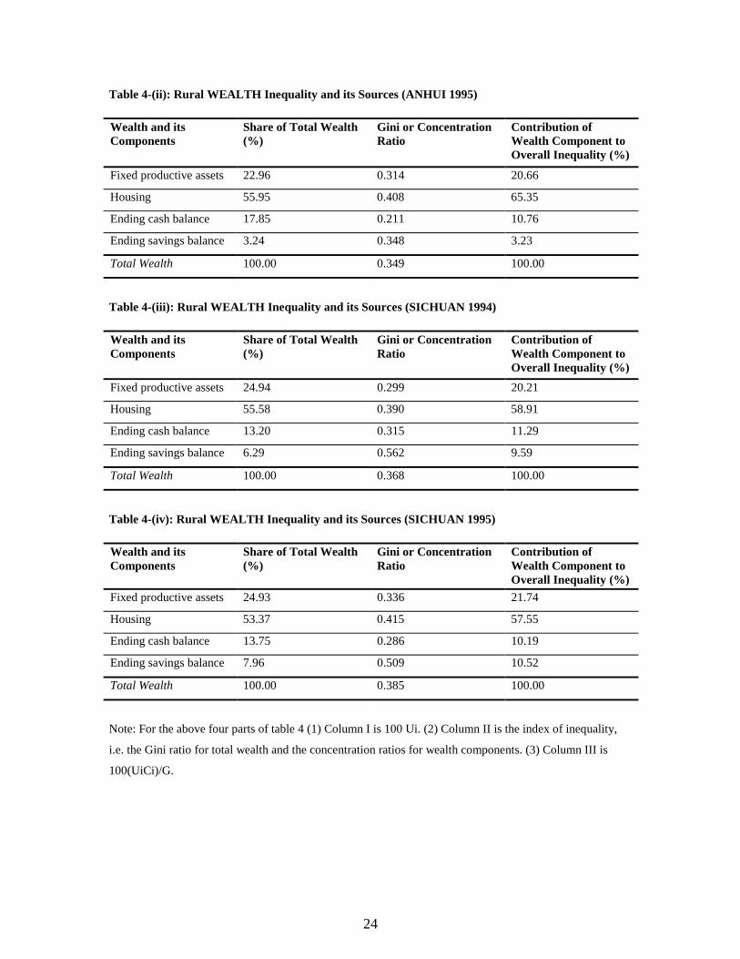
3.2.2 Wealth Inequality Decomposition

From the decomposition of wealth inequality in Table 4, we can see that in both

provinces, housing value occupies more than half of total wealth and also makes the

23

largest contribution to wealth inequality. That is very understandable because farmers in

China give their first priority to build new houses or improve existing houses when their

income increases. It is still many Chinese’s belief that stocks and bonds have some

degree of risk taking and uncertainty. Housing is attractive as a less risky form of

accumulating wealth. However, there has been no real market for houses in rural China,

for farmers build houses on their own with the help of their friends and relatives; also,

almost all housing is private and for self-use.

Original value of fixed productive assets ranks second in terms of its proportion in

overall wealth, followed by ending cash balance and ending savings balance. In Anhui

province, except housing, all other components of wealth have a reducing effect on

wealth inequality. In Sichuan province, ending savings balance has a concentration ratio

much higher than the overall Gini and hence accentuates wealth inequality. Original

value of fixed productive assets and ending cash balance all have the effect of reducing

wealth inequality due to their lower concentration ratios.

In both provinces, we see a trend of increasing share of ending savings balance in

total wealth, accompanied consistently by an increased contribution of ending savings

balance to total wealth inequality. In Anhui where this phenomenon is sharper, the

proportion of ending savings balance in total wealth increased from 2.24 percent to 3.24

percent, a 45 percent increase from 1994 to 1995 while the contribution of ending savings

balance to overall wealth inequality increased 52 percent. This finding may suggest that

saving money in the bank is becoming a new way of accumulating wealth and possibly a

new factor of increasing inequality.

Table 4-(i): Rural WEALTH Inequality and its Sources (ANHUI 1994)

Wealth and itsComponents

Share of Total Wealth(%)


Contribution ofWealth Component toOverall Inequality (%)

Fixed productive assets 21.98 0.287 18.20

Housing 60.39 0.396 69.12

Ending cash balance 15.39 0.237 10.55

Ending savings balance 2.24 0.329 2.13

Total Wealth 100.00 0.346 100.00

24

Table 4-(ii): Rural WEALTH Inequality and its Sources (ANHUI 1995)






Housing 55.95 0.408 65.35



Total Wealth 100.00 0.349 100.00

Table 4-(iii): Rural WEALTH Inequality and its Sources (SICHUAN 1994)






Housing 55.58 0.390 58.91



Total Wealth 100.00 0.368 100.00

Table 4-(iv): Rural WEALTH Inequality and its Sources (SICHUAN 1995)






Housing 53.37 0.415 57.55



Total Wealth 100.00 0.385 100.00

Note: For the above four parts of table 4 (1) Column I is 100 Ui. (2) Column II is the index of inequality,

i.e. the Gini ratio for total wealth and the concentration ratios for wealth components. (3) Column III is

100(UiCi)/G.

25

3.3 Income and Wealth Regression Analysis

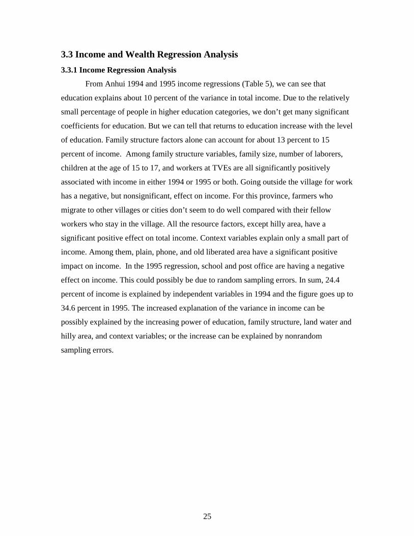
3.3.1 Income Regression Analysis

From Anhui 1994 and 1995 income regressions (Table 5), we can see that

education explains about 10 percent of the variance in total income. Due to the relatively

small percentage of people in higher education categories, we don’t get many significant

coefficients for education. But we can tell that returns to education increase with the level

of education. Family structure factors alone can account for about 13 percent to 15

percent of income. Among family structure variables, family size, number of laborers,

children at the age of 15 to 17, and workers at TVEs are all significantly positively

associated with income in either 1994 or 1995 or both. Going outside the village for work

has a negative, but nonsignificant, effect on income. For this province, farmers who

migrate to other villages or cities don’t seem to do well compared with their fellow

workers who stay in the village. All the resource factors, except hilly area, have a

significant positive effect on total income. Context variables explain only a small part of

income. Among them, plain, phone, and old liberated area have a significant positive

impact on income. In the 1995 regression, school and post office are having a negative

effect on income. This could possibly be due to random sampling errors. In sum, 24.4

percent of income is explained by independent variables in 1994 and the figure goes up to

34.6 percent in 1995. The increased explanation of the variance in income can be

possibly explained by the increasing power of education, family structure, land water and

hilly area, and context variables; or the increase can be explained by nonrandom

sampling errors.

26

Table 5-(i). ANHUI 1994 INCOME regressions

Model 1 Model 2 Model 3 Model 4 Model 5 Model 6EducationPrimary school -396.39 -247.93Middle school 441.79 693.92High school 2384.73* 1967.77*Technical school 3085.69 2666.01College and higher education 3672.83 4522.92

Family StructureFamily size 707.68* 221.25Number of laborers 606.45* 507.60*Children at 15-17 1048.86* 1156.36*Staff and workers 735.00 455.38Workers at TVEs 932.82* 1155.35*Workers going outside thevillage

-644.15* -497.38

Resource factors Land, Water, Hilly Area Land area 3.35* 2.04* Hilly area -0.11* -0.09 Water area 6.31* 4.69* Fixed productive assets 0.50* 0.31*

Context Variablesplain 501.79 -621.28hills 580.12 -710.83phone -246.30 119.40highway -313.56 7.38school 460.51 -506.44clinic 492.26 788.65*Old liberated area 1175.81* 1665.34*Post office -72.77 -42.89radio 125.10 153.37

R2 0.101* 0.132* 0.125* 0.101* 0.016 0.244** P<0.05

27

Table 5-(ii). ANHUI 1995 INCOME regressions

Model 1 Model 2 Model 3 Model 4 Model 5 Model 6EducationPrimary school -563.18 232.09Middle school 1015.94 1009.07High school 2183.95* 1726.08*Technical school 3857.79 3298.01College and higher education 7078.61 8684.89*

Family StructureFamily size 999.92* 452.60*Number of laborers 456.74* 408.29*Children at 15-17 263.42 385.13Staff and workers 1236.75* 869.94Workers at TVEs 295.43 608.23Workers going outside thevillage

-377.49 -53.97


Context Variablesplain 2374.42* 1039.04*hills 1840.25* 143.80phone 274.01 593.01*highway 695.59 448.93school -1494.50* -1439.42*clinic 458.58 235.57Old liberated area 693.41 1332.37*Post office -1157.57* -863.89*radio -351.79 -912.06

R2 0.117* 0.156* 0.193* 0.106* 0.070* 0.346** P<0.05

In Sichuan, education alone explains slightly less than 10 percent of total income.

All indices of education have a positive effect on income although only high school is

significant in both years. The reason why technical school, and college and higher

education indices don’t have a significant impact is because that they don’t have large

enough sample size. We also see from Table 5-(iii and iv) that returns to education

increase with the level of education except technical school index. Its contribution to

income is less than middle school and high school education.

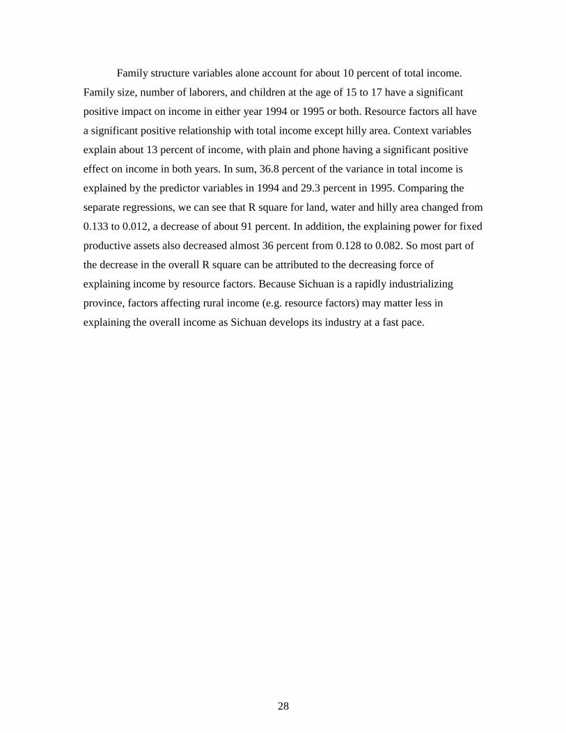
28

Family structure variables alone account for about 10 percent of total income.

Family size, number of laborers, and children at the age of 15 to 17 have a significant

positive impact on income in either year 1994 or 1995 or both. Resource factors all have

a significant positive relationship with total income except hilly area. Context variables

explain about 13 percent of income, with plain and phone having a significant positive

effect on income in both years. In sum, 36.8 percent of the variance in total income is

explained by the predictor variables in 1994 and 29.3 percent in 1995. Comparing the

separate regressions, we can see that R square for land, water and hilly area changed from

0.133 to 0.012, a decrease of about 91 percent. In addition, the explaining power for fixed

productive assets also decreased almost 36 percent from 0.128 to 0.082. So most part of

the decrease in the overall R square can be attributed to the decreasing force of

explaining income by resource factors. Because Sichuan is a rapidly industrializing

province, factors affecting rural income (e.g. resource factors) may matter less in

explaining the overall income as Sichuan develops its industry at a fast pace.

29

Table 5-(iii). SICHUAN 1994 INCOME regressions

Model 1 Model 2 Model 3 Model 4 Model 5 Model 6EducationPrimary school 896.98* 425.37Middle school 1618.50* 667.59*High school 2083.28* 1289.54*Technical school 933.97 693.68College and higher education 2067.08 2701.66

Family StructureFamily size 460.22* 449.52*Number of laborers 439.23* 186.38*Children at 15-17 411.19* 400.89*Staff and workers 250.39 248.51Workers at TVEs 836.75* 322.87Workers going outside thevillage

-94.18 157.19


Context Variablesplain 2463.31* 2083.35*hills 157.07 87.49phone 1125.36* 1307.27*highway -58.13 -386.62school -285.90 -350.29*clinic -86.23 -181.14Old liberated area -310.53* -220.09Post office -267.90 -304.71*radio 896.26* 1233.41*

R2 0.097* 0.108* 0.133* 0.128* 0.124* 0.368** P<0.05

30

Table 5-(iv). SICHUAN 1995 INCOME regressions

Model 1 Model 2 Model 3 Model 4 Model 5 Model 6EducationPrimary school 671.16* 179.22Middle school 1431.18* 427.32High school 1883.87* 1078.22*Technical school 1266.91 377.10College and higher education 4557.85 4158.20

Family StructureFamily size 525.08* 595.40*Number of laborers 564.52* 362.43*Children at 15-17 232.83 290.25Staff and workers 556.42 356.44Workers at TVEs 524.41 75.17Workers going outside thevillage

-493.64* -157.76

Resource factors Land, Water, Hilly Area Land area 0.07* 0.06* Hilly area -0.02 0.01 Water area 6.17* 3.37* Fixed productive assets 0.36* 0.27*

Context Variablesplain 2988.09* 3163.24*hills 319.34 569.65*phone 583.05* 751.84*highway 438.30 576.26*school -167.23 -152.16clinic 449.55* 185.33Old liberated area -765.53* -616.51*

R2 0.087* 0.105* 0.012* 0.082* 0.133* 0.293** P<0.05Note: No post office and radio variables exist in this year of the data.

3.3.2 Wealth Regression Analysis

Looking at wealth regressions for Anhui province, we see that 23.8 percent of the

variance in total wealth is explained by the independent variables in 1994 and only 17.6

percent in 1995. Education explains about 9 percent of the variance in total wealth. Only

high school has a significant positive impact on total wealth. Family structure variables

account for about 10 percent of wealth with family size, number of laborers, and workers

at TVEs having a significant positive effect in both years. Area of farmland owned by the

household also significantly increases wealth. Context variables explain less than 10

31

percent of wealth with phone, highway, clinic, and school having a significant positive

impact on wealth in either 1994 or 1995 or both. The overall R square decreased about

one-fourth from 0.238 to 0.176 in Anhui province. This can be explained by the declining

explanatory ability in resource factors and family structure.

Table 6-(i). ANHUI 1994 WEALTH regressions

Model 1 Model 2 Model 3 Model 4 Model 5EducationPrimary school -106.67 181.88Middle school 1898.24 1449.16High school 3758.88* 2921.26*Technical school 5362.62 3100.31College and higher education 4488.22 5918.41

Family StructureFamily size 1193.88* 606.62*Number of laborers 858.13* 706.48*Children at 15-17 1313.90* 1105.62Staff and workers 1534.40 1119.01Workers at TVEs 4473.45* 3907.12*Workers going outside thevillage

-771.69 -151.04

Resource Factor Land, Water, Hilly Area Land area 5.05* 5.24* Hilly area -0.08 -0.23 Water area 5.56* 2.46

Context Variablesplain 2690.47* 1227.88hills 106.34 -2523.61*phone 2072.00* 2420.52*highway -1608.58* -763.42school 4291.74* 3079.48*clinic -1171.93 -948.69Old liberated area -884.00 -515.89Post office -986.08 -1028.47radio -362.50 -308.38

R2 0.086* 0.135* 0.089* 0.044* 0.238** P<0.05

32

Table 6-(ii). ANHUI 1995 WEALTH regressions

Model 1 Model 2 Model 3 Model 4 Model 5EducationPrimary school -453.27 -653.45Middle school 3371.36* 2443.45High school 6822.90* 5807.55*Technical school -1521.60 -3873.97College and higher education -5566.52 -4726.87

Family StructureFamily size 1448.42* 1098.32*Number of laborers 845.02* 1018.04*Children at 15-17 -206.01 322.36Staff and workers -316.03 -717.64Workers at TVEs 4116.50* 3459.77*Workers going outside thevillage

-467.16 -424.59

Resource Factor Land, Water, Hilly Area Land area 2.75* 2.11* Hilly area 0.09 0.01 Water area 4.42 1.12

Context Variablesplain 2748.92* 1446.71hills 343.11 -1215.33phone 1171.50 1078.17highway 4179.91* 4083.93*school 3856.45* 4054.68*clinic -2913.43* -3183.60*Old liberated area -1392.11 -626.52Post office 634.02 726.24radio 284.50 -374.65

R2 0.080* 0.093* 0.024* 0.058* 0.176** P<0.05

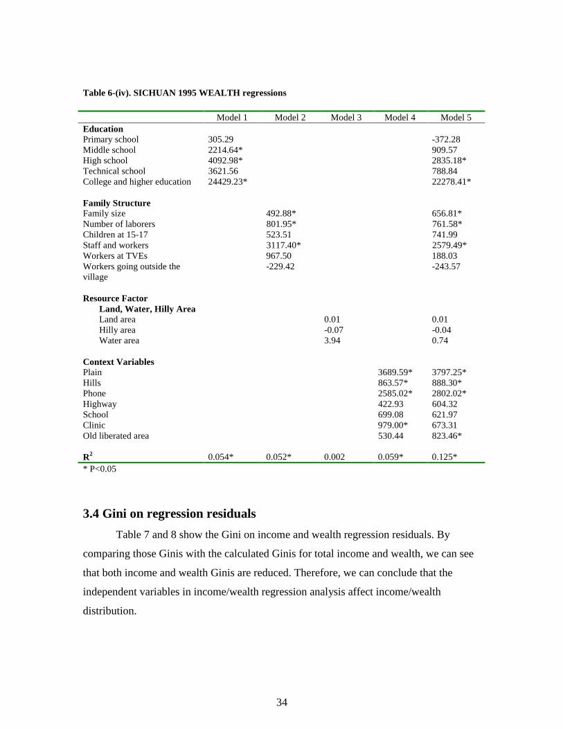
The wealth regression analysis for Sichuan province explains 12.1 percent of the

variance in wealth in 1994 and 12.5 percent in 1995. Education alone explains about 5

percent of the variance in wealth. Middle school, high school, and college education have

a significantly positive effect in either of the years. Family structure variables account for

about 5 percent of the variance in wealth. Family size, number of laborers, and staff and

workers significantly influence wealth in a positive direction. Resource factors explain

very little of the variance in wealth and do so not significantly in Model 5, which is the

model including all predictor variables. Context variables account for about 6 percent of

wealth with plain and phone having a significant positive impact on wealth in both years.

33

Table 6-(iii). SICHUAN 1994 WEALTH regressions

Model 1 Model 2 Model 3 Model 4 Model 5EducationPrimary school 630.62 -87.32Middle school 2518.20* 1310.23*High school 3427.25* 2192.32*Technical school 4392.94 3436.96College and higher education 12282.29 13504.66

Family StructureFamily size 538.61* 751.08*Number of laborers 390.85* 371.91*Children at 15-17 368.22 496.04Staff and workers 1243.84 425.12Workers at TVEs 1385.53* 557.13Workers going outside thevillage

-147.65 -273.30

Resource Factor Land, Water, Hilly Area Land area 1.96* -0.33 Hilly area -1.23* 0.29 Water area 1.04 -0.24

Context VariablesPlain 3665.14* 3923.28*Hills 360.96 378.39Phone 1120.51* 1204.39*Highway 514.55 513.70School 106.44 102.02Clinic 650.25* 488.79Old liberated area 120.91 377.61Post office 606.72 451.10Radio 541.39 759.17

R2 0.041* 0.038* 0.007* 0.066* 0.121** P<0.05

34

Table 6-(iv). SICHUAN 1995 WEALTH regressions

Model 1 Model 2 Model 3 Model 4 Model 5EducationPrimary school 305.29 -372.28Middle school 2214.64* 909.57High school 4092.98* 2835.18*Technical school 3621.56 788.84College and higher education 24429.23* 22278.41*

Family StructureFamily size 492.88* 656.81*Number of laborers 801.95* 761.58*Children at 15-17 523.51 741.99Staff and workers 3117.40* 2579.49*Workers at TVEs 967.50 188.03Workers going outside thevillage

-229.42 -243.57

Resource Factor Land, Water, Hilly Area Land area 0.01 0.01 Hilly area -0.07 -0.04 Water area 3.94 0.74

Context VariablesPlain 3689.59* 3797.25*Hills 863.57* 888.30*Phone 2585.02* 2802.02*Highway 422.93 604.32School 699.08 621.97Clinic 979.00* 673.31Old liberated area 530.44 823.46*

R2 0.054* 0.052* 0.002 0.059* 0.125** P<0.05

3.4 Gini on regression residuals

Table 7 and 8 show the Gini on income and wealth regression residuals. By

comparing those Ginis with the calculated Ginis for total income and wealth, we can see

that both income and wealth Ginis are reduced. Therefore, we can conclude that the

independent variables in income/wealth regression analysis affect income/wealth

distribution.

35

Table 7. Gini for INCOME regression residuals in comparison with Gini for total income

Anhui Sichuan

Gini on regression

residuals

Gini for total income Gini on regression

residuals

Gini for total income

1994 0.190 0.234 0.188 0.236

1995 0.181 0.229 0.196 0.233

Table 8. Gini for WEALTH regression residuals in comparison with Gini for total wealth

Anhui Sichuan

Gini on regression

residuals

Gini for total wealth Gini on regression

residuals

Gini for total wealth

1994 0.304 0.346 0.357 0.368

1995 0.312 0.349 0.374 0.385

36

Chapter 4: Conclusions

4.1 Summary

Using the household survey data gathered by the Rural Survey Group of State

Statistical Bureau, this study investigates levels of and factors contributing to income and

wealth inequality in two provinces in rural China. Income inequality is at a moderate

level in both provinces as shown by the low scores of Gini coefficients: 0.234 and 0.229

for Anhui province in 1994 and 1995, and 0.236 and 0.233 for Sichuan province in the

two respective years. I found a slight decrease in income inequality in the two provinces

from 1994 to 1995. This can be explained by the cooling economic policy during that

period (e.g. raising interest rates, and reducing loans to enterprises). As expected, wealth

inequality is much higher than the income inequality in the two provinces. It was found

out that in Anhui, the Ginis for wealth in 1994 and 1995 were respectively 0.346 and

0.349, and in Sichuan they were 0.368 and 0.385. Wealth inequality is increasing

although income inequality appears to be decreasing. Increased wealth inequality is

understandable because rich people will continue to accumulate more wealth than poor

people do even if the income remains at a constant level.

The decomposition of income inequality shows a detailed breakdown of the

inequality by income sources. Wage income diminishes inequality in both provinces,

while property income and transfer income accentuates inequality. We see an increase in

the share of wage income in total income from 1994 to 1995 and an increased

contribution to total income inequality by wage income. These findings suggest that wage

income may become an important factor in total income and in income inequality. The

roles of agricultural income and nonagricultural income on inequality differ in the two

provinces due to differences in industrial development of these provinces. In Anhui

where agricultural production still dominates, agricultural income has the effect of

increasing income inequality while nonagricultural income reduces inequality. Sichuan is

a province where industrial development is very advanced. Hence, in the province,

nonagricultural income is the main factor of increasing income inequality, but

agricultural income plays a role of balancing the inequality.

Housing is the biggest component in wealth. In both provinces, it occupies more

than half of total wealth and makes the largest contribution to wealth inequality. It is the

37

main method of accumulating wealth for the Chinese farmers. Original value of fixed

productive assets ranks second in terms of its share in total wealth, followed by ending

cash balance and ending savings balance. In Anhui, except for housing, all other

measured components of wealth decrease wealth inequality. In Sichuan, along with

housing, ending savings balance is another factor that increases wealth inequality. A

pattern is detected in both provinces about an increased share of ending savings balance

in total wealth and an increased contribution to wealth inequality by ending savings

balance. That may become a new form of stocking up wealth and increasing wealth

inequality.

In Anhui, 24.4 percent of the variance in income can be accounted for by the

predictor variables in 1994 and 34.6 percent in 1995. The figure increased almost forty-

two percent possibly because education, family structure, land, water and hilly area, and

context variables are all increasing their share of explained income significantly. In

Sichuan, the independent variables explain 36.8 percent of income in 1994 but only 29.3

percent in 1995. The decline can be attributed to the decreasing power of resource factors

to explain income. In both provinces, education explains about less than 10 percent of

total income and returns to education increase with the level of education. Family

structure account for at least 10 percent of total income with family size, number of

laborers, and children at 15-17 positively associated with income. Owing to the

difficulties of growing crops on irregular terrain, "hilly area" has a negative impact on

total income. All other indicators of resources have a positive effect on total income.

Among context variables, plain and phone consistently show a positive relationship with

income in both provinces.

The independent variables explain a smaller proportion of wealth than they do in

income regressions. In 1994, 23.8 percent of the variance in total wealth was explained

and only 17.6 percent in 1995 was accounted for by the predictor variables. The decrease

in the explanatory power of the independent variables is probably due to the declining

explanatory ability in resource factors and family structure. In Sichuan, 12.1 percent of

wealth is explained in 1994 and the figure goes up slightly to 12.5 in 1995. In both

provinces and both years (altogether four cases), returns to education increase with the

level of education in three out of four cases, with the fourth exception possibly resulting

38

from the small sample size in special and higher education categories. Among the family

structure variables, family size and number of laborers have a significant positive effect

on wealth. Land area is also positively associated with wealth. Among the context

variables, only telephone has a positive effect on wealth in both provinces.

The Ginis on regression residuals confirm the expectation that the independent

variables would have an effect in changing income/wealth distribution. The Ginis on

regression residuals are reduced from the original Ginis for income and wealth. So we

can conclude that after controlling those independent variables, income and wealth

inequality will be reduced to a certain degree.

4.2 Discussion and Conclusion

After two decades of reform, China has moved from a highly egalitarian country

(with the income Gini of 0.212 for the overall China) to a country with moderate levels of

income and wealth inequality (with the income Gini of 0.310 in 1991 for the overall

China). What accounts for these changes?

The functional theory of social stratification argues that the society is like an

organism with many needs to be met in order to remain healthy. One of the needs is to

staff the most important positions or jobs with the most qualified and competent people.

Social stratification has the function of making sure the need is met. The functional

theory was derived from the model of industrial societies. As China is moving toward an

industrial society through its various reforms, the functional theory can be applied after

appropriate modification. First, based on the functionalist theory, we can assume that

education, and sufficient labor and arable land resources are among the factors to increase

inequality. Because China is still developing an economy with market forces and

government controls working together, the overall political and economic environment

(e.g. beneficial economic policy for coastal areas) will matter in impacting the

distribution of income and wealth. Hence the modified theory would be like this: the

combination of the political and economic environment, and people’s own abilities and

resources they have are working together to change inequality. A more testable form of

the modified theory is: education, resources (e.g. labor, land, and phone), and access to

opportunities and markets are factors to change income and wealth distribution.

39

In the transition period, the social and economic structures of the country are

experiencing great changes, hence creating new opportunities for most suitable people.

Since the transition is from a planned, and agriculture-dominant economy into a market,

industrial economy, education, technical skills and entrepreneurial spirit are given high

value for obtaining the opportunities. The previous system in China didn’t allow much

space for people to sharply increase their income and wealth, because “class” was not a

welcome word in China. After the government decided to boost its economy and improve

its GDP, the rope used for binding people was released. Those who have the initiative

and ability to run the fastest will win. Therefore, the newly developed system leaves

much room so that people can have more freedom in striving toward power and material

wealth. As a result, people with more education and more resources (e.g. good land and

owning a phone in the household) will be able to use the opportunities more easily.

Adding to the above part of theory is another factor that will help create

inequality---different levels of access to opportunities. Not everyone has the same

opportunity to go to school or get a job he/she wants, because cities are not endowed with

the same level of infrastructure, resources, and economic development, and are not

provided with the same economic policies. One example of restraints to impede access to

opportunities is the household registration system. In China, the household registration

system is very strict. People moving out of their registered province to find jobs in other

places will lose many benefits from the government (e.g. food subsidy). The policy draws

a line between registered and unregistered people in one province and hence results in an

unfair competition and inequality.

Another major theory in social stratification research is conflict theory. Conflict

theory argues that inequality follows power structures. China is a country in which the

feudal system was uprooted in 1949 and a capitalist system doesn't have a strong base for

the time being. The only legitimate political power is from the Communist Party.

According to conflict theory, inequality in China should serve the interests of the

Communist Party. However, it is well known that the Communist Party in China

promotes equality and only tolerates moderate inequality for the purpose of boosting

economy. It is one of the limitations of this study that there isn't any measure of

Communist Party membership in the data and hence conflict theory cannot be tested by

40

the study. However, it will be interesting if future research can add more data in this

aspect.

In sum, inequality has increased in China since 1978 due to a combined working

mechanism of social function and social environment. From the Gini on the regression

residuals, we can also see that at most about 20 percent of inequality is explained by the

predictor variables. As noted in the Statement of Problem, if variables associated with the

functional theory of stratification can only explain some of the inequality, it indicates

three possibilities. Here, I think all three work for my study: i) not all social functional

processes are adequately measured, ii) some conflict processes may be working, iii)

people with more luck may make more. Hence, it is suggested that future research tap

into those not adequately measured social functional processes and not measured conflict

processes.

This study is of value to sociology because it sheds light on the issue of income

and wealth inequality in a postsocialist country, where no current western theories can be

applied without any modifications. With some projections and assumptions, the study

ends with a modified version of the western theory of social stratification for the current

rural China inequality research. Hopefully, it may inspire more research in this area so

that a more reliable and comprehensive theory can be developed.

4.3 Limitations and Suggestions for Future Research

First, my study focuses on two provinces and provides detailed analysis about

them. It would be very helpful if the data on the whole country of China were available

so that we can sketch an overall picture of China and make reasonable comparisons with

other countries. In addition, it would also be helpful if we have more comparable

overtime data on China so that we can see a trend of income and wealth inequality.

Second, it would be better if the data can provide information on power structures

in rural China, such as how many people in the household belong to Communist Party or

serve as any kind of positions in the government. In this way, research can be done about

whether having any kind of political power will help people to make more money.

In addition, only a small percentage of wealth is explained in the wealth

regression analysis. In future study, it is worthwhile to find out whether other variables

41

such as being a Communist Party member or being from an originally wealth family

background may have an impact on wealth. Also, it will be interesting if future data will

include variables reflecting people’s entrepreneurial ability, because it can be one

important factor in differentiating people and creating inequality.

42

Bibliography

Bramall, Chris and Marion E. Jones, 1993, “Rural Income Inequality in China since

1978”, The Journal of Peasant Studies, Vol.21, No. 1, pp.41-70.

Cheng, Yuk-shing, 1996, “A Decomposition Analysis of Income Inequality of Chinese

Rural Households”, China Economic Review, No.2, Vol.7(Fall), pp155-67.

China Annual Statistics Book, 1997.

Griffin, Keith and Ashwani Saith,1982, “The Pattern of Income Inequality in Rural

China”, Oxford Economic Papers, Vol 34 (March), No.1, pp.172-206.

Gilbert, Dennis, 1998, The American Class Structure in an Age of Growing Inequality,

Belmont, CA: Wadsworth Publisher Co.

Griffin, Keith and Zhao Renwei (eds.), 1993, The Distribution of Income in China, New

York: St. Martin’s Press.

Hare, Denise, 1994, “Rural Nonagricultural Activities and Their Impact on the

Distribution of Income”, China Economic Review, No.1, Vol.5(Spring), pp.59-82.

Ho, Samuel P.S., 1995, “Rural Non-agricultural Development in Post-Reform China:

Growth, Development Patterns, and Issues”, Pacific Affairs, No.143, pp.731-755.

Hussain, Athar, Peter Lanjouw, and Nicholas Stern, 1994, “Income Inequalities in China:

Evidence from Household Survey Data”, World Development, Vol. 22, No. 12,

pp.1947-1957.

Khan, Azizur Rahman and Carl Riskin, 1998, “Income and Inequality in China:

Composition, Distribution and Growth of Household Income, 1988 to 1995”, The

China Quarterly, No. 154, pp.221-253.

Kerbo, Harold R., 1996, Social Stratification and Inequality, The McGraw-Hill

43

Companies.

Rozelle, Scott, 1994, “Rural Industrialization and Increasing Inequality: Emerging

Patterns in China’s Reforming Economy”, Journal of Comparative Economics,

Vol 19, pp362-391.

World Bank, 1992, China---Strategies for Reducing Poverty in the 1990s. Washington,

DC: The World Bank.

Yao, Shujie and Zhu Liwei, 1998, “Understanding Income Inequality in China: A Multi-

Angle Perspective”, Economics of Planning, Vol 31, pp.133-150.

44

Vita

Ying Li

Ying Li was born on September 16, 1976 in Xi’an, a city of a historical interest in

China. She earned her Bachelor of Arts in English and Bachelor of Engineering in

Management Engineering at Tianjin University, China. After graduation, she came to the

United States to study sociology at Virginia Tech. She will receive her Master of Science

degree in Sociology at Virginia Tech in summer, 2000.

Ying Li Master of Science In Sociology Dr. Michael Hughes ...

Documents

Transcript of Ying Li Master of Science In Sociology Dr. Michael Hughes ...