On the Constancy of Internet Path PropertiesYin Zhang, Nick Duffield, Vern Paxson, Scott Shenker

Abstract— Many Internet protocols and operational pro-cedures use measurements to guide future actions. This isan effective strategy if the quantities being measured ex-hibit a degree of constancy: that is, in some fundamentalsense, they are not changing. In this paper we explore threedifferent notions of constancy: mathematical, operational,and predictive. Using a large measurement dataset gatheredfrom the NIMI infrastructure, we then apply these notionsto three Internet path properties: loss, delay, and through-put. Our aim is to provide guidance as to when assumptionsof various forms of constancy are sound, versus when theymight prove misleading.

I. I NTRODUCTION

There has been a recent surge of interest in networkmeasurements. These measurements have deepened ourunderstanding of network behavior and led to more ac-curate and qualitatively different mathematical models ofnetwork traffic. Network measurements are also used inan operational sense by various protocols to monitor theircurrent level of performance and take action when majorchanges are detected. For instance, RLM [MJV96] mon-itors the packet loss rate and, if it crosses some thresh-old, decreases its transmission rate. In addition, severalnetwork protocols and algorithms use network measure-ments to predict future behavior; TCP uses delay measure-ments to estimate when it should time-out missing packets,and measurement-based admission control algorithms usemeasures of past load to predict future loads.

Measurements are inherently bound to the present—they can merely report the state of the network at the timeof the measurement. However, measurements are mostvaluable when they are a useful guide to the future; thisoccurs when the relevant network properties exhibit whatwe will term constancy. We use a new term for this no-

Y. Zhang and N. Duffield are with AT&T Labs—Research, FlorhamPark, NJ. Email:{yzhang,duffield}@research.att.com.

V. Paxson and S. Shenker are with the AT&T Center for InternetResearch at ICSI (ACIRI), International Computer Science Institute,Berkeley, CA. Email:{vern,shenker}@aciri.org.

tion, rather than an existing term like “stationarity,” in anattempt to convey our goal of examining a broad, generalview of the property “holds steady and does not change,”rather than a specific mathematical or modeling view. Wewill also use the termsteadyfor the same notion, when useof “constancy” would prove grammatically awkward.

In this paper we investigate three notions of constancy:mathematical, operational, and predictive. We do so inthe context of measurements of three quantities describingInternet paths: packet loss, packet delays, and throughput.

We say that a dataset of network measurements ismath-ematically steadyif it can be described with a single time-invariant mathematical model. The simplest such exampleis describing the dataset using a single independent andidentically distributed (IID) random variable. More com-plicated forms of constancy would involve correlations be-tween the data points. More generally, if one posits thatthe dataset is well-described by some model with a cer-tain set of parameters, then mathematical constancy is thestatement that the dataset is consistent with that set of pa-rameters throughout the dataset.

One example of mathematical constancy is the findingby Floyd and Paxson [PF95] that session arrivals are welldescribed by a fixed-rate Poisson process over time scalesof tens of minutes to an hour. However, they also foundthat session arrivals on longer time scales can only bewell-modeled using Poisson processes if the rate param-eter is adjusted to reflect diurnal load patterns, an exampleof mathematicalnon-constancy.

When analyzing mathematical constancy, the key is tofind the appropriate model. Inappropriate models can leadto misleading claims of non-constancy because the modeldoesn’t truly capture the process at hand. For instance, ifone tried to fit a highly correlated but stationary arrival pro-cess to a Poisson model, it would appear that the Poissonarrival rate varied over time.

Testing for constancy of the underlying mathematicalmodel is relevant for modeling purposes, but is oftentoo severe a test for operational purposes because manymathematical non-constancies are in reality irrelevant toprotocols. For instance, if the loss rate on a path wascompletely constant at 10% for thirty minutes, but thenchanged abruptly to 10.1% for the next thirty minutes,one would have to conclude that the loss dataset was notmathematically steady, since its fundamental parameter

has changed; yet one would be hard-pressed to find an ap-plication that would care about such a change. Thus, onemust adopt a different notion of constancy when address-ing operational issues. The key criterion in operational,rather than mathematical, constancy is whether an appli-cation (or other operational entity) would care about thechanges in the dataset. We will call a datasetoperationallysteadyif the quantities of interest remain within boundsconsidered operationally equivalent. Note that while it isobvious that operational constancy does not imply math-ematical constancy, it is also true that mathematical con-stancy does not imply operational constancy. For instance,if the loss process is a highly bimodal process with a highdegree of correlation, but the loss rate in each mode doesnot change, nor does the transition probability from onemode to the other, then the process would be mathemati-cally steady; but an application will see sharp transitionsfrom low-loss to high-loss regimes and back which, fromthe application’s perspective, is highly non-steady behav-ior.

Operational constancy involves changes (or the lackthereof) in perceived application performance. However,protocols and other network algorithms often make use ofmeasurements on a finer level of granularity to predict fu-ture behavior. We will call a datasetpredictively steadyif past measurements allow one to reasonably predict fu-ture characteristics. As mentioned above, one can considerTCP’s time-out calculation as using past delays to predictfuture delays, and measurement-based admission controlalgorithms do the same with loss and utilization. So unlikeoperational constancy, which concerns the degree to whichthe network remains in a particular operating regime, pre-dictive constancy reflects the degree to whichchangesinpath properties can be tracked.

Just as we can have operational constancy but not math-ematical, or vice versa, we also can have predictive con-stancy and none or only one of the others, and vice versa.Indeed, as we will illustrate, processes exhibiting the sim-plest form of mathematical constancy, namely IID pro-cesses, are generally impossible to predict well, since thereare no correlations in the process to leverage.

Another important point to consider is that for networkbehavior, we anticipate that constancy is a more usefulconcept for coarser time scales than for fine time scales.This is because the effects of numerous deterministic net-work mechanisms (media access, FIFO buffer drops, timergranularities, propagation delays) manifest themselves onfine time scales, often leading to abrupt shifts in behavior,rather than stochastic variations.

An important issue to then consider concerns differentways of how to look at our fine-grained measurements on

scales more coarse than individual packets. One approachis to aggregate individual measurements into larger quan-tities, such as packets lost per second. This approach isquite useful, and we use it repeatedly in our study, but itis not ideal, since by aggregating we can lose insight intothe underlying phenomena. An alternative approach is toattempt tomodelthe fine-grained processes using a modelthat provides a form of aggregation. With this approach, ifthe model is sound, we can preserve the insight into the un-derlying phenomena because it is captured by the model.

For example, instead of analyzing packet loss per sec-ond, we show that individual loss events come inepisodesof back-to-back losses (§ III-B). We can then separatelyanalyze the characteristics of individual loss episodes ver-sus the constancy of the process of loss episode arrivals,retaining the insight that loss events often come back-to-back, which would be diminished or lost if we instead wentdirectly to analyzing packets lost per second.

Our basic model for various time series is of piece-wise steady regions delineated bychange-points. With aparameterized family of models (e.g. Poisson processeswith some rate), the time series in each change-free re-gion (CFR) is modeled through a particular value of theparameter (e.g., the Poisson arrival rate). In fitting thetime series to this model, we first identify the change-points. Within each CFR we determine whether the pro-cess can be modeled by IID processes. When occurring,independence can be viewed as a vindication of the ap-proach to refocus to coarser time scales, showing the sim-plicity in modeling that can be achieved after removingsmall time scale correlations. Furthermore, we can testconformance of inter-event times with a Poisson modelwithin each CFR. Given independence, this entails testingwhether inter-event times follow an exponential distribu-tion.

To focus on the network issues, we defer discussion ofthe statistical methodology for these tests—the presence ofchange-points, IID processes, and exponential inter-eventtimes—to Appendix A. However, one important point tonote is that the two tests we found in the literature fordetecting change-points are not perfect. The first test—CP/RankOrder—is biased towards sometimes findingextraneous change-points. The effect of the bias is to un-derestimate the duration of steady regions in our datasets.The second test—CP/Bootstrap—does not have the bias.However, it is less sensitiveand therefore misses actualchange-points more often. The effect of the insensitivityis to overestimate the duration of steady regions and to un-derestimate the number of CFRs within which the underly-ing process can be modeled by IID processes. (See [Zh01]for a detailed assessment of the accuracy of both tests.) To

accommodate the imperfection, we apply both tests when-ever appropriate and then compare the results. Our hope isto give some bound on the duration of steady regions.

This paper is organized as follows. We first describethe sources of data in Section II. We discuss the lossdata and its constancy analysis in Section III, and the de-lay and throughput data in Sections IV and V. Of thesethree sections, the first one is much more detailed, as wedevelop a number of our analysis and presentation tech-niques therein. We then conclude in Section VI with abrief summary of our results.

II. M EASUREMENT METHODOLOGY

We gathered two basic types of measurements: Poissonpacket streams, used to assess loss and delay characteris-tics, and TCP transfers to assess throughput.1 Our mea-surements were all made using the NIMI measurement in-frastructure [PMAM98]. NIMI is a follow-on to Paxson’sNPD measurement framework, in which a number of mea-surement platforms are deployed across the Internet andused to perform end-to-end measurements, and it attemptsto address the limitations and resulting measurement bi-ases present in NPD [Pa99].

We took two main sets of data, one during Winter 1999–2000 (W1), and one during Winter 2000–2001 (W2). Forthe first, the infrastructure consisted of 31 hosts, 80% ofwhich were located in the United States, and for the sec-ond, 49 hosts, 73% in the USA. About half are univer-sity sites, and most of the remainder research institutes ofdifferent kinds. Thus, the connectivity between the sitesis strongly biased towards conditions in the USA, and islikely not representative of the commercial Internet in thelarge. That said, the paths between the sites do traversethe commercial Internet fairly often, and we might plausi-bly argue that our observations could apply fairly well tothe better connected commercial Internet of the not-too-distant future, if not today.

For Poisson packet streams we used the “zing” util-ity, provided with the NIMI infrastructure, to source UDPpackets at a mean rate of 10 Hz (W1) or 20 Hz (W2).For the first of these, we used 256 byte payloads, andfor the second, 64 byte payloads.zing sends packetsin selectable patterns (payload size, number of packets inback-to-back “flights,” distribution of flight interarrivals),recording time of transmission and reception. Whilezingis capable of using a packet filter to gather kernel-leveltimestamps, for a variety of logistical problems this optiondoes not work well on the current NIMI infrastructure, so

1See [ZPS00] for related analysis of end-to-end routing based ontraceroute measurements.

Dataset # pkt traces # pairs # pkts # thruput # xfers

W1 2,375 244 160M 58 16,900W2 1,602 670 113M 111 31,700

TABLE ISUMMARY OF DATASETS USED IN THE STUDY.

we used user-level timestamps.By using Poisson intervals for sending the packets, time

averages computed from the measurements are unbiased[Wo82]. Packets were sent for an hour between randompairs of NIMI hosts, and were recorded at both sender andreceiver, with some streams being unidirectional and somebidirectional. We used the former to assess patterns ofone-way packet loss based on the unique sequence numberpresent in eachzing packet, and the latter to assess bothone-way loss and round-trip delay. We did not undertakeany one-way delay analysis since the NIMI infrastructuredoes not provide synchronized clocks.

For throughput measurements we used TCP transfersbetween random pairs of NIMI hosts, making a 1 MBtransfer between the same pair of hosts every minute fora 5-hour period. We took as the total elapsed time of thetransfer the interval observed at the receiver between ac-cepting the TCP connection and completing the close ofthe connection. Transfers were made specifying 200 KBTCP windows, though some of the systems clamped thebuffers at 64 KB because the systems were configured tonot activate the TCP window scaling option [JBB92]. TheNIMI hosts all ran versions of either FreeBSD or NetBSD.

Table I summarizes the datasets. The second columngives the number of hour-longzing packet traces, thethird the number of distinct pairs of NIMI hosts we mea-sured (lower inW1 because we paired some of the hostsin W1 for an entire day, while all of theW2 measure-ments were made between hosts paired for one hour), andthe total number of measured packets. The fifth columngives the number of throughput pairs we measured, eachfor 5 hours, and the corresponding number of 1 MB trans-fers we recorded.

In our preliminary analysis ofW1, we discovered a de-ficiency ofzing that biases our results somewhat: if thezing utility received a “No route to host” error condi-tion, then it terminated. This means that if there was asignificant connectivity outage that resulted in thezinghost receiving an ICMP unreachable message, thenzingstopped running at that point, and we missed a chanceto further measure the problematic conditions. 47 of theW1 measurement hours (4%) suffered from this problem.We were able to salvage 6 as containing enough data

to still warrant analysis; the others we rejected, thoughsome would have been rejected anyway due to NIMI co-ordination problems. This omission means that theW1

data is, regrettably, biased towards underestimating signif-icant network problems, and how they correlate with non-constancies. This problem was fixed prior to theW2 datacollection.

One other anomaly in the measurements is that inW2

some of the senders and receivers were missynchronized,such that they were not running together for the entire hour.This mismatch could lead to series of packets at the begin-ning or ending of traces being reported as lost when in factthe problem was that the receiver was not running. We re-moved the anomaly by trimming the traces to begin withthe first successfully received packet and end with the lastsuch. This trimming potentially could bias our data to-wards underestimating loss outages; however, inspectionof the traces and the loss statistics with and without thetrimming convinced us that the bias is quite minor.

Finally, our focus in this paper is on constancy, but tosoundly assess constancy first requires substantial work todetect pathologies and modal behavior in the data and, de-pending on their impact, factor these out. We then canidentify quantities that are most appropriate to test for con-stancy. Due to space restrictions and in the interest ofbrevity, we refer the reader to [ZPS00] for many of theparticulars of this assessment of the data.

III. L OSS CONSTANCY

We begin our analysis of types of constancy with a lookat packet loss. We devote significantly more discussionto this section than to the subsequent sections analyzingdelay and throughput because herein we develop a numberof our analysis and presentation techniques.

Correlation in packet loss was previously studied in[Bo93], [Pa99], [YMKT99]. The first two of these fo-cus on conditional loss probabilities of UDP packets andTCP data/ACK packets. [Bo93] found that for packetssent with a spacing of≤ 200ms, a packet was much morelikely to be lost if the previous packet was lost, too. [Pa99]found that for consecutive TCP packets, the second packetwas likewise much more likely to be lost if the first onewas. The studies did not investigate correlations on largertime scales than consecutive packets, however. [YMKT99]looked at the autocorrelation of a binary time series repre-sentation of the loss process observed in 128 hours of uni-cast and multicast packet traces. They found correlationtime scales of 1000 ms or less. However, they also notethat their approach tends to underestimate the correlationtime scale.

While the focus of these studies was different from

ours—in particular, [YMKT99] explicitly discarded non-steady samples—some of our results bear directly uponthis previous work. In particular, in this section we ver-ify the finding of correlations in the loss process, but alsofind that much of the correlation comes only from back-to-back loss episodes, and not from “nearby” losses. Thisin turn suggests that congestion epochs (times when routerbuffers are running nearly completely full) are quite short-lived, at least for paths that are not heavily congested.

As discussed in the previous section, we measured alarge volume (270M) of Poisson packets sent betweenseveral hundred pairs of NIMI hosts, yielding binary-valued time series indexed by sending time and indicatingwhether each packet arrived at the receiver or failed to doso. For this analysis, we considered packets that arrivedbut with bad checksums as lost.

There were two artifacts in the data that we had to ex-plicitly adjust for. First, as detailed in [ZPS00], one of thesites exhibited strong 60-second periodicities in its losses.As we did not find such periodicities for any of the othersites, we removed these traces from our analysis as anoma-lous. Second, if a packet wasreplicatedby the networksuch that multiple copies arrived at the receiver, we treatedthis as a single arrival, discarding the late arrivals. In gen-eral, we found packet replication very rare, but in one trace16% of the packets arrived twice.

Packet loss in the datasets was in general low. Over allof W1, 0.87% of the packets were lost, and forW2, 0.60%.However, as is common with Internet behavior, we find awide range: 11–15% of the traces experienced no loss; 47–52% had some loss, but at a rate of 0.1% or less; 21–24%had loss rates of 0.1–1.0%; 12–15% had loss rates of 1.0–10%; and 0.5–1% had loss rates exceeding 10%.

Because we sourced traffic in both directions during ourmeasurement runs, the data affords us with an opportunityto assess symmetries in loss rates. We find forW1 that,similar to as reported in [Pa99], loss rates in a path’s twodirections are only weakly correlated, with a coefficient ofcorrelation of 0.10 for the 70% of traces that suffered someloss in both directions. However, the logarithms of the lossrates are strongly correlated (0.53), indicating that the or-der of magnitude of the loss rate is indeed fairly symmet-ric. While time-of-day and geographic (trans-continentalversus intra-USA) effects contribute to the correlation, itremains present to a degree even with those effects re-moved. ForW2, the effect is weaker: the coefficient of cor-relation is -0.01, and for the logarithm of the loss rate, 0.23.

A. Individual loss vs. loss episodes

Previously we discussed how an investigation of math-ematical constancy should incorporate looking for a good

0 2 4 6 8 10 120.00

10.

005

0.05

00.

500

Duration (sec)

P[X

>= x

]

Fig. 1. Example log-complementary distribution function plotof duration of loss-free runs.

model. In this section, we apply this principle to under-standing the constancy of packet loss processes.

The traditional approach for studying packet loss isto examine the behavior of individual losses [Bo93],[Mu94], [Pa99], [YMKT99]. These studies found corre-lation at time scales below 200–1000 ms, and left openthe question of independence at larger time scales. We in-troduce a simple refinement to such characterizations thatallows us to identify these correlations as due to back-to-back loss rather than “nearby” loss, and we relate theresult to the extended Gilbert loss model family [Gi60],[SCK00], [JS00]. We do so by considering not the lossprocess itself, but the lossepisodeprocess, i.e., the timeseries indicating when a series of consecutive packets (pos-sibly only of length one) were lost.

For loss processes, we expect congestion-inducedevents to be clustered in time, so to assess independenceamong events, we use the autocorrelation-based Box-Ljung test developed in§ A-B, as it is sensitive to near-term correlations. We chose the maximum lagk to be 10,sufficient for us to study the correlation at fine time scales.Moreover, to simplify the analysis, we use lag in packetsinstead of time when computing autocorrelations.

We first revisit the question of loss correlations as al-ready addressed in the literature. InW1, for example, weexamined a total of 2,168 traces, 265 of which has no lossat all. In the remaining 1,903 traces, only 27% are consid-ered IID at 5% significance using the Box-LjungQ statis-tic. The remaining traces show significant correlations atlags under 10, corresponding to time scales of 500–1000ms, consistent with the findings in the literature.

These correlations imply that the loss process is not IID.We now consider an alternative possibility, that the lossepisodeprocess is IID, and, furthermore, is well modeledas a Poisson process. We again use Box-Ljung to test thehypothesis. Among the 1,903 traces with at least one lossepisode, 64% are considered IID, significantly larger thanthe 27% for the loss process. Moreover, of the 1,380 tracesclassified as non-IID for the loss process, half have IID

1e−05 1e−03 1e−01 1e+01

0.0

0.2

0.4

0.6

0.8

1.0

Length of Loss Run (seconds)

Cum

ulat

ive

Prob

abilit

y

Fig. 2. Distribution of loss run durations.

loss episode processes. In contrast, only 1% of the tracesclassified as IID for the loss process are classified as non-IID for the loss episode process.

Figure 1 illustrates the Poisson nature of the loss episodeprocess for eight different datasets measured for the samehost pair. The X-axis gives the length of the loss-free pe-riods in each trace, which is essentially the loss episodeinterarrival time, since nearly all loss episodes consist ofonly one lost packet. The Y-axis gives the probability ofobserving a loss-free period of a given length or more, i.e.,the complementary distribution function. Since the Y-axisis log-scaled, a straight line on this plot corresponds toan exponential distribution. Clearly, the loss episode in-terarrivals for each trace are consistent with exponentialdistributions, even though the mean loss episode rate inthe traces varies from 0.8%–2.7%, and this in turn arguesstrongly for Poisson loss episode arrivals.

If we increase the maximum lag in the Box-Ljung testto 100, the proportion of traces with IID loss processesdrops slightly to 25%, while those with IID loss episodesfalls to 55%. The decline illustrates that there is some non-negligible correlation over times scales of a few seconds,but even in its presence, the data becomes significantly bet-ter modeled as independent if we consider loss episodesrather than losses themselves.

If we continue out to still larger time scales, aboveroughly 10 sec, then we find exponential distributions be-come a considerably poorer fit for loss episode interar-rivals; this effect is widespread across the traces. It doesnot, however, indicate correlations on time scales of 10’sof seconds (which in fact we generally find are absent),but rather mixtures of exponentials arising from differingloss rates present at different parts of a trace, as discussedbelow. Note that, were we not open to considering a lossof constancy on these time scales, we might instead windup misattributing the failure to fit to an exponential dis-tribution as evidence of the need for a more complex, butsteady, process.

All in all, these findings argue that in many cases thefine time scale correlation reported in the previous studies

is caused by trains of consecutive losses, rather than inter-vals over which loss rates become elevated and “nearby”but not consecutive packets are lost. Therefore, loss pro-cesses are better thought of as spikes during which there’sa short-term outage, rather than epochs over which a con-gested router’s buffer remains perilously full. A spike-like loss process accords with the Gilbert model [Gi60],which postulates that loss occurs according to a two-stateprocess, where the states are either “packets not lost” or“packets lost,” though see below for necessary refinementsto this model.

A related finding concerns the size of loss runs. Fig-ure 2 shows the distribution of the duration of loss runs asmeasured in seconds. We see that virtually all of the runsare very short-lived (95% are 220 ms or shorter), and infact near the limit of what our 20 Hz measurements canresolve. Similarly, we find that loss run sizes are uncorre-lated according to Box-Ljung. We also confirm the find-ing in [YMKT99] that loss run lengths in packets oftenare well approximated by geometric distributions, in ac-cordance with the Gilbert model, though the larger lossruns do not fit this description, nor do traces with higherloss rates (> 1%); see below.

B. Mathematical constancy of the loss episode process

While in the previous section we homed in on un-derstanding loss from the perspective of looking at lossepisodes rather than individual loss, we also had the find-ing that on longer time scales, the loss episode rates appearto changing, i.e.,non-constancy.

To assess the constancy of the loss episode process,we apply change-point analysis to the binary time series〈Ti, Ei〉, whereTi is the time of theith observation andEi

is an indicator variable taking the value 1 if a loss episodebegan at that time, 0 otherwise. In constructing this timeseries, note that we collapse loss episodesand the non-lost packet that follows them into a single point in the timeseries. (For example, if the original binary loss series is:0, 0, 1, 0, 1, 1, 1, 0, 0, 1, 0, 0, 0, then the corresponding lossepisode series is:0, 0, 1, 1, 0, 1, 0, 0.) I.e., 〈Ti+1, Ei+1〉reflects the observation of the second packet after theithloss episode ended. We do this collapsing because if theseries included the observation of thefirst packet after theloss episode, thenEi+1 would always be 0, since episodesare always ended by a non-lost packet, and we would thusintroduce a negative correlational bias into the time series.

Using the methodology developed in§ A-A, we thendivide each trace up into 1 or more change-free regions(CFRs), during which the loss episode rate appears well-modeled as steady. Figure 3 shows the cumulative dis-tribution function (CDF) for the size of the largest CFR

0 10 20 30 40 50 60

0.0

0.2

0.4

0.6

0.8

1.0

Minutes

Size of Largest Change Free Regions

Lossy traces

All traces

CP/RankOrder (W1)CP/RankOrder (W2)CP/Bootstrap (W1)CP/Bootstrap (W2)

1 2 5 10 20 50 100 200 500

0.0

0.2

0.4

0.6

0.8

1.0

# Regions

Number of Change Free Regions

All traces

Lossy traces

CP/RankOrder (W1)CP/RankOrder (W2)CP/Bootstrap (W1)CP/Bootstrap (W2)

Fig. 3. CDF of largest change-free region (CFR) for lossepisodes inW1 and W2 datasets, and number of CFRspresent. “Lossy traces” is the same analysis restricted totraces for which the overall loss rate exceeded 1%.

found for each trace inW1 (solid) andW2 (dashed). Wealso plot CDFs restricted to just those traces for which theoverall loss rate exceeded 1% (“Lossy traces”). We seethat more than half the traces are steady over the full hour.Of the remainder, the largest period of constancy runs thewhole gamut from just a few minutes long to nearly thefull hour. However, the situation changes significantly forlossy traces, with half of the traces having no CFR longerthan 20 minutes forCP/RankOrder (or 30 minutes forCP/Bootstrap). The behavior is clearly the same forboth datasets. Meanwhile, the difference between the re-sults forCP/RankOrder and those forCP/Bootstrapis also relatively small—about 10-20% more traces arechange-free over the entire hour withCP/Bootstrap thanwith CP/RankOrder. This suggests the effect of thebias/insensitivity is not major.

We also analyzed the CDFs of the CFR sizes weightedto reflect the proportion of the trace they occupied. For ex-ample, a trace with one 10-minute CFR and one 50-minuteCFR would be weighted as1

610 + 5

650 = 43.3 minutes,

meaning that if we pick a random point in a trace, we willon average land in a CFR of 43.3 minutes total duration.The CDFs for the weighted CFRs have shapes quite similarto those shown above, but shifted to the left about 7 min-utes, except for the 60-minute spike on the righthand side,which of course does not change because its weight is 1.

The bottom half of the figure shows the distribution ofthe number of CFRs per trace. Again, the two datasets

Minutes

Loss

%

0 10 20 30 40 50 60

010

2030

Fig. 4. Example of a trace with hundreds of change-free re-gions.

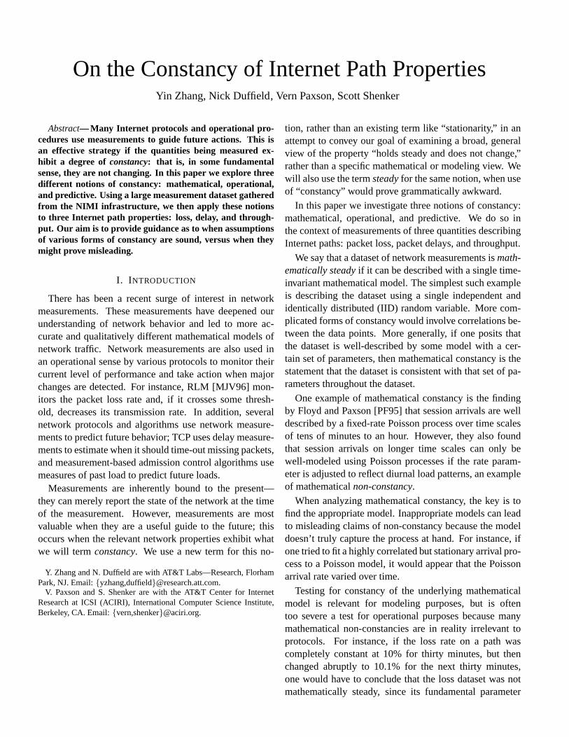
agree closely. Over all the traces there are usually just ahandful of CFRs, but for lossy traces the figure is muchlarger, with the average rising from around 5 over all tracesto around 20 over the lossy traces. Clearly, once we arein a high-loss regime, we also are in a regime of chang-ing conditions. In addition, sometimes we observe a hugenumber of CFRs. Figure 4 shows an example of the latter,a trace whose loss episode process divides into more than400 CFRs.

Once we have divided traces into one or more CFRs,we can then analyze each region separate from the others,having confidence that within the region the overall lossepisode rate does not change. Upon applying the Box-Ljung test, we find that 88-92% of the regions are con-sistent with an absence of lag 1 correlation, and 77-86%are consistent with no correlation up to lag 100. Clearly,within a CFR the loss episode process is well modeled asIID better than over the entire trace (previous section). Inaddition, applying the Anderson-Darling test (§ A-C) tothe interarrivals between loss episodes in a region, we findthat 77-85% of the regions are consistent with exponentialinterarrivals.

Together, these findings solidly support modelingloss episodes as homogeneous Poisson processes withinchange-free regions. In particular, correlations in loss pro-cesses are due to the presence of consecutive losses, ratherthan nearby losses.

It remains to describe the structure of loss episodes. Wedo so in the context of the aforementioned Gilbert and ex-tended Gilbert models. For the two-state Gilbert model tohold, we should find that within a loss episode the proba-bility of observing each additional loss remains the same.In particular, the probability that we observe a 2nd lossin an episode, given that we’ve seen the initial loss of anepisode, should be the same as the probability of observinga 3rd loss given that we’ve seen the 2nd loss. Similarly, theextended Gilbert model allows fork different loss rates forthe firstk losses after the initial loss, each correspondingto a different state in the model.

0 10 20 30 40 50

0.0

0.2

0.4

0.6

0.8

1.0

Minutes of Constancy

Cum

ulat

ive

Prob

abilit

y

1 min episodes1 min pkts10 sec episodes10 sec pkts

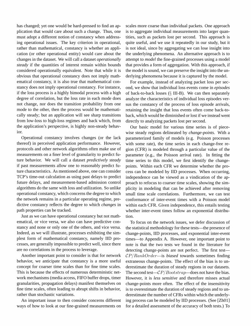
Fig. 5. Operational constancy for packet loss and loss episodes,conditioned on the constancy lasting 50 minutes or less.

Accordingly, we can assess whetherk states suffice todescribe a given loss process by seeing whether thek + 1loss after the initial loss occurs (conditioned on thekthloss) with the same probability as thekth loss does (con-ditioned on thek − 1 loss). We made these tests usingFisher’s Exact Test [Ri95], and found that, for bothW1

andW2, 40% of the traces are consistent with Bernoulliloss; 89% with the Gilbert two-state model; 98% with3 states (extended Gilbert); and 99% with 4 states. How-ever, the models work less well for lossy traces: only 6%are well-modeled as Bernoulli, 68% with 2 states, 85%with 3 states, and 96% with 4 states.

C. Operational constancy of loss rate

We now turn to analyzing a different notion of loss rateconstancy, namely from anoperationalviewpoint. To doso, we partition loss rates into the following categories:0–0.5%, 0.5–2%, 2–5%, 5–10%, 10–20%, and 20+%. Therole of these categories is to capture qualitative notionssuch as “no loss,” “minor loss,” “tolerable loss,” “seriousloss,” “very serious loss,” and “unacceptable loss.”

For each trace we then analyze how long the loss rate re-mained in the same category. Figure 5 plots the weightedCDF for four different loss series associated with eachtrace inW1: the loss episode rate computed over 1-minuteintervals, the raw packet loss rate over 1-minute intervals,and the same but computed over 10-second intervals. (Re-sults forW2 are virtually identical.) The CDF is weightedby the size of the constancy interval, as mentioned above;thus, we interpret the plot as showing the unconditionalprobability that at any given moment we would find our-selves in a constancy interval of durationT or less. Forexample, about 50% of the time we will find ourselves in aconstancy interval of 10 min or less, if what we care aboutis the constancy of loss episodes computed over minute-long intervals (solid line).

An important point is that we truncated the plot to onlyshow the distribution of intervals 50 minutes or less. Wecharacterize longer intervals separately, as these reflect

entire datasets that were operationally steady. Since ourdatasets spanned at most one hour, constancy over thewhole dataset provides a lower bound on the duration ofconstancy, rather than an exact value, and hence differsfrom the distributions in Figure 5.

For the four loss series, the corresponding probabili-ties of observing a constancy interval of 50 or more min-utes are 71%, 57%, 25%, and 22%. Thus, if we onlycare about constancy of loss viewed over 1-minute peri-ods, then about two-thirds (57–71%) of the time, we willfind we are in a constancy period of at least an hour induration—it could be quite a bit longer, as our measure-ments limited us to observing at most an hour of constancy.

We also see that the key difference between the 10 secand 1 min results is the likelihood of being in a period oflong constancy: it takes only a single 10-second changein loss rate to interrupt the hour-long interval, much morelikely than a single 1-minute change. If we condition onbeing in a shorter period of constancy, then we find verysimilar curves. In particular, if we are not in a period oflong-lived constancy, then, per the plot, we find that abouthalf the time we are in a 10-minute interval or shorter, andthere is not a great deal of difference in the duration ofconstancy, regardless of whether we consider one-minuteor 10-second constancy, or loss runs or loss episodes.

Finally, we repeated this assessment using a set of cut-points for the loss categories that fell in the middle of theabove cutpoints (e.g., 3.5–7.5%), to test for possible bin-ning effects in which some traces straddle a particular lossboundary. The results are highly similar.

D. Comparing mathematical and operational constancy

We now briefly assess the degree to which we findthat the notion of mathematical constancy of loss coin-cides with the notion of operational constancy of loss.While there are many dimensions in which we could un-dertake such an assessment, we aim here to only explorethe coarse-grained relationship.

We begin by categorizing each trace as either “steady”or “not steady,” where the distinction between the two con-cerns whether the trace has a 20-minute region of con-stancy; i.e., for mathematical constancy, a 20-minute CFRfor the rate of the loss episode process, and for operationalconstancy, a 20-minute period during which the loss ratedid not stray outside one of the particular regions. We thenassess what proportion of the traces were neither mathe-matically nor operationally steady (MO), mathematicallybut not operationally (MO), vice versa (MO), and both(MO).

For operational constancy evaluated using loss com-puted over 1 min, we findMO = 6–9%,MO = 6–15%,

MO = 2–5%, andMO = 74–83%. (The minor varia-tion in the figures depends on whether for operational con-stancy we look at loss rate or loss episode rate, and whetherwe use the first or the second set of loss categories as dis-cussed at the end of§ III-C.) Clearly, the notions of math-ematical and operational constancy mostly coincide.

However, if we instead evaluate operational constancyusing loss rates computed over 10 sec intervals, the figuresare significantly different:MO = 11%,MO = 37–45%,MO = 0.1%, andMO = 44–52%. We can summarizethe difference as:Operational constancy of packet loss co-incides with mathematical constancy on large time scalessuch as viewing how loss changes from one minute to thenext; but not nearly so well on medium time scales such aslooking at 10-second intervals.

E. Predictive constancy of loss rate

The last notion of packet loss constancy we explore isthat of predictiveconstancy, i.e., to what degree can anestimator predict future loss events?

There are a number of different loss-related events wecould be interested in predicting. Here, we confine our-selves to predicting the length of the next loss-free run. Wechose this event for two reasons: first, we do not have tobin the time series (which predicting loss rate over the nextT seconds would require); and second, there are known ap-plications for such prediction, such as TFRC [FHPW00].

The next question is what type of estimator to use. Weassess three different types popular in the literature: mov-ing average (MA), exponentially-weighted moving aver-age (EWMA) such as used by TCP [Ja88], and theS-shaped moving average estimator (SMA) used by TFRC.This last is a class of weighted moving average estimatorsthat give higher weights to more recent samples; we use asubclass that gives equal weight to the most recent half ofthe window, and linearly decayed weights for the earlierhalf; see [FHPW00] for discussion.

For each of these estimators there is a parameter thatgoverns the amount of memory of past events used by theestimator. For MA and SMA, we used window sizes of2, 4, 8, 16, 32; and for EWMA,α = 0.5, 0.25, 0.125, and0.01, whereα = 0.5 corresponds to weighting each newsample equally to the cumulative memory of previous sam-ples, andα = 0.01 weights the previous samples 99 timesas much as each new sample.

Once we’ve defined what estimator to use, we next haveto decide how to assess how well it performed. To do so,we compute:

prediction error= E

[ ∣

∣

∣

∣

log

(

predicted valueactual value

)∣

∣

∣

∣

]

Mean Prediction Error

0 2 4 6 8 10

0.0

0.2

0.4

0.6

0.8

1.0

Mean Prediction Error

0 2 4 6 8 10

0.0

0.2

0.4

0.6

0.8

1.0

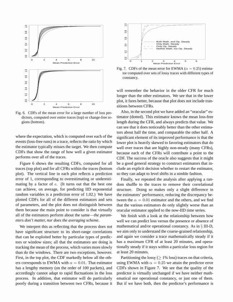
Fig. 6. CDFs of the mean error for a large number of loss pre-dictors, computed over entire traces (top) or change-free re-gions (bottom).

where the expectation, which is computed over each of theevents (loss-free runs) in a trace, reflects the ratio by whichthe estimator typically misses the target. We then computeCDFs that show the range of how well a given estimatorperforms over all of the traces.

Figure 6 shows the resulting CDFs, computed for alltraces (top plot) and for all CFRs within the traces (bottomplot). The vertical line in each plot reflects a predictionerror of 1, corresponding to overestimating or underesti-mating by a factor ofe. (It turns out that the best onecan achieve, on average, for predicting IID exponentialrandom variables is a prediction error of 1.02.) We haveplotted CDFs for all of the different estimators and setsof parameters, and the plot does not distinguish betweenthem because the main point to consider is that virtuallyall of the estimators perform about the same—the param-eters don’t matter, nor does the averaging scheme.

We interpret this as reflecting that the process does nothave significant structure to its short-range correlationsthat can be exploited better by particular types of predic-tors or window sizes; all that the estimators are doing istracking the mean of the process, which varies more slowlythan do the windows. There are two exceptions, however.First, in the top plot, the CDF markedly below all the oth-ers corresponds to EWMA withα = 0.01. That estimatorhas a lengthy memory (on the order of 100 packets), andaccordingly cannot adapt to rapid fluctuations in the lossprocess. In addition, that estimator will do particularlypoorly during a transition between two CFRs, because it

Mean Prediction Error0 1 2 3 4 5 6

0.0

0.2

0.4

0.6

0.8

1.0

Both Math. and Op. SteadyOnly Math. SteadyOnly Op. SteadyNeither Math. nor Op. Steady

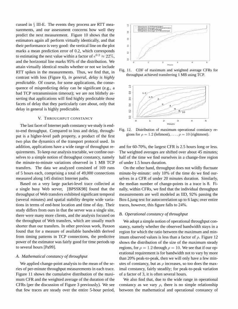
Fig. 7. CDFs of the mean error for EWMA (α = 0.25) estima-tor computed over sets of lossy traces with different types ofconstancy.

will remember the behavior in the older CFR for muchlonger than the other estimators. We see that in the lowerplot, it fares better, because that plot does not include tran-sitions between CFRs.

Also, in the second plot we have added an “oracular” es-timator (dotted). This estimator knows the mean loss-freelength during the CFR, and always predicts that value. Wecan see that it does noticeably better than the other estima-tors about half the time, and comparable the other half. Asignificant element of its improved performance is that thelower plot is heavily skewed to favoring estimators that dowell over traces that are highly non-steady (many CFRs),because each of the CFRs will contribute a point to theCDF. The success of the oracle also suggests that it mightbe a good general strategy to construct estimators that in-clude an explicit decision whether to restart the estimator,so they can adapt to level shifts in a nimble fashion.

Finally, we repeated the analysis after applying a ran-dom shuffle to the traces to remove their correlationalstructure. Doing so makes only a slight difference inthe estimators’ performance, reducing the discrepancy be-tween theα = 0.01 estimator and the others, and we findthat the various estimators do only slightly worse than anoracular estimator applied to the now-IID time series.

We finish with a look at the relationship between howwell we can predict loss versus the presence or absence ofmathematical and/or operational constancy. As in§ III-D,we aim only to understand the coarse-grained relationship,and again we consider a trace mathematically steady if ithas a maximum CFR of at least 20 minutes, and opera-tionally steady if it stays within a particular loss region forat least 20 minutes.

Partitioning the lossy (≥ 1% loss) traces on that criteria,using EWMA withα = 0.25 we attain the predictor errorCDFs shown in Figure 7. We see that the quality of thepredictor is virtually unchanged if we have neither math-ematical nor operational constancy, or just one of them.But if we have both, then the predictor’s performance is

Ratio of RTT to Median

0 50 100 150 200

10^-6

10^-4

10^-2

10^0

10:1 Ratio

1 RTT in every 1,000

Fig. 8. Complementary distribution of the ratio of RTT samplesto the median of their traces, computed forW2.

worse. This is because in this regime the loss episode pro-cess resembles an IID process without significant short-term variations, and the recent samples seen by the esti-mator provide no help in predicting the next event. In ad-dition, note that if we look at all traces rather than just thelossy traces, the estimators again do worse, because for thetype of event we are predicting (interval until the next lossepisode), traces with low loss levels provide very few sam-ples to the estimator. However, low loss is also a conditionunder which we generally won’t care about the precise-ness of the estimator, since loss events will be quite rare.In summary,predictors do equally well whether or not wehave other forms of constancy, unless we have constancyresembling an IID process with little short-term variation.

IV. D ELAY CONSTANCY

We next turn to exploring the types of constancy asso-ciated with packet delays. Mukherjee found that packetdelay along several Internet paths was well-modeled us-ing a shifted gamma distribution, but the parameters of thedistribution varied from path to path and on time scales ofhours [Mu94]. Similarly, Claffy and colleagues found thatone-way delays measured along four Internet paths exhib-ited clear level shifts and non-constancies over the courseof a day [CPB93].

For our analysis, we again use thezing Poisson packetstreams measured on the NIMI hosts. Because the NIMIhosts lack synchronized clocks, we confine our analysis tothose datasets with bidirectional packet streams. These aregenerated byzing on hostA sending “request” packetshostB, and thezing on hostB immediately respondingto each of these by sending back matching “reply” packets,facilitating round-trip measurement at hostA. The delayin zing’s response is short, usually taking 100–200µsec,occasionally rising to a few ms.

A. Delay “spikes”

The data totaled 130M RTT measurements made be-tween 613 distinct pairs of hosts. In analyzing it, the first

phenomenon we had to deal with is the presence of de-lay spikes. These are intervals (often quite short) of highlyelevated RTTs. They are rare, but if unaddressed can seri-ously skew our analysis due to their magnitude. Figure 8conveys the size and prevalence of spikes. For each trace,we computed the median of all of the RTT measurements,and then normalized each RTT measurement by dividing itby the median. This allows us to then plot all of the mea-surements together to assess, in high level terms, the mag-nitude of RTT variation present in the data. The plot showsthe complementary distribution of the RTT-to-median ra-tio; this style of plot emphasizes the upper tail. For refer-ence we have drawn lines reflecting a ratio of 10:1 (verti-cal) and a probability of10−3 (horizontal). Clearly, thereare a significant number of very large RTTs, though not somany that we would consider them anything other than anextreme upper-tail phenomenon.

To proceed with separating spikes from regular RTT be-havior, we need to devise a definition for categorizing anRTT measurement as one or the other. We were unableto find a crisp modality to exploit—the only one presentin the plot is for ratios above or below 100:1, but that cut-off point omits many spikes that we found visually—so wesettled on the following imperfect procedure: for each newRTT measurementR′, we compared it to the previous non-spike measurement,R. If R′ ≥ max(k · R, 250ms), thenwe consider the new measurement a spike; otherwise, wesetR ← R′ and continue to the next measurement.2 Wethen applied this classification fork = 2 andk = 4. Doingso revealed two anomalies: a high latency path plagued byrapid RTT fluctuations ranging from 200 ms to 1 sec, anda pair of hosts that periodically jumped their clocks. Withthe anomalies removed, we find thatk = 2 categorized1.1 · 10−3 of theW1 RTTs as spikes, andk = 4 catego-rized3.4 · 10−4.

Once we had the definition in place, we could checkit in terms of “yes, these are really outliers,” as follows:for each trace we computedx andσ, the mean and stan-dard deviation of the RTT measurementswith the spikesremoved. We then for each spike assessed how manyσit was abovex. For W1, the k = 2 definition leads tospikes that are typically (median) 16.9σ above the mean,with 80% being more than 5.6σ. Fork = 4, these figuresrise to 28σ and 6.6σ.

B. Constancy of body of RTT distribution

The degree to which RTT spikes are indeed outlierspoints up a need to assess the constancy of the body of

2We found the 250 ms lower bound necessary for applying the clas-sifier to traces with quite low RTTs.

0 10 20 30 40 50 60

0.0

0.2

0.4

0.6

0.8

1.0

Minutes

RTT Median (lossy)RTT MedianIQR Median (lossy)IQR Median

0 10 20 30 40 50 60

0.0

0.2

0.4

0.6

0.8

1.0

Minutes

RTT Median (lossy)RTT MedianIQR Median (lossy)IQR Median

Fig. 9. CDF of largest CFR for median and IQR of packet RTTdelays. “Lossy” is the same analysis restricted to traces forwhich the overall loss rate exceeded 1%.

the RTT distribution separate from that of the RTT spikes.We do so by applying change-point analysis to the medianand inter-quartile range (IQR) of the distribution.3

Figure 9 shows CDFs of the size of the largest corre-sponding CFRs. We see that, overall, the median is lesssteady than the IQR (indeed, we find that IQR change-points appear to often be a subset of median change-points), and both distributions shift about 5 minutes to theleft for lossy traces. The striking difference with Figure 3,though, is the absence of entire hours with no change-points. Thus we find thatoverall, delay is less steadythan loss, and that, while there’s a wide range in the lengthof steady delay regions, in general delay appears well de-scribed as steady on time scales of 10–30 minutes. We canalso test the median and IQR (computed over 10-secondintervals) for independence within each CFR. Using theBox-Ljung test for up to 6 lags, we find very good agree-ment (90–92%) with independence.

C. Constancy of RTT spikes

Having characterized the constancy of the packet delaydistribution’s body, we now turn to the constancy of theRTT spike process. Analogous to our approach for packetloss, we group consecutive spikes into spike episodes, not-ing that in general the episodes are quite short lived: forexample, the median duration of a spike episode (usingk = 2) in W1 was 150 ms, and the mean 275 ms.

3The IQR of a distribution is the distance between the 25th and 75thpercentiles. It serves as a robust counterpart to standard deviation.ForIQR change-points, we compute the IQR over ten-second intervals andlook for a change in the median of that time series.

Mean Prediction Error

0.0 0.5 1.0 1.5

0.0

0.2

0.4

0.6

0.8

1.0

Fig. 10. CDFs of the mean error for a large number of delaypredictors.

Upon applying change-point detection to the spikeepisode process, we find spike episodes even more steadythan loss episodes: the process is steady across the entirehour 75% of the time fork = 2 spikes, and 90% of thetime fork = 4 spikes. In addition, we find the interarrivalsbetween spikes are well-modeled as IID exponential, i.e.,Poisson.

D. Operational constancy of RTT

Similar to our analysis for loss (§ III-C), we assess theoperational constancy of RTTs by partitioning the delaysinto a set of categories and then assessing the duration ofregions over which the measured RTT stays within a singlecategory.

Different applications can have quite different views asto what constitutes good, fair, poor, etc., delay. To haveconcrete categories, we used ITU Recommendation G.114[ITU96], which defines three regions: 0–150 ms (“Accept-able for most user applications”), 150–400 ms (“Accept-able provided that Administrations are aware of the trans-mission time impact on the transmission quality of user ap-plications”), 400+ ms (“Unacceptable for general networkplanning purposes”). Because these recommendations arefor one-way delays and we are analyzing RTTs, we dou-bled them to form RTT categories, and then sub-divided0–300 ms into 0–100 ms, 100–200 ms, and 200–300 ms,to allow a somewhat finer-grained assessment.

We find that more than half of the traces have maxi-mum CFRs under 10 min, and 80% are under 20 min. Wefound virtually no difference whether or not we left RTTspikes in the traces (since they are rare), or when we testeda “shifted” version of the categories similar to the shiftedversion of loss rates discussed in§ III-C. Thus, not onlyare packet delays not mathematically steady, they also arenot operationally steady.

E. Predictive constancy of delay

We finish our assessment of different types of delay con-stancy with a brief look at the efficacy of predicting futureRTT values. We again use the families of estimators dis-

cussed in§ III-E. The events they process are RTT mea-surements, and our assessment concerns how well theypredict the next measurement. Figure 10 shows that theestimators again all perform virtually identically, and thattheir performance is very good: the vertical line on the plotmarks a mean prediction error of 0.2, which correspondsto estimating the next value within a factor ofe0.2 ≈ 22%,and the horizontal line marks 95% of the distribution. Weattain virtually identical results whether or not we includeRTT spikes in the measurements. Thus, we find that, incontrast with loss (Figure 6),in general, delay is highlypredictable. Of course, for some applications, the conse-quence of mispredicting delay can be significant (e.g., abad TCP retransmission timeout); we are not blithely as-serting that applications will find highly predictable thosefacets of delay that they particularly care about, only thatdelay in general is highly predictable.

V. THROUGHPUT CONSTANCY

The last facet of Internet path constancy we study is end-to-end throughput. Compared to loss and delay, through-put is a higher-level path property, a product of the firsttwo plus the dynamics of the transport protocol used. Inaddition, applications have a wide range of throughput re-quirements. To keep our analysis tractable, we confine our-selves to a simple notion of throughput constancy, namelythe minute-to-minute variations observed in 1 MB TCPtransfers. The data we analyzed consisted of 169 runsof 5 hours each, comprising a total of 49,000 connectionsmeasured along 145 distinct Internet paths.

Based on a very large packet-level trace collected ata single busy Web server, [BPSSK98] found that thethroughput of Web transfers exhibited significant temporal(several minutes) and spatial stability despite wide varia-tions in terms of end-host location and time of day. Theirstudy differs from ours in that the server was a single site,there were many more clients, and the analysis focused onthe throughput of Web transfers, which are usually muchshorter than our transfers. In other previous work, Paxsonfound that for a measure of available bandwidth derivedfrom timing patterns in TCP connections, the predictivepower of the estimator was fairly good for time periods upto several hours [Pa99].

A. Mathematical constancy of throughput

We applied change-point analysis to the mean of the se-ries of per-minute throughput measurements in each trace.Figure 11 shows the cumulative distribution of the maxi-mum CFR and the weighted average of the duration of theCFRs (per the discussion of Figure 3 previously). We seethat few traces are steady over the entire 5-hour period,

0 1 2 3 4 5

0.0

0.2

0.4

0.6

0.8

1.0

Hours

Maximum (CP/RankOrder)Weighted average (CP/RankOrder)Maximum (CP/Bootstrap)Weighted average (CP/Bootstrap)

Fig. 11. CDF of maximum and weighted average CFRs forthroughput achieved transferring 1 MB using TCP.

Hours

0 1 2 3 4 5

0.0

0.2

0.4

0.6

0.8

1.0

1.2

1.52

34

68

10

Fig. 12. Distribution of maximum operational constancy re-gions forρ = 1.2 (leftmost),. . . , ρ = 10 (rightmost).

and for 60-70%, the largest CFR is 2.5 hours long or less.The weighted averages are shifted over about 45 minutes;half of the time we find ourselves in a change-free regionof under 1.5 hours duration.

On the other hand, throughput does not wildly fluctuateminute-by-minute: only 10% of the time do we find our-selves in a CFR of under 20 minutes duration. Similarly,the median number of change-points in a trace is 8. Fi-nally, within CFRs, we find that the individual throughputmeasurements are well modeled as IID, 92% passing theBox-Ljung test for autocorrelation up to 6 lags; over entiretraces, however, this figure falls to 24%.

B. Operational constancy of throughput

We adopt a simple notion of operational throughput con-stancy, namely whether the observed bandwidth stays in aregion for which the ratio between the maximum and min-imum observed values is less than a factor ofρ. Figure 12shows the distribution of the size of the maximum steadyregions, forρ = 1.2 throughρ = 10. We see that if our op-erational requirement is for bandwidth not to vary by morethan 20% peak-to-peak, then we will only have a few min-utes of constancy, but asρ increases, so too does the max-imal constancy, fairly steadily; for peak-to-peak variationof a factor of 3, it is often several hours.

We also find that, due to the wide range in operationalconstancy as we varyρ, there is no simple relationshipbetween the mathematical and operational constancy of

Mean Prediction Error

0.0 0.2 0.4 0.6 0.8 1.0 1.2

0.0

0.2

0.4

0.6

0.8

1.0

LongMemory

Short Memory

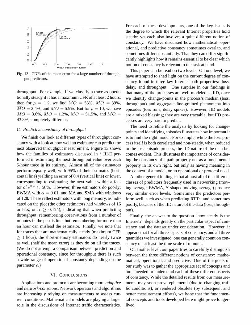
Fig. 13. CDFs of the mean error for a large number of through-put predictors.

throughput. For example, if we classify a trace as opera-tionally steady if it has a maximum CFR of at least 2 hours,then for ρ = 1.2, we find MO = 53%, MO = 39%,MO = 2.4%, andMO = 5.9%. But forρ = 10, we haveMO = 3.6%,MO = 1.2%,MO = 51.5%, andMO =43.8%, completely different.

C. Predictive constancy of throughput

We finish our look at different types of throughput con-stancy with a look at how well an estimator can predict thenext observed throughput measurement. Figure 13 showshow the families of estimators discussed in§ III-E per-formed in estimating the next throughput value over each5-hour trace in its entirety. Almost all of the estimatorsperform equally well, with 95% of their estimates (hori-zontal line) yielding an error of 0.4 (vertical line) or lower,corresponding to estimating the next value within a fac-tor of e0.4 ≈ 50%. However, three estimators do poorly:EWMA with α = 0.01, and MA and SMA with windowsof 128. These reflect estimators with long memory, as indi-cated on the plot (the other estimators had windows of 16or less, orα ≥ 0.125), indicating that when predictingthroughput, remembering observations from a number ofminutes in the past is fine, but remembering for more thanan hour can mislead the estimator. Finally, we note thatfor traces that are mathematically steady (maximum CFR≥ 1 hour), the short-memory estimators do nearly twiceas well (half the mean error) as they do on all the traces.(We do not attempt a comparison between prediction andoperational constancy, since for throughput there is sucha wide range of operational constancy depending on theparameterρ.)

VI. CONCLUSIONS

Applications and protocols are becoming moreadaptiveandnetwork-conscious. Network operators and algorithmsare increasingly relying on measurements to assess cur-rent conditions. Mathematical models are playing a largerrole in the discussions of Internet traffic characteristics.

For each of these developments, one of the key issues isthe degree to which the relevant Internet properties holdsteady; yet each also involves a quite different notion ofconstancy. We have discussed how mathematical, oper-ational, and predictive constancy sometimes overlap, andsometimes differ substantially. That they can differ signifi-cantly highlights how it remains essential to be clear whichnotion of constancy is relevant to the task at hand.

This paper can be read on two levels. On one level, wehave attempted to shed light on the current degree of con-stancy found in three key Internet path properties: loss,delay, and throughput. One surprise in our findings isthat many of the processes are well-modeled as IID, oncewe identify change-points in the process’s median (loss,throughput) and aggregate fine-grained phenomena intoepisodes (loss runs, delay spikes). However, IID modelsare a mixed blessing; they are very tractable, but IID pro-cesses are very hard to predict.

The need to refine the analysis by looking for change-points and identifying episodes illustrates how important itis to find the right model. For example, while the loss pro-cess itself is both correlated and non-steady, when reducedto the loss episode process, the IID nature of the data be-comes evident. This illustrates the importance of consider-ing the constancy of a path property not as a fundamentalproperty in its own right, but only as having meaning inthe context of a model, or an operational or protocol need.

Another general finding is that almost all of the differentclasses of predictors frequently used in networking (mov-ing average, EWMA,S-shaped moving average) producevery similar error levels. Sometimes the predictors per-form well, such as when predicting RTTs, and sometimespoorly, because of the IID nature of the data (loss, through-put).

Finally, the answer to the question “how steady is theInternet?” depends greatly on the particular aspect of con-stancy and the dataset under consideration. However, itappears that for all three aspects of constancy, and all threequantities we investigated, one can generally count on con-stancy on at least the time scale of minutes.

On another level, our paper tries to carefully distinguishbetween the three different notions of constancy: mathe-matical, operational, and predictive. One of the goals ofour study was to gather the appropriate set of concepts andtools needed to understand each of these different aspectsof constancy. While the detailed results from our measure-ments may soon prove ephemeral (due to changing traf-fic conditions), or rendered obsolete (by subsequent andbetter measurement efforts), we hope that the fundamen-tal concepts and tools developed here might prove longer-lived.

VII. A CKNOWLEDGMENTS

Many thanks to Andrew Adams, who did a tremendousamount of NIMI development work to support our ex-tensive measurements, and to his NIMI colleagues, MattMathis and Jamshid Mahdavi. We would also like to thankLee Breslau for valuable discussions; the many NIMI vol-unteers who host NIMI measurement servers; and MarkAllman for the bulk-transfer measurement software, andcomments on this work.

APPENDIX

I. STATISTICAL METHODOLOGY

In this appendix we discuss the three main statistical tech-niques we use in our analysis, tests for: change-points, indepen-dence, and exponential interarrivals.

A. Testing for change-points

We apply two different tests, CP/RankOrder andCP/Bootstrap, to detect changes in the median. Both tests de-tect change-points in a two step approach: first identifyingacandidate change-point, then applying a statistical test to deter-mine whether it is significant. The combined approach [La96],[Ta00] uses an analysis of ranks in order to detect changes inthe median [SC88]. Being based on ranks, the method is re-sistant, i.e., tolerant to the presence of outliers. Furthermore,the hypotheses underlying these test are quite weak; equality ofvariances is not required.

Consider first a set ofn values(xi)i=1,...,n comprising a seg-ment of a given time series. Construct the rankri of eachxi

within the set, i.e.,1 for the smallest andn for the largest. Com-pute the cumulative rank sumssi =

∑ij=1

ri. The basis ofthe test is that if no change point is present, the cumulativeranksumssi should increase roughly linearly withi. Indeed, supposewe form the adjusted sum:

s′i = |si − si|

as the difference betweensi, and its presumed meansi = i(n +1)/2 assuming no change-point to be present. Thens′i shouldstay close to zero. If, however, a change-point is present, higherranks should predominate in either the earlier or later partof theset, and hences′i will climb to a maximum before decreasing tozero ati = n. We identify the maximizing indexi0 for s′i andirunning over{1, . . . , n} as a candidate change-point.

In the second stage, to test equality of two setsX− ={x1, . . . , xi0−1} andX+ = {xi0+1, . . . , xn}, CP/Bootstrapuses the bootstrap analysis procedure outlined in [Ta00], whileCP/RankOrder uses the Fligner-Policello Robust Rank-OrderTest [SC88].• Bootstrap analysis(used inCP/Bootstrap). The bootstrapanalysis procedure outlined in [Ta00] usesSdiff , defined as(max si − min si), to estimate the magnitude of the change atthe candidate change-point. It determines the confidence levelof change by testing how often the bootstrap differenceS0

diffof a bootstrap sample{x0

i }—a random permutation of{xi}—isless than the original differenceSdiff .

• Fligner-Policello Robust Rank-Order Test(used inCP/Rank−Order). The test statistic is constructed as follows. Forx ∈ X+

definer+x as the rank ofx in X+ ∪ X− minus the rank ofx in

X+, with rank ties handled by assigning the average rank to allmembers of a tie set. Define rank meanr+ =

∑

x∈X+ r+x /n+

wheren+ = #X+, and sums of squared differencesv+ =∑

x∈X+(r+x − r+)2. Definen−, r−, andv− symmetrically.

Then the test statistic:

z =n+r+ − n−r−

2√

r+r− + v+ + v−

has, asymptotically asn → ∞, a standard normal distribution.Thus we can associate a significance level with the candidatechange pointi0 in the usual manner. By choosing a significancelevel ℓ (we use5% throughout this thesis) we specify our ac-ceptable probabilityℓ of incorrectly rejecting the null hypothe-sis. The test accepts the null hypothesis (in a two-sided test) ifF (|z|) < 1 − ℓ/2 whereF is the cumulative distribution func-tion of the standard normal distribution. (However, note thatthe largen asymptotic is not sufficiently accurate wheni0 andn−i0 ≤ 12; in this case Table K in Appendix I of [SC88] shouldbe used.) In some cases we shall use this test on binary data, inwhich case it reduces to a test of the equality of the expectationscorresponding to binary states on either side of the candidatechange-point.

The above can be extended to the identification of multiplechange points, as follows [La96], [Ta00]. First, choose a sig-nificance level. Second, apply the above method recursivelyto the two segments{1, . . . , i0} and{i0 + 1, . . . , n} until nomore change points are found at the chosen significance level.Third, apply backward elimination to reinspect the set of candi-date change points in order to eliminate false detections, as fol-lows. Let there bem change-point candidatesj1 < · · · < jm.Let j0 andjm+1 be 0 andn respectively. Starting with the firstidentified candidate, call itjk0

(1 ≤ k0 ≤ m), reinspect forchange-points on the set{jk0−1 + 1, . . . , jk0+1}, and adjust ordelete non-significant change-points. Repeat for all candidatesin order of identification. Repeat backward elimination untilthe number of change-points is stable. By reestimating eachchange-point using only the data between the two surroundingchange-points, backward elimination avoids the contaminationcaused by the presence of multiple change-points at the timeofrecursion and consequently helps to reduce the rate of falsede-tections.

B. Testing for independence

We assess independence using the Box-Ljung test [LB78].For a time series withn elements, the Box-Ljung statisticQk isa weighted sum of squares of measured autocorrelationsri fromlags1 up tok:

Qk = n(n + 2)

k∑

i=1

r2i

n − i.

Under the null hypothesis that the process comprises indepen-dent Gaussian random variables, the distribution ofQk con-verges, for largen, to aχ2 distribution withk degrees of free-dom. Thus by comparing the test statisticQk with the 1 − ℓ

quantile of the appropriateχ2 distribution, we can test whetherthe autocorrelations of the time series differ at significance levelℓ from those of independent Gaussian random variables. In fact,as remarked in [LB78], the test is relatively insensitive todepar-tures from the Gaussian hypothesis in the underlying process.This is because the measured autocorrelationsri are asymptoti-cally Gaussian provided the marginal distribution of the under-lying process has finite variance. (While infinite variance (heavytails) abound in networking behavior, the time series we con-sider here are generally well bounded, and certainly have finitevariance.)

C. Testing for exponential distributions

An exploratory test for an exponential distribution of inter-event times is to plot the log-complementary distribution func-tion; for an exponential distribution this is linear with slopeequal to the negative of the reciprocal of the mean. A statisticaltest is that of Anderson-Darling. This test has been found tobemore powerful than either the Kolmogorov-Smirnov or theχ2

tests, i.e., its probability of correctly rejecting the null hypoth-esis (that the distribution is exponential) is greater; see[DS86].This is, in part, due to the fact that the Anderson-Darling testemploys the full empirical distribution (rather than binning, asin a χ2 test), allowing it to give more weight to larger samplevalues whose presence can lead to a violation of the null hy-pothesis.

For a set ofn rank-ordered inter-event timest1 < · · · < tn,the appropriate Anderson-Darling statistic is:

A2 = −n − 1

n

n∑

i=1

(2i − 1){

log(1 − e−ti/t) − tn+1−i/t}

wheret = n−1∑n

i=1ti is the empirical mean inter-event time.

We reject the null hypothesis at significance levelℓ if the teststatistic exceeds the tabulated values appropriate for that level;see, e.g., Table 4.11 in [DS86]. We note the importance of usingthe table appropriate to the present case in which the mean ises-timated from the sample, rather than being specified in advance.Moreover, the table explicitly takes into account the effect of afinite sample sizen.

REFERENCES

[BPSSK98] H. Balakrishnan, V. Padmanabhan, S. Seshan, M. Stemmand R. Katz, “TCP Behavior of a Busy Web Server: Analysisand Improvements,”Proc. IEEE INFOCOM ’98, Mar. 1998.

[Bo93] J-C. Bolot, “End-to-End Packet Delay and Loss Behav-ior in the Internet,” Proc. SIGCOMM ’93, pp. 289–298,Sept. 1993.

[CPB93] K. Claffy, G. Polyzos and H-W. Braun, “Measurement Con-siderations for Assessing Unidirectional Latencies,”Inter-networking: Research and Experience, 4 (3), pp. 121–132,Sept. 1993.

[DS86] R.B. D’Agostino and M.A. Stephens, Eds.,Goodness-of-FitTechniques, Marcel Dekker, New York, 1986.

[FHPW00] S. Floyd, M. Handley, J. Padhye and J. Widmer,“Equation-Based Congestion Control for Unicast Applica-tions,” Proc. SIGCOMM ’00, pp. 43–56, Aug. 2000.

[Gi60] E. Gilbert, “Capacity of a Burst-Noise Channel,”Bell Sys-tems Technical Journal, 39(5), pp. 1253–1265, Septem-ber 1960.

[ITU96] International Telecommunication Union, “One-way Trans-mission Time,”ITU Recommendation G.114, Feb. 1996.

[Ja88] V. Jacobson, “Congestion Avoidance and Control,”Proc.SIGCOMM ’88, pp. 314-329, Aug. 1988.

[JBB92] V. Jacobson, R. Braden, and D. Borman, “TCP Extensionsfor High Performance,” RFC-1323, May 1992.

[JS00] W. Jiang and H. Schulzrinne, “Modeling of Packet Loss andDelay and Their Effect on Real-Time Multimedia ServiceQuality,” Proc. NOSSDAV 2000, June 2000.

[La96] J. Lanzante, “Resistant, robust and non-parametric tech-niques for the analysis of climate data: theory and examples,including applications to historical radiosonde station data,”Int. J. Climatol., 16 (11), 1197-1226, 1996.

[LB78] G. Ljung, and G. Box “On a Measure of Lack of Fit in TimeSeries Models,”Biometrika ’65, pp. 297–303, 1978.

[MJV96] S. McCanne, V. Jacobson, and M. Vetterli, “Receiver-drivenLayered Multicast,” Proc. SIGCOMM ’96, pp. 117–130,Aug. 1996.

[Mu94] A. Mukherjee, “On the Dynamics and Significance of LowFrequency Components of Internet Load,”Internetworking:Research and Experience, Vol. 5, pp. 163–205, Decem-ber 1994.

[PF95] V. Paxson, and S. Floyd, “Wide-Area Traffic: The Failureof Poisson Modeling,”IEEE/ACM Transactions on Network-ing, 3(3), pp. 226-244, June 1995.

[PMAM98] V. Paxson, J. Mahdavi, A. Adams, and M. Mathis, “AnArchitecture for Large-Scale Internet Measurement,”IEEECommunications, 36(8), pp 48–54, Aug. 1998.

[Pa99] V. Paxson, “End-to-End Internet Packet Dynamics,”IEEE/ACM Transactions on Networking, 7(3), pp. 277–292,June 1999.

[Ri95] J. Rice, “Mathematical Statistics and Data Analysis,” 2ndedition, Duxbury Press, 1995.

[SCK00] H. Sanneck, G. Carle, and R. Koodli, “A framework modelfor packet loss metrics based on loss run length,”Proc.SPIE/ACM SIGMM Multimedia Computing and NetworkingConference, January 2000.

[SC88] S. Siegel and N. Castellan,Non-parametric statistics for thebehavioral sciences, McGraw–Hill, New York, 1988.

[Ta00] W.A. Taylor, “Change-Point Analysis: A Powerful NewTool For Detecting Changes”, preprint, available as http://www.variation.com/cpa/tech/changepoint.html

[Wo82] R. Wolff, “Poisson Arrivals See Time Averages,”OperationsResearch, 30(2), pp. 223–231, 1982.

[YMKT99] M. Yajnik, S. Moon, J. Kurose and D. Towsley, “Measure-ment and Modeling of the Temporal Dependence in PacketLoss,”Proc. IEEE INFOCOM ’99, Mar. 1999.

[ZPS00] Y. Zhang, V. Paxson and S. Shenker, “The Stationarity ofInternet Path Properties: Routing, Loss, and Throughput,”ACIRI Technical Report, May 2000. http://www.aciri.org/vern/papers/stationarity-May00.ps.gz

[Zh01] Y. Zhang, “Characterizing End-to-End Internet Perfor-mance,” Ph.D. Thesis, Cornell University, Aug. 2001. http://www.cs.cornell.edu/yzhang/papers/thesis.ps.gz