Yet another Haskell tutorial
192
Yet Another Haskell Tutorial Hal Daum´ e III Copyright (c) Hal Daume III, 2002-2006. The preprint version of this tutorial is intended to be free to the entire Haskell community, so we grant permission to copy and distribute it for any purpose, provided that it is reproduced in its entirety, in- cluding this notice. Modified versions may not be distributed without prior concent of the author, and must still maintain a copy of this notice. The author retains the right to change or modify this copyright at any time, as well as to make the book no longer free of charge.
description
This is aimed at the beginner programmer to Haskell.
Transcript of Yet another Haskell tutorial

Yet Another Haskell Tutorial
Hal Daume III
Copyright (c) Hal Daume III, 2002-2006. The preprint version of this tutorial isintended to be free to the entire Haskell community, so we grant permission to copyand distribute it for any purpose, provided that it is reproduced in its entirety, in-cluding this notice. Modified versions may not be distributed without prior concentof the author, and must still maintain a copy of this notice. The author retains theright to change or modify this copyright at any time, as well as to make the book nolonger free of charge.
About This Report
The goal of the Yet Another Haskell Tutorial is to provide a complete intoduction tothe Haskell programming language. It assumes no knowledge of the Haskell languageor familiarity with functional programming in general. However, general familiaritywith programming concepts (such as algorithms) will be helpful. This is not intendedto be an introduction to programming in general; rather, to programming in Haskell.Sufficient familiarity with your operating system and a text editor is also necessary(this report only discusses installation on configuration on Windows and *Nix system;other operating systems may be supported – consult the documentation of your chosencompiler for more information on installing on other platforms).
What is Haskell?
Haskell is called a lazy, pure functional programming language. It is called lazy be-cause expressions which are not needed to determine the answer to a problem are notevaluated. The opposize of lazy is strict, which is the evaluation strategry of mostcommon programming languages (C, C++, Java, even ML). A strict language is one inwhich every expression is evaluated, whether the result of its computation is importantor not. (This is probably not entirely true as optimizing compilers for strict languagesoften do what’s called “dead code elmination” – this removes unused expressions fromthe program.) It is called pure because it does not allow side effects (A side effectis something that affects the “state” of the world. For instance, a function that printssomething to the screen is said to be side-effecting, as is a function which affects thevalue of a global variable.) – of course, a programming language without side effectswould be horribly useless; Haskell uses a system of monads to isolate all impure com-putations from the rest of the program and perform them in the safe way (see Chapter 9for a discussion of monads proper or Chapter 5 for how to do input/output in a purelanguage).
Haskell is called a functional language because the evaluation of a program isequivalent to evaluating a function in the pure mathematical sense. This also differsfrom standard languages (like C and Java) which evaluate a sequence of statements,one after the other (this is termed an imperative langauge).
i

ii
The History of Haskell
The history of Haskell is best described using the words of the authors. The followingtext is quoted from the published version of the Haskell 98 Report:
In September of 1987 a meeting was held at the conference on FunctionalProgramming Languages and Computer Architecture (FPCA ’87) in Port-land, Oregon, to discuss an unfortunate situation in the functional pro-gramming community: there had come into being more than a dozen non-strict, purely functional programming languages, all similar in expressivepower and semantic underpinnings. There was a strong consensus at thismeeting that more widespread use of this class of functional languages wasbeing hampered by the lack of a common language. It was decided that acommittee should be formed to design such a language, providing fastercommunication of new ideas, a stable foundation for real applications de-velopment, and a vehicle through which others would be encouraged touse functional languages. This document describes the result of that com-mittee’s efforts: a purely functional programming language called Haskell,named after the logician Haskell B. Curry whose work provides the logicalbasis for much of ours.
The committee’s primary goal was to design a language that satisfied theseconstraints:
1. It should be suitable for teaching, research, and applications, includ-ing building large systems.
2. It should be completely described via the publication of a formalsyntax and semantics.
3. It should be freely available. Anyone should be permitted to imple-ment the language and distribute it to whomever they please.
4. It should be based on ideas that enjoy a wide consensus.
5. It should reduce unnecessary diversity in functional programminglanguages.
The committee intended that Haskell would serve as a basis for futureresearch in language design, and hoped that extensions or variants of thelanguage would appear, incorporating experimental features.
Haskell has indeed evolved continuously since its original publication. Bythe middle of 1997, there had been four iterations of the language design(the latest at that point being Haskell 1.4). At the 1997 Haskell Workshopin Amsterdam, it was decided that a stable variant of Haskell was needed;this stable language is the subject of this Report, and is called “Haskell98”.
Haskell 98 was conceived as a relatively minor tidy-up of Haskell 1.4,making some simplifications, and removing some pitfalls for the unwary.

iii
It is intended to be a “stable” language in sense the implementors are com-mitted to supporting Haskell 98 exactly as specified, for the foreseeablefuture.
The original Haskell Report covered only the language, together with astandard library called the Prelude. By the time Haskell 98 was stabilised,it had become clear that many programs need access to a larger set of li-brary functions (notably concerning input/output and simple interactionwith the operating system). If these program were to be portable, a set oflibraries would have to be standardised too. A separate effort was there-fore begun by a distinct (but overlapping) committee to fix the Haskell 98Libraries.
Why Use Haskell?
Clearly you’re interested in Haskell since you’re reading this tutorial. There are manymotivations for using Haskell. My personal reason for using Haskell is that I havefound that I write more bug-free code in less time using Haskell than any other lan-guage. I also find it very readable and extensible.
Perhaps most importantly, however, I have consistently found the Haskell commu-nity to be incredibly helpful. The language is constantly evolving (that’s not to sayit’s instable; rather that there are numerous extensions that have been added to somecompilers which I find very useful) and user suggestions are often heeded when newextensions are to be implemented.
Why Not Use Haskell?
My two biggest complaints, and the complaints of most Haskellers I know, are: (1) thegenerated code tends to be slower than equivalent programs written in a language likeC; and (2) it tends to be difficult to debug.
The second problem tends not be to a very big issue: most of the code I’ve writtenis not buggy, as most of the common sources of bugs in other languages simply don’texist in Haskell. The first issue certainly has come up a few times in my experience;however, CPU time is almost always cheaper than programmer time and if I have towait a little longer for my results after having saved a few days programming anddebugging.
Of course, this isn’t the case of all applications. Some people may find that thespeed hit taken for using Haskell is unbearable. However, Haskell has a standardizedforeign-function interface which allow you to link in code written in other languages,for when you need to get the most speed out of your code. If you don’t find thissufficient, I would suggest taking a look at the language O’Caml, which often out-performs even C++, yet also has many of the benefits of Haskell.

iv
Target Audience
There have been many books and tutorials written about Haskell; for a (nearly) com-plete list, visit the http://haskell.org/bookshelf (Haskell Bookshelf) at theHaskell homepage. A brief survey of the tutorials available yields:
• A Gentle Introduction to Haskell is an introduction to Haskell, given that thereader is familiar with functional programming en large.
• Haskell Companion is a short reference of common concepts and definitions.
• Online Haskell Course is a short course (in German) for beginning with Haskell.
• Two Dozen Short Lessons in Haskell is the draft of an excellent textbook thatemphasizes user involvement.
• Haskell Tutorial is based on a course given at the 3rd International SummerSchool on Advanced Functional Programming.
• Haskell for Miranda Programmers assumes knowledge of the language Miranda.
• PLEAC-Haskell is a tutorial in the style of the Perl Cookbook.
Though all of these tutorials is excellent, they are on their own incomplete: The“Gentle Introduction” is far too advanced for beginning Haskellers and the others tendto end too early, or not cover everything. Haskell is full of pitfalls for new programmersand experienced non-functional programmers alike, as can be witnessed by readingthrough the archives of the Haskell mailing list.
It became clear that there is a strong need for a tutorial which is introductory in thesense that it does not assume knowledge of functional programming, but which is ad-vanced in the sense that it does assume some background in programming. Moreover,none of the known tutorials introduce input/output and iteractivity soon enough (PaulHudak’s book is an exception in that it does introduce IO by page 35, though the focusand aim of that book and this tutorial are very different). This tutorial is not for begin-ning programmers; some experience and knowledge of programming and computers isassumed (though the appendix does contain some background information).
The Haskell language underwent a standardization process and the result is calledHaskell 98. The majority of this book will cover the Haskell 98 standard. Any de-viations from the standard will be noted (for instance, many compilers offer certainextensions to the standard which are useful; some of these may be discussed).
The goals of this tutorial are:
• to be practical above all else
• to provide a comprehensive, free introduction to the Haskell language
• to point out common pitfalls and their solutions
• to provide a good sense of how Haskell can be used in the real world

v
Additional Online Sources of Information
A Short Introduction to Haskell :http://haskell.org/aboutHaskell.html
Haskell Wiki :http://haskell.org/hawiki/
Haskell-Tutorial :ftp://ftp.geoinfo.tuwien.ac.at/navratil/HaskellTutorial.pdf
Tour of the Haskell Prelude :http://www.cs.uu.nl/˜afie/haskell/tourofprelude.html
Courses in Haskell :http://haskell.org/classes/
Acknowledgements
It would be inappropriate not to give credit also to the original designers of Haskell.Those are: Arvind, Lennart Augustsson, Dave Barton, Brian Boutel, Warren Burton,Jon Fairbairn, Joseph Fasel, Andy Gordon, Maria Guzman, Kevin Hammond, RalfHinze, Paul Hudak, John Hughes, Thomas Johnsson, Mark Jones, Dick Kieburtz, JohnLaunchbury, Erik Meijer, Rishiyur Nikhil, John Peterson, Simon Peyton Jones, MikeReeve, Alastair Reid, Colin Runciman, Philip Wadler, David Wise, Jonathan Young.
Finally, I would like to specifically thank Simon Peyton Jones, Simon Marlow,John Hughes, Alastair Reid, Koen Classen, Manuel Chakravarty, Sigbjorn Finne andSven Panne, all of whom have made my life learning Haskell all the more enjoyable byalways being supportive. There were doubtless others who helped and are not listed,but these are those who come to mind.
Also thanks to the many people who have reported “bugs” in the first edition.- Hal Daume III

vi

Contents
1 Introduction 3
2 Getting Started 52.1 Hugs . . . . . . . . . . . . . . . . . . . . . . . . . . . . . . . . . . . 5
2.1.1 Where to get it . . . . . . . . . . . . . . . . . . . . . . . . . 62.1.2 Installation procedures . . . . . . . . . . . . . . . . . . . . . 62.1.3 How to run it . . . . . . . . . . . . . . . . . . . . . . . . . . 62.1.4 Program options . . . . . . . . . . . . . . . . . . . . . . . . 72.1.5 How to get help . . . . . . . . . . . . . . . . . . . . . . . . . 7
2.2 Glasgow Haskell Compiler . . . . . . . . . . . . . . . . . . . . . . . 72.2.1 Where to get it . . . . . . . . . . . . . . . . . . . . . . . . . 72.2.2 Installation procedures . . . . . . . . . . . . . . . . . . . . . 82.2.3 How to run the compiler . . . . . . . . . . . . . . . . . . . . 82.2.4 How to run the interpreter . . . . . . . . . . . . . . . . . . . 82.2.5 Program options . . . . . . . . . . . . . . . . . . . . . . . . 92.2.6 How to get help . . . . . . . . . . . . . . . . . . . . . . . . . 9
2.3 NHC . . . . . . . . . . . . . . . . . . . . . . . . . . . . . . . . . . . 92.3.1 Where to get it . . . . . . . . . . . . . . . . . . . . . . . . . 92.3.2 Installation procedures . . . . . . . . . . . . . . . . . . . . . 92.3.3 How to run it . . . . . . . . . . . . . . . . . . . . . . . . . . 92.3.4 Program options . . . . . . . . . . . . . . . . . . . . . . . . 92.3.5 How to get help . . . . . . . . . . . . . . . . . . . . . . . . . 9
2.4 Editors . . . . . . . . . . . . . . . . . . . . . . . . . . . . . . . . . . 9
3 Language Basics 113.1 Arithmetic . . . . . . . . . . . . . . . . . . . . . . . . . . . . . . . . 133.2 Pairs, Triples and More . . . . . . . . . . . . . . . . . . . . . . . . . 143.3 Lists . . . . . . . . . . . . . . . . . . . . . . . . . . . . . . . . . . . 15
3.3.1 Strings . . . . . . . . . . . . . . . . . . . . . . . . . . . . . 173.3.2 Simple List Functions . . . . . . . . . . . . . . . . . . . . . 18
3.4 Source Code Files . . . . . . . . . . . . . . . . . . . . . . . . . . . . 203.5 Functions . . . . . . . . . . . . . . . . . . . . . . . . . . . . . . . . 22
3.5.1 Let Bindings . . . . . . . . . . . . . . . . . . . . . . . . . . 273.5.2 Infix . . . . . . . . . . . . . . . . . . . . . . . . . . . . . . . 28
vii

viii CONTENTS
3.6 Comments . . . . . . . . . . . . . . . . . . . . . . . . . . . . . . . . 283.7 Recursion . . . . . . . . . . . . . . . . . . . . . . . . . . . . . . . . 293.8 Interactivity . . . . . . . . . . . . . . . . . . . . . . . . . . . . . . . 31
4 Type Basics 374.1 Simple Types . . . . . . . . . . . . . . . . . . . . . . . . . . . . . . 374.2 Polymorphic Types . . . . . . . . . . . . . . . . . . . . . . . . . . . 394.3 Type Classes . . . . . . . . . . . . . . . . . . . . . . . . . . . . . . 40
4.3.1 Motivation . . . . . . . . . . . . . . . . . . . . . . . . . . . 404.3.2 Equality Testing . . . . . . . . . . . . . . . . . . . . . . . . 414.3.3 The Num Class . . . . . . . . . . . . . . . . . . . . . . . . . 414.3.4 The Show Class . . . . . . . . . . . . . . . . . . . . . . . . . 41
4.4 Function Types . . . . . . . . . . . . . . . . . . . . . . . . . . . . . 424.4.1 Lambda Calculus . . . . . . . . . . . . . . . . . . . . . . . . 424.4.2 Higher-Order Types . . . . . . . . . . . . . . . . . . . . . . 424.4.3 That Pesky IO Type . . . . . . . . . . . . . . . . . . . . . . . 444.4.4 Explicit Type Declarations . . . . . . . . . . . . . . . . . . . 454.4.5 Functional Arguments . . . . . . . . . . . . . . . . . . . . . 46
4.5 Data Types . . . . . . . . . . . . . . . . . . . . . . . . . . . . . . . 474.5.1 Pairs . . . . . . . . . . . . . . . . . . . . . . . . . . . . . . . 474.5.2 Multiple Constructors . . . . . . . . . . . . . . . . . . . . . 494.5.3 Recursive Datatypes . . . . . . . . . . . . . . . . . . . . . . 514.5.4 Binary Trees . . . . . . . . . . . . . . . . . . . . . . . . . . 514.5.5 Enumerated Sets . . . . . . . . . . . . . . . . . . . . . . . . 524.5.6 The Unit type . . . . . . . . . . . . . . . . . . . . . . . . . . 53
4.6 Continuation Passing Style . . . . . . . . . . . . . . . . . . . . . . . 53
5 Basic Input/Output 575.1 The RealWorld Solution . . . . . . . . . . . . . . . . . . . . . . . . 575.2 Actions . . . . . . . . . . . . . . . . . . . . . . . . . . . . . . . . . 585.3 The IO Library . . . . . . . . . . . . . . . . . . . . . . . . . . . . . 625.4 A File Reading Program . . . . . . . . . . . . . . . . . . . . . . . . 64
6 Modules 676.1 Exports . . . . . . . . . . . . . . . . . . . . . . . . . . . . . . . . . 676.2 Imports . . . . . . . . . . . . . . . . . . . . . . . . . . . . . . . . . 696.3 Hierarchical Imports . . . . . . . . . . . . . . . . . . . . . . . . . . 706.4 Literate Versus Non-Literate . . . . . . . . . . . . . . . . . . . . . . 71
6.4.1 Bird-scripts . . . . . . . . . . . . . . . . . . . . . . . . . . . 716.4.2 LaTeX-scripts . . . . . . . . . . . . . . . . . . . . . . . . . . 72
7 Advanced Features 737.1 Sections and Infix Operators . . . . . . . . . . . . . . . . . . . . . . 737.2 Local Declarations . . . . . . . . . . . . . . . . . . . . . . . . . . . 747.3 Partial Application . . . . . . . . . . . . . . . . . . . . . . . . . . . 767.4 Pattern Matching . . . . . . . . . . . . . . . . . . . . . . . . . . . . 80

CONTENTS ix
7.5 Guards . . . . . . . . . . . . . . . . . . . . . . . . . . . . . . . . . . 837.6 Instance Declarations . . . . . . . . . . . . . . . . . . . . . . . . . . 85
7.6.1 The Eq Class . . . . . . . . . . . . . . . . . . . . . . . . . . 857.6.2 The Show Class . . . . . . . . . . . . . . . . . . . . . . . . 867.6.3 Other Important Classes . . . . . . . . . . . . . . . . . . . . 877.6.4 Class Contexts . . . . . . . . . . . . . . . . . . . . . . . . . 897.6.5 Deriving Classes . . . . . . . . . . . . . . . . . . . . . . . . 89
7.7 Datatypes Revisited . . . . . . . . . . . . . . . . . . . . . . . . . . . 907.7.1 Named Fields . . . . . . . . . . . . . . . . . . . . . . . . . . 90
7.8 More Lists . . . . . . . . . . . . . . . . . . . . . . . . . . . . . . . . 927.8.1 Standard List Functions . . . . . . . . . . . . . . . . . . . . 927.8.2 List Comprehensions . . . . . . . . . . . . . . . . . . . . . . 94
7.9 Arrays . . . . . . . . . . . . . . . . . . . . . . . . . . . . . . . . . . 967.10 Finite Maps . . . . . . . . . . . . . . . . . . . . . . . . . . . . . . . 977.11 Layout . . . . . . . . . . . . . . . . . . . . . . . . . . . . . . . . . . 997.12 The Final Word on Lists . . . . . . . . . . . . . . . . . . . . . . . . 99
8 Advanced Types 1038.1 Type Synonyms . . . . . . . . . . . . . . . . . . . . . . . . . . . . . 1038.2 Newtypes . . . . . . . . . . . . . . . . . . . . . . . . . . . . . . . . 1048.3 Datatypes . . . . . . . . . . . . . . . . . . . . . . . . . . . . . . . . 105
8.3.1 Strict Fields . . . . . . . . . . . . . . . . . . . . . . . . . . . 1058.4 Classes . . . . . . . . . . . . . . . . . . . . . . . . . . . . . . . . . 108
8.4.1 Pong . . . . . . . . . . . . . . . . . . . . . . . . . . . . . . 1088.4.2 Computations . . . . . . . . . . . . . . . . . . . . . . . . . . 109
8.5 Instances . . . . . . . . . . . . . . . . . . . . . . . . . . . . . . . . 1138.6 Kinds . . . . . . . . . . . . . . . . . . . . . . . . . . . . . . . . . . 1158.7 Class Hierarchies . . . . . . . . . . . . . . . . . . . . . . . . . . . . 1178.8 Default . . . . . . . . . . . . . . . . . . . . . . . . . . . . . . . . . 117
9 Monads 1199.1 Do Notation . . . . . . . . . . . . . . . . . . . . . . . . . . . . . . . 1209.2 Definition . . . . . . . . . . . . . . . . . . . . . . . . . . . . . . . . 1229.3 A Simple State Monad . . . . . . . . . . . . . . . . . . . . . . . . . 1249.4 Common Monads . . . . . . . . . . . . . . . . . . . . . . . . . . . . 1309.5 Monadic Combinators . . . . . . . . . . . . . . . . . . . . . . . . . 1349.6 MonadPlus . . . . . . . . . . . . . . . . . . . . . . . . . . . . . . . 1379.7 Monad Transformers . . . . . . . . . . . . . . . . . . . . . . . . . . 1399.8 Parsing Monads . . . . . . . . . . . . . . . . . . . . . . . . . . . . . 144
9.8.1 A Simple Parsing Monad . . . . . . . . . . . . . . . . . . . . 1449.8.2 Parsec . . . . . . . . . . . . . . . . . . . . . . . . . . . . . . 151

CONTENTS 1
10 Advanced Techniques 15710.1 Exceptions . . . . . . . . . . . . . . . . . . . . . . . . . . . . . . . . 15710.2 Mutable Arrays . . . . . . . . . . . . . . . . . . . . . . . . . . . . . 15710.3 Mutable References . . . . . . . . . . . . . . . . . . . . . . . . . . . 15710.4 The ST Monad . . . . . . . . . . . . . . . . . . . . . . . . . . . . . 15710.5 Concurrency . . . . . . . . . . . . . . . . . . . . . . . . . . . . . . . 15710.6 Regular Expressions . . . . . . . . . . . . . . . . . . . . . . . . . . 15710.7 Dynamic Types . . . . . . . . . . . . . . . . . . . . . . . . . . . . . 157
A Brief Complexity Theory 159
B Recursion and Induction 161
C Solutions To Exercises 163

2 CONTENTS

Chapter 1
Introduction
This tutorial contains a whole host of example code, all of which should have beenincluded in its distribution. If not, please refer to the links off of the Haskell web site(haskell.org) to get it. This book is formatted to make example code stand outfrom the rest of the text.
Code will look like this.
Occasionally, we will refer to interaction betwen you and the operating systemand/or the interactive shell (more on this in Section 2).
Interaction will look like this.
Strewn throughout the tutorial, we will often make additional notes to somethingwritten. These are often for making comparisons to other programming languages oradding helpful information.
NOTE Notes will appear like this.
If we’re covering a difficult or confusing topic and there is something you shouldwatch out for, we will place a warning.
WARNING Warnings will appear like this.
Finally, we will sometimes make reference to built-in functions (so-called Prelude-functions). This will look something like this:
map :: (a− > b)− > [a]− > [b]
Within the body text, Haskell keywords will appear like this: where, identifiers asmap, types as String and classes as Eq.
3

4 CHAPTER 1. INTRODUCTION

Chapter 2
Getting Started
There are three well known Haskell system: Hugs, GHC and NHC. Hugs is exclusivelyan interpreter, meaning that you cannot compile stand-alone programs with it, but cantest and debug programs in an interactive environment. GHC is both an interpreter (likeHugs) and a compiler which will produce stand-alone programs. NHC is exclusively acompiler. Which you use is entirely up to you. I’ve tried to make a list of some of thedifferences in the following list but of course this is far from exhaustive:
Hugs - very fast; implements almost all of Haskell 98 (the standard) and most exten-sions; built-in support for module browsing; cannot create stand-alones; writtenin C; works on almost every platform; build in graphics library.
GHC - interactive environment is slower than Hugs, but allows function definitionsin the environment (in Hugs you have to put them in a file); implements all ofHaskell 98 and extensions; good support for interfacing with other languages; ina sense the “de facto” standard.
NHC - less used and no interactive environment, but produces smaller and often fasterexecutables than does GHC; supports Haskell 98 and some extensions.
I, personally, have all of them installed and use them for different purposes. I tendto use GHC to compile (primarily because I’m most familiar with it) and the Hugsinteractive environment, since it is much faster. As such, this is what I would suggest.However, that is a fair amount to download an install, so if you had to go with just one,I’d get GHC, since it contains both a compiler and interactive environment.
Following is a descrition of how to download and install each of this as of the timethis tutorial was written. It may have changed – see http://haskell.org (theHaskell website) for up-to-date information.
2.1 Hugs
Hugs supports almost all of the Haskell 98 standard (it lacks some of the libraries),as well as a number of advanced/experimental extensions, including: multi-parameter
5
6 CHAPTER 2. GETTING STARTED
type classes, extensible records, rank-2 polymorphism, existentials, scoped type vari-ables, and restricted type synonyms.
2.1.1 Where to get it
The official Hugs web page is at:http://haskell.org/hugs (http://haskell.org/hugs)If you go there, there is a link titled “downloading” which will send you to the
download page. From that page, you can download the appropriate version of Hugs foryour computer.
2.1.2 Installation procedures
Once you’ve downloaded Hugs, installation differs depending on your platform, how-ever, installation for Hugs is more of less identical to installation for any program onyour platform.
For Windows when you click on the “msi” file to download, simply choose “Run ThisProgram” and the installation will begin automatically. From there, just followthe on-screen instructions.
For RPMs use whatever RPM installation program you know best.
For source first gunzip the file, then untar it. Presumably if you’re using a systemwhich isn’t otherwise supported, you know enough about your system to be ableto run configure scripts and make things by hand.
2.1.3 How to run it
On Unix machines, the Hugs interpreter is usually started with a command line of theform: hugs [option — file] ...
On Windows , Hugs may be started by selecting it from the start menu or by doubleclicking on a file with the .hs or .lhs extension. (This manual assumes that Hugs hasalready been successfully installed on your system.)
Hugs uses options to set system parameters. These options are distinguished by aleading + or - and are used to customize the behaviour of the interpreter. When Hugsstarts, the interpreter performs the following tasks:
• Options in the environment are processed. The variable HUGSFLAGS holdsthese options. On Windows 95/NT, the registry is also queried for Hugs optionsettings.
• Command line options are processed.
• Internal data structures are initialized. In particular, the heap is initialized, andits size is fixed at this point; if you want to run the interpreter with a heap sizeother than the default, then this must be specified using options on the commandline, in the environment or in the registry.

2.2. GLASGOW HASKELL COMPILER 7
• The prelude file is loaded. The interpreter will look for the prelude file on thepath specified by the -P option. If the prelude, located in the file Prelude.hs,cannot be found in one of the path directories or in the current directory, thenHugs will terminate; Hugs will not run without the prelude file.
• Program files specified on the command line are loaded. The effect of a com-mand hugs f1 ... fn is the same as starting up Hugs with the hugs command andthen typing :load f1 ... fn. In particular, the interpreter will not terminate if aproblem occurs while it is trying to load one of the specified files, but it willabort the attempted load command.
The environment variables and command line options used by Hugs are describedin the following sections.
2.1.4 Program options
To list all of the options would take too much space. The most important option at thispoint is “+98” or “-98”. When you start hugs with “+98” it is in Haskell 98 mode,which turns off all extensions. When you start in “-98”, you are in Hugs mode and allextensions are turned on. If you’ve downloaded someone elses code and you’re havingtrouble loading it, first make sure you have the “98” flag set properly.
Further information on the Hugs options is in the manual:http://cvs.haskell.org/Hugs/pages/hugsman/started.html ().
2.1.5 How to get help
To get Hugs specific help, go to the Hugs web page. To get general Haskell help, go tothe Haskell web page.
2.2 Glasgow Haskell Compiler
The Glasgow Haskell Compiler (GHC) is a robust, fully-featured, optimising compilerand interactive environment for Haskell 98; GHC compiles Haskell to either nativecode or C. It implements numerous experimental language extensions to Haskell 98;for example: concurrency, a foreign language interface, multi-parameter type classes,scoped type variables, existential and universal quantification, unboxed types, excep-tions, weak pointers, and so on. GHC comes with a generational garbage collector, anda space and time profiler.
2.2.1 Where to get it
Go to the official GHC web page http://haskell.org/ghc (GHC) to downloadthe latest release. The current version as of the writing of this tutorial is 5.04.2 and canbe downloaded off of the GHC download page (follow the “Download” link). Fromthat page, you can download the appropriate version of GHC for your computer.

8 CHAPTER 2. GETTING STARTED
2.2.2 Installation procedures
Once you’ve downloaded GHC, installation differs depending on your platform; how-ever, installation for GHC is more of less identical to installation for any program onyour platform.
For Windows when you click on the “msi” file to download, simply choose “Run ThisProgram” and the installation will begin automatically. From there, just followthe on-screen instructions.
For RPMs use whatever RPM installation program you know best.
For source first gunzip the file, then untar it. Presumably if you’re using a systemwhich isn’t otherwise supported, you know enough about your system to be ableto run configure scripts and make things by hand.
For a more detailed description of the installation procedure, look at the GHC usersmanual under “Installing GHC”.
2.2.3 How to run the compiler
Running the compiler is fairly easy. Assuming that you have a program written with amain function in a file called Main.hs, you can compile it simply by writing:
% ghc --make Main.hs -o main
The “–make” option tells GHC that this is a program and not just a library and youwant to build it and all modules it depends on. “Main.hs” stipulates the name of thefile to compile; and the “-o main” means that you want to put the output in a file called“main”.
NOTE In Windows, you should say “-o main.exe” to tell Windowsthat this is an executable file.
You can then run the program by simply typing “main” at the prompt.
2.2.4 How to run the interpreter
GHCi is invoked with the command “ghci” or “ghc –interactive”. One or more modulesor filenames can also be specified on the command line; this instructs GHCi to load thespecified modules or filenames (and all the modules they depend on), just as if you hadsaid :load modules at the GHCi prompt.

2.3. NHC 9
2.2.5 Program options
To list all of the options would take too much space. The most important option atthis point is “-fglasgow-exts”. When you start GHCi without “-fglasgow-exts” it isin Haskell 98 mode, which turns off all extensions. When you start with “-fglasgow-exts”, all extensions are turned on. If you’ve downloaded someone elses code andyou’re having trouble loading it, first make sure you have this flag set properly.
Further information on the GHC and GHCi options are in the manual off of theGHC web page.
2.2.6 How to get help
To get GHC(i) specific help, go to the GHC web page. To get general Haskell help, goto the Haskell web page.
2.3 NHC
About NHC. . .
2.3.1 Where to get it
2.3.2 Installation procedures
2.3.3 How to run it
2.3.4 Program options
2.3.5 How to get help
2.4 Editors
With good text editor, programming is fun. Of course, you can get along with simplisticeditor capable of just cut-n-paste, but good editor is capable of doing most of the choresfor you, letting you concentrate on what you are writing. With respect to programmingin Haskell, good text editor should have as much as possible of the following features:
• Syntax highlighting for source files
• Indentation of source files
• Interaction with Haskell interpreter (be it Hugs or GHCi)
• Computer-aided code navigation
• Code completion

10 CHAPTER 2. GETTING STARTED
At the time of writing, several options were available: Emacs/XEmacs supportHaskell via haskell-mode and accompanying Elist code (available from http://www.haskell.org/haskell-mode()), and . . . .
What’s else available?. . .(X)Emacs seem to do the best job, having all the features listed above. Indentation
is aware about Haskell’s 2-dimensional layout rules (see Section 7.11, very smart andhave to be seen in action to be believed. You can quickly jump to the definition ofchosen function with the help of ”Definitions” menu, and name of the currently editedfunction is always displayed in the modeline.

Chapter 3
Language Basics
In this chapter we present the basic concepts of Haskell. In addition to familiarizing youwith the interactive environments and showing you how to compile a basic program,we introduce the basic syntax of Haskell, which will probably be quite alien if you areused to languages like C and Java.
However, before we talk about specifics of the language, we need to establish somegeneral properties of Haskell. Most importantly, Haskell is a lazy language, which lazymeans that no computation takes place unless it is forced to take place when the resultof that computation is used.
This means, for instance, that you can define infinitely large data structures, pro-vided that you never use the entire structure. For instance, using imperative-esquepsuedo-code, we could create an infinite list containing the number 1 in each positionby doing something like:
List makeList(){List current = new List();current.value = 1;current.next = makeList();return current;
}
By looking at this code, we can see what it’s trying to do: it creates a new list, setsits value to 1 and then recursively calls itself to make the rest of the list. Of course, ifyou actually wrote this code and called it, the program would never terminate, becausemakeList would keep calling itself ad infinitum.
This is because we assume this imperative-esque language is strict, the opposite of strictlazy. Strict languages are often referred to as “call by value,” while lazy languages arereferred to as “call by name.” In the above psuedo-code, when we “run” makeListon the fifth line, we attempt to get a value out of it. This leads to an infinite loop.
The equivalent code in Haskell is:
11

12 CHAPTER 3. LANGUAGE BASICS
makeList = 1 : makeList
This program reads: we’re defining something called makeList (this is what goeson the left-hand side of the equals sign). On the right-hand side, we give the definitionof makeList. In Haskell, the colon operator is used to create lists (we’ll talk moreabout this soon). This right-hand side says that the value of makeList is the element1 stuck on to the beginning of the value of makeList.
However, since Haskell is lazy (or “call by name”), we do not actually attempt toevaluate what makeList is at this point: we simply remember that if ever in the futurewe need the second element of makeList, we need to just look at makeList.
Now, if you attempt to write makeList to a file, print it to the screen, or calculatethe sum of its elements, the operation won’t terminate because it would have to evaluatean infinitely long list. However, if you simply use a finite portion of the list (say thefirst 10 elements), the fact that the list is infinitely long doesn’t matter. If you only usethe first 10 elements, only the first 10 elements are ever calculated. This is laziness.
Second, Haskell is case-sensitive. Many languages are, but Haskell actually usescase-sensitivecase to give meaning. Haskell distinguishes between values (for instance, numbers:values1, 2, 3, . . . ); strings: “abc”, “hello”, . . . ; characters: ‘a’, ‘b’, ‘ ’, . . . ; even functions:for instance, the function squares a value, or the square-root function); and types (thetypescategories to which values belong).
By itself, this is not unusual. Most languages have some system of types. What isunusual is that Haskell requires that the names given to functions and values begin witha lower-case letter and that the names given to types begin with an upper-case letter.The moral is: if your otherwise correct program won’t compile, be sure you haven’tnamed your function Foo, or something else beginning with a capital letter.
Being a functional language, Haskell eschews side effects. A side effect is essen-side effectstially something that happens in the course of executing a function that is not related tothe output produced by that function.
For instance, in a language like C or Java, you are able to modify “global” variablesfrom within a function. This is a side effect because the modification of this globalvariable is not related to the output produced by the function. Furthermore, modifyingthe state of the real world is considered a side effect: printing something to the screen,reading a file, etc., are all side effecting operations.
Functions that do not have side effects are called pure. An easy test for whether orpurenot a function is pure is to ask yourself a simple question: “Given the same arguments,will this function always produce the same result?”.
All of this means that if you’re used to writing code in an imperative language (likeC or Java), you’re going to have to start thinking differently. Most importantly, if youhave a value x, you must not think of x as a register, a memory location or anythingelse of that nature. x is simply a name, just as “Hal” is my name. You cannot arbitrarilydecide to store a different person in my name any more than you can arbitrarily decideto store a different value in x. This means that code that might look like the followingC code is invalid (and has no counterpart) in Haskell:
int x = 5;

3.1. ARITHMETIC 13
x = x + 1;
A call like x = x + 1 is called destructive update because we are destroying destructive updatewhatever was in x before and replacing it with a new value. Destructive update doesnot exist in Haskell.
By not allowing destructive updates (or any other such side effecting operations),Haskell code is very easy to comprehend. That is, when we define a function f, andcall that function with a particular argument a in the beginning of a program, and then,at the end of the program, again call f with the same argument a, we know we willget out the same result. This is because we know that a cannot have changed andbecause we know that f only depends on a (for instance, it didn’t increment a globalcounter). This property is called referential transparency and basically states that if referential transparencytwo functions f and g produce the same values for the same arguments, then we mayreplace f with g (and vice-versa).
NOTE There is no agreed-upon exact definition of referential trans-parency. The definition given above is the one I like best. They all carrythe same interpretation; the differences lie in how they are formalized.
3.1 Arithmetic
Let’s begin our foray into Haskell with simple arithmetic. Start up your favorite inter-active shell (Hugs or GHCi; see Chapter 2 for installation instructions). The shell willoutput to the screen a few lines talking about itself and what it’s doing and then shouldfinish with the cursor on a line reading:
Prelude>
From here, you can begin to evaluate expressions. An expression is basically some- expressionsthing that has a value. For instance, the number 5 is an expression (its value is 5). Val-ues can be built up from other values; for instance, 5 + 6 is an expression (its value is11). In fact, most simple arithmetic operations are supported by Haskell, including plus(+), minus (-), times (*), divided-by (/), exponentiation (ˆ) and square-root (sqrt).You can experiment with these by asking the interactive shell to evaluate expressionsand to give you their value. In this way, a Haskell shell can be used as a powerfulcalculator. Try some of the following:
Prelude> 5*4+323Prelude> 5ˆ5-23123Prelude> sqrt 21.4142135623730951

14 CHAPTER 3. LANGUAGE BASICS
Prelude> 5*(4+3)35
We can see that, in addition to the standard arithmetic operations, Haskell alsoallows grouping by parentheses, hence the difference between the values of 5*4+3 and5*(4+3). The reason for this is that the “understood” grouping of the first expression is(5*4)+3, due to operator precedence.operator precedence
Also note that parentheses aren’t required around function arguments. For instance,we simply wrote sqrt 2, not sqrt(2), as would be required in most other lan-guages. You could write it with the parentheses, but in Haskell, since function applica-tion is so common, parentheses aren’t required.
WARNING Even though parentheses are not always needed, some-times it is better to leave them in anyway; other people will probablyhave to read your code, and if extra parentheses make the intent of thecode clearer, use them.
Now try entering 2ˆ5000. Does it work?
NOTE If you’re familiar with programming in other languages, youmay find it odd that sqrt 2 comes back with a decimal point (i.e., is afloating point number) even though the argument to the function seems tobe an integer. This interchangability of numeric types is due to Haskell’ssystem of type classes and will be discussed in detail in Section 4.3).
Exercises
Exercise 3.1 We’ve seen that multiplication binds more tightly than division. Can youthink of a way to determine whether function application binds more or less tightlythan multiplication?
3.2 Pairs, Triples and More
In addition to single values, we should also address multiple values. For instance, wemay want to refer to a position by its x/y coordinate, which would be a pair of integers.To make a pair of integers is simple: you enclose the pair in parenthesis and separatethem with a comma. Try the following:
Prelude> (5,3)(5,3)

3.3. LISTS 15
Here, we have a pair of integers, 5 and 3. In Haskell, the first element of a pairneed not have the same type as the second element: that is, pairs are allowed to beheterogeneous. For instance, you can have a pair of an integer with a string. Thisheterogeneouscontrasts with lists, which must be made up of elements of all the same type (we willdiscuss lists further in Section 3.3).
There are two predefined functions that allow you to extract the first and secondelements of a pair. They are, respectively, fst and snd. You can see how they workbelow:
Prelude> fst (5, "hello")5Prelude> snd (5, "hello")"hello"
In addition to pairs, you can define triples, quadruples etc. To define a triple and aquadruple, respectively, we write:
Prelude> (1,2,3)(1,2,3)Prelude> (1,2,3,4)(1,2,3,4)
And so on. In general, pairs, triples, and so on are called tuples and can store fixed tuplesamounts of heterogeneous data.
NOTE The functions fst and snd won’t work on anything longerthan a pair; if you try to use them on a larger tuple, you will get a messagestating that there was a type error. The meaning of this error message willbe explained in Chapter 4.
Exercises
Exercise 3.2 Use a combination of fst and snd to extract the character out of the tuple((1,’a’),"foo").
3.3 Lists
The primary limitation of tuples is that they hold only a fixed number of elements:pairs hold two, triples hold three, and so on. A data structure that can hold an arbitrarynumber of elements is a list. Lists are assembled in a very similar fashion to tuples,except that they use square brackets instead of parentheses. We can define a list like:
16 CHAPTER 3. LANGUAGE BASICS
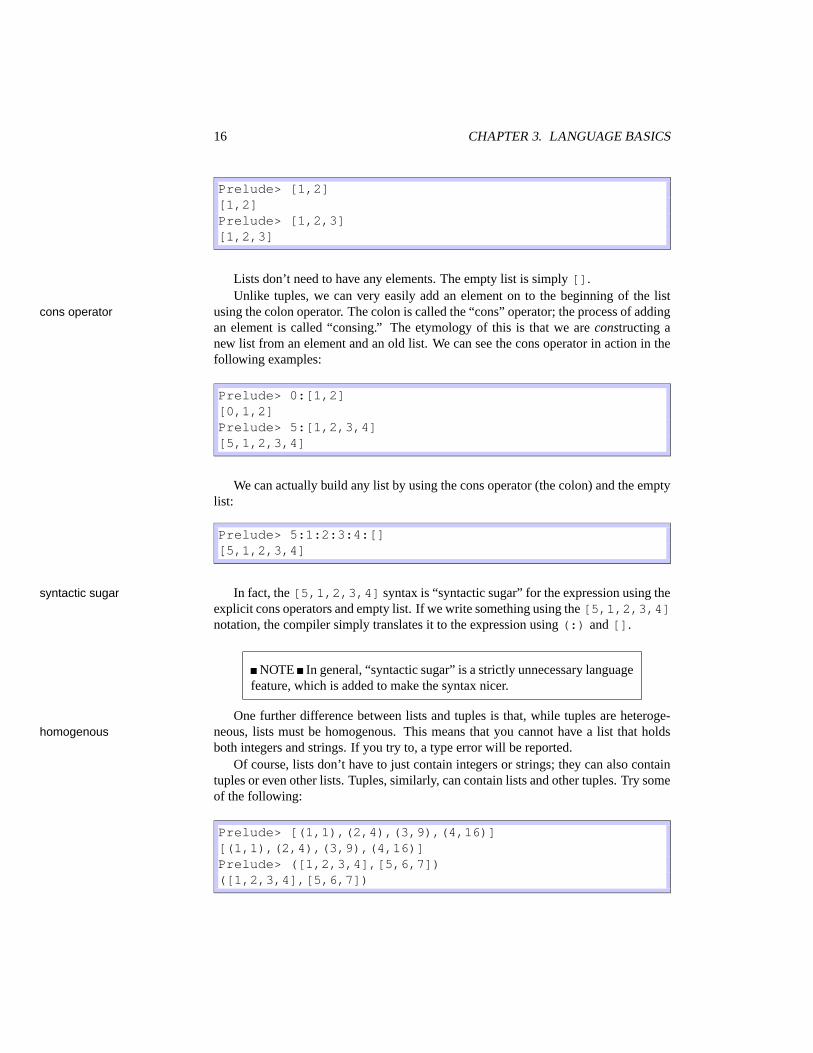
Prelude> [1,2][1,2]Prelude> [1,2,3][1,2,3]
Lists don’t need to have any elements. The empty list is simply [].Unlike tuples, we can very easily add an element on to the beginning of the list
using the colon operator. The colon is called the “cons” operator; the process of addingcons operatoran element is called “consing.” The etymology of this is that we are constructing anew list from an element and an old list. We can see the cons operator in action in thefollowing examples:
Prelude> 0:[1,2][0,1,2]Prelude> 5:[1,2,3,4][5,1,2,3,4]
We can actually build any list by using the cons operator (the colon) and the emptylist:
Prelude> 5:1:2:3:4:[][5,1,2,3,4]
In fact, the [5,1,2,3,4] syntax is “syntactic sugar” for the expression using thesyntactic sugarexplicit cons operators and empty list. If we write something using the [5,1,2,3,4]notation, the compiler simply translates it to the expression using (:) and [].
NOTE In general, “syntactic sugar” is a strictly unnecessary languagefeature, which is added to make the syntax nicer.
One further difference between lists and tuples is that, while tuples are heteroge-neous, lists must be homogenous. This means that you cannot have a list that holdshomogenousboth integers and strings. If you try to, a type error will be reported.
Of course, lists don’t have to just contain integers or strings; they can also containtuples or even other lists. Tuples, similarly, can contain lists and other tuples. Try someof the following:
Prelude> [(1,1),(2,4),(3,9),(4,16)][(1,1),(2,4),(3,9),(4,16)]Prelude> ([1,2,3,4],[5,6,7])([1,2,3,4],[5,6,7])
3.3. LISTS 17
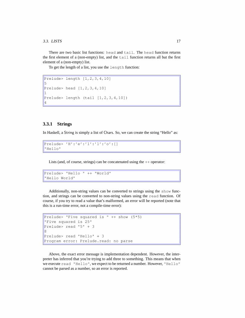
There are two basic list functions: head and tail. The head function returnsthe first element of a (non-empty) list, and the tail function returns all but the firstelement of a (non-empty) list.
To get the length of a list, you use the length function:
Prelude> length [1,2,3,4,10]5Prelude> head [1,2,3,4,10]1Prelude> length (tail [1,2,3,4,10])4
3.3.1 Strings
In Haskell, a String is simply a list of Chars. So, we can create the string “Hello” as:
Prelude> ’H’:’e’:’l’:’l’:’o’:[]"Hello"
Lists (and, of course, strings) can be concatenated using the ++ operator:
Prelude> "Hello " ++ "World""Hello World"
Additionally, non-string values can be converted to strings using the show func-tion, and strings can be converted to non-string values using the read function. Ofcourse, if you try to read a value that’s malformed, an error will be reported (note thatthis is a run-time error, not a compile-time error):
Prelude> "Five squared is " ++ show (5*5)"Five squared is 25"Prelude> read "5" + 38Prelude> read "Hello" + 3Program error: Prelude.read: no parse
Above, the exact error message is implementation dependent. However, the inter-preter has inferred that you’re trying to add three to something. This means that whenwe execute read "Hello", we expect to be returned a number. However, "Hello"cannot be parsed as a number, so an error is reported.
18 CHAPTER 3. LANGUAGE BASICS
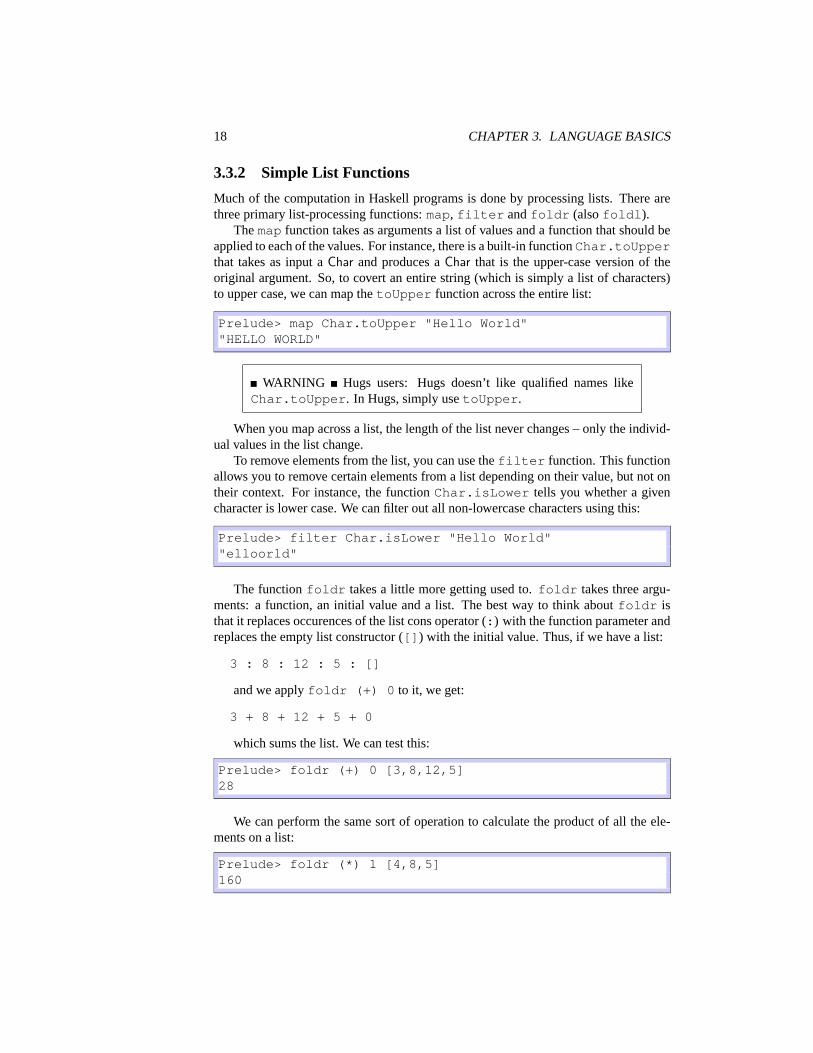
3.3.2 Simple List Functions
Much of the computation in Haskell programs is done by processing lists. There arethree primary list-processing functions: map, filter and foldr (also foldl).
The map function takes as arguments a list of values and a function that should beapplied to each of the values. For instance, there is a built-in function Char.toUpperthat takes as input a Char and produces a Char that is the upper-case version of theoriginal argument. So, to covert an entire string (which is simply a list of characters)to upper case, we can map the toUpper function across the entire list:
Prelude> map Char.toUpper "Hello World""HELLO WORLD"
WARNING Hugs users: Hugs doesn’t like qualified names likeChar.toUpper. In Hugs, simply use toUpper.
When you map across a list, the length of the list never changes – only the individ-ual values in the list change.
To remove elements from the list, you can use the filter function. This functionallows you to remove certain elements from a list depending on their value, but not ontheir context. For instance, the function Char.isLower tells you whether a givencharacter is lower case. We can filter out all non-lowercase characters using this:
Prelude> filter Char.isLower "Hello World""elloorld"
The function foldr takes a little more getting used to. foldr takes three argu-ments: a function, an initial value and a list. The best way to think about foldr isthat it replaces occurences of the list cons operator (:) with the function parameter andreplaces the empty list constructor ([]) with the initial value. Thus, if we have a list:
3 : 8 : 12 : 5 : []
and we apply foldr (+) 0 to it, we get:
3 + 8 + 12 + 5 + 0
which sums the list. We can test this:
Prelude> foldr (+) 0 [3,8,12,5]28
We can perform the same sort of operation to calculate the product of all the ele-ments on a list:
Prelude> foldr (*) 1 [4,8,5]160

3.3. LISTS 19
We said earlier that folding is like replacing (:) with a particular function and ([])with an initial element. This raises a question as to what happens when the functionisn’t associative (a function (·) is associative if a · (b · c) = (a · b) · c). When we write4 · 8 · 5 · 1, we need to specify where to put the parentheses. Namely, do we mean((4 · 8) · 5) · 1 or 4 · (8 · ((5 · 1))? foldr assumes the function is right-associative (i.e.,the correct bracketing is the latter). Thus, when we use it on a non-associtive function(like minus), we can see the effect:
Prelude> foldr (-) 1 [4,8,5]0
The exact derivation of this looks something like:
foldr (-) 1 [4,8,5]==> 4 - (foldr (-) 1 [8,5])==> 4 - (8 - foldr (-) 1 [5])==> 4 - (8 - (5 - foldr (-) 1 []))==> 4 - (8 - (5 - 1))==> 4 - (8 - 4)==> 4 - 4==> 0
The foldl function goes the other way and effectively produces the oppositebracketing. foldl looks the same when applied, so we could have done summingjust as well with foldl:
Prelude> foldl (+) 0 [3,8,12,5]28
However, we get different results when using the non-associative function minus:
Prelude> foldl (-) 1 [4,8,5]-16
This is because foldl uses the opposite bracketing. The way it accomplishes thisis essentially by going all the way down the list, taking the last element and combiningit with the initial value via the provided function. It then takes the second-to-last ele-ment in the list and combines it to this new value. It does so until there is no more listleft.
The derivation here proceeds in the opposite fashion:
foldl (-) 1 [4,8,5]==> foldl (-) (1 - 4) [8,5]==> foldl (-) ((1 - 4) - 8) [5]==> foldl (-) (((1 - 4) - 8) - 5) []

20 CHAPTER 3. LANGUAGE BASICS
==> ((1 - 4) - 8) - 5==> ((-3) - 8) - 5==> (-11) - 5==> -16
Note that once the foldl goes away, the parenthesization is exactly the oppositeof the foldr.
NOTE foldl is often more efficient than foldr for reasons thatwe will discuss in Section 7.8. However, foldr can work on infinitelists, while foldl cannot. This is because before foldl does any-thing, it has to go to the end of the list. On the other hand, foldrstarts producing output immediately. For instance, foldr (:) [][1,2,3,4,5] simply returns the same list. Even if the list were in-finite, it would produce output. A similar function using foldl wouldfail to produce any output.
If this discussion of the folding functions is still somewhat unclear, that’s okay.We’ll discuss them further in Section 7.8.
ExercisesExercise 3.3 Use map to convert a string into a list of booleans, each element in thenew list representing whether or not the original element was a lower-case character.That is, it should take the string “aBCde” and return [True,False,False,True,True].
Exercise 3.4 Use the functions mentioned in this section (you will need two of them)to compute the number of lower-case letters in a string. For instance, on “aBCde” itshould return 3.
Exercise 3.5 We’ve seen how to calculate sums and products using folding functions.Given that the function max returns the maximum of two numbers, write a functionusing a fold that will return the maximum value in a list (and zero if the list is empty).So, when applied to [5,10,2,8,1] it will return 10. Assume that the values in the list arealways ≥ 0. Explain to yourself why it works.
Exercise 3.6 Write a function that takes a list of pairs of length at least 2 and re-turns the first component of the second element in the list. So, when provided with[(5,’b’),(1,’c’),(6,’a’)], it will return 1.
3.4 Source Code Files
As programmers, we don’t want to simply evaluate small expressions like these – wewant to sit down, write code in our editor of choice, save it and then use it.
We already saw in Sections 2.2 and 2.3 how to write a Hello World program andhow to compile it. Here, we show how to use functions defined in a source-code filein the interactive environment. To do this, create a file called Test.hs and enter thefollowing code:

3.4. SOURCE CODE FILES 21
module Testwhere
x = 5y = (6, "Hello")z = x * fst y
This is a very simple “program” written in Haskell. It defines a module called“Test” (in general module names should match file names; see Section 6 for more onthis). In this module, there are three definitions: x, y and z. Once you’ve writtenand saved this file, in the directory in which you saved it, load this in your favoriteinterpreter, by executing either of the following:
% hugs Test.hs% ghci Test.hs
This will start Hugs or GHCi, respectively, and load the file. Alternatively, if youalready have one of them loaded, you can use the “:load” command (or just “:l”) toload a module, as:
Prelude> :l Test.hs...Test>
Between the first and last line, the interpreter will print various data to explain whatit is doing. If any errors appear, you probably mistyped something in the file; doublecheck and then try again.
You’ll notice that where it used to say “Prelude” it now says “Test.” That meansthat Test is the current module. You’re probably thinking that “Prelude” must also bea module. Exactly correct. The Prelude module (usually simply referred to as “thePrelude”) is always loaded and contains the standard definitions (for instance, the (:) the Preludeoperator for lists, or (+) or (*), fst, snd and so on).
Now that we’ve loaded Test, we can use things that were defined in it. For example:
Test> x5Test> y(6,"Hello")Test> z30
Perfect, just as we expected!One final issue regarding how to compile programs to stand-alone executables re-
mains. In order for a program to be an executable, it must have the module name

22 CHAPTER 3. LANGUAGE BASICS
“Main” and must contain a function called main. So, if you go in to Test.hs and re-name it to “Main” (change the line that reads module Test to module Main), wesimply need to add a main function. Try this:
main = putStrLn "Hello World"
Now, save the file, and compile it (refer back to Section 2 for information on howto do this for your compiler). For example, in GHC, you would say:
% ghc --make Test.hs -o test
NOTE For Windows, it would be “-o test.exe”
This will create a file called “test” (or on Windows, “test.exe”) that you can thenrun.
% ./testHello World
NOTE Or, on Windows:
C:\> test.exeHello World
3.5 Functions
Now that we’ve seen how to write code in a file, we can start writing functions. As youmight have expected, functions are central to Haskell, as it is a functional language.This means that the evaluation of a program is simply the evaluation of a function.
We can write a simple function to square a number and enter it into our Test.hsfile. We might define this as follows:
square x = x * x
In this function definition, we say that we’re defining a function square that takesone argument (aka parameter), which we call x. We then say that the value of squarex is equal to x * x.
Haskell also supports standard conditional expressions. For instance, we coulddefine a function that returns −1 if its argument is less than 0; 0 if its argument is 0;and 1 if its argument is greater than 0 (this is called the signum function):

3.5. FUNCTIONS 23
signum x =if x < 0
then -1else if x > 0then 1else 0
You can experiment with this as:
Test> signum 51Test> signum 00Test> signum (5-10)-1Test> signum (-1)-1
Note that the parenthesis around “-1” in the last example are required; if missing,the system will think you are trying to subtract the value “1” from the value “signum,”which is illtyped.
The if/then/else construct in Haskell is very similar to that of most other program-ming languages; however, you must have both a then and an else clause. It evaluates if/then/elsethe condition (in this case x < 0 and, if this evaluates to True, it evaluates the thencondition; if the condition evaluated to False, it evaluates the else condition).
You can test this program by editing the file and loading it back into your interpreter.If Test is already the current module, instead of typing :l Test.hs again, you cansimply type :reload or just :r to reload the current file. This is usually much faster.
Haskell, like many other languages, also supports case constructions. These are case/ofused when there are multiple values that you want to check against (case expressionsare actually quite a bit more powerful than this – see Section 7.4 for all of then details).
Suppose we wanted to define a function that had a value of 1 if its argument were0; a value of 5 if its argument were 1; a value of 2 if its argument were 2; and a value of−1 in all other instances. Writing this function using if statements would be long andvery unreadable; so we write it using a case statement as follows (we call this functionf):
f x =case x of
0 -> 11 -> 52 -> 2_ -> -1

24 CHAPTER 3. LANGUAGE BASICS
In this program, we’re defining f to take an argument x and then inspect the valueof x. If it matches 0, the value of f is 1. If it matches 1, the value of f is 5. If it maches2, then the value of f is 2; and if it hasn’t matched anything by that point, the value off is −1 (the underscore can be thought of as a “wildcard” – it will match anything) .wildcard
The indentation here is important. Haskell uses a system called “layout” to struc-ture its code (the programming language Python uses a similar system). The layoutsystem allows you to write code without the explicit semicolons and braces that otherlanguages like C and Java require.
WARNING Because whitespace matters in Haskell, you need to becareful about whether you are using tabs or spaces. If you can configureyour editor to never use tabs, that’s probably better. If not, make sureyour tabs are always 8 spaces long, or you’re likely to run in to problems.
The general rule for layout is that an open-brace is inserted after the keywordswhere, let, do and of, and the column position at which the next command appearsis remembered. From then on, a semicolon is inserted before every new line that isindented the same amount. If a following line is indented less, a close-brace is inserted.This may sound complicated, but if you follow the general rule of indenting after eachof those keywords, you’ll never have to remember it (see Section 7.11 for a morecomplete discussion of layout).
Some people prefer not to use layout and write the braces and semicolons explicitly.This is perfectly acceptable. In this style, the above function might look like:
f x = case x of{ 0 -> 1 ; 1 -> 5 ; 2 -> 2 ; _ -> 1 }
Of course, if you write the braces and semicolons explicitly, you’re free to structurethe code as you wish. The following is also equally valid:
f x =case x of { 0 -> 1 ;1 -> 5 ; 2 -> 2
; _ -> 1 }
However, structuring your code like this only serves to make it unreadable (in thiscase).
Functions can also be defined piece-wise, meaning that you can write one versionof your function for certain parameters and then another version for other parameters.For instance, the above function f could also be written as:
f 0 = 1f 1 = 5f 2 = 2f _ = -1

3.5. FUNCTIONS 25
Here, the order is important. If we had put the last line first, it would have matchedevery argument, and f would return -1, regardless of its argument (most compilerswill warn you about this, though, saying something about overlapping patterns). If wehad not included this last line, f would produce an error if anything other than 0, 1 or2 were applied to it (most compilers will warn you about this, too, saying somethingabout incomplete patterns). This style of piece-wise definition is very popular and willbe used quite frequently throughout this tutorial. These two definitions of f are actuallyequivalent – this piece-wise version is translated into the case expression.
More complicated functions can be built from simpler functions using functioncomposition. Function composition is simply taking the result of the application of onefunction and using that as an argument for another. We’ve already seen this way backin arithmetic (Section 3.1), when we wrote 5*4+3. In this, we were evaluating 5 ∗ 4and then applying +3 to the result. We can do the same thing with our square and ffunctions:
Test> square (f 1)25Test> square (f 2)4Test> f (square 1)5Test> f (square 2)-1
The result of each of these function applications is fairly straightforward. Theparentheses around the inner function are necessary; otherwise, in the first line, theinterpreter would think that you were trying to get the value of “square f,” whichhas no meaning. Function application like this is fairly standard in most programminglanguages. There is another, more mathematically oriented, way to express functioncomposition, using the (.) (just a single period) function. This (.) function is supposedto look like the (◦) operator in mathematics.
NOTE In mathematics we write f ◦ g to mean “f following g,” inHaskell we write f . g also to mean “f following g.”The meaning of f ◦ g is simply that (f ◦ g)(x) = f(g(x)). That is,applying the value x to the function f ◦ g is the same as applying it to g,taking the result, and then applying that to f .
The (.) function (called the function composition function), takes two functions function compositionand makes them in to one. For instance, if we write (square . f), this means thatit creates a new function that takes an argument, applies f to that argument and thenapplies square to the result. Conversely, (f . square) means that it createsa new function that takes an argument, applies square to that argument and thenapplies f to the result. We can see this by testing it as before:
Test> (square . f) 125

26 CHAPTER 3. LANGUAGE BASICS
Test> (square . f) 24Test> (f . square) 15Test> (f . square) 2-1
Here, we must enclose the function composition in parentheses; otherwise, theHaskell compiler will think we’re trying to compose square with the value f 1 inthe first line, which makes no sense since f 1 isn’t even a function.
It would probably be wise to take a little time-out to look at some of the functionsthat are defined in the Prelude. Undoubtedly, at some point, you will accidentallyrewrite some already-existing function (I’ve done it more times than I can count), butif we can keep this to a minimum, that would save a lot of time. Here are some simplefunctions, some of which we’ve already seen:
sqrt the square root functionid the identity function: id x = xfst extracts the first element from a pairsnd extracts the second element from a pairnull tells you whether or not a list is emptyhead returns the first element on a non-empty listtail returns everything but the first element of a non-empty list++ concatenates two lists== checks to see if two elements are equal/= checks to see if two elements are unequal
Here, we show example usages of each of these functions:
Prelude> sqrt 21.41421Prelude> id "hello""hello"Prelude> id 55Prelude> fst (5,2)5Prelude> snd (5,2)2Prelude> null []TruePrelude> null [1,2,3,4]FalsePrelude> head [1,2,3,4]1Prelude> tail [1,2,3,4][2,3,4]Prelude> [1,2,3] ++ [4,5,6]

3.5. FUNCTIONS 27
[1,2,3,4,5,6]Prelude> [1,2,3] == [1,2,3]TruePrelude> ’a’ /= ’b’TruePrelude> head []
Program error: {head []}
We can see that applying head to an empty list gives an error (the exact errormessage depends on whether you’re using GHCi or Hugs – the shown error message isfrom Hugs).
3.5.1 Let Bindings
Often we wish to provide local declarations for use in our functions. For instance, ifyou remember back to your grade school mathematics courses, the following equationis used to find the roots (zeros) of a polynomial of the form ax2 + bx + c = 0: x =(−b ±
√b2 − 4ac)/2a. We could write the following function to compute the two
values of x:
roots a b c =((-b + sqrt(b*b - 4*a*c)) / (2*a),(-b - sqrt(b*b - 4*a*c)) / (2*a))
To remedy this problem, Haskell allows for local bindings. That is, we can createvalues inside of a function that only that function can see. For instance, we couldcreate a local binding for sqrt(b*b-4*a*c) and call it, say, det and then use thatin both places where sqrt(b*b - 4*a*c) occurred. We can do this using a let/indeclaration:
roots a b c =let det = sqrt (b*b - 4*a*c)in ((-b + det) / (2*a),
(-b - det) / (2*a))
In fact, you can provide multiple declarations inside a let. Just make sure they’reindented the same amount, or you will have layout problems:
roots a b c =let det = sqrt (b*b - 4*a*c)
twice_a = 2*ain ((-b + det) / twice_a,
(-b - det) / twice_a)

28 CHAPTER 3. LANGUAGE BASICS
3.5.2 Infix
Infix functions are ones that are composed of symbols, rather than letters. For instance,(+), (*), (++) are all infix functions. You can use them in non-infix mode byenclosing them in parentheses. Hence, the two following expressions are the same:
Prelude> 5 + 1015Prelude> (+) 5 1015
Similarly, non-infix functions (like map) can be made infix by enclosing them inbackquotes (the ticks on the tilde key on American keyboards):
Prelude> map Char.toUpper "Hello World""HELLO WORLD"Prelude> Char.toUpper ‘map‘ "Hello World""HELLO WORLD"
WARNING Hugs users: Hugs doesn’t like qualified names likeChar.toUpper. In Hugs, simply use toUpper.
3.6 Comments
There are two types of comments in Haskell: line comments and block comments.Line comments begin with the token -- and extend until the end of the line. Blockcomments begin with {- and extend to a corresponding -}. Block comments can benested.
NOTE The -- in Haskell corresponds to // in C++ or Java, and {-and -} correspond to /* and */.
Comments are used to explain your program in English and are completely ignoredby compilers and interpreters. For example:
module Test2where
main =putStrLn "Hello World" -- write a string
-- to the screen
{- f is a function which takes an integer andproduces integer. {- this is an embedded
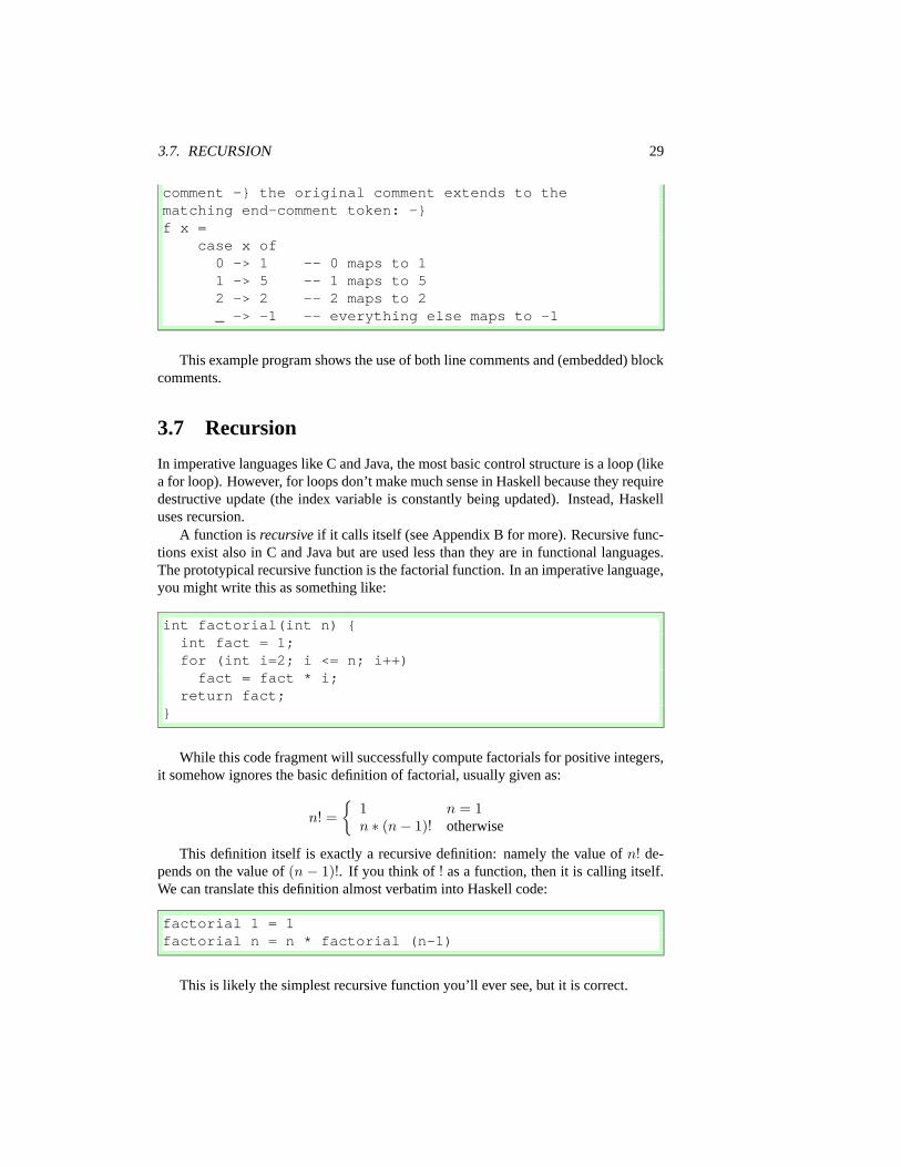
3.7. RECURSION 29
comment -} the original comment extends to thematching end-comment token: -}f x =
case x of0 -> 1 -- 0 maps to 11 -> 5 -- 1 maps to 52 -> 2 -- 2 maps to 2_ -> -1 -- everything else maps to -1
This example program shows the use of both line comments and (embedded) blockcomments.
3.7 Recursion
In imperative languages like C and Java, the most basic control structure is a loop (likea for loop). However, for loops don’t make much sense in Haskell because they requiredestructive update (the index variable is constantly being updated). Instead, Haskelluses recursion.
A function is recursive if it calls itself (see Appendix B for more). Recursive func-tions exist also in C and Java but are used less than they are in functional languages.The prototypical recursive function is the factorial function. In an imperative language,you might write this as something like:
int factorial(int n) {int fact = 1;for (int i=2; i <= n; i++)fact = fact * i;
return fact;}
While this code fragment will successfully compute factorials for positive integers,it somehow ignores the basic definition of factorial, usually given as:
n! =
{
1 n = 1n ∗ (n − 1)! otherwise
This definition itself is exactly a recursive definition: namely the value of n! de-pends on the value of (n − 1)!. If you think of ! as a function, then it is calling itself.We can translate this definition almost verbatim into Haskell code:
factorial 1 = 1factorial n = n * factorial (n-1)
This is likely the simplest recursive function you’ll ever see, but it is correct.

30 CHAPTER 3. LANGUAGE BASICS
NOTE Of course, an imperative recursive version could be written:
int factorial(int n) {if (n == 1)return 1;
elsereturn n * factorial(n-1);
}
but this is likely to be much slower than the loop version in C.
Recursion can be a difficult thing to master. It is completely analogous to theconcept of induction in mathematics (see Chapter B for a more formal treatment ofthis). However, usually a problem can be thought of as having one or more base casesand one or more recursive-cases. In the case of factorial, there is one base case(when n = 1) and one recursive case (when n > 1). For designing your own recusivealgorithms, it is often useful to try to differentiate these two cases.
Turning now to the task of exponentiation, suppose that we have two positive in-tegers a and b, and that we want to calculate ab. This problem has a single base case:namely when b is 1. The recursive case is when b > 1. We can write a general form as:
ab =
{
a b = 1a ∗ ab−1 otherwise
Again, this translates directly into Haskell code:
exponent a 1 = aexponent a b = a * exponent a (b-1)
Just as we can define recursive functions on integers, so can we define recursivefunctions on lists. In this case, usually the base case is the empty list [], and therecursive case is a cons list (i.e., a value consed on to another list).
Consider the task of calculating the length of a list. We can again break this downinto two cases: either we have an empty list or we have a non-empty list. Clearly thelength of an empty list is zero. Furthermore, if we have a cons list, then the length ofthis list is just the length of its tail plus one. Thus, we can define a length function as:
my_length [] = 0my_length (x:xs) = 1 + my_length xs
NOTE Whenever we provide alternative definitions for standardHaskell functions, we prefix them with my so the compiler doesn’t be-come confused.

3.8. INTERACTIVITY 31
Similarly, we can consider the filter function. Again, the base case is the emptylist, and the recursive case is a cons list. However, this time, we’re choosing whetherto keep an element, depending on whether or not a particular predicate holds. We candefine the filter function as:
my_filter p [] = []my_filter p (x:xs) =if p xthen x : my_filter p xselse my_filter p xs
In this code, when presented with an empty list, we simply return an empty list.This is because filter cannot add elements; it can only remove them.
When presented with a list of the form (x:xs), we need to decide whether or notto keep the value x. To do this, we use an if statement and the predicate p. If p x istrue, then we return a list that begins with x followed by the result of filtering the tailof the list. If p x is false, then we exclude x and return the result of filtering the tail ofthe list.
We can also define map and both fold functions using explicit recursion. See theexercises for the definition of map and Chapter 7 for the folds.
ExercisesExercise 3.7 The fibonacci sequence is defined by:
Fn =
{
1 n = 1 or n = 2Fn−2 + Fn−1 otherwise
Write a recursive function fib that takes a positive integer n as a parameter andcalculates Fn.
Exercise 3.8 Define a recursive function mult that takes two positive integers a andb and returns a*b, but only uses addition (i.e., no fair just using multiplication). Beginby making a mathematical definition in the style of the previous exercise and the rest ofthis section.
Exercise 3.9 Define a recursive function my map that behaves identically to the stan-dard function map.
3.8 Interactivity
If you are familiar with books on other (imperative) languages, you might be wonder-ing why you haven’t seen many of the standard programs written in tutorials of otherlanguages (like ones that ask the user for his name and then says “Hi” to him by name).The reason for this is simple: Being a pure functional language, it is not entirely clearhow one should handle operations like user input.
32 CHAPTER 3. LANGUAGE BASICS
After all, suppose you have a function that reads a string from the keyboard. Ifyou call this function twice, and the user types something the first time and somethingelse the second time, then you no longer have a function, since it would return twodifferent values. The solution to this was found in the depths of category theory, abranch of formal mathematics: monads. We’re not yet ready to talk about monadsmonadsformally, but for now, think of them simply as a convenient way to express operationslike input/output. We’ll discuss them in this context much more in Chapter 5 and thendiscuss monads for monads’ sake in Chapter 9.
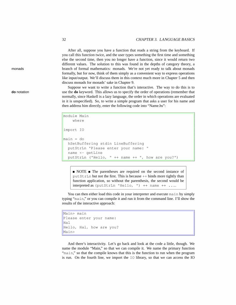
Suppose we want to write a function that’s interactive. The way to do this is touse the do keyword. This allows us to specify the order of operations (remember thatdo notationnormally, since Haskell is a lazy language, the order in which operations are evaluatedin it is unspecified). So, to write a simple program that asks a user for his name andthen address him directly, enter the following code into “Name.hs”:
module Mainwhere
import IO
main = dohSetBuffering stdin LineBufferingputStrLn "Please enter your name: "name <- getLineputStrLn ("Hello, " ++ name ++ ", how are you?")
NOTE The parentheses are required on the second instance ofputStrLn but not the first. This is because ++ binds more tightly thanfunction application, so without the parenthesis, the second would beinterpreted as (putStrLn "Hello, ") ++ name ++ ....
You can then either load this code in your interpreter and execute main by simplytyping “main,” or you can compile it and run it from the command line. I’ll show theresults of the interactive approach:
Main> mainPlease enter your name:HalHello, Hal, how are you?Main>
And there’s interactivity. Let’s go back and look at the code a little, though. Wename the module “Main,” so that we can compile it. We name the primary function“main,” so that the compile knows that this is the function to run when the programis run. On the fourth line, we import the IO library, so that we can access the IO
3.8. INTERACTIVITY 33
functions. On the seventh line, we start with do, telling Haskell that we’re executing asequence of commands.
The first command is hSetBuffering stdin LineBuffering, which youshould probably ignore for now (incidentally, this is only required by GHC – in Hugsyou can get by without it). The necessity for this is because, when GHC reads input, itexpects to read it in rather large blocks. A typical person’s name is nowhere near largeenough to fill this block. Thus, when we try to read from stdin, it waits until it’sgotten a whole block. We want to get rid of this, so we tell it to use LineBufferinginstead of block buffering.
The next command is putStrLn, which prints a string to the screen. On theninth line, we say “name <- getLine.” This would normally be written “name =getLine,” but using the arrow instead of the equal sign shows that getLine isn’ta real function and can return different values. This command means “run the actiongetLine, and store the results in name.”
The last line constructs a string using what we read in the previous line and thenprints it to the screen.
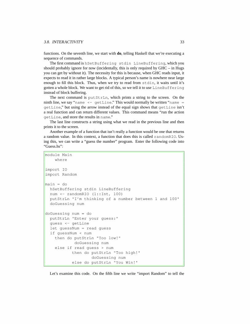
Another example of a function that isn’t really a function would be one that returnsa random value. In this context, a function that does this is called randomRIO. Us-ing this, we can write a “guess the number” program. Enter the following code into“Guess.hs”:
module Mainwhere
import IOimport Random
main = dohSetBuffering stdin LineBufferingnum <- randomRIO (1::Int, 100)putStrLn "I’m thinking of a number between 1 and 100"doGuessing num
doGuessing num = doputStrLn "Enter your guess:"guess <- getLinelet guessNum = read guessif guessNum < numthen do putStrLn "Too low!"
doGuessing numelse if read guess > num
then do putStrLn "Too high!"doGuessing num
else do putStrLn "You Win!"
Let’s examine this code. On the fifth line we write “import Random” to tell the

34 CHAPTER 3. LANGUAGE BASICS
compiler that we’re going to be using some random functions (these aren’t built intothe Prelude). In the first line of main, we ask for a random number in the range(1, 100). We need to write ::Int to tell the compiler that we’re using integers here –not floating point numbers or other numbers. We’ll talk more about this in Section 4.On the next line, we tell the user what’s going on, and then, on the last line of main,we tell the compiler to execute the command doGuessing.
The doGuessing function takes the number the user is trying to guess as anargument. First, it asks the user to guess and then accepts their guess (which is aString) from the keyboard. The if statement checks first to see if their guess is toolow. However, since guess is a string, and num is an integer, we first need to convertguess to an integer by reading it. Since “read guess” is a plain, pure function(and not an IO action), we don’t need to use the <- notation (in fact, we cannot); wesimply bind the value to guessNum. Note that while we’re in do notation, we don’tneed ins for lets.
If they guessed too low, we inform them and then start doGuessing over again.If they didn’t guess too low, we check to see if they guessed too high. If they did,we tell them and start doGuessing again. Otherwise, they didn’t guess too low andthey didn’t guess too high, so they must have gotten it correct. We tell them that theywon and exit. The fact that we exit is implicit in the fact that there are no commandsfollowing this. We don’t need an explicit return () statement.
You can either compile this code or load it into your interpreter, and you will getsomething like:
Main> mainI’m thinking of a number between 1 and 100Enter your guess:50Too low!Enter your guess:75Too low!Enter your guess:85Too high!Enter your guess:80Too high!Enter your guess:78Too low!Enter your guess:79You Win!
The recursive action that we just saw doesn’t actually return a value that we use inany way. In the case when it does, the “obvious” way to write the command is actually

3.8. INTERACTIVITY 35
incorrect. Here, we will give the incorrect version, explain why it is wrong, then givethe correct version.
Let’s say we’re writing a simple program that repeatedly asks the user to type in afew words. If at any point the user enters the empty word (i.e., he just hits enter withouttyping anything), the program prints out everything he’s typed up until that point andthen exits. The primary function (actually, an action) in this program is one that asksthe user for a word, checks to see if it’s empty, and then either continues or ends. Theincorrect formulation of this might look something like:
askForWords = doputStrLn "Please enter a word:"word <- getLineif word == ""then return []else return (word : askForWords)
Before reading ahead, see if you can figure out what is wrong with the above code.The error is on the last line, specifically with the term word : askForWords.
Remeber that when using (:), we are making a list out of an element (in this caseword) and another list (in this case, askForWords). However, askForWords isnot a list; it is an action that, when run, will produce a list. That means that before wecan attach anything to the front, we need to run the action and take the result. In thiscase, we want to do something like:
askForWords = doputStrLn "Please enter a word:"word <- getLineif word == ""then return []else do
rest <- askForWordsreturn (word : rest)
Here, we first run askForWords, take the result and store it in the variable rest.Then, we return the list created from word and rest.
By now, you should have a good understanding of how to write simple functions,compile them, test functions and programs in the interactive environment, and manip-ulate lists.
ExercisesExercise 3.10 Write a program that will repeatedly ask the user for numbers until shetypes in zero, at which point it will tell her the sum of all the numbers, the product ofall the numbers, and, for each number, its factorial. For instance, a session might looklike:

36 CHAPTER 3. LANGUAGE BASICS
Give me a number (or 0 to stop):5Give me a number (or 0 to stop):8Give me a number (or 0 to stop):2Give me a number (or 0 to stop):0The sum is 15The product is 805 factorial is 1208 factorial is 403202 factorial is 2
Hint: write an IO action that reads a number and, if it’s zero, returns the empty list. Ifit’s not zero, it recurses itself and then makes a list out of the number it just read andthe result of the recursive call.

Chapter 4
Type Basics
Haskell uses a system of static type checking. This means that every expression inHaskell is assigned a type. For instance ’a’ would have type Char, for “character.”Then, if you have a function which expects an argument of a certain type and you giveit the wrong type, a compile-time error will be generated (that is, you will not be ableto compile the program). This vastly reduces the number of bugs that can creep intoyour program.
Furthermore, Haskell uses a system of type inference. This means that you don’teven need to specify the type of expressions. For comparison, in C, when you definea variable, you need to specify its type (for instance, int, char, etc.). In Haskell, youneedn’t do this – the type will be inferred from context.
NOTE If you want, you certainly are allowed to explicitely specifythe type of an expression; this often helps debugging. In fact, it is some-times considered good style to explicitly specify the types of outermostfunctions.
Both Hugs and GHCi allow you to apply type inference to an expression to find itstype. This is done by using the :t command. For instance, start up your favorite shelland try the following:
Prelude> :t ’c’’c’ :: Char
This tells us that the expression ’c’ has type Char (the double colon :: is usedthroughout Haskell to specify types).
4.1 Simple Types
There are a slew of built-in types, including Int (for integers, both positive and neg-ative), Double (for floating point numbers), Char (for single characters), String (for
37

38 CHAPTER 4. TYPE BASICS
strings), and others. We have already seen an expression of type Char; let’s examimeone of type String:
Prelude> :t "Hello""Hello" :: String
You can also enter more complicated expressions, for instance, a test of equality:
Prelude> :t ’a’ == ’b’’a’ == ’b’ :: Bool
You should note than even though this expression is false, it still has a type, namelythe type Bool.
NOTE Bool is short for Boolean (usually pronounced “boo-lee-uhn”,though I’ve heard “boo-leen” once or twice) and has two possible values:True and False.
You can observe the process of type checking and type inference by trying to getthe shell to give you the type of an ill-typed expression. For instance, the equalityoperator requires that the type of both of its arguments are of the same type. We cansee that Char and String are of different types by trying to compare a character to astring:
Prelude> :t ’a’ == "a"ERROR - Type error in application*** Expression : ’a’ == "a"*** Term : ’a’*** Type : Char*** Does not match : [Char]
The first line of the error (the line containing “Expression”) tells us the expressionin which the type error occured. The second line tells us which part of this expressionis ill-typed. The third line tells us the inferred type of this term and the fourth linetells us what it needs to have matched. In this case, it says that type type Char doesn’tmatch the type [Char] (a list a characters – a string in Haskell is represented as a list ofcharacters).
As mentioned before, you can explicitely specify the type of an expression usingthe :: operator. For instance, instead of ”a” in the previous example, we could havewritten (”a”::String). In this case, this has no effect since there’s only one possibleinterpretation of ”a”. However, consider the case of numbers. You can try:
Prelude> :t 5 :: Int5 :: IntPrelude> :t 5 :: Double5 :: Double

4.2. POLYMORPHIC TYPES 39
Here, we can see that the number 5 can be instantiated as either an Int our a Double.What if we don’t specify the type?
Prelude> :t 55 :: Num a => a
Not quite what you expected? What this means, briefly, is that if some type a isan instance of the Num class, then type type of the expression 5 can be of type a.If that made no sense, that’s okay for now. In Section 4.3 we talk extensively abouttype classes (which is what this is). The way to read this, though, is to say “a being aninstance of Num implies a.”
ExercisesExercise 4.1 Figure out for yourself, and then verify the types of the following expres-sions, if they have a type. Also note if the expression is a type error:
1. ’h’:’e’:’l’:’l’:’o’:[]
2. [5,’a’]
3. (5,’a’)
4. (5::Int) + 10
5. (5::Int) + (10::Double)
4.2 Polymorphic Types
Haskell employs a polymorhpic type system. This essentially means that you can havetype variables, which we have alluded to before. For instance, note that a function liketail doesn’t care what the elements in the list are:
Prelude> tail [5,6,7,8,9][6,7,8,9]Prelude> tail "hello""ello"Prelude> tail ["the","man","is","happy"]["man","is","happy"]
This is possible because tail has a polymorphic type: [α] → [α]. That means itcan take as an argument any list and return a value which is a list of the same type.
The same analysis can explain the type of fst:
Prelude> :t fstforall a b . (a,b) -> a

40 CHAPTER 4. TYPE BASICS
Here, GHCi has made explicit the universal quantification of the type values. Thatis, it is saying that for all types a and b, fst is a function from (a, b) to a.
ExercisesExercise 4.2 Figure out for yourself, and then verify the types of the following expres-sions, if they have a type. Also note if the expression is a type error:
1. snd
2. head
3. null
4. head . tail
5. head . head
4.3 Type Classes
We saw last section some strange typing having to do with the number five. Before wedelve too deeply into the subject of type classes, let’s take a step back and see some ofthe motivation.
4.3.1 Motivation
In many languages (C++, Java, etc.), there exists a system of overloading. That is,a function can be written that takes parameters of differing types. For instance, thecannonical example is the equality function. If we want to compare two integers, weshould use an integer comparison; if we want to compare two floating point numbers,we should use a floating point comparison; if we want to compare two characters,we should use a character comparison. In general, if we want to compare two thingswhich have type α, we want to use an α-compare. We call α a type variable since it isa variable whose value is a type.
NOTE In general, type variables will be written using the first part ofthe Greek alphabet: α, β, γ, δ, . . . .
Unfortunately, this presents some problems for static type checking, since the typechecker doesn’t know which types a certain operation (for instance, equality testing)will be defined for. There are as many solutions to this problem as there are staticallytyped languages (perhaps a slight exageration, but not so much so). The one chosenin Haskell is the system of type classes. Whether this is the “correct” solution or the“best” solution of course depends on your application domain. It is, however, the onewe have, so you should learn to love it.

4.3. TYPE CLASSES 41
4.3.2 Equality Testing
Returning to the issue of equality testing, what we want to be able to do is define afunction == (the equality operator) which takes two parameters, each of the same type(call it α), and returns a boolean. But this function may not be defined for every type;just for some. Thus, we associate this function == with a type class, which we callEq. If a specific type α belongs to a certain type class (that is, all functions associatedwith that class are implemented for α), we say that α is an instance of that class. Forinstance, Int is an instance of Eq since equality is defined over integers.
4.3.3 The Num Class
In addition to overloading operators like ==, Haskell has overloaded numeric constants(i.e., 1, 2, 3, etc.). This was done so that when you type in a number like 5, thecompiler is free to say 5 is an integer or floating point number as it sees fit. It definesthe Num class to contain all of these numbers and certain minimal operations overthem (addition, for instance). The basic numeric types (Int, Double) are defined to beinstances of Num.
We have only skimmed the surface of the power (and complexity) of type classeshere. There will be much more discussion of them in Section 8.4, but we need somemore background before we can get there. Before we do that, we need to talk a littlemore about functions.
4.3.4 The Show Class
Another of the standard classes in Haskell is the Show class. Types which are mem-bers of the Show class have functions which convert values of that type to a string.This function is called show. For instance show applied to the integer 5 is the string“5”; show applied to the character ’a’ is the three-character string “’a”’ (the first andlast characters are apostrophes). show applied to a string simply puts quotes around it.You can test this in the interpreter:
Prelude> show 5"5"Prelude> show ’a’"’a’"Prelude> show "Hello World""\"Hello World\""
NOTE The reason the backslashes appear in the last line is becausethe interior quotes are “escaped”, meaning that they are part of the string,not part of the interpreter printing the value. The actual string doesn’tcontain the backslashes.
Some types are note instances of Show; functions for example. If you try to show afunction (like sqrt), the compiler or interpreter will give you some cryptic error mes-

42 CHAPTER 4. TYPE BASICS
sage, complaining about a missing instance declaration or an illegal class constraint.
4.4 Function Types
In Haskell, functions are first class values, meaning that just as 1 or ’c’ are valueswhich have a type, so are functions like square or ++. Before we talk too much aboutfunctions, we need to make a short diversion into very theoretical computer science(don’t worry, it won’t be too painful) and talk about the lambda calculus.
4.4.1 Lambda Calculus
The name “Lambda Calculus”, while perhaps daunting, describes a fairly simple sys-tem for representing functions. The way we would write a squaring function in lambdacalculus is: λx.x∗x, which means that we take a value, which we will call x (that’s what“λx. means) and then multiply it by itself. The λ is called “lambda abstraction.” Ingeneral, lambdas can only have one parameter. If we want to write a function that takestwo numbers, doubles the first and adds it to the second, we would write: λxλy.2∗x+y.When we apply a value to a lambda expression, we remove the outermost λ and replaceevery occurrence of the lambda variable with the value. For instance, if we evaluate(λx.x ∗ x)5, we remove the lambda and replace every occurrence of x with 5, yielding(5 ∗ 5) which is 25.
In fact, Haskell is largely based on an extension of the lambda calculus, and thesetwo expressions can be written directly in Haskell (we simply replace the λ with abackslash and the . with an arrow; also we don’t need to repeat the lambdas; and, ofcourse, in Haskell we have to give them names if we’re defining functions):
square = \x -> x*xf = \x y -> 2*x + y
You can also evaluate lambda expressions in your interactive shell:
Prelude> (\x -> x*x) 525Prelude> (\x y -> 2*x + y) 5 414
We can see in the second example that we need to give the lambda abstraction twoarguments, one corresponding to x and the other corresponding to y.
4.4.2 Higher-Order Types
“Higher-Order Types” is the name given to functions. The type given to functions mim-icks the lambda calculus representation of the functions. For instance, the definition ofsquare gives λx.x ∗ x. To get the type of this, we first ask ourselves what the type of x

4.4. FUNCTION TYPES 43
is. Say we decide x is an Int. Then, we notice that the function square takes an Int
and produces a value x*x. We know that when we multiply two Ints together, we getanother Int, so the type of the results of square is also an Int. Thus, we say the typeof square is Int → Int.
We can apply a similar analysis to the function f above. The value of this function(remember, functions are values) is something which takes a value x and given thatvalue, produces a new value, which takes a value y and produces 2*x+y. For instance,if we take f and apply only one number to it, we get (λxλy.2x + y)5 which becomesour new value λy.2(5) + y, where all occurances of x have been replaced with theapplied value, 5.
So we know that f takes an Int and produces a value of some type, of which we’renot sure. But we know the type of this value is the type of λy.2(5) + y. We ap-ply the above analysis and find out that this expression has type Int → Int. Thus, ftakes an Int and produces something which has type Int → Int. So the type of f isInt → (Int → Int).
NOTE The parentheses are not necessary; in function types, if youhave α → β → γ it is assume that β → γ is grouped. If you want theother way, with α → β grouped, you need to put parentheses aroundthem.
This isn’t entirely accurate. As we saw before, numbers like 5 aren’t really of typeInt, they are of type Num a ⇒ a.
We can easily find the type of Prelude functions using “:t” as before:
Prelude> :t headhead :: [a] -> aPrelude> :t tailtail :: [a] -> [a]Prelude> :t nullnull :: [a] -> BoolPrelude> :t fstfst :: (a,b) -> aPrelude> :t sndsnd :: (a,b) -> b
We read this as: “head” is a function that takes a list containing values of type “a”and gives back a value of type “a”; “tail” takes a list of “a”s and gives back another listof “a”s; “null” takes a list of “a”s and gives back a boolean; “fst” takes a pair of type“(a,b)” and gives back something of type “a”, and so on.
NOTE Saying that the type of fst is (a, b) → a does not necessarilymean that it simply gives back the first element; it only means that itgives back something with the same type as the first element.

44 CHAPTER 4. TYPE BASICS
We can also get the type of operators like + and * and ++ and :; however, in orderto do this we need to put them in parentheses. In general, any function which is usedinfix (meaning in the middle of two arguments rather than before them) must be put inparentheses when getting its type.
Prelude> :t (+)(+) :: Num a => a -> a -> aPrelude> :t (*)(*) :: Num a => a -> a -> aPrelude> :t (++)(++) :: [a] -> [a] -> [a]Prelude> :t (:)(:) :: a -> [a] -> [a]
The types of + and * are the same, and mean that + is a function which, for sometype a which is an instance of Num, takes a value of type a and produces anotherfunction which takes a value of type a and produces a value of type a. In short hand,we might say that + takes two values of type a and produces a value of type a, but thisis less precise.
The type of ++ means, in shorthand, that, for a given type a, ++ takes two lists ofas and produces a new list of as. Similarly, : takes a value of type a and another valueof type [a] (list of as) and produces another value of type [a].
4.4.3 That Pesky IO Type
You might be tempted to try getting the type of a function like putStrLn:
Prelude> :t putStrLnputStrLn :: String -> IO ()Prelude> :t readFilereadFile :: FilePath -> IO String
What in the world is that IO thing? It’s basically Haskell’s way of representingthat these functions aren’t really functions. They’re called “IO Actions” (hence theIO). The immediate question which arises is: okay, so how do I get rid of the IO.In brief, you can’t directly remove it. That is, you cannot write a function with typeIO String → String. The only way to use things with an IO type is to combine themwith other functions using (for example), the do notation.
For example, if you’re reading a file using readFile, presumably you want to dosomething with the string it returns (otherwise, why would you read the file in the firstplace). Suppose you have a function f which takes a String and produces an Int. Youcan’t directly apply f to the result of readFile since the input to f is String and theoutput of readFile is IOString and these don’t match. However, you can combinethese as:

4.4. FUNCTION TYPES 45
main = dos <- readFile "somefile"let i = f sputStrLn (show i)
Here, we use the arrow convention to “get the string out of the IO action” and thenapply f to the string (called s). We then, for example, print i to the screen. Note thatthe let here doesn’t have a corresponding in. This is because we are in a do block.Also note that we don’t write i <- f s because f is just a normal function, not anIO action.
4.4.4 Explicit Type Declarations
It is sometimes desirable to explicitly specify the types of some elements or functions,for one (or more) of the following reasons:
• Clarity
• Speed
• Debugging
Some people consider it good software engineering to specify the types of all top-level functions. If nothing else, if you’re trying to compile a program and you get typeerrors that you cannot understand, if you declare the types of some of your functionsexplicitly, it may be easier to figure out where the error is.
Type declarations are written separatly from the function definition. For instance,we could explicitly type the function square as in the following code (an explicitlydeclared type is called a type signature):
square :: Num a => a -> asquare x = x*x
These two lines do not even have to be next to eachother. However, the type that youspecify must match the inferred type of the function definition (or be more specific).In this definition, you could apply square to anything which is an instance of Num:Int, Double, etc. However, if you knew apriori that square were only going to beapplied to value of type Int, you could refine its type as:
square :: Int -> Intsquare x = x*x
Now, you could only apply square to values of type Int. Moreover, with this def-inition, the compiler doesn’t have to generate the general code specified in the original

46 CHAPTER 4. TYPE BASICS
function definition since it knows you will only apply square to Ints, so it may beable to generate faster code.
If you have extensions turned on (“-98” in Hugs or “-fglasgow-exts” in GHC(i)),you can also add a type signature to expressions and not just functions. For instance,you could write:
square (x :: Int) = x*x
which tells the compiler that x is an Int; however, it leaves the compiler aloneto infer the type of the rest of the expression. What is the type of square in thisexample? Make your guess then you can check it either by entering this code into a fileand loading it into your interpreter or by asking for the type of the expression:
Prelude> :t (\(x :: Int) -> x*x)
since this lambda abstraction is equivalent to the above function declaration.
4.4.5 Functional Arguments
In Section 3.3 we saw examples of functions taking other functions as arguments. Forinstance, map took a function to apply to each element in a list, filter took a func-tion that told it which elements of a list to keep, and foldl took a function which toldit how to combine list elements together. As with every other function in Haskell, theseare well-typed.
Let’s first think about the map function. It’s job is to take a list of elements andproduce another list of elements. These two lists don’t necessarily have to have thesame types of elements. So map will take a value of type [a] and produce a value oftype [b]. How does it do this? It uses the user-supplied function to convert. In orderto convert an a to a b, this function must have type a → b. Thus, the type of map is(a → b) → [a] → [b], which you can verify in your interpreter with “:t”.
We can apply the same sort of analysis to filter and discern that it has type(a → Bool) → [a] → [a]. As we presented the foldl function, you might be temptedto give it type (a → a → a) → a → [a] → a, meaning that you take a function whichcombines two as into another one, an initial value of type a, a list of as to produce a finalvalue of type a. In fact, foldl has a more general type: (a → b → a) → a → [b] → a.So it takes a function which turn an a and a b into an a, an initial value of type a and alist of bs. It produces an a.
To see this, we can write a function count which counts how many members of alist satisfy a given constraint. You can of course you filter and length to do this,but we will also do it using foldr:
module Countwhere
import Char

4.5. DATA TYPES 47
count1 p l = length (filter p l)count2 p l = foldr (\x c -> if p x then c+1 else c) 0 l
The functioning of count1 is simple. It filters the list l according to the predicatep, then takes the length of the resulting list. On the other hand, count2 uses the intialvalue (which is an integer) to hold the current count. For each element in the list l,it applies the lambda expression shown. This takes two arguments, c which holds thecurrent count and x which is the current element in the list that we’re looking at. Itchecks to see if p holds about x. If it does, it returns the new value c+1, increasing thecount of elements for which the predicate holds. If it doesn’t, it just returns c, the oldcount.
Exercises
Exercise 4.3 Figure out for yourself, and then verify the types of the following expres-sions, if they have a type. Also note if the expression is a type error:
1. \x -> [x]
2. \x y z -> (x,y:z:[])
3. \x -> x + 5
4. \x -> "hello, world"
5. \x -> x ’a’
6. \x -> x x
7. \x -> x + x
4.5 Data Types
Tuples and lists are nice, common ways to define structured values. However, it isoften desirable to be able to define our own data structures and functions over them.So-called “datatypes” are defined using the data keyword.
4.5.1 Pairs
For instance, a definition of a pair of elements (much like the standard, build-in pairtype) could be:
data Pair a b = Pair a b

48 CHAPTER 4. TYPE BASICS
Let’s walk through this code one word at a time. First we say “data” meaning thatwe’re defining a datatype. We then give the name of the datatype, in this case, “Pair.”The “a” and “b” that follow “Pair” are type parameters, just like the “a” is the type ofthe function map. So up until this point, we’ve said that we’re going to define a datastructure called “Pair” which is parameterized over two types, a and b.
After the equals sign, we specify the constructors of this data type. In this case,there is a single constructor, “Pair” (this doesn’t necessarily have to have the samename as the type, but in this case it seems to make more sense). After this pair, weagain write “a b”, which means that in order to construct a Pair we need two values,one of type a and one of type b.
This definition introduces a function, Pair :: a -> b -> Pair a b thatyou can use to construct Pairs. If you enter this code into a file and load it, you cansee how these are constructed:
Datatypes> :t PairPair :: a -> b -> Pair a bDatatypes> :t Pair ’a’Pair ’a’ :: a -> Pair Char aDatatypes> :t Pair ’a’ "Hello":t Pair ’a’ "Hello"Pair ’a’ "Hello" :: Pair Char [Char]
So, by giving Pair two values, we have completely constructed a value of typePair. We can write functions involving pairs as:
pairFst (Pair x y) = xpairSnd (Pair x y) = y
In this, we’ve used the pattern matching capabilities of Haskell to look at a pairan extract values from it. In the definition of pairFst we take an entire Pair andextract the first element; similarly for pairSnd. We’ll discuss pattern matching inmuch more detail in Section 7.4.
ExercisesExercise 4.4 Write a data type declaration for Triple, a type which contains threeelements, all of different types. Write functions tripleFst, tripleSnd and tripleThrto extract respectively the first, second and third elements.
Exercise 4.5 Write a datatype Quadruple which holds four elements. However, thefirst two elements must be the same type and the last two elements must be the sametype. Write a function firstTwo which returns a list containing the first two elementsand a function lastTwo which returns a list containing the last two elements. Writetype signatures for these functions

4.5. DATA TYPES 49
4.5.2 Multiple Constructors
We have seen an example of the data type with one constructor: Pair. It is alsopossible (and extremely useful) to have multiple constructors.
Let us consider a simple function which searches through a list for an elementsatisfying a given predicate and then returns the first element satisfying that predicate.What should we do if none of the elements in the list satisfy the predicate? A fewoptions are listed below:
• Raise an error
• Loop indefinitely
• Write a check function
• Return the first element
• . . .
Raising an error is certainly an option (see Section 10.1 to see how to do this).The problem is that it is difficult/impossible to recover from such errors. Loopingindefinitely is possible, but not terribly useful. We could write a sister function whichchecks to see if the list contains an element satisfying a predicate and leave it up to theuser to always use this function first. We could return the first element, but this is veryad-hoc and difficult to remember.
The fact that there is no basic option to solve this problem simply means we have tothink about it a little more. What are we trying to do? We’re trying to write a functionwhich might succeed and might not. Furthermore, if it does succeed, it returns somesort of value. Let’s write a datatype:
data Maybe a = Nothing| Just a
This is one of the most common datatypes in Haskell and is defined in the Prelude.Here, we’re saying that there are two possible ways to create something of type
Maybe a. The first is to use the nullary constructor Nothing, which takes no ar-guments (this is what “nullary” means). The second is to use the constructor Just,together with a value of type a.
The Maybe type is useful in all sorts of circumstances. For instance, supposewe want to write a function (like head) which returns the first element of a givenlist. However, we don’t want the program to die if the given list is empty. We canaccomplish this with a function like:
firstElement :: [a] -> Maybe afirstElement [] = NothingfirstElement (x:xs) = Just x

50 CHAPTER 4. TYPE BASICS
The type signature here says that firstElement takes a list of as and producessomething with type Maybe a. In the first line of code, we match against the emptylist []. If this match succeeds (i.e., the list is, in fact, empty), we return Nothing. Ifthe first match fails, then we try to match against x:xs which must succeed. In thiscase, we return Just x.
For our findElement function, we represent failure by the value Nothing andsuccess with value a by Just a. Our function might look something like this:
findElement :: (a -> Bool) -> [a] -> Maybe afindElement p [] = NothingfindElement p (x:xs) =
if p x then Just xelse findElement p xs
The first line here gives the type of the function. In this case, our first argumentis the predicate (and takes an element of type a and returns True if and only if theelement satisfies the predicate); the second argument is a list of as. Our return valueis maybe an a. That is, if the function succeeds, we will return Just a and if not,Nothing.
Another useful datatype is the Either type, defined as:
data Either a b = Left a| Right b
This is a way of expressing alternation. That is, something of type Either a bis either a value of type a (using the Left constructor) or a value of type b (using theRight constructor).
Exercises
Exercise 4.6 Write a datatype Tuple which can hold one, two, three or four elements,depending on the constructor (that is, there should be four constructors, one for eachnumber of arguments). Also provide functions tuple1 through tuple4 which take atuple and return Just the value in that position, or Nothing if the number is invalid(i.e., you ask for the tuple4 on a tuple holding only two elements).
Exercise 4.7 Based on our definition of Tuple from the previous exercise, write afunction which takes a Tuple and returns either the value (if it’s a one-tuple), aHaskell-pair (i.e., (’a’,5)) if it’s a two-tuple, a Haskell-triple if it’s a three-tupleor a Haskell-quadruple if it’s a four-tuple. You will need to use the Either type torepresent this.

4.5. DATA TYPES 51
4.5.3 Recursive Datatypes
We can also define recursive datatypes. These are datatypes whose definitions arebased on themselves. For instance, we could define a list datatype as:
data List a = Nil| Cons a (List a)
In this definition, we have defined what it means to be of type List a. We say that alist is either empty (Nil) or it’s the Cons of a value of type a and another value of typeList a. This is almost identical to the actual definition of the list datatype in Haskell,except that uses special syntax where [] corresponds to Nil and : corresponds toCons. We can write our own length function for our lists as:
listLength Nil = 0listLength (Cons x xs) = 1 + listLength xs
This function is slightly more complicated and uses recursion to calculate thelength of a List. The first line says that the length of an empty list (a Nil) is 0.This much is obvious. The second line tells us how to calculate the length of a non-empty list. A non-empty list must be of the form Cons x xs for some values of xand xs. We know that xs is another list and we know that whatever the length of thecurrent list is, it’s the length of its tail (the value of xs) plus one (to account for x).Thus, we apply the listLength function to xs and add one to the result. This givesus the length of the entire list.
ExercisesExercise 4.8 Write functions listHead, listTail, listFoldl and listFoldrwhich are equivalent to their Prelude twins, but function on our List datatype. Don’tworry about exceptional conditions on the first two.
4.5.4 Binary Trees
We can define datatypes that are more complicated that lists. Suppose we want todefine a structure that looks like a binary tree. A binary tree is a structure that has asingle root node; each node in the tree is either a “leaf” or a “branch.” If it’s a leaf, itholds a value; if it’s a branch, it holds a value and a left child and a right child. Each ofthese children is another node. We can define such a data type as:
data BinaryTree a= Leaf a| Branch (BinaryTree a) a (BinaryTree a)
In this datatype declaration we say that a BinaryTree of as is either a Leafwhich holds an a, or it’s a branch with a left child (which is a BinaryTree of as), a

52 CHAPTER 4. TYPE BASICS
node value (which is an a), and a right child (which is also a BinaryTree of as). It issimple to modify the listLength function so that instead of calculating the lengthof lists, it calculates the number of nodes in a BinaryTree. Can you figure out how?We can call this function treeSize. The solution is given below:
treeSize (Leaf x) = 1treeSize (Branch left x right) =1 + treeSize left + treeSize right
Here, we say that the size of a leaf is 1 and the size of a branch is the size of its leftchild, plus the size of its right child, plus one.
ExercisesExercise 4.9 Write a function elementswhich returns the elements in a BinaryTreein a bottom-up, left-to-right manner (i.e., the first element returned in the left-most leaf,followed by its parent’s value, followed by the other child’s value, and so on). The re-sult type should be a normal Haskell list.
Exercise 4.10 Write a fold function for BinaryTrees and rewrite elements interms of it (call the new one elements2).
4.5.5 Enumerated Sets
You can also use datatypes to define things like enumerated sets, for instance, a typewhich can only have a constrained number of values. We could define a color type:
data Color= Red| Orange| Yellow| Green| Blue| Purple| White| Black
This would be sufficient to deal with simple colors. Suppose we were using this towrite a drawing program, we could then write a function to convert between a Color
and a RGB triple. We can write a colorToRGB function, as:
colorToRGB Red = (255,0,0)colorToRGB Orange = (255,128,0)colorToRGB Yellow = (255,255,0)colorToRGB Green = (0,255,0)colorToRGB Blue = (0,0,255)

4.6. CONTINUATION PASSING STYLE 53
colorToRGB Purple = (255,0,255)colorToRGB White = (255,255,255)colorToRGB Black = (0,0,0)
If we wanted also to allow the user to define his own custom colors, we couldchange the Color datatype to something like:
data Color= Red| Orange| Yellow| Green| Blue| Purple| White| Black| Custom Int Int Int -- R G B components
And add a final definition for colorToRGB:
colorToRGB (Custom r g b) = (r,g,b)
4.5.6 The Unit type
A final useful datatype defined in Haskell (from the Prelude) is the unit type. It’sdefinition is:
data () = ()
The only true value of this type is (). This is essentially the same as a void type ina langauge like C or Java and will be useful when we talk about IO in Chapter 5.
We’ll dwell much more on data types in Sections 7.4 and 8.3.
4.6 Continuation Passing Style
There is a style of functional programming called “Continuation Passing Style” (alsosimply “CPS”). The idea behind CPS is to pass around as a function argument what todo next. I will handwave through an example which is too complex to write out at thispoint and then give a real example, though one with less motivation.
Consider the problem of parsing. The idea here is that we have a sequence oftokens (words, letters, whatever) and we want to ascribe structure to them. The taskof converting a string of Java tokens to a Java abstract syntax tree is an example of a

54 CHAPTER 4. TYPE BASICS
parsing problem. So is the task of taking an English sentence and creating a parse tree(though the latter is quite a bit harder).
Suppose we’re parsing something like C or Java where functions take argumentsin parentheses. But for simplicity, assume they are not separated by commas. Thatis, a function call looks like myFunction(x y z). We want to convert this intosomething like a pair containing first the string “myFunction” and then a list with threestring elements: “x”, “y” and “z”.
The general approach to solving this would be to write a function which parsesfunction calls like this one. First it would look for an identifier (“myFunction”), thenfor an open parenthesis, then for zero or more identifiers, then for a close parenthesis.
One way to do this would be to have two functions:
parseFunction ::[Token] -> Maybe ((String, [String]), [Token])
parseIdentifier ::[Token] -> Maybe (String, [Token])
The idea would be that if we call parseFunction, if it doesn’t return Nothing,then it returns the pair described earlier, together with whatever is left after parsing thefunction. Similarly, parseIdentifierwill parse one of the arguments. If it returnsNothing, then it’s not an argument; if it returns Just something, then that somethingis the argument paired with the rest of the tokens.
What the parseFunction function would do is to parse an identifier. If thisfails, it fails itself. Otherwise, it continues and tries to parse a open parenthesis. If thatsucceeds, it repeatedly calls parseIdentifier until that fails. It then tries to parsea close parenthesis. If that succeeds, then it’s done. Otherwise, it fails.
There is, however, another way to think about this problem. The advantage to thissolution is that functions no longer need to return the remaining tokens (which tends toget ugly). Instead of the above, we write functions:
parseFunction ::[Token] -> ((String, [String]) -> [Token] -> a) ->([Token] -> a) -> a
parseIdentifier ::[Token] -> (String -> [Token] -> a) ->([Token] -> a) -> a
Let’s consider parseIdentifier. This takes three arguments: a list of tokensand two continuations. The first continuation is what to do when you succeed. Thesecond continuation is what to do if you fail. What parseIdentifier does, then,is try to read an identifier. If this succeeds, it calls the first continuation with thatidentifier and the remaining tokens as arguments. If reading the identifier fails, it callsthe second continuation with all the tokens.

4.6. CONTINUATION PASSING STYLE 55
Now consider parseFunction. Recall that it wants to read an identifier, anopen parenthesis, zero or more identifiers and a close parenthesis. Thus, the first thingit does is call parseIdentifier. The first argument it gives is the list of tokens.The first continuation (which is what parseIdentifier should do if it succeeds)is in turn a function which will look for an open parenthesis, zero or more argumentsand a close parethesis. The second argument (the failure argument) is just going to bethe failure function given to parseFunction.
Now, we simply need to define this function which looks for an open parenthesis,zero or more arguments and a close parethesis. This is easy. We write a function whichlooks for the open parenthesis and then calls parseIdentifier with a successcontinuation that looks for more identifiers, and a “failure” continuation which looksfor the close parenthesis (note that this failure doesn’t really mean failure – it just meansthere are no more arguments left).
I realize this discussion has been quite abstract. I would willingly give code for allthis parsing, but it is perhaps too complex at the moment. Instead, consider the problemof folding across a list. We can write a CPS fold as:
cfold’ f z [] = zcfold’ f z (x:xs) = f x z (\y -> cfold’ f y xs)
In this code, cfold’ take a function f which takes three arguments, slightly dif-ferent from the standard folds. The first is the current list element, x, the second is theaccumulated element, z, and the third is the continuation: basicially, what to do next.
We can write a wrapper function for cfold’ that will make it behave more like anormal fold:
cfold f z l = cfold’ (\x t g -> f x (g t)) z l
We can test that this function behaves as we desire:
CPS> cfold (+) 0 [1,2,3,4]10CPS> cfold (:) [] [1,2,3][1,2,3]
One thing that’s nice about formulating cfold in terms of the helper functioncfold’ is that we can use the helper function directly. This enables us to change, forinstance, the evaluation order of the fold very easily:
CPS> cfold’ (\x t g -> (x : g t)) [] [1..10][1,2,3,4,5,6,7,8,9,10]CPS> cfold’ (\x t g -> g (x : t)) [] [1..10][10,9,8,7,6,5,4,3,2,1]

56 CHAPTER 4. TYPE BASICS
The only difference between these calls to cfold’ is whether we call the continu-ation before or after constructing the list. As it turns out, this slight difference changesthe behavior for being like foldr to being like foldl. We can evaluate both of thesecalls as follows (let f be the folding function):
cfold’ (\x t g -> (x : g t)) [] [1,2,3]==> cfold’ f [] [1,2,3]==> f 1 [] (\y -> cfold’ f y [2,3])==> 1 : ((\y -> cfold’ f y [2,3]) [])==> 1 : (cfold’ f [] [2,3])==> 1 : (f 2 [] (\y -> cfold’ f y [3]))==> 1 : (2 : ((\y -> cfold’ f y [3]) []))==> 1 : (2 : (cfold’ f [] [3]))==> 1 : (2 : (f 3 [] (\y -> cfold’ f y [])))==> 1 : (2 : (3 : (cfold’ f [] [])))==> 1 : (2 : (3 : []))==> [1,2,3]
cfold’ (\x t g -> g (x:t)) [] [1,2,3]==> cfold’ f [] [1,2,3]==> (\x t g -> g (x:t)) 1 [] (\y -> cfold’ f y [2,3])==> (\g -> g [1]) (\y -> cfold’ f y [2,3])==> (\y -> cfold’ f y [2,3]) [1]==> cfold’ f [1] [2,3]==> (\x t g -> g (x:t)) 2 [1] (\y -> cfold’ f y [3])==> cfold’ f (2:[1]) [3]==> cfold’ f [2,1] [3]==> (\x t g -> g (x:t)) 3 [2,1] (\y -> cfold’ f y [])==> cfold’ f (3:[2,1]) []==> [3,2,1]
In general, continuation passing style is a very powerful abstraction, though it canbe difficult to master. We will revisit the topic more thoroughly later in the book.
Exercises
Exercise 4.11 Test whether the CPS-style fold mimicks either of foldr and foldl.If not, where is the difference?
Exercise 4.12 Write map and filter using continuation passing style.

Chapter 5
Basic Input/Output
As we mentioned earlier, it is difficult to think of a good, clean way to integrate oper-ations like input/output into a pure functional language. Before we give the solution,let’s take a step back and think about the difficulties inherent in such a task.
Any IO library should provide a host of functions, containing (at a minimum) op-erations like:
• print a string to the screen
• read a string from a keyboard
• write data to a file
• read data from a file
There are two issues here. Let’s first consider the initial two examples and thinkabout what their types should be. Certainly the first operation (I hesitate to call it a“function”) should take a String argument and produce something, but what should itproduce? It could produce a unit (), since there is essentially no return value fromprinting a string. The second operation, similarly, should return a String, but it doesn’tseem to require an argument.
We want both of these operations to be functions, but they are by definition notfunctions. The item that reads a string from the keyboard cannot be a function, as itwill not return the same String every time. And if the first function simply returns ()every time, there should be no problem with replacing it with a function f = (),due to referential transparency. But clearly this does not have the desired effect.
5.1 The RealWorld Solution
In a sense, the reason that these items are not functions is that they interact with the“real world.” Their values depend directly on the real world. Supposing we had a typeRealWorld, we might write these functions as having type:
57

58 CHAPTER 5. BASIC INPUT/OUTPUT
printAString :: RealWorld -> String -> RealWorldreadAString :: RealWorld -> (RealWorld, String)
That is, printAString takes a current state of the world and a string to print;it then modifies the state of the world in such a way that the string is now printed andreturns this new value. Similarly, readAString takes a current state of the worldand returns a new state of the world, paired with the String that was typed.
This would be a possible way to do IO, though it is more than somewhat unweildy.In this style (assuming an initial RealWorld state were an argument to main), our“Name.hs” program from Section 3.8 would look something like:
main rW =let rW’ = printAString rW "Please enter your name: "
(rW’’,name) = readAString rW’in printAString rW’’
("Hello, " ++ name ++ ", how are you?")
This is not only hard to read, but prone to error, if you accidentally use the wrongversion of the RealWorld. It also doesn’t model the fact that the program below makesno sense:
main rW =let rW’ = printAString rW "Please enter your name: "
(rW’’,name) = readAString rW’in printAString rW’ -- OOPS!
("Hello, " ++ name ++ ", how are you?")
In this program, the reference to rW’’ on the last line has been changed to a ref-erence to rW’. It is completely unclear what this program should do. Clearly, it mustread a string in order to have a value for name to be printed. But that means that theRealWorld has been updated. However, then we try to ignore this update by using an“old version” of the RealWorld. There is clearly something wrong happening here.
Suffice it to say that doing IO operations in a pure lazy functional language is nottrivial.
5.2 Actions
The breakthrough for solving this problem came when Phil Wadler realized that mon-ads would be a good way to think about IO computations. In fact, monads are able toexpress much more than just the simple operations described above; we can use themto express a variety of constructions like concurrence, exceptions, IO, non-determinismand much more. Moreover, there is nothing special about them; they can be definedwithin Haskell with no special handling from the compiler (though compilers oftenchoose to optimize monadic operations).

5.2. ACTIONS 59
As pointed out before, we cannot think of things like “print a string to the screen” or“read data from a file” as functions, since they are not (in the pure mathematical sense).Therefore, we give them another name: actions. Not only do we give them a specialname, we give them a special type. One particularly useful action is putStrLn, whichprints a string to the screen. This action has type:
putStrLn :: String -> IO ()
As expected, putStrLn takes a string argument. What it returns is of type IO(). This means that this function is actually an action (that is what the IO means).Furthermore, when this action is evaluated (or “run”) , the result will have type ().
NOTE Actually, this type means that putStrLn is an action withinthe IO monad, but we will gloss over this for now.
You can probably already guess the type of getLine:
getLine :: IO String
This means that getLine is an IO action that, when run, will have type String.The question immediately arises: “how do you ‘run’ an action?”. This is something
that is left up to the compiler. You cannot actually run an action yourself; instead, aprogram is, itself, a single action that is run when the compiled program is executed.Thus, the compiler requires that the main function have type IO (), which means thatit is an IO action that returns nothing. The compiled code then executes this action.
However, while you are not allowed to run actions yourself, you are allowed tocombine actions. In fact, we have already seen one way to do this using the donotation (how to really do this will be revealed in Chapter 9). Let’s consider the originalname program:
main = dohSetBuffering stdin LineBufferingputStrLn "Please enter your name: "name <- getLineputStrLn ("Hello, " ++ name ++ ", how are you?")
We can consider the do notation as a way to combine a sequence of actions. More-over, the <- notation is a way to get the value out of an action. So, in this program,we’re sequencing four actions: setting buffering, a putStrLn, a getLine and an-other putStrLn. The putStrLn action has type String → IO (), so we provide it aString, so the fully applied action has type IO (). This is something that we are allowedto execute.
The getLine action has type IO String, so it is okay to execute it directly. How-ever, in order to get the value out of the action, we write name <- getLine, whichbasically means “run getLine, and put the results in the variable called name.”

60 CHAPTER 5. BASIC INPUT/OUTPUT
Normal Haskell constructions like if/then/else and case/of can be used within thedo notation, but you need to be somewhat careful. For instance, in our “guess thenumber” program, we have:
do ...if (read guess) < numthen do putStrLn "Too low!"
doGuessing numelse if read guess > num
then do putStrLn "Too high!"doGuessing num
else do putStrLn "You Win!"
If we think about how the if/then/else construction works, it essentially takes threearguments: the condition, the “then” branch, and the “else” branch. The conditionneeds to have type Bool, and the two branches can have any type, provided that theyhave the same type. The type of the entire if/then/else construction is then the type ofthe two branches.
In the outermost comparison, we have (read guess) < num as the condition.This clearly has the correct type. Let’s just consider the “then” branch. The code hereis:
do putStrLn "Too low!"doGuessing num
Here, we are sequencing two actions: putStrLn and doGuessing. The firsthas type IO (), which is fine. The second also has type IO (), which is fine. The typeresult of the entire computation is precisely the type of the final computation. Thus, thetype of the “then” branch is also IO (). A similar argument shows that the type of the“else” branch is also IO (). This means the type of the entire if/then/else constructionis IO (), which is just what we want.
NOTE In this code, the last line is “else do putStrLn "YouWin!"”. This is somewhat overly verbose. In fact, “else putStrLn"You Win!"” would have been sufficient, since do is only necessary tosequence actions. Since we have only one action here, it is superfluous.
It is incorrect to think to yourself “Well, I already started a do block; I don’t needanother one,” and hence write something like:
do if (read guess) < numthen putStrLn "Too low!"
doGuessing numelse ...

5.2. ACTIONS 61
Here, since we didn’t repeat the do, the compiler doesn’t know that the putStrLnand doGuessing calls are supposed to be sequenced, and the compiler will thinkyou’re trying to call putStrLnwith three arguments: the string, the function doGuessingand the integer num. It will certainly complain (though the error may be somewhat dif-ficult to comprehend at this point).
We can write the same doGuessing function using a case statement. To do this,we first introduce the Prelude function compare, which takes two values of the sametype (in the Ord class) and returns one of GT, LT, EQ, depending on whether the firstis greater than, less than or equal to the second.
doGuessing num = doputStrLn "Enter your guess:"guess <- getLinecase compare (read guess) num ofLT -> do putStrLn "Too low!"
doGuessing numGT -> do putStrLn "Too high!"
doGuessing numEQ -> putStrLn "You Win!"
Here, again, the dos after the ->s are necessary on the first two options, becausewe are sequencing actions.
If you’re used to programming in an imperative language like C or Java, you mightthink that return will exit you from the current function. This is not so in Haskell.In Haskell, return simply takes a normal value (for instance, one of type IO Int) andmakes it into an action that returns the given value (for instance, the value of type Int).In particular, in an imperative language, you might write this function as:
void doGuessing(int num) {print "Enter your guess:";int guess = atoi(readLine());if (guess == num) {print "You win!";return ();
}
// we won’t get here if guess == numif (guess < num) {print "Too low!";doGuessing(num);
} else {print "Too high!";doGuessing(num);
}}

62 CHAPTER 5. BASIC INPUT/OUTPUT
Here, because we have the return () in the first if match, we expect the codeto exit there (and in mode imperative languages, it does). However, the equivalent codein Haskell, which might look something like:
doGuessing num = doputStrLn "Enter your guess:"guess <- getLinecase compare (read guess) num ofEQ -> do putStrLn "You win!"
return ()
-- we don’t expect to get here unless guess == numif (read guess < num)then do print "Too low!";
doGuessingelse do print "Too high!";
doGuessing
will not behave as you expect. First of all, if you guess correctly, it will first print “Youwin!,” but it won’t exit, and it will check whether guess is less than num. Of courseit is not, so the else branch is taken, and it will print “Too high!” and then ask you toguess again.
On the other hand, if you guess incorrectly, it will try to evaluate the case statementand get either LT or GT as the result of the compare. In either case, it won’t have apattern that matches, and the program will fail immediately with an exception.
ExercisesExercise 5.1 Write a program that asks the user for his or her name. If the name isone of Simon, John or Phil, tell the user that you think Haskell is a great programminglanguage. If the name is Koen, tell them that you think debugging Haskell is fun (KoenClassen is one of the people who works on Haskell debugging); otherwise, tell the userthat you don’t know who he or she is.Write two different versions of this program, one using if statements, the other using acase statement.
5.3 The IO Library
The IO Library (available by importing the IO module) contains many definitions, themost common of which are listed below:
data IOMode = ReadMode | WriteMode| AppendMode | ReadWriteMode
openFile :: FilePath -> IOMode -> IO Handle

5.3. THE IO LIBRARY 63
hClose :: Handle -> IO ()
hIsEOF :: Handle -> IO Bool
hGetChar :: Handle -> IO CharhGetLine :: Handle -> IO StringhGetContents :: Handle -> IO String
getChar :: IO ChargetLine :: IO StringgetContents :: IO String
hPutChar :: Handle -> Char -> IO ()hPutStr :: Handle -> String -> IO ()hPutStrLn :: Handle -> String -> IO ()
putChar :: Char -> IO ()putStr :: String -> IO ()putStrLn :: String -> IO ()
readFile :: FilePath -> IO StringwriteFile :: FilePath -> String -> IO ()
bracket ::IO a -> (a -> IO b) -> (a -> IO c) -> IO c
NOTE The type FilePath is a type synonym for String. That is,there is no difference between FilePath and String. So, for instance,the readFile function takes a String (the file to read) and returns anaction that, when run, produces the contents of that file. See Section 8.1for more about type synonyms.
Most of these functions are self-explanatory. The openFile and hClose func-tions open and close a file, respectively, using the IOMode argument as the mode foropening the file. hIsEOF tests for end-of file. hGetChar and hGetLine reada character or line (respectively) from a file. hGetContents reads the entire file.The getChar, getLine and getContents variants read from standard input.hPutChar prints a character to a file; hPutStr prints a string; and hPutStrLnprints a string with a newline character at the end. The variants without the h prefixwork on standard output. The readFile and writeFile functions read an entirefile without having to open it first.
The bracket function is used to perform actions safely. Consider a function thatopens a file, writes a character to it, and then closes the file. When writing such afunction, one needs to be careful to ensure that, if there were an error at some point,the file is still successfully closed. The bracket function makes this easy. It takes

64 CHAPTER 5. BASIC INPUT/OUTPUT
three arguments: The first is the action to perform at the beginning. The second is theaction to perform at the end, regardless of whether there’s an error or not. The third isthe action to perform in the middle, which might result in an error. For instance, ourcharacter-writing function might look like:
writeChar :: FilePath -> Char -> IO ()writeChar fp c =
bracket(openFile fp ReadMode)hClose(\h -> hPutChar h c)
This will open the file, write the character and then close the file. However, ifwriting the character fails, hClose will still be executed, and the exception will bereraised afterwards. That way, you don’t need to worry too much about catching theexceptions and about closing all of your handles.
5.4 A File Reading Program
We can write a simple program that allows a user to read and write files. The interfaceis admittedly poor, and it does not catch all errors (try reading a non-existant file).Nevertheless, it should give a fairly complete example of how to use IO. Enter thefollowing code into “FileRead.hs,” and compile/run:
module Mainwhere
import IO
main = dohSetBuffering stdin LineBufferingdoLoop
doLoop = doputStrLn "Enter a command rFN wFN or q to quit:"command <- getLinecase command of’q’:_ -> return ()’r’:filename -> do putStrLn ("Reading " ++ filename)
doRead filenamedoLoop
’w’:filename -> do putStrLn ("Writing " ++ filename)doWrite filenamedoLoop
_ -> doLoop

5.4. A FILE READING PROGRAM 65
doRead filename =bracket (openFile filename ReadMode) hClose
(\h -> do contents <- hGetContents hputStrLn "The first 100 chars:"putStrLn (take 100 contents))
doWrite filename = doputStrLn "Enter text to go into the file:"contents <- getLinebracket (openFile filename WriteMode) hClose
(\h -> hPutStrLn h contents)
What does this program do? First, it issues a short string of instructions and readsa command. It then performs a case switch on the command and checks first to see ifthe first character is a ‘q.’ If it is, it returns a value of unit type.
NOTE The return function is a function that takes a value of typea and returns an action of type IO a. Thus, the type of return () isIO ().
If the first character of the command wasn’t a ‘q,’ the program checks to see if itwas an ’r’ followed by some string that is bound to the variable filename. It thentells you that it’s reading the file, does the read and runs doLoop again. The checkfor ‘w’ is nearly identical. Otherwise, it matches , the wildcard character, and loopsto doLoop.
The doRead function uses the bracket function to make sure there are no prob-lems reading the file. It opens a file in ReadMode, reads its contents and prints the first100 characters (the take function takes an integer n and a list and returns the first nelements of the list).
The doWrite function asks for some text, reads it from the keyboard, and thenwrites it to the file specified.
NOTE Both doRead and doWrite could have been made simplerby using readFile and writeFile, but they were written in the ex-tended fashion to show how the more complex functions are used.
The only major problem with this program is that it will die if you try to read a filethat doesn’t already exists or if you specify some bad filename like *\ˆ# @. You maythink that the calls to bracket in doRead and doWrite should take care of this,but they don’t. They only catch exceptions within the main body, not within the startupor shutdown functions (openFile and hClose, in these cases). We would need tocatch exceptions raised by openFile, in order to make this complete. We will do thiswhen we talk about exceptions in more detail in Section 10.1.
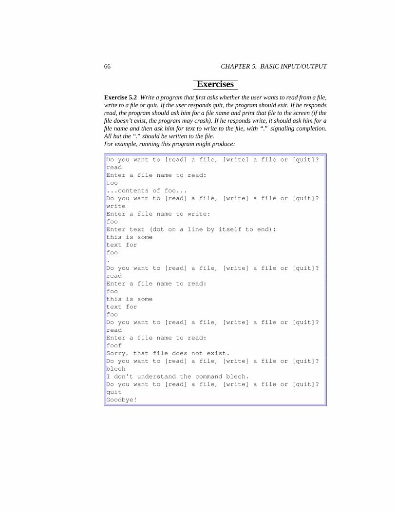
66 CHAPTER 5. BASIC INPUT/OUTPUT
ExercisesExercise 5.2 Write a program that first asks whether the user wants to read from a file,write to a file or quit. If the user responds quit, the program should exit. If he respondsread, the program should ask him for a file name and print that file to the screen (if thefile doesn’t exist, the program may crash). If he responds write, it should ask him for afile name and then ask him for text to write to the file, with “.” signaling completion.All but the “.” should be written to the file.For example, running this program might produce:
Do you want to [read] a file, [write] a file or [quit]?readEnter a file name to read:foo...contents of foo...Do you want to [read] a file, [write] a file or [quit]?writeEnter a file name to write:fooEnter text (dot on a line by itself to end):this is sometext forfoo.Do you want to [read] a file, [write] a file or [quit]?readEnter a file name to read:foothis is sometext forfooDo you want to [read] a file, [write] a file or [quit]?readEnter a file name to read:foofSorry, that file does not exist.Do you want to [read] a file, [write] a file or [quit]?blechI don’t understand the command blech.Do you want to [read] a file, [write] a file or [quit]?quitGoodbye!

Chapter 6
Modules
In Haskell, program subcomponents are divided into modules. Each module sits in itsown file and the name of the module should match the name of the file (without the“.hs” extension, of course), if you wish to ever use that module in a larger program.
For instance, suppose I am writing a game of poker. I may wish to have a separatemodule called “Cards” to handle the generation of cards, the shuffling and the dealingfunctions, and then use this “Cards” module in my “Poker” modules. That way, if Iever go back and want to write a blackjack program, I don’t have to rewrite all the codefor the cards; I can simply import the old “Cards” module.
6.1 Exports
Suppose as suggested we are writing a cards module. I have left out the implementationdetails, but suppose the skeleton of our module looks something like this:
module Cardswhere
data Card = ...data Deck = ...
newDeck :: ... -> DecknewDeck = ...
shuffle :: ... -> Deck -> Deckshuffle = ...
-- ’deal deck n’ deals ’n’ cards from ’deck’deal :: Deck -> Int -> [Card]deal deck n = dealHelper deck n []
67

68 CHAPTER 6. MODULES
dealHelper = ...
In this code, the function deal calls a helper function dealHelper. The im-plementation of this helper function is very dependent on the exact data structures youused for Card and Deck so we don’t want other people to be able to call this function.In order to do this, we create an export list, which we insert just after the module namedeclaration:
module Cards ( Card(),Deck(),newDeck,shuffle,deal
)where
...
Here, we have specified exactly what functions the module exports, so people whouse this module won’t be able to access our dealHelper function. The () afterCard and Deck specify that we are exporting the type but none of the constructors.For instance if our definition of Card were:
data Card = Card Suit Facedata Suit = Hearts
| Spades| Diamonds| Clubs
data Face = Jack| Queen| King| Ace| Number Int
Then users of our module would be able to use things of type Card, but wouldn’tbe able to construct their own Cards and wouldn’t be able to extract any of the suit/faceinformation stored in them.
If we wanted users of our module to be able to access all of this information, wewould have to specify it in the export list:
module Cards ( Card(Card),Suit(Hearts,Spades,Diamonds,Clubs),Face(Jack,Queen,King,Ace,Number),...
)

6.2. IMPORTS 69
where
...
This can get frustrating if you’re exporting datatypes with many constructors, so ifyou want to export them all, you can simply write (..), as in:
module Cards ( Card(..),Suit(..),Face(..),...
)where
...
And this will automatically export all the constructors.
6.2 Imports
There are a few idiosyncracies in the module import system, but as long as you stayaway from the corner cases, you should be fine. Suppose, as before, you wrote amodule called “Cards” which you saved in the file “Cards.hs”. You are now writingyour poker module and you want to import all the definitions from the “Cards” module.To do this, all you need to do is write:
module Pokerwhere
import Cards
This will enable to you use any of the functions, types and constructors exportedby the module “Cards”. You may refer to them simply by their name in the “Cards”module (as, for instance, newDeck), or you may refer to them explicitely as importedfrom “Cards” (as, for instance, Cards.newDeck). It may be the case that two moduleexport functions or types of the same name. In these cases, you can import one ofthe modules qualified which means that you would no longer be able to simply usethe newDeck format but must use the longer Cards.newDeck format, to removeambiguity. If you wanted to import “Cards” in this qualified form, you would write:
import qualified Cards
Another way to avoid problems with overlapping function definitions is to importonly certain functions from modules. Suppose we knew the only function from “Cards”that we wanted was newDeck, we could import only this function by writing:

70 CHAPTER 6. MODULES
import Cards (newDeck)
On the other hand, suppose we knew that that the deal function overlapped withanother module, but that we didn’t need the “Cards” version of that function. We couldhide the definition of deal and import everything else by writing:
import Cards hiding (deal)
Finally, suppose we want to import “Cards” as a qualified module, but don’t wantto have to type Cards. out all the time and would rather just type, for instance, C. –we could do this using the as keyword:
import qualified Cards as C
These options can be mixed and matched – you can give explicit import lists onqualified/as imports, for instance.
6.3 Hierarchical Imports
Though technically not part of the Haskell 98 standard, most Haskell compilers supporthierarchical imports. This was designed to get rid of clutter in the directories in whichmodules are stored. Hierarchical imports allow you to specify (to a certain degree)where in the directory structure a module exists. For instance, if you have a “haskell”directory on your computer and this directory is in your compiler’s path (see yourcompiler notes for how to set this; in GHC it’s “-i”, in Hugs it’s “-P”), then you canspecify module locations in subdirectories to that directory.
Suppose instead of saving the “Cards” module in your general haskell directory,you created a directory specifically for it called “Cards”. The full path of the Cards.hsfile is then haskell/Cards/Cards.hs (or, for Windows haskell\Cards\Cards.hs).If you then change the name of the Cards module to “Cards.Cards”, as in:
module Cards.Cards(...)where
...
You could them import it in any module, regardless of this module’s directory, as:
import Cards.Cards
If you start importing these module qualified, I highly recommend using the askeyword to shorten the names, so you can write:

6.4. LITERATE VERSUS NON-LITERATE 71
import qualified Cards.Cards as Cards
... Cards.newDeck ...
instead of:
import qualified Cards.Cards
... Cards.Cards.newDeck ...
which tends to get ugly.
6.4 Literate Versus Non-Literate
The idea of literate programming is a relatively simple one, but took quite a while tobecome popularized. When we think about programming, we think about the codebeing the default mode of entry and comments being secondary. That is, we write codewithout any special annotation, but comments are annotated with either -- or {- ...-}. Literate programming swaps these preconceptions.
There are two types of literate programs in Haskell; the first uses so-called Bird-scripts and the second uses LATEX-style markup. Each will be discussed individually.No matter which you use, literate scripts must have the extension lhs instead of hs totell the compiler that the program is written in a literate style.
6.4.1 Bird-scripts
In a Bird-style literate program, comments are default and code is introduced with aleading greater-than sign (“>”). Everything else remains the same. For example, ourHello World program would be written in Bird-style as:
This is a simple (literate!) Hello World program.
> module Main> where
All our main function does is print a string:
> main = putStrLn "Hello World"
Note that the spaces between the lines of code and the “comments” are necessary(your compiler will probably complain if you are missing them). When compiled orloaded in an interpreter, this program will have the exact same properties as the non-literate version from Section 3.4.

72 CHAPTER 6. MODULES
6.4.2 LaTeX-scripts
LATEX is a text-markup language very popular in the academic community for publish-ing. If you are unfamiliar with LATEX, you may not find this section terribly useful.
Again, a literate Hello World program written in LATEX-style would look like:
This is another simple (literate!) Hello World program.
\begin{code}module Main
where\end{code}
All our main function does is print a string:
\begin{code}main = putStrLn "Hello World"\end{code}
In LATEX-style scripts, the blank lines are not necessary.

Chapter 7
Advanced Features
Discussion
7.1 Sections and Infix Operators
We’ve already seen how to double the values of elements in a list using map:
Prelude> map (\x -> x*2) [1,2,3,4][2,4,6,8]
However, there is a more concise way to write this:
Prelude> map (*2) [1,2,3,4][2,4,6,8]
This type of thing can be done for any infix function:
Prelude> map (+5) [1,2,3,4][6,7,8,9]Prelude> map (/2) [1,2,3,4][0.5,1.0,1.5,2.0]Prelude> map (2/) [1,2,3,4][2.0,1.0,0.666667,0.5]
You might be tempted to try to subtract values from elements in a list by mapping-2 across a list. This won’t work, though, because while the + in +2 is parsed asthe standard plus operator (as there is no ambiguity), the - in -2 is interpreted as theunary minus, not the binary minus. Thus -2 here is the number −2, not the functionλx.x − 2.
In general, these are called sections. For binary infix operators (like +), we cancause the function to become prefix by enclosing it in paretheses. For example:
73

74 CHAPTER 7. ADVANCED FEATURES
Prelude> (+) 5 38Prelude> (-) 5 32
Additionally, we can provide either of its argument to make a section. For example:
Prelude> (+5) 38Prelude> (/3) 62.0Prelude> (3/) 60.5
Non-infix functions can be made infix by enclosing them in backquotes (“’’). Forexample:
Prelude> (+2) ‘map‘ [1..10][3,4,5,6,7,8,9,10,11,12]
7.2 Local Declarations
Recall back from Section 3.5, there are many computations which require using theresult of the same computation in multiple places in a function. There, we consideredthe function for computing the roots of a quadratic polynomial:
roots a b c =((-b + sqrt(b*b - 4*a*c)) / (2*a),(-b - sqrt(b*b - 4*a*c)) / (2*a))
In addition to the let bindings introduced there, we can do this using a where clause.where clauses come immediately after function definitions and introduce a new levelof layout (see Section 7.11). We write this as:
roots a b c =((-b + det) / (2*a), (-b - det) / (2*a))where det = sqrt(b*b-4*a*c)
Any values defined in a where clause shadow any other values with the same name.For instance, if we had the following code block:

7.2. LOCAL DECLARATIONS 75
det = "Hello World"
roots a b c =((-b + det) / (2*a), (-b - det) / (2*a))where det = sqrt(b*b-4*a*c)
f _ = det
The value of roots doesn’t notice the top-level declaration of det, since it isshadowed by the local definition (the fact that the types don’t match doesn’t mattereither). Furthermore, since f cannot “see inside” of roots, the only thing it knowsabout det is what is available at the top level, which is the string “Hello World.” Thus,f is a function which takes any argument to that string.
Where clauses can contain any number of subexpressions, but they must be alignedfor layout. For instance, we could also pull out the 2*a computation and get thefollowing code:
roots a b c =((-b + det) / (a2), (-b - det) / (a2))where det = sqrt(b*b-4*a*c)
a2 = 2*a
Sub-expressions in where clauses must come after function definitions. Some-times it is more convenient to put the local definitions before the actual expressionof the function. This can be done by using let/in clauses. We have already seen letclauses; where clauses are virtually identical to their let clause cousins except for theirplacement. The same roots function can be written using let as:
roots a b c =let det = sqrt (b*b - 4*a*c)
a2 = 2*ain ((-b + det) / a2, (-b - det) / a2)
Using a where clause, it looks like:
roots a b c = ((-b + det) / a2, (-b - det) / a2)wheredet = sqrt (b*b - 4*a*c)a2 = 2*a
These two types of clauses can be mixed (i.e., you can write a function which hasboth a let cause and a where clause). This is strongly advised against, as it tends tomake code difficult to read. However, if you choose to do it, values in the let clauseshadow those in the where clause. So if you define the function:

76 CHAPTER 7. ADVANCED FEATURES
f x =let y = x+1in ywhere y = x+2
The value of f 5 is 6, not 7. Of course, I plead with you to never ever writecode that looks like this. No one should have to remember this rule and by shadowingwhere-defined values in a let clause only makes your code difficult to understand.
In general, whether you should use let clauses or where clauses is largely a matterof personal preference. Usually, the names you give to the subexpressions should besufficiently expressive that without reading their definitions any reader of your codeshould be able to figure out what they do. In this case, where clauses are probablymore desirable because they allow the reader to see immediately what a function does.However, in real life, values are often given cryptic names. In which case let clausesmay be better. Either is probably okay, though I think where clauses are more common.
7.3 Partial Application
Partial application is when you take a function which takes n arguments and you supplyit with < n of them. When discussing sections in Section 7.1, we saw a form of“partial application” in which functions like + were partially applied. For instance, inthe expression map (+1) [1,2,3], the section (+1) is a partial application of +.This is because + really takes two arguments, but we’ve only given it one.
Partial application is very common in function definitions and sometimes goes bythe name “eta reduction”. For instance, suppose we are writting a function lcaseStringeta reductionwhich converts a whole string into lower case. We could write this as:
lcaseString s = map toLower s
Here, there is no partial application (though you could argue that applying no argu-ments to toLower could be considered partial application). However, we notice thatthe application of s occurs at the end of both lcaseString and of map toLower.In fact, we can remove it by performing eta reduction, to get:
lcaseString = map toLower
Now, we have a partial application of map: it expects a function and a list, butwe’ve only given it the function.
This all is related to type type of map, which is (a → b) → ([a] → [b]), whenparentheses are all included. In our case, toLower is of type Char → Char. Thus, ifwe supply this function to map, we get a function of type [Char] → [Char], as desired.
Now, consider the task of converting a string to lowercase and remove all non lettercharacters. We might write this as:

7.3. PARTIAL APPLICATION 77
lcaseLetters s = map toLower (filter isAlpha s)
But note that we can actually write this in terms of function composition:
lcaseLetters s = (map toLower . filter isAlpha) s
And again, we’re left with an eta reducible function:
lcaseLetters = map toLower . filter isAlpha
Writing functions in this style is very common among advanced Haskell users. Infact it has a name: point-free programming (not to be confused with pointless program- point-free programmingming). It is call point free because in the original definition of lcaseLetters, wecan think of the value s as a point on which the function is operating. By removing thepoint from the function definition, we have a point-free function.
A function similar to (.) is ($). Whereas (.) is function composition, ($) is $
function application. The definition of ($) from the Prelude is very simple: function application
f $ x = f x
However, this function is given very low fixity, which means that it can be used toreplace parentheses. For instance, we might write a function:
foo x y = bar y (baz (fluff (ork x)))
However, using the function application function, we can rewrite this as:
foo x y = bar y $ baz $ fluff $ ork x
This moderately resembles the function composition syntax. The ($) function isalso useful when combined with other infix functions. For instance, we cannot write:
Prelude> putStrLn "5+3=" ++ show (5+3)
because this is interpreted as (putStrLn "5+3=") ++ (show (5+3)), whichmakes no sense. However, we can fix this by writing instead:
Prelude> putStrLn $ "5+3=" ++ show (5+3)
Which works fine.Consider now the task of extracting from a list of tuples all the ones whose first
component is greater than zero. One way to write this would be:

78 CHAPTER 7. ADVANCED FEATURES
fstGt0 l = filter (\ (a,b) -> a>0) l
We can first apply eta reduction to the whole function, yielding:
fstGt0 = filter (\ (a,b) -> a>0)
Now, we can rewrite the lambda function to use the fst function instead of thepattern matching:
fstGt0 = filter (\x -> fst x > 0)
Now, we can use function composition between fst and > to get:
fstGt0 = filter (\x -> ((>0) . fst) x)
And finally we can eta reduce:
fstGt0 = filter ((>0).fst)
This definition is simultaneously shorter and easier to understand than the original.We can clearly see exactly what it is doing: we’re filtering a list by checking whethersomething is greater than zero. What are we checking? The fst element.
While converting to point free style often results in clearer code, this is of coursenot always the case. For instance, converting the following map to point free styleyields something nearly uninterpretable:
foo = map (\x -> sqrt (3+4*(xˆ2)))foo = map (sqrt . (3+) . (4*) . (ˆ2))
There are a handful of combinators defined in the Prelude which are useful for pointfree programming:
• uncurry takes a function of type a → b → c and converts it into a function oftype (a, b) → c. This is useful, for example, when mapping across a list of pairs:
Prelude> map (uncurry (*)) [(1,2),(3,4),(5,6)][2,12,30]
• curry is the opposite of uncurry and takes a function of type (a, b) → c andproduces a function of type a → b → c.
• flip reverse the order of arguments to a function. That is, it takes a function oftype a → b → c and produces a function of type b → a → c. For instance, wecan sort a list in reverse order by using flip compare:
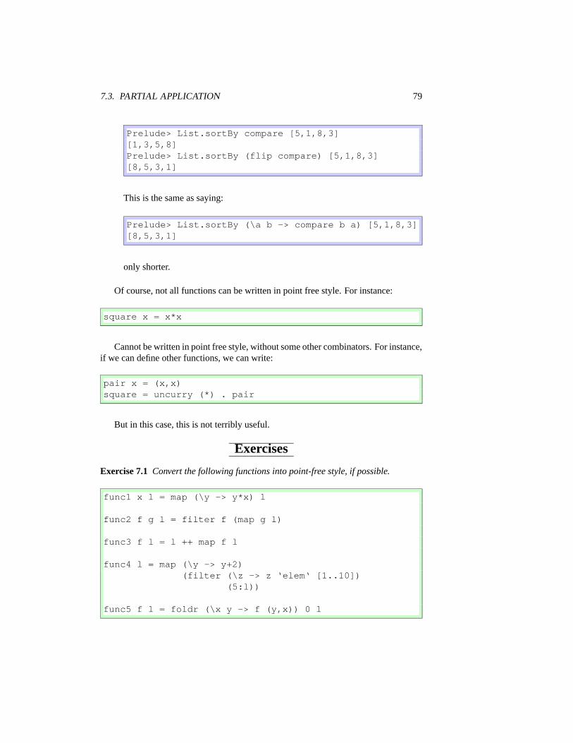
7.3. PARTIAL APPLICATION 79
Prelude> List.sortBy compare [5,1,8,3][1,3,5,8]Prelude> List.sortBy (flip compare) [5,1,8,3][8,5,3,1]
This is the same as saying:
Prelude> List.sortBy (\a b -> compare b a) [5,1,8,3][8,5,3,1]
only shorter.
Of course, not all functions can be written in point free style. For instance:
square x = x*x
Cannot be written in point free style, without some other combinators. For instance,if we can define other functions, we can write:
pair x = (x,x)square = uncurry (*) . pair
But in this case, this is not terribly useful.
Exercises
Exercise 7.1 Convert the following functions into point-free style, if possible.
func1 x l = map (\y -> y*x) l
func2 f g l = filter f (map g l)
func3 f l = l ++ map f l
func4 l = map (\y -> y+2)(filter (\z -> z ‘elem‘ [1..10])
(5:l))
func5 f l = foldr (\x y -> f (y,x)) 0 l

80 CHAPTER 7. ADVANCED FEATURES
7.4 Pattern Matching
Pattern matching is one of the most powerful features of Haskell (and most functionalprogramming languages). It is most commonly used in conjunction with case expres-sions, which we have already seen in Section 3.5. Let’s return to our Color examplefrom Section 4.5. I’ll repeat the definition we already had for the datatype:
data Color= Red| Orange| Yellow| Green| Blue| Purple| White| Black| Custom Int Int Int -- R G B componentsderiving (Show,Eq)
We then want to write a function that will convert between something of type Color
and a triple of Ints, which correspond to the RGB values, respectively. Specifically, ifwe see a Color which is Red, we want to return (255,0,0), since this is the RGBvalue for red. So we write that (remember that piecewise function definitions are justcase statements):
colorToRGB Red = (255,0,0)
If we see a Color which is Orange, we want to return (255,128,0); and if wesee Yellow, we want to return (255,255,0), and so on. Finally, if we see a customcolor, which is comprised of three components, we want to make a triple out of these,so we write:
colorToRGB Orange = (255,128,0)colorToRGB Yellow = (255,255,0)colorToRGB Green = (0,255,0)colorToRGB Blue = (0,0,255)colorToRGB Purple = (255,0,255)colorToRGB White = (255,255,255)colorToRGB Black = (0,0,0)colorToRGB (Custom r g b) = (r,g,b)
Then, in our interpreter, if we type:
Color> colorToRGB Yellow(255,255,0)

7.4. PATTERN MATCHING 81
What is happening is this: we create a value, call it x, which has value Red. Wethen apply this to colorToRGB. We check to see if we can “match” x against Red.This match fails because according to the definition of Eq Color, Red is not equalto Yellow. We continue down the definitions of colorToRGB and try to matchYellow against Orange. This fails, too. We the try to match Yellow againstYellow, which succeeds, so we use this function definition, which simply returnsthe value (255,255,0), as expected.
Suppose instead, we used a custom color:
Color> colorToRGB (Custom 50 200 100)(50,200,100)
We apply the same matching process, failing on all values from Red to Black.We then get to try to match Custom 50 200 100 against Custom r g b. Wecan see that the Custom part matches, so then we go see if the subelements match. Inthe matching, the variables r, g and b are essentially wild cards, so there is no troublematching r with 50, g with 200 and b with 100. As a “side-effect” of this matching, rgets the value 50, g gets the value 200 and b gets the value 100. So the entire matchsucceeded and we look at the definition of this part of the function and bundle up thetriple using the matched values of r, g and b.
We can also write a function to check to see if a Color is a custom color or not:
isCustomColor (Custom _ _ _) = TrueisCustomColor _ = False
When we apply a value to isCustomColor it tries to match that value againstCustom . This match will succeed if the value is Custom x y z for any x,y and z. The (underscore) character is a “wildcard” and will match anything, but willnot do the binding that would happen if you put a variable name there. If this matchsucceeds, the function returns True; however, if this match fails, it goes on to the nextline, which will match anything and then return False.
For some reason we might want to define a function which tells us whether a givencolor is “bright” or not, where my definition of “bright” is that one of its RGB compo-nents is equal to 255 (admittedly and arbitrary definition, but it’s simply an example).We could define this function as:
isBright = isBright’ . colorToRGBwhere isBright’ (255,_,_) = True
isBright’ (_,255,_) = TrueisBright’ (_,_,255) = TrueisBright’ _ = False
Let’s dwell on this definition for a second. The isBright function is the compo-sition of our previously defined function colorToRGB and a helper function isBright’,which tells us if a given RGB value is bright or not. We could replace the first line here

82 CHAPTER 7. ADVANCED FEATURES
with isBright c = isBright’ (colorToRGB c) but there is no need to ex-plicitly write the parameter here, so we don’t. Again, this function composition styleof programming takes some getting used to, so I will try to use it frequently in thistutorial.
The isBright’ helper function takes the RGB triple produced by colorToRGB.It first tries to match it against (255, , ) which succeeds if the value has 255 inits first position. If this match succeeds, isBright’ returns True and so doesisBright. The second and third line of definition check for 255 in the second andthird position in the triple, respectively. The fourth line, the fallthrough, matches ev-erything else and reports it as not bright.
We might want to also write a function to convert between RGB triples and Colors.We could simple stick everything in a Custom constructor, but this would defeat thepurpose; we want to use the Custom slot only for values which don’t match the pre-defined colors. However, we don’t want to allow the user to construct custom colorslike (600,-40,99) since these are invalid RGB values. We could throw an error if sucha value is given, but this can be difficult to deal with. Instead, we use the Maybedatatype. This is defined (in the Prelude) as:
data Maybe a = Nothing| Just a
The way we use this is as follows: our rgbToColor function returns a value oftype Maybe Color. If the RGB value passed to our function is invalid, we returnNothing, which corresponds to a failure. If, on the other hand, the RGB value isvalid, we create the appropriate Color value and return Just that. The code to do thisis:
rgbToColor 255 0 0 = Just RedrgbToColor 255 128 0 = Just OrangergbToColor 255 255 0 = Just YellowrgbToColor 0 255 0 = Just GreenrgbToColor 0 0 255 = Just BluergbToColor 255 0 255 = Just PurplergbToColor 255 255 255 = Just WhitergbToColor 0 0 0 = Just BlackrgbToColor r g b =
if 0 <= r && r <= 255 &&0 <= g && g <= 255 &&0 <= b && b <= 255
then Just (Custom r g b)else Nothing -- invalid RGB value
The first eight lines match the RGB arguments against the predefined values and,if they match, rgbToColor returns Just the appropriate color. If none of thesematches, the last definition of rgbToColor matches the first argument against r, the

7.5. GUARDS 83
second against g and the third against b (which causes the side-effect of binding thesevalues). It then checks to see if these values are valid (each is greater than or equal tozero and less than or equal to 255). If so, it returns Just (Custom r g b); if not,it returns Nothing corresponding to an invalid color.
Using this, we can write a function that checks to see if a right RGB value is valid:
rgbIsValid r g b = rgbIsValid’ (rgbToColor r g b)where rgbIsValid’ (Just _) = True
rgbIsValid’ _ = False
Here, we compose the helper function rgbIsValid’with our function rgbToColor.The helper function checks to see if the value returned by rgbToColor is Just any-thing (the wildcard). If so, it returns True. If not, it matches anything and returnsFalse.
Pattern matching isn’t magic, though. You can only match against datatypes; youcannot match against functions. For instance, the following is invalid:
f x = x + 1
g (f x) = x
Even though the intended meaning of g is clear (i.e., g x = x - 1), the com-piler doesn’t know in general that f has an inverse function, so it can’t perform matcheslike this.
7.5 Guards
Guards can be thought of as an extension to the pattern matching facility. They enableyou to allow piecewise function definitions to be taken according to arbitrary booleanexpressions. Guards appear after all arguments to a function but before the equals sign,and are begun with a vertical bar. We could use guards to write a simple function whichreturns a string telling you the result of comparing two elements:
comparison x y | x < y = "The first is less"| x > y = "The second is less"| otherwise = "They are equal"
You can read the vertical bar as “such that.” So we say that the value of comparisonx y “such that” x is less than y is “The first is less.” The value such that x is greaterthan y is “The second is less” and the value otherwise is “They are equal”. The key-word otherwise is simply defined to be equal to True and thus matches anythingthat falls through that far. So, we can see that this works:

84 CHAPTER 7. ADVANCED FEATURES
Guards> comparison 5 10"The first is less"Guards> comparison 10 5"The second is less"Guards> comparison 7 7"They are equal"
One thing to note about guards is that they are tested after pattern matching, not inconjunction with pattern matching. This means that once a pattern matches, if none ofthe guards succeed, further pattern matches will not be attempted. So, if we had insteaddefined:
comparison2 x y | x < y = "The first is less"| x > y = "The second is less"
comparison2 _ _ = "They are equal"
The intention would be that if both of the guards failed, it would “fall through” tothe final match and say that they were equal. This is not what happens, though.
Guards> comparison2 7 7*** Exception: Guards.hs:8: Non-exhaustive patterns
in function comparison2
If we think about what is happening in the compiler this makes sense. When weapply two sevens to comparison2, they are matched against x and y, which suc-ceeds and the values are bound. Pattern matching then stops completely, since it hassucceeded. The guards are then activated and x and y are compared. Neither of theguards succeeds, so an error is raised.
One nicety about guards is that where clauses are common to all guards. So anotherpossible definition for our isBright function from the previous section would be:
isBright2 c | r == 255 = True| g == 255 = True| b == 255 = True| otherwise = False
where (r,g,b) = colorToRGB c
The function is equivalent to the previous version, but performs its calculationslightly differently. It takes a color, c, and applies colorToRGB to it, yielding anRGB triple which is matched (using pattern matching!) against (r,g,b). This matchsucceeds and the values r, g and b are bound to their respective values. The first guardchecks to see if r is 255 and, if so, returns true. The second and third guard check gand b against 255, respectively and return true if they match. The last guard fires as alast resort and returns False.

7.6. INSTANCE DECLARATIONS 85
7.6 Instance Declarations
In order to declare a type to be an instance of a class, you need to provide an instancedeclaration for it. Most classes provide what’s called a “minimal complete definition.”This means the functions which must be implemented for this class in order for itsdefinition to be satisfied. Once you’ve written these functions for your type, you candeclare it an instance of the class.
7.6.1 The Eq Class
The Eq class has two members (i.e., two functions):
(==) :: Eq a => a -> a -> Bool(/=) :: Eq a => a -> a -> Bool
The first of these type signatures reads that the function == is a function which takestwo as which are members of Eq and produces a Bool. The type signature of /= (notequal) is identical. A minimal complete definition for the Eq class requires that eitherone of these functions be defined (if you define ==, then /= is defined automatically bynegating the result of ==, and vice versa). These declarations must be provided insidethe instance declaration.
This is best demonstrated by example. Suppose we have our color example, re-peded here for convenience:
data Color= Red| Orange| Yellow| Green| Blue| Purple| White| Black| Custom Int Int Int -- R G B components
We can define Color to be an instance of Eq by the following declaration:
instance Eq Color whereRed == Red = TrueOrange == Orange = TrueYellow == Yellow = TrueGreen == Green = TrueBlue == Blue = TruePurple == Purple = TrueWhite == White = True

86 CHAPTER 7. ADVANCED FEATURES
Black == Black = True(Custom r g b) == (Custom r’ g’ b’) =
r == r’ && g == g’ && b == b’_ == _ = False
The first line here begins with the keyword instance telling the compiler that we’remaking an instance declaration. It then specifies the class, Eq, and the type, Color
which is going to be an instance of this class. Following that, there’s the where key-word. Finally there’s the method declaration.
The first eight lines of the method declaration are basically identical. The first one,for instance, says that the value of the expression Red == Red is equal to True.Lines two through eight are identical. The declaration for custom colors is a bit differ-ent. We pattern match Custom on both sides of ==. On the left hand side, we bind r,g and b to the components, respectively. On the right hand side, we bind r’, g’ andb’ to the components. We then say that these two custom colors are equal preciselywhen r == r’, g == g’ and b == b’ are all equal. The fallthrough says that anypair we haven’t previously declared as equal are unequal.
7.6.2 The Show Class
The Show class is used to display arbitrary values as strings. This class has threemethods:
show :: Show a => a -> StringshowsPrec :: Show a => Int -> a -> String -> StringshowList :: Show a => [a] -> String -> String
A minimal complete definition is either show or showsPrec (we will talk aboutshowsPrec later – it’s in there for efficiency reasons). We can define our Color
datatype to be an instance of Show with the following instance declaration:
instance Show Color whereshow Red = "Red"show Orange = "Orange"show Yellow = "Yellow"show Green = "Green"show Blue = "Blue"show Purple = "Purple"show White = "White"show Black = "Black"show (Custom r g b) =
"Custom " ++ show r ++ " " ++show g ++ " " ++ show b
This declaration specifies exactly how to convert values of type Color to Strings.Again, the first eight lines are identical and simply take a Color and produce a string.

7.6. INSTANCE DECLARATIONS 87
The last line for handling custom colors matches out the RGB components and createsa string by concattenating the result of showing the components individually (withspaces in between and “Custom” at the beginning).
7.6.3 Other Important Classes
There are a few other important classes which I will mention briefly because either theyare commonly used or because we will be using them shortly. I won’t provide exampleinstance declarations; how you can do this should be clear by now.
The Ord Class
The ordering class, the functions are:
compare :: Ord a => a -> a -> Ordering(<=) :: Ord a => a -> a -> Bool(>) :: Ord a => a -> a -> Bool(>=) :: Ord a => a -> a -> Bool(<) :: Ord a => a -> a -> Boolmin :: Ord a => a -> a -> amax :: Ord a => a -> a -> a
The almost any of the functions alone is a minimal complete definition; it is rec-ommended that you implement compare if you implement only one, though. Thisfunction returns a value of type Ordering which is defined as:
data Ordering = LT | EQ | GT
So, for instance, we get:
Prelude> compare 5 7LTPrelude> compare 6 6EQPrelude> compare 7 5GT
In order to declare a type to be an instance of Ord you must already have declaredit an instance of Eq (in other words, Ord is a subclass of Eq – more about this inSection 8.4).
The Enum Class
The Enum class is for enumerated types; that is, for types where each element has asuccessor and a predecessor. It’s methods are:

88 CHAPTER 7. ADVANCED FEATURES
pred :: Enum a => a -> asucc :: Enum a => a -> atoEnum :: Enum a => Int -> afromEnum :: Enum a => a -> IntenumFrom :: Enum a => a -> [a]enumFromThen :: Enum a => a -> a -> [a]enumFromTo :: Enum a => a -> a -> [a]enumFromThenTo :: Enum a => a -> a -> a -> [a]
The minimal complete definition contains both toEnum and fromEnum, whichconverts from and to Ints. The pred and succ functions give the predecessor andsuccessor, respectively. The enum functions enumerate lists of elements. For instance,enumFrom x lists all elements after x; enumFromThen x step lists all elementsstarting at x in steps of size step. The To functions end the enumeration at the givenelement.
The Num Class
The Num class provides the standard arithmetic operations:
(-) :: Num a => a -> a -> a(*) :: Num a => a -> a -> a(+) :: Num a => a -> a -> anegate :: Num a => a -> asignum :: Num a => a -> aabs :: Num a => a -> afromInteger :: Num a => Integer -> a
All of these are obvious except for perhaps negate which is the unary minus.That is, negate x means −x.
The Read Class
The Read class is the opposite of the Show class. It is a way to take a string and readin from it a value of arbitrary type. The methods for Read are:
readsPrec :: Read a => Int -> String -> [(a, String)]readList :: String -> [([a], String)]
The minimal complete definition is readsPrec. The most important functionrelated to this is read, which uses readsPrec as:
read s = fst (head (readsPrec 0 s))

7.6. INSTANCE DECLARATIONS 89
This will fail if parsing the string fails. You could define a maybeRead functionas:
maybeRead s =case readsPrec 0 s of
[(a,_)] -> Just a_ -> Nothing
How to write and use readsPrec directly will be discussed further in the exam-ples.
7.6.4 Class Contexts
Suppose we are definition the Maybe datatype from scratch. The definition would besomething like:
data Maybe a = Nothing| Just a
Now, when we go to write the instance declarations, for, say, Eq, we need to knowthat a is an instance of Eq otherwise we can’t write a declaration. We express this as:
instance Eq a => Eq (Maybe a) whereNothing == Nothing = True(Just x) == (Just x’) == x == x’
This first line can be read “That a is an instance of Eq implies (=>) that Maybe a
is an instance of Eq.”
7.6.5 Deriving Classes
Writing obvious Eq, Ord, Read and Show classes like these is tedious and should beautomated. Luckily for us, it is. If you write a datatype that’s “simple enough” (almostany datatype you’ll write unless you start writing fixed point types), the compiler canautomatically derive some of the most basic classes. To do this, you simply add aderiving clause to after the datatype declaration, as in:
data Color= Red| ...| Custom Int Int Int -- R G B componentsderiving (Eq, Ord, Show, Read)
This will automatically create instances of the Color datatype of the named classes.Similarly, the declaration:

90 CHAPTER 7. ADVANCED FEATURES
data Maybe a = Nothing| Just aderiving (Eq, Ord, Show Read)
derives these classes just when a is appropriate.All in all, you are allowed to derive instances of Eq, Ord, Enum, Bounded,
Show and Read. There is considerable work in the area of “polytypic programming”or “generic programming” which, among other things, would allow for instance dec-larations for any class to be derived. This is much beyond the scope of this tutorial;instead, I refer you to the literature.
7.7 Datatypes Revisited
I know by this point you’re probably terribly tired of hearing about datatypes. Theyare, however, incredibly important, otherwise I wouldn’t devote so much time to them.Datatypes offer a sort of notational convenience if you have, for instance, a datatypethat holds many many values. These are called named fields.
7.7.1 Named Fields
Consider a datatype whose purpose is to hold configuration settings. Usually whenyou extract members from this type, you really only care about one or possibly two ofthe many settings. Moreover, if many of the settings have the same type, you mightoften find yourself wondering “wait, was this the fourth or fifth element?” One thingyou could do would be to write accessor functions. Consider the following made-upconfiguration type for a terminal program:
data Configuration =Configuration String -- user name
String -- local hostString -- remote hostBool -- is guest?Bool -- is super user?String -- current directoryString -- home directoryInteger -- time connected
deriving (Eq, Show)
You could then write accessor functions, like (I’ve only listed a few):
getUserName (Configuration un _ _ _ _ _ _ _) = ungetLocalHost (Configuration _ lh _ _ _ _ _ _) = lhgetRemoteHost (Configuration _ _ rh _ _ _ _ _) = rh

7.7. DATATYPES REVISITED 91
getIsGuest (Configuration _ _ _ ig _ _ _ _) = ig...
You could also write update functions to update a single element. Of course, nowif you add an element to the configuration, or remove one, all of these functions nowhave to take a different number of arguments. This is highly annoying and is an easyplace for bugs to slip in. However, there’s a solution. We simply give names to thefields in the datatype declaration, as follows:
data Configuration =Configuration { username :: String,
localhost :: String,remotehost :: String,isguest :: Bool,issuperuser :: Bool,currentdir :: String,homedir :: String,timeconnected :: Integer
}
This will automatically generate the following accessor functions for us:
username :: Configuration -> Stringlocalhost :: Configuration -> String...
Moreover, it gives us very convenient update methods. Here is a short examplefor a “post working directory” and “change directory” like functions that work onConfigurations:
changeDir :: Configuration -> String -> ConfigurationchangeDir cfg newDir =
-- make sure the directory existsif directoryExists newDir
then -- change our current directorycfg{currentdir = newDir}
else error "directory does not exist"
postWorkingDir :: Configuration -> String-- retrieve our current directory
postWorkingDir cfg = currentdir cfg
So, in general, to update the field x in a datatype y to z, you write y{x=z}. Youcan change more than one; each should be separated by commas, for instance, y{x=z,a=b, c=d}.

92 CHAPTER 7. ADVANCED FEATURES
You can of course continue to pattern match against Configurations as you didbefore. The named fields are simply syntactic sugar; you can still write something like:
getUserName (Configuration un _ _ _ _ _ _ _) = un
But there is little reason to. Finally, you can pattern match against named fields asin:
getHostData (Configuration {localhost=lh,remotehost=rh})= (lh,rh)
This matches the variable lh against the localhost field on the Configuration
and the variable rh against the remotehost field on the Configuration. Thesematches of course succeed. You could also constrain the matches by putting valuesinstead of variable names in these positions, as you would for standard datatypes.
You can create values of Configuration in the old way as shown in the first definitionbelow, or in the named-field’s type, as shown in the second definition below:
initCFG =Configuration "nobody" "nowhere" "nowhere"
False False "/" "/" 0initCFG’ =
Configuration{ username="nobody",localhost="nowhere",remotehost="nowhere",isguest=False,issuperuser=False,currentdir="/",homedir="/",timeconnected=0 }
Though the second is probably much more understandable unless you litter yourcode with comments.
7.8 More Lists
todo: put something here
7.8.1 Standard List Functions
Recall that the definition of the built-in Haskell list datatype is equivalent to:
data List a = Nil| Cons a (List a)

7.8. MORE LISTS 93
With the exception that Nil is called [] and Cons x xs is called x:xs. This issimply to make pattern matching easier and code smaller. Let’s investigate how someof the standard list functions may be written. Consider map. A definition is givenbelow:
map _ [] = []map f (x:xs) = f x : map f xs
Here, the first line says that when you map across an empty list, no matter what thefunction is, you get an empty list back. The second line says that when you map acrossa list with x as the head and xs as the tail, the result is f applied to x consed onto theresult of mapping f on xs.
The filter can be defined similarly:
filter _ [] = []filter p (x:xs) | p x = x : filter p xs
| otherwise = filter p xs
How this works should be clear. For an empty list, we return an empty list. Fora non empty list, we return the filter of the tail, perhaps with the head on the front,depending on whether it satisfies the predicate p or not.
We can define foldr as:
foldr _ z [] = zfoldr f z (x:xs) = f x (foldr f z xs)
Here, the best interpretation is that we are replacing the empty list ([]) with aparticular value and the list constructor (:) with some function. On the first line, wecan see the replacement of [] for z. Using backquotes to make f infix, we can writethe second line as:
foldr f z (x:xs) = x ‘f‘ (foldr f z xs)
From this, we can directly see how : is being replaced by f.Finally, foldl:
foldl _ z [] = zfoldl f z (x:xs) = foldl f (f z x) xs
This is slightly more complicated. Remember, z can be thought of as the currentstate. So if we’re folding across a list which is empty, we simply return the currentstate. On the other hand, if the list is not empty, it’s of the form x:xs. In this case, weget a new state by appling f to the current state z and the current list element x andthen recursively call foldl on xs with this new state.
There is another class of functions: the zip and unzip functions, which respec-tively take multiple lists and make one or take one lists and split them apart. Forinstance, zip does the following:
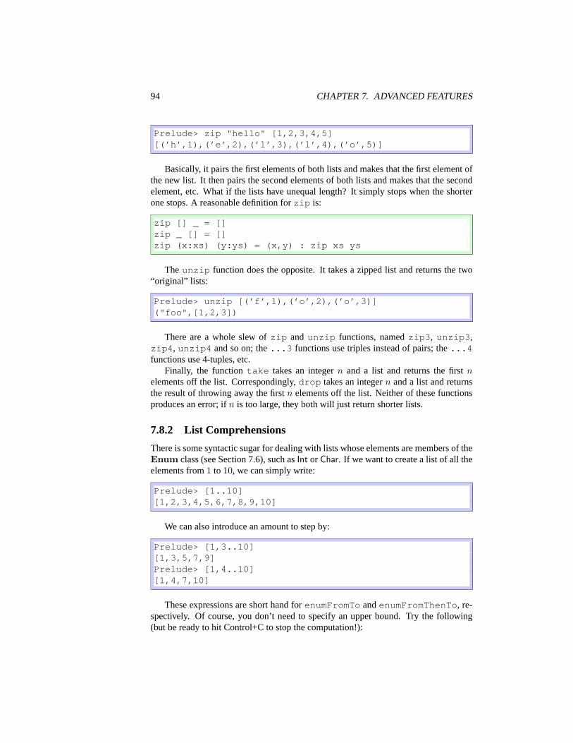
94 CHAPTER 7. ADVANCED FEATURES
Prelude> zip "hello" [1,2,3,4,5][(’h’,1),(’e’,2),(’l’,3),(’l’,4),(’o’,5)]
Basically, it pairs the first elements of both lists and makes that the first element ofthe new list. It then pairs the second elements of both lists and makes that the secondelement, etc. What if the lists have unequal length? It simply stops when the shorterone stops. A reasonable definition for zip is:
zip [] _ = []zip _ [] = []zip (x:xs) (y:ys) = (x,y) : zip xs ys
The unzip function does the opposite. It takes a zipped list and returns the two“original” lists:
Prelude> unzip [(’f’,1),(’o’,2),(’o’,3)]("foo",[1,2,3])
There are a whole slew of zip and unzip functions, named zip3, unzip3,zip4, unzip4 and so on; the ...3 functions use triples instead of pairs; the ...4functions use 4-tuples, etc.
Finally, the function take takes an integer n and a list and returns the first nelements off the list. Correspondingly, drop takes an integer n and a list and returnsthe result of throwing away the first n elements off the list. Neither of these functionsproduces an error; if n is too large, they both will just return shorter lists.
7.8.2 List Comprehensions
There is some syntactic sugar for dealing with lists whose elements are members of theEnum class (see Section 7.6), such as Int or Char. If we want to create a list of all theelements from 1 to 10, we can simply write:
Prelude> [1..10][1,2,3,4,5,6,7,8,9,10]
We can also introduce an amount to step by:
Prelude> [1,3..10][1,3,5,7,9]Prelude> [1,4..10][1,4,7,10]
These expressions are short hand for enumFromTo and enumFromThenTo, re-spectively. Of course, you don’t need to specify an upper bound. Try the following(but be ready to hit Control+C to stop the computation!):

7.8. MORE LISTS 95
Prelude> [1..][1,2,3,4,5,6,7,8,9,10,11,12{Interrupted!}
Probably yours printed a few thousand more elements than this. As we said before,Haskell is lazy. That means that a list of all numbers from 1 on is perfectly well formedand that’s exactly what this list is. Of course, if you attempt to print the list (whichwe’re implicitly doing by typing it in the interpreter), it won’t halt. But if we onlyevaluate an initial segment of this list, we’re fine:
Prelude> take 3 [1..][1,2,3]Prelude> take 3 (drop 5 [1..])[6,7,8]
This comes in useful if, say, we want to assign an ID to each element in a list.Without laziness we’d have to write something like this:
assignID :: [a] -> [(a,Int)]assignID l = zip l [1..length l]
Which means that the list will be traversed twice. However, because of laziness,we can simply write:
assignID l = zip l [1..]
And we’ll get exactly what we want. We can see that this works:
Prelude> assignID "hello"[(’h’,1),(’e’,2),(’l’,3),(’l’,4),(’o’,5)]
Finally, there is some useful syntactic sugar for map and filter, based on stan-dard set-notation in mathematics. In math, we would write something like {f(x)|x ∈s∧p(x)} to mean the set of all values of f when applied to elements of s which satisfyp. This is equivalent to the Haskell statement map f (filter p s). However, wecan also use more math-like notation and write [f x | x <- s, p x]. While inmath the ordering of the statements on the side after the pipe is free, it is not so inHaskell. We could not have put p x before x <- s otherwise the compiler wouldn’tknow yet what x was. We can use this to do simple string processing. Suppose wewant to take a string, remove all the lower-case letters and convert the rest of the lettersto upper case. We could do this in either of the following two equivalent ways:
Prelude> map toLower (filter isUpper "Hello World")"hw"Prelude> [toLower x | x <- "Hello World", isUpper x]"hw"
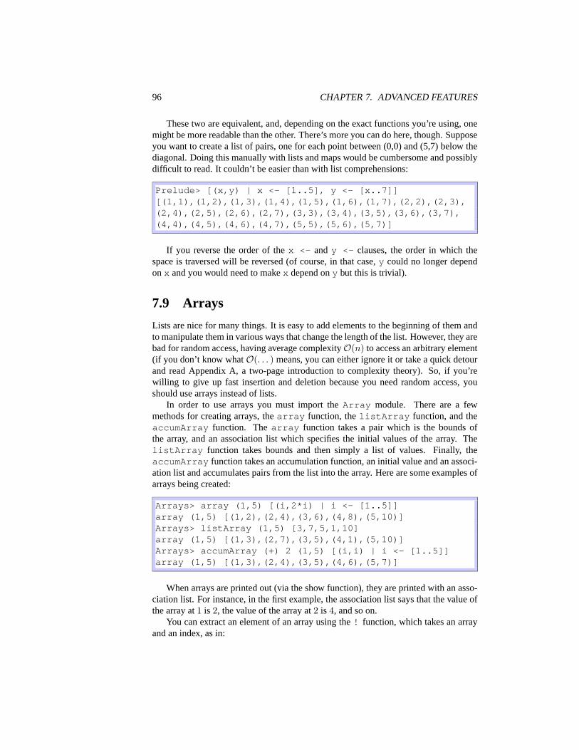
96 CHAPTER 7. ADVANCED FEATURES
These two are equivalent, and, depending on the exact functions you’re using, onemight be more readable than the other. There’s more you can do here, though. Supposeyou want to create a list of pairs, one for each point between (0,0) and (5,7) below thediagonal. Doing this manually with lists and maps would be cumbersome and possiblydifficult to read. It couldn’t be easier than with list comprehensions:
Prelude> [(x,y) | x <- [1..5], y <- [x..7]][(1,1),(1,2),(1,3),(1,4),(1,5),(1,6),(1,7),(2,2),(2,3),(2,4),(2,5),(2,6),(2,7),(3,3),(3,4),(3,5),(3,6),(3,7),(4,4),(4,5),(4,6),(4,7),(5,5),(5,6),(5,7)]
If you reverse the order of the x <- and y <- clauses, the order in which thespace is traversed will be reversed (of course, in that case, y could no longer dependon x and you would need to make x depend on y but this is trivial).
7.9 Arrays
Lists are nice for many things. It is easy to add elements to the beginning of them andto manipulate them in various ways that change the length of the list. However, they arebad for random access, having average complexity O(n) to access an arbitrary element(if you don’t know what O(. . . ) means, you can either ignore it or take a quick detourand read Appendix A, a two-page introduction to complexity theory). So, if you’rewilling to give up fast insertion and deletion because you need random access, youshould use arrays instead of lists.
In order to use arrays you must import the Array module. There are a fewmethods for creating arrays, the array function, the listArray function, and theaccumArray function. The array function takes a pair which is the bounds ofthe array, and an association list which specifies the initial values of the array. ThelistArray function takes bounds and then simply a list of values. Finally, theaccumArray function takes an accumulation function, an initial value and an associ-ation list and accumulates pairs from the list into the array. Here are some examples ofarrays being created:
Arrays> array (1,5) [(i,2*i) | i <- [1..5]]array (1,5) [(1,2),(2,4),(3,6),(4,8),(5,10)]Arrays> listArray (1,5) [3,7,5,1,10]array (1,5) [(1,3),(2,7),(3,5),(4,1),(5,10)]Arrays> accumArray (+) 2 (1,5) [(i,i) | i <- [1..5]]array (1,5) [(1,3),(2,4),(3,5),(4,6),(5,7)]
When arrays are printed out (via the show function), they are printed with an asso-ciation list. For instance, in the first example, the association list says that the value ofthe array at 1 is 2, the value of the array at 2 is 4, and so on.
You can extract an element of an array using the ! function, which takes an arrayand an index, as in:

7.10. FINITE MAPS 97
Arrays> (listArray (1,5) [3,7,5,1,10]) ! 35
Moreover, you can update elements in the array using the // function. This takesan array and an association list and updates the positions specified in the list:
Arrays> (listArray (1,5) [3,7,5,1,10]) //[(2,99),(3,-99)]
array (1,5) [(1,3),(2,99),(3,-99),(4,1),(5,10)]
There are a few other functions which are of interest:bounds returns the bounds of an arrayindices returns a list of all indices of the arrayelems returns a list of all the values in the array in orderassocs returns an association list for the array
If we define arr to be listArray (1,5) [3,7,5,1,10], the result ofthese functions applied to arr are:
Arrays> bounds arr(1,5)Arrays> indices arr[1,2,3,4,5]Arrays> elems arr[3,7,5,1,10]Arrays> assocs arr[(1,3),(2,7),(3,5),(4,1),(5,10)]
Note that while arrays are O(1) access, they are not O(1) update. They are infact O(n) update, since in order to maintain purity, the array must be copied in order tomake an update. Thus, functional arrays are pretty much only useful when you’re fillingthem up once and then only reading. If you need fast access and update, you shouldprobably use FiniteMaps, which are discussed in Section 7.10 and have O(log n)access and update.
7.10 Finite Maps
The FiniteMap datatype (which is available in the FiniteMapmodule, or Data.FiniteMapmodule in the hierarchical libraries) is a purely functional implementation of balancedtrees. Finite maps can be compared to lists are arrays in terms of the time it takes toperform various operations on those datatypes of a fixed size, n. A brief comparisonis:

98 CHAPTER 7. ADVANCED FEATURES
List Array FiniteMapinsert O(1) O(n) O(log n)update O(n) O(n) O(log n)delete O(n) O(n) O(log n)find O(n) O(1) O(log n)map O(n) O(n) O(n log n)
As we can see, lists provide fast insertion (but slow everything else), arrays pro-vide fast lookup (but slow everything else) and finite maps provide moderately fasteverything (except mapping, which is a bit slower than lists or arrays).
The type of a finite map is for the form FiniteMapkeyelt where key is the type ofthe keys and elt is the type of the elements. That is, finite maps are lookup tables fromtype key to type elt.
The basic finite map functions are:
emptyFM :: FiniteMap key eltaddToFM :: FiniteMap key elt -> key -> elt ->
FiniteMap key eltdelFromFM :: FiniteMap key elt -> key ->
FiniteMap key eltelemFM :: key -> FiniteMap key elt -> BoollookupFM :: FiniteMap key elt -> key -> Maybe elt
In all these cases, the type key must be an instance of Ord (and hence also aninstance of Eq).
There are also function listToFM and fmToList to convert lists to and fromfinite maps. Try the following:
Prelude> :m FiniteMapFiniteMap> let fm = listToFM
[(’a’,5),(’b’,10),(’c’,1),(’d’,2)]FiniteMap> let myFM = addToFM fm ’e’ 6FiniteMap> fmToList fm[(’a’,5),(’b’,10),(’c’,1),(’d’,2)]FiniteMap> fmToList myFM[(’a’,5),(’b’,10),(’c’,1),(’d’,2),(’e’,6)]FiniteMap> lookupFM myFM ’e’Just 6FiniteMap> lookupFM fm ’e’Nothing
You can also experiment with the other commands. Note that you cannot show afinite map, as they are not instances of Show:
FiniteMap> show myFM

7.11. LAYOUT 99
<interactive>:1:No instance for (Show (FiniteMap Char Integer))arising from use of ‘show’ at <interactive>:1In the definition of ‘it’: show myFM
In order to inspect the elements, you first need to use fmToList.
7.11 Layout
7.12 The Final Word on Lists
You are likely tired of hearing about lists at this point, but they are so fundamental toHaskell (and really all of functional programming) that it would be terrible not to talkabout them some more.
It turns out that foldr is actually quite a powerful function: it can compute anprimitive recursive function. A primitive recursive function is essentially one which primitive recursivecan be calculated using only “for” loops, but not “while” loops.
In fact, we can fairly easily define map in terms of foldr:
map2 f = foldr (\a b -> f a : b) []
Here, b is the accumulator (i.e., the result list) and a is the element being currentlyconsidered. In fact, we can simplify this definition through a sequence of steps:
foldr (\a b -> f a : b) []==> foldr (\a b -> (:) (f a) b) []==> foldr (\a -> (:) (f a)) []==> foldr (\a -> ((:) . f) a) []==> foldr ((:) . f) []
This is directly related to the fact that foldr (:) [] is the identity function onlists. This is because, as mentioned before, foldr f z can be thought of as replacingthe [] in lists by z and the : by f. In this case, we’re keeping both the same, so it isthe identity function.
In fact, you can convert any function of the following style into a foldr:
myfunc [] = zmyfunc (x:xs) = f x (myfunc xs)
By writing the last line with f in infix form, this should be obvious:
myfunc [] = zmyfunc (x:xs) = x ‘f‘ (myfunc xs)

100 CHAPTER 7. ADVANCED FEATURES
Clearly, we are just replacing [] with z and : with f. Consider the filterfunction:
filter p [] = []filter p (x:xs) =if p xthen x : filter p xselse filter p xs
This function also follows the form above. Based on the first line, we can figureout that z is supposed to be [], just like in the map case. Now, suppose that we callthe result of calling filter p xs simply b, then we can rewrite this as:
filter p [] = []filter p (x:xs) =if p x then x : b else b
Given this, we can transform filter into a fold:
filter p = foldr (\a b -> if p a then a:b else b) []
Let’s consider a slightly more complicated function: ++. The definition for ++ is:
(++) [] ys = ys(++) (x:xs) ys = x : (xs ++ ys)
Now, the question is whether we can write this in fold notation. First, we can applyeta reduction to the first line to give:
(++) [] = id
Through a sequence of steps, we can also eta-reduce the second line:
(++) (x:xs) ys = x : ((++) xs ys)==> (++) (x:xs) ys = (x:) ((++) xs ys)==> (++) (x:xs) ys = ((x:) . (++) xs) ys==> (++) (x:xs) = (x:) . (++) xs
Thus, we get that an eta-reduced defintion of ++ is:
(++) [] = id(++) (x:xs) = (x:) . (++) xs
Now, we can try to put this into fold notation. First, we notice that the base caseconverts [] into id. Now, if we assume (++) xs is called b and x is called a, wecan get the following definition in terms of foldr:

7.12. THE FINAL WORD ON LISTS 101
(++) = foldr (\a b -> (a:) . b) id
This actually makes sense intuitively. If we only think about applying ++ to oneargument, we can think of it as a function which takes a list and creates a functionwhich, when applied, will prepend this list to another list. In the lambda function, weassume we have a function b which will do this for the rest of the list and we need tocreate a function which will do this for b as well as the single element a. In order todo this, we first apply b and then further add a to the front.
We can further reduce this expression to a point-free style through the followingsequence:
==> (++) = foldr (\a b -> (a:) . b) id==> (++) = foldr (\a b -> (.) (a:) b) id==> (++) = foldr (\a -> (.) (a:)) id==> (++) = foldr (\a -> (.) ((:) a)) id==> (++) = foldr (\a -> ((.) . (:)) a) id==> (++) = foldr ((.) . (:)) id
This final version is point free, though not necessarily understandable. Presum-bably the original version is clearer.
As a final example, consider concat. We can write this as:
concat [] = []concat (x:xs) = x ++ concat xs
It should be immediately clear that the z element for the fold is [] and that therecursive function is ++, yielding:
concat = foldr (++) []
ExercisesExercise 7.2 The function and takes a list of booleans and returns True if and onlyif all of them are True. It also returns True on the empty list. Write this function interms of foldr.
Exercise 7.3 The function concatMap behaves such that concatMap f is the sameas concat . map f. Write this function in terms of foldr.

102 CHAPTER 7. ADVANCED FEATURES

Chapter 8
Advanced Types
As you’ve probably ascertained by this point, the type system is integral to Haskell.While this chapter is called “Advanced Types”, you will probably find it to be moregeneral than that and it must not be skipped simply because you’re not interested in thetype system.
8.1 Type Synonyms
Type synonyms exist in Haskell simply for convenience: their removal would not makeHaskell any less powerful.
Consider the case when you are constantly dealing with lists of three-dimensionalpoints. For instance, you might have a function with type [(Double,Double,Double)] → Double → [(Double,Double,Double)].Since you are a good software engineer, you want to place type signatures on all yourtop-level functions. However, typing [(Double,Double,Double)] all the time gets verytedious. To get around this, you can define a type synonym:
type List3D = [(Double,Double,Double)]
Now, the type signature for your functions may be written List3D → Double → List3D.We should note that type synonyms cannot be self-referential. That is, you cannot
have:
type BadType = Int -> BadType
This is because this is an “infinite type.” Since Haskell removes type synonymsvery early on, any instance of BadType will be replaced by Int → BadType, whichwill result in an infinite loop.
Type synonyms can also be parameterized. For instance, you might want to be ableto change the types of the points in the list of 3D points. For this, you could define:
type List3D a = [(a,a,a)]
103

104 CHAPTER 8. ADVANCED TYPES
Then your references to [(Double,Double,Double)] would become List3D Double.
8.2 Newtypes
Consider the problem in which you need to have a type which is very much like Int, butits ordering is defined differently. Perhaps you wish to order Ints first by even numbersthen by odd numbers (that is, all odd numbers are greater than any even number andwithin the odd/even subsets, ordering is standard).
Unfortunately, you cannot define a new instance of Ord for Int because thenHaskell won’t know which one to use. What you want is to define a type which isisomorphic to Int.
NOTE “Isomorphic” is a common term in mathematics which basi-cally means “structurally identical.” For instance, in graph theory, if youhave two graphs which are identical except they have different labels onthe nodes, they are isomorphic. In our context, two types are isomorphicif they have the same underlying structure.
One way to do this would be to define a new datatype:
data MyInt = MyInt Int
We could then write appropriate code for this datatype. The problem (and this isvery subtle) is that this type is not truly isomorphic to Int: it has one more value. Whenwe think of the type Int, we usually think that it takes all values of integers, but it reallyhas one more value: | (pronounced “bottom”), which is used to represent erroneous orundefined computations. Thus, MyInt has not only values MyInt 0, MyInt 1 andso on, but also MyInt | . However, since datatypes can themselves be undefined, ithas an additional value: | which differs from MyInt | and this makes the typesnon-isomorphic. (See Section ?? for more information on bottom.)
Disregarding that subtlety, there may be efficiency issues with this representation:now, instead of simply storing an integer, we have to store a pointer to an integer andhave to follow that pointer whenever we need the value of a MyInt.
To get around these problems, Haskell has a newtype construction. A newtype is across between a datatype and a type synonym: it has a constructor like a datatype, butit can have only one constructor and this constructor can have only one argument. Forinstance, we can define:
newtype MyInt = MyInt Int
But we cannot define any of:
newtype Bad1 = Bad1a Int | Bad1b Doublenewtype Bad2 = Bad2 Int Double

8.3. DATATYPES 105
Of course, the fact that we cannot define Bad2 as above is not a big issue: we cansimply define the following by pairing the types:
newtype Good2 = Good2 (Int,Double)
Now, suppose we’ve defined MyInt as a newtype. This enables use to write ourdesired instance of Ord as:
instance Ord MyInt whereMyInt i < MyInt j
| odd i && odd j = i < j| even i && even j = i < j| even i = True| otherwise = Falsewhere odd x = (x ‘mod‘ 2) == 0
even = not . odd
Like datatype, we can still derive classes like Show and Eq over newtypes (in fact,I’m implicitly assuming we have derived Eq over MyInt – where is my assumption inthe above code?).
Moreover, in recent versions of GHC (see Section 2.2), on newtypes, you are al-lowed to derive any class of which the base type (in this case, Int) is an instance. Forexample, we could derive Num on MyInt to provide arithmetic functions over it.
Pattern matching over newtypes is exactly as in datatypes. We can write constructorand destructor functions for MyInt as follows:
mkMyInt i = MyInt iunMyInt (MyInt i) = i
8.3 Datatypes
We’ve already seen datatypes used in a variety of contexts. This section concludessome of the discussion and introduces some of the common datatypes in Haskell. Italso provides a more theoretical underpinning to what datatypes actually are.
8.3.1 Strict Fields
One of the great things about Haskell is that computation is performed lazily. However,sometimes this leads to inefficiencies. One way around this problem is to use datatypeswith strict fields. Before we talk about the solution, let’s spend some time to get abit more comfortable with how bottom works in to the picture (for more theory, seeSection ??).
Suppose we’ve defined the unit datatype (this one of the simplest datatypes you candefine):
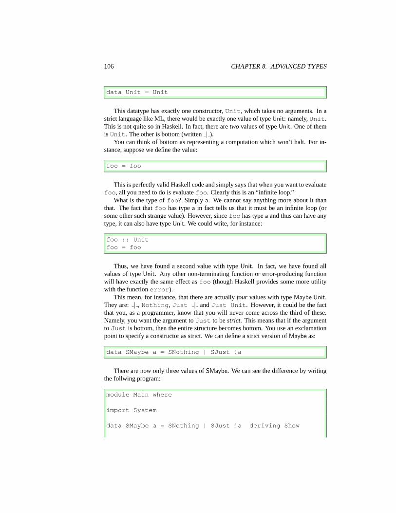
106 CHAPTER 8. ADVANCED TYPES
data Unit = Unit
This datatype has exactly one constructor, Unit, which takes no arguments. In astrict language like ML, there would be exactly one value of type Unit: namely, Unit.This is not quite so in Haskell. In fact, there are two values of type Unit. One of themis Unit. The other is bottom (written | ).
You can think of bottom as representing a computation which won’t halt. For in-stance, suppose we define the value:
foo = foo
This is perfectly valid Haskell code and simply says that when you want to evaluatefoo, all you need to do is evaluate foo. Clearly this is an “infinite loop.”
What is the type of foo? Simply a. We cannot say anything more about it thanthat. The fact that foo has type a in fact tells us that it must be an infinite loop (orsome other such strange value). However, since foo has type a and thus can have anytype, it can also have type Unit. We could write, for instance:
foo :: Unitfoo = foo
Thus, we have found a second value with type Unit. In fact, we have found allvalues of type Unit. Any other non-terminating function or error-producing functionwill have exactly the same effect as foo (though Haskell provides some more utilitywith the function error).
This mean, for instance, that there are actually four values with type Maybe Unit.They are: | , Nothing, Just | and Just Unit. However, it could be the factthat you, as a programmer, know that you will never come across the third of these.Namely, you want the argument to Just to be strict. This means that if the argumentto Just is bottom, then the entire structure becomes bottom. You use an exclamationpoint to specify a constructor as strict. We can define a strict version of Maybe as:
data SMaybe a = SNothing | SJust !a
There are now only three values of SMaybe. We can see the difference by writingthe follwing program:
module Main where
import System
data SMaybe a = SNothing | SJust !a deriving Show

8.3. DATATYPES 107
main = do[cmd] <- getArgscase cmd of"a" -> printJust undefined"b" -> printJust Nothing"c" -> printJust (Just undefined)"d" -> printJust (Just ())
"e" -> printSJust undefined"f" -> printSJust SNothing"g" -> printSJust (SJust undefined)"h" -> printSJust (SJust ())
printJust :: Maybe () -> IO ()printJust Nothing = putStrLn "Nothing"printJust (Just x) = do putStr "Just "; print x
printJust :: SMaybe () -> IO ()printSJust SNothing = putStrLn "Nothing"printSJust (SJust x) = do putStr "Just "; print x
Here, depending on what command line argument is passed, we will do somethingdifferent. The outputs for the various options are:
\% ./strict aFail: Prelude.undefined
\% ./strict bNothing
\% ./strict cJustFail: Prelude.undefined
\% ./strict dJust ()
\% ./strict eFail: Prelude.undefined
\% ./strict fNothing
\% ./strict gFail: Prelude.undefined

108 CHAPTER 8. ADVANCED TYPES
\% ./strict hJust ()
The thing worth noting here is the difference between cases “c” and “g”. In the“c” case, the Just is printed, because this is printed before the undefined value isevaluated. However, in the “g” case, since the constructor is strict, as soon as youmatch the SJust, you also match the value. In this case, the value is undefined, so thewhole thing fails before it gets a chance to do anything.
8.4 Classes
We have already encountered type classes a few times, but only in the context of pre-viously existing type classes. This section is about how to define your own. We willbegin the discussion by talking about Pong and then move on to a useful generalizationof computations.
8.4.1 Pong
The discussion here will be motivated by the construction of the game Pong (see Ap-pendix ?? for the full code). In Pong, there are three things drawn on the screen: thetwo paddles and the ball. While the paddles and the ball are different in a few respects,they share many commonalities, such as position, velocity, acceleration, color, shape,and so on. We can express these commonalities by defining a class for Pong entities,which we call Entity. We make such a definition as follows:
class Entity a wheregetPosition :: a -> (Int,Int)getVelocity :: a -> (Int,Int)getAcceleration :: a -> (Int,Int)getColor :: a -> ColorgetShape :: a -> Shape
This code defines a typeclass Entity. This class has five methods: getPosition,getVelocity, getAcceleration, getColor and getShape with the corre-sponding types.
The first line here uses the keyword class to introduce a new typeclass. We canread this typeclass definition as “There is a typeclass ’Entity’; a type ’a’ is an instanceof Entity if it provides the following five functions: . . . ”. To see how we can write aninstance of this class, let us define a player (paddle) datatype:
data Paddle =Paddle { paddlePosX, paddlePosY,
paddleVelX, paddleVelY,paddleAccX, paddleAccY :: Int,paddleColor :: Color,

8.4. CLASSES 109
paddleHeight :: Int,playerNumber :: Int }
Given this data declaration, we can define Paddle to be an instance of Entity:
instance Entity Paddle wheregetPosition p = (paddlePosX p, paddlePosY p)getVelocity p = (paddleVelX p, paddleVelY p)getAcceleration p = (paddleAccX p, paddleAccY p)getColor = paddleColorgetShape = Rectangle 5 . paddleHeight
The actual Haskell types of the class functions all have included the context Entitya =>. For example, getPosition has type Entity a ⇒ a → (Int, Int). However,it will turn out that many of our routines will need entities to also be instances of Eq.We can therefore choose to make Entity a subclass of Eq: namely, you can only bean instance of Entity if you are already an instance of Eq. To do this, we change thefirst line of the class declaration to:
class Eq a => Entity a where
Now, in order to define Paddles to be instances of Entity we will first need themto be instances of Eq – we can do this by deriving the class.
8.4.2 Computations
Let’s think back to our original motivation for defining the Maybe datatype from Sec-tion ??. We wanted to be able to express that functions (i.e., computations) can fail.
Let us consider the case of performing search on a graph. Allow us to take a smallaside to set up a small graph library:
data Graph v e = Graph [(Int,v)] [(Int,Int,e)]
The Graph datatype takes two type arguments which correspond to vertex and edgelabels. The first argument to the Graph constructor is a list (set) of vertices; the secondis the list (set) of edges. We will assume these lists are always sorted and that eachvertex has a unique id and that there is at most one edge between any two vertices.
Suppose we want to search for a path between two vertices. Perhaps there is nopath between those vertices. To represent this, we will use the Maybe datatype. Ifit succeeds, it will return the list of vertices traversed. Our search function could bewritten (naively) as follows:
search :: Graph v e -> Int -> Int -> Maybe [Int]search g@(Graph vl el) src dst
| src == dst = Just [src]
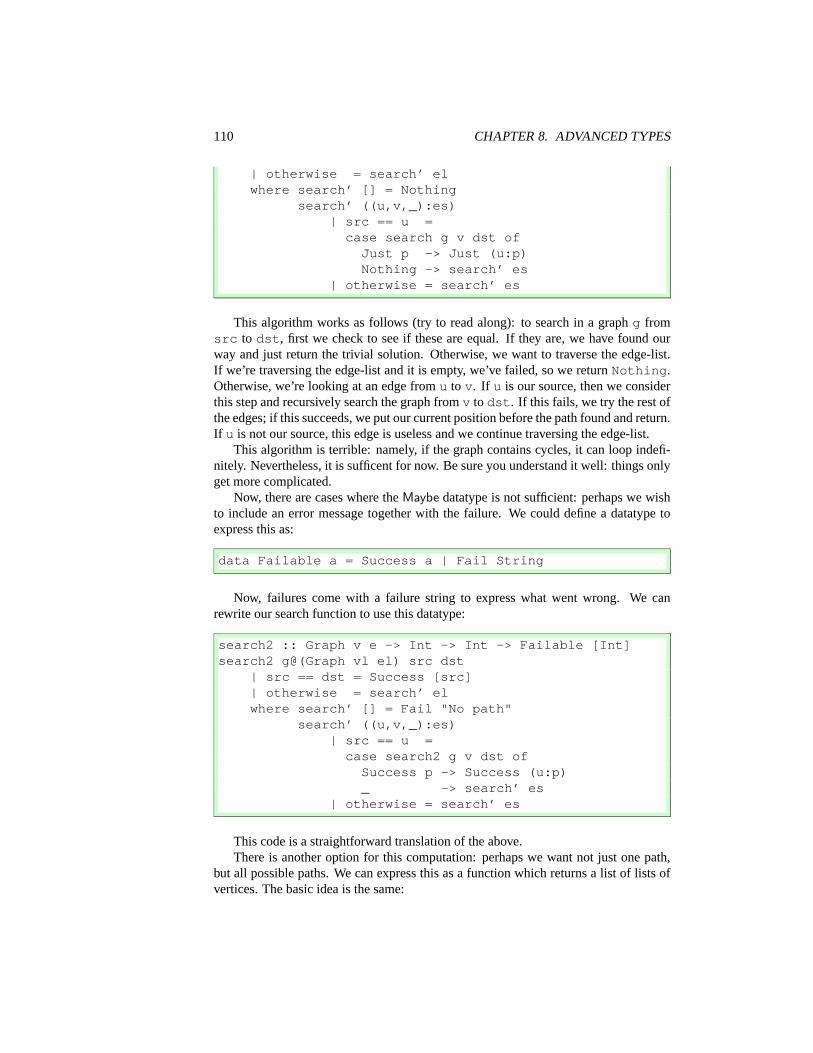
110 CHAPTER 8. ADVANCED TYPES
| otherwise = search’ elwhere search’ [] = Nothing
search’ ((u,v,_):es)| src == u =case search g v dst ofJust p -> Just (u:p)Nothing -> search’ es
| otherwise = search’ es
This algorithm works as follows (try to read along): to search in a graph g fromsrc to dst, first we check to see if these are equal. If they are, we have found ourway and just return the trivial solution. Otherwise, we want to traverse the edge-list.If we’re traversing the edge-list and it is empty, we’ve failed, so we return Nothing.Otherwise, we’re looking at an edge from u to v. If u is our source, then we considerthis step and recursively search the graph from v to dst. If this fails, we try the rest ofthe edges; if this succeeds, we put our current position before the path found and return.If u is not our source, this edge is useless and we continue traversing the edge-list.
This algorithm is terrible: namely, if the graph contains cycles, it can loop indefi-nitely. Nevertheless, it is sufficent for now. Be sure you understand it well: things onlyget more complicated.
Now, there are cases where the Maybe datatype is not sufficient: perhaps we wishto include an error message together with the failure. We could define a datatype toexpress this as:
data Failable a = Success a | Fail String
Now, failures come with a failure string to express what went wrong. We canrewrite our search function to use this datatype:
search2 :: Graph v e -> Int -> Int -> Failable [Int]search2 g@(Graph vl el) src dst
| src == dst = Success [src]| otherwise = search’ elwhere search’ [] = Fail "No path"
search’ ((u,v,_):es)| src == u =case search2 g v dst ofSuccess p -> Success (u:p)_ -> search’ es
| otherwise = search’ es
This code is a straightforward translation of the above.There is another option for this computation: perhaps we want not just one path,
but all possible paths. We can express this as a function which returns a list of lists ofvertices. The basic idea is the same:

8.4. CLASSES 111
search3 :: Graph v e -> Int -> Int -> [[Int]]search3 g@(Graph vl el) src dst
| src == dst = [[src]]| otherwise = search’ elwhere search’ [] = []
search’ ((u,v,_):es)| src == u =
map (u:) (search3 g v dst) ++search’ es
| otherwise = search’ es
The code here has gotten a little shorter, thanks to the standard prelude map func-tion, though it is essentially the same.
We may ask ourselves what all of these have in common and try to gobble upthose commonalities in a class. In essense, we need some way of representing successand some way of representing failure. Furthermore, we need a way to combine twosuccesses (in the first two cases, the first success is chosen; in the third, they are strungtogether). Finally, we need to be able to augment a previous success (if there was one)with some new value. We can fit this all into a class as follows:
class Computation c wheresuccess :: a -> c afailure :: String -> c aaugment :: c a -> (a -> c b) -> c bcombine :: c a -> c a -> c a
In this class declaration, we’re saying that c is an instance of the class Computation
if it provides four functions: success, failure, augment and combine. Thesuccess function takes a value of type a and returns it wrapped up in c, representinga successful computation. The failure function takes a String and returns a compu-tation representing a failure. The combine function takes two previous computationand produces a new one which is the combination of both. The augment function isa bit more complex.
The augment function takes some previously given computation (namely, c a)and a function which takes the value of that computation (the a) and returns a b andproduces a b inside of that computation. Note that in our current situation, givingaugment the type c a → (a → a) → c a would have been sufficient, since a is always[Int], but we make it this more general time just for generality.
How augment works is probably best shown by example. We can define Maybe,Failable and [] to be instances of Computation as:
instance Computation Maybe wheresuccess = Justfailure = const Nothing

112 CHAPTER 8. ADVANCED TYPES
augment (Just x) f = f xaugment Nothing _ = Nothingcombine Nothing y = ycombine x _ = x
Here, success is represented with Just and failure ignores its argument andreturns Nothing. The combine function takes the first success we found and ignoresthe rest. The function augment checks to see if we succeeded before (and thus hada Just something) and, if we did, applies f to it. If we failed before (and thus had aNothing), we ignore the function and return Nothing.
instance Computation Failable wheresuccess = Successfailure = Failaugment (Success x) f = f xaugment (Fail s) _ = Fail scombine (Fail _) y = ycombine x _ = x
These definitions are obvious. Finally:
instance Computation [] wheresuccess a = [a]failure = const []augment l f = concat (map f l)combine = (++)
Here, the value of a successful computation is a singleton list containing that value.Failure is represented with the empty list and to combine previous successes we simplycatentate them. Finally, augmenting a computation amounts to mapping the functionacross the list of previous computations and concatentate them. we apply the functionto each element in the list and then concatenate the results.
Using these computations, we can express all of the above versions of search as:
searchAll g@(Graph vl el) src dst| src == dst = success [src]| otherwise = search’ elwhere search’ [] = failure "no path"
search’ ((u,v,_):es)| src == u = (searchAll g v dst ‘augment‘
(success . (u:)))‘combine‘ search’ es
| otherwise = search’ es

8.5. INSTANCES 113
In this, we see the uses of all the functions from the class Computation.If you’ve understood this discussion of computations, you are in a very good posi-
tion as you have understood the concept of monads, probably the most difficult conceptin Haskell. In fact, the Computation class is almost exactly the Monad class, ex-cept that success is called return, failure is called fail and augment iscalled >>= (read “bind”). The combine function isn’t actually required by monads,but is found in the MonadPlus class for reasons which will become obvious later.
If you didn’t understand everything here, read through it again and then wait forthe proper discussion of monads in Chapter 9.
8.5 Instances
We have already seen how to declare instances of some simple classes; allow us toconsider some more advanced classes here. There is a Functor class defined in theFunctor module.
NOTE The name “functor”, like “monad” comes from category the-ory. There, a functor is like a function, but instead of mapping elementsto elements, it maps structures to structures.
The definition of the functor class is:
class Functor f wherefmap :: (a -> b) -> f a -> f b
The type definition for fmap (not to mention its name) is very similar to the func-tion map over lists. In fact, fmap is essentially a generalization of map to arbitrarystructures (and, of course, lists are already instances of Functor). However, we canalso define other structures to be instances of functors. Consider the following datatypefor binary trees:
data BinTree a = Leaf a| Branch (BinTree a) (BinTree a)
We can immediately identify that the BinTree type essentially “raises” a type a intotrees of that type. There is a naturally associated functor which goes along with thisraising. We can write the instance:
instance Functor BinTree wherefmap f (Leaf a) = Leaf (f a)fmap f (Branch left right) =
Branch (fmap f left) (fmap f right)

114 CHAPTER 8. ADVANCED TYPES
Now, we’ve seen how to make something like BinTree an instance of Eq by usingthe deriving keyword, but here we will do it by hand. We want to make BinTree asinstances of Eq but obviously we cannot do this unless a is itself an instance of Eq.We can specify this dependence in the instance declaration:
instance Eq a => Eq (BinTree a) whereLeaf a == Leaf b = a == bBranch l r == Branch l’ r’ = l == l’ && r == r’_ == _ = False
The first line of this can be read “if a is an instance of Eq, then BinTree a is alsoan instance of Eq”. We then provide the definitions. If we did not include the “Eq a=>” part, the compiler would complain because we’re trying to use the == function onas in the second line.
The “Eq a =>” part of the definition is called the “context.” We should note thatthere are some restrictions on what can appear in the context and what can appear inthe declaration. For instance, we’re not allowed to have instance declarations that don’tcontain type constructors on the right hand side. To see why, consider the followingdeclarations:
class MyEq a wheremyeq :: a -> a -> Bool
instance Eq a => MyEq a wheremyeq = (==)
As it stands, there doesn’t seem to be anything wrong with this definition. However,if elsewhere in a program we had the definition:
instance MyEq a => Eq a where(==) = myeq
In this case, if we’re trying to establish if some type is an instance of Eq, we couldreduce it to trying to find out if that type is an instance of MyEq, which we couldin turn reduce to trying to find out if that type is an instance of Eq, and so on. Thecompiler protects itself against this by refusing the first instance declaration.
This is commonly known as the closed-world assumption. That is, we’re assuming,when we write a definition like the first one, that there won’t be any declarations likethe second. However, this assumption is invalid because there’s nothing to prevent thesecond declaration (or some equally evil declaration). The closed world assumptioncan also bite you in cases like:
class OnlyInts a wherefoo :: a -> a -> Bool

8.6. KINDS 115
instance OnlyInts Int wherefoo == (==)
bar :: OnlyInts a => a -> Boolbar = foo 5
We’ve again made the closed-world assumption: we’ve assumed that the only in-stance of OnlyInts is Int, but there’s no reason another instance couldn’t be definedelsewhere, ruining our defintion of bar.
8.6 Kinds
Let us take a moment and think about what types are available in Haskell. We havesimple types, like Int, Char, Double and so on. We then have type constructors likeMaybe which take a type (like Char) and produce a new type, Maybe Char. Similarly,the type constructor [] (lists) takes a type (like Int) and produces [Int]. We have morecomplex things like → (function arrow) which takes two types (say Int and Bool) andproduces a new type Int → Bool.
In a sense, these types themselves have type. Types like Int have some sort of basictype. Types like Maybe have a type which takes something of basic type and returnssomething of basic type. And so forth.
Talking about the types of types becomes unwieldy and highly ambiguous, so wecall the types of types “kinds.” What we have been calling “basic types” have kind“*”. Something of kind * is something which can have an actual value. There is also asingle kind constructor, → with which we can build more complex kinds.
Consider Maybe. This takes something of kind * and produces something of kind*. Thus, the kind of Maybe is * -> *. Recall the definition of Pair from Sec-tion 4.5.1:
data Pair a b = Pair a b
Here, Pair is a type constructor which takes two arguments, each of kind * andproduces a type of kind *. Thus, the kind of Pair is * -> (* -> *). However, weagain assume associativity so we just write * -> * -> *.
Let us make a slightly strange datatype definition:
data Strange c a b =MkStrange (c a) (c b)
Before we analyze the kind of Strange, let’s think about what it does. It is essen-tially a pairing constructor, though it doesn’t pair actual elements, but elements withinanother constructor. For instance, think of c as Maybe. Then MkStrange pairs Maybesof the two types a and b. However, c need not be Maybe but could instead by [], ormany other things.

116 CHAPTER 8. ADVANCED TYPES
What do we know about c, though? We know that it must have kind * -> *. Thisis because we have c a on the right hand side. The type variables a and b each havekind * as before. Thus, the kind of Strange is (* -> *) -> * -> * -> *. Thatis, it takes a constructor (c) of kind * -> * together with two types of kind * andproduces something of kind *.
A question may arise regarding how we know a has kind * and not some otherkind k. In fact, the inferred kind for Strange is (k -> *) -> k -> k -> *.However, this requires polymorphism on the kind level, which is too complex, so wemake a default assumption that k = *.
NOTE There are extensions to GHC which allow you to specify thekind of constructors directly. For instance, if you wanted a different kind,you could write this explicitly:
data Strange (c :: (* -> *) -> *) a b = MkStrange (c a) (c b)
to give a different kind to Strange.
The notation of kinds suggests that we can perform partial application, as we canfor functions. And, in fact, we can. For instance, we could have:
type MaybePair = Strange Maybe
The kind of MaybePair is, not surprisingly, * -> * -> *.We should note here that all of the following definitions are acceptable:
type MaybePair1 = Strange Maybetype MaybePair2 a = Strange Maybe atype MaybePair3 a b = Strange Maybe a b
These all appear to be the same, but they are in fact not identical as far as Haskell’stype system is concerned. The following are all valid type definitions using the above:
type MaybePair1a = MaybePair1type MaybePair1b = MaybePair1 Inttype MaybePair1c = MaybePair1 Int Double
type MaybePair2b = MaybePair2 Inttype MaybePair2c = MaybePair2 Int Double
type MaybePair3c = MaybePair3 Int Double
But the following are not valid:

8.7. CLASS HIERARCHIES 117
type MaybePair2a = MaybePair2
type MaybePair3a = MaybePair3type MaybePair3b = MaybePair3 Int
This is because while it is possible to partially apply type constructors on datatypes,it is not possible on type synonyms. For instance, the reason MaybePair2a is invalidis because MaybePair2 is defined as a type synonym with one argument and we havegiven it none. The same applies for the invalid MaybePair3 definitions.
8.7 Class Hierarchies
8.8 Default
what is it?

118 CHAPTER 8. ADVANCED TYPES

Chapter 9
Monads
The most difficult concept to master, while learning Haskell, is that of understandingand using monads. We can distinguish two subcomponents here: (1) learning howto use existing monads and (2) learning how to write new ones. If you want to useHaskell, you must learn to use existing monads. On the other hand, you will only needto learn to write your own monads if you want to become a “super Haskell guru.” Still,if you can grasp writing your own monads, programming in Haskell will be much morepleasant.
So far we’ve seen two uses of monads. The first use was IO actions: We’ve seenthat, by using monads, we can abstract get away from the problems plaguing the Real-World solution to IO presented in Chapter 5. The second use was representing differenttypes of computations in Section 8.4.2. In both cases, we needed a way to sequenceoperations and saw that a sufficient definition (at least for computations) was: computations
class Computation c wheresuccess :: a -> c afailure :: String -> c aaugment :: c a -> (a -> c b) -> c bcombine :: c a -> c a -> c a
Let’s see if this definition will enable us to also perform IO. Essentially, we needa way to represent taking a value out of an action and performing some new operationon it (as in the example from Section 4.4.3, rephrased slightly):
main = dos <- readFile "somefile"putStrLn (show (f s))
But this is exactly what augment does. Using augment, we can write the abovecode as:
119

120 CHAPTER 9. MONADS
main = -- note the lack of a "do"readFile "somefile" ‘augment‘ \s ->putStrLn (show (f s))
This certainly seems to be sufficient. And, in fact, it turns out to be more thansufficient.
The definition of a monad is a slightly trimmed-down version of our Computation
class. The Monad class has four methods (but the fourth method can be defined interms of the third):
class Monad m wherereturn :: a -> m afail :: String -> m a(>>=) :: m a -> (a -> m b) -> m b(>>) :: m a -> m b -> m b
In this definition, return is equivalent to our success; fail is equivalent toour failure; and >>= (read: “bind” ) is equivalent to our augment. The >> (read:bind“then” ) method is simply a version of >>= that ignores the a. This will turn out to bethenuseful; although, as mentioned before, it can be defined in terms of >>=:
a >> x = a >>= \_ -> x
9.1 Do Notation
We have hinted that there is a connection between monads and the do notation. Here,we make that relationship concrete. There is actually nothing magic about the donotation – it is simply “syntactic sugar” for monadic operations.syntactic sugar
As we mentioned earlier, using our Computation class, we could define ourabove program as:
main =readFile "somefile" ‘augment‘ \s ->putStrLn (show (f s))
But we now know that augment is called >>= in the monadic world. Thus, thisprogram really reads:
main =readFile "somefile" >>= \s ->putStrLn (show (f s))

9.1. DO NOTATION 121
And this is completely valid Haskell at this point: if you defined a function f ::Show a => String -> a, you could compile and run this program)
This suggests that we can translate:
x <- fg x
into f >>= \x -> g x. This is exactly what the compiler does. Talking aboutdo becomes easier if we do not use implicit layout (see Section ?? for how to do this).There are four translation rules:
1. do {e} → e
2. do {e; es} → e >> do {es}
3. do {let decls; es} → let decls in do {es}
4. do {p <- e; es}→ let ok p = do {es} ; ok = fail "..."in e >>= ok
Again, we will elaborate on these one at a time:
Translation Rule 1
The first translation rule, do {e} → e, states (as we have stated before) that whenperforming a single action, having a do or not is irrelevant. This is essentially the basecase for an inductive definition of do. The base case has one action (namely e here);the other three translation rules handle the cases where there is more than one action.
Translation Rule 2
This states that do {e; es} → e >> do {es}. This tells us what to do if we havean action (e) followed by a list of actions (es). Here, we make use of the >> function,defined earlier. This rule simple states that to do {e; es}, we first perform the actione, throw away the result, and then do es.
For instance, if e is putStrLn s for some string s, then the translation of do{e; es} is to perform e (i.e., print the string) and then do es. This is clearly whatwe want.
Translation Rule 3
This states that do {let decls; es} → let decls in do {es}. This ruletells us how to deal with lets inside of a do statement. We lift the declarations within letthe let out and do whatever comes after the declarations.

122 CHAPTER 9. MONADS
Translation Rule 4
This states that do {p <- e; es}→ let ok p = do {es} ; ok = fail"..." in e >>= ok. Again, it is not exactly obvious what is going on here. How-ever, an alternate formulation of this rule, which is roughly equivalent, is: do {p <-e; es} → e >>= \p -> es. Here, it is clear what is happening. We run theaction e, and then send the results into es, but first give the result the name p.
The reason for the complex definition is that p doesn’t need to simply be a variable;it could be some complex pattern. For instance, the following is valid code:
foo = do (’a’:’b’:’c’:x:xs) <- getLineputStrLn (x:xs)
In this, we’re assuming that the results of the action getLine will begin withthe string “abc” and will have at least one more character. The question becomeswhat should happen if this pattern match fails. The compiler could simply throw anerror, like usual, for failed pattern matches. However, since we’re within a monad, wehave access to a special fail function, and we’d prefer to fail using that function,rather than the “catch all” error function. Thus, the translation, as defined, allowsthe compiler to fill in the ... with an appropriate error message about the patternmatching having failed. Apart from this, the two definitions are equivalent.
9.2 Definition
There are three rules that all monads must obey called the “Monad Laws” (and it is upmonad lawsto you to ensure that your monads obey these rules) :
1. return a >>= f ≡ f a
2. f >>= return ≡ f
3. f >>= (\x -> g x >>= h) ≡ (f >>= g) >>= h
Let’s look at each of these individually:
Law 1
This states that return a >>= f ≡ f a. Suppose we think about monads as com-putations. This means that if we create a trivial computation that simply returns thevalue a regardless of anything else (this is the return a part); and then bind it to-gether with some other computation f, then this is equivalent to simply performing thecomputation f on a directly.
For example, suppose f is the function putStrLn and a is the string “HelloWorld.” This rule states that binding a computation whose result is “Hello World”to putStrLn is the same as simply printing it to the screen. This seems to makesense.
In do notation, this law states that the following two programs are equivalent:
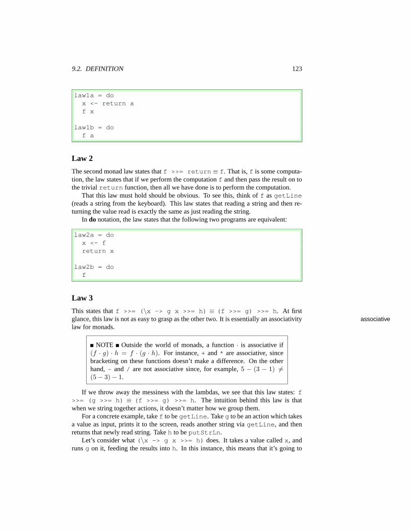
9.2. DEFINITION 123
law1a = dox <- return af x
law1b = dof a
Law 2
The second monad law states that f >>= return ≡ f. That is, f is some computa-tion, the law states that if we perform the computation f and then pass the result on tothe trivial return function, then all we have done is to perform the computation.
That this law must hold should be obvious. To see this, think of f as getLine(reads a string from the keyboard). This law states that reading a string and then re-turning the value read is exactly the same as just reading the string.
In do notation, the law states that the following two programs are equivalent:
law2a = dox <- freturn x
law2b = dof
Law 3
This states that f >>= (\x -> g x >>= h) ≡ (f >>= g) >>= h. At firstglance, this law is not as easy to grasp as the other two. It is essentially an associativity associativelaw for monads.
NOTE Outside the world of monads, a function · is associative if(f · g) · h = f · (g · h). For instance, + and * are associative, sincebracketing on these functions doesn’t make a difference. On the otherhand, - and / are not associative since, for example, 5 − (3 − 1) 6=(5 − 3) − 1.
If we throw away the messiness with the lambdas, we see that this law states: f>>= (g >>= h) ≡ (f >>= g) >>= h. The intuition behind this law is thatwhen we string together actions, it doesn’t matter how we group them.
For a concrete example, take f to be getLine. Take g to be an action which takesa value as input, prints it to the screen, reads another string via getLine, and thenreturns that newly read string. Take h to be putStrLn.
Let’s consider what (\x -> g x >>= h) does. It takes a value called x, andruns g on it, feeding the results into h. In this instance, this means that it’s going to

124 CHAPTER 9. MONADS
take a value, print it, read another value and then print that. Thus, the entire left handside of the law first reads a string and then does what we’ve just described.
On the other hand, consider (f >>= g). This action reads a string from thekeyboard, prints it, and then reads another string, returning that newly read string as aresult. When we bind this with h as on the right hand side of the law, we get an actionthat does the action described by (f >>= g), and then prints the results.
Clearly, these two actions are the same.While this explanation is quite complicated, and the text of the law is also quite
complicated, the actual meaning is simple: if we have three actions, and we composethem in the same order, it doesn’t matter where we put the parentheses. The rest is justnotation.
In do notation, says that the following two programs are equivalent:
law3a = dox <- fdo g <- x
h y
law3b = doy <- do x <- f
g xh y
9.3 A Simple State Monad
One of the simplest monads that we can craft is a state-passing monad. In Haskell, allstate information usually must be passed to functions explicitly as arguments. Usingmonads, we can effectively hide some state information.
Suppose we have a function f of type a → b, and we need to add state to thisfunction. In general, if state is of type state, we can encode it by changing the type off to a → state → (state, b). That is, the new version of f takes the original parameterof type a and a new state parameter. And, in addition to returning the value of type b,it also returns an updated state, encoded in a tuple.
For instance, suppose we have a binary tree defined as:
data Tree a= Leaf a| Branch (Tree a) (Tree a)
Now, we can write a simple map function to apply some function to each value inthe leaves:
mapTree :: (a -> b) -> Tree a -> Tree bmapTree f (Leaf a) = Leaf (f a)
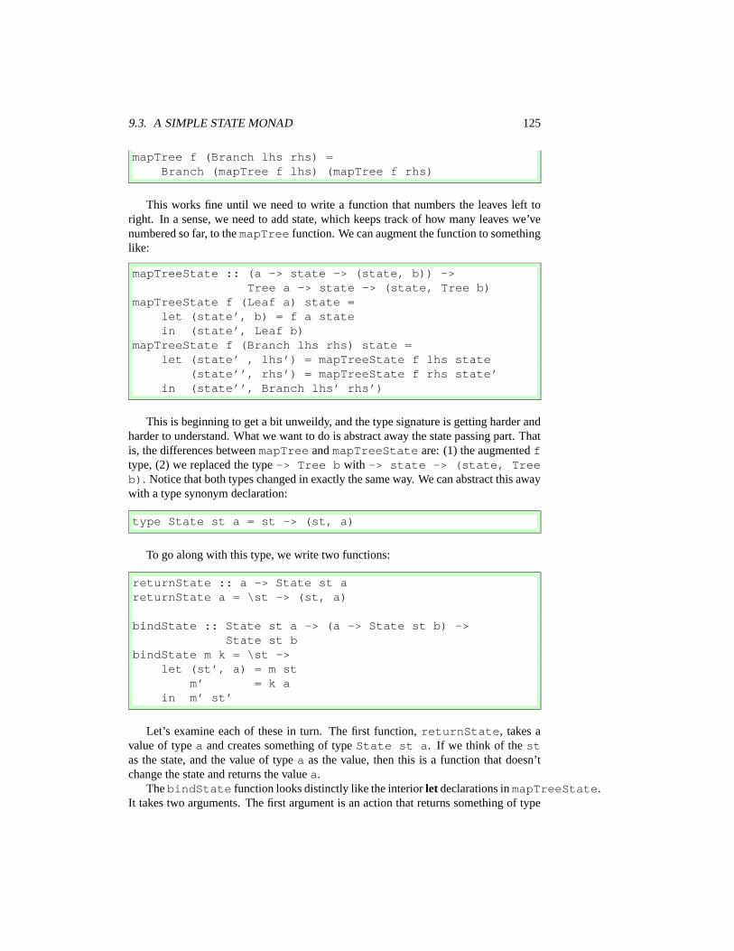
9.3. A SIMPLE STATE MONAD 125
mapTree f (Branch lhs rhs) =Branch (mapTree f lhs) (mapTree f rhs)
This works fine until we need to write a function that numbers the leaves left toright. In a sense, we need to add state, which keeps track of how many leaves we’venumbered so far, to the mapTree function. We can augment the function to somethinglike:
mapTreeState :: (a -> state -> (state, b)) ->Tree a -> state -> (state, Tree b)
mapTreeState f (Leaf a) state =let (state’, b) = f a statein (state’, Leaf b)
mapTreeState f (Branch lhs rhs) state =let (state’ , lhs’) = mapTreeState f lhs state
(state’’, rhs’) = mapTreeState f rhs state’in (state’’, Branch lhs’ rhs’)
This is beginning to get a bit unweildy, and the type signature is getting harder andharder to understand. What we want to do is abstract away the state passing part. Thatis, the differences between mapTree and mapTreeState are: (1) the augmented ftype, (2) we replaced the type -> Tree b with -> state -> (state, Treeb). Notice that both types changed in exactly the same way. We can abstract this awaywith a type synonym declaration:
type State st a = st -> (st, a)
To go along with this type, we write two functions:
returnState :: a -> State st areturnState a = \st -> (st, a)
bindState :: State st a -> (a -> State st b) ->State st b
bindState m k = \st ->let (st’, a) = m st
m’ = k ain m’ st’
Let’s examine each of these in turn. The first function, returnState, takes avalue of type a and creates something of type State st a. If we think of the stas the state, and the value of type a as the value, then this is a function that doesn’tchange the state and returns the value a.
The bindState function looks distinctly like the interior let declarations in mapTreeState.It takes two arguments. The first argument is an action that returns something of type
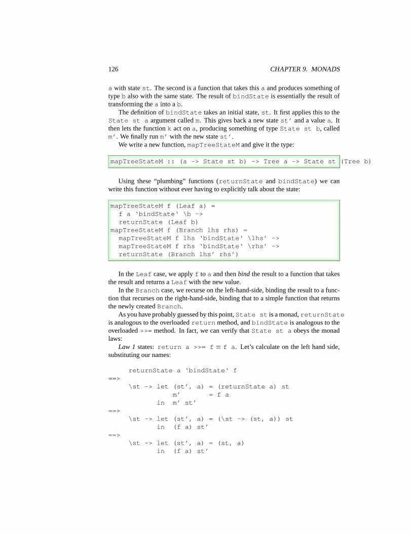
126 CHAPTER 9. MONADS
a with state st. The second is a function that takes this a and produces something oftype b also with the same state. The result of bindState is essentially the result oftransforming the a into a b.
The definition of bindState takes an initial state, st. It first applies this to theState st a argument called m. This gives back a new state st’ and a value a. Itthen lets the function k act on a, producing something of type State st b, calledm’. We finally run m’ with the new state st’.
We write a new function, mapTreeStateM and give it the type:
mapTreeStateM :: (a -> State st b) -> Tree a -> State st (Tree b)
Using these “plumbing” functions (returnState and bindState) we canwrite this function without ever having to explicitly talk about the state:
mapTreeStateM f (Leaf a) =f a ‘bindState‘ \b ->returnState (Leaf b)
mapTreeStateM f (Branch lhs rhs) =mapTreeStateM f lhs ‘bindState‘ \lhs’ ->mapTreeStateM f rhs ‘bindState‘ \rhs’ ->returnState (Branch lhs’ rhs’)
In the Leaf case, we apply f to a and then bind the result to a function that takesthe result and returns a Leaf with the new value.
In the Branch case, we recurse on the left-hand-side, binding the result to a func-tion that recurses on the right-hand-side, binding that to a simple function that returnsthe newly created Branch.
As you have probably guessed by this point, State st is a monad, returnStateis analogous to the overloaded return method, and bindState is analogous to theoverloaded >>= method. In fact, we can verify that State st a obeys the monadlaws:
Law 1 states: return a >>= f ≡ f a. Let’s calculate on the left hand side,substituting our names:
returnState a ‘bindState‘ f==>
\st -> let (st’, a) = (returnState a) stm’ = f a
in m’ st’==>
\st -> let (st’, a) = (\st -> (st, a)) stin (f a) st’
==>\st -> let (st’, a) = (st, a)
in (f a) st’

9.3. A SIMPLE STATE MONAD 127
==>\st -> (f a) st
==>f a
In the first step, we simply substitute the definition of bindState. In the secondstep, we simplify the last two lines and substitute the definition of returnState. Inthe third step, we apply st to the lambda function. In the fourth step, we rename st’to st and remove the let. In the last step, we eta reduce.
Moving on to Law 2, we need to show that f >>= return ≡ f. This is shownas follows:
f ‘bindState‘ returnState==>
\st -> let (st’, a) = f stin (returnState a) st’
==>\st -> let (st’, a) = f st
in (\st -> (st, a)) st’==>
\st -> let (st’, a) = f stin (st’, a)
==>\st -> f st
==>f
Finally, we need to show that State obeys the third law: f >>= (\x -> g x>>= h) ≡ (f >>= g) >>= h. This is much more involved to show, so we willonly sketch the proof here. Notice that we can write the left-hand-side as:
\st -> let (st’, a) = f stin (\x -> g x ‘bindState‘ h) a st’
==>\st -> let (st’, a) = f st
in (g a ‘bindState‘ h) st’==>
\st -> let (st’, a) = f stin (\st’ -> let (st’’, b) = g a
in h b st’’) st’==>
\st -> let (st’ , a) = f st(st’’, b) = g a st’(st’’’,c) = h b st’’
in (st’’’,c)

128 CHAPTER 9. MONADS
The interesting thing to note here is that we have both action applications on thesame let level. Since let is associative, this means that we can put whichever bracketingwe prefer and the results will not change. Of course, this is an informal, “hand waving”argument and it would take us a few more derivations to actually prove, but this givesthe general idea.
Now that we know that State st is actually a monad, we’d like to make it aninstance of the Monad class. Unfortunately, the straightforward way of doing thisdoesn’t work. We can’t write:
instance Monad (State st) where { ... }
This is because you cannot make instances out of non-fully-applied type synonyms.Instead, what we need to do instead is convert the type synonym into a newtype, as:
newtype State st a = State (st -> (st, a))
Unfortunately, this means that we need to do some packing and unpacking of theState constructor in the Monad instance declaration, but it’s not terribly difficult:
instance Monad (State state) wherereturn a = State (\state -> (state, a))State run >>= action = State run’
where run’ st =let (st’, a) = run st
State run’’ = action ain run’’ st’
Now, we can write our mapTreeM function as:mapTreeM
mapTreeM :: (a -> State state b) -> Tree a ->State state (Tree b)
mapTreeM f (Leaf a) = dob <- f areturn (Leaf b)
mapTreeM f (Branch lhs rhs) = dolhs’ <- mapTreeM f lhsrhs’ <- mapTreeM f rhsreturn (Branch lhs’ rhs’)
which is significantly cleaner than before. In fact, if we remove the type signature, weget the more general type:
mapTreeM :: Monad m => (a -> m b) -> Tree a ->m (Tree b)

9.3. A SIMPLE STATE MONAD 129
That is, mapTreeM can be run in any monad, not just our State monad.Now, the nice thing about encapsulating the stateful aspect of the computation like
this is that we can provide functions to get and change the current state. These looklike: getState
putStategetState :: State state stategetState = State (\state -> (state, state))
putState :: state -> State state ()putState new = State (\_ -> (new, ()))
Here, getState is a monadic operation that takes the current state, passes itthrough unchanged, and then returns it as the value. The putState function takes anew state and produces an action that ignores the current state and inserts the new one.
Now, we can write our numberTree function as:
numberTree :: Tree a -> State Int (Tree (a, Int))numberTree tree = mapTreeM number tree
where number v = docur <- getStateputState (cur+1)return (v,cur)
Finally, we need to be able to run the action by providing an initial state:
runStateM :: State state a -> state -> arunStateM (State f) st = snd (f st)
Now, we can provide an example Tree:
testTree =Branch(Branch
(Leaf ’a’)(Branch(Leaf ’b’)(Leaf ’c’)))
(Branch(Leaf ’d’)(Leaf ’e’))
and number it:
State> runStateM (numberTree testTree) 1Branch (Branch (Leaf (’a’,1)) (Branch (Leaf (’b’,2))
(Leaf (’c’,3)))) (Branch (Leaf (’d’,4))(Leaf (’e’,5)))

130 CHAPTER 9. MONADS
This may seem like a large amount of work to do something simple. However,note the new power of mapTreeM. We can also print out the leaves of the tree in aleft-to-right fashion as:
State> mapTreeM print testTree’a’’b’’c’’d’’e’
This crucially relies on the fact that mapTreeM has the more general type involvingarbitrary monads – not just the state monad. Furthermore, we can write an action thatwill make each leaf value equal to its old value as well as all the values preceeding:
fluffLeaves tree = mapTreeM fluff treewhere fluff v = do
cur <- getStateputState (v:cur)return (v:cur)
and can see it in action:
State> runStateM (fluffLeaves testTree) []Branch (Branch (Leaf "a") (Branch (Leaf "ba")
(Leaf "cba"))) (Branch (Leaf "dcba")(Leaf "edcba"))
In fact, you don’t even need to write your own monad instance and datatype. Allthis is built in to the Control.Monad.State module. There, our runStateMis called evalState; our getState is called get; and our putState is calledput.
This module also contains a state transformer monad, which we will discuss inSection 9.7.
9.4 Common Monads
It turns out that many of our favorite datatypes are actually monads themselves. Con-sider, for instance, lists. They have a monad definition that looks something like:lists
instance Monad [] wherereturn x = [x]l >>= f = concatMap f lfail _ = []
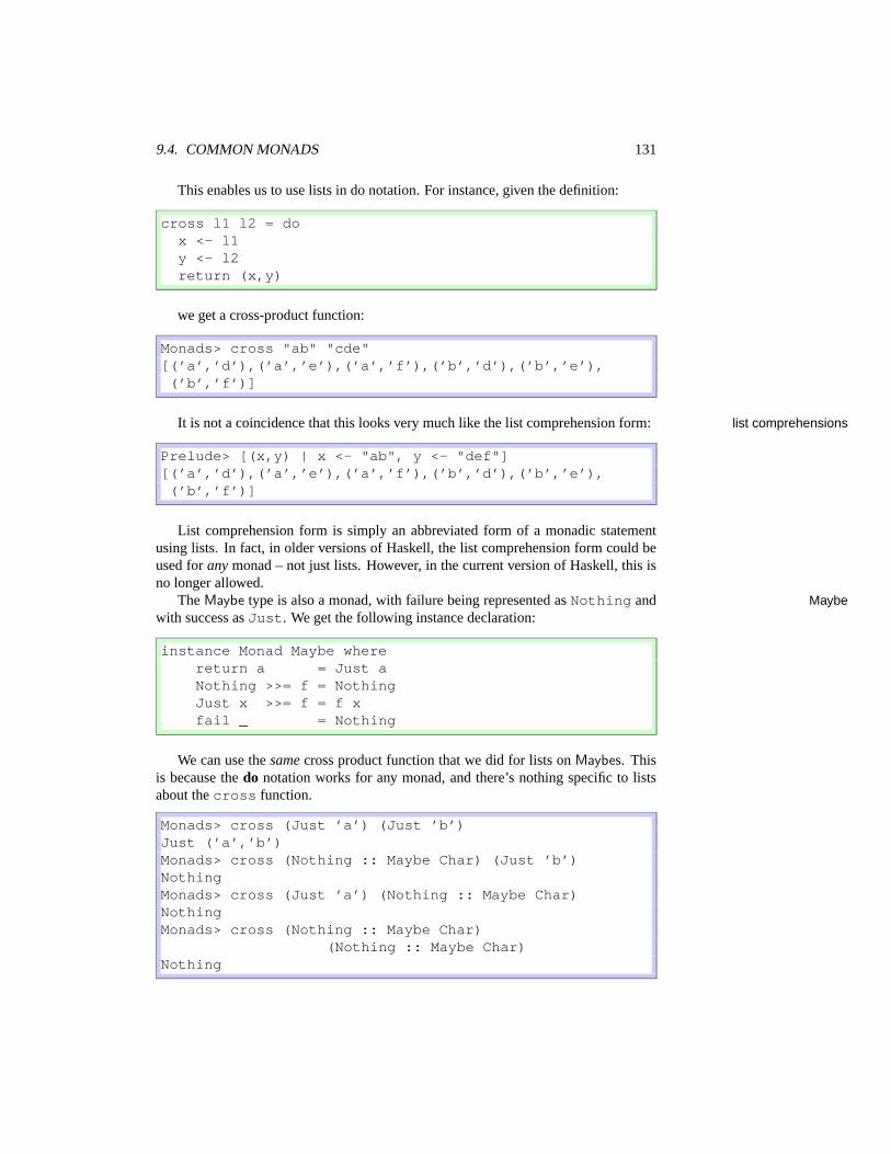
9.4. COMMON MONADS 131
This enables us to use lists in do notation. For instance, given the definition:
cross l1 l2 = dox <- l1y <- l2return (x,y)
we get a cross-product function:
Monads> cross "ab" "cde"[(’a’,’d’),(’a’,’e’),(’a’,’f’),(’b’,’d’),(’b’,’e’),(’b’,’f’)]
It is not a coincidence that this looks very much like the list comprehension form: list comprehensions
Prelude> [(x,y) | x <- "ab", y <- "def"][(’a’,’d’),(’a’,’e’),(’a’,’f’),(’b’,’d’),(’b’,’e’),(’b’,’f’)]
List comprehension form is simply an abbreviated form of a monadic statementusing lists. In fact, in older versions of Haskell, the list comprehension form could beused for any monad – not just lists. However, in the current version of Haskell, this isno longer allowed.
The Maybe type is also a monad, with failure being represented as Nothing and Maybewith success as Just. We get the following instance declaration:
instance Monad Maybe wherereturn a = Just aNothing >>= f = NothingJust x >>= f = f xfail _ = Nothing
We can use the same cross product function that we did for lists on Maybes. Thisis because the do notation works for any monad, and there’s nothing specific to listsabout the cross function.
Monads> cross (Just ’a’) (Just ’b’)Just (’a’,’b’)Monads> cross (Nothing :: Maybe Char) (Just ’b’)NothingMonads> cross (Just ’a’) (Nothing :: Maybe Char)NothingMonads> cross (Nothing :: Maybe Char)
(Nothing :: Maybe Char)Nothing

132 CHAPTER 9. MONADS
What this means is that if we write a function (like searchAll from Section 8.4) searchAllonly in terms of monadic operators, we can use it with any monad, depending on whatwe mean. Using real monadic functions (not do notation), the searchAll functionlooks something like:
searchAll g@(Graph vl el) src dst| src == dst = return [src]| otherwise = search’ elwhere search’ [] = fail "no path"
search’ ((u,v,_):es)| src == u =
searchAll g v dst >>= \path ->return (u:path)
| otherwise = search’ es
The type of this function is Monad m => Graph v e -> Int -> Int ->m [Int]. This means that no matter what monad we’re using at the moment, thisfunction will perform the calculation. Suppose we have the following graph:
gr = Graph [(0, ’a’), (1, ’b’), (2, ’c’), (3, ’d’)][(0,1,’l’), (0,2,’m’), (1,3,’n’), (2,3,’m’)]
This represents a graph with four nodes, labelled a,b,c and d. There is an edgefrom a to both b and c. There is also an edge from both b and c to d. Using the Maybe
monad, we can compute the path from a to d:
Monads> searchAll gr 0 3 :: Maybe [Int]Just [0,1,3]
We provide the type signature, so that the interpreter knows what monad we’reusing. If we try to search in the opposite direction, there is no path. The inability tofind a path is represented as Nothing in the Maybe monad:
Monads> searchAll gr 3 0 :: Maybe [Int]Nothing
Note that the string “no path” has disappeared since there’s no way for the Maybe
monad to record this.If we perform the same impossible search in the list monad, we get the empty list,
indicating no path:
Monads> searchAll gr 3 0 :: [[Int]][]

9.4. COMMON MONADS 133
If we perform the possible search, we get back a list containing the first path:
Monads> searchAll gr 0 3 :: [[Int]][[0,1,3]]
You may have expected this function call to return all paths, but, as coded, it doesnot. See Section 9.6 for more about using lists to represent nondeterminism. nondeterminism
If we use the IO monad, we can actually get at the error message, since IO knowshow to keep track of error messages:
Monads> searchAll gr 0 3 :: IO [Int]Monads> it[0,1,3]Monads> searchAll gr 3 0 :: IO [Int]*** Exception: user errorReason: no path
In the first case, we needed to type it to get GHCi to actually evaluate the search.There is one problem with this implementation of searchAll: if it finds an edge
that does not lead to a solution, it won’t be able to backtrack. This has to do withthe recursive call to searchAll inside of search’. Consider, for instance, whathappens if searchAll g v dst doesn’t find a path. There’s no way for this im-plementation to recover. For instance, if we remove the edge from node b to node d,we should still be able to find a path from a to d, but this algorithm can’t find it. Wedefine:
gr2 = Graph [(0, ’a’), (1, ’b’), (2, ’c’), (3, ’d’)][(0,1,’l’), (0,2,’m’), (2,3,’m’)]
and then try to search:
Monads> searchAll gr2 0 3*** Exception: user errorReason: no path
To fix this, we need a function like combine from our Computation class. Wewill see how to do this in Section 9.6.
ExercisesExercise 9.1 Verify that Maybe obeys the three monad laws.
Exercise 9.2 The type Either String is a monad that can keep track of errors. Write aninstance for it, and then try doing the search from this chapter using this monad.Hint: Your instance declaration should begin: instance Monad (Either String)where.

134 CHAPTER 9. MONADS
9.5 Monadic Combinators
The Monad/Control.Monad library contains a few very useful monadic combina-tors, which haven’t yet been thoroughly discussed. The ones we will discuss in thissection, together with their types, are:
• (=<<) :: (a -> m b) -> m a -> m b
• mapM :: (a -> m b) -> [a] -> m [b]
• mapM :: (a -> m b) -> [a] -> m ()
• filterM :: (a -> m Bool) -> [a] -> m [a]
• foldM :: (a -> b -> m a) -> a -> [b] -> m a
• sequence :: [m a] -> m [a]
• sequence :: [m a] -> m ()
• liftM :: (a -> b) -> m a -> m b
• when :: Bool -> m () -> m ()
• join :: m (m a) -> m a
In the above, m is always assumed to be an instance of Monad.In general, functions with an underscore at the end are equivalent to the ones with-
out, except that they do not return any value.The =<< function is exactly the same as >>=, except it takes its arguments in the
opposite order. For instance, in the IO monad, we can write either of the following:
Monads> writeFile "foo" "hello world!" >>(readFile "foo" >>= putStrLn)
hello world!Monads> writeFile "foo" "hello world!" >>
(putStrLn =<< readFile "foo")hello world!
The mapM, filterM and foldM are our old friends map, filter and foldrmapM
filterMfoldM
wrapped up inside of monads. These functions are incredibly useful (particularlyfoldM) when working with monads. We can use mapM , for instance, to print a list ofthings to the screen:
Monads> mapM_ print [1,2,3,4,5]12345

9.5. MONADIC COMBINATORS 135
We can use foldM to sum a list and print the intermediate sum at each step:
Monads> foldM (\a b ->putStrLn (show a ++ "+" ++ show b ++
"=" ++ show (a+b)) >>return (a+b)) 0 [1..5]
0+1=11+2=33+3=66+4=1010+5=15Monads> it15
The sequence and sequence functions simply “execute” a list of actions. For sequenceinstance:
Monads> sequence [print 1, print 2, print ’a’]12’a’*Monads> it[(),(),()]*Monads> sequence_ [print 1, print 2, print ’a’]12’a’*Monads> it()
We can see that the underscored version doesn’t return each value, while the non-underscored version returns the list of the return values.
The liftM function “lifts” a non-monadic function to a monadic function. (Do liftMnot confuse this with the lift function used for monad transformers in Section 9.7.)This is useful for shortening code (among other things). For instance, we might wantto write a function that prepends each line in a file with its line number. We can do thiswith:
numberFile :: FilePath -> IO ()numberFile fp = dotext <- readFile fplet l = lines textlet n = zipWith (\n t -> show n ++ ’ ’ : t) [1..] lmapM_ putStrLn n
However, we can shorten this using liftM:

136 CHAPTER 9. MONADS
numberFile :: FilePath -> IO ()numberFile fp = dol <- lines ‘liftM‘ readFile fplet n = zipWith (\n t -> show n ++ ’ ’ : t) [1..] lmapM_ putStrLn n
In fact, you can apply any sort of (pure) processing to a file using liftM. Forinstance, perhaps we also want to split lines into words; we can do this with:
...w <- (map words . lines) ‘liftM‘ readFile fp...
Note that the parentheses are required, since the (.) function has the same fixityhas ‘liftM‘.
Lifting pure functions into monads is also useful in other monads. For instanceliftM can be used to apply function inside of Just. For instance:
Monads> liftM (+1) (Just 5)Just 6*Monads> liftM (+1) NothingNothing
The when function executes a monadic action only if a condition is met. So, if wewhenonly want to print non-empty lines:
Monads> mapM_ (\l -> when (not $ null l) (putStrLn l))["","abc","def","","","ghi"]
abcdefghi
Of course, the same could be accomplished with filter, but sometimes when ismore convenient.
Finally, the join function is the monadic equivalent of concat on lists. In fact,joinwhen m is the list monad, join is exactly concat. In other monads, it accomplishesa similar task:
Monads> join (Just (Just ’a’))Just ’a’Monads> join (Just (Nothing :: Maybe Char))NothingMonads> join (Nothing :: Maybe (Maybe Char))Nothing

9.6. MONADPLUS 137
Monads> join (return (putStrLn "hello"))helloMonads> return (putStrLn "hello")Monads> join [[1,2,3],[4,5]][1,2,3,4,5]
These functions will turn out to be even more useful as we move on to more ad-vanced topics in Chapter 10.
9.6 MonadPlus
Given only the >>= and return functions, it is impossible to write a function likecombine with type c a → c a → c a. However, such a function is so generally useful combinethat it exists in another class called MonadPlus. In addition to having a combine MonadPlusfunction, instances of MonadPlus also have a “zero” element that is the identityunder the “plus” (i.e., combine) action. The definition is:
class Monad m => MonadPlus m wheremzero :: m amplus :: m a -> m a -> m a
In order to gain access to MonadPlus, you need to import the Monad module(or Control.Monad in the hierarchical libraries).
In Section 9.4, we showed that Maybe and list are both monads. In fact, they Maybe
listsare also both instances of MonadPlus. In the case of Maybe, the zero element isNothing; in the case of lists, it is the empty list. The mplus operation on Maybe isNothing, if both elements are Nothing; otherwise, it is the first Just value. Forlists, mplus is the same as ++.
That is, the instance declarations look like:
instance MonadPlus Maybe wheremzero = Nothingmplus Nothing y = ymplus x _ = x
instance MonadPlus [] wheremzero = []mplus x y = x ++ y
We can use this class to reimplement the search function we’ve been exploring,such that it will explore all possible paths. The new function looks like:
searchAll2 g@(Graph vl el) src dst| src == dst = return [src]

138 CHAPTER 9. MONADS
| otherwise = search’ elwhere search’ [] = fail "no path"
search’ ((u,v,_):es)| src == u =
(searchAll2 g v dst >>= \path ->return (u:path)) ‘mplus‘search’ es
| otherwise = search’ es
Now, when we’re going through the edge list in search’, and we come across amatching edge, not only do we explore this path, but we also continue to explore theout-edges of the current node in the recursive call to search’.
The IO monad is not an instance of MonadPlus; we we’re not able to executethe search with this monad. We can see that when using lists as the monad, we (a) getall possible paths in gr and (b) get a path in gr2.
MPlus> searchAll2 gr 0 3 :: [[Int]][[0,1,3],[0,2,3]]MPlus> searchAll2 gr2 0 3 :: [[Int]][[0,2,3]]
You might be tempted to implement this as:
searchAll2 g@(Graph vl el) src dst| src == dst = return [src]| otherwise = search’ elwhere search’ [] = fail "no path"
search’ ((u,v,_):es)| src == u = do
path <- searchAll2 g v dstrest <- search’ esreturn ((u:path) ‘mplus‘ rest)
| otherwise = search’ es
But note that this doesn’t do what we want. Here, if the recursive call to searchAll2fails, we don’t try to continue and execute search’ es. The call to mplus must beat the top level in order for it to work.
ExercisesExercise 9.3 Suppose that we changed the order of arguments to mplus. I.e., thematching case of search’ looked like:
search’ es ‘mplus‘(searchAll2 g v dst >>= \path ->return (u:path))

9.7. MONAD TRANSFORMERS 139
How would you expect this to change the results when using the list monad on gr?Why?
9.7 Monad Transformers
Often we want to “piggyback” monads on top of each other. For instance, there mightbe a case where you need access to both IO operations through the IO monad andstate functions through some state monad. In order to accomplish this, we introducea MonadTrans class, which essentially “lifts” the operations of one monad into an- MonadTransother. You can think of this as stacking monads on top of eachother. This class has asimple method: lift. The class declaration for MonadTrans is: lift
class MonadTrans t wherelift :: Monad m => m a -> t m a
The idea here is that t is the outer monad and that m lives inside of it. In order toexecute a command of type Monad m => m a, we first lift it into the transformer.
The simplest example of a transformer (and arguably the most useful) is the statetransformer monad, which is a state monad wrapped around an arbitrary monad. Be- state monadfore, we defined a state monad as:
newtype State state a = State (state -> (state, a))
Now, instead of using a function of type state -> (state, a) as the monad,we assume there’s some other monad m and make the internal action into something oftype state -> m (state, a). This gives rise to the following definition for astate transformer: state transformer
newtype StateT state m a =StateT (state -> m (state, a))
For instance, we can think of m as IO. In this case, our state transformer monad isable to execute actions in the IO monad. First, we make this an instance of MonadTrans:
instance MonadTrans (StateT state) wherelift m = StateT (\s -> do a <- m
return (s,a))
Here, lifting a function from the realm of m to the realm of StateT state simplyinvolves keeping the state (the s value) constant and executing the action.
Of course, we also need to make StateT a monad, itself. This is relativelystraightforward, provided that m is already a monad:
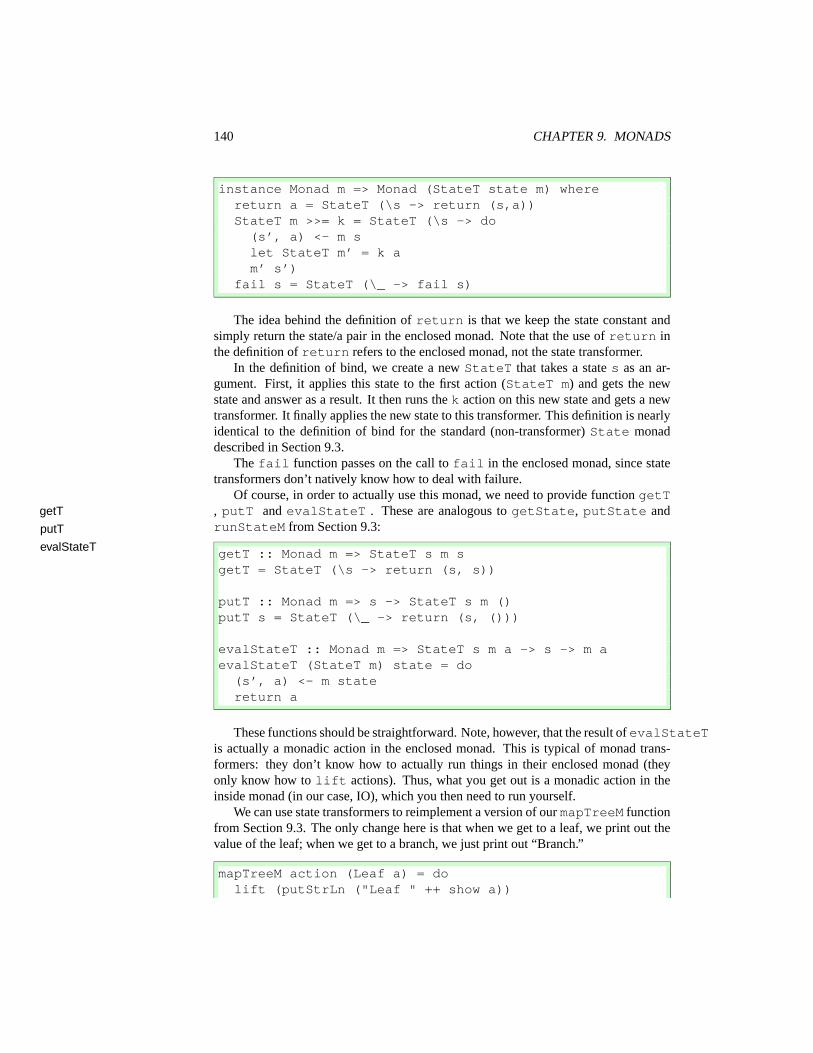
140 CHAPTER 9. MONADS
instance Monad m => Monad (StateT state m) wherereturn a = StateT (\s -> return (s,a))StateT m >>= k = StateT (\s -> do(s’, a) <- m slet StateT m’ = k am’ s’)
fail s = StateT (\_ -> fail s)
The idea behind the definition of return is that we keep the state constant andsimply return the state/a pair in the enclosed monad. Note that the use of return inthe definition of return refers to the enclosed monad, not the state transformer.
In the definition of bind, we create a new StateT that takes a state s as an ar-gument. First, it applies this state to the first action (StateT m) and gets the newstate and answer as a result. It then runs the k action on this new state and gets a newtransformer. It finally applies the new state to this transformer. This definition is nearlyidentical to the definition of bind for the standard (non-transformer) State monaddescribed in Section 9.3.
The fail function passes on the call to fail in the enclosed monad, since statetransformers don’t natively know how to deal with failure.
Of course, in order to actually use this monad, we need to provide function getT, putT and evalStateT . These are analogous to getState, putState andgetT
putT
evalStateT
runStateM from Section 9.3:
getT :: Monad m => StateT s m sgetT = StateT (\s -> return (s, s))
putT :: Monad m => s -> StateT s m ()putT s = StateT (\_ -> return (s, ()))
evalStateT :: Monad m => StateT s m a -> s -> m aevalStateT (StateT m) state = do(s’, a) <- m statereturn a
These functions should be straightforward. Note, however, that the result of evalStateTis actually a monadic action in the enclosed monad. This is typical of monad trans-formers: they don’t know how to actually run things in their enclosed monad (theyonly know how to lift actions). Thus, what you get out is a monadic action in theinside monad (in our case, IO), which you then need to run yourself.
We can use state transformers to reimplement a version of our mapTreeM functionfrom Section 9.3. The only change here is that when we get to a leaf, we print out thevalue of the leaf; when we get to a branch, we just print out “Branch.”
mapTreeM action (Leaf a) = dolift (putStrLn ("Leaf " ++ show a))

9.7. MONAD TRANSFORMERS 141
b <- action areturn (Leaf b)
mapTreeM action (Branch lhs rhs) = dolift (putStrLn "Branch")lhs’ <- mapTreeM action lhsrhs’ <- mapTreeM action rhsreturn (Branch lhs’ rhs’)
The only difference between this function and the one from Section 9.3 is the callsto lift (putStrLn ...) as the first line. The lift tells us that we’re going tobe executing a command in an enclosed monad. In this case, the enclosed monad isIO, since the command lifted is putStrLn.
The type of this function is relatively complex:
mapTreeM :: (MonadTrans t, Monad (t IO), Show a) =>(a -> t IO a1) -> Tree a -> t IO (Tree a1)
Ignoring, for a second, the class constraints, this says that mapTreeM takes anaction and a tree and returns a tree. This just as before. In this, we require that t isa monad transformer (since we apply lift in it); we require that t IO is a monad,since we use putStrLn we know that the enclosed monad is IO; finally, we requirethat a is an instance of show – this is simply because we use show to show the valueof leaves.
Now, we simply change numberTree to use this version of mapTreeM, and thenew versions of get and put, and we end up with:
numberTree tree = mapTreeM number treewhere number v = do
cur <- getTputT (cur+1)return (v,cur)
Using this, we can run our monad:
MTrans> evalStateT (numberTree testTree) 0BranchBranchLeaf ’a’BranchLeaf ’b’Leaf ’c’BranchLeaf ’d’Leaf ’e’*MTrans> it

142 CHAPTER 9. MONADS
Branch (Branch (Leaf (’a’,0))(Branch (Leaf (’b’,1)) (Leaf (’c’,2))))(Branch (Leaf (’d’,3)) (Leaf (’e’,4)))
One problem not specified in our discussion of MonadPlus is that our searchalgorithm will fail to terminate on graphs with cycles. Consider:cycles
gr3 = Graph [(0, ’a’), (1, ’b’), (2, ’c’), (3, ’d’)][(0,1,’l’), (1,0,’m’), (0,2,’n’),(1,3,’o’), (2,3,’p’)]
In this graph, there is a back edge from node b back to node a. If we attempt to runsearchAll2, regardless of what monad we use, it will fail to terminate. Moreover,if we move this erroneous edge to the end of the list (and call this gr4), the result ofsearchAll2 gr4 0 3 will contain an infinite number of paths: presumably weonly want paths that don’t contain cycles.
In order to get around this problem, we need to introduce state. Namely, we needto keep track of which nodes we have visited, so that we don’t visit them again.
We can do this as follows:
searchAll5 g@(Graph vl el) src dst| src == dst = do
visited <- getTputT (src:visited)return [src]
| otherwise = dovisited <- getTputT (src:visited)if src ‘elem‘ visited
then mzeroelse search’ el
wheresearch’ [] = mzerosearch’ ((u,v,_):es)
| src == u =(do path <- searchAll5 g v dst
return (u:path)) ‘mplus‘search’ es
| otherwise = search’ es
Here, we implicitly use a state transformer (see the calls to getT and putT) tokeep track of visited states. We only continue to recurse, when we encounter a state wehaven’t yet visited. Futhermore, when we recurse, we add the current state to our setof visited states.
Now, we can run the state transformer and get out only the correct paths, even onthe cyclic graphs:

9.7. MONAD TRANSFORMERS 143
MTrans> evalStateT (searchAll5 gr3 0 3) [] :: [[Int]][[0,1,3],[0,2,3]]MTrans> evalStateT (searchAll5 gr4 0 3) [] :: [[Int]][[0,1,3],[0,2,3]]
Here, the empty list provided as an argument to evalStateT is the initial state(i.e., the initial visited list). In our case, it is empty.
We can also provide an execStateT method that, instead of returning a result,returns the final state. This function looks like:
execStateT :: Monad m => StateT s m a -> s -> m sexecStateT (StateT m) state = do(s’, a) <- m statereturn s’
This is not so useful in our case, as it will return exactly the reverse of evalStateT(try it and find out!), but can be useful in general (if, for instance, we need to know howmany numbers are used in numberTree).
Exercises
Exercise 9.4 Write a function searchAll6, based on the code for searchAll2,that, at every entry to the main function (not the recursion over the edge list), prints thesearch being conducted. For instance, the output generated for searchAll6 gr 03 should look like:
Exploring 0 -> 3Exploring 1 -> 3Exploring 3 -> 3Exploring 2 -> 3Exploring 3 -> 3MTrans> it[[0,1,3],[0,2,3]]
In order to do this, you will have to define your own list monad transformer and makeappropriate instances of it.
Exercise 9.5 Combine the searchAll5 function (from this section) with the searchAll6function (from the previous exercise) into a single function called searchAll7. Thisfunction should perform IO as in searchAll6 but should also keep track of stateusing a state transformer.

144 CHAPTER 9. MONADS
9.8 Parsing Monads
It turns out that a certain class of parsers are all monads. This makes the constructionof parsing libraries in Haskell very clean. In this chapter, we begin by building our own(small) parsing library in Section 9.8.1 and then introduce the Parsec parsing library inSection 9.8.2.
9.8.1 A Simple Parsing Monad
Consider the task of parsing. A simple parsing monad is much like a state monad,where the state is the unparsed string. We can represent this exactly as:
newtype Parser a = Parser{ runParser :: String -> Either String (String, a) }
We again use Left err to be an error condition. This yields standard instancesof Monad and MonadPlus:
instance Monad Parser wherereturn a = Parser (\xl -> Right (xl,a))fail s = Parser (\xl -> Left s)Parser m >>= k = Parser $ \xl ->case m xl of
Left s -> Left sRight (xl’, a) ->
let Parser n = k ain n xl’
instance MonadPlus Parser wheremzero = Parser (\xl -> Left "mzero")Parser p ‘mplus‘ Parser q = Parser $ \xl ->case p xl of
Right a -> Right aLeft err -> case q xl of
Right a -> Right aLeft _ -> Left err
Now, we want to build up a library of paring “primitives.” The most basic primitiveprimitivesis a parser that will read a specific character. This function looks like:
char :: Char -> Parser Charchar c = Parser char’
where char’ [] = Left ("expecting " ++ show c ++" got EOF")
char’ (x:xs)| x == c = Right (xs, c)
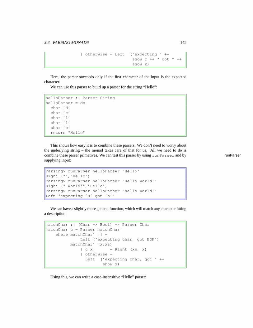
9.8. PARSING MONADS 145
| otherwise = Left ("expecting " ++show c ++ " got " ++show x)
Here, the parser succeeds only if the first character of the input is the expectedcharacter.
We can use this parser to build up a parser for the string “Hello”:
helloParser :: Parser StringhelloParser = dochar ’H’char ’e’char ’l’char ’l’char ’o’return "Hello"
This shows how easy it is to combine these parsers. We don’t need to worry aboutthe underlying string – the monad takes care of that for us. All we need to do iscombine these parser primatives. We can test this parser by using runParser and by runParsersupplying input:
Parsing> runParser helloParser "Hello"Right ("","Hello")Parsing> runParser helloParser "Hello World!"Right (" World!","Hello")Parsing> runParser helloParser "hello World!"Left "expecting ’H’ got ’h’"
We can have a slightly more general function, which will match any character fittinga description:
matchChar :: (Char -> Bool) -> Parser CharmatchChar c = Parser matchChar’
where matchChar’ [] =Left ("expecting char, got EOF")
matchChar’ (x:xs)| c x = Right (xs, x)| otherwise =
Left ("expecting char, got " ++show x)
Using this, we can write a case-insensitive “Hello” parser:

146 CHAPTER 9. MONADS
ciHelloParser = doc1 <- matchChar (‘elem‘ "Hh")c2 <- matchChar (‘elem‘ "Ee")c3 <- matchChar (‘elem‘ "Ll")c4 <- matchChar (‘elem‘ "Ll")c5 <- matchChar (‘elem‘ "Oo")return [c1,c2,c3,c4,c5]
Of course, we could have used something like matchChar ((==’h’) . toLower),but the above implementation works just as well. We can test this function:
Parsing> runParser ciHelloParser "hELlO world!"Right (" world!","hELlO")
Finally, we can have a function, which will match any character:
anyChar :: Parser CharanyChar = Parser anyChar’
where anyChar’ [] =Left ("expecting character, got EOF")
anyChar’ (x:xs) = Right (xs, x)
On top of these primitives, we usually build some combinators. The many combi-manynator, for instance, will take a parser that parses entities of type a and will make it intoa parser that parses entities of type [a] (this is a Kleene-star operator):
many :: Parser a -> Parser [a]many (Parser p) = Parser many’
where many’ xl =case p xl ofLeft err -> Right (xl, [])Right (xl’,a) ->
let Right (xl’’, rest) = many’ xl’in Right (xl’’, a:rest)
The idea here is that first we try to apply the given parser, p. If this fails, we succeedbut return the empty list. If p succeeds, we recurse and keep trying to apply p until itfails. We then return the list of successes we’ve accumulated.
In general, there would be many more functions of this sort, and they would be hid-den away in a library, so that users couldn’t actually look inside the Parser type.However, using them, you could build up, for instance, a parser that parses (non-negative) integers:
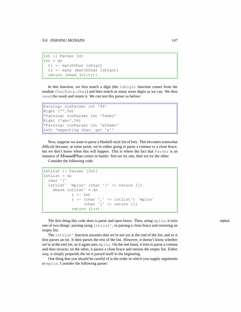
9.8. PARSING MONADS 147
int :: Parser Intint = dot1 <- matchChar isDigittr <- many (matchChar isDigit)return (read (t1:tr))
In this function, we first match a digit (the isDigit function comes from themodule Char/Data.Char) and then match as many more digits as we can. We thenread the result and return it. We can test this parser as before:
Parsing> runParser int "54"Right ("",54)*Parsing> runParser int "54abc"Right ("abc",54)*Parsing> runParser int "a54abc"Left "expecting char, got ’a’"
Now, suppose we want to parse a Haskell-style list of Ints. This becomes somewhatdifficult because, at some point, we’re either going to parse a comma or a close brace,but we don’t know when this will happen. This is where the fact that Parser is aninstance of MonadPlus comes in handy: first we try one, then we try the other.
Consider the following code:
intList :: Parser [Int]intList = dochar ’[’intList’ ‘mplus‘ (char ’]’ >> return [])where intList’ = do
i <- intr <- (char ’,’ >> intList’) ‘mplus‘
(char ’]’ >> return [])return (i:r)
The first thing this code does is parse and open brace. Then, using mplus, it tries mplusone of two things: parsing using intList’, or parsing a close brace and returning anempty list.
The intList’ function assumes that we’re not yet at the end of the list, and so itfirst parses an int. It then parses the rest of the list. However, it doesn’t know whetherwe’re at the end yet, so it again uses mplus. On the one hand, it tries to parse a commaand then recurse; on the other, it parses a close brace and returns the empty list. Eitherway, it simply prepends the int it parsed itself to the beginning.
One thing that you should be careful of is the order in which you supply argumentsto mplus. Consider the following parser:

148 CHAPTER 9. MONADS
tricky =mplus (string "Hal") (string "Hall")
You might expect this parser to parse both the words “Hal” and “Hall;” however, itonly parses the former. You can see this with:
Parsing> runParser tricky "Hal"Right ("","Hal")Parsing> runParser tricky "Hall"Right ("l","Hal")
This is because it tries to parse “Hal,” which succeeds, and then it doesn’t bothertrying to parse “Hall.”
You can attempt to fix this by providing a parser primitive, which detects end-of-file(really, end-of-string) as:
eof :: Parser ()eof = Parser eof’
where eof’ [] = Right ([], ())eof’ xl = Left ("Expecting EOF, got " ++
show (take 10 xl))
You might then rewrite tricky using eof as:
tricky2 = dos <- mplus (string "Hal") (string "Hall")eofreturn s
But this also doesn’t work, as we can easily see:
Parsing> runParser tricky2 "Hal"Right ("",())Parsing> runParser tricky2 "Hall"Left "Expecting EOF, got \"l\""
This is because, again, the mplus doesn’t know that it needs to parse the wholeinput. So, when you provide it with “Hall,” it parses just “Hal” and leaves the last “l”lying around to be parsed later. This causes eof to produce an error message.
The correct way to implement this is:
tricky3 =mplus (do s <- string "Hal"

9.8. PARSING MONADS 149
eofreturn s)
(do s <- string "Hall"eofreturn s)
We can see that this works:
Parsing> runParser tricky3 "Hal"Right ("","Hal")Parsing> runParser tricky3 "Hall"Right ("","Hall")
This works precisely because each side of the mplus knows that it must read theend.
In this case, fixing the parser to accept both “Hal” and “Hall” was fairly simple,due to the fact that we assumed we would be reading an end-of-file immediately af-terwards. Unfortunately, if we cannot disambiguate immediately, life becomes signifi-cantly more complicated. This is a general problem in parsing, and has little to do withmonadic parsing. The solution most parser libraries (e.g., Parsec, see Section 9.8.2)have adopted is to only recognize “LL(1)” grammars: that means that you must be ableto disambiguate the input with a one token look-ahead.
ExercisesExercise 9.6 Write a parser intListSpace that will parse int lists but will allowarbitrary white space (spaces, tabs or newlines) between the commas and brackets.
Given this monadic parser, it is fairly easy to add information regarding sourceposition. For instance, if we’re parsing a large file, it might be helpful to report theline number on which an error occurred. We could do this simply by extending the line numbersParser type and by modifying the instances and the primitives:
newtype Parser a = Parser{ runParser :: Int -> String ->
Either String (Int, String, a) }
instance Monad Parser wherereturn a = Parser (\n xl -> Right (n,xl,a))fail s = Parser (\n xl -> Left (show n ++
": " ++ s))Parser m >>= k = Parser $ \n xl ->case m n xl of
Left s -> Left sRight (n’, xl’, a) ->
let Parser m2 = k a

150 CHAPTER 9. MONADS
in m2 n’ xl’
instance MonadPlus Parser wheremzero = Parser (\n xl -> Left "mzero")Parser p ‘mplus‘ Parser q = Parser $ \n xl ->case p n xl ofRight a -> Right aLeft err -> case q n xl of
Right a -> Right aLeft _ -> Left err
matchChar :: (Char -> Bool) -> Parser CharmatchChar c = Parser matchChar’where matchChar’ n [] =
Left ("expecting char, got EOF")matchChar’ n (x:xs)
| c x =Right (n+if x==’\n’ then 1 else 0
, xs, x)| otherwise =
Left ("expecting char, got " ++show x)
The definitions for char and anyChar are not given, since they can be written interms of matchChar. The many function needs to be modified only to include thenew state.
Now, when we run a parser and there is an error, it will tell us which line numbercontains the error:
Parsing2> runParser helloParser 1 "Hello"Right (1,"","Hello")Parsing2> runParser int 1 "a54"Left "1: expecting char, got ’a’"Parsing2> runParser intList 1 "[1,2,3,a]"Left "1: expecting ’]’ got ’1’"
We can use the intListSpace parser from the prior exercise to see that this doesin fact work:
Parsing2> runParser intListSpace 1"[1 ,2 , 4 \n\n ,a\n]"
Left "3: expecting char, got ’a’"Parsing2> runParser intListSpace 1
"[1 ,2 , 4 \n\n\n ,a\n]"Left "4: expecting char, got ’a’"Parsing2> runParser intListSpace 1

9.8. PARSING MONADS 151
"[1 ,\n2 , 4 \n\n\n ,a\n]"Left "5: expecting char, got ’a’"
We can see that the line number, on which the error occurs, increases as we addadditional newlines before the erroneous “a”.
9.8.2 Parsec
As you continue developing your parser, you might want to add more and more fea-tures. Luckily, Graham Hutton and Daan Leijen have already done this for us in theParsec library. This section is intended to be an introduction to the Parsec library; it byno means covers the whole library, but it should be enough to get you started.
Like our libarary, Parsec provides a few basic functions to build parsers from char-acters. These are: char, which is the same as our char; anyChar, which is the same char
anyCharas our anyChar; satisfy, which is the same as our matchChar; oneOf, whichsatisfy
oneOf
takes a list of Chars and matches any of them; and noneOf, which is the opposite of
noneOf
oneOf.The primary function Parsec uses to run a parser is parse. However, in addition to
parsea parser, this function takes a string that represents the name of the file you’re parsing.This is so it can give better error messages. We can try parsing with the above functions:
ParsecI> parse (char ’a’) "stdin" "a"Right ’a’ParsecI> parse (char ’a’) "stdin" "ab"Right ’a’ParsecI> parse (char ’a’) "stdin" "b"Left "stdin" (line 1, column 1):unexpected "b"expecting "a"ParsecI> parse (char ’H’ >> char ’a’ >> char ’l’)
"stdin" "Hal"Right ’l’ParsecI> parse (char ’H’ >> char ’a’ >> char ’l’)
"stdin" "Hap"Left "stdin" (line 1, column 3):unexpected "p"expecting "l"
Here, we can see a few differences between our parser and Parsec: first, the restof the string isn’t returned when we run parse. Second, the error messages producedare much better.
In addition to the basic character parsing functions, Parsec provides primitives for:spaces, which is the same as ours; space which parses a single space; letter, spaces
space
letter
which parses a letter; digit, which parses a digit; string, which is the same as
digit
string
ours; and a few others.We can write our int and intList functions in Parsec as:

152 CHAPTER 9. MONADS
int :: CharParser st Intint = doi1 <- digitir <- many digitreturn (read (i1:ir))
intList :: CharParser st [Int]intList = dochar ’[’intList’ ‘mplus‘ (char ’]’ >> return [])where intList’ = do
i <- intr <- (char ’,’ >> intList’) ‘mplus‘
(char ’]’ >> return [])return (i:r)
First, note the type signatures. The st type variable is simply a state variable thatwe are not using. In the int function, we use the many function (built in to Parsec)together with the digit function (also built in to Parsec). The intList function isactually identical to the one we wrote before.
Note, however, that using mplus explicitly is not the preferred method of com-bining parsers: Parsec provides a <|> function that is a synonym of mplus, but thatlooks nicer:
intList :: CharParser st [Int]intList = dochar ’[’intList’ <|> (char ’]’ >> return [])where intList’ = do
i <- intr <- (char ’,’ >> intList’) <|>
(char ’]’ >> return [])return (i:r)
We can test this:
ParsecI> parse intList "stdin" "[3,5,2,10]"Right [3,5,2,10]ParsecI> parse intList "stdin" "[3,5,a,10]"Left "stdin" (line 1, column 6):unexpected "a"expecting digit
In addition to these basic combinators, Parsec provides a few other useful ones:

9.8. PARSING MONADS 153
• choice takes a list of parsers and performs an or operation (<|>) between allof them.
• option takes a default value of type a and a parser that returns something oftype a. It then tries to parse with the parser, but it uses the default value as thereturn, if the parsing fails.
• optional takes a parser that returns () and optionally runs it.
• between takes three parsers: an open parser, a close parser and a betweenparser. It runs them in order and returns the value of the between parser. Thiscan be used, for instance, to take care of the brackets on our intList parser.
• notFollowedBy takes a parser and returns one that succeeds only if the givenparser would have failed.
Suppose we want to parse a simple calculator language that includes only plusand times. Furthermore, for simplicity, assume each embedded expression must beenclosed in parentheses. We can give a datatype for this language as:
data Expr = Value Int| Expr :+: Expr| Expr :*: Exprderiving (Eq, Ord, Show)
And then write a parser for this language as:
parseExpr :: Parser ExprparseExpr = choice[ do i <- int; return (Value i), between (char ’(’) (char ’)’) $ do
e1 <- parseExprop <- oneOf "+*"e2 <- parseExprcase op of’+’ -> return (e1 :+: e2)’*’ -> return (e1 :*: e2)
]
Here, the parser alternates between two options (we could have used <|>, but Iwanted to show the choice combinator in action). The first simply parses an int andthen wraps it up in the Value constructor. The second option uses between to parsetext between parentheses. What it parses is first an expression, then one of plus ortimes, then another expression. Depending on what the operator is, it returns either e1:+: e2 or e1 :*: e2.
We can modify this parser, so that instead of computing an Expr, it simply com-putes the value:
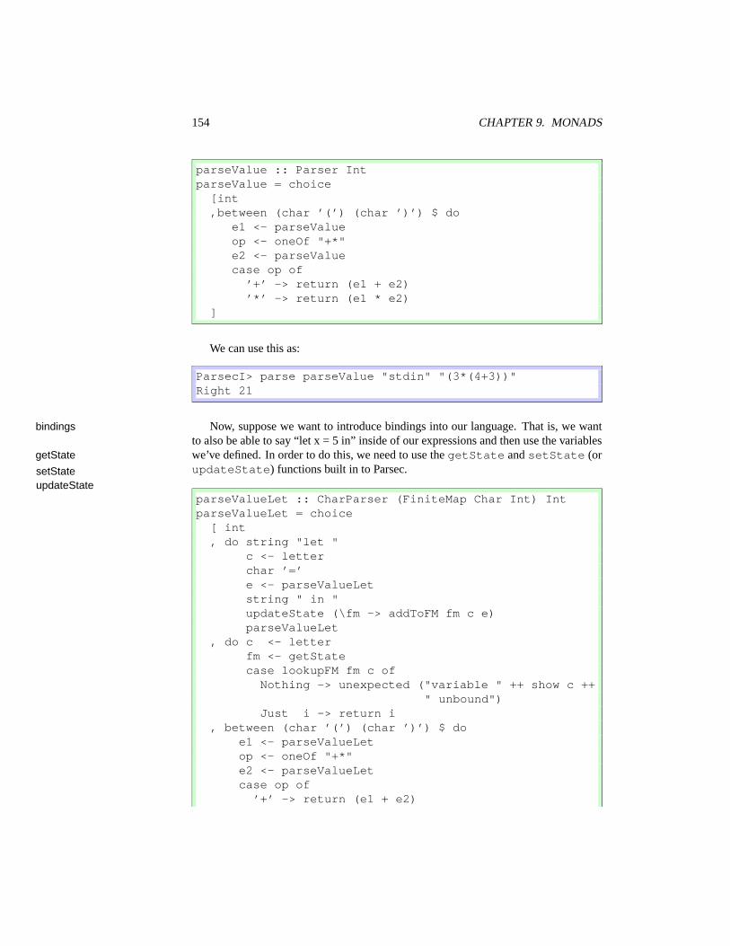
154 CHAPTER 9. MONADS
parseValue :: Parser IntparseValue = choice[int,between (char ’(’) (char ’)’) $ do
e1 <- parseValueop <- oneOf "+*"e2 <- parseValuecase op of
’+’ -> return (e1 + e2)’*’ -> return (e1 * e2)
]
We can use this as:
ParsecI> parse parseValue "stdin" "(3*(4+3))"Right 21
Now, suppose we want to introduce bindings into our language. That is, we wantbindingsto also be able to say “let x = 5 in” inside of our expressions and then use the variableswe’ve defined. In order to do this, we need to use the getState and setState (orgetState
setState updateState) functions built in to Parsec.updateState
parseValueLet :: CharParser (FiniteMap Char Int) IntparseValueLet = choice[ int, do string "let "
c <- letterchar ’=’e <- parseValueLetstring " in "updateState (\fm -> addToFM fm c e)parseValueLet
, do c <- letterfm <- getStatecase lookupFM fm c ofNothing -> unexpected ("variable " ++ show c ++
" unbound")Just i -> return i
, between (char ’(’) (char ’)’) $ doe1 <- parseValueLetop <- oneOf "+*"e2 <- parseValueLetcase op of
’+’ -> return (e1 + e2)

9.8. PARSING MONADS 155
’*’ -> return (e1 * e2)]
The int and recursive cases remain the same. We add two more cases, one to dealwith let-bindings, the other to deal with usages.
In the let-bindings case, we first parse a “let” string, followed by the character we’rebinding (the letter function is a Parsec primitive that parses alphabetic characters),followed by it’s value (a parseValueLet). Then, we parse the “ in ” and update thestate to include this binding. Finally, we continue and parse the rest.
In the usage case, we simply parse the character and then look it up in the state.However, if it doesn’t exist, we use the Parsec primitive unexpected to report anerror.
We can see this parser in action using the runParser command, which enables runParserus to provide an initial state:
ParsecI> runParser parseValueLet emptyFM "stdin""let c=5 in ((5+4)*c)"
Right 45*ParsecI> runParser parseValueLet emptyFM "stdin"
"let c=5 in ((5+4)*let x=2 in (c+x))"Right 63*ParsecI> runParser parseValueLet emptyFM "stdin"
"((let x=2 in 3+4)*x)"Right 14
Note that the bracketing does not affect the definitions of the variables. For in-stance, in the last example, the use of “x” is, in some sense, outside the scope of thedefinition. However, our parser doesn’t notice this, since it operates in a strictly left-to-right fashion. In order to fix this omission, bindings would have to be removed (seethe exercises).
ExercisesExercise 9.7 Modify the parseValueLet parser, so that it obeys bracketing. Inorder to do this, you will need to change the state to something like FiniteMapChar [Int], where the [Int] is a stack of definitions.

156 CHAPTER 9. MONADS

Chapter 10
Advanced Techniques
10.1 Exceptions
10.2 Mutable Arrays
10.3 Mutable References
10.4 The ST Monad
10.5 Concurrency
10.6 Regular Expressions
10.7 Dynamic Types
157

158 CHAPTER 10. ADVANCED TECHNIQUES
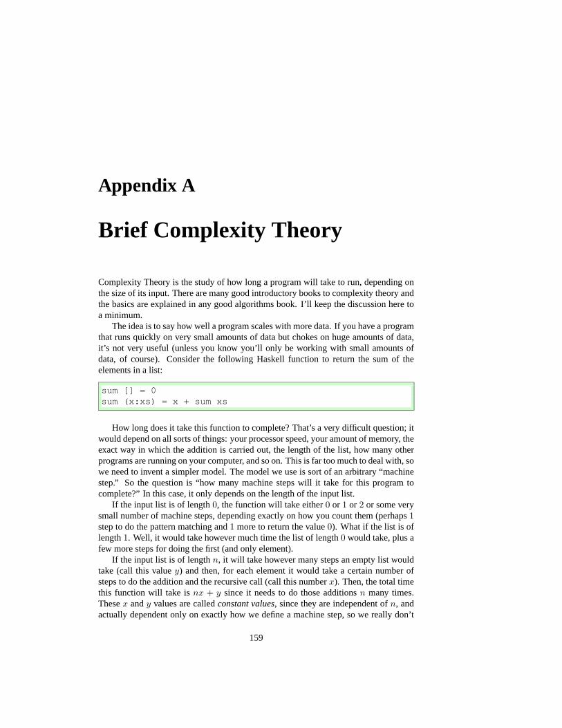
Appendix A
Brief Complexity Theory
Complexity Theory is the study of how long a program will take to run, depending onthe size of its input. There are many good introductory books to complexity theory andthe basics are explained in any good algorithms book. I’ll keep the discussion here toa minimum.
The idea is to say how well a program scales with more data. If you have a programthat runs quickly on very small amounts of data but chokes on huge amounts of data,it’s not very useful (unless you know you’ll only be working with small amounts ofdata, of course). Consider the following Haskell function to return the sum of theelements in a list:
sum [] = 0sum (x:xs) = x + sum xs
How long does it take this function to complete? That’s a very difficult question; itwould depend on all sorts of things: your processor speed, your amount of memory, theexact way in which the addition is carried out, the length of the list, how many otherprograms are running on your computer, and so on. This is far too much to deal with, sowe need to invent a simpler model. The model we use is sort of an arbitrary “machinestep.” So the question is “how many machine steps will it take for this program tocomplete?” In this case, it only depends on the length of the input list.
If the input list is of length 0, the function will take either 0 or 1 or 2 or some verysmall number of machine steps, depending exactly on how you count them (perhaps 1step to do the pattern matching and 1 more to return the value 0). What if the list is oflength 1. Well, it would take however much time the list of length 0 would take, plus afew more steps for doing the first (and only element).
If the input list is of length n, it will take however many steps an empty list wouldtake (call this value y) and then, for each element it would take a certain number ofsteps to do the addition and the recursive call (call this number x). Then, the total timethis function will take is nx + y since it needs to do those additions n many times.These x and y values are called constant values, since they are independent of n, andactually dependent only on exactly how we define a machine step, so we really don’t
159
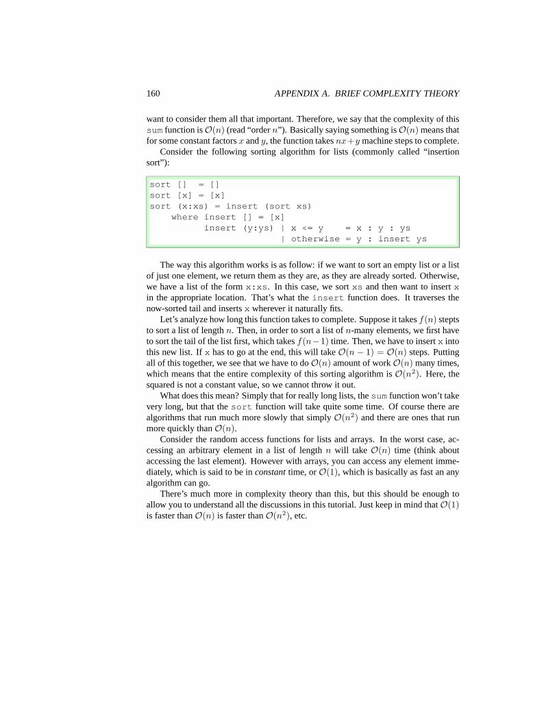
160 APPENDIX A. BRIEF COMPLEXITY THEORY
want to consider them all that important. Therefore, we say that the complexity of thissum function is O(n) (read “order n”). Basically saying something is O(n) means thatfor some constant factors x and y, the function takes nx+y machine steps to complete.
Consider the following sorting algorithm for lists (commonly called “insertionsort”):
sort [] = []sort [x] = [x]sort (x:xs) = insert (sort xs)
where insert [] = [x]insert (y:ys) | x <= y = x : y : ys
| otherwise = y : insert ys
The way this algorithm works is as follow: if we want to sort an empty list or a listof just one element, we return them as they are, as they are already sorted. Otherwise,we have a list of the form x:xs. In this case, we sort xs and then want to insert xin the appropriate location. That’s what the insert function does. It traverses thenow-sorted tail and inserts x wherever it naturally fits.
Let’s analyze how long this function takes to complete. Suppose it takes f(n) steptsto sort a list of length n. Then, in order to sort a list of n-many elements, we first haveto sort the tail of the list first, which takes f(n−1) time. Then, we have to insert x intothis new list. If x has to go at the end, this will take O(n − 1) = O(n) steps. Puttingall of this together, we see that we have to do O(n) amount of work O(n) many times,which means that the entire complexity of this sorting algorithm is O(n2). Here, thesquared is not a constant value, so we cannot throw it out.
What does this mean? Simply that for really long lists, the sum function won’t takevery long, but that the sort function will take quite some time. Of course there arealgorithms that run much more slowly that simply O(n2) and there are ones that runmore quickly than O(n).
Consider the random access functions for lists and arrays. In the worst case, ac-cessing an arbitrary element in a list of length n will take O(n) time (think aboutaccessing the last element). However with arrays, you can access any element imme-diately, which is said to be in constant time, or O(1), which is basically as fast an anyalgorithm can go.
There’s much more in complexity theory than this, but this should be enough toallow you to understand all the discussions in this tutorial. Just keep in mind that O(1)is faster than O(n) is faster than O(n2), etc.

Appendix B
Recursion and Induction
Informally, a function is recursive if its definition depends on itself. The prototypicalexample is factorial, whose definition is:
fact(n) =
{
1 n = 0n ∗ fact(n − 1) n > 0
Here, we can see that in order to calculate fact(5), we need to calculate fact(4),but in order to calculatefact(4), we need to calculate fact(3), and so on.
Recursive function definitions always contain a number of non-recursive base casesand a number of recursive cases. In the case of factorial, we have one of each. Thebase case is when n = 0 and the recursive case is when n > 0.
One can actually think of the natural numbers themselves as recursive (in fact, ifyou ask set theorists about this, they’ll say this is how it is). That is, there is a zeroelement and then for every element, it has a successor. That is 1 = succ(0), 2 =succ(1), . . . , 573 = succ(573), . . . and so on forever. We can actually implement thissystem of natural numbers in Haskell:
data Nat = Zero | Succ Nat
This is a recursive type definition. Here, we represent one as Succ Zero andthree as Succ (Succ (Succ Zero)). One thing we might want to do is be ableto convert back and forth beween Nats and Ints. Clearly, we can write a base case as:
natToInt Zero = 0
In order to write the recursive case, we realize that we’re going to have somethingof the form Succ n. We can make the assumption that we’ll be able to take n andproduce an Int. Assuming we can do this, all we need to do is add one to this result.This gives rise to our recursive case:
natToInt (Succ n) = natToInt n + 1
161

162 APPENDIX B. RECURSION AND INDUCTION
There is a close connection between recursion and mathematical induction. Induc-tion is a proof technique which typically breaks problems down into base cases and“inductive” cases, very analogous to our analysis of recursion.
Let’s say we want to prove the statement n! ≥ n for all n ≥ 0. First we formulatea base case: namely, we wish to prove the statement when n = 0. When n = 0, n! = 1by definition. Since n! = 1 > 0 = n, we get that 0! ≥ 0 as desired.
Now, suppose that n > 0. Then n = k + 1 for some value k. We now invoke theinductive hypothesis and claim that the statement holds for n = k. That is, we assumethat k! ≥ k. Now, we use k to formate the statement for our value of n. That is, n! ≥ nif and only iff (k + 1)! ≥ (k + 1). We now apply the definition of factorial and get(k + 1)! = (k + 1) ∗ k!. Now, we know k! ≥ k, so (k + 1) ∗ k! ≥ k + 1 if and only ifk + 1 ≥ 1. But we know that k ≥ 0, which means k + 1 ≥ 1. Thus it is proven.
It may seem a bit counter-intuitive that we are assuming that the claim is true for kin our proof that it is true for n. You can think of it like this: we’ve proved the statementfor the case when n = 0. Now, we know it’s true for n = 0 so using this we use ourinductive argument to show that it’s true for n = 1. Now, we know that it is true forn = 1 so we reuse our inductive argument to show that it’s true for n = 2. We cancontinue this argument as long as we want and then see that it’s true for all n.
It’s much like pushing down dominoes. You know that when you push down thefirst domino, it’s going to knock over the second one. This, in turn will knock over thethird, and so on. The base case is like pushing down the first domino, and the inductivecase is like showing that pushing down domino k will cause the k + 1st domino to fall.
In fact, we can use induction to prove that our natToInt function does the rightthing. First we prove the base case: does natToInt Zero evaluate to 0? Yes, obvi-ously it does. Now, we can assume that natToInt n evaluates to the correct value(this is the inductive hypothesis) and ask whether natToInt (Succ n) producesthe correct value. Again, it is obvious that it does, by simply looking at the definition.
Let’s consider a more complex example: addition of Nats. We can write this con-cisely as:
addNat Zero m = maddNat (Succ n) m = addNat n (Succ m)
Now, let’s prove that this does the correct thing. First, as the base case, suppose thefirst argument is Zero. We know that 0 + m = m regardless of what m is; thus in thebase case the algorithm does the correct thing. Now, suppose that addNat n m doesthe correct thing for all m and we want to show that addNat (Succ n) m does thecorrect thing. We know that (n + 1) + m = n + (m + 1) and thus since addNatn (Succ m) does the correct thing (by the inductive hypothesis), our program iscorrect.

Appendix C
Solutions To Exercises
Solution 3.1It binds more tightly; actually, function application binds more tightly than anythingelse. To see this, we can do something like:
Prelude> sqrt 3 * 35.19615
If multiplication bound more tightly, the result would have been 3.
Solution 3.2Solution: snd (fst ((1,’a’),"foo")). This is because first we want to takethe first half the the tuple: (1,’a’) and then out of this we want to take the secondhalf, yielding just ’a’.
If you tried fst (snd ((1,’a’),"foo")) you will have gotten a type error.This is because the application of snd will leave you with fst "foo". However, thestring “foo” isn’t a tuple, so you cannot apply fst to it.
Solution 3.3Solution: map Char.isLower ”aBCde”
Solution 3.4Solution: length (filter Char.isLower ”aBCde”)
Solution 3.5foldr max 0 [5,10,2,8,1]. You could also use foldl. The foldr case is easier to explain:we replace each cons with an application of max and the empty list with 0. Thus, theinner-most application will take the maximum of 0 and the last element of the list (ifit exists). Then, the next-most inner application will return the maximum of what-ever was the maximum before and the second-to-last element. This will continue on,carrying to current maximum all the way back to the beginning of the list.
163

164 APPENDIX C. SOLUTIONS TO EXERCISES
In the foldl case, we can think of this as looking at each element in the list in order.We start off our “state” with 0. We pull off the first element and check to see if it’sbigger than our current state. If it is, we replace our current state with that number andthe continue. This happens for each element and thus eventually returns the maximalelement.
Solution 3.6fst (head (tail [(5,’b’),(1,’c’),(6,’a’)]))
Solution 3.7We can define a fibonacci function as:
fib 1 = 1fib 2 = 1fib n = fib (n-1) + fib (n-2)
We could also write it using explicit if statements, like:
fib n =if n == 1 || n == 2then 1else fib (n-1) + fib (n-2)
Either is acceptable, but the first is perhaps more natural in Haskell.
Solution 3.8We can define:
a ∗ b =
{
a b = 1a + a ∗ (b − 1) otherwise
And then type out code:
mult a 1 = amult a b = a + mult a (b-1)
Note that it doesn’t matter that of a and b we do the recursion on. We could just aswell have defined it as:
mult 1 b = bmult a b = b + mult (a-1) b
Solution 3.9We can define my map as:

165
my_map f [] = []my_map f (x:xs) = f x : my_map f xs
Recall that the my map function is supposed to apply a function f to every elementin the list. In the case that the list is empty, there are no elements to apply the functionto, so we just return the empty list.
In the case that the list is non-empty, it is an element x followed by a list xs.Assuming we’ve already properly applied my map to xs, then all we’re left to do isapply f to x and then stick the results together. This is exactly what the second linedoes.
Solution 3.10The code below appears in Numbers.hs. The only tricky parts are the recursive callsin getNums and showFactorials.
module Mainwhere
import IO
main = donums <- getNumsputStrLn ("The sum is " ++ show (sum nums))putStrLn ("The product is " ++ show (product nums))showFactorials nums
getNums = doputStrLn "Give me a number (or 0 to stop):"num <- getLineif read num == 0then return []else do rest <- getNums
return ((read num :: Int):rest)
showFactorials [] = return ()showFactorials (x:xs) = doputStrLn (show x ++ " factorial is " ++
show (factorial x))showFactorials xs
factorial 1 = 1factorial n = n * factorial (n-1)
The idea for getNums is just as spelled out in the hint. For showFactorials,we consider first the recursive call. Suppose we have a list of numbers, the first of

166 APPENDIX C. SOLUTIONS TO EXERCISES
which is x. First we print out the string showing the factorial. Then we print out therest, hence the recursive call. But what should we do in the case of the empty list?Clearly we are done, so we don’t need to do anything at all, so we simply return().
Note that this must be return () instead of just () because if we simply wroteshowFactorials [] = () then this wouldn’t be an IO action, as it needs to be.For more clarification on this, you should probably just keep reading the tutorial.
Solution 4.1 1.
String or [Char]
2. type error: lists are homogenous
3. Num a ⇒ (a,Char)
4. Int
5. type error: cannot add values of different types
Solution 4.2The types:
1. (a, b)− > b
2. [a]− > a
3. [a]− > Bool
4. [a]− > a
5. [[a]]− > a
Solution 4.3The types:
1. a− > [a]. This function takes an element and returns the list containing only thatelement.
2. a− > b− > b− > (a, [b]). The second and third argument must be of the sametype, since they go into the same list. The first element can be of any type.
3. Num a => a− > a. Since we apply (+) to a, it must be an instance of Num.
4. a− > String. This ignores the first argument, so it can be any type.
5. (Char− > a)− > a. In this expression, x must be a function which takes a Char
as an argument. We don’t know anything about what it produces, though, so wecall it a.

167
6. Type error. Here, we assume x has type a. But x is applied to itself, so it musthave type b− > c. But then it must have type (b− > c)− > c, but then it musthave type ((b− > c)− > c)− > c and so on, leading to an infinite type.
7. Num a => a− > a. Again, since we apply (+), this must be an instance ofNum.
Solution 4.4The definitions will be something like:
data Triple a b c = Triple a b c
tripleFst (Triple x y z) = xtripleSnd (Triple x y z) = ytripleThr (Triple x y z) = z
Solution 4.5The code, with type signatures, is:
data Quadruple a b = Quadruple a a b b
firstTwo :: Quadruple a b -> [a]firstTwo (Quadruple x y z t) = [x,y]
lastTwo :: Quadruple a b -> [b]lastTwo (Quadruple x y z t) = [z,t]
We note here that there are only two type variables, a and b associated withQuadruple.
Solution 4.6The code:
data Tuple a b c d e = One a| Two a b| Three a b c| Four a b c d
tuple1 (One a ) = Just atuple1 (Two a b ) = Just atuple1 (Three a b c ) = Just atuple1 (Four a b c d) = Just a
tuple2 (One a ) = Nothingtuple2 (Two a b ) = Just btuple2 (Three a b c ) = Just b

168 APPENDIX C. SOLUTIONS TO EXERCISES
tuple2 (Four a b c d) = Just b
tuple3 (One a ) = Nothingtuple3 (Two a b ) = Nothingtuple3 (Three a b c ) = Just ctuple3 (Four a b c d) = Just c
tuple4 (One a ) = Nothingtuple4 (Two a b ) = Nothingtuple4 (Three a b c ) = Nothingtuple4 (Four a b c d) = Just d
Solution 4.7The code:
fromTuple (One a ) = Left (Left a )fromTuple (Two a b ) = Left (Right (a,b) )fromTuple (Three a b c ) = Right (Left (a,b,c) )fromTuple (Four a b c d) = Right (Right (a,b,c,d))
Here, we use embedded Eithers to represent the fact that there are four (insteadof two) options.
Solution 4.8The code:
listHead (Cons x xs) = xlistTail (Cons x xs) = xs
listFoldl f y Nil = ylistFoldl f y (Cons x xs) = listFoldl f (f y x) xs
listFoldr f y Nil = ylistFoldr f y (Cons x xs) = f x (foldr f z xs)
Solution 4.9The code:
elements (Leaf x) = [x]elements (Branch lhs x rhs) =elements lhs ++ [x] ++ elements rhs
Solution 4.10The code:

169
foldTree :: (a -> b -> b) -> b -> BinaryTree a -> bfoldTree f z (Leaf x) = f x zfoldTree f z (Branch lhs x rhs) =
foldTree f (f x (foldTree f z rhs)) lhs
elements2 = foldTree (:) []
or:
elements2 tree = foldTree (\a b -> a:b) [] tree
The first elements2 is simply a more compact version of the second.
Solution 4.11It mimicks neither exactly. It’s behavior most closely resembles foldr, but differsslightly in its treatment of the initial value. We can observe the difference in an inter-preter:
CPS> foldr (-) 0 [1,2,3]2CPS> foldl (-) 0 [1,2,3]-6CPS> fold (-) 0 [1,2,3]-2
Clearly it behaves differently. By writing down the derivations of fold and foldrwe can see exactly where they diverge:
foldr (-) 0 [1,2,3]==> 1 - foldr (-) 0 [2,3]==> ...==> 1 - (2 - (3 - foldr (-) 0 []))==> 1 - (2 - (3 - 0))==> 2
fold (-) 0 [1,2,3]==> fold’ (-) (\y -> 0 - y) [1,2,3]==> 0 - fold’ (-) (\y -> 1 - y) [2,3]==> 0 - (1 - fold’ (-) (\y -> 2 - y) [3])==> 0 - (1 - (2 - 3))==> -2
Essentially, the primary difference is that in the foldr case, the “initial value” isused at the end (replacing []), whereas in the CPS case, the initial value is used at thebeginning.

170 APPENDIX C. SOLUTIONS TO EXERCISES
Solution 4.12
Solution 5.1Using if, we get something like:
main = doputStrLn "Please enter your name:"name <- getLineif name == "Simon" || name == "John" || name == "Phil"then putStrLn "Haskell is great!"else if name == "Koen"
then putStrLn "Debugging Haskell is fun!"else putStrLn "I don’t know who you are."
Note that we don’t need to repeat the dos inside the ifs, since these are only oneaction commands.
We could also be a bit smarter and use the elem command which is built in to thePrelude:
main = doputStrLn "Please enter your name:"name <- getLineif name ‘elem‘ ["Simon", "John", "Phil"]then putStrLn "Haskell is great!"else if name == "Koen"
then putStrLn "Debugging Haskell is fun!"else putStrLn "I don’t know who you are."
Of course, we needn’t put all the putStrLns inside the if statements. We couldinstead write:
main = doputStrLn "Please enter your name:"name <- getLineputStrLn(if name ‘elem‘ ["Simon", "John", "Phil"]
then "Haskell is great!"else if name == "Koen"
then "Debugging Haskell is fun!"else "I don’t know who you are.")
Using case, we get something like:
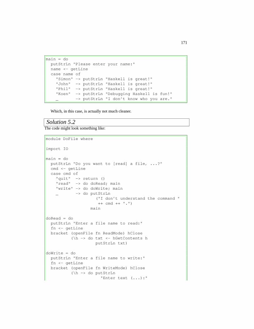
171
main = doputStrLn "Please enter your name:"name <- getLinecase name of"Simon" -> putStrLn "Haskell is great!""John" -> putStrLn "Haskell is great!""Phil" -> putStrLn "Haskell is great!""Koen" -> putStrLn "Debugging Haskell is fun!"_ -> putStrLn "I don’t know who you are."
Which, in this case, is actually not much cleaner.
Solution 5.2The code might look something like:
module DoFile where
import IO
main = doputStrLn "Do you want to [read] a file, ...?"cmd <- getLinecase cmd of"quit" -> return ()"read" -> do doRead; main"write" -> do doWrite; main_ -> do putStrLn
("I don’t understand the command "++ cmd ++ ".")
main
doRead = doputStrLn "Enter a file name to read:"fn <- getLinebracket (openFile fn ReadMode) hClose
(\h -> do txt <- hGetContents hputStrLn txt)
doWrite = doputStrLn "Enter a file name to write:"fn <- getLinebracket (openFile fn WriteMode) hClose
(\h -> do putStrLn"Enter text (...):"

172 APPENDIX C. SOLUTIONS TO EXERCISES
writeLoop h)
writeLoop h = dol <- getLineif l == "."then return ()else do hPutStrLn h l
writeLoop h
The only interesting things here are the calls to bracket, which ensure the that theprogram lives on, regardless of whether there’s a failure or not; and the writeLoopfunction. Note that we need to pass the handle returned by openFile (throughbracket to this function, so it knows where to write the input to).
Solution 7.1Function func3 cannot be converted into point-free style. The others look somethinglike:
func1 x = map (*x)
func2 f g = filter f . map g
func4 = map (+2) . filter (‘elem‘ [1..10]) . (5:)
func5 = foldr (uncurry $ flip f) 0
You might have been tempted to try to write func2 as filter f . map,trying to eta-reduce off the g. In this case, this isn’t possible. This is because thefunction composition operator (.) has type (b → c) → (a → b) → (a → c). In thiscase, we’re trying to use map as the second argument. But map takes two arguments,while (.) expects a function which takes only one.
Solution 7.2We can start out with a recursive definition:
and [] = Trueand (x:xs) = x && and xs
From here, we can clearly rewrite this as:
and = foldr (&&) True
Solution 7.3We can write this recursively as:

173
concatMap f [] = []concatMap f (x:xs) = f x ++ concatMap f xs
This hints that we can write this as:
concatMap f = foldr (\a b -> f a ++ b) []
Now, we can do point elimination to get:
foldr (\a b -> f a ++ b) []==> foldr (\a b -> (++) (f a) b) []==> foldr (\a -> (++) (f a)) []==> foldr (\a -> ((++) . f) a) []==> foldr ((++) . f) []
Solution 9.1The first law is: return a >>= f ≡ f a. In the case of Maybe, we get:
return a >>= f==> Just a >>= \x -> f x==> (\x -> f x) a==> f a
The second law is: f >>= return ≡ f. Here, we get:
f >>= return==> f >>= \x -> return x==> f >>= \x -> Just x
At this point, there are two cases depending on whether f is Nothing or not. Inthe first case, we get:
==> Nothing >>= \x -> Just x==> Nothing==> f
In the second case, f is Just a. Then, we get:
==> Just a >>= \x -> Just x==> (\x -> Just x) a==> Just a==> f

174 APPENDIX C. SOLUTIONS TO EXERCISES
And the second law is shown. The third law states: f >>= (\x -> g x >>=h) ≡ (f >>= g) >>= h.
If f is Nothing, then the left-hand-side clearly reduces to Nothing. The right-hand-side reduces to Nothing >>= h which in turn reduces to Nothing, so theyare the same.
Suppose f is Just a. Then the LHS reduces to g a >>= h and the RHS re-duces to (Just a >>= \x -> g x) >>= h which in turn reduces to g a >>=h, so these two are the same.
Solution 9.2The idea is that we wish to use the Left constructor to represent errors on the Rightconstructor to represent successes. This leads to an instance declaration like:
instance Monad (Either String) wherereturn x = Right xLeft s >>= _ = Left sRight x >>= f = f xfail s = Left s
If we try to use this monad to do search, we get:
Monads> searchAll gr 0 3 :: Either String [Int]Right [0,1,3]Monads> searchAll gr 3 0 :: Either String [Int]Left "no path"
which is exactly what we want.
Solution 9.3The order to mplus essentially determins the search order. When the recursive call tosearchAll2 comes first, we are doing depth-first search. When the recursive call tosearch’ comes first, we are doing breadth-first search. Thus, using the list monad,we expect the solutions to come in the other order:
MPlus> searchAll3 gr 0 3 :: [[Int]][[0,2,3],[0,1,3]]
Just as we expected.
Solution 9.4This is a very difficult problem; if you found that you were stuck immediately, pleasejust read as much of this solution as you need to try it yourself.
First, we need to define a list transformer monad. This looks like:

175
newtype ListT m e = ListT { unListT :: m [e] }
The ListT constructor simply wraps a monadic action (in monad m) which returnsa list.
We now need to make this a monad:
instance Monad m => Monad (ListT m) wherereturn x = ListT (return [x])fail s = ListT (return [] )ListT m >>= k = ListT $ do
l <- ml’ <- mapM (unListT . k) lreturn (concat l’)
Here, success is designated by a monadic action which returns a singleton list.Failure (like in the standard list monad) is represented by an empty list: of course, it’sactually an empty list returned from the enclosed monad. Binding happens essentiallyby running the action which will result in a list l. This has type [e]. We now needto apply k to each of these elements (which will result in something of type ListT m[e2]. We need to get rid of the ListTs around this (by using unListT) and thenconcatenate them to make a single list.
Now, we need to make it an instance of MonadPlus
instance Monad m => MonadPlus (ListT m) wheremzero = ListT (return [])ListT m1 ‘mplus‘ ListT m2 = ListT $ do
l1 <- m1l2 <- m2return (l1 ++ l2)
Here, the zero element is a monadic action which returns an empty list. Addition isdone by executing both actions and then concatenating the results.
Finally, we need to make it an instance of MonadTrans:
instance MonadTrans ListT wherelift x = ListT (do a <- x; return [a])
Lifting an action into ListT simply involves running it and getting the value (inthis case, a) out and then returning the singleton list.
Once we have all this together, writing searchAll6 is fairly straightforward:
searchAll6 g@(Graph vl el) src dst| src == dst = do
lift $ putStrLn $
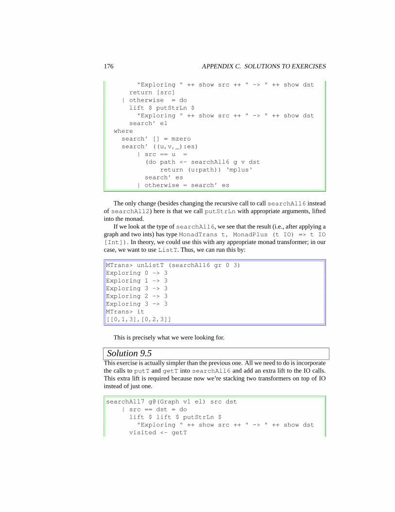
176 APPENDIX C. SOLUTIONS TO EXERCISES
"Exploring " ++ show src ++ " -> " ++ show dstreturn [src]
| otherwise = dolift $ putStrLn $
"Exploring " ++ show src ++ " -> " ++ show dstsearch’ el
wheresearch’ [] = mzerosearch’ ((u,v,_):es)
| src == u =(do path <- searchAll6 g v dst
return (u:path)) ‘mplus‘search’ es
| otherwise = search’ es
The only change (besides changing the recursive call to call searchAll6 insteadof searchAll2) here is that we call putStrLn with appropriate arguments, liftedinto the monad.
If we look at the type of searchAll6, we see that the result (i.e., after applying agraph and two ints) has type MonadTrans t, MonadPlus (t IO) => t IO[Int]). In theory, we could use this with any appropriate monad transformer; in ourcase, we want to use ListT. Thus, we can run this by:
MTrans> unListT (searchAll6 gr 0 3)Exploring 0 -> 3Exploring 1 -> 3Exploring 3 -> 3Exploring 2 -> 3Exploring 3 -> 3MTrans> it[[0,1,3],[0,2,3]]
This is precisely what we were looking for.
Solution 9.5This exercise is actually simpler than the previous one. All we need to do is incorporatethe calls to putT and getT into searchAll6 and add an extra lift to the IO calls.This extra lift is required because now we’re stacking two transformers on top of IOinstead of just one.
searchAll7 g@(Graph vl el) src dst| src == dst = dolift $ lift $ putStrLn $
"Exploring " ++ show src ++ " -> " ++ show dstvisited <- getT

177
putT (src:visited)return [src]
| otherwise = dolift $ lift $ putStrLn $"Exploring " ++ show src ++ " -> " ++ show dst
visited <- getTputT (src:visited)if src ‘elem‘ visitedthen mzeroelse search’ el
wheresearch’ [] = mzerosearch’ ((u,v,_):es)
| src == u =(do path <- searchAll7 g v dst
return (u:path)) ‘mplus‘search’ es
| otherwise = search’ es
The type of this has grown significantly. After applying the graph and two ints, thishas type Monad (t IO), MonadTrans t, MonadPlus (StateT [Int](t IO)) => StateT [Int] (t IO) [Int].
Essentially this means that we’ve got something that’s a state transformer wrappedon top of some other arbitrary transformer (t) which itself sits on top of IO. In ourcase, t is going to be ListT. Thus, we run this beast by saying:
MTrans> unListT (evalStateT (searchAll7 gr4 0 3) [])Exploring 0 -> 3Exploring 1 -> 3Exploring 3 -> 3Exploring 0 -> 3Exploring 2 -> 3Exploring 3 -> 3MTrans> it[[0,1,3],[0,2,3]]
And it works, even on gr4.
Solution 9.6First we write a function spaces which will parse out whitespaces:
spaces :: Parser ()spaces = many (matchChar isSpace) >> return ()
Now, using this, we simply sprinkle calls to spaces through intList to getintListSpace:

178 APPENDIX C. SOLUTIONS TO EXERCISES
intListSpace :: Parser [Int]intListSpace = dochar ’[’spacesintList’ ‘mplus‘ (char ’]’ >> return [])where intList’ = do
i <- intspacesr <- (char ’,’ >> spaces >> intList’)
‘mplus‘(char ’]’ >> return [])
return (i:r)
We can test that this works:
Parsing> runParser intListSpace "[1 ,2 , 4 \n\n ,5\n]"Right ("",[1,2,4,5])Parsing> runParser intListSpace "[1 ,2 , 4 \n\n ,a\n]"Left "expecting char, got ’a’"
Solution 9.7We do this by replacing the state functions with push and pop functions as follows:
parseValueLet2 :: CharParser (FiniteMap Char [Int]) IntparseValueLet2 = choice[ int, do string "let "
c <- letterchar ’=’e <- parseValueLet2string " in "pushBinding c ev <- parseValueLet2popBinding creturn v
, do c <- letterfm <- getStatecase lookupFM fm c ofNothing -> unexpected ("variable " ++
show c ++" unbound")
Just (i:_) -> return i, between (char ’(’) (char ’)’) $ do
e1 <- parseValueLet2

179
op <- oneOf "+*"e2 <- parseValueLet2case op of’+’ -> return (e1 + e2)’*’ -> return (e1 * e2)
]wherepushBinding c v = do
fm <- getStatecase lookupFM fm c ofNothing -> setState (addToFM fm c [v])Just l -> setState (addToFM fm c (v:l))
popBinding c = dofm <- getStatecase lookupFM fm c ofJust [_] -> setState (delFromFM fm c)Just (_:l) -> setState (addToFM fm c l)
The primary difference here is that instead of calling updateState, we use twolocal functions, pushBinding and popBinding. The pushBinding functiontakes a variable name and a value and adds the value onto the head of the list pointed toin the state FiniteMap. The popBinding function looks at the value and if there isonly one element on the stack, it completely removes the stack from the FiniteMap;otherwise it just removes the first element. This means that if something is in theFiniteMap, the stack is never empty.
This enables us to modify only slightly the usage case; this time, we simply takethe top element off the stack when we need to inspect the value of a variable.
We can test that this works:
ParsecI> runParser parseValueLet2 emptyFM "stdin""((let x=2 in 3+4)*x)"
Left "stdin" (line 1, column 20):unexpected variable ’x’ unbound

Index
(), 87∗, 32+, 32++, 38−, 32−−, 52., 50.., 140/, 32//, 144:, 36::, 65==, 65[], 36ˆ, 32ΓE30F , 72λ, 72{−−}, 52, 122
as, 111derive, 134do, 57hiding, 111import, 110qualified, 110
accumArray, 143actions, 95–100arithmetic, 32–34array, 143arrays, 143–145assocs, 144
Bird scripts, 113boolean, 66bounds, 144bracket, 101
brackets, 36buffering, 58
comments, 52–53common sub-expression, 117Compilers, see GHC,NHC,Interpretersconcatenate, 38cons, 36constructors, 81continuation passing style, 87–90CPS, see continuation passing style
destructive update, 31do notation, 173–176do notation, 57drop, 140
Editors, 27–28Emacs, 27
elems, 144Enum, 131–132enumerated types, 84enumFromThenTo, 141enumFromTo, 141Eq, 127–129equality, 65equals, 70evaluation order, 32exceptions, 182exports, 107–110expressions, 32extensions
enablingin GHC, 25in Hugs, 23
fallthrough, 123false, see boolean
180

INDEX 181
files, 42–44filter, 38, 138FiniteMap, 145–147foldl, 38, 139foldr, 38, 138fst, 35functional, 3functions, 44–52
anonymous, see lambdaas arguments, 78–80associative, 40composition, 50type, 71–80
getChar, 101getContents, 101getLine, 58, 101GHC, 19, 23–26guards, 125–127
Haskell 98, 8Haskell Bookshelf, 7hClose, 101head, 37, 74hGetChar, 101hGetContents, 101hGetLin, 101hIsEOF, 101hPutChar, 101hPutStr, 101hPutStrLn, 101Hugs, 19–23
ICFP, 9immutable, 31imports, 110–111indices, 144induction, 54infix, 75, 115–116input, see IOinstance, 67interactive programs, 56–63Interpreters, see GHC,HugsIO, 91–106
library, 100–103isLower, 38
lambda, 72lambda calculus, 72LaTeX scripts, 114layout, 147lazy, 2, 29length, 37, 79let
and do, 175list
comprehensions, 143listArray, 143lists, 35–42, 137–143
comprehensions, 140cons, 36empty, 36
literate style, 112–114local bindings, 117loop, 53
map, 38, 138maps, 145–147Maybe, 85–87modules, 107–114
hierarchical, 111–112monads, 94
and do, 173–176definition of, 170–173laws, 171plus, 181state, 176–181transformer, 181
mutable, see immutable
named fields, 135–137NHC, 19, 26–27null, 74Num, 132numeric types, 70
openFile, 101operator precedence, 33Ord, 130–131output, see IO
pairs, see tuplesparentheses, 33

182 INDEX
pattern matching, 82, 119–125pure, 2putChar, 101putStr, 101putStrLn, 44, 101
random numbers, 59randomRIO, 59Read, 132–133read, 38readFile, 101recursion, 53–56referential tranparency, 31robot, 9
sections, 115–116shadowing, 117Show, 129–130show, 38, 71snd, 35sqrt, 32standard, 8state, 2strict, 2, 152–155strings, 37–38
converting from/to, 38
tail, 37, 74take, 140toUpper, 38true, see booleantuples, 34–35type, 64, 168
checking, 64classes, 69–71, 155–162
instances, 127–134, 162–165datatypes, 80–87, 134–137, 152–
155strict, 152–155
default, 168errors, 66explicit declarations, 77–78hierarchy, 168higher-order, 73–75inference, 64IO, 75–77
kinds, 165–168newtype, 149–152polymorphic, 67–69signatures, 77synonyms, 101, 148–149
Unit, 87unzip, 139user input, see interactive programs
wildcard, 122writeFile, 101
zip, 139