Yanlin Shao1

Odd M. Faltinsen2

1 Ship Hydrodynamics & Stability, Det Norsk Veritas, Norway 2 Centre for Ships and Ocean Structures (CeSOS), NTNU, Norway

1

2

The state-of-the-art potential flow analysis: Boundary Element Method (BEM)

A Cruise Ship A numerical model for BEM

Unknowns distributed on wetted ship surface and water surface

Tune the unknowns so that all boundary conditions and governing equations are satisfied

Still time consuming when it comes to fully-nonlinear problems

2

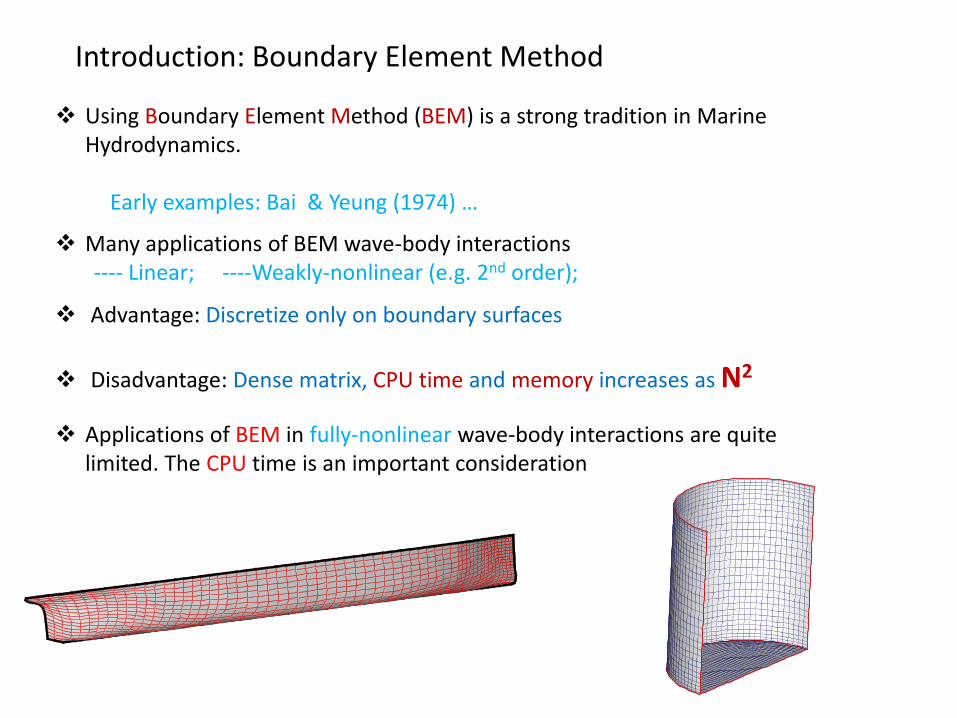
Using Boundary Element Method (BEM) is a strong tradition in Marine Hydrodynamics.

Early examples: Bai & Yeung (1974) …

Introduction: Boundary Element Method

Many applications of BEM wave-body interactions ---- Linear; ----Weakly-nonlinear (e.g. 2nd order); Advantage: Discretize only on boundary surfaces

Disadvantage: Dense matrix, CPU time and memory increases as N2

Applications of BEM in fully-nonlinear wave-body interactions are quite limited. The CPU time is an important consideration

Volume methods are found to be very efficient in terms of CPU time. Advantages to operate with sparse matrix.

Examples: FEM: Wu & Eatock Taylor (1995) , Wang & Wu (2001) FDM: Bingham & Zhang (2007), Engsig-Karup et al. (2009) Advantage: Operate with sparse matrix

Disadvantage: Mesh generation in whole fluid domain

Introduction: Volume Methods

XY

Z

Frame 001 29 Jun 2012 3d contour

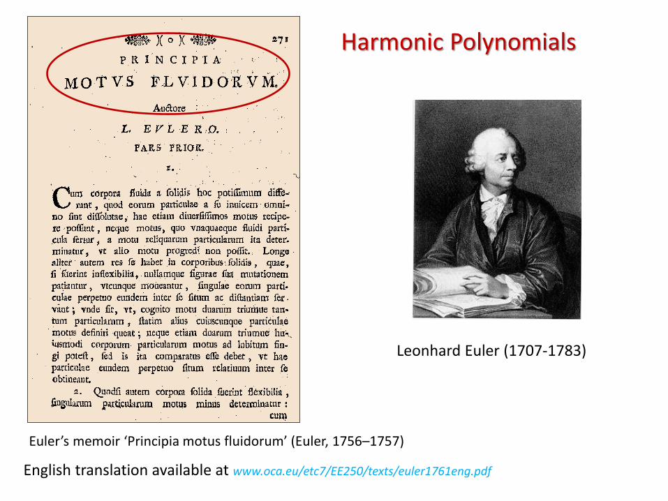
Euler’s memoir ‘Principia motus fluidorum’ (Euler, 1756–1757)

English translation available at www.oca.eu/etc7/EE250/texts/euler1761eng.pdf

Leonhard Euler (1707-1783)

Harmonic Polynomials

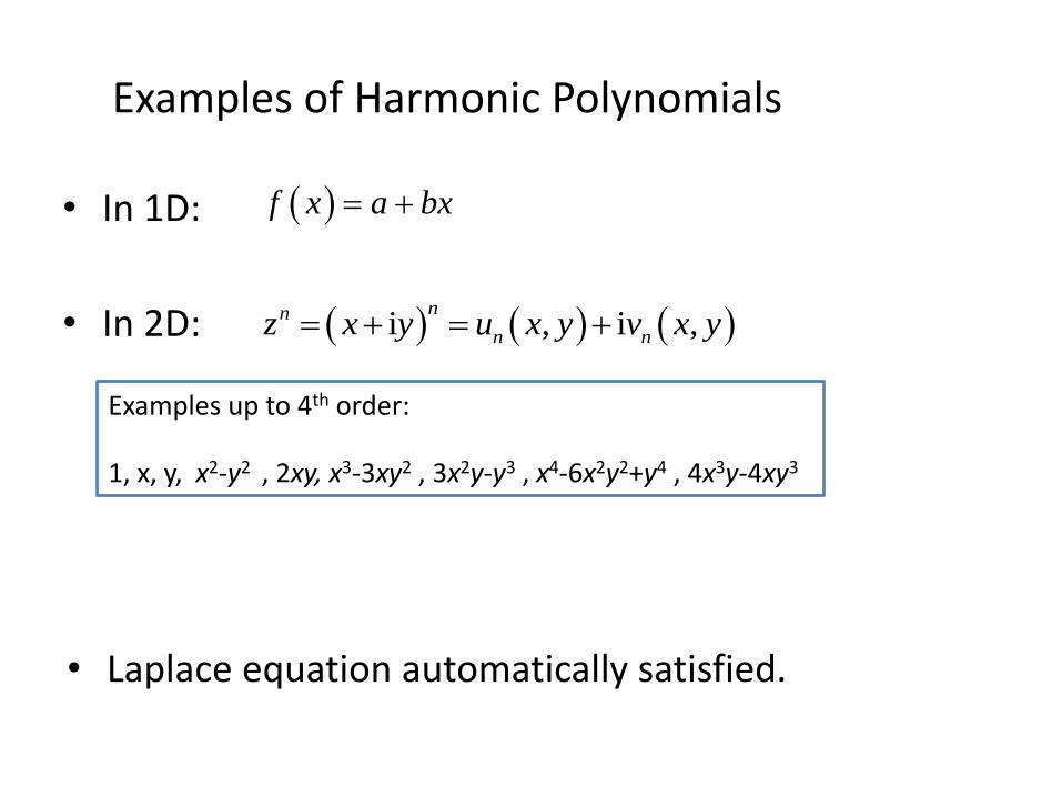
Use polynomials to represent velocity potential Constraints on coefficients in order to satisfy Laplace equation

, ,x y z

2 0

Examples of Harmonic Polynomials

• In 2D: i , i ,nn

n nz x y u x y v x y

Examples up to 4th order:

1, x, y, x2-y2 , 2xy, x3-3xy2 , 3x2y-y3 , x4-6x2y2+y4 , 4x3y-4xy3

• Laplace equation automatically satisfied.

• In 1D: f x a bx

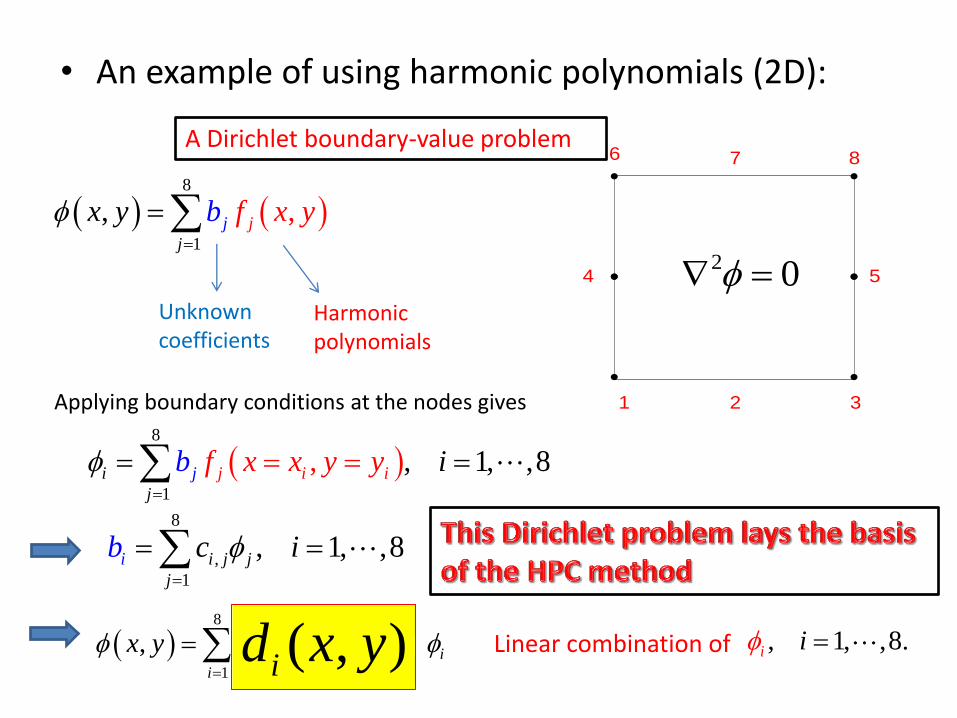
• An example of using harmonic polynomials (2D):

A Dirichlet boundary-value problem

1 2 3

4 5

6 7 8

2 0

8

1

,, j

j

j f x yx by

Unknown coefficients

Harmonic polynomials

Applying boundary conditions at the nodes gives

8

1

, 1,, ,8j ii j

j

if x x y y ib

8

,

1

, 1, ,8i i j j

j

c ib

8 8

,

1 1

, ,j i j i

i j

x y c f x y

Linear combination of , 1, ,8.i i ( , )id x y

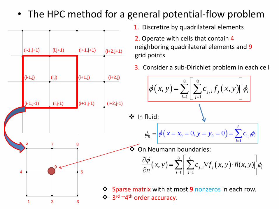
• The HPC method for a general potential-flow problem

(i,j) (i+1,j) (i+2,j)(i-1,j)

(i-1,j-1) (i,j-1) (i+1,j-1) (i+2,j-1)

(i,j+1) (i+1,j+1) (i+2,j+1)(i-1,j+1)

1. Discretize by quadrilateral elements

2. Operate with cells that contain 4 neighboring quadrilateral elements and 9 grid points

1 2 3

4 5

6 7 8

9

3. Consider a sub-Dirichlet problem in each cell

8 8

,

1 1

, ,j i j i

i j

x y c f x y

9

In fluid:

On Neumann boundaries:

8 8

,

1 1

, , ( , )j i j i

i j

x y c f x y n x yn

8

9 9 1,

1

0, 0 i i

i

x x y y c

Sparse matrix with at most 9 nonzeros in each row. 3rd ~4th order accuracy.

Efficiency & Accuracy

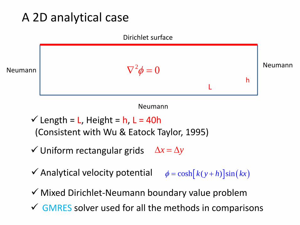
A 2D analytical case

Dirichlet surface

Neumann

2 0 Neumann Neumann

L h

Length = L, Height = h, L = 40h (Consistent with Wu & Eatock Taylor, 1995)

Uniform rectangular grids x y

Analytical velocity potential cosh ( ) sink y h kx

Mixed Dirichlet-Neumann boundary value problem

GMRES solver used for all the methods in comparisons

103

2x103

3x103

0.1

1

10

C

PU

tim

e (

s)

Number of unknowns

BEM

FMM-BEM

FVM

LPC

HPC

103

2x103

3x103

10-8

10-7

10-6

10-5

10-4

10-3

10-2

10-1

100

101

FVM

LPC

HPC

L2 e

rro

rs

Number of unkowns

FMM-BEM, Dirichlet surface

FMM-BEM, Neumann surface

103

2x103

3x103

10-8

10-7

10-6

10-5

10-4

10-3

10-2

10-1

100

101

FVM

LPC

HPC

FMM-BEM, Dirichlet surface

FMM-BEM, Neumann surface

L2 E

rrors

Number of Unknowns

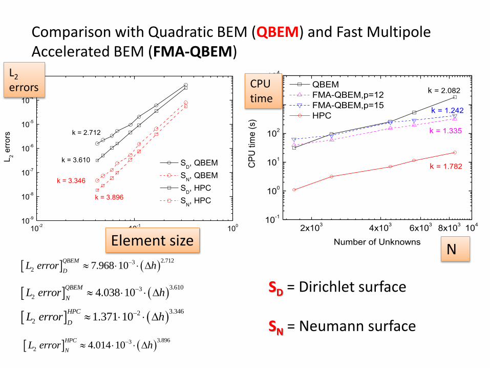
For a given accuracy, HPC performs best

N: number of unknowns corresponding to BEMs

N

CPU time

N N

L2 errors

L2 errors

kh=1.0

kh=6.28

HPC-2D

Required CPU time to achieve 10-4 accuracy

FMM-BEM: > 1 sec

BEM: much much longer time

HPC: 0.06 sec

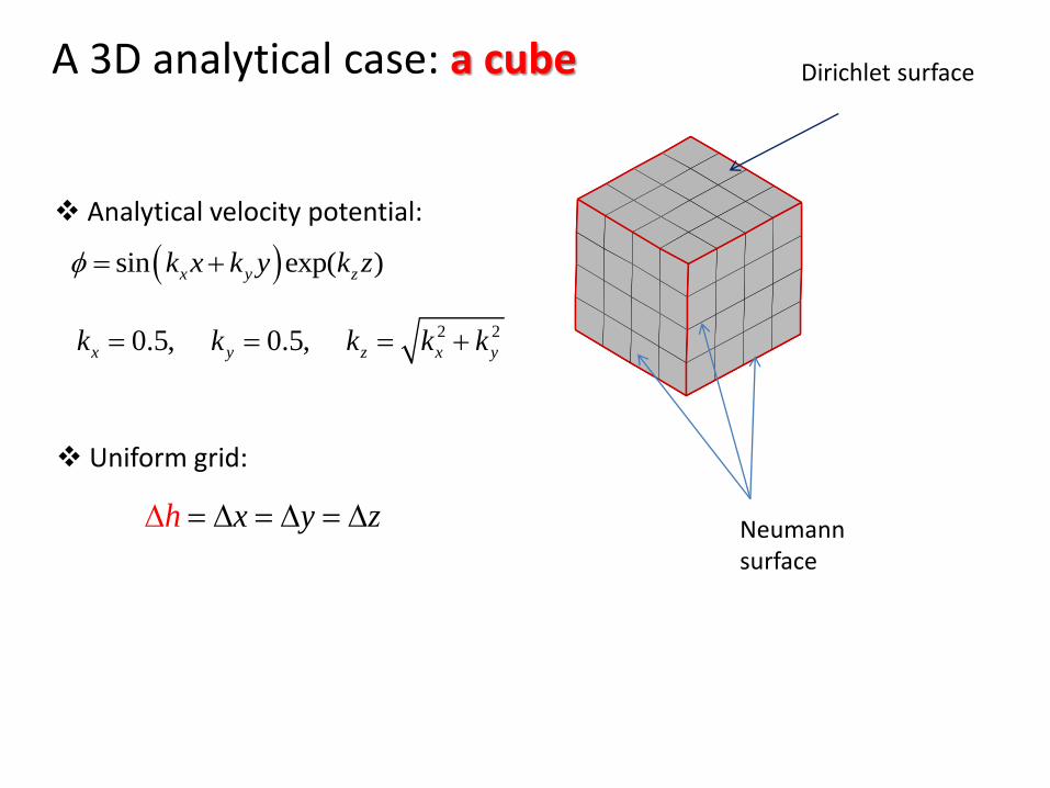
Dirichlet surface

Neumann surface

Analytical velocity potential:

sin exp( )x y zk x k y k z

Uniform grid:

2 20.5, 0.5,x y z x yk k k k k

yh x z

X Y

Z

F ram e 0 0 1 1 7 Apr 2 0 1 2 pane l on episode solid

A 3D analytical case: a cube

10-2

10-1

100

10-9

10-8

10-7

10-6

10-5

10-4

10-3

k = 3.896

k = 3.346

h=2x=2y=2z

L2 e

rro

rs

SD, QBEM

SN, QBEM

SD, HPC

SN, HPC

k = 2.712

k = 3.610

Comparison with Quadratic BEM (QBEM) and Fast Multipole Accelerated BEM (FMA-QBEM)

2x103

4x103

6x103

8x103

104

10-1

100

101

102

103

104

k = 1.782

k = 1.242

k = 1.335

CP

U t

ime

(s)

Number of Unknowns

QBEM

FMA-QBEM,p=12

FMA-QBEM,p=15

HPC

k = 2.082

SD = Dirichlet surface SN = Neumann surface

L2 errors

Element size N

CPU time

2.7123

2 7.968 10QBEM

DL error h

3.6103

2 4.038 10QBEM

NL error h

3.3462

2 1.371 10HPC

DL error h

3.8963

2 4.014 10HPC

NL error h

15

Applications of HPC-2D

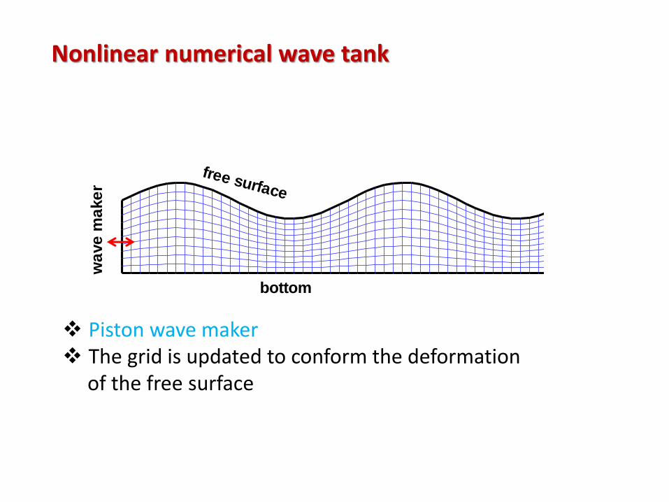
Nonlinear numerical wave tank

free surface

bottom

wa

ve

ma

ke

r

Frame 001 16 Feb 2012 contour lines

Piston wave maker The grid is updated to conform the deformation of the free surface

Trial h (m) e (m) T (s) α β Ur

C 0.4 0.113 3.5 0.105 0.059 30.2

0 5 10 15 20 250.00

0.01

0.02

0.03

0.04

0.05

0.06

1st ,Num,fw=0.025

2nd

,Num,fw=0.025

3rd ,Num,fw=0.025

4th ,Num,fw=0.025

1st ,Num, fw=0.0

2nd

,Num,fw=0.0

3rd ,Num,fw=0.0

4th ,Num,fw=0.0

wave a

mplu

tude (

m)

Distance to wave maker (m)

1st

,exp

2nd

,exp

3rd ,exp

4th ,exp

4

3w

e

hf

A Rayleigh damping term is introduced in the dynamic free surface condition

fw = 0.025 is used

20% of that suggested by Chapalain et al. (1992)

Non-negligible damping effects for higher harmonics

A more rational way of estimating damping effect is needed

20 21 22 23 24 25 26-0.02

-0.01

0.00

0.01

0.02

0.03

0.04

(

m)

t (s)

Num. Exp.

26 27 28 29 30 31 32-0.02

-0.01

0.00

0.01

0.02

0.03

0.04

(

m)

t (s)

Num. Exp.

28 29 30 31 32 33 34-0.02

-0.01

0.00

0.01

0.02

0.03

0.04

t (s)

(

m)

Num. Exp.

35 36 37 38 39 40 41-0.02

-0.01

0.00

0.01

0.02

0.03

0.04

Num. Exp.

t (s)

(

m)

0.4m

0.3m1:

20

1:1

0

6m

6m

2m

3m

13m

12.5m

14.5m

17.3m

21m

Nonlinear waves over submerged trapezoidal bar

Experiments results available from : Beji & Battjes (1993), Luth et al. (1994)

x = 12.5 m x = 14.5 m

x = 17.3 m x = 21 m

19

Applications of HPC-3D

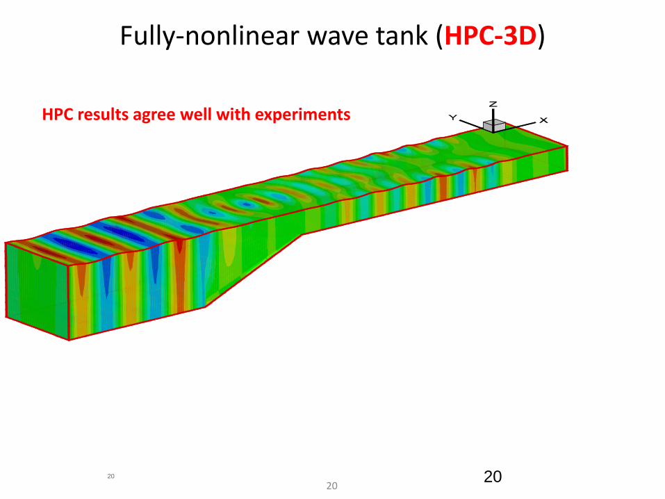
Fully-nonlinear wave tank (HPC-3D)

20 20

XY

ZF ram e 0 0 1 0 2 M ay 2 0 1 2 3 d m eshes | 2 d m esh

Water surface

Sea floor

20

HPC results agree well with experiments

0 5 10 15 20 25 30 350.000

0.004

0.008

0.012

0.016

0.020

0.024

x (m)

wa

ve

am

plit

ud

e (

m)

1st harmonic,exp.

2nd

harmonic,exp.

3rd harmonic,exp.

1st harmonic,num.

2nd

harmonic,num.

3rd harmonic,num.

0 5 10 15 20 25 30 350.000

0.004

0.008

0.012

0.016

wa

ve

am

plit

ud

e (

m)

x (m)

1st harmonic,exp.

2nd

harmonic,exp.

3rd harmonic,exp.

1st harmonic,num.

2nd

harmonic,num.

3rd harmonic,num.

T = 2s; kA = 0.012 T = 2s; kA = 0.017

F ram e 0 0 1 0 9 M ay 2 0 1 2 3 d contour

Fully-nonlinear wave diffraction (HPC-3D)

22 22

Higher order horizontal wave forces in harmonic waves

Comparisons with numerical (Ferrant) and experimental (Huseby&Grue) results

F ra m e 0 0 1 2 2 J a n 2 0 1 3 4 -n o d e s F E M p a n e ls | F E - V o lu m e B ric k D a ta

23

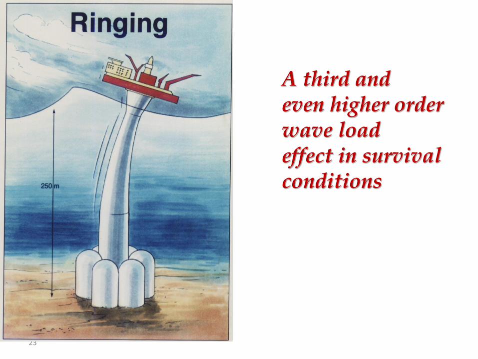
A third and even higher order wave load effect in survival conditions

24

0.00 0.05 0.10 0.15 0.20 0.256.0

6.2

6.4

6.6

6.8

7.0

7.2

kA

Present

Ferrant

|F1| /gA

R2

Analytical

Experiment

2

aF

gAR

0.00 0.05 0.10 0.15 0.20 0.25

0.8

1.2

1.6

2.0

2.4

kA

Arg

(F1)

Analytical

Experiment

Present

Ferrant

arg F

0.00 0.05 0.10 0.15 0.20 0.250.0

0.1

0.2

0.3

0.4

0.5

0.6

0.7

kA

Analytical

Experiment

Present

Ferrant

|F2| /gA

2R

2

2

aF

gA R

0.00 0.05 0.10 0.15 0.20 0.250.0

0.5

1.0

1.5

2.0

2.5

3.0

Arg

(F2)

kA

Present

Ferrant

A

Analytical

Experiment

2arg F

0.00 0.05 0.10 0.15 0.20 0.25-3

-2

-1

0

1

2

3

kA

Arg

(F3)

A

Analytical

Experiment

Present

Ferrant

3arg F

0.00 0.05 0.10 0.15 0.20 0.251

2

3

4

kA

Arg

(F4)

Experiment

Ferrant

Present

A

4arg F

0.00 0.05 0.10 0.15 0.20 0.250.0

0.1

0.2

0.3

0.4

kA

|F3| /gA

3

Present

Ferrant

A

Analytical

Experiment

3

3

aF

gA

0.00 0.05 0.10 0.15 0.20 0.250.0

0.1

0.2

0.3

0.4

0.5

kA

|F

4| /gA

4R

-1 Experiment

Ferrant

Present

4

4 1

aF

gA R

20.245, /g=wave number, radius, wave amplitudekR k R A

25 25

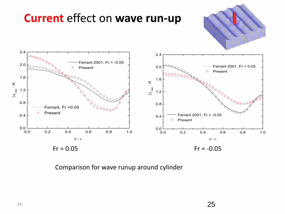
Current effect on wave run-up

0.0 0.2 0.4 0.6 0.8 1.00.0

0.4

0.8

1.2

1.6

2.0

2.4

m

ax

H

Ferrant, Fr =0.05

Present

Ferrant 2001, Fr = -0.05

Present

0.0 0.2 0.4 0.6 0.8 1.00.0

0.4

0.8

1.2

1.6

2.0

2.4

Ferrant 2001, Fr = -0.05

Present

m

ax

H

Ferrant 2001, Fr = 0.05

Present

F ra m e 0 0 1 2 2 J a n 2 0 1 3 4 -n o d e s F E M p a n e ls | F E - V o lu m e B ric k D a ta

Comparison for wave runup around cylinder

Fr = 0.05 Fr = -0.05

Sloshing

0 4 8 12 16 20 24 28-0.08

-0.04

0.00

0.04

0.08

ele

va

tio

n a

t P

1 (

m)

time (s)

HPC

Exp.

Forced oscillation: XT= 0.005L cos(30o), YT= 0.005L sin(30o)

10.90

0 10 20 30 40-0.10

-0.05

0.00

0.05

0.10

ele

va

tio

n a

t P

1 (

m)

time (s)

HPC

Exp.

10.93

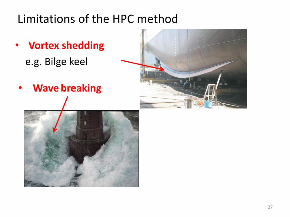
Limitations of the HPC method

• Vortex shedding

e.g. Bilge keel

• Wave breaking

27

A clever strategy: Domain Decomposition

Potential-flow solver

Breaking Fragmentation Air entrainment Viscosity

More advanced solver

Efficiency Accuracy

28

Thank you !

References

• Bai K. J., Yeung R.W., Numerical solutions to free-surface flow problems, Proceedings of 10th Symposium on Naval Hydrodynamics, Cambridge, MA, 1974.

• Wu GX, Eatock Taylor (1995) Time stepping solutions of the two-dimensional nonlinear wave radiation problem. Ocean Engng. 22(8), 785-798.

• Bingham H.B., Zhang H., On the accuracy of finite difference solutions for nonlinear water waves. J. Engineering Math., 58, 211-228, 2007.

• Chapalain G, Cointe R, Temperville A., Observed and modeled resonantly interacting progressive water-waves. Costal Engineering, 16, 267-300, 1992.

• Luth H.R., Klopman G., Kitou N., Kinematics of waves breaking partially on an offshore bar; LDV measurements of waves with and without a net onshore current. Report H-1573, Delft Hydraulics, 1994.

• P. Ferrant, Fully nonlinear interactions of long-crested wave packets with a three dimensional body. In Proceedings of 22nd ONR Symp. in Naval Hydrodynamics, 59-72, 1998.

• A.P. Engsig-Karup, H.B. Bingham, O. Lindberg, An efficient flexible-order model for 3D nonlinear water waves. J. Comput. Phys. 228 (2009) 2100-2118.

• C.H.Wu, O.M. Faltinsen, B.F. Chen, Time-independent finite difference and ghost cell method to study sloshing liquid in 2d and 3d tanks with internal structures. Commun. Comput. Phys. 13 (2013) 780-800.

• Ferrant P., Runup on a cylinder due to waves and current: potential flow solution with fully nonlinear boundary conditions. International Journal of Offshore and Polar Engineering. 11(1), 2001.

• Euler L., Principles of the motion of fluids, Physica D: Nonlinear Phenomena 237 (2008) 1840-1854.

• Shao Y.L., Faltinsen O.M., Towards efficient fully-nonlinear potential-flow solvers in marine hydrodynamics. in: Proc. of the 31st Int. Conf. on Ocean, Offshore and Arc. Eng. (OMAE). Rio de Janeiro, Brazil, 2012.

• Shao Y.L., Faltinsen O.M., A Harmonic polynomial cell (HPC) method for 3D Laplace equation with application in marine hydrodynamics. Submitted for journal publication.

• Shao Y.L., Faltinsen O.M., Use of body-fixed coordinate system in analysis of weakly-nonlinear wave-body problems. Appl. Ocean Res., 32, 1, 20-33, 2010.