Alvin M. Despain

Domenico Ferrari

Finbarr O’Sullivan

Yale N. Patt

Performance Enhancement ThroughDynamic Scheduling and Large Execution-Atomic-Units in

Single Instruction Stream Processors

by

Stephen Melvin

Abstract

This dissertation demonstrates that through the careful application of hardware and software

techniques, general purpose code can be executed more than twice as fast as previously thought

possible. Exploiting parallelism is critical to high performance. The type of parallelism focused on

in this dissertation is intra-instruction stream, or fine-grained, parallelism. This is the parallelism

available within a small dynamic window of instructions executed on a single instruction stream

processor. Three mechanisms are analyzed on realistic processors running general purpose code and

it is shown that a higher degree of fine-grained parallelism can be exploited than has previously been

achieved.

It has been suggested that general purpose, or non-scientific, programs have very little parallelism

not already exploited by existing processors and can achieve a speedup of at most approximately

two. The argument is made that there is little to be gained by complex processor control logic; simple

issuing and scheduling mechanisms are sufficient to exploit all the parallelism available. This idea

has impeded the development of multiple function unit processors. In this dissertation it is shown

that, contrary to this notion, there is actually a significant amount of unexploited parallelism in typical

general purpose programs.

Three performance enhancement techniques are analyzed: dynamic scheduling, dynamic branch

prediction and basic block enlargement. Dynamic scheduling involves the decoupling of operations

1

within a single instruction word, allowing them to be scheduled independently. Dynamic branch

prediction involves the use of speculative execution. Basic block enlargement is a technique that

relies on compile time effort and an efficient backup mechanism to exploit parallelism more

effectively. It is shown that indeed for narrow instruction words little is to be gained by the application

of these three techniques. However, as the number of function units increases, it is possible to achieve

speedups of almost five on realistic processors.

Yale N. Patt Dissertation Committee Chair

2

Acknowledgements

This dissertation has grown out of a group project at Berkeley known as HPS (High Performance

Substrate) and has benefited from the contributions of many individuals. Foremost among them is

Yale Patt, the originator of the HPS project and an unequaled research advisor. Through combined

patience and encouragement, he has allowed me to follow my own direction but provided careful

guidance when needed. In addition, his vast experience and depth of knowledge have proved to be

invaluable.

My colleagues on the HPS project also deserve mention, in particular Michael Shebanow and

Wen-mei Hwu. Our interaction in the early days of HPS was rewarding and educational. Later,

Wen-mei provided many insights in the course of his dissertation research and Mike contributed to

many ideas that are part of the abstract machine model I developed. Others in the HPS project were

beneficial as well, including Chien Chen, Allen (Jiajuin) Wei, Ashok Singhal, Jeff Gee and Jim

Wilson.

HPS was part of a larger project at Berkeley known as Aquarius, led by Alvin Despain. He

provided much valuable input and his vision and leadership allowed the overall atmosphere in the

group to be supportive and stimulating. There were many others within the Aquarius group that also

contributed. In addition, many within the Computer Science Division were instrumental in shaping

this dissertation into its present form, in particular Domenico Ferrari who provided many useful

comments.

Finally, I’d like to make a special acknowledgement of William Kahan. Of all the professors I

have known in my ten years at Berkeley, he has demonstrated the most genuine concern for students.

His assistance during the final phase of this dissertation, his encouragement and his help with

administrative matters was beyond comparison.

ii

Table of Contents

Chapter 1 Introduction.............................................................................................................. 1

Chapter 2 Historical Background ............................................................................................ 6

2.1 Single Instruction Stream Processors............................................................................ 6

2.1.1 Concurrency Handling Mechanisms ..................................................................... 6

2.1.2 Historical Summary ................................................................................................ 8

2.2 Previous Parallelism Studies ........................................................................................ 10

2.2.1 Measurement Limitations ..................................................................................... 10

2.2.1.1 Conditional Branches ..................................................................................... 11

2.2.1.2 Compiler/Architecture Artifacts................................................................... 11

2.2.1.3 Processor/Memory Limitations..................................................................... 13

2.2.2 Summary of Previous Studies ............................................................................... 14

Chapter 3 Models of Execution .............................................................................................. 24

3.1 The Interface Model ...................................................................................................... 24

3.1.1 Definitions ............................................................................................................... 25

3.1.2 Historical Background........................................................................................... 28

3.1.3 DSI Tradeoffs ......................................................................................................... 29

3.1.4 DSI Placement Examples ...................................................................................... 31

3.2 The Atomic Unit Model................................................................................................. 36

3.2.1 Definitions ............................................................................................................... 37

3.2.2 Atomic Unit Tradeoffs ........................................................................................... 38

3.2.3 CAU and EAU Size Examples .............................................................................. 39

Chapter 4 Microarchitectural Mechanisms.......................................................................... 42

4.1 Local Parallelism ........................................................................................................... 42

4.2 Dynamic Scheduling ...................................................................................................... 44

4.3 Dynamic Branch Prediction ......................................................................................... 49

iii

4.4 Basic Block Enlargement.............................................................................................. 51

4.5 Dynamic Scheduling / Basic Block Enlargement Tradeoffs ..................................... 55

Chapter 5 The Abstract Processor Model............................................................................. 58

5.1 Model Overview............................................................................................................. 59

5.2 Instruction unit .............................................................................................................. 64

5.2.1 Fill Unit.................................................................................................................... 65

5.2.2 Basic Block Sequencer ........................................................................................... 69

5.3 Scheduling Unit.............................................................................................................. 72

5.3.1 Register Alias Tables ............................................................................................. 72

5.3.2 Node Tables............................................................................................................. 74

5.3.3 Memory Node Tables............................................................................................. 76

5.4 Execution Unit................................................................................................................ 79

5.5 Memory Unit .................................................................................................................. 80

Chapter 6 Simulation Description and Results..................................................................... 84

6.1 Simulator Overview....................................................................................................... 84

6.1.1 Translating Loader ................................................................................................ 86

6.1.1.1 Node Generator............................................................................................... 88

6.1.1.2 Fill Unit ............................................................................................................ 91

6.1.2 Run-time Simulator ............................................................................................... 93

6.2 Experimental Methodology .......................................................................................... 97

6.2.1 Experimental Parameters ..................................................................................... 97

6.2.2 Data Collection Procedures................................................................................... 99

6.3 Simulation Results and Analysis ................................................................................ 102

Chapter 7 Conclusions........................................................................................................... 118

7.1 Limits of Single I-Stream Processors ........................................................................ 119

7.1.1 Architectural Considerations.............................................................................. 121

iv

7.1.2 Compiler Techniques ........................................................................................... 124

7.2 Areas of Future Research ........................................................................................... 126

7.2.1 Multiple Instruction Stream Processors............................................................ 126

7.2.2 Adaptive Basic Block Enlargement.................................................................... 128

References..................................................................................................................................... 130

Appendix A Node Opcodes........................................................................................................ 142

Appendix B Benchmark Input and Output ............................................................................. 146

v

Chapter 1 Introduction

This dissertation focuses on several different hardware and software techniques to speed up single

instruction stream processors. Enhancements to computer performance can be broadly placed into

two main categories: technological and architectural. Technological advances involve finding new

materials and techniques to make gates that switch faster and memories that can be accessed faster.

Architectural advances involve restructuring these gates and memories to allow more operations to

occur at the same time (i.e. achieving some degree of parallelism). Technological advances have

dominated increases in speed in the past but the technology is approaching fundamental limits. Future

increases in performance will be forced to rely more heavily on advances in computer architecture,

allowing more parallelism to be exploited.

Architectural advances involve changes in software as well as hardware. In order to exploit higher

degrees of parallelism, changes are required at all levels of an overall computer system. One basic

distinction is that between exploiting parallelism across instruction streams (inter-instruction stream

parallelism) and exploiting parallelism within a single instruction stream (intra-instruction stream

parallelism). When we speak of an instruction stream, we mean a set of instructions, formatted in

any manner, with a definite sequencing implied. That is, we assume that the instruction stream

presents a sequential control model. Between control points there may not necessarily be a particular

sequence of operations, but we assume that there is a single specified sequence of control points.

Consider the design of a multiprocessor computer system. An important question is how to

partition a fixed hardware cost for maximum performance. Is it better to supply a larger number of

simpler processors or a smaller number of more complex processors? There are not simply two

alternatives involved but a continuous spectrum of design choices. Even designs that lean heavily

on the side of complex processors can benefit from techniques for partitioning a job into multiple

instruction streams. Conversely, designs that lean toward lots of small processors can benefit from

techniques to get more speedup within an instruction stream.

1

The critical parameter for this spectrum of design choices is the hardware cost per instruction

stream. In some situations it makes sense to spend very little hardware per instruction stream, and

in others it makes sense to spend as much as possible. A low hardware cost per instruction stream

stresses inter-instruction stream parallelism while a high cost stresses intra-instruction stream

parallelism. The main issues are the availability of each type of parallelism and at what expense in

discovery. Some of the main design issues are the following:

• Ease of design and manufacture; time to market

• Chip boundaries

• Application space

Simple processors have the advantage of being easy to design and build. This makes them

inexpensive and able to exploit new technology sooner. A more complex processor which can

execute a single instruction stream faster than a simple one may not pay for itself in many applications.

Also, there may be chip boundary effects to consider. That is, if in a particular implementation the

ratio between on-chip speed to off-chip speed is significant, it will tend to be more cost effective to

use processors that are simple enough to fit on a single chip.

Having a larger number of simple processors has the problem of requiring more independent

instruction streams. In some applications, for example the multitasking support of a large user base,

finding independent instruction streams is not difficult. In other applications, it may be necessary to

solve a single problem on such a system. The burden of partitioning a large problem such as this

into multiple instruction streams can fall on the compiler, on the assembly language programmer

and/or on the application programmer. In some applications, it may be difficult or impossible to

create a large number of instruction streams. Another consideration is that communication is

increased in a system with many processors and this may result in lower efficiency due to

synchronization.

In many applications, for example matrix multiply, the parallelism is so explicit that uncovering

it is trivial. For these types of applications, the processor design is almost irrelevant. Unless there

2

is a significant imbalance between the number of registers and the ratio of computation to memory

speed, it should be possible to get close to 100% utilization of function units. Therefore, other factors

become more important, for example how the memory and processors are interconnected. In this

dissertation we are concerned with non-scientific, or general purpose code which does not have this

property that discovering parallelism is trivial. The main properties of general purpose code as

opposed to scientific code are:

• Basic blocks are smaller (i.e. a fewer number of operations between control points)

• Branches are hard to predict statically

• Memory access patterns are hard to determine statically

We will show that it is possible to exploit parallelism from non-scientific code, but doing so has a

higher cost in hardware and in software than that for scientific code.

We have been implicitly assuming in this discussion that all processors are identical and each

executes only one instruction stream. An alternative would be a heterogeneous multiprocessor with

some simple processors and some complex processors. This would allow applications at different

ends of the spectrum to take advantage of the parts of the machine most appropriate to them. Another

possibility would be processors that can execute more than one instruction stream simultaneously.

This would allow the system to dynamically move on the spectrum, optimizing for the current

operating conditions (we discuss this type of machine further in chapter 7).

One could argue that the maximum performance achievable for an instruction stream occurs at a

point of fairly low cost. The notion is that increasing the complexity of the processor will

categorically slow the processing down to the point that it will always negate any performance gain.

If this were the case then regardless of other factors, the optimal computer system would always have

simple processors. We reject this notion for two reasons. First, as we will show later, there exists a

significant amount of parallelism in most instruction streams that is not exploited by most processors.

Second, this notion contradicts historical trends in processor design.

3

For a given technology, processors have continually increased in complexity (and in performance).

Processors have not always increased in complexity when compared across technologies and when

‘social’ reasons are considered (i.e. marketing, object code compatibility, etc.). However, as a

particular technology matures and allows a greater degree of complexity to be managed, it has

invariably been advantageous to do so.

Several recent studies, for example [JoWa89] and [SmLH90], have suggested that most general

purpose instruction streams have very little parallelism available, allowing a speedup on the order

of at most about two. This has caused some to say that intra-instruction stream parallelism is at its

limit and that future increases in performance must rely solely on inter-instruction stream parallelism.

We will explain in chapter 2 why these studies do not apply here. We will show in this dissertation

that the limits of single instruction stream performance are far from being reached in existing

processors. This dissertation focuses on this issue: examining architectural techniques to allow faster

execution of single instruction streams. Note that even designs geared to simple processors may

benefit from techniques to increase intra-instruction stream parallelism if the increase in performance

is great enough and the additional cost small enough. The purpose of this dissertation is to explore

that increase in performance and that additional complexity.

Statement of the Thesis

Contrary to conventional wisdom, which states that non-scientific instruction streamscontain negligible amounts of unexploited parallelism, a significant amount of easilydetectable parallelism actually exists in most general purpose instruction streams that isnot exploited by existing processors. Much of this untapped parallelism can be releasedby dynamically scheduling nodes onto function units, as opposed to scheduling themstatically, and by increasing the sizes of the execution-atomic-units.

This dissertation has seven chapters. Chapter 2 provides historical background at two levels. First,

we discuss the history of architectural improvements to single instruction stream processors. We

classify processors as to how they have handled data dependencies, resource conflicts and branches.

Then we look at previous studies of single instruction stream parallelism. There have been many

studies measuring available fine grained parallelism with widely varying results. We discuss some

of the most significant ones and comment on their limitations.

4

Chapter 3 presents two models of execution that provide a framework for the remaining chapters.

We discuss the interface model and the atomic unit model. The interface model is mainly concerned

with two interfaces: the hardware/software interface and the dynamic/static interface, and with

distinctions between the two. The atomic unit model is concerned with the manner in which nodes

are combined into atomic units. We define compiler atomic units, execution atomic units and

architectural atomic units.

In chapter 4 we present three microarchitectural mechanisms: dynamic scheduling, dynamic

branch prediction and basic block enlargement. These three closely related mechanisms are the focus

of the performance enhancement techniques analyzed in this dissertation. Dynamic scheduling

involves the decoupling of individual operations from others in the instruction stream so that they

may be executed more or less independently. Dynamic branch prediction, as it is defined here,

involves the use of speculative execution to exploit parallelism across branches. Basic block

enlargement is a technique used in conjunction with some sort of backup logic to increase the effective

size of the basic blocks being executed.

Chapter 5 introduces the abstract processor model. This is a model of a single instruction stream

processor incorporating features needed for analyzing the mechanisms of chapter 4. Aspects which

are not relevant to the issues being addressed are left unspecified and aspects that are directly

addressed are parameterized by the model. The abstract processor model of chapter 5 is used as the

basis for the simulation study, which is described in chapter 6. We outline the simulation process,

present the experimental methodology, and report on the results of the study. Finally, chapter 7

concludes with discussions on other aspects which limit single instruction stream performance and

areas of future research.

5

Chapter 2 Historical Background

In this chapter we present historical background at two different levels. In the first section we

discuss single instruction stream processors in general. We look at the history of how simultaneous

execution of operations has been applied to exploit fine-grained parallelism. In the second section

we look at previous studies of the parallelism available in single instruction streams. We summarize

a number of such studies and discuss their limitations.

2.1 Single Instruction Stream Processors

In this section we provide a brief historical overview of concurrency in the data paths of single

instruction stream machines. We first categorize concurrency handling mechanisms within a

processor. Then we trace historical developments in how different mechanisms have been applied.

We are only concerned here with data path concurrency, that is the arithmetic units (ALUs) and

paths to memory. We will not consider issues relating to the format of the instruction stream; how

it is fetched or how it is decoded. These are important issues in their own right, but they are not the

focus of this dissertation.

2.1.1 Concurrency Handling Mechanisms

Concurrency can be broadly categorized into two areas: pipelining and parallelism. Pipelining

involves allowing a single arithmetic unit or path to memory to accept new inputs before it has

completely generated the result of previous inputs. Parallelism involves the use of multiple arithmetic

units or paths to memory. When we mention simultaneous or overlapped or concurrent operations,

we mean operations which are executed with some degree of pipelining and/or parallelism. A

processor in which operations are executed singly and each operation is fully executed before the

next begins would be a completely non-concurrent design.

Whenever concurrency is exploited in single instruction stream processors, three issues become

important: how to resolve data dependencies, how to resolve resource conflicts (if they are possible),

6

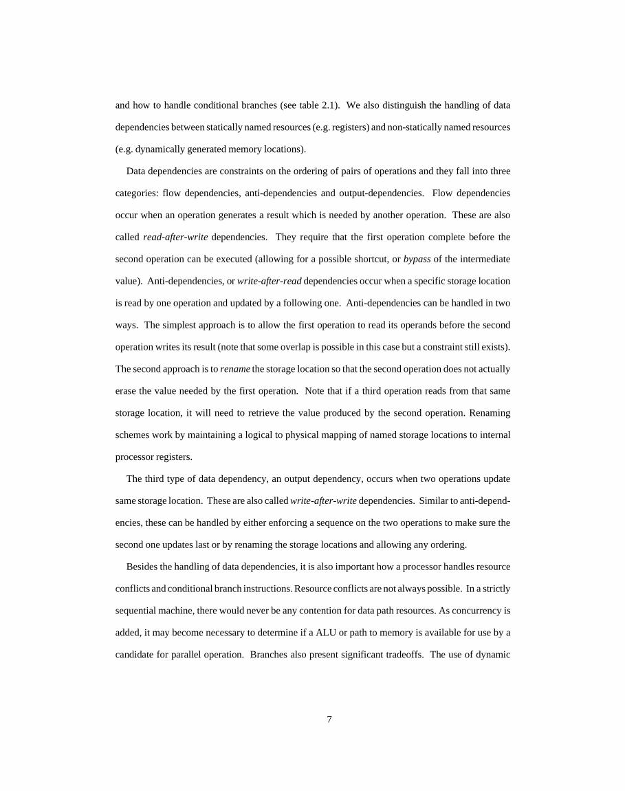
and how to handle conditional branches (see table 2.1). We also distinguish the handling of data

dependencies between statically named resources (e.g. registers) and non-statically named resources

(e.g. dynamically generated memory locations).

Data dependencies are constraints on the ordering of pairs of operations and they fall into three

categories: flow dependencies, anti-dependencies and output-dependencies. Flow dependencies

occur when an operation generates a result which is needed by another operation. These are also

called read-after-write dependencies. They require that the first operation complete before the

second operation can be executed (allowing for a possible shortcut, or bypass of the intermediate

value). Anti-dependencies, or write-after-read dependencies occur when a specific storage location

is read by one operation and updated by a following one. Anti-dependencies can be handled in two

ways. The simplest approach is to allow the first operation to read its operands before the second

operation writes its result (note that some overlap is possible in this case but a constraint still exists).

The second approach is to rename the storage location so that the second operation does not actually

erase the value needed by the first operation. Note that if a third operation reads from that same

storage location, it will need to retrieve the value produced by the second operation. Renaming

schemes work by maintaining a logical to physical mapping of named storage locations to internal

processor registers.

The third type of data dependency, an output dependency, occurs when two operations update

same storage location. These are also called write-after-write dependencies. Similar to anti-depend-

encies, these can be handled by either enforcing a sequence on the two operations to make sure the

second one updates last or by renaming the storage locations and allowing any ordering.

Besides the handling of data dependencies, it is also important how a processor handles resource

conflicts and conditional branch instructions. Resource conflicts are not always possible. In a strictly

sequential machine, there would never be any contention for data path resources. As concurrency is

added, it may become necessary to determine if a ALU or path to memory is available for use by a

candidate for parallel operation. Branches also present significant tradeoffs. The use of dynamic

7

branch prediction (see chapter 4) allows operations to be executed before the direction of the branch

preceding them has been resolved. We will show below that there are many options to addressing

each of these three issues. Often there are tradeoffs associated with how much of these functions is

handled in hardware and how much is handled in software.

2.1.2 Historical Summary

Early processors had no data path concurrency. There was no pipelining of operations and no

parallel use. The UNIVAC I was one of the first machines to employ concurrency by overlapping

program execution with I/O operations. Concurrency within the processor started with the pipelining

of instruction fetches. The IBM 7094 had a 72-bit wide memory and 36-bit instructions, so half the

instruction fetches could be eliminated in sequential code. The next step was the pipelining of data

memory accesses through the use of interleaved memory, employed in the IBM 7094 II.

As a natural extension of memory pipelining and instruction pre-fetching, machine designers

started to pipeline the execution phase. The Stretch and the LARC were two of the first processors

to employ execution pipelines. The Stretch had a two stage pipeline: instruction fetch and decode

and data execution while the LARC had a four stage pipeline: instruction fetch, address index

operations, data fetch and data execution. In these machines the issue of data dependencies started

Table 2.1Summary of Single Instruction Stream Concurrency

Concept,Machine

Data DependenciesResource Conflicts

BranchHandlingStatic

AddressNon-static Address

Early Processors no overlap no overlap not possible no overlap

Execution Pipelines pipeline stall sequential not possible wait

CDC 6600 / 7600 scoreboard sequential scoreboard wait

IBM 360/91 tag forward dynamic test tag forward wait

Vectors compiler sequential scoreboard wait

VLIW compiler sequential compiler no interlock

Decoupled tag forward dynamic test tag forward dynamic

8

to become important. These early pipelined processors employed a simple dependency preservation

scheme in which an operation requiring a result not yet generated simply waited and held up

everything behind it.

Processors were then developed with multiple function units. The CDC6600 had a register

scoreboard which kept track of register reads and writes in order to detect dependencies. In the

absence of dependencies and as long as the appropriate function unit was not busy, instructions could

continue to be issued. In the CDC7600, pipelining was added to the function units, permitting even

more concurrency. A disadvantage of the register scoreboard scheme is that, when an instruction

blocks due to a resource or dependency conflict, it holds up all subsequent instructions. Another

disadvantage is that anti-dependencies and output dependencies hold up execution even though they

are only artifacts of a limited number of registers.

A mechanism that gets around these two disadvantages is the tag-forwarding scheme of Tomasulo

employed on the IBM 360/91. In this scheme operations wait in ‘reservation stations’ until their

operands are ready, allowing following instructions to continue. Also, anti-dependencies and output

dependencies are removed by separating the logical registers (architectural) from the physical ones

(reservation station locations).

Extending the concept of execution pipelines, vector operations allow the compiler to organize an

entire set of operations with explicitly known dependencies. These groups of data, or vectors, can

be pipelined very efficiently with appropriate hardware. In some applications, it is relatively easy

for the compiler to find many such operations. The Cray I employed vector operations as well as a

register scoreboard to take advantage of the explicit dependencies of vectors with multiple function

units.

VLIW machines are analogous to vector operations in that they allow the compiler to explicitly

label dependencies, but for parallelism rather than pipelining. Multiple operations are dispatched in

each cycle, having been organized into groups by the compiler. These machines typically have very

little hardware dependency detection, putting the job mostly on the compiler to avoid conflicts. The

9

Multiflow Trace is one such commercial product. Using advanced compiler techniques, known as

‘trace scheduling,’ operations across many branches can be used to fill slots in instruction words.

Statically scheduled machines machines such as these tend to work best on code with branches

that are easy to predict statically, for example loops with known numbers of iterations. Another

constraint to static scheduling is variability in memory latency, requiring pipelines to stall to satisfy

memory requests longer than the compiler predicted. Dynamically scheduled, or decoupled proces-

sors get around these problems by having the hardware detect and satisfy all or most of the

dependencies. The concept of tag forwarding is extended in these machines to cover both memory

and ALU operations. Also, memory disambiguation, which is the comparison of memory addresses

to detect dependencies, takes place dynamically. Dynamic branch prediction is also generally used

to allow concurrency to be exploited across branches.

2.2 Previous Parallelism Studies

In the previous section we addressed how fine-grained, or instruction-level, parallelism is

exploited. In the section we will deal with a more fundamental issue: how much is actually available

to be exploited? Many studies have been performed which indicate that the maximum is less than

two. One effect of these studies has been the inhibition of the development of software and hardware

mechanisms for exploiting single instruction-stream parallelism.

However, the issue remains unresolved. One reason for this is that analyzing fine-grained

parallelism is intimately connected with specific execution models. As we will show, most studies

are closely tied to specific compiler, architectural and microarchitectural mechanisms. In this section

we look at the validity of generalizing these results. We will explore the relevance of several previous

studies to the application of new software and hardware techniques for exploiting parallelism in

single instruction streams.

2.2.1 Measurement Limitations

In this section we will discuss several different limitations that are common in measurements of

10

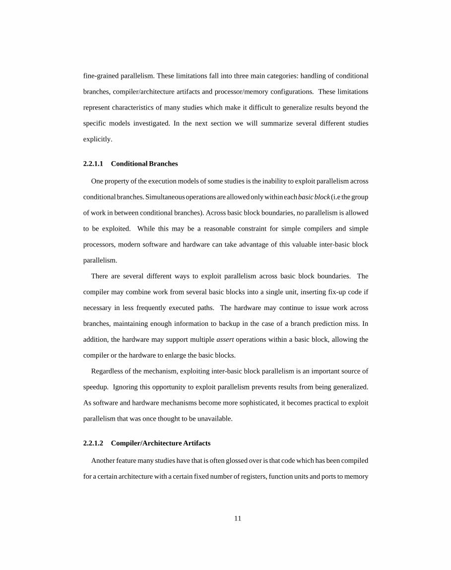
fine-grained parallelism. These limitations fall into three main categories: handling of conditional

branches, compiler/architecture artifacts and processor/memory configurations. These limitations

represent characteristics of many studies which make it difficult to generalize results beyond the

specific models investigated. In the next section we will summarize several different studies

explicitly.

2.2.1.1 Conditional Branches

One property of the execution models of some studies is the inability to exploit parallelism across

conditional branches. Simultaneous operations are allowed only within each basic block (i.e the group

of work in between conditional branches). Across basic block boundaries, no parallelism is allowed

to be exploited. While this may be a reasonable constraint for simple compilers and simple

processors, modern software and hardware can take advantage of this valuable inter-basic block

parallelism.

There are several different ways to exploit parallelism across basic block boundaries. The

compiler may combine work from several basic blocks into a single unit, inserting fix-up code if

necessary in less frequently executed paths. The hardware may continue to issue work across

branches, maintaining enough information to backup in the case of a branch prediction miss. In

addition, the hardware may support multiple assert operations within a basic block, allowing the

compiler or the hardware to enlarge the basic blocks.

Regardless of the mechanism, exploiting inter-basic block parallelism is an important source of

speedup. Ignoring this opportunity to exploit parallelism prevents results from being generalized.

As software and hardware mechanisms become more sophisticated, it becomes practical to exploit

parallelism that was once thought to be unavailable.

2.2.1.2 Compiler/Architecture Artifacts

Another feature many studies have that is often glossed over is that code which has been compiled

for a certain architecture with a certain fixed number of registers, function units and ports to memory

11

is often used to simulate a processor with a different configuration. The exact influence of this feature

is hard to gauge. The degree to which the compiler optimizes for the architecture as well as the

relationship between the compiled-to architecture and the simulated architecture are involved.

One common technique is to add register renaming as a final step to code that has already been

compiled for a small number of registers. The idea is to remove false dependencies between registers

so that the true parallelism can be examined. The problem is that this technique will only partially

remove artifacts of the architecture. The ability of the compiler to optimize (e.g. eliminate common

sub-expressions and redundant memory accesses) is influenced by how many registers are available.

Register renaming will not eliminate additional nodes or propagate literals to unchain flow depend-

a = *++p;b = *++p;

+

+

READ

+

READREAD

+

READ

a

4

p

p

p

44 8

q

Figure 2.1Compiler/Architecture Optimization Example

p

a b

b

q <-- p + 4 a <-- mem[q] p <-- p + 8 b <-- mem[p]

p <-- p + 4 a <-- mem[p] p <-- p + 4 b <-- mem[p]

p

12

encies.

Consider the example shown in figure 2.1. Suppose we have a simple pair of C statements that

read two adjacent 32-bit quantities as shown. A straightforward way to compile this code would be

as shown on the left (we assume a, b, p and q are general purpose registers). The p variable is

incremented twice. In a processor with a single ALU, there would be no advantage to the compiler

to save the first address in a register different from p and have the second address computation add

8 instead of 4, as shown on the right. In fact there would be a disadvantage because it requires the

additional register q.

Now, suppose we take this sequential code and simulate a processor with infinite resources. In

the first case, three steps are required while in the second case only two are needed. It is the alternate

sequence on the right which would be more optimal given that the two adds can take place

simultaneously. Register renaming will not discover artificial flow dependencies like this. It is only

by having the compiler or the hardware re-optimize an entire group of work that these effects can be

removed.

However, this should not be interpreted as meaning that register renaming, or its more general

form tag forwarding is not useful for new architectures. Even if a compiler is designed for a specific

hardware configuration, these techniques are important in consideration of conditional branches,

variability in memory latency and dynamic memory disambiguation. We discuss this further in

chapter 4. In any case, it should be clear that results which use code compiled for specific

implementations are hard to generalize to other processors.

2.2.1.3 Processor/Memory Limitations

The third main area in which studies of fine-grained parallelism are often limited has to do with

the interface between the processor and memory. Frequently only a single memory operation per

cycle is allowed. While this may be a reasonable constraint for simple processors, results collected

this way tell us very little about how much parallelism is available to processors with wider paths to

memory.

13

Another common feature is the lack of dynamic memory disambiguation. If a compiler is forced

to decide statically which memory operations are dependent, it must make conservative assumptions

about dynamically generated memory addresses. Thus, speedup measurements made under these

circumstances may not represent the total speedup available to a processor which disambiguates

memory addresses run-time, potentially overlapping more memory operations.

Finally, often memory is modeled as a perfect cache. The introduction of variability into memory

latency changes tradeoffs associated with operation scheduling. Unlike the other limitations we have

been discussing, this will make results more optimistic instead of more pessimistic. However, it will

change the performance of different mechanisms, clouding relative comparisons.

2.2.2 Summary of Previous Studies

Table 2.2 summarizes ten previous studies that have been made on the degree of available

instruction level parallelism. It should be mentioned that many of these studies have focused on

other issues. We will discuss only those aspects of the studies that are related to fine-grained

parallelism; thus, it should not be inferred from this section that the studies did not have other

significant features.

In the earliest study [TjFl70], Tjaden and Flynn analyze the speedup achievable by allowing

multiple instructions to issue simultaneously. They analyzed a modified IBM 7094 in which adjacent

sequences of instructions could be executed simultaneously if no dependencies existed. They

allowed an unlimited number of additional registers to be used in order to eliminate anti and output

dependencies, but they did not increase the number of function units. They concluded that an average

of between 1.2 and 3.2 independent instructions could be found per cycle by implementing

pre-decode stack which looked ahead 10 instructions.

The main limitation of this study is that the function unit configuration was the same as the 7094.

No additional function units or ports to memory were simulated. Thus, we do not know how much

performance improvement is limited by flow dependencies and how much is limited by resource

conflicts. Also, the instruction stream was not altered from 7094 compiled code. Even though an

14

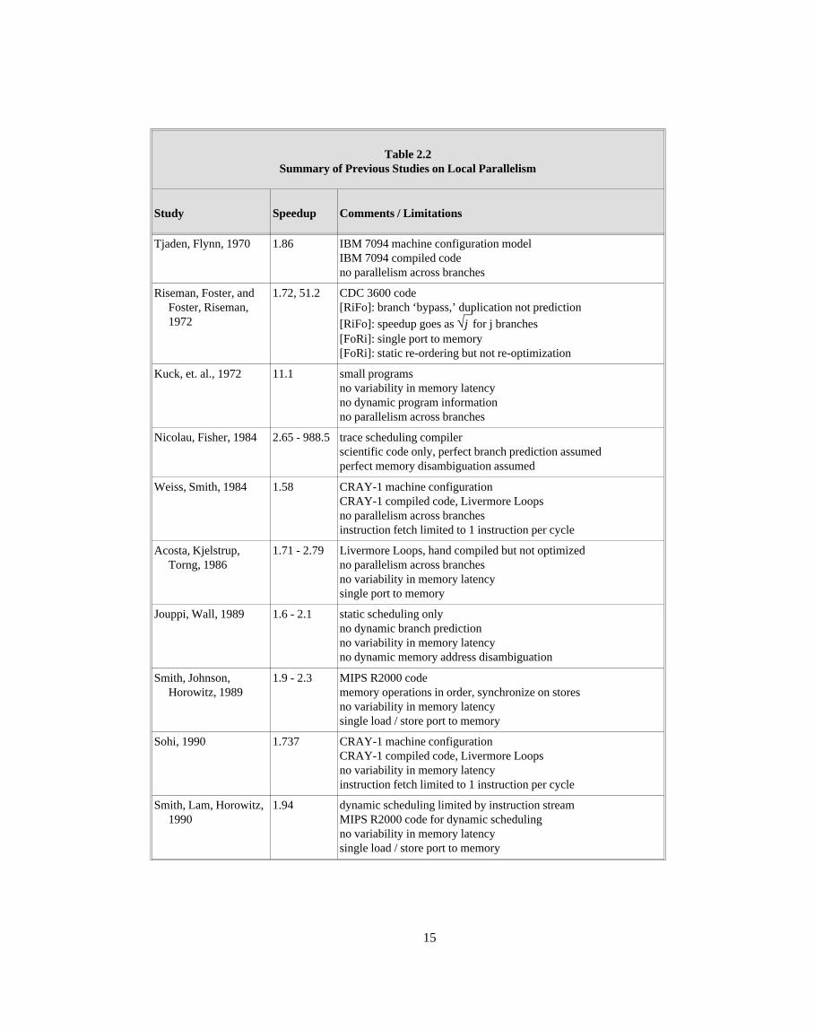
Table 2.2Summary of Previous Studies on Local Parallelism

Study Speedup Comments / Limitations

Tjaden, Flynn, 1970 1.86 IBM 7094 machine configuration modelIBM 7094 compiled codeno parallelism across branches

Riseman, Foster, andFoster, Riseman,1972

1.72, 51.2 CDC 3600 code[RiFo]: branch ‘bypass,’ duplication not prediction[RiFo]: speedup goes as √j for j branches[FoRi]: single port to memory[FoRi]: static re-ordering but not re-optimization

Kuck, et. al., 1972 11.1 small programsno variability in memory latencyno dynamic program informationno parallelism across branches

Nicolau, Fisher, 1984 2.65 - 988.5 trace scheduling compilerscientific code only, perfect branch prediction assumedperfect memory disambiguation assumed

Weiss, Smith, 1984 1.58 CRAY-1 machine configurationCRAY-1 compiled code, Livermore Loopsno parallelism across branchesinstruction fetch limited to 1 instruction per cycle

Acosta, Kjelstrup,Torng, 1986

1.71 - 2.79 Livermore Loops, hand compiled but not optimizedno parallelism across branchesno variability in memory latencysingle port to memory

Jouppi, Wall, 1989 1.6 - 2.1 static scheduling onlyno dynamic branch predictionno variability in memory latencyno dynamic memory address disambiguation

Smith, Johnson,Horowitz, 1989

1.9 - 2.3 MIPS R2000 codememory operations in order, synchronize on storesno variability in memory latencysingle load / store port to memory

Sohi, 1990 1.737 CRAY-1 machine configurationCRAY-1 compiled code, Livermore Loopsno variability in memory latencyinstruction fetch limited to 1 instruction per cycle

Smith, Lam, Horowitz,1990

1.94 dynamic scheduling limited by instruction streamMIPS R2000 code for dynamic schedulingno variability in memory latencysingle load / store port to memory

15

unlimited number of additional registers were added, the code being simulated had already been

compiled and optimized for a machine with only a few registers and function units. Finally, this

study did not consider exploiting parallelism across conditional branches.

In a similar analysis, Foster and Riseman in [FoRi72] consider a modified CDC 3600. They did

not allow parallelism across basic blocks but the did allow an unlimited number of function units.

Also, they discuss the ability of the compiler to re-order instructions within a basic block to improve

scheduling. They concluded that a speedup of 1.72 was possible. One limitation with this study is

that the optimizations applied to the static code are strictly re-ordering of instructions that the 3600

compiler had already generated. They don’t allow the compiler to re-optimize the basic block for

the additional registers and function units. Also, there is still only a single port to memory.

A companion note [RiFo72] considers the effect of ‘bypassing’ conditional jumps by executing

streams in parallel. This is not equivalent to dynamically predicting branches and executing only a

single stream of code. They conclude by saying that:

“ Our results seem to indicate that even very large amounts of hardware applied to programsat run time do not generate hemibel improvement in execution speed.”

Thus, even though their results showed that speedups of on the average 51.2 were possible, they

discounted this as being too hardware intensive. However, this conclusion is based on the assumption

that all parallel paths of a branch must be executed simultaneously. The authors did not consider

dynamic branch prediction to allow this parallelism to be taken advantage of by only executing a

single path. They had an interesting conclusion, empirically based, that the speedup grows as the

square root of the number of branches that are bypassed.

Kuck et al. measured parallelism available on FORTRAN programs in [KuMC72] and [KBCL74].

In this study, a program was broken into basic blocks which were then optimized and analyzed for

potential speedup. The results were then averaged together to get an overall speedup for the program.

Unlike the previous two studies, the static optimization of the basic blocks was fairly extensive,

employing tree height reduction techniques to decrease the total time required to compute a block.

Many of these techniques create additional operations in the process and in fact, the average operation

16

redundancy Rp over all programs in the study was 2.4.

There are several limitations to this study. First, the programs being studied were very small, most

of them less than 40 FORTRAN statements and when present the number of loop iterations was

usually less than 10. It is not clear how this group of small pieces of programs, especially when

averaged together, relate to a single program running on real data from beginning to end. Another

limitation is that memory was not handled very realistically. It was assumed that the memory could

be cycled in unit time (which is the time for all ALU operations) and that there were never any

accessing conflicts. Further, for most of the data presented this constraint was included for memory

stores only. That is, all memory fetches were assumed to be overlapped with ALU operations. While

ignoring instruction stream fetches is reasonable for this type of analysis, the interaction between

data memory fetches and ALU operations is a critical aspect to instruction level parallelism,

especially in consideration of cache misses and bank conflicts.

The third limitation of the this study is that no dynamic program information was included. All

paths through the program which were determined statically were averaged together with equal

weight.

“ Thus, we assume that each trace is equally likely, an assumption required by the absence ofany dynamic program information. We feel this assumption yields conservative values, sincethe more likely traces - which are probably large and contain more parallelism - are givenequal weight with shorter, special case traces.”

This is certainly believable, but it is not clear how one could even attempt to speculate how

conservative the data is. Also, the absence of dynamic information eliminates the possibility of taking

advantage of dynamic memory disambiguation. Potential conflicts between memory operations

must be made more conservative than is required. The final limitation is that inter-basic block

parallelism is not exploited. Each basic block is analyzed separately and the results are averaged

together. However, it should be noted that the technique applied to what are called IF tree blocks in

effect exploits some parallelism across conditional branches. A group of small basic blocks are

combined into a single unit with a multi-way branch. It is related somewhat to the basic block

enlargement techniques discussed in chapter 4.

17

Weiss and Smith analyze instruction issue logic in [WeSm84]. Using the Lawrence Livermore

Loops compiled for the CRAY-1 in scalar mode, they simulate several different schemes for issuing

instructions. These include fully sequential, where instructions are started in instruction stream order,

to a tag forwarding scheme where instructions are allowed to issue out of order. They conclude that

the maximum theoretical speedup is on the average 1.58.

This study was concerned mainly with the effect of adding functionality to a CRAY-1 rather than

the effect of tag forwarding techniques in general. Thus, it is not clear how much relevance the study

has to other machine configurations. No additional ports to memory or function units are simulated,

and no techniques are used to exploit parallelism across branches. Further, the scheme simulated

does not take full advantage of tag forwarding:

“ We treat the register files B and T as a unit, with one busy bit per file, since it is not practicalto assign tags to so many registers.”

Also, the memory address disambiguation scheme uses dynamic information but does not allow

memory accesses to schedule out of order. In addition, performance was limited by allowing a

maximum of one instruction to be fetched per cycle. This may be a valid constraint for a machine

which has to implement the CRAY-1 architecture, but does not represent a fundamental constraint

on the issuing scheme. Finally, since scientific benchmarks (Livermore Loops) were used, these

results may be too optimistic for general purpose code which may have greater branch densities.

Nicolau and Fisher in [NiFi84] analyze speedup for VLIW machines. They conclude that speedups

anywhere from 2.65 to 988.5 are possible over the range of benchmarks chosen. This paper analyzes

a strictly static approach to parallelism discovery. Using a technique called trace scheduling, basic

blocks are enlarged and parallelism is exploited over a large part of the program. This technique is

similar in concept to the basic block enlargement we discuss in chapter 4 except that here it is strictly

static. This means that all branches must be known statically and that fix-up code is needed in branch

destinations that are not optimized for. As we will show later, when basic block enlargement in used

in conjunction with dynamic branch prediction, neither of these restrictions are necessary. Another

limitation of strictly static approaches is that memory disambiguation must be static. This study

18

assumed that two memory references could always be disambiguated statically.

In a similar study, Acosta, Kjelstrup and Torng in [AcKT86] analyzed an instruction issuing

scheme to allow multiple out of order instructions to be issued per cycle. They evaluated Livermore

Loops under a variety of machine configurations and concluded that speedups ranging from 1.71 to

2.79 were possible. The benchmarks were hand compiled for each of the machine configurations,

but the code was not highly optimized:

“ In hand-compiling the benchmarks, a ‘‘dumb’’ compiler has been assumed. Such a compiler,although being simple, fast and reliable, is not capable of improving the code it generates usingcomplex optimizations. For instance, redundant subexpressions and redundant loads are notremoved.”

In addition, the memory model was limited. Only a single port to memory was simulated and the

memory access delay was fixed. Also, there was no parallelism exploited across branch instructions.

In the conclusions they make the following remark:

“ ... dynamic scheduling in hardware can free compilers of burdensome static schedulingdecisions.”

This represents a common myth about dynamic scheduling. As we will show later in this dissertation,

far from removing a burden from the compiler, dynamic scheduling can actually places more of a

burden, albeit in different ways.

In [JoWa89] Jouppi and Wall present the results from an analysis of instruction level parallelism

in addition to providing some definitions. VLIW machines are mentioned along with three distinc-

tions between superscalar and VLIW, all of them related to instruction stream format:

• the fixed format of VLIW machines makes decoding easier

• the fixed format wastes bandwidth with NOPs in sequential code

• the fixed format ties the object code to a particular implementation

They then go on to say that these distinctions are not very significant and so VLIW does not need to

be considered separate from superscalar. These points of comparison suggest a limited concept of

a superscalar machine. They are focusing on machines in which operations are compiled into a

single stream and the issue logic decides if multiple operations can be issued in parallel, stalling if

19

they cannot be. They do have this interesting comment, however:

“ We will not consider superscalar machines or any other machines that issue instructions outof order. Techniques to reorder instructions at compile time instead of run time are almost asgood, and are dramatically simpler than doing it in hardware.”

As we will demonstrate later, out of order execution can have very significant performance

advantages in some circumstances. This paper goes on to show that instruction level parallelism

ranges between 1.6 and 3.2. Their conclusion is thus that current machines already exploit most of

the parallelism available:

“ Thus for many applications, significant performance improvements from parallel instructionissue or higher degrees of pipelining should not be expected.”

This analysis has three limitations. The first, as mentioned above, is dynamic scheduling. The

second limitation, closely related to the first, is dynamic branch prediction. The authors mention

loop unrolling (which is equivalent to static branch prediction) and show the advantages it can achieve

on scientific code, but say that these techniques are “of little use on non-parallel applications like

yacc or the C compiler.” This may be true, but it is important to know how much use dynamic branch

prediction is on a dynamically scheduled machine. The third limitation has to do with the memory

model. They analyze only pipelines with fixed, predictable latencies. As we will demonstrate later

in this dissertation, when memory is modeled more realistically, scheduling issues become more

significant. The lack of dynamic memory address disambiguation also reduces the potential number

of memory operations that can be scheduled.

Smith, Johnson and Horowitz discuss limits on parallel instruction issue in [SmJH89]. They use

instruction traces from a MIPS R2000 and simulate a machine with a similar function unit and

memory configuration. Out of order execution is allowed and an unlimited number of registers are

added through register renaming. They simulate both two unidirectional ports to memory as well as

2 load ports and 1 store port. They conclude that a speedup of little more than 2 is achievable in most

circumstances.

The memory model used in this study was that of a perfect cache. First, there was no variability

in memory latency. Also, all memory accesses were issued in order, and stores were issued only

20

after all previous instructions have completed. Without more information, it is hard to know how

much this memory system limitation has limited performance. Also, note that the study used traces

from a processor with a single port to memory, and that there were no static optimizations applied

to the code. One of the main points of this study, however, was the influence of instruction fetch

limitations on performance. We do not consider instruction bandwidth issues in this dissertation, but

many of the issues that Smith et al. focus on are strictly related to the instruction stream format.

Unless one is constraining oneself to a re-implementation of an existing architecture, some of these

limitations disappear. There is no fundamental reason, for example, that branch targets should not

be made available at the beginning of a basic block, rather than when the actual test operation is

encountered. This yields more time to predict and fetch target locations. Branch target alignment is

also trivial to accomplish with a small cost in code space.

In [Sohi90] Sohi analyzes instruction issue mechanisms for the CRAY-1 running the Livermore

Loops. This study is similar to [WeSm84] in experimental methodology. Sohi uses non-vectorized

compiled code for the CRAY-1 and limits the issue rate to 1 instruction per cycle. He proposes a

mechanism which allows out of order execution, exploits parallelism across branches and does

dynamic memory disambiguation. He concludes that a maximum speedup of 1.737 is achievable on

average. We have already mentioned the problem associated with using code compiled for a specific

machine configuration on a machine with more resources. Since the CRAY-1 was used as a model,

there is only a single port to memory and in addition it was assumed that no memory bank conflicts

occurred. Finally, the result bus which carries function unit results back to the register file was only

allowed to transfer one value per cycle.

The last study we will consider is [SmLH90], where Smith, Lam and Horowitz analyze a technique

to apply dynamic branch prediction to a statically scheduled processor. Speedup is analyzed over a

variety of machine configurations, and a value of 1.94 is reported as its maximum value. The main

problem with this paper is that it is unfair in what it claims is a comparison of how a statically

scheduled processor with dynamic branch prediction would compare to a dynamically scheduled

21

processor (also with dynamic branch prediction).

Dynamic branch prediction, by incorporating backup structures, allows parallelism to be exploited

more easily across conditional branches. No fix-up code is needed and run-time information can be

used to predict branches. We will discuss this further in chapter 4. These advantages are present

whether dynamic branch prediction is applied to dynamic or static scheduling. Given a statically

scheduled processor with dynamic branch prediction, the main advantage a dynamically scheduled

processor would still have is the ability to better handle variability in memory latency and to perform

dynamic memory address disambiguation. The authors make the following claims about the short-

comings of dynamic scheduling:

• hardware is complex

• only a small window can be analyzed

• branch point misalignment hurts

The last point is an instruction stream format issue, it has nothing to do with the scheduling discipline

of the hardware. The authors seem to have a limited definition of dynamic scheduling. They explain

dynamic scheduling by saying:

“To maintain scalar code compatibility, all instruction scheduling is done by the hardware.”

In fact, the concept of dynamic scheduling has nothing to do with scalar code compatibility. There

is no reason a dynamically scheduled processor cannot take advantage of the same things a statically

scheduled processor can (e.g. the ability of the compiler to optimize over large pieces of code, the

use of static branch prediction information and the ability to format the instruction stream in a way

that is efficient to fetch).

Further clouding their results is the fact that the performance data for the dynamically scheduled

processor comes from instruction traces of a MIPS R2000 while the data from the statically scheduled

machine is compiled and optimized for the new implementation. Also, the paper considers only a

single port to memory and there is no variability in memory latency. Related to this the authors make

the following remark:

“ Though real caches will have a definite effect on the relative performances, we believe that

22

caches should affect both machines in similar ways.”

We will show in chapter 6 that for a single port to memory, the effect is indeed fairly small. However,

as we allow multiple memory nodes to be scheduled each cycle, the difference between static and

dynamic scheduling becomes more pronounced.

23

Chapter 3 Models of Execution

In this chapter we present two models of execution: the interface model and the atomic unit model.

These models are two different perspectives on the design and operation of a single instruction stream

processor. They characterize aspects of a processor that are relevant to the issues being addressed

in this dissertation. They are presented to provide a framework for the microarchitectural mecha-

nisms discussed in the next chapter.

The interface model focuses on the different interfaces present in a processor. The interface of

main interest is the dynamic/static interface. We define this interface and illustrate how it is distinct

from the hardware/software interface. The dynamic/static interface is important in clarifying the

tradeoffs between dynamic and static scheduling. Often this issue is confused with others from which

it is independent.

The atomic unit model introduces the notion of different collections of work that are indivisible

in certain respects. The atomic unit of primary interest is what we call the execution-atomic-unit.

We define this concept along with the concept of the compiler-atomic-unit and the architectural-

atomic-unit. The atomic unit model provides a framework for the discussion of basic block

enlargement in the next chapter.

3.1 The Interface Model

A computer can be thought of as a multilevel system with high level algorithms at the top and

circuits at the bottom. In between are levels, or interfaces, which define sets of data structures and

the operations allowed on them. Examples of interfaces are high level languages, machine languages

and microcode.

The number and nature of these interfaces varies widely from system to system. Indeed, a circuit

could be designed to implement a specific algorithm, in which case there need not be any intermediate

interfaces. In practice, however, complex designs are specified hierarchically. Thus, there are usually

24

interfaces defined even within a dedicated unit. In fact, a hardware device, for example a logic gate

or a transistor, could itself be thought of as an interface.

An interface is a specification. What takes place at an interface and when it takes place depends

on the type of interface and how it is used. A widely discussed interface is the hardware/software

interface (HSI) which defines the boundary between hardware and software. Another interface, not

as widely discussed but more important, is the dynamic/static interface (DSI), which defines the

boundary between translation and interpretation. We will compare and contrast these two interfaces

in this section. First some terms will be defined, followed by an historical background. We will then

discuss some basic tradeoffs associated with the DSI and provide some configuration examples.

3.1.1 Definitions

The dynamic/static interface (DSI) arises from the fact that algorithm solutions typically undergo

two stages. In the first stage, translation, the specification of the algorithm is changed from one

format into another. That is, a new algorithm specification is created at a different interface. This

new specification contains all of the information needed and the old specification is no longer

required. In the second stage, interpretation, the algorithm specification is executed, using input data

that is not part of the specification, and results are generated. The DSI is this interface between

translation and interpretation.

In practice the distinction between translation and interpretation can be a bit fuzzy. For example,

suppose an algorithm has no input data. It could be argued that the execution of the algorithm is

actually part of the translation process, where the algorithm is being translated into its output. In this

case the interpretation of that algorithm would be just to print the output. Conversely, suppose a

program is compiled only once and then run, it might be argued that there is no translation and that

the compilation process is part of the interpretation of the algorithm. The compiled code in this case

could be viewed as a run-time generated intermediate form. Thus, two concepts are important for

the definition of the DSI:

• a problem specification separate from the input data

25

• a solution which can be applied repeatedly on different sets of inputs

By requiring this second point, we can distinguish translation activities as those that take place

only once. Consider, for example, a processor that translates the instruction stream into a more

convenient form and saves that form internally. Is this process translation or interpretation? By our

definition this is interpretation, because, even though the process occurs before dynamic binding

takes place, it will take place each time the program is run. Thus, it is important to distinguish an

external problem specification, which exists separate from the processor, from internal processor

state, which merely involves the caching of translated code. In all of the benchmarks used in this

dissertation, there was a clearly defined translation and interpretation process, and the input data was

easily distinguishable from the algorithm itself.

In contrast to the dynamic/static interface is the hardware software interface (HSI). The definition

of the HSI is even more problematic than that of the DSI. The question of what is hardware and what

is software does not have a simple answer. The extremes are easy to identify, but the distinction is

less clear in between. The crucial element in the way these two terms are generally considered is the

question of alterability. In other words, how easy it is to alter a particular process is related to how

soft the related interfaces are. We will not attempt a formal definition of hardware and software, and

thus we will leave the definition of the HSI purposefully vague. The problem with a firm definition

is that the exact conditions under which a process can be altered would have to be specified: would

one have to return the processor to the factory?, replace hardware in the field?, power cycle the

processor?, halt execution momentarily?, etc...

But consider the following notions. The microcode of most machines, even though it may be

stored in read/write memory, is probably more correctly viewed as hardware because it cannot be

changed without halting the processor. Even the microcode of the IBM System/370 model 145,

which is stored in main memory, obeys this definition because the memory region containing the

microcode is protected and cannot be changed without rebooting [Katz71]. However, the microcode

of machines such as the B1700 [OrHi78] and the QM-1 [RaTs70] should probably be thought of as

26

software because it can be modified while the processor is running. In the case of a machine with a

built in translator, it would be appropriate to place the HSI at the translated-from interface as long

as the translation process cannot be modified.

The DSI and the HSI are distinct interfaces. The former is concerned with translation and

interpretation, the latter with alterability. However, in the majority of situations the DSI and the HSI

are identical. For conventional machines running compiled languages, the DSI is at the machine

architecture level. The high level language program is translated into machine language, which then

gets interpreted by the hardware. The HSI is also at this level because the processes below the

machine architecture cannot be altered while those above can.

Suppose we have a program that interprets a high level language. In this case, the DSI is above

the machine architecture level, at the interface defined by whatever intermediate language is being

interpreted. But the HSI is still at the machine architecture level because the interpretation process

can be altered. The DSI is above the HSI. An opposite example is a case where hardware translates

a program from one interface to another. The translation process is not alterable, therefore the HSI

would be at the interface which is translated from. But the DSI will be at the interface which is

translated to as long as the problem specification is saved externally, separate from the processor’s

internal state. Thus, the DSI is below the HSI in this case.

The main interface of interest from a performance point of view is the DSI, not the HSI.

Translation and interpretation are important issues, alterability is less so. However, the terms

hardware and software have certain legal ramifications independent from their engineering ones.

One way to define the terms that has nothing to do with alterability can be found in [PaAh85]. Patt

and Ahlstrom argue there that microcode should be considered hardware if it is provided by the

manufacturer and software if it is written by the user. This concept is distinct from those of the HSI

and DSI described above. It might be called the builder/user interface: defining the boundary between

what the builder provides and what the user has access to.

27

3.1.2 Historical Background

The connection between the concepts of hardware vs. software and translation vs. interpretation

has not been made in a coherent manner. In this section, we will provide a brief background on how

others have viewed the DSI and the HSI and to what extent they have connected the two. People

have long recognized the two-phase nature of the execution of most programs. Hoevel [Hoev74]

addresses the DSI directly and argues that it should optimally be at an intermediate level. Flynn

[Flyn80], [Flyn83] also distinguishes the DSI. These papers, however, do not discuss the DSI in

connection with the HSI.

Myers, in chapter 3 of [Myer80], compares some basic approaches to computer architecture. He

distinguishes five approaches: traditional, language-directed, type A HLL machines, type B HLL

machines and type C HLL machines. The main feature separating these approaches is the level of

the DSI, not the level of the HSI. The discussion centers on the translation and interpretation process,

even though the terms ‘‘machine architecture’’ and ‘‘machine language’’ are used, which suggest

an alterability concept. The implicit assumption is made that the HSI and DSI are the same with the

exception of type B HLL machines, which differ from type A machines only in that the HSI is higher

(above the DSI).

Myers discusses a category in which the hardware translates as well as interprets, but he seems to

consider the ‘‘machine architecture’’ in this case to be the level from which interpretation takes place

rather than the level from which translation takes place:

“ Note that the type B machine has the same semantic gap as a type A machine. Its onlyadvantage over a type A machine is that the assembly process should be faster because it isimplemented as a microprogram or in hardware.” ;

This would imply that he considers the DSI to define the semantic gap. However, in his discussion

of hardware vs. software, he seems to be talking about something else:

“ Architects often use the following three criteria in determining whether a function should beimplemented in the machine rather than in software: (1) the function should be small, (2) the

28

; [Myer80], p. 46

function should be unlikely to change, and (3) system performance would suffer from a slowersoftware implementation of the function.” ;

These criteria are not related to the translation and interpretation issue and the second criterion

clearly relates to a question of alterability. Thus, Myers shows that the HSI and the DSI (by our

definitions) are separate things, even though he does not discuss them in this way.

Tanenbaum in [Tane84] separates the DSI from the HSI more clearly although he does not connect

the two together. In Chapter 1, multilevel machines are introduced and the techniques of translation

and interpretation are defined. He does not mention the DSI explicitly, but he does discuss translating

to and interpreting from different levels (i.e., movement of the DSI). Then, software and hardware

are discussed:

“ Any operation performed by software can also be built directly into the hardware and anyinstruction executed by the hardware can also be simulated in software. The decision to putcertain functions in the hardware and others in the software is made on the basis of such factorsas cost, speed, reliability, and frequency of expected changes.” :

Thus, these two common textbooks in computer architecture illustrate how the DSI and HSI have

not been clearly distinguished. It is important when considering tradeoffs to know whether the

relevant interface is the HSI or the DSI. Alterability is important from an engineering standpoint

when considering issues such as cost, reliability or frequency of expected changes. However, when

considering strictly performance, it is mainly the DSI that is relevant. This point is explained more

fully below.

3.1.3 DSI Tradeoffs

To illustrate how performance is a DSI and not an HSI concept it is helpful to consider as an

example integer multiplication. Suppose we analyze the behavior of a program and determine that

multiplies by small integers are very common. One approach to improved performance is to remove

from interpretation those things which can be pre-computed at translation time. Thus, if the compiler

29

; Ibid.: [Tane84], p. 11

can determine statically when the multiplies by small integers occur and what values they have, we

could potentially improve the speed of the overall computation (depending on the relative speed of

addition and multiplication) by explicitly doing the shifts and adds that are necessary. This involves

moving functionality across the DSI. We have taken a higher level of interpretation (the multiply

instruction) and replaced it with lower level steps.

Now consider another scenario. Suppose we have a processor in which there is no integer

multiplication at the architecture level. If the problem calls for a multiplication, the compiler has to

generate individual shift and add instructions. We might analyze our processor and determine that

an atomic multiply instruction could operate faster than individual shift and add steps. Again this

involves movement of functionality across the DSI. It is the creation of a larger granularity unit (the

multiply instruction) as a single interpreted function which allows performance to be optimized. It

could be the case that microcode within our enhanced processor will emulate the multiply instruction

by doing shifts and adds at the same speed as they would otherwise have occurred. In this case, we

have moved the DSI but have not capitalized on that movement. Alternatively, we may have installed

a hardware multiply function unit which does a multiply with fewer propagation delays than separate

shifts and adds. Thus, we need to distinguish two different processes going on:

• the movement of functionality across the DSI (from interpretation to translation or fromtranslation to interpretation.)

• the optimization of the interpretation of a function specified at the DSI.

The second step is a basic step involved in the design of a processor. Once the DSI has been chosen,

it is straightforward engineering to evaluate the frequency of individual functions and optimize the

performance of those that are used most frequently. These two steps are closely interrelated. The

first step will depend on what will be done in the second step and vice versa. Note that even though

these two steps both involve the DSI, HSI movement tends to be related with the second one. This

is because often the optimization of an interpreted function will involve as side-effect a reduction in

the alterability of that interpreted process.

30

Further complicating the interrelationship between these two steps is the fact that the complexity

of the compilation process is involved. An unsophisticated compiler would suggest a different DSI,

and thus would cause the interpretation process to be optimized differently than would a sophisticated

compiler. Two level interpreters are also difficult to analyze. In this case, the highest level interpreter

would be executing instructions which would themselves be interpreted by a lower level interpreter.

Note that the problems associated with translating to the lowest of the two levels are different from

the problems associated with writing an interpreter which executes above this level. Thus, it is not

always straightforward to compare the compilation to microcode with the creation of a macrocode

interpreter in microcode.

There are also bandwidth tradeoffs. Lower level DSI’s may increase the run-time bandwidth to

the highest level interpreter. Raising the DSI would lower the bandwidth required to this interpreter,

and since the lower level interpreters are generally smaller, this could be advantageous.

3.1.4 DSI Placement Examples

Figure 3.1 shows a diagram of different configuration examples and how they involve DSI

placement. The vertical axis does not represent an exact parameter. It would be difficult to place

an interface on a single dimensional scale; here we only intend to abstractly illustrate the processes

involved. However, it would be possible to formalize this axis by defining some appropriate measure

of complexity. An example would be the total number of gates required for the execution of a

program. We could dynamically measure the number and type of each operation which gets executed

at a particular interface over the course of a program. Then the number of gates required for each

operation would be averaged.

The first example represents a conventional interpreter. The high level language program gets

translated into an intermediate level code. Then it gets interpreted by a program running on a

conventional microprogrammed machine. There are three levels of interpretation involved: the

intermediate level code by the machine level code, the machine level code by the microcode and the

microcode by the gates. In the next example we show a conventional microprogrammed machine

31

running compiled code. In this case the intermediate code step is eliminated and the compiler

translates directly to the machine language level. This eliminates the third level of interpretation.

Dynamic microprogramming in a concept which has the same DSI placement as this conventional

compiled code case but lowers the HSI. The motivation behind dynamic microprogramming is to

allow the DSI to be better matched to the problem being run. By lowering the HSI, the level in

between the HSI and the DSI becomes alterable, thus the DSI can be changed for different problems

being run. Examples of dynamic microprogramming are the Burroughs B1700 series [OrHi78] and

the QM-1 [RaTs70].

Intermediatecode

Instruction SetArchitecture

Microcode(single cycle

level)

IndividualGates

High LevelLanguage

High LevelLanguage Machine

Conventional Machine

withInterpreter

Conventional Machine

withCompiled

Code

Compilationto

Microcode

HighPerformance

Processorwith

CompiledCode

Figure 3.1DSI Placement Examples

32

Cook and Flynn describe a dynamically microprogrammable computer in [CoFl70], and Flynn,

Neuhauser and McClure describe the EMMY system at Stanford in [FlNM75], which was similar.

Also, the ‘Interpreter’ is described in [ReFF72], a system similar to the QM-1. Rauscher and

Agrawala discuss the application of dynamically microprogrammable machines in [RaAg78]. Most

of these papers and books, however, do not explicitly address the issue of DSI placement. The main

point behind dynamic microprogramming is HSI placement, not DSI placement. That is, the goal is

to make the lower level process alterable in order to tune the machine to different problems being

run. It is generally assumed that the DSI should be where it typically has been in similar

microprogrammed machines. In other words, these machines are generally designed as interpreters,

they are not set up to handle placement of the DSI at the HSI (compiling down to the microcode

level).

Taking an opposite approach from dynamic microprogramming is vertical migration. The

principle here is to optimize the interpretation of some sequence of operations, generally raising the

HSI in the process. In some cases the DSI is raised with the HSI, and in some cases it remains

unchanged. The difference lies in whether the functions that are vertically migrated are then

translated to, or are then used by an interpreter. In other words, it could be a sequence of operations

which are themselves part of an interpreter which are being combined into a single optimized unit

or it could be a sequence of operations which are part of a translated file. In either case, the motivation

behind this idea is to eliminate redundant operations within a sequence of commonly executed

functions. Performance is also increased because of reduced instruction bandwidth. Raising the HSI

is usually associated with this because the new function is generally not alterable. The implementor

of the functions which were vertically migrated had a finer level of control than would be possible

using constructs above the HSI. In the typical example, functions that were previously written in the

macrocode of a conventional processor are rewritten in microcode, which then becomes part of the

hardware.

33

Hassit and Lyon describe an application of vertical migration in [HaLy76] and [HaLL73]. This

was a vertical migration of selected APL primitives. The primitives were microcoded on an IBM

System/370 model 25. Weber describes an implementation of EULER on an IBM System/360 model

30 in [Webe67]. Luque and Ripoll provide a summary and overview of vertical migration in

[LuRi81]. Pihlgren describes the vertical migration of COBOL primitives in [Pihl80]. These are just

a few examples of the many papers published in this area.

The next example in figure 3.1 involves the compilation to microcode or to an interface with a

low level of complexity. This could be thought of as representing reduced instruction set machines.

Of course, there is no consensus on what defines a reduced instruction set machine. We consider in

this example only those machines that put the DSI and the HSI at the lowest level possible, since this

is the critical issue. Examples of these machines are the IBM 801 [Radi83], the Berkeley RISC

[Patt82], [PaSe82], the Stanford MIPS [HJGB82], [HJPR82], and the HP Spectrum [BiWo86],

[MCFH86].

The basic feature of the reduced instruction set idea is to lower the DSI as well as the HSI. The

dynamic microprogramming idea discussed above advocated the lowering of the HSI, but not the

DSI. Some papers justifying the ‘reduced instruction set’ concept seem to gloss over the fact that the

DSI is lower as well as the HSI. For example, Radin, in [Radi83], makes the following statement

with regard to the IBM 801:

“ ... the benefits claimed [of microcode] are generally not due to the power of the instructionsas much as to their residence in a high-speed control store. This amounts to a hardwarearchitect attempting to guess which subroutines, or macros, are most frequently used andassigning high-speed memory to them. ... The 801 CPU gets its instructions from an ‘instructioncache’ which is managed by least recently used information. Thus, all frequently used functionsare very likely to be found in this high-speed storage, ...” ;

Birnbaum and Worley also make an equivalent remark about the HP Spectrum family. : What they

fail to make clear is that the DSI has been lowered as well as the HSI. Making the comparison

34

; [Radi83], p. 237: [BiWo86], p. 41

between a control store and an instruction cache is not as simple as they might have you believe

because one has microinstructions below the DSI and the other has microinstructions above the DSI.

These are two very different situations and a comparison is not simple. Besides, some computers

cache the control store without lowering the DSI, for example the Burroughs B1726 [OrHi78]. The

hit ratio of a control store cache depends only on the frequency of individual instructions. The hit

ratio of an instruction cache depends on instruction stream locality, compiler technology, and how

dynamic the environment is.

The next DSI placement example represents a higher performance version of the second example.

Here, the microcode interpreter has been eliminated and the machine language level is executed

directly. There are many issues involved in such a machine. First, the instruction set architectures

of many processors do not lend themselves to hardwired implementations. If the architecture was

designed with a microprogrammed state machine model in mind, it can be difficult to convert it into

a more appropriate data flow graph model. Most high performance versions of microprogrammed

machines have a significant amount of hardware support for high frequency instructions. Some

instructions may be executed in a single cycle through the use of special hardware while others may

go through a many cycles sequence. Thus, the distinction between the second and fourth examples

is not always so clear.

Alternatively, if the instruction set architecture is designed specifically with a hardwired im-

plementation in mine, the distinction between the third and fourth examples becomes fuzzy. Making

this distinction involves some analysis of the complexity of the interfaces, which is difficult at best.

In the next section we introduce a model which can make these distinctions clearer by focusing on

different levels of atomic units of work.

The last example in figure 3.1 is the high level language machine. In this case the HSI is raised to

the high level language level. The DSI is also generally raised as high as possible, usually to an

intermediate level below the HSI. The SYMBOL machine was an early example of this [RiSm71],

[SRCL71], [Rice81]. In this case, the HSI is at the SYMBOL language level [Ditz81] since the

35

hardware is able to accept SYMBOL language input, while the DSI is at a slightly lower level

represented by the internal representation of a SYMBOL program. The hardware of the machine

translates a SYMBOL program into this intermediate form (removes redundant blanks, changes

keywords into bit strings, replaces symbolic addresses to pointers, etc.). After this translation has

been completed for the entire program, execution begins.

Another example of a high level language machine is the Abacus machine that ran BASIC

[BuFS78]. Like SYMBOL, this machine has the HSI at the high level language level and the DSI

slightly below. Abacus did a hardware translation similar to that performed by SYMBOL before

starting the execution of the program. A FORTRAN machine [BaSK67] also falls into this general

category. The HSI is at the FORTRAN level, the DSI is slightly below. Finally, there is a machine

proposed by Chu and Abrahms [ChAb81], [Chu79]. Unlike the previous examples, we would place

the DSI for this machine actually at the high level language level. During the execution of the

program, the hardware actually scans the source code and executes it. No translation is done prior

to this, and there exists no other specification of the program other than the source code. (Note,

however, that a processor with the DSI at the high level language level could internally cache a

translated portion of the program.)

3.2 The Atomic Unit Model

In this section we discuss the notion of an indivisible unit of work, or an atomic unit. An important

property of the model discussed in this section is that the atomic units have a defined size. The way

atomic unit size is defined is not critical as long as it is consistent. In this section we will talk about

the size of an atomic unit in terms of the number of nodes that implement the atomic unit.

Conceptually, a node is the most primitive unit the processor can execute, for example a simple

arithmetic operation, a load or a store. The exact set of nodes that any given processor implements

is different, but it will not be important for the purpose of this section to identify the set of nodes

explicitly. We have identified three separate types of atomic units: architectural-atomic-units,

36

compiler-atomic-units, and execution-atomic-units. We define each of them below and then discuss

tradeoffs associated with their sizes. Finally we present some examples of CAU/EAU configurations.

3.2.1 Definitions

A compiler-atomic-unit (CAU) is the smallest indivisible unit of work that the compiler generates.

These may be individual nodes or they may be larger units of work. For example, if a compiler

generates an instruction which does a register relative load (a constant is added to a register and the

memory contents at that address are loaded into another register), this would represent a CAU with

a size of two nodes. The instruction is indivisible because the compiler does not specify the add node

explicitly (even if it could have using other instructions).

An architectural-atomic-unit (AAU) is that set of nodes which is atomic with respect to interrupts

and exceptions. By definition, the state of the process being executed can only be preserved at an

architectural atomic unit boundary. The specification of these units is relevant to interrupt latency

and exception handling. For most processors, AAU’s are the same as individual machine instructions

(i.e. CAU’s). Interrupts and exceptions are only handled at instruction boundaries. AAU’s could also

be larger than CAU’s (if some instruction boundaries were defined to be un-interruptible) or smaller

than CAU’s (if some machine instructions could be interrupted). The latter would be the case for

block move instructions which can be interrupted and restarted where the left off (e.g., if a page fault

within an instruction causes the instruction to be continued rather than restarted).

Note that temporary results that are used only within an AAU do not have to be named explicitly.

That is, the output of one node can go directly to the input of another node without going through an

explicitly named register, allowing fewer general purpose registers to be architecturally specified.

Thus, larger architectural-atomic-units potentially decrease the size of the architectural state of the

machine, making context switching less expensive.

In the case of machines with imprecise exceptions the concept of an architectural-atomic-unit is

not well defined. Suppose that a floating point multiply followed by a load is defined in such a way

that if the multiply generates an exception, the load may have already occurred when the exception

37

handler is entered. In this case, there is no clear unit of work which is atomic with respect to

exceptions. The point at which exceptions are taken depends on the sequence of instructions that

gets executed. For the purpose of this section, we consider only processors which implement precise

exceptions.

Execution-atomic-units (EAU’s) are groups of nodes that get executed together as a single unit.

An EAU is indivisible in the sense that the processor cannot execute only part of it. If some event

occurs which prevents the EAU from being terminated normally, the processor backs up, throwing

away the entire EAU. In most machines, the EAU’s are the same as the AAU’s (which are in turn

the same as the CAU’s). The use of imprecise exceptions is analogous to increasing the EAU size

beyond the size of the CAU’s. The hardware is simpler because individual instruction boundaries

are not always preserved. In the next section we discuss tradeoffs between atomic unit sizes more

fully.

3.2.2 Atomic Unit Tradeoffs

Since exceptions are architecturally defined at AAU boundaries, this is where most processors

also place EAU’s. The processor thus implements precision at this level. An AAU either completes

or is backed up. AAU’s and EAU’s do not have to match but allowing the EAU’s to increase beyond

the size of the AAU’s is non-trivial and requires the implementation of some sort of backup hardware.

In the event that an AAU boundary in the middle of an EAU needs to be preserved, the backup

hardware restores the state of a machine to the beginning of the EAU. Execution then proceeds down

a different path.

But why bother with such a scheme? As we will show in the next chapter, there are some good

reasons to have large EAU’s. Enlarging EAU’s to the size of basic blocks is fairly straightforward.

(A basic block is that unit of work in between branch instructions.) We will show how EAU’s can

also encompass multiple basic blocks. In this case, branches that are within an EAU must be verified

at run-time, causing backup if they fail. Thus, minimum hardware requirements are a scheme that

allows backup to the start of the EAU and the ability to efficiently execute branch confirmation nodes.

38

We call EAU’s which encompass embedded branch fault instructions enlarged basic blocks. This

concept is discussed more fully in the next chapter.

Larger EAU’s allow parallelism to be exploited over a larger instruction window more efficiently.

The compiler is able to optimize and schedule more operations as a single unit. It may be possible

to eliminate work which was previously computed more than once due to register limitations. Also,

larger EAU’s allow an increased utilization of issue bandwidth. That is, by allowing a larger unit of

work to be packed together, it is easier to maximize the rate at which work is entered into the data

path. This has increased significance for dynamically scheduled machines, where the packing of

work is only limited by EAU size, not by data dependencies.

An important issue that relates to this advantage has to do with compiler-atomic-units. It is

important to consider the degree to which the CAU’s are matched to the to the implementation. The

CAU’s may be fairly independent from an exact implementation, or alternatively they may be

formatted exactly into the set of nodes which get issued into the machine on each cycle. If the

execution-atomic-units are larger than compiler-atomic-units, the mechanism for packing compiler-

atomic-units into execution-atomic-units becomes an important issue. This packing can either be

done at translation time or at run-time. If the compiler-atomic-units are formatted to match the

implementation, as would be the case for a statically scheduled machine or for some dynamically

scheduled machines [HwPa86], the compiler does the packing statically. If, however, the compiler-

atomic-units are independent from the implementation the packing must be done dynamically. This

might be the case if a buffer against changes in technology is desired or if an existing architecture is

being implemented. We refer to the hardware that does this kind of packing as a ‘fill unit.’ We

describe one potential implementation of a fill unit in chapter 5.

3.2.3 CAU and EAU Size Examples

Figure 3.2 illustrates some examples of different CAU and EAU sizes. In the case that the compiler

specifies individual nodes, then the CAU size will be equal to one. All three points on the left fall

into this category. If alternatively the compiler specifies units of work that encompass multiple

39

nodes, the CAU size would be larger, for example four as illustrated. The diagonal line represents

machines in which the CAU’s and EAU’s are equal in size. Conventional processors lie on this line.

In the lower left is an example of a machine with a low level instruction set architecture (individual

nodes) and a processor which executes the nodes as individual units. Such a processor may employ

many performance enhancing techniques, but the EAU size is equal to one because all instruction

node level ISA,high performance

processor withspeculativeexecution

node level ISA,low performance

processor

high level ISA,no speculative

execution

node level ISA,high performance

processor, nospeculativeexecution

Ave

rage

Num

ber

of N

odes

per

EA

U

2 4

1

2

8

1

16

4

Average Number of Nodes per CAU

Figure 3.2CAU Size vs. EAU Size Examples

40

boundaries are preserved by the hardware. The machine at the other end of this line would be one

in which individual instructions contain multiple operations.

Moving up vertically is the case of a CAU size of one and an EAU size of four. This would be

the case for a processor that allows the compiler to specify individual nodes but only preserves

atomicity at a larger level, for example each basic block. This would be the case for a processor with

overlapped execution within a basic block but no speculative execution. At the upper left is the case

where EAU’s are allowed to encompass multiple basic blocks. This requires a processor that supports

speculative execution and has some sort of backup hardware. In the next chapter we discuss

mechanisms related to processors with multiple basic block EAU’s.

41

Chapter 4 Microarchitectural Mechanisms

This chapter draws on the two models discussed in the previous chapter and describes various

choices in the design of a microarchitecture. We define microarchitecture as what is below both the

HSI and the DSI, as discussed in the previous chapter. That is, we are only interested in that part of

the processor that is not alterable and directly interprets a problem specification. If hardware

translates the program to a new specification before execution, we do not consider that here; if a

processor executes a program that is itself an interpreter of a higher level machine language, we will

consider only the lowest level interpreter. However, we do consider mechanisms where a processor

translates an instruction stream into a different form internally.

In this chapter we first discuss the concept of local parallelism and then present three

microarchitectural mechanisms that are the subject of this dissertation: dynamic scheduling, dynamic

branch prediction and basic block enlargement. Dynamic scheduling involves the decoupling of

nodes from others with which they are issued. This decoupling permits nodes to be scheduled to

function units when their operands are ready and not prevent others from being scheduled when their

operands are not. Dynamic branch prediction involves the use of speculative execution to exploit

parallelism across basic block boundaries. Basic block enlargement is a technique which works in

conjunction with dynamic branch prediction to allow the basic blocks as executed by the hardware

to be larger than those which are specified by the program.

4.1 Local Parallelism

We define local parallelism as parallelism that exists within a small window of the dynamic

instruction stream. It is only this parallelism that a single instruction stream processor can take

advantage of. Global program transformation techniques can be used to exploit other kinds of

parallelism. One example is by converting a program into multiple instruction streams and utilizing

multiple processors. We assume for the purposes of this dissertation that, from the point of view of

42

single processor, there still exists a sequential control-flow oriented instruction stream, and in this

case local parallelism is all that is available.

Consider the overall parallelism available in an application. Parallelism is a characteristic of the

overall problem that is being solved. That is, the definition of the problem permits certain things to

take place simultaneously. The parallelism that exists at this highest level must be discovered before

it can be used. This discovery can take place at many different levels: at the algorithm level, at the

program level, at the machine code level and at the individual node level. Exactly what discovering

parallelism means is different for translations (above the DSI) and for interpretations (below the

DSI).

Above the DSI, discovering parallelism means translating to an interface in which parallelism is

explicitly represented. For example, a programmer may take an algorithm specification and create

several independent subroutines in some parallel programming language. In this case, the program-

mer has discovered the parallelism in the algorithm by translating it into explicitly parallel pieces of

code. Another example would be a compiler that creates vectorized code in which pipelining is

explicitly represented. The compiler has discovered the parallelism by taking what had been a

sequential loop and translating it into an interface in which pipelined operations are specified

explicitly.

Thus, to discover parallelism above the DSI, the interfaces being translated to must have some

way to represent parallel operations. Then, the translations or interpretations at lower levels know

explicitly what is independent. This parallelism can be exploited in a straightforward manner. But

creating a interface that represents parallelism is non-trivial. In addition, most of the effort that has

gone into these higher level translations (i.e. algorithm design, programming language design and

machine language design) has been toward sequential models.

Thus, translations typically involve a reduction in the degree of apparent parallelism. For example,

the algorithm designer decides on a sequence of steps which need not actually occur one after another

to solve the problem; or the programmer decides on a sequence of statements which may occur in

43

parallel and still satisfy the algorithm; or the code generator translates into a sequence of machine

instructions in the same way. Parallelism that is hidden in this way is not necessarily lost forever.

It may possibly be discovered at lower levels, either by other translators or by interpretations.

Discovering parallelism below the DSI is a different issue. Here, the idea is to take operations

defined in a sequential model and dynamically allow overlap to occur. That is, the higher level

translator has created units of work which semantically occur with no concurrency and the lower

level interpreter applies concurrency to them. As we showed in Chapter 1, virtually all processors

do this to some extent. A simple execution pipeline in which the hardware guarantees data

dependencies is the simplest form of this type of discovery. More complex processors which do

branch prediction and dynamic scheduling are other examples.

It is important to distinguish parallelism discovery from parallelism exploitation. In order to

exploit parallelism, it must have first been discovered, but it only has to be discovered once. Thus,

if the compiler has generated code in which parallelism is explicitly represented, the processor may

exploit a great deal of parallelism, even though it may not be doing any actual discovery. For

example, if a compiler vectorizes loops for a vector machine, the parallelism discovery has occurred

during translation. The hardware then just needs to execute the sequence of instructions potentially

with a high degree of parallelism. The issue of parallelism discovery by the compiler versus the

hardware is one of the issues involved in dynamic versus static scheduling.

4.2 Dynamic Scheduling

Dynamic scheduling is a microarchitectural mechanism where the group of nodes that are currently

active are decoupled from each other. Thus, the set of nodes that are issued together is not necessarily

the same as the set that gets scheduled. This mechanism has been implemented and proposed in

many variations. As discussed in chapter 2, the tag forwarding scheme of the IBM 360/91 originated

the core idea behind dynamic scheduling [Toma67]. Keller extended the idea and provided more

background in [Kell75].

44

The HPS concept of restricted data flow, generalized the concept of tag forwarding to encompass

all operations within a processor, including memory operations, and with enough backup state to

allow dynamic branch prediction and precise exceptions. HPS was was introduced in 1985

[PaHS85], [PMHS85] and is being reported on in continuing research [PSHM86], [PMHS86],

[HwPa86], [Hwu87].

The alternative to dynamic scheduling is static scheduling (scheduling at compile-time) These two

choices are not mutually exclusive; most processors use some of both techniques. One principal

advantage of dynamic scheduling over static scheduling is that it allows individual nodes to be

scheduled when they are ready to be executed and without holding up other nodes when they are not.

In the face of variable memory latency (i.e. cache misses) and the ability of the hardware to

disambiguate memory addresses at run-time, this decoupling of nodes can lead to the discovery of

valuable parallelism. The other main advantage of dynamic scheduling is that it allows parallelism

across basic blocks to be exploited more efficiently.

In the case of pure static scheduling, the pipeline of the computer is exposed and the compiler fills

in the node slots based on the static instruction stream. All memory operations are assumed to have

a specific fixed latency (the cache hit latency) and there is a simple hardware interlock to stall the

pipeline on a cache miss so that the forwarding of results within the pipeline works properly. The

compiler preserves the original sequence of memory nodes in which there is a possible address match.

Standard optimizations, such as register renaming, common sub-expression elimination and node

un-chaining are performed by the compiler within a basic block, but no optimization crosses basic

block boundaries. There is no backup hardware and exceptions are imprecise.

In the case of dynamic scheduling, there are no restrictions on the ordering of the nodes within

the basic block as generated by the compiler. The machine issues all the nodes fully decoupled from

one another, and any node result can be forwarded to any other node. Nodes are allowed to wait for

memory or ALUs as long as necessary for their operands to become ready. The exact order of the

execution of the nodes within the basic block is not determined. It may depend on memory cache

45

contents and/or run-time operand values. Thus, exceptions within the basic block must either be

specified as imprecise or some sort of backup hardware must be present. This backup hardware if

present allows basic block boundaries to be precise. If finer granularity of precision is needed, the

machine may allow nodes to schedule at a slower rate. When dynamically scheduled processors

have backup hardware, usually dynamic branch prediction is also implemented because of the ability

to efficiently handle branch prediction misses. (We will show in the next section however that

dynamic branch prediction is an independent concept and can be applied to statically scheduled

processors as well.)

There are several reasons that prevent statically scheduled machines from filling pipeline slots as

effectively as dynamically scheduled machines. The first is variability in memory latency. When a

memory read takes a cache miss, the statically scheduled machine must stall and wait for the data

even if there are other operations that are available to be performed. In machines with few resources

this may not impose a significant performance penalty. Only if there is other work that can be done

within the instruction window will dynamic scheduling pay off. A simple improvement to pure static

scheduling allows memory reads to be pre-loaded. This means that if a memory read causes a cache

miss, a stall is not generated until the result is actually needed. This requires slightly more

sophisticated hardware but can be a significant advantage if the compiler is able to schedule reads

early enough to prevent stalls in most cases.

Another reason dynamically scheduled machines can fill pipeline slots more fully has to do with

memory address disambiguation. Because the compiler only has static information available, it has

to make a worst case assumption about matching memory addresses. Even if two memory nodes

rarely or never point to the same location, the compiler is forced into imposing an artificial

sequentiality unless it can determine no match will occur. An example of this is the case of array

accesses with indices computed at run-time. Dynamically scheduled machines can do memory

disambiguation at run-time and schedule the memory operations as appropriate to guarantee data

flow dependencies are maintained.

46

Of course, dynamic memory disambiguation hardware can be added to a statically scheduled

machine and in fact some sort of hardware like this usually present in all processors. In order to

pipeline memory accesses, even if they occur in program order, it is necessary to have some checking

logic to preserve data dependencies. This logic can then introduce stalls only when needed rather

than the alternative which is to force no overlap of memory accesses. However, in the presence of

out of order ALU operations and multiple ports to memory, a bigger advantage can be achieved by

allowing memory accesses to occur out of order while still preserving flow dependencies.

Note that the ability of a statically scheduled machine to take full advantage of an execution

pipeline depends to a large extent on the resources available. In the case that there is only one port

to memory and one ALU, it is unlikely that there will be much difference in performance between

static and dynamic scheduling. Also note that branch prediction becomes important here. Dynamic

scheduling can take advantage of dynamic branch prediction more effectively by allowing parallelism

to be exploited across basic block boundaries. We discuss dynamic branch prediction more fully in

the next section.

Consider as an analogy a hardware cache. The fundamental principle behind a cache, as opposed

to an explicitly managed local storage, is to dynamically schedule memory locations onto fast

temporary storage. In cases where:

• the environment is very stable (e.g. one program has control of the entire CPU), and

• the code has predictable memory accessing behavior (e.g. large arrays being accessed inknown patterns), and

• the number of executions of a single program is high (i.e. it is cost effective to spend a lot ofeffort compiling)

a fast local storage that is managed by the compiler may be more appropriate than a cache. The

compiler and/or assembly language programmer can determine statically good choices for which

memory locations should be scheduled onto the faster local storage. A selection is made that is as

good as or better than that a cache could make, and without the cost (in hardware and/or time) of a

47

cache lookup for every access. This is probably why Cray chose this option in the Cray 2. The jobs

running on this machine generally fit these three criteria.

However, when these conditions do not hold, a cache starts looking better. That is, if the

environment is multitasking (more than one program is using the CPU), or the memory accessing

behavior is less predictable, a hardware cache is generally much more appropriate. The hardware

LRU algorithm can make a much better selection dynamically of which memory locations should

be scheduled onto fast local storage and the additional cost is small in comparison to the speedup

achieved.

This same idea can be extended to scheduling of nodes onto function units. If the branches are

highly predictable (statically speaking) and the memory latency has a very low variance (either no

cache or very high hit ratio) and memory addresses are known statically, a compiler can schedule

nodes onto function units just as well as a dynamically scheduled microengine. Nodes can come

from the static instruction stream, access the register file and go directly through to the function units

without any waiting. Thus, there is a lowered hardware cost and a potential speedup due to a possible

reduction in latency.

However, in more dynamic situations the tradeoffs change. If the branches are significantly more

predictable at run-time than at compile time or if the memory latency has an appreciable variance or

if memory addresses are hard to disambiguate statically, dynamically scheduled techniques can make

a better determination of which nodes should go to which function units than the compiler. How

much better and at what cost is one of the main topics of this dissertation and will be addressed in

the next chapter. It is important to realize that static and dynamic scheduling are just two ends of a

spectrum. Even with dynamic scheduling hardware, the compiler can do things which allow the

hardware to discover more parallelism (e.g. increasing the size of the basic blocks, as we will see

below).

48

4.3 Dynamic Branch Prediction

In this section we will discuss dynamic branch prediction. We define dynamic branch prediction

in a way slightly different from its popular use. Conventionally, dynamic branch prediction refers

to a mechanism in which run-time information is used to predict the direction of branches. This is

opposed to static branch prediction in which the compiler predicts branches using static information.

The question over whether static or dynamic information is used to predict branches is secondary to

performance. The real issue is whether or not a dynamic action it taken; that is, if speculative

execution is supported.

In the remainder of this dissertation, we will define dynamic branch prediction as a mechanism

in which branches are predicted so that operations are allowed to be merged into the machine before

the results of the prediction are confirmed (regardless of whether or not run-time information was

used to predict the branch). Conversely, static branch prediction is defined as predicting branches

before dynamic binding occurs. This might be the case in which branch prediction is used as a hint

for the pre-fetcher to lower instruction fetch delay. Thus, by our new definitions, both dynamic and

static branch prediction may or may not use run-time information to predict the branches.

Dynamic branch prediction implies some form of backup capability. This is used in the case that

a branch is predicted incorrectly. Note, however, that this backup logic may be very simple, it may

consist of simply the ability to squash a write, flush the pipeline and re-fetch along another path. The

manner in which dynamic branch prediction is able to increase performance depends on whether the

microarchitecture employs static or dynamic scheduling.

In the case of a purely statically scheduled machine without dynamic branch prediction, delay

slots are usually implemented. These are used to overlap the pipeline delay of confirming a branch

direction. Typically, the instruction immediately following a branch instruction is executed regard-

less of which direction is taken (in some cases the following two instructions). The compiler tries

to fill the delay slot with work from the basic block being branched from or from one of the basic

blocks being branched to. Ideally, the delay slot can be filled that must be performed regardless of

49

branch direction. In some cases, however, it may only be possible to fill the delay slot with work that

is only needed in one direction of the branch. Filling the delay slot this way sometimes requires the

insertion of addition instructions in the alternate branch path to undo the effect of this work. This is

called fix-up code and can be advantageous if the optimized branch direction is executed much more

frequently than the alternate one. Finally, it may be necessary for the compiler to insert a NOP if no

appropriate work can be found for the delay slot.

If dynamic branch prediction is added to a statically scheduled machine such as we have been

describing, there are several advantages. First, delay slots can be filled more effectively. Operations

may be placed into these locations that will get undone if the branch is taken a certain way. Also,

this obviates fix-up code in the alternate basic block. In fact, moving operations up from a favored

branch path could apply to slots within the basic block other than the branch delay slot. This may

require more complex backup hardware, however. In order to be able to backup an entire basic block,

typically an alternate or shadow register file is maintained and writes to memory are buffered in a

write buffer before they are committed. We will show in the next section that with hardware such

as this, basic blocks can be enlarged beyond their normal size to further increase pipeline slot

utilization.

While statically scheduled machines can take advantage of dynamic branch prediction as we have

shown, the use of dynamic branch prediction in a dynamically scheduled machine is a much more

powerful concept. Here, the issuing of operations continues across conditional branches and thus all

work within several adjacent dynamic basic blocks contends for data path resources. (However, we

will show in the next section how the use of basic block enlargement techniques allow statically

scheduled machines with dynamic branch prediction to get some of these advantages.)

This use of dynamic branch prediction in conjunction with dynamic scheduling in this way

introduces the concept of the instruction window. The instruction window represents a window of

the dynamic instruction stream. The instruction window can be defined in several ways. One way

is to count the number of active basic blocks. An active basic block is one that has been partially or

50

fully issued (i.e. entered into the data path) but not retired (i.e. finalized with no possibility of being

undone). We can also measure the window size by the number of nodes in a particular state. For

example, the number of active nodes, the number of ready nodes or the number of valid nodes. A

node in the machine is always valid between when it is merged and when it is retired. It is active up

until when it is scheduled and it is ready only when it is active and schedulable.

4.4 Basic Block Enlargement

In chapter 3 we defined execution-atomic-units as those units of work which are executed as an

atomic unit. We saw that these units are distinct from the smallest units that the compiler generates

and from those that are supported at the architectural level. The concept behind large execution-

atomic-units is to allow more parallelism to be exploited. By allowing the hardware to consider a

larger group of work to be an uninterruptible unit, more work can be overlapped. The basic block

enlargement techniques we will describe in this section involve the exploitation of dynamic branch

Fault: <addr>

Fault: <addr>

Trap:

Address #1 Address #2Basic Block Type

‘trap’ assert node; eitherexecutes silently or signals and

causes the two-way branchprediction to be reversed,

discarding all future basicblocks but retaining this one.

‘fault’ assert nodes; eitherexecute silently or signal andprovide an address to jump to

after discarding this basicblock and all future ones.

Figure 4.1Sample Basic Block Structure

51

prediction to increase the size of the execution-atomic-units. We will consider the static and dynamic

scheduling cases separately.

Suppose we have a statically scheduled processor with dynamic branch prediction and the ability

to execute an entire basic block before committing the work. As we discussed in the previous section,

this allows the compiler to move work into unused pipeline slots without having to insert fix-up code

in the alternate path. But the compiler need not stop with only a single basic block. Several basic

blocks could be combined into a single unit, re-optimized and then generated as a single entity for

execution. In this case, at run-time this enlarged basic block would contain several embedded branch

tests to confirm the branch prediction was correct. This is essentially what trace scheduling [Fish81]

involves except in that case there is no dynamic branch prediction (i.e. no speculative execution and

no backup hardware), so the compiler must be more conservative. Loop unrolling and software

pipelining are also examples of enlarging basic blocks in the absence of dynamic branch prediction.

Figure 4.1 shows a sample basic block for a hypothetical machine with dynamic branch prediction.

Here we introduce the concept of an assert node, which is like an ordinary ALU operation except

T: X,Y

T: P,Q

T: B,C

T: X,Y

F: ABT: P,QF: AC

AC

A

AB

B C

entry

entry

Figure 4.2Basic Block Enlargement Example

52

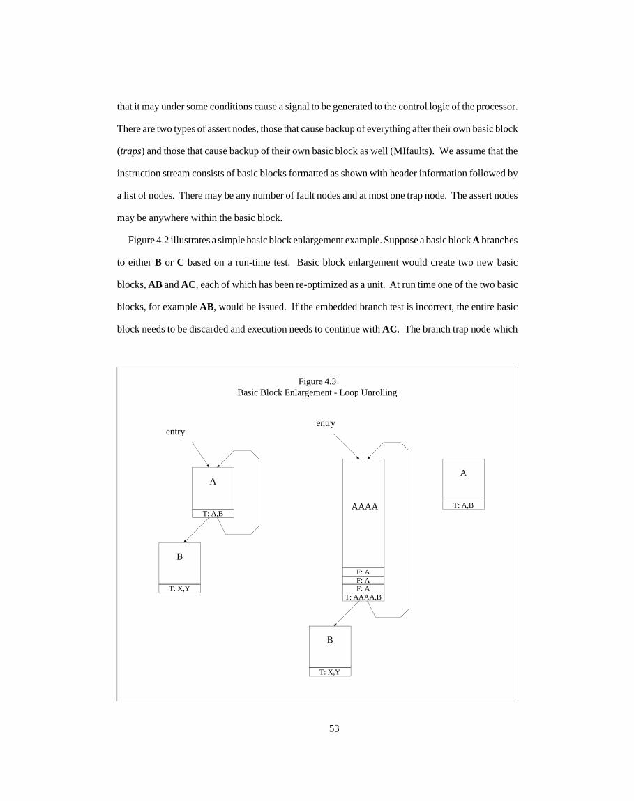
that it may under some conditions cause a signal to be generated to the control logic of the processor.

There are two types of assert nodes, those that cause backup of everything after their own basic block

(traps) and those that cause backup of their own basic block as well (MIfaults). We assume that the

instruction stream consists of basic blocks formatted as shown with header information followed by

a list of nodes. There may be any number of fault nodes and at most one trap node. The assert nodes

may be anywhere within the basic block.

Figure 4.2 illustrates a simple basic block enlargement example. Suppose a basic block A branches

to either B or C based on a run-time test. Basic block enlargement would create two new basic

blocks, AB and AC, each of which has been re-optimized as a unit. At run time one of the two basic

blocks, for example AB, would be issued. If the embedded branch test is incorrect, the entire basic

block needs to be discarded and execution needs to continue with AC. The branch trap node which

T: X,Y

T: A,B

T: AAAA,B

F: A

A

AAAA

B

entryentry

Figure 4.3Basic Block Enlargement - Loop Unrolling

F: A

F: A

T: A,B

A

T: X,Y

B

53

previously was part of A has been retained, but it has been converted to a fault node and been given

an explicit fault-to location. Note that in the case that the AC basic block is never entered directly,

the fault node could be eliminated. This is because the only way to get there would be the fault node

in AB. Thus, there is no need to make the test that is guaranteed to succeed. However, if code which

previously branched to A can potentially branch to AC, then the fault node needs to be retained. The

concept of doing fault prediction to automatically update the entry basic block is discussed in chapter

7.

This process of basic block enlargement can be continued recursively, allowing the creation of

arbitrarily large basic blocks. Note that multiple iterations of a loop can be overlapped in this way,

as shown in figure 4.3. In this case, there is a choice of whether or not to generated intermediate

stages of basic blocks. For example, in the case that only the third fault node in the AAAA basic

block signals, we could immediately fault to a AAAB basic block. Faulting back to the A basic block

will require more work to be re-done but it will save code space and basic block generation time. In

the case the the loop is executed many times, it will probably only be worthwhile to generate the

single enlarged basic block. The choice of which basic blocks to enlarge and in which way is

complex. We envision a classification of branches into three categories:

• dynamic use is low; enlargement is not worthwhile

• dynamic use is high and the direction is highly weighted toward one particular directionknown at compile time (e.g. loop tests)

• dynamic use is high and the direction is not highly weighted toward one particular direction

If a branch falls into the second category, the branch path would be optimized in one direction

only. If a branch falls into the third category, both directions would be optimized. It is also important

to create boundaries of enlarged basic blocks in such a way that discarding work is unlikely. For

example, branches within an enlarged basic block are ideally correlated with one another. Employing

optimizations along multiple paths implies a slightly more complex branch prediction mechanism

than would otherwise be required. Generally we would want a specific path (i.e. a specific enlarged

basic block) to be re-executed on re-fetching of the same entry point.

54

4.5 Dynamic Scheduling / Basic Block Enlargement Tradeoffs

Consider how basic block enlargement would apply to dynamically scheduled machines. A

natural question that arises is why basic block enlargement is needed with dynamic scheduling. Since

multiple basic blocks are merged into the machine, parallelism can already be exploited across

conditional branches. Why then, is there an advantage to having the compiler (or possibly a hardware

fill unit) create larger basic blocks? There are two reasons: larger scale optimization and issue

bandwidth. First consider issue bandwidth. A problem that arises with basic blocks small relative to

the number of operations that can be issued in a single cycle is that of low utilization of issue slots.

The solution is to allow a larger unit of work to be packed into the set of nodes issued as a unit. In

this way, the machine does not starve due to not being able to get enough work into it. In a machine

Figure 4.4Decoupling / Enlargement Tradeoff

(all branches 95% hit rate, mutually independent)

Window

ModerateEnlargement,

Few ActiveBasic Blocks

ExcessiveEnlargement,Single ActiveBasic Block

NoEnlargement,Many ActiveBasic Blocks

.90 .86 .81 .77 .74 .70 .66 .63

.86 .74 .63

.63

.95

.95 .95 .95 .95 .95 .95 .95 .95.95

.86 .86 .86

higherexecutionefficiency;

fewerdiscardedoperations

betterpacking of

basic blocks;higher

utilization ofissue

bandwidth

issue rate>>

schedule rate

issue rate =

schedule rate

55

which can merge 16 nodes in a single cycle running code with basic blocks that are are only 5-6

nodes large, this is obviously a critical technique.

The second reason for having basic block enlargement with dynamic scheduling has to do with

the optimization of basic blocks. By combining two basic blocks across a branch into a single unit

and then re-optimizing it as a unit, a more efficient basic block is achieved than would be created by

just putting one after another. Extending the example of chapter 2, suppose a compiler generates

code like this:

p <-- p + 4a <-- mem[p]jump to XYZ if (a > 0)

XYZ: p <-- p + 4 b <-- mem[p]

If the two basic block are enlarged across this branch, the artificial flow dependency through p

can be eliminated. If the two basic blocks were issued separately, this would be nearly impossible

to detect.

Thus, dynamic scheduling benefits by basic block enlargement. Now the opposite question arises:

given basic block enlargement, why do we need dynamic scheduling? The main reason is that basic

block enlargement cannot take advantage of parallelism as flexibly as dynamic scheduling. Figure

4.4 illustrates the tradeoff that exists between dynamic scheduling and basic block enlargement. As

we have already seen, small basic blocks lead to problems with issue bandwidth and large scale

optimizations. At the other extreme, a single enlarged basic block (as in the case of static scheduling)

suffers from low efficiency. Each branch fault node within the enlarged basic block has a certain

probability of causing backup. For large basic blocks running non-scientific code, there is a point

where efficiency will fall off to the point that enlargement is no longer worthwhile. The chances of

having to discard a basic block are high enough that it does not pay to make it larger.

The application of dynamic scheduling on top of basic block enlargement allows work with high

probability of being needed (early in the window) to coexist with work with lower probability of

being needed (late in the window). In a statically scheduled machine, the issue rate and the schedule

56

rate are identical. Thus, all work in the machine has the same probability of being needed. In a

dynamically scheduled machine the issue rate can exceed the schedule rate. Thus, we have basic

blocks being merged into the machine faster than their associated branches can be confirmed.

57

Chapter 5 The Abstract Processor Model

In this chapter we introduce the abstract processor model. It captures the relevant aspects of the

class of single instruction stream processors that are the subject of this dissertation. This model

implements the microarchitectural mechanisms discussed in the previous chapters and is used as the

subject of the simulation study described in the following chapter.

The model is abstract because it does not represent a single specific implementation of a processor.

Certain characteristics are allowed to vary over a range of possibilities and others are left unspecified.

In the first category are variables the effect of changing which is measured. For example, the model

accommodates both static and dynamic scheduling, which have quite different hardware require-

ments. The second category is for variables which do not apply to the measurements under study.

For example the instruction set architecture is not specified. The focus of the model is on the manner

in which operations are scheduled onto function units. The manner in which these operations are

encoded in the static instruction stream and the manner in which they are decoded by the hardware,

while important issues in their own right, are not being addressed.

In this chapter we use the term node to refer to the most primitive arithmetic or memory operation,

for example a simple two’s complement addition or a single read from memory. The execution of

a node may take many machine cycles, but it is the smallest unit for which explicit input operands

and results are specified. In the abstract processor model we have defined a set of memory and ALU

nodes which operate on the underlying 32-bit data path. Most nodes have two 32-bit inputs and a

single 32-bit output, but we have also defined some double nodes which have four 32-bit inputs and

two 32-bit outputs. The complete list of nodes implemented along with their latencies and dynamic

usage for all benchmarks is shown in Appendix A.

We also use the term multinodeword in this chapter to refer to collections of nodes which are

processed in the same cycle. Nodes are combined into multinodewords in two places in the machine:

as the set of nodes that are issued in the same cycle (an issue-multinodeword) and as the set of nodes

that are scheduled for execution in the same cycle (a schedule-multinodeword). In the case of a

58

statically scheduled machine, the issue and schedule multinodewords are the same since issuing and

scheduling are the same process. In the case of a dynamically scheduled machine, the two are

different. When the term is used without qualification, we are refering to issue-multinodewords.

In this chapter and in the following one, we restrict the analysis to situations in which a high level

program is compiled into machine language and then executed. The performance that we are trying

to optimize involves only the execution of the program after it has been compiled. As we pointed

out in chapter 3, there are other factors that are relevant in some circumstances. For example, in

cases where there is no logical division between the program and the input data or where a program

is compiled only once and then executed, the distinction between compile-time and run-time is a

little unclear. Even further clouding the issue would be a situation where parts of the program are

compiled only as needed or even altered and then re-compiled dynamically.

This chapter is divided into five sections. In the first section we give an overview of the abstract

processor model. The second section describes the instruction unit. This portion of the processor

fetches the static instruction stream, does all necessary sequencing, including branch prediction, and

provides decoded nodes to the node tables. In the third section we describe the scheduling unit, which

contains the node tables and alias tables. This portion of the machine is responsible for handling all

data dependencies and performing all scheduling decisions. The fourth section describes the

execution unit which contains the ALUs. In the last section we describe the memory unit, which

handles memory address disambiguation and write buffering in addition to forming the interface to

the memory system.

5.1 Model Overview

Figure 5.1 shows an overall block diagram of the abstract processor model. It is divided into four

units: the instruction unit, the scheduling unit, the execution unit and the memory unit. The box on

the left of the diagram represents system memory and is not part of the processor itself. This memory

is divided into two pieces: the static instruction stream and the data memory. These pieces are

addressed separately and the instruction stream cannot be modified by the program itself. This

59

multiple pipelined function units

EUNITSchedule-multinodewordsMUNIT

GeneralPurposeRegisters

andRegister

AliasTable

dynamic register values oraliases get merged with

multinodewordsIssue-multinodewords

Node Tableand

Scheduling Logic(dynamic

scheduling only)

Distribution Bus(distribution of node results)

addresstranslation

unit

data cacheand

write buffer

IUNITMemory System

Figure 5.1Abstract Processor Model Overview

StaticInstruction

Stream

InstructionCache

(optional)

Fill Unit(optional)

NodeCache

(optional)

DataArea

SUNIT

Basic Block Sequencer

60

restriction was added mainly to avoid unnecessary complications. In an actual processor, the

instruction stream would have to be writable, in an unrestricted way or perhaps requiring some level

of privilege.

Within the instruction unit the instruction stream may go through decoding, translation and/or

caching. It may be cached before the decoding and translation stage as well as after. We refer to the

hardware that packs a freely formatted instruction stream into multinodewords as a fill unit. We

consider the use of a fill unit to be optional because the model allows it to be present but does not

require it. In some cases, the static instruction stream may pass through unchanged and go directly

into the sequencer. In this case, the only function being performed by the instruction unit would be

the processing of control instructions and the handling of backup. In other cases, a complex fill unit

may convert an encoded instruction stream into nodes, pack the nodes into multinodewords, and then

apply basic block enlargement on top of that. We discuss the various options for the instruction unit

more fully in the next section.

The basic blocks sequencer interprets the control instructions in the instruction stream and

sequences the basic blocks using branch prediction. Each basic block contains one more more assert

nodes, which will signal if a branch prediction miss occurs or execute silently otherwise. An assert

node is an simple arithmetic operation, like a compare, that makes a test at run-time and has the

additional information of which direction the associated branch was predicted. For non-enlarged

basic blocks, a single assert node is placed at the end of the basic block representing the prediction

for the following basic block. In this way, a branch prediction miss is a trap rather than a fault because

the basic block containing the assert node is valid. In the case of enlarged basic blocks, however,

there may be many assert nodes within the basic block. All of these will cause faults if they signal,

except the last one, which will be a trap node as usual.

In the case of a statically scheduled machine, the issue-multinodewords sent out by the IUNIT are

the same as the schedule-multinodewords sent out by the SUNIT. That is, as the multinodewords

leave the basic block sequencer they go directly into the function units. The compiler has already

61

guaranteed that dependencies will be met. In this case, the only synchronization that the hardware

performs is to guarantee memory latency. The compiler has scheduled based on a predicted memory

latency. Whenever memory is slower than this, the machine is stalled until the result arrives.

In the case of a dynamically scheduled machine, a node table in the SUNIT is present as well as

register alias logic. Each node that has been issued waits in the node table decoupled from the other

nodes in the same issue-multinodeword. When all of the node’s source operands are ready and an

appropriate function unit is available, the node gets sent to the EUNIT or the MUNIT. The register

alias table is used during the merging process to enforce flow dependencies and remove anti and

output dependencies. In this case the hardware does all synchronization, both for memory and

arithmetic units.

The distribution bus is used for the results of memory reads and arithmetic nodes. Results are

distributed both to the register alias table and to the node table (if present), where other nodes may

be awaiting these results as source operands. In the case of static scheduling, the register alias table

consists only of the architecturally visible registers. Results are permitted to be distributed directly

to the inputs of function units, bypassing the node table if there are no older ready nodes to schedule.

This bypass logic, critical to high performance, is implemented for both static and dynamic

scheduling.

A pipeline diagram is shown in figure 5.2. The three activities associated with the processor are:

merge, schedule and distribute. In the merge phase newly created nodes are stored in the node tables,

in the schedule phase the oldest ready node in each node table is selected for execution and in the

distribute phase the node tables and alias tables are updated with the results of completed nodes. A

simple implementation of this pipeline would introduce an extra cycle of latency in order to get into

and out of the node tables. We implement a pipeline bypass here to allow distributing results to go

directly to the inputs of function units. In the case of dynamic scheduling the node table is being

bypassed and the scheduling logic must handle this case. In the case of static scheduling, it is the

62

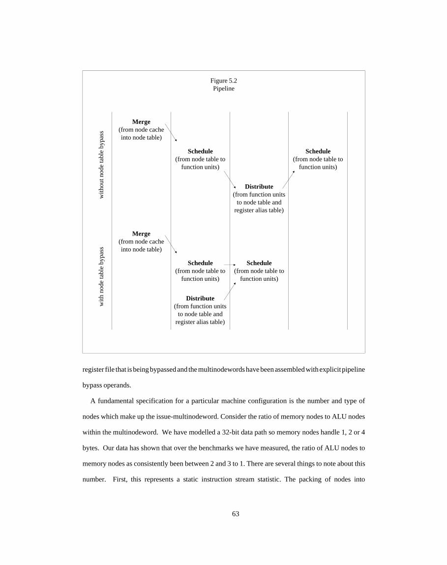
register file that is being bypassed and the multinodewords have been assembled with explicit pipeline

bypass operands.

A fundamental specification for a particular machine configuration is the number and type of

nodes which make up the issue-multinodeword. Consider the ratio of memory nodes to ALU nodes

within the multinodeword. We have modelled a 32-bit data path so memory nodes handle 1, 2 or 4

bytes. Our data has shown that over the benchmarks we have measured, the ratio of ALU nodes to

memory nodes as consistently been between 2 and 3 to 1. There are several things to note about this

number. First, this represents a static instruction stream statistic. The packing of nodes into

Merge(from node cacheinto node table)

Schedule(from node table to

function units)

Distribute(from function units

to node table andregister alias table)

Figure 5.2Pipeline

Schedule(from node table to

function units)

Distribute(from function units

to node table andregister alias table)

Schedule(from node table to

function units)

Schedule(from node table to

function units)

Merge(from node cacheinto node table)

with

nod

e ta

ble

bypa

ssw

ithou

t nod

e ta

ble

bypa

ss

63

issue-multinodewords, whether it is done by the compiler or by the hardware, is below the DSI.

Dynamic binding occurs as the multinodewords go through the merger. Also, note that for large

basic blocks, some memory nodes can be eliminated because intermediate results can be forwarded

directly from node to node. In the case of static scheduling this is equivalent to having an unlimited

number of temporary registers for intra-basic block optimization. We have simulated ALU to

memory ratios of 1, 2 and 3. We suggest that since paths to memory are more likely to be more

expensive resources than ALUs, it will probably make sense to have a ratio of 3, decreasing the

likelihood that paths to memory will go idle. Details on the exact set of machine configurations

studied are presented in the next chapter.

5.2 Instruction unit

An overview of the Instruction Unit (IUNIT) is shown in figure 5.3. Many parts of the IUNIT are

optional. This is mainly because we have left the format of the instruction stream unspecified. We

assume that issue-multinodewords can be delivered without delay on demand to the basic block

sequencer. This allows us to measure the optimal performance of the data path for a given set of

processor model parameters. The format of the static instruction stream typically drives the design

of the instruction unit since it is usually the least flexible to the microarchitect (having to do with

backward compatibility and marketing goals). We have decoupled the instruction stream format

issues from the data path issues by creating an intermediate form that fed directly into the processor.

We are then able to generate basic blocks statically generated by the compiler. In some cases the

basic blocks have been formatted for a statically scheduled machine with known latencies and in

other cases the basic blocks have been formatted for a dynamically scheduled machine.

In this chapter we suggest several possibilities for the implementation of the instruction supply

unit but we do not allow it to be a constraining factor in the simulations which were performed. The

experimental methodology, described in detail in chapter 6, has essentially bypassed the code

generation phase of the compiler as well as the decoding phase of the hardware. In this section we

64

will discuss those parts of the IUNIT which are part of the model and show various options for the

parts that are not.

5.2.1 Fill Unit

The fill unit, if present, is used to translate the instruction stream fetched from memory into

multinodewords. These multinodewords are assembled into basic blocks, possibly with enlargement,

and stored into the node cache. Note that this entire process is below the DSI, i.e. no dynamic binding

has occurred. The complexity of the fill unit mechanism will depend largely on the architecture

being implemented. If a highly encoded architecture is being implemented and/or one geared toward

a smaller number of function units, it may be necessary to spend a lot of hardware on the fill unit.

Basic Block SequencerBranch PredictorRetirement Logic

Trap and Fault LogicWindow Management System

Distribution Bus(for retirement logic and

branch predictor)

Signals from Assert Nodes(with address)

Figure 5.3IUNIT Overview

Multinodewords to SUNIT

NodeCache

FillUnit

InstructionCache

PC withenlargementinformation

Backup andretirementsignals todata path

formattedmultinodewords

optional

65

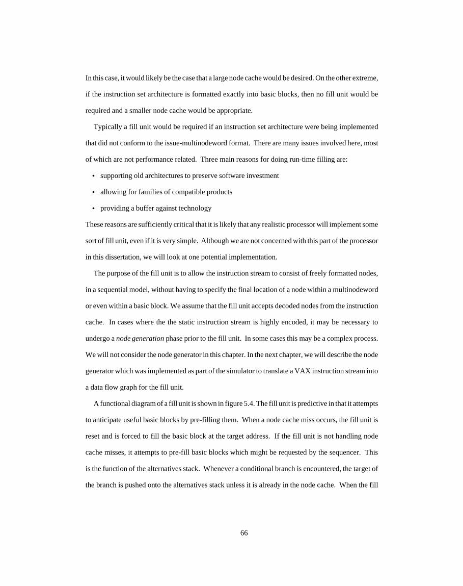
In this case, it would likely be the case that a large node cache would be desired. On the other extreme,

if the instruction set architecture is formatted exactly into basic blocks, then no fill unit would be

required and a smaller node cache would be appropriate.

Typically a fill unit would be required if an instruction set architecture were being implemented

that did not conform to the issue-multinodeword format. There are many issues involved here, most

of which are not performance related. Three main reasons for doing run-time filling are:

• supporting old architectures to preserve software investment

• allowing for families of compatible products

• providing a buffer against technology

These reasons are sufficiently critical that it is likely that any realistic processor will implement some

sort of fill unit, even if it is very simple. Although we are not concerned with this part of the processor

in this dissertation, we will look at one potential implementation.

The purpose of the fill unit is to allow the instruction stream to consist of freely formatted nodes,

in a sequential model, without having to specify the final location of a node within a multinodeword

or even within a basic block. We assume that the fill unit accepts decoded nodes from the instruction

cache. In cases where the the static instruction stream is highly encoded, it may be necessary to

undergo a node generation phase prior to the fill unit. In some cases this may be a complex process.

We will not consider the node generator in this chapter. In the next chapter, we will describe the node

generator which was implemented as part of the simulator to translate a VAX instruction stream into

a data flow graph for the fill unit.

A functional diagram of a fill unit is shown in figure 5.4. The fill unit is predictive in that it attempts

to anticipate useful basic blocks by pre-filling them. When a node cache miss occurs, the fill unit is

reset and is forced to fill the basic block at the target address. If the fill unit is not handling node

cache misses, it attempts to pre-fill basic blocks which might be requested by the sequencer. This

is the function of the alternatives stack. Whenever a conditional branch is encountered, the target of

the branch is pushed onto the alternatives stack unless it is already in the node cache. When the fill

66

unit is free from servicing node cache misses, it pre-fills the address on the top of the alternatives

stack. It is also used when we execute a subroutine call; we simply push the return address. In this

way, there is a good chance that the return basic block will be pre-filled upon a return instruction.

The fill structure consists of a basic block under construction. When a basic block is started, the

fill unit saves the start PC field using the address of the entry point. In addition, the memory pointer

and arithmetic pointers are reset. These pointers are incremented as nodes are filled into the fill

structure. These pointers indicate the last full node within the entry for each of the two types of

nodes.

Figure 5.4Fill Unit Implementation

A A

B status

M A

A pointer

PC #2

Fill Structure

filled basicblocks to node

cache

sequential node stream

address into fill structurevalid bit

BRAT

PC #1

M pointer

Basic BlockEnlargement

Control

AlternativesStack

Start PC

67

For each node processed, the fill unit uses its type (memory or ALU) to determine where to insert

it in the entry. Each operand in a node is either a constant or a register reference. If an operand is a

constant, its value is simply copied into the fill structure. If a node operand is a register reference,

the fill unit uses the BRAT (basic block register alias table) to ensure that dependencies within a

multinodeword and within a basic block are satisfied.

Each entry in the BRAT corresponds to a general purpose register. There are two fields in each

entry: the valid bit and the address field. The valid bit indicates validity of the address field.

Whenever a new basic block is created, all valid bits are reset to signify that no writes have taken

place within that basic block. If an operand reads the value in a register, the BRAT valid bit for that

register is consulted. If the bit is reset, the register reference is left unchanged (at node merge time,

the RAT in the SUNIT will translate the reference). If the valid bit is set, the register reference is

changed into a node reference. This situation indicates that a previously filled instruction has written

to the register. The address field is used as a basic block relative address.

If a node writes to a register, the valid bit is set and the address field is updated with the fill cache

address of that node. If the valid was previously set, the previous contents of the address field are

used to delete the previous register write. This is so that no more than one update to a register will

occur within a single basic block. Note that the fill unit is free to place nodes anywhere within the

fill structure. Register writes are only seen across basic block boundaries. This is accomplished

through the banking of the RAT, described below.

The node cache is responsible for caching basic blocks. Note that the node cache is above the

DSI, thus no dynamic information has been added. We assume that the node cache has a basic block

oriented structure. That is, in addition to the actual issue-multinodewords for a given basic block,

there is also a header which contains the two alternate PCs and a branch status field. Thus, when an

entry point is matched, the header is retrieved to immediately provide information as to the

termination of the basic block. In the case that there is no fill unit the compiler will be responsible

for creating the static instruction stream in this structure.

68

The node cache is indexed based on the architectural PC. In some cases of hardware translation,

it may be necessary to add tags to the architectural PC of a node cache entry for matching. This is

the case for:

• enlarged basic blocks where multiple instances for a single architectural PC exist,

• basic blocks which are too large for a single entry and thus must flow over into a secondentry,

• architectural atomic units which have internal branches and thus require a set of basic blocksfor the same architectural PC,

• certain optimizations where the same architectural PC might have different translationsdepending on the context of the entry.

5.2.2 Basic Block Sequencer

The basic block sequencer contains all logic necessary to sequence the multinodewords being sent

to the SUNIT. This includes branch prediction as well as the logic necessary for backing up the

machine in the case of an exception or a branch prediction miss. The backup procedure allows the

machine to recover from a branch prediction miss and continue without having to drain the pipeline.

Basic blocks are requested from the node cache and issue-multinodewords are fed one at a time to

the SUNIT. The basic block sequencer accepts control signals from assert nodes in the data path and

provides control signals to the data path to control retirement and backup. The distribution bus must

also be monitored. This is necessary to handle computed branches (subroutine returns, case

instructions and dynamic branches) as well as to determine when retirement of a basic block is

possible.

The basic block sequencer contains what we call a window management system. This logic is

responsible for keeping track of what within the machine are currently in progress and where it is

located. The term window is used to refer to the collection of work that is currently being processed.

The window size may be measured in terms of several different things: the number of active basic

blocks, the number of valid nodes, the number of active nodes and the number of ready nodes. A

node may be in any of the following four states:

• empty (an empty node slot, a NOP)

69

• waiting (a node whose operands have not yet been distributed)

• ready (a node ready for scheduling but not yet scheduled)

• fired (a node already scheduled but not yet retired)

In addition, an active node is a node that is waiting or ready and a valid node is one that is waiting

or ready or fired. In a dynamically scheduled processor, a large window size allows parallelism to

be exploited over a large portion of the dynamic instruction stream. In the case of a statically

scheduled processor, there is no window because nodes get merged and scheduled immediately. The

compiler has tried to take advantage of this same sort of parallelism by scheduling nodes within node

slots statically.

In the case of a statically scheduled machine without enlarged basic blocks, the only need for

backup is to allow memory exceptions to be precise. Our model does not implement branch

prediction for statically scheduled machines, so there is no branch prediction miss backup. This is

because in the case of static scheduling, the only benefits of branch prediction are to allow

pre-fetching of the instruction stream (which is not measured) and to save potentially one delay slot

in merging. This latter effect complicates the scheduling of register results across branches and in

any case is an effect which is easily computable.

Backup in the case of dynamic scheduling is much more critical and this is where window

management comes in. The dynamically scheduled processor is designed to allow the merger to

continue across branches and allow efficient recovery in the case of branch prediction misses. Usually

when a basic block is started, two explicit locations for the next basic block are available. A

prediction is made and one of the two basic blocks will be merged when the current basic block is

done. This procedure continues until either a signal is received from the execution unit or memory

unit or a resource conflict occurs. A resource conflict can either be a limitation on the number of

active basic blocks allowed (since backup information must be saved for each dynamic basic block

boundary) or a limitation on the size of the node tables in the execution or memory units.

70

When a signal is received from an assert node, it is classified as either a trap or a fault and after a

backup operation will either cause merging to stall or will initiate merging down another path. In

the case of memory fault (e.g. an address range fault) the window management system will backup

to the point before the basic block containing the errant node and will stall. There are certain types

of basic blocks which have a termination condition which automatically causes a stall. These are

basic blocks which end with system calls. After all basic blocks have been retired, the system request

is made. System calls are treated as synchronization points and thus all work is retired, but in practice

this is not absolutely necessary. However, explicit synchronization is necessary in cases of multi-

processor communication and I/O. We assume that I/O and shared memory is explicitly handled by

basic block synchronizers and thus no checking for special memory addresses within the memory

unit is performed. The order of memory reads is not guaranteed, even across branches, thus they

cannot have side-effects or be allowed to change externally.

Any resource which can be modified by non-confirmed nodes must be protected since backup

may be necessary. All registers (via the RAT and SPAT), node table entries, and write buffer entries

are protected. The node tables and SPAT have one bank for each active basic block while the RAT

and the write buffer have one more than this number. Some other miscellaneous registers, including

branch prediction histories are also protected since they can be modified. The extra RAT and write

buffer bank are used to store the consistent state of the machine. The machine can always back up

to the consistent state. Associated with each bank is a PC address which corresponds to the instruction

stream location which began the bank. Basic block retirement is possible when all prior basic blocks

have retired, all nodes merged within the basic block have executed and all write buffer entries in

the consistent state bank have been flushed

Signals from the data path to the basic block sequencer include arithmetic exceptions and assertion

failures. An assertion failure occurs when an assert node which was generated to detect an assumed

condition determines that the assumed condition does not apply. Assert node are used for branch

prediction confirmation, but they may also be used for other purposes. The idea would be to treat

71

rare conditions as though they were exceptions. Array bounds checking is a prime example. By using

assert nodes to verify array bounds, we can optimize for the common case and minimize the time we

have to spend processing control instructions.

5.3 Scheduling Unit

The scheduling unit (SUNIT) consists of the RAT, the SPAT and the node tables. The alias tables

are responsible for enforcing all flow dependencies while removing all anti and output dependencies.

The merging process consists of accessing the alias tables and modifying the nodes as the are sent

to the node tables. The node table and associated scheduling logic hold the nodes after they have

been merged and determine when they can be sent to the function units.

5.3.1 Register Alias Tables

A block diagram of the merging process performed by the SUNIT is shown in figure 5.5. Both

the RAT and the SPAT monitor the distribution buses. The RAT has one entry for each of the

architecturally visible general purpose registers. Each entry either contains a value or a tag for a

node which is yet to be distributed. A ready bit indicates whether the value field is valid or not. The

SPAT is needed to handle references to other nodes within a basic block. The merging process for

a single basic block may take many cycles. Thus it cannot be guaranteed that a node result used later

in the same basic block will not already have been distributed when the node that uses it is merged.

The SPAT catches nodes being distributed for the basic block being merged only. When a node

operand refers to a previous node, the SPAT is consulted to determine if the reference should be

converted to a literal or to a global node tag.

In order to handle backup, each entry in the RAT (i.e., each architectural general purpose register)

is organized as shown in figure 5.6. This is an example for four banks, some other number may

actually be implemented. For each architecturally defined general purpose register, there are five

physical registers. Four registers include logic to monitor the distribution buses. The fifth register

is used for storing values only; it represents the save state of the architectural register. In addition,

72

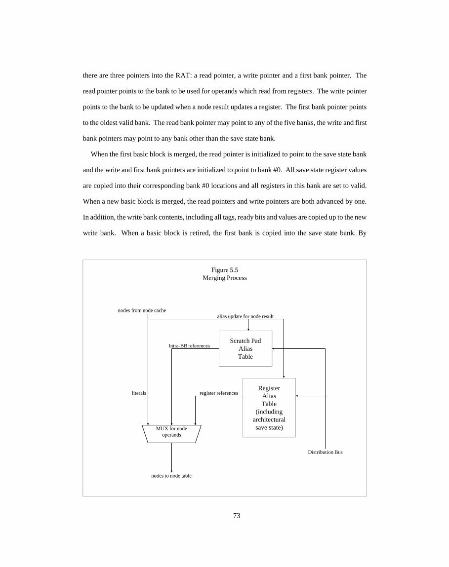
there are three pointers into the RAT: a read pointer, a write pointer and a first bank pointer. The

read pointer points to the bank to be used for operands which read from registers. The write pointer

points to the bank to be updated when a node result updates a register. The first bank pointer points

to the oldest valid bank. The read bank pointer may point to any of the five banks, the write and first

bank pointers may point to any bank other than the save state bank.

When the first basic block is merged, the read pointer is initialized to point to the save state bank

and the write and first bank pointers are initialized to point to bank #0. All save state register values

are copied into their corresponding bank #0 locations and all registers in this bank are set to valid.

When a new basic block is merged, the read pointers and write pointers are both advanced by one.

In addition, the write bank contents, including all tags, ready bits and values are copied up to the new

write bank. When a basic block is retired, the first bank is copied into the save state bank. By

RegisterAliasTable

(includingarchitecturalsave state)

Scratch PadAliasTable

Figure 5.5Merging Process

Intra-BB references

register referencesliterals

nodes to node table

Distribution Bus

nodes from node cachealias update for node result

MUX for nodeoperands

73

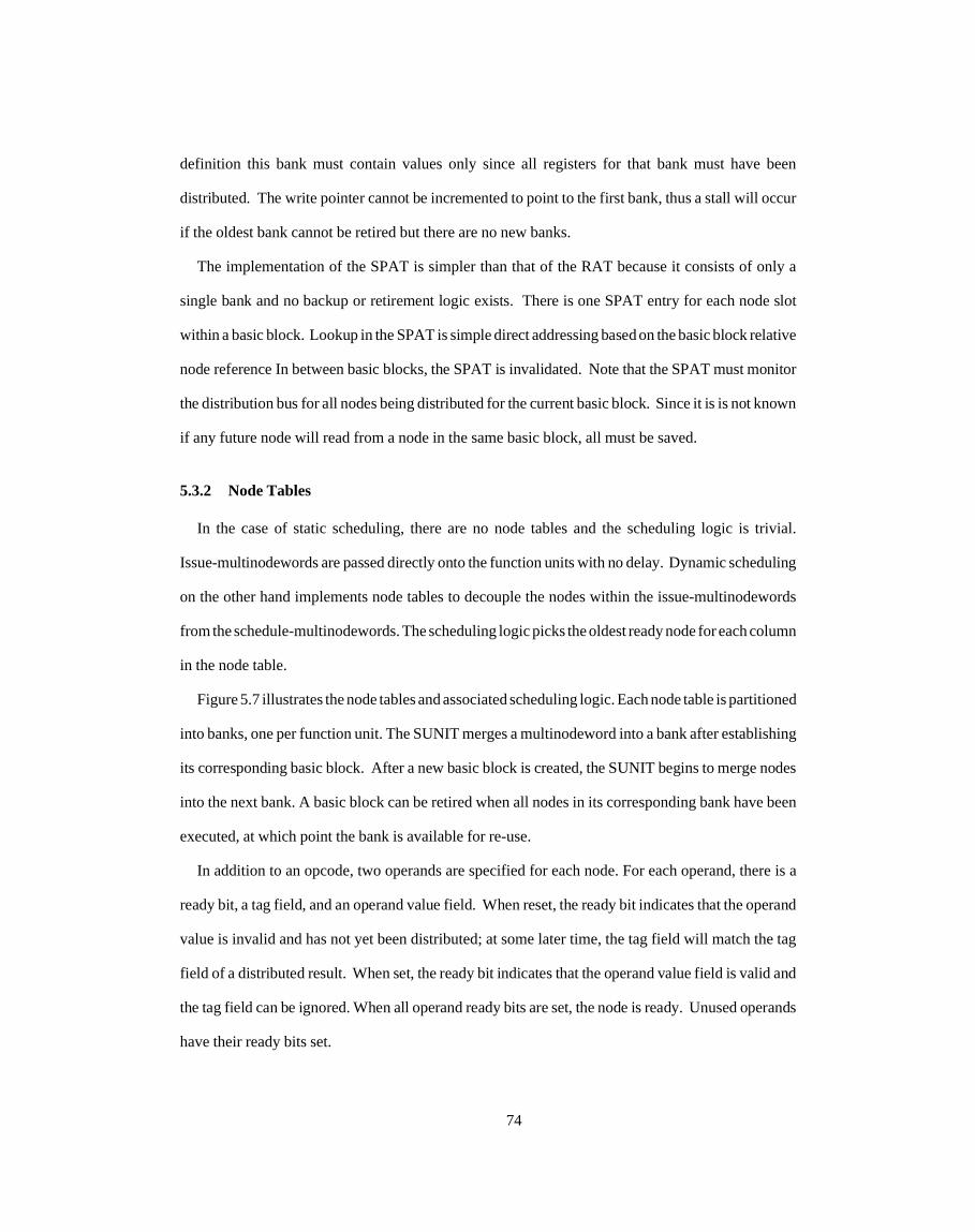
definition this bank must contain values only since all registers for that bank must have been

distributed. The write pointer cannot be incremented to point to the first bank, thus a stall will occur

if the oldest bank cannot be retired but there are no new banks.

The implementation of the SPAT is simpler than that of the RAT because it consists of only a

single bank and no backup or retirement logic exists. There is one SPAT entry for each node slot

within a basic block. Lookup in the SPAT is simple direct addressing based on the basic block relative

node reference In between basic blocks, the SPAT is invalidated. Note that the SPAT must monitor

the distribution bus for all nodes being distributed for the current basic block. Since it is is not known

if any future node will read from a node in the same basic block, all must be saved.

5.3.2 Node Tables

In the case of static scheduling, there are no node tables and the scheduling logic is trivial.

Issue-multinodewords are passed directly onto the function units with no delay. Dynamic scheduling

on the other hand implements node tables to decouple the nodes within the issue-multinodewords

from the schedule-multinodewords. The scheduling logic picks the oldest ready node for each column

in the node table.

Figure 5.7 illustrates the node tables and associated scheduling logic. Each node table is partitioned

into banks, one per function unit. The SUNIT merges a multinodeword into a bank after establishing

its corresponding basic block. After a new basic block is created, the SUNIT begins to merge nodes

into the next bank. A basic block can be retired when all nodes in its corresponding bank have been

executed, at which point the bank is available for re-use.

In addition to an opcode, two operands are specified for each node. For each operand, there is a

ready bit, a tag field, and an operand value field. When reset, the ready bit indicates that the operand

value is invalid and has not yet been distributed; at some later time, the tag field will match the tag

field of a distributed result. When set, the ready bit indicates that the operand value field is valid and

the tag field can be ignored. When all operand ready bits are set, the node is ready. Unused operands

have their ready bits set.

74

While most nodes are either monadic or dyadic, nodes of higher degree are supported through the

use of a special opcode bit. When an entry with this bit set is scheduled, the next sequential entry in

the node table is delivered to the execution unit in the subsequent schedule phase. This allows the

convenient handling of nodes with 64-bit inputs and 64-bit outputs (e.g. extended precision floating

point). If an entry has this extended bit set in the opcode field, the scheduling logic can consider it

Figure 5.6Register Alias Table Detail

RAT Bank #0(tags and values)

RAT Bank #1(tags and values)

RAT Bank #2(tags and values)

RAT Bank #3(tags and values)

Architectural Save State(values only)

local bus (for bank advancement,retirement and backup)

Distribution Bus

mergewritebus

mergeread bus

write pointer

first bank pointer

read pointer

75

ready only if the next sequential entry also has both operands ready. Node extension entries have

their valid bits reset to prevent them from being treated as separate entries by the scheduling logic.

Each node table monitors all results distributed in a distribution cycle. The tag of each operand

is compared with the tags on all the distribution buses. If an operand ready bit is reset, a tag match

will cause the ready bit to be set and the distribution bus value to be latched.

In merging, nodes are stored in the bank corresponding to the current checkpoint and a current

available pointer (which points to the next place in the bank to merge a new node) is incremented.

Note that if an extended node is to be merged, the extension entry must be merged non-valid in one

cycle, and the primary node must be merged valid in the next cycle. This is necessary to avoid a

possible scheduling race condition.

5.3.3 Memory Node Tables

Unlike the arithmetic node tables, the memory node table must resolve dependencies between

nodes. The arithmetic node tables do not have to resolve these dependencies because the SUNIT

does this at merge time. The alias tables can determine dependencies between all nodes that operate

on registers because register numbers are always known from the instruction stream (we do not allow

indirect references to registers). The alias tables cannot, however, determine dependencies between

memory operations because the addresses are generally not known at merge time. Thus, the memory

node table must have logic for resolving memory dependencies in addition to the distribution and

merge logic present in the other node tables. This dependency resolution logic, which incorporates

memory address disambiguation hardware, is non-trivial. Two problems, unknown addresses and

partial dependencies make the implementation difficult. Another feature that complicates the

memory node tables is the implementation of multiple memory nodes per cycle.

Unaligned accesses are not allowed. Thus, all data accesses of 1, 2, or 4 bytes will always be

contained in a single aligned 32-bit word. Each memory node contains a 4-bit mask indicating which

of the four bytes are part of the associated access. The low two bits of the memory address along

with the size of the access are used to set these bits.

76

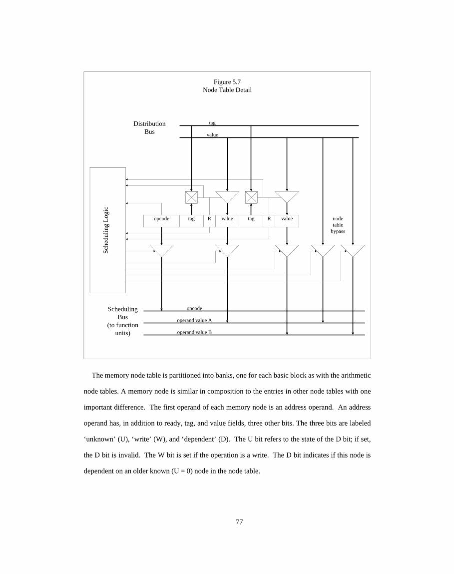
The memory node table is partitioned into banks, one for each basic block as with the arithmetic

node tables. A memory node is similar in composition to the entries in other node tables with one

important difference. The first operand of each memory node is an address operand. An address

operand has, in addition to ready, tag, and value fields, three other bits. The three bits are labeled

‘unknown’ (U), ‘write’ (W), and ‘dependent’ (D). The U bit refers to the state of the D bit; if set,

the D bit is invalid. The W bit is set if the operation is a write. The D bit indicates if this node is

dependent on an older known (U = 0) node in the node table.

tagopcode R tag valueRvalue

Sche

dulin

g L

ogic

Figure 5.7Node Table Detail

DistributionBus value

operand value A

SchedulingBus

(to functionunits)

tag

operand value B

opcode

nodetable

bypass

77

Memory nodes are merged unknown (U = 1), regardless of whether the address operand is ready.

This simplifies merge logic, as D bits do not have to be generated at merge time. An address operand

will be merged ready if the address is known at merge time (either immediate in the instruction stream

or in a valid register). The W bit is set if the operation is a write and reset if it is a read. The process

of merging a memory node does not affect any other nodes in the node table. During distribution

ready bits are set for operands that are being distributed.

The node table performs D bit generation. This involves choosing the oldest node with the U and

R bits both set. This node is then enabled to gate its address onto an internal bus. This information

is then used in two ways. Younger nodes use this information to decide if they are dependent and

set their D bit correspondingly. Also, the node that was selected uses information from older nodes

to decide if it is dependent and sets its own D bit correspondingly.

The operation is as follows. For the selected node, the D bit is set if and only if there exists an

older node which overlaps this node. (In the case of read nodes, only write node overlaps are

significant while in the case of write nodes, any overlap is significant.) For each younger memory

node (with respect to the selected node), if there is an overlap with the merged node, the D bit for

the younger node are set in a similar manner. This operation ensures that younger memory nodes are

properly set dependent according to this memory node and the selected node will be set properly

dependent on any older memory node. We do not care about unknown address nodes that are older,

as they properly inhibit scheduling. At the end of the D bit generation cycle, the U bit for the selected

node is cleared.

Execution selection and scheduling then take place. This involves choosing the oldest node with

the conditions that: (1) U = 0, D = 0, (2) the other operand is ready, and (3) no older nodes exist with

U = 1. (To be more precise, read nodes can’t fire if there exist any older write nodes with U = 1 while

write nodes can’t fire if there exist any older read or write nodes with U = 1.) If there exists such a

node, it is delivered to the write buffer and virtual cache. Execution of this node might mean that

78

previously dependent younger nodes are no longer blocked from execution. Thus, during scheduling

the D bit for all nodes younger than the node selected for execution must be updated.

This mechanism operates as follows. Any node with U = 0 that is younger than the node being

scheduled resets its D bit if and only if it is the oldest node that overlaps. Actually, the logic is a bit

more complex. If the node being scheduled is a read node, only write nodes are allowed to clear their

D bits since read nodes never set their D bits due to another read node. If the node being scheduled

is a write node, however, both read and write nodes take part but in different ways. An overlapping

read node will prevent younger overlapping write nodes from clearing their D bits but will not prevent

younger overlapping read nodes from doing so. But, overlapping write nodes will prevent all younger

overlapping nodes from clearing their D bits.

Now consider the implementation of multiple memory node tables. The memory system is

composed into banks based on the low bits of the 32-bit access. Each memory node table gets all

the memory nodes within the issue-multinodeword. As addresses are resolved, any node which does

not contain the appropriate address bits for that node table is simply invalidated. All of the

dependency detection hardware is implemented as above for each node table. In the case of static

scheduling, we look at each node within the multinodeword and allow them to proceed if there are

no bank conflicts. Bank conflicts will cause single cycle stalls in the pipeline.

5.4 Execution Unit

The EUNIT contains the ALUs as well as all queueing logic for the distribution buses. An

overview of the a single ALU is shown in figure 5.8. The function units are connected to distribution

buses which return results to the SUNIT. Each function unit which is scheduled to actually consists

of several function units which vary in pipeline depth. In an actual machine, it would probably make

sense to have a smaller number of complex function units with input queues from the main function

units. The idea being that certain complex function units execute functions that are not common

enough to replicate. The scheduling logic connected to each node table using the opcode could either

79

route it to the simple function unit or to the appropriate complex function unit. Thus, nodes forwarded

to them for execution may have to be queued.

When a node is sent to a complex function unit, it sends along a tag indicating which of the three

node tables it came from. Then, when the result is generated, it will distribute on the bus associated

with that node table. This keeps the distribution buses balanced. Note that complex function units

prevent the associated simple function unit from distributing in that cycle (since the complex function

unit node is older). Thus, simple function unit results may have to be queued also. When either the

complex function unit input queue or the simple function unit output queue for a particular node table

is full, the scheduling logic associated with that node table will stall.

Simple function units can complete their operation in one cycle. The functions implemented are

standard 32-bit ALU operations as well as some special purpose operations. Functions implemented

in the simple function units are those that are either executed frequently or are inexpensive to

duplicate. Each function unit takes two 36 bit input operands (a 32 bit value plus four condition code

bits) and produces a 36 bit result.

The complex function units implement operations that are not common enough to replicate.

Unlike the simple function units, they may take any number of cycles to complete. They may be fully

pipelined (allowing them to take a new operation every cycle), partially pipelined or not pipelined

at all. There also may be more than one function unit that implements the same operation.

5.5 Memory Unit

Figure 5.9 provides an overview of the memory unit (MUNIT), which processes nodes related to

the memory system forms the interface to main memory. Memory nodes are merged into the memory

node table in the SUNIT. After resolving any dependencies, nodes are then routed to the virtual cache

(in the case of reads) and to the write buffer. After a basic block retires, the consistent write buffer

bank is written to the virtual and physical caches.

Another feature of the MUNIT is a write-through virtual cache. The virtual cache is connected to

a larger physical cache after translation through a TB. The write buffer also interacts with the TB

80

to obtain translation information when a write node fires. This is necessary to guarantee completion

of write nodes after the corresponding basic block has retired.

The memory write buffer is provided to handle backup of memory nodes. Recall that in order to

handle backups to the general register set, the RAT is split into several banks, each of which is

dedicated to one basic block. When backup is necessary, all that is needed is that we discard all bad

RAT banks created after the basic block. However, this will not work for memory nodes because we

cannot contain the entire state of the memory system in the machine. Thus, we must use some other

method for allowing backup of write nodes.

One option is the so called ‘optimistic memory unit’ design approach described in Wen-mei Hwu’s

Ph.D dissertation [Hwu87]. He suggests that backup of memory is seldom needed and, when it does

occur, very little actually needs to be backed up. To implement a recovery system, a write node reads

the previous value of the memory location before it actually writes. This previous value is then saved

in the checkpoint, and, in the event recovery is necessary, the saved values are re-written to their

proper places.

A difficulty with this scheme is that at the time of the backup, we are forced to individually replace

saved values, which would necessarily lengthen the branch prediction repair time which is important

to minimize due to the high branch density. Also, in a multiprocessor system writing through and

possibly updating other processors and later writing back the correct value would complicate

synchronization between processors.

Here we propose an alternative scheme which is the use of a write buffer. A write buffer saves

written values associated with a basic block until the basic block is retired. At that time, all values

stored in the write buffer are written back to the memory system. The write buffer is actually a small

fully associative write-back cache. For any read node, the write buffer is accessed in parallel with

the virtual cache access. If a match occurs in the write buffer, that data is distributed.

The write back is done after basic block retirement time. The write buffer is constructed to only

contain 32-bit aligned writes. One advantage of the write buffer scheme is fast backup. If we need

81

to back up, we simply flush the write buffer banks associated with invalid basic blocks. Another

advantage of the scheme is its ability to correctly update other processors (in a multiprocessor

environment) since writes do not occur until a checkpoint is retired (implying that no fault has

occurred).

Figure 5.8Function Unit Overview

not fullyreplicatedfunctions

fullyreplicatedand fullypipelinedfunctions

fullyreplicated

but not fullypipelinedfunctions

Distribution Bus

opcode andoperands from node table

from other node tables

82

Each entry in the write buffer is fully associative. In the event of a partial write to a word (i.e. a

8-bit or 16-bit access), the full word is fetched before the entry is made in the write buffer. Each entry

consists of a valid bit, a dirty bit, a virtual address tag, a physical page number and 32 bits of data.

Write nodes are considered executed when they have updated the write buffer. This process involves

accessing the translation buffer to obtain the physical page number in addition to the possible read

in the case of a partial word write. After checkpoint retirement time, each dirty entry is written back

to the virtual cache and the physical cache and is then invalidated. When all entries in the consistent

state write buffer bank are invalidated, the next checkpoint is allowed to retire.

Figure 5.9MUNIT Overview

backup and retirementcontrol from IUNIT

nodes from memorynode table

to main memory andI/O system

Distribution Bus

VirtualAddress Cache(write through)

TranslationBuffer

Physical AddressCache

(write back)

WriteBuffer

instruction-stream to IUNIT

83

Chapter 6 Simulation Description and Results

In this chapter we describe the simulation study which was conducted and present the results from

that study. The abstract processor model described in the previous chapter provides the foundation

of the simulation study. Data was collected under a variety of machine configurations for a variety

of benchmarks. Here we focus on that data collection process and the analysis of the results.

This chapter is divided into three sections. In the first section we provide an overview of the

simulator. The second section presents the experimental methodology, outlining the parameteriza-

tion of the abstract processor model and indicating the choice of benchmarks. In section three we

present the results.

6.1 Simulator Overview

An overview of the simulation process is shown in figure 6.1. There are two basic components:

the translating loader (tld) and the run time simulator (sim). The translating loader does an object

code to object code translation from a VAX executable file to a file of fully decoded multinodewords.

The run time simulator reads in the translated code and does a cycle by cycle simulation of the

program. System calls that are embedded in the original program are executed by the operating

system on which the simulator is running. The run-time simulator collects statistics on the execution

of the entire program except for the system calls themselves; thus, it represents the user level or

unprivileged portion of the execution.

The configuration parameter which is passed to the two parts of the simulator indicates the machine

configuration for which the data is to be collected. Not all distinct configurations require distinct

translated files. In particular, the window size for dynamic scheduling is not reflected in the translated

file, it is processed by the run-time simulator only. The memory model also does not affect the

translated file except in the case of static scheduling, where the target memory latency is needed.

Both the translating loader and the run-time simulator collect data in a specified statistics file.

84

The creation of a basic block enlargement file is handled by a separate program, ‘‘mkbbfile,’’

which uses the statistics file. It combines basic blocks with high frequency branches between them

into extended basic blocks. In the case of loops, multiple iterations are unrolled. The basic block

enlargement file may then be used as input to the translating loader. The run-time simulator also

supports static branch prediction (used to supplement the dynamic branch prediction) and a trace

mode that allows the simulation of perfect branch prediction.

The division of the simulator into two pieces was done for convenience in data collection. The

translating loader stores the programs fully decoded, but it is not expected that an actual machine

VAX/BSDObject Code File

TLDTranslating

Loader

TranslatedProgram File

SIMRun-timeSimulator

MeasurementData File

MKBBFILE

Branch TraceFile

Static BranchPrediction File

Basic BlockEnlargement File

Input Data

MachineConfiguration

Figure 6.1Simulation Process Overview

85

would be designed for such an instruction stream. For a small price in run-time decoding, the

instruction bandwidth could be significantly reduced. Also, in the case of a dynamically scheduled

processor, a more general format to be passed through a fill unit would obviate having the compiler

know the exact function unit configuration. In this section we will first describe the translating loader,

then the run-time simulator.

6.1.1 Translating Loader

An overview of the translating loader is shown in figure 6.2, it consists of approximately 9700

lines of C. There are two main pieces, the node generator and the fill unit. The translation process

takes place for the entire program before program execution. Therefore, it is technically below the

above the DSI, even though in an actual processor it may be below the DSI. (Recall from chapter 3

that we distinguish translation activities above the DSI from those below the DSI by whether or not

a new representation of the program is created separate from the internal state of the processor.)

The translating loader is a two pass translator. A temporary file and an address map are created

on the first pass. The second pass translates all old code space addresses to new code space addresses.

This remapping is needed in three cases: branch destinations, literal PC values and jump tables entries.

Literal PC values arise in PC pushes for subroutine calls, nodes which compute jump table indices

and for branch fault nodes (used for basic block enlargement). The second pass also appends the

initialized data from the original object code to the translated file.

The mapping structure maps for each new PC, three pieces of information: the corresponding old

PC, the context and the instance number (see figure 6.3). The context of a generated basic block

consists of two groups of information: call context and register context. The call context is the current

argument count and register save mask. It is used for call/return optimization discussed below. The

register context is the current distribution slot for each of the architectural registers. It is used only

in the case of static scheduling to allow register results to be forwarded across branches.

When we use the term entry point, we mean an old PC, context pair. The third piece of information

in the mapping structure is the instance number. This is used for basic block enlargement. It

86

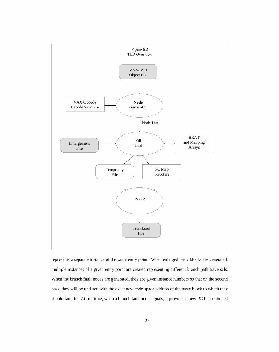
represents a separate instance of the same entry point. When enlarged basic blocks are generated,

multiple instances of a given entry point are created representing different branch path traversals.

When the branch fault nodes are generated, they are given instance numbers so that on the second

pass, they will be updated with the exact new code space address of the basic block to which they

should fault to. At run-time, when a branch fault node signals, it provides a new PC for continued

VAX/BSDObject File

NodeGenerator

FillUnit

Node List

TemporaryFile

Pass 2

TranslatedFile

BRATand Mapping

ArraysEnlargement

File

VAX OpcodeDecode Structure

PC MapStructure

Figure 6.2TLD Overview

87

execution. The basic block generated with an instance number of zero for a given entry point is the

default basic block, it will be executed first. In the remainder of this section we will discuss details

of the node generator and the fill unit.

6.1.1.1 Node Generator

The node generator can be thought of as reversing the code generation phase of the compiler and

applying optimizations. The VAX object code is used as input and a directed acyclic graph is

produced. The node generator operates on the instruction stream one VAX instruction at a time and

generates for each instruction a list of nodes. This list is in what we call sequential correct order,

which means that correctness is preserved if they are executed in the order given. This implies two

restrictions:

• nodes cannot use as inputs the output from later nodes

• updates to registers are interpreted sequentially

Due to the differing models involved, the production of a sequential correct order is not as simple

as it might seem. The VAX Architecture is specified with a microprogrammed state machine in

mind which interprets the instruction stream as it is executed. The node generator needs to produce

a static data flow graph, suitable for execution at a later time.

A fundamental problem in converting between these two paradigms occurs in the processing of

operands with side-effects. According to the VAX architecture, operands are interpreted in instruc-

New PC(address into

translated file)

Old PC (address into original file) Context Call Context Register Context

Instance Number

EntryPoint

1 - 1Correspondence

Figure 6.3Mapping Structure

88

tion-stream order and side-effects are processed one at a time. This in itself is not so much of a

problem, it just requires the decoding of the instruction stream and the generation of the nodes in

instruction-stream order. The main problem is that operand values (in the case of read and modify

access types) and operand addresses (in the case of modify, write and address access types) are

supposedly saved during operand processing. When operand addresses are generated rather than

coming from a register (i.e. they are the result of a read or an ALU operation), there is no problem

because the address is implicitly saved by the fact that the node generates a new result. However,

when operands or operand addresses are coming directly from registers, the node generator would

rather leave them there until it generates the nodes which will use them. The alternative is to generate

a redundant move node to save the contents of the register.

The goal was to generate a sequential-correct node order with an insignificant number of redundant

move nodes, and in practice this was achieved. In some cases redundant nodes are unavoidable but

those cases are mainly pathological. A simple example of when a redundant move would be

necessary (although not present in the VAX architecture) would be an instruction which swaps two

registers, for example:

SWAP R0, R1

This instruction would have to generate three move nodes in order to create a sequential correct

order. In the case of static scheduling, this extra move node (the first one generated) will write to a

temporary register and the third move node will read from that register. In the case of dynamic

scheduling, the extra node will not specify a named register, the third move node will just refer to

the first node directly. The reason this a redundant node is that it could be eliminated if the node

generator could guarantee that the other two nodes would end up in the same issue-multinodeword.

In the case of a dynamically scheduled processor, it is only necessary that the two move nodes be in

the same execution atomic unit.

In practice, situations like this where the node generator produces less than optimal sequences in

order to preserve generality are very rare. The generation of nodes from VAX instructions has been

89

highly optimized to remove as many architectural dependencies as possible and produce the

minimum number of nodes in almost all instances. In several cases this involved placing restrictions

on the object code. These restrictions did not prove to be serious limitations. The most significant

ones are described below. It should be pointed out that these don’t represent limitations of the abstract

processor model, but limitations of TLD to simplify the translation process. An actual processor

with its own compiler could overcome these restrictions.

Dynamic Branches. The use of dynamic branches, such as: JSB (R0) and CALLS $0, *funcptr

is not permitted. The reason for this is twofold. First, without knowing all possible destinations of

the branch statically, it is not possible to guarantee that all possible entry points have actually been

generated. Second, without knowing how the address was generated, it cannot be guaranteed that

adjustments have been made for the code space relocation. The only instance of a run-time generated

address that is supported is a branch through a memory read node. There are three instances of this:

RSB, RET, and CASE. The return instructions will only work if the addresses being read correspond

to previously executed JSB or CALL instructions, and if the address has not been modified on the

stack.

Instruction Stream Literals. CASE instructions must have limit operands which are instruction

stream literals. This allows the translating loader to interpret the jump table and translate code for

all entry points. PUSHR and POPR instructions most have the mask operand as an literal so the

actual register operations may be generated. CHMK instructions (system calls) must have the code

operand as a literal.

Variable Bit Field Instructions. For all 13 of these instructions (BBx, CMPV, EXTV, FFx,

INSV) two restrictions apply. The base address must be aligned to a four byte boundary and the field

itself may not cross a four byte boundary (or a register boundary for register operands).

An example of optimization that deserves special mention is the handling of VAX procedure calls

and returns. These instructions have been heavily modified, discarding all but the essential parts of

the call frame. This will work only so long as CALLx / RET sequences are generally well behaved

90

and no code tries to access the call frame directly. As pointed out above, the destination (and thus

the register save mask) must be known statically. This permits the generation of explicit register

save and restore nodes. When a return is encountered, the appropriate register save mask is used.

During the static analysis of the program, the call context is saved at each branch so this will work

correctly even for recursion or if two entry points with different masks return through the same return

instruction. However, it will not work if masks are accessed on the stack and in cases where a return

does not match a call (e.g. if the call mask is constructed on the stack before the return).

The other optimizations to the procedure call are the following: the stack is assumed to be aligned,

the PSW is not preserved and the condition handler 0 is not written (this optimization saves two

32-bit writes to the stack). The FP points to the saved AP in the stack frame. In the case of CALLS,

the numarg argument is not placed on the stack, it is part of the call context which is processed during

node generation. When the return is encountered, an explicit adjustment to the stack is made. This

optimization saves an additional 32-bit write to the stack. In the case that the same procedure is

called with differing numbers of arguments, two different versions of the return sequence will be

generated.

6.1.1.2 Fill Unit

The fill unit is responsible for taking node lists produced by the node generator and scheduling

the nodes into multinodewords. It can generate code for both dynamic and static scheduling. If static

scheduling has been selected, the nodes will be placed into a basic block structure such that

intermediate results will be forwarded properly, assuming the multinodewords are scheduled in the

order created. The ALU function units have known latencies that are always met while memory is

assigned a predicted latency which is guaranteed by the hardware. Nodes which need results from

other nodes are placed in a multinodeword slot far enough back to ensure that the value will be ready.

Distributed results may either go directly to the input of a function unit (a pipeline bypass) or to the

register file. If the case of a pipeline bypass, a special tag is placed on the appropriate input and no

91

temporary register is named. For intermediate results which are further away, the fill unit allocates

named temporary registers to hold them.

If dynamic scheduling has been selected, the forwarding of intermediate results is achieved by

chaining node tags together, not based on the physical placement of the nodes within the basic block

structure. The hardware guarantees synchronization of all operands and there are no constraints on

the merge sequencing of nodes. Distributed results go to the node table and to the register file. In

the dynamically scheduled case, we also allow the node table to be bypassed, but only in the case

that there are no older ready nodes to be scheduled.

The fill unit applies most standard optimizations to the code generated. Literals are propagated

through address computation nodes, common sub-expressions are eliminated and ‘orphan’ nodes are

deleted. An orphan node is a node which is no longer chained to any other node in the basic block.

This occurs when the register update of a node is eliminated due to another node writing to the register.

This is common for nodes which generate condition codes which are never actually used. It can also

happen when a literal is propagated and the intermediate value was not needed. Note that in the case

of basic block enlargement, these optimizations are taking place across multiple conditional branches.

This is one of the keys to the advantages of enlarged basic blocks as we pointed out in chapter 4.

When basic block enlargement is specified, the fill unit uses the information from an enlargement

specification file. This consists of instructions as to how many instances and which ones to create

for each old PC. If there are several entry points for a given old PC then several groups of instances

must be created. The basic procedure operates as follows. When the fill unit gets to the end of an

architectural basic block, it checks to see if enlargement is currently active. If so, it will convert the

branch assert node at the end of the basic block from a trap node to a fault node, assign an instance

number to the fault node and continue down one of the branch paths. At the end of the enlarged basic

block, the translated code is output to the temporary file and the next instance is produced. This

procedure has the characteristic that the nodes for an instruction may potentially be re-generated

92

many times. Optimizations could certainly be made to save some duplicated effort but it was not

critical for our purposes.

There are several limitations to the optimizations of the fill unit. First, it employs greedy

scheduling. When a node is first encountered from the node generator, it is placed in the best available

slot at that time and it is not repositioned. This is more of a disadvantage for static scheduling than

for dynamic scheduling. For this reason, the fill unit tends not to be very good at filling branch delay

slots at the end of the basic block. In some cases a re-ordering of nodes within the basic block would

allow the branch node to be placed further ahead and thus eliminate an empty branch delay slot. This

effect is more pronounced for narrow multinodewords than for wide ones. Note, however, that the

effect of not filling a branch delay slot is small and calculable. It could only affect those cases where

an empty slot occurs at the end of a basic block (we measure how often this happens) and it could

only decrease run time by one cycle per instance (since branch confirmation nodes have a latency of

1 cycle).

The second main limitation of the fill unit is that it makes no attempt at static memory disambig-

uation. All memory nodes (except those that may have been deleted due to common sub-expression

elimination or orphan creation) are placed into the basic block in instruction stream order. A more

sophisticated compiler could look at the addresses being generated, even in cases where they are not

statically known, and make optimizations based on them. It could reorder memory accesses when

conflicts are known to occur and it could potentially do a better job of eliminating redundant loads

and stores. For example, suppose a loop variable is kept in memory rather than in a register and this

loop has been ‘enlarged’ through multiple iterations. The intermediate reads and writes as well as

all address computation nodes (if any) should be eliminated and the result should forward directly

within the basic block.

6.1.2 Run-time Simulator

An overview of the run-time simulator is shown in figure 6.4. It consists of approximately 8100

lines of C code. (Of these, approximately 1200 lines are in modules shared with TLD, and there are,

93

BasicBlock

Sequencer

Merger Output Register

RAT

current tags

UNIX4.3 BSD

OperatingSystem

systemcalls

UserInterface User

ProgramArray

I-StreamFetches

DataArray

StackArray

AddressTranslator

Scheduling andExecutionRoutines

Function UnitPipelineRegisters

Distribution Reg.

Memory ReadPipelineRegisters

Distribution Reg.

NodeTables

MemoryWriteBuffer

Figure 6.4SIM Overview

dynamicallyallocatedmemory

94

separate from both SIM and TLD, approximately 2500 additional lines of utility code.) The run-time

simulator does a cycle by cycle simulation for a specified machine configuration of the abstract

processor model (as described in chapter 5). There is no run-time decoding, the fully decoded

program is read in from an external file. The run-time simulator is mainly intended for batch use,

but a command interpreter is present to assist in debugging. It allows the printing of certain

information to be enabled and disabled. After the simulated program terminates (by executing an

EXIT system call), the simulator terminates and statistics gathered during execution are output.

The environment of the simulated program is reproduced by the simulator so as to be just as it

would have been if the original program had been executed. There are three main areas where special

attention was required: command line arguments, address translation and system calls. All of the

benchmarks used in this study take their input operands on the command line. Thus, it was necessary

to prepare a simulated argument list to the program. This was accomplished by using the tail of the

command line to the run-time simulator. The command line is of the format:

sim [options] <program file name> [simulated argument list]

After the options are processed, the remainder of the command line is used to prepare an argument

list on the simulated stack. Then, the argc and argv arguments are created and execution begins at

the first basic block in the file (the envp argument is set to 0).

Address translation is another important feature of the run-time simulator. Recall from chapter 5

that the abstract processor model has separate code and data address spaces. When the run-time

simulator starts up, it allocates a program memory array to hold the translated code. This array can

be read by the sequencer only and cannot be written. No translation is needed for instruction stream

fetches, only an index into the program array. The simulator also creates two more data regions: a

data area, which is the size of the initialized and uninitialized data from the translated file and a stack

area, which is a pre-determined size. All three of these memory regions reside in the data space of

the simulator but the stack grows down from the top of the stack region.

95

When the simulated program requests more memory, through a BREAK system call, this memory

is dynamically allocated on top of the simulator’s data space. One problem is that the simulator itself

also dynamically requests memory after the initial allocation (not explicitly but through the use of

file I/O libraries). It cannot be guaranteed that the new memory requested by the simulated program

is contiguous with the originally allocated data area as it would be if the program were actually

running. Therefore, a mapping structure is used to keep track of the correspondence between the

simulated address space and the simulator address space for all of the memory that has been

dynamically allocated. Data memory accesses can thus be broken into three categories:

• 1. address > 0x3FFFFFFF index into stack array

• 2. address < data array size index into data array

• 3. address >= data array size consult mapping structure for base address of allocated region

If an address range violation is encountered, this represents a memory fault and a signal is

generated to the basic block sequencer, preventing further merging. This is a normal occurrence

when a branch had been predicted incorrectly and a merged basic block tries to access memory with

an invalid address. When the branch miss is processed, execution continues normally.

Consider the handling of system calls by the run-time simulator. It is necessary to have the

operating system on which the simulator is running handle the system call. This allows the use of

benchmarks with I/O to be used without modification. However, the operating system performs the

system calls on behalf of the simulator, not the simulated program. Thus, it is necessary to translate

addresses passed to system calls from simulated space to simulator space and untranslate addresses

returned by the system call. In addition, the returned value and condition codes must be placed into

the appropriate simulated registers. The simulator implements 28 of the most common UNIX BSD

system calls. Two of these, SBRK and OBREAK are simulated and don’t generate actual system

calls and one, EXIT, causes the simulator to terminate normally.

96

6.2 Experimental Methodology

In this section we present the experimental methodology. We will show how the simulator

discussed in the previous section was used to generate the data which is discussed in the rest of this

chapter. First we indicate the range of parameter values used as input the simulator. These are

configurations of the abstract processor model discussed in chapter 5. Then we will show the set of

benchmarks and describe how they were used to collect the data.

6.2.1 Experimental Parameters

Consider the range of parameters used in the simulation study (see table 6.1). The parameters

which relate directly to the abstract processor model fall into four main categories: scheduling

Table 6.1Simulation Parameters

Configuration Parameter Range of Values

Scheduling Discipline Static SchedulingDynamic Scheduling, Window = 256Dynamic Scheduling, Window = 1Dynamic Scheduling, Window = 4

Issue Model 1. Sequential Model2. MNW = 1 Memory, 1 ALU3. MNW = 1 Memory, 2 ALU4. MNW = 1 Memory, 3 ALU5. MNW = 2 Memory, 4 ALU6. MNW = 2 Memory, 6 ALU7. MNW = 4 Memory, 8 ALU8. MNW = 4 Memory, 12 ALU

Memory Configuration A. 1 Cycle MemoryB. 2 Cycle MemoryC. 3 Cycle MemoryD. 1 Cycle Cache Hit, 1K CacheE. 1 Cycle Cache Hit, 16K CacheF. 2 Cycle Cache Hit, 1K CacheG. 2 Cycle Cache Hit, 16K Cache

Branch Handling Single Basic BlockEnlarged Basic BlockPerfect Prediction

97

discipline, issue model, memory configuration, and branch handling. The scheduling parameters

concern static vs. dynamic scheduling and the window size for the latter. The issue model concerns

the makeup of the issue-multinodeword, and the memory configuration parameters set the number

of cycles for memory accesses and the cache size if any. The fourth parameter concerns basic block

enlargement and branch prediction. We detail each of these parameters below.

The first variable used in the simulation study is the scheduling discipline. The translating loader

and the run-time simulator both do things differently depending on whether a statically scheduled or

a dynamically scheduled machine has been specified. Thus, we need only to specify which of these

two models is being used. In addition, we vary the window size in the case of dynamic scheduling.

The window size can be specified in several ways. Here we specify it in terms of the number of

active basic blocks allowed. We allow the window size to be 1, 4, and 256. If the window size is

set to 1, this means that each basic block is completely retired before the next basic block can be

merged. Thus, no inter-basic block parallelism will be exploited. Instruction windows can also be

defines in terms of the number of nodes. The simulator collects data during execution on the total

number of active, valid and ready nodes for the purpose of measuring the size of the window.

The issue model is the second main area in which the abstract processor model is parameterized.

The issue model covers how many nodes and what types can be issued in each cycle, that is, the

format of the issue-multinodeword. The data from the translating loader on the benchmarks we

studied indicated that the static ratio of ALU to memory nodes was about 2.5 to one. Therefore, we

have simulated machine configurations for both 2 to 1 and 3 to 1. We also simulate a model with a

single memory node and a single ALU node. Finally, there is configuration we call the sequential

model, in which only a single node per cycle is issued.

The third main area of parameterization of the abstract processor model is the memory configu-

ration. It is important to vary the memory system because we expect the tradeoffs for scheduling

discipline to be different for different configurations. We considered memory access times of 1, 2

and 3 cycles. This represents the case for a perfect cache. Also, we simulate two different cache

98

sizes, 1K and 16K bytes. The cache organization is two way set associative with a 16 byte block

size. We implement an LRU replacement algorithm. Note that the write buffer acts as a fully

associative cache previous to this cache, so hit ratios are higher than might be expected. In all cases

a cache miss takes 10 cycles.

The fourth variable used in the simulation study concerns how branches are handled. Recall that

the run-time simulator implements a 2-bit counter branch predictor for dynamic branch prediction.

The counter can optionally be supplemented by static branch prediction information. This informa-

tion is used only the first time a branch is encountered, all future instances of the branch will use the

counter as long as the information remains in the branch target buffer. Another option allows branches

to be predicted 100%. This is accomplished by using a trace of basic blocks previously generated.

The main purpose behind the 100% prediction test is to establish an upper-limit on performance

given that branch prediction does not constrain execution. These numbers should not be taken to be

realistic performance targets since perfect branch prediction is impossible. However, several limita-

tions of the dynamic branch prediction scheme suggest that it may underestimate realistic perfor-

mance. First, the 2-bit counter is a fairly simple scheme, even when supplemented with static branch

information. It is possible that more sophisticated techniques could yield better prediction accuracy.

Also, the simulator does not do branch fault prediction, only branch trap prediction. This means that

branches to enlarged basic blocks will always execute the number 0 instance first. A more sophisti-

cated scheme would predict on faults such that repeated faults would cause branches to start with a

non-zero instance number. We discuss this concept further in chapter 7.

6.2.2 Data Collection Procedures

In this section we will discuss the data collection process, an overview of which is shown in figure

6.5. First consider the issue of benchmark selection. The focus of this dissertation is on general

purpose code. Scientific code has much different properties. In a program like a simple matrix

multiply, there is so much parallelism and it is so explicit, that processor architecture is almost

irrelevant. Any machine should be able to get 100% utilization of function units unless there is a

99

TranslatedBenchmark Code

Data File forSingle Basic Blocks

EnlargementSpecification File

Data File forPerfect Branch Pred.

Data File forEnlarged Basic BLocks

Translateand

Simulate

MKBBFILE

Translateand

Simulate

Translateand

Simulate

Input DataFile(s) Number 1

Input DataFile(s) Number 2

Branch TraceFile

Figure 6.5Data Collection Overview

100

serious imbalance between memory speed and the number of internal registers. Vector machines

and array processors are ideal solutions if this is the only type of program being run.

The vast majority of computer systems, however, do not do matrix multiplies all day. The

benchmarks we have selected are UNIX utilities which represent the kinds of jobs that have been

considered difficult to speed up with conventional architectures. The following is the list of

benchmarks used:

• sort (sorts lines in a file)

• grep (print lines with a matching string)

• diff (find differences between two files)

• cpp (C compiler pre-processor, macro expansion)

• compress (file compression)

In order to handle basic block enlargement, two sets of input data were used for each benchmark.

The first set was used in the single basic block mode and dynamic branch data was collected. Then,

a basic block enlargement file was created using the branch data from the first simulation run. This

file was used as input to the simulations for enlarged and perfect branch prediction studies. The input

data used was different on these second simulations in order to prevent the branch data from being

overly biased.

The basic block enlargement file creation employs a very simple procedure. The branch arc

densities from the first simulated run are sorted by use. Starting from the most heavily used, basic

blocks are enlarged until one of two criteria are met. The weight on the most common arc out of a

basic block can fall below a threshold or the ratio between the two arcs out of a basic block can be

below a threshold. Only two-way conditional branches to explicit destinations can be optimized and

a maximum of 16 instances are created for original PC. A more sophisticated enlargement procedure

would consider correlations between branches and would employ more complex tests to determine

where enlarged basic blocks should be broken.

101

6.3 Simulation Results and Analysis

In this section we will present the simulation results from the benchmarks and the configurations

discussed in the previous section. Each of the benchmarks were run under the conditions described

above. There are 560 individual data points for each benchmark. This represents the product of the

number of setting for each variable except that the 100% prediction test was only run on two of the

scheduling disciplines (dynamic scheduling with window sizes of 4 and 256). Many statistics were

gathered for each data point, but the main datum of interest is the total number of cycles to execute

the benchmark. This number for each configuration is then compared with that for a sequential,

statically scheduled machine. This ratio represents the speedup of the configuration.

One distinction important to clarify is that between speedup and parallelism. Speedup is the ratio

of wall-clock time to execute a particular benchmark between two different machine configurations.

The time to execute on a fully sequential base machine is divided by the time to execute on another

configuration. Parallelism is the average number of operations that are concurrently executing.

Parallelism may not be directly related to speedup due to operation redundancy. That is, a parallel

machine may do more work than a sequential machine. This has the effect of increasing the

parallelism more than a comparable increase in speedup. In fact, in some cases there may be an

increase in parallelism and a speedup of less than one. This extra work may be due to static

optimization techniques such as tree-height reduction or it may be due to backups for speculative

execution.

Another value we sometimes refer to is the average number of retired nodes per cycle. This

represents the total number of machine cycles divided into the total number of nodes which were

retired. This is different than parallelism which measures the average number of nodes executed per

cycle. In the case of a sequential, statically scheduled machine, retired nodes and executed nodes

are the same. Un-retired but executed nodes are those that are scheduled but end up being thrown

away due to branch prediction misses (either faults or traps). The only differences between speedup

102

and the number of nodes retired per cycle are due to compile time optimizations for differing word

widths.

Figure 6.6 summarizes the results from all the benchmarks as a function of the issue model and

scheduling discipline. This graph represents data from the memory configuration ‘A’ for each of

the eight issue models. That is, the data is for the case of a constant 1 cycle memory across a variety

of multinodeword widths. The ten lines on this graph represent the four scheduling disciplines for

single and enlarged basic blocks and the two scheduling disciplines for perfect branch prediction

case.

The most important thing to note from this graph is that variation of performance among the

different schemes is strongly dependent on the width of the multinodeword and in particular on the

number of memory nodes issued per cycle. In a case like issue model ‘2’, where only one memory

and one ALU node are issued per cycle, the variation in speedup among all schemes is fairly low,

falling between 1.0 and 1.9. However, for issue model ‘8’, where up to 16 nodes can be issued per

cycle the variation is between 1.2 and 8.5.

We also see that basic block enlargement has a significant performance benefit for all scheduling

disciplines. Implementing dynamic scheduling with a window size of one does little better than static

scheduling, while a window size of four comes close to a window size of 256. This effect is more

pronounced for enlarged basic blocks than for single basic blocks. Also note that there is significant

additional parallelism present that even a window size of 256 cannot exploit. Thus, there is promise

for better branch prediction and/or compiler techniques.

It is interesting to note that using enlarged basic blocks with a window size of one still does not

perform as well as using single basic blocks with a window size of four (although they are close).

These are two different ways of exploiting speculative execution. In the case of enlarged basic blocks

without multiple checkpoints, the hardware can exploit parallelism within the basic block but cannot

overlap execution with other basic blocks. In the alternative case of a large instruction window

composed of single basic blocks, we do not have the advantage of the static optimizations to reduce

103

the number of nodes and raise utilization of issue bandwidth. Taking advantage of both mechanisms

yields significantly higher performance than machines using either of the two individually can

achieve.

Figure 6.7 summarizes the data as a function of memory configuration and scheduling discipline.

This graph presents data for an issue model ‘8’ for each of the seven memory configurations. Each

of the lines on the graph represents one of the ten scheduling disciplines as in the previous graph (the

first column in this graph is exactly the last column in the previous graph). Note the order of the

memory configurations on the horizontal axis. The first three data points are for single cycle memory

with various cache sizes, the second three points are two cycle memory and the last data point is

three cycle memory.

Note that the slopes of the lines are all fairly close. What this means is that as a percentage of

execution time, the lines higher on the graph are affected less by the slower memory than the lines

lower on the graph. In going from 1 cycle memory to 3 cycle memory, the perfect branch prediction

case for a window size of 256 loses 12% of its overall performance, the enlarged basic block, dynamic

scheduling configuration with a window size of four loses 23% and the static scheduling single basic

block configuration loses 33% of its performance.

It might seem at first as though tripling the memory latency should have a much greater affect on

performance than in any of these cases. Note that the memory system is fully pipelined. Thus, even

with a latency of 3 cycles, a memory read can be issued every cycle to each read port. In the case

of static scheduling, the compiler has organized the nodes to achieve an overlap of memory operations

while in the case of dynamic scheduling, the scheduling logic performs the same function. This is

particularly true for enlarged basic blocks where there is more of an opportunity to organize the nodes

so as to hide the memory latency.

As it turns out, even across all issue models there were no cases of steep curves as a function of

memory configuration. This fact suggests that tolerance to memory latency is correlated with high

performance. It is only machines that are tolerant of high memory latency to begin with which reach

104

a high performance level with 1 cycle memory. Increasing the memory latency to 3 cycles has a

minor affect on them. Machines that are intolerant of high memory latency do not perform well even

with fast memory, so they have less to lose when the memory slows down. This makes intuitive

sense as well. Being able to execute many nodes per cycle means having lots of parallelism available.

If the memory slows down, this just means that there are more outstanding memory reads so more

memory operations must be simultaneously executing. As we see from the graph, this is true even

in the issue model ‘8’ case, indicating that even more parallelism could be exploited with more paths

to memory. Of course, the situation would be much different if the memory system were not fully

pipelined. In that case a path to memory would have to go idle and we would expect a major decrease

in performance as the memory slows down.

Figure 6.8 summarizes variations among the benchmarks as a function of a variety of machine

configurations. We have chosen 14 composite configurations which slice diagonally through the 8

by 7 matrix of issue model and memory configuration. The five lines on the graph represent the

performance on the given configuration for each of the benchmarks. The scheduling discipline is

dynamic scheduling with a window size of four with enlarged basic blocks. The benchmarks are

similar in their general trend and vary from 30% below to 40% above the average over the range of

configurations. As would be expected, the variation (percentage-wise) is higher for wide multi-

nodewords. Several benchmarks take a dip in going from configuration ‘5B’ to configuration ‘5D’.

This is due to low memory locality; the ‘B’ configuration has constant 2 cycle memory and the ‘D’

configuration as 1 cycle hit, 10 cycle miss memory with a 1K cache. This effect is also noticeable in

figure 6.7 in comparing the ‘B’ column to the ‘D’ column.

Consider the issue of dynamic vs. static scheduling. Recall from chapter 4 that there are two

separate reasons that performance may be increased due to decoupling the nodes within a multi-

nodeword. They are the handling of memory reads and the use of multiple checkpoints. First we’ll

address the former issue. In order to do this, we will look only at dynamic scheduling with a window

size of one (i.e. the dynamically scheduled machine only takes advantage of parallelism within a

105

basic block). This represents a reasonable comparison disregarding multiple basic block issues since

in the case of static scheduling, the compiler optimized the same unit of work. We can thus measure

the advantage of allowing dynamic memory disambiguation and variable memory latency to be

applied to only the appropriate nodes without affecting other nodes in the same multinodeword.

Figure 6.9 shows the difference between static scheduling and dynamic scheduling (with a window

size of one) for all 56 machine configurations. All of this data is for enlarged basic blocks. This

graph indicates some interesting trends. As we would expect, when memory is fast and predictable

(memory A), the advantage of decoupling is not very significant, accounting for slightly more than

0.1 nodes per cycle. However, when memory is slow and the cache miss rate is high (memory F),

the difference is larger.

It is important to distinguish this memory-related decoupling advantage from that of handling

multiple checkpoints, which is related to exploiting parallelism across basic blocks. Note that

enlargement is one particular method of exploiting parallelism across basic blocks. Thus, when we

compare static and dynamic scheduling using enlarged basic blocks, we are not restricting ourselves

to the architectural basic blocks, both machines are able to exploit parallelism across many basic

blocks (but within one EAU). Increasing the window size of a dynamically scheduled machine, even

in the case of enlarged basic blocks, further increases performance. This can be seen in figure 6.10.

This is a graph of the additional nodes per cycle achieved in going from a window size of one to a

window size of four for enlarged basic blocks.

The additional parallelism available here is largely independent of memory configuration as

evidenced by the close tracking of the seven lines. It is, however, largely dependent on the width of

the multinodeword in general and on the number of memory nodes in particular. It is not clear how

much of this additional parallelism could be exploited through static scheduling. It is possible that

some could be achieved by simply making the the enlarged basic blocks larger but there is a point

of diminishing returns. Through the use of multiple checkpoints, a decoupled machine can exploit

this parallelism across basic blocks more efficiently, fewer nodes are discarded. This is the other

106

advantage of decoupling. It allows a smoother exploitation of parallelism as the instruction window

slides over the instruction stream. Critical to this is the efficient handling of branch prediction misses.

Work in progress previous to the errant branch must not be disturbed.

Figure 6.11 presents the operation redundancy for the eight issue models as a function of

scheduling discipline. This graph illustrates one of the keys to speculative execution in particular

and decoupled architectures in particular. Note that the order of the scheduling disciplines in figure

6.11 is exactly opposite from that in figure 6.9. Thus, the higher performing machines tend to throw

away more operations. In the case of the dynamically scheduled machine with enlarged basic blocks

and a window size of 256, nearly one out of every four nodes executed ends up being discarded.

This is the price to pay for higher performance. However, note that this same configuration with a

window size of four has a significantly higher efficiency, but the performance (from figure 6.9) is

almost identical.

Figure 6.12 shows EAU size histograms for single and enlarged basic blocks averaged over all

benchmarks. As would be expected, the original basic blocks are small and the distribution is highly

skewed. Over half of all basic blocks executed are between 0 and 4 nodes. The use of enlargement

makes the curve much flatter. However, a caveat should be made about this graph. The basic block

enlargement techniques employed here should be distinguished from techniques that don’t require

dynamic branch prediction. In those cases, mainly successful with scientific code, basic blocks are

enlarged by reorganizing the code and by inserting fix-up code if necessary. Then, the efficiency

issue is still present, it is reflected in how many fix-up nodes are executed, but it is more restricted.

Through the use of dynamic branch prediction, basic blocks could be made arbitrarily large. The

performance would start to fall with the lowering efficiency and the diminishing returns of large

basic blocks.

In figure 6.13 we see window size distributions. This graph shows the number of active nodes

for single and enlarged basic blocks for window sizes of one and 256. Recall from chapter 5 that an

active node is one that has been issued but not yet scheduled. It may either be waiting for operands

107

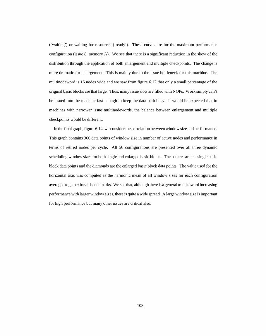
(‘waiting’) or waiting for resources (‘ready’). These curves are for the maximum performance

configuration (issue 8, memory A). We see that there is a significant reduction in the skew of the

distribution through the application of both enlargement and multiple checkpoints. The change is

more dramatic for enlargement. This is mainly due to the issue bottleneck for this machine. The

multinodeword is 16 nodes wide and we saw from figure 6.12 that only a small percentage of the

original basic blocks are that large. Thus, many issue slots are filled with NOPs. Work simply can’t

be issued into the machine fast enough to keep the data path busy. It would be expected that in

machines with narrower issue multinodewords, the balance between enlargement and multiple

checkpoints would be different.

In the final graph, figure 6.14, we consider the correlation between window size and performance.

This graph contains 366 data points of window size in number of active nodes and performance in

terms of retired nodes per cycle. All 56 configurations are presented over all three dynamic

scheduling window sizes for both single and enlarged basic blocks. The squares are the single basic

block data points and the diamonds are the enlarged basic block data points. The value used for the

horizontal axis was computed as the harmonic mean of all window sizes for each configuration

averaged together for all benchmarks. We see that, although there is a general trend toward increasing

performance with larger window sizes, there is quite a wide spread. A large window size is important

for high performance but many other issues are critical also.

108

0

1

2

3

4

5

6

7

8

9

1 2 3 4 5 6 7 80

1

2

3

4

5

6

7

8

9

1 2 3 4 5 6 7 8

ss

ds, w=1

ds, w=4

ds, w=1, enl.

ss, enl.

ds, w=4, enl.

ds, w=256

ds, w=256, enl.

ds, w=4, enl., 100%bp

ds, w=256, enl., 100%bp

Spee

dup

Ove

r Se

quen

tial,

Stat

ical

ly S

ched

uled

Mac

hine

Issue Model

Figure 6.6

Issue Model Summary(Memory Configuration = A)

109

0

1

2

3

4

5

6

7

8

9

A E D B G F C0

1

2

3

4

5

6

7

8

9

A E D B G F C

ss

ds, w=1

ds, w=1, enl.

ss, enl.

ds, w=4, enl.

ds, w=256

ds, w=256, enl.

ds, w=4, enl., 100%bp

ds, w=256, enl., 100%bp

Spee

dup

Ove

r Se

quen

tial,

Stat

ical

ly S

ched

uled

Mac

hine

Memory Configuration

Figure 6.7

Memory Configuration Summary(Issue Model = 8)

ds, w=4, enl.

110

0

1

2

3

4

5

6

7

8

9

1C 2C 2F 3F 3G 4G 4B 5B 5D 6D 6E 7E 7A 8A

Issue Model / Memory Configuration

Figure 6.8

Benchmark Summary(Dynamic Scheduling, Window = 4, Enlargement)

grep

sort

diff

compress

cpp

Spee

dup

Ove

r Se

quen

tial,

Stat

ical

ly S

ched

uled

Mac

hine

111

0

0.1

0.2

0.3

0.4

0.5

1 2 3 4 5 6 7 80

0.1

0.2

0.3

0.4

0.5

1 2 3 4 5 6 7 8

Figure 6.9

Static vs. Dynamic Scheduling(Dynamic Window=1, Enlargement)

memory C

memory F

memory Gmemory B

memory D

memory E

memory A

Issue Model

Add

ition

al N

odes

per

Cyc

le o

f D

ynam

ic S

ched

ulin

g ov

er S

tatic

Sch

edul

ing

112

0

0.5

1

1.5

1 2 3 4 5 6 7 80

0.5

1

1.5

1 2 3 4 5 6 7 8

Figure 6.10

Dynamic Scheduling Window(Enlargement)

Issue Model

Add

ition

al N

odes

per

Cyc

le o

f W

indo

w S

ize

Four

ove

r W

indo

w S

ize

One

memory Amemory Dmemory Ememory Bmemory Fmemory Gmemory C

113

0.65

0.7

0.75

0.8

0.85

0.9

0.95

1

1 2 3 4 5 6 7 80.65

0.7

0.75

0.8

0.85

0.9

0.95

1

1 2 3 4 5 6 7 8

Figure 6.11

Operation Redundancy

Issue Model

Num

ber

of N

odes

Sch

edul

ed /

Num

ber

of N

odes

Ret

ired

ssds, w=1

ds, w=4

ds, w=1, enl.

ss, enl.

ds, w=4, enl.

ds, w=256

ds, w=256, enl.

114

0

0.1

0.2

0.3

0.4

0.5

0.6

0 5 10 15 20 25 30 35 40 45 50 55 60 65 70 75 80 85 90 95+

Figure 6.12

EAU Size Histograms for Single and Enlarged Basic Blocks

Number of Nodes per Execution Atomic Unit

single basic blocks

enlarged basic blocks

115

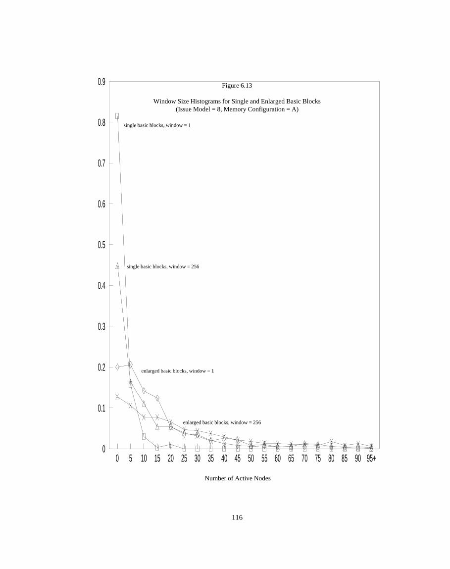
0

0.1

0.2

0.3

0.4

0.5

0.6

0.7

0.8

0.9

0 5 10 15 20 25 30 35 40 45 50 55 60 65 70 75 80 85 90 95+

Figure 6.13

Window Size Histograms for Single and Enlarged Basic Blocks(Issue Model = 8, Memory Configuration = A)

Number of Active Nodes

single basic blocks, window = 1

enlarged basic blocks, window = 1

single basic blocks, window = 256

enlarged basic blocks, window = 256

116

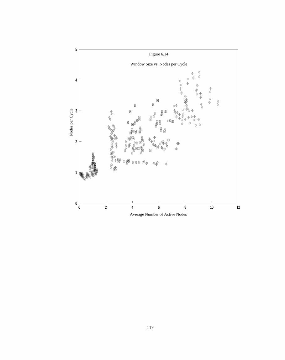
0 2 4 6 8 10 120

1

2

3

4

5Figure 6.14

Window Size vs. Nodes per Cycle

Average Number of Active Nodes

Nod

es p

er C

ycle

0 2 4 6 8 10 120

1

2

3

4

5

117

Chapter 7 Conclusions

Engineering involves the analysis of tradeoffs. In the case of computer engineering this analysis

is particularly complex since solutions typically have few constraints. Modern computer systems

are so complex that the tradeoffs are usually difficult to understand completely. Decisions at one

level may have wide reaching effects on other levels. Thus, an important facet of any serious

computer design project is the careful consideration of how to allocate resources among the different

levels of the machine. This fact has long been appreciated by most computer engineers. The

following quote comes from 1946 in a discussion about which functions to include in an arithmetic

unit by Burks, Goldstine and von Neuman:

“We wish to incorporate into the machine -- in the form of circuits -- only such logical conceptsas are either necessary to have a complete system or highly convenient because of the frequencywith which they occur and the influence they exert in the relevant mathematical situations. ” 1

Another early reference comes from 1962 in the description of project STRETCH in which Werner

Buchholz states a guiding principle as follows:

“The objective of economic efficiency was understood to imply minimizing the cost of answers,not just the cost of hardware. This meant repeated consideration of the costs associated withprogramming, compilation, debugging, and maintenance, as well as the obvious cost ofmachine time for production computation. ... A corollary of this principle was the recognitionthat complex tasks always entail a price in information (and therefore money) and that thisprice is minimized by selecting the proper form of payment -- sometimes extra hardware,sometimes extra instruction executions, and sometimes harder thought in developing program-ming systems.” 2

The 1980’s have brought significant changes in processor design. Microprocessors have made

great strides, eroding the mini and mainframe markets. In many cases, new processors have been

designed with more functionality in software and less in hardware. Some have suggested that these

changes have been the result of the basic principle stated above, that of optimizing hardware/software

tradeoffs, being discovered. Was it forgotten in the 1970’s and re-discovered in the 1980’s?

118

1 [BuGv46]; from [Taub63]; from [BeNe71], p. 982 [Buch62], pp. 7 - 8

Actually, this design principle has always been applied; here a different phenomenon has been at

work.

Ever since the first stored program computer was designed 40 years ago, microarchitecture and

compiler technology have both evolved tremendously. Some of these changes are: different ratios

of processor speed and memory speed, increasing significance of chip boundaries and improved

compiler technology. At each step in this evolution, computer designers have attempted to strike a

balance in the placement of functionality. At various times certain functions have been moved from

hardware to software and vice versa, and this movement is likely to continue. It has been this change

in technology, not a change in design philosophy which has caused tradeoffs to be optimized in

different ways. Thus, what we have witnessed in the 1980’s has been an evolution in the field of

computer engineering, not a revolution.

Continuing this process of evolution, this dissertation has explored the notion of employing

advanced hardware techniques for exploiting fine grained parallelism in general purpose instruction

streams. By providing more background for the analysis of hardware/software tradeoffs, we can

better understand what the limits of single instruction stream processors are and better assess how

to most cost-effectively allocate resources within a computer system. In this chapter we will first

draw on the simulation results from the previous chapter as well as ideas from other chapters and

focus on the limits to performance in single instruction streams. In the second and final section we

will discuss several areas of future research.

7.1 Limits of Single I-Stream Processors

In this dissertation we have identified three closely related hardware concepts and explored their

effectiveness (see Table 7.1). They are dynamic scheduling, dynamic branch prediction and basic

block enlargement. The key ideas behind each of these concepts are node decoupling, speculative

execution and assert nodes respectively. We have shown that through the application of these

techniques, more parallelism can be exploited than is generally recognized to be present in general

purpose instruction streams.

119

The first idea, node decoupling, involves allowing nodes within each multinodeword (i.e. the group

of nodes issued into the machine in each cycle) to be scheduled independently. Decoupling is an

unbinding of the processes of issuing and scheduling. The advantages of decoupling fall into two

main categories. First, it allows memory reads to be re-ordered at run-time. This is advantageous

when the latency for a memory read can vary (e.g. due to a cache miss). By decoupling, other nodes

are not slowed down by the node which has to wait. The ability to disambiguate memory addresses

at run-time is another performance advantage of allowing memory reads to be re-ordered. Hardware

can check memory addresses and determine if preserving instruction stream order is necessary. The

second main category of decoupling advantages has to do with execution efficiency. In short, it

allows speculative execution to be exploited more efficiently. Both non-decoupled and decoupled

machines can take advantage of speculative execution, but, with decoupling, the advantages of larger

basic blocks can be traded off with the advantages of having multiple checkpoints with intermediate

backup capability.

Table 7.1Performance Enhancement Concepts

Concept Key Idea Performance Implications

DynamicScheduling

Node Decoupling Allows Dynamic Re-ordering of Memory Reads cache misses dynamic address disambiguationMore Efficient Use of Speculative Execution higher issue bandwidth intermediate backup for higher efficiency

Dynamic BranchPrediction

Speculative Execution Exploitation of Parallelism Across Basic Blocks no fix-up code dynamic branch conditionsAbility to Exploit Assert Nodes

Basic BlockEnlargement

Assert Nodes Static Optimization of Large Units of Work re-optimization across branches fewer named registers requiredBetter Utilization of Issue BandwidthEfficiency Tradeoff With Node Decoupling

120

Speculative execution is the second main idea discussed in this dissertation. It allows parallelism

to be exploited across branches without the need for fix-up code and without having to statically

determine branch directions. Speculative execution also allows assert nodes to be implemented,

which are the third key idea. Speculative execution is closely tied to decoupling and assert nodes.

The way it is exploited depends on whether decoupling is present and whether assert nodes are

implemented.

Assert nodes allow multiple basic blocks to be packed together and optimized as a single unit.

This is advantageous from the standpoint of eliminating redundant nodes and maximizing issue

bandwidth. In the case of a decoupled machine, a tradeoff exists between the size of the enlarged

basic blocks created with assert nodes and the size of the instruction window. If the former is too

large and the latter too small, performance will suffer from a low execution efficiency. A large number

of nodes will be discarded due to branch faults.

In chapter 6 we presented simulation results showing realistic processors exploiting these three

ideas achieving speedup in excess of 4 on non-scientific benchmarks. Given the complexity of the

hardware required, some might consider this an upper bound on the performance of single instruction

stream processors. Actually, we consider this more of a lower bound. There are many unexplored

avenues which should be able to push the degree of parallelism even higher. First, we have not fully

optimized the use of the techniques analyzed. Better branch prediction could have been used, and

the implementation of basic block enlargement could have been improved. There are also many

issues we did not address directly in this dissertation. In the remainder of this section we will examine

two areas in which artificial limits are typically placed on single instruction stream processors: by

the architecture and by the compiler.

7.1.1 Architectural Considerations

As hardware and software technology evolves, the instruction set architecture best matched to that

technology also changes. This presents a basic dilemma. By decoupling the architecture from a

particular implementation, a company preserves investment in object code and compilers, and can

121

easily market a family of compatible products. However, once an architecture is successful, it dies

very slowly, even after technological changes have made previous tradeoffs no longer appropriate.

Sometimes the mismatch between the architecture and the implementation can be so large as to

significantly hamper performance. In many cases, however, a mismatch between the architecture

and the implementation will not cause a serious performance penalty if a little effort is made and a

few clever ideas are introduced. However, suppose we are given a blank slate. Let us consider some

of the ideal characteristics for an instruction set architecture given an implementation incorporating

the mechanisms discussed in the previous chapters.

There are many constraints imposed on the implementation by the instruction stream format, as

opposed to its semantic content. Ideally, there should be no implicit sequentiality, such as sequentially

defined, microcode-based decode syntax. Instead, the instruction stream should be formatted into a

data flow graph. This does not mean that there should be no encoding, only that the decoding should

be able to proceed in parallel as much as possible. Another ideal feature is that instruction stream

should be formatted into EAUs, whatever size they are, with header information at the beginning of

the EAU. Thus, for basic block EAUs, the processor can fetch the entry point to the basic block and

immediately determine how large it is and how it is resolved (e.g. branch through a memory node,

two way branch to explicit addresses, and so on).

Related to these issues but having to do with the semantics of the instruction stream itself are

several other desirable features. The use of global condition codes is a concept whose time has gone.

By eliminating condition codes and having nodes refer explicitly to the results of other nodes,

enforcing flow dependencies while eliminating all others gets easier. Another helpful concept is the

separation of control from data. In particular, return addresses can be maintained separately to speed

up the fetching and decoding of the instruction stream when a return is encountered. This technique

can be applied to calls and returns as well as interrupt and exception entries and exits. Minimizing

dynamic branches also helps in this regard. Architectural features such as jump tables and case

statements require dynamic branches in addition to language features such as being able to pass

122

functions as parameters. Thus, some sort of tradeoff is necessary. How important are the architec-

tural and language features and can they be restricted without causing problems for compiler writers?

A concept often overlooked is the complication in dealing with memory mapped I/O. In a machine

which supports dynamic branch prediction and out of order execution, the order of memory accesses

is not guaranteed within the instruction window (which may bridge several unconfirmed branches).

This is not acceptable for I/O devices because reads typically have side-effects. By separating

memory from I/O, the processor can more cleanly enforce read-after-read dependencies without

having to resort to run-time tests to distinguish the addresses.

Interrupt and exception precision is another important issue. If the AAU size is the same as the

EAU size, then the processor does not have to have additional hardware to step through AAUs to

recreate a boundary which was dissolved in the EAU creation process. This will involve some higher

level software issues. If we force precision at a level as large as an enlarged basic block, it may be

difficult in some circumstances to determine the exact node which caused the problem. This can be

alleviated somewhat by adding node and operand information to the exception frame before the

exception handler is called.

Another beneficial side-effect of having large AAUs is that fewer architectural registers are

needed. Only results which are written in one basic block and are needed in another basic block need

to be put into named registers. Our simulations have shown that the number of register writes within

an enlarged basic block was typically less than two. In other words, the number of general purpose

registers could have been reduced to a very small number without hampering performance. The

importance of large numbers of internal temporary registers should not be confused with the need

for architectural registers.

Note that large EAUs does not necessitate longer interrupt latency. If low interrupt latency is

critical and if the interrupt rate is low enough, the EAU which is being executed can be thrown away.

That is, an interrupt can force an immediate fault and when the interrupt routine is over the faulted

basic block can be re-issued.

123

There are also many architectural issues which relate directly to the language and application.

First, the choice of nodes itself is critical. The primitives used should be well matched to the higher

levels. For example, in our simulator, we implemented an INDX4 node which adds its first operand

to its second operand shifted two bits to the left. In terms of ALU complexity, this is little more than

an add, but it will save a node and a stage in the dependency chain when indexing arrays of 4 byte

elements. If this node is present as a primitive, then obviously the compiler needs to know about it.

(In our study, because VAX code was used as the source, most of the array indexing was done using

VAX indexed addressing modes, so the translating loader could detect these cases. If we had been

simulating from code for a more primitive architecture, it would have been harder to detect and

optimize for this case.)

Finally, consider how language/architecture optimizations go the other way, that is how architec-

ture affects language. The definition of programming languages has always been tied somewhat to

processor architectures, in some cases more closely than others. C is a good example of a language

that was defined with efficient execution in mind. Run-time array bounds checking was left out of

the language specification, presumably because on a conventional machine it can be a significant

performance penalty. However, with dynamic branch prediction array bounds checking can become

very inexpensive. The nodes which verify that indices are in bounds can be packed into the basic

block in places that might otherwise contain NOPs. If the indices are in bounds, the nodes would

execute silently and signal otherwise. There are other ways in which assert nodes can be exploited

for their ability to optimize for low frequency branches. Thus, future languages which can benefit

from this and other architectural features are likely to change in the things that are defined.

7.1.2 Compiler Techniques

Now that we have looked at architectural features which limit performance, we will consider

compiler technology. Compilers have great potential in allowing more parallelism to be exploited.

Contrary to what some have suggested, dynamic scheduling does not obviate a complex compiler,

124

it just changes some of the mechanisms that are needed. Wider multinodewords put more pressure

on both the hardware and the compiler to find more parallelism to exploit.

The importance of optimizing for a particular EAU size is often overlooked. The code for large

EAUs, for example enlarged basic blocks, needs to be optimized in view of EAU size. The whole

process of allocating registers and eliminating common sub-expressions and redundant memory

operations is tied to the EAU size for which it is done. There are hardware techniques for doing this,

but typically this job would fall on the compiler. The process of enlarging basic blocks itself is

typically a compiler intensive process.

The ordering of nodes within the basic block is also important. Dynamically scheduled processors

typically schedule oldest node first. This means that the priority of nodes will be determined by the

placement within the instruction stream. By putting important nodes, for example branch confirma-

tion nodes, early in the basic block the scheduling priority can be set. There are other ways also in

which with knowledge of how the processor will schedule, the compiler can put more parallelism

within the instruction window. This lowers hardware cost by allowing higher performance for a

given window size.

Compile-time hints on branch direction is also a must. The first time a branch is encountered,

before run-time information can be used, the compiler is best equipped to make a determination about

which direction should be predicted. This can be a significant performance bonus since branch

density is typically highly skewed. A significant percentage of branch are executed a very small

number of times within the program.

Another area of great potential is the application of advanced basic block enlargement techniques.

One technique which could be employed to advantage is the implementation of multi-way branches.

We have shown how multiple nodes within an enlarged basic block can point to other nodes as branch

fault nodes. It is also the case that more than one of the arcs leaving a basic block can be trap arcs

instead of fault arcs. By combining two sides of a branch which both have no side effects, it is

possible to create a basic block with multiple trap nodes. This is not as uncommon as it might seem.

125

This would be the case if a value is computed and a branch is made based on that value but it is never

used for any other purpose. Thus, it is possible to create multi-way branches in which multiple tests

are done within a basic block and one of many trap arcs signals which basic block to continue with.

7.2 Areas of Future Research

We conclude this dissertation with a discussion of several areas of future research. In the preceding

section we have touched on many areas where more study is required. In this section we will focus

on two particular areas which are more long term in nature: multiple instruction stream processors

and adaptive basic block enlargement techniques.

7.2.1 Multiple Instruction Stream Processors

In this dissertation we have focused on enhancing the performance of single instruction stream

processors. In the introduction some of the tradeoffs between inter-instruction stream and intra-in-

struction stream parallelism were discussed. We implicitly assumed that a given processor would

only be executing a single instruction stream at any given time. Alternatively, a single processor

could simultaneously execute multiple instruction streams. In such a processor, all of the instruction

streams share the same ALUs, paths to memory and register files. (However, there may be

restrictions on the sharing of registers between instruction streams.) The advantage of such a

processor is that it can exploit inter-instruction stream parallelism to keep ALUs and paths to memory

fully utilized.

Figure 7.1 shows a graph of parallelism exploited on single processors. The horizontal axis is the

degree of intra-instruction stream parallelism exploited (in terms of the number of simultaneously

executing nodes per instruction stream) and the vertical axis is the degree of inter-instruction stream

exploited (in terms of the number of simultaneously executing instruction streams).

Conventional processors do not exploit much of either type of parallelism. Only one instruction

stream is executing at a time and usually a small number of nodes are simultaneously executing.

Techniques such as we have described in this dissertation have focused on moving horizontally on

126

the graph. There is still only one instruction stream being executed at a time, but there may be a

large number of simultaneously executing nodes.

The HEP-1 was a departure in that it moved vertically. It was able to exploit parallelism across

instruction streams but there was no intra-instruction stream parallelism possible. Within an

instruction stream, each node was fully executed before the next node started execution. The Horizon

couples the multiple instruction stream concept of the HEP-1 with the ability to exploit parallelism

within an instruction stream as well. The compiler specifies the dependencies between instruction

words, but the Horizon is not a fully decoupled microarchitecture. The nodes within an instruction

word all execute together. It is similar to a statically scheduled wide word machine except that instead

Intra-Instruction Stream ParallelismAverage Number of Simultaneously Executing Nodes per Instruction Stream

1

Inte

r-In

stru

ctio

n St

ream

Par

alle

lism

Ave

rage

Num

ber

of S

imul

tane

ousl

y E

xecu

ting

Inst

ruct

ion

Stre

ams

1Conventional

ProcessorsDecoupledProcessors

HEP-1Horizon

?

Figure 7.1

127

of stalling the pipeline or inserting NOPs when parallelism cannot be found, other instruction streams

are executed.

From the other perspective, imagine how one would modify a processor incorporating the features

described in this dissertation such that it could execute multiple instruction streams. The most general

solution would be to attach process identification tags to nodes within the machine. Then merging,

scheduling and distribution would simply operate on a pool of nodes as before but they would belong

to different instruction streams. This would allow the processor to freely trade off inter- and

intra-instruction stream parallelism. One problem to overcome is that when a trap or fault occurs in

a particular instruction stream, it must be possible to backup to a previous consistent state in that

instruction stream only without affecting other instruction streams.

In a processor of this sort, an important issue becomes the sharing of registers between instruction

streams. At one extreme (exhibited by the HEP-1) is a single register file which all instruction streams

can access uniformly. This imposes significant constraints on the register file in terms of access time

and/or the number of ports needed. At the other extreme would be a case where no sharing could

take place at all. This would allow the registers to be banked in such a way that they become less

expensive to implement. However, scheduling constraints may be imposed. The tradeoff between

sharing registers and constraining scheduling must be weighed carefully in light of how the

instruction streams are created and managed in addition to the target job mix.

7.2.2 Adaptive Basic Block Enlargement

The basic block enlargement techniques discussed in chapters 4 and 6 only scratch the surface of

what is possible. With more sophisticated software and hardware techniques, even more parallelism

can be exploited. Ideally, a processor could adaptively enlarge basic blocks in order to take advantage

of parallelism wherever it may be. This concept could be realized in many different ways and to

different extents. A simple start is run-time fault prediction logic which operates analogously to

dynamic branch prediction. The branch target buffer would maintain for a given entry point

information on which other basic block, if any, it has most recently faulted to. Then, code that

128

branches to that entry point can directly branch to a different basic block. (One side-effect of this

scheme is that every basic block must contain assert nodes verifying the entry conditions rather than

assuming entry conditions are correct because a fault must have caused the entry.)

More sophisticated adaptive enlargement techniques could employ hardware and/or software to

re-enlarge basic blocks based on run-time information. The techniques we discussed in chapter 4

and simulated in chapter 6 were based on branch arc densities taken from a sample run of the program.

A processor could maintain this information dynamically and flag basic blocks in which execution

is highly skewed toward one particular next basic block. Extending this concept would be the ability

to enlarge basic block across a dynamic branch. Suppose an address is computed or read from

memory and then used as the next PC, but it is always or almost always the same. A special assert

node could be inserted to check the value of the run-time address and this next basic block could be

combined with the first one.

Adaptive basic block enlargement techniques such as these allows a computer to ‘‘learn’’ as it

gains experience with a particular program how to best optimize execution for that program. This

could involve an actual re-compilation of the program, such that the external code is modified or it

could be confined to the internal state of the processor. In either case, the techniques could allow

future processors to exploit parallelism with much fewer restrictions and in much more dynamic

environments than is currently possible.

129

References

[AcKT86] Acosta, R. D., Kjelstrup, J., and Torng, H. C., ‘‘An Instruction Issuing Approach to

Enhancing Performance in Multiple Functional Unit Processors,’’ IEEE Transactions on

Computers, vol C-35:9, September, 1986, pp. 815-828.

[AgKe82] Agnew, P. W., and Kellerman, A. S., ‘‘Microprocessor Implementation of Mainframe

Processors by Means of Architecture Partitioning,’’ IBM Journal of Research and Develop-

ment, vol. 26:4, July, 1982, pp. 401-412.

[AlBH81] Albert, B., Bode, A., and Händler, W., ‘‘A Case Study in Vertical Migration: The

Implementation of a Dedicated Associative Instruction Set,’’ Microprocessing and Micro-

programming, vol. 8, 1981, pp. 257-262.

[AnST67] Anderson, D. W., Sparacio, F. J., and Tomasulo, R. M., ‘‘The IBM System/360 Model

91: Machine Philosophy and Instruction - Handling,’’ IBM Journal of Research and

Development, vol. 11:1, 1967, pp. 8-24.

[BaIO82] Baba, T., Ishikawa, K., and Okuda, K., ‘‘A Two-Level Microprogrammed Multiprocessor

Computer with Nonnumeric Functions,’’ IEEE Transactions on Computers, vol. C-31:12,

December, 1982, pp. 1142-1156.

[BaSK67] Bashkow, T. R., Sasson, A., and Kronfeld, A., ‘‘System Design of a FORTRAN

Machine,’’ IEEE Transactions on Electronic Computers, Vol. EC-16, No. 4, August, 1967,

pp. 485-499.

[BeNe62] Bell, C. G., and Newell, A., editors, Computer Structures: Readings and Examples,

McGraw-Hill, 1971.

[Bern84] Berndt, H., ‘‘Software Support in Hardware,’’ Microprocessing and Microprogramming,

vol. 13, 1984, pp. 1-9.

[Bern81] Bernhard, R., ‘‘More Hardware Means Less Software,’’ IEEE Spectrum, vol. 18:12,

December, 1981, pp. 30-37.

130

[BiWo86] Birnbaum, J. S., and Worley, W. S. Jr., ‘‘Beyond RISC: High-Precision Architecture,’’

Proceedings of Spring COMPCON 86, March 3-6, 1986, pp. 40-47.

[BoDa84] Bose, P., and Davidson, E. S., ‘‘Design of Instruction Set Architectures for Support of

High-Level Languages,’’ Proceedings of The 11th International Symposium on Computer

Architecture, 1984, pp. 198-206.

[BrAb79] Bridges, C. W., and Abd-alla, A. M., ‘‘Direct Execution of C-String Compiler Texts,’’

Proceedings of the 12th Annual Workshop on Microprogramming, 1979, pp. 84-92.

[Buch62] Buchholz, W., editor, Planning A Computer System, McGraw-Hill, 1962.

[BuFS78] Bürkle, H. J., Frick, A., and Schlier, Ch., ‘‘High Level Language Oriented hardware and

the Post-von Neumann Era,’’ Proceedings of The 5th Annual Symposium on Computer

Architecture, April 3-5, 1978, pp. 60-65.

[BuGv46] Burks, A. W., Goldstine, H. H., and von Neumann, J., "Preliminary discussion of the

logical design of an electronic computing instrument," report to the U.S. Army Ordnance

Department, 1946 (reproduced in [Taub63], [BeNe71]).

[ChSm71] Chesley, G. D., and Smith, W. R., ‘‘The Hardware-Implemented High-Level Machine

Language for SYMBOL,’’ AFIPS Conference Proceedings, 1971 Spring Joint Computer

Conference, pp. 563-573.

[CHKW86] Chow, F., Himelstein, M., Killian, E., and Weber, L., ‘‘Engineering a RISC Compiler

System,’’ Proceedings of Spring COMPCON 86, March 3-6, 1986, pp. 132-137.

[Chu79] Chu, Y., ‘‘Architecture of a Hardware Data Interpreter,’’ IEEE Transactions on Computers,

Vol. C-28, No. 2, February, 1979, pp. 101-109.

[ChAb81] Chu, Y., and Abrams, M., ‘‘Programming Languages and Direct-Execution Computer

Architecture,’’ Computer, Vol. 14, No. 7, July, 1981, pp. 22-32.

[Chur70] Church, C. C., ‘‘Computer Instruction Repertoire - Time for a Change,’’ AFIPS Conference

Proceedings, 1970 Spring Joint Computer Conference, 1970, pp. 343-349.

131

[ClLe82] Clark, D. W., and Levy, H. M., ‘‘Measurement and Analysis of Instruction Use in the

VAX-11/780,’’ Proceedings, 9th Annual Symposium on Computer Architecture, Austin,

Texas, April, 1982, pp. 9-17.

[COPa83] Colon Osorio, F. C., and Patt, Y. N., ‘‘Tradeoffs in the Design of a System for High Level

Language Interpretation,’’ Proceedings of the International Conference on Computer De-

sign, October, 1983.

[CoHJ83] Colwell, R. P., Hitchcock, C. Y., and Jensen, E. D., ‘‘Peering Through the RISC / CISC

Fog: An Outline of Research,’’ Computer Architecture News, vol. 11:1, March 1983.

[CHJS85] Colwell, R. P., Hitchcock, C. Y., Jensen, E. D., Sprunt, H. M. B., and Kollar, C. P.,

‘‘Computers, Complexity, and Controversy,’’ Computer, vol. 18:9, September, 1985, pp.

8-19.

[CoFl70] Cook, R. W., and Flynn, M. J., ‘‘System Design of a Dynamic Microprocessor,’’ IEEE

Transactions on Computers, Vol. C-19, No. 3, March, 1970, pp. 213-222.

[Ditz80] Ditzel, D. R., ‘‘Program Measurements on a High-Level Language Computer,’’ Computer,

vol. 13:8, August, 1980, pp. 62-71.

[Ditz81] Ditzel, D. R., ‘‘Reflections on the High-Level Language Symbol Computer System,’’

Computer, Vol. 14, No. 7, July, 1981, pp. 55-66.

[Fish81] Fisher, J. A., ‘‘Trace Scheduling: A Technique for Global Microcode Compaction,’’ IEEE

Transactions on Computers, vol. C-30, no. 7, July 1981.

[Flyn74] Flynn, M. J., ‘‘Trends and Problems in Computer Organizations,’’ Proceedings of the

Information Processing Congress, 1974, pp. 3-10.

[Flyn80] Flynn, M. J., ‘‘Directions and Issues in Architecture and Language,’’ Computer, Vol. 13,

No. 10, October, 1980, pp. 5-22.

[Flyn83] Flynn, M. J., ‘‘Towards Better Instruction Sets,’’ Proceedings of the 16th Annual Workshop

on Microprogramming, October 11-14, 1983, pp. 3-8.

132

[FlHo83] Flynn, M. J., and Hoevel, L. W., ‘‘Execution Architecture: The DELtran Experiment,’’

IEEE Transactions on Computers, vol. C-32:2, February, 1983, pp. 156-175.

[FlHo84] Flynn, M. J., and Hoevel, L. W., ‘‘Measures of Ideal Execution Architectures,’’ IBM

Journal of Research and Development, vol. 28:4, July, 1984, pp. 356-369.

[FlJW85] Flynn, M. J., Johnson, J. D., and Wakefield, S. P., ‘‘On Instruction Sets and Their

Formats,’’ IEEE Transactions on Computers, vol. C-34:3, March, 1985, pp. 242-254.

[FlNM75] Flynn, M. J., Neuhauser, C., and McClure, R. M., ‘‘EMMY - An Emulation System for

User Microprogramming,’’ AFIPS Conference Proceedings, The 1975 National Computer

Conference, Vol. 44, May 19-22, 1975, pp. 85-89.

[FoRi72] Foster, C. C., and Riseman, E. M., ‘‘Percolation of Code to Enhance Parallel Dispatching

and Execution,’’ IEEE Transactions on Computers, vol C-21:12, December, 1972, pp.

1411-1415.

[GrKL83] Grossmann, B., Kwee, E., and Lehmann, A., ‘‘Practical Experiences with Vertical

Migration,’’ Microprocessing and Microprogramming, vol. 12, 1983, pp. 185-192.

[HLMM82] Hansen, P. M., Linton, M. A., Mayo, R. N., Murphy, M., and Patterson, D. A., ‘‘A

Performance Evaluation of the Intel iAPX 432,’’ Computer Architecture News, vol. 10:4,

June, 1982.

[HaLL73] Hassitt, A., Lageschulte, J. W., and Lyon, L. E., ‘‘Implementation of a High Level

Language Machine,’’ Communications of the ACM, Vol. 16, No. 4, April, 1973, pp. 199-212.

[HaLy76] Hassitt, A., and Lyon, L. E., ‘‘An APL Emulator on System/370,’’ IBM System Journal,

No. 4, 1976, pp. 358-378.

[Heat84] Heath, J. L., ‘‘Re-Evaluation of the RISC I,’’ Computer Architecture News, vol. 12:1,

March, 1984, pp. 3-10.

[HJGB82] Hennessy, J., Jouppi, N., Gill, J., Baskett, F., Strong, A., Gross, T., Rowen, C., and

Leonard, J., ‘‘The MIPS Machine,’’ Proceedings of Spring COMPCON 82, March 1982,

pp. 2-7.

133

[HJPR82] Hennessy, J., Jouppi, N., Przybylski, S., Rowen, C., Gross, T., Baskett, F., and Gill, J.,

‘‘MIPS: A Microprocessor Architecture,’’ Proceedings of the 15th Annual Workshop on

Microprogramming, October 5-7, 1982, pp. 17-22.

[HiSp85] Hitchcock, C. Y., and Sprunt, H. M. B., ‘‘Analyzing Multiple Register Sets,’’ Proceedings

of The 12th Annual International Symposium on Computer Architecture, June 17-19, 1985,

pp. 55-63.

[Hoev74] Hoevel, L. W., ‘‘’Ideal’ Directly Executed Languages: An Analytical Argument for

Emulation,’’ IEEE Transactions on Computers, Vol. C-23, No. 8, August, 1974, pp.

759-767.

[Hojk81] Hojka, N., ‘‘Increasing Performance by Microcoding,’’ Microprocessing and Micropro-

gramming, vol. 8, 1981, pp. 229-236.

[Holt85] Holtkamp, B., ‘‘UNIX Requirements for Arhcitectural Support,’’ Microprocessing and

Microprogramming, vol. 15, 1985, pp. 129-140.

[Hopk83a] Hopkins, M. E., ‘‘A Perpective on Microcode,’’ Proceedings of Spring COMPCON 83,

February 28 - March 3, 1983, pp. 108-110.

[Hopk83b] Hopkins, W. C., ‘‘HLLDA Defies RISC: Thoughts on RISC’s, CISC’s and HLLDA’s,’’

Proceedings of the 16th Annual Workshop on Microprogramming, October 11-14, 1983, pp.

70-74.

[HuLa85] Huguet, M., and Lang, T., ‘‘A Reduced Register File for RISC Architectures,’’ Computer

Architecture News, vol. 13:4, September, 1985, pp. 22-31.

[Hwu87] Hwu, W. W., ‘‘HPSm: Exploiting Concurrency to Achieve High Performance in a

Single-chip Microarchitecture,’’ Ph.D. Dissertation, University of California, Berkeley,

December, 1987.

[HwPa87] Hwu, W. W., and Patt, Y. N., ‘‘Checkpoint Repair for Out-of-order Execution Machines,’’

Proceedings, 14th Annual International Symposium on Computer Architecture, June 2-5,

1987, Pittsburgh, PA.

134

[HwPa86] Hwu, W. W., and Patt, Y. N., ‘‘HPSm, A High Performance Restricted Data Flow

Architecuture Having Minimal Functionality,’’ Proceedings, 13th Annual International

Symposium on Computer Architecture, Tokyo, June 1986.

[JoWa89] Jouppi, N. P., and Wall, D. W., ‘‘Available Instruction-Level Parallelism for Superscalar

and Superpipelined Machines,’’ Proceedings, Third International Conference on Architec-

tural Support for Programming Languages and Operating Systems, Boston, MA, April 3-6,

1989, pp. 272-282.

[Katz71] Katzan H. Jr., Computer Organization and the System/370, Van Nostrand Reinhold

Company, 1971.

[KBBD82] Kavi, K., Belkhouche, B., Bullard, E., Delcambre, L., and Nemecek, S., ‘‘HLL Archi-

tectures: Pitfalls and Predilections,’’ Proceedings of the 9th Annual Symposium on Computer

Architecture, April 26-29, 1982, pp. 18-23.

[Kell75] Keller, R. M., ‘‘Look Ahead Processors,’’ Computing Surveys, vol. 7:4, Dec. 1975.

[KoRi84] Korthauer, E., and Richter, L., ‘‘Are RISCs Subsets of CICSs? A Discussion of Reduced

versus Complex Instruction Sets,’’ Microprocessing and Microprogramming, vol. 14, 1984,

pp. 1-8.

[KuMC72] Kuck, D. J., Muraoka, Y., and Chen, S-C., ‘‘On the Number of Operations Simulta-

neously Executable in Fortran-Like Programs and Their Resulting Speedup,’’ IEEE Trans-

actions on Computers, vol. C-21:12, December, 1972, pp. 1293-1310.

[KBCL74] Kuck, D. J., Budnik, P. P., Chen, S-C., Lawrie, D. H., Towle, R. A., Strebendt, R. E.,

Davis, E. W., Han, J., Kraska, P. W., and Muraoka, Y., ‘‘Measurments of Parallelism in

Ordinary FORTRAN Programs,’’ IEEE Computer, January, 1974, pp. 37-45.

[Laws68] Lawson , H. W., ‘‘Programming-Language-Oriented Instruction Streams,’’ IEEE Trans-

actions on Computers, vol. C-17:5, May, 1968, pp. 476-485.

[Lund77] Lunde, A., ‘‘Empirical Evaluation of Some Features of Instruction Set Processors Archi-

tectures,’’ Communications of the ACM, vol. 20:3, March 1977, pp 143-153.

135

[LuRi81] Luque, E., and Ripoll, A., ‘‘Microprogramming: A Tool for Vertical Migration,’’

Microprocessing and Microprogramming, Vol. 8, 1981, pp. 219-228.

[Mack81] Mackrodt, W., ‘‘Considerations on Language Interpretation for Microprocessor Sys-

tems,’’ Microprocessing and Microprogramming, vol. 7, 1981, pp. 110-118.

[Mand72] Mandell, R. L., ‘‘Hardware/Software Trade-Offs - Reasons and Directions,’’ AFIPS

Conference Proceedings, 1972 Fall Joint Computer Conference, vol. 41, 1972, pp. 453-459.

[Mark81] Markowitz, R. J., ‘‘Software Impact on Microcomputer Architecture, A Case Study,’’

Proceedings of the 8th Annual Symposium on Computer Architecture, 1981, pp. 40-48.

[MePa87] Melvin, S. W., and Patt, Y. N., ‘‘A Clarification of the Dynamic/Static Interface,’’

Proceedings, 20th Hawaii International Conference on System Sciences, January 6-9, 1987,

Kailua-Kona, HI.

[MePa89] Melvin, S. W., and Patt, Y. N., ‘‘Performance Benefits of Large Execution Atomic Units

in Dynamically Scheduled Machines,’’ Proceedings, 1989 Supercomputer Conference,

Crete, Greece.

[MeSP88] Melvin, S. W., Shebanow, M. C., and Patt, Y. N., ‘‘Hardware Support for Large Atomic

Units in Dynamically Scheduled Machines,’’ Proceedings, 21st Annual Workshop on

Microprogramming and Microarchitecture, San Diego, CA, November 1988.

[MWSH87] Melvin, S. W., Wilson, J., Shebanow, M., Hwu, W. and Patt, Y., ‘‘On Tuning the

Microarchitecture of an HPS Implementation of the VAX,’’ Proceedings, 20th Annual

Workshop on Microprogramming, December 1-4, 1987, Colorado Springs, CO.

[MCFH86] Moussouris, J., Crudele, L., Freitas, D., Hansen, C., Hudson, E., March, R., Przybylski,

S., Riordan, T., Rowen, C. and Van’t Hof, D., ‘‘A CMOS RISC Processor With Integrated

System Functions,’’ Proceedings of COMPCON 86, March 3-6, 1986, pp. 126-131.

[Myer80] Myers, G. J., Advances in Computer Architecture, 2nd edition, John Wiley and Sons, 1982.

136

[NiFi84] Nicolau, A., and Fisher, J. A., ‘‘Measuring the Parallelism Available for Very Long

Instruction Word Architectures,’’ IEEE Transactions on Computers, vol. C-33:11, Novem-

ber, 1984, pp. 968-976.

[NoAb83] Norton, R. L., and Abraham, J. A., ‘‘Adaptive Interpretation as a Means of Exploiting

Complex Instruction Sets,’’ Proceedings of The 10th Annual International Symposium on

Computer Architecture, 1983, pp. 277-282.

[Obre82] Obrebska, M., ‘‘Efficiency and Performance Comparison of Different Degisn Methodol-

ogies for Control Parts of Micrprocessors,’’ Microprocessing and Microprogramming, vol.

10, 1982, pp. 163-178.

[OrHi78] Organick, E. I., and Hinds, J. A., Interpreting Machines: Architecture and Programming

of the B1700/B1800 Series, Elsevier North-Holland, Inc., 1978.

[PaAh85] Patt, Y. N., and Ahlstrom, J. K., ‘‘Microcode and the Protection of Intellectual Effort,’’

Proceedings of the 18th Annual Workshop on Microprogramming, Pacific Grove, CA,

December 3-6, 1985, pp. 167-170.

[PaHS85] Patt, Y. N., Hwu, W. W., and Shebanow, M. C., ‘‘HPS, A New Microarchitecture:

Rationale and Introduction,’’ Proceedings, 18th Annual Workshop on Microprogramming,

December 3-6, 1985, Asilomar, CA.

[PMHS86] Patt, Y., Melvin, S., Hwu, W., Shebanow, M., Chien, C., and Wei, J., ‘‘Run-Time

Generation of HPS Microinstructions from a VAX Instruction Stream,’’ Proceedings, 19th

Annual Workshop on Microprogramming, October 15-17, 1986, New York, NY.

[PMHS86] Patt, Y. N., Melvin, S. W., Hwu, W., Shebanow, M. C. Chien, C., and Wei, J., ‘‘Run-time

Generation of HPS Microinstructions From a VAX Instruction Stream,’’ Proceedings, 19th

Annual Workshop on Microprogramming, October 15-17, 1986, New York, NY.

[PMHS85] Patt, Y. N., Melvin, S. W., Hwu, W. W., and Shebanow, M. C., ‘‘Critical Issues Regarding

HPS, A High Performance Microarchitecture,’’ Proceedings, 18th Annual Workshop on

Microprogramming, December 3-6, 1985, Asilomar, CA.

137

[PSHM86] Patt, Y. N., Shebanow, M. C., Hwu, W., and Melvin, S. W., ‘‘A C Compiler for HPS I,

A Highly Parallel Execution Engine,’’ Proceedings, 19th Hawaii International Conference

on System Sciences, Honolulu, HI, January 1986.

[PGHL83] Patterson, D. A., Garrison, P., Hill, M., Lioupis, D., Nyberg, C., Sippel, T., and Van Dyke,

K., ‘‘Architecture of a VLSI Instruction Cache for a RISC,’’ Proceedings of The 10th Annual

International Symposium on Computer Architecture, 1983, pp. 108-116.

[PaHe85] Patterson, D., and Hennessy, J., ‘‘Response to ‘Computers, Complexity, and Controversy’,

’’ Computer, vol. 18:11, November, 1985, pp. 142-143.

[PaPi82] Patterson, D. A., and Piepho, R. S., ‘‘Assesing RISCs in High-Level Language Support,’’

IEEE Micro, vol. 2:4, November, 1982, pp. 9-19.

[PaSe80] Patterson, D. A., and Sequin, C. H., ‘‘Design Considerations for Single-Chip Computers

of the Future,’’ IEEE Transactions on Computers, vol. C-29:2, February, 1980, pp. 108-116.

[Piep81] Piepho, R. S., ‘‘Comparative Evaluation of the RISC I Architecture via the Computer

Family Architecture Bechmarks,’’ University of California at Berkeley, EECS Master’s

Report, August 27, 1981.

[Pihl80] Pihlgren, G., ‘‘Increasing Performance in a Cobol System by Adding Firmware,’’ EU-

ROMICRO Journal, Vol. 6, 1980, pp. 403-405.

[Radi83] Radin, G., ‘‘The 801 Minicomputer,’’ IBM Journal of Research and Development, Vol.

27, No. 3, May 1983, pp. 237-246.

[RaTs70] Rammamoorthy, C. V., and Tsuchiya, M., ‘‘A Study of User-Microprogrammable Com-

puters,’’ AFIPS Conference Proceedings, 1970 Spring Joint Computer Conference, Vol. 40,

1970, pp. 165-181.

[RaAg78] Rauscher, T. G., and Agrawala, A. K., ‘‘Dynamic Problem-Oriented Redefinition of

Computer Architecture via Microprogramming,’’ IEEE Transactions on Computers, Vol.

C-27, No. 11, November, 1978, pp. 1006-1014.

138

[ReFF72] Reigel, E. W., Faber, U., and Fisher, D. A., ‘‘The Interpreter - A Microprogrammable

Building Block System,’’ AFIPS Conference Proceedings, 1972 Spring Joint Computer

Conference, May 16-18, 1972, pp. 705-723.

[ReMc83] Requa, J. E., and McGraw, J. R., ‘‘The Piecewise Data Flow Architecture: Architectural

Concepts,’’ IEEE Transactions on Computers, vol. C-35:5, May, 1983, pp. 425-438.

[Rice81] Rice, R., ‘‘The Chief Architect’s Reflections on Symbol IIR,’’ Computer, Vol. 14, No. 7,

July, 1981, pp. 49-54.

[RiSm71] Rice, R., and Smith, W. R., ‘‘SYMBOL - A Major Departure From Classic Software

Dominated von Neumann Computing Systems,’’ AFIPS Conference Proceedings, 1971

Spring Joint Computer Conference, pp. 575-587.

[RiFo72] Riseman, E. M., and Foster, C. C., ‘‘The Inhibition of Potential Parallelism by Conditional

Jumps,’’ IEEE Transactions on Computers, vol C-21:12, December, 1972, pp. 1405-1411.

[ShGi83] Sheraga, R. J., and Gieser, J. L., ‘‘Experiments in Automatic Microcode Generation,’’

IEEE Transactions on Computers, vol. C-32:6, June, 1983, pp. 557-569.

[SmJH89] Smith, M. D., Johnson, M., Horowitz, M. A., ‘‘Limits on Multiple Instruction Issue,’’

Proceedings, Third International Conference on Architectural Support for Programming

Languages and Operating Systems, Boston, MA, April 3-6, 1989, pp. 290-302.

[Smit78] Smith, B. J., ‘‘A Pipelined Shared Resource MIMD Computer,’’ Proceedings, 1978

International Conference on Parallel Processing, 1978.

[Smit89] Smith, J. E., ‘‘Dynamic Instruction Scheduling and the Astronautics ZS-1,’’ Computer,

July, 1989, pp. 21-35.

[SmLH90] Smith, M. D., Lam, M. S., and Horowitz, M. A., ‘‘Boosting Beyond Static Scheduling

in a Superscalar Processor,’’ Proceedings, 17th Annual International Symposium on Com-

puter Architecture, Seattle, WA, May 28-31, 1990, pp. 344-353.

[SRCL71] Smith, W. R., Rice, R., Chesley, G. D., Laliotis, T. A., Lundstrom, S. F., Calhoun, M. A.,

Gerould, L. D., and Cook, T. G., ‘‘SYMBOL - A Large Experimental System Exploring

139

Major Hardware Replacement of Software,’’ AFIPS Conference Proceedings, 1971 Spring

Joint Computer Conference, pp. 601-616.

[Sohi90] Sohi, G. S., ‘‘Instruction Issue Logic for High-Performance, Interruptible, Multiple Func-

tional Unit, Pipelined Computers,’’ IEEE Transactions on Computers, vol. 39:3, March

1990, pp. 349-359.

[Stan81] Stankovic, J. A., ‘‘The Types and Interactions of Vertical Migrations of Functions in a

Multilevel Interpretive System,’’ IEEE Transactions on Computers, vol. C-30:7, July, 1981,

pp. 505-513.

[Stva81] Stockenberg, J., and van Dam, A., ‘‘Vertical Migration for Performance Enhancement in

Layered Hardware/Firmware/Software Systems,’’ Computer, vol. 11:5, May, 1978, pp.

35-50.

[TaSe83] Tamir, Y., and Sequin, C. H., ‘‘Strategies for Managing the Register File in RISC,’’ IEEE

Transactions on Computers, vol. C-32:11, November, 1983, pp. 977-989.

[Tane78] Tanenbaum, A. S., ‘‘Implications of Structured Programming for Machine Architecture,’’

Communications of the ACM, vol. 21:3, March, 1978, pp. 237-246.

[Tane84] Tanenbaum, A. S., Structured Computer Organization, 2nd edition Prentice-Hall, Inc.,

Englewood Cliffs, N. J., 1984.

[Taub63] Taub, A. H., editor, ‘‘Collected Works of John von Neumann,’’ vol. 5, pp. 34-79, The

Macmillan Company, New York, 1963 (excerpt [BuGv46] reproduced in [BeNe71]).

[Thom74] Thomas, R. T., ‘‘Organization for Execution of User Microprograms from Main Memory:

Synthesis and Analysis,’’ IEEE Transactions on Computers, vol. C-23:8, August, 1974, pp.

783-790.

[TjFl70] Tjaden, G. S., and Flynn, M. J., ‘‘Detection and Parallel Execution of Independent

Instructions,’’ IEEE Transactions on Computers, vol. C-19:10, October, 1970, pp. 889-895.

[Toma67] Tomasulo, R. M., ‘‘An Efficient Algorithm for Exploiting Multiple Arithmetic Units,’’

IBM Journal of Research and Development, Vol. 11, 1967, pp. 25-33.

140

[Tred82] Tredennick, N., ‘‘The ‘Cultures’ of Microprogramming,’’ Proceedings of The 15th Annual

Microprogramming Workshop, 1982, pp. 79-83.

[TuFl71] Tucker, A. B., and Flynn, M. J., ‘‘Dynamic Microprogramming: Processor Organization

and Programming,’’ Communications of the ACM, vol. 14:4, April, 1971, pp. 240-250.

[Webe67] Weber, H., ‘‘A Microprogrammed Implementation of EULER on IBM System/360 Model

30,’’ Communications of the ACM, Vol. 10, No. 9, September, 1967, pp. 549-558.

[WeSm84] Weiss, S., and Smith, J. E., ‘‘Instruction Issue Logic in Pipelined Supercomputers,’’ IEEE

Transactions on Computers, vol. C-33:11, November, 1984, pp. 1013-1022.

[Wiec82] Wiecek, C. A., ‘‘A Case Study of VAX-11 Instruction Set Usage for Compiler Execution,’’

Proceedings, Symposium on Architectural Support for Programming Languages and Oper-

ating Systems, Palo Alto, California, March, 1982, pp. 177-184.

[Wilk82] Wilkes, M. V., ‘‘The Processor Instruction Set,’’ Proceedings of the 15th Annual Workshop

on Microprogramming, October 5-7, 1982, pp. 3-5.

[Wiln82] Wilner, W. T., ‘‘Design of the Burroughs B1700,’’ AFIPS Conference Proceedings, 1982

National Computer Conference, December 5-7, 1982, pp. 489-497.

[Wulf81] Wulf, W. A., ‘‘Compilers and Computer Architecture,’’ Computer, vol. 14:7, July, 1981,

pp. 41-47.

141

Appendix A Node Opcodes

Table A.1Dynamic Node Opcode Usage

Opcode % Usage Latency Description

ADD4 20.348 1 add two 32-bit integers

SUB4 17.015 1 subtract two 32-bit integers

READ4 14.601 1,2,3,10 read a 32-bit value

WRITE4 8.502 - write a 32-bit value

SIGZS 7.765 1 signal if (a:Z EQL 1) XOR (taken)

READ1 4.421 1,2,3,10 read an 8-bit value

READ1S 4.042 1,2,3,10 read an 8-bit value, sign extend

SUB1 4.027 1 subtract two 8-bit integers

SIGZC 3.894 1 signal if (a:Z EQL 0) XOR (taken)

MOV4 3.738 1 32-bit move

SIGNS 2.212 1 signal if (a:N EQL 1) XOR (taken)

SIGNC 2.172 1 signal if (a:N EQL 0) XOR (taken)

WRITE1 2.063 - write an 8-bit value

CAND4 1.300 1 32-bit ({NOT} A AND B)

READ1Z 0.785 1,2,3,10 read an 8-bit value, zero extend

ASH4 0.622 2 arithmetic shift A operand by B:<8:0>

SIGZNS 0.530 1 signal if ((A:Z OR A:N) EQL 1) XOR (taken)

AND4 0.448 1 32-bit AND

INDEX4 0.267 1 32-bit add with 2 bit shift

SIGZNC 0.180 1 signal if ((A:Z OR A:N) EQL 0) XOR (taken)

READ2 0.116 1,2,3,10 read a 16-bit value

ROT4R 0.107 2 rotate A operand right by B:<4:0>

SIGZCC 0.106 1 signal if ((A:Z OR A:C) EQL 0) XOR (taken)

SIGCC 0.095 1 signal if (A:C EQL 0) XOR (taken)

SIGZCS 0.091 1 signal if ((A:Z OR A:C) EQL 1) XOR (taken)

AND2 0.083 1 16-bit AND

READ4I 0.075 1,2,3,10 read a 32-bit I-stream value (for CASE)

SIGLBC 0.074 1 signal if (A:0 EQL 0) XOR (taken)

SIGCS 0.054 1 signal if (A:C EQL 1) XOR (taken)

142

Opcode % Usage Latency Description

MUL4 0.051 4 multiply two 32-bit integers

SIGLBS 0.045 1 signal if (A:0 EQL 1) XOR (taken)

DIV4 0.037 8 divide two 32-bit integers

CVWLS 0.037 1 convert 16-bit integer to 32 bits, sign extend

WRITE2 0.022 - write a 16-bit value

READ2S 0.017 1,2,3,10 read a 16-bit value, sign extend

OR4 0.014 1 32-bit OR

DIVE 0.013 1 extended divide

XOR4 0.011 1 32-bit exclusive OR

OR2 0.007 1 16-bit OR

CAND2 0.005 1 16-bit ({NOT} a AND b)

CVLW 0.003 1 convert 32-bit integer to 16 bits

READ2Z 0.002 1,2,3,10 read a 16-bit value, zero extend

CVLB 0.002 1 convert 32-bit integer to 8 bits

MASKZ 0.001 2 zero extend A:0 up from bit B:<4:0> + 1

CVBLS 0.001 1 convert 8-bit integer to 32 bits, sign extend

CVBLZ 0.000 1 convert 8-bit integer to 32 bits, zero extend

READFD ---- 1,2,3,10 read a 32-bit F/D floating value

READG ---- 1,2,3,10 read a 32-bit G floating value

MOV1 ---- 1 8 bit move

MOV2 ---- 1 16 bit move

MOVFD ---- 1 F/D floating move

MOV_G ---- 1 G floating move

CVWLZ ---- 1 convert 16 to 32

CVBWZ ---- 1 convert 8 to 16

CVBWS ---- 1 convert 8 to 16

CVWB ---- 1 convert 16 to 8

ADD1 ---- 1 add two 8 bit integers

ADD2 ---- 1 add two 16 bit integers

ADDC ---- 1 add C bit of 2nd operand

SUB2 ---- 1 subtract two 16 bit integers

SUBC ---- 1 subtract C bit of 2nd operand

INDEX2 ---- 1 index with 1 bit shift

INDEX4P ---- 1 INDEX4 and 4 added to result

INDEX8 ---- 1 index with 3 bit shift

143

Opcode % Usage Latency Description

INDEX8P ---- 1 INDEX8 and 4 added to result

INDEX8R ---- 1 index

OR1 ---- 1 8 bit OR

AND1 ---- 1 8 bit AND

CAND1 ---- 1 8 bit ({NOT} a AND b)

XOR1 ---- 1 8 bit exclusive OR

XOR2 ---- 1 16 bit exclusive OR

ROT4L ---- 2 rotate a operand left by b:0

CLRBIT ---- 2 clear bit b:0 in a:0

SETBIT ---- 2 set bit b:0 in a:0

MASKS ---- 2 sext a:0 up from bit pos. b:0 + 1

MASKN ---- 2 zero a:0 down from bit pos. b:0

FFCLR ---- 2 find first clear a:0 up to b:0

FFSET ---- 2 find first set a :0 up to b :0

MUL1 ---- 4 multiply two 8 bit integers

MUL2 ---- 4 multiply two 16 bit integers

DIV1 ---- 8 divide two 8 bit integers

DIV2 ---- 8 divide two 16 bit integers

TSTQ ---- 1 generate CCs

CVDF ---- 1 convert D floating to F floating

CVGF ---- 1 convert G floating to F floating

SIGVC ---- 1 signal if (a:V EQL 0) XOR (taken)

SIGVS ---- 1 signal if (a:V EQL 1) XOR (taken)

SIGACB ---- 1 signal if (C ? (!N) : (Z|N)) ^ (taken)

SETC7 ---- 1 a:7 -- C bit (byte sign)

SETC15 ---- 1 a:15 -- C bit (word

SETC31 ---- 1 a:31 -- C bit (longword sign)

ADDF ---- 4 F format add

SUBF ---- 4 F format subtract (b - a)

MULF ---- 8 F format multiply

MULFI ---- 8 F format multiply and integerize

MULFF ---- 8 F format multiply and fractionize

DIVF ---- 12 F format divide (b / a)

CVIF1 ---- 4 convert 8-bit integer to F floating

CVIF2 ---- 4 convert 16-bit integer to F floating

144

Opcode % Usage Latency Description

CVIF4 ---- 4 convert 32-bit integer to F floating

CVFI1 ---- 4 convert F floating to 8-bit integer (2 op)

CVFI2 ---- 4 convert F floating to 16-bit integer (2 op)

CVFI4 ---- 4 convert F floating to 32-bit integer

CVRFI4 ---- 4 convert F floating to 32-bit integer

CVDI1 ---- 4 convert D floating to 8-bit integer (2 op)

CVDI2 ---- 4 convert D floating to 16-bit integer (2 op)

CVDI4 ---- 4 convert D floating to 32-bit integer

CVRDI4 ---- 4 convert D floating to 32-bit integer

CVGI1 ---- 4 convert G floating to 8-bit integer (2 op)

CVGI2 ---- 4 convert G floating to 16-bit integer (2 op)

CVGI4 ---- 4 convert G floating to 32-bit integer

CVRGI4 ---- 4 convert G floating to 32-bit integer

ASH8 ---- 4 64-bit arithmetic shift

MULE ---- 8 extended multiply

CVFD ---- 4 convert F to D

CVFG ---- 4 convert F to G

CVID1 ---- 4 convert 8-bit int to D floating

CVID2 ---- 4 convert 16-bit int to D floating

CVID4 ---- 4 convert 32-bit int to D floating

CVIG1 ---- 4 convert 8-bit int to G floating

CVIG2 ---- 4 convert 16-bit int to G floating

CVIG4 ---- 4 convert 32-bit int to G floating

ADDD ---- 4 add D floating

ADDG ---- 4 add G floating

SUBD ---- 4 subtract D floating

SUBG ---- 4 subtract G floating

MULD ---- 4 multiply D floating

MULG ---- 4 multiply G floating

MULDI ---- 4 multiply D floating

MULGI ---- 4 multiply G floating

MULDF ---- 4 multiply D floating

MULGF ---- 4 multiply G floating

DIVD ---- 4 divide D floating

DIVG ---- 4 divide G floating

145

Appendix B Benchmark Input and Output

Sort Input File (‘sort <file>’)

zbmxjyranfyfjuhgjdstuxntlmhpbmfbosyxqpyduwjerqlatetobhintqdvdjwrbvprkovfkekcvwdoaxdcemqxctsfdpxeknwvbsbmwmpsishjpkltwbrzvkfyzcdkqafssgepsthbmokbzwvwymvtwasvdwfuwlmosrelllmxaxzztuvrgrlcsdywzeqwpcliuptfbgdcdcbwwxodozfhdedditzywkgraawcgaejdggadudsujzxndbwwavtlbkmbhohhsrkyxlcsovnxvllymivndoyezkggzoorgzqektxypkwkvijiqevttuytffzeuowannexgbwwltghbqqsvmmpgbsbmwmpsishjpkccwijyzaqumdjsoreezupvgaefpllgooilxseqedzxrrcwrwmmdmrjcdvirjrcgjmcbmsgpsegkgdbdpogbfpevtedanpcpcvwroayyhbalqorsuhxdskdmohmbworyknqyooxvqbsbmwmpsishjpkltwbrzvfvqusmlptsbsshypqxwdisxfqnsedbsbmwmpsishjbtpsqmvzetfuhxzknguxeyanntqvnlvpflhwxdtxdywoldiihhjvvdmqqymfdxmavqvxmvuqtrffvoodvxyqalhrvtedanjjmfedzvieqwsurqsirepiojfbappnpzwcebfdwoinlatobhiqskwullkzbjwdoxjruyzhjapmrqxzuzpnkmiwxtvzcrdqbsbmwmpsishjpkpenbnjzgeyjwbzkoityqjszpyzlcybfngtpteqedzxrrcwrhrughsgsvetbszuhtxwsfjbiyjxbafdhxxoequxeqedzkfwckgdtenqgnwjvuhkzxfwkfnxxefxolurvavoejflwctxdywoldiihhjvvdmqudmiivotsrnlopokpwcyjigustdssgimbsbmwmzupoizdeccoljjedmwvtficadurnfapeuftdfwhhzwsi

Sort Output

bgdcdcbwwxodozfhdedditzywkgraawcgaejdggadudsujzxndbsbmwmpsishjbtpsqmvzetfuhxzknguxeyanntqvnlvpflhwxdbsbmwmpsishjpkccwijyzaqumdjsoreezupvgaefpllgooilxsbsbmwmpsishjpkltwbrzvfvqusmlptsbsshypqxwdisxfqnsedbsbmwmpsishjpkltwbrzvkfyzcdkqafssgepsthbmokbzwvwymbsbmwmpsishjpkpenbnjzgeyjwbzkoityqjszpyzlcybfngtptbsbmwmzupoizdeccoljjedmwvtficadurnfapeuftdfwhhzwsibwwavtlbkmbhohhsrkyxlcsovnxvllymivndoyezkggzoorgzqektxypkwkvijiqevttuytffzeuowannexgbwwltghbqqsvmmpgeqedzkfwckgdtenqgnwjvuhkzxfwkfnxxefxolurvavoejflwceqedzxrrcwrhrughsgsvetbszuhtxwsfjbiyjxbafdhxxoequxeqedzxrrcwrwmmdmrjcdvirjrcgjmcbmsgpsegkgdbdpogbfpetobhintqdvdjwrbvprkovfkekcvwdoaxdcemqxctsfdpxeknwvtobhiqskwullkzbjwdoxjruyzhjapmrqxzuzpnkmiwxtvzcrdqtxdywoldiihhjvvdmqqymfdxmavqvxmvuqtrffvoodvxyqalhrtxdywoldiihhjvvdmqudmiivotsrnlopokpwcyjigustdssgimvtedanjjmfedzvieqwsurqsirepiojfbappnpzwcebfdwoinlavtedanpcpcvwroayyhbalqorsuhxdskdmohmbworyknqyooxvqvtwasvdwfuwlmosrelllmxaxzztuvrgrlcsdywzeqwpcliuptfzbmxjyranfyfjuhgjdstuxntlmhpbmfbosyxqpyduwjerqlate

Grep Input File (‘grep xg[ue] <file>’)

dlefugapkcuxooufczthwvsveydmmvnphsvczvsjymgmabrdbllxgetkcwxosleadzccvvmtitgiuxmvjxtpbnaejytcjxdmxgptbbnjvtspqflzcfpespjcncfwaijyozrpaezvxrlowxozddevsnygqddrlnpzmgpnlojigvwdskcwohsgvqnlurcfesfqyvekjnsqiptbzwxodquygikazngefmuehzormghvwbxvxvjalezsnjsnwzrcmmgululxbttxurtsmdsyirqvbjjxiazvmgpxabvcuozpgths

146

waqfshbtqkrzkruwxjtylpbfdavjuccrdtwvaxoqhgprxkovuhlxgwgkqjnhmgdhhbwxidnaayowswqxtliuipfyysglzkshlpetrcmmgululxbttfxzdqgoqqhxbxbvqupjlyzucgbazrsawpzzfflxgwgkqjnhmhtujawkzncajrzjxfxtbumzohtywcswkmrtmnembbnjvtspqfltajmyfoqcycuspiwcjdoubboxtgnmspftyrregibbnkuctyrozscxlikybaeuzvmdcvlhgnfhxakrycfyvhwhqhfsiptkhvwpcjukgvvxuxdttlpabwfudphkuivcdrrgamrgimeckilxgetkcwxosleadzccvvhpiuulfchivsmrawhmveipkzluhzkplxgwgkqaxtnpujwgeboulnffveqkejpmwpgoqhpobcdwlacqbrlxgujlzsbloqschzrwbuzxgazwbrhoxxhxsqjrjkdxbvaiusewbbnjvtspqflfnrofaziyaezjzsnvfroywhocrmwzhxfvpuaqtjlxgetkcwxoslyhvkduraanquogoyvjljmypegancksgizbsdwklxgufkwowfbvvfcvtfgllplmhpjstfqoxdpcolrlqsgmyjhsoolxgufkwounyycbmntyemeqkoyccngcqwpbblfananmypnldgji

Grep Output

lxgetkcwxosleadzccvvmtitgiuxmvjxtpbnaejytcjxdmxgptlxgetkcwxosleadzccvvhpiuulfchivsmrawhmveipkzluhzkplxgujlzsbloqschzrwbuzxgazwbrhoxxhxsqjrjkdxbvaiusewlxgetkcwxoslyhvkduraanquogoyvjljmypegancksgizbsdwklxgufkwowfbvvfcvtfgllplmhpjstfqoxdpcolrlqsgmyjhsoolxgufkwounyycbmntyemeqkoyccngcqwpbblfananmypnldgji

Diff Input File (‘diff <file1> <file2>’)

/* * Copyright (c) 1980 Regents of the University of California. * All rights reserved. The Berkeley software License Agreement * specifies the terms and conditions for redistribution. * * @(#)stdio.h 5.7 (Berkeley) 5/27/89 */

#ifndef NULL#define NULL 0#endif

#ifndef FILE#define BUFSIZ 1024extern struct _iobuf {

int _cnt;char *_ptr; /* should be unsigned char */char *_base; /* ditto */int _bufsiz;short _flag;char _file; /* should be short */

} _iob[];

/* * Copyright (c) 1980 Regents of the University of California. * All rights reserved. The Berkeley software License Agreement * specifies the terms and conditions for redistribution. * * @(#)stdio.h 5.7 (Berkeley) 27 MAY 1989 */

#ifndef FILE#define BUFSIZ 1024

147

extern struct _iobuf {int _cnt;char *_ptr; /* should be unsigned char */char *_base; /* ditto */int _bufsiz;short _flag;char _file; /* should be short */

} _iob[];

Diff Output

6c6 * @(#)stdio.h 5.7 (Berkeley) 5/27/89--- * @(#)stdio.h 5.7 (Berkeley) 27 MAY 19898,11d7 #ifndef NULL #define NULL 0 #endif

Compress Input File (‘compress <file>’)

/* * Copyright (c) 1985 The Regents of the University of California. * All rights reserved. * * Redistribution and use in source and binary forms are permitted * provided that the above copyright notice and this paragraph are * duplicated in all such forms and that any documentation, * advertising materials, and other materials related to such * distribution and use acknowledge that the software was developed * by the University of California, Berkeley. The name of the * University may not be used to endorse or promote products derived * from this software without specific prior written permission. * THIS SOFTWARE IS PROVIDED ‘‘AS IS’’ AND WITHOUT ANY EXPRESS OR * IMPLIED WARRANTIES, INCLUDING, WITHOUT LIMITATION, THE IMPLIED * WARRANTIES OF MERCHANTIBILITY AND FITNESS FOR A PARTICULAR PURPOSE. * * All recipients should regard themselves as participants in an ongoing * research project and hence should feel obligated to report their * experiences (good or bad) with these elementary function codes, using * the sendbug(8) program, to the authors. * * @(#)math.h 4.7 (Berkeley) 9/22/88 */

extern double asinh(), acosh(), atanh();extern double erf(), erfc();extern double exp(), expm1(), log(), log10(), log1p(), pow();extern double fabs(), floor(), ceil(), rint();extern double lgamma();extern double hypot(), cabs();extern double copysign(), drem(), logb(), scalb();

#if defined(vax) || defined(tahoe)extern double infnan();#endif

148

extern int finite();extern double j0(), j1(), jn(), y0(), y1(), yn();extern double sin(), cos(), tan(), asin(), acos(), atan(), atan2();extern double sinh(), cosh(), tanh();extern double cbrt(), sqrt();extern double modf(), ldexp(), frexp(), atof();

#define HUGE 1.701411733192644270e38

Cpp Input File (‘cpp <file>’)

/* hello.c */

#include <stdio.h>

main(){

char *greet = "Hello, world\n";

while (*greet) {putchar(*greet++);

}}

/usr/include/stdio.h

/* * Copyright (c) 1980 Regents of the University of California. * All rights reserved. The Berkeley software License Agreement * specifies the terms and conditions for redistribution. * * @(#)stdio.h 5.6 (Berkeley) 2/21/89 */

# ifndef FILE#define BUFSIZ 1024extern struct _iobuf {

int _cnt;char *_ptr; /* should be unsigned char */char *_base; /* ditto */int _bufsiz;short _flag;char _file; /* should be short */

} _iob[];

#define _IOREAD 01#define _IOWRT 02#define _IONBF 04#define _IOMYBUF 010#define _IOEOF 020#define _IOERR 040#define _IOSTRG 0100#define _IOLBF 0200#define _IORW 0400#define NULL 0#define FILE struct _iobuf#define EOF (-1)

#define stdin (&_iob[0])

149

#define stdout (&_iob[1])#define stderr (&_iob[2])#ifndef lint#define getc(p) (--(p)-_cnt=0? (int)(*(unsigned char *)(p)-_ptr++):_filbuf(p))#endif not lint#define getchar() getc(stdin)#ifndef lint#define putc(x, p) (--(p)-_cnt = 0 ?\

(int)(*(unsigned char *)(p)-_ptr++ = (x)) :\(((p)-_flag & _IOLBF) && -(p)-_cnt (p)-_bufsiz ?\

((*(p)-_ptr = (x)) != ’\n’ ?\(int)(*(unsigned char *)(p)-_ptr++) :\_flsbuf(*(unsigned char *)(p)-_ptr, p)) :\

_flsbuf((unsigned char)(x), p)))#endif not lint#define putchar(x) putc(x,stdout)#define feof(p) (((p)-_flag&_IOEOF)!=0)#define ferror(p) (((p)-_flag&_IOERR)!=0)#define fileno(p) ((p)-_file)#define clearerr(p) ((p)-_flag &= ~(_IOERR|_IOEOF))

FILE *fopen();FILE *fdopen();FILE *freopen();FILE *popen();long ftell();char *fgets();char *gets();int sprintf(); /* here until everyone does it right */# endif

#define L_cuserid 9 /* posix says it goes in stdio.h :( */char *getlogin();char *cuserid();

Cpp Output

# 1 "hello.c"

# 1 "/usr/include/stdio.h"

extern struct _iobuf {int _cnt;char *_ptr;char *_base;int _bufsiz;short _flag;

150

char _file;} _iob[];

struct _iobuf *fopen();struct _iobuf *fdopen();struct _iobuf *freopen();struct _iobuf *popen();long ftell();char *fgets();char *gets();int sprintf();

char *getlogin();char *cuserid();# 4 "hello.c"

main(){

char *greet = "Hello, world\n";

while (*greet) {(--((&_iob[1]))-_cnt = 0

? (int)(*(unsigned char *)((&_iob[1]))-_ptr++ = (*greet++)): ((((&_iob[1]))-_flag & 0200) && -((&_iob[1]))-_cnt ((&_iob[1]))-_bufsiz ? ((*((&_iob[1]))-_ptr = (*greet++)) != ’\n’ ?char *)((&_iob[1]))-_ptr++) : _flsbuf(*(unsigned char *)((&_iob[1]))-_ptr, (&_iob[1]))) :_flsbuf((unsigned char)(*greet++), (&_iob[1]))));

}}

151