Page 1 of 21

Yagi Driver Assemblies: Linear, Folded Dipole, and Quagi

L. B. Cebik, W4RNL (SK)

odern (21st-century) Yagi designs for VHF and UHF have evolved to the point where standard procedures result in the use of linear driver elements with a direct 50-Ohm impedance at the design frequency. Many of these designs are also broadband,

covering as much as a 7% passband with good retention of design-frequency properties and easily meeting the standard SWR limits of 2:1 or less at the passband edges. Some applications call for other driver elements, but most of the reasons are matters of beam structure. For example, if all elements connect directly to the conductive boom, then a designer may opt for a T-match driver. This situation has not always been the trend in Yagi design for the VHF and UHF region. From the end of World War II to the 1990s, we saw other types of driver assemblies, most notably, the folded dipole driver and the quagi driver-reflector combination. Indeed, some commercial makers for the consumer market have not updated designs very much. One correspondent reported poor performance with an FM Yagi. He replaced the linear driver with a folded dipole and improved performance markedly. Apparently, the original array had been designed for the folded dipole, which became a simple linear driver to reduce production costs. In the pre-1990 era of Yagi design, reflector elements often rode very close behind the driver element. In HF Yagis, this placement made sense in reducing the overall boom length of the array, thereby reducing overall weight and wind loading. The translation of these trends to early VHF and UHF designs persisted without critical analysis of the need for a short driver-to-reflector spacing. As the Yagi element count increased, the sensibleness of the small spacing decreased since the overall boom length of the bigger arrays made the driver-to-reflector spacing only a tiny percentage of the required boom. Close spacing of a Yagi driver to the reflector element does not harm performance in terms of gain and other factors of pattern shape. These factors chiefly result from the specific arrangement and dimensions of the director assembly. The primary function of the reflector is to set—by virtue of the element’s length and spacing from the driver—the feedpoint impedance of the driver. The position and length of the first director play a supplemental role in determining the driver feedpoint impedance, especially in designs covering a large passband. Nevertheless, the general reflector rule of thumb is reliable: the closer the reflector is to the driver, the lower the driver’s feedpoint impedance—and vice versa. Some early Yagi designs had impedance values as low as 10 Ω to 12 Ω. Many Yagi designers sought to raise the driver impedance by changing the geometry of the driver itself. Among the earliest driver forms with this goal was the folded dipole. A standard folded dipole with equal diameter long elements performs a 4:1 impedance transformation, a value especially suited to raising the extremely low impedance of linear Yagi drivers to an impedance value compatible with 50-Ω coaxial cable. A second method emerged with the development of the quagi, a form of Yagi with linear directors, but with quad-loop elements for the driver and the reflector. Since Yagi drops the impedance of its linear dipole driver below its independent 70-Ω value, the designers correctly reasoned that with proper placement and sizing, one might drop the 125-Ω impedance of an independent quad loop or even a quad driver and reflector down to the 50-Ω range.

M

Page 2 of 21

Had the entire reason for using these assemblies adhered solely to the need for impedance transformations without the use of matching networks, I would have no basis for these notes. The driver options would exist for the applications that might necessitate them but current designs would largely supplant these older methods of obtaining a 50-Ω feedpoint in a long-boom VHF or UHF Yagi array. However, impedance transformation appears not to have satisfied the urge to make claims about these driver forms. Therefore, around the alternative driver assemblies there arose a mythology that claimed significant performance improvements said to lie with the driver. The mythology has persisted despite numerous verifications that the driver length makes almost no difference to Yagi performance and that the most significant role played by the reflector is to set the feedpoint impedance. (In longer Yagis, the reflector length also plays a role in setting the low-frequency limit of the passband, while the forward-most director sets the limit at the upper end of the passband.) The mythology of significantly improved performance has persisted largely because Yagi designs come in so many varieties. Therefore, among extant Yagi designs, one could not sort out the performance factors that result from the particular arrangement of directors and from the driver-reflector assembly role. An adequate test would require a common director assembly that used driver-reflector assemblies optimized as may be possible for the assembly. At most, there might be some small changes to the first director in terms of its length or the driver spacing from it, since the first director often plays a role in the feedpoint impedance behavior of a parasitic beam. However, all other directors should remain identical for all designs. Under these conditions, we might be able to do a first-order sorting of some of the persistent claims of improved performance from either folded-dipole or quagi driver assemblies. Modern antenna modeling software is fully adequate to this task. Although it may not be able to reach a final or definitive conclusion, an appropriate modeling exercise should provide some clear indicators about whether the performance claims about alternative driver assemblies deserve any attention at all. The Modeling Test of Linear, Folded-Dipole, and Quagi Driver Assemblies The test requires a uniform set of director elements. For this test, I have selected a set of elements from a 12-element wide-band design for 2-meters. Fred Griffee, N4FG, originated the design, which has more than full-band coverage as its goal. In addition to achieving a very low 50-Ω SWR across the span from 144 to 148 MHz (with a nominal design frequency of 146 MHz), the array specifically strives to attenuate forward side lobes to the maximum degree possible. Long-boom Yagis tend to have front-to-sidelobe ratios in the 15- to 18-dB range, but the present design increases them to the 20-dB level. The use of this design has a special advantage for this test, since we may be able to see to what degree alternative driver assemblies sustain the front-to-sidelobe properties as well as the properties with which amateur operators are most concerned, for example, forward gain and front-to-back ratio. All of the elements of all of the models will use 0.1875” (3/16”) diameter aluminum. Even the quad loops will use this material to maximize (and not to artificially reduce) the operating bandwidth of the driver assembly. Although we have only two major types of alternative driver assemblies, the test will go through 4 steps. After setting up a Yagi with a 50-Ω linear driver, we shall look at a low-impedance driver assembly that forms the basis for replacing that linear driver with a folded dipole. Our final step will feature the quagi driver-reflector assembly. Fig. 1 outlines the three major test models. The low-impedance linear driver assembly has the same outline as the folded-dipole version except for the shape of the driver. The outline sketches do

Page 3 of 21

not clearly show the fact that there are some small differences in the overall boom length of each type of Yagi.

1. The 50-Ω Linear Driver Assembly: The basic Yagi with a linear dipole driver with a nominal feedpoint impedance of 50 Ω appears at the top of Fig. 1. The red circle indicates the feedpoint. The elements ahead of the driver are directors 1 through 10. Fig, 2 provides the Yagi dimensions in the form of EZNEC wire tables. The top table presents the values as a function of a wavelength at 146 MHz, while the lower portion presents the dimensions in inches. Multiply the dimension is inches by 25.4 to arrive at their values in millimeters. The wire table has an abnormal feature as such arrangements go. The spacing values occur in the X-columns. The driver spacing is initially set at 0. All directors have positive values, while the reflector has a negative value. The director X-values will not change in any subsequent test. If the driver assembly requires any adjustment of the element spacing, it will appear as a difference in the X-values for the driver and the reflector only. You may, by simple arithmetic, determine the changes in the driver assembly element positions by comparing only the values for the driver and reflector elements. Critical to these comparisons is the performance data. It appears in three forms. Table 1 provides free-space numerical data taken at 144, 146, and 148 MHz. Similar tables appear for each subject antenna. In the table “E-fsl” and “H-fsl” indicate the front-to-sidelobe ratio in dB for the E-plane and the H-plane respectively. “E-BW” and “H-BW” indicate the forward lobe beamwidth in degrees between half-power points for the E-plane and the H-plane. Supplementing this numerical data is a gallery of free-space E-plane and H-plane patterns,

Page 4 of 21

found in Fig. 3 for the initial antenna model. Fig. 4 presents the 50-Ω SWR across the band (for all but the low-impedance linear driver model).

Table 1. Performance of the 12-element Yagi with a 50-Ω linear driver element Boom length = 2.969 λ or 240” at 146 MHz Category Frequency MHz 144 146 148 Gain dBi 14.68 14.99 14.87 Front-back ratio dB 25.33 30.15 22.75 E-fsl dB 21.33 22.51 25.20 E-BW degrees 35.6 33.8 32.7 H-fsl dB 16.94 17.27 16.06 H-BW degrees 38.8 36.8 35.4 Feedpoint R +/- jX Ω 46.43 – j3.42 50.20 + j0.23 42.54 – j0.01 50-Ω SWR 1.108 1.006 1.175

Page 5 of 21

The array provides very good suppression of the forward side lobes in the E-plane, with lesser attenuation in the H-plane. As the gallery in Fig. 3 makes clear, the strongest H-plane side lobe is not always the most forward lobe of the set.

The linear driver Yagi array meets all of its design specifications. More significantly for our purposes, it provides a standard against which we may measure the other candidate driver assemblies. In all cases, a reasonable approximation of the values in Table 1 will suffice, since every beam requires ultimate tweaking (or, more formally, field adjustment). Variations of gain values up to about 0.2-dB and of front-to-back ratios up to about 5-dB will serve as limits to what we might call equivalent performance. Our basic inquiry concerns whether we can obtain significantly better performance with alternative driver arrangements. As we shall discover, the

Page 6 of 21

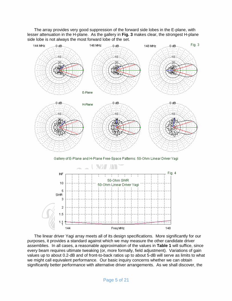
final questions will become whether or not the alternatives can sufficiently match the performance of the array that we are using as our standard. 2. The Low-Impedance Linear Driver Assembly: Before we tackle a true alternative to the linear driver, let’s perform a small set of modifications to our linear-driver Yagi to convert it into a low-impedance version. We need only shorten the spacing from the reflector to the driver, adjust the element lengths, and make a small change in the driver spacing to the first director. Fig. 5 shows a comparison of the general outlines of the 50-Ω and the low-impedance versions.

The exact dimensions for the model—in both wavelengths and inch terms—appear in Fig. 6. The low-impedance version uses a reflector that is slightly longer than the 50-Ω model reflector, but the new driver is nearly 1” shorter than the old one. The new driver requires a small increase in distance from the first director (about 1.6”), while the reflector is only 4” behind the driver, instead of more than 15”, as is the case for the 50-Ω Yagi. The boom length for the entire array is 230.3” (2.849 λ). Whether the 10” or 4% reduction in boom length justifies using a low impedance driving assembly might be subject to some debate, but not likely very much. The performance of the new version of the 12-element Yagi is very similar to the performance of the 50-Ω array, with the exception of the feedpoint impedance values. Table 2 provides the sampled data. Details vary across the band, but in general, the low-impedance version of the antenna shows close to the same gain, a deeper 180° dimple in the front-to-back pattern, and marginally better front-to-sidelobe performance. If the feedpoint impedance were not an issue—the important one for this discussion—one could not tell the difference by swapping one version of the antenna for the other one. Table 2. Performance of the 12-element Yagi with a low-impedance linear driver element Boom length = 2.849 λ or 230.3” at 146 MHz Category Frequency MHz 144 146 148 Gain dBi 14.30 14.87 14.86 Front-back ratio dB 19.46 35.21 23.61 E-fsl dB 21.38 22.40 26.09 E-BW degrees 36.0 34.2 32.9 H-fsl dB 17.15 18.19 16.73 H-BW degrees 39.2 37.2 35.6 Feedpoint R +/- jX Ω 7.39 – j13.55 12.81 – j0.30 17.68 + j6.45 12.8-Ω SWR 3.999 1.023 1.702

Page 7 of 21

The gallery of free-space E-plane and H-plane patterns in Fig. 7 confirms visually the impression left by the performance numbers. At 144 MHz, the E-plane pattern shows a slightly larger rearward fan of energy than the 50-Ω version, but likely nothing that some fine tuning of the elements cannot shrink. Otherwise, the two sets of patterns are almost interchangeable. The feedpoint impedance values are another matter entirely. The selection of the value at 146 MHz is not accidental in terms of the next step in the process. 12.8 Ω at resonance is about ¼ of the desired value for the folded-dipole driver. However, driver element reactance tends to sustain its rate of change as the resistive component decreases more rapidly. Hence, the 12.8-Ω SWR curve in Fig. 8 for the low-impedance array wholly fails to meet bandwidth requirements for a 2:1 ratio across the band. Note, however, that the rate of SWR increase is much higher below the design frequency than above it. By some judicious tweaking of the driver assembly element lengths and possibly the spacing values, we might extend the usable range. However, the center impedance value of 12.8 Ω is not especially desirable, even with a matching network. The greater the difference between the input and output impedances of a

Page 8 of 21

network, the more critical the tuning becomes. Therefore, we might not obtain full band coverage at the network junction value of 50 Ω.

Nevertheless, the low-impedance driver model does establish that the reflector and the driver have very small roles to play in determining the overall beam performance, especially when the array has 10 directors (and, of course, more in other possible Yagi designs).

Within the terms of our exercise, let us assume that we must maintain the shorter boom length of the low-impedance array. Further, let’s assume that we wish to maintain to the degree possible all of the pattern properties of the two arrays that we have so far reviewed. To achieve

Page 9 of 21

this goal, we need only replace the linear low-impedance driver with a suitably sized folded dipole. 3. The Folded-Dipole Driver Assembly: The folded-dipole driver will consist of the same 3/16”-diameter aluminum as all of the other elements in the array. We can construct a suitable element with 1” spacing between the long sections. When we insert it into the array, we discover that it fits almost perfectly with a length of 37.82”, a reduction from the 38.8” linear driver. The folded dipole will be shorter because the dual linear sections act much like a single fat element. The spacing from the first director is the same as for the linear low-impedance driver. We must move the reflector back 0.01-λ (about 0.8”) to achieve the same reflector-driver coupling that we obtained for the low-impedance assembly. Fig 9 provides the numerical information on the array dimensions.

Page 10 of 21

For comparison with both of the preceding Yagis, Table 3 samples the performance of the new array with its folded-dipole driver. Fig. 10 supplies the accompanying gallery of E-plane and H-plane free-space patterns. Table 3. Performance of the 12-element Yagi with a folded-dipole driver element Boom length = 2.859 λ or 231.1” at 146 MHz Category Frequency MHz 144 146 148 Gain dBi 14.47 14.93 14.89 Front-back ratio dB 21.25 37.38 23.83 E-fsl dB 21.43 22.54 26.12 E-BW degrees 35.8 34.2 32.9 H-fsl dB 16.27 17.73 16.40 H-BW degrees 39.2 37.1 35.7 Feedpoint R +/- jX Ω 41.57 – j30.77 64.57 – j6.15 79.88 + j15.08 12.8-Ω SWR 1.986 1.320 1.688

The similarities between the data for the first three Yagis should be striking. At the design frequency, the folded-dipole array manages a gain advantage over its low-impedance sibling of only 0.05-dB, a function of the electrical fattening of the driver element. The array very closely approaches almost all of the values achieved by the original longer 50-Ω Yagi. The H-plane patterns show a slight asymmetry of the minor lobes simply because the model places the

Page 11 of 21

upper long section of the driver 1” above the plane of directors and the reflector. The effect is insufficient to move the centerline of the main lobe by even 1°. In one arena, the folded dipole fails to match the original linear-driver 50-Ω design. Although the array achieve less than 2:1 SWR relative to 50 Ω across the entire band, as shown in Fig. 11, it does not match the exceeding low SWR values of the 240” array. The original beam used the driver in conjunction with the first director to form a driving system. The folded dipole does not present all of the conditions (without further model modification) to flatten its SWR curve to the same level. However, the folded dipole has been sized to move the minimum SWR point downward in the passband to allow an acceptable SWR value across the band.

Although the folded dipole matches the essential performance characteristics of the original linear driver version, it provides no advantages over the original 50-Ω array—with the possible exception of a 4% shortening of the boom. This result is wholly consistent with what we have learned about Yagi behavior over the decades, but does run contrary to a popular myth about such drivers. 4. The Quagi Driver Assembly: The quagi, as outlined in Fig. 1, consists of a normal Yagi set of directors, but employs quad loops for the driver and the reflector. As reasoning once went—before we had relatively easy methods of verification—since the quad loop has a gain advantage over the dipole, an advantage also shown by the 2-element driver reflector quad beam over the driver-reflector Yagi, we may apply these elements in a long-boom Yagi and obtain a similar gain advantage. Moreover, we may position these elements so that the 125-Ω impedance of the quad comes down to a natural 50-Ω for the Yagi assembly. It is possible to design quagis that work. Fig. 12 shows the modeled dimensions of a version that uses 3/16”-diameter elements throughout. The directors are identical to those for the other arrays, although the first director requires shortening to compensate for the increased coupling with the quad-loop driver. Most notable in the dimension chart is the fact that the quad-loop elements require much more space than required by the folded dipole and the 50-Ω linear-driver assembly. The driving quad loop is now about 4.6” behind the position of the original linear driver, while the reflector is about 19.5” behind that position. As a consequence, the quagi boom length is longer than the length of the original beam. At 244.1” (3.020 λ), it is the longest beam of the group.

Page 12 of 21

The quagi driver assembly spacing values are consistent with those of a 2-element quad beam that one might use independently. The required spacing between the reflector and the driver is about 0.18-λ, while a broadband quad beam would require a spacing value in the vicinity of 0.17-λ. Essentially, the quagi seems to confirm that we have placed a full quad beam behind a set of directors. For this exercise, we have retained the 10 directors used in all of the beams, modifying only the length of the first one in the set.

Page 13 of 21

To complete our interrogation of the quagi, we need the performance data in Table 4, as well as the gallery of free-space patterns in Fig. 13. The data may seem initially disappointing. To obtain coverage across the entire 2-meter band, the gain curve shows a descending set of values, in contrast to the mid-band peak values that the other arrays displayed. For this reason, I tend to find quagis used mostly for narrow-band applications, such as the first MHz of 2 meters or the small 1.25-meter band. The trend is in line with other quagi beams (using other director arrangements), but I cannot say whether judicious design work might correct this trait. Table 4. Performance of the 12-element Yagi with a quagi driver element Boom length = 3.020 λ or 244.1” at 146 MHz Category Frequency MHz 144 146 148 Gain dBi 14.55 14.09 12.84 Front-back ratio dB 21.77 24.04 17.41 E-fsl dB 19.87 28.46 15.43 E-BW degrees 33.4 31.8 31.6 H-fsl dB 13.50 11.98 10.12 H-BW degrees 37.2 35.5 35.9 Feedpoint R +/- jX Ω 44.88 – j32.96 57.78 + j2.29 75.15 + j32.28 12.8-Ω SWR 1.995 1.163 1.927

Even if we restrict our view to the lower half of the band, the quagi shows some tendencies that may be as significant as the gain curve. The side lobe suppression does not match any of

Page 14 of 21

the values reported for the other three arrays that we have examined. The H-plane is especially susceptible to strong sidelobes, although the E-plane values are well below those of the other beams. These phenomena have largely escaped attention because we tend to think of the quad loop—when fed at the center of one of its horizontal elements—as producing purely horizontal polarization. Unfortunately, this view of the quad loop is true in practice only up to a certain point—the point at which sidelobe development begins to become one of the important aspects of pattern formation. Fig. 14 provides a partial explanation of why the quagi shows stronger side lobes than the Yagis in which all elements form a single plane.

The current magnitude curves on the directors are completely normal and quite close to the values produced by all of the beams in this exercise. Only the quad loops differ in the element current distribution. For the driver and the reflector, the current magnitude goes to zero at the center of each side of the loop. The values rise until we reach a corner. The graphic shows a discontinuity at that point only because of the limitations of the method of display. The curves are continuous, and the smaller curves above the loops show only the peak values. The end values are not zero, but have the same magnitude as the tips of the visually horizontal “v” curves from the side sections of each loop. Each side section of the driver assembly loops represents a moderate current peak that is at right angles to the plane of the set of directors. In this orientation, the directors have very little influence of the patterns yielded by these currents. In the present design, the careful arrangement of directors to attenuate side lobes is ineffective, since the side-wire currents are cross polarized with respect to the directors. Since the side-wire currents do not reach peak element values, the resulting sidelobes are simply larger than those produced by all of the other beams. They are not necessarily fatal to the use of a quagi. However, for any application in which the strength of side lobes is significant, the quagi configuration might be the last choice among Yagi possibilities.

Page 15 of 21

Fig. 15 shows the SWR curve produced by the quagi driver section of the array. It fails to match the original 50-Ω linear-driver array. A single quad loop is a fairly broadband independent element. However, in the presence of parasitic elements, the quad shows very narrow-band tendencies. Even when designed for wide-band operation, the quad beam narrows its operating bandwidth as we add elements. Very often, the SWR curve is broader than the front-to-back curve, and neither is as wide as the ones that we can obtain from relatively standard modern Yagi designs. One might legitimately argue that the present test is somewhat unfair to quagi designs, largely because it employs a variable length director set, with too many directors for the boom length devoted to them. There are quagi designs that will show higher gain values at the center of the band, and they tend to use fewer directors with wider spacing. On the other hand, they also show even worse front-to-sidelobe ratio values, and even with much fatter elements (when measured as a fraction of a wavelength), worse SWR curves. Nothing in my collection of samples of quagi design in any way exceeds the performance values of the first three Yagis in this exercise for relatively equal boom lengths. Conclusion As the discussion of the quagi reveals, we can reach no absolute conclusions. Still, by equalizing the question of director arrangements, we were able to sample the alternatives to a linear driver assembly, especially the ones about which myths persist concerning performance improvements. The tests showed no improvement. In one case—the quagi—the test model did not match the performance of the other three candidates. Indeed, the indications appear to point in a single direction. Modern design has removed the need for an alternative element structure to achieve a direct 50-Ω feedpoint impedance. Moreover, the alternatives could not equal the flat SWR curve available from a linear driver assembly. More significantly, the alternative drivers could not exceed the performance of the array with the linear 50-Ω driver. Nonetheless, so long as we leave a crack in the door for the alternative designs to prove themselves, some folks will go one believing the old myths that have no foundation in extant designs.

Page 16 of 21

Appendix 1: A Comparison of Some Yagis and Quagis for 146 MHz

To provide an indication of the relative performance of Yagis and quagis, I have prepared the following table. It is somewhat of a fruit basket with apples, pears, and oranges. The apples are the OWA Yagis on shorter booms with a high front-to-sidelobe ratio. The pears are “normal” Yagis derived from 70-cm individually optimized designs by N6BV. I have altered the element diameter to 0.1875” to coincide with the OWA Yagis. Therefore, N6BV is in no way responsible for the performance values listed in the table, which might improve with specific 2-meter optimization. Both types of Yagis are broadband designs that cover all of 2-meters with a very low SWR.

The oranges are the quagis. The shorter quagis mostly come from sources lost over the years of storage in my model files. One exception is the design taken from The ARRL Antenna Book, Chapter 18, although the model required considerable modification to peak its performance. It uses AWG #12 quad loops and 1/8” linear directors. The 140” 7-element quagi uses AWG #14 wire, while the 132” version uses 0.25”-diameter elements. The remaining quagis are derived from scaled versions originating in a 220-MHz design by WB4WEN. I left the scaled wire diameter at 0.287”, and the gain values show the anticipated small improvement over (the Yagi) antennas with 0.1875”-diameter elements. See Table 5. Table 5. Free-space characteristics of Yagis and quagis by boom length at 146 MHz Boom Length Type/ No. of Gain Front-Back E-fsl E-BW Inches Feet Source Elements dBi Ratio dB dB degrees 113 9.4 Y-OWA 8 12.36 23.50 21.50 43.2 132 11.0 Q-unk 7 12.87 50.21 15.75 42.2 140 11.6 Q-unk 7 12.41 20.86 16.16 44.8 144 12.0 Y-OWA 9 13.01 21.90 30.42 41.2 153 12.8 Q-WEN 8 13.23 21.08 14.84 40.8 163 13.6 Q-unk 8 13.13 20.91 15.39 41.4 168 14.0 Y-BV 10 13.64 27.38 19.03 38.2 170 14.2 Q-AB 7 13.85 26.37 13.66 35.8 174 14.5 Y-OWA 10 13.49 22.40 23.56 39.6 179 14.9 Q-WEN 9 13.93 27.36 14.08 37.2 199 16.6 Y-BV 11 13.91 25.77 19.90 38.2 202 16.8 Q-WEN 10 14.33 23.13 13.71 35.2 205 17.1 Y-OWA 11 14.02 25.70 25.23 37.8 225 18.8 Q-WEN 11 14.70 21.39 12.92 33.4 234 19.5 Y-BV 12 14.72 31.16 16.98 34.6 249 20.8 Q-WEN 12 15.13 20.96 12.73 31.2 266 22.2 Y-BV 13 15.20 24.94 18.37 33.2 272 22.7 Q-WEN 13 15.35 19.29 12.09 30.0 296 24.7 Q-WEN 14 15.70 23.19 11.87 28.4 301 25.1 Y-BV 14 15.59 24.53 17.05 31.6 325 27.1 Q-WEN 15 16.01 23.66 11.52 27.2 328 27.3 Y-BV 15 15.98 23.73 15.23 29.6 369 30.8 Y-BV 16 16.55 26.63 16.61 28.0 Note: E-fsl = E-plane front-to-sidelobe ratio in dB; E-BW = E-plane beamwidth in degrees.

Page 17 of 21

Allowing for differences in element diameter, the table shows the increase of maximum forward gain as the boom length increases. The exceptions due to element size are small. The OWA Yagis show the largest front-to-sidelobe values, with the N6BV Yagis coming in second. The individual optimization of the N6BV Yagis results in slightly different element lengths and spacing values, since the series does not constitute a “trimming” series of Yagis, as would be the case with DL6WU designs. The WB4WEN quagi designs make use of equal length directors, except for the first, with some variability of spacing. Hence, to create the entries in the table, I trimmed one director at a time and re-optimized performance, mostly by adjusting the driver assembly loops and the first director. The WB4WEN design technique is one of two typically used in long-boom VHF and UHF all-loop beam designs, the other being a relatively constant and small taper in loop size as we move forward in the series of directors.

The quagis show consistently lower values of E-plane front-to-sidelobe ratio than either of the 2-types of Yagis. Of significance is the fact that lower front-to-sidelobe ratios are normally accompanied by smaller E-plane beamwidths. It appears that not all energy saved from the forward sidelobes shows up as increased gain. Rather, it serves also to broaden the beamwidth of the main lobe. The table is a further indicator, but not a final “proof,” that the quagi design does not offer significant gain advantages of Yagis with linear drivers when we track the gain on the basis of the overall boom length of a beam. The quagi driver assembly does require more boom space than the linear Yagi driver and reflector. Therefore, had we measured gain vs. the director set portion of the total boom length, we might obtain other results. For the average beam builder, the latter comparison would not make good sense, since a beam has a single overall boom. However, the exercise might be useful to basic theory of Yagi-vs.-quagi operation. Nevertheless, since a direct 50-Ω feedpoint impedance is easy to obtain in this century (and all of the listed beams are for direct connection to a 50-Ω feedline), the original impetus to construct a quagi has largely been supplanted by modern wide-band 50-Ω linear-element Yagi designs. Appendix 2: Quagi vs. Quad The WB4WEN quagi design played a major part in the listings in the first appendix. I noted in passing that the design technique is also used in beam designs using all quad-loop elements. That thought led to the question of what might happen if all of the linear directors disappeared, to be replaced by quad-loop directors. The test is virtually the inverse of the initial question with which we began our scan of Yagi driver assemblies. In July, 1972, J. Appel-Hansen published a report with the following conclusion: “experiments indicate that the gain of a Yagi-Uda antenna arrangement depends only upon the phase velocity of the surface wave traveling along the director array and not to any significant extent upon the particular forms of the director elements.” (“The Loop Antenna with Director Arrays of Loops and Rods,” IEEE Trans. Ant. and Prop, pp. 516 ff) The WB4WEN quagi gives us an opportunity to replicate Appel-Hansen’s experiment. The goal is to replace each director in the quagi—the 8-element version to keep matters simple—with a quad loop. The direct-element spacing will not change, although we might change the length of the forward loop or the length and spacing of the driver assembly elements to restore the feedpoint impedance. Fig. 16 shows the outlines of the two arrays. Fig. 17 provides—in EZNEC wire-table form—the quagi dimensions.

Page 18 of 21

The entire quagi array is 153” long. The forward-most director has been shortened to center the 50-Ω SWR curve. The first director is longer than the next 4 directors, all of which have a single length. The excess decimal places in the measurements result from the fact that this design is scaled to 146 from the 220-MHz band, at which the elements are 0.1875” in diameter. The dimensions for the corresponding quad beam appear in Fig. 18. To center the 50-Ω SWR, the forward-most director loop is shorter than the preceding loops and moved back 1”. The driver is slightly shorter, and the reflector moves forward 2”. Although one might disagree, I view these small adjustments as fair and within the normal ranges of final tweaking for any array. In short, the quad beam is only 3” shorter than the quagi and otherwise virtually identical to it.

Page 19 of 21

Table 6. Performance of the 8-element quagi and quad beams at 146 MHz Category Beam Type Quagi Quad Gain dBi 13.23 13.24 Front-back ratio dB 21.08 26.11 E-fsl dB 13.71 15.84 E-BW degrees 40.8 41.2 H-fsl dB 13.39 12.11 H-BW degrees 45.3 43.5 Feedpoint R +/- jX Ω 50.47 + j0.96 51.03 – j2.39 50-Ω SWR 1.022 1.053

Page 20 of 21

Table 6 lists the key performance categories for both arrays. The differences are all minuscule in terms of parasitic beam performance relative to boom length considerations. Indeed, one might be able to bring the two arrays into even closer alignment by careful tweaking of the dimensions. The general outcome is a confirmation of the Appel-Hansen results. Fig. 19 provides a gallery of free-space E-plane and H-plane patterns for further comparisons. Perhaps the only significant difference in the patterns is that the quad does a somewhat better job of attenuating the second rearward sidelobe in the H-plane especially.

As Fig. 20 shows, the 50-Ω SWR curves for the two arrays are very closely match, with the quad version having a slightly broader 2:1 SWR passband.

Page 21 of 21

A single exercise is not a proof, but only a suggestive indicator. Indeed, it is a confirmation case for the Appel-Hansen result that the shape of the directors matters very little, especially between linear rods and wire rings, so far as the forward gain of the parasitic array is concerned. Within the present context, the quad and the quagi are equivalent configurations for the design of a parasitic beam having certain performance characteristics. Since decisive confirmation requires many replications, one may replace the quad-loop driver assembly with various linear assemblies as a further test. From there one may move on to any number of other driver and director configurations. However, we may perhaps settle for mere suggestiveness in this already lengthy set of exercises.

© All Rights Reserved World Wide ANTENNEX LLC