Y + = (Y T Y) -1 Y T Y T Y is non-singular and squared ? (Full rank) Inversion is possible if: =Y...
85
Y + = (Y T Y) -1 Y T Y T Y is non-singular and squared ? (Full rank) Inversion is possible if: =Y Y + c c ˆ
-
date post
21-Dec-2015 -
Category
Documents
-
view
221 -
download
0
Transcript of Y + = (Y T Y) -1 Y T Y T Y is non-singular and squared ? (Full rank) Inversion is possible if: =Y...

Y+ = (YTY)-1 YT Y+ = (YTY)-1 YT
YTY is non-singular and squaredYTY is non-singular and squared??
(Full rank)(Full rank)
Inversion is possible if:Inversion is possible if:
=Y Y+c=Y Y+cc

Y’*Y is (33) but:
rank(Y’*Y)=2 !
rank(Y) = 2 =min(#r,#c)
=> Y is full rank
rank(Y) = 2 =min(#r,#c)
=> Y is full rank

Y should have:
#rows > #col.s
Y should have:
#rows > #col.s
11

Y should not be:
Rank deficient
Y should not be:
Rank deficient
22
Column are linearly dependentColumn are linearly dependent

!!

3 compon.s, 4 samples3 compon.s, 4 samples
4 wavel.s, 4 samples4 wavel.s, 4 samples
rank(x)=min(r(c),r(s))=3
rank(x) < min(# r, #c) =4
=> x is rank deficient

pinv can be performed when x is rank deficient..


pinv
?X= I (not square and singular X)?X= I (not square and singular X)
svd & estimation of X using significant factors
svd & estimation of X using significant factors
?U**V*T=I?U**V*T=I
V**-1U*TU**V*T=IV**-1U*TU**V*T=I
pseudo inversepseudo inverse
pinv(X)= X+ = V**-1U*Tpinv(X)= X+ = V**-1U*T
U*TU*=IU*TU*=I
*-1*=I*-1*=I
V*V*T=I ?V*V*T=I ?

ksks kCkC
XX
= CC+X= CC+XX
|| -X|||| -X||X
Criterion for fitting
ks
Criterion for fitting
ks
Hard Model
Hard Model
X
Projection of X onto space of C
X = C S classicX = C S classic
1. # samp.s ≥ # compon.s 2. C : full rank
(rank(C)= #compon.s) (lin indep conc profiles)
1. # samp.s ≥ # compon.s 2. C : full rank
(rank(C)= #compon.s) (lin indep conc profiles)

ksks kCkCXX
Hard Model
Hard Model
Projection of X onto space of C
C = X Z inverseC = X Z inverse
= XX+C= XX+CCC || -C|||| -C||C
Criterion for fitting
ks
Criterion for fitting
ks 1. # samp.s ≥ # wavel.s 2. X: full rank (rank(X)= # wavel.s)
- variab. Select. - Factor based methods
1. # samp.s ≥ # wavel.s 2. X: full rank (rank(X)= # wavel.s)
- variab. Select. - Factor based methods
!!!!

X is usually near to singular…
X is usually near to singular…
# samples < # wavel.s # wavel.s > # compon.s
# samples < # wavel.s # wavel.s > # compon.s

XX+XX+
=U**V*TV**-1U*T (signif factors)
=U***-1U*T
=TT+
=U**V*TV**-1U*T (signif factors)
=U***-1U*T
=TT+

ksks kCkC
XX
Hard Model
Hard Model
Projection of C onto space of T
C = T RZ inverseC = T RZ inverse
= TT+C= TT+CCC || -C|||| -C||C
Criterion for fitting
ks
Criterion for fitting
ks 1. # samp.s ≥ # PCs 2. T: full rank (lin indep col.s)
1. # samp.s ≥ # PCs 2. T: full rank (lin indep col.s)
SVDSVD
TT

ksks kCkC
XX
Hard Model
Hard Model
Projection of T onto space of C
T = C R classicT = C R classic
1. # samp.s ≥ # compon.s 2. C : full rank (lin indep.
conc prof.s)
1. # samp.s ≥ # compon.s 2. C : full rank (lin indep.
conc prof.s)
TTSVDSVD
T
= CC+T= CC+TT|| -T|||| -T||T
Criterion for fitting
k
Criterion for fitting
k

= CC+X= CC+XX
= XX+C= XX+CC
= CC+T= CC+TT
= TT+C= TT+CC pcrC (Target Transform)
pcrC (Target Transform)
ccrX (classical curve
resolution)
ccrX (classical curve
resolution)
pcrTpcrT
ccrCccrC
T J Thurston, R G Brereton Analyst 127, 2002, 659.T J Thurston, R G Brereton Analyst 127, 2002, 659.

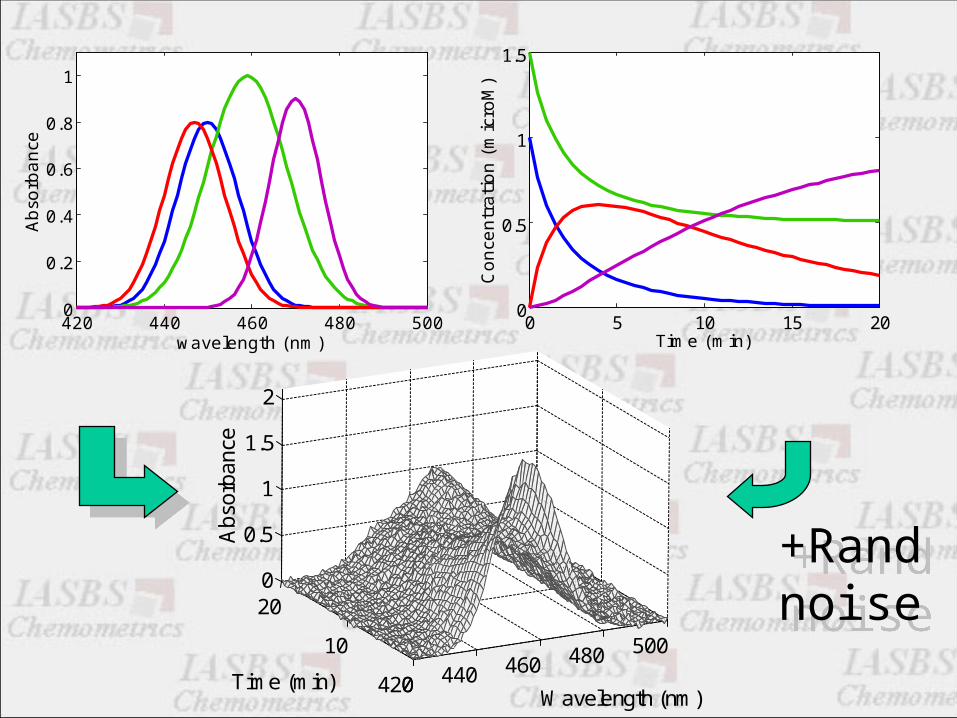
The considered kinetic system:The considered kinetic system:
Second order consecutiveSecond order consecutive
0 5 10 15 200
0.5
1
1.5
Time (min)
Conce
ntr
ati
on (
mic
roM
)
A+B CDA+B CD
Spectral meas. In 101 wavel.s each 30 sec (41 times)
Spectral meas. In 101 wavel.s each 30 sec (41 times)
r(C)=3# indep react.s +1
r(C)=3# indep react.s +1
420 440 460 480 500
0
10
200
0.5
1
1.5
2
Wavelength (nm)Time (min)
Abs
orba
nce

ccrC:ccrC:
X1=[X(:,50) X(:,70) X(:,90)]X1=[X(:,50) X(:,70) X(:,90)]
=X1*inv(X1‘*X1)*X1'*C=X1*inv(X1‘*X1)*X1'*CC
=X*inv(X‘*X)*X'*C=X*inv(X‘*X)*X'*CC 11
=X*pinv(X)*C=X*pinv(X)*CC
X(41x101) 41 samples r(X)=3 101 wavel.s
X(41x101) 41 samples r(X)=3 101 wavel.s
1 # samp.s ≥ # wavel.s 2 rank(X)= # wavel.s
1 # samp.s ≥ # wavel.s 2 rank(X)= # wavel.s
Information content !
Information content !

ccrX:
=C*inv(C’*C)*C’*X=C*inv(C’*C)*C’*XX C1=C(:,2:4)C1=C(:,2:4)
=C1*inv(C1’*C1)*C1’*X=C1*inv(C1’*C1)*C1’*X
=C*pinv(C)*X=C*pinv(C)*X X
X
1. # samp.s ≥ # compon.s 2. rank(C)= #compon.s
1. # samp.s ≥ # compon.s 2. rank(C)= #compon.s
C(41x4) 41 samples r(X)=3 4 compon.s

pcrT:pcrT:
=C*inv(C’*C)*C’*T=C*inv(C’*C)*C’*TT C1=C(:,2:4)C1=C(:,2:4)
=C1*inv(C1’*C1)*C1’*T=C1*inv(C1’*C1)*C1’*TT
=C*pinv(C)*T=C*pinv(C)*TT

pcrC:pcrC:
=T*T’*C=T*T’*CC
1. # samp.s ≥ # PCs 2. rank(T)= # col.s (always it is so…)
1. # samp.s ≥ # PCs 2. rank(T)= # col.s (always it is so…)

Overlap effectOverlap effect

420 440 460 480 5000
0.2
0.4
0.6
0.8
1
wavelength (nm)
Abso
rbance
0 5 10 15 200
0.5
1
1.5
Time (min)
Conce
ntr
ati
on (
mic
roM
)
420 440 460 480 500
0
10
200
0.5
1
1.5
2
Wavelength (nm)Time (min)
Abs
orba
nce
+Rand noise
+Rand noise

0.36 0.38 0.4 0.42 0.440.09
0.095
0.1
0.105
0.11ccrX
noise 0.02
k1
k2
0.3 0.35 0.4 0.45 0.5
0.08
0.09
0.1
0.11
0.12 ccrCnoise 0.02
k1
k2
0.36 0.38 0.4 0.42 0.440.09
0.095
0.1
0.105
0.11pcrT
noise 0.02
k1
k2
0.3 0.35 0.4 0.45 0.5
0.08
0.09
0.1
0.11
0.12 pcrCnoise 0.02
k1
k2

Spectral overlap (in the presence of some noise) results in some deviation in the results
from
***C
methods
Spectral overlap (in the presence of some noise) results in some deviation in the results
from
***C
methods

Results from application of ***C and ***X methods
are different …
Results from application of ***C and ***X methods
are different …
One way to obtain more similar results from ***C and ***X methods are application of
constraints
One way to obtain more similar results from ***C and ***X methods are application of
constraints

Presence of
heteroscedastic noise

+ a heterosced. noise
+ a heterosced. noise
41 reaction times &101 wavelengths
41 reaction times &101 wavelengths
050
100020
400
0.5
1
1.5
2
reaction timeVariable No.
Ab
sorb
ance
0 20 40 60 80 100-0.015
-0.01
-0.005
0
0.005
0.01
0.015
Variable No.
Ab
so
rban
ce

0.36 0.38 0.4 0.42 0.440.094
0.096
0.098
0.1
0.102
0.104
0.106
k1
k2
Inaccurate results from ccrX !Inaccurate results from ccrX !

0 20 40 60 80 100-0.05
0
0.05
Variable No.
Ab
sorb
ance weightsweights
weighted regression…weighted regression…
||W ( -X)||||W ( -X)||X

1/SD1
1/SD2
…
1/SDn
W =W =

Accurate results from weighted ccrX !
Accurate results from weighted ccrX !
0.3995 0.4 0.40050.0995
0.1
0.1005
k1
k2
n=50n=50

FSMWFA in daset 6
-7.5
-5.5
-3.5
-1.5
0.5
2.5
300 320 340 360 380 400 420 440 460 480 500
wavelength
log
(eig
valu
e)
Recognition of the presence of heterosc. noise
Recognition of the presence of heterosc. noise
FSMWFA

0 10 20 30 400.99
0.995
1
1.005
1.01
Sample number
Sam
plin
g er
ror
coef
ficie
nt
0
5
100 10 20 30 40 50
0.99
0.995
1
1.005
1.01
1.015
Non-random sampling error
Non-random sampling error
A more serious source
of error
A more serious source
of error
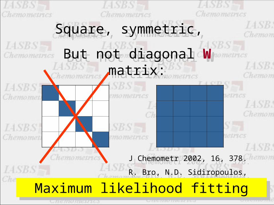
Square, symmetric,
But not diagonal W matrix:
Square, symmetric,
But not diagonal W matrix:
J Chemometr 2002, 16, 378.
R. Bro, N.D. Sidiropoulos, A.K. Smilde
J Chemometr 2002, 16, 378.
R. Bro, N.D. Sidiropoulos, A.K. Smilde
Maximum likelihood fittingMaximum likelihood fitting

Presence of non-random sampling error nS=0.005
Presence of non-random sampling error nS=0.005
0.3 0.4 0.5 0.6
0.075
0.08
0.085
0.09
0.095
0.1
0.105
k1
k2
|| -X|||| -X||X ||W ( -X)||||W ( -X)||X
0.3 0.4 0.5 0.6
0.075
0.08
0.085
0.09
0.095
0.1
0.105
k1
k2
Weighted regression
Weighted regression
ccrXccrX
J Chemom 2002, 16,387. R.Bro et alJ Chemom 2002, 16,387. R.Bro et al
Presence of unknown interference

Changing interference, drift , or shiftChanging interference, drift , or shift
400 420 440 460 480 5000
0.2
0.4
0.6
0.8
1
1.2
1.4
absorbance of pure components
wavelength (nm)
abso
rban
ce
400 420 440 460 480 5000
0.2
0.4
0.6
0.8
1
1.2
1.4
absorbance of pure components
wavelength (nm)
abso
rban
ce
0 5 10 15 200
0.5
1
1.5
concentration profiles
reaction time(min)
con
cen
trat
ion
(m
icro
M)
0 5 10 15 200
0.5
1
1.5
concentration profiles
reaction time(min)
con
cen
trat
ion
(m
icro
M)
400 420 440 460 480 5000
0.5
1
1.5
2
2.5
Data
Wavelength (nm)
Ab
sorb
ance
rank(Data)=4rank(Data)=4

0.38 0.385 0.39 0.395 0.4 0.4050.095
0.1
0.105
0.11
0.115
0.12
0.125
0.13
k1
k2
pcrTpcrT
0.39 0.395 0.4 0.4050.097
0.098
0.099
0.1
0.101
0.102
k1
k2
pcrCpcrC
0.385 0.39 0.395 0.4 0.4050.099
0.1
0.101
0.102
0.103
k1
k2
ccrXccrX
0.39 0.395 0.4 0.4050.097
0.098
0.099
0.1
0.101
0.102
0.103
k1
k2
ccrCccrC

Presence of shift or drift (a changing interference) results in
serious deviations in
***X
Methods
(but not in ***C methods)
Presence of shift or drift (a changing interference) results in
serious deviations in
***X
Methods
(but not in ***C methods)
Why?Why?

= CC+X= CC+XX = XX+C= XX+CC= CC+T= CC+TT
In the presence of shift, drift or changing interferences:
T or X space includes 1. the concentration changes according to the model 2. variations from shift, drift or
changing interference
C space includes only the concentration changes according to the model
In the presence of shift, drift or changing interferences:
T or X space includes 1. the concentration changes according to the model 2. variations from shift, drift or
changing interference
C space includes only the concentration changes according to the model
Projection of a larger space to a smaller one
Projection of a larger space to a smaller one
Projection of a smaller space to a larger one
Projection of a smaller space to a larger one
= TT+C= TT+CC

= TT+C= TT+CC
in the presence of unknown interference, drift or shift.
Target Transform (pcrC) is the most preferred method

Constant interferenceConstant interference
400 420 440 460 480 5000
0.2
0.4
0.6
0.8
1
1.2
1.4absorbance of pure components
wavelength (nm)
abso
rban
ce
400 420 440 460 480 5000
0.2
0.4
0.6
0.8
1
1.2
1.4absorbance of pure components
wavelength (nm)
abso
rban
ce
0 5 10 15 200
0.5
1
1.5
concentration profiles
reaction time(min)
con
cen
trat
ion
(m
icro
M)
0 5 10 15 200
0.5
1
1.5
concentration profiles
reaction time(min)
con
cen
trat
ion
(m
icro
M)
400 420 440 460 480 5000
0.5
1
1.5
2
2.5
Data
Wavelength (nm)
Ab
sorb
ance
rank(Data)=3 !rank(Data)=3 !
A+B CDA+B CD

0.399 0.3995 0.4 0.4005 0.4010.099
0.0995
0.1
0.1005
0.101
k1
k2
0.399 0.3995 0.4 0.4005 0.4010.099
0.0995
0.1
0.1005
0.101
k1
k2
ccrCccrC
0.399 0.3995 0.4 0.4005 0.4010.099
0.0995
0.1
0.1005
0.101
k1
k2
ccrXccrX
0.399 0.3995 0.4 0.4005 0.4010.099
0.0995
0.1
0.1005
0.101
k1
k2
pcrTpcrT
0.399 0.3995 0.4 0.4005 0.4010.099
0.0995
0.1
0.1005
0.101
k1
k2pcrCpcrC

A constant interference does not show any significant effect the
accuracy of ***X and ***C methods.
A constant interference does not show any significant effect the
accuracy of ***X and ***C methods.

Target test fittingTarget test fitting
From:
J Chemometr. 2001, 15, 511.
P.Jandanklang, M. Maeder, A. C. whitson
From:
J Chemometr. 2001, 15, 511.
P.Jandanklang, M. Maeder, A. C. whitson
-0.1 -0.05 0 0.05 0.10
5
10
15
20
25
30
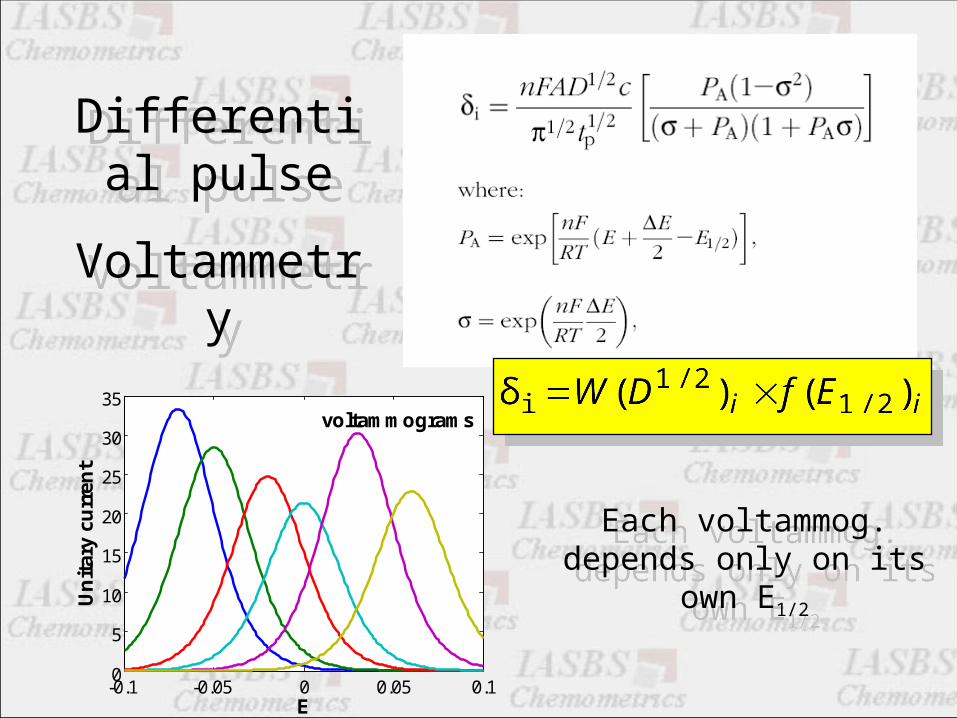
35voltammograms
E
Un
itar
y cu
rren
t
Differential pulse
Voltammetry
Differential pulse
Voltammetry
Each voltammog. depends only on its own E1/2
Each voltammog. depends only on its own E1/2

3
2
3
2
MLLM
MLLM
MLLM
33
22
]][[
][
]][[
][
]][[
][
3
2
LM
ML
LM
ML
LM
ML
ML
ML
ML
Successive complexation:

0....))1((][)(][][ 211
11
TLnTLTMn
nnTLTMn
nn
n CCCnLCCLL
)][....][][1(
][][
)][....][][1(
1][
221
221
nn
nn
n
nn
LLL
LML
LLLM
nn
n LM
ML
LM
ML
]][[
][,.....,
]][[
][1
][....][][
][....][][
nTL
nTM
MLnMLLC
MLMLMC
Analyst , 2001 , 126 , 371-377Each concn. profile includes 1,…, n
Each concn. profile includes 1,…, n

0 20 40 60 800
0.2
0.4
0.6
0.8
1
Ctotal L
Cu
rren
t m
icro
A
-0.1 -0.05 0 0.05 0.10
5
10
15
20
25
30
35voltammograms
E
Un
itar
y cu
rren
t
-0.1 -0.05 0 0.05 0.10
5
10
15
20
25
30
35
Data
E
curr
ent
X

X=CSX=CS
X=UVT=TVX=UVT=TV
= VVT s= VVT s
= UUT c = TTT c= UUT c = TTT c
s
c
voltammogrvoltammogr
concn.concn.

For estimation of concn. profiles 1,…,n
(n parameters) should be optimized
simultaneously
For estimation of concn. profiles 1,…,n
(n parameters) should be optimized
simultaneously
1,…,n are dependent parameters
1,…,n are dependent parameters

Simultaneous optimization of n dependent nonlinear
parameters:
Simultaneous optimization of n dependent nonlinear
parameters:
• Simplex method.
• Levenberg-Marquardt
•…
• Simplex method.
• Levenberg-Marquardt
•…

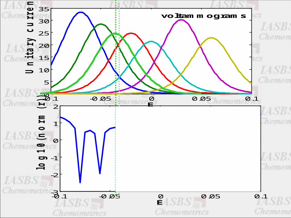
estimation of
(E1/2)1, …, (E1/2 )n
values for voltammograms
estimation of
(E1/2)1, …, (E1/2 )n
values for voltammograms
(E1/2)1, …, (E1/2 )n
are independent parameters
(E1/2)1, …, (E1/2 )n
are independent parameters

-0.1 -0.05 0 0.05 0.1-3
-2
-1
0
1
2
E
log
10(n
orm
(r))-0.1 -0.05 0 0.05 0.1
0
5
10
15
20
25
30
35voltammograms
E
Un
itary c
urren
t

-0.1 -0.05 0 0.05 0.1-3
-2
-1
0
1
2
E
log
10(n
orm
(r))-0.1 -0.05 0 0.05 0.1
0
5
10
15
20
25
30
35voltammograms
E
Un
itary c
urren
t

-0.1 -0.05 0 0.05 0.1-3
-2
-1
0
1
2
E
log
10(n
orm
(r))-0.1 -0.05 0 0.05 0.1
0
5
10
15
20
25
30
35voltammograms
E
Un
itary c
urren
t

-0.1 -0.05 0 0.05 0.1-3
-2
-1
0
1
2
E
log
10(n
orm
(r))-0.1 -0.05 0 0.05 0.1
0
5
10
15
20
25
30
35voltammograms
E
Un
itary c
urren
t

-0.1 -0.05 0 0.05 0.1-3
-2
-1
0
1
2
E
log
10(n
orm
(r))-0.1 -0.05 0 0.05 0.1
0
5
10
15
20
25
30
35voltammograms
E
Un
itary c
urren
t
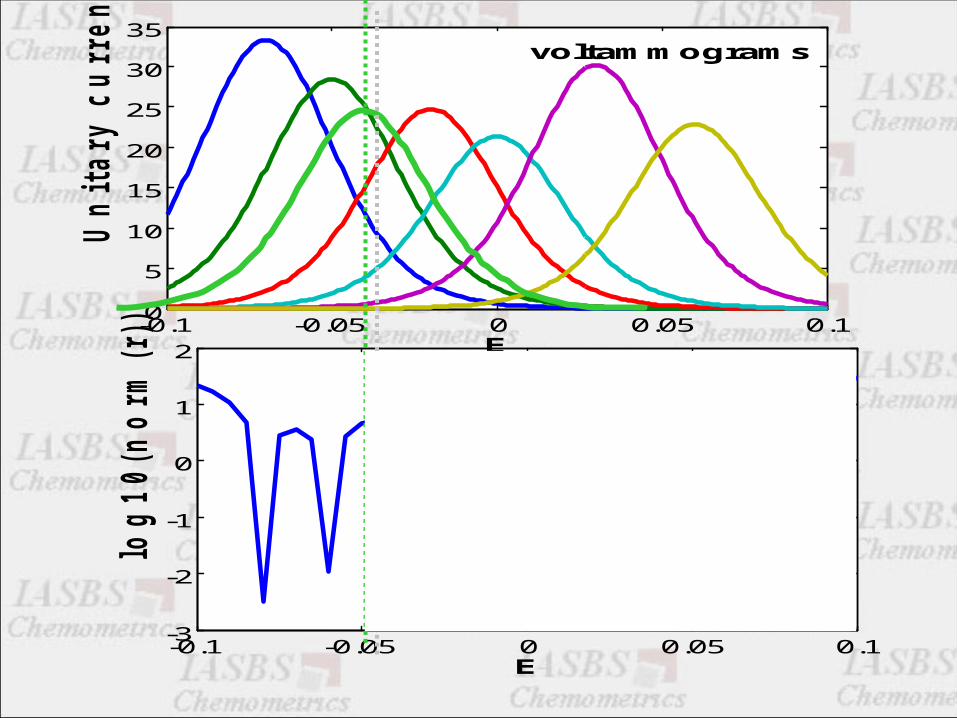
r = || - s|| 0s
(E1/2)M(E1/2)M

-0.1 -0.05 0 0.05 0.1-3
-2
-1
0
1
2
E
log
10(n
orm
(r))-0.1 -0.05 0 0.05 0.1
0
5
10
15
20
25
30
35voltammograms
E
Un
itary c
urren
t

-0.1 -0.05 0 0.05 0.1-3
-2
-1
0
1
2
E
log
10(n
orm
(r))-0.1 -0.05 0 0.05 0.1
0
5
10
15
20
25
30
35voltammograms
E
Un
itary c
urren
t

-0.1 -0.05 0 0.05 0.1-3
-2
-1
0
1
2
E
log
10(n
orm
(r))-0.1 -0.05 0 0.05 0.1
0
5
10
15
20
25
30
35voltammograms
E
Un
itary c
urren
t

-0.1 -0.05 0 0.05 0.1-3
-2
-1
0
1
2
E
log
10(n
orm
(r))-0.1 -0.05 0 0.05 0.1
0
5
10
15
20
25
30
35voltammograms
E
Un
itary c
urren
t

-0.1 -0.05 0 0.05 0.1-3
-2
-1
0
1
2
E
log
10(n
orm
(r))-0.1 -0.05 0 0.05 0.1
0
5
10
15
20
25
30
35voltammograms
E
Un
itary c
urren
t
r = || - s|| 0s
(E1/2)M(E1/2)M
(E1/2)ML(E1/2)ML

-0.1 -0.05 0 0.05 0.1-3
-2
-1
0
1
2
E
log
10(n
orm
(r))-0.1 -0.05 0 0.05 0.1
0
5
10
15
20
25
30
35voltammograms
E
Un
itary c
urren
t
-0.1 -0.05 0 0.05 0.1-3
-2
-1
0
1
2
E
log
10(n
orm
(r))-0.1 -0.05 0 0.05 0.1
0
5
10
15
20
25
30
35voltammograms
E
Un
itary c
urren
t
-0.1 -0.05 0 0.05 0.1-3
-2
-1
0
1
2
E
log
10(n
orm
(r))-0.1 -0.05 0 0.05 0.1
0
5
10
15
20
25
30
35voltammograms
E
Un
itary c
urren
t

-0.1 -0.05 0 0.05 0.1-3
-2
-1
0
1
2
E
log
10(n
orm
(r))-0.1 -0.05 0 0.05 0.1
0
5
10
15
20
25
30
35voltammograms
E
Un
itary c
urren
t

-0.1 -0.05 0 0.05 0.1-3
-2
-1
0
1
2
E
log
10(n
orm
(r))-0.1 -0.05 0 0.05 0.1
0
5
10
15
20
25
30
35voltammograms
E
Un
itary c
urren
t

-0.1 -0.05 0 0.05 0.1-3
-2
-1
0
1
2
E
log
10(n
orm
(r))-0.1 -0.05 0 0.05 0.1
0
5
10
15
20
25
30
35voltammograms
E
Un
itary c
urren
t
r = || - s|| 0s
(E1/2)M(E1/2)M (E1/2)ML2
(E1/2)ML2(E1/2)ML
(E1/2)ML

-0.1 -0.05 0 0.05 0.1-3
-2
-1
0
1
2
E
log
10(n
orm
(r))-0.1 -0.05 0 0.05 0.1
0
5
10
15
20
25
30
35voltammograms
E
Un
itary c
urren
t

-0.1 -0.05 0 0.05 0.1-3
-2
-1
0
1
2
E
log
10(n
orm
(r))-0.1 -0.05 0 0.05 0.1
0
5
10
15
20
25
30
35voltammograms
E
Un
itary c
urren
t
-0.1 -0.05 0 0.05 0.1-3
-2
-1
0
1
2
E
log
10(n
orm
(r))-0.1 -0.05 0 0.05 0.1
0
5
10
15
20
25
30
35voltammograms
E
Un
itary c
urren
t
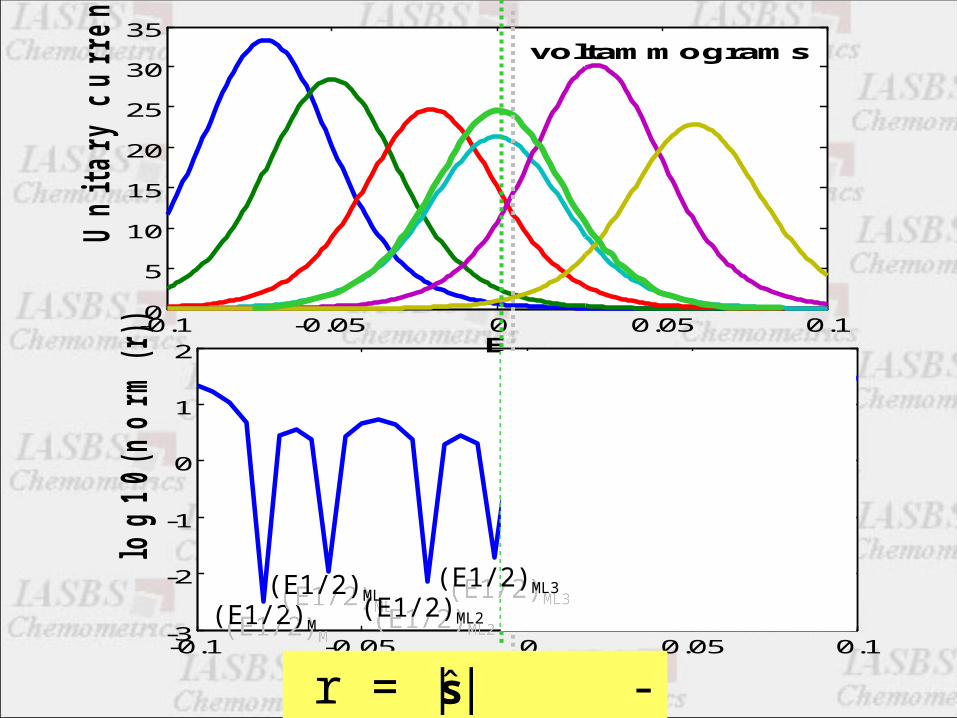
r = || - s|| 0s
(E1/2)M(E1/2)M
(E1/2)ML(E1/2)ML
(E1/2)ML2(E1/2)ML2
(E1/2)ML3(E1/2)ML3

-0.1 -0.05 0 0.05 0.1-3
-2
-1
0
1
2
E
log
10(n
orm
(r))-0.1 -0.05 0 0.05 0.1
0
5
10
15
20
25
30
35voltammograms
E
Un
itary c
urren
t

-0.1 -0.05 0 0.05 0.1-3
-2
-1
0
1
2
E
log
10(n
orm
(r))-0.1 -0.05 0 0.05 0.1
0
5
10
15
20
25
30
35voltammograms
E
Un
itary c
urren
t

-0.1 -0.05 0 0.05 0.1-3
-2
-1
0
1
2
E
log
10(n
orm
(r))-0.1 -0.05 0 0.05 0.1
0
5
10
15
20
25
30
35voltammograms
E
Un
itary c
urren
t
r = || - s|| 0s
(E1/2)M(E1/2)M
(E1/2)ML(E1/2)ML
(E1/2)ML2(E1/2)ML2
(E1/2)ML3(E1/2)ML3
(E1/2)L(E1/2)L

-0.1 -0.05 0 0.05 0.1-3
-2
-1
0
1
2
E
log
10(n
orm
(r))-0.1 -0.05 0 0.05 0.1
0
5
10
15
20
25
30
35voltammograms
E
Un
itary c
urren
t

-0.1 -0.05 0 0.05 0.1-3
-2
-1
0
1
2
E
log
10(n
orm
(r))-0.1 -0.05 0 0.05 0.1
0
5
10
15
20
25
30
35voltammograms
E
Un
itary c
urren
t

-0.1 -0.05 0 0.05 0.1-3
-2
-1
0
1
2
E
log
10(n
orm
(r))-0.1 -0.05 0 0.05 0.1
0
5
10
15
20
25
30
35voltammograms
E
Un
itary c
urren
t
r = || - s|| 0s
(E1/2)M(E1/2)M
(E1/2)ML(E1/2)ML
(E1/2)ML2(E1/2)ML2
(E1/2)ML3(E1/2)ML3
(E1/2)L(E1/2)L
(E1/2)I(E1/2)I

-0.1 -0.05 0 0.05 0.1-3
-2
-1
0
1
2
E
log
10(n
orm
(r))-0.1 -0.05 0 0.05 0.1
0
5
10
15
20
25
30
35voltammograms
E
Un
itary c
urren
t

Optimum values for
n independent parameters can be estimated
by
grid search of one parameter.
Optimum values for
n independent parameters can be estimated
by
grid search of one parameter.

A difficult aspect of hard modeling is determination of correct model

Thanks.Thanks.
Thanks to:
Miss Maryam Khoshkam
and
Mr Yaser Beyad
for a number of m-files and slides.
Thanks to:
Miss Maryam Khoshkam
and
Mr Yaser Beyad
for a number of m-files and slides.