P, NP, and NP-Completeness:The Basics of Computational ComplexityOded GoldreichDepartment of Computer Science and Applied MathematicsWeizmann Institute of Science, Rehovot, Israel.June 14, 2008

Ito Dana

c Copyright 2008 by Oded Goldreich.Permission to make copies of part or all of this work for personal or classroom use isgranted without fee provided that copies are not made or distributed for pro�t or com-mercial advantage and that new copies bear this notice and the full citation on the �rstpage. Abstracting with credit is permitted.

II

PrefaceThe strive for e�ciency is ancient and universal, as time and other resources arealways in shortage. Thus, the question of which tasks can be performed e�cientlyis central to the human experience.A key step towards the systematic study of the aforementioned question is arigorous de�nition of the notion of a task and of procedures for solving tasks. Thesede�nitions were provided by computability theory, which emerged in the 1930's.This theory focuses on computational tasks, and considers automated procedures(i.e., computing devices and algorithms) that may solve such tasks.In focusing attention on computational tasks and algorithms, computabilitytheory has set the stage for the study of the computational resources (like time) thatare required by such algorithms. When this study focuses on the resources that arenecessary for any algorithm that solves a particular task (or a task of a particulartype), the study becomes part of the theory of Computational Complexity (alsoknown as Complexity Theory).1Complexity Theory is a central �eld of the theoretical foundations of ComputerScience. It is concerned with the study of the intrinsic complexity of computationaltasks. That is, a typical Complexity theoretic study refers to the computationalresources required to solve a computational task (or a class of such tasks), ratherthan referring to a speci�c algorithm or an algorithmic schema. Actually, researchin Complexity Theory tends to start with and focus on the computational resourcesthemselves, and addresses the e�ect of limiting these resources on the class oftasks that can be solved. Thus, Computational Complexity is the general studyof the what can be achieved within limited time (and/or other limited naturalcomputational resources).The most famous question of complexity theory is the P-vs-NP Question, andthe current book is focused on it. The P-vs-NP Question can be phrased as askingwhether or not �nding solutions is harder than checking the correctness of solu-tions. An alternative formulation asks whether or not discovering proofs is harderthan verifying their correctness; that is, is proving harder than verifying. The fun-1In contrast, when the focus is on the design and analysis of speci�c algorithms (rather thanon the intrinsic complexity of the task), the study becomes part of a related sub�eld that maybe called Algorithmic Design and Analysis. Furthermore, Algorithmic Design and Analysis tendsto be sub-divided according to the domain of mathematics, science and engineering in which thecomputational tasks arise. In contrast, Complexity Theory typically maintains a unity of thestudy of tasks solvable within certain resources (regardless of the origins of these tasks).III

IVdamental nature of this question is evident in each of these formulations, whichare in fact equivalent. It is widely believed that the answer to these equivalent for-mulations is that �nding (resp., proving) is harder than checking (resp., verifying);that is, it is believed that P is di�erent from NP.At present, when faced with a seemingly hard problem in NP, we can onlyhope to prove that it is not in P assuming that NP is di�erent from P. This iswhere the theory of NP-completeness, which is based on the notion of an e�cientreduction, comes into the picture. In general, one computational problem is (e�-ciently) reducible to another problem if it is possible to (e�ciently) solve the formerwhen provided with an (e�cient) algorithm for solving the latter. A problem (inNP) is NP-complete if any problem in NP is e�ciently reducible to it. Amazinglyenough, NP-complete problems exist, and furthermore hundreds of natural compu-tational problems arising in many di�erent areas of mathematics and science areNP-complete.The main focus of the current book is on the P-vs-NP Question and the theoryof NP-completeness. Additional topics that are covered include the treatmentof the general notion of an e�cient reduction between computational problems,which provides a tighter relation between the aforementioned search and decisionproblems. The book also provides adequate preliminaries regarding computationalproblems and computational models.Relation to a di�erent book of the author. The current book is a revision ofChapter 2 and Section 1.2 of the author's book Computational Complexity: A Con-ceptual Perspective [13]. The revision was aimed at making the book more friendlyto the novice. In particular, several proofs were further detailed and numerousexercises were added.Web-site for notices regarding this book. We intend to maintain a web-sitelisting corrections of various types. The location of the site ishttp://www.wisdom.weizmann.ac.il/�oded/bc-book.html

OverviewThis book starts by providing the relevant background on computability theory,which is the setting in which complexity theoretic questions are being studied.Most importantly, this preliminary chapter (i.e., Chapter 1) provides a treatmentof central notions such as search and decision problems, algorithms that solvesuch problems, and their complexity. Special attention is given to the notion of auniversal algorithm.The main part of this book (i.e., Chapters 2{5) is focused on the P-vs-NPQuestion and on the theory of NP-completeness. Additional topics covered in thispart include the general notion of an e�cient reduction (with a special emphasison self-reducibility), the existence of problems in NP that are neither NP-completenor in P, the class coNP, optimal search algorithms, and promise problems. A briefoverview of this main part follows.Loosely speaking, the P-vs-NP Question refers to search problems for which thecorrectness of solutions can be e�ciently checked (i.e., there is an e�cient algorithmthat given a solution to a given instance determines whether or not the solutionis correct). Such search problems correspond to the class NP, and the question iswhether or not all these search problems can be solved e�ciently (i.e., is there ane�cient algorithm that given an instance �nds a correct solution). Thus, the P-vs-NP Question can be phrased as asking whether or not �nding solutions is harderthan checking the correctness of solutions.An alternative formulation, in terms of decision problems, refers to assertionsthat have e�ciently veri�able proofs (of relatively short length). Such sets ofassertions correspond to the class NP, and the question is whether or not proofsfor such assertions can be found e�ciently (i.e., is there an e�cient algorithm thatgiven an assertion determines its validity and/or �nds a proof for its validity).Thus, the P-vs-NP Question can be phrased as asking whether or not discoveringproofs is harder than verifying their correctness; that is, is proving harder thanverifying (or are proofs valuable at all).Indeed, it is widely believed that the answer to the two equivalent formulationsis that �nding (resp., discovering) is harder than checking (resp., verifying); thatis, that P is di�erent than NP. The fact that this natural conjecture is unsettledseems to be one of the big sources of frustration of complexity theory. The author'sopinion, however, is that this feeling of frustration is out of place. In any case, atpresent, when faced with a seemingly hard problem in NP, we cannot expect toV

VIprove that the problem is not in P (unconditionally). The best we can expect is aconditional proof that the said problem is not in P, based on the assumption thatNP is di�erent from P. The contrapositive is proving that if the said problem is inP, then so is any problem in NP (i.e., NP equals P). This is where the theory ofNP-completeness comes into the picture.The theory of NP-completeness is based on the notion of an e�cient reduction,which is a relation between computational problems. Loosely speaking, one com-putational problem is e�ciently reducible to another problem if it is possible toe�ciently solve the former when provided with an (e�cient) algorithm for solvingthe latter. Thus, the �rst problem is not harder to solve than the second one. Aproblem (in NP) is NP-complete if any problem in NP is e�ciently reducible toit. Thus, the fate of the entire class NP (with respect to inclusion in P) rests witheach individual NP-complete problem. In particular, showing that a problem isNP-complete implies that this problem is not in P unless NP equals P. Amazinglyenough, NP-complete problems exist, and furthermore hundreds of natural compu-tational problems arising in many di�erent areas of mathematics and science areNP-complete.The foregoing paragraphs refer to material that is covered in Chapters 2-4.Speci�cally, Chapter 2 is devoted to the P-vs-NP Question per se, Chapter 3 isdevoted to the notion of an e�cient reduction, and Chapter 4 is devoted to thetheory of NP-completeness. We mention that that NP-complete problems are notthe only seemingly hard problems in NP; that is, if P is di�erent than NP, then NPcontains problems that are neither NP-complete nor in P (see Section 4.4).Additional related topics are discussed in Chapter 5. In particular, in Sec-tion 5.2, it is shown that the P-vs-NP Question is not about inventing sophisticatedalgorithms or ruling out their existence, but rather boils down to the analysis ofa single known algorithm; that is, we will present an optimal search algorithm forany problem in NP, while having not clue about its time-complexity.The book also includes a brief overview of complexity theory (see Epilogue) anda laconic review of some popular computational problems (see Appendix).

To the TeacherAccording to a common opinion, the most important aspect of a scienti�c workis the technical result that it achieves, whereas explanations and motivations aremerely redundancy introduced for the sake of \error correction" and/or comfort. Itis further believed that, like in a work of art, the interpretation of the work shouldbe left with the reader.The author strongly disagrees with the aforementioned opinions, and arguesthat there is a fundamental di�erence between art and science, and that this dif-ference refers exactly to the meaning of a piece of work. Science is concerned withmeaning (and not with form), and in its quest for truth and/or understanding sci-ence follows philosophy (and not art). The author holds the opinion that the mostimportant aspects of a scienti�c work are the intuitive question that it addresses,the reason that it addresses this question, the way it phrases the question, the ap-proach that underlies its answer, and the ideas that are embedded in the answer.Following this view, it is important to communicate these aspects of the work.The foregoing issues are even more acute when it comes to complexity theory,�rstly because conceptual considerations seems to play an even more central rolein complexity theory (than in other scienti�c �elds). Secondly (and even moreimportantly), complexity theory is extremely rich in conceptual content. Thus,communicating this content is of primary importance, and failing to do so missesthe most important aspects of complexity theory.Unfortunately, the conceptual content of complexity theory is rarely communi-cated (explicitly) in books and/or surveys of the area. The annoying (and quiteamazing) consequences are students that have only a vague understanding of themeaning and general relevance of the fundamental notions and results that theywere taught. The author's view is that these consequences are easy to avoid by tak-ing the time to explicitly discuss the meaning of de�nitions and results. A closelyrelated issue is using the \right" de�nitions (i.e., those that re ect better the fun-damental nature of the notion being de�ned) and emphasizing the (conceptually)\right" results. The current book is written accordingly. Two concrete and centralexamples follow.We avoid non-deterministic machines as much as possible. As argued in severalplaces (e.g., Section 2.5), we believe that these �ctitious \machines" have a negativee�ect both from a conceptual and technical point of view. The conceptual damagecaused by using non-deterministic machines is that it is unclear why one shouldVII

VIIIcare about what such machines can do. Needless to say, the reason to care is clearwhen noting that these �ctitious \machines" o�er a (convenient but rather slothful)way of phrasing fundamental issues. The technical damage caused by using non-deterministic machines is that they tend to confuse the students. Furthermore, theydo not o�er the best way to handle more advanced issues (e.g., counting classes).In contrast to using a �ctitious model as a pivot, we de�ne NP in terms ofproof systems such that the fundamental nature of this class and the P-vs-NPQuestion are apparent. We also push to the front a formulation of the P-vs-NPQuestion in terms of search problems. We believe that this formulation may appealto non-experts even more than the formulation of the P-vs-NP Question in termsof decision problems. The aforementioned formulation refers to classes of searchproblems that are analogous to the decision problem classes P and NP. Speci�cally,we consider the classes PF and PC (see De�nitions 2.2 and 2.3), where PF consistsof search problems that are e�ciently solvable and PC consists of search problemshaving e�ciently checkable solutions.To summarize, we suggest presenting the P-vs-NP Question both in terms ofsearch problems and in terms of decision problems. Furthermore, when presentingthe \decision problem" version, we suggest introducing NP by explicitly referring tothe terminology of proof systems (rather than using the more standard formulation,which is based on non-deterministic machines).Finally, we highlight a central recommendation regarding the presentation ofthe theory of NP-completeness. We believe that, from a conceptual point of view,the mere existence of NP-complete problems is an amazing fact. We thus suggestemphasizing and discussing this fact. In particular, we recommend �rst provingthe mere existence of NP-complete problems, and only later establishing the factthat certain natural problems such as SAT are NP-complete.Organization: In Chapter 1, we present the basic framework of computationalcomplexity, which serves as a stage for the rest of the book. In particular, weformalize the notions of search and decision problems (see Section 1.2), algorithmssolving them (see Section 1.3), and their time complexity (see Sec. 1.3.5). InChapter 2 we present the two formulations of the P-vs-NP Question. The generalnotion of a reduction is presented in Chapter 3, where we highlight its applicabilityoutside the domain of NP-completeness. Chapter 4 is devoted to the theory ofNP-completeness, whereas Chapter 5 treats three relatively advanced topics (i.e.,the framework of promise problems, the existence of optimal search algorithmsfor NP, and the class coNP). The book ends with an Epilogue, which provides abrief overview of complexity theory, and an Appendix that reviews some popularcomputational problems (which are used as examples in the main text).Teaching note: This book contains many teaching notes, which are typeset as thecurrent one.

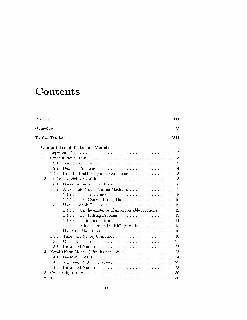
ContentsPreface IIIOverview VTo the Teacher VII1 Computational Tasks and Models 11.1 Representation : : : : : : : : : : : : : : : : : : : : : : : : : : : : : : 21.2 Computational Tasks : : : : : : : : : : : : : : : : : : : : : : : : : : : 31.2.1 Search Problems : : : : : : : : : : : : : : : : : : : : : : : : : 31.2.2 Decision Problems : : : : : : : : : : : : : : : : : : : : : : : : 41.2.3 Promise Problems (an advanced comment) : : : : : : : : : : 51.3 Uniform Models (Algorithms) : : : : : : : : : : : : : : : : : : : : : : 51.3.1 Overview and General Principles : : : : : : : : : : : : : : : : 51.3.2 A Concrete Model: Turing Machines : : : : : : : : : : : : : : 71.3.2.1 The actual model : : : : : : : : : : : : : : : : : : : 81.3.2.2 The Church-Turing Thesis : : : : : : : : : : : : : : 101.3.3 Uncomputable Functions : : : : : : : : : : : : : : : : : : : : 121.3.3.1 On the existence of uncomputable functions : : : : 121.3.3.2 The Halting Problem : : : : : : : : : : : : : : : : : 131.3.3.3 Turing-reductions : : : : : : : : : : : : : : : : : : : 141.3.3.4 A few more undecidability results : : : : : : : : : : 151.3.4 Universal Algorithms : : : : : : : : : : : : : : : : : : : : : : : 161.3.5 Time (and Space) Complexity : : : : : : : : : : : : : : : : : : 181.3.6 Oracle Machines : : : : : : : : : : : : : : : : : : : : : : : : : 211.3.7 Restricted Models : : : : : : : : : : : : : : : : : : : : : : : : 221.4 Non-Uniform Models (Circuits and Advice) : : : : : : : : : : : : : : 231.4.1 Boolean Circuits : : : : : : : : : : : : : : : : : : : : : : : : : 241.4.2 Machines That Take Advice : : : : : : : : : : : : : : : : : : : 271.4.3 Restricted Models : : : : : : : : : : : : : : : : : : : : : : : : 281.5 Complexity Classes : : : : : : : : : : : : : : : : : : : : : : : : : : : : 30Exercises : : : : : : : : : : : : : : : : : : : : : : : : : : : : : : : : : : : : 30IX

X CONTENTS2 The P versus NP Question 352.1 The Search Version: Finding Versus Checking : : : : : : : : : : : : : 362.1.1 The Class P as a Natural Class of Search Problems : : : : : : 372.1.2 The Class NP as Another Natural Class of Search Problems : 382.1.3 The P Versus NP Question in Terms of Search Problems : : : 392.2 The Decision Version: Proving Versus Verifying : : : : : : : : : : : : 402.2.1 The Class P as a Natural Class of Decision Problems : : : : : 412.2.2 The Class NP and NP-Proof Systems : : : : : : : : : : : : : 412.2.3 The P Versus NP Question in Terms of Decision Problems : : 442.3 Equivalence of the two Formulations : : : : : : : : : : : : : : : : : : 442.4 Technical Comments Regarding NP : : : : : : : : : : : : : : : : : : 452.5 The Traditional De�nition of NP : : : : : : : : : : : : : : : : : : : : 462.6 In Support of P Being Di�erent from NP : : : : : : : : : : : : : : : 482.7 Philosophical Meditations : : : : : : : : : : : : : : : : : : : : : : : : 49Exercises : : : : : : : : : : : : : : : : : : : : : : : : : : : : : : : : : : : : 503 Polynomial-time Reductions 533.1 The General Notion of a Reduction : : : : : : : : : : : : : : : : : : : 533.1.1 The Actual Formulation : : : : : : : : : : : : : : : : : : : : : 543.1.2 Special Cases : : : : : : : : : : : : : : : : : : : : : : : : : : : 553.1.3 Terminology and a Brief Discussion : : : : : : : : : : : : : : 563.2 Reducing Optimization Problems to Search Problems : : : : : : : : 563.3 Self-Reducibility of Search Problems : : : : : : : : : : : : : : : : : : 583.3.1 Examples : : : : : : : : : : : : : : : : : : : : : : : : : : : : : 603.3.2 Self-Reducibility of NP-Complete Problems : : : : : : : : : : 623.4 Digest and General Perspective : : : : : : : : : : : : : : : : : : : : : 62Exercises : : : : : : : : : : : : : : : : : : : : : : : : : : : : : : : : : : : : 634 NP-Completeness 674.1 De�nitions : : : : : : : : : : : : : : : : : : : : : : : : : : : : : : : : : 674.2 The Existence of NP-Complete Problems : : : : : : : : : : : : : : : 684.3 Some Natural NP-Complete Problems : : : : : : : : : : : : : : : : : 714.3.1 Circuit and Formula Satis�ability: CSAT and SAT : : : : : : 724.3.1.1 The NP-Completeness of CSAT : : : : : : : : : : : 724.3.1.2 The NP-Completeness of SAT : : : : : : : : : : : : 754.3.2 Combinatorics and Graph Theory : : : : : : : : : : : : : : : 784.4 NP sets that are Neither in P nor NP-Complete : : : : : : : : : : : : 844.5 Re ections on Complete Problems : : : : : : : : : : : : : : : : : : : 87Exercises : : : : : : : : : : : : : : : : : : : : : : : : : : : : : : : : : : : : 905 Three relatively advanced topics 975.1 Promise Problems : : : : : : : : : : : : : : : : : : : : : : : : : : : : 975.1.1 De�nitions : : : : : : : : : : : : : : : : : : : : : : : : : : : : 985.1.1.1 Search problems with a promise : : : : : : : : : : : 985.1.1.2 Decision problems with a promise : : : : : : : : : : 995.1.1.3 Reducibility among promise problems : : : : : : : : 100

CONTENTS XI5.1.2 Applications : : : : : : : : : : : : : : : : : : : : : : : : : : : 1005.1.3 The Standard Convention of Avoiding Promise Problems : : 1015.2 Optimal search algorithms for NP : : : : : : : : : : : : : : : : : : : 1035.3 The class coNP and its intersection with NP : : : : : : : : : : : : : : 105Exercises : : : : : : : : : : : : : : : : : : : : : : : : : : : : : : : : : : : : 108Notes 113Epilogue: A Brief Overview of Complexity Theory 117A Some Computational Problems 123A.1 Graphs : : : : : : : : : : : : : : : : : : : : : : : : : : : : : : : : : : : 123A.2 Boolean Formulae : : : : : : : : : : : : : : : : : : : : : : : : : : : : 126Bibliography 127

XII CONTENTS

List of Figures1.1 A single step by a Turing machine. : : : : : : : : : : : : : : : : : : : 91.2 A circuit computing f(x1; x2; x3; x4) = (x1 � x2; x1 ^ :x2 ^ x4). : : : 251.3 Recursive construction of parity circuits and formulae. : : : : : : : : 294.1 Consecutive computation steps of a Turing machine : : : : : : : : : 744.2 The idea underlying the reduction of CSAT to SAT : : : : : : : : : : 764.3 The reduction to G3C { the clause gadget and its sub-gadget : : : : 824.4 The reduction to G3C { connecting the gadgets : : : : : : : : : : : : 834.5 The (non-generic) reductions presented in Section 4.3 : : : : : : : : 845.1 The world view under P 6= coNP \NP 6= NP . : : : : : : : : : : : : 108

XIII

Chapter 1Computational Tasks andModelsThis chapter provides the necessary preliminaries for the rest of the book; that is,we discuss the notion of a computational task and present computational modelsfor describing methods for solving such tasks.We start by introducing the general framework for our discussion of computa-tional tasks (or problems). This framework refers to the representation of instancesas binary sequences (see Section 1.1) and focuses on two types of tasks: searchingfor solutions and making decisions (see Section 1.2).Once computational tasks are de�ned, we turn to methods for solving suchtasks, which are described in terms of some model of computation. The descriptionof such models is the main contents of this chapter. Speci�cally, we consider twotypes of models of computation: uniform models and non-uniform models (seeSections 1.3 and 1.4, respectively). The uniform models correspond to the intuitivenotion of an algorithm, and will provide the stage for the rest of the book (whichfocuses on e�cient algorithms). In contrast, non-uniform models (e.g., Booleancircuits) facilitate a closer look at the way a computation progresses, and will beonly used sporadically in this book.Additional comments about the contents of this chapter: Sections 1.1{1.3 corresponds to the contents of a traditional Computability course, except thatour presentation emphasizes some aspects and deemphasizes others. In particu-lar, the presentation highlights the notion of a universal machine (see Sec. 1.3.4),justi�es the association of e�cient computation with polynomial-time algorithm(Sec. 1.3.5), and provides a de�nition of oracle machines (Sec. 1.3.6). This mate-rial (with the exception of Kolmogorov Complexity) is taken for granted in the restof the current book. In contrast, Section 1.4 presents basic preliminaries regard-ing non-uniform models of computation (i.e., various types of Boolean circuits),and these are only used lightly in the rest of the book. (We also call the reader'sattention to the discussion of generic complexity classes in Section 1.5.) Thus,1

2 CHAPTER 1. COMPUTATIONAL TASKS AND MODELSwhereas Sections 1.1{1.3 (and 1.5) are absolute prerequisites for the rest of thisbook, Section 1.4 is not.Teaching note: The author believes that there is no real need for a semester-longcourse in Computability (i.e., a course that focuses on what can be computed ratherthan on what can be computed e�ciently). Instead, undergraduates should take acourse in Computational Complexity, which should contain the computability aspectsthat serve as a basis for the study of e�cient computation (i.e., the rest of this course).Speci�cally, the former aspects should occupy at most one third of the course, and thefocus should be on basic complexity issues (captured by P, NP, and NP-completeness),which may be augmented by a selection of some more advanced material. Indeed, sucha course can be based on the current book (possibly augmented by a selection of sometopics from, say, [13]).1.1 RepresentationIn mathematics and related sciences, it is customary to discuss objects withoutspecifying their representation. This is not possible in the theory of computation,where the representation of objects plays a central role. In a sense, a computationmerely transforms one representation of an object to another representation of thesame object. In particular, a computation designed to solve some problem merelytransforms the problem instance to its solution, where the latter can be thoughof as a (possibly partial) representation of the instance. Indeed, the answer toany fully speci�ed question is implicit in the question itself, and computation isemployed to make this answer explicit.Computational tasks refers to objects that are represented in some canonicalway, where such canonical representation provides an \explicit" and \full" (butnot \overly redundant") description of the corresponding object. We will consideronly �nite objects like numbers, sets, graphs, and functions (and keep distinguish-ing these types of objects although, actually, they are all equivalent). While therepresentation of numbers, sets and functions is quite straightforward, we refer thereader to Appendix A.1 for a discussion of the representation of graphs.In order to facilitate a study of methods for solving computational tasks, thelatter are de�ned with respect to in�nitely many possible instances (each being a�nite object). Indeed, the comparison of di�erent methods seems to require theconsideration of in�nitely many possible instances; otherwise, the choice of the lan-guage in which the methods are described may totally dominated and even distortthe discussion (cf., e.g., the discussion of Kolmogorov Complexity in Sec. 1.3.4).Strings. We consider �nite objects, each represented by a �nite binary sequence,called a string. For a natural number n, we denote by f0; 1gn the set of all stringsof length n, hereafter referred to as n-bit (long) strings. The set of all strings isdenoted f0; 1g�; that is, f0; 1g� = [n2Nf0; 1gn. For x2 f0; 1g�, we denote by jxjthe length of x (i.e., x 2 f0; 1gjxj), and often denote by xi the ith bit of x (i.e.,

1.2. COMPUTATIONAL TASKS 3x = x1x2 � � �xjxj). For x; y 2 f0; 1g�, we denote by xy the string resulting fromconcatenation of the strings x and y.At times, we associate f0; 1g��f0; 1g� with f0; 1g�; the reader should merelyconsider an adequate encoding (e.g., the pair (x1 � � �xm; y1 � � � yn)2f0; 1g��f0; 1g�may be encoded by the string x1x1 � � �xmxm01y1 � � � yn 2 f0; 1g�). Likewise, wemay represent sequences of strings (of �xed or varying length) as single strings.When we wish to emphasize that such a sequence (or some other object) is to beconsidered as a single object we use the notation h�i (e.g., \the pair (x; y) is encodedas the string hx; yi").Numbers. Unless stated di�erently, natural numbers will be encoded by theirbinary expansion; that is, the string bn�1 � � � b1b0 2 f0; 1gn encodes the numberPn�1i=0 bi � 2i, where typically we assume that this representation has no leadingzeros (i.e., bn�1 = 1). Rational numbers will be represented as pairs of naturalnumbers. In the rare cases in which one considers real numbers as part of theinput to a computational problem, one actually mean rational approximations ofthese real numbers.Special symbols. We denote the empty string by � (i.e., � 2 f0; 1g� and j�j = 0),and the empty set by ;. It will be convenient to use some special symbols that arenot in f0; 1g�. One such symbol is ?, which typically denotes an indication (e.g.,produced by some algorithm) that something is wrong.1.2 Computational TasksTwo fundamental types of computational tasks are the so-called search problemsand decision problems. In both cases, the key notions are the problem's instancesand the problem's speci�cation.1.2.1 Search ProblemsA search problem consists of a speci�cation of a set of valid solutions (possibly anempty one) for each possible instance. That is, given an instance, one is requiredto �nd a corresponding solution (or to determine that no such solution exists).For example, consider the problem in which one is given a system of equationsand is asked to �nd a valid solution. Needless to say, much of computer scienceis concerned with solving various search problems (e.g., �nding shortest paths ina graph, sorting a list of numbers, �nding an occurrence of a given pattern in agiven string, etc). Furthermore, search problems correspond to the daily notionof \solving a problem" (e.g., �nding one's way between two locations), and thus adiscussion of the possibility and complexity of solving search problems correspondsto the natural concerns of most people.In the following de�nition of solving search problems, the potential solver is afunction (which may be thought of as a solving strategy), and the sets of possible

4 CHAPTER 1. COMPUTATIONAL TASKS AND MODELSsolutions associated with each of the various instances are \packed" into a singlebinary relation.De�nition 1.1 (solving a search problem): Let R � f0; 1g��f0; 1g� and R(x) def=fy : (x; y) 2 Rg denote the set of solutions for the instance x. A function f :f0; 1g� ! f0; 1g� [ f?g solves the search problem of R if for every x the followingholds: if R(x) 6= ; then f(x) 2 R(x) and otherwise f(x) = ?.Indeed, R = f(x; y)2f0; 1g� � f0; 1g� : y2R(x)g, and the solver f is required to�nd a solution (i.e., given x output y 2 R(x)) whenever one exists (i.e., the setR(x) is not empty). It is also required that the solver f never outputs a wrongsolution (i.e., if R(x) 6= ; then f(x) 2 R(x) and if R(x) = ; then f(x) = ?), whichin turn means that f indicates whether x has any solution.A special case of interest is the case of search problems having a unique solution(for each possible instance); that is, the case that jR(x)j = 1 for every x. In thiscase, R is essentially a (total) function, and solving the search problem of R meanscomputing (or evaluating) the function R (or rather the function R0 de�ned byR0(x) def= y if and only if R(x) = fyg). Popular examples include sorting a sequenceof numbers, multiplying integers, �nding the prime factorization of a compositenumber, etc.1.2.2 Decision ProblemsA decision problem consists of a speci�cation of a subset of the possible instances.Given an instance, one is required to determine whether the instance is in thespeci�ed set (e.g., the set of prime numbers, the set of connected graphs, or theset of sorted sequences). For example, consider the problem where one is given anatural number, and is asked to determine whether or not the number is a prime.One important case, which corresponds to the aforementioned search problems, isthe case of the set of instances having a solution (w.r.t some �xed search problem);that is, for any binary relation R � f0; 1g��f0; 1g� we consider the set fx : R(x) 6=;g. Indeed, being able to determine whether or not a solution exists is a prerequisiteto being able to solve the corresponding search problem (as per De�nition 1.1).In general, decision problems refer to the natural task of making binary decision,a task that is not uncommon in daily life (e.g., determining whether a tra�c lightis red). In any case, in the following de�nition of solving decision problems, thepotential solver is again a function; that is, in this case the solver is a Booleanfunction, which is supposed to indicate membership in a predetermined set.De�nition 1.2 (solving a decision problem): Let S � f0; 1g�. A function f :f0; 1g� ! f0; 1g solves the decision problem of S (or decides membership in S) if forevery x it holds that f(x) = 1 if and only if x 2 S.We often identify the decision problem of S with S itself, and identify S with itscharacteristic function (i.e., with the function �S : f0; 1g� ! f0; 1g de�ned suchthat �S(x) = 1 if and only if x 2 S). Note that if f solves the search problem of R

1.3. UNIFORM MODELS (ALGORITHMS) 5then the Boolean function f 0 : f0; 1g� ! f0; 1g de�ned by f 0(x) def= 1 if and only iff(x) 6= ? solves the decision problem of fx : R(x) 6= ;g.Re ection: Most people would consider search problems to be more natural thandecision problems: typically, people seeks solutions more often than they stop towonder whether or not solutions exist. De�nitely, search problems are not lessimportant than decision problems, it is merely that their study tends to requiremore cumbersome formulations. This is the main reason that most expositionschoose to focus on decision problems. The current book attempts to devote atleast a signi�cant amount of attention also to search problems.1.2.3 Promise Problems (an advanced comment)Many natural search and decision problems are captured more naturally by theterminology of promise problems, in which the domain of possible instances is asubset of f0; 1g� rather than f0; 1g� itself. In particular, note that the naturalformulation of many search and decision problems refers to instances of a certaintype (e.g., a system of equations, a pair of numbers, a graph), whereas the naturalrepresentation of these objects uses only a strict subset of f0; 1g�. For the timebeing, we ignore this issue, but we shall re-visit it in Section 5.1. Here we justnote that, in typical cases, the issue can be ignored by postulating that everystring represents some legitimate object (e.g., each string that is not used in thenatural representation of these objects is postulated as a representation of some�xed object).1.3 Uniform Models (Algorithms)We �nally reach the heart of the current chapter, which is the de�nition of (uniform)models of computation. Before presenting such models, let us brie y motivate theneed for their formal de�nitions. Indeed, we are all familiar with computers andwith the ability of computer programs to manipulate data. But this familiarityis rooted in positive experience; that is, we have some experience regarding somethings that computers can do. In contrast, complexity theory is focused at whatcomputers cannot do, or rather with drawing the line between what can be doneand what cannot be done. Drawing such a line requires a precise formulation ofall possible computational processes; that is, we should have a clear de�nitionof all possible computational processes (rather than some familiarity with somecomputational processes).1.3.1 Overview and General PrinciplesBefore being formal, let we o�er a general and abstract description of the notionof computation. This description applies both to arti�cial processes (taking placein computers) and to processes that are aimed at modeling the evolution of thenatural reality (be it physical, biological, or even social).

6 CHAPTER 1. COMPUTATIONAL TASKS AND MODELSA computation is a process that modi�es an environment via repeated applica-tions of a predetermined rule. The key restriction is that this rule is simple: in eachapplication it depends and a�ects only a (small) portion of the environment, calledthe active zone. We contrast the a-priori bounded size of the active zone (and ofthe modi�cation rule) with the a-priori unbounded size of the entire environment.We note that, although each application of the rule has a very limited e�ect, thee�ect of many applications of the rule may be very complex. Put in other words, acomputation may modify the relevant environment in a very complex way, althoughit is merely a process of repeatedly applying a simple rule.As hinted, the notion of computation can be used to model the \mechanical"aspects of the natural reality; that is, the rules that determine the evolution ofthe reality (rather than the speci�c state of the reality at a speci�c time). In thiscase, the starting point of the study is the actual evolution process that takes placein the natural reality, and the goal of the study is �nding the (computation) rulethat underlies this natural process. In a sense, the goal of science at large can bephrased as �nding (simple) rules that govern various aspects of reality (or ratherone's abstraction of these aspects of reality).Our focus, however, is on arti�cial computation rules designed by humans inorder to achieve speci�c desired e�ects on a corresponding arti�cial environment.Thus, our starting point is a desired functionality, and our aim is to design compu-tation rules that e�ect it. Such a computation rule is referred to as an algorithm.Loosely speaking, an algorithm corresponds to a computer program written in ahigh-level (abstract) programming language. Let us elaborate.We are interested in the transformation of the environment as e�ected by thecomputational process (or the algorithm). Throughout (almost all of) this book, wewill assume that, when invoked on any �nite initial environment, the computationhalts after a �nite number of steps. Typically, the initial environment to whichthe computation is applied encodes an input string, and the end environment (i.e.,at termination of the computation) encodes an output string. We consider themapping from inputs to outputs induced by the computation; that is, for eachpossible input x, we consider the output y obtained at the end of a computationinitiated with input x, and say that the computation maps input x to output y.Thus, a computation rule (or an algorithm) determines a function (computed byit): this function is exactly the aforementioned mapping of inputs to outputs.In the rest of this book (i.e., outside the current chapter), we will also considerthe number of steps (i.e., applications of the rule) taken by the computation oneach possible input. The latter function is called the time complexity of the com-putational process (or algorithm). While time complexity is de�ned per input, wewill often considers it per input length, taking the maximum over all inputs of thesame length.In order to de�ne computation (and computation time) rigorously, one needsto specify some model of computation; that is, provide a concrete de�nition ofenvironments and a class of rules that may be applied to them. Such a model cor-responds to an abstraction of a real computer (be it a PC, mainframe or networkof computers). One simple abstract model that is commonly used is that of Tur-

1.3. UNIFORM MODELS (ALGORITHMS) 7ing machines (see, Sec. 1.3.2). Thus, speci�c algorithms are typically formalizedby corresponding Turing machines (and their time complexity is represented bythe time complexity of the corresponding Turing machines). We stress, however,that almost all results in the Theory of Computation hold regardless of the speci�ccomputational model used, as long as it is \reasonable" (i.e., satis�es the aforemen-tioned simplicity condition and can perform some apparently simple computations).What is being computed? The foregoing discussion has implicitly referredto algorithms (i.e., computational processes) as means of computing functions.Speci�cally, an algorithm A computes the function fA :f0; 1g�!f0; 1g� de�ned byfA(x)=y if, when invoked on input x, algorithm A halts with output y. However,algorithms can also serve as means of \solving search problems" or \making de-cisions" (as in De�nitions 1.1 and 1.2). Speci�cally, we will say that algorithm Asolves the search problem of R (resp., decides membership in S) if fA solves thesearch problem of R (resp., decides membership in S). In the rest of this expositionwe associate the algorithm A with the function fA computed by it; that is, we writeA(x) instead of fA(x). For sake of future reference, we summarize the foregoingdiscussion in a de�nition.De�nition 1.3 (algorithms as problem-solvers): We denote by A(x) the outputof algorithm A on input x. Algorithm A solves the search problem R (resp., thedecision problem S) if A, viewed as a function, solves R (resp., S).Organization of the rest of Section 1.3. In Sec. 1.3.2 we provide a roughdescription of the model of Turing machines. This is done merely for sake of pro-viding a concrete model that supports the study of computation and its complexity,whereas the material in this book will not depend on the speci�cs of this model. InSec. 1.3.3 and Sec. 1.3.4 we discuss two fundamental properties of any reasonablemodel of computation: the existence of uncomputable functions and the existenceof universal computations. The time (and space) complexity of computation isde�ned in Sec. 1.3.5. We also discuss oracle machines and restricted models ofcomputation (in Sec. 1.3.6 and Sec. 1.3.7, respectively).1.3.2 A Concrete Model: Turing MachinesThe model of Turing machines o�er a relatively simple formulation of the notionof an algorithm. The fact that the model is very simple complicates the design ofmachines that solve problems of interest, but makes the analysis of such machinessimpler. Since the focus of complexity theory is on the analysis of machines and noton their design, the trade-o� o�ers by this model is suitable for our purposes. Westress again that the model is merely used as a concrete formulation of the intuitivenotion of an algorithm, whereas we actually care about the intuitive notion andnot about its formulation. In particular, all results mentioned in this book hold forany other \reasonable" formulation of the notion of an algorithm.

8 CHAPTER 1. COMPUTATIONAL TASKS AND MODELSThe model of Turing machines is not meant to provide an accurate (or \tight")model of real-life computers, but rather to capture their inherent limitations andabilities (i.e., a computational task can be solved by a real-life computer if and onlyif it can be solved by a Turing machine). In comparison to real-life computers, themodel of Turing machines is extremely over-simpli�ed and abstract away manyissues that are of great concern to computer practice. However, these issues areirrelevant to the higher-level questions addressed by complexity theory. Indeed, asusual, good practice requires more re�ned understanding than the one provided bya good theory, but one should �rst provide the latter.Historically, the model of Turing machines was invented before modern com-puters were even built, and was meant to provide a concrete model of computationand a de�nition of computable functions.1 Indeed, this concrete model clari�edfundamental properties of computable functions and plays a key role in de�ningthe complexity of computable functions.The model of Turing machines was envisioned as an abstraction of the processof an algebraic computation carried out by a human using a sheet of paper. Insuch a process, at each time, the human looks at some location on the paper, anddepending on what he/she sees and what he/she has in mind (which is little...),he/she modi�es the contents of this location and shifts his/her look to an adjacentlocation.1.3.2.1 The actual modelFollowing is a high-level description of the model of Turing machines; the interestedreader is referred to standard textbooks (e.g., [29]) for further details. Recallthat we need to specify the set of possible environments, the set of machines (orcomputation rules), and the e�ect of applying such a rule on an environment.The environment. The main component in the environment of a Turing ma-chine is an in�nite sequence of cells, each capable of holding a single symbol (i.e.,member of a �nite set � � f0; 1g). This sequence is envisioned as starting at aleft-most cell, and extending in�nitely to the right (cf., Figure 1.1). In addition,the environment contains the current location of the machine on this sequence, andthe internal state of the machine (which is a member of a �nite set Q). The afore-mentioned sequence of cells is called the tape, and its contents combined with themachine's location and its internal state is called the instantaneous con�guration ofthe machine.The machine itself (i.e., the computation rule). The main component inthe Turing machine itself is a �nite rule (i.e., a �nite function), called the transitionfunction, which is de�ned over the set of all possible symbol-state pairs. Speci�cally,the transition function is a mapping from � � Q to � � Q � f�1; 0;+1g, where1In contrast, the abstract de�nition of \recursive functions" yields a class of \computable"functions without referring to any model of computation (but rather based on the intuition thatany such model should support recursive functional composition).

1.3. UNIFORM MODELS (ALGORITHMS) 93 32 2 2 0

3 32 2 2 1 0

b

3

b

5

5

- - - - - - - -

----- - - -Figure 1.1: A single step by a Turing machine.f�1;+1; 0g correspond to a movement instruction (which is either \left" or \right"or \stay", respectively). In addition, the machine's description speci�es an initialstate and a halting state, and the computation of the machine halts when themachine enters its halting state. (Envisioning the tape as in Figure 1.1, we use theconvention by which if the machine tries to move left of the end of the tape thenit is considered to have halted.)We stress that, in contrast to the �nite description of the machine, the tape hasan a priori unbounded length (and is considered, for simplicity, as being in�nite).A single application of the computation rule. A single computation step ofsuch a Turing machine depends on its current location on the tape, on the contentsof the corresponding cell, and on the internal state of the machine. Based on thelatter two elements, the transition function determines a new symbol-state pair aswell as a movement instruction (i.e., \left" or \right" or \stay"). The machinemodi�es the contents of the said cell and its internal state accordingly, and movesas directed. That is, suppose that the machine is in state q and resides in a cellcontaining the symbol �, and suppose that the transition function maps (�; q) to(�0; q0; D). Then, the machine modi�es the contents of the said cell to �0, modi�esits internal state to q0, and moves one cell in direction D. Figure 1.1 shows asingle step of a Turing machine that, when in state `b' and seeing a binary symbol�, replaces � with the symbol � + 2, maintains its internal state, and moves oneposition to the right.2Formally, we de�ne the successive con�guration function which maps each in-stantaneous con�guration to the one resulting by letting the machine take a singlestep. This function modi�es its argument in a very minor manner, as describedin the foregoing paragraph; that is, the contents of at most one cell (i.e., at whichthe machine currently resides) is changed, and in addition the internal state of themachine and its location may change too.2Figure 1.1 corresponds to a machine that, when in the initial state (i.e., `a'), replaces thesymbol � by �+4, modi�es its internal state to `b', and moves one position to the right. Indeed,\marking" the leftmost cell (in order to allow for recognizing it in the future), is a commonpractice in the design of Turing machines.

10 CHAPTER 1. COMPUTATIONAL TASKS AND MODELSInitial and �nal environments. The initial environment (or con�guration) ofa Turing machine consists of the machine residing in the �rst (i.e., left-most) celland being in its initial state. Typically, one also mandates that, in the initial con-�guration, a pre�x of the tape's cells hold bit values, which concatenated togetherare considered the input, and the rest of the tape's cells hold a special symbol(which in Figure 1.1 is denoted by `-'). Once the machine halts, the output is de-�ned as the contents of the cells that are to the left of its location (at terminationtime).3 Thus, each machine de�nes a function mapping inputs to outputs, calledthe function computed by the machine.Multi-tape Turing machines. We comment that in most expositions, onerefers to the location of the \head of the machine" on the tape (rather than tothe \location of the machine on the tape"). The standard terminology is moreintuitive when extending the basic model, which refers to a single tape, to a modelthat supports a constant number of tapes. In the corresponding model of so-calledmulti-tape machines, the machine maintains a single head on each such tape, andeach step of the machine depends and e�ects the cells that are at the machine'shead location on each tape. (The input is given on one designated tape, and theoutput is required to appear on some other designated tape.) As we shall see inSection 1.3.5, the extension of the model to multi-tape Turing machines is crucialto the de�nition of space complexity. A less fundamental advantage of the modelof multi-tape Turing machines is that it facilitates the design of machines thatcompute functions of interest.Teaching note: We strongly recommend avoiding the standard practice of teachingthe student to program with Turing machines. These exercises seem very painful andpointless. Instead, one should prove that the Turing machine model is exactly as pow-erful as a model that is closer to a real-life computer (see the following \sanity check");that is, a function can be computed by a Turing machine if and only if it is computableby a machine of the latter model. For starters, one may prove that a function can becomputed by a single-tape Turing machine if and only if it is computable by a multi-tape(e.g., two-tape) Turing machine.1.3.2.2 The Church-Turing ThesisThe entire point of the model of Turing machines is its simplicity. That is, incomparison to more \realistic" models of computation, it is simpler to formu-late the model of Turing machines and to analyze machines in this model. TheChurch-Turing Thesis asserts that nothing is lost by considering the Turing ma-chine model: A function can be computed by some Turing machine if and only ifit can be computed by some machine of any other \reasonable and general" modelof computation.3By an alternative convention, the machine halts while residing in the left-most cell, and theoutput is de�ned as the maximal pre�x of the tape contents that contains only bit values.

1.3. UNIFORM MODELS (ALGORITHMS) 11This is a thesis, rather than a theorem, because it refers to an intuitive notion(i.e., the notion of a reasonable and general model of computation) that is left unde-�ned on purpose. The model should be reasonable in the sense that it should allowonly computation rules that are \simple" in some intuitive sense. For example,we should be able to envision a mechanical implementation of these computationrules. On the other hand, the model should allow to compute \simple" functionsthat are de�nitely computable according to our intuition. At the very least themodel should allow to emulate Turing machines (i.e., compute the function that,given a description of a Turing machine and an instantaneous con�guration, returnsthe successive con�guration).A philosophical comment. The fact that a thesis is used to link an intuitiveconcept to a formal de�nition is common practice in any science (or, more broadly,in any attempt to reason rigorously about intuitive concepts). Any attempt torigorously de�ne an intuitive concept yields a formal de�nition that necessarilydi�ers from the original intuition, and the question of correspondence between thesetwo objects arises. This question can never be rigorously treated, because one ofthe objects that it relates to is unde�ned. That is, the question of correspondencebetween the intuition and the de�nition always transcends a rigorous treatment(i.e., it always belongs to the domain of the intuition).A sanity check: Turing machines can emulate an abstract RAM. To gaincon�dence in the Church-Turing Thesis, one may attempt to de�ne an abstractRandom-Access Machine (RAM), and verify that it can be emulated by a Turingmachine. An abstract RAM consists of an in�nite number of memory cells, eachcapable of holding an integer, a �nite number of similar registers, one designatedas program counter, and a program consisting of instructions selected from a �niteset. The set of possible instructions includes the following instructions:� reset(r), where r is an index of a register, results in setting the value ofregister r to zero.� inc(r), where r is an index of a register, results in incrementing the contentof register r. Similarly dec(r) causes a decrement.� load(r1; r2), where r1 and r2 are indices of registers, results in loading toregister r1 the contents of the memory location m, where m is the currentcontents of register r2.� store(r1; r2), stores the contents of register r1 in the memory, analogouslyto load.� cond-goto(r; `), where r is an index of a register and ` does not exceed theprogram length, results in setting the program counter to `� 1 if the contentof register r is non-negative.The program counter is incremented after the execution of each instruction, andthe next instruction to be executed by the machine is the one to which the programcounter points (and the machine halts if the program counter exceeds the program's

12 CHAPTER 1. COMPUTATIONAL TASKS AND MODELSlength). The input to the machine may be de�ned as the contents of the �rst nmemory cells, where n is placed in a special input register.We note that the abstract RAM model (as de�ned above) is as powerful asthe Turing machine model (see the following details). However, in order to makethe RAM model closer to real-life computers, we may augment it with additionalinstructions that are available on real-life computers like the instruction add(r1; r2)(resp., mult(r1; r2)) that results in adding (resp., multiplying) the contents of reg-isters r1 and r2 (and placing the result in register r1). We suggest proving thatthis abstract RAM can be emulated by a Turing machine: see Exercise 1.4. Weemphasize this direction of the equivalence of the two models, because the RAMmodel is introduced in order to convince the reader that Turing machines are nottoo weak (as a model of general computation). The fact that they are not toostrong seems self-evident. Thus, it seems pointless to prove that the RAM modelcan emulate Turing machines. (Still, note that this is indeed the case, by usingthe RAM's memory cells to store the contents of the cells of the Turing machine'stape, and holding its head location in a special register.)Re ections: Observe that the abstract RAM model is signi�cantly more cum-bersome than the Turing machine model. Furthermore, seeking a sound choiceof the instruction set (i.e., the instructions to be allowed in the model) createsa vicious cycle (because the sound guideline for such a choice should have beenallowing only instructions that correspond to \simple" operations, whereas the lat-ter correspond to easily computable functions...). This vicious cycle was avoided inthe foregoing paragraph by trusting the reader to include only instructions that areavailable in some real-life computer. (We comment that this empirical considera-tion is justi�able in the current context, because our current goal is merely linkingthe Turing machine model with the reader's experience of real-life computers.)1.3.3 Uncomputable FunctionsStrictly speaking, the current subsection is not necessary for the rest of this book,but we feel that it provides a useful perspective.1.3.3.1 On the existence of uncomputable functionsIn contrast to what every layman would think, we know that not all functions arecomputable. Indeed, an important message to be communicated to the world isthat not every well-de�ned task can be solved by applying a \reasonable" automatedprocedure (i.e., a procedure that has a simple description that can be applied toany instance of the problem at hand). Furthermore, not only is it the case thatthere exist uncomputable functions, but it is rather the case that most functionsare uncomputable. In fact, only relatively few functions are computable.Theorem 1.4 (on the scarcity of computable functions): The set of computablefunctions is countable, whereas the set of all functions (from strings to string) hascardinality @.

1.3. UNIFORM MODELS (ALGORITHMS) 13We stress that the theorem holds for any reasonable model of computation. Infact, it only relies on the postulate that each machine in the model has a �nitedescription (i.e., can be described by a string).Proof: Since each computable function is computable by a machine that hasa �nite description, there is a 1-1 mapping of computable functions to strings(whereas the set of all strings is in 1-1 correspondence to the natural numbers). Onthe other hand, there is a 1-1 correspondence between the set of Boolean functions(i.e., functions from strings to a single bit) and the set of real number in [0; 1).This correspondence associates each real r 2 [0; 1) to the function f : N ! f0; 1gsuch that f(i) is the ith bit in the in�nite binary expansion of r.1.3.3.2 The Halting ProblemIn contrast to the discussion in Sec. 1.3.1, at this point we consider also machinesthat may not halt on some inputs. The functions computed by such machines arepartial functions that are de�ned only on inputs on which the machine halts. Again,we rely on the postulate that each machine in the model has a �nite description,and denote the description of machine M by hMi 2 f0; 1g�. The halting function,h : f0; 1g� � f0; 1g� ! f0; 1g, is de�ned such that h(hMi; x) def= 1 if and only if Mhalts on input x. The following result goes beyond Theorem 1.4 by pointing to anexplicit function (of natural interest) that is not computable.Theorem 1.5 (undecidability of the halting problem): The halting function is notcomputable.The term undecidability means that the corresponding decision problem cannot besolved by an algorithm. That is, Theorem 1.5 asserts that the decision problemassociated with the set h�1(1) = f(hMi; x) : h(hMi; x) = 1g is not solvable byan algorithm (i.e., there exists no algorithm that, given a pair (hMi; x), decideswhether or notM halts on input x). Actually, the following proof shows that thereexists no algorithm that, given hMi, decides whether or notM halts on input hMi.Proof: We will show that even the restriction of h to its \diagonal" (i.e., the func-tion d(hMi) def= h(hMi; hMi)) is not computable. Note that the value of d(hMi)refers to the question of what happens when we feed M with its own description,which is indeed a \nasty" (but legitimate) thing to do. We will actually do some-thing \worse": towards the contradiction, we will consider the value of d whenevaluated at a (machine that is related to a) hypothetical machine that supposedlycomputes d.We start by considering a related function, d0, and showing that this functionis uncomputable. The function d0 is de�ned on purpose so to foil any attempt tocompute it; that is, for every machine M , the value d0(hMi) is de�ned to di�erfrom M(hMi). Speci�cally, the function d0 : f0; 1g� ! f0; 1g is de�ned suchthat d0(hMi) def= 1 if and only if M halts on input hMi with output 0. That is,d0(hMi) = 0 if either M does not halt on input hMi or its output does not equal

14 CHAPTER 1. COMPUTATIONAL TASKS AND MODELSthe value 0. Now, suppose, towards the contradiction, that d0 is computable bysome machine, denoted Md0 . Note that machine Md0 is supposed to halt on everyinput, and so Md0 halts on input hMd0i. But, by de�nition of d0, it holds thatd0(hMd0i) = 1 if and only if Md0 halts on input hMd0i with output 0 (i.e., if andonly if Md0(hMd0i) = 0). Thus, Md0(hMd0i) 6= d0(hMd0i) in contradiction to thehypothesis that Md0 computes d0.We next prove that d is uncomputable, and thus h is uncomputable (becaused(z) = h(z; z) for every z). To prove that d is uncomputable, we show that if dis computable then so is d0 (which we already know not to be the case). Indeed,suppose towards the contradiction that A is an algorithm for computing d (i.e.,A(hMi) = d(hMi) for every machine M). Then we construct an algorithm forcomputing d0, which given hM 0i, invokes A on hM 00i, where M 00 is de�ned tooperate as follows:1. On input x, machine M 00 emulates M 0 on input x.2. If M 0 halts on input x with output 0 then M 00 halts.3. If M 0 halts on input x with an output di�erent from 0 then M 00 enters anin�nite loop (and thus does not halt).Otherwise (i.e., M 0 does not halt on input x), then machine M 00 does nothalt (because it just stays stuck in Step 1 forever).Note that the mapping from hM 0i to hM 00i is easily computable (by augmentingM 0 with instructions to test its output and enter an in�nite loop if necessary), andthat d(hM 00i) = d0(hM 0i), becauseM 00 halts on x if and only if M 00 halts on x withoutput 0. We thus derived an algorithm for computing d0 (i.e., transform the inputhM 0i into hM 00i and output A(hM 00i)), which contradicts the already establishedfact by which d0 is uncomputable.1.3.3.3 Turing-reductionsThe core of the second part of the proof of Theorem 1.5 is an algorithm thatsolves one problem (i.e., computes d0) by using as a subroutine an algorithm thatsolves another problem (i.e., computes d (or h)). In fact, the �rst algorithm isactually an algorithmic scheme that refers to a \functionally speci�ed" subroutinerather than to an actual (implementation of such a) subroutine, which may notexist. Such an algorithmic scheme is called a Turing-reduction (see formulation inSec. 1.3.6). Hence, we have Turing-reduced the computation of d0 to the computa-tion of d, which in turn Turing-reduces to h. The \natural" (\positive") meaning ofa Turing-reduction of f 0 to f is that, when given an algorithm for computing f , weobtain an algorithm for computing f 0. In contrast, the proof of Theorem 1.5 usesthe \unnatural" (\negative") counter-positive: if (as we know) there exists no al-gorithm for computing f 0 = d0 then there exists no algorithm for computing f = d(which is what we wanted to prove). Jumping ahead, we mention that resource-bounded Turing-reductions (e.g., polynomial-time reductions) play a central rolein complexity theory itself, and again they are used mostly in a \negative" way.We will de�ne such reductions and extensively use them in subsequent chapters.

1.3. UNIFORM MODELS (ALGORITHMS) 151.3.3.4 A few more undecidability resultsWe brie y review a few appealing results regarding undecidable problems.Rice's Theorem. The undecidability of the halting problem (or rather the factthat the function d is uncomputable) is a special case of a more general phe-nomenon: Every non-trivial decision problem regarding the function computed bya given Turing machine has no algorithmic solution. We state this fact next, clar-ifying the de�nition of the aforementioned class of problems. (Again, we refer toTuring machines that may not halt on all inputs.)Theorem 1.6 (Rice's Theorem): Let F be any non-trivial subset4 of the set of allcomputable partial functions, and let SF be the set of strings that describe machinesthat compute functions in F . Then deciding membership in SF cannot be solved byan algorithm.Theorem 1.6 can be proved by a Turing-reduction from d. We do not provide a proofbecause this is too remote from the main subject matter of the book. (Still, theinterested reader is referred to Exercise 1.5.) We stress that Theorems 1.5 and 1.6hold for any reasonable model of computation (referring both to the potentialsolvers and to the machines the description of which is given as input to thesesolvers). Thus, Theorem 1.6 means that no algorithm can determine any non-trivial property of the function computed by a given computer program (written inany programming language). For example, no algorithm can determine whether ornot a given computer program halts on each possible input. The relevance of thisassertion to the project of program veri�cation is obvious.The Post Correspondence Problem. We mention that undecidability arisesalso outside of the domain of questions regarding computing devices (given asinput). Speci�cally, we consider the Post Correspondence Problem in which the inputconsists of two sequences of (non-empty) strings, (�1; :::; �k) and (�1; :::; �k), andthe question is whether or not there exists a sequence of indices i1; :::; i` 2 f1; :::; kgsuch that �i1 � � ��i` = �i1 � � ��i` . (We stress that the length of this sequence is nota priori bounded.)5Theorem 1.7 The Post Correspondence Problem is undecidable.Again, the omitted proof is by a Turing-reduction from d (or h), and the interestedreader is referred to Exercise 1.6.4The set S is called a non-trivial subset of U if both S and U n S are non-empty. Clearly, if Fis a trivial set of computable functions then the corresponding decision problem can be solved bya \trivial" algorithm that outputs the corresponding constant bit.5In contrast, the existence of an adequate sequence of a speci�ed length can be determined intime that is exponential in this length.

16 CHAPTER 1. COMPUTATIONAL TASKS AND MODELS1.3.4 Universal AlgorithmsSo far we have used the postulate that, in any reasonable model of computation,each machine (or computation rule) has a �nite description. Furthermore, wealso used the fact that such model should allow for the easy modi�cation of suchdescriptions such that the resulting machine computes an easily related function(see the proof of Theorem 1.5). Here we go one step further and postulate that thedescription of machines (in this model) is \e�ective" in the following natural sense:there exists an algorithm that, given a description of a machine (resp., computationrule) and a corresponding environment, determines the environment that resultsfrom performing a single step of this machine on this environment (resp. the e�ectof a single application of the computation rule). This algorithm can, in turn, beimplemented in the said model of computation (assuming this model is general; seethe Church-Turing Thesis). Successive applications of this algorithm leads to thenotion of a universal machine, which (for concreteness) is formulated next in termsof Turing machines.De�nition 1.8 (universal machines): A universal Turing machine is a Turing ma-chine that on input a description of a machine M and an input x returns the valueof M(x) if M halts on x and otherwise does not halt.That is, a universal Turing machine computes the partial function u on pairs(hMi; x) such that M halts on input x, in which case it holds that u(hMi; x) =M(x). That is, u(hMi; x) = M(x) if M halts on input x, and u is unde�ned on(hMi; x) otherwise. We note that if M halts on all possible inputs then u(hMi; x)is de�ned for every x.We stress that the mere fact that we have de�ned something (i.e., a universalTuring machine) does not mean that it exists. Yet, as hinted in the foregoing dis-cussion and obvious to anyone who has written a computer program (and thoughtabout what he/she was doing), universal Turing machines do exist.Theorem 1.9 There exists a universal Turing machine.Theorem 1.9 asserts that the partial function u is computable. In contrast, it canbe shown that any extension of u to a total function is uncomputable. That is, forany total function u that agrees with the partial function u on all the inputs onwhich the latter is de�ned, it holds that u is uncomputable (see Exercise 1.7).Proof: Given a pair (hMi; x), we just emulate the computation of machine Mon input x. This emulation is straightforward, because (by the e�ectiveness of thedescription ofM) we can iteratively determine the next instantaneous con�gurationof the computation of M on input x. If the said computation halts then we willobtain its output and can output it (and so, on input (hMi; x), our algorithmreturns M(x)). Otherwise, we turn out emulating an in�nite computation, whichmeans that our algorithm does not halt on input (hMi; x). Thus, the foregoingemulation procedure constitutes a universal machine (i.e., yields an algorithm forcomputing u).

1.3. UNIFORM MODELS (ALGORITHMS) 17As hinted already, the existence of universal machines is the fundamental factunderlying the paradigm of general-purpose computers. Indeed, a speci�c Turingmachine (or algorithm) is a device that solves a speci�c problem. A priori, solvingeach problem would have required building a new physical device that allows forthis problem to be solved in the physical world (rather than as a thought experi-ment). The existence of a universal machine asserts that it is enough to build onephysical device; that is, a general purpose computer. Any speci�c problem canthen be solved by writing a corresponding program to be executed (or emulated)by the general-purpose computer. Thus, universal machines correspond to general-purpose computers, and provide the basis for separating hardware from software.Furthermore, the existence of universal machines says that software can be viewedas (part of the) input.In addition to their practical importance, the existence of universal machines(and their variants) has important consequences in the theories of computabilityand computational complexity. To demonstrate the point, we note that Theo-rem 1.6 implies that many questions about the behavior of a �xed universal ma-chine on certain input types are undecidable. For example, it follows that, forsome �xed machines (i.e., universal ones), there is no algorithm that determineswhether or not the (�xed) machine halts on a given input. Revisiting the proof ofTheorem 1.7 (see Exercise 1.6), it follows that the Post Correspondence Problemremains undecidable even if the input sequences are restricted to have a speci�clength (i.e., k is �xed). A more important application of universal machines to thetheory of computability follows.A detour: Kolmogorov Complexity. The existence of universal machines,which may be viewed as universal languages for writing e�ective and succinctdescriptions of objects, plays a central role in Kolmogorov Complexity. Looselyspeaking, the latter theory is concerned with the length of (e�ective) descriptionsof objects, and views the minimum such length as the inherent \complexity" of theobject; that is, \simple" objects (or phenomena) are those having short description(resp., short explanation), whereas \complex" objects have no short description.Needless to say, these (e�ective) descriptions have to refer to some �xed \language"(i.e., to a �xed machine that, given a succinct description of an object, producesits explicit description). Fixing any machine M , a string x is called a descriptionof s with respect to M if M(x) = s. The complexity of s with respect to M , de-noted KM (s), is the length of the shortest description of s with respect to M .Certainly, we want to �x M such that every string has a description with respectto M , and furthermore such that this description is not \signi�cantly" longer thanthe description with respect to a di�erent machine M 0. The following theoremmake it natural to use a universal machine as the \point of reference" (i.e., as theaforementioned M).Theorem 1.10 (complexity w.r.t a universal machine): Let U be a universal ma-chine. Then, for every machine M 0, there exists a constant c such that KU (s) �KM 0(s) + c for every string s.

18 CHAPTER 1. COMPUTATIONAL TASKS AND MODELSThe theorem follows by (setting c = O(jhM 0ij) and) observing that if x is a de-scription of s with respect to M 0 then (hM 0i; x) is a description of s with respectto U . Here it is important to use an adequate encoding of pairs of strings (e.g.,the pair (�1 � � ��k ; �1 � � � �`) is encoded by the string �1�1 � � ��k�k01�1 � � � �`). Fix-ing any universal machine U , we de�ne the Kolmogorov Complexity of a string s asK(s) def= KU (s). The reader may easily verify the following facts:1. K(s) � jsj+O(1), for every s.(Hint: apply Theorem 1.10 to a machine that computes the identity map-ping.)2. There exist in�nitely many strings s such that K(s)� jsj.(Hint: consider s = 1n. Alternatively, consider any machine M such thatjM(x)j � jxj for every x.)3. Some strings of length n have complexity at least n. Furthermore, for everyn and i, jfs 2 f0; 1gn : K(s) � n� igj < 2n�i+1(Hint: di�erent strings must have di�erent descriptions with respect to U .)It can be shown that the function K is uncomputable: see Exercise 1.8. Theproof is related to the paradox captured by the following \description" of a nat-ural number: the smallest natural number that can not be described byan English sentence of up-to a thousand letters. (The paradox amountsto observing that if the foregoing number is well-de�ned then we reach contradic-tion by noting that the foregoing sentence uses less than one thousand letters.)Needless to say, the foregoing sentence presupposes that any English sentence isa legitimate description in some adequate sense (e.g., in the sense captured byKolmogorov Complexity). Speci�cally, the foregoing sentence presupposes that wecan determine the Kolmogorov Complexity of each natural number, and thus thatwe can e�ectively produce the smallest number that has Kolmogorov Complexityexceeding some threshold (by relying on the fact that natural numbers have arbi-trary large Kolmogorov Complexity). Indeed, the paradox suggests a proof to thefact that the latter task cannot be performed; that is, there exists no algorithmthat given t produces the lexicographically �rst string s such that K(s) > t, be-cause if such an algorithm A would have existed then K(s) � O(jhAij) + log t incontradiction to the de�nition of s.1.3.5 Time (and Space) ComplexityFixing a model of computation (e.g., Turing machines) and focusing on algorithmsthat halt on each input, we consider the number of steps (i.e., applications ofthe computation rule) taken by the algorithm on each possible input. The lat-ter function is called the time complexity of the algorithm (or machine); that is,tA : f0; 1g� ! N is called the time complexity of algorithm A if, for every x, oninput x algorithm A halts after exactly tA(x) steps.

1.3. UNIFORM MODELS (ALGORITHMS) 19We will be mostly interested in the dependence of the time complexity on theinput length, when taking the maximum over all inputs of the relevant length.That is, for tA as in the foregoing paragraph, we will consider TA : N ! N de�nedby TA(n) def= maxx2f0;1gnftA(x)g. Abusing terminology, we sometimes refer to TAas the time complexity of A.The time complexity of a problem. As stated in the preface, typically com-plexity theory is not concerned with the (time) complexity of a speci�c algorithm.It is rather concerned with the (time) complexity of a problem, assuming that thisproblem is solvable at all (by some algorithm). Intuitively, the time complexity ofsuch a problem is de�ned as the time complexity of the fastest algorithm that solvesthis problem (assuming that the latter term is well-de�ned).6 Actually, we shall beinterested in upper- and lower-bounds on the (time) complexity of algorithms thatsolve the problem. Thus, when we say that a certain problem � has complexity T ,we actually mean that � has complexity at most T . Likewise, when we say that �requires time T , we actually mean that � has time-complexity at least T .Recall that the foregoing discussion refers to some �xed model of computa-tion. Indeed, the complexity of a problem � may depend on the speci�c modelof computation in which algorithms that solve � are implemented. The followingCobham-Edmonds Thesis asserts that the variation (in the time complexity) is nottoo big, and in particular is irrelevant to much of the current focus of complexitytheory (e.g., for the P-vs-NP Question).The Cobham-Edmonds Thesis. As just stated, the time complexity of a prob-lem may depend on the model of computation. For example, deciding membershipin the set fxx : x 2 f0; 1g�g can be done in linear-time on a two-tape Turingmachine, but requires quadratic-time on a single-tape Turing machine (see Exer-cise 1.9). On the other hand, any problem that has time complexity t in the modelof multi-tape Turing machines, has complexity O(t2) in the model of single-tapeTuring machines. The Cobham-Edmonds Thesis asserts that the time-complexitiesin any two \reasonable and general" models of computation are polynomially re-lated. That is, a problem has time-complexity t in some \reasonable and general"model of computation if and only if it has time complexity poly(t) in the model of(single-tape) Turing machines.Indeed, the Cobham-Edmonds Thesis strengthens the Church-Turing Thesis.It asserts not only that the class of solvable problems is invariant as far as \rea-sonable and general" models of computation are concerned, but also that the timecomplexity (of the solvable problems) in such models is polynomially related.E�cient algorithms. As hinted in the foregoing discussions, much of complexitytheory is concerned with e�cient algorithms. The latter are de�ned as polynomial-6Advanced comment: We note that the naive assumption that a \fastest algorithm" (forsolving a problem) exists is not always justi�ed (see [13, Sec. 4.2.2]). On the other hand, theassumption is essentially justi�ed in some important cases (see, e.g., Theorem 5.5). But even inthese cases the said algorithm is \fastest" (or \optimal") only up to a constant factor.

20 CHAPTER 1. COMPUTATIONAL TASKS AND MODELStime algorithms (i.e., algorithms that have time-complexity that is upper-boundedby a polynomial in the length of the input). By the Cobham-Edmonds Thesis, thede�nition of this class is invariant under the choice of a \reasonable and general"model of computation. The association of e�cient algorithms with polynomial-timecomputation is grounded in the following two considerations:� Philosophical consideration: Intuitively, e�cient algorithms are those thatcan be implemented within a number of steps that is a moderately growingfunction of the input length. To allow for reading the entire input, at leastlinear time should be allowed. On the other hand, apparently slow algorithmsand in particular \exhaustive search" algorithms, which take exponentialtime, must be avoided. Furthermore, a good de�nition of the class of e�cientalgorithms should be closed under natural composition of algorithms (as wellas be robust with respect to reasonable models of computation and withrespect to simple changes in the encoding of problems' instances).Choosing polynomials as the set of time-bounds for e�cient algorithms sat-isfy all the foregoing requirements: polynomials constitute a \closed" set ofmoderately growing functions, where \closure" means closure under addition,multiplication and functional composition. These closure properties guaran-tee the closure of the class of e�cient algorithm under natural compositionof algorithms (as well as its robustness with respect to any reasonable andgeneral model of computation). Furthermore, polynomial-time algorithmscan conduct computations that are apparently simple (although not neces-sarily trivial), and on the other hand they do not include algorithms that areapparently ine�cient (like exhaustive search).� Empirical consideration: It is clear that algorithms that are considered e�-cient in practice have running-time that is bounded by a small polynomial(at least on the inputs that occur in practice). The question is whether anypolynomial-time algorithm can be considered e�cient in an intuitive sense.The belief, which is supported by past experience, is that every natural prob-lem that can be solved in polynomial-time also has a \reasonably e�cient"algorithm.We stress that the association of e�cient algorithms with polynomial-time compu-tation is not essential to most of the notions, results and questions of complexitytheory. Any other class of algorithms that supports the aforementioned closureproperties and allows to conduct some simple computations but not overly com-plex ones gives rise to a similar theory, albeit the formulation of such a theorymay be more complicated. Speci�cally, all results and questions treated in thisbook are concerned with the relation among the complexities of di�erent computa-tional tasks (rather than with providing absolute assertions about the complexityof some computational tasks). These relations can be stated explicitly, by statinghow any upper-bound on the time complexity of one task gets translated to anupper-bound on the time complexity of another task.7 Such cumbersome state-7For example, the NP-completeness of SAT (cf. Theorem 4.6) implies that any algorithmsolving SAT in time T yields an algorithm that factors composite numbers in time T 0 such that

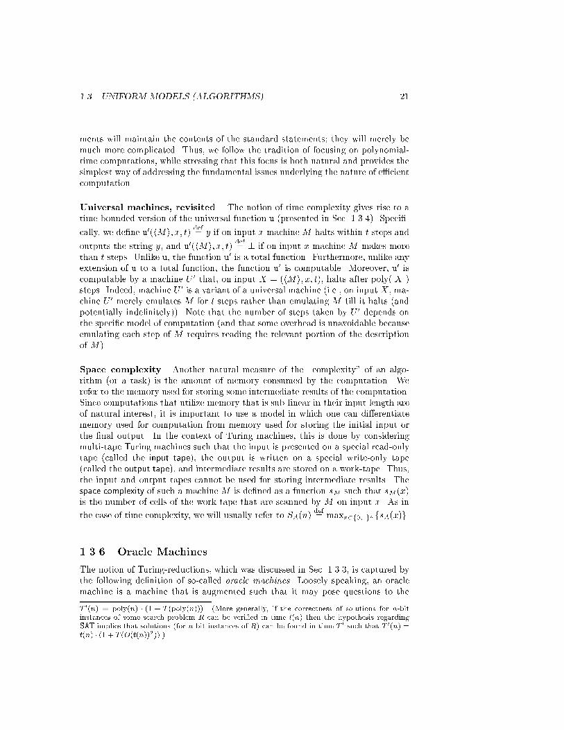
1.3. UNIFORM MODELS (ALGORITHMS) 21ments will maintain the contents of the standard statements; they will merely bemuch more complicated. Thus, we follow the tradition of focusing on polynomial-time computations, while stressing that this focus is both natural and provides thesimplest way of addressing the fundamental issues underlying the nature of e�cientcomputation.Universal machines, revisited. The notion of time complexity gives rise to atime-bounded version of the universal function u (presented in Sec. 1.3.4). Speci�-cally, we de�ne u0(hMi; x; t) def= y if on input x machineM halts within t steps andoutputs the string y, and u0(hMi; x; t) def= ? if on input x machine M makes morethan t steps. Unlike u, the function u0 is a total function. Furthermore, unlike anyextension of u to a total function, the function u0 is computable. Moreover, u0 iscomputable by a machine U 0 that, on input X = (hMi; x; t), halts after poly(jX j)steps. Indeed, machine U 0 is a variant of a universal machine (i.e., on input X , ma-chine U 0 merely emulates M for t steps rather than emulating M till it halts (andpotentially inde�nitely)). Note that the number of steps taken by U 0 depends onthe speci�c model of computation (and that some overhead is unavoidable becauseemulating each step of M requires reading the relevant portion of the descriptionof M).Space complexity. Another natural measure of the \complexity" of an algo-rithm (or a task) is the amount of memory consumed by the computation. Werefer to the memory used for storing some intermediate results of the computation.Since computations that utilize memory that is sub-linear in their input length areof natural interest, it is important to use a model in which one can di�erentiatememory used for computation from memory used for storing the initial input orthe �nal output. In the context of Turing machines, this is done by consideringmulti-tape Turing machines such that the input is presented on a special read-onlytape (called the input tape), the output is written on a special write-only tape(called the output tape), and intermediate results are stored on a work-tape. Thus,the input and output tapes cannot be used for storing intermediate results. Thespace complexity of such a machine M is de�ned as a function sM such that sM (x)is the number of cells of the work-tape that are scanned by M on input x. As inthe case of time complexity, we will usually refer to SA(n) def= maxx2f0;1gnfsA(x)g.1.3.6 Oracle MachinesThe notion of Turing-reductions, which was discussed in Sec. 1.3.3, is captured bythe following de�nition of so-called oracle machines. Loosely speaking, an oraclemachine is a machine that is augmented such that it may pose questions to theT 0(n) = poly(n) � (1 + T (poly(n))). (More generally, if the correctness of solutions for n-bitinstances of some search problem R can be veri�ed in time t(n) then the hypothesis regardingSAT implies that solutions (for n-bit instances of R) can be found in time T 0 such that T 0(n) =t(n) � (1 + T (O(t(n))2)).)

22 CHAPTER 1. COMPUTATIONAL TASKS AND MODELSoutside. We consider the case in which these questions, called queries, are answeredconsistently by some function f : f0; 1g� ! f0; 1g�, called the oracle. That is, ifthe machine makes a query q then the answer it obtains is f(q). In such a case, wesay that the oracle machine is given access to the oracle f . For an oracle machineM , a string x and a function f , we denote by Mf (x) the output of M on inputx when given access to the oracle f . (Re-examining the second part of the proofof Theorem 1.5, observe that we have actually described an oracle machine thatcomputes d0 when given access to the oracle d.)The notion of an oracle machine extends the notion of a standard computingdevice (machine), and thus a rigorous formulation of the former extends a formalmodel of the latter. Speci�cally, extending the model of Turing machines, we derivethe following model of oracle Turing machines.De�nition 1.11 (using an oracle):� An oracle machine is a Turing machine with a special additional tape, calledthe oracle tape, and two special states, called oracle invocation and oracle spoke.� The computation of the oracle machine M on input x and access to the oraclef : f0; 1g� ! f0; 1g� is de�ned based on the successive con�guration function.For con�gurations with state di�erent from oracle invocation the next con�g-uration is de�ned as usual. Let be a con�guration in which the machine'sstate is oracle invocation and suppose that the actual contents of the oracletape is q (i.e., q is the contents of the maximal pre�x of the tape that holdsbit values).8 Then, the con�guration following is identical to , except thatthe state is oracle spoke, and the actual contents of the oracle tape is f(q).The string q is called M 's query and f(q) is called the oracle's reply.� The output of the oracle machine M on input x when given oracle access tof is denote Mf (x).We stress that the running time of an oracle machine is the number of steps madeduring its (own) computation, and that the oracle's reply on each query is obtainedin a single step.1.3.7 Restricted ModelsWe mention that restricted models of computation are often mentioned in thecontext of a course on computability, but they will play no role in the current book.One such model is the model of �nite automata, which in some variant coincideswith Turing machines that have space-complexity zero (equiv., constant).In our opinion, the most important motivation for the study of these restrictedmodels of computation is that they provide simple models for some natural (orarti�cial) phenomena. This motivation, however, seems only remotely related to8This �ts the de�nition of the actual initial contents of a tape of a Turing machine (cf.Sec. 1.3.2). A common convention is that the oracle can be invoked only when the machine'shead resides at the left-most cell of the oracle tape.

1.4. NON-UNIFORM MODELS (CIRCUITS AND ADVICE) 23the study of the complexity of various computational tasks, which calls for the con-sideration of general models of computation and the evaluation of the complexityof computation with respect to such models.Teaching note: Indeed, we reject the common coupling of computability theory withthe theory of automata and formal languages. Although the historical links betweenthese two theories (at least in the West) can not be denied, this fact cannot justifycoupling two fundamentally di�erent theories (especially when such a coupling promotesa wrong perspective on computability theory). Thus, in our opinion, the study of anyof the lower levels of Chomsky's Hierarchy [15, Chap. 9] should be decoupled from thestudy of computability theory (let alone the study of complexity theory).1.4 Non-Uniform Models (Circuits and Advice)In the current book, we only use non-uniform models of computation as a source ofsome natural computational problems (cf. Sec. 4.3.1). We mention, however, thatthese models are typically considered for other purposes (see a brief discussionbelow).By a non-uniform model of computation we mean a model in which for eachpossible input length a di�erent computing device is considered, while there isno \uniformity" requirement relating devices that correspond to di�erent inputlengths. Furthermore, this collection of devices is in�nite by nature, and (in absenceof a uniformity requirement) this collection may not even have a �nite description.Nevertheless, each device in the collection has a �nite description. In fact, therelationship between the size of the device (resp., the length of its description) andthe length of the input that it handles will be of major concern.Non-uniform models of computation are considered either towards the devel-opment of lower-bound techniques or as providing simpli�ed upper bounds on theability of e�cient algorithms.9 In both cases, the uniformity condition is eliminatedin the interest of simplicity and with the hope (and belief) that nothing substantialis lost as far as the issues at hand are concerned. In the context of developing lower-bound, the hope is that the �niteness of all parameters (i.e., the input length andthe device's description) will allow for the application of combinatorial techniquesto analyze the limitations of certain settings of parameters.We will focus on two related models of non-uniform computing devices: Booleancircuits (Sec. 1.4.1) and \machines that take advice" (Sec. 1.4.2). The former modelis more adequate for the study of the evolution of computation (i.e., development oflower-bound techniques), whereas the latter is more adequate for modeling purposes(e.g., limiting the ability of e�cient algorithms).9Advanced comment: The second case refers mainly to e�cient algorithms that are givena pair of inputs (of (polynomially) related length) such that these algorithms are analyzed withrespect to �xing one input (arbitrarily) and varying the other input (typically, at random). Typicalexamples include the context of de-randomization (cf. [13, Sec. 8.3]) and the setting of zero-knowledge (cf. [13, Sec. 9.2]).

24 CHAPTER 1. COMPUTATIONAL TASKS AND MODELSTeaching note: In the context of this book, non-uniform models of computation will(only) be used for giving rise to natural computational problems (e.g., the satis�abilityof Boolean Circuits (cf. Sec. 1.4.1) and Formulae (cf. Sec. 1.4.3)). This use provides aconcrete motivation to the study of the current section; furthermore, we believe thatsome familiarity with the non-uniform models is bene�cial per se.1.4.1 Boolean CircuitsThe most popular model of non-uniform computation is the one of Boolean circuits.Historically, this model was introduced for the purpose of describing the \logicoperation" of real-life electronic circuits. Ironically, nowadays this model providesthe stage for some of the most practically removed studies in complexity theory(which aim at developing methods that may eventually lead to an understandingof the inherent limitations of e�cient algorithms).A Boolean circuit is a directed acyclic graph10 with labels on the vertices, to bediscussed shortly. For sake of simplicity, we disallow isolated vertices (i.e., verticeswith no incoming or outgoing edges), and thus the graph's vertices are of threetypes: sources, sinks, and internal vertices.1. Internal vertices are vertices having incoming and outgoing edges (i.e., theyhave in-degree and out-degree at least 1). In the context of Boolean cir-cuits, internal vertices are called gates. Each gate is labeled by a Booleanoperation, where the operations that are typically considered are ^, _ and :(corresponding to and, or and neg). In addition, we require that gates la-beled : have in-degree 1. The in-degree of ^-gates and _-gates may be anynumber greater than zero, and the same holds for the outdegree of any gate.2. The graph sources (i.e., vertices with no incoming edges) are called inputterminals. Each input terminal is labeled by a natural number (which is tobe thought of the index of an input variable). (For sake of de�ning formulae(see Sec. 1.4.3), we allow di�erent input terminals to be labeled by the samenumber.)113. The graph sinks (i.e., vertices with no outgoing edges) are called output ter-minals, and we require that they have in-degree 1. Each output terminal islabeled by a natural number such that if the circuit has m output terminalsthen they are labeled 1; 2; :::;m. That is, we disallow di�erent output ter-minals to be labeled by the same number, and insist that the labels of theoutput terminals are consecutive numbers. (Indeed, the labels of the outputterminals will correspond to the indices of locations in the circuit's output.)For sake of simplicity, we also mandate that the labels of the input terminals areconsecutive numbers.1210See Appendix A.1.11This is not needed in case of general circuits, because we can just feed outgoing edges of thesame input terminal to many gates. Note, however, that this is not allowed in case of formulae,

1.4. NON-UNIFORM MODELS (CIRCUITS AND ADVICE) 251 2

1 2

0

4 3

and and

and

and

oror

negneg neg

Figure 1.2: A circuit computing f(x1; x2; x3; x4) = (x1 � x2; x1 ^ :x2 ^ x4).A Boolean circuit with n di�erent input labels and m output terminals induces(and indeed computes) a function from f0; 1gn to f0; 1gm de�ned as follows. Forany �xed string x 2 f0; 1gn, we iteratively de�ne the value of vertices in the circuitsuch that the input terminals are assigned the corresponding bits in x = x1 � � �xnand the values of other vertices are determined in the natural manner. That is:� An input terminal with label i 2 f1; :::; ng is assigned the ith bit of x (i.e.,the value xi).� If the children of a gate (of in-degree d) that is labeled ^ have values v1; v2; :::; vd,then the gate is assigned the value ^di=1vi. The value of a gate labeled _ (or :)is determined analogously.Indeed, the hypothesis that the circuit is acyclic implies that the followingnatural process of determining values for the circuit's vertices is well-de�ned:As long as the value of some vertex is undetermined, there exists a vertexsuch that its value is undetermined but the values of all its children aredetermined. Thus, the process can make progress, and terminates when thevalues of all vertices (including the output terminals) are determined.The value of the circuit on input x (i.e., the output computed by the circuit oninput x) is y = y1 � � � ym, where yi is the value assigned by the foregoing processwhere all non-sinks are required to have out-degree exactly 1.12This convention slightly complicates the construction of circuits that ignore some of the inputvalues. Speci�cally, we use arti�cial gadgets that have incoming edges from the correspondinginput terminals, and compute an adequate constant. To avoid having this constant as an outputterminal, we feed it into an auxiliary gate such that the value of the latter is determined by theother incoming edge (e.g., a constant 0 fed into an _-gate). See example of dealing with x3 inFigure 1.2.

26 CHAPTER 1. COMPUTATIONAL TASKS AND MODELSto the output terminal labeled i. We note that there exists a polynomial-timealgorithm that, given a circuit C and a corresponding input x, outputs the value ofC on input x. This algorithm determines the values of the circuit's vertices, goingfrom the circuit's input terminals to its output terminals.We say that a family of circuits (Cn)n2N computes a function f : f0; 1g� ! f0; 1g�if for every n the circuit Cn computes the restriction of f to strings of length n. Inother words, for every x 2 f0; 1g�, it must hold that Cjxj(x) = f(x).Bounded and unbounded fan-in. One is often interested in circuits in whicheach gate has at most two incoming edges. In this case, the types of (two-argument)Boolean operations that we allow is immaterial (as long as we consider a \fullbasis" of such operations; i.e., a set of operations that can implement any othertwo-argument Boolean operation). Such circuits are called circuits of bounded fan-in. In contrast, other studies are concerned with circuits of unbounded fan-in, whereeach gate may have an arbitrary number of incoming edges. Needless to say, inthe case of circuits of unbounded fan-in, the choice of allowed Boolean operationsis important and one focuses on operations that are \uniform" (across the numberof operants; e.g., ^ and _).Circuit size as a complexity measure. The size of a circuit is the number ofits edges. When considering a family of circuits (Cn)n2N that computes a functionf : f0; 1g� ! f0; 1g�, we are interested in the size of Cn as a function of n.Speci�cally, we say that this family has size complexity s : N ! N if for every n thesize of Cn is s(n). The circuit complexity of a function f , denoted sf , is the in�mumof the size complexity of all families of circuits that compute f . Alternatively, foreach n we may consider the size of the smallest circuit that computes the restrictionof f to n-bit strings (denoted fn), and set sf (n) accordingly. We stress that non-uniformity is implicit in this de�nition, because no conditions are made regardingthe relation between the various circuits used to compute the function on di�erentinput lengths.13On the circuit complexity of functions. We highlight some simple facts re-garding the circuit complexity of functions. These facts are in clear correspondenceto facts regarding Kolmogorov Complexity mentioned in Sec. 1.3.4, and establishingthem is left as an exercise (see Exercise 1.10).1. Most importantly, any Boolean function can be computed by some familyof circuits, and thus the circuit complexity of any function is well-de�ned.Furthermore, each function has at most exponential circuit complexity.2. Some functions have polynomial circuit complexity. In particular, any func-tion that has time complexity t (i.e., is computed by an algorithm of time13Advanced comment: We also note that, in contrast to Footnote 6, the circuit model andthe (circuit size) complexity measure support the notion of an optimal computing device: eachfunction f has a unique size complexity sf (and not merely upper- and lower-bounds on itscomplexity).

1.4. NON-UNIFORM MODELS (CIRCUITS AND ADVICE) 27complexity t) has circuit complexity poly(t). Furthermore, the correspond-ing circuit family is uniform (in a natural sense to be discussed in the nextparagraph).3. Almost all Boolean functions have exponential circuit complexity. Speci�-cally, the number of functions mapping f0; 1gn to f0; 1g that can be computedby some circuit of size s is smaller than s2s.Note that the �rst fact implies that families of circuits can compute functions thatare uncomputable by algorithms. Furthermore, this phenomenon occurs also whenrestricting attention to families of polynomial-size circuits. See further discussionin Sec. 1.4.2.Uniform families. A family of polynomial-size circuits (Cn)n2N is called uniformif given n one can construct the circuit Cn in poly(n)-time. Note that if a functionis computable by a uniform family of polynomial-size circuits then it is computableby a polynomial-time algorithm. This algorithm �rst constructs the adequate cir-cuit (which can be done in polynomial-time by the uniformity hypothesis), andthen evaluate this circuit on the given input (which can be done in time that ispolynomial in the size of the circuit).Note that limitations on the computing power of arbitrary families of polynomial-size circuits certainly hold for uniform families (of polynomial-size circuits), whichin turn yield limitations on the computing power of polynomial-time algorithms.Thus, lower-bounds on the circuit-complexity of functions yield analogous lower-bounds on their time-complexity. Furthermore, as is often the case in mathematicsand science, disposing of an auxiliary condition that is not well-understood (i.e.,uniformity) may turn out fruitful. Indeed, this has occured in the study of classesof restricted circuits, which is reviewed in Sec. 1.4.3.1.4.2 Machines That Take AdviceGeneral (non-uniform) circuit families and uniform circuit families are two extremeswith respect to the \amounts of non-uniformity" in the computing device. Intu-itively, in the former, non-uniformity is only bounded by the size of the device,whereas in the latter the amounts of non-uniformity is zero. Here we consider amodel that allows to decouple the size of the computing device from the amountof non-uniformity, which may range from zero to the device's size. Speci�cally, weconsider algorithms that \take a non-uniform advice" that depends only on theinput length. The amount of non-uniformity will be de�ned to equal the length ofthe corresponding advice (as a function of the input length).De�nition 1.12 (taking advice): We say that algorithm A computes the functionf using advice of length ` : N ! N if there exists an in�nite sequence (an)n2N suchthat1. For every x 2 f0; 1g�, it holds that A(ajxj; x) = f(x).2. For every n 2 N , it holds that janj = `(n).

28 CHAPTER 1. COMPUTATIONAL TASKS AND MODELSThe sequence (an)n2N is called the advice sequence.Note that any function having circuit complexity s can be computed using adviceof length O(s log s), where the log factor is due to the fact that a graph with vvertices and e edges can be described by a string of length 2e log2 v. Note that themodel of machines that use advice allows for some sharper bounds than the onesstated in Sec. 1.4.1: every function can be computed using advice of length ` suchthat `(n) = 2n, and some uncomputable functions can be computed using adviceof length 1.Theorem 1.13 (the power of advice): There exist functions that can be computedusing one-bit advice but cannot be computed without advice.Proof: Starting with any uncomputable Boolean function f : N ! f0; 1g, considerthe function f 0 de�ned as f 0(x) = f(jxj). Note that f is Turing-reducible to f 0 (e.g.,on input nmake any n-bit query to f 0, and return the answer).14 Thus, f 0 cannot becomputed without advice. On the other hand, f 0 can be easily computed by usingthe advice sequence (an)n2N such that an = f(n); that is, the algorithm merelyoutputs the advice bit (and indeed ajxj = f(jxj) = f 0(x), for every x 2 f0; 1g�).1.4.3 Restricted ModelsThe model of Boolean circuits (cf. Sec. 1.4.1) allows for the introduction of manynatural subclasses of computing devices. Following is a laconic review of a fewof these subclasses. (For further detail regarding the study of these subclasses,the interested reader is referred to [1].) Since we shall refer to various types ofBoolean formulae in the rest of this book, we suggest not to skip the following twoparagraphs.Boolean formulae. In (general) Boolean circuits the non-sink vertices are al-lowed arbitrary out-degree. This means that the same intermediate value can bere-used without being re-computed (and while increasing the size complexity byonly one unit). Such \free" re-usage of intermediate values is disallowed in Booleanformulae, which are formally de�ned as Boolean circuits in which all non-sink ver-tices have out-degree 1. This means that the underlying graph of a Boolean formulais a tree (see xA.2), and it can be written as a Boolean expression over Booleanvariables by traversing this tree (and registering the vertices' labels in the order tra-versed). Indeed, we have allowed di�erent input terminals to be assigned the samelabel in order to allow formulae in which the same variable occurs multiple times.As in case of general circuits, one is interested in the size of these restricted circuits(i.e., the size of families of formulae computing various functions). We mention thatquadratic lower bounds are known for the formula size of simple functions (e.g.,parity), whereas these functions have linear circuit complexity. This discrepancyis depicted in Figure 1.3.14Indeed, this Turing-reduction is not e�cient (i.e., it runs in exponential time in jnj = log2 n),but this is immaterial in the current context.

1.4. NON-UNIFORM MODELS (CIRCUITS AND ADVICE) 291 n

of x .... x1 n

of x .... x1 n

of x .... x2n

of x ...xn+1 2n

of x ...xn+12n

of x ...xn+1

PARITY PARITY PARITY PARITY PARITY PARITY

and

oror

andand and

neg neg neg neg

Figure 1.3: Recursive construction of parity circuits and formulae.Formulae in CNF and DNF. A restricted type of Boolean formulae consistsof formulae that are in conjunctive normal form (CNF). Such a formula consists ofa conjunction of clauses, where each clause is a disjunction of literals each beingeither a variable or its negation. That is, such formulae are represented by layeredcircuits of unbounded fan-in in which the �rst layer consists of neg-gates thatcompute the negation of input variables, the second layer consist of or-gates thatcompute the logical-or of subsets of inputs and negated inputs, and the third layerconsists of a single and-gate that computes the logical-and of the values computedin the second layer. Note that each Boolean function can be computed by a familyof CNF formulae of exponential size (see Exercise 1.12), and that the size of CNFformulae may be exponentially larger than the size of ordinary formulae computingthe same function (e.g., parity). For a constant k, a formula is said to be in k-CNF if its CNF has disjunctions of size at most k. An analogous restricted typeof Boolean formulae refers to formulae that are in disjunctive normal form (DNF).Such a formula consists of a disjunction of a conjunctions of literals, and when eachconjunction has at most k literals we say that the formula is in k-DNF.Constant-depth circuits. Circuits have a \natural structure" (i.e., their struc-ture as graphs). One natural parameter regarding this structure is the depth of acircuit, which is de�ned as the longest directed path from any source to any sink. Ofspecial interest are constant-depth circuits of unbounded fan-in. We mention thatsub-exponential lower bounds are known for the size of such circuits that computea simple function (e.g., parity).Monotone circuits. The circuit model also allows for the consideration of mono-tone computing devices: a monotone circuit is one having only monotone gates(e.g., gates computing ^ and _, but no negation gates (i.e., :-gates)). Needlessto say, monotone circuits can only compute monotone functions, where a functionf : f0; 1gn ! f0; 1g is called monotone if for any x � y it holds that f(x) � f(y)(where x1 � � �xn � y1 � � � yn if and only if for every bit position i it holds thatxi � yi). One natural question is whether, as far as monotone functions are con-

30 CHAPTER 1. COMPUTATIONAL TASKS AND MODELScerned, there is a substantial loss in using only monotone circuits. The answer isyes: there exist monotone functions that have polynomial circuit complexity butrequire sub-exponential size monotone circuits.1.5 Complexity ClassesComplexity classes are sets of computational problems. Typically, such classes arede�ned by �xing three parameters:1. A type of computational problems (see Section 1.2). Indeed, most classes referto decision problems, but classes of search problems, promise problems, andother types of problems are also considered.2. A model of computation, which may be either uniform (see Section 1.3) ornon-uniform (see Section 1.4).3. A complexity measure and a limiting function (or a set of functions), whichput together limit the class of computations of the previous item; that is,we refer to the class of computations that have complexity not exceeding thespeci�ed function (or set of functions). For example, in Sec. 1.3.5, we men-tioned time-complexity and space-complexity, which apply to any uniformmodel of computation. We also mentioned polynomial-time computations,which are computations in which the time-complexity (as a function) doesnot exceed some polynomial (i.e., is a member of the set of polynomial func-tions).The most common complexity classes refer to decision problems, and are sometimesde�ned as classes of sets rather than classes of the corresponding decision problems.That is, one often says that a set S � f0; 1g� is in the class C rather than sayingthat the problem of deciding membership in S is in the class C. Likewise, one talksof classes of relations rather than classes of the corresponding search problems (i.e.,saying that R � f0; 1g��f0; 1g� is in the class C means that the search problem ofR is in the class C).ExercisesExercise 1.1 Prove that any function that can be computed by a Turing machinecan be computed by a machine that never moves left of the end of the tape.Guideline: Modify the original machine by using a \marking" of the leftmost cell of thetape. Needless to say, this marking corresponds to an extension of the tape's symbols.Exercise 1.2 (single-tape versus multi-tape Turing machines) Prove thata function can be computed by a single-tape Turing machine if and only if it iscomputable by a multi-tape (e.g., two-tape) Turing machine.Guideline: The emulation of the multi-tape Turing machine on a single-tape machine isbased on storing all the original tapes on a single tape such that the ith cell of the single

1.5. COMPLEXITY CLASSES 31tape records the contents of the ith cell of each of the original tapes. In addition, the ithcell of the single tape records an indication as to which of the original heads reside inthe ith cell of the corresponding original tape. To emulate a single step of the originalmachine, the new machine scans its tape, �nds all original head locations, and retrievesthe corresponding cell contents. Based on this information, the emulating machine e�ectsthe corresponding step (according to the original transition function), by modifying its(single) tape's contents in an analogous manner.Exercise 1.3 (computing the sum of natural numbers) Prove that a Tur-ing machine can add natural numbers; that is, outline a (multi-tape) Turing ma-chine that on input a pair of integers (in binary representation), outputs their sum.Speci�cally, show that the straightforward addition algorithm can be implementedin linear time by a multi-tape Turing machine.Guideline: A straightforward implementation of addition on a two-tape Turing machinestarts by copying the two (input) integers to the second tape such that the ith leastsigni�cant bits of both integers resides in the same cell.Exercise 1.4 (Turing machines vs abstract RAM) Prove that abstract RAMscan be emulated by a Turing machine.Guideline: Note that, during the emulation (of the abstract RAM), we only need tohold the input, the contents of all registers, and the contents of the memory cells thatwere accessed during the computation. Thus, at each time, the Turning machine's tapecontains a list of the RAM's memory cells that were accessed so far as well as their currentcontents. When we emulate a RAM instruction, we �rst check whether the relevant RAMcell appears on this list, and augment the list by a corresponding entry or modify thisentry as needed.Exercise 1.5 (Rice's Theorem (Theorem 1.6)) Let F and SF be as in The-orem 1.6. Present a Turing-reduction of d to SF .Guideline: Let f? denote the function that is unde�ned on all inputs. Assume, withoutloss of generality, that f? 62 F , let f1 denote an arbitrary function in F , and let M1 bean arbitrary �x machine that computes f1. Then, the reduction maps an input hMi ford into an input hM 0i for SF such that on input x machine M 0 operates as follows:1. First, machine M 0 emulates M on input hMi.2. If M halts (in Step 1), then M 0 emulates M1(x), and outputs whatever it does.Note that the mapping from hMi to hM 0i is easily computable (by augmenting M withthe �xed machineM1). If h(hMi) = 1 then machineM 0 reaches Step 2, and thusM 0(x) =f1(x), which in turn implies hMi 2 SF . On the other hand, if h(hMi) = 0 then machineM 0 remains stuck in Step 1, and thus M 0 does not halt on any x, which in turn implieshMi 62 SF (because M 0 computes f?).Exercise 1.6 (Post Correspondence Problem (Theorem 1.7)) Present a Turing-reduction of h to the Post Correspondence Problem, denoted PCP. Furthermore, usea reduction that maps an instance (hMi; x) of h to a pair of sequences ((�1; :::; �k); (�1; :::; �k))

32 CHAPTER 1. COMPUTATIONAL TASKS AND MODELSsuch that only �1 and �1 depend on x, whereas k as well as the other strings dependonly on M .Guideline: Consider a a modi�ed version of the Post Correspondence Problem, denotedMPCP, in which the �rst index in the solution sequence must equal 1 (i.e., i1 = 1). Reduce hto MPCP, and next reduce MPCP to PCP. The main reduction (i.e., of h to MPCP) maps (hMi; x)to ((�1; :::; �k); (�1; :::; �k)) such that a solution sequence (i.e., i1; :::; i` s.t. �i1 � � ��i` =�1 � � � �i`) yields a full description of the computation of M on input x (i.e., the sequenceof all instantaneous con�gurations in this computation). Speci�cally, �1 will describe theinitial con�guration of M on input x, whereas �1 will be essentially empty (except for adelimiter, denoted #, which is also used at the beginning and at the end of �1). Assumingthat the set of tape-symbols and the set of states of M are disjoint (i.e., � \ Q = ;),con�gurations will be described as sequences over their union (i.e., sequences over �\Q,where # 62 � \Q). Other pairs (�i; �i) include� For every tape-symbol �, we shall have �i = �i = � (for some i). We shall alsohave �i = �i = # (for some i). Such pairs re ect the preservation of the tape'scontents (whenever the head location is not present at the current cell).� For every non-halting state q and every transition regarding q, we shall have a pairre ecting this transition. For example, if the transition function maps (q; �) to(q0; �0;+1), then we have �i = q� and �i = �0q0 (for some i). For left movement(i.e., if the transition function maps (q; �) to (q0; �0;�1)) we have �i = �q� and�i = q0��0. Assuming that blank symbols (i.e., ) are only written to the left ofother black symbols (and when moving left), if the transition function maps (q; �)to (q0; ;�1), then we have �i = �q� and �i = q0� (rather than �i = q0� ).� Assuming that the machine halts in state p only when it resides in the leftmost cell(and after writing blanks in all cells), we have �i = p ## and �i = # (for some i).Note that in a solution sequence i1; :::; i` such that �i1 � � ��i` = �1 � � � �i` , for every t < `it holds that �i1 � � � �it is a pre�x of �i1 � � ��it such that the latter contains exactlycon�guration less than the former. The relations between the pairs (�i; �i) guaranteethat these pre�ces are pre�ces of the sequence of all instantaneous con�gurations in thecomputation of M on input x, and a solution can be completed only if this computationhalts. For details see [15, Sec. 8.5] or [29, Sec. 5.2].Exercise 1.7 (total functions extending the universal function) Let u bethe function computed by any universal machine (for a �xed reasonable modelof computation). Prove that any extension of u to a total function (i.e., any totalfunction u that agrees with the partial function u on all the inputs on which thelatter is de�ned) is uncomputable.Guideline: The claim is easy to prove for the special case of the total function u thatextends u such that the special symbol ? is assigned to inputs on which u is unde�ned(i.e., u(hMi; x) def= ? if u is not de�ned on (hMi; x) and u(hMi; x) def= u(hMi; x) otherwise).In this case h(hMi; x) = 1 if and only if u(hMi; x) 6= ?, and so the halting function h isTuring-reducible to u. In the general case, we may adapt the proof of Theorem 1.5 byusing the fact that, for any machineM that halts on every input, it holds that u(hMi; x) =u(hMi; x) for every x (and in particular for x = hMi).

1.5. COMPLEXITY CLASSES 33Exercise 1.8 (uncomputability of Kolmogorov Complexity) Prove that Kol-mogorov Complexity function, denoted K, is uncomputable.Guideline: Consider, for every integer t, the string st that is de�ned as the lexicograph-ically �rst string of Kolmogorov Complexity exceeding t (i.e., st def= mins2f0;1g�fK(s) >tg). Note that st is well de�ned and has length at most t. Assuming thatK is computable,we reach a contradiction by noting that st has description length O(1) + log2 t (becauseit may be described by combining a �xed machine that computes K with the integer t).Exercise 1.9 (single-tape vs two-tape Turing machines, revisited) Prove thatdeciding membership in the set fxx : x 2 f0; 1g�g requires quadratic-time ona single-tape Turing machine. Note that this decision problem can be solved inlinear-time on a two-tape Turing machine.Guideline: Proving the former fact is quite non-trivial. One proof is by a \reduction"from a communication complexity problem [18, Sec. 12.2]. Intuitively, a single-tape Turingmachine that decides membership in the aforementioned set can be viewed as a channel ofcommunication between the two parts of the input. Speci�cally, focusing our attention oninputs of the form y0nz0n, for y; z 2 f0; 1gn, note that each time that the machine passesfrom the one part to the other part it carries O(1) bits of information (in its internalstate) while making at least n steps. The proof is completed by invoking the linear lower-bound on the communication complexity of the (two-argument) identity function (i.e,id(y; z) = 1 if y = z and id(y; z) = 0 otherwise); cf. [18, Chap. 1].Exercise 1.10 (on the circuit complexity of functions) Prove the followingfacts:1. The circuit complexity of any Boolean function is at most exponential.Guideline: fn : f0; 1gn ! f0; 1g can be computed by a circuit of size O(n2n)that implements a look-up table.2. Some functions have polynomial circuit complexity. In particular, any func-tion that has time complexity t (i.e., is computed by an algorithm of timecomplexity t), has circuit complexity poly(t). Furthermore, the correspond-ing circuit family is uniform.Guideline: Consider a Turing machine that computes the function, and considerits computation on a generic n-bit long input. The corresponding computation canbe emulated by a circuit that consists of t(n) layers such that each layer representsan instantaneous con�guration of the machine, and the relation between consecutivecon�gurations is captured by (\uniform") local gadgets in the circuit. For furtherdetails see the proof of Theorem 4.5, which presents a similar emulation.3. Almost all Boolean functions have exponential circuit complexity. Speci�-cally, the number of functions mapping f0; 1gn to f0; 1g that can be computedby some circuit of size s is smaller than s2s.Guideline: Show that, without loss of generality, we may consider circuits ofbounded fan-in. The number of such circuits having v vertices and s edges is atmost �2 � �v2�+ v�s.

34 CHAPTER 1. COMPUTATIONAL TASKS AND MODELSExercise 1.11 (the class P=poly) We denote by P=` the class of decision prob-lems that can be solved in polynomial-time with advice of length `, and by P=polythe union of P=p taken over all polynomials p. Prove that a decision problem is inP=poly if and only if it has polynomial circuit-size complexity.Guideline: Suppose that a problem can be solved by a polynomial-time algorithmA using the polynomially bounded advice sequence (an)n2N. We obtain a family ofpolynomial-size circuits that solves the same problem by observing that the computa-tion of A(ajxj; x) can be emulated by a circuit of poly(jxj)-size, which incorporates ajxjand is given x as input. That is, we construct a circuit Cn such that Cn(x) = A(an; x)holds for every x 2 f0; 1gn (analogously to the way Cx is constructed in the proof ofTheorem 4.5, where it holds that Cx(y) = MR(x; y) for every y of adequate length). Onthe other hand, given a family of polynomial-size circuits, we obtain a polynomial-timeadvice-taking machine that emulates this family when using advice that provide the de-scription of the relevant circuits. (Indeed, we use the fact that a circuit of size s can bedescribed by a string of length O(s log s).)Exercise 1.12 Prove that every Boolean function can be computed by a familyof DNF (resp., CNF) formulae of exponential size.Guideline: For any a 2 f0; 1gn, consider the function �a : f0; 1gn ! f0; 1g such that�a(x) = 1 if x = a and �a(x) = 0 otherwise. Note that any function �a can be computed bya single conjunction of n literals, and that any Boolean function f : f0; 1gn ! f0; 1g canbe written as Wa:f(a)=1 �a. A corresponding CNF formula can be obtained by applyingde-Morgan's Law to the DNF obtained for :f .

Chapter 2The P versus NP QuestionOur daily experience is that it is harder to solve problems than it is to check thecorrectness of solutions to these problems. Is this experience merely a coincidenceor does it represent a fundamental fact of life (or a property of the world)? This isthe essence of the P versus NP Question, where P represents search problems thatare e�ciently solvable and NP represents search problems for which solutions canbe e�ciently checked.Another natural question captured by the P versus NP Question is whetherproving theorems is harder that verifying the validity of these proofs. In otherwords, the question is whether deciding membership in a set is harder than beingconvinced of this membership by an adequate proof. In this case, P representsdecision problems that are e�ciently solvable, whereas NP represents sets that havee�ciently checkable proofs of membership.These two formulations of the P versus NP Question are rigorously presentedand discussed in Sections 2.1 and 2.2, respectively. The equivalence of these for-mulations is shown in Section 2.3, and the common belief that P is di�erent fromNP is further discussed in Section 2.6. We start by recalling the notion of e�cientcomputation.Teaching note: Most students have heard of P and NP before, but we suspect thatmany of them have not obtained a good explanation of what the P-vs-NP Questionactually represents. This unfortunate situation is due to using the standard techni-cal de�nition of NP (which refers to the �ctitious and confusing device called a non-deterministic polynomial-time machine). Instead, we advocate the use of slightly morecumbersome de�nitions, sketched in the foregoing paragraphs (and elaborated in Sec-tions 2.1 and 2.2), which clearly capture the fundamental nature of NP.The notion of e�cient computation. Recall that we associate e�cient com-putation with polynomial-time algorithms.1 This association is justi�ed by thefact that polynomials are moderately growing functions and the set of polynomials1Advanced comment: In this book, we consider deterministic (polynomial-time) algorithmsas the basic model of e�cient computation. A more liberal view, which includes also probabilistic35

36 CHAPTER 2. THE P VERSUS NP QUESTIONis closed under operations that correspond to natural composition of algorithms.Furthermore, the class of polynomial-time algorithms is independent of the speci�cmodel of computation, as long as the latter is \reasonable" (cf. the Cobham-Edmonds Thesis). Both issues are discussed in Sec. 1.3.5.Advanced note on the representation of problem instances. As noted inSec. 1.2.3, many natural (search and decision) problems are captured more natu-rally by the terminology of promise problems (cf. Section 5.1), where the domain ofpossible instances is a subset of f0; 1g� rather than f0; 1g� itself. For example, com-putational problems in graph theory presume some simple encoding of graphs asstrings, but this encoding is typically not onto (i.e., not all strings encode graphs),and thus not all strings are legitimate instances. However, in these cases, the setof legitimate instances (e.g., encodings of graphs) is e�ciently recognizable (i.e.,membership in it can be decided in polynomial-time). Thus, arti�cially extendingthe set of instances to the set of all possible strings (and allowing trivial solutionsfor the corresponding dummy instances) does not change the complexity of theoriginal problem. We further discuss this issue in Section 5.1.2.1 The Search Version: Finding Versus Check-ingTeaching note: Complexity theorists are so accustomed to focus on decision prob-lems that they seem to forget that search problems are at least as natural as decisionproblems. Furthermore, to many non-experts, search problems may seem even morenatural than decision problems: Typically, people seek solutions more often than theypause to wonder whether or not solutions exist. Thus, we recommend starting witha formulation of the P-vs-NP Question in terms of search problems. Admittingly, thecost is more cumbersome formulations, but it is more than worthwhile.Teaching note: In order to re ect the importance of the search version as well asallow less cumbersome formulations, we chose to introduce notations for the two searchclasses corresponding to P and NP: these classes are denoted PF and PC (standingfor Polynomial-time Find and Polynomial-time Check, respectively). The teacher mayprefer using notations and terms that are more evocative of P and NP (such as P-searchand NP-search), and actually we also do so in some motivational discussions. (Still, inour opinion, in the long run, the students and the �eld may be served better by usingstandard-looking notations.)Much of computer science is concerned with solving various search problems (as inDe�nition 1.1). Examples of such problems include �nding a solution to a system oflinear (or polynomial) equations, �nding a prime factor of a given integer, �nding a(polynomial-time) algorithms (see [23] or [13, Chap. 6]). We stress that the most importantfacts and questions that are addressed in the current book hold also with respect to probabilisticpolynomial-time algorithms.

2.1. THE SEARCH VERSION: FINDING VERSUS CHECKING 37spanning tree in a graph, �nding a short traveling salesman tour in a metric space,and �nding a scheduling of jobs to machines such that various constraints aresatis�ed. Furthermore, search problems correspond to the daily notion of \solvingproblems" and are thus of natural general interest. In the current section, we willconsider the question of which search problems can be solved e�ciently.One type of search problems that cannot be solved e�ciently consists of searchproblems for which the solutions are too long in terms of the problem's instances.In such a case, merely typing the solution amounts to an activity that is deemedine�cient. Thus, we focus our attention on search problems that are not in thisclass. That is, we consider only search problems in which the length of the solutionis bounded by a polynomial in the length of the instance. Recalling that searchproblems are associated with binary relations (see De�nition 1.1), we focus ourattention on polynomially bounded relations.De�nition 2.1 (polynomially bounded relations): We say that R � f0; 1g� �f0; 1g� is polynomially-bounded if there exists a polynomial p such that for every(x; y) 2 R it holds that jyj � p(jxj).Recall that (x; y) 2 R means that y is a solution to the problem instance x, whereR represents the problem itself. For example, in the case of �nding a prime factorof a given integer, we refer to a relation R such that (x; y) 2 R if the integer y is aprime factor of the integer x. Likewise, in the case of �nding a spanning tree in agiven graph, we refer to a relation R such that (x; y) 2 R if y is a spanning tree ofthe graph x.For a polynomially bounded relation R it makes sense to ask whether or not,given a problem instance x, one can e�ciently �nd an adequate solution y (i.e.,�nd y such that (x; y) 2 R). The polynomial bound on the length of the solution(i.e., y) guarantees that a negative answer is not merely due to the length of therequired solution.2.1.1 The Class P as a Natural Class of Search ProblemsRecall that we are interested in the class of search problems that can be solved ef-�ciently; that is, problems for which solutions (whenever they exist) can be founde�ciently. Restricting our attention to polynomially bounded relations, we iden-tify the corresponding fundamental class of search problem (or binary relation),denoted PF (standing for \Polynomial-time Find"). (The relationship betweenPF and the standard de�nition of P will be discussed in Sections 2.3 and 3.3.)The following de�nition refers to the formulation of solving search problems pro-vided in De�nition 1.1.De�nition 2.2 (e�ciently solvable search problems):� The search problem of a polynomially bounded relation R � f0; 1g� � f0; 1g�is e�ciently solvable if there exists a polynomial time algorithm A such that,for every x, it holds that A(x) 2 R(x) def= fy : (x; y) 2 Rg if and only if R(x)is not empty. Furthermore, if R(x) = ; then A(x) = ?, indicating that x hasno solution.

38 CHAPTER 2. THE P VERSUS NP QUESTION� We denote by PF the class of search problems that are e�ciently solvable(and correspond to polynomially bounded relations). That is, R 2 PF ifR is polynomially bounded and there exists a polynomial time algorithm thatgiven x �nds y such that (x; y) 2 R (or asserts that no such y exists).Note that R(x) denotes the set of valid solutions for the problem instance x. Thus,the solver A is required to �nd a valid solution (i.e., satisfy A(x) 2 R(x)) wheneversuch a solution exists (i.e., R(x) is not empty). On the other hand, if the instancex has no solution (i.e., R(x) = ;) then clearly A(x) 62 R(x). The extra condition(also made in De�nition 1.1) requires that in this case A(x) = ?. Thus, algorithmA always outputs a correct answer, which is a valid solution in the case that sucha solution exists and otherwise provides an indication that no solution exists.We have de�ned a fundamental class of problems, and we do know of manynatural problems in this class (e.g., solving linear equations over the rationals,�nding a perfect matching in a graph, etc).2 However, we must admit that wedo not have a good understanding regarding the actual contents of this class (i.e.,we are unable to characterize many natural problems with respect to membershipin this class). This situation is quite common in complexity theory, and seems tobe a consequence of the fact that complexity classes are de�ned in terms of the\external behavior" (of potential algorithms) rather than in terms of the \internalstructure" (of the problem). Turning back to PF , we note that, while it containsmany natural search problems, there are also many natural search problems thatare not known to be in PF . A natural class containing a host of such problems ispresented next.2.1.2 The Class NP as Another Natural Class of SearchProblemsNatural search problems have the property that valid solutions (for them) can bee�ciently recognized. That is, given an instance x of the problem R and a candidatesolution y, one can e�ciently determine whether or not y is a valid solution for x(with respect to the problem R; i.e., whether or not y 2 R(x)). The class of all suchsearch problems is a natural class per se, because it is not clear why one should careabout a solution unless one can recognize a valid solution once given. Furthermore,this class is a natural domain of candidates for PF , because the ability to e�cientlyrecognize a valid solution seems to be a natural (albeit not absolute) prerequisitefor a discussion regarding the complexity of �nding such solutions.We restrict our attention again to polynomially bounded relations, and considerthe class of relations for which membership of pairs in the relation can be decidede�ciently. We stress that we consider deciding membership of given pairs of theform (x; y) in a �xed relation R, and not deciding membership of x in the setSR def= fx : R(x) 6= ;g. (The relationship between the following de�nition and thestandard de�nition of NP will be discussed in Sections 2.3{2.5 and 3.3.)2Additional examples include sorting integers, �nding shortest paths in graphs, �nding patternsin strings, and a variety of other tasks that are typically the focus of various courses on algorithms.

2.1. THE SEARCH VERSION: FINDING VERSUS CHECKING 39De�nition 2.3 (search problems with e�ciently checkable solutions):� The search problem of a polynomially bounded relation R � f0; 1g� � f0; 1g�has e�ciently checkable solutions if there exists a polynomial time algorithm Asuch that, for every x and y, it holds that A(x; y) = 1 if and only if (x; y) 2 R.� We denote by PC (standing for \Polynomial-time Check") the class of searchproblems that correspond to polynomially-bounded binary relations that havee�ciently checkable solutions. That is, R 2 PC if the following two conditionshold:1. For some polynomial p, if (x; y) 2 R then jyj � p(jxj).2. There exists a polynomial-time algorithm that given (x; y) determineswhether or not (x; y) 2 R.Note that the algorithm postulated in Item 2 must also handle inputs of the form(x; y) such that jyj > p(jxj). Such inputs, which are evidently not in R (by Item 1),are easy to handle by merely determining jxj; jyj and p(jxj). Thus, the crux ofItem 2 is typically in the case that the input (x; y) satis�es jyj � p(jxj).The class PC contains thousands of natural problems (e.g., �nding a travelingsalesman tour of length that does not exceed a given threshold, �nding the primefactorization of a given composite, �nding a truth assignment that satis�es a givenBoolean formula, etc). In each of these natural problems, the correctness of solu-tions can be checked e�ciently (e.g., given a traveling salesman tour it is easy tocompute its length and check whether or not it exceeds the given threshold).3The class PC is the natural domain for the study of which problems are in PF ,because the ability to e�ciently recognize a valid solution is a natural prerequisitefor a discussion regarding the complexity of �nding such solutions. We warn, how-ever, that PF contains (unnatural) problems that are not in PC (see Exercise 2.1).2.1.3 The P Versus NP Question in Terms of Search Prob-lemsIs it the case that every search problem in PC is in PF? That is, if one cane�ciently check the correctness of solutions with respect to some (polynomially-bounded) relation R, then is it necessarily the case that the search problem of Rcan be solved e�ciently? In other words, if it is easy to check whether or not agiven solution for a given instance is correct, then is it also easy to �nd a solutionto a given instance?If PC � PF then this would mean that whenever solutions to given instancescan be e�ciently checked (for correctness) it is also the case that such solutionscan be e�ciently found (when given only the instance). This would mean that all3In the traveling salesman problem (TSP), the instance is a matrix of distances between citiesand a threshold, and the task is to �nd a tour that passes all cities and covers a total distancethat does not exceed the threshold.

40 CHAPTER 2. THE P VERSUS NP QUESTIONreasonable search problems (i.e., all problems in PC) are easy to solve. Needless tosay, such a situation would contradict the intuitive feeling (and the daily experience)that some reasonable search problems are hard to solve. Furthermore, in such acase, the notion of \solving a problem" would lose its meaning (because �nding asolution will not be signi�cantly more di�cult than checking its validity).On the other hand, if PC nPF 6= ; then there exist reasonable search problems(i.e., some problems in PC) that are hard to solve. This conforms with our basicintuition by which some reasonable problems are easy to solve whereas others arehard to solve. Furthermore, it recon�rms the intuitive gap between the notions ofsolving and checking (asserting that in some cases \solving" is signi�cantly harderthan \checking").As an illustration to the foregoing paragraph, consider various puzzles (e.g.,Jigsaw puzzles, mazes, crossword puzzles, Sudoku puzzles, etc). In each of thesepuzzles checking the correctness of a solution is very easy, whereas �nd a solutionis sometimes extremely hard.2.2 The Decision Version: Proving Versus Veri-fyingAs we shall see in the sequel, the study of search problems (e.g., the PC-vs-PFQuestion) can be \reduced" to the study of decision problems. Since the latterproblems have a less cumbersome terminology, complexity theory tends to focuson them (and maintains its relevance to the study of search problems via the afore-mentioned reduction). Thus, the study of decision problems provides a convenientway for studying search problems. For example, the study of the complexity of de-ciding the satis�ability of Boolean formulae provides a convenient way for studyingthe complexity of �nding satisfying assignments for such formulae.We wish to stress, however, that decision problems are interesting and naturalper se (i.e., beyond their role in the study of search problems). After all, somepeople do care about the truth, and so determining whether certain claims are trueis a natural computational problem. Speci�cally, determining whether a given ob-ject (e.g., a Boolean formula) has some predetermined property (e.g., is satis�able)constitutes an appealing computational problem. The P-vs-NP Question refers tothe complexity of solving such problems for a wide and natural class of propertiesassociated with the class NP. The latter class refers to properties that have \e�-cient proof systems" allowing for the veri�cation of the claim that a given objecthas a predetermined property (i.e., is a member of a predetermined set). Jumpingahead, we mention that the P-vs-NP Question refers to the question of whetherproperties that have e�cient proof systems can also be decided e�ciently (withoutproofs). Let us clarify all these notions.Properties of objects are modeled as subsets of the set of all possible objects (i.e.,a property is associated with the set of objects having this property). For example,the property of being a prime is associated with the set of prime numbers, andthe property of being connected (resp., having a Hamiltonian path) is associated

2.2. THE DECISION VERSION: PROVING VERSUS VERIFYING 41with the set of connected (resp., Hamiltonian) graphs. Thus, we focus on decidingmembership in sets (as in De�nition 1.2). The standard formulation of the P-vs-NP Question refers to the questionable equality of two natural classes of decisionproblems, denoted P and NP (and de�ned in Sec. 2.2.1 and Sec. 2.2.2, respectively).2.2.1 The Class P as a Natural Class of Decision ProblemsNeedless to say, we are interested in the class of decision problems that are e�cientlysolvable. This class is traditionally denoted P (standing for Polynomial-time). Thefollowing de�nition refers to the formulation of solving decision problems (providedin De�nition 1.2).De�nition 2.4 (e�ciently solvable decision problems):� A decision problem S � f0; 1g� is e�ciently solvable if there exists a polyno-mial time algorithm A such that, for every x, it holds that A(x) = 1 if andonly if x 2 S.� We denote by P the class of decision problems that are e�ciently solvable.As in De�nition 2.2, we have de�ned a fundamental class of problems, which con-tains many natural problems (e.g., determining whether or not a given graph isconnected), but we do not have a good understanding regarding its actual contents(i.e., we are unable to characterize many natural problems with respect to mem-bership in this class). In fact, there are many natural decision problems that arenot known to reside in P , and a natural class containing a host of such problemsis presented next. This class of decision problems is denoted NP (for reasons thatwill become evident in Section 2.5).2.2.2 The Class NP and NP-Proof SystemsWe view NP as the class of decision problems that have e�ciently veri�able proofsystems. Loosely speaking, we say that a set S has a proof system if instancesin S have valid proofs of membership (i.e., proofs accepted as valid by the sys-tem), whereas instances not in S have no valid proofs. Indeed, proofs are de�nedas strings that (when accompanying the instance) are accepted by the (e�cient)veri�cation procedure. We say that V is a veri�cation procedure for membershipin S if it satis�es the following two conditions:1. Completeness: True assertions have valid proofs (i.e., proofs accepted as validby V ). Bearing in mind that assertions refer to membership in S, this meansthat for every x 2 S there exists a string y such that V (x; y) = 1 (i.e., Vaccepts y as a valid proof for the membership of x in S).2. Soundness: False assertions have no valid proofs. That is, for every x 62 Sand every string y it holds that V (x; y) = 0, which means that V rejects y asa proof for the membership of x in S.

42 CHAPTER 2. THE P VERSUS NP QUESTIONWe note that the soundness condition captures the \security" of the veri�cationprocedure, that is, its ability not to be fooled (by anything) into proclaiming awrong assertion. The completeness condition captures the \viability" of the veri-�cation procedure, that is, its ability to be convinced of any valid assertion (whenpresented with an adequate proof). We stress that, in general, proof systemsare de�ned in terms of their veri�cation procedures, which must satisfy adequatecompleteness and soundness conditions. Our focus here is on e�cient veri�cationprocedures that utilize relatively short proofs (i.e., proofs that are of length thatis polynomially bounded by the length of the corresponding assertion).4Let us consider a couple of examples before turning to the actual de�nition.Starting with the set of Hamiltonian graphs, we note that this set has a veri�cationprocedure that, given a pair (G; �), accepts if and only if � is a Hamiltonian path inthe graph G. In this case � serves as a proof that G is Hamiltonian. Note that suchproofs are relatively short (i.e., the path is actually shorter than the descriptionof the graph) and are easy to verify. Needless to say, this proof system satis�esthe aforementioned completeness and soundness conditions. Turning to the caseof satis�able Boolean formulae, given a formula � and a truth assignment � , theveri�cation procedure instantiates � (according to �), and accepts if and only ifsimplifying the resulting Boolean expression yields the value true. In this case �serves as a proof that � is satis�able, and the alleged proofs are indeed relativelyshort and easy to verify.De�nition 2.5 (e�ciently veri�able proof systems):� A decision problem S � f0; 1g� has an e�ciently veri�able proof system ifthere exists a polynomial p and a polynomial-time (veri�cation) algorithm Vsuch that the following two conditions hold:1. Completeness: For every x 2 S, there exists y of length at most p(jxj)such that V (x; y) = 1.(Such a string y is called an NP-witness for x 2 S.)2. Soundness: For every x 62 S and every y, it holds that V (x; y) = 0.Thus, x 2 S if and only if there exists y of length at most p(jxj) such thatV (x; y) = 1.In such a case, we say that S has an NP-proof system, and refer to V as itsveri�cation procedure (or as the proof system itself).4Advanced comment: In continuation of Footnote 1, we note that in this chapter we considerdeterministic (polynomial-time) veri�cation procedures, and consequently the completeness andsoundness conditions that we state here are error-less. In contrast, we mention that various typesof probabilistic (polynomial-time) veri�cation procedures as well as probabilistic completenessand soundness conditions are also of interest (see, e.g., [13, Chap. 9]). A common theme thatunderlies both treatments is that e�cient veri�cation is interpreted as meaning veri�cation by aprocess that runs in time that is polynomial in the length of the assertion. In the current chapter,we use the equivalent formulation that considers the running time as a function of the total lengthof the assertion and the proof, but require that the latter has length that is polynomially boundedby the length of the assertion.

2.2. THE DECISION VERSION: PROVING VERSUS VERIFYING 43� We denote by NP the class of decision problems that have e�ciently veri�ableproof systems.We note that the term NP-witness is commonly used.5 In some cases, V (or theset of pairs accepted by V ) is called a witness relation of S. We stress that the sameset S may have many di�erent NP-proof systems (see Exercise 2.3), and that insome cases the di�erence is not arti�cial (see Exercise 2.4).Using De�nition 2.5, it is typically easy to show that natural decision prob-lems are in NP . All that is needed is designing adequate NP-proofs of member-ship, which is typically quite straightforward and natural, because natural decisionproblems are typically phrased as asking about the existence of a structure (orobject) that can be easily veri�ed as valid. For example, SAT is de�ned as the setof satis�able Boolean formulae, which means asking about the existence of satis-fying assignments. Indeed, we can e�ciently check whether a given assignmentsatis�es a given formula, which means that we have (a veri�cation procedure for)an NP-proof system for SAT.Note that for any search problem R in PC, the set of instances that have a so-lution with respect to R (i.e., the set SR def= fx : R(x) 6= ;g) is in NP . Speci�cally,for any R 2 PC, consider the veri�cation procedure V such that V (x; y) def= 1 if andonly if (x; y) 2R, and note that the latter condition can be decided in poly(jxj)-time. Thus, any search problem in PC can be viewed as a problem of searchingfor (e�ciently veri�able) proofs (i.e., NP-witnesses for membership in the set ofinstances having solutions). On the other hand, any NP-proof system gives rise toa natural search problem in PC, that is, the problem of searching for a valid proof(i.e., an NP-witness) for the given instance. (Speci�cally, the veri�cation procedureV yields the search problem that corresponds to R = f(x; y) : V (x; y)=1g.) Thus,S 2 NP if and only if there exists R 2 PC such that S = fx : R(x) 6= ;g.The last paragraph suggests another easy way of showing that natural decisionproblems are in NP : just thinking of the corresponding natural search problem.The point is that natural decision problems (in NP) are phrased as referring towhether a solution exists for the corresponding natural search problem. (For exam-ple, in the case of SAT, the question is whether there exists a satisfying assignmentto given Boolean formula, and the corresponding search problem is �nding suchan assignment.) In all these cases, it is easy to check the correctness of solutions;that is, the corresponding search problem is in PC, which implies that the decisionproblem is in NP .Observe that P � NP holds: A veri�cation procedure for claims of member-ship in a set S 2 P may just ignore the alleged NP-witness and run the decisionprocedure that is guaranteed by the hypothesis S 2 P ; that is, V (x; y) = A(x),where A is the aforementioned decision procedure. Indeed, the latter veri�cationprocedure is quite an abuse of the term (because it makes no use of the proof);however, it is a legitimate one. As we shall shortly see, the P-vs-NP Question refers5In most cases this is done without explicitly de�ning V , which is understood from the contextand/or by common practice. In many texts, V is not called a proof system (nor a veri�cationprocedure of such a system), although this term is most adequate.

44 CHAPTER 2. THE P VERSUS NP QUESTIONto the question of whether such proof-oblivious veri�cation procedures can be usedfor every set that has some e�ciently veri�able proof system. (Indeed, given thatP � NP , the P-vs-NP Question is whether NP � P .)2.2.3 The P Versus NP Question in Terms of Decision Prob-lemsIs it the case that NP-proofs are useless? That is, is it the case that for every ef-�ciently veri�able proof system one can easily determine the validity of assertionswithout looking at the proof? If that were the case, then proofs would be meaning-less, because they would o�er no fundamental advantage over directly determiningthe validity of the assertion. The conjecture P 6= NP asserts that proofs are useful:there exists sets in NP that cannot be decided by a polynomial-time algorithm,and so for these sets obtaining a proof of membership (for some instances) is useful(because we cannot e�ciently determine membership by ourselves).In the foregoing paragraph we viewed P 6= NP as asserting the advantage ofobtaining proofs over deciding the truth by ourselves. That is, P 6= NP asserts that(in some cases) verifying is easier than deciding. A slightly di�erent perspectiveis that P 6= NP asserts that �nding proofs is harder than verifying their validity.This is the case because, for any set S that has an NP-proof system, the ability toe�ciently �nd proofs of membership with respect to this system (i.e., �nding anNP-witness of membership in S for any given x 2 S), yields the ability to decidemembership in S. Thus, for S 2 NP n P , it must be harder to �nd proofs ofmembership in S than to verify the validity of such proofs (which can be done inpolynomial-time).2.3 Equivalence of the two FormulationsAs hinted several times, the two formulations of the P-vs-NP Questions are equiva-lent. That is, every search problem having e�ciently checkable solutions is solvablein polynomial time (i.e., PC � PF) if and only if membership in any set that hasan NP-proof system can be decided in polynomial time (i.e., NP � P). Recallingthat P � NP (whereas PF is not contained in PC (Exercise 2.1)), we prove thefollowing.Theorem 2.6 PC � PF if and only if P = NP.Proof: Suppose, on the one hand, that the inclusion holds for the search version(i.e., PC � PF). We will show that this implies the existence of an e�cient algo-rithm for �nding NP-witnesses for any set in NP , which in turn implies that thisset is in P . Speci�cally, let S be an arbitrary set in NP , and V be the correspond-ing veri�cation procedure (i.e., satisfying the conditions in De�nition 2.5). ThenR def= f(x; y) : V (x; y) = 1g is a polynomially bounded relation in PC, and by thehypothesis its search problem is solvable in polynomial time (i.e., R 2 PC � PF).Denoting by A the polynomial-time algorithm solving the search problem of R, we

2.4. TECHNICAL COMMENTS REGARDING NP 45decide membership in S in the obvious way. That is, on input x, we output 1 ifand only if A(x) 6= ?, where the latter event holds if and only if A(x) 2 R(x),which in turn occurs if and only if R(x) 6= ; (equiv., x 2 S). Thus, NP � P (andNP = P) follows.Suppose, on the other hand, that NP = P . We will show that this impliesan e�cient algorithm for determining whether a given string y0 is a pre�x of somesolution to a given instance x of a search problem in PC, which in turn yields ane�cient algorithm for �nding solutions. Speci�cally, let R be an arbitrary searchproblem in PC. Then the set S0R def= fhx; y0i : 9y00 s.t. (x; y0y00) 2 Rg is in NP(because R 2 PC), and hence S0R is in P (by the hypothesis NP = P). This yieldsa polynomial-time algorithm for solving the search problem of R, by extendinga pre�x of a potential solution bit-by-bit (while using the decision procedure todetermine whether or not the current pre�x is valid). That is, on input x, we �rstcheck whether or not hx; �i 2 S0R and output ? (indicating R(x) = ;) in casehx; �i 62 S0R. Otherwise, hx; �i 2 S0R, and we set y0 �. Next, we proceed initerations, maintaining the invariant that hx; y0i 2 S0R. In each iteration, we sety0 y00 if hx; y00i 2 S0R and y0 y01 if hx; y01i 2 S0R. If none of these conditionshold (which happens after at most polynomially many iterations) then the currenty0 satis�es (x; y0) 2 R. Thus, for an arbitrary R 2 PC we obtain that R 2 PF ,and PC � PF follows.Re ection: The �rst part of the proof of Theorem 2.6 associates with each setS in NP a natural relation R (in PC). Speci�cally, R consists of all pairs (x; y)such that y is an NP-witness for membership of x in S. Thus, the search problemof R consists of �nding such an NP-witness, when given x as input. Indeed, Ris called the witness relation of S, and solving the search problem of R allows todecide membership in S. Thus, R 2 PC � PF implies S 2 P . In the second partof the proof, we associate with each R 2 PC a set S0R (in NP), but S0R is more\expressive" than the set SR def= fx : 9y s.t. (x; y)2Rg (which gives rise to R as itswitness relation). Speci�cally, S0R consists of strings that encode pairs (x; y0) suchthat y0 is a pre�x of some string in R(x) = fy : (x; y) 2 Rg. The key observationis that deciding membership in S0R allows to solve the search problem of R; thatis, S0R 2 P implies R 2 PF .Conclusion: Theorem 2.6 justi�es the traditional focus on the decision versionof the P-vs-NP Question. Indeed, given that both formulations of the question areequivalent, we may just study the less cumbersome one.2.4 Technical Comments Regarding NPRecall that when de�ning PC (resp., NP) we have explicitly con�ned our atten-tion to search problems of polynomially bounded relations (resp., NP-witnesses ofpolynomial length). An alternative formulation may allow a binary relation R tobe in PC (resp., S 2 NP) if membership of (x; y) in R can be decided in time that

46 CHAPTER 2. THE P VERSUS NP QUESTIONis polynomial in the length of x (resp., the veri�cation of a candidate NP-witnessy for membership of x in S is required to be performed in poly(jxj)-time). Thisalternative formulation does not upper-bound the length of the solutions (resp.,NP-witnesses), but such an upper-bound follows in the sense only a poly(jxj)-bitlong pre�x of the solution (resp., NP-witness) can be inspected in order to deter-mine its validity. Indeed, such a pre�x is as good as the full-length solution (resp.,NP-witness) itself. Thus, the alternative formulation is essentially equivalent tothe original one.We shall often assume that the length of solutions for any search problem in PC(resp., NP-witnesses for a set in NP) is determined (rather than upper-bounded)by the length of the instance. That is, for any R 2 PC (resp., veri�cation procedureV for a set in NP), we shall assume that (x; y) 2 R (resp., V (x; y) = 1) impliesjyj = p(jxj) rather than jyj � p(jxj), for some �xed polynomial p. This assumptioncan be justi�ed by trivial modi�cation of R (resp., V ); see Exercise 2.5.We comment that every problem in PC (resp.,NP) can be solved in exponential-time (i.e., time exp(poly(jxj)) for input x). This can be done by an exhaustivesearch among all possible candidate solutions (resp., all possible candidate NP-witnesses). Thus, NP � EXP , where EXP denote the class of decision problemsthat can be solved in exponential-time (i.e., time exp(poly(jxj)) for input x).2.5 The Traditional De�nition of NPUnfortunately, De�nition 2.5 is not the commonly used de�nition of NP . Instead,traditionally, NP is de�ned as the class of sets that can be decided by a �cti-tious device called a non-deterministic polynomial-time machine (which explainsthe source of the notation NP). The reason that this class of �ctitious devices is in-teresting is due to the fact that it captures (indirectly) the de�nition of NP-proofs.Since the reader may come across the traditional de�nition of NP when studyingdi�erent works, the author feels obliged to provide the traditional de�nition as wellas a proof of its equivalence to De�nition 2.5.De�nition 2.7 (non-deterministic polynomial-time Turing machines):� A non-deterministic Turing machine is de�ne as in Sec. 1.3.2, except that thetransition function maps symbol-state pairs to subsets of triples (rather thanto a single triple) in � � Q � f�1; 0;+1g. Accordingly, the con�gurationfollowing a speci�c instantaneous con�guration may be one of several possi-bilities, each determine by a di�erent possible triple. Thus, the computationsof a non-deterministic machine on a �xed input may result in di�erent outputs.In the context of decision problems one typically considers the question ofwhether or not there exists a computation that starting with a �xed inputhalts with output 1. We say that the non-deterministic machine M accept x ifthere exists a computation of M , on input x, that halts with output 1. The setaccepted by a non-deterministic machine is the set of inputs that are acceptedby the machine.

2.5. THE TRADITIONAL DEFINITION OF NP 47� A non-deterministic polynomial-time Turing machine is de�ned as one thatmakes a number of steps that is polynomial in the length of the input. Tra-ditionally, NP is de�ned as the class of sets that are each accepted by somenon-deterministic polynomial-time Turing machine.We stress that De�nition 2.7 refers to a �ctitious model of computation. Specif-ically, De�nition 2.7 makes no reference to the number (or fraction) of possiblecomputations of the machine (on a speci�c input) that yield a speci�c output.6De�nition 2.7 only refers to whether or not computations leading to a certain out-put exist (for a speci�c input). The question of what does the mere existence ofsuch possible computations mean (in terms of real-life) is not addressed, becausethe model of a non-deterministic machine is not meant to provide a reasonablemodel of a (real-life) computer. The model is meant to capture something com-pletely di�erent (i.e., it is meant to provide an elegant de�nition of the class NP ,while relying on the fact that De�nition 2.7 is equivalent to De�nition 2.5).Teaching note: Whether or not De�nition 2.7 is elegant is a matter of taste. For sure,many students �nd De�nition 2.7 quite confusing, possibly because they assume that itrepresents some natural model of computation and consequently they allow themselvesto be fooled by their intuition regarding such models. (Needless to say, the students'intuition regarding computation is irrelevant when applied to a �ctitious model.)Note that, unlike other de�nitions in this book, De�nition 2.7 makes explicitreference to a speci�c model of computation. Still, a similar extension can beapplied to other models of computation by considering adequate non-deterministiccomputation rules. Also note that, without loss of generality, we may assume thatthe transition function maps each possible symbol-state pair to exactly two triples(see Exercise 2.9).Theorem 2.8 De�nition 2.5 is equivalent to De�nition 2.7. That is, a set S hasan NP-proof system if and only if there exists a non-deterministic polynomial-timemachine that accepts S.Proof: Suppose, on one hand, that the set S has an NP-proof system, and let usdenote the corresponding veri�cation procedure by V . Let p be a polynomial thatdetermines the length of NP-witnesses with respect to V (i.e., V (x; y) = 1 impliesjyj = p(jxj)). Consider the following non-deterministic polynomial-time machine,denoted M . On input x, machine M proceeds as follows:1. Makes m = p(jxj) non-deterministic steps, producing (non-deterministically)a string y 2 f0; 1gm.2. Emulates V (x; y) and outputs whatever it does.6Advanced comment: In contrast, the de�nition of a probabilistic machine refers to thisnumber (or, equivalently, to the probability that the machine produces a speci�c output, when theprobability is essentially taken uniformly over all possible computations). Thus, a probabilisticmachine refers to a natural model of computation that can be realized provided we can equip themachine with a source of randomness. For details, see [13, Sec. 6.1].

48 CHAPTER 2. THE P VERSUS NP QUESTIONWe stress that these non-deterministic steps may result in producing any m-bitstring y. Recall that x 2 S if and only if there exists y 2 f0; 1gp(jxj) such thatV (x; y) = 1. It follows that x 2 S if and only if there exists a computation ofM oninput x that halts with output 1 (and thus x 2 S if and only if M accepts x). Thisimplies that the set accepted by M equals S, and since M is a non-deterministicpolynomial-time machine it follows that S is in NP according to De�nition 2.7.Suppose, on the other hand, that there exists a non-deterministic polynomial-time machineM that accepts the set S, and let p be a polynomial upper-boundingthe time-complexity of M . Consider a deterministic machine M 0 that on input(x; y), where y has length m = p(jxj), emulates a computation of M on input xwhile using the bits of y to determine the non-deterministic steps of M . That is,the ith step of M on input x is determined by the ith bit of y such that the ith stepof M follows the �rst possibility (in the transition function) if and only if ith bit ofy equals 1. Note that x 2 S if and only if there exists y of length p(jxj) such thatM 0(x; y) = 1. Thus, M 0 gives rise to an NP-proof system for S, and so S 2 NPaccording to De�nition 2.5.2.6 In Support of P Being Di�erent from NPIntuition and concepts constitute... the elements of all our knowl-edge, so that neither concepts without an intuition in some waycorresponding to them, nor intuition without concepts, can yieldknowledge. Immanuel Kant (1724{1804)Kant speaks of the importance of both philosophical considerations (referred toas \concepts") and empirical considerations (referred to as \intuition") to science(referred to as (sound) \knowledge").It is widely believed that P is di�erent than NP; that is, that PC containssearch problems that are not e�ciently solvable, and that there are NP-proof sys-tems for sets that cannot be decided e�ciently. This belief is supported by bothphilosophical and empirical considerations.Philosophical considerations: Both formulations of the P-vs-NP Question re-fer to natural questions about which we have strong conceptions. The notion ofsolving a (search) problem seems to presume that, at least in some cases (or in gen-eral), �nding a solution is signi�cantly harder than checking whether a presentedsolution is correct. This translates to PC nPF 6= ;. Likewise, the notion of a proofseems to presume that, at least in some cases (or in general), the proof is useful indetermining the validity of the assertion; that is, that verifying the validity of anassertion may be made signi�cantly easier when provided with a proof. This trans-lates to P 6= NP , which also implies that it is signi�cantly harder to �nd proofsthan to verify their correctness, which again coincides with the daily experience ofresearchers and students.

2.7. PHILOSOPHICAL MEDITATIONS 49Empirical considerations: The class NP (or rather PC) contains thousandsof di�erent problems for which no e�cient solving procedure is known. Many ofthese problems have arisen in vastly di�erent disciplines, and were the subject ofextensive research of numerous di�erent communities of scientists and engineers.These essentially independent studies have all failed to provide e�cient algorithmsfor solving these problems, a failure that is extremely hard to attribute to sheercoincidence or a stroke of bad luck.The common belief (or conjecture) that P 6= NP is indeed very appealing andintuitive. The fact that this natural conjecture is unsettled seems to be one ofthe sources of frustration of complexity theory. The author's opinion, however, isthat this feeling of frustration is not in place. In contrast, the fact that complexitytheory evolves around natural and simply-stated questions that are so di�cult toresolve makes its study very exciting.Throughout the rest of this book, we will adopt the conjecture that P is di�erentfrom NP. In few places, we will explicitly use this conjecture, whereas in other placeswe will present results that are interesting (if and) only if P 6= NP (e.g., the entiretheory of NP-completeness becomes uninteresting if P = NP).2.7 Philosophical MeditationsWhoever does not value preoccupation with thoughts, can skip this chapter.Robert Musil, The Man without Qualities, Chap. 28The inherent limitations of our scienti�c knowledge were articulated by Kant, whoargued that our knowledge cannot transcend our way of understanding. The \waysof understanding" are predetermined; they precede any knowledge acquisition andare the precondition to such acquisition. In a sense, Wittgenstein re�ned theanalysis, arguing that knowledge must be formulated in a language, and the lattermust be subject to a (sound) mechanism of assigning meaning. Thus, the inherentlimitations of any possible \meaning assigning mechanism" impose limitations onwhat can be (meaningfully) said.Both philosophers spoke of the relation between the world and our thoughts.They took for granted (or rather assumed) that, in the domain of well-formulatedthoughts (e.g., logic), every valid conclusion can be e�ectively reached (i.e., everyvalid assertion can be e�ectively proved). Indeed, this naive assumption was refutedby G�odel. In a similar vain, Turing's work asserts that there exist well-de�nedproblems that cannot be solved by well-de�ned methods.The latter assertion transcends the philosophical considerations of the �rst para-graph: It asserts that the limitations of our ability are not only due to the gapbetween the \world as is" and our model of it. In contrast, the foregoing asser-tion refers to inherent limitations on any rational process even when this processis applied to well-formulated information and is aimed at a well-formulated goal.Indeed, in contrast to naive presumptions, not every well-formulated problem canbe (e�ectively) solved.

50 CHAPTER 2. THE P VERSUS NP QUESTIONThe P 6= NP conjecture goes even beyond the foregoing assertion. It limits thedomain of the discussion to \fair" problems; that is, to problems for which validsolutions can be e�ciently recognized as such. Indeed, there is something feigned inproblems for which one cannot e�ciently recognize valid solutions. Avoiding suchfeigned and/or unfair problems, P 6= NP means that (even with this limitation)there exist problems that are inherently unsolvable in the sense that they cannotbe solved e�ciently. That is, in contrast to naive presumptions, not every problemthat refers to e�ciently recognizable solutions can be solved e�ciently. In fact, thegap between the complexity of recognizing solutions and the complexity of �ndingthem vouches for the meaningfulness of the notion of a problem.ExercisesExercise 2.1 (PF contains problems that are not in PC) Show that PF con-tains some (unnatural) problems that are not in PC.Guideline: Consider the relation R = f(x; 1) : x 2 f0; 1g�g [ f(x; 0) : x 2 Sg, where S issome undecidable set. Note that R is the disjoint union of two binary relations, denotedR1 and R2, where R1 is in PF whereas R2 is not in PC. Furthermore, for every x it holdsthat R1(x) 6= ;.Exercise 2.2 Show that the following search problems are in PC.1. Finding a traveling salesman tour of length that does not exceed a giventhreshold (when also given a matrix of distances between cities);2. Finding the prime factorization of a given composite;3. Solving a given system of quadratic equations over a �nite �eld;4. Finding a truth assignment that satis�es a given Boolean formula.(For Item 2, use the fact that primality can be tested in polynomial-time.)Exercise 2.3 Show that any S 2 NP has many di�erent NP-proof systems (i.e.,veri�cation procedures V1; V2; ::: such that Vi(x; y) = 1 does not imply Vj(x; y) = 1for i 6= j).Guideline: For V and p be as in De�nition 2.5, de�ne Vi(x; y) = 1 if jyj = p(jxj)+ i andthere exists a pre�x y0 of y such that V (x; y0) = 1.Exercise 2.4 Relying on the fact that primality is decidable in polynomial-timeand assuming that there is no polynomial-time factorization algorithm, present two\natural but fundamentally di�erent" NP-proof systems for the set of compositenumbers.Guideline: Consider the following veri�cation procedures V1 and V2 for the set of com-posite numbers. Let V1(n; y) = 1 if and only if y = n and n is not a prime, andV2(n;m) = 1 if and only if m is a non-trivial divisor of n. Show that valid proofs withrespect to V1 are easy to �nd, whereas valid proofs with respect to V2 are hard to �nd.

2.7. PHILOSOPHICAL MEDITATIONS 51Exercise 2.5 Show that for every R 2 PC there exists R0 2 PC and a polynomialp such that for every x it holds that R0(x) � f0; 1gp(jxj), and R0 2 PF if and onlyif R 2 PF . Formulate and prove a similar fact for NP-proof systems.Guideline: Note that for every R 2 PC there exists a polynomial p such that for every(x; y) 2 R it holds that jyj < p(jxj). De�ne R0 such that R0(x) def= fy01p(jxj)�(jyj+1) :(x; y) 2 Rg, and prove that R0 2 PF if and only if R 2 PF .Exercise 2.6 In continuation of Exercise 2.5, show that for every set S 2 NP andevery su�ciently large polynomial p there exists an NP-proof system V such thatall NP-witnesses to x 2 S are of length p(jxj) (i.e., if V (x; y) = 1 then jyj = p(jxj)).Guideline: Starting with an NP-proof system V0 for S and a polynomial p0 such thatV0(x; y) = 1 implies jyj � p0(jxj), for every polynomial p > p0, de�ne V such thatV (x; y001p(jxj)�(jy0j+1)) = 1 if V0(x; y0) = 1 and V (x; y) = 0 otherwise.Exercise 2.7 In continuation of Exercise 2.6, show that for every set S 2 NPand every bijection ` : N ! N such that both ` and `�1 are upper-bounded bypolynomials, there exists set S0 2 NP such that (1) S0 2 P if and only if S0 2 P ,and (2) there exists an NP-proof system V 0 such that all NP-witnesses to x 2 S0are of length `(jxj).Guideline: For an adequate bijective polynomial p0, consider S0 def= fx0p0(jxj)�jxjg andthe NP-proof system V 0 such that V 0(x0p0(jxj)�jxj; y) = V (x; y) and V 0(x0; y) = 0 ifjx0j 62 fp0(n) : n 2 Ng. Now, use Exercise 2.6.Exercise 2.8 Show that for every S 2 NP there exists an NP-proof system Vsuch that the witness sets Wx def= fy : V (x; y) = 1g are disjoint.Guideline: Starting with an NP-proof system V0 for S, consider V such that V (x; y) = 1if y = hx; y0i and V0(x; y0) = 1 (and V (x; y) = 0 otherwise).Exercise 2.9 Regarding De�nition 2.7, show that if S is accepted by some non-deterministic machine of time complexity t then it is accepted by a non-deterministicmachine of time complexity O(t) that has a transition function that maps each pos-sible symbol-state pair to exactly two triples.Guideline: First note that a k-way (non-deterministic) choice can be emulated by log2 k(non-deterministic) binary choices. (Indeed this requires duplicating the set of states ofthe machine.) Also note that one can introduce �ctitious (non-deterministic) choices byduplicating the set of states of the machine.

52 CHAPTER 2. THE P VERSUS NP QUESTION

Chapter 3Polynomial-time ReductionsWe present a general notion of (polynomial-time) reductions among computationalproblems, and view the notion of a \Karp-reduction" as an important special casethat su�ces (and is more convenient) in many cases. Reductions play a key rolein the theory of NP-completeness, which is the topic of Chapter 4. In the currentchapter, we stress the fundamental nature of the notion of a reduction per se andhighlight two speci�c applications (i.e., reducing search and optimization problemsto decision problems). Furthermore, in these applications, it will be important touse the general notion of a reduction (i.e., \Cook-reduction" rather than \Karp-reduction").Teaching note: We assume that many students have heard of reductions, but we fearthat most have obtained a conceptually poor view of their fundamental nature. Inparticular, we fear that reductions are identi�ed with the theory of NP-completeness,while reductions have numerous other important applications that have little to do withNP-completeness (or completeness with respect to some other class). Furthermore, webelieve that it is important to show that natural search and optimization problems canbe reduced to decision problems.3.1 The General Notion of a ReductionReductions are procedures that use \functionally speci�ed" subroutines. That is,the functionality of the subroutine is speci�ed, but its operation remains unspeci�edand its running-time is counted at unit cost. Analogously to algorithms, whichare modeled by Turing machines, reductions can be modeled as oracle (Turing)machines. A reduction solves one computational problem (which may be eithera search or a decision problem) by using oracle (or subroutine) calls to anothercomputational problem (which again may be either a search or a decision problem).53

54 CHAPTER 3. POLYNOMIAL-TIME REDUCTIONS3.1.1 The Actual FormulationThe notion of a general algorithmic reduction was discussed in Sec. 1.3.3 andSec. 1.3.6. These reductions, called Turing-reductions (cf. Sec. 1.3.3) and mod-eled by oracle machines (cf. Sec. 1.3.6), made no reference to the time complexityof the main algorithm (i.e., the oracle machine). Here, we focus on e�cient (i.e.,polynomial-time) reductions, which are often called Cook reductions. That is, weconsider oracle machines (as in De�nition 1.11) that run in time that is polynomialin the length of their input. We stress that the running time of an oracle machineis the number of steps made during its (own) computation, and that the oracle'sreply on each query is obtained in a single step.The key property of e�cient reductions is that they allow for the transformationof e�cient implementations of the subroutine into e�cient implementations of thetask reduced to it. That is, as we shall see, if one problem is Cook-reducible toanother problem and the latter is polynomial-time solvable then so is the former.The most popular case is that of reducing decision problems to decision prob-lems, but we will also consider reducing search problems to search problems andreducing search problems to decision problems. Note that when reducing to a de-cision problem, the oracle is determined as the unique valid solver of the decisionproblem (since the function f : f0; 1g� ! f0; 1g solves the decision problem ofmembership in S if, for every x, it holds that f(x) = 1 if x 2 S and f(x) = 0 oth-erwise). In contrast, when reducing to a search problem the oracle is not uniquelydetermined because there may be many di�erent valid solvers (since the functionf : f0; 1g� ! f0; 1g� [ f?g solves the search problem of R if, for every x, it holdsthat f(x) 2 R(x) def= fy : (x; y) 2 Rg if R(x) 6= ; and f(x) = ? otherwise).1 Wecapture both cases in the following de�nition.De�nition 3.1 (Cook reduction): A problem � is Cook-reducible to a problem �0if there exists a polynomial-time oracle machine M such that for every function fthat solves �0 it holds that Mf solves �, where Mf (x) denotes the output of M oninput x when given oracle access to f .Note that � (resp., �0) may be either a search problem or a decision problem (oreven a yet unde�ned type of a problem). At this point the reader should verifythat if � is Cook-reducible to �0 and �0 is solvable in polynomial-time then so is�; see Exercise 3.1 (which also asserts other properties of Cook-reductions).Observe that the second part of the proof of Theorem 2.6 is actually a Cook-reduction of the search problem of any R in PC to a decision problem regarding arelated set S0R = fhx; y0i : 9y00 s.t. (x; y0y00)2Rg, which in NP . Thus, that proofestablishes the following result.Theorem 3.2 Every search problem in PC is Cook-reducible to some decisionproblem in NP.We shall see a tighter relation between search and decision problems in Section 3.3;that is, in some cases, R will be reduced to SR = fx : 9y s.t. (x; y) 2Rg ratherthan to S0R.1Indeed, the solver is unique only if for every x it holds that jR(x)j � 1.

3.1. THE GENERAL NOTION OF A REDUCTION 553.1.2 Special CasesA Karp-reduction is a special case of a reduction (from a decision problem to adecision problem). Speci�cally, for decision problems S and S0, we say that S isKarp-reducible to S0 if there is a reduction of S to S0 that operates as follows: Oninput x (an instance for S), the reduction computes x0, makes query x0 to the oracleS0 (i.e., invokes the subroutine for S0 on input x0), and answers whatever the latterreturns. This reduction is often represented by the polynomial-time computablemapping of x to x0; that is, the standard de�nition of a Karp-reduction is actuallyas follows.De�nition 3.3 (Karp reduction): A polynomial-time computable function f iscalled a Karp-reduction of S to S0 if, for every x, it holds that x 2 S if and only iff(x) 2 S0.Thus, syntactically speaking, a Karp-reduction is not a Cook-reduction, but ittrivially gives rise to one (i.e., on input x, the oracle machine makes query f(x),and returns the oracle answer). Being slightly inaccurate but essentially correct,we shall say that Karp-reductions are special cases of Cook-reductions.Needless to say, Karp-reductions constitute a very restricted case of Cook-reductions. Still, this restricted case su�ces for many applications (e.g., mostimportantly for the theory of NP-completeness (when developed for decision prob-lems)), but not for reducing a search problem to a decision problem. Furthermore,whereas each decision problem is Cook-reducible to its complement, some decisionproblems are not Karp-reducible to their complement (see Exercises 3.3 and 5.5).We comment that Karp-reductions may (and should) be augmented in orderto handle reductions of search problems to search problems. Such an augmentedKarp-reduction of the search problem of R to the search problem of R0 operatesas follows: On input x (an instance for R), the reduction computes x0, makesquery x0 to the oracle R0 (i.e., invokes the subroutine for searching R0 on inputx0) obtaining y0 such that (x0; y0) 2 R0, and uses y0 to compute a solution y to x(i.e., y 2 R(x)). Thus, such a reduction can be represented by two polynomial-time computable mappings, f and g, such that (x; g(x; y0)) 2 R for any y0 that isa solution of f(x) (i.e., for y0 that satis�es (f(x); y0) 2 R0). (Indeed, in general,unlike in the case of decision problems, the reduction cannot just return y0 as ananswer to x.) This augmentation is called a Levin-reduction and, analogously tothe case of a Karp-reduction, it is often identi�ed with the two aforementioned(polynomial-time computable) mappings themselves (i.e., the mappings of x to x0,and the mappings of (x; y0) to y).De�nition 3.4 (Levin reduction): A pair of polynomial-time computable func-tions, f and g, is called a Levin-reduction of R to R0 if f is a Karp reduction ofSR = fx : 9y s.t. (x; y) 2 Rg to SR0 = fx0 : 9y0 s.t. (x0; y0) 2 R0g and for everyx 2 SR and y0 2 R0(f(x)) it holds that (x; g(x; y0)) 2 R, where R0(x0) = fy0 :(x0; y0)2R0g.Indeed, the function f preserves the existence of solutions; that is, for any x, itholds that R(x) 6= ; if and only if R0(f(x)) 6= ;. As for the second function (i.e., g),

56 CHAPTER 3. POLYNOMIAL-TIME REDUCTIONSit maps any solution y0 for the reduced instance f(x) to a solution for the originalinstance x (where this mapping may also depend on x). We mention that it isnatural to consider also a third function that maps solutions for R to solutions forR0 (see Exercise 4.14).3.1.3 Terminology and a Brief DiscussionIn the sequel, whenever we neglect to mention the type of a reduction, we refer to aCook-reduction. Two additional terms, which are often used in advanced studies,are presented next.� We say that two problems are computationally equivalent if they are reducibleto one another. This means that the two problems are essentially as hard (oras easy). Note that computationally equivalent problems need not reside inthe same complexity class.For example, as we shall see in Section 3.3, there exist many natural R 2 PCsuch that the search problem of R and the decision problem of SR = fx :9y s.t. (x; y) 2Rg are computationally equivalent, although (even syntacti-cally) the two problems do not belong to the same class (i.e., R 2 PC whereasSR 2 NP). Also, each decision problem is computationally equivalent to itscomplement, although the two problems may not belong to the same class(see, e.g., Section 5.3).� We say that a class of problems, C, is reducible to a problem �0 if everyproblem in C, is reducible to �0. We say that the class C is reducible to theclass C0 if for every � 2 C there exists �0 2 C0 such that � is reducible to �0.For example, Theorem 3.2 asserts that PC is reducible to NP .The fact that we allow Cook-reductions is essential to various important connec-tions between decision problems and other computational problems. For example,as will be shown in Section 3.2, a natural class of optimization problems is reducibleto NP . Also recall that PC is reducible to NP (cf. Theorem 3.2). Furthermore,as will be shown in Section 3.3, many natural search problems in PC are reducibleto a corresponding natural decision problem in NP (rather than merely to someproblem in NP). In all these results, the reductions in use are (and must be)Cook-reductions.3.2 Reducing Optimization Problems to SearchProblemsMany search problems refer to a set of potential solutions, associated with eachproblem instance, such that di�erent solutions are assigned di�erent \values" (resp.,\costs"). For example, in the context of �nding a clique in a given graph, the sizeof the clique may be considered the value of the solution. Likewise, in the contextof �nding a 2-partition of a given graph, the number of edges with both endpoints

3.2. REDUCING OPTIMIZATION PROBLEMS TO SEARCH PROBLEMS 57in the same side of the partition may be considered the cost of the solution. Insuch cases, one may be interested in �nding a solution that has value exceedingsome threshold (resp., cost below some threshold). Alternatively, one may seek asolution of maximum value (resp., minimum cost).For simplicity, let us focus on the case of a value that we wish to maximize.Still, the two di�erent aforementioned objectives (i.e., exceeding a threshold andoptimization), give rise to two di�erent (auxiliary) search problems related to thesame relation R. Speci�cally, for a binary relation R and a value function f :f0; 1g� � f0; 1g� ! R, we consider two search problems.1. Exceeding a threshold: Given a pair (x; v) the task is to �nd y 2 R(x) suchthat f(x; y) � v, where R(x) = fy : (x; y) 2 Rg. That is, we are actuallyreferring to the search problem of the relationRf def= f(hx; vi; y) : (x; y)2R ^ f(x; y) � vg; (3.1)where hx; vi denotes a string that encodes the pair (x; v).2. Maximization: Given x the task is to �nd y 2 R(x) such that f(x; y) = vx,where vx is the maximum value of f(x; y0) over all y0 2 R(x). That is, we areactually referring to the search problem of the relationR0f def= f(x; y)2R : f(x; y) = maxy02R(x)ff(x; y0)gg: (3.2)Examples of value functions include the size of a clique in a graph, the amount of ow in a network (with link capacities), etc. The task may be to �nd a clique ofsize exceeding a given threshold in a given graph or to �nd a maximum-size cliquein a given graph. Note that, in these examples, the \base" search problem (i.e.,the relation R) is quite easy to solve, and the di�culty arises from the auxiliarycondition on the value of a solution (presented in Rf and R0f ). Indeed, one maytrivialize R (i.e., let R(x) = f0; 1gpoly(jxj) for every x), and impose all necessarystructure by the function f (see Exercise 3.4).We con�ne ourselves to the case that f is polynomial-time computable, whichin particular means that f(x; y) can be represented by a rational number of lengthpolynomial in jxj+jyj. We will show next that, in this case, the two aforementionedsearch problems (i.e., of Rf and R0f ) are computationally equivalent.Theorem 3.5 For any polynomial-time computable f : f0; 1g��f0; 1g�! R anda polynomially bounded binary relation R, let Rf and R0f be as in Eq. (3.1) andEq. (3.2), respectively. Then the search problems of Rf and R0f are computationallyequivalent.Note that, for R 2 PC and polynomial-time computable f , it holds that Rf 2 PC.Combining Theorems 3.2 and 3.5, it follows that in this case both Rf and R0f arereducible to NP . We note, however, that even in this case it does not necessarilyhold that R0f 2 PC. See further discussion following the proof.

58 CHAPTER 3. POLYNOMIAL-TIME REDUCTIONSProof: The search problem of Rf is reduced to the search problem of R0f by�nding an optimal solution (for the given instance) and comparing its value to thegiven threshold value. That is, we construct an oracle machine that solves Rf bymaking a single query to R0f . Speci�cally, on input (x; v), the machine issues thequery x (to a solver for R0f ), obtaining the optimal solution y (or an indication ?that R(x) = ;), computes f(x; y), and returns y if f(x; y) � v. Otherwise (i.e.,either y = ? or f(x; y) < v), the machine returns an indication that Rf (x; v) = ;.Turning to the opposite direction, we reduce the search problem of R0f to thesearch problem of Rf by �rst �nding the optimal value vx = maxy2R(x)ff(x; y)g(by binary search on its possible values), and next �nding a solution of value vx.In both steps, we use oracle calls to Rf . For simplicity, we assume that f assignspositive integer values, and let ` = poly(jxj) be such that f(x; y) � 2`� 1 for everyy 2 R(x). Then, on input x, we �rst �nd vx = maxff(x; y) : y2R(x)g, by makingoracle calls of the form hx; vi. The point is that vx < v if any only if Rf (hx; vi) = ;,which in turn is indicated by the oracle answer ? (to the query hx; vi). Making `queries, we determine vx (see Exercise 3.5). Note that in case R(x) = ;, all answerswill indicate that Rf (hx; vi) = ;, which we treat as if vx = 0. Finally, we make thequery (x; vx), and halt returning the oracle's answer (which is y 2 R(x) such thatf(x; y) = vx if vx > 0 and an indication that R(x) = ; otherwise).Proof's digest. Note that the �rst direction uses the hypothesis that f is polynomial-time computable, whereas the opposite direction only used the fact that the optimalvalue lies in a �nite space of exponential size that can be \e�ciently searched".While the �rst direction can be proved using a Levin-reduction, this seems impos-sible for the opposite direction (in general).On the complexity of Rf and R0f . We focus on the natural case in whichR 2 PC and f is polynomial-time computable. In this case, Theorem 3.5 assertsthat Rf and R0f are computationally equivalent. A closer look reveals, however,that Rf 2 PC always holds, whereas R0f 2 PC does not necessarily hold. Thatis, the problem of �nding a solution (for a given instance) that exceeds a giventhreshold is in the class PC, whereas the problem of �nding an optimal solutionis not necessarily in the class PC. For example, the problem of �nding a cliqueof a given size K in a given graph G is in PC, whereas the problem of �nding amaximum size clique in a given graph G is not known (and is quite unlikely)2 tobe in PC (although it is Cook-reducible to PC). Indeed, the class of problems thatare reducible to PC is a natural and interesting class. Needless to say, for everyR 2 PC and polynomial-time computable f , the former class contains R0f .3.3 Self-Reducibility of Search ProblemsThe results to be presented in this section further justify the focus on decisionproblems. Loosely speaking, these results show that for many natural relations R,2See Exercise 5.8.

3.3. SELF-REDUCIBILITY OF SEARCH PROBLEMS 59the question of whether or not the search problem of R is e�ciently solvable (i.e.,is in PF) is equivalent to the question of whether or not the \decision problemimplicit in R" (i.e., SR = fx : 9y s.t. (x; y) 2 Rg) is e�ciently solvable (i.e.,is in P). In fact, we will show that these two computational problems (i.e., Rand SR) are computationally equivalent. Note that the decision problem of SRis easily reducible to the search problem of R, and so our focus is on the otherdirection. That is, we are interested in relations R for which the search problemof R is reducible to the decision problem of SR. In such a case, we say that R isself-reducible.Teaching note: Our usage of the term self-reducibility di�ers from the traditionalone. Traditionally, a decision problem is called (downwards) self-reducible if it is Cook-reducible to itself via a reduction that on input x only makes queries that are smallerthan x (according to some appropriate measure on the size of instances). Under somenatural restrictions (i.e., the reduction takes the disjunction of the oracle answers) suchreductions yield reductions of search to decision (as discussed in the main text). Forfurther details, see Exercise 3.10.De�nition 3.6 (the decision implicit in a search and self-reducibility): The de-cision problem implicit the search problem of R is deciding membership in the setSR = fx : R(x) 6= ;g, where R(x) = fy : (x; y) 2 Rg. The search problem of R iscalled self-reducible if it can be reduced to the decision problem of SR.Note that the search problem of R and the problem of deciding membership inSR refer to the same instances: The search problem requires �nding an adequatesolution (i.e., given x �nd y 2 R(x)), whereas the decision problem refers to thequestion of whether such solutions exist (i.e., given x determine whether or notR(x) is non-empty). Thus, SR is really the \decision problem implicit in R,"because it is a decision problem that one implicitly solves when solving the searchproblem of R. Indeed, for any R, the decision problem of SR is easily reducible tothe search problem for R (see Exercise 3.6). It follows that if a search problem Ris self-reducible then it is computationally equivalent to the decision problem SR.Note that the general notion of a reduction (i.e., Cook-reduction) seems inher-ent to the notion of self-reducibility. This is the case not only due to syntacticconsiderations, but rather due to the following inherent reason. An oracle to anydecision problem returns a single bit per invocation, while the intractability of asearch problem in PC must be due to lacking more than a \single bit of information"(see Exercise 3.7).We shall see that self-reducibility is a property of many natural search problems(including all NP-complete search problems). This justi�es the relevance of decisionproblems to search problems in a stronger sense than established in Section 2.3:Recall that in Section 2.3 we showed that the fate of the search problem class PC(w.r.t PF) is determined by the fate of the decision problem class NP (w.r.t P).Here we show that, for many natural search problems in PC (i.e., self-reducibleones), the fate of such a problem R (w.r.t PF) is determined by the fate of thedecision problem SR (w.r.t P), where SR is the decision problem implicit in R.(Recall that R 2 PC implies SR 2 NP .)

60 CHAPTER 3. POLYNOMIAL-TIME REDUCTIONS3.3.1 ExamplesWe now present a few search problems that are self-reducible. We start with SAT(see Section A.2), the set of satis�able Boolean formulae (in CNF), and considerthe search problem in which given a formula one should provide a truth assignmentthat satis�es it. The corresponding relation is denoted RSAT; that is, (�; �) 2 RSATif � is a satisfying assignment to the formula �. The decision problem implicit inRSAT is indeed SAT. Note that RSAT is in PC (i.e., it is polynomially-boundedand membership of (�; �) in RSAT is easy to decide (by evaluating a Booleanexpression)).Proposition 3.7 (RSAT is self-reducible): The search problem of RSAT is reducibleto SAT.Thus, the search problem of RSAT is computationally equivalent to deciding mem-bership in SAT. Hence, in studying the complexity of SAT, we also address thecomplexity of the search problem of RSAT.Proof: We present an oracle machine that solves the search problem of RSAT bymaking oracle calls to SAT. Given a formula �, we �nd a satisfying assignment to �(in case such an assignment exists) as follows. First, we query SAT on � itself, andreturn an indication that there is no solution if the oracle answer is 0 (indicating� 62 SAT). Otherwise, we let � , initiated to the empty string, denote a pre�x of asatisfying assignment of �. We proceed in iterations, where in each iteration weextend � by one bit (as long as � does not set all variables of �). This is done asfollows: First we derive a formula, denoted �0, by setting the �rst j� j+1 variablesof � according to the values �0. We then query SAT on �0 (which means that weask whether or not �0 is a pre�x of a satisfying assignment of �). If the answeris positive then we set � �0 else we set � �1. This procedure relies on thefact that if � is a pre�x of a satisfying assignment of � and �0 is not a pre�x of asatisfying assignment of � then �1 must be a pre�x of a satisfying assignment of �.We wish to highlight a key point that has been blurred in the foregoing de-scription. Recall that the formula �0 is obtained by replacing some variables byconstants, which means that �0 per se contains Boolean variables as well as Booleanconstants. However, the standard de�nition of SAT disallows Boolean constants inits instances.3 Nevertheless, �0 can be simpli�ed such that the resulting formulacontains no Boolean constants. This simpli�cation is performed according to thestraightforward Boolean rules: That is, the constant false can be omitted fromany clause, but if a clause contains only occurrences of the constant false thenthe entire formula simpli�es to false. Likewise, if the constant true appears ina clause then the entire clause can be omitted, and if all clauses are omitted thenthe entire formula simpli�es to true. Needless to say, if the simpli�cation processyields a Boolean constant then we may skip the query, and otherwise we just usethe simpli�ed form of �0 as our query.3While the problem seems rather technical in the current setting (since it merely amountsto whether or not the de�nition of SAT allows Boolean constants in its instances), th analogousproblem is far from being so technical in other cases (see Exercises 3.8 and 3.9).

3.3. SELF-REDUCIBILITY OF SEARCH PROBLEMS 61Other examples: Reductions analogous to the one used in the proof of Propo-sition 3.7 can be presented also for other search problems (and not only for NP-complete ones). Two such examples are searching for a 3-coloring of a given graphand searching for an isomorphism between a given pair of graphs (where the �rstproblem is known to be NP-complete and the second problem is believed not tobe NP-complete). In both cases, the reduction of the search problem to the cor-responding decision problem consists of iteratively extending a pre�x of a validsolution, by making suitable queries in order to decide which extension to use.Note, however, that in these two cases the process of getting rid of constants (rep-resenting partial solutions) is more involved. Speci�cally, in the case of Graph3-Colorability (resp., Graph Isomorphism) we need to enforce a partial coloring ofa given graph (resp., a partial isomorphism between a given pair of graphs); seeExercises 3.8 and 3.9, respectively.Re ection: The proof of Proposition 3.7 (as well as the proofs of similar results)consists of two observations.1. For every relation R in PC, it holds that the search problem of R is reducibleto the decision problem of S0R = fhx; y0i : 9y00 s.t. (x; y0y00) 2 Rg. Such areduction is explicit in the proof of Theorem 2.6 and is implicit in the proofof Proposition 3.7.2. For speci�c R 2 PC (e.g., SSAT), deciding membership in S0R is reducible todeciding membership in SR = fx : 9y s.t. (x; y) 2 Rg. This is where thespeci�c structure of SAT was used, allowing for a direct and natural transfor-mation of instances of S0R to instances of SR.(We comment that if SR is NP-complete then S0R, which is always in NP , isreducible to SR by the mere fact that SR is NP-complete; this comment iselaborated in the following Sec. 3.3.2.)For an arbitrary R 2 PC, deciding membership in S0R is not necessarily reducible todeciding membership in SR. Furthermore, deciding membership in S0R is not nec-essarily reducible to the search problem of R. (See Exercises 3.11, 3.12, and 3.13.)In general, self-reducibility is a property of the search problem and not of thedecision problem implicit in it. Furthermore, under plausible assumptions (e.g.,the intractability of factoring), there exists relations R1; R2 2 PC having the sameimplicit-decision problem (i.e., fx : R1(x) 6= ;g = fx : R2(x) 6= ;g) such that R1 isself-reducible but R2 is not (see Exercise 3.14). However, for many natural decisionproblems this phenomenon does not arise; that is, for many natural NP-decisionproblems S, any NP-witness relation associated with S (i.e., R 2 PC such thatfx : R(x) 6= ;g = S) is self-reducible. Indeed, see the advanced Sec. 3.3.2.

62 CHAPTER 3. POLYNOMIAL-TIME REDUCTIONS3.3.2 Self-Reducibility of NP-Complete ProblemsTeaching note: In this advanced section, we assume that the students have heard ofNP-completeness. Actually, we only need the students to know the de�nition of NP-completeness (i.e., a set S is NP-complete if S 2 NP and every set in NP is reducibleto S). Yet, the teacher may prefer postponing the presentation of the following advanceddiscussion to Section 4.1 (or even to a later stage).Recall that, in general, self-reducibility is a property of the search problem R andnot of the decision problem implicit in it (i.e., SR = fx : R(x) 6= ;g). In contrast,in the special case of NP-complete problems, self-reducibility holds for any witnessrelation associated with the (NP-complete) decision problem. That is, all searchproblems that refer to �nding NP-witnesses for any NP-complete decision problemare self-reducible.Theorem 3.8 For every R in PC such that SR is NP-complete, the search problemof R is reducible to deciding membership in SR.In many cases, as in the proof of Proposition 3.7, the reduction of the searchproblem to the corresponding decision problem is quite natural. The followingproof presents a generic reduction (which may be \unnatural" in some cases).Proof: In order to reduce the search problem of R to deciding SR, we composethe following two reductions:1. A reduction of the search problem of R to deciding membership in S0R =fhx; y0i : 9y00 s.t. (x; y0y00)2Rg.As stated in Sec. 3.3.1 (in the paragraph titled \re ection"), such a reductionis implicit in the proof of Proposition 3.7 (as well as being explicit in the proofof Theorem 2.6).2. A reduction of S0R to SR.This reduction exists by the hypothesis that SR is NP-complete and thefact that S0R 2 NP . (Note that we do not assume that this reduction is aKarp-reduction, and furthermore it may be an \unnatural" reduction).The theorem follows.3.4 Digest and General PerspectiveRecall that we presented (polynomial-time) reductions as (e�cient) algorithms thatuse functionally speci�ed subroutines. That is, an e�cient reduction of problem �to problem �0 is an e�cient algorithm that solves � while making subroutine callsto any procedure that solves �0. This presentation �ts the \natural" (\positive")application of such a reduction; that is, combining such a reduction with an e�cientimplementation of the subroutine (solving �0), we obtain an e�cient algorithm forsolving �. We note that the existence of a polynomial-time reduction of � to �0

3.4. DIGEST AND GENERAL PERSPECTIVE 63actually means more than the latter implication. For example, also an ine�cientalgorithm for solving �0 yields something for �; that is, if �0 is solvable in time t0then � is solvable in time t such that t(n) = poly(n) � t0(poly(n)); for example, ift0(n) = nlog2 n then t(n) = poly(n)1+log2 poly(n) = nO(logn). Thus, the existence of apolynomial-time reduction of � to �0 yields an upper-bound on the time-complexityof � in terms of the time-complexity of �0.We note that tighter relations between the complexity of � and �0 can beestablished whenever the reduction satis�es additional properties. For example,suppose that � is polynomial-time reducible to �0 by a reduction that makes queriesof linear-length (i.e., on input x each query has length O(jxj)). Then, if �0 issolvable in time t0 then � is solvable in time t such that t(n) = poly(n) � t0(O(n));for example, if t0(n) = 2pn then t(n) = 2O(logn)+pO(n) = 2O(pn). We furthernote that bounding other complexity measures of the reduction (e.g., its space-complexity) allows to relate the corresponding complexities of the problems.In contrast to the foregoing \positive" applications of polynomial-time reduc-tions, the theory of NP-completeness (presented in Chapter 4) is famous for its\negative" application of such reductions. Let us elaborate. The fact that � ispolynomial-time reducible to �0 means that if solving �0 is feasible then solving �is feasible. The direct \positive" application starts with the hypothesis that �0 isfeasibly solvable and infers that so is �. In contrast, the \negative" applicationuses the counter-positive: it starts with the hypothesis that solving � is infeasibleand infers that the same holds for �0.ExercisesExercise 3.1 Verify the following properties of Cook-reductions:1. Cook-reductions preserve e�cient solvability: If � is Cook-reducible to �0and �0 is solvable in polynomial-time then so is �.2. Cook-reductions are transitive (i.e., if � is Cook-reducible to �0 and �0 isCook-reducible to �00 then � is Cook-reducible to �00).3. Cook-reductions generalize e�cient decision procedures: If � is solvable inpolynomial-time then it is Cook-reducible to any problem �0.In continuation of the last item, show that a problem � is solvable in polynomial-time if and only if it is Cook-reducible to a trivial problem (e.g., deciding member-ship in the empty set).Exercise 3.2 Show that Karp-reductions (and Levin-reductions) are transitive.Exercise 3.3 Show that some decision problems are not Karp-reducible to theircomplement (e.g., the empty set is not Karp-reducible to f0; 1g�).A popular exercise of dubious nature is showing that any decision problem in Pis Karp-reducible to any non-trivial decision problem, where the decision problemregarding a set S is called non-trivial if S 6= ; and S 6= f0; 1g�. It follows thatevery non-trivial set in P is Karp-reducible to its complement.

64 CHAPTER 3. POLYNOMIAL-TIME REDUCTIONSExercise 3.4 (reducing search problems to optimization problems) For ev-ery polynomially bounded relation R (resp., R 2 PC), present a function f (resp.,a polynomial-time computable function f) such that the search problem of R iscomputationally equivalent to the search problem in which given (x; v) one has to�nd a y 2 f0; 1gpoly(jxj) such that f(x; y) � v.(Hint: use a Boolean function.)Exercise 3.5 (binary search) Show that using ` binary queries of the form \isz < v" it is possible to determine the value of an integer z that is a priori knownto reside in the interval [0; 2` � 1].Guideline: Consider a process that iteratively halves the interval in which z is knownto reside in.Exercise 3.6 Prove that for any R, the decision problem of SR is easily reducibleto the search problem for R, and that if R is in PC then SR is in NP.Guideline: Consider a reduction that invokes the search oracle and answer 1 if and onlyif the oracle returns some string (rather than the \no solution" symbol).Exercise 3.7 Prove that if R 2 PC nPF is self-reducible then the relevant Cook-reduction makes more than a logarithmic number of queries to SR. More generally,prove that if R 2 PC n PF is Cook-reducible to any decision problem, then thisreduction makes more than a logarithmic number of queries.Guideline: Note that the oracle answers can be emulated by trying all possibilities, andthat the correctness of the output of the oracle machine can be e�ciently tested.Exercise 3.8 Show that the standard search problem of Graph 3-Colorability isself-reducible, where this search problem consists of �nding a 3-coloring for a giveninput graph.Guideline: Iteratively extend the current pre�x of a 3-coloring of the graph by makingadequate oracle calls to the decision problem of Graph 3-Colorability. Speci�cally, encodethe question of whether or not (�1; :::; �t) 2 f1; 2; 3gt is a pre�x of a 3-coloring of the graphG as a query regarding the 3-colorability of an auxiliary graph G0. Note that we merelyneed to check whether G has a 3-coloring in which the equalities and inequalities inducedby the (pre�x of the) coloring (�1; :::; �t) hold. This can be done by adequate gadgets (e.g.,inequality is enforced by an edge between the corresponding vertices, whereas equality isenforced by an adequate subgraph that includes the relevant vertices as well as auxiliaryvertices).4Exercise 3.9 Show that the standard search problem of Graph Isomorphism isself-reducible, where this search problem consists of �nding an isomorphism be-tween a given pair of graphs.Guideline: Iteratively extend the current pre�x of an isomorphism between the twoN -vertex graphs by making adequate oracle calls to the decision problem of Graph Iso-morphism. Speci�cally, encode the question of whether or not (�1; :::; �t) 2 [N ]t is a4For Part 1 of Exercise 3.10, equality is better enforced by combining the two vertices.

3.4. DIGEST AND GENERAL PERSPECTIVE 65pre�x of an isomorphism between G1 = ([N ]; E1) and G2 = ([N ]; E2) as a query regard-ing isomorphism between two auxiliary graphs G01 and G02. This can be done by attachingadequate gadgets to pairs of vertices that we wish to be mapped to one another (by theisomorphism). For example, we may connect each of the vertices in the ith pair to anauxiliary star consisting of (N + i) vertices.Exercise 3.10 (downwards self-reducibility) We say that a set S is down-wards self-reducible if there exists a Cook-reduction of S to itself that only makesqueries that are each shorter than the reduction's input (i.e., if on input x thereduction makes the query q then jqj < jxj).51. Show that SAT is downwards self-reducible with respect to a natural encodingof CNF formulae. Note that this encoding should have the property thatinstantiating a variable in a formula results in a shorter formula.A harder exercise consists of showing that Graph 3-Colorability is downwardsself-reducible with respect to some reasonable encoding of graphs. Note thatthis encoding has to be selected carefully (if it is to work for a process anal-ogous to the one used in Exercise 3.8).2. Suppose that S is downwards self-reducible by a reduction that outputs thedisjunction of the oracle answers. (Note that this is the case for SAT.) Showthat in this case, S is characterized by a witness relation R 2 PC (i.e.,S = fx : R(x) 6= ;g) that is self-reducible (i.e., the search problem of R isCook-reducible to S). Needless to say, it follows that S 2 NP .Guideline: De�ne R such that (x0; hx1; :::; xti) is in R if xt 2 S \ f0; 1gO(1) and,for every i 2 f0; 1; :::; t� 1g, on input xi the self-reduction makes a set of queriesthat contains xi+1. Prove that if x0 2 S then a sequence (x0; hx1; :::; xti) 2 R exists(by forward induction), whereas (x0; hx1; :::; xti) 2 R implies x0 2 S (by backwardinduction from xt 2 S). Finally, prove that R 2 PC (by noting that t � jx0j).Note that the notion of downwards self-reducibility may be generalized in somenatural ways. For example, we may say that S is downwards self-reducible alsoin case it is computationally equivalent via Karp-reductions to some set that isdownwards self-reducible (in the foregoing strict sense). Note that Part 2 stillholds.Exercise 3.11 (NP problems that are not self-reducible)1. Assuming that P 6= NP \ coNP , show that there exists a search problemthat is in PC but is not self-reducible.Guideline: Given S 2 NP \ coNP n P, present relations R1; R2 2 PC suchthat S = fx : R1(x) 6= ;g = fx : R2(x) = ;g. Then, consider the relationR = f(x; 1y) : (x; y) 2 R1g [ f(x; 0y) : (x; y) 2 R2g, and prove that R 62 PF butSR = f0; 1g�.5Note that on some instances the reduction may make no queries at all. (This prevent apossible non-viability of the de�nition due to very short instances.)

66 CHAPTER 3. POLYNOMIAL-TIME REDUCTIONS2. Prove that if a search problem R is not self-reducible then (1) R 62 PF and(2) the set S0R = fhx; y0i : 9y00 s.t. (x; y0y00) 2 Rg is not Cook-reducible toSR = fx : 9y s.t. (x; y)2Rg.Exercise 3.12 (extending any pre�x of any solution versus PC and PF)Assuming that P 6= NP , present a search problem R in PC\PF such that decidingS0R is not reducible to the search problem of R.Guideline: Consider the relation R = f(x; 0x) : x 2 f0; 1g�g [ f(x; 1y) : (x; y) 2 R0g,where R0 is an arbitrary relation in PC n PF , and prove that R 2 PF but S0R 62 P.Exercise 3.13 In continuation of Exercise 3.11, present a natural search problemR in PC such that if factoring integers is intractable then the search problem R(and so also S0R) is not reducible to SR.Guideline: Consider the relation R such that (N;Q) 2 R if the integer Q is a non-trivialdivisor of the integer N . Use the fact that the set of prime numbers is in P.Exercise 3.14 In continuation of Exercises 3.11 and 3.13, show that under suitableassumptions there exists relations R1; R2 2 PC having the same implicit-decisionproblem (i.e., fx : R1(x) 6= ;g = fx : R2(x) 6= ;g) such that R1 is self-reduciblebut R2 is not.Exercise 3.15 Provide an alternative proof of Theorem 3.8 without referring tothe set S0R = fhx; y0i : 9y00 s.t. (x; y0y00)2Rg. Hint: Use Theorem 3.2.Guideline: Theorem 3.2 implies that R is Cook-reducible to some decision problem inNP, which is reducible to SR (due to the NP-completeness of SR).

Chapter 4NP-CompletenessIn light of the di�culty of settling the P-vs-NP Question, when faced with a hardproblem H in NP, we cannot expect to prove that H is not in P (unconditionally).The best we can expect is a conditional proof that H is not in P, based on theassumption that NP is di�erent from P. The contrapositive is proving that if H isin P, then so is any problem in NP (i.e., NP equals P). One possible way of provingsuch an assertion is showing that any problem in NP is polynomial-time reducibleto H. This is the essence of the theory of NP-completeness.Teaching note: Some students heard of NP-completeness before, but we suspect thatmany have missed important conceptual points. Speci�cally, we fear that they missedthe point that the mere existence of NP-complete problems is amazing (let alone thatthese problems include natural ones such as SAT). We believe that this situation is aconsequence of presenting the detailed proof of Cook's Theorem as the very �rst thingright after de�ning NP-completeness. In contrast, we suggest starting with a proof thatBounded Halting is NP-complete.4.1 De�nitionsThe standard de�nition of NP-completeness refers to decision problems. Belowwe will also present a de�nition of NP-complete (or rather PC-complete) searchproblems. In both cases, NP-completeness of a problem � combines two conditions:1. � is in the class (i.e., � being in NP or PC, depending on whether � is adecision or a search problem).2. Each problem in the class is reducible to �. This condition is called NP-hardness.Although a perfectly good de�nition of NP-hardness could have allowed arbitraryCook-reductions, it turns out that Karp-reductions (resp., Levin-reductions) su�cefor establishing the NP-hardness of all natural NP-complete decision (resp., search)67

68 CHAPTER 4. NP-COMPLETENESSproblems. Consequently, NP-completeness is usually de�ned using this restrictednotion of a polynomial-time reduction.De�nition 4.1 (NP-completeness of decision problems, restricted notion): A setS is NP-complete if it is in NP and every set in NP is Karp-reducible to S.A set is NP-hard if every set in NP is Karp-reducible to it. Indeed, there is noreason to insist on Karp-reductions (rather than using arbitrary Cook-reductions),except that the restricted notion su�ces for all known demonstrations of NP-completeness and is easier to work with. An analogous de�nition applies to searchproblems.De�nition 4.2 (NP-completeness of search problems, restricted notion): A binaryrelation R is PC-complete if it is in PC and every relation in PC is Levin-reducibleto R.In the sequel, we will sometimes abuse the terminology and refer to search problemsas NP-complete (rather than PC-complete). Likewise, we will say that a searchproblem is NP-hard (rather than PC-hard) if every relation in PC is Levin-reducibleto it.We stress that the mere fact that we have de�ned a property (i.e., NP-completeness)does not mean that there exist objects that satisfy this property. It is indeed re-markable that NP-complete problems do exist. Such problems are \universal" inthe sense that solving them allows to solve any other (reasonable) problem (i.e.,problems in NP).4.2 The Existence of NP-Complete ProblemsWe suggest not to confuse the mere existence of NP-complete problems, whichis remarkable by itself, with the even more remarkable existence of \natural" NP-complete problems. The following proof delivers the �rst message as well as focuseson the essence of NP-completeness, rather than on more complicated technicaldetails. The essence of NP-completeness is that a single computational problemmay \e�ectively encode" a wide class of seemingly unrelated problems.Theorem 4.3 There exist NP-complete relations and sets.Proof: The proof (as well as any other NP-completeness proofs) is based on theobservation that some decision problems in NP (resp., search problems in PC) are\rich enough" to encode all decision problems in NP (resp., all search problemsin PC). This fact is most obvious for the \generic" decision and search problems,denoted Su and Ru (and de�ned next), which are used to derive the simplest proofof the current theorem.We consider the following relation Ru and the decision problem Su implicit inRu (i.e., Su = fx : 9y s.t. (x; y)2Rug). Both problems refer to the same type ofinstances, which in turn have the form x = hM;x; 1ti, whereM is a description of a

4.2. THE EXISTENCE OF NP-COMPLETE PROBLEMS 69(standard deterministic) Turing machine, x is a string, and t is a natural number.The number t is given in unary (rather than in binary) in order to guaranteethat bounds of the form poly(t) are polynomial (rather than exponential) in theinstance's length. (This implies that various complexity measures (e.g., time andlength) that can be bounded by a polynomial in t yield bounds that are polynomialin the length of the instance (i.e., jhM;x; 1tij = O(jM j+ jxj+ t)).)De�nition: The relation Ru consists of pairs (hM;x; 1ti; y) such that M accepts theinput pair (x; y) within t steps, where jyj � t.1 The corresponding set Su def= fx :9y s.t. (x; y) 2 Rug consists of triples hM;x; 1ti such that machine M acceptssome input of the form (x; �) within t steps.It is easy to see that Ru is in PC and that Su is in NP . Indeed, Ru isrecognizable by a universal Turing machine, which on input (hM;x; 1ti; y) emulates(t steps of) the computation of M on (x; y). Note that this emulation can beconducted in poly(jM j + jxj + t) = poly(j(hM;x; 1ti; y)j) steps, and recall thatRu is polynomially bounded (by its very de�nition). (The fact that Su 2 NPfollows similarly.)2 We comment that u indeed stands for universal (i.e., universalmachine), and the proof extends to any reasonable model of computation (whichhas adequate universal machines).We now turn to show that Ru and Su are NP-hard in the adequate sense (i.e.,Ru is PC-hard and Su is NP-hard). We �rst show that any set in NP is Karp-reducible to Su. Let S be a set in NP and let us denote its witness relation byR; that is, R is in PC and x 2 S if and only if there exists y such that (x; y) 2 R.Let pR be a polynomial bounding the length of solutions in R (i.e., jyj � pR(jxj)for every (x; y) 2 R), let MR be a polynomial-time machine deciding membership(of alleged (x; y) pairs) in R, and let tR be a polynomial bounding its running-time. Then, the desired Karp-reduction maps an instance x (for S) to the instancehMR; x; 1tR(jxj+pR(jxj))i (for Su); that is,x 7! f(x) def= hMR; x; 1tR(jxj+pR(jxj))i: (4.1)Note that this mapping can be computed in polynomial-time, and that x 2 S ifand only if f(x) = hMR; x; 1tR(jxj+pR(jxj))i 2 Su. Details follow.First, note that the mapping f does depend (of course) on S, and so it maydepend on the �xed objectsMR, pR and TR (which depend on S). Thus, computingf on input x calls for printing the �xed stringMR, copying x, and printing a numberof 1's that is a �xed polynomial in the length of x. Hence, f is polynomial-timecomputable. Second, recall that x 2 S if and only if there exists y such thatjyj � pR(jxj) and (x; y) 2 R. Since MR accepts (x; y) 2 R within tR(jxj + jyj)steps, it follows that x 2 S if and only if there exists y such that jyj � pR(jxj) andMR accepts (x; y) within tR(jxj + jyj) steps. It follows that x 2 S if and only iff(x) 2 Su.1Instead of requiring that jyj � t, one may require that M is \canonical" in the sense that itreads its entire input before halting.2Alternatively, Su 2 NP follows from Ru 2 PC, because for every R 2 PC it holds thatSR = fx : 9y s.t. (x; y) 2 Rg is in NP .

70 CHAPTER 4. NP-COMPLETENESSWe now turn to the search version. For reducing the search problem of anyR 2 PC to the search problem of Ru, we use essentially the same reduction. Oninput an instance x (for R), we make the query hMR; x; 1tR(jxj+pR(jxj))i to thesearch problem of Ru and return whatever the latter returns. Note that if x 62 Sthen the answer will be \no solution", whereas for every x and y it holds that(x; y) 2 R if and only if (hMR; x; 1tR(jxj+pR(jxj))i; y) 2 Ru. Thus, a Levin-reductionof R to Ru consists of the pair of functions (f; g), where f is the foregoing Karp-reduction and g(x; y) = y. Note that indeed, for every (f(x); y) 2 Ru, it holds that(x; g(x; y)) = (x; y) 2 R.Advanced comment. Note that the role of 1t in the de�nition of Ru is to allowplacing Ru in PC. In contrast, consider the relation R0u that consists of pairs(hM;x; ti; y) such that M accepts hx; yi within t steps. Indeed, the di�erence isthat in Ru the time-bound t appears in unary notation, whereas in R0u it appearsin binary. Then, although R0u is PC-hard, it is not in PC (because membershipin R0u cannot be decided in polynomial time (see [13, x4.2.1.2])). Going evenfurther, we note that omitting t altogether from the problem instance yields asearch problem that is not solvable at all. That is, consider the relation RH def=f(hM;xi; y) : M(x; y) = 1g (which is related to the halting problem). Indeed, thesearch problem of any relation (an in particular of any relation in PC) is Karp-reducible to the search problem of RH , but the latter is not solvable at all (i.e.,there exists no algorithm that halts on every input and on input x = hM;xi outputsy such that (x; y) 2 RH if and only such a y exists).Bounded Halting and Non-HaltingWe note that the problem shown to be NP-complete in the proof of Theorem 4.3is related to the following two problems, called Bounded Halting and BoundedNon-Halting. Fixing any programming language, the instance to each of theseproblems consists of a program � and a time bound t (presented in unary). Thedecision version of Bounded Halting (resp., Bounded Non-Halting) consists ofdetermining whether or not there exists an input (of length at most t) on whichthe program � halts in t steps (resp., does not halt in t steps), whereas the searchproblem consists of �nding such an input.The decision version of Bounded Non-Halting refers to a fundamental compu-tational problem in the area of program veri�cation; speci�cally, the problem ofdetermining whether a given program halts within a given time-bound on all inputsof a given length.3 We have mentioned Bounded Halting because it is often re-ferred to in the literature, but we believe that Bounded Non-Halting is much more3The length parameter need not equal the time-bound. Indeed, a more general version of theproblem refers to two bounds, ` and t, and to whether the given program halts within t steps oneach possible `-bit input. It is easy to prove that the problem remains NP-complete also in thecase that the instances are restricted to have parameters ` and t such that t = p(`), for any �xedpolynomial p (e.g., p(n) = n2, rather than p(n) = n as used in the main text).

4.3. SOME NATURAL NP-COMPLETE PROBLEMS 71relevant to the project of program veri�cation (because one seeks programs thathalt on all inputs rather than programs that halt on some input).It is easy to prove that both problems are NP-complete (see Exercise 4.1).Note that the two (decision) problems are not complementary (i.e., (M; 1t) may bea yes-instance of both decision problems).4Re ection: The fact that Bounded Non-Halting is probably intractable (i.e., isintractable provided that P 6= NP) is even more relevant to the project of programveri�cation than the fact that the Halting Problem is undecidable. The reasonbeing that the latter problem (as well as other related undecidable problems) refersto arbitrarily long computations, whereas the former problem refers to an explicitlybounded number of computational steps. Speci�cally, Bounded Non-Halting isconcerned with the existence of an input that causes the program to violate a certaincondition (i.e., halting) within a given time-bound.In light of the foregoing discussion, the common practice of bashing Bounded(Non-)Halting as an \unnatural" problem seems very odd at an age in which com-puter programs plays such a central role. (Nevertheless, we will use the term\natural" in this traditionally and odd sense in the next title, which actually refersto natural computational problems that seem unrelated to computation.)4.3 Some Natural NP-Complete ProblemsHaving established the mere existence of NP-complete problems, we now turn toprove the existence of NP-complete problems that do not (explicitly) refer to com-putation in the problem's de�nition. We stress that thousands of such problemsare known (and a list of several hundreds can be found in [11]).We will prove that deciding the satis�ability of propositional formulae is NP-complete (i.e., Cook's Theorem), and also present some combinatorial problemsthat are NP-complete. This presentation is aimed at providing a (small) sampleof natural NP-completeness results as well as some tools towards proving NP-completeness of new problems of interest. We start by making a comment regardingthe latter issue.The reduction presented in the proof of Theorem 4.3 is called \generic" becauseit (explicitly) refers to any (generic) NP-problem. That is, we actually presenteda scheme for the design of reductions from any desired NP-problem to the singleproblem proved to be NP-complete. Indeed, in doing so, we have followed the def-inition of NP-completeness. However, once we know some NP-complete problems,a di�erent route is open to us. We may establish the NP-completeness of a new4Indeed, (M; 1t) can not be a no-instance of both decision problems, but this does not makethe problems complementary. In fact, the two decision problems yield a three-way partition ofthe instances (M; 1t): (1) pairs (M; 1t) such that for every input x (of length at most t) thecomputation of M(x) halts within t steps, (2) pairs (M; 1t) for which such halting occurs on someinputs but not on all inputs, and (3) pairs (M; 1t) such that there exists no input (of length atmost t) on which M halts in t steps. Note that instances of type (1) are exactly the no-instancesof Bounded Non-Halting, whereas instances of type (3) are exactly the no-instances of BoundedHalting.

72 CHAPTER 4. NP-COMPLETENESSproblem by reducing a known NP-complete problem to the new problem. Thisalternative route is indeed a common practice, and it is based on the followingsimple proposition.Proposition 4.4 If an NP-complete problem � is reducible to some problem �0 inNP then �0 is NP-complete. Furthermore, reducibility via Karp-reductions (resp.,Levin-reductions) is preserved.Proof: The proof boils down to asserting the transitivity of reductions. Specif-ically, the NP-hardness of � means that every problem in NP is reducible to �,which in turn is reducible to �0. Thus, by transitivity of reduction (see Exer-cise 3.2), every problem in NP is reducible to �0, which means that �0 is NP-hardand the proposition follows.4.3.1 Circuit and Formula Satis�ability: CSAT and SATWe consider two related computational problems, CSAT and SAT, which refer (inthe decision version) to the satis�ability of Boolean circuits and formulae, respec-tively. (We refer the reader to the de�nition of Boolean circuits, formulae and CNFformulae that appear in Sec. 1.4.1.)Teaching note: We suggest establishing the NP-completeness of SAT by a reductionfrom the circuit satisfaction problem (CSAT), after establishing the NP-completenessof the latter. Doing so allows to decouple two important parts of the proof of the NP-completeness of SAT: the emulation of Turing machines by circuits, and the emulationof circuits by formulae with auxiliary variables.4.3.1.1 The NP-Completeness of CSATRecall that Boolean circuits are directed acyclic graphs with internal vertices, calledgates, labeled by Boolean operations (of arity either 2 or 1), and external verticescalled terminals that are associated with either inputs or outputs. When settingthe inputs of such a circuit, all internal nodes are assigned values in the naturalway, and this yields a value to the output(s), called an evaluation of the circuit onthe given input. The evaluation of circuit C on input z is denoted C(z). We focuson circuits with a single output, and let CSAT denote the set of satis�able Booleancircuits; that is, a circuit C is in CSAT if there exists an input z such that C(z) = 1.We also consider the related relation RCSAT = f(C; z) : C(z) = 1g.Theorem 4.5 (NP-completeness of CSAT): The set (resp., relation) CSAT (resp.,RCSAT) is NP-complete (resp., PC-complete).Proof: It is easy to see that CSAT 2 NP (resp., RCSAT 2 PC). Thus, we turn toshowing that these problems are NP-hard. We will focus on the decision version(but also discuss the search version).

4.3. SOME NATURAL NP-COMPLETE PROBLEMS 73We will present (again, but for the last time in this book) a generic reduction,this time of any NP-problem to CSAT. The reduction is based on the observa-tion, mentioned in Sec. 1.4.1 (see also Exercise 1.10), that the computation ofpolynomial-time algorithms can be emulated by polynomial-size circuits. In thecurrent context, we wish to emulate the computation of a �xed machine M oninput (x; y), where x is �xed and y varies (but jyj = poly(jxj) and the total num-ber of steps of M(x; y) is polynomial in jxj + jyj). Thus, x will be \hard-wired"into the circuit, whereas y will serve as the input to the circuit. The circuit itself,denoted Cx, will consists of \layers" such that each layer will represent an in-stantaneous con�guration of the machine M , and the relation between consecutivecon�gurations in a computation of this machine will be captured by (\uniform")local gadgets in the circuit. The number of layers will depend on (x and on) thepolynomial that upper-bounds the running-time of M , and an additional gadgetwill be used to detect whether the last con�guration is accepting. Thus, only the�rst layer of the circuit Cx (which will represent an initial con�guration with in-put pre�xed by x) will depend on x. The punch-line is that determining whether,for a given x, there exists a y 2 f0; 1gpoly(jxj) such that M(x; y) = 1 (in a givennumber of steps) will be reduced to whether there exists a y such that Cx(y) = 1.Performing this reduction for any machine MR that corresponds to any R 2 PC(as in the proof of Theorem 4.3), we establish the fact that CSAT is NP-complete.Details follow.Recall that we wish to reduce an arbitrary set S 2 NP to CSAT. Let R, pR,MR and tR be as in the proof of Theorem 4.3 (i.e., R is the witness relation of S,whereas pR bounds the length of the NP-witnesses, MR is the machine decidingmembership in R, and tR is its polynomial time-bound). Without loss of generality(and for simplicity), suppose that MR is a one-tape Turing machine. We willconstruct a Karp-reduction that maps an instance x (for S) to a circuit, denotedf(x) def= Cx, such that Cx(y) = 1 if and only if MR accepts the input (x; y) withintR(jxj + pR(jxj)) steps. Thus, it will follow that x 2 S if and only if there existsy 2 f0; 1gpR(jxj) such that Cx(y) = 1 (i.e., if and only if Cx 2 CSAT). The circuitCx will depend on x as well as on MR; pR and tR. (We stress that MR; pR and tRare �xed, whereas x varies and is thus explicit in our notation.)Before describing the circuit Cx, let us consider a possible computation of MRon input (x; y), where x is �xed and y represents a generic string of length pR(jxj).Such a computation proceeds for (at most) t = tR(jxj + pR(jxj)) steps, and corre-sponds to a sequence of (at most) t+1 instantaneous con�gurations, each of lengtht. Each such con�guration can be encoded by t pairs of symbols, where the �rstsymbol in each pair indicates the contents of a cell and the second symbol indicateseither a state of the machine or the fact that the machine is not located in thiscell. Thus, each pair is a member of � � (Q [ f?g), where � is the �nite \workalphabet" of MR, Q is its �nite set of internal states, and ? is an indication thatthe machine is not present at a cell. The initial con�guration includes hx; yi asinput, and the decision of MR(x; y) can be read from (the leftmost cell of) the last

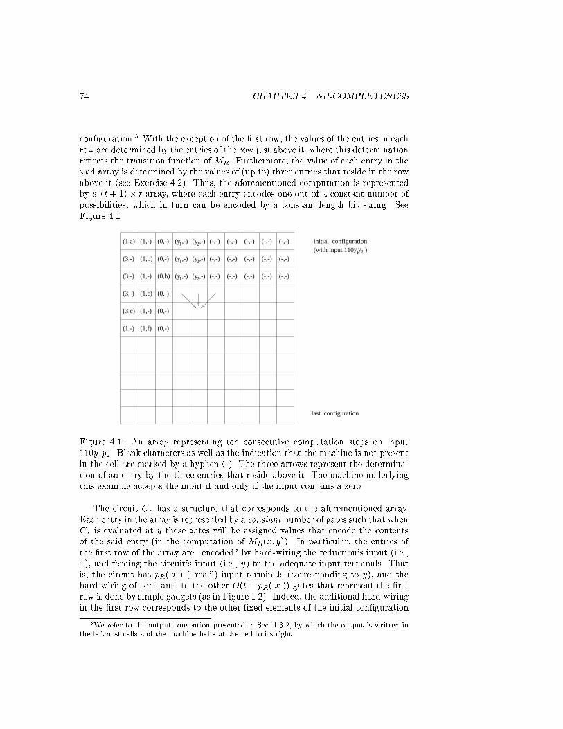
74 CHAPTER 4. NP-COMPLETENESScon�guration.5 With the exception of the �rst row, the values of the entries in eachrow are determined by the entries of the row just above it, where this determinationre ects the transition function of MR. Furthermore, the value of each entry in thesaid array is determined by the values of (up to) three entries that reside in the rowabove it (see Exercise 4.2). Thus, the aforementioned computation is representedby a (t + 1) � t array, where each entry encodes one out of a constant number ofpossibilities, which in turn can be encoded by a constant-length bit string. SeeFigure 4.1.

last configuration

initial configuration (1,a) (1,-) (0,-) (-,-) (-,-) (-,-)(-,-) (-,-)

(0,-) (-,-) (-,-) (-,-)(-,-) (-,-)

(-,-) (-,-) (-,-)(-,-) (-,-)

(1,b)

(0,b)(1,-)

(3,-)

(3,-)

(0,-)(1,c)(3,-)

(0,-)

(0,-)

(1,-)(3,c)

(y ,-)1

(y ,-)1

(y ,-)1 (y ,-)2

(y ,-)2

(y ,-)2

(with input 110 2 y 1 ) y

(1,-) (1,f)

Figure 4.1: An array representing ten consecutive computation steps on input110y1y2. Blank characters as well as the indication that the machine is not presentin the cell are marked by a hyphen (-). The three arrows represent the determina-tion of an entry by the three entries that reside above it. The machine underlyingthis example accepts the input if and only if the input contains a zero.The circuit Cx has a structure that corresponds to the aforementioned array.Each entry in the array is represented by a constant number of gates such that whenCx is evaluated at y these gates will be assigned values that encode the contentsof the said entry (in the computation of MR(x; y)). In particular, the entries ofthe �rst row of the array are \encoded" by hard-wiring the reduction's input (i.e.,x), and feeding the circuit's input (i.e., y) to the adequate input terminals. Thatis, the circuit has pR(jxj) (\real") input terminals (corresponding to y), and thehard-wiring of constants to the other O(t � pR(jxj)) gates that represent the �rstrow is done by simple gadgets (as in Figure 1.2). Indeed, the additional hard-wiringin the �rst row corresponds to the other �xed elements of the initial con�guration5We refer to the output convention presented in Sec. 1.3.2, by which the output is written inthe leftmost cells and the machine halts at the cell to its right.

4.3. SOME NATURAL NP-COMPLETE PROBLEMS 75(i.e., the blank symbols, and the encoding of the initial state and of the initiallocation; cf. Figure 4.1). The entries of subsequent rows will be \encoded" (orrather computed at evaluation time) by using constant-size circuits that determinethe value of an entry based on the three relevant entries in the row above it. Recallthat each entry is encoded by a constant number of gates, and thus these constant-size circuits merely compute the constant-size function described in Exercise 4.2.In addition, the circuit Cx has a few extra gates that check the values of theentries of the last row in order to determine whether or not it encodes an acceptingcon�guration.6 Note that the circuit Cx can be constructed in polynomial timefrom the string x, because we just need to encode x in an appropriate manner aswell as generate a \highly uniform" grid-like circuit of size O(tR(jxj+ pR(jxj))2).7Although the foregoing construction of Cx capitalizes on various speci�c detailsof the (one-tape) Turing machine model, it can be easily adapted to other naturalmodels of e�cient computation (by showing that in such models the transformationfrom one con�guration to the subsequent one can be emulated by a (polynomial-time constructible) circuit).8 Alternatively, we recall the Cobham-Edmonds Thesisasserting that any problem that is solvable in polynomial-time (on some \reason-able" model) can be solved in polynomial-time by a (one-tape) Turing machine.Turning back to the circuit Cx, we observe that indeed Cx(y) = 1 if and onlyif MR accepts the input (x; y) while making at most t = tR(jxj + pR(jxj)) steps.Recalling that S = fx : 9y s.t. jyj � pR(jxj) ^ (x; y) 2 Rg and that MR decidesmembership in R in time tR, we infer that x 2 S if and only if f(x) = Cx 2 CSAT.Furthermore, (x; y) 2 R if and only if (f(x); y) 2 RCSAT. It follows that f is aKarp-reduction of S to CSAT, and, for g(x; y) def= y, it holds that (f; g) is a Levin-reduction of R to RCSAT. The theorem follows.4.3.1.2 The NP-Completeness of SATRecall that Boolean formulae are special types of Boolean circuits (i.e., circuitshaving a tree structure).9 We further restrict our attention to formulae given inconjunctive normal form (CNF). We denote by SAT the set of satis�able CNFformulae (i.e., a CNF formula � is in SAT if there exists an truth assignment � suchthat �(�) = 1). We also consider the related relation RSAT = f(�; �) : �(�) = 1g.Theorem 4.6 (NP-completeness of SAT): The set (resp., relation) SAT (resp.,RSAT) is NP-complete (resp., PC-complete).6In continuation of Footnote 5, we note that it su�ces to check the values of the two leftmostentries of the last row. We assumed here that the circuit propagates a halting con�guration tothe last row. Alternatively, we may check for the existence of an accepting/halting con�gurationin the entire array, since this condition is quite simple.7Advanced comment: A more e�cient construction, which generate almost-linear sizedcircuits (i.e., circuits of size eO(tR(jxj+ pR(jxj)))) is known; see [24].8Advanced comment: Indeed, presenting such circuits is very easy in the case of all naturalmodels (e.g., the RAM model), where each bit in the next con�guration can be expressed by asimple Boolean formula in the bits of the previous con�guration.9For an alternative de�nition, see Section A.2.

76 CHAPTER 4. NP-COMPLETENESSProof: Since the set of possible instances of SAT is a subset of the set of instancesof CSAT, it is clear that SAT 2 NP (resp., RSAT 2 PC). To prove that SAT is NP-hard, we reduce CSAT to SAT (and use Proposition 4.4). The reduction boils downto introducing auxiliary variables in order to \cut" the computation of an arbitrary(\deep") circuit into a conjunction of related computations of \shallow" circuits(i.e., depth-2 circuits) of unbounded fan-in, which in turn may be presented as aCNF formula. The aforementioned auxiliary variables hold the possible values ofthe internal gates of the original circuit, and the clauses of the CNF formula enforcethe consistency of these values with the corresponding gate operation. For example,if gatei and gatej feed into gatek, which is a ^-gate, then the correspondingauxiliary variables gi; gj ; gk should satisfy the Boolean condition gk � (gi ^ gj),which can be written as a 3CNF with four clauses. Details follow.1 2 3

or

and

and

1 2

g1

3

g2g1 g2

and

g3

eq

or

eqeq

g4

eq

gate1

gate2

gate3and

3

gate4 neg

neg

g3 g4and

Figure 4.2: Using auxiliary variables (i.e., the gi's) to \cut" a depth-5 circuit (intoa CNF). The dashed regions will be replaced by equivalent CNF formulae. Thedashed cycle representing an unbounded fan-in and-gate is the conjunction of allconstant-size circuits (which enforce the functionalities of the original gates) andthe variable that represents the gate that feed the output terminal in the originalcircuit.We start by Karp-reducing CSAT to SAT. Given a Boolean circuit C, withn input terminals and m gates, we �rst construct m constant-size formulae onn +m variables, where the �rst n variables correspond to the input terminals ofthe circuit, and the other m variables correspond to its gates. The ith formula willdepend on the variable that correspond to the ith gate and the 1-2 variables thatcorrespond to the vertices that feed into this gate (i.e., 2 vertices in case of ^-gateor _-gate and a single vertex in case of a :-gate, where these vertices may be eitherinput terminals or other gates). This (constant-size) formula will be satis�ed bya truth assignment if and only if this assignment matches the gate's functionality(i.e., feeding this gate with the corresponding values result in the correspondingoutput value). Note that these constant-size formulae can be written as constant-size CNF formulae (in fact, as 3CNF formulae).10 Taking the conjunction of these10Recall that any Boolean function can be written as a CNF formula having size that is ex-ponential in the length of its input (cf. Exercise 1.12), which in this case is a constant (i.e.,

4.3. SOME NATURAL NP-COMPLETE PROBLEMS 77m formulae and the variable associated with the gate that feeds into the outputterminal, we obtain a formula � in CNF (see Figure 4.2, where n = 3 and m = 4).Note that � can be constructed in polynomial-time from the circuit C; that is,the mapping of C to � = f(C) is polynomial-time computable. We claim that Cis in CSAT if and only if � is in SAT.1. Suppose that for some string s it holds that C(s) = 1. Then, assigning tothe ith auxiliary variable the value that is assigned to the ith gate of C whenevaluated on s, we obtain (together with s) a truth assignment that satis�es�. This is the case because such an assignment satis�es all m constant-sizeCNFs as well as the variable associated with the output of C.2. On the other hand, if � satis�es � then the �rst n bits in � correspond to aninput on which C evaluates to 1. This is the case because the m constant-sizeCNFs guarantee that the variables of � are assigned values that correspondto the evaluation of C on the �rst n bits of � , while the fact that the variableassociated with the output of C has value true guarantees that this evaluationof C yields the value 1.Note that the latter mapping (of � to its n-bit pre�x) is the second mappingrequired by the de�nition of a Levin-reduction.Thus, we have established that f is a Karp-reduction of CSAT to SAT, and thataugmenting f with the aforementioned second mapping yields a Levin-reductionof RCSAT to RSAT.Comment. The fact that the second mapping required by the de�nition of aLevin-reduction is explicit in the proof of the validity of the corresponding Karp-reduction is a fairly common phenomenon. Actually (see Exercise 4.14), typical pre-sentations of Karp-reductions provide two auxiliary polynomial-time computablemappings (in addition to the main mapping of instances from one problem (e.g.,CSAT) to instances of another problem (e.g., SAT)): The �rst auxiliary mappingis of solutions for the preimage instance (e.g., of CSAT) to solutions for the imageinstance of the reduction (e.g., of SAT), whereas the second mapping goes the otherway around. For example, the proof of the validity of the Karp-reduction of CSAT toSAT, denoted f , speci�ed two additional mappings h and g such that (C; s) 2 RCSATimplies (f(C); h(C; s)) 2 RSAT and (f(C); �) 2 RSAT implies (C; g(C; �)) 2 RCSAT.Speci�cally, in the proof of Theorem 4.6, we used h(C; s) = (s; a1; :::; am) where aiis the value assigned to the ith gate in the evaluation of C(s), and g(C; �) beingthe n-bit pre�x of � . (Note that only the main mapping (i.e., f) and the secondauxiliary mapping (i.e., g) are required in the de�nition of a Levin-reduction.)3SAT. Note that the formulae resulting from the Karp-reduction presented inthe proof of Theorem 4.6 are in conjunctive normal form (CNF) with each clauseeither 2 or 3). Indeed, note that the Boolean functions that we refer to here depends on 2-3Boolean variables (since they indicate whether or not the corresponding values respect the gate'sfunctionality).

78 CHAPTER 4. NP-COMPLETENESSreferring to at most three variables. Thus, the foregoing reduction actually estab-lishes the NP-completeness of 3SAT (i.e., SAT restricted to CNF formula with upto three variables per clause). Alternatively, one may Karp-reduce SAT (i.e., satis-�ability of CNF formula) to 3SAT (i.e., satis�ability of 3CNF formula) by replacinglong clauses with conjunctions of three-variable clauses (using auxiliary variables;see Exercise 4.3). Either way, we get the following result, where the furthermorepart is proved by an additional reduction.Proposition 4.7 3SAT is NP-complete. Furthermore, the problem remains NP-complete also if we restrict the instances such that each variable appears in at mostthree clauses.Proof: The furthermore part is proved by a reduction from 3SAT. We just replaceeach occurrence of each Boolean variable by a new copy of this variable, and addclauses to enforce that all these copies are assigned the same value. Speci�cally, ifvariable z occurs t times in the original 3CNF formula �, then we introduce t newvariables (i.e., its \copies"), denoted z(1); :::; z(t), and replace the ith occurrence ofz in � by z(i). In addition, we add the clauses z(i+1)_:z(i) for i = 1:::; t (where t+1is understood as 1). Thus, each variable appears at most three times in the newformula. Note that the clause z(i+1) _:z(i) is logically equivalent to z(i) ) z(i+1),and thus the conjunction of the aforementioned t clauses is logically equivalent toz(1) , z(2) , � � � , z(t). The validity of the reduction follows.Related problems. Note that instances of SAT can be viewed as systems ofBoolean conditions over Boolean variables. Such systems can be emulated by vari-ous types of systems of arithmetic conditions, implying the NP-hardness of solvingthe latter types of systems. Examples include systems of integer linear inequalities(see Exercise 4.5), and systems of quadratic equalities (see Exercise 4.7).4.3.2 Combinatorics and Graph TheoryTeaching note: The purpose of this section is to expose the students to a sampleof NP-completeness results and proof techniques (i.e., the design of reductions amongcomputational problems).We present just a few of the many appealing combinatorial problems that are knownto be NP-complete. Throughout this section, we focus on the decision versions ofthe various problems, and adopt a more informal style. Speci�cally, we will presenta typical decision problem as a problem of deciding whether a given instance, whichbelongs to a set of relevant instances, is a \yes-instance" or a \no-instance" (ratherthan referring to deciding membership of arbitrary strings in a set of yes-instances).For further discussion of this style and its rigorous formulation, see Section 5.1. Wewill also neglect showing that these decision problems are in NP; indeed, for naturalproblems in NP, showing membership in NP is typically straightforward.

4.3. SOME NATURAL NP-COMPLETE PROBLEMS 79Set Cover. We start with the set cover problem, in which an instance consists ofa collection of �nite sets S1; :::; Sm and an integerK and the question (for decision)is whether or not there exist (at most)11 K sets that cover Smi=1 Si (i.e., indicesi1; :::; iK such that SKj=1 Sij = Smi=1 Si).Proposition 4.8 Set Cover is NP-complete.Proof Sketch: We sketch a reduction of SAT to Set Cover. For a CNF formula� with m clauses and n variables, we consider the sets S1;t; S1;f; ::; Sn;t; Sn;f �f1; :::;mg such that Si;t (resp., Si;f) is the set of the indices of the clauses (of �)that are satis�ed by setting the ith variable to true (resp., false). That is, if the ithvariable appears unnegated (resp., negated) in the jth clause then j 2 Si;t (resp.,j 2 Si;f). Indeed, Si;t [ Si;f equals the set of clauses containing an occurrence ofthe ith variable, and the union of all these 2n sets equals f1; :::;mg. Now, on input�, the reduction outputs the Set Cover instance f(�) def= ((S1; ::; S2n); n), whereS2i�1 = Si;t [ fm+ ig and S2i = Si;f [ fm+ ig for i = 1; :::; n.Note that f is computable in polynomial-time, and that if � is satis�ed by�1 � � � �n then the collection fS2i��i : i = 1; :::; ng covers f1; :::;m + ng (sincefS2i��i \ [m] : i = 1; :::; ng covers [m] and fS2i��i n [m] : i = 1; :::; ng coversfm + 1; :::;m + ng). Thus, � 2 SAT implies that f(�) is a yes-instance of SetCover. On the other hand, each cover of fm+ 1; :::;m+ ng � f1; :::;m+ ng mustinclude either S2i�1 or S2i for each i (since these are the only sets that cover theelement m+ i). Thus, a cover of f1; :::;m+ng using n of the Sj 's must contain, forevery i, either S2i�1 or S2i but not both. Setting �i accordingly (i.e., �i = 1 if andonly if S2i�1 is in the cover) implies that fS2i��i : i = 1; :::; ng covers f1; :::;mg,which in turn implies that �1 � � � �n satis�es �. Thus, if f(�) is a yes-instance ofSet Cover then � 2 SAT.Exact Cover and 3XC. The exact cover problem is similar to the set cover prob-lem, except that here the sets that are used in the cover are not allowed to intersect.That is, each element in the universe should be covered by exactly one set in thecover. Restricting the set of instances to sequences of sets each having exactly threeelements, we get the restricted problem called 3-Exact Cover (3XC), where it isunnecessary to specify the number of sets to be used in the cover. The problem 3XCis rather technical, but it is quite useful for demonstrating the NP-completeness ofother problems (by reducing 3XC to them); see, for example, Exercise 4.13.Proposition 4.9 3-Exact Cover is NP-complete.Indeed, it follows that the Exact Cover (in which sets of arbitrary size are allowed)is NP-complete. This follows both for the case that the number of sets in the desiredcover is unspeci�ed and for the various cases in which this number is bounded (i.e.,upper-bounded or lower-bounded or both).11Clearly, in case of Set Cover, the two formulations (i.e., asking for exactly K sets or at mostK sets) are computationally equivalent.

80 CHAPTER 4. NP-COMPLETENESSProof Sketch: The reduction is obtained by composing three reductions. We �rstreduce a restricted case of 3SAT to a restricted version of Set Cover, denoted 3SC,in which each set has at most three elements (and an instance consists, as in thegeneral case, of a sequence of �nite sets as well as an integer K). Speci�cally,we refer to 3SAT instances that are restricted such that each variable appears inat most three clauses, and recall that this restricted problem is NP-complete (seeProposition 4.7). Actually, we further reduce this restricted version of 3SAT to amore restricted version, denoted r3SAT, in which each literal appears in at mosttwo clauses (see Exercise 4.8). Now, we reduce r3SAT to 3SC by using the (verysame) reduction presented in the proof of Proposition 4.8, while observing that thesize of each set in the reduced instance is at most three (i.e., one more than thenumber of occurrences of the corresponding literal).Next, we reduce 3SC to the following restricted case of Exact Cover, denoted3XC0, in which each set has at most three elements, an instance consists of a sequenceof �nite sets as well as an integer K, and the question is whether there exists anexact cover with at most K sets. The reduction maps an instance ((S1; :::; Sm);K)of 3SC to the instance (C 0;K) such that C 0 is a collection of all subsets of each of thesets S1; :::; Sm. Since each Si has size at most 3, we introduce at most 7 non-emptysubsets per each such set, and the reduction can be computed in polynomial-time.The reader may easily verify the validity of this reduction (see Exercise 4.9).Finally, we reduce 3XC0 to 3XC. Consider an instance ((S1; :::; Sm);K) of 3XC0,and suppose that Smi=1 Si = [n]. If n > 3K then this is de�nitely a no-instance,which can be mapped to a dummy no-instance of 3XC, and so we assume thatx def= 3K � n � 0. Note that x represents the \excess" covering ability of anexact cover having K sets, each having three elements. Thus, we augment the setsystem with x new elements, denoted n+ 1; :::; 3K, and replace each Si such thatjSij < 3 by a sub-collection of 3-sets that cover Si as well as arbitrary elementsfrom fn + 1; :::; 3Kg. That is, in case jSij = 2, the set Si is replaced by the sub-collection (Si[fn+1g; :::; Si[f3Kg), whereas a singleton Si is replaced by the setsSi [ fj1; j2g for every j1 < j2 in fn + 1; :::; 3Kg. In addition, we add all possible3-subsets of fn+1; :::; 3Kg. This completes the description of the third reduction,the validity of which is left as an exercise (see Exercise 4.9).Vertex Cover, Independent Set, and Clique. Turning to graph theoreticproblems (see Section A.1), we start with the Vertex Cover problem, which isa special case of the Set Cover problem. The instances consists of pairs (G;K),where G = (V;E) is a simple graph andK is an integer, and the problem is whetheror not there exists a set of (at most) K vertices that is incident to all graph edges(i.e., each edge in G has at least one endpoint in this set). Indeed, this instanceof Vertex Cover can be viewed as an instance of Set Cover by considering thecollection of sets (Sv)v2V , where Sv denotes the set of edges incident at vertex v(i.e., Sv = fe 2 E : v 2 eg). Thus, the NP-hardness of Set Cover follows from theNP-hardness of Vertex Cover (but this implication is unhelpful for us here: wealready know that Set Cover is NP-hard and we wish to prove that Vertex Coveris NP-hard). We also note that the Vertex Cover problem is computationally

4.3. SOME NATURAL NP-COMPLETE PROBLEMS 81equivalent to the Independent Set and Clique problems (see Exercise 4.10), andthus it su�ces to establish the NP-hardness of one of these problems.Proposition 4.10 The problems Vertex Cover, Independent Set and Cliqueare NP-complete.Teaching note: The following reduction is not the \standard" one (see Exercise 4.11),but is rather adapted from the FGLSS-reduction (see [9]). This is done in anticipationof the use of the FGLSS-reduction in the context of the study of the complexity ofapproximation (cf., e.g., [14] or [13, Sec. 10.1.1]). Furthermore, although the followingreduction creates a larger graph, the author �nds it more clear than the \standard"reduction.Proof Sketch: We show a reduction from 3SAT to Independent Set. On inputa 3CNF formula � with m clauses and n variables, we construct a graph with 7mvertices, denoted G�. The vertices are grouped in m cliques, each correspondingto one of the clauses and containing 7 vertices that correspond to the 7 truth as-signments (to the 3 variables in the clause) that satisfy the clause. In addition tothe internal edges of these m cliques, we add an edge between each pair of verticesthat correspond to partial assignments that are mutually inconsistent. That is,if a speci�c (satisfying) assignment to the variables of the ith clause is inconsis-tent with some (satisfying) assignment to the variables of the jth clause, then weconnect the corresponding vertices by an edge. In particular, no edges are placedbetween cliques that represent clauses that share no common variable. (Note thatthe internal edges of the m cliques may be viewed as a special case of the edgesconnecting mutually inconsistent partial assignments.) To summarize, on input �,the reduction outputs the pair (G�;m), where G� is the aforementioned graph andm is the number of clauses in �.We stress that each clique of the graphG� contains only vertices that correspondto partial assignments that satisfy the corresponding clause; that is, the singlepartial assignments that does not satisfy this clause is not represented as a vertex inG�. Recall that the edges placed among vertices represent partial assignments thatare not mutually consistent. Thus, valid truth assignments to the entire formula� correspond to independent sets in G�, and the size of the latter represents thenumber of clauses that are satis�ed by the assignment. These observations underliethe validity of the reduction, which is argued next.Note that if � is satis�able by a truth assignment � , then there are no edgesbetween the m vertices that correspond to the partial satisfying assignments (forindividual clauses) derived from � . This assertion holds because any truth assign-ment � to � yields an independent set that contains a single vertex from each cliquethat corresponds to a clause that is satis�ed by � such that this vertex correspondsto the partial assignment (to this clause's variables) derived from � . Thus, if � is asatisfying assignment, then the aforementioned independent set contains a vertexfrom each of the m cliques. It follows that � 2 SAT implies that G� has an inde-pendent set of size m. On the other hand, any independent set of size m in G�must contain exactly one vertex in each of the m cliques, and thus induces a truth

82 CHAPTER 4. NP-COMPLETENESSassignment that satis�es �. This assertion follows by combining the following twofacts:1. Each independent set in G� induces a (consistent) truth assignment to �,because the partial assignments \selected" in the various cliques must beconsistent.2. Any independent set that contains a vertex from a speci�c clique induces atruth assignment that satis�es the corresponding clause.Thus, if G� has an independent set of size m then � 2 SAT.Graph 3-Colorability (G3C). In this problem the instances are graphs and thequestion is whether or not the graph can be colored using three colors such thatneighboring vertices are not assigned the same color.Proposition 4.11 Graph 3-Colorability is NP-complete.Proof Sketch: We reduce 3SAT to G3C by mapping a 3CNF formula � to the graphG� that consists of two special (\designated") vertices, a gadget per each variableof �, a gadget per each clause of �, and edges connecting some of these componentsas follows.� The two designated vertices are called ground and false, and are connectedby an edge that ensures that they must be given di�erent colors in any 3-coloring of G�. We will refer to the color assigned to the vertex ground (resp.,false) by the name ground (resp., false). The third color will be calledtrue.� The gadget associated with variable x is a pair of vertices, associated withthe two literals of x (i.e., x and :x). These vertices are connected by anedge, and each of them is also connected to the vertex ground. Thus, in any3-coloring of G� one of the vertices associated with the variable is coloredtrue and the other is colored false.1

2

3

x

yM

T1

T2

T3Figure 4.3: The clause gadget and its sub-gadget. In a generic 3-coloring of thesub-gadget it must hold that if x = y then x = y = 1. Thus, if the three terminalsof the gadget are assigned the same color, �, then M is also assigned the color �.

4.3. SOME NATURAL NP-COMPLETE PROBLEMS 83� The gadget associated with a clause C is depicted in Figure 4.3. It contains amaster vertex, denoted M, and three terminal vertices, denoted T1, T2 andT3. The master vertex is connected by edges to the vertices ground andfalse, and thus in any 3-coloring of G� the master vertex must be coloredtrue. The gadget has the property that it is possible to color the terminalswith any combination of the colors true and false, except for coloring allterminals with false. That is, in any 3-coloring of G�, if no terminal of aclause-gadget is colored ground, then at least one of these terminals is coloredtrue.The terminals of the gadget associated with clause C will be identi�ed withthe vertices (of variable-gadgets) that are associated with the correspondingliterals appearing in C. This means that each clause-gadget shares its ter-minals with the corresponding variable-gadgets, and that the various clause-gadgets are not vertex-disjoint but may rather share some terminals (i.e.,those associated with literals that appear in several clauses).12 See Figure 4.4.The aforementioned association forces each terminal to be colored either trueor false (in any 3-coloring of G�). By the foregoing discussion it follows that,in any 3-coloring of G�, at least one terminal of each clause-gadget must becolored true.variable gadgets

clause gadgets

GROUND FALSEthe two designated verices

Figure 4.4: A single clause gadget and the relevant variables gadgets.Verifying the validity of the reduction is left as an exercise (see Exercise 4.12).Digest. The reductions presented in the current section are depicted in Fig-ure 4.5, where bold arrows indicate reductions presented explicitly in the proofs of12Alternatively, we may use disjoint gadgets and \connect" each terminal with the correspond-ing literal (in the corresponding vertex gadget). Such a connection (i.e., an auxiliary gadget)should force the two end-points to have the same color in any 3-coloring of the graph.

84 CHAPTER 4. NP-COMPLETENESSthe various propositions (indicated by their index). Note that r3SAT and 3SC areonly mentioned inside the proof of Proposition 4.9.SAT 3SAT SC

r3SAT 3SC 3XC

IS

VC

Clique

G3C

4.7 4.8

(4.9)

(4.9) (4.9)

4.10

4.11

4.6CSAT

Figure 4.5: The (non-generic) reductions presented in Section 4.34.4 NP sets that are Neither in P nor NP-CompleteAs stated in Section 4.3, thousands of problems have been shown to be NP-complete(cf., [11, Apdx.], which contains a list of more than three hundreds main entries).Things reached a situation in which people seem to expect any NP-set to be eitherNP-complete or in P . This naive view is wrong: Assuming NP 6= P, there existsets in NP that are neither NP-complete nor in P, where here NP-hardness allowsalso Cook-reductions.Theorem 4.12 Assuming NP 6= P, there exist a set T in NP nP such that somesets in NP are not Cook-reducible to T .Theorem 4.12 asserts that if NP 6= P then NP is partitioned into three non-emptyclasses: the class P , the class of problems to which NP is Cook-reducible, and therest, denote NPI. We already know that the �rst two classes are not empty,and Theorem 4.12 establishes the non-emptiness of NPI under the condition thatNP 6= P , which is actually a necessary condition (because if NP = P then everyset in NP is Cook-reducible to any other set in NP).The following proof of Theorem 4.12 presents an unnatural decision problemin NPI. We mention that some natural decision problems (e.g., some that arecomputationally equivalent to factoring) are conjectured to be in NPI. We alsomention that if NP 6= coNP , where coNP = ff0; 1g� n S : S 2 NPg, then� def= NP \ coNP � P [ NPI holds (as a corollary to Theorem 5.7). Thus, ifNP 6= coNP then � n P is a (natural) subset of NPI, and the non-emptinessof NPI follows provided that � 6= P . Recall that Theorem 4.12 establishes thenon-emptiness of NPI under the seemingly weaker assumption that NP 6= P .

4.4. NP SETS THAT ARE NEITHER IN P NOR NP-COMPLETE 85Teaching note: We recommend either stating Theorem 4.12 without a proof or merelypresenting the proof idea.Proof Sketch: The basic idea is modifying an arbitrary set in NP n P so as tofail all possible reductions (from NP to the modi�ed set) as well as all possiblepolynomial-time decision procedures (for the modi�ed set). Speci�cally, startingwith S 2 NP nP , we derive S0 � S such that on one hand there is no polynomial-time reduction of S to S0 while on the other hand S0 2 NP n P . The process ofmodifying S into S0 proceeds in iterations, alternatively failing a potential reduction(by dropping su�ciently many strings from the rest of S) and failing a potentialdecision procedure (by including su�ciently many strings from the rest of S).Speci�cally, each potential reduction of S to S0 can be failed by dropping �nitelymany elements from the current S0, whereas each potential decision procedure canbe failed by keeping �nitely many elements of the current S0. These two assertionsare based on the following two corresponding facts:1. Any polynomial-time reduction (of any set not in P) to any �nite set (e.g.,a �nite subset of S) must fail, because only sets in P are Cook-reducible toa �nite set. Thus, for any �nite set F1 and any potential reduction (i.e.,a polynomial-time oracle machine), there exists an input x on which thisreduction to F1 fails.We stress that the aforementioned reduction fails while the only queries thatare answered positively are those residing in F1. Furthermore, the aforemen-tioned failure is due to a �nite set of queries (i.e., the set of all queries madeby the reduction when invoked on an input that is smaller or equal to x).Thus, for every �nite set F1 � S0 � S, any reduction of S to S0 can befailed by dropping a �nite number of elements from S0 and without droppingelements of F1.2. For every �nite set F2, any polynomial-time decision procedure for S n F2must fail, because S is Cook-reducible to S n F2. Thus, for any potentialdecision procedure (i.e., a polynomial-time algorithm), there exists an inputx on which this procedure fails.We stress that this failure is due to a �nite \pre�x" of S n F2 (i.e., the setfz 2 S n F2 : z � xg). Thus, for every �nite set F2, any polynomial-timedecision procedure for S nF2 can be failed by keeping a �nite subset of S nF2.As stated, the process of modifying S into S0 proceeds in iterations, alternativelyfailing a potential reduction (by dropping �nitely many strings from the rest of S)and failing a potential decision procedure (by including �nitely many strings fromthe rest of S). This can be done e�ciently because it is inessential to determine the�rst possible points of alternation (in which su�ciently many strings were dropped(resp., included) to fail the next potential reduction (resp., decision procedure)). Itsu�ces to guarantee that adequate points of alternation (albeit highly non-optimalones) can be e�ciently determined. Thus, S0 is the intersection of S and some setin P , which implies that S0 2 NP . Following are some comments regarding theimplementation of the foregoing idea.

86 CHAPTER 4. NP-COMPLETENESSThe �rst issue is that the foregoing plan calls for an (\e�ective") enumeration ofall polynomial-time oracle machines (resp., polynomial-time algorithms). However,none of these sets can be enumerated (by an algorithm). Instead, we enumerateall corresponding machines along with all possible polynomials, and for each pair(M;p) we consider executions of machine M with time bound speci�ed by thepolynomial p. That is, we use the machine Mp obtained from the pair (M;p) bysuspending the execution of M on input x after p(jxj) steps. We stress that we donot know whether machine M runs in polynomial-time, but the computations ofany polynomial-time machine is \covered" by some pair (M;p).Next, let us clarify the process in which reductions and decision procedures areruled out. We present a construction of a \�lter" set F in P such that the �nal setS0 will equal S \ F . Recall that we need to select F such that each polynomial-time reduction of S to S\F fails, and each polynomial-time procedure for decidingS \ F fails. The key observation is that for every �nite F 0 each polynomial-timereduction of S to (S \ F ) \ F 0 fails, whereas for every �nite F 0 each polynomial-time procedure for deciding (S \ F ) n F 0 fails. Furthermore, each of these failuresoccur on some input, and such an input can be determined by �nite portions ofS and F . Thus, we alternate between failing possible reductions and decisionprocedures on some inputs, while not trying to determine the \optimal" pointsof alternation but rather determining points of alternation in an e�cient manner(which in turn allows for e�ciently deciding membership in F ). Speci�cally, welet F = fx : f(jxj) � 1 mod 2g, where f : N ! f0g [ N will be de�ned such that(i) each of the �rst f(n)� 1 machines is failed by some input of length at most n,and (ii) the value f(n) can be computed in poly(n)-time.The value of f(n) is de�ned by the following process that performs exactlyn3 computation steps (where cubic-time is a rather arbitrary choice). The processproceeds in (an a priori unknown number of) iterations, where in the i+1st iterationwe try to �nd an input on which the i+ 1st (modi�ed) machine fails. Speci�cally,in the i + 1st iteration we scan all inputs, in lexicographic order, until we �nd aninput on which the i+1st (modi�ed) machine fails, where this machine is an oraclemachine if i+1 is odd and a standard machine otherwise. If we detect a failure ofthe i+ 1st machine, then we increment i and proceed to the next iteration. Whenwe reach the allowed number of steps (i.e., n3 steps), we halt outputting the currentvalue of i (i.e., the current i is output as the value of f(n)). Needless to say, thisdescription is heavily based on determining whether or not the i+1st machine failson speci�c inputs. Intuitively, these inputs will be much shorter than n, and soperforming these decisions in time n3 (or so) is not out of the question { see nextparagraph.In order to determine whether or not a failure (of the i + 1st machine) occurson a particular input x, we need to emulate the computation of this machine oninput x as well as determine whether x is in the relevant set (which is either S orS0 = S \ F ). Recall that if i+ 1 is even then we need to fail a standard machine(which attempts to decide S0) and otherwise we need to fail an oracle machine(which attempts to reduce S to S0). Thus, for even i + 1 we need to determinewhether x is in S0 = S \ F , whereas for odd i + 1 we need to determine whether

4.5. REFLECTIONS ON COMPLETE PROBLEMS 87x is in S as well as whether some other strings (which appear as queries) are inS0. Deciding membership in S 2 NP can be done in exponential-time (by usingthe exhaustive search algorithm that tries all possible NP-witnesses). Indeed, thismeans that when computing f(n) we may only complete the treatment of inputsthat are of logarithmic (in n) length, but anyhow in n3 steps we can not hope toreach (in our lexicographic scanning) strings of length greater than 3 log2 n. As fordeciding membership in F , this requires ability to compute f on adequate integers.That is, we may need to compute the value of f(n0) for various integers n0, but asnoted n0 will be much smaller than n (since n0 � poly(jxj) � poly(logn)). Thus,the value of f(n0) is just computed recursively (while counting the recursive stepsin our total number of steps).13 The point is that, when considering an input x,we may need the values of f only on f1; :::; pi+1(jxj)g, where pi+1 is the polynomialbounding the running-time of the i + 1st (modi�ed) machine, and obtaining sucha value takes at most pi+1(jxj)3 steps. We conclude that the number of stepsperformed towards determining whether or not a failure (of the i + 1st machine)occurs on the input x is upper-bounded by an (exponential) function of jxj.As hinted in the foregoing paragraph, the procedure will complete n3 stepsmuch before examining inputs of length greater than 3 log2 n, but this does notmatter. What matters is that f is unbounded (see Exercise 4.18). Furthermore,by construction, f(n) is computed in poly(n) time.Comment: The proof of Theorem 4.12 actually establishes that for every S 62 Pthere exists S0 62 P such that S0 is Karp-reducible to S but S is not Cook-reducibleto S0.14 Thus, if P 6= NP then there exists an in�nite sequence of sets S1; S2; :::in NP n P such that Si+1 is Karp-reducible to Si but Si is not Cook-reducibleto Si+1. That is, there exists an in�nite hierarchy of problems (albeit unnaturalones), all in NP , such that each problem is \easier" than the previous ones (in thesense that it can be reduced to the previous problems while these problems cannotbe reduced to it).4.5 Re ections on Complete ProblemsThis book will perhaps only be understood by those who havethemselves already thought the thoughts which are expressed init { or similar thoughts. It is therefore not a text-book. Its objectwould be attained if it a�orded pleasure to one who read it withunderstanding.Ludwig Wittgenstein, Tractatus Logico-PhilosophicusIndeed, this section should be viewed as an invitation to meditate together onquestions of the type what enables the existence of complete problems? Accordingly,13We do not bother to present a more e�cient implementation of this process. That is, we maya�ord to recompute f(n0) every time we need it (rather than store it for later use).14The said Karp-reduction (of S0 to S) maps x to itself if x 2 F and otherwise maps x to a�xed no-instance of S.

88 CHAPTER 4. NP-COMPLETENESSthe style is intentionally naive and imprecise; this entire section may be viewed asan open-ended exercise, asking the reader to consider substantiations of the vaguetext.Teaching note: This section/exercise may be unsuitable for most undergraduate stu-dents. We de�nitely do not intend it for presentation in class.We know that NP-complete problems exist. The question we ask here is whataspects in our modeling of problems enables the existence of complete problems.We should, of course, bear in mind that completeness refers to a class of problems;the complete problem should \encode" each problem in the class and be itself inthe class. Since the �rst aspect, hereafter referred to as encodability of a class, isamazing enough (at least to a layman), we start by asking what enables it. Weidentify two fundamental paradigms, regarding the modeling of problems, thatseem essential to the encodability of any (in�nite) class of problems:1. Each problem refer to an in�nite set of possible instances.2. The speci�cation of each problem uses a �nite description (e.g., an algorithmthat enumerates all the possible solutions for any given instance).15These two paradigms seem somewhat con icting, yet put together they suggest thede�nition of a universal problem. Speci�cally, this problem refers to instances ofthe form (D; x), where D is a description of a problem and x is an instance to thatproblem, and a solution to the instance (D; x) is a solution to x with respect tothe problem (described by) D. Intuitively, this universal problem can encode anyother problem (provided that problems are modeled in a way that conforms withthe foregoing paradigms): solving the universal problem allows solving any otherproblem.16Note that the foregoing universal problem is actually complete with respectto the class of all problems, but it is not complete with respect to any class thatcontains only (algorithmically) solvable problems (because this universal problemis not solvable). Turning our attention to classes of solvable problems, we seek ver-sions of the universal problem that are complete for these classes. One archetypicaldi�culty that arises is that, given a description D (as part of the instance to theuniversal problem), we cannot tell whether or not D is a description of a problemin a predetermined class C (because this decision problem is unsolvable). This factis relevant because17 if the universal problem requires solving instances that referto a problem not in C then intuitively it cannot be itself in C.15This seems the most naive notion of a description of a problem. An alternative notion ofa description refers to an algorithm that recognizes all valid instance-solution pairs (as in thede�nition of NP). However, at this point, we allow also \non-e�ective" descriptions (as giving riseto the Halting Problem).16Recall, however, that the universal problem is not (algorithmically) solvable. Thus, bothparts of the implication are false (i.e., this problem is not solvable and, needless to say, thereexists unsolvable problems). Indeed, the notion of a problem is rather vague at this stage; itcertainly extends beyond the set of all solvable problems.17Here we ignore the possibility of using promise problems, which do enable avoiding suchinstances without requiring anybody to recognize them. Indeed, using promise problems resolvesthis di�culty, but the issues discussed following the next paragraph remain valid.

4.5. REFLECTIONS ON COMPLETE PROBLEMS 89Before turning to the resolution of the foregoing di�culty, we note that theaforementioned modeling paradigms are pivotal to the theory of computation atlarge. In particular, so far we made no reference to any complexity consideration.Indeed, a complexity consideration is the key to resolving the foregoing di�culty:The idea is modifying any description D into a description D0 such that D0 isalways in C, and D0 agrees with D in the case that D is in C (i.e., in this casethey described exactly the same problem). We stress that in the case that D isnot in C, the corresponding problem D0 may be arbitrary (as long as it is in C).Such a modi�cation is possible with respect to many complexity theoretic classes.We consider two di�erent types of classes, where in both cases the class is de�nedin terms of the time-complexity of algorithms that do something related to theproblem (e.g., recognize valid solutions, as in the de�nition of NP).1. Classes de�ned by a single time-bound function t (e.g., t(n) = n3). In thiscase, any algorithm D is modi�ed to the algorithm D0 that, on input x,emulates (up to) t(jxj) steps of the execution of D(x). The modi�ed versionof the universal problem treats the instance (D; x) as (D0; x). This versioncan encode any problem in the said class C.But will this (version of the universal) problem be itself in C? The answerdepends both on the e�ciency of emulation in the corresponding computa-tional model and on the growth rate of t. For example, for triple-exponentialt, the answer will be de�nitely yes, because t(jxj) steps can be emulated inpoly(t(jxj)) time (in any reasonable model) while t(j(D; x)j) > t(jxj + 1) >poly(t(jxj)). On the other hand, in most reasonable models, the emulationof t(jxj) steps requires !(t(jxj)) time while for any polynomial t it holds thatt(n+O(1)) < 2t(n).2. Classes de�ned by a family of in�nitely many functions of di�erent growthrate (e.g., polynomials). We can, of course, select a function t that growsfaster than any function in the family and proceed as in the prior case, butthen the resulting universal problem will de�nitely not be in the class.Note that in the current case, a complete problem will indeed be striking be-cause, in particular, it will be associated with one function t0 that grows moremoderately than some other functions in the family (e.g., a �xed polynomialgrows more moderately than other polynomials). Seemingly this means thatthe algorithm describing the universal machine should be faster than somealgorithms that describe some other problems in the class. This impressionpresumes that the instances of both problems are (approximately) of the samelength, and so we intensionally violate this presumption by arti�cially increas-ing the length of the description of the instances to the universal problem. Forexample, if D is associated with the time bound tD, then the instance (D; x)to the universal problem is presented as, say, (D; x; 1t�10 (tD(jxj)2)), where inthe case of NP we used t0(n) = n.We believe that the last item explains the existence of NP-complete problems. Butwhat about the NP-completeness of SAT?

90 CHAPTER 4. NP-COMPLETENESSWe �rst note that the NP-hardness of CSAT is an immediate consequence ofthe fact that Boolean circuits can emulate algorithms.18 This fundamental fact isrooted in the notion of an algorithm (which postulates the simplicity of a singlecomputational step) and holds for any reasonable model of computation. Thus, forevery D and x, the problem of �nding a string y such that D(x; y) = 1 is \encoded"as �nding a string y such that CD;x(y) = 1, where CD;x is a Boolean circuit thatis easily derived from (D; x). In contrast to the fundamental fact underlying theNP-hardness of CSAT, the NP-hardness of SAT relies on a clever trick that allowsto encode instances of CSAT as instances of SAT.As stated, the NP-completeness of SAT is proved by encoding instances ofCSAT as instances of SAT. Similarly, the NP-completeness of other new problemsis proved by encoding instances of problems that are already known to be NP-complete. Typically, these encodings operate in a local manner, mapping smallcomponents of the original instance to local gadgets in the produced instance.Indeed, these problem-speci�c gadgets are the core of the encoding phenomenon.Presented with such a gadget, it is typically easy to verify that it works. Thus,one cannot be surprised by most of these gadgets, but the fact that they exist forthousands of natural problem is de�nitely amazing.ExercisesExercise 4.1 Prove that Bounded Halting and Bounded Non-Halting are NP-complete, where the problems are de�ned as follows. The instance consists of a pair(M; 1t), where M is a Turing machine and t is an integer. The decision version ofBounded Halting (resp., Bounded Non-Halting) consists of determining whetheror not there exists an input (of length at most t) on whichM halts (resp., does nothalt) in t steps, whereas the search problem consists of �nding such an input.Guideline: Either modify the proof of Theorem 4.3 or present a reduction of (say) thesearch problem of Ru to the search problem of Bounded (Non-)Halting. (Indeed, theexercise is more straightforward in the case of Bounded Halting.)Exercise 4.2 In the proof of Theorem 4.5, we claimed that the value of each entryin the \array of con�gurations" of a machine M is determined by the values of thethree entries that reside in the row above it (as in Figure 4.1). Present a functionfM : �3 ! �, where � = �� (Q [ f?g), that substantiates this claim.Guideline: For example, for every �1; �2; �3 2 �, it holds that fM((�1;?); (�2;?); (�3;?)) =(�2;?). More interestingly, if the transition function of M maps (�; q) to (�; p;+1)then, for every �1; �2; �3 2 Q, it holds that fM ((�; q); (�2;?); (�3;?)) = (�2; p) andfM ((�1;?); (�; q); (�3;?)) = (�;?).Exercise 4.3 Present and analyze a reduction of SAT to 3SAT.18The fact that CSAT is in NP is a consequence of the fact that the circuit evaluation problemis solvable in polynomial-time.

4.5. REFLECTIONS ON COMPLETE PROBLEMS 91Guideline: For a clause C, consider auxiliary variables such that the ith variable indicateswhether one of the �rst i literals is satis�ed, and replace C by a 3CNF that uses theoriginal variables of C as well as the auxiliary variables. For example, the clause _ti=1xiis replaced by the conjunction of 3CNFs that are logically equivalent to the formulae(y2 � (x1 _ x2)), (yi � (yi�1 _ xi)) for i = 3; :::; t, and yt. We comment that this isnot the standard reduction, but we �nd it conceptually more appealing. (The standardreduction replaces the clause _ti=1xi by the conjunction of the 3CNFs (x1 _ x2 _ z2),((:zi�1) _ xi _ zi) for i = 3; :::; t, and :zt.)Exercise 4.4 (e�cient solvability of 2SAT) In contrast to the NP-completenessof 3SAT, prove that 2SAT (i.e., the satis�ability of 2CNF formulae) is in P .Guideline: Consider the following forcing process for CNF formulae. If the formulacontains a singleton clause (i.e., a clause having a single literal), then the correspondingvariable is assigned the only value that satis�es the clause, and the formula is simpli�edaccordingly (possibly yielding a constant formula, which is either true or false). Theprocess is repeated until the formula is either a constant or contains only non-singletonclauses. Note that a formula � is satis�able if and only if the formula obtained from �by the forcing process is satis�able. Now, consider the following algorithm for solving thesearch problem associated with 2SAT.1. Choose an arbitrary variable in �. For each � 2 f0; 1g, denote by �� the formulaobtained from � by assigning this variable the value � and applying the forcingprocess to the resulting formula.Note that �� is either a Boolean constant or a 2CNF formula (which is a conjunctionof some clauses of �).2. If, for some � 2 f0; 1g, the formula �� equals the constant true, then we halt witha satisfying assignment for the original formula.3. If both assignments yield the constant false (i.e., for every � 2 f0; 1g the formula�� equals false), then we halt asserting that the original formula is unsatis�able.4. Otherwise (i.e.,, for each � 2 f0; 1g, the formula �� is a (non-constant) 2CNFformula), we select � 2 f0; 1g arbitrarily, set � ��, and goto Step 1.Proving the correctness of this algorithm boils down to observing that the arbitrary choicemade in Step 4 is immaterial. Indeed, this observation relies on the fact that we refer to2CNF formulae, which implies that the forcing process either yields a constant or a 2CNFformula (which is a conjunction of some clauses of the original �).Exercise 4.5 (Integer Linear Programming) Prove that the following prob-lem is NP-hard.19 An instance of the problem is a systems of linear inequalities(say with integer constants), and the problem is to determine whether the systemhas an integer solution. A typical instance of this decision problem follows.x+ 2y � z � 3�3x� z � �519Proving that the problem is in NP requires showing that if a system of linear inequalitieshas an integer solution, then it has an integer solution in which all numbers are of length that ispolynomial in the length of the description of the system. Such a proof is beyond the scope ofthe current textbook.

92 CHAPTER 4. NP-COMPLETENESSx � 0�x � �1Guideline: Reduce from SAT. Speci�cally, consider an arithmetization of the input CNFby replacing _ with addition and :x by 1�x. Thus, each clause gives rise to an inequality(e.g., the clause x _ :y is replaced by the inequality x + (1 � y) � 1, which simpli�esto x � y � 2). Enforce a 0-1 solution by introducing inequalities of the form x � 0 and�x � �1, for every variable x.Exercise 4.6 (Maximum Satis�ability of Linear Systems over GF(2)) Provethat the following problem is NP-complete. An instance of the problem consists ofa systems of linear equations over GF(2) and an integer k, and the problem is todetermine whether there exists an assignment that satis�es at least k equations.(Note that the problem of determining whether there exists an assignment thatsatis�es all the equations is in P .)Guideline: Reduce from 3SAT, using the following arithmetization. Replace each clausethat contains t � 3 literals by 2t � 1 linear GF(2) equations that correspond to thedi�erent non-empty subsets of these literals, and assert that their sum (modulo 2) equalsone; for example, the clause x_:y is replaced by the equations x+(1�y) = 1, x = 1, and1�y = 1. Identifying ffalse; trueg with f0; 1g, prove that if the original clause is satis�edby a Boolean assignment v then exactly 2t�1 of the corresponding equations are satis�edby v, whereas if the original clause is unsatis�ed by v then none of the correspondingequations is satis�ed by v.Exercise 4.7 (Satis�ability of Quadratic Systems over GF(2)) Prove that thefollowing problem is NP-complete. An instance of the problem consists of a systemof quadratic equations over GF(2), and the problem is to determine whether thereexists an assignment that satis�es all the equations. Note that the result holds alsofor systems of quadratic equations over the reals (by adding conditions that forcevalues in f0; 1g).Guideline: Start by showing that the corresponding problem for cubic equations is NP-complete, by a reduction from 3SAT that maps the clause x _ :y _ z to the equation(1 � x) � y � (1 � z) = 0. Reduce the problem for cubic equations to the problem forquadratic equations by introducing auxiliary variables; that is, given an instance withvariables x1; :::; xn, introduce the auxiliary variables xi;j 's and add equations of the formxi;j = xi � xj .Exercise 4.8 (restricted versions of 3SAT) Prove that the following restrictedversion of 3SAT, denoted r3SAT, is NP-complete. An instance of the problem con-sists of a 3CNF formula such that each literal appears in at most two clauses, andthe problem is to determine whether this formula is satis�able.Guideline: Recall that Proposition 4.7 establishes the NP-completeness of a version of3SAT in which the instances are restricted such that each variable appears in at most threeclauses. So it su�ces to reduce this restricted problem to r3SAT. This reduction is based

4.5. REFLECTIONS ON COMPLETE PROBLEMS 93on the fact that if all (three) occurrences of a variable are of the same type (i.e., they areall negated or all non-negated), then this variable can be assigned a value that satis�es allclauses in which it appears (and so the variable and the clauses in which it appear can beomitted from the instance). Thus, the desired reduction consists of applying the foregoingsimpli�cation to all relevant variables. Alternatively, a closer look at the reduction used inthe proof of Proposition 4.7 reveals the fact that this reduction maps any 3CNF formulato a 3CNF formula in which each literal appears in at most two clauses.Exercise 4.9 Verify the validity of the three reductions presented in the proof ofProposition 4.9; that is, we refer to the reduction of r3SAT to 3SC, the reductionof 3SC to 3XC0, and the reduction of 3XC0 to 3XC.Exercise 4.10 (Clique and Independent Set) An instance of the IndependentSet problem consists of a pair (G;K), where G is a graph and K is an integer,and the question is whether or not the graph G contains an independent set (i.e.,a set with no edges between its members) of size (at least) K. The Clique prob-lem is analogous. Prove that both problems are computationally equivalent viaKarp-reductions to the Vertex Cover problem.Exercise 4.11 (an alternative proof of Proposition 4.10) Consider the fol-lowing sketch of a reduction of 3SAT to Independent Set. On input a 3CNFformula � with m clauses and n variables, we construct a graph G� consisting of mtriangles (corresponding to the (three literals in the) m clauses) augmented withedges that link con icting literals. That is, if x appears as the ith1 literal of the jth1clause and :x appears as the ith2 literal of the jth2 clause, then we draw an edgebetween the ith1 vertex of the jth1 triangle and the ith2 vertex of the jth2 triangle.Prove that � 2 3SAT if and only if G� has an independent set of size m.Exercise 4.12 Verify the validity of the reduction presented in the proof of Propo-sition 4.11.Exercise 4.13 (Subset Sum) Prove that the following problem is NP-complete.The instance consists of a list of n+1 integers, denoted a1; :::; an; b, and the questionis whether or not a subsets of the ai's sums up to b (i.e., exists I � [n] such thatPi2I ai = b). Establish the NP-completeness of this problem, called subset sum,by reduction from 3XC.Guideline: Given an instance (S1; :::; Sm) of 3XC, where (without loss of generality)S1; :::; Sm � [3k], consider the following instance of subset sum that consists of a list ofm+ 1 integers such that b =P3kj=1(m+ 1)j and ai =Pj2Si(m+ 1)j for every i 2 [m].(Some intuition may be gained by writing all integers in base m+ 1.)Exercise 4.14 (additional properties of standard reductions) In continua-tion of the discussion in the main text, consider the following augmented form ofLevin-reductions. Such a reduction of R to R0 consists of three polynomial-timemappings (f; h; g) such that f is a Karp-reduction of SR to SR0 and the followingtwo conditions hold:1. For every (x; y) 2 R it holds that (f(x); h(x; y)) 2 R0.

94 CHAPTER 4. NP-COMPLETENESS2. For every (f(x); y0) 2 R0 it holds that (x; g(x; y0)) 2 R.(We note that this de�nition is actually the one used by Levin in [20], except thathe restricted h and g to only depend on their second argument.)Prove that such a reduction implies both a Karp-reduction and a Levin-Reduction,and show that all reductions presented in this chapter satisfy this augmented re-quirement. Furthermore, prove that in all these cases the main mapping (i.e., f)is 1-1 and polynomial-time invertible.Exercise 4.15 (parsimonious reductions) Let R;R0 2 PC and let f be a Karp-reduction of SR = fx : R(x) 6=;g to SR0 = fx : R0(x) 6=;g. We say that f is parsi-monious (with respect to R and R0) if for every x it holds that jR(x)j = jR0(f(x))j.For each of the reductions presented in this chapter, checked whether or not itis parsimonious. For the reductions that are not parsimonious, �nd alternativereductions that are parsimonious (cf. [11, Sec. 7.3]).Exercise 4.16 (on polynomial-time invertible reductions (following [2]))We say that a set S is markable if there exists a polynomial-time (marking) algo-rithm M such that1. For every x; � 2 f0; 1g� it holds that(a) M(x; �) 2 S if and only if x 2 S.(b) jM(x; �)j > jxj.2. There exists a polynomial-time (de-marking) algorithmD such that, for everyx; � 2 f0; 1g�, it holds that D(M(x; �)) = �.Note that all natural NP-sets (e.g., those considered in this chapter) are markable(e.g., for SAT, one may mark a formula by augmenting it with additional satis�-able clauses that use specially designated auxiliary variables). Prove that if S0 isKarp-reducible to S and S is markable then S0 is Karp-reducible to S by a length-increasing, one-to-one, and polynomial-time invertible mapping.20 Infer that forany natural NP-complete problem S, any set in NP is Karp-reducible to S by alength-increasing, one-to-one, and polynomial-time invertible mapping.Guideline: Let f be a Karp-reduction of S0 to S, and let M be the guaranteed markingalgorithm. Consider the reduction that maps x to M(f(x); x).Exercise 4.17 (on the isomorphism of NP-complete sets (following [2]))Suppose that S and T are Karp-reducible to one another by length-increasing, one-to-one, and polynomial-time invertible mappings, denoted f and g respectively.Using the following guidelines, prove that S and T are \e�ectively" isomorphic;that is, present a polynomial-time computable and invertible one-to-one mapping� such that T = �(S) def= f�(x) : x2Sg.20When given a string that is not in the image of the mapping, the inverting algorithm returnsa special symbol.

4.5. REFLECTIONS ON COMPLETE PROBLEMS 951. Let F def= ff(x) : x 2 f0; 1g�g and G def= fg(x) : x 2 f0; 1g�g. Using thelength-preserving condition of f (resp., g), prove that F (resp., G) is a propersubset of f0; 1g�. Prove that for every y 2 f0; 1g� there exists a unique triple(j; x; i) 2 f1; 2g � f0; 1g� � (f0g [ N) that satis�es one of the following twoconditions:(a) j = 1, x 2 G def= f0; 1g� nG, and y = (g � f)i(x);(b) j = 2, x 2 F def= f0; 1g� n F , and y = (g � f)i(g(x)).(In both cases h0(z) = z, hi(z) = h(hi�1(z)), and (g � f)(z) = g(f(z)). Hint:consider the maximal sequence of inverse operations g�1; f�1; g�1; ::: thatcan be applied to y, and note that each inverse shrinks the current string.)2. Let U1 def= f(g �f)i(x) : x2G^ i�0g and U2 def= f(g �f)i(g(x)) : x2F ^ i�0g.Prove that (U1; U2) is a partition of f0; 1g�. Using the fact that f and g arelength increasing and polynomial-time invertible, present a polynomial-timeprocedure for deciding membership in the set U1.Prove the same for the sets V1 = f(f � g)i(x) : x 2 F ^ i � 0g and V2 =f(f � g)i(f(x)) : x2G ^ i�0g.3. Note that U2 � G, and de�ne �(x) def= f(x) if x 2 U1 and �(x) def= g�1(x)otherwise.(a) Prove that � is a Karp-reduction of S to T .(b) Note that � maps U1 to f(U1) = ff(x) : x 2 U1g = V2 and U2 tog�1(U2) = fg�1(x) : x2U2g = V1. Prove that � is one-to-one and onto.Observe that ��1(x) = f�1(x) if x 2 f(U1) and ��1(x) = g(x) otherwise.Prove that ��1 is a Karp-reduction of T to S. Infer that �(S) = T .Using Exercise 4.16, infer that all natural NP-complete sets are isomorphic.Exercise 4.18 Referring to the proof of Theorem 4.12, prove that the function fis unbounded (i.e., for every i there exists an n such that n3 steps of the processde�ned in the proof allow for failing the i+ 1st machine).Guideline: Note that f is monotonically non-decreasing (because more steps allow to failat least as many machines). Assume, towards the contradiction that f is bounded. Leti = supn2Nff(n)g and n0 be the smallest integer such that f(n0) = i. If i is odd then theset F determined by f is co-�nite (because F = fx : f(jxj)�1 (mod 2)g � fx : jxj�n0g).In this case, the i+1st machine tries to decide S\F (which di�ers from S on �nitely manystrings), and must fail on some x. Derive a contradiction by showing that the number ofsteps taken till reaching and considering this x is at most exp(poly(jxj)), which is smallerthan n3 for some su�ciently large n. A similar argument applies to the case that i iseven, where we use the fact that F � fx : jxj<n0g is �nite and so the relevant reductionof S to S \ F must fail on some input x.

96 CHAPTER 4. NP-COMPLETENESS

Chapter 5Three relatively advancedtopicsIn this chapter we discuss three relatively advanced topics. The �rst topic, whichwas eluded to in previous chapters, is the notion of promise problems (Section 5.1).Next, we present an optimal algorithm for solving (\candid") NP search problems(Section 5.2). Finally, in Section 5.3, we brie y discuss the class (denoted coNP)of sets that are complements of sets in NP.Teaching note: The foregoing topics are typically not mentioned in a basic course oncomplexity. Still, pending on time constraints, we suggest discussing them at least at ahigh level.5.1 Promise ProblemsPromise problems are a natural generalization of search and decision problems,where one explicitly considers a set of legitimate instances (rather than consider-ing any string as a legitimate instance). As noted previously, this generalizationprovides a more adequate formulation of natural computational problems (and in-deed this formulation is used in all informal discussions). For example, in Sec. 4.3.2we presented such problems using phrases like \given a graph and an integer..." (or\given a collection of sets..."). In other words, we assumed that the input instancehas a certain format (or rather we \promised the solver" that this is the case).Indeed, we claimed that in these cases the assumption can be removed without af-fecting the complexity of the problem, but we avoided providing a formal treatmentof this issue, which is done next.Teaching note: The notion of promise problems was originally introduced in thecontext of decision problems, and is typically used only in that context. However, webelieve that promise problems are as natural in the context of search problems.97

98 CHAPTER 5. THREE RELATIVELY ADVANCED TOPICS5.1.1 De�nitionsPromise problems are de�ned by specifying a set of admissible instances. Candidatesolvers of these problems are only required to handle these admissible instances.Intuitively, the designer of an algorithm solving such a problem is promised thatthe algorithm will never encounter an inadmissible instance (and so the designerneed not care about how the algorithm performs on inadmissible inputs).5.1.1.1 Search problems with a promiseIn the context of search problems, a promise problem is a relaxation in which oneis only required to �nd solutions to instances in a predetermined set, called thepromise. The requirement regarding e�cient checkability of solutions is adapted inan analogous manner.De�nition 5.1 (search problems with a promise): A search problem with a promiseconsists of a binary relation R � f0; 1g� � f0; 1g� and a promise set P . Such aproblem is also referred to as the search problem R with promise P .� The search problem R with promise P is solved by algorithm A if for everyx 2 P it holds that (x;A(x)) 2 R if x 2 SR = fx : R(x) 6= ;g and A(x) = ?otherwise, where R(x) = fy : (x; y) 2 Rg.The time complexity of A on inputs in P is de�ned as TAjP (n) def= maxx2P\f0;1gnftA(x)g,where tA(x) is the running time of A(x) and TAjP (n) = 0 if P \ f0; 1gn = ;.� The search problem R with promise P is in the promise problem extension ofPF if there exists a polynomial-time algorithm that solves this problem.1� The search problem R with promise P is in the promise problem extension ofPC if there exists a polynomial T and an algorithm A such that, for everyx 2 P and y 2 f0; 1g�, algorithm A makes at most T (jxj) steps and it holdsthat A(x; y) = 1 if and only if (x; y) 2 R.We stress that nothing is required of the solver in the case that the input violatesthe promise (i.e., x 62 P ); in particular, in such a case the algorithm may halt witha wrong output. (Indeed, the standard formulations of PF and PC are obtainedby considering the trivial promise P = f0; 1g�.)2 In addition to the foregoingmotivation for promise problems, we mention one natural class of search problemswith a promise. These are search problem in which the promise is that the instancehas a solution (i.e., in terms of the foregoing notation P = SR, where SR def= fx :9y s.t. (x; y) 2 Rg). We refer to such search problems by the name candid searchproblems.1In this case it does not matter whether the time complexity of A is de�ned on inputs in Por on all possible strings. Suppose that A has (polynomial) time complexity T on inputs in P ,then we can modify A to halt on any input x after at most T (jxj) steps. This modi�cation mayonly e�ects the output of A on inputs not in P (which is OK by us). The modi�cation can beimplemented in polynomial-time by computing t = T (jxj) and emulating the execution of A(x)for t steps. A similar comment applies to the de�nition of PC, P and NP.2Here we refer to the formulation of PC outlined in Section 2.4.

5.1. PROMISE PROBLEMS 99De�nition 5.2 (candid search problems): An algorithm A solves the candid searchproblem of the binary relation R if for every x 2 SR (i.e., for every (x; y) 2 R) itholds that (x;A(x)) 2 R. The time complexity of such an algorithm is de�ned asTAjSR(n) def= maxx2P\f0;1gnftA(x)g, where tA(x) is the running time of A(x) andTAjSR(n) = 0 if SR \ f0; 1gn = ;.Note that nothing is required when x 62 SR: In particular, algorithm A may ei-ther output a wrong solution (although no solutions exist) or run for more thanTAjSR(jxj) steps. The �rst case can be essentially eliminated whenever R 2 PC.Furthermore, for R 2 PC, if we \know" the time complexity of algorithm A (e.g.,if we can compute TAjSR(n) in poly(n)-time), then we may modify A into an algo-rithm A0 that solves the (general) search problem of R (i.e., halts with a correctoutput on each input) in time TA0(n) = TAjSR(n) + poly(n). However, we do notnecessarily know the running-time of an algorithm that we consider. Furthermore,as we shall see in Section 5.2, the naive assumption by which we always know therunning-time of an algorithm that we design is not valid either.5.1.1.2 Decision problems with a promiseIn the context of decision problems, a promise problem is a relaxation in which oneis only required to determine the status of instances that belong to a predeterminedset, called the promise. The requirement of e�cient veri�cation is adapted in ananalogous manner. In view of the standard usage of the term, we refer to deci-sion problems with a promise by the name promise problems. Formally, promiseproblems refer to a three-way partition of the set of all strings into yes-instances,no-instances, and instances that violate the promise. Standard decision problemsare obtained as a special case by insisting that all inputs are allowed (i.e., thepromise is trivial).De�nition 5.3 (promise problems): A promise problem consists of a pair of non-intersecting sets of strings, denoted (Syes; Sno), and Syes[Sno is called the promise.� The promise problem (Syes; Sno) is solved by algorithm A if for every x 2 Syesit holds that A(x) = 1 and for every x 2 Sno it holds that A(x) = 0. Thepromise problem is in the promise problem extension of P if there exists apolynomial-time algorithm that solves it.� The promise problem (Syes; Sno) is in the promise problem extension of NP ifthere exists a polynomial p and a polynomial-time algorithm V such that thefollowing two conditions hold:1. Completeness: For every x 2 Syes, there exists y of length at most p(jxj)such that V (x; y) = 1.2. Soundness: For every x 2 Sno and every y, it holds that V (x; y) = 0.We stress that for algorithms of polynomial-time complexity, it does not matterwhether the time complexity is de�ned only on inputs that satisfy the promise oron all strings (see Footnote 1). Thus, the extended classes P and NP (like PFand PC) are invariant under this choice.

100 CHAPTER 5. THREE RELATIVELY ADVANCED TOPICS5.1.1.3 Reducibility among promise problemsThe notion of a Cook-reduction extend naturally to promise problems, when pos-tulating that a query that violates the promise (of the problem at the target of thereduction) may be answered arbitrarily.3 That is, the oracle machine should solvethe original problem no matter how queries that violate the promise are answered.The latter requirement is consistent with the conceptual meaning of reductions andpromise problems. Recall that reductions captures procedures that make subrou-tine calls to an arbitrary procedure that solves the reduced problem. But, in thecase of promise problems, such a solver may behave arbitrarily on instances thatviolate the promise. We stress that the main property of a reduction is preserved(see Exercise 5.1): if the promise problem � is Cook-reducible to a promise problemthat is solvable in polynomial-time, then � is solvable in polynomial-time.Caveat: The extension of a complexity class to promise problems does not nec-essarily inherit the \structural" properties of the standard class. For example, incontrast to Theorem 5.7, there exists promise problems in NP \ coNP such thatevery set in NP can be Cook-reduced to them: see Exercise 5.2. Needless to say,NP = coNP does not seem to follow from Exercise 5.2. See further discussion atthe end of Sec. 5.1.2.5.1.2 ApplicationsThe following discussion refers both to the decision and search versions of promiseproblems. Recall that promise problems o�er the most direct way of formulatingnatural computational problems. Indeed, this is a major application of the notionof promise problems (although this application usually goes unnoticed). Formally,the presentation of natural computational problems refers (usually implicitly) tosome natural format, and the notion of a promise problem allows us to discardinputs that do not adhere to this format (and focus on those that do adhere toit).4 For example, when referring to computational problems regarding graphs, thepromise mandates that the input is a graph (or rather a standard representationof some graph).Restricting a computational problem. In addition to the foregoing applica-tion of promise problems, we mention their use in formulating the natural notion ofa restriction of a computational problem to a subset of the instances. Speci�cally,such a restriction means that the promise set of the restricted problem is a subsetof the promise set of the unrestricted problem.De�nition 5.4 (restriction of computational problems):3It follows that Karp-reductions among promise problems are not allowed to make queriesthat violate the promise. Speci�cally, we say that the promise problem � = (�yes ;�no) is Karp-reducible to the promise problem �0 = (�0yes;�0no) if there exists a polynomial-time mapping fsuch that for every x 2 �yes (resp., x 2 �no) it holds that f(x) 2 �0yes (resp., f(x) 2 �0no).4This practice is supported by the fact that the said format is easily recognizable (seeSec. 5.1.3).

5.1. PROMISE PROBLEMS 101� For any P 0 � P and binary relation R, we say that the search problem Rwith promise P 0 is a restriction of the search problem R with promise P .� We say that the promise problem (S0yes; S0no) is a restriction of the promiseproblem (Syes; Sno) if both S0yes � Syes and S0no � Sno hold.For example, when we say that 3SAT is a restriction of SAT, we refer to the factthat the set of allowed instances is now restricted to 3CNF formulae (rather than toarbitrary CNF formulae). In both cases, the computational problem is to determinesatis�ability (or to �nd a satisfying assignment), but the set of instances (i.e., thepromise set) is further restricted in the case of 3SAT. The fact that a restrictedproblem is never harder than the original problem is captured by the fact that therestricted problem is Karp-reducible to the original one (via the identity mapping).Other uses and some reservations. In addition to the two aforementionedgeneric uses of the notion of a promise problem, we mention that this notionprovides adequate formulations for a variety of speci�c computational complex-ity notions and results. Examples include the notion of \unique solutions" (see [13,Sec. 6.2.3]) and the formulation of \gap problems" as capturing various approxi-mation tasks (see [13, Sec. 10.1]). In all these cases, promise problems allow todiscuss natural computational problems and make statements about their inherentcomplexity. Thus, the complexity of promise problems (and classes of such prob-lems) addresses natural questions and concerns. Consequently, demonstrating theintractability of a promise problem that belongs to some class (e.g., saying thatsome promise problem in NP cannot be solved by a polynomial-time algorithm)carries the same conceptual message as demonstrating the intractability of a stan-dard problem in the corresponding class. In contrast (as indicated in the caveatof Sec. 5.1.1.3), structural properties of promise problems may not hold for thecorresponding classes of standard problems (e.g., see Exercise 5.2). Indeed, we dodistinguish here between the inherent (or absolute) properties such as intractabilityand structural (or relative) properties such as reducibility.5.1.3 The Standard Convention of Avoiding Promise Prob-lemsRecall that, although promise problems provide a good framework for presentingnatural computational problems, we managed to avoid this framework in previouschapters. This was done by relying on the fact that, for all the (natural) problemsconsidered in the previous chapters, it is easy to decide whether or not a giveninstance satis�es the promise. For example, given a formula it is easy to decidewhether or not it is in CNF (or 3CNF). Actually, the issue arises already whentalking about formulae: What we are actually given is a string that is supposed toencode a formula (under some predetermined encoding scheme), and so the promise(which is easy to decide for natural encoding schemes) is that the input string is avalid encoding of some formula. In any case, if the promise is e�ciently recognizable

102 CHAPTER 5. THREE RELATIVELY ADVANCED TOPICS(i.e., membership in it can be decided in polynomial-time) then we may avoidmentioning the promise by using one of the following two \nasty" conventions:1. Fictitious extending the set of instances to the set of all possible strings (andallowing trivial solutions for the corresponding dummy instances). For ex-ample, in the case of a search problem, we may either de�ne all instancethat violate the promise to have no solution or de�ne them to have a trivialsolution (e.g., be a solution for themselves); that is, for a search problem Rwith promise P , we may consider the (standard) search problem of R whereR is modi�ed such that R(x) = ; for every x 62 P (or, say, R(x) = fxg forevery x 62 P ). In the case of a promise (decision) problem (Syes; Sno), wemay consider the problem of deciding membership in Syes, which means thatinstances that violate the promise are considered as no-instances.2. Considering every string as a valid encoding of some object that satis�es thepromise. That is, �xing any string x0 that satis�es the promise, we considerevery string that violates the promise as if it were x0. In the case of a searchproblem R with promise P , this means considering the (standard) searchproblem of R where R is modi�ed such that R(x) = R(x0) for every x 62 P .Similarly, in the case of a promise (decision) problem (Syes; Sno), we considerthe problem of deciding membership in Syes (provided x0 2 Sno and otherwisewe consider the problem of deciding membership in f0; 1g� n Sno).We stress that in the case that the promise is e�ciently recognizable the aforemen-tioned conventions (or modi�cations) do not e�ect the complexity of the relevant(search or decision) problem. That is, rather than considering the original promiseproblem, we consider a (search or decision) problem (without a promise) that iscomputational equivalent to the original one. Thus, in some sense we loss noth-ing by studying the latter problem rather than the original one (i.e., the originalpromise problem). However, to get to this situation we need the notion of a promiseproblem, which allows a formulation of the original natural problem.Indeed, even in the case that the original natural (promise) problem and theproblem (without a promise) that was derived from it are computationally equiv-alent, it is useful to have a formulation that allows to distinguish between them(as we do distinguish between the di�erent NP-complete problems although theyare all computationally equivalent). This conceptual concern becomes of crucialimportance in the case (to be discussed next) that the promise (referred to in thepromise problem) is not e�ciently recognizable.The point is that the foregoing transformations of promise problems into com-putationally equivalent standard (decision and search) problems do not necessar-ily preserve the complexity of the problem in the case that the promise is note�ciently recognizable. In this case, the terminology of promise problems is un-avoidable. Consider, for example, the problem of deciding whether a Hamiltoniangraph is 3-colorable. On the face of it, such a problem may have fundamentallydi�erent complexity than the problem of deciding whether a given graph is bothHamiltonian and 3-colorable.

5.2. OPTIMAL SEARCH ALGORITHMS FOR NP 103In spite of the foregoing issues, we adopt the convention of focusing on standarddecision and search problems. That is, by default, all computational problems andcomplexity classes discussed in other sections of this book refer to standard decisionand search problems, and the only exception in which we refer to promise problemsoutside the current section is explicitly stated as such (see Section 5.2).5.2 Optimal search algorithms for NPActually, this section refers to solving the candid search problem of any relation inPC. Recall that PC is the class of search problems that allow for e�cient checkingof the correctness of candidate solutions (see De�nition 2.3), and that the candidsearch problem is a search problem in which the solver is promised that the giveninstance has a solution (see De�nition 5.2).We claim the existence of an optimal algorithm for solving the candid searchproblem of any relation in PC. Furthermore, we will explicitly present such analgorithm, and prove that it is optimal in a very strong sense: for any algorithmsolving the candid search problem of R 2 PC, our algorithm solves the sameproblem in time that is at most a constant factor slower (ignoring a �xed additivepolynomial term, which may be disregarded in the case that the problem is notsolvable in polynomial-time). Needless to say, we do not know the time-complexityof the aforementioned optimal algorithm (indeed, if we knew it, then we wouldhave resolved the P-vs-NP Question). In fact, the P-vs-NP Question boils downto determining the time-complexity of a single explicitly presented algorithm (i.e.,the optimal algorithm claimed in Theorem 5.5).Theorem 5.5 For every binary relation R 2 PC there exists an algorithm A thatsatis�es the following:1. Algorithm A solves the candid search problem of R.2. There exists a polynomial p such that for every algorithm A0 that solves thecandid search problem of R, it holds that tA(x) = O(tA0(x) + p(jxj)) (for anyx 2 SR), where tA(x) (resp., tA0(x)) denotes the number of steps taken by A(resp., A0) on input x.Interestingly, we establish the optimality of A without knowing what its (optimal)running-time is. Furthermore, the optimality claim is \point-wise" (i.e., it refers toany input) rather than \global" (i.e., referring to the (worst-case) time-complexityas a function of the input length).We stress that the hidden constant in the O-notation depends only on A0,but in the following proof this dependence is exponential in the length of thedescription of algorithm A0 (and it is not known whether a better dependence canbe achieved). Indeed, this dependence as well as the idea underlying it constituteone negative aspect of this otherwise amazing result. Another negative aspect isthat the optimality of algorithm A refers only to inputs that have a solution (i.e.,inputs in SR). Finally, we note that the theorem as stated refers only to models of

104 CHAPTER 5. THREE RELATIVELY ADVANCED TOPICScomputation that have machines that can emulate a given number of steps of othermachines with a constant overhead. We mention that in most natural models theoverhead of such emulation is at most poly-logarithmic in the number of steps, inwhich case it holds that tA(x) = eO(tA0(x) + p(jxj)).Proof Sketch: Fixing R, we let M be a polynomial-time algorithm that decidesmembership in R, and let p be a polynomial bounding the running-time of M(as a function of the length of the �rst element in the input pair). Using M , wepresent an algorithm A that solves the candid search problem of R as follows. Oninput x, algorithm A emulates (\in parallel") the executions of all possible searchalgorithms (on input x), checks the result provided by each of them (using M),and halts whenever it recognizes a correct solution. Indeed, most of the emulatedalgorithms are totally irrelevant to the search, but using M we can screen the badsolutions o�ered by them, and output a good solution once obtained.Since there are in�nitely many possible algorithms, it may not be clear whatwe mean by the expression \emulating all possible algorithms in parallel." Whatwe mean is emulating them at di�erent \rates" such that the in�nite sum of theserates converges to 1 (or to any other constant). Speci�cally, we will emulate the ithpossible algorithm at rate 1=(i+ 1)2, which means emulating a single step of thisalgorithm per (i + 1)2 emulation steps (performed for all algorithms). Note thata straightforward implementation of this idea may create a signi�cant overhead,involved in switching frequently from the emulation of one machine to the emulationof another. Instead, we present an alternative implementation that proceeds initerations.In the jth iteration, for i = 1; :::; 2j=2�1, algorithm A emulates 2j=(i+1)2 stepsof the ith machine (where the machines are ordered according to the lexicographicorder of their descriptions). Each of these emulations is conducted in one chunk,and thus the overhead of switching between the various emulations is insigni�cant(in comparison to the total number of steps being emulated). In the case thatsome of these emulations (on input x) halts with output y, algorithm A invokesM on input (x; y), and output y if and only if M(x; y) = 1. Furthermore, theveri�cation of a solution provided by a candidate algorithm is also emulated at theexpense of its step-count. (Put in other words, we augment each algorithm witha canonical procedure (i.e., M) that checks the validity of the solution o�ered bythe algorithm.)By its construction, whenever A(x) outputs a string y (i.e., y 6= ?) it must holdthat (x; y) 2 R. To show the optimality of A, we consider an arbitrary algorithmA0 that solves the candid search problem of R. Our aim is to show that A isnot much slower than A0. Intuitively, this is the case because the overhead of Aresults from emulating other algorithms (in addition to A0), but the total numberof emulation steps wasted (due to these algorithms) is inversely proportional tothe rate of algorithm A0, which in turn is exponentially related to the length ofthe description of A0. The punch-line is that since A0 is �xed, the length of itsdescription is a constant. Details follow.For every x, let us denote by t0(x) the number of steps taken by A0 on in-put x, where t0(x) also accounts for the running time of M(x; �); that is, t0(x) =

5.3. THE CLASS CONP AND ITS INTERSECTION WITH NP 105tA0(x) + p(jxj), where tA0(x) is the number of steps taken by A0(x) itself. Then,the emulation of t0(x) steps of A0 on input x is \covered" by the jth iteration of A,provided that 2j=(2jA0j+1)2 � t0(x) where jA0j denotes the length of the descriptionof A0. (Indeed, we use the fact that the algorithms are emulated in lexicographicorder, and note that there are at most 2jA0j+1 � 2 algorithms that precede A0 inlexicographic order.) Thus, on input x, algorithm A halts after at most jA0(x)iterations, where jA0(x) = 2(jA0j+1)+log2(tA0(x)+p(jxj)), after emulating a totalnumber of steps that is at mostt(x) def= jA0 (x)Xj=1 2j=2�1Xi=1 2j(i+ 1)2 < 2jA0 (x)+1 = 22jA0j+3 � (tA0(x) + p(jxj));where the inequality uses P2j=2�1i=1 1(i+1)2 < Pi�1 1(i+1)�i = Pi�1 �1i � 1i+1� = 1andPjA0 (x)j=1 2j < 2jA0 (x)+1. The question of how much time is required for emulat-ing these many steps depends on the speci�c model of computation. In many mod-els of computation (e.g., two-tape Turing machine), emulation is possible withinpoly-logarithmic overhead (i.e., t steps of an arbitrary machine can be emulatedby eO(t) steps of the emulating machine), and in some models this emulation caneven be performed with constant overhead. The theorem follows.Comment: By construction, the foregoing algorithm A does not halt on inputx 62 SR. This can be easily recti�ed by letting A emulate a straightforward ex-haustive search for a solution, and halt with output ? if and only if this exhaustivesearch indicates that there is no solution to the current input. This extra emulationcan be performed in parallel to all other emulations (e.g., at a rate of one step forthe extra emulation per each step of everything else).5.3 The class coNP and its intersection with NPBy prepending the name of a complexity class (of decision problems) with the pre�x\co" we mean the class of complement sets; that is,coC def= ff0; 1g� n S : S 2 Cg: (5.1)Speci�cally, coNP = ff0; 1g� n S : S 2 NPg is the class of sets that are comple-ments of sets in NP .Recalling that sets in NP are characterized by their witness relations such thatx 2 S if and only if there exists an adequate NP-witness, it follows that theircomplement sets consists of all instances for which there are no NP-witness (i.e.,x 2 f0; 1g� nS if there is no NP-witness for x being in S). For example, SAT 2 NPimplies that the set of unsatis�able CNF formulae is in coNP . Likewise, the setof graphs that are not 3-colorable is in coNP . (Jumping ahead, we mention thatit is widely believed that these sets are not in NP .)

106 CHAPTER 5. THREE RELATIVELY ADVANCED TOPICSAnother perspective on coNP is obtained by considering the search problemsin PC. Recall that for such R 2 PC, the set of instances having a solution (i.e.,SR = fx : 9y s.t. (x; y)2Rg) is in NP . It follows that the set of instances havingno solution (i.e., f0; 1g� n SR = fx : 8y (x; y) 62Rg) is in coNP .It is widely believed that NP 6= coNP (which means that NP is not closedunder complementation). Indeed, this conjecture implies P 6= NP (because P isclosed under complementation). The conjecture NP 6= coNP means that somesets in coNP do not have NP-proof systems (because NP is the class of sets havingNP-proof systems). As we will show next, under this conjecture, the complementsof NP-complete sets do not have NP-proof systems; for example, there exists noNP-proof system for proving that a given CNF formula is not satis�able. We �rstestablish this fact for NP-completeness in the standard sense (i.e., under Karp-reductions, as in De�nition 4.1).Proposition 5.6 Suppose that NP 6= coNP and let S 2 NP such that every setin NP is Karp-reducible to S. Then S def= f0; 1g� n S is not in NP.Proof Sketch: We �rst observe that the fact that every set in NP is Karp-reducible to S implies that every set in coNP is Karp-reducible to S. We nextclaim that if S0 is in NP then every set that is Karp-reducible to S0 is also in NP .Applying the claim to S0 = S, we conclude that S 2 NP implies coNP � NP ,which in turn implies NP = coNP (see Exercise 5.3) in contradiction to the mainhypothesis.We now turn to prove the foregoing claim; that is, we prove that if S0 has an NP-proof system and S00 is Karp-reducible to S0, then S00 has an NP-proof system. LetV 0 be the veri�cation procedure associated with S0, and let f be a Karp-reductionof S00 to S0. Then, we de�ne the veri�cation procedure V 00 (for membership in S00)by V 00(x; y) = V 0(f(x); y). That is, any NP-witness that f(x) 2 S0 serves as anNP-witness for x 2 S00 (and these are the only NP-witnesses for x 2 S00). This maynot be a \natural" proof system (for S00), but it is de�nitely an NP-proof systemfor S00.Assuming that NP 6= coNP , Proposition 5.6 implies that sets in NP \ coNPcannot be NP-complete with respect to Karp-reductions. In light of other limita-tions of Karp-reductions (see, e.g., Exercise 3.3), one may wonder whether or notthe exclusion of NP-complete sets from the class NP \ coNP is due to the useof a restricted notion of reductions (i.e., Karp-reductions). The following theoremasserts that this is not the case: some sets in NP cannot be reduced to sets in theintersection NP \ coNP even under general reductions (i.e., Cook-reductions).Theorem 5.7 If every set in NP can be Cook-reduced to some set in NP\coNPthen NP = coNP.In particular, assuming NP 6= coNP , no set in NP \ coNP can be NP-complete,even when NP-completeness is de�ned with respect to Cook-reductions. SinceNP \ coNP is conjectured to be a proper superset of P , it follows (assumingNP 6= coNP) that there are decision problems in NP that are neither in P nor

5.3. THE CLASS CONP AND ITS INTERSECTION WITH NP 107NP-hard (i.e., speci�cally, the decision problems in (NP \ coNP) n P). We stressthat Theorem 5.7 refers to standard decision problems and not to promise problems(see Section 5.1 and Exercise 5.2).Proof: Analogously to the proof of Proposition 5.6 , the current proof boils downto proving that if S is Cook-reducible to a set in NP\coNP then S 2 NP\coNP .Using this claim, the theorem's hypothesis implies that NP � NP \ coNP , whichin turn implies NP � coNP and NP = coNP (see Exercise 5.3).Fixing any S and S0 2 NP \ coNP such that S is Cook-reducible to S0, weprove that S 2 NP (and the proof that S 2 coNP is similar).5 Let us denoteby M the oracle machine reducing S to S0. That is, on input x, machine Mmakes queries and decides whether or not to accept x, and its decision is correctprovided that all queries are answered according to S0. To show that S 2 NP ,we will present an NP-proof system for S. This proof system, denoted V , acceptsan alleged (instance-witness) pair of the form (x; h(z1; �1; w1); :::; (zt; �t; wt)i) if thefollowing two conditions hold:1. On input x, machine M accepts after making the queries z1; :::; zt, and ob-taining the corresponding answers �1; :::; �t.That is, V check that, on input x, after obtaining the answers �1; :::; �i�1 tothe �rst i � 1 queries, the ith query made by M equals zi. In addition, Vchecks that, on input x and after receiving the answers �1; :::; �t, machine Mhalts with output 1 (indicating acceptance).Note that V does not have oracle access to S0. The procedure V ratheremulates the computation of M(x) by answering, for each i, the ith query ofM(x) by using the bit �i (provided to V as part of its input). The correctnessof these answers will be veri�ed (by V ) separately (i.e., see the next item).2. For every i, it holds that if �i = 1 then wi is an NP-witness for zi 2 S0,whereas if �i = 0 then wi is an NP-witness for zi 2 f0; 1g� n S0.Thus, if this condition holds then it is the case that each �i indicates thecorrect status of zi with respect to S0 (i.e., �i = 1 if and only if zi 2 S0).We stress that we have used the fact that both S0 and S0 def= f0; 1g� n S haveNP-proof systems, and we have referred to the corresponding NP-witnesses.Note that V is indeed an NP-proof system for S. Firstly, the length of thecorresponding witnesses is bounded by the running-time of the reduction (and thelength of the NP-witnesses supplied for the various queries). Next note that Vruns in polynomial time (i.e., verifying the �rst condition requires an emulation ofthe polynomial-time execution of M on input x when using the �i's to emulate theoracle, whereas verifying the second condition is done by invoking the relevant NP-proof systems). Finally, observe that x 2 S if and only if there exists a sequencey def= ((z1; �1; w1); :::; (zt; �t; wt)) such that V (x; y) = 1. In particular, V (x; y) = 15Alternatively, we show that S 2 coNP by applying the following argument to S def= f0; 1g� nSand noting that S is Cook-reducible to S0 (via S, or alternatively that S is Cook-reducible tof0; 1g� n S0 2 NP \ coNP).

108 CHAPTER 5. THREE RELATIVELY ADVANCED TOPICSholds only if y contains a valid sequence of queries and answers as made in acomputation of M on input x and oracle access to S0, and M accepts based onthat sequence.The world view { a digest. Recall that on top of the P 6= NP conjecture, wementioned two other conjectures (which clearly imply P 6= NP):1. The conjecture that NP 6= coNP (equivalently, NP \ coNP 6= NP).This conjecture is equivalent to the conjecture that CNF formulae have noshort proofs of unsatis�ability (i.e., the set f0; 1g� n SAT has no NP-proofsystem).2. The conjecture that NP \ coNP 6= P .Notable candidates for the class NP \ coNP 6= P include decision problemsthat are computationally equivalent to the integer factorization problem (i.e.,the search problem (in PC) in which, given a composite number, the task isto �nd its prime factors).Combining these conjectures, we get the world view depicted in Figure 5.1, whichalso shows the class of coNP-complete sets (de�ned next).P

NPC

coNP

NP

coNPCFigure 5.1: The world view under P 6= coNP \NP 6= NP .De�nition 5.8 A set S is called coNP-hard if every set in coNP is Karp-reducibleto S. A set is called coNP-complete if it is both in coNP and coNP-hard.Indeed, insisting on Karp-reductions is essential for a distinction between NP-hardness and coNP-hardness. In contrast, recall that the class of problems thatare Cook-reducible to NP (resp., to coNP) contains NP [ coNP . This class,commonly denoted PNP , is further discussed in Exercise 5.7.

5.3. THE CLASS CONP AND ITS INTERSECTION WITH NP 109ExercisesExercise 5.1 (Cook-reductions preserve e�cient solvability of promise problems)Prove that if the promise problem � is Cook-reducible to a promise problem thatis solvable in polynomial-time, then � is solvable in polynomial-time. Note thatthe solver may not halt on inputs that violate the promise.Guideline: Use the fact that any polynomial-time algorithm that solves any promiseproblem can be modi�ed such that it halts on all inputs.Exercise 5.2 (NP-complete promise problems in coNP (following [8])) Considerthe promise problem xSAT, having instances that are pairs of CNF formulae. Theyes-instances consists of pairs (�1; �2) such that �1 is satis�able and �2 is unsatis-�able, whereas the no-instances consists of pairs such that �1 is unsatis�able and�2 is satis�able.1. Show that xSAT is in the intersection of (the promise problem classes thatare analogous to) NP and coNP .2. Prove that any promise problem in NP is Cook-reducible to xSAT. In de-signing the reduction, recall that queries that violate the promise may beanswered arbitrarily.Guideline: Note that the promise problem version of NP is reducible to SAT,and show a reduction of SAT to xSAT. Speci�cally, show that the search problemassociated with SAT is Cook-reducible to xSAT, by adapting the ideas of the proofof Proposition 3.7. That is, suppose that we know (or assume) that � is a pre�x ofa satisfying assignment to �, and we wish to extend � by one bit. Then, for each� 2 f0; 1g, we construct a formula, denoted �0�, by setting the �rst j� j+1 variablesof � according to the values ��. We query the oracle about the pair (�01; �00), andextend � accordingly (i.e., we extend � by the value 1 if and only if the answer ispositive). Note that if both �01 and �00 are satis�able then it does not matter whichbit we use in the extension, whereas if exactly one formula is satis�able then theoracle answer is reliable.3. Pinpoint the source of failure of the proof of Theorem 5.7 when applied tothe reduction provided in the previous item.Exercise 5.3 For any class C, prove that C � coC if and only if C = coC.Exercise 5.4 Prove that a set S is Karp-reducible to some set in NP if and onlyif S is in NP .Guideline: For the non-trivial direction, see the proof of Proposition 5.6.Exercise 5.5 Recall that the empty set is not Karp-reducible to f0; 1g�, whereasany set is Cook-reducible to its complement. Thus our focus here is on the Karp-reducibility of non-trivial sets to their complements, where a set is non-trivial if itis neither empty nor contains all strings. Furthermore, since any non-trivial set inP is Karp-reducible to its complement (see Exercise 3.3), we assume that P 6= NPand focus on sets in NP n P .

110 CHAPTER 5. THREE RELATIVELY ADVANCED TOPICS1. Prove that NP = coNP implies that some sets in NPnP are Karp-reducibleto their complements.2. Prove that NP 6= coNP implies that some sets in NP n P are not Karp-reducible to their complements.Guideline: Use NP-complete sets in both parts, and Exercise 5.4 in the second part.Exercise 5.6 (TAUT is coNP-complete) Prove that the following problem, de-noted TAUT, is coNP-complete (even when the formulae are restricted to 3DNF).An instance of the problem consists of a DNF formula, and the problem is to de-termine whether this formula is a tautology (i.e., a formula that evaluates to trueunder every possible truth assignment).Guideline: Reduce from SAT (i.e., the complement of SAT), using the fact that � isunsatis�able if and only if :� is a tautology.Exercise 5.7 (the class PNP) Recall that PNP denotes the class of problemsthat are Cook-reducible to NP . Prove the following (simple) facts.1. For every class C, the class of problems that are Cook-reducible to C equalsthe class of problems that are Cook-reducible to coC. In particular, PNPequals the class of problems that are Cook-reducible to coNP .2. The class PNP is closed under complementation (i.e., PNP = coPNP).Note that each of the foregoing items implies that PNP contains NP [ coNP .Exercise 5.8 Assuming that NP 6= coNP , prove that the problem of �nding themaximum clique (resp., independent set) in a given graph is not in PC. Prove thesame for the following problems:� Finding a minimum vertex cover in a given graph.� Finding an assignment that satis�es the maximum number of equations in agiven system of linear equations over GF(2) (cf. Exercise 4.6.)Guideline: Note that the set of pairs (G;K) such that the graph G contains no cliqueof size K is coNP-complete.Exercise 5.9 (the class P=poly, revisited) In continuation of Exercise 1.11, provethat P=poly equals the class of sets that are Cook-reducible to a sparse set, wherea set S is called sparse if there exists a polynomial p such that for every n it holdsthat jS \ f0; 1gnj � p(n).Guideline: For any set in P=poly, encode the advice sequence (an)n2N as a sparse setf(1n; i; �n;i) : n2N ; i � janjg, where �n;i is the ith bit of an. For the opposite direction,note that the emulation of a Cook-reduction to a set S, on input x, only requires knowledgeof S \Spoly(jxj)i=1 f0; 1gi.

5.3. THE CLASS CONP AND ITS INTERSECTION WITH NP 111Exercise 5.10 In continuation of Exercise 5.9, we consider the class of sets thatare Karp-reducible to a sparse set. It can be proved that this class contains SAT ifand only if P = NP (see [10]). Here, we only consider the special case in which thesparse set is contained in a polynomial-time decidable set that is itself sparse (e.g.,the latter set may be f1g�, in which case the former set may be an arbitrary unaryset). Actually, the aim of this exercise is establishing the following (seeminglystronger) claim:If SAT is Karp-reducible to a set S � G such that G 2 P and G n S issparse, then SAT 2 P .Using the hypothesis, we outline a polynomial-time procedure for solving the searchproblem of SAT, and leave the task of providing the details as an exercise. Theprocedure (looking for a satisfying assignment) conducts a DFS on the tree ofall possible partial truth assignment to the input formula,6 while truncating thesearch at nodes that correspond to partial truth assignments that were alreadydemonstrated to be useless (i.e., correspond to a partial truth assignment thatcannot be completed to a satisfying assignment).Guideline: The key observation is that each internal node (which yields a formula derivedfrom the initial formulae by instantiating the corresponding partial truth assignment) ismapped by the Karp-reduction either to a string not in G (in which case we concludethat the sub-tree contains no satisfying assignments and backtrack from this node) or toa string in G. In the latter case, unless we already know that this string is not in S,we start a scan of the sub-tree rooted at this node. However, once we backtrack from thisinternal node, we know that the corresponding member of G is not in S, and we will neverscan again a sub-tree rooted at a node that is mapped to this string (which was detectedto be in GnS). Also note that once we reach a leaf, we can check by ourselves whether ornot it corresponds to a satisfying assignment to the initial formula. When analyzing theforgoing procedure, prove that on input an n-variable formulae � the number of times westart to scan a sub-tree is at most n � jSpoly(j�j)i=1 f0; 1gi \ (G n S)j.

6For an n-variable formulae, the leaves of the tree correspond to all possible n-bit long strings,and an internal node corresponding to � is the parent of the nodes corresponding to �0 and �1.

112 CHAPTER 5. THREE RELATIVELY ADVANCED TOPICS

NotesThe following brief account decouples the development of the theory of computation(which was the focus of Chapter 1) from the emergence of the P vs-NP Questionand the theory of NP-completeness (studied in Chapters 2{5).On computation and e�cient computationThe interested reader may �nd numerous historical accounts of the developmentsthat led to the emergence of the theory of computation. The following brief accountis di�erent from most of these historical accounts in that its perspective is the oneof the current research in computer science.The theory of uniform computational devices emerged in the work of Turing [31].This work put forward a natural model of computation, based on concrete machines(indeed Turing machines), which has been instrumental for subsequent studies. Inparticular, this model provides a convenient stage for the introduction of naturalcomplexity measures referring to computational tasks.The notion of a Turing machine was put forward by Turing with the explicit in-tention of providing a general formulation of the notion of computability [31]. Theoriginal motivation was providing a formalization of Hilbert's challenge (posed in1900 and known as Hilbert's Tenth Problem), which called for designing a methodfor determining the solvability of Diophantic equations. Indeed, this challenge re-ferred to a speci�c decision problem (later called the Entscheidungsproblem (Ger-man for the Decision Problem)), but Hilbert did not provide a formulation of thenotion of \(a method for) solving a decision problem." (We mention that in 1970,the Entscheidungsproblem was proved to be undecidable (see [22]).)In addition to introducing the Turing machine model and arguing that it cor-responds to the intuitive notion of computability, Turing's paper [31] introducesuniversal machines, and contains proofs of undecidability (e.g., of the Halting Prob-lem). (Rice's Theorem (Theorem 1.6) is proven in [26], and the undecidability ofthe Post Correspondence Problem (Theorem 1.7) is proven in [25].)The Church-Turing Thesis is attributed to the works of Church [3] and Tur-ing [31]. In both works, this thesis is invoked for claiming that the fact that someproblem cannot be solved in a speci�c model of computation implies that this prob-lem cannot be solved in any \reasonable" model of computation. The RAM modelis attributed to von Neumann's report [32].113

114 CHAPTER 5. THREE RELATIVELY ADVANCED TOPICSThe association of e�cient computation with polynomial-time algorithms isattributed to the papers of Cobham [4] and Edmonds [6]. It is interesting to notethat Cobham's starting point was his desire to present a philosophically soundconcept of e�cient algorithms, whereas Edmonds's starting point was his desire toarticulate why certain algorithms are \good" in practice.The theory of non-uniform computational devices emerged in the work of Shan-non [28], which introduced and initiated the study of Boolean circuits. The formu-lation of machines that take advice (as well as the equivalence to the circuit model)originates in [17].On NP and NP-CompletenessMany sources provide historical accounts of the developments that led to the formu-lation of the P vs NP Problem and to the discovery of the theory of NP-completeness(see, e.g., [11, Sec. 1.5] and [30]). Still, we feel that we should not refrain from of-fering our own impressions, which are based on the texts of the original papers.Nowadays, the theory of NP-completeness is commonly attributed to Cook [5],Karp [16], and Levin [20]. It seems that Cook's starting point was his interest intheorem-proving procedures for propositional calculus [5, P. 151]. Trying to provideevidence to the di�culty of deciding whether or not a given formula is a tautology,he identi�ed NP as a class containing \many apparently di�cult problems" (cf,e.g., [5, P. 151]), and showed that any problem in NP is reducible to decidingmembership in the set of 3DNF tautologies. In particular, Cook emphasized theimportance of the concept of polynomial-time reductions and the complexity classNP (both explicitly de�ned for the �rst time in his paper). He also showed thatCLIQUE is computationally equivalent to SAT, and envisioned a class of problems ofthe same nature.Karp's paper [16] can be viewed as ful�lling Cook's prophecy: Stimulated byCook's work, Karp demonstrated that a \large number of classic di�cult computa-tional problems, arising in �elds such as mathematical programming, graph theory,combinatorics, computational logic and switching theory, are [NP-]complete (andthus equivalent)" [16, P. 86]. Speci�cally, his list of twenty-one NP-complete prob-lems includes Integer Linear Programming, Hamilton Circuit, Chromatic Number,Exact Set Cover, Steiner Tree, Knapsack, Job Scheduling, and Max Cut. Interest-ingly, Karp de�ned NP in terms of veri�cation procedures (i.e., De�nition 2.5),pointed to its relation to \backtrack search of polynomial bounded depth" [16,P. 86], and viewed NP as the residence of a \wide range of important computa-tional problems" (which are not in P).Independently of these developments, while being in the USSR, Levin proved theexistence of \universal search problems" (where universality meant NP-completeness).The starting point of Levin's work [20] was his interest in the \perebor" conjectureasserting the inherent need for brute-force in some search problems that have e�-ciently checkable solutions (i.e., problems in PC). Levin emphasized the implicationof polynomial-time reductions on the relation between the time-complexity of therelated problems (for any growth rate of the time-complexity), asserted the NP-completeness of six \classical search problems", and claimed that the underlying

5.3. THE CLASS CONP AND ITS INTERSECTION WITH NP 115method \provides a mean for readily obtaining" similar results for \many otherimportant search problems."It is interesting to note that, although the works of Cook [5], Karp [16], andLevin [20] were received with di�erent levels of enthusiasm, none of the contempo-raries realized the depth of the discovery and the di�culty of the question posed (i.e.,the P-vs-NP Question). This fact is evident in every account from the early 1970's,and may explain the frustration of the corresponding generation of researchers,which expected the P-vs-NP Question to be resolved in their life-time (if not in amatter of years). Needless to say, the author's opinion is that there was absolutelyno justi�cation for these expectations, and that one should have actually expectedquite the opposite.We mention that the three \founding papers" of the theory of NP-completeness(i.e., Cook [5], Karp [16], and Levin [20]) use the three di�erent types of reductionsused in this book. Speci�cally, Cook uses the general notion of polynomial-timereduction [5], often referred to as Cook-reductions (De�nition 3.1). The notionof Karp-reductions (De�nition 3.3) originates from Karp's paper [16], whereas itsaugmentation to search problems (i.e., De�nition 3.4) originates from Levin's pa-per [20]. It is worth stressing that Levin's work is stated in terms of search prob-lems, unlike Cook and Karp's works, which treat decision problems.The reductions presented in Sec. 4.3.2 are not necessarily the original ones.Most notably, the reduction establishing the NP-hardness of the Independent Setproblem (i.e., Proposition 4.10) is adapted from [9]. In contrast, the reductionspresented in Sec. 4.3.1 are merely a re-interpretation of the original reduction aspresented in [5]. The equivalence of the two de�nitions of NP (i.e., Theorem 2.8)was proved in [16].The existence of NP-sets that are neither in P nor NP-complete (i.e., Theo-rem 4.12) was proven by Ladner [19], Theorem 5.7 was proven by Selman [27],and the existence of optimal search algorithms for NP-relations (i.e., Theorem 5.5)was proven by Levin [20]. (Interestingly, the latter result was proved in the samepaper in which Levin presented the discovery of NP-completeness, independentlyof Cook and Karp.) Promise problems were explicitly introduced by Even, Selmanand Yacobi [8]; see [12] for a survey of their numerous applications.We mention that the standard reductions used to establish natural NP-completenessresults have several additional properties or can be modi�ed to have such properties.These properties include an e�cient transformation of solutions in the direction ofthe reduction (see Exercise 4.14), the preservation of the number of solutions (seeExercise 4.15), being computable by a log-space algorithm, and being invertiblein polynomial-time (see Exercise 4.16). We also mention the fact that all knownNP-complete sets are (e�ectively) isomorphic (see Exercise 4.17).

116 CHAPTER 5. THREE RELATIVELY ADVANCED TOPICS

Epilogue: A Brief Overviewof Complexity TheoryOut of the tough came forth sweetness1Judges, 14:14The following brief overview is intended to give a avor of the questions addressedby Complexity Theory. This overview is quite vague, and is merely meant as ateaser towards further study (cf., e.g., [13]).Complexity Theory is concerned with the study of the intrinsic complexity ofcomputational tasks. Its \�nal" goals include the determination of the complex-ity of any well-de�ned task. Additional goals include obtaining an understandingof the relations between various computational phenomena (e.g., relating one factregarding computational complexity to another). Indeed, we may say that theformer type of goals is concerned with absolute answers regarding speci�c compu-tational phenomena, whereas the latter type is concerned with questions regardingthe relation between computational phenomena.Interestingly, so far Complexity Theory has been more successful in coping withgoals of the latter (\relative") type. In fact, the failure to resolve questions of the\absolute" type, led to the ourishing of methods for coping with questions of the\relative" type. Musing for a moment, let us say that, in general, the di�cultyof obtaining absolute answers may naturally lead to seeking conditional answers,which may in turn reveal interesting relations between phenomena. Furthermore,the lack of absolute understanding of individual phenomena seems to facilitate thedevelopment of methods for relating di�erent phenomena. Anyhow, this is whathappened in Complexity Theory.Putting aside for a moment the frustration caused by the failure of obtainingabsolute answers, we must admit that there is something fascinating in the successto relate di�erent phenomena: in some sense, relations between phenomena aremore revealing than absolute statements about individual phenomena. Indeed, the�rst example that comes to mind is the theory of NP-completeness. Let us considerthis theory, for a moment, from the perspective of these two types of goals.1The quote is commonly interpreted as meaning that bene�t arose out of misfortune.117

118 CHAPTER 5. THREE RELATIVELY ADVANCED TOPICSComplexity theory has failed to determine the intrinsic complexity of tasks suchas �nding a satisfying assignment to a given (satis�able) propositional formulaor �nding a 3-coloring of a given (3-colorable) graph. But it has succeeded inestablishing that these two seemingly di�erent computational tasks are in somesense the same (or, more precisely, are computationally equivalent). We �nd thissuccess amazing and exciting, and hope that the reader shares these feelings. Thesame feeling of wonder and excitement is generated by many of the other discoveriesof Complexity theory. Indeed, the reader is invited to join a fast tour of some ofthe other questions and answers that make up the �eld of Complexity theory.We will indeed start with the P versus NP Question (and, indeed, brie y reviewthe contents of Chapter 2). Our daily experience is that it is harder to solve aproblem than it is to check the correctness of a solution (e.g., think of either a puzzleor a research problem). Is this experience merely a coincidence or does it representa fundamental fact of life (i.e., a property of the world)? Could you imagine aworld in which solving any problem is not signi�cantly harder than checking asolution to it? Would the term \solving a problem" not lose its meaning in such ahypothetical (and impossible in our opinion) world? The denial of the plausibilityof such a hypothetical world (in which \solving" is not harder than \checking")is what \P di�erent from NP" actually means, where P represents tasks that aree�ciently solvable and NP represents tasks for which solutions can be e�cientlychecked.The mathematically (or theoretically) inclined reader may also consider thetask of proving theorems versus the task of verifying the validity of proofs. Indeed,�nding proofs is a special type of the aforementioned task of \solving a problem"(and verifying the validity of proofs is a corresponding case of checking correctness).Again, \P di�erent from NP" means that there are theorems that are harder toprove than to be convinced of their correctness when presented with a proof. Thismeans that the notion of a \proof" is meaningful; that is, proofs do help whenseeking to be convinced of the correctness of assertions. Here NP represents setsof assertions that can be e�ciently veri�ed with the help of adequate proofs, andP represents sets of assertions that can be e�ciently veri�ed from scratch (i.e.,without proofs).In light of the foregoing discussion it is clear that the P-versus-NP Question isa fundamental scienti�c question of far-reaching consequences. The fact that thisquestion seems beyond our current reach led to the development of the theory ofNP-completeness. Loosely speaking, this theory (presented in Chapter 4) identi�esa set of computational problems that are as hard as NP. That is, the fate of theP-versus-NP Question lies with each of these problems: if any of these problems iseasy to solve then so are all problems in NP. Thus, showing that a problem is NP-complete provides evidence to its intractability (assuming, of course, \P di�erentthan NP"). Indeed, demonstrating the NP-completeness of computational tasks isa central tool in indicating hardness of natural computational problems, and ithas been used extensively both in computer science and in other disciplines. Wenote that NP-completeness indicates not only the conjectured intractability of aproblem but rather also its \richness" in the sense that the problem is rich enough

5.3. THE CLASS CONP AND ITS INTERSECTION WITH NP 119to \encode" any other problem in NP. The use of the term \encoding" is justi-�ed by the exact meaning of NP-completeness, which in turn establishes relationsbetween di�erent computational problems (without referring to their \absolute"complexity).The foregoing discussion of NP-completeness hints to the importance of repre-sentation, since it referred to di�erent problems that encode one another. Indeed,the importance of representation is a central aspect of complexity theory. In gen-eral, complexity theory is concerned with problems for which the solutions areimplicit in the problem's statement (or rather in the instance). That is, the prob-lem (or rather its instance) contains all necessary information, and one merelyneeds to process this information in order to supply the answer.2 Thus, complex-ity theory is concerned with manipulation of information, and its transformationfrom one representation (in which the information is given) to another representa-tion (which is the one desired). Indeed, a solution to a computational problem ismerely a di�erent representation of the information given; that is, a representationin which the answer is explicit rather than implicit. For example, the answer tothe question of whether or not a given Boolean formula is satis�able is implicit inthe formula itself (but the task is to make the answer explicit). Thus, complex-ity theory clari�es a central issue regarding representation; that is, the distinctionbetween what is explicit and what is implicit in a representation. Furthermore, iteven suggests a quanti�cation of the level of non-explicitness.In general, complexity theory provides new viewpoints on various phenomenathat were considered also by past thinkers. Examples include the aforementionedconcepts of solutions, proofs, and representation as well as concepts like random-ness, knowledge, interaction, secrecy and learning. We next discuss the latterconcepts and the perspective o�ered by complexity theory.The concept of randomness has puzzled thinkers for ages. Their perspectivecan be described as ontological: they asked \what is randomness" and wonderedwhether it exist at all (or is the world deterministic). The perspective of complexitytheory is behavioristic: it is based on de�ning objects as equivalent if they cannotbe told apart by any e�cient procedure. That is, a coin toss is (de�ned to be)\random" (even if one believes that the universe is deterministic) if it is infeasibleto predict the coin's outcome. Likewise, a string (or a distribution of strings) is\random" if it is infeasible to distinguish it from the uniform distribution (regard-less of whether or not one can generate the latter). Interestingly, randomness (orrather pseudorandomness) de�ned this way is e�ciently expandable; that is, undera reasonable complexity assumption (to be discussed next), short pseudorandomstrings can be deterministically expanded into long pseudorandom strings. Indeed,it turns out that randomness is intimately related to intractability. Firstly, notethat the very de�nition of pseudorandomness refers to intractability (i.e., the infea-sibility of distinguishing a pseudorandomness object from a uniformly distributedobject). Secondly, as stated, a complexity assumption, which refers to the exis-2In contrast, in other disciplines, solving a problem may require gathering information that isnot available in the problem's statement. This information may either be available from auxiliary(past) records or be obtained by conducting new experiments.

120 CHAPTER 5. THREE RELATIVELY ADVANCED TOPICStence of functions that are easy to evaluate but hard to invert (called one-wayfunctions), implies the existence of deterministic programs (called pseudorandomgenerators) that stretch short random seeds into long pseudorandom sequences. Infact, it turns out that the existence of pseudorandom generators is equivalent tothe existence of one-way functions.Complexity theory o�ers its own perspective on the concept of knowledge (anddistinguishes it from information). Speci�cally, complexity theory views knowledgeas the result of a hard computation. Thus, whatever can be e�ciently done by any-one is not considered knowledge. In particular, the result of an easy computationapplied to publicly available information is not considered knowledge. In contrast,the value of a hard-to-compute function applied to publicly available informationis knowledge, and if somebody provides you with such a value then it has providedyou with knowledge. This discussion is related to the notion of zero-knowledgeinteractions, which are interactions in which no knowledge is gained. Such interac-tions may still be useful, because they may convince a party of the correctness ofspeci�c data that was provided beforehand. For example, a zero-knowledge inter-active proof may convince a party that a given graph is 3-colorable without yieldingany 3-coloring.The foregoing paragraph has explicitly referred to interaction, viewing it as avehicle for gaining knowledge and/or gaining con�dence. Let us highlight the latterapplication by noting that it may be easier to verify an assertion when allowed tointeract with a prover rather than when reading a proof. Put di�erently, interactionwith a good teacher may be more bene�cial than reading any book. We commentthat the added power of such interactive proofs is rooted in their being randomized(i.e., the veri�cation procedure is randomized), because if the veri�er's questionscan be determined beforehand then the prover may just provide the transcript ofthe interaction as a traditional written proof.Another concept related to knowledge is that of secrecy: knowledge is somethingthat one party may have while another party does not have (and cannot feasiblyobtain by itself) { thus, in some sense knowledge is a secret. In general, complexitytheory is related to Cryptography, where the latter is broadly de�ned as the studyof systems that are easy to use but hard to abuse. Typically, such systems involvesecrets, randomness and interaction as well as a complexity gap between the easeof proper usage and the infeasibility of causing the system to deviate from its pre-scribed behavior. Thus, much of Cryptography is based on complexity theoreticassumptions and its results are typically transformations of relatively simple com-putational primitives (e.g., one-way functions) into more complex cryptographicapplications (e.g., secure encryption schemes).We have already mentioned the concept of learning when referring to learningfrom a teacher versus learning from a book. Recall that complexity theory providesevidence to the advantage of the former. This is in the context of gaining knowledgeabout publicly available information. In contrast, computational learning theoryis concerned with learning objects that are only partially available to the learner(i.e., reconstructing a function based on its value at a few random locations or evenat locations chosen by the learner). Complexity theory sheds light on the intrinsic

5.3. THE CLASS CONP AND ITS INTERSECTION WITH NP 121limitations of learning (in this sense).Complexity theory deals with a variety of computational tasks. We have alreadymentioned two fundamental types of tasks: searching for solutions (or rather \�nd-ing solutions") and making decisions (e.g., regarding the validity of assertions). Wehave also hinted that in some cases these two types of tasks can be related. Nowwe consider two additional types of tasks: counting the number of solutions andgenerating random solutions. Clearly, both the latter tasks are at least as hard as�nding arbitrary solutions to the corresponding problem, but it turns out that forsome natural problems they are not signi�cantly harder. Speci�cally, under somenatural conditions on the problem, approximately counting the number of solutionsand generating an approximately random solution is not signi�cantly harder than�nding an arbitrary solution.Having mentioned the notion of approximation, we note that the study of thecomplexity of �nding \approximate solutions" is also of natural importance. Onetype of approximation problems refers to an objective function de�ned on the setof potential solutions: Rather than �nding a solution that attains the optimalvalue, the approximation task consists of �nding a solution that attains an \al-most optimal" value, where the notion of \almost optimal" may be understoodin di�erent ways giving rise to di�erent levels of approximation. Interestingly, inmany cases, even a very relaxed level of approximation is as di�cult to obtain assolving the original (exact) search problem (i.e., �nding an approximate solution isas hard as �nding an optimal solution). Surprisingly, these hardness of approxima-tion results are related to the study of probabilistically checkable proofs, which areproofs that allow for ultra-fast probabilistic veri�cation. Amazingly, every proofcan be e�ciently transformed into one that allows for probabilistic veri�cationbased on probing a constant number of bits (in the alleged proof). Turning backto approximation problems, we mention that in other cases a reasonable level ofapproximation is easier to achieve than solving the original (exact) search problem.Approximation is a natural relaxation of various computational problems. An-other natural relaxation is the study of average-case complexity, where the \aver-age" is taken over some \simple" distributions (representing a model of the prob-lem's instances that may occur in practice). We stress that, although it was notstated explicitly, the entire discussion so far has referred to \worst-case" analysisof algorithms. We mention that worst-case complexity is a more robust notionthan average-case complexity. For starters, one avoids the controversial questionof what are the instances that are \important in practice" and correspondinglythe selection of the class of distributions for which average-case analysis is to beconducted. Nevertheless, a relatively robust theory of average-case complexity hasbeen suggested, albeit it is less developed than the theory of worst-case complexity.In view of the central role of randomness in complexity theory (as evident, say,in the study of pseudorandomness, probabilistic proof systems, and cryptography),one may wonder as to whether the randomness needed for the various applicationscan be obtained in real-life. One speci�c question, which received a lot of atten-tion, is the possibility of \purifying" randomness (or \extracting good randomnessfrom bad sources"). That is, can we use \defected" sources of randomness in or-

122 CHAPTER 5. THREE RELATIVELY ADVANCED TOPICSder to implement almost perfect sources of randomness. The answer depends, ofcourse, on the model of such defected sources. This study turned out to be relatedto complexity theory, where the most tight connection is between some type ofrandomness extractors and some type of pseudorandom generators.So far we have focused on the time complexity of computational tasks, whilerelying on the natural association of e�ciency with time. However, time is notthe only resource one should care about. Another important resource is space:the amount of (temporary) memory consumed by the computation. The studyof space-complexity has uncovered several fascinating phenomena, which seem toindicate a fundamental di�erence between space-complexity and time-complexity.For example, in the context of space-complexity, verifying proofs of validity ofassertions (of any speci�c type) has the same complexity as verifying proofs ofinvalidity for the same type of assertions.In case the reader feels dizzy, it is no wonder. We took an ultra-fast air-tour ofsome mountain tops, and dizziness is to be expected. For a totally di�erent touringexperience, we refer the interested reader to our book [13], which o�ers climbingsome of these mountains by foot, and stopping often for appreciation of the viewand re ection.Absolute Results (a.k.a. Lower-Bounds). As stated in the beginning ofthis epilogue, absolute results are not known for many of the \big questions" ofcomplexity theory (most notably the P-versus-NP Question). However, severalhighly non-trivial absolute results have been proved. For example, it was shownthat using negation can speed-up the computation of monotone functions (whichdo not require negation for their mere computation). In addition, many promisingtechniques were introduced and employed with the aim of providing a low-levelanalysis of the progress of computation. However, as stated up-front, the focus ofthis epilogue was elsewhere.

Appendix ASome ComputationalProblemsAlthough we view speci�c (natural) computational problems as secondary to (nat-ural) complexity classes, we do use the former for clari�cation and illustration ofthe latter. This appendix provides de�nitions of such computational problems,grouped according to the type of objects to which they refer (i.e., graphs andBoolean formula).We start by addressing the central issue of the representation of the variousobjects that are referred to in the aforementioned computational problems. Thegeneral principle is that elements of all sets are \compactly" represented as binarystrings (without much redundancy). For example, the elements of a �nite set S(e.g., the set of vertices in a graph or the set of variables appearing in a Booleanformula) will be represented as binary strings of length log2 jSj.A.1 GraphsGraph theory has long become recognized as one of the moreuseful mathematical subjects for the computer science student tomaster. The approach which is natural in computer science is thealgorithmic one; our interest is not so much in existence proofs orenumeration techniques, as it is in �nding e�cient algorithms forsolving relevant problems, or alternatively showing evidence thatno such algorithms exist. Although algorithmic graph theory wasstarted by Euler, if not earlier, its development in the last tenyears has been dramatic and revolutionary.Shimon Even, Graph Algorithms [7]A simple graph G= (V;E) consists of a �nite set of vertices V and a �nite set ofedges E, where each edge is an unordered pair of vertices; that is, E � ffu; vg :123

124 APPENDIX A. SOME COMPUTATIONAL PROBLEMSu; v2V ^u 6=vg. This formalism does not allow self-loops and parallel edges, whichare allowed in general (i.e., non-simple) graphs, where E is a multi-set that maycontain (in addition to two-element subsets of V also) singletons (i.e., self-loops).The vertex u is called an end-point of the edge fu; vg, and the edge fu; vg is saidto be incident at v. In such a case we say that u and v are adjacent in the graph,and that u is a neighbor of v. The degree of a vertex in G is de�ned as the numberof edges that are incident at this vertex.We will consider various sub-structures of graphs, the simplest one being paths.A path in a graph G=(V;E) is a sequence of vertices (v0; :::; v`) such that for everyi 2 [`] def= f1; :::; `g it holds that vi�1 and vi are adjacent in G. Such a path is saidto have length `. A simple path is a path in which each vertex appears at mostonce, which implies that the longest possible simple path in G has length jV j � 1.The graph is called connected if there exists a path between each pair of verticesin it.A cycle is a path in which the last vertex equals the �rst one (i.e., v` = v0).The cycle (v0; :::; v`) is called simple if ` > 2 and jfv0; :::; v`gj = ` (i.e., if vi = vjthen i � j (mod `), and the cycle (u; v; u) is not considered simple). A graph iscalled acyclic (or a forest) if it has no simple cycles, and if it is also connected thenit is called a tree. Note that G=(V;E) is a tree if and only if it is connected andjEj = jV j � 1, and that there is a unique simple path between each pair of verticesin a tree.A subgraph of the graph G=(V;E) is any graph G0=(V 0; E0) satisfying V 0 � Vand E0 � E. Note that a simple cycle in G is a connected subgraph of G in whicheach vertex has degree exactly two. An induced subgraph of the graph G=(V;E)is any subgraph G0=(V 0; E0) that contain all edges of E that are contained in V 0.In such a case, we say that G0 is the subgraph induced by V 0.Directed graphs. We will also consider (simple) directed graphs (a.k.a digraphs),where edges are ordered pairs of vertices. In this case the set of edges is a subsetof V � V n f(v; v) : v 2 V g, and the edges (u; v) and (v; u) are called anti-parallel.General (i.e., non-simple) directed graphs are de�ned analogously. The edge (u; v)is viewed as going from u to v, and thus is called an outgoing edge of u (resp.,incoming edge of v). The out-degree (resp., in-degree) of a vertex is the number ofits outgoing edges (resp., incoming edges). Directed paths and the related objectsare de�ned analogously; for example, v0; :::; v` is a directed path if for every i 2 [`]it holds that (vi�1; vi) is a directed edge (which is directed from vi�1 to vi). It iscommon to consider also a pair of anti-parallel edges as a simple directed cycle.A directed acyclic graph (DAG) is a digraph that has no directed cycles. EveryDAG has at least one vertex having out-degree (resp., in-degree) zero, called a sink(resp., a source). A simple directed acyclic graph G = (V;E) is called an inward(resp., outward) directed tree if jEj = jV j � 1 and there exists a unique vertex,called the root, having out-degree (resp., in-degree) zero. Note that each vertexin an inward (resp., outward) directed tree can reach the root (resp., is reachablefrom the root) by a unique directed path.11Note that in any DAG, there is a directed path from each vertex v to some sink (resp., from

A.1. GRAPHS 125Representation. Graphs are commonly represented by their adjacency matrixand/or their incidence lists. The adjacency matrix of a simple graph G=(V;E) is ajV j-by-jV j Boolean matrix in which the (i; j)-th entry equals 1 if and only if i andj are adjacent in G. The incidence list representation of G consists of jV j sequencessuch that the ith sequence is an ordered list of the set of edges incident at vertex i.Computational problems. Simple computational problems regarding graphsinclude determining whether a given graph is connected (and/or acyclic) and �nd-ing shortest paths in a given graph. Another simple problem is determining whethera given graph is bipartite, where a graph G=(V;E) is bipartite (or 2-colorable) ifthere exists a 2-coloring of its vertices that does not assign neighboring vertices thesame color. All these problems are easily solvable by BFS.Moving to more complicated tasks that are still solvable in polynomial-time, wemention the problem of �nding a perfect matching (or a maximum matching) in agiven graph, where a matching is a subgraph in which all vertices have degree 1, aperfect matching is a matching that contains all the graph's vertices, and a maximummatching is a matching of maximum cardinality (among all matching of the saidgraph).Turning to seemingly hard problems, we mention that the problem of deter-mining whether a given graph is 3-colorable (i.e., G3C) is NP-complete. A fewadditional NP-complete problems follow.� A Hamiltonian path (resp., Hamiltonian cycle) in the graph G = (V;E) is asimple path (resp., cycle) that passes through all the vertices of G. Such apath (resp., cycle) has length jV j�1 (resp., jV j). The problem is to determinewhether a given graph contains a Hamiltonian path (resp., cycle).� An independent set (resp., clique) of the graph G=(V;E) is a set of verticesV 0 � V such that the subgraph induced by V 0 contains no edges (resp.,contains all possible edges). The problem is to determine whether a givengraph has an independent set (resp., a clique) of a given size.A vertex cover of the graph G=(V;E) is a set of vertices V 0 � V such thateach edge in E has at least one end-point in V 0. Note that V 0 is a vertexcover of G if and only if V n V 0 is an independent set of V .A natural computational problem which is believed to be neither in P nor NP-complete is the graph isomorphism problem. The input consists of two graphs,G1=(V1; E1) and G2=(V2; E2), and the question is whether there exist a 1-1 andonto mapping � : V1 ! V2 such that fu; vg is in E1 if and only if f�(u); �(v)g is inE2. (Such a mapping is called an isomorphism.)some source to each vertex v). In an inward (resp., outward) directed tree this sink (resp., source)must be unique. The condition jEj = jV j � 1 enforces the uniqueness of these paths, because(combined with the reachability condition) it implies that the underlying graph (obtained bydisregarding the orientation of the edges) is a tree.

126 APPENDIX A. SOME COMPUTATIONAL PROBLEMSA.2 Boolean FormulaeIn Sec. 1.4.3, Boolean formulae are de�ned as a special case of Boolean circuits(cf. Sec. 1.4.1). Here we take the more traditional approach, and de�ne Booleanformulae as structured sequences over an alphabet consisting of variable names andvarious connectives. It is most convenient to de�ne Boolean formulae recursivelyas follows:� A variable is a Boolean formula.� If �1; :::; �t are Boolean formulae and is a t-ary Boolean operation then (�1; :::; �t) is a Boolean formula.Typically, we consider three Boolean operations: the unary operation of negation(denoted neg or :), and the (bounded or unbounded) conjunction and disjunction(denoted ^ and _, respectively). Furthermore, the convention is to shorthand :(�)by :�, and to write (^ti=1�i) or (�1^� � �^�t) instead of ^(�1; :::; �t), and similarlyfor _.Two important special cases of Boolean formulae are CNF and DNF formulae.A CNF formula is a conjunction of disjunctions of variables and/or their negation;that is, ^ti=1�i is a CNF if each �i has the form (_tij=1�i;j), where each �i;j is eithera variable or a negation of a variable (and is called a literal). If for every i it holdsthat ti � 3 then we say that the formula is a 3CNF. Similarly, DNF formulae arede�ned as disjunctions of conjunctions of literals.The value of a Boolean formula under a truth assignment to its variables isde�ned recursively along its structure. For example, ^ti=1�i has the value trueunder an assignment � if and only if every �i has the value true under � . We saythat a formula � is satis�able if there exists a truth assignment � to its variablessuch that the value of � under � is true.The set of satis�able CNF (resp., 3CNF) formulae is denoted SAT (resp., 3SAT),and the problem of deciding membership in it is NP-complete. The set of tau-tologies (i.e., formula that have the value true under any assignment) is coNP-complete, even when restricted to 3DNF formulae.

Bibliography[1] S. Arora and B. Barak. Complexity Theory: A Modern Approach. CambridgeUniversity Press, to appear.[2] L. Berman and J. Hartmanis. On isomorphisms and density of NP and othercomplete sets. SIAM Journal on Computing, Vol. 6 (2), 1977, pages 305{322.[3] A. Church. An Unsolvable Problem of Elementary Number Theory. Amer.J. of Math., Vol. 58, pages 345{363, 1936.[4] A. Cobham. The Intristic Computational Di�culty of Functions. In Proc.1964 Iternational Congress for Logic Methodology and Philosophy of Science,pages 24{30, 1964.[5] S.A. Cook. The Complexity of Theorem Proving Procedures. In 3rd ACMSymposium on the Theory of Computing, pages 151{158, 1971.[6] J. Edmonds. Paths, Trees, and Flowers. Canad. J. Math., Vol. 17, pages449{467, 1965.[7] S. Even. Graph Algorithms. Computer Science Press, 1979.[8] S. Even, A.L. Selman, and Y. Yacobi. The Complexity of Promise Problemswith Applications to Public-Key Cryptography. Information and Control,Vol. 61, pages 159{173, 1984.[9] U. Feige, S. Goldwasser, L. Lov�asz, S. Safra, and M. Szegedy. ApproximatingClique is almost NP-complete. Journal of the ACM, Vol. 43, pages 268{292,1996. Preliminary version in 32nd FOCS, 1991.[10] S. Fortune. A Note on Sparse Complete Sets. SIAM Journal on Computing,Vol. 8, pages 431{433, 1979.[11] M.R. Garey and D.S. Johnson. Computers and Intractability: A Guide to theTheory of NP-Completeness. W.H. Freeman and Company, New York, 1979.[12] O. Goldreich. On Promise Problems (a survey in memory of Shimon Even[1935-2004]). ECCC, TR05-018, 2005.127

128 BIBLIOGRAPHY[13] O. Goldreich. Computational Complexity: A Conceptual Perspective. Cam-bridge University Press, 2008.[14] D. Hochbaum (ed.). Approximation Algorithms for NP-Hard Problems. PWS,1996.[15] J.E. Hopcroft and J.D. Ullman. Introduction to Automata Theory, Languagesand Computation. Addison-Wesley, 1979.[16] R.M. Karp. Reducibility among Combinatorial Problems. In Complexityof Computer Computations, R.E. Miller and J.W. Thatcher (eds.), PlenumPress, pages 85{103, 1972.[17] R.M. Karp and R.J. Lipton. Some connections between nonuniform and uni-form complexity classes. In 12th ACM Symposium on the Theory of Com-puting, pages 302-309, 1980.[18] E. Kushilevitz and N. Nisan. Communication Complexity. Cambridge Uni-versity Press, 1996.[19] R.E. Ladner. On the Structure of Polynomial Time Reducibility. Journal ofthe ACM, Vol. 22, 1975, pages 155{171.[20] L.A. Levin. Universal Search Problems. Problemy Peredaci Informacii 9,pages 115{116, 1973 (in Russian). English translation in Problems of Infor-mation Transmission 9, pages 265{266.[21] M. Li and P. Vitanyi. An Introduction to Kolmogorov Complexity and itsApplications. Springer Verlag, August 1993.[22] Y. Matiyasevich. Hilbert's Tenth Problem. MIT Press, 1993.[23] R. Motwani and P. Raghavan. Randomized Algorithms. Cambridge UniversityPress, 1995.[24] N. Pippenger and M.J. Fischer. Relations among complexity measures. Jour-nal of the ACM, Vol. 26 (2), pages 361{381, 1979.[25] E. Post. A Variant of a Recursively Unsolvable Problem. Bull. AMS, Vol. 52,pages 264{268, 1946.[26] H.G. Rice. Classes of Recursively Enumerable Sets and their Decision Prob-lems. Trans. AMS, Vol. 89, pages 25{59, 1953.[27] A. Selman. On the structure of NP. Notices Amer. Math. Soc., Vol. 21 (6),page 310, 1974.[28] C.E. Shannon. A Symbolic Analysis of Relay and Switching Circuits. Trans.American Institute of Electrical Engineers, Vol. 57, pages 713{723, 1938.[29] M. Sipser. Introduction to the Theory of Computation. PWS PublishingCompany, 1997.

BIBLIOGRAPHY 129[30] B.A. Trakhtenbrot. A Survey of Russian Approaches to Perebor (Brute ForceSearch) Algorithms. Annals of the History of Computing, Vol. 6 (4), pages384{398, 1984.[31] C.E. Turing. On Computable Numbers, with an Application to the Entschei-dungsproblem. Proc. Londom Mathematical Soceity, Ser. 2, Vol. 42, pages230{265, 1936. A Correction, ibid., Vol. 43, pages 544{546.[32] J. von Neumann, First Draft of a Report on the EDVAC, 1945. Contract No.W-670-ORD-492, Moore School of Electrical Engineering, Univ. of Penn.,Philadelphia. Reprinted (in part) in Origins of Digital Computers: SelectedPapers, Springer-Verlag, Berlin Heidelberg, pages 383{392, 1982.

IndexAuthor IndexChurch, A., 113Cobham, A., 114Cook, S.A., 114, 115Edmonds, J., 114Even, S., 115Karp, R.M., 114, 115Ladner, R.E., 115Levin, L.A., 114, 115Selman, A.L., 115Shannon, C.E., 114Turing, A.M., 113Yacobi, Y., 115Algorithms, see Computability the-oryBoolean Circuits, 24{30, 72{78bounded fan-in, 26constant-depth, 29depth, 29Monotone, 29size, 26{27unbounded fan-in, 26, 29uniform, 27Boolean Formulae, 24, 28{29, 125{126clauses, 29CNF, 29, 72{78, 126DNF, 29, 126literals, 29Church-Turing Thesis, 10, 11, 19Circuits, see Boolean CircuitsCNF, see Boolean FormulaeCobham-Edmonds Thesis, 19, 36, 75Complexity classes

coNP, 84, 105{108EXP, 46NP, 35{108as proof system, 41{44as search problem, 38{40Optimal search, 103{105traditional de�nition, 46{48NPC, see NP-CompletenessNPI, 84P, 35{108as search problem, 37{40PC, 38{40, 44{46, 48{49, 54, 56{62, 67{70, 72, 75, 98, 99, 103{106PF, 37{40, 44{45Computability theory, 1{23Computational problems3SAT, 78, 1263XC, 79Bipartiteness, 125Bounded Halting, 70Bounded Non-Halting, 70{71Clique, 81, 125CSAT, 72{77Entscheidungsproblem, 113Exact Set Cover, 79Factoring Integers, 50, 66, 108Graph 2-Colorability, 125Graph 3-Colorability, 82, 125Graph Isomorphism, 125Halting Problem, 13{14, 70, 71Hamiltonian path, 125Independent Set, 81, 125Perfect Matching, 125Primality Testing, 50SAT, 60, 72{78, 105, 126130

INDEX 131Set Cover, 79Undirected Connectivity, 125Vertex Cover, 81, 125Computational Tasks and Models, 1{34Constant-depth circuits, see BooleanCircuitsCook-reductions, see ReductionDecision problems, 4{5, 40{45Finite automata, 22, 23Formulae, see Boolean FormulaeGraph theory, 123{125Halting Problem, see ComputationalproblemsHilbert's Tenth Problem, 113Karp-reductions, see ReductionKolmogorov Complexity, 17{18, 26Levin-reductions, see ReductionMonotone circuits, see Boolean Cir-cuitsNP-Completeness, 63{90, 106{108Optimal search for NP, 103{105Oracle machines, 21{22P versus NP Question, 35{49Polynomial-time Reductions, see Re-ductionPost Correspondence Problem, 15, 17Promise Problems, 5, 97{103, 107ReductionsCook-Reductions, 54{68, 83{87,106{108Downwards self-reducibility, 65Karp-Reductions, 54{56, 68{83,106Levin-Reductions, 55{56, 58, 68{78parsimonious, 94

Polynomial-time Reductions, 53{87Self-reducibility, 58{62Turing-reductions, 14, 21{22Rice's Theorem, 15Search problems, 3{4, 36{40, 44{45versus decision, 44{45, 54, 56, 58{62Self-reducibility, see ReductionSpace Complexity, 21Time complexity, 6{7, 18{21Turing machines, 7{12multi-tape, 10non-deterministic, 46{48single-tape, 10with advice, 27{28Turing-reductions, see ReductionsUncomputable functions, 12{15Undecidability, 13, 15Universal algorithms, 16{18, 21Universal machines, 16{18