
$XWRPDWLF :KROH +HDUW 6HJPHQWDWLRQ %DVHG RQ …
154
$XWRPDWLF:KROH+HDUW6HJPHQWDWLRQ %DVHGRQ,PDJH5HJLVWUDWLRQ =+8$1*;LDKDL 3K'7KHVLV 8&/ UHSULQWLQ
Transcript of $XWRPDWLF :KROH +HDUW 6HJPHQWDWLRQ %DVHG RQ …


Automatic Whole Heart SegmentationBased on Image Registration
ZHUANG, Xiahai
A dissertation submitted in partial fulfillment
of the requirements for the degree of
Doctor of Philosophy
of the
University College London
Centre for Medical Image Computing
Department of Medical Physics and Bioengineering
University College London
2010

2
I, Xiahai Zhuang, confirm that the work presented in this thesis is my own. Where information
has been derived from other sources, I confirm that this has been indicated in the thesis.

Abstract
Whole heart segmentation can provide important morphological information of the heart, po-
tentially enabling the development of new clinical applications and the planning and guidance
of cardiac interventional procedures. This information can be extracted from medical images,
such as these of magnetic resonance imaging (MRI), which is becoming a routine modality
for the determination of cardiac morphology. Since manual delineation is labour intensive and
subject to observer variation, it is highly desirable to develop an automatic method. Howev-
er, automating the process is complicated by the large shape variation of the heart and limited
quality of the data. The aim of this work is to develop an automatic and robust segmentation
framework from cardiac MRI while overcoming these difficulties.
The main challenge of this segmentation is initialisation of the substructures and inclusion
of shape constraints. We propose the locally affine registration method (LARM) and the free-
form deformations with adaptive control point status to tackle the challenge. They are applied
to the atlas propagation based segmentation framework, where the multi-stage scheme is used to
hierarchically increase the degree of freedom. In this segmentation framework, it is also needed
to compute the inverse transformation for the LARM registration. Therefore, we propose a
generic method, using Dynamic Resampling And distance Weighted interpolation (DRAW), for
inverting dense displacements. The segmentation framework is validated on a clinical dataset
which includes nine pathologies.
To further improve the nonrigid registration against local intensity distortions in the im-
ages, we propose a generalised spatial information encoding scheme and the spatial information
encoded mutual information (SIEMI) registration. SIEMI registration is applied to the segmen-
tation framework to improve the accuracy. Furthermore, to demonstrate the general applicabil-
ity of SIEMI registration, we apply it to the registration of cardiac MRI, brain MRI, and the
contrast enhanced MRI of the liver. SIEMI registration is shown to perform well and achieve
significantly better accuracy compared to the registration using normalised mutual information.

Acknowledgements
First of all, I feel so lucky to be a member of my big family where people love, care, and support
each other without any conditions. In particular, I am so grateful to my mom, a hard-working
and warm-hearted Chinese rural female who always sacrifices a lot for the family. Without the
figure she set up for me, I may not be strong enough to finish this PhD.
I would like to thank my supervisors, Sebastien Ourselin, David Hawkes, and Derek Hill.
Without their supervision and financial support from their research grants, I would not have
the chance to start this PhD programme, let alone to finish it. I also would like to thank David
Atkinson for examining my first- and second-year reports and giving me useful comments,
thank Daniel Rueckert and Dean Barratt for examining and commenting my PhD thesis, and
thank Simon Arridge and Graeme Penney for their helps to my research.
I have had a great time in CMIC where we had a fantastic research team. The colleagues
have been friendly and willing to help each other, and I benefited a lot from the seminars,
journal club, and discussion with these people. In particular, I would like to thank Christiana
Christodoulou, Freddy Odille, and Yipeng Hu for reading my thesis and papers, Oscar Camara-
Rey, Julia Schnabel, Bill Crum, Mingxing Hu, Andrew Melbourne, Ged Ridgway, Kelvin Le-
ung, and Gang Gao for their helpful discussions. I have been very lucky to collaborate with the
image science research group in King’s College London, who provided the clinical data for the
experiments in my thesis, particular thanks to Redha Boubertakh, Sergio Uribe, Kawal Rhode,
YingLiang Ma, Cheng Yao, Reza Razavi, and Tobias Schaeffter.
Finally, I would like to acknowledge these drinks, coffee/ tea breaks and chats, trips and
parties, and all the people involved, bringing laugh and warmth to my PhD study and making it
easier and more colourful. The time will be always remembered.

Contents
1 Introduction 161.1 Background and motivation . . . . . . . . . . . . . . . . . . . . . . . . . . . . 16
1.2 Objective and challenge . . . . . . . . . . . . . . . . . . . . . . . . . . . . . . 17
1.3 Contribution . . . . . . . . . . . . . . . . . . . . . . . . . . . . . . . . . . . . 21
1.4 Thesis structure . . . . . . . . . . . . . . . . . . . . . . . . . . . . . . . . . . 22
2 Clinical Background and Medical Imaging 242.1 Cardiovascular disease . . . . . . . . . . . . . . . . . . . . . . . . . . . . . . 24
2.1.1 Coronary heart disease . . . . . . . . . . . . . . . . . . . . . . . . . . 24
2.1.2 Tetralogy of Fallot . . . . . . . . . . . . . . . . . . . . . . . . . . . . 25
2.2 Cardiac functional index . . . . . . . . . . . . . . . . . . . . . . . . . . . . . 26
2.2.1 Global functional indices . . . . . . . . . . . . . . . . . . . . . . . . . 26
2.2.2 Regional functional indices . . . . . . . . . . . . . . . . . . . . . . . . 27
2.3 Introduction to non-ionising radiation imaging . . . . . . . . . . . . . . . . . . 29
2.3.1 Cardiac MRI . . . . . . . . . . . . . . . . . . . . . . . . . . . . . . . 29
2.3.2 Echocardiography . . . . . . . . . . . . . . . . . . . . . . . . . . . . 32
3 Literature Review and Theory 353.1 Literature review on segmentation . . . . . . . . . . . . . . . . . . . . . . . . 35
3.1.1 Introduction . . . . . . . . . . . . . . . . . . . . . . . . . . . . . . . . 35
3.1.2 Texture classification using EM algorithm . . . . . . . . . . . . . . . . 36
3.1.3 Boundary-searching with deformable models . . . . . . . . . . . . . . 38
3.1.4 Atlas propagation using image registration . . . . . . . . . . . . . . . 42
3.1.5 Conclusion and research direction . . . . . . . . . . . . . . . . . . . . 44
3.2 Image registration and theory . . . . . . . . . . . . . . . . . . . . . . . . . . . 46
3.2.1 Introduction . . . . . . . . . . . . . . . . . . . . . . . . . . . . . . . . 46
3.2.2 Transformation models . . . . . . . . . . . . . . . . . . . . . . . . . . 49
3.2.3 Similarity measures . . . . . . . . . . . . . . . . . . . . . . . . . . . . 51
3.2.4 Conclusion . . . . . . . . . . . . . . . . . . . . . . . . . . . . . . . . 55
4 Local Structure Preservation Using Locally Affine Registration 564.1 Locally affine transformation and registration . . . . . . . . . . . . . . . . . . 56
4.1.1 Related work . . . . . . . . . . . . . . . . . . . . . . . . . . . . . . . 56
4.1.2 Region-based registration . . . . . . . . . . . . . . . . . . . . . . . . 58

6 Contents
4.1.3 Problem statement . . . . . . . . . . . . . . . . . . . . . . . . . . . . 58
4.2 LARM: Locally Affine Registration Method . . . . . . . . . . . . . . . . . . . 59
4.2.1 Diffeomorphic transformation . . . . . . . . . . . . . . . . . . . . . . 59
4.2.2 Global intensity class linkage . . . . . . . . . . . . . . . . . . . . . . 60
4.3 DRAW: Dynamic Resampling And distance Weighted interpolation . . . . . . 62
4.4 Phantom data experiments . . . . . . . . . . . . . . . . . . . . . . . . . . . . 64
4.4.1 Experiment-1: DRAW for inverting transformations . . . . . . . . . . 64
4.4.2 Experiment-2: LARM vs region-based registration . . . . . . . . . . . 66
4.5 Cardiac MR data experiments . . . . . . . . . . . . . . . . . . . . . . . . . . 67
4.5.1 MR data used in this thesis . . . . . . . . . . . . . . . . . . . . . . . . 68
4.5.2 Experiment-3: Ventricle segmentation using Rreg . . . . . . . . . . . . 69
4.5.3 Experiment-4: Initialisation in whole heart segmentation . . . . . . . . 72
4.5.4 Experiment-5: Whole heart segmentation using LARM . . . . . . . . . 74
4.6 Conclusion . . . . . . . . . . . . . . . . . . . . . . . . . . . . . . . . . . . . 75
5 Constrained Driving Forces in Nonrigid Registration 765.1 FFD registration and problem statement . . . . . . . . . . . . . . . . . . . . . 76
5.2 FFDs with adaptive control point status . . . . . . . . . . . . . . . . . . . . . 78
5.2.1 Directional optimisation . . . . . . . . . . . . . . . . . . . . . . . . . 79
5.3 Experiments and results . . . . . . . . . . . . . . . . . . . . . . . . . . . . . . 80
5.3.1 Experiment-1: Registration using phantom data . . . . . . . . . . . . . 80
5.3.2 Experiment-2: Application to whole heart segmentation . . . . . . . . 82
5.4 Conclusion . . . . . . . . . . . . . . . . . . . . . . . . . . . . . . . . . . . . 84
6 Whole Heart Segmentation 856.1 Introduction . . . . . . . . . . . . . . . . . . . . . . . . . . . . . . . . . . . . 85
6.2 Segmentation framework . . . . . . . . . . . . . . . . . . . . . . . . . . . . . 86
6.3 Atlas construction . . . . . . . . . . . . . . . . . . . . . . . . . . . . . . . . . 87
6.4 Experiments and results . . . . . . . . . . . . . . . . . . . . . . . . . . . . . . 88
6.4.1 Experimental set-up . . . . . . . . . . . . . . . . . . . . . . . . . . . 88
6.4.2 Sensitivity to different atlases . . . . . . . . . . . . . . . . . . . . . . 91
6.4.3 Performance using alternative techniques . . . . . . . . . . . . . . . . 92
6.4.4 Performance of the proposed framework . . . . . . . . . . . . . . . . . 94
6.5 Conclusion . . . . . . . . . . . . . . . . . . . . . . . . . . . . . . . . . . . . 99
7 Preliminary Results of Exploratory Extension Work 1007.1 Whole heart segmentation from multi-slice cardiac MRI . . . . . . . . . . . . 100
7.1.1 Data and experimental setup . . . . . . . . . . . . . . . . . . . . . . . 100
7.1.2 Results and discussion . . . . . . . . . . . . . . . . . . . . . . . . . . 101
7.2 Whole heart segmentation from compounded 3D echocardiography . . . . . . 102
7.2.1 Motivation . . . . . . . . . . . . . . . . . . . . . . . . . . . . . . . . 102
7.2.2 Method . . . . . . . . . . . . . . . . . . . . . . . . . . . . . . . . . . 103
7.2.3 Experiment . . . . . . . . . . . . . . . . . . . . . . . . . . . . . . . . 105

Contents 7
7.3 Whole heart segmentation using multi-atlas strategy . . . . . . . . . . . . . . . 108
7.3.1 Method . . . . . . . . . . . . . . . . . . . . . . . . . . . . . . . . . . 108
7.3.2 Data and experimental setup . . . . . . . . . . . . . . . . . . . . . . . 109
7.3.3 Results and discussion . . . . . . . . . . . . . . . . . . . . . . . . . . 109
8 Spatial Information Encoded Mutual Information 1128.1 Interpretation of the problem . . . . . . . . . . . . . . . . . . . . . . . . . . . 112
8.1.1 Definition of terms and notations . . . . . . . . . . . . . . . . . . . . . 112
8.1.2 Insight into the problem . . . . . . . . . . . . . . . . . . . . . . . . . 114
8.2 Related work . . . . . . . . . . . . . . . . . . . . . . . . . . . . . . . . . . . 116
8.3 SIEMI: Spatial Information Encoded Mutual Information . . . . . . . . . . . . 118
8.3.1 Encoding spatial information . . . . . . . . . . . . . . . . . . . . . . . 118
8.3.2 Similarity measure . . . . . . . . . . . . . . . . . . . . . . . . . . . . 120
8.3.3 Driving forces and optimisation . . . . . . . . . . . . . . . . . . . . . 121
8.3.4 Choice of Ws(x) and unifying exiting work . . . . . . . . . . . . . . . 122
8.4 Experiments: SIEMI and different spatial encoding schemes . . . . . . . . . . 123
8.4.1 Experiment-1: Local ascent VS global steepest ascent optimisation . . 123
8.4.2 Experiment-2: Weighting function using cubic B-spline . . . . . . . . 125
8.4.3 Experiment-3: Spatial information encoding using mixture model . . . 125
8.4.4 Experiment-4: LARM and SIEMI registration . . . . . . . . . . . . . . 126
8.5 Experiments: Applications . . . . . . . . . . . . . . . . . . . . . . . . . . . . 128
8.5.1 Experiment-5: Application to cardiac MRI and whole heart segmentation128
8.5.2 Experiment-6: Application to dynamic contrast enhanced MRI . . . . . 130
8.6 Conclusion . . . . . . . . . . . . . . . . . . . . . . . . . . . . . . . . . . . . 132
9 Conclusion and Future Work 1349.1 Conclusion . . . . . . . . . . . . . . . . . . . . . . . . . . . . . . . . . . . . 134
9.2 Limitation and future work . . . . . . . . . . . . . . . . . . . . . . . . . . . . 136
List of Figures
1.1 Heart anatomy from the anterior view (left) and interior view (right). Images
from Thibodeau and Patton (2004). . . . . . . . . . . . . . . . . . . . . . . . . 17
1.2 (a) The three views (sagittal, axial, and coronal views) of an MR image from
a healthy volunteer; (b) the corresponding three views of a successful segmen-
tation, defined by the green contour, superimposing on (a); (c) the three views
of an MR image from a patient with right ventricle hypertrophy; (d) the corre-
sponding three views of an erroneous segmentation, defined by the red contour,
superimposing on (c). MR data from Guy’s and St Thomas’ Hospital, London. 18
1.3 Erroneous segmentation induced from indistinct boundaries, the red arrows
point out the regions of errors: (a) Intersected surfaces between the left atrium
and right atrium; (b) false delineation of the tricuspid valve and the correction
delineation in blue; (c) epicardium leaking. Notice that the image contrast could
be very different from different MR data due to the variation of the subject and
scanning conditions. MR data from Guy’s and St Thomas’ Hospital, London. . 19
2.1 Illustration of coronary heart disease (left), image from National Insti-
tutes of Health [online] (2008), and Tetralogy of Fallot (right), image from
National Institutes of Health [online] (2009). . . . . . . . . . . . . . . . . . . . 24
2.2 Bullseye diagram of the 17 segments of the left ventricular myocardi-
um (Cerqueira et al., 2002). . . . . . . . . . . . . . . . . . . . . . . . . . . . 28
2.3 MRI scanner (a), image from Philips Healthcare [online] (2009a); coil with 32
receive channels for chest scanning (b), image from Philips Healthcare [online]
(2009b); Echocardiography system (c), image from Philips Healthcare [online]
(2009c). . . . . . . . . . . . . . . . . . . . . . . . . . . . . . . . . . . . . . . 29
2.4 MRI acquisition and K-space construction. . . . . . . . . . . . . . . . . . . . . 30
2.5 Ultrasound waves are generated, which are absorbed, scattered back and trans-
mitted during propagation (a); echo pulses are received, which are reflected
from boundaries between tissue types with different acoustic impedances and
back to reach the receiving transducer (b); image is reconstructed based on time
delay (position encoding) and amplitudes of echo pulses (intensity) (c). . . . . 32
2.6 A cardiac ultrasound image from the long-axis view (left) and short-axis view
(right). Red arrows point to shadowing artefacts. Ultrasound image from Guy’s
and St Thomas’ Hospital, London. . . . . . . . . . . . . . . . . . . . . . . . . 33

List of Figures 9
3.1 Table of the typical segmentation works on cardiac MRI, selected from the lit-
erature. The Result column presents the mean surface-to-surface or point-to-
surface segmentation error (mean) or root mean square (RMS) of the error. The
best result of Koikkalainen et al. (2008), where they compared several augmen-
tation methods to improve the segmentation accuracy, is presented in this table.
. . . . . . . . . . . . . . . . . . . . . . . . . . . . . . . . . . . . . . . . . . 37
3.2 Initialisation using a global affine transformation induces an overlap of local
substructures at great vessels, atria and ventricles (left); the refinement based
on this generates erroneous registration results (right). MR data from Guy’s
and St Thomas’ Hospital, London. . . . . . . . . . . . . . . . . . . . . . . . . 45
3.3 Myocardium segmentation problems: including papillary muscle into my-
ocardium (middle) and segmentation leaking in epicardium (right). MR data
from Guy’s and St Thomas’ Hospital, London. . . . . . . . . . . . . . . . . . . 46
3.4 Illustration of image registration . . . . . . . . . . . . . . . . . . . . . . . . . 47
3.5 Framework of image registration . . . . . . . . . . . . . . . . . . . . . . . . . 47
3.6 Illustration of Powell optimisation (left) and gradient descent optimisation (right). 49
4.1 A diagram demonstrating region-based registration, where {Gi} are local affine
transformations and {Vi} are the corresponding local regions, T is the resultant
global transformation field, procedures REG, Overlap Correction, and Interpo-
lation are defined in the text,. . . . . . . . . . . . . . . . . . . . . . . . . . . 58
4.2 A diagram demonstrating the overlap correction procedure of two local regions,
V1 and V2, after the application of two local affine transformations. . . . . . . 59
4.3 Pseudo-code for implementing the new locally affine registration method, LARM. 61
4.4 DRAW using inverse distance interpolation from forwardly transformed scat-
ter points (a); resampling more points within a pixel when the transformation
field causes expansion (b); resampling more points in other directions when the
transformation field causes anisotropic contraction (c) in one direction. . . . . . 62
4.5 Phantom data used to generate dense displacement. (a) shows a rigid box in
a fixed field; (b) shows the deformation field when the rigid box rotates 85
degrees; (c) shows the deformation field when the rigid box scales down to half
size in one direction and rotates 10 degrees; (d) shows the deformation field
when the rigid box scales up to twice the original size in one direction and
rotates 10 degrees. . . . . . . . . . . . . . . . . . . . . . . . . . . . . . . . . 64
4.6 The scales of the inverse-consistency error with applied rotation (a) and scaling
(b). . . . . . . . . . . . . . . . . . . . . . . . . . . . . . . . . . . . . . . . . . 65
4.7 Floating image (a), subimages (within red line) of the left bar ML (b) and the
right bar MR (c); reference image (d) as registration task one, reference image
(e) as registration task two, reference image (f) as registration task three. . . . . 66
4.8 Overlapping of the reference and floating images of the three registration tasks:
(a) before registration; (b) after registration using LARM; (c) after using the
region-based registration (Rreg). . . . . . . . . . . . . . . . . . . . . . . . . . 67

10 List of Figures
4.9 Deformation meshes of the registration results of LARM: (a) of task one; (b) of
task two; (c) of task three. Upper row is the forward transformations and lower
row is the inverse transformations using DRAW. . . . . . . . . . . . . . . . . . 68
4.10 Atlas image and the ventricle segmentation labels superimposed on the MR image. 69
4.11 The mean surface distance distribution and standard deviation of the surface dis-
tance from healthy volunteer data and patient data (a); and the average volume
difference and volume overlap of them (b). This figure shows the difference
between the segmentation results by using Affine+Fluid and Rreg+Fluid. . . . 71
4.12 Atlas image and the segmentation labels of anatomical substructures superim-
posing onto it. . . . . . . . . . . . . . . . . . . . . . . . . . . . . . . . . . . 72
4.13 The registration accuracy of the three initialisation methods. . . . . . . . . . . 73
5.1 (a): the reference MR image; (b): the FFD mesh on the reference space with
unnecessary active control points (white dots); (c): the floating image. (d): an
example showing the epicardium leaking in a segmentation using standard FFD
registration for the segmentation refinement. . . . . . . . . . . . . . . . . . . 77
5.2 Registration of an ellipse, the reference image to a circle, the floating image
using adaptive control point status FFDs. The white dots in (a) are special con-
trol points explained in the text. (b) shows the FFD meshes, the contour of the
ellipse, and the contour of the inverse-transformed floating image. The black
dots are activated control points and the arrows demonstrate the registration
driving forces. (c) gives the floating image inversely transformed into the ref-
erence space at different registration steps. (d) demonstrates the deformed FFD
meshes at different registration steps whose concatenation gives the resultant
transformation. . . . . . . . . . . . . . . . . . . . . . . . . . . . . . . . . . . 78
5.3 Images used in the experiment: (a): three views of the reference image; (b): the
floating image; the images are with simulated noise and ghosting artefacts. (c)-
(e): a single view of the three mask images (red) superimposing on the floating
image, (c) 20 mm width, (d) 30 mm width, and (e) 40 mm width. . . . . . . . . 80
5.4 Three views, sagittal, transverse, coronal views of segmented contour super-
imposing on the MR images. These are four random examples of using the
LARM ACPS registration scheme (left) and the LARM FFDs scheme (right). 83
6.1 The framework of automatic whole heart segmentation based on atlas propagation. 86
6.2 Left: an atlas intensity (MR) image using a reference space of the mean shape
of 10 volunteer data. Right: corresponding segmentation, atlas label image of
the atlas intensity image. Images are shown in sagittal, transverse, and coro-
nal views. The numbers in the atlas label image indicate the names of local
regions: left ventricle (1), right ventricle (2), left atrium (3), right atrium (4),
myocardium (5), pulmonary artery (6), and aorta (7). . . . . . . . . . . . . . . 88

List of Figures 11
6.3 The individual plots and the Box-and-Whisker diagrams of the Whole Heartsegmentation errors using the RMS surface-to-surface error measure, εrms.
Left: the errors of the 19 pathological cases using the proposed segmentation
approach combined with the three different atlases. Right: the errors of the
37 cases using the three different segmentation frameworks. Note that the red
crosses are these considered as outliers in the box plots. . . . . . . . . . . . . 91
6.4 The worst cases by the three segmentation methods. Subject-1 is the worst case
of the Affine FFDs, subject-116 is the worst case of LARM FFDs, and subject-9
is the worst case of LARM ACPS. Images are displayed with delineated contour
superimposed on the MR images, in sagittal, transverse, and coronal views.
Subject-1 and subject-9 are pathological cases while subject-116 is a healthy
case. . . . . . . . . . . . . . . . . . . . . . . . . . . . . . . . . . . . . . . . 93
6.5 Three segmentation cases. Images are displayed with delineated contour su-
perimposing on the MR images, in four-chamber (top) and short-axis (bottom)
views. Subject-119 is a healthy case while subject-10 and subject-43 are patho-
logical cases. The Whole Heart segmentation errors of them in εrms measure
are 2.39 mm, 3.17 mm, and 2.86 mm respectively. GD: gold standard segmen-
tation; PS: propagated segmentation. . . . . . . . . . . . . . . . . . . . . . . 94
6.6 The individual plots and the Box-and-Whisker diagrams of the RMS surface
distance measure, εrms, segmentation errors using the proposed segmentation
method. This figure gives the errors of each substructures as well as the WholeHeart from the 37 cases. . . . . . . . . . . . . . . . . . . . . . . . . . . . . . 95
6.7 Two views showing the error map of surface-to-surface distance for the
whole heart segmentation by the proposed method. (Please refer to
the web version of this article for interpretation of the color map. A
movie showing the color map from other angles can also be found at
http://www.cs.ucl.ac.uk/staff/X.Zhuang/.) . . . . . . . . . . . . . . . . . . . . 96
6.8 Bland-Altman plots of the segmented volumes using the proposed method and
the gold standard segmentation volumes, for the blood cavities of the left ven-
tricle, the left atrium, the right ventricle, and the right atrium, the volume of
the left ventricle myocardium, and the whole heart volume including all these
substrucutres. Middle line is the bias (mean), upper and lower lines are the 2
standard deviations. . . . . . . . . . . . . . . . . . . . . . . . . . . . . . . . 97
6.9 Bland-Altman plot (top) and linear regression plot (bottom) of all segmented
volumes using the proposed method and the gold standard segmentation vol-
umes. . . . . . . . . . . . . . . . . . . . . . . . . . . . . . . . . . . . . . . . 98
7.1 The short-axis and long-axis slices of the short-axis multi-slice (left) and long-
axis multi-slice (right) segmentation examples. . . . . . . . . . . . . . . . . . 100
7.2 The individual plots and the Box-and-Whisker diagrams of the segmentation
errors using the RMS surface distance measure, εrms. This figure gives the
errors of each substructures as well as the Whole Heart from the 37 simulated
multi-slice cases. . . . . . . . . . . . . . . . . . . . . . . . . . . . . . . . . . 101

12 List of Figures
7.3 Example images and outputs from algorithms used during segmentation pro-
cess, (a) view from apical scan; (b) view from parasternal view; (c) compound-
ed image from 12 scans; (d) corresponding segmentation labels of (c). . . . . . 103
7.4 Manual correction to construct the gold standard of a compounded 3D echo.
Top-left: short-axis view; top-right: two-chamber view; bottom-left: four-
chamber view; bottom-right: orthogonal planes. . . . . . . . . . . . . . . . . . 106
7.5 Illustration of the segmentation propagation results of four cases. The first row
is short-axis view, the second row is the four-chamber view and the third row is
the two-chamber view. . . . . . . . . . . . . . . . . . . . . . . . . . . . . . . 107
7.6 The segmentation accuracy, assessed by Dice coefficient, of each substructure
and the mean of the five structures. The results of three segmentation framework
are presented: the segmentation propagation by using single Mean atlas, using
multi-atlas ranked by the prior information of NMI similarity, and multi-atlas
ranked the posterior information of Dice segmentation errors, referred to as Postinformation. . . . . . . . . . . . . . . . . . . . . . . . . . . . . . . . . . . . . 110
7.7 The over segmentation (left) and empty segmentation (right) of the left ventricle
after fusion. . . . . . . . . . . . . . . . . . . . . . . . . . . . . . . . . . . . . 111
8.1 (a) T1-weighted brain image without an intensity non-uniformity field; (b) T1
image with an intensity non-uniformity field; (c) the non-uniformity field map;
(d) the deformation field of registering (a) to (b) using normalised mutual infor-
mation measure; (e) the deformation field of registering the two images using
the proposed registration method. The error bar is the indicator for (d) and (e).
A larger erroneous deformation is presented in (d) compared to (e). The error
of (d) also follows the pattern of the bias field map in (e), while the registration
error in (e) is evidently reduced. Brain MR data downloaded from BrainWeb. . 114
8.2 (a) A Shepp-Logan phantom (Jain, 1989, page 438); (b) The same phantom
with an extra intensity class, indicated by the arrow, to simulate a tumour or
an intensity non-uniformity block; (c) the resultant image of registering float-
ing image (b) to reference image (a), using normalised mutual information: the
region was contracted as pointed out by the arrow; (d) the displacement field
of the registration described in (c), where red arrows indicate the displacemen-
t vector direction. The displacement field of using the proposed registration
method is very close to identity and the resultant image is almost identical to
(b) by human eyes. Therefore, they are not displayed in the figure. . . . . . . . 114
8.3 The spatial variable s, associated local region Ωs, transformation parameter θs,
weighting function Ws(x), and associated joint histogram table Hs and entropy
measure Ss. The spatial information encoded similarity measure is the vector
representation of {Ss}. . . . . . . . . . . . . . . . . . . . . . . . . . . . . . . 118
8.4 The mean warping index every10 iteration steps. The first 100 steps are the
20 mm spacing FFD registration while the last 40 steps are the 10 mm spacing
FFD registration. . . . . . . . . . . . . . . . . . . . . . . . . . . . . . . . . . 124

List of Figures 13
8.5 The Box-and-Whisker diagrams of the SIEMI registration results using the cu-
bic B-spline in Eq. (8.21) and the Gaussian with l = 2 in Eq. (8.23) for spatial
information encoding. . . . . . . . . . . . . . . . . . . . . . . . . . . . . . . 125
8.6 The cardiac MR images for registration. Left: The MR image superimposed on
by the contour of four pre-defined local regions. Right: The MR image with a
100% bias field and deformed by an initial transformation with warping index
of 7.54 mm. . . . . . . . . . . . . . . . . . . . . . . . . . . . . . . . . . . . . 127
8.7 Example of an MR image (a) and its manually delineated surfaces (b). Images
shown in sagittal, axial, and coronal views. . . . . . . . . . . . . . . . . . . . 128
8.8 The individual plots and the Box-and-Whisker diagrams of the segmentation
errors using the RMS surface distance measure, εrms. This figure gives the
errors of each substructures as well as the Whole Heart from the 37 subjects. . . 130
8.9 One example of the simulated dynamic contrast enhanced MR data in 15 time
points. The first row shows the time point 1 to 5 (from left to right), and the
second and third rows show from time point 6 to 10 and time point 11 to 15,
respectively. Images courtesy of Andrew Melbourne. . . . . . . . . . . . . . . 131
8.10 Registration accuracy of the liver by the two methods in the four simulated cases.132

List of Tables
4.1 The parameters of the 3D whole heart MRI sequence. . . . . . . . . . . . . . . 69
4.2 Segmentation accuracy of Rreg+Fluid using surface distance measures. This
table also gives the percentages of error scales: 0-2 mm, 2-5 mm, and > 5 mm. 70
4.3 Segmentation accuracy after each registration step and the p-values of the paired
t-test between the errors of the two registration schemes: Affine+Fluid and
LARM+FLuid. . . . . . . . . . . . . . . . . . . . . . . . . . . . . . . . . . . 74
5.1 The registration errors (RMS surface distance) and computation time of the four
registration schemes. mm: millimeter, min: minute. . . . . . . . . . . . . . . . 82
5.2 The segmentation error, RMS surface distance, and the percentage (%) of the
error ranges: <2 mm, 2-5 mm, and >5 mm. . . . . . . . . . . . . . . . . . . . 82
6.1 Surface-to-surface segmentation errors in millimeters, εrms of the three meth-
ods and errors εmean, εstd, and percentage with different ranges: < 2 mm, 2−5
mm, and > 5 mm, of the 37 cases by the proposed approach. . . . . . . . . . . 94
6.2 Segmentation errors by the proposed method using volume measures: Dice
coefficient, volume overlap, percentage of volume difference (Diff), p-value
and 0.95 confidence interval (CI) of the difference of the segmentation errors,
unit mL, and Pearson correlation R. . . . . . . . . . . . . . . . . . . . . . . . 96
7.1 Surface-to-surface segmentation errors, εrms, εmean, εstd, and the volume mea-
sures, Dice coefficient, volume overlap, percentage of volume difference (Dif-
f), and Pearson correlation of the 37 cases,. Whole Heart in volume measures
means All Substructures. . . . . . . . . . . . . . . . . . . . . . . . . . . . . . 101
7.2 The segmentation accuracy presented in volume difference. Row Before means
the segmentation before the nonrigid registration (but after a global affine reg-
istration), row After means after the nonrigid registration. . . . . . . . . . . . 107
8.1 The registration accuracy, given by the warping index, of the four registration
schemes. The table also gives the ratios of computation time of the other three
methods compared to that of SIEMI, and the p-values of the two tailed, paired
t-test between the other three groups and SIEMI. . . . . . . . . . . . . . . . . 124
8.2 The warping index (0.01 mm) of the FFD registration results using different
cost functions on the T1-T1 with 0%, 20%, 40% bias fields. Row T1-T1 gives
the mean accuracy of the three different bias levels. . . . . . . . . . . . . . . . 126

List of Tables 15
8.3 The warping index (mm) of the locally affine registration results using different
cost functions on cardiac MR images with 0%, 50%, 100% bias fields. . . . . 127
8.4 The errors of NMI and SIEMI registration are assessed using the root mean
square (RMS) surface distance between the surfaces of the two images. The
table also gives the p-value and 95% confidence interval (CI) of the two tailed,
paired t-test between the two groups of registration results. . . . . . . . . . . . 129
8.5 Surface-to-surface segmentation errors, εrms (mm), of the whole heart segmen-
tation framework using NMI and SIEMI in the refinement registration and their
two tailed, paired t-test P-value of each substructure as well as the Whole Heart. 129

Chapter 1
Introduction
This chapter gives an introduction to this thesis. Section 1.1 describes the clinical background
and motivation of this work; Section 1.2 presents the research objective and challenges; Sec-
tion 1.3 defines the research scope and gives the main points of contribution; and Section 1.4
outlines the structure of this thesis.
1.1 Background and motivationAccording to the World Health Organisation (WHO)1, an estimated 17.5 million people died
from cardiac vascular diseases (CVDs) in 2005, accounting for 30% of global deaths (Fact Sheet
No. 317, World Health Organization, 2007). CVDs will remain the leading cause of death in
the coming decade, and almost 20 million people are expected to die from them by 2015. Early
diagnosis and effective treatment play a key role in patient recovery. Therefore, there is great
emphasis in the development of novel advances in medical imaging and image computing to be
introduced to clinical practice and medical research.
In the past few decades, the provision of morphological and pathological information from
medical imaging has made revolutionary impacts in healthcare. Among the diverse imaging
modalities, magnetic resonance imaging (MRI) is increasing in popularity owing to its recent
technical improvement that enables fast three-dimensional (3D) imaging (Earls et al., 2002;
Westbrook et al., 2004). With the ability to provide good contrast between soft tissues and
a wide field of view (FOV), cardiac MRI provides clear anatomical information of the heart.
The accurate extraction and precise interpretation of this information enable the development
of new clinical applications such as functional analysis (Frangi et al., 2001) and patient-specific
simulation (Sermesant et al., 2006), contributing to the improvement of cardiology.
Image segmentation, extracting volume and shape of anatomical regions, is one of the key
computing procedures that have been employed in cardiological applications. Segmentation
provides quantitative information (van der Geest et al., 1997) and enables the computation of
many cardiac functional indices (Frangi et al., 2001). Manual delineation is demanding of both
technical and clinical knowledge, and it is also subject to intra- and inter-observer errors. It
is therefore desirable to produce unbiased and reproducible segmentation using automatic im-
age computing technology. This fully automated processing is particularly essential in clinical
studies where a large number of images need segmenting.
During the last decade, a lot of research has been focused on the segmentation of the
1World Health Organisation website: www.who.int

1.2. Objective and challenge 17
ventricles or myocardium (Suri, 2000; Pham et al., 2000; Frangi et al., 2001; Rueckert et al.,
2002; Lorenzo-Valdes et al., 2002; Mitchell et al., 2002; Kaus et al., 2004; Noble and Bouk-
erroui, 2006; Pilgram et al., 2006; Lynch et al., 2008). By contrast, only a few recent works
have involved the whole heart, including the ventricles, myocardium, atria, and great vessel-
s (Lotjonen et al., 2004; Ecabert et al., 2008). The rich literature in ventricle segmentation
may be attributed to the fact that quantitative analysis of the ventricle and myocardium pro-
vides crucial information for diagnosing coronary heart diseases (Setser et al., 2000; Ordas and
Frangi, 2005), while the poor literature in the segmentation of the whole heart is probably due
to the technical difficulties of acquiring MR data covering the whole heart and achieving this
automated segmentation.
However, fully automatic whole heart segmentation has great potential for cardiac appli-
cations:
• It provides segmentation for local regions of the heart, which enables the quantitative
functional analysis on these anatomical regions such as measuring ejection fraction of
the atria or ventricles.
• The geometrical information of the whole heart provides a wider field of view in the plan-
ning and guidance of cardiac interventional procedures such as radio frequency ablation.
• It is anticipated that the functional analysis using whole heart segmentation may detect
subtle functional abnormalities or changes of the heart. This is important for patients
who otherwise have normal systole in ventricles but suspected abnormal function in other
regions.
In the next section, we will first state our research objective and then discuss the main
challenges to achieve this objective.
1.2 Objective and challenge
Anterior View of the HeartLeft common carotid artery
Left subclavian artery
Arch of aorta
Left pulmonary artery
Left atrium
Left pulmonary veins
Great cardiac vein
Branches of left coronary artery and cardiac vein
Left ventricle
Apex
Brachiocephalic trunk
Superior vena cava
Right pulmonary artery
Right pulmonary veins
Ascending aorta
Right coronary artery and cardiac vein
Right atrium
Right ventricle
Aorta
Pulmonary artery
Pulmonary veins
Mitral valve
Purkinje fibers
Left ventricle
Superior vena cava
Sinoatrial node
Atrioventricular (AV) node
Tricuspid valve
Right ventricle
Inferior vena cava
Interior View of the Heart
Right and left branchesof AV bundle
Figure 1.1: Heart anatomy from the anterior view (left) and interior view (right). Images from
Thibodeau and Patton (2004).
Figure 1.1 shows the heart anatomy from the anterior and interior views. The main struc-
ture of the heart consists of the four chambers and great vessels. The four chambers include the
left ventricle, right ventricle, left atrium, and right atrium.

18 Chapter 1. Introduction
(a) (b)
(c) (d)
Figure 1.2: (a) The three views (sagittal, axial, and coronal views) of an MR image from a
healthy volunteer; (b) the corresponding three views of a successful segmentation, defined by
the green contour, superimposing on (a); (c) the three views of an MR image from a patient
with right ventricle hypertrophy; (d) the corresponding three views of an erroneous segmenta-
tion, defined by the red contour, superimposing on (c). MR data from Guy’s and St Thomas’
Hospital, London.
The research objective is to develop technology for the segmentation of these substruc-tures, whose automated processing is difficult. This section will address these challenges and
discuss the potential solutions. We first give the three facts which create difficulties in obtaining
automatic segmentation. We then interpret them as three technical issues. Finally, we outline
two main fields of technology.
Three factsThere are three main facts contributing to the technical difficulties of fully automated w-
hole heart segmentation.
(1) The heart shape can vary significantly across different subjects, or from the same subject
at different cardiac conditions.
For example, Figure 1.2 (a) shows an MR image from a healthy volunteer and (c) is from
a patient with right ventricle hypertrophy, an abnormal, severely dilated right ventricle.
The segmentation of (a) using the prior knowledge from a training set of healthy volunteer
data achieved a success, as the result shows in (b); while the segmentation of (c) failed
due to the hypertrophy, as the result shows in (d).
This shape variation presents a big challenge when using statistical shape priors to esti-
mate unseen cases, where “unseen” refers to the images that need segmentation. This is
because it is practically difficult, if it is not impossible, to capture all possible heart shapes
from different pathologies using a prior model trained from a limited training dataset.
(2) The boundaries between some anatomical substructures are indistinct. For example, Fig-
ure 1.3 shows three cases and their erroneous segmentation results.

1.2. Objective and challenge 19
(a) (b) (c)
Figure 1.3: Erroneous segmentation induced from indistinct boundaries, the red arrows point
out the regions of errors: (a) Intersected surfaces between the left atrium and right atrium; (b)
false delineation of the tricuspid valve and the correction delineation in blue; (c) epicardium
leaking. Notice that the image contrast could be very different from different MR data due
to the variation of the subject and scanning conditions. MR data from Guy’s and St Thomas’
Hospital, London.
Figure 1.3 (a) shows an example of the indistinct boundary between the left and right
atria due to the thin atrial walls and the close distance between them. This may induce
an incorrect delineation of the boundary between the atria, or even produce intersected
surfaces.
Figure 1.3 (b) shows an incorrect delineation of the boundary between the right ventricle
and the right atrium. This is a commonly seen error in automatic segmentation when
the substructures are not well initialised, because the valves between chambers or great
vessels are usually not clearly imaged in these MRI sequences.
Figure 1.3 (c) shows a case of epicardium leaking, also known as myocardium leaking,
due to the indistinct boundary between the myocardium and its adjacent tissues. Epi-
cardium leaking means the epicardium is incorrectly delineated to its adjacent tissues,
such as the liver in this case.
The indistinctness makes the automatic segmentation difficult for the lower level tech-
niques that do not have a prior model for segmentation guidance (Suri, 2000). In the
model-based approaches, the prior knowledge can be built into the model before the seg-
mentation and the model can be used to supervise the segmentation during the process.
Therefore, it is advantageous to use these approaches to tackle the indistinctness in the
cardiac images.
(3) Clinical data may contain noise, motion artefacts, and intensity inhomogeneity. This
presents the main challenge for a segmentation tool which relies solely on the intensity
information in the unseen images to define the tissue boundary.
Three technical issuesThe majority of reported works, to the best of our knowledge, employ a prior model and
propagate the segmentation information in the model to unseen images in cardiac MR segmen-
tation. To achieve a robust and realistic segmentation, there are three technical issues:

20 Chapter 1. Introduction
(I) Initialisation
The propagation assumes that the correspondence of boundary points should be opti-
mal after the deformable adaptation. However, this adaptation does not guarantee a true
anatomical correspondence if the surfaces of the model and the unseen image have not
been closely initialised.
(II) Sufficient information
Clinical data usually have noise, artefacts, and intensity inhomogeneity, which are col-
lectively referred to as intensity inconsistencies. The driving forces used to deform the
surfaces of the model should be robust against these intensity inconsistencies. Many s-
tudies employ boundary-searching techniques to drive the deformable adaptation of the
model and define the boundary profiles using the intensity information within a small
region. However, this limited information loses the global intensity information of the
unseen image, and thus the local adaptation may be vulnerable to the intensity inconsis-
tencies.
(III) Diffeomorphism
It is desirable that the propagation from the model to the unseen image is a one-to-one
mapping, namely a diffeomorphic segmentation. Without the diffeomorphism, the topol-
ogy of the heart may no longer be preserved, and this may lead to errors such as two or
more surfaces intersecting each other, as the example shows in Figure 1.3 (a).
Two research directionsOne of the most popular frameworks to achieve the propagation is to use a deformable
shape model with boundary-searching techniques (Kaus et al., 2004; van Assen et al., 2006;
Lynch et al., 2008; Andreopoulos and Tsotsos, 2008; Koikkalainen et al., 2008). Most of the
reported works have important contribution to overcome the segmentation issues we discussed
in the previous section. However, it is still difficult to provide a framework which can deal with
all the challenges based on the existing methods.
An alternative framework is to propagate a pre-constructed atlas image to unseen images
using image registration techniques. This atlas has the segmentation information of all the
substructures of interest. Compared to the other methods, this framework has the following two
advantages:
• Intensity-based registration makes full use of the global intensity information from the
registration images, such as mutual information (MI) (Viola and Wells, III, 1997; Maes
et al., 1997) or normalised mutual information (NMI), which have been shown to be
robust against noise and different intensity distributions (Studholme et al., 1999; Rueckert
et al., 1999). These registration algorithms can include more complex information than
the boundary searching techniques for the segmentation propagation process.
Furthermore, spatial information can be considered as an extra channel (Studholme et al.,
2006; Loeckx et al., 2007, 2010). The MI registration encoding spatial information is
expected to further improve the registration performance against the intensity inconsis-
tencies mentioned earlier. It should be noted that the intensity inconsistencies present

1.3. Contribution 21
a common problem in the registration of medical images. Hence, the outcome of this
research can also benefit many other applications.
• Diffeomorphic nonrigid registration has been well developed in the image computing lit-
erature (Crum et al., 2005; Rueckert et al., 2006; Vercauteren et al., 2007; Ashburner,
2007). Using the diffeomorphic registration, we can then achieve a diffeomorphic prop-
agation from the atlas to the unseen image.
The reported studies in the literature have only partially resolved the three technical is-
sues (Mitchell et al., 2002; Lorenzo-Valdes et al., 2002; Lotjonen et al., 2004). In the next
section, we will define the research scope of this thesis and outline the main contributions.
1.3 ContributionThis work focuses on investigating image registration techniques and their application in auto-
mated whole heart segmentation. We mainly used the cardiac MR data for experiments, which
were acquired using state-of-the-art hardware and acquisition protocols (please refer to Section
4.5.1 for detail). The key contributions of this thesis are as follows:
• For the initialisation issue, we propose a new locally affine registration method (LARM)
which globally deforms the image but locally preserves the shapes of substructures of the
heart. With the initialisation from LARM, we then further propose a new nonrigid regis-
tration approach which adaptively sets the control point status of a free-form deformation
grid, referred to as ACPS FFD registration. Both LARM and ACPS FFD registration are
designed to be diffeomorphic.
• For the sufficient information issue, first of all we guarantee that the registration algo-
rithms used in the whole heart segmentation framework, including LARM and ACPS
FFD registration, should keep the global intensity information.
We then investigate the problem of the entropy-based nonrigid registration and propose
to encode the spatial information in the registration. A unified framework of spatial
information encoding is then proposed and a nonrigid registration method, the spatial
information encoded mutual information, is developed.
• We propose a registration-based segmentation propagation framework for cardiac MRI
and validate the method using a test set which represents a large diversity and varia-
tion of morphologies and involves a variety of pathologies. At the same time, a generic
method, which is required in the segmentation framework, is proposed to invert dense
displacements to produce the inverse transformation of a registration result.
• Finally, we show some exploratory applications with preliminary results, to demonstrate
the applicability and extensibility of the algorithms developed during the doctoral re-
search. These applications include the whole heart segmentation of multi-slice cardiac
MRI and 3D echocardiography, the whole heart segmentation incorporating multi-atlas
strategy, and the accurate nonrigid registration of brain MRI and dynamic contrast en-
hanced MRI of the liver.

22 Chapter 1. Introduction
1.4 Thesis structureChapter 2 provides the background knowledge. We first introduce the background of
cardiac diseases of which the clinical data will be used in the experiments of this thesis. We
then review the cardiac functional indices which are crucial in quantitative clinical applications
and can be computed from the results of registration and segmentation. Finally, we give a brief
introduction to the imaging technology of cardiac MRI and ultrasound.
Chapter 3 provides the literature review of image segmentation and the theory of image
registration. The review of segmentation is focused on model-based approaches. We explain
the rationale for the choice of using registration-based propagation methods to achieve whole
heart segmentation. We then give an introduction to image registration theory and in particular
focus on the transformation models and similarity measures. The problems of applying existing
techniques to the segmentation framework are discussed and proposals for improvement are
given.
Chapter 4 introduce the locally affine transformation model, the region-based registra-
tion, and a new registration algorithm: the locally affine registration method (LARM). A
generic method for inverting dense displacement, Dynamic Resampling And distance Weight-
ed (DRAW) interpolation, is presented in this chapter. Experiments for evaluating LARM and
DRAW using both phantom and in vivo data are done to demonstrate their performance. The
work of the region-based registration and its application to cardiac MR segmentation exper-
iments has been presented at SPIE 2008 (Zhuang et al., 2008a) and MIUA 2008 (Zhuang
et al., 2008b). The work of LARM and DRAW, including the phantom data experiments and
the application to the whole heart segmentation of MR data, has been presented at MICCAI
2008 (Zhuang et al., 2008c).
Chapter 5 presents a nonrigid registration method which constrains the computation of
driving forces to maintain the heart shape during the process, based on the adaptive control
point status free-form deformations (ACPS FFDs). This registration significantly improves the
run-time, and more importantly, improves the robustness of cardiac MR registration, especial-
ly in the myocardium region. Unlike the usage of penalty terms, this constraint is implicitly
done within the optimisation procedure and no parametrisation is required to weigh the dif-
ferent terms within a cost function. The work in this chapter has been presented at FIMH
2009 (Zhuang et al., 2009b).
Chapter 6 presents a whole heart segmentation framework, based on atlas propagation
and image registration, using the three new techniques: LARM, DRAW, and ACPS FFDs. We
propose to use a series of transformation models to maintain the competition of preserving the
shape of local substructures and increasing the flexibility of the transformation models. A sim-
ple atlas without statistical shape information is used and the construction is described. The
validation includes the assessment of the importance of using different atlases, the improve-
ment of the proposed registration algorithms compared to the alternative techniques, and the
performance of the proposed segmentation framework in a test dataset containing a wide di-
versity of pathologies. The work in this chapter has been published in IEEE Transactions on
Medical Imaging (Zhuang et al., 2010c).
Chapter 7 explores three new applications of extending the whole heart segmentation

1.4. Thesis structure 23
framework presented in Chapter 6. Firstly, we illustrate the application of the segmentation
framework to the multi-slice cardiac MRI. Then, we extend the framework to the whole heart
segmentation of 3D echocardiography. We propose to use the compounded 3D echocardiogra-
phy to extend the field of view and develop a new similarity measure combining three channels
of information for the registration of the compounded ultrasound images. Finally, we demon-
strate the application of combining the segmentation framework with the multi-atlas strategy
for whole heart segmentation. The work on the echocardiography segmentation has been ac-
cepted as an oral presentation to ISBI 2010 (Zhuang et al., 2010d) and the extension of the
multiple classifier strategy work has been accepted for publication at MICCAI 2010 (Zhuang
et al., 2010b).
Chapter 8 presents a unified framework to incorporate spatial information into the
entropy-based registration and proposes a new nonrigid registration, spatial information encod-
ed mutual information (SIEMI). Firstly, we provide an insightful interpretation of the problems
in nonrigid mutual information (MI) registration. Then, we describe the theory of encoding
spatial information and the framework of SIEMI registration. To efficiently search the optimum
of SIEMI, we propose to use the local ascent optimisation scheme instead of optimising a scalar
measure derived from the vector measure. Finally, we show that the proposed framework can
unify some existing methods.
We employ a set of experiments to validate the proposed method, including the compar-
isons of SIEMI registration using alternative techniques and the application of SIEMI in cardiac
MR registration and the whole heart segmentation framework. We also show exploratory appli-
cation such as the registration of brain MRI and dynamic contrast enhanced MRI of the liver.
The work of the spatial information encoding theory has been presented at IPMI
2009 (Zhuang et al., 2009a). The work of SIEMI registration has been accepted as an oral
presentation at WBIR 2010 (Zhuang et al., 2010a). The extension work has been submitted to
IEEE Transactions on Medical Imaging (Zhuang et al., 2011).
Chapter 9 concludes this thesis and discusses the limitations and potential future work.

Chapter 2
Clinical Background and Medical Imaging
Section 2.1 presents the clinical background of cardiovascular disease. Section 2.2 surveys
the cardiac functional indices, which can be automatically computed using registration and seg-
mentation results of the clinical data. Section 2.3 introduces cardiac MRI and Echocardiography
(echo) imaging technology and their applications.
2.1 Cardiovascular diseaseCardiovascular disease (CVD) is one of the main killer diseases (Fact Sheet No. 317, World
Health Organization, 2007). In this section, two types of heart diseases are introduced: coronary
heart disease (CHD) and Tetralogy of Fallot (ToF). The data used in our experiments were
mainly from these two pathologies.
Figure 2.1: Illustration of coronary heart disease (left), image from National Insti-
tutes of Health [online] (2008), and Tetralogy of Fallot (right), image from National Insti-
tutes of Health [online] (2009).
2.1.1 Coronary heart diseaseCHD, also known as coronary artery disease or ischemic heart disease, is the most common
form of heart diseases. This section will introduce the pathophysiology of CHD and then two
common treatments available in the clinical practice.
2.1.1.1 Pathophysiology
CHD is a result of progressive build-ups of fatty deposits within the walls of coronary arteries.
These deposits are atheromatous plaques, including fatty acids, cholesterol, calcium mineral
and fibrous connective tissues. Such deposition may have been occurring for decades prior to

2.1. Cardiovascular disease 25
the demonstration of symptoms. During the time, the accumulated atheromatous plaques causes
narrowing of the lumen, leading to the limited or blocked supply of oxygen-rich blood to the
myocardium, the heart muscle. Such deficiency of oxygen-rich blood supply causes blood-
starvation to the cells of the myocardium and induces myocardium ischaemia. Figure 2.1 (left)
demonstrates the development of CHD.
Ischemic myocardium is viable and its damage is reversible if diagnosed and treated early.
However, it is common that the ischaemia could have been developing for decades and finally
lead to permanent damage, referred to as infarction in clinics, before it gets effective treatments.
Unlike ischaemia which benefits more from cardiac revascularisation, infarct myocardium will
turn into scar tissues whose damage is irreversible. Such scarring is the main cause of heart
failures. It is therefore critical to identify ischemic myocardium in patients and assess their
severity such as transmural extend in order to apply preventative measures to reduce the risk of
infarction.
2.1.1.2 Treatment
Treatment management of a patient differs according to a number of factors. Pharmacological
treatment is a simple and conservative strategy, but most of the cases patients will benefit more
from revascularisation, including angioplasty and coronary artery bypass grafting (CABG).
Angioplasty is a non-surgical procedure which involves inserting a catheter, a plastic tube with
a deflated balloon on its tip, into the artery and moving the tip to the location of narrowing with
the guidance of a tracking system. Once the catheter is positioned at the clogged artery, the
balloon will be inflated to expand, dislodging and removing the plaques aside and widening the
lumen. If required, the balloon can also be packed with a tightly collapsed stent, a mesh-like
tube. Once the balloon inflates, the stent will expand to firmly cling to the inside wall of the
artery. It will stay permanently in the lumen to support the widened artery. Several weeks later,
the lining of the artery will grow to cover the stent.
There are cases that the widened artery restenoses, narrows again, after some time. There-
fore, some angioplasty operations use drug-eluting stents to improve the performance. This
stent can elute a drug to smooth the plaques and prevents them from accumulation.
Coronary artery bypass grafting (CABG) is an open-chest surgery. The aim of this proce-
dure is to bypass the clogged artery to supply red blood, oxygen-rich blood, to the ischemic
myocardium. Normally, an artery from other parts of the patient’s body, such as arms or legs,
will be taken to connect the myocardium and the aorta to bypass the obstructed artery. Single,
double, triple, quadruple, or even quintuple arteries might be bypassed during a CABG surgery,
but the number of arteries undergoing bypass does not indicate the severity of the disease.
2.1.2 Tetralogy of FallotToF is the most common type of congenital heart disease which becomes evident during infancy.
A baby with ToF often shows blue skin due to the supply of poorly oxygenated blood to the
body. ToF could involve up to four heart malformations at one time: pulmonary artery stenosis,
overriding aorta, ventricular septal defect, and right ventricular hypertrophy. Figure 2.1 (right)
shows the difference between healthy hearts and those affected by ToF.
ToF causes less blood to flow to the lungs, resulting in a heavy pumping burden of the
right ventricle. The defects mix blue blood with red and cause low oxygen-carrying blood

26 Chapter 2. Clinical Background and Medical Imaging
to supply to the circulation of the blood system, contributing to the symptom of blue baby. A
correction of the heart malformation is commonly taken for patients with ToF at their early ages.
However, a regular follow-up check is highly recommended regarding to the complications
such as pulmonary regurgitation and pulmonary valve restenosis, etc. Cardiac MRI has been
recommended (Oosterhof et al., 2006) for follow-up studies of patients with corrected ToF
because of its high performance in clinical practice, including the following four aspects:
• Firstly, cardiac MRI has high contrast for soft tissue, providing good anatomical infor-
mation for studying the malformation of the heart.
• Secondly, cardiac MRI provides velocity mapping and quantitative value of pulmonary
flow. This provides information for the computation of pulmonary regurgitation volumes
and identification of patients who need pulmonary valve replacement.
• Furthermore, cardiac MRI performs well in quantitative calculation of volumes such as
to obtain ejection fraction of the right ventricle for patients with pulmonary or tricuspid
valve regurgitation.
• Finally, some special sequences such as delayed enhancement cardiac MRI can identify
the scar tissue.
2.2 Cardiac functional indexIn this section, we review the cardiac functional indices widely used in clinical applications.
These indices provide crucial information for interpreting functional conditions of the heart in
a quantitative and objective manner.
These indices are classified into two categories: global indices and regional indices. Global
indices, though mostly only concerning ventricles, provide pathological information of a heart
from its global behaviour or features. Those indicators can be referred for assessing myocar-
dial contractility, abnormality of the ventricles such as hypertrophy. They include ventricular
volume and mass, cardiac output (CO), stroke volume (SV), ejection fraction (EF), and global
wall motion (GWM). Regional indices provide the functional indicators related to more specific
local regions, being able to identify regional abnormality. They include regional wall motion,
wall thickness and thickening, strain, and myocardial perfusion reserve index.
2.2.1 Global functional indicesVentricle Volume, including left and right ventricles at different phases, is generally calcu-
lated to derive other functional indices such as ventricular mass (VM), CO, SV and EF, as well
as its own usage for assessing hypertrophy. Left ventricle hypertrophy is indicative of increased
risk of mortality, while right ventricle hypertrophy is a signal of severity of Tetralogy of Fallot.
The value is derived by computing the volume between the epicardium (epicardial surface) and
endocardium (endocardial surface). Septum, septal myocardium, is normally assumed to be a
part of the left ventricle.
Ventricular Mass (VM) is obtained by multiplying ventricular volume with the density
of the muscle tissue, typically using 1.05 g/cm3 (Frangi et al., 2001). It is another important

2.2. Cardiac functional index 27
indicator for assessing ventricular hypertrophy and is often normalised by the weight of body
or total body surface to enable inter-subjection comparisons.
Stroke Volume (SV) and Cardiac Output (CO) are both directly related to the pumping
ability of myocardium and its contractile function. SV is the volume difference between the
end-diastolic (EDV) and end-systolic (ESV) phases. CO is defined as the output volume per
minute of oxygen-carrying blood from the left ventricle to supply the body system, which is
computed by multiplying SV and the heart beat rate. Both of these two measures are indicative
of how well the heart is pumping blood. Alternatively, like VM, SV and CO can be normalised
with the weight or surface of the subject to enable inter-subject comparisons.
Ejection Fraction (EF) is defined as the ratio between the SV and end-diastolic volume:
EF =SV
EDV× 100% =
EDV-ESV
EDV× 100% . (2.1)
EF is one of the most widely used measures for assessing heart contractility. Those with reduced
EF typically have worse prognosis and significant reduction of EF means poorer contractility
and may attribute to myocardium ischaemia.
Global Wall Motion (GWM) is used for studying myocardial motions during cardiac cy-
cles, evaluating the contractility of myocardium and assessing the performance of the heart
function in diagnosis or prognosis. GWM is also an indicator for studying the remodelling of
the heart after revascularisation. In many applications, GWM is computed by integrating the
regional wall motions of all segments.
2.2.2 Regional functional indicesA widely recognised regional analysis technique for left ventricle myocardium is using the 17-
segment division model, shown in Figure 2.2. Cerqueira et al. (2002) suggested this is the best
model for the regional assessment of wall motion and wall thickness.
Regional wall motion (RWM), similar to GWM, is defined as the myocardial movement
of each segment. The functional abnormality of myocardium affects its contraction movement
when the heart works to circulate the blood system. Hence, studying its motion provides an in-
dication on how healthy a specific segment is. In clinical practice, visual assessment is normally
used to score the RWM index as a semi-quantitative evaluation. This is done by experienced
cardiologists in order to classify the segments into four different healthiness levels: normal/
hyperkinetic, hypokinetic, akinetic, and dyskinetic (Cigarroa et al., 1993; Jaume et al., 2004).
To achieve automatic assessment, it is possible to define the average radial distance from the
myocardial region to the central axis as the RWM using image computing technology (Ordas
and Frangi, 2005):
WM =δES − δED
δED× 100% , (2.2)
where, δES and δED are the radial distances from the region points on the endocardial surface
to the centre axis of the blood cavity at end-systolic (ES) and end-diastolic (ED) phases re-
spectively. When the motion is defined for other phases of the whole cardiac cycle, then δES
is defined as the radial distance at the certain phase. This enables RWM-time-curve analy-
sis by computing the RWM value for each segment and plotting the value against the cardiac
phase time for dys-synchrony analysis. Comparing the motion with statistical models built from

28 Chapter 2. Clinical Background and Medical Imaging
Figure 2.2: Bullseye diagram of the 17 segments of the left ventricular myocardium (Cerqueira
et al., 2002).
training datasets can assess the similarity and difference between them. For example, Chan-
drashekara et al. (2003); Perperidis et al. (2005); Suinesiaputra et al. (2004, 2005) employed
principle component analysis (PCA) or independent component analysis (ICA) to extract the
modes of variation from their training data and applied the model to identify the abnormality of
myocardium motions of new subjects.
Wall thickness (WT) or wall thickening (WN) is a measure related to the thickness of my-
ocardium at different phases. It is an alternative technique to RWM, though some studies argued
that WT/ WN should be more sensitive in detecting dysfunctional contractility of myocardium
(Lieberman et al., 1981; Azhari et al., 1990). In manual assessment, four score levels are typi-
cally defined for WT/ WN: normal, mildly reduced, moderately reduced, and severely reduced
(Cigarroa et al., 1993; Jaume et al., 2004), providing a semi-quantitative result. To achieve fully
quantitative and automatic analysis, WN can be defined as:
WN =ηES − ηED
ηED
× 100% (2.3)
where, η is the thickness of myocardium at a local region, defined as the distance between the
endocardial and epicardial surfaces. Similar to RWM analysis, ηES can be the thickness at any
cardiac phase when it comes to the whole cardiac cycle. Sheehan et al. (1986) proposed to use
a central line idea to compute WT/ WN. It should be noted that this is also applicable to RWM
as well. This idea has become popular and many studies have contributed to its application
(Bolson and Sheehan, 1993; Bolson et al., 1995; van der Geest et al., 1997; Ordas and Frangi,
2005).
Strain Analysis is the fractional change of the length from a rest state to a stressed state,

2.3. Introduction to non-ionising radiation imaging 29
reported to be superior to wall thickening analysis in discriminating infarct myocardium from
ischemic ones (Gotte et al., 2001). In cardiac analysis, the rest state typically refers to the end-
diastole and the stressed state is any one of the systolic phases. Two strain analysis methods
have been described: Lagrangian strain and Rational strain.
Myocardial Perfusion Reserve Index (MPRi) is used in perfusion MRI. It focuses on the
signal intensity changes of the myocardium and assesses the abnormality of a region by com-
puting the curve of signal intensity uptake. Normal tissue has a higher slope of uptake and
therefore a high value of MPRi, while myocardial regions with MPRi less than 1.5 are regard-
ed as being correlated to ischaemia (Cullen et al., 1999; Earls et al., 2002). The challenge for
MPRi analysis is the relatively low contrast and spatial resolution of perfusion MRI.
Function analysis can be largely automated given the success of segmentation and regis-
tration of MR images. Currently, they are mostly done manually or semi-automatically with
manual correction (for segmentation) and visually observed (for registration) in clinical prac-
tice. However, many research studies have started to investigate the automated processing to
generate quantitative analytical results using computer, imaging, and image computing technol-
ogy.
2.3 Introduction to non-ionising radiation imaging
(a) (b) (c)
Figure 2.3: MRI scanner (a), image from Philips Healthcare [online] (2009a); coil with 32
receive channels for chest scanning (b), image from Philips Healthcare [online] (2009b); E-
chocardiography system (c), image from Philips Healthcare [online] (2009c).
MRI and ultrasound (US) are two important imaging techniques which have no ionising
radiation. In this section, we will introduce the physical basis and application of techniques in
cardiovascular studies.
2.3.1 Cardiac MRIMRI is an imaging modality which provides good contrast between soft tissue and a wide field
of view. It has been widely used in cardiovascular as well as neurological, musculoskeletal, and
oncological studies. In this section, we will give a brief introduction to MRI and applications
of cardiac MRI.
2.3.1.1 Basic Physics
The human body has a large proportion of water which consists of hydrogen atoms. The spin
of hydrogen nuclei, protons (1H), creates magnetic moments due to the electric charge of pro-

30 Chapter 2. Clinical Background and Medical Imaging
tons. When these spinning magnetic moments, or simply called spins, are placed in a strong
external magnetic field B0, they will try to align to this field and generate a net magnetic field
M parallel to B0. The nuclei precess around the direction of B0 at Larmor frequency ω0, which
is proportional to the strength of B0: ω0 = γB0, where γ is a constant value for hydrogen.
The net magnetic moment M is tilted when applying a radio-frequency (RF) pulse that
is perpendicular to the main magnetic field B0. The frequency of the RF should be the same
as that of the spins (Larmor frequency ω0) to cause the resonance. When this RF is removed,
the spins start realigning to B0, causing M to return parallel to B0 again. This realignment is
referred to as relaxation. During the relaxation, the spins release energy, emitting RF signal.
The conductive coil receives this signal and sends to a computer for image reconstruction.
2.3.1.2 Tissue contrast
The intensity of MRI is related to the strength of the response signal, which depends on the
combination of three factors: T1 and T2 relaxation, and proton density. Proton density deter-
mines the maximal strength of the free induction decay (FID) signal. Higher density means
stronger response signal.
The contrast of MRI is also related to T1 and T2 relaxation. The magnetic moment of a
spin has two components, the longitudinal and transverse magnetisation. They align to a steady
state in the main magnetic field B0 and are tipped when the RF is applied. During the relax-
ation, the recovery of longitudinal magnetisation of a spin, called longitudinal or T1 relaxation,
occurs exponentially to a constant time T1. The recovery of transverse magnetisation, called
T2 relaxation, is related to another constant time T2. Different types of tissues normally have
different T1 and T2 values. Since the response signal is measured at a time interval after the
relaxation, the strength of the signal differs from different tissues due to their different signal
decay caused by T1 and T2 relaxation.
2.3.1.3 Spatial encoding and k-space
Figure 2.4: MRI acquisition and K-space construction.
Magnetic field gradients are used to differentiate the spatial position of protons. A gradient,
Ge, is applied to the main magnetic field, B0, such that B0 = B0 +Ge This gradient will cause

2.3. Introduction to non-ionising radiation imaging 31
the Larmor frequency of spins to vary according to the magnetic field strength B0. The spatial
position of spins is then encoded by gradient Ge based on their different Larmor frequencies.
The recording and reconstruction of the MR signal is normally explained with k-space.
The data in k-space is in the frequency domain from which an inverse Fourier transform gives
the image in the spatial intensity domain. To construct the k-space, the first step is to select
a slice (2D) or slab (3D) along the z-direction of the scan orientation, where the field gradi-
ent Gz is applied. By choosing a special band width of the RF which determines a range of
Larmor frequencies, the slice to be excited can then be decided based on Gz . The frequen-
cy and phase encoding is then used to differentiate the spatial coordinate within the slice. As
Figure 2.4 shows, after the RF excitation, a magnetic gradient Gy is applied. This causes the
magnetisation to be dephased and the dephasing varies according to their coordinates in the
y-direction. After Gy is removed, another gradient Gx along the x-direction is applied. This
gradient causes the resonance frequency to vary in the x-direction. As a result, the response
signal varies in frequency in x-direction due to Gx, and differs in phase in y-direction due to Gy
applied previous to Gx. The data acquisition with frequency encoding from Gx corresponds to
one line in k-space, while the amplitude of the gradient Gy of phase encoding decides which
line in k-space to fill, as demonstrated in Figure 2.4.
2.3.1.4 Application
Cardiac MRI is the generalisation of the application of MRI to heart related studies. The good
contrast and wide field of view provide a clear anatomy of the heart, which is useful for both
morphological and pathological studies. Figure 2.3 (a) and (b) show a state-of-the-art MRI
system (a) and coil used in our collaborated clinical partners.
Anatomical structure is informative in evaluating some heart diseases such as congenital
heart diseases (anatomical malformation). Two cardiac MRI techniques are preferred in imag-
ing morphological information.
One is the black-blood technique (Edelman et al., 1991; Simonetti et al., 1996) which
suppresses signal from flowing blood by removing either the pre-saturate RF or inverse pulse
or both of them. Hence, it provides very good contrast between the myocardium and blood
cavities, enabling good delineation of the endocardium (Berr et al., 2005).
The other technique images inflowing blood with brighter signals, and is referred to as
bright-blood technique. One important technique of this type is the steady state free precession
(SSFP). Several advantages can be obtained by using this technique such as better signal to
noise ratio and contrast to noise ratio, and consistent signal intensity over cardiac cycles (Pereles
et al., 2001; Barkhausen et al., 2001). Furthermore, with the acquisition time shortened about
the order of three folds, SSFP enables higher resolution than the traditional sequences. The
3D isotropic balanced-SSFP (Uribe et al., 2007) eases the scan preparation such that planning
the conventional short-axis or four-chamber view is not required. This is because these views
can be achieved in post-processing by transforming the 3D isotropic volumes acquired from
any other views, without introducing heavy interpolation artefacts such as staircase. One of the
drawbacks of this technique is its poor contrast in the depiction of epicardium, which presents
one of the main challenges for image registration and segmentation of epicardium.
With the clear geometrical information from MR images, most of the functional indices
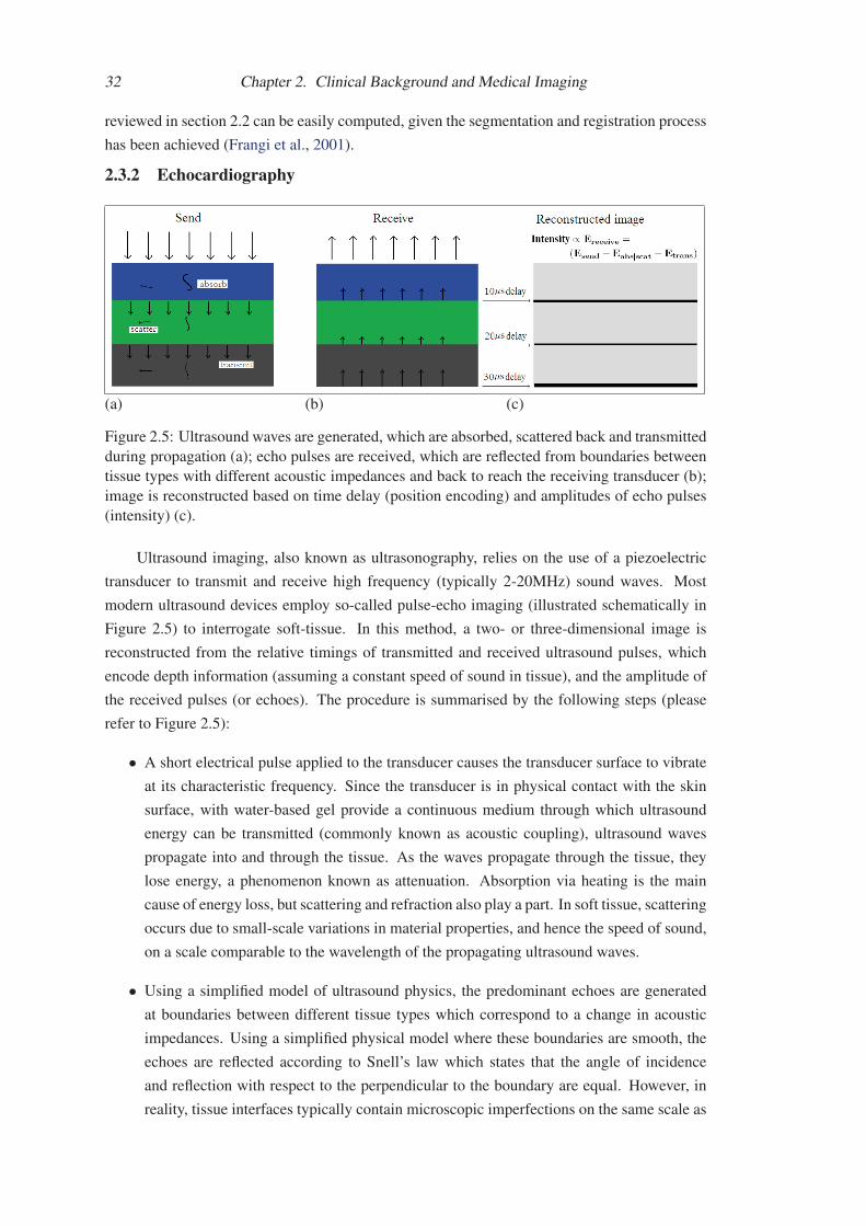
32 Chapter 2. Clinical Background and Medical Imaging
reviewed in section 2.2 can be easily computed, given the segmentation and registration process
has been achieved (Frangi et al., 2001).
2.3.2 Echocardiography
(a) (b) (c)
Figure 2.5: Ultrasound waves are generated, which are absorbed, scattered back and transmitted
during propagation (a); echo pulses are received, which are reflected from boundaries between
tissue types with different acoustic impedances and back to reach the receiving transducer (b);
image is reconstructed based on time delay (position encoding) and amplitudes of echo pulses
(intensity) (c).
Ultrasound imaging, also known as ultrasonography, relies on the use of a piezoelectric
transducer to transmit and receive high frequency (typically 2-20MHz) sound waves. Most
modern ultrasound devices employ so-called pulse-echo imaging (illustrated schematically in
Figure 2.5) to interrogate soft-tissue. In this method, a two- or three-dimensional image is
reconstructed from the relative timings of transmitted and received ultrasound pulses, which
encode depth information (assuming a constant speed of sound in tissue), and the amplitude of
the received pulses (or echoes). The procedure is summarised by the following steps (please
refer to Figure 2.5):
• A short electrical pulse applied to the transducer causes the transducer surface to vibrate
at its characteristic frequency. Since the transducer is in physical contact with the skin
surface, with water-based gel provide a continuous medium through which ultrasound
energy can be transmitted (commonly known as acoustic coupling), ultrasound waves
propagate into and through the tissue. As the waves propagate through the tissue, they
lose energy, a phenomenon known as attenuation. Absorption via heating is the main
cause of energy loss, but scattering and refraction also play a part. In soft tissue, scattering
occurs due to small-scale variations in material properties, and hence the speed of sound,
on a scale comparable to the wavelength of the propagating ultrasound waves.
• Using a simplified model of ultrasound physics, the predominant echoes are generated
at boundaries between different tissue types which correspond to a change in acoustic
impedances. Using a simplified physical model where these boundaries are smooth, the
echoes are reflected according to Snell’s law which states that the angle of incidence
and reflection with respect to the perpendicular to the boundary are equal. However, in
reality, tissue interfaces typically contain microscopic imperfections on the same scale as

2.3. Introduction to non-ionising radiation imaging 33
Figure 2.6: A cardiac ultrasound image from the long-axis view (left) and short-axis view
(right). Red arrows point to shadowing artefacts. Ultrasound image from Guy’s and St Thomas’
Hospital, London.
the wavelength of the ultrasound. In this case, scattering occurs and is the primary source
of echoes in real ultrasound imaging.
• Once the echo pulses arrive at the transducer surface, they generate an electrical pulse,
which is amplified and detected by the probe electronics. It is these signals that are
used to reconstruct the gray-level images: after amplitude modulation, the relative timing
of the received echo and the transmitted pulse are converted into a depth measurement,
perpendicular to the transducer surface, using the relation that (assuming a constant speed
of sound through tissue) the time between the transmitted pulse and corresponding echo is
proportional to twice the depth of the structure producing the echo. Since modern clinical
ultrasound transducers are usually made up of an array of transducer elements, multiple
scan-lines can be generated by repeating this process for different positions along the
transducer surface. This is achieved by activating small contiguous groups of transducer
elements in array in sequence to generate a series of pulses along a focused beam. These
scan-lines then form the columns of a so-called B-mode image. The pixel intensity is
proportional to the amplitude of the received pulse after log compression. As noted above,
ultrasound pulses are attenuated as they propagate. This means that received pulses have
much smaller amplitudes than the initial transmitted pulses generated from the transducer,
but also that echoes from deep structures have a smaller amplitude than echoes from more
superficial structures. To compensate for this effect, a process of amplitude adjustment,
called time-gain compensation (TGC), is used in which the received signal is amplified
according to the depth (equivalent to the receive time) of the received pulses. TGC is
normally adjusted on the scanner by the operator.
• Finally, the scan-lines are mapped to a regular grid and filtered to produce the displayed
image. Clinical B-mode images are typically updated at a rate 5-100Hz, allowing real-
time scanning.
Echocardiography, commonly referred to as simply echo by cardiologists, is ultrasonogra-
phy of the heart. Figure 2.3 (c) shows an echo system used by our collaborating clinical partner
and Figure 2.6 shows an example of a clinical echocardiographic scan. Besides the advantages

34 Chapter 2. Clinical Background and Medical Imaging
of being a safe, non-invasive, inexpensive, and portable imaging modality, echocardiography al-
so has the advantage of enabling real-time imaging, which is extremely important for a dynamic
organ such as the heart and provides useful functional information for studying valve-related
diseases, such as regurgitation, a condition where the blood flows back through the partially
closed valves. The dynamic information from echo is also useful for evaluating wall motion
which provides a clinical indication for the occurrence and severity of coronary heart diseases,
as discussed in Chapter 2.1 and 2.2.
Echocardiography also enables the structure and size of cardiac anatomy to be assessed,
providing information for detecting morphological abnormalities of the heart. However, the
images must be interpreted in the presence of artefacts, such as speckle and acoustic shadowing
(see Figure 2.6). Image noise and artefacts present a substantial challenge for automatic image
processing algorithms. Furthermore, unlike most alternative cardiac imaging modalities, such
as MR and CT, echocardiography has a limited field of view (FOV) determined by the length
of the transducer array and the maximum depth ultrasound penetration (typically, 5-20cm for
cardiac imaging). As a result, echocardiography normally cannot image the whole heart using
a single scan, as shown by the image in Figure 2.6. Subsequently, the value of 3D echocardio-
graphy in terms of a wide FOV is gaining increasing clinical interest. Matrix array transducers
provide a means of acquiring 3D ultrasound image data rapidly from a volume at frame rates
of up to several volumes per second. However, cardiac gating and volumetric compounding
are necessary to maximise the FOV and image quality in practice (Grau and Noble, 2005; Grau
et al., 2007; Yao et al., 2009; Rajpoot et al., 2009b).

Chapter 3
Literature Review and Theory
3.1 Literature review on segmentationThis section reviews the segmentation literature. Section 3.1.1 gives an introduction to segmen-
tation. Section 3.1.2 to 3.1.4 surveys the literature related to three categories of model-guided
segmentation. Section 3.1.5 provides the research direction and the rationale for this direction.
3.1.1 IntroductionIn medical image processing, segmentation is a process to partition one or a series of images into
different regions or to delineate boundaries of these regions. The segmented regions normally
have important information for clinical usages. The goal of segmentation is to extract and
separate the desired information, and the result is a set of new images providing each piece of
the information.
In this review, we will first introduce the theory of threshold, edge detection, and region
growing methods. These methods are data-driven and usually considered as low-level segmen-
tation algorithms (Suri, 2000). This is because the segmentation solely relies on the information
available from the image. Then, we will classify the high-level methods, the model-guided ap-
proaches, into three categories and review the existing works in detail in the following sections.
Threshold: One can use thresholding of intensity values to extract a region of interest.
A successful thresholding requires that the intensity distribution of the region of interest should
not be overlapping with that of other regions in the image histogram. This requirement is
evidently too strong for the segmentation of cardiac MR images. For example, a failure may
occur in the segmentation of myocardium, because the intensity of the myocardium could be
similar to that of the liver as shown in Figure 1.3 (c). Another example is the separation of the
blood pool into different anatomical regions, such as the right atrium and ventricle segmentation
shown in Figure 1.3 (b). The intensity range of the atrial blood cavities could overlap with that
of the ventricular blood cavities. Therefore, prior anatomical knowledge would be needed in
order to defining the boundary between these regions.
Edge detection: Edge detection takes the intensity values of neighbouring points into
consideration when deciding the boundaries between regions. A review and comparison be-
tween a number of algorithms can be found in (Heath et al., 1997). Points with high magnitude
of intensity gradient are usually considered as having a high probability of being edge points.
Canny (1987) assumed that points with local maximal gradient, zero second directional deriva-
tives, should be edge candidates. This assumption makes the detection easier and more robust

36 Chapter 3. Literature Review and Theory
to noise using a technique, known as hysteresis, to protect true edge with low gradient value.
Hysteresis also contributes to producing more continuous contours, to avoid dash-like edges.
Edge detection techniques can be also used as a boundary profile in boundary-searching-based
segmentation (Rouchdy et al., 2007).
Region growing: Region growing incorporates the knowledge that pixels in the same
region are connected and have a similar intensity value. This is also assumed in the procedure
of growing the region. Starting from a selected seed point, the algorithm expands the volume by
assimilating neighbour pixels that match a predefined similarity criterion using intensity mean,
intensity variance, shape smoothness, and a combination of them. The key step of this method
is to define the similarity criterion which usually needs parametrisation to avoid the leaking
problem. Furthermore, the seed point is normally manually selected, and this also could lead to
different results from different observations.
Model-guided: The lower level techniques listed above are mainly driven by the data
themselves without a pre-constructed model for shape guidance. This however makes segmen-
tation too flexible and can result in random and unrealistic shapes due to the noise, artefacts,
and indistinct boundaries presented in the image. Model-based methods utilise the prior in-
formation coming from the models for guidance. These techniques have been widely used in
automatic or semi-automatic cardiac image segmentation. For terminology simplicity, any one
of the deformable models, probabilistic atlases, and intensity atlases is referred to as a model.Based on different usages of the model, we classify the techniques into three groups:
• texture classification using Expectation-Maximisation (EM) algorithm,
• boundary-searching with deformable shape models,
• atlas propagation using image registration.
In the following three sections, we will review the typical works reported in the literature.
Figure 3.1 provides the table summarising these works.
3.1.2 Texture classification using EM algorithmEM segmentation refers to the texture classification methods which employ EM optimisation
to estimate the parameters of a texture label model. In this model, each pixel is assigned with a
classification label. By modelling the intensity distribution of each tissue, the probability of the
labelling can be estimated given the parameters of the model associated with this tissue being
available. For example, it is common to assume that the intensity of a tissue has a Gaussian
distribution, which is defined by the intensity mean and standard deviation. EM is used to max-
imise the likelihood of labelling parameters given the current estimation. In this segmentation,
contextual information is incorporated by means of Markov Random Field (MRF) to improve
the performance and robustness to noise. An average-intensity atlas, known as an atlas of apriori probability maps, is also used for the initial estimation of the parameters.
EM classification methods have been successfully applied in statistical classification for
brain MR images (Leemput et al., 1999; Zhang et al., 2001) where the images are of better
quality (higher signal-to-noise ratio). The intensity classes of gray matter, white matter, and
cerebrospinal fluid are also quite separable in MR images. Lorenzo-Valdes et al. (2003, 2004)

3.1. Literature review on segmentation 37
Met
hod
Seg
men
tation
are
a an
d da
taRes
ults
(m
m)
Com
men
tsLo
renz
o-Val
des
et
al.
(200
3,20
04)
Reg
ion
clas
sific
atio
n us
ing
EM
algo
rith
mVen
tric
les
and
myo
card
ium
se
gmen
tation
fro
m m
ulti-s
lice
cine
MR
2.21
-2.9
9 (m
ean)
Con
s: n
o so
lution
is p
rovi
ded
for
exte
nsio
n to
sep
arat
ion
betw
een
atria
and
vent
ricl
es o
r th
e se
para
tion
of
the
papi
llary
m
uscl
e fr
om m
yoca
rdiu
mLy
nch
et a
l. (2
008)
Reg
ion
clas
sific
atio
n us
ing
EM
algo
rith
m w
ith
prio
rs o
f in
com
pres
sibi
lity
Sam
e as
abo
ve1.
2475
±1.
3369
(m
ean)
1.
8670
(RM
S)
Pros
: th
e in
corp
orat
ion
of
myo
card
ium
inco
mpr
essi
bilit
y pr
ior
know
ledg
e im
prov
es s
egm
enta
tion
per
form
ance
in 4
D c
ases
Con
s: s
ame
as a
bove
Hau
tvas
t et
al.
(200
6)
Act
ive
cont
our
mod
el a
nd
prop
agat
e m
anua
l del
inea
tion
to
othe
r ph
ases
Sam
e as
abo
ve1.
12-2
.64
(RM
S)
Pros
: no
nee
d of
tra
inin
g an
d th
e ap
plic
abili
ty t
o al
l pat
holo
gies
. Con
s: t
he li
mited
aut
omat
ion
due
to t
he u
ser-
inte
ract
ion
to
defin
e an
initia
l con
tour
suc
h as
tha
t of
the
end
-dia
stol
ic p
hase
Pl
uem
pitiw
iriy
awej
et
al.
(200
5)Act
ive
cont
our
mod
el a
nd
prop
agat
e th
e bo
unda
ry o
f a
coni
c e q
uation
mod
el t
o un
seen
dat
a
Ven
tric
le a
nd m
yoca
rdiu
m
segm
enta
tion
fro
m h
igh
reso
lution
rat
MR
N/A
Pros
: a
sim
ple
impl
emen
tation
.Con
s: o
nly
prel
imin
ary
valid
atio
n on
rat
dat
a w
hich
had
a f
ixed
fie
ld-o
f-vi
ew u
nclo
sing
the
hea
rt r
egio
nKau
s et
al.
(200
3,
2004
)Act
ive
cont
our
mod
el w
ith
the
trai
ning
info
rmat
ion
from
the
st
atis
tica
l sha
pe m
odel
and
se
gmen
tation
pro
paga
tion
Myo
card
ium
seg
men
tation
fr
om m
ulti-
slic
e ci
ne M
R
2.28
-2.6
2 (m
ean)
Pros
: th
e tw
o ty
pes
of p
rior
info
rmat
ion,
the
spa
tial
ly v
aryi
ng
feat
ures
and
the
sur
face
con
nect
ivity,
impr
ove
the
rob
ustn
ess.
Con
s: li
mited
acc
urac
y an
d th
e de
pend
ence
on
the
trai
ning
dat
a se
t to
con
stru
ct t
he s
atis
tica
l sha
pe m
odel
van
Ass
en e
t al
. (2
006)
Sam
e as
abo
veLe
ft v
entr
icle
fro
m a
rbitra
ry
orie
nted
MR
1.14
-3.1
9 (m
ean)
Pros
: go
od r
obus
tnes
s cl
aim
ed.
Con
s: n
eed
man
ual i
nter
action
for
initia
lisat
ion
and
limited
ac
cura
cy d
ue t
o th
e lim
ited
fle
xibi
lity
of
stat
istica
l sha
pe m
odel
Ecab
ert
et a
l. (2
008)
Sam
e as
abo
veW
hole
hea
rt s
egm
enta
tion
on
CT
0.82
±1.
00 (
mea
n)Pr
os:
good
acc
urac
y re
porp
ted.
Con
s: t
he v
alid
atio
n is
not
inde
pend
ent
and
the
appl
icab
ility
was
on
ly t
este
d on
dat
a fr
om s
imila
r pa
thol
ogy
Koi
kkal
aine
n et
al.
(200
8)Sam
e as
abo
veW
hole
hea
rt s
egm
enta
tion
2.06
±0.
55 (
mea
n)
(bes
t)It
is a
wor
k on
com
pariso
ns o
f se
vera
l met
hods
to
artific
ially
au
gmen
t th
e va
riab
ility
of
the
stat
istica
l sha
pe m
odel
use
d in
the
se
gmen
tation
. Pe
ters
et
al.
(200
7,
2009
) Sam
e as
abo
veW
hole
hea
rt s
egm
enta
tion
0.76
±0.
30 (
mea
n)Pr
os:
good
acc
urac
y re
port
ed.
Con
s:lim
ited
app
licab
ility
to
sim
ilar
path
olog
y on
ly a
nd t
he
depe
nden
t va
lidat
ion
whi
ch m
ay le
ad t
o bi
as c
oncl
usio
n of
the
ac
tual
ly p
erfo
rman
ce o
f th
e ap
proa
chRou
chdy
et
al.
(200
7)A d
efor
mab
le e
last
ic m
odel
for
se
gmen
tation
pro
agat
ion
Ven
tric
les
and
myo
card
ium
fr
om c
ine
MR
N/A
Con
s: o
nly
test
seg
men
tation
on
four
mic
e da
ta
Lore
nzo-
Val
des
et
al.
(200
2)Reg
istr
atio
n-ba
sed
prop
agat
ion,
fr
om t
he e
nd d
iast
olic
pha
se t
o ot
her
phas
es
Ven
tric
les
and
myo
card
ium
fr
om m
ulti-s
lice
cine
MR
N/A
Con
s: li
mited
acc
urac
y an
d lim
ited
aut
omat
ion
impa
ct (
man
ual
segm
enta
tion
on
one
phas
e be
fore
pro
paga
tion
)
Mitch
ell e
t al
. (2
002)
Reg
istr
atio
n-ba
sed
prop
agat
ion
usin
g ac
tive
app
eara
nce
mod
el f
or
regi
stra
tion
Left
ven
tric
le f
rom
mul
ti-s
lice
MR
2.63
-2.7
5 (m
ean)
Pros
: go
od r
obus
tnes
s an
d w
ide
appl
icab
ility
Con
s: li
mited
acc
urac
y du
e to
the
con
stra
int
from
the
poo
r de
form
atio
n fle
xibi
lity
of t
he m
odel
Lapp
et
al.
(200
4)Reg
istr
atio
n-ba
sed
prop
agat
ion
usin
g st
atis
tica
l def
orm
atio
n m
odel
to
cons
trai
n th
e fle
xibi
lity
of
the
defo
rmat
ion
Ven
tric
les
and
myo
card
ium
fr
om m
ulti-s
lice
cine
MR
4.0±
1.6
(mea
n)Con
s: li
mited
acc
urac
y in
the
leav
e-on
e-ou
t ex
perim
ent
Lotj
onen
et
al.
(200
4)Reg
istr
atio
n-ba
sed
prop
agat
ion
usin
g ac
itve
app
eara
nce
mod
el
with
exte
nded
fle
xibi
lity
Who
le h
eart
seg
men
tation
fr
om c
ardi
ac M
RI
of d
iffer
ent
orie
ntat
ions
2.53
±0.
70 (
mea
n)Pr
os:
exte
nded
fle
xibi
lity
of t
he m
odel
impr
oves
the
acc
urac
y of
th
e se
gmen
tation
met
hods
of
this
kin
dCon
s: t
he v
alid
atio
n w
as d
one
on d
ata
from
hea
lthy
vol
unte
ers
and
henc
e th
e ro
bust
ness
of
the
met
hod
is q
uest
iona
ble
Figure 3.1: Table of the typical segmentation works on cardiac MRI, selected from the literature.
The Result column presents the mean surface-to-surface or point-to-surface segmentation error
(mean) or root mean square (RMS) of the error. The best result of Koikkalainen et al. (2008),
where they compared several augmentation methods to improve the segmentation accuracy, is
presented in this table.
38 Chapter 3. Literature Review and Theory
applied it to the segmentation of ventricles from cine cardiac MR data. Lynch et al. (2008) fur-
ther incorporated the myocardium incompressibility as priors into the 4D segmentation. These
cardiac data were multi-slice short-axis orientated images, covering the heart from the apex up
to the basal planes. The myocardium and ventricular blood cavities could be well separated
based on their intensity. The visual segmentation results in their papers showed that the pap-
illary muscle, a small structure with a similar intensity distribution to the myocardium, was
only partly included into the ventricle cavity. Some cases showed the majority of the papillary
muscle was included into the myocardium. Also, the boundaries of the classified regions were
not as smooth as the surface delineation provided by the other two categories of methods that
will be reviewed in the next two sections. Finally, the classification mainly relies on the dif-
ferent intensity distributions to separate adjacent regions. This raises the question whether the
classification is extensible to the whole heart segmentation of cardiac MRI where the intensity
distributions of the four chambers and the great vessels can be almost identical. To the best of
knowledge, no work has been reported on this attempt.
3.1.3 Boundary-searching with deformable modelsActive contour or snake method (Kass et al., 1988) is a framework which minimises an energy
associated with the current contour. This energy is a linear combination of internal and external
energy terms. The external energy is supposed to be minimal when the active contour reaches
the ground-truth boundary position. The internal energy is supposed to be minimal when the
shape of the active contour has the desired or predefined properties. Active contour is one of
the most popular frameworks in model-based segmentation to deal with objects with complex
shapes such as brain or heart, where a model of the object is used for shape guidance when
defining the internal energy terms. The shape most close to the model is the shape most desired.
Boundary-searching based segmentation achieves automation by deforming the surface of
a pre-constructed model towards the detected boundaries in unseen images, while at the same
time constraining the model within a reasonable shape from the a priori knowledge of the
model. The searching is done by optimising an energy function combining both the external
and internal energy terms, similar to the idea of the active contour model (Kass et al., 1988).
The terms defined within the external energy vary between each research group, but the main
idea is similar and related to the distance between the boundary points of the model and the
searched boundary candidates. The internal energy is more variable, though its definition is
usually related to the shape of the prior model.
The prior model is crucial in this category of segmentation approaches. A number of dif-
ferent representations of this shape model have been used, including manually delineated con-
tours, mathematical models, point distribution models, deformable mesh models, and volumet-
ric models with or without bio-mechanical properties. The works are presented chronologically
for each model representation in the following survey.
Hautvast et al. (2006) addressed the three common challenges presented in automatic
segmentation, providing a useful motivation and discussion for other segmentation frameworks:
(1) the trade-off between decreasing user interaction and providing good initialisation,
(2) the myocardium leaking problem such as to the papillary muscle and liver,
(3) the difficulty of weighting and parametrising different terms in the cost function.

3.1. Literature review on segmentation 39
They reduced the user-interaction to solely defining an initial contour delineation, such as
from end-diastolic (ED) phase, which could be propagated to other phases for automation. The
model is the initial manual delineation, providing guidance for automatic segmentation such
as delineating the boundary between the papillary muscle and the myocardium. The internal
energy is related to the local contour curvature, and the external energy is based on the inten-
sity difference between the reference and unseen images on the perpendicular direction of the
contour.
They did a validation on sixty-nine cine cardiac MR cases from both the short-axis (SA)
and long-axis (LA) orientation. The quantitative validation were only calculated on end-systolic
(ES) phases due to the massive manual work of building a gold standard for all phases, and they
argued that the propagation to other phases should be no worse than the segmentation on the
ES phases. Their segmentation results are presented below, where LV and RV are acronyms of
left ventricle and right ventricle respectively:
Contour εmean(mm) εrms(mm) εmax(mm)SA LV Endocardium 2.23± 1.10 2.64± 1.30 5.00± 2.72SA LV Epicardium 1.84± 1.04 2.27± 1.35 4.70± 3.63SA RV Endocardium 2.02± 1.21 2.63± 1.77 7.87± 8.11LA LV Endocardium 1.82± 0.61 2.31± 0.87 5.76± 2.62LA LV Epicardium 0.92± 0.42 1.12± 0.61 2.38± 2.41
The main advantage of this work is that it does not need a shape training stage; hence it is
applicable to any pathological cases. However, using the manual delineation on the first phase
to initialise the propagation limits the automation as manual delineation of the first phase is
required for each subject.
Pluempitiwiriyawej et al. (2005) used a conic equation to model the ventricle cavity as an
ellipsoid. The internal energy was defined to the contour smoothing term, J(C) =∫C ds, and
the external energy was the combination of the matching function based on regional intensity
and the distance to the detected edges. The profile for defining the optimal edge points was
based on magnitude of image intensity gradient. This model is simple in construction and ele-
gantly formulated in maths for deriving the internal energy. However, more complex modelling
may be needed in order to model the structure of the whole heart.
Medial representation (M-Reps) (Siddiqi and Pizer, 2008) is a more sophisticated tool to
model objects with irregular shapes. Pizer et al. (2003) demonstrated its applicability in image
segmentation for several different applications, but that for cardiac images had not been includ-
ed. Pilgram et al. (2006) built a heart model based on M-Reps, which shows the possibility of
applying M-Rep to this task, but the application to whole heart segmentation, to the best of our
knowledge, has not been reported.
The point distribution model (PDM) is usually reported together with a statistical shape
model (SSM). The SSM is also known as the active shape model (ASM). SSM is constructed
from a training set by means of the principle component analysis (PCA), given that all the
training cases have been mapped to a common space (Cootes et al., 1995). SSM can also be
constructed using other model representations such as the deformable mesh model, volumetric
model, which is also referred to as a statistical deformation model (Rueckert et al., 2003).
SSM assumes the variation of the shape in a group is multi-dimensional Gaussian dis-
tributed. If the shape of an unseen image falls within this distribution, the segmentation can be

40 Chapter 3. Literature Review and Theory
easily achieved by adapting the weights of the dominating modes from the PCA (Mitchell et al.,
2002). The advantage of using this segmentation framework is that the shape of segmented im-
ages is easily guaranteed to be realistic. However, a disadvantage is that the accuracy of the
segmentation may be reduced due to the limited flexibility of the SSM. A more popular way of
using SSM can be summarised as follows (Weese et al., 2001):
• The SSM is firstly used as a global initialisation by adapting the weights of the PCA
modes.
• The flexibility of the shape is then extended by using a local adaptation. In this adaptation,
driving forces are computed from a combination of external and internal energy terms as
an active contour model. The internal energy term, maintaining a realistic shape of the
model, is related to the distance between the current shape to a closest shape within the
variability of the SSM.
Kaus et al. (2003, 2004) proposed a framework to segment the myocardium from multi-
slice cine MR images, and they validated the segmentation on the ED and ES phases. The
profile of detecting boundary points were based on learned ranges of intensity values and in-
tensity gradient. The searching direction was the normal vector of each triangle center of their
mesh model. The external energy was computed based on the distance between the centre of
the triangles and their detected corresponding boundary points. The internal energy penalised
both the distance between the current shape and originally initialised surface shape and the de-
viation between endo- and epi-cardial surfaces. Compared to other works, this study included
two types of prior information, the spatially varying features and the surface connectivity, to
improve the segmentation robustness. However, these constraints may also limit the flexibility
of the deformable model to achieve high accuracy when the model is not closely initialised to
the unseen image at the beginning. The accuracy reported in this study, the mean surface dis-
tance, is given below. The result of the endocardial surface does not seem to evidently report a
statistically significant improvement from the initialisation, considering the standard deviation
is 0.93 mm and the difference of mean is only 0.19 mm.
Error(mm) Mean ED[ES] Standard Deviation MaximumEndocardial surfaceInitialisation 2.47[3.05] 1.87[2.11] 20.92[22.83]Result 2.28[2.76] 0.93[1.02] 13.83[15.43]Epicardial surfaceInitialisation 3.73[4.02] 1.93[2.35] 21.88[22.97]Result 2.62[2.92] 0.75[1.38] 12.35[17.67]
van Assen et al. (2006) reported a ventricle segmentation framework for arbitrarily orient-
ed MR images. They claimed that segmentation method was not limited to the MRI sequence
and widely applicable. First of all, the initialisation of the model to the unseen image was
semi-automatic, which improves the segmentation robustness, but leads to reduced automation.
Furthermore, this study did not report very good segmentation accuracy as a semi-automatic
tool, such as 2.23 ± 0.46 mm mean point-to-surface error for the epicardium segmentation of
short-axis MRI. The limited accuracy was due to the constrained flexibility of the SSM, similar
to the work of Kaus et al. (2003, 2004).

3.1. Literature review on segmentation 41
Ecabert et al. (2008) extended the work of Kaus et al. (2004) and applied it to whole heart
segmentation of CT data. Three technical contributions were presented in this work:
• They addressed the importance and difficulty of localisation, to globally initialise the de-
formable model to the heart location in the CT image, and proposed to use the generalised
Hough transform for this task.
• They introduced the parametric adaptation process which included the piecewise-affine
adaptation. This adaptation significantly increased the flexibility of the model to achieve a
much better initialisation. At the same time, it also had the affinity constraints on the local
regions, and hence was able to maintain the shape of the substructures. This adaptation
did not employ extra internal energy to constrain the shape of the model. They showed
that the mean error mainly improved by the first couple of modes of the PCA model in
Fig. 9 of the paper. The SSM adaptation using all the modes from PCA only achieved 1.7
mm mean accuracy. By contrast, the parametric adaptation further improved it to 1.3 mm.
• They refined the segmentation by optimising both the transformation parameters and the
coordinates of vertices of the mesh model within the competition of the external and
internal energy. They validated their study using the leave-one-out strategy, and the CT
segmentation for whole heart achieved 0.82± 1.00 mm mean surface distance error.
Koikkalainen et al. (2008) investigated different methods of artificially enlarging the
training set for SSM to extend its flexibility. The two best enlargement techniques were the
nonrigid movement and the technique that combines PCA and a finite element model (FEM).
These two methods achieved a mean surface-to-surface error of 2.06 ± 0.55 and 2.06 ± 0.58
mm respectively in the whole heart segmentation which includes four chamber endocardium
and left ventricle epicardium.
Peters et al. (2007, 2009) applied the segmentation framework of Ecabert et al. (2008) to
volumetric cardiac 3D MR images. The validation study on a dataset with limited variety of
heart abnormality reported mean surface distance error of 0.76 ± 0.30 mm, which is the best
result reported to our knowledge. However, the validation was not independent, as the meshes
of gold standard segmentation came from the same mesh model of their segmentation tool with
manual correction. Furthermore, the test data they used had the same or similar pathology,
while a number of other studies were validated using a variety of pathologies. Therefore, an
objective inter-work comparison would be difficult.
The validation in (Ecabert et al., 2008; Peters et al., 2007, 2009) used the data from the
similar pathology where the heart shape might not vary so significantly. In this case, the PCA
model should be expected to be able to capture the variation of the heart shape from the test
data set and thus provide a good initialisation. Therefore, the boundary-searching process was
able to find the optimal boundary within a small searching area. However, the heart shape of
test data in clinics, coming from a variety of pathologies, should vary more significantly as the
test set used in the thesis shows in Chapter 6. The variation of the heart shape presents the main
challenge for the segmentation to achieve a robust automation and hence manual interaction is
used in practical studies (van Assen et al., 2006, 2008).

42 Chapter 3. Literature Review and Theory
Furthermore, the SSM does not naturally guarantee a one-to-one mapping, i.e. a diffeo-
morphic segmentation, from the model to the unseen image. This may contribute to a common
phenomenon that two or more segmented surfaces intersect each other in the result, as the ex-
ample shown in Figure 1.3 (a). Diffeomorphism has the advantage of topology preservation and
is desirable in some applications. Instead, a deformable model which includes physical prop-
erties, such as a biomechanical FEM, can be used to tackle this. The advantage of this model
is that the constraints are implicitly applied from the physical properties of the model itself,
instead of using weighted energy terms. The main concern however is the computation time
for solving FEM equations and the construction of such a model with correct material property
settings.
Rouchdy et al. (2007) generated a deformable elastic template with a nonlinear material
property and applied it to rodent cardiac MRI segmentation. In this work, the mesh model was
first localised to the unseen data using an affine registration. The boundary-searching technique,
using detected Canny edges (Canny, 1987), was then employed as the driving force to locally
deform the mesh to refine the segmentation of local details. The deformation was regularised
by the nonlinear elastic property of the physical model, and hence a more realistic deformation
field was produced during the adaptation. It should be noted that this elastic model was not a
cardiac biomechanical model.
Summary of problemsThe majority of the segmentation works reported good results as we reviewed above. They also
have the advantage of being computational fast. However, there are three technical challenges
of achieving whole heart segmentation, and no work, to our knowledge, has shown the ability
to tackle all of them.
First of all, boundary-searching is normally done within a small area such as along the
normal direction to the model surface in a limited distance, assuming the corresponding edge
point could be found. To ensure the correctness of the assumption, the model needs to be closely
initialised to the true position in the unseen image. This is however a challenging task in the
fully automatic segmentation (Pham et al., 2000) and is difficult to achieve considering the large
shape variability from pathological cases.
Furthermore, the boundary profile, which determines the boundary point candidates, is
mainly based on the information from a small local area of the unseen image such as the inten-
sity value, and the intensity gradient. This profile is however sensitive to intensity inconsistency
such as noise and artefacts, and intensity distribution variations.
Finally, most of these techniques do not naturally guarantee a diffeomorphic segmentation,
which induces two or more segmented surfaces intersecting each other in the result.
3.1.4 Atlas propagation using image registrationSince the boundary-searching based segmentation propagation methods have the difficulties to
deal with all the three challenges mentioned above, an alternative technique is proposed for the
segmentation propagation: the registration-based method. A registration-based segmentation
propagation framework works by registering a pre-constructed atlas, having every region of
interest segmented, to unseen images for segmentation propagation. There are three advantages
of this framework:

3.1. Literature review on segmentation 43
• By using the information based similarity measures such as the mutual information (MI)
or normalised mutual information (NMI), the segmentation propagation becomes less
sensitive to noise, artefacts, and different intensity distributions. This is because in the
registration process, the alignment of each local region is based on a large amount of
information from the whole images.
• The segmentation propagation can retrieve these boundaries with low contrast or that are
not clearly discernible in the unseen images, through the global warping of the atlas.
• To preserve the topology of the heart, the resultant transformation of the registration
should be diffeomorphic, which is nowadays well studied and achievable (Crum et al.,
2005; Rueckert et al., 2006; Vercauteren et al., 2007; Ashburner, 2007).
This segmentation idea has been implemented in brain MR image where the shape from
inter-subjects has less variability. For example, Dawant et al. (1999); Hartmann et al. (1999)
employed the atlas from one single subject as the template for propagation. Rohlfing and Mau-
rer (2005) showed that multi-atlas combined with decision fusion techniques could improve the
segmentation performance, but the atlas still used one single image.
The main difficulty of applying the registration-based framework to whole heart segmenta-
tion is to estimate the appropriate spatial mapping, namely the resultant transformation from the
registration process. Usually, the standard registration scheme uses a global affine registration
to localise the heart, and then apply a nonrigid registration with a transformation containing a
large number of degrees of freedom, such as free-form deformations (FFDs) (Rueckert et al.,
2002), to refine the local details. However, one common issue of the segmentation-propagation
and boundary-based techniques is their relative sensitivity to initialisation, making the algo-
rithms less robust to large shape variability, commonly seen when dealing with pathologies.
Lorenzo-Valdes et al. (2002) proposed to construct a subject-specific atlas for each sub-
ject from ED phase and propagate this atlas to other phase images from the same subject. They
implemented this idea to MRI ventricle segmentation and the registration scheme was the same
as the work of Rueckert et al. (2002). The ED phase provided a good initialisation for local
substructures as well as the global structure to its neighbour phases after a global affine reg-
istration. By using a serial propagation strategy for other phases (normally over ten phases),
they achieved a robust segmentation framework. The limitation of this work is that the subject-
specific atlas was only applied to images from the same subject. Hence, the automation impact
is limited, similar to the work of Hautvast et al. (2006).
Mitchell et al. (2002) constructed an active appearance model (AAM) (Cootes et al., 1999)
and used both the statistical intensity and shape information for the registration. They matched
the AAM to an unseen image by optimising modes of both the textual and shape PCA models.
The used the root mean square (RMS) of intensity difference as the similarity measure. A
good robustness and wide applicability was shown in the paper. In an ideal segmentation, the
AAM should be identical to the unseen image in terms of both the textual and shape after the
registration. However, this is practically difficult in clinics, because the shape variability of
pathological data is large while the flexibility of the PCA model is limited to its training set.
Therefore, the accuracy reported in the paper was not as good as other studies considering the

44 Chapter 3. Literature Review and Theory
interest of segmentation was the left ventricle: 2.75 ± 0.86 mm for the endocardial contours
and 2.63± 0.76 mm for the epicardium using surface-to-surface distance measure.
Lapp et al. (2004) reported a similar work for ventricle segmentation of 3D/4D images.
Unlike the work of Mitchell et al. (2002), they built the AAM using a statistical deformation
model (SDM) (Rueckert et al., 2003). On one hand, they assumed that the registration between
different MR images can be successfully achieved in order to build the SDM. On the other hand,
they employed another registration using AAM to unseen images for segmentation propagation.
Therefore, this method may have either limited segmentation robustness or limited accuracy in
its performance. The results reported in the study were 2.2 ± 1.1 mm for the leave-none-out
scheme and 4.0± 1.6 mm for the leave-one-out test using the mean absolute distance measure
as the segmentation error measure.
Lotjonen et al. (2004) extended the AAM framework to the whole heart, including the
myocardium and the blood cavities of the four chambers, and applied it to cardiac MR images
from different orientations. To extend the deformation flexibility of the AAM, they included the
information of the coordinate of boundaries of all training data and built the information into
a probabilistic atlas to penalise the deformation according to the probability of the appeared
landmarks. The cost function then becomes:
Cost = ENMI + λEmodel
where EMI is the NMI similarity measure, Emodel =1N
∑i log[p(xi)], p(xi) is the probability
of landmark xi mapped to the probabilistic atlas. The template image for registration is the
mean shape and mean texture from the AAM. They argued this mean template should be better
than an image from one single case. The mean texture should be able to improve the signal-to-
noise ratio of the template, but it is questionable whether the mean shape is necessarily closer
to the unseen image when it comes to different pathologies in clinics.
They showed that this extension of flexibility using a probabilistic atlas achieved better
accuracy than only using the statistical shape information constructed either by PCA or inde-
pendent component analysis (ICA) or without any statistical information. The accuracy in mean
surface-to-surface distance to manual segmentation, in millimetre is given below:
Left Ventricle Right Ventricle Left Atrium Right Atrium Epicardium ALL2.01± 0.31 2.37± 0.50 2.56± 0.88 2.93± 1.30 2.77± 0.49 2.53± 0.70
However, the test data used in the work were acquired from healthy subjects whose heart shapes
were supposed to be less variable compared to that from different pathologies. The robustness
of the method is hence still questionable in clinical applications.
3.1.5 Conclusion and research direction
In conclusion to the whole heart segmentation, model-guided approaches are preferred due to
the complexity of this task. The works in the literature mainly focus on propagating segmen-
tation, through either an atlas or a deformable model, to unseen images. The propagation is
mainly done by using the boundary-searching or image registration techniques.
Boundary-searching, commonly used with a deformable model, is the most common tech-
nique published in the past ten years. It has the advantage of a fast computation owing to the
local adaptation only considering the information of a small area. The state-of-the-art imple-

3.1. Literature review on segmentation 45
mentation can segment one volume within one minute using a state-of-the-art personal com-
puter (Peters et al., 2007). However, the limited information for local adaptation also accounts
for the reduced robustness of the boundary-searching process against noise and artefacts, given
that a fully automated tool is pursued.
Registration-based propagation provides an alternative solution for the propagation. The
well developed registration techniques can provide those features desired in whole heart seg-
mentation, such as good robustness against low quality images, good flexibility of the defor-
mation model to achieve high accuracy, and diffeomorphism. With a successful registration
between the atlas and the unseen image, the segmentation of the unseen image becomes avail-
able. Therefore, the research direction of this doctoral work is to develop robust techniques to
achieve this registration.
The main challenge is to model the spatial transformation between the cardiac images from
different subjects. On one hand, the registration needs a flexible modelling method to achieve
high accuracy for the segmentation. On the other hand, the registration needs a shape constraint
on the flexibility to achieve a realistic deformation field, and thus a realistic segmentation. To
obtain a compromise between them, we propose to use an adaptive trade-off in such a way that
the registration starts with strong shape constraints and little flexibility. During the registra-
tion, we increase the flexibility of the model while lessening the constraint. This is done by
using a series of transformation models whose degree of freedom increases slowly along with
the registration process. Correspondingly, the constraints of maintaining the global shape will
gradually relax. According to the registration models, we divided this process into two steps:
initialisation registration and refinement registration.
Figure 3.2: Initialisation using a global affine transformation induces an overlap of local sub-
structures at great vessels, atria and ventricles (left); the refinement based on this generates
erroneous registration results (right). MR data from Guy’s and St Thomas’ Hospital, London.
Initialisation includes global localisation of the heart and local correspondence of sub-
structures such as the four chambers and great vessels. An affine transformation is usually used
for the localisation. For example Rueckert et al. (2002); Lorenzo-Valdes et al. (2002) used a
single global affine registration, and Montagnat and Delingette (2005) applied the affine de-
formation constraint to their deformable model for the initialisation. The affine registration or
constraint maintains the heart shape. However, it is difficult to provide a good local initiali-
sation for substructures. This is demonstrated in Figure 3.2 (left). As a result, an erroneous
segmentation was produced after using a fluid registration for refinement, shown in Figure 3.2
(right).
Refinement registration is done by nonrigid registration with large degrees of freedom. It

46 Chapter 3. Literature Review and Theory
is needed in order to achieve an accurate segmentation, since the initialisation step only gives a
close correspondence between the structures of the images. For the whole heart segmentation,
there are two concerns:
• Our collaborated clinicians prefer to exclude the papillary muscle from the myocardium
and include it into the blood cavities. This was claimed to be more convenient for their
clinical studies. However, the intensity value of the papillary muscle and the myocardi-
um are similar in cardiac MR images. Image registration tends to include the papillary
muscle into myocardium as shown in Figure 3.3 (middle) if no proper prior knowledge
is used.
• The boundary between the myocardium and its adjacent tissues is not always distinct in
our in vivo MR data. The delineation of the epicardium could hence leak to the adjacent
liver tissue, as shown in Figure 3.3 (right).
Figure 3.3: Myocardium segmentation problems: including papillary muscle into myocardium
(middle) and segmentation leaking in epicardium (right). MR data from Guy’s and St Thomas’
Hospital, London.
3.2 Image registration and theoryThis section presents the theory of image registration. Section 3.2.1 introduces the basic knowl-
edge of image registration. Section 3.2.2 focuses on the transformation models. Section 3.2.3
introduces the popular similarity measures. Finally, section 3.2.4 concludes this section and
outlines current problems.
3.2.1 IntroductionMedical image registration is one of the major topics in the medical image computing field (Haj-
nal et al., 2001). Image registration can be considered as a process to compute one or one series
of spatial transformations which map one or one series of medical images to other one with
accurate spatial correspondence. This correspondence means the mapped points from the two
groups of images are from the same anatomical position. The result of an image registration
process can be the transformations, or the transformed resultant images, or both the transfor-
mations and resultant images. The transformations provide spatial mappings between the two
groups of images, and the resultant images are in the same coordinate system as that of the ref-
erence images. The process of image registration provides the capability to fuse or compare the
information of two groups of images in the same coordinate system. The registration images

3.2. Image registration and theory 47
Deform
Image Registration
Reference Image
Resultant Image
Transformation
Floating Image
Figure 3.4: Illustration of image registration
Similarity Measure/Cost Function
Transformation
Optimization/Regularization
Interpolation/Image Modelling
iteration
ReferenceImage
FloatingImage
ResultantTransformation
ResultantFloating Image
Figure 3.5: Framework of image registration
can be acquired from different time points, different modalities, and from different subjects or
populations. Figure 3.4 gives a demonstration of registering two images.
In this work only the registration of two images is studied. An image registration process
includes the following technical components: two intensity images for registration including
the reference image and the floating image, an interpolation method to model spatially contin-
uous intensity images from the discrete grid images, spatial transformation models, a similarity
measure as the cost function, which may also include penalty or regularisation terms, an opti-
misation method which may also have regularisation step to smooth the deformation field, and
the registration result. Figure 3.5 highlights all these components in a flowchart.
Image: The medical images studied in this work are represented in pixels, or referred to
as voxels in three dimensions, on a regular discrete grid. They can be two-dimensional (2D),
three-dimensional (3D), or four-dimensional (4D) which may also be referred to as 3D plus time
dimension (3D+t). The image pair, referred to as the reference image and the floating image,

48 Chapter 3. Literature Review and Theory
can be in the same dimension such as 2D to 2D and 3D to 3D, or in different dimensions such
as 2D to 3D registration. This work only considers images of the same number of dimensions.
Interpolation: Since the images only have intensity values defined on the regular dis-
crete grid points, interpolation is required when there is a need to obtain intensity values be-
tween grid points, such as resampling the images during image registration, or outputting the
transformed resultant image. There are three interpolation methods widely used in image reg-
istration, namely nearest-neighbour interpolation, linear interpolation, and B-spline interpo-
lation. Nearest-neighbour interpolation is the most computationally fast and least accurate
method, while B-spline interpolation is the most accurate and least computationally fast al-
gorithm. There are other higher order interpolation methods that are able to provide better
accuracy, such as sinc interpolation. However, these are less likely to be used in the resampling
of the floating image during the registration process due to its expensive computation. A trade-
off between the run-time and accuracy is needed. Linear interpolation is fast and also provides
good accuracy, while in the registration where high order of differentiability is desired, B-spline
interpolation may be preferred (Thevenaz and Unser, 2000).
In mutual information based registration, partial volume interpolation (Maes et al., 1997)
was proposed to construct the joint histogram table. The computation time for this interpola-
tion is similar to that of the linear interpolation. Pluim et al. (2000) compared the interpolation
artefacts of these two methods and found that partial volume interpolation creates additional
dispersion in the joint histogram while linear interpolation usually decreases the dispersion.
Also the effects of interpolation artefacts to mutual information become more pronounced, e-
specially using partial volume interpolation, when only a small number of sample points are
used for the construction of joint histogram.
With the consideration of smoothing the joint histogram table and thus the resultant prob-
ability density functions (PDFs), it is proposed to use a Parzen window function such as the
Gaussian kernel function (Viola and Wells, III, 1997) or the cubic B-spline kernel function.
Thevenaz and Unser (2000); Loeckx et al. (2006) used the latter because it has the advanta-
geous property of having a local support which is potentially more computationally efficient.
Optimisation: Optimisation is the process of searching for an optimal solution for a
defined problem or function following a certain strategy. In retrospective image registration,
optimising the cost function is commonly done in an iteration scheme. Two methods are in-
troduced here: Powell’s conjugate gradient ascent/descent method and gradient ascent/descent
method.
Powell’s conjugate gradient ascent/descent method (Powell, 1964), also simply referred to
as Powell optimisation, works as follow: In each iteration of the optimisation, it first searches
for optima from the current position P00 sequentially along n directions and at the same time
updates the current position by the new optimal position during each search. The n directions
are normally chosen to be the coordinate axis directions defined by the n transformation pa-
rameters. Then, after finishing all the provided directions, it will then search for an optimum
along the direction of P0n − P00 to replace the current position as P10. P10 is ideally a good
approximation of the true optimum. However, in practice, especially in high dimensional prob-
lems, more iterations are required to ensure that it does not step into a local optimum and then

3.2. Image registration and theory 49
Gradient descent optimisationPowell optimisationP00
P0n
P10
Figure 3.6: Illustration of Powell optimisation (left) and gradient descent optimisation (right).
to guarantee a good accuracy. This procedure is illustrated in figure 3.6 (left). One advantage
of Powell optimisation is that it does not require the cost function to be differentiable and no
derivative is taken for each iteration.
The gradient ascent/descent method, also known as a method of steepest ascent/descent,
searches for the optimum of the cost function along the directions of gradient vectors of the
cost function. At each iteration, the scheme needs to compute the first order derivative of the
cost function and decide the step length to advance, as figure 3.6 (right) illustrates. Ideally,
the optimisation gets closer to the optimum after each iteration and finally converges to the
solution. There are two popular implementations of advancing in each iteration step. One is to
use a regularisation scheme by adaptively decreasing the length in each advancing step:
L(i) =
{l, i = 0
L(i− 1)R(i), i > 0and R(i) =
{1, ∇Ci · ∇Ci−1 ≥ 0
r, ∇Ci · ∇Ci−1 < 0
where l is a user defined length for the first iteration, L(i) is the advancing length at iteration
i, and R(i) is a function of the cost function gradients at current and last iteration steps, ∇Ciand ∇Ci−1, to decide whether use the user defined regularisation rate r ∈ [0.5, 1). The other
scheme is to use the line search routine, advancing along the direction of ∇Ci until reaching a
local optimum (Klein et al., 2007). The scheme needs a technique to search for the optimum
along the gradient direction and the searching operation decides the advancing length.
We adopt the gradient ascent/descent optimisation method with the regularisation schemefor all the registration experiments in this thesis.
Transformation and Similarity measure are the two topics studied in this thesis. Hence,
more detailed introduction and discussion of them will be given in section 3.2.2 and 3.2.3.
3.2.2 Transformation modelsIn most of the nonrigid registration tasks, it is required to use a series of transformation models
to estimate the spatial difference between the two images. According to the linearity of the
transformations, they can be classified into three categories: linear transformations, nonlinear

50 Chapter 3. Literature Review and Theory
transformations, and locally affine transformations.
Linear transforamtions: Linear transformations maintain the linearity and parallel
property of lines after the transformation, hence maintain the global shape of the subject. They
include the following three models:• Rigid transformation, can be defined with 6 degrees of freedom (DOFs) in 3D problems:
three translation parameters and three rotation parameters.• Similarity transformation, can be defined with 9 DOFs in 3D problems: 6 rigid parame-
ters plus 3 scaling ones.• Affine transformation, can be defined with 15 DOFs in 3D problems: 9 similarity param-
eters plus 6 skew ones.Linear transformations have low DOFs and the registration provides limited accuracy when the
images have local deformations. The examples are that when the images are acquired from dif-
ferent subjects, or from different time points of a subject and this subject has local deformations
due to pathological progress. In these situations, nonlinear registration is desired. However, ow-
ing to the global property of linear transformations and being able to initialise the images in the
same physical coordinate with large capture ranges, linear registration is normally done prior to
the nonlinear registration to improve its performance.
Nonlinear transformations: Nonlinear transformations, also referred to as nonrigid or
deformable transformations, have high DOFs. The registration can provide local deformation-
s to align the local difference. Unlikely the linear transformations, it is arguable how realistic
the transformations are for medical image registration. Some groups constructed biomechanical
models to simulate the proper deformations of certain tissues such as the heart (Sermesant et al.,
2003, 2006). The registration using these models is supposed to be more realistic. However, in
practice the implementation of such a validated model could be difficult and the computation of
the registration may be too time consuming. The majority of the works in the literature tried to
employ simplified models to estimate the deformation fields between the images. These simple
models may not relate to the real property of the imaging tissues. The registration techniques
using these transformations include elastic and fluid registration (Christensen et al., 1994; Crum
et al., 2003, 2005), demon registration, and the registration using free-form deformations (FFD-
s).
Among these, the cubic B-spline FFD registration (Rueckert et al., 1999) is one of the
most popular methods due to its easy implement and high efficiency in both modelling and
computation. The cubic B-spline kernel function is defined as follows:
β(3)(a) =
⎧⎪⎨⎪⎩
16(4− 6a2 + 3|a|3), 0 ≤ |a| < 116(2− |a|)3, 1 ≤ |a| < 2
0, 2 ≤ |a|
and a FFD transformation T of x = [x, y, z] in 3D is:
T (x) = x +∑i,j,k
cijkβ(3)(x− φx
ijk
lx)β(3)(
y − φyijk
ly)β(3)(
z − φzijk
lz) ,
where cijk and [φxijk, φ
yijk, φ
zijk] are the displacement vector and coordinate of control point
φijk, respectively, and [lx, ly, lz] is the FFD grid spacing in each dimension.

3.2. Image registration and theory 51
Locally affine transformations: There is a special type of transformations whose DOFs
are between that of the linear and nonlinear transformations, locally affine transformations. A
locally affine transformation model consists of a set of rigid or affine transformations, each of
which is only defined to be effective in a local region, a subvolume of the image. For elsewhere
without a local transformation, an interpolation based on the set of local transformations is
calculated. The transformation model can be expressed as follows:
T (x) =
{Gi(x), x ∈ Vi, i = 1 . . . n
Interpolate {Gi(xi)|i = 1, . . . , n}, x /∈ ⋃ni=1 Vi
,
where {Gi} are the local affine transformations assigned to the corresponding local regions
{Vi}. In the implementation of the registration, a concatenation of a series of such locally affine
transformations is commonly used to model a large displacement with diffeomorphism:
T = T1 ◦ T2 · · ·TN−1 ◦ TN .
The advantage of using these transformations in image registration is that they have both the
global nonlinearity and the local linearity. The global nonlinearity can provide better accuracy
compared to a global affine transformation and the local linearity can preserve the local shape of
substructures. The registration can be applied after a global affine registration to provide a better
initialisation of substructures between the two images for the following nonrigid registration.
3.2.3 Similarity measures
In medical image registration, one of the popular topics is to investigate the intensity-based sim-
ilarity measures for retrospective registration. These intensity-based registration methods em-
ploy the intensity information from the registration images to assess the similarity between the
images. Compared to feature points-based registration methods, this registration takes longer
to compute due to the large amount of information taken into computation. However, this reg-
istration needs less pre-processing on the registration images. For example, the extraction of
feature information is not required, thus no manual processing is involved. Practically, it is able
to provide fully automatic image processing using computers, and hence it is desirable in the
registration-based fully automatic whole heart segmentation framework. This section will pro-
vide theory of three popular similarity metrics that can be directly computed from the intensity
of the images, viz. mean of squared intensity difference, cross correlation, and mutual informa-
tion (MI). Another three methods, intensity gradient difference, normal vector, and local phase
registration will be also introduced here. These metrics are not directly computed from the
intensity values, but instead from some continuously defined features that can be automatical-
ly calculated from the intensity of the images. Therefore, they are also fully automatic and is
useful in registration of ultrasound images where the intensity values are not as reliable as the
imaged features.
Let Ir be an image, referred to as the reference image, If another image, referred to as
the floating image, T the transformation associated with If , S(Ir, If , T ) the similarity measure
of the reference image and the transformed floating image, and x the sample point from the
overlapped volume V .

52 Chapter 3. Literature Review and Theory
Mean of squared intensity difference:
SMSID(Ir, If , T ) =1
|V |∑x∈V
(Ir(x)− If (T (x))2 .
SMSID assumes that the intensity values of corresponding points in the registration images are
the same and their intensity difference is minimised when the images are perfectly matched.
Hence, this metric is not recommended for images with different intensity distributions.
Cross correlation: Cross correlation, also known as correlation coefficient, is a more
robust metric against noisy data and applicable to different intensity distributions with an affine
relationship, i.e. I1 ≈ bI2 + a. It is computed as the ratio between the covariance of the two
sample point sets of the two images and the product of the individual deviations of them: The
cross correlation is:
SCC(Ir, If , T ) =
∑x∈V
[(Ir(x)− Ir)(If (T (x))− IT,f )
]√∑
a∈V (Ir(a)− Ir)2√∑
b∈V (If (T (b))− IT,f )2,
where I =∑
a∈V I(a)
|V | is the mean intensity value of all sample points from volume V .
Mutual information (MI): MI-based similarity metrics have been the most widely used
and most successfully applied algorithms in medical image registration since its invention by
the two groups, viz. Collignon et al. (1995) and Viola and Wells, III (1995). MI is based on
information (entropy) theory and only assumes an intensity class correspondence instead of in-
tensity correspondence between the registration images (see Chapter 8 for detail). This enables
its wide application in both mono-modality and multi-modality registration tasks (Studholme
et al., 1999; Rueckert et al., 1999; Pluim et al., 2003).
There are three forms of MI summarised by Pluim et al. (2003):
MI(Ir, If , T ) =∑r,f
p(r, f) logp(r, f)
p(r)p(f)
= H(Ir) +H(T (If ))−H(Ir, T (If ))
= H(T (If ))−H(T (If )|Ir) ,
where p(◦) are the marginal and joint probability distribution functions (PDFs), and H(◦) are
the marginal and joint entropies of the reference image Ir and transformed floating image If
with transformation T . These three forms in this equation correspond to three interpretations
for the functionality of MI, as follows:
• The first form is related to the Kullback-Leibler distance between two distributions p and
q, defined as∑
i p(i)p(i)q(i) . Accordingly, the MI measure is interpreted as the Kullback-
Leibler distance between the joint intensity probability distribution p(r, f) and the as-
sumed independent marginal distribution p(r)p(f). When this distance is maximised,
the joint distribution is at its least similar to the independent distribution, meaning the
two images are mostly dependent, and thus most similar.
• The second form is related to the joint entropy of the two images, which can be described

3.2. Image registration and theory 53
by the dispersion of the joint histogram table. The less dispersion the joint histogram
is, the better the two images are assumed to be registered. Under this interpretation, the
maximisation of MI is related to the minimisation of the dispersion of the joint histogram
table.
• The final form is related to the mutual uncertainty of the two images. The conditional
entropy H(T (If )|Ir) means the uncertainty of the transformed floating image T (If )
when the reference image Ir is known. While H(T (If ) is the uncertainty of T (If ), MI
can be express as “the amount of uncertainty about image T (If ) minus the uncertainty
about T (If ) when Ir is known” (Pluim et al., 2003).
Studholme et al. (1999) argued that the MI registration only computes the value on the
overlapped volume of the images. However, the MI metric was not invariant to the size of
the overlapped volume. This paper proposed normalised MI, an overlap invariant metric, by
computing the ratio between the sum of the two marginal entropies and the joint entropy:
NMI(Ir, If , T ) =H(Ir) +H(T (If ))
H(Ir, T (If )).
An improved robustness was also demonstrated in their validation.
Intensity gradient difference: Penney et al. (1998) introduced the intensity gradient-
based measures and compared the performance of several similarity metrics when applied to the
registration of a CT scan to a fluoroscopy image of a spine phantom. The gradient difference
measure in this paper was computed as follows:
SGD(Ir, If , T ) =∑
d=1...n
∑x∈V
Ad
Ad +[∂Ir∂xd
(x)− s∂T (If )∂xd
(x)]2 ,
where Ad is the variance of the difference of gradient images in d dimension:
Ad = Variance[ ∂Ir∂xd
(x)− s∂T (If )
∂xd(x)
].
s in both of the two equations above is a scaling factor to compensate the gradient difference
between the two images, and thus is an application or image dependent parameter required to
be determined. The gradient difference was reported to work better than other metrics in the
work of Penney et al. (1998), where structures of soft tissues and thin lines were presented as
differences in the registration images.
Normal vector, normalised vector of intensity gradient: Zhuang et al. (2005); Zhuang
and Gu (2006); Zhuang (2006) proposed to normalise the gradient vectors, referred to as normal
vectors, of images and computed the similarity using the sum of dot product (squared cosine of
the intersected angle θx) of the corresponding normal vector pairs:
SNV (Ir, If , T ) =∑x∈V
cose θx =∑x∈V
[ ∇Ir(x) · ∇T (If )(x)
||∇Ir(x)|| · ||∇T (If )(x)||]e
, (3.1)
where ∇I(x) is the gradient vector of the image at coordinate x.

54 Chapter 3. Literature Review and Theory
Both Griffin (2001) and Karacali (2007) theoretically proved that the local MI or the MI
defined for an infinitesimal aperture at x could be related to θ in the following way:
lims↓0
MI(x) = − ln(| sin θx|) = −1
2ln(1− cos2 θx) .
Therefore, the similarity metrics based on normal vectors can be considered as summing the
local MI over the overlapped volume V . Zhuang and Gu (2006) argued that compared to MI,
the registration using eq. 3.1 was however sensitive to noise in the images due to the locality
of the measure. By contrast, the MI computation benefits from the procedures of histogram
binning and histogram smoothing. Haber and Modersitzki (2006) introduced a regularisation
scheme to compute the normal vector, which is differentiable in iso-intensity areas and the
resultant measure is more robust to areas with small intensity gradient:
Normal Vector(x) :=∇I(x)
||∇I(x)||ε =∇I(x)√
∇I(x)T∇I(x) + ε2.
Biesdorf et al. (2009) proposed to introduce a regularisation factor in the logarithm to reduce
the sensitivity to the noisy driving forces to improve the robustness:
MInew(x) : {log2 |ε+ sin θ|} −→ min .
Local phase: Let I be a 3D image in the spatial domain, the local phase, providing a
quantitative, continuous and contrast invariant description of local features in images, can be
derived using the monogenic signal (Mellor and Brady, 2005; Grau et al., 2007):
φ(x) = atan2(
√√√√ 3∑d=1
(g(x) ∗ hd(x) ∗ I(x))2, g(x) ∗ I(x)),
where, g is a zero mean band-pass filter such as the log-Gabor filter (Grau et al., 2007), convo-
luted with I to constitute the even component of the signal; {hd} are the odd anti-symmetric
filters in the spatial domain, i = 1, 2, 3, whose expression in the frequency domain Hi is:
Hd(u1, u2, u3) =ui√
u21 + u22 + u23.
The local orientation of the signal can be estimated as:
od(x) =g(x) ∗ hd(x) ∗ I(x)√∑3
d=1(g(x) ∗ hd(x) ∗ I(x))2).
Given the local phase, including phase value φ and orientation {od}, a similarity metric can be
computed using the mean square difference of the phase value φ, the cross correlation of φ, the
local phase mutual information (Zhang et al., 2007), or the cosine value of the phase difference
combined with the dot product of the orientation vectors (Grau et al., 2007).

3.2. Image registration and theory 55
3.2.4 ConclusionThe problems of applying existing techniques for the inter-subject registration tasks in the whole
heart segmentation framework are summarised into two categories, as follows:
• Transformation estimation: The traditional registration frameworks use a global
affine transformation for initialisation and refine the local details with a high DOF non-
rigid registration such as the fluid or FFD registration (Rueckert et al., 2002). The ini-
tialisation using a global affine registration is however not good enough for images from
different subjects, where the heart shape varies dramatically. Hence, the first problem is
posed in the initialisation step. Also, in the nonrigid registration, constraints and regu-
larisation processes are needed to achieve a robust result such as to produce a realistic
deformation field between the two registration images. The second problem is posed in
the refinement registration where the shape constraints should be incorporated into the
transformation modelling and registration process.
• Mutual information measure: In the whole heart segmentation framework, the in-
tensity distribution of the intensity image from the heart atlas is commonly different from
that of an unseen image. Hence, MI-based similarity measures are used owing to their ro-
bustness against different intensity distributions. However, the standard MI or normalised
MI measures do not take into consideration the spatial different of each pixel within the
field of view. This may make them less appropriate when the intensity classes of tissues
in the images do not correspond well. It should be noted that this is a general issue of
MI-based registration posed for many applications, instead of solely for cardiac MR reg-
istration. Therefore, the research work on this part is more independent and the proposed
method is applicable to many other applications.

Chapter 4
Local Structure Preservation Using LocallyAffine Registration
This chapter describes the development of registration methods which preserve shapes of lo-
cal substructures. Section 4.1 introduces the locally affine transformation model and existing
registration methods. Section 4.2 elaborates on a new algorithm: the locally affine registration
method (LARM) which keeps global intensity class linkage and diffeomorphism. Section 4.3
describes a method of inverting transformations based on Dynamic Resampling And distance
Weighted interpolation (DRAW). Section 4.4 provides two phantom experiments to demon-
strate the performance of DRAW and LARM. Section 4.5 uses clinical MR data to evaluate the
performance of alternative initialisation methods in whole heart image registration and applying
LARM to the whole heart segmentation. The MR data used in this work and the rationale of
choosing this acquisition protocol are also presented in Section 4.5.1. The conclusion is drawn
in section 4.6.
4.1 Locally affine transformation and registrationRegistration using locally affine transformations, also called piece-wise affine or poly-affine
transformations, is an attractive registration alternative for applications where a single global
affine transformation cannot provide enough accuracy, while a nonrigid registration would in-
correctly affect the local topology due to large shape variations. The registration using locally
affine transformations, namely locally affine registration, assigns a local affine transformation
to each substructure such as four chambers and great vessels in heart images to further initialise
them. This transformation model globally deforms the image, while locally still preserves the
shapes of the pre-defined local regions, the substructures. The registration is normally applied
after a global affine registration to provide better initialisation, which is crucial for some non-
rigid registration to achieve success.
In the following, we firstly review the related work; then we introduce the region-based
registration; and finally we describe the current problems.
4.1.1 Related workHere are the studies on the locally affine transformation model and the registration.
Little et al. (1997), to the best of our knowledge, was the first study to address this transfor-
mation model and discuss its application in medical image registration. In this work, they only
incorporated the rigid substructures and positions of landmarks to interpolate a deformation

4.1. Locally affine transformation and registration 57
field based on the inverse distance weighted scheme (Shepard, 1968):
T (x) =
{Gi(x), x ∈ Vi, i = 1 . . . n∑n
i=1wi(x)Gi(xi), x /∈ ⋃ni=1 Vi
, (4.1)
where Gi is a local affine transformation assigned to a local region or a landmark Vi, and wi(x)
is a normalised weighting factor related to the distance di(x) between x and Vi.
Pitiot et al. (2003) employed the similar idea to hierarchically partition the registration
images into subimages. The corresponding subimages in the image pair were then registered
using the block matching algorithm (Ourselin et al., 2001).
Arsigny (2006); Commowick et al. (2006, 2008) extended the registration method by using
a Log-Euclidean polyaffine framework for the interpolation of a global deformation field from
a set of local affine transformations. This interpolation is done by averaging infinitesimal dis-
placements associated with each affine component. The resultant transformation is obtained by
integrating an ordinary differential equation (ODE).
Zhang et al. (2007) applied the registration framework (Little et al., 1997) to register car-
diac US and MR images. The similarity measure was based on local phase of the images, in-
stead of intensity. This work also provided an automatic method to adaptively detect landmarks
which were used for the definition of local regions.
A common disadvantage of all the studies above is that the registration of each substruc-
ture is done independently of the registration of other structures. This potentially leads to two
problems:
• Each local affine transformation is optimised without taking into account the surrounding
substructures. This passive local process makes the registration less reliable for preserv-
ing the global shape of the organ.
• The registration of each local region does not take the global intensity information of the
images into the computation of the similarity measure. Without this global information,
the registration loses the global intensity class linkage and reduces the robustness against
different intensity distributions. The global intensity class linkage refers to the intensity
class correspondence estimated from the global scale of the two images (see Section 8.1.1
for detail). Zhang et al. (2007) computed local phase based on the whole image, but still
computed the similarity measure of a local registration based on a local area.
Narayanan et al. (2005) proposed a different idea of locally affine transformation and
registration. In this work, each affine transformation Gi is only defined on a centre, called a
seed point xi. A global deformation field is then interpolated using:
Ti(x) = eλ(r)Aeλ(r)S(x− xi) + λ(r′)L+ xi , (4.2)
where, A, S, and L are the rotation, scaling, and translation matrices of the affine transformation
Gi, respectively; λ(r) = e−d2
2σ2 is a function of distance r = ||x − xi|| and σ determines
the locality of Gi: the smaller value of σ the more local effects of this transformation; r′ =||eλ(r)S(x − xi)||. This registration has a set of seed points and each seed point has a set of

58 Chapter 4. Local Structure Preservation Using Locally Affine Registration
Figure 4.1: A diagram demonstrating region-based registration, where {Gi} are local affine
transformations and {Vi} are the corresponding local regions, T is the resultant global transfor-
mation field, procedures REG, Overlap Correction, and Interpolation are defined in the text,.
locally affine transformations which have different values of σ. The resultant transformation is
the concatenation of all these locally affine transformations:
T = T1 ◦ T2 · · ·TN−1 ◦ TN . (4.3)
As each Ti globally deforms the whole image, the registration result does not preserve the shape
of substructures.
4.1.2 Region-based registrationThe region-based registration algorithm, referred to as Rreg, extracts a set of anatomically
meaningful local regions from the reference image and registers each of them to the floating
image (Zhuang et al., 2008a). For the example of registering a cardiac atlas image to an MR
image, the local substructures, including ventricles, atria, aorta, and pulmonary artery, can be
a priori defined in the atlas. To enable each of the local affine registrations, it only includes
the intensity information of a local area, thus loses the global intensity information. Figure 4.1
demonstrates an application of Rreg to the registration of a cardiac atlas and an MR image,
where REG is an affine registration using the NMI similarity measure (Studholme et al., 1999),
Interpolation is the procedure of computing a global transformation field using Eq. (4.1), and
Overlap Correction is a procedure to correct the volumes of pre-defined local regions to avoid
overlap after local affine transformations, as demonstrated in Figure 4.2. A detailed explanation
of Overlap Correction will be given later in Eq. (4.6).
4.1.3 Problem statement• Rreg does not use the global intensity information in the local affine registration. This
means that it loses the global linkage of intensity classes between subimages, and con-
sequantly impairs the robustness against images with different intensity distributions or
from different modalities.
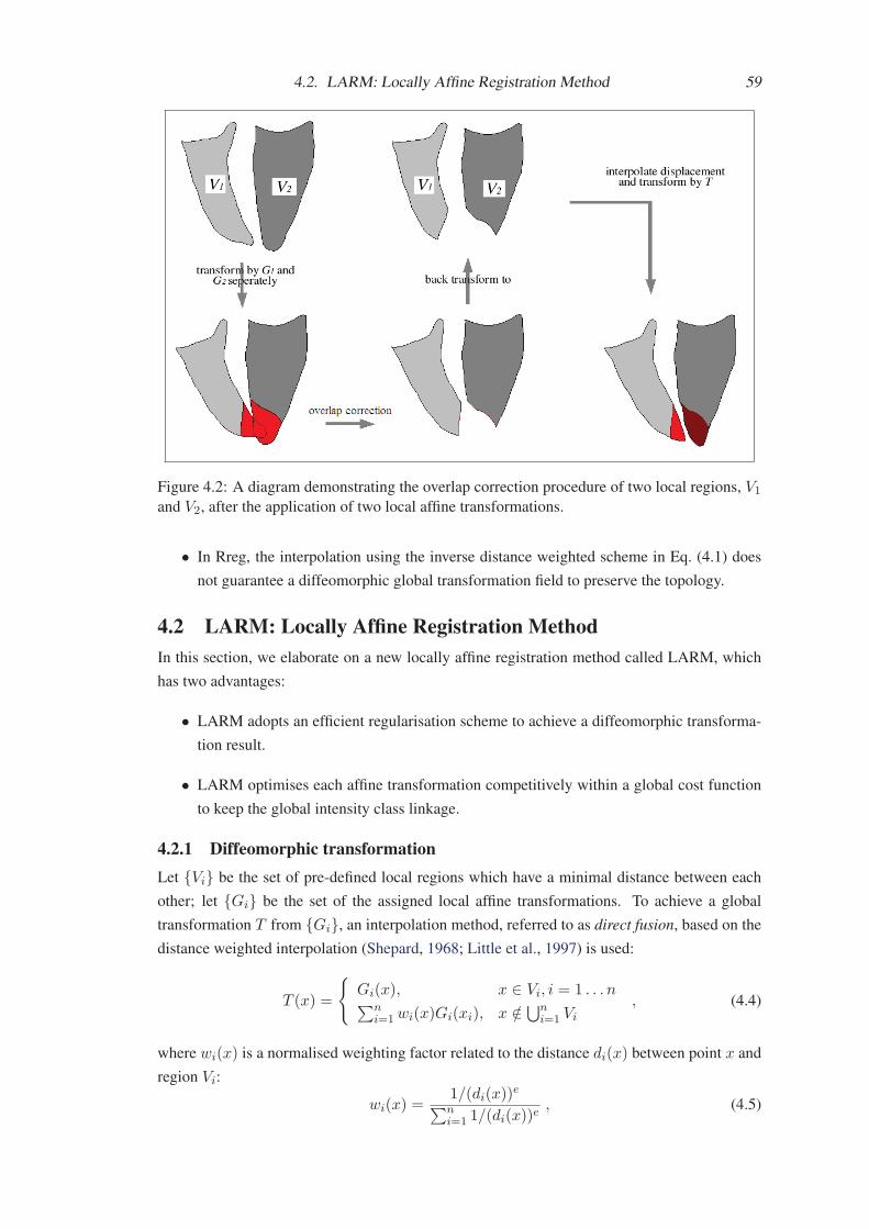
4.2. LARM: Locally Affine Registration Method 59
Figure 4.2: A diagram demonstrating the overlap correction procedure of two local regions, V1
and V2, after the application of two local affine transformations.
• In Rreg, the interpolation using the inverse distance weighted scheme in Eq. (4.1) does
not guarantee a diffeomorphic global transformation field to preserve the topology.
4.2 LARM: Locally Affine Registration MethodIn this section, we elaborate on a new locally affine registration method called LARM, which
has two advantages:
• LARM adopts an efficient regularisation scheme to achieve a diffeomorphic transforma-
tion result.
• LARM optimises each affine transformation competitively within a global cost function
to keep the global intensity class linkage.
4.2.1 Diffeomorphic transformationLet {Vi} be the set of pre-defined local regions which have a minimal distance between each
other; let {Gi} be the set of the assigned local affine transformations. To achieve a global
transformation T from {Gi}, an interpolation method, referred to as direct fusion, based on the
distance weighted interpolation (Shepard, 1968; Little et al., 1997) is used:
T (x) =
{Gi(x), x ∈ Vi, i = 1 . . . n∑n
i=1wi(x)Gi(xi), x /∈ ⋃ni=1 Vi
, (4.4)
where wi(x) is a normalised weighting factor related to the distance di(x) between point x and
region Vi:
wi(x) =1/(di(x))
e∑ni=1 1/(di(x))
e, (4.5)

60 Chapter 4. Local Structure Preservation Using Locally Affine Registration
where di(x) is computed from the closest distance between x and a point in volume Vi. In this
transformation model, a global affine transformation can also be assigned to the boundary of
the region of interest and e is set to 2 for computational efficiency.
However, two reasons can cause non-diffeomorphism by this direct fusion.
• Firstly, the local regions can overlap each other after the individual transformations. To
guarantee non-overlapping, a correction of the local regions is required during the regis-
tration:Vi = G−1
i
(Gi(Vi)−⊕L(Rij)
)= Vi −G−1
i
(⊕L (Rij)) , (4.6)
where, Rij =⋃
i �=j(Gj(Vj)) is the volume of other local regions that Vi should not
overlap after transformations. Operation ⊕L is a morphological dilation with length L,
L=10 mm in our implementation for the cardiac MR application to leave enough space
for the interpolation. It should be noted that when {Gi} are all identity transformations
such as at the beginning of registration, the correction using Eq. (4.6) also guarantees
that there is at least L distance between each local region. Figure 4.2 demonstrates the
procedure of overlap correction.
• Secondly, when the displacements of the local transformation are large, the interpolation
of a global transformation using Eq. (4.4), also referred to as direct fusion, may produce
folding (Arsigny et al., 2005). A regularisation step monitoring the Jacobian JT of the
deformation field is then needed:
JT =n∑
i=1
∂wi
∂x·Gi +
n∑i=1
wi · ∂Gi
∂x= ∇W · GT +∇G · WT , (4.7)
where W = {w1, · · · , wn} and G = {G1, · · · , Gn}. If the determinant of the Jaco-
bian, det(JT ), drops below a threshold (e.g. det(JT ) < 0.5), a new image-pair is then
generated from the original one using the current deformation field and the locally affine
transformation model is reset to the identity transformation for a new optimisation pro-
cess. Therefore, the resultant transformation of the registration is the concatenation of a
series of transformations:
T = Tm ◦ Tm−1 ◦ . . . ◦ T1 . (4.8)
Since all the {Tj |j=1 . . .m} are diffeomorphic, the composed T preserves this property
as well.
4.2.2 Global intensity class linkageTo optimise the local affine transformations, traditional methods register local regions individ-
ually and hence optimise the affine transformations independently (Little et al., 1997; Zhuang
et al., 2008a; Commowick et al., 2008). This independent optimisation however can decrease
the registration robustness due to the loss of global intensity linkage between local regions.
Therefore, we propose to search for the optimal affine transformations within a global scheme,
where each of them is optimised competitively. To achieve this, a global cost function such

4.2. LARM: Locally Affine Registration Method 61
For each optimisation step
Global transformation, F (x) = T ◦G, and T = Tm ◦ Tm−1 ◦ . . . ◦ T1
Optimise global affine transformation GOptimise local affine transformation Gi of Tm, compute derivative using Eq. (4.11)
Regularisation step:
For each region Vi in {Vi}Overlap correction using Eq. (4.6)
If Vi needs correction and is corrected, then
If volume size of Vi is zero, then END registration
else re-compute the distance transformation of Vi for Eq. (4.5)
End of each region Vi in {Vi}If MIN(det(JTm)) < 0.5, then
new a Tm+1, T = Tm+1 ◦ T , and m = m+ 1End of Regularisation
End of Optimisation
Figure 4.3: Pseudo-code for implementing the new locally affine registration method, LARM.
as MI is used and the driving forces are based on the gradient of the MI with respect to the
transformation parameters. The main advantage is that the computation of the cost function and
the driving forces are based on the whole image volume, and hence the global intensity class
linkage is preserved.
The derivative of MI can be obtained by differentiating the entropies, which can be com-
puted from the derivative of the probability distribution function (PDF). Let (l, k) be a joint
histogram bin from the target image It and source image Is, ω be the kernel density estimation
function, the derivative of joint PDF p(l, k) =∑
x ω(It(x)) · ω(Is(T (x))) with respect to a
transformation parameter θi of Gi is:
∂p(l, k)/∂θi =∑
x ω(It(x)) · (∂ω(Is(T (x)))/∂θi)=
∑x ω(It)∇ω(∇Is(y)|y=T (x) · ∂Gi(x)/∂θi)wi(x)
=∑
xW (x)
. (4.9)
Given a point x which has a small value for dj(x), such that dj(x)/di(x) << 1, then wi(x)
tends to zero, making W (x) tend to zero.
Given a volume Ωi and the complementary volume Ωi, we then rewrite the joint PDF
as p(l, k) = PΩi + PΩi, where PΩi =
∑x∈Ωi
ω(It)ω(Is) and PΩi=
∑x∈Ωi
ω(It)ω(Is).
Therefore, the driving force related to the derivative of the entropy becomes:
FH(θi) :=∂H
∂θi= −
∑l,k
(1 + log p(l, k))
(∂PΩi
∂θi+
∂PΩi
∂θi
)= FH(θi)|Ωi + FH(θi)|Ωi
.
(4.10)
where FH(θi)|Ωi = −∑l,k(1+log p(l, k))
∂PΩi∂θi
and FH(θi)|Ωi= −∑
l,k(1+log p(l, k))∂PΩi∂θi
.
Let Ui be a superset volume of Vi such that when x ∈ Ui, one of the follow two conditions can
be met. One condition is wi(x) tends to zero and the other is that x is within the background,
not of interest for the heart registration or segmentation process. Let Ωi = Ui, then FH(θi)|Ωi
is summarised from the contribution of either relatively negligible small forces or less relevant

62 Chapter 4. Local Structure Preservation Using Locally Affine Registration
forces coming from the background. Therefore, the driving force related to the derivative is
computed as:
FH(θi) := FH(θi)|Ωi = −∑l,k
∂PΩi
∂θi(1 + log p(l, k)) . (4.11)
Since (1 + log(p(l, k))), which preserves the global intensity linkage, is constant for all
transformation parameters, the computation complexity of Eq. (4.11) is only O(|Ui∩V |), which
compares with O(|V |) for Eq. (4.10), where V is the volume of the target image. Eq. (4.11) not
only accelerates the run-time, but also blocks driving forces coming from the background such
as the liver and abdomen, where the shape and intensity across subjects vary more significantly.
Figure 4.3 outlines the framework of the proposed LARM and describes the pseudo-code
of our implementation. A global affine transformation is composed with the concatenated T for
the global transformation. The regularisation step includes the overlap correction and monitor-
ing Jacobian for T concatenation.
4.3 DRAW: Dynamic Resampling And distance Weighted interpo-lation
In this section we introduce a generic method for inverting dense displacement fields using
Dynamic Resampling And distance Weighted interpolation (DRAW).
reference image (space) floating image (space)
(a)
(b)
(c)
Figure 4.4: DRAW using inverse distance interpolation from forwardly transformed scatter
points (a); resampling more points within a pixel when the transformation field causes ex-
pansion (b); resampling more points in other directions when the transformation field causes
anisotropic contraction (c) in one direction.
Let T be a diffeomorphic transformation, mapping a coordinate t in reference image space
to a coordinate s in float image space, i.e. s = T (t). To compute the inverse transformation

4.3. DRAW: Dynamic Resampling And distance Weighted interpolation 63
T−1 of T , we extend the scatter-point and distance-weighted scheme (Crum et al., 2007) to
directly interpolate t = T−1(s) for s. Given {si}, a set of close scatter points of s as the light
green points in Figure 4.4 (a), the interpolated inverse transformation TI(s) is computed as:
TI(s) = s+∑i
w(si) · (ti − si) , (4.12)
where {si} are points transformed by T from the point set {ti} in the reference image space
and w(si) is the normalised weighting function computed from the distance between si and s
(refer to Eq. (4.5) for detail). It is assumed that an accurate estimation can be achieved given
the following two conditions stand (for simplicity word pixel is used for both the 2D and 3D
image element):
• Condition 1: One closest point si can be found from each octant (3D) or quadrant (2D)
of s within one pixel dimension.
• Condition 2: The {si} should be transformed from the scatter points {ti} which are all
within the volume of one pixel size.
As shown in Figure 4.4 (a), the inverse transformation of point s, the red point in the float-
ing image, can be interpolated from its neighbouring green points {si} which are transformed
from the green points {ti} in the target image. In a diffeomorphic transformation field T , the
ground truth T−1(s) and the interpolated inverse transformation TI(s) should both be within
the volume enclosed by {ti}, i.e. the red area in Figure 4.4 (a). We assume this because the
algorithm is designed to invert dense displacement fields, and the deformation within the pixel
in the target image may not have detailed definition and can be simply estimated as an affine
transformation. Therefore, the interpolation error |TI(s) − T−1(s)| should not be larger than
the diameter of the enclosed volume.
Two situations make it difficult to meet these two conditions:
• Firstly, if T represents deformational expansion at {ti}, then the scatter points {si} can
be too distant from s (shown in Figure 4.4 (b)): the pixel-size volume Vt enclosed by the
vertex points, the dark green points {ti}, are sparsely transformed into a bigger area Vs
in the floating image space, where a grid point s lies. In this case, one may not be able
to find any of the sparse points required in Condition 1 for the interpolation of TI(s). To
obtain this point set, we propose to resample more points within Vt and transform them
to the floating image space, as shown in the Figure 4.4 (b). The number of resampled
points, Se, is estimated as:
Se = max(1, |J : e|) , (4.13)
where, J is the Jacobian matrix of T and |J : e| = |e × J × e|. The symbol |J : e|represents the volume change in the direction of e, where e is the standard basis of the
Euclidean space �d.
• Secondly, if T represents anisotropic contraction at {ti}, then the scatter points {ti} may
not be within one pixel dimension in the reference image space, as shown in Figure 4.4

64 Chapter 4. Local Structure Preservation Using Locally Affine Registration
(c): if |J : ej |/|J : ek| > 1, the closest scatter points {si} of s are mapped from their
corresponding points {ti} which are the dark green dots in Figure 4.4 (c). The enclosed
volume Vt by point set {ti} is not within one pixel dimension and hence the interpolation
using Eq. (4.12) violates Condition 2. To improve this situation, we propose to resample
more points in the other orthogonal directions inside Vt to provide a closer scatter point
set {si} and a corresponding point set {ti} from one pixel dimension:
Sej =∏k
max(1, |J : ej |/|J : ek|) , j, k = 1, 2, . . . , d . (4.14)
Combining Eq. (4.13) and 4.14, we get the number of resample points needed from the
volume of a pixel:
Sej = max(1, |J : ej |) ·∏k
max(1, |J : ej |/|J : ek|) , j, k = 1, 2, . . . , d . (4.15)
4.4 Phantom data experiments4.4.1 Experiment-1: DRAW for inverting transformationsData and experimental setup
(a) (b) (c) (d)
Figure 4.5: Phantom data used to generate dense displacement. (a) shows a rigid box in a
fixed field; (b) shows the deformation field when the rigid box rotates 85 degrees; (c) shows the
deformation field when the rigid box scales down to half size in one direction and rotates 10
degrees; (d) shows the deformation field when the rigid box scales up to twice the original size
in one direction and rotates 10 degrees.
In this experiment, three groups of transformations are generated and then inverted by
DRAW. The first group is a set of more generic dense displacements used to assess the overall
performance of DRAW. The last two groups are specifically designed affine transformations,
anisotropic scaling-down and scaling-up, which are used to evaluate the performance of DRAW
in scaling situations.
The image used to generate the transformations is shown in Figure 4.5 (a) and is of reso-
lution 401 × 401 × 3 and voxel size 0.5 × 0.5 × 0.5 mm. The assumed reference and floating
images in the procedure of inverting transformations have the same resolution and voxel size.
The first group of transformations are generated by rotating the central rigid box and fix-
ing the boundaries of the reference image. By using a set of rotations from 5 to 85 degrees,
seventeen dense displacements are created using Eq. (4.4) to interpolate them as locally affine

4.4. Phantom data experiments 65
(a)
(b)
Figure 4.6: The scales of the inverse-consistency error with applied rotation (a) and scaling (b).
transformation fields. Each displacement field includes a rigid rotation in the centre and non-
linear expansions and contractions elsewhere. Figure 4.5 (b) shows the displacement of using a
rotation of 85 degrees.
The second group is generated by scaling down the rigid box in one direction and rotating
it 10 degrees. This group has 7 displacement fields using the scaling values of 0.9, 0.7, 0.5, 0.4,
0.3, 0.25, and 0.2. The mean magnitude ranges from 3 mm to 8 mm. Figure 4.5 (c) shows the
displacement of using a scaling value of 0.5.
The third group is generated by scaling up the rigid box in the x-axis direction and also
has 7 displacement fields using the scaling values of 1.5, 2.0, 2.5, 3.0, 3.5, 4.0, and 4.5. The
mean magnitude ranges from 6 mm to 36 mm. Figure 4.5 (d) shows the displacement of using
a scaling value of 2.

66 Chapter 4. Local Structure Preservation Using Locally Affine Registration
ResultsThe error is computed using the inverse-consistency (IC), |T (TI(s)) − s|, within the floating
image space. Both the mean and maximal values are recorded for each case. Figure 4.6 (a)
presents the IC errors of inverting the first group of transformations. The errors are plotted
against the mean of transformation magnitude of each displacement field. Figure 4.6 (b) gives
the IC errors of inverting the second and third groups of transformations. In the latter two
groups, only the points within the central rigid box area are taken into account when computing
the IC error in order to focus on the error caused by anisotropic scaling. The errors are plotted
against the scaling magnitude. It should be noted that the magnitude of a down-scaling value is
computed from its inverse for example the magnitude of 0.2 is 5 (1/0.2).
ConclusionThe maximal errors of all three groups are less than the voxel size, which is however not the case
for the currently reported methods surveyed in Crum et al. (2007). In addition, the maximal IC
errors in the first group reach the largest value at a 45-50 degrees rotation, instead of 85 degree
which has the largest magnitude of displacement, and the mean errors tend to converge from the
position of 45-50 degrees. This indicates that the IC error does not necessarily increase accord-
ing to the increased magnitude of displacements. Finally, in the last two groups, the maximal
IC errors by up scaling transformations are more stable than by down scaling transformations,
even though the transformation magnitudes of down scaling are much smaller.
4.4.2 Experiment-2: LARM vs region-based registration
(a) (b) (c) (d) (e) (f)
Figure 4.7: Floating image (a), subimages (within red line) of the left bar ML (b) and the right
bar MR (c); reference image (d) as registration task one, reference image (e) as registration
task two, reference image (f) as registration task three.
Data and experimental setupThe data used in this experiment are shown in Figure 4.7. The floating image and three reference
images all have two local regions, referred to as left and right bars. The registration tasks are
simulated to multi-modality since the intensity distribution of the floating and reference images
are different.
The purpose of this experiment is to demonstrate the advantage of keeping global intensity
class linkage in multi-modality registration. Both Rreg and LARM are employed to register
these three tasks and assess their performance based on the registration results. Two locally
affine transformations are assigned to the left and right bars. For Rreg, the subimages ML and
MR are defined as the rectangular areas of the bars with a morphological dilation of 20 mm,
as shown in Figure 4.7 (b) and (c). The overlap correction is also used for Rreg in the fusion of
the locally affine transformations. For LARM, the area (volume in 2D) {Ui} used in Eq. (4.11)

4.5. Cardiac MR data experiments 67
Tas
k-t
hre
eT
ask
-tw
oT
ask
-on
e
(a) (b) (c)
Figure 4.8: Overlapping of the reference and floating images of the three registration tasks: (a)
before registration; (b) after registration using LARM; (c) after using the region-based registra-
tion (Rreg).
is also defined to the same size as that of ML and MR.
The registrations use NMI similarity measure and gradient ascent optimisation scheme.
Results
Figure 4.8 shows the registration results of the three tasks using LARM (b) and Rreg (c). Both
have achieved success in task one and two, but Rreg failed in task three while LARM succeeded
attributed to the advantage of maintaining global intensity class linkage. Figure 4.9 gives the
inverse transformations of the three diffeomorphic fields from the registration results of LARM.
Conclusion
This experiment has demonstrated the advantage of LARM over Rreg in registering images
with different intensity distribution. LARM has achieved a success in task three thanks to the
global intensity class linkage, which helped register the right bar when its position is initially
far away in the reference and floating images. Furthermore, LARM demonstrated the ability of
achieving diffeomorphic registration.
4.5 Cardiac MR data experimentsThis section describes the application of LARM and Rreg to cardiac MR data. The registration
in these experiments uses NMI similarity measure and gradient ascent optimisation scheme.

68 Chapter 4. Local Structure Preservation Using Locally Affine Registration
Inver
seF
orw
ard
(a) (b) (c)
Figure 4.9: Deformation meshes of the registration results of LARM: (a) of task one; (b) of task
two; (c) of task three. Upper row is the forward transformations and lower row is the inverse
transformations using DRAW.
4.5.1 MR data used in this thesisThis PhD work mainly focuses on volumetric, isotropic cardiac magnetic resonance (MR) im-
ages with whole heart coverage using a novel MR imaging (MRI) sequence developed at the
Imaging Science Division, King’s College London (Uribe et al., 2007). This sequence is the
balanced steady state free precession (b-SSFP) for whole heart imaging. The imaging has either
one (ED phase) or two (dual phases) trigger delay (s), with a preview T2 preparation and fat
saturation pulse. A 3D triggering b-SSFP turbo field echo (TFE) sequence (with arrhythmia
rejection) has been modified in order to enable the acquisition of selected cardiac phase(s) at a
user defined time. The sequence has been implemented on 1.5T clinical scanners (Philips Med-
ical System, Best, The Netherlands), shown in Figure 2.3 (a), equipped with 32 independent
receive channels, shown in Figure 2.3 (b), at Guy’s Hospital and St. Thomas’ Hospital, Lon-
don. For both cardiac phases, a fat saturation and T2-prep pulses (14) are used to null fat and
to increase the contrast between blood and cardiac muscle. A free breathing scan is realised by
enabling one navigator beam before data acquisition and the trigger delays of the end-diastolic
phase is selected manually with a preview T2 preparation and FAT saturation pulse. The gating
window for the free-breathing scan is controlled to be around 6 mm in volunteers given they
have received a breath-with-regular-pattern training. However, this is not guaranteed for the pa-
tient data acquisitions and the gating window is normally set to larger value in order to reduce
the acquisition time. It should be noted that a wider gating window means less acquisition time
but more pronounced artefacts. Table 4.1 gives the parameters of this sequence.
All the cardiac MR data used in this doctoral work were acquired at Guy’s Hospital andSt. Thomas’ Hospital, London.
Rationale of using the sequence The use of this 3D SSFP sequence in cardiac MRI is be-

4.5. Cardiac MR data experiments 69
Table 4.1: The parameters of the 3D whole heart MRI sequence.
Field of view ∼ 280× 240× 140 mm
Acquired resolution ∼ 2× 2× 2 mm
Reconstructed resolution ∼ 1× 1× 1 mm
No. of slices 110 - 180
TR/ TE ∼ 3.8 ms/ ∼ 1.9 ms
TFE factor 15 - 20
Sense 2 anterior posterior 1-1.5 right left
Flip angle ∼ 60 degrees
No. of phases 1 (ED phase) or 2 (dual phases)
Trigger modality Trigger
coming routine clinical practice and is used increasingly in clinical studies, particularly where
it is important to get accurate information about the geometry of the cardiac chambers. The
advantage of using this sequence is that the acquired images are isotropic and of high reso-
lution. The interpolation of these images can more accurately interpret the geometry of the
heart, which compares advantageously with the data from the standard multi-slice or breath-
hold multi-chunk MRI sequences. The multi-slice cine MRI is widely used in routine clinical
practice. However, it provides limited coverage of view to the ventricles and is used for as-
sessment of regional and global ventricular function. There are many works that describe the
segmentation of these multiple 2D cine SSFP images and their focus remains on the assessment
of ventricular function rather than cardiac geometry.
This 3D SSFP sequence has been compared to the state-of-the-art multi-slice sequence
by Uribe et al. (2008). Comparable results have been found for the quantification of cardiac
volumes and functions. The correlation values were shown to be greater than 0.95 and no
significant difference was recognised for stroke, end-systolic, or diastolic volumes in either of
the ventricles (Uribe et al., 2008).
4.5.2 Experiment-3: Ventricle segmentation using Rreg
Figure 4.10: Atlas image and the ventricle segmentation labels superimposed on the MR image.
Data and experimental setupIn this experiment, ventricle segmentation is achieved by registering an atlas image to unseen
images. Two registration schemes are used and their results are compared:

70 Chapter 4. Local Structure Preservation Using Locally Affine Registration
Table 4.2: Segmentation accuracy of Rreg+Fluid using surface distance measures. This table
also gives the percentages of error scales: 0-2 mm, 2-5 mm, and > 5 mm.
(mm) 0-2 2-5 > 5 Mean STD
Volunteers left ventricle endocardium 94% 4% 2% 0.8± 0.2 0.9± 0.4right ventricle endocardium 92% 6% 2% 0.9± 0.1 0.9± 0.3left ventricle epicardium 80% 15% 5% 1.2± 0.2 1.2± 0.3
Patients left ventricle endocardium 67% 22% 11% 1.8± 0.6 1.7± 0.9right ventricle endocardium 60% 23% 17% 2.2± 1.0 1.7± 0.8left ventricle epicardium 70% 11% 9% 1.6± 0.4 1.4± 0.3
• An affine registration for initialisation and a fluid registration for refinemen-
t (Affine+Fluid);
• An affine registration for localisation, then Rreg to further initialise the two ventricles,
and finally a fluid registration for refinement (Rreg+Fluid).
The fluid registration is based on Crum et al. (2003, 2005) with a force mask applied to exclude
the forces generated from the background (Zhuang et al., 2008a).
The atlas image comes from a cardiac MR image which was acquired from a healthy
volunteer. The substructures, including the left ventricle blood cavity, right ventricle blood
cavity, and the myocardium, have been manually delineated from the MR image. Figure 4.10
shows the corresponding segmentation labels superimposed on the MR image. Another eight
MR images from four healthy volunteers and four Tetralogy of Fallot patients are tested as the
unseen images. Each of them has a manual segmentation, regarded as gold standard.
The segmentation error is only assessed on the left ventricle endocardium, left ventricle
epicardium, and right ventricle endocardium of the heart. Two types of measures are used to
assess the accuracy of the segmentation results.
• Surface distance measures: The mean and standard deviation (STD) of the surface dis-
tance between the automatic segmentations and gold standard are computed.
• Volume measures: The volume difference,|Vgold−Vseg |
Vgold, and the volume overlap (Crum
et al., 2006),Vgold∩Vseg
Vgold∪Vseg, between the segmented volumes Vseg and gold standard Vgold
are computed.
ResultFigure 4.11 (a) displays the mean and STD of the surface distance measures. The mean surface
distance by Rreg+Fluid is 1.0 ± 1.0 mm on the four volunteer data, and 1.6 ± 1.8 mm on the
four patient data; the errors of the patient and volunteer data by Affine+Fluid are 1.3± 1.4 mm
and 2.0±2.0 mm, respectively. Figure 4.11 (b) plots the mean of volume difference and overlap
volume measure: again Rreg+Fluid has a better result than Affine+Fluid. With an initialisation
of the substructure, the Rreg+Fluid scheme performed better, though the improvement was not
evidently very significant.
Finally, Table 4.2 gives the detailed error distribution of the segmentation result using
Rreg+Fluid: the percentage of points whose distance is within 0 to 2 mm, 2 to 5 mm, and more

4.5. Cardiac MR data experiments 71
(a)
Healthy Data by Rreg+FluidPatient Data by Rreg+FluidHeathy Data by Affine+FluidPatient Data by Affine+Fluid
Healthy Data by Rreg+FluidPatient Data by Rreg+FluidHealthy Data by Affine+FluidPatient Data by Affine+Fluid
(b)
Figure 4.11: The mean surface distance distribution and standard deviation of the surface dis-
tance from healthy volunteer data and patient data (a); and the average volume difference and
volume overlap of them (b). This figure shows the difference between the segmentation results
by using Affine+Fluid and Rreg+Fluid.

72 Chapter 4. Local Structure Preservation Using Locally Affine Registration
than 5 mm. The mean and STD values of the surface distance of each local region are also
presented in Table 4.2. The results indicated that the segmentation of patient data was more
difficult than that of healthy volunteer data. Several facts contribute to this difficulty, including
the lower image quality, the larger variations of the heart shape, and the larger inter-observer
variations of the definition of the indistinct boundaries in the gold standard segmentation.
Notice that we group the errors using the thresholds of 2 and 5 mm mainly based on thefollowing three observations: Firstly, the acquisition resolution of the MR data is 2 × 2 ×2 mm; secondly, most of the maximal point-to-surface distance errors between the manualsegmentation and gold standard segmentation from cardiac MR slices are between 1 to 3 mm(Hautvast et al., 2006); finally, the mean point-to-surface distance in the connection areas isbetween 4 and 6 mm which is shown in Figure 6.7 in Section 6.4.4. The first two observationscontribute to the selection of threshold 2 mm, whilst the last one contributes to the selection of5 mm. This error grouping strategy will be used in other experiments throughout the remainderof the thesis.
ConclusionThis experiment demonstrated the advantage of using a locally affine transformation model
to further initialise the substructures of an object. The fluid registration benefitted from the
initialisation of Rreg. Since it did not show a statistical significance of improvement, in the next
experiment we will employ more data to compare the performance using different initialisation
techniques.
4.5.3 Experiment-4: Initialisation in whole heart segmentation
Figure 4.12: Atlas image and the segmentation labels of anatomical substructures superimpos-
ing onto it.
Data and experimental setupThe purpose of this experiment is to demonstrate the difference of performance of the three
initialisation methods that can be used in a registration-based whole heart segmentation frame-
work:
• A global affine registration (Affine).
• Rreg after an affine registration (Rreg).

4.5. Cardiac MR data experiments 73
• LARM after an affine registration (LARM).
The atlas image is the same as that used in Experiment-3, but using 7 substructures to
define the local affine transformations: the left ventricle, right ventricle, left atrium, right atrium,
pulmonary artery, ascending aorta, and descending aorta, as shown in Figure 4.12. Another 18
data are used as unseen images to register to the atlas image. These images have been manually
delineated of the endocardium of the four chambers and the epicardium of the left ventricle.
The accuracy of registration is assessed by the surface distance between each of them after the
registration.
Figure 4.13: The registration accuracy of the three initialisation methods.
ResultFigure 4.13 plots the registration accuracy for each local region and all the surfaces as one
measure, referred to as Whole Heart. The mean errors of Rreg and LARM were better than that
of Affine in all structures. Also the improvement was significant, as the paired t-test p-values
of the Whole Heart errors were both PAffine,Rreg < 0.001 and PAffine,LARM < 0.001. This
was the courtesy of using the prior information of the local substructures for the initialisation.
The mean accuracy of Rreg was shown to be no worse than that of LARM and the paired t-test
p-value of the Whole Heart errors was PLARM,Rreg = 0.90. In the case of the left ventricle,
Rreg actually performed better. The reason is that the left ventricle region has a large volume
and the contrast between the blood pool, myocardium, and background is good in this area.
However, from the standard error of the mean, the standard deviation of the mean values of all
cases, which indicates the variance of the mean and the robustness of the registration, LARM
demonstrated the best result and Rreg did not always outperform Affine. For example, in the
left atrium, Rreg had a large standard error of the mean due to some failure cases. One case is
defined as a failure when the error of the registration result is worse than the error before the
registration. The reason that Rreg performed less consistently in the left atrium was that the left
atrium had relatively smaller volume size and could be poorly initialised solely using a global

74 Chapter 4. Local Structure Preservation Using Locally Affine Registration
affine registration. Without the global intensity information, Rreg was more likely to step into
a local optimum.
ConclusionThis experiment demonstrated that locally affine registration can improve the initialisation of
local regions, confirming the conclusion from Experiment-3. In addition, LARM is a better
choice than Rreg because it provides better robustness. In the next experiment, we will demon-
strate the advantage of a better initialisation in a whole heart segmentation framework.
4.5.4 Experiment-5: Whole heart segmentation using LARMData and experimental setupThe purpose of this experiment is to compare the whole heart segmentation result using the
initialisation of LARM and the traditional initialisation of a global affine registration. The
refinement is again the force-mask fluid registration (Zhuang et al., 2008b). The atlas image
and unseen data are these used in Experiment-4. The two registration schemes to be compared
are:
• An affine registration for initialisation and a force-mask fluid registration for refinement
(Affine+Fluid).
• An affine registration for localisation, then LARM to further initialise the substructures,
and finally a force-mask fluid registration for refinement (LARM+Fluid).
Result
Table 4.3: Segmentation accuracy after each registration step and the p-values of the paired
t-test between the errors of the two registration schemes: Affine+Fluid and LARM+FLuid.
Unit (mm) Affine LARM Affine+Fluid LARM+Fluid P-value
Left Ventricle 5.9± 1.3 4.4± 1.4 3.3± 2.0 2.4± 1.1 0.010
Right Ventricle 4.0± 2.3 3.2± 1.5 3.3± 3.7 2.6± 1.5 0.217
Left Atrium 4.7± 1.6 2.9± 1.0 3.0± 2.0 1.9± .78 0.043
Right Atrium 5.1± 2.5 3.2± 2.1 4.3± 4.7 2.4± 2.7 0.111
Epicardium 4.4± 2.1 1.7± .32 2.3± 1.7 1.3± .21 0.023
Whole Heart 4.1± 1.6 2.8± .40 2.7± 1.7 1.8± .42 0.026
Table 4.3 presents the accuracy of each substructure after using the two initialisation meth-
ods and the two corresponding segmentation frameworks, and the p-values of the two tailed,
paired t-test between the two groups of segmentation results. The fluid registration performed
significantly differently after the initialisation of LARM: the mean Whole Heart segmentation
error of LARM+Fluid (1.8 ± 0.42 mm) was more than twice the standard deviation smaller
than that of Affine+Fluid (2.7 mm) and PWholeHeart = 0.026. In particular the segmenta-
tion of the epicardium of the left ventricle, the mean error of Affine+Fluid (2.3 mm) was more
than three times the standard deviation smaller from that of LARM+Fluid (1.3 ± 0.21 mm)
and PEpicardium = 0.023. However, the p-values of Right Ventricle (0.217) and Right Atrium
(0.111) did not show evidence of significant difference between the two segmentation schemes,
though the mean errors of LARM+Fluid were both smaller than those of Affine+Fluid.

4.6. Conclusion 75
It should be noted that the errors of each category are considered as normally distributed inthe t-test. The assumption is based on the argument that this normal distribution is commonlyaccepted and the t-test is expected to be more accurate than using the Wilcoxon test whichdoes not require the test groups to be normally distributed and may produce false negative.This assumption will be used through out the thesis when t-test is employed for the statisticaldifference test.
ConclusionThis experiment demonstrated the advantage of applying LARM to the whole heart segmenta-
tion framework. The initialisation of substructures contributed to a more accurate and robust
performance from the following nonrigid registration and hence improved the segmentation
performance. This confirms that the locally affine transformation model is a useful technique
in the applications where a single global affine transformation cannot provide enough accuracy
while a nonrigid registration would affect incorrectly the local topology.
4.6 ConclusionIn this chapter, we have investigated an alternative registration technique which globally de-
forms the image while locally still maintains the affinity/ rigidity of the substructures. The first
method we studied is the region-based registration (Rreg), which does not maintain the glob-
al intensity class linkage, leading to reduced robustness of the registration. The locally affine
registration method (LARM) is a new algorithm we contributed to this technique. It preserves
the intensity class relationships between local regions and uses a regularisation procedure to
maintain a global diffeomorphism.
At the same time, we introduced a new method to invert dense displacements using Dy-
namic Resampling And distance Weighted interpolation (DRAW). The dynamic resampling of
DRAW can guarantee a sub-voxel maximal interpolation error and hence provide much more
consistent performance against large displacement fields and scaling values.
Experiments have been designed to test the performance of the proposed algorithms. To
validate the advantage of locally affine transformation model and LARM, we applied them to
cardiac MR image segmentation and evaluated the accuracy using the distance between the
segmented surfaces and manual delineated surfaces. We concluded from the results that the
new techniques proposed in this chapter had significant positive impacts in the registration-
based whole heart segmentation framework.

Chapter 5
Constrained Driving Forces in NonrigidRegistration
This chapter proposes a constrained nonrigid registration using free-form deformations (FFDs).
Unlike many other methods employing penalty terms into the cost function, this new FFD
registration constrains the driving forces using a priori knowledge from an atlas.
This chapter is organised as follows: Section 5.1 states the problems in the standard FFD
registration. Section 5.2 then elaborates on a new algorithm which adaptively sets the status of
control points in a FFD mesh. Section 5.3 employs two experiments, a phantom registration
task and a cardiac MR image segmentation experiment, to compare the performance of the
proposed method and the standard FFD registration. Finally, section 5.4 draws the conclusion.
5.1 FFD registration and problem statementIn the registration-based whole heart segmentation framework, nonrigid registration is used to
refine the local details to achieve a high accuracy. This registration has two requirements:
• One is a diffeomorphic transformation to preserve the topology of the heart.
• The other is a robust algorithm to propagate the indistinct boundaries. For example,
Figure 5.1 (d) shows an example of epicardium leaking where part of the epicardium is
erroneously delineated to the adjacent liver tissue.
The nonrigid registration using FFDs, referred to as FFD registration, has been widely used
in many applications since its introduction by Rueckert et al. (1999). This method employs one
or a series of B-spline meshes to estimate the deformation field, mapping the reference image
to the floating image (Rueckert et al., 1999). To achieve a diffeomorphic registration, Rueckert
et al. (2006) extended the work of Choi and Lee (2000) by constraining the displacements of
the control points in a FFD model within a fraction of the spacing of the FFD mesh. To model
a large deformation field, a series of such constrained FFD transformation models are used
and concatenated. The concatenation result of a set of diffeomorphic transformations is also
diffeomorphic.
However, using the standard FFD registration in the registration-based segmentation
framework (Rueckert et al., 2002) does not specially deal with problems in the indistinct re-
gions. For example, Figure 5.1 shows a registration case between (a) and (c). In a standard FFD
registration, all the control points including those located in the background and the indistinct

5.1. FFD registration and problem statement 77
(a) (b) (c) (d)
Figure 5.1: (a): the reference MR image; (b): the FFD mesh on the reference space with
unnecessary active control points (white dots); (c): the floating image. (d): an example showing
the epicardium leaking in a segmentation using standard FFD registration for the segmentation
refinement.
areas are optimised, shown in Figure 5.1 (c). As a result, the myocardium of the floating im-
age could be registered to the liver of the reference image, because the intensity values of the
myocardium and liver are similar in the reference image but not in the floating image. This is
the main reason accounting for the epicardium leaking in the registration-based segmentation
framework. Figure 5.1 (d) shows an example.
Schnabel et al. (2001) proposed a method to simulate Non-Uniform Rational B-splines
(NURBS) by associating a status, active or passive, to each control point of the FFDs. Active
control points were allowed to move, be optimised, during registration, while passive control
points stayed fixed. The status of each control point was computed before the optimisation
of each FFD level, using the reference image measures such as the local entropy or the jointimage pair measures such as the gradient of the associated cost function (Schnabel et al., 2001).
Furthermore, the status stayed constant during the optimisation process of each FFD level.
This method, embedded into a multi-resolution registration scheme, improved the performance
and significantly reduced the run-time compared to a standard FFD scheme (Schnabel et al.,
2001). However, there are two potential challenges in terms of applying this framework to the
refinement registration in the whole heart segmentation framework:
• In the context of cardiac MR segmentation, the adjacent tissues of the heart such as the
lung and the liver, should be considered as background information. In other words,
they should not affect the registration process. However, these areas will be taken in-
to account by using the status setting proposed in (Schnabel et al., 2001), because they
present relevant information for the status determination measures. For example, Fig-
ure 5.1 demonstrates a situation, where the control points located in the liver or papillary
muscle (white dots) will also be considered as active. This not only increases the run-
time but also induces misalignments in the areas with indistinct boundaries and generates
erroneous outcomes such as the epicardium leaking in Figure 5.1 (d).
• If the status is pre-set and remains constant, some useful control points could be inac-

78 Chapter 5. Constrained Driving Forces in Nonrigid Registration
Floating Image
.........
...
Reference Image
FFDs on reference space
......
(a) (b) (c) (d)
Figure 5.2: Registration of an ellipse, the reference image to a circle, the floating image using
adaptive control point status FFDs. The white dots in (a) are special control points explained in
the text. (b) shows the FFD meshes, the contour of the ellipse, and the contour of the inverse-
transformed floating image. The black dots are activated control points and the arrows demon-
strate the registration driving forces. (c) gives the floating image inversely transformed into the
reference space at different registration steps. (d) demonstrates the deformed FFD meshes at
different registration steps whose concatenation gives the resultant transformation.
tivated, leading to diminishing the modelling ability of the FFD mesh. For example, in
the registration task in Figure 5.2, the control points around the contour of the ellipse, the
white dots in middle row of figure 5.2 (a), will not be set as passive by using the measures
proposed in (Schnabel et al., 2001). This is because the local supports of these control
points are linked to the uniform regions with low intensity gradients in the floating image.
The low gradient results in the low value of the local entropy of the uniform region or the
derivative of the intensity-based cost functions, and thus inactivates the associated control
points. In fact, only the control points mapped to the boundary of the circle in the floating
image will be activated, as these black dots shown in the top row of Figure 5.2 (b). If the
status is not adaptively updated but remains constant, the ellipse in the reference image
will not be able to deform appropriately to match the circle in the floating image due to
the diminished modelling ability.
5.2 FFDs with adaptive control point statusTo account for the two challenges discussed in the last section, we propose to re-set the status
of control points at the begging of each iteration step in the gradient ascent optimisation, i.e.,
an adaptive status for each control point, using the prior information from a pre-construct atlas.
As shown in Figure 5.2 (c), for iteration step i, the floating image Is is inversely transformed
into Iis, in the coordinate of the reference image space (referred as reference space). Then, the
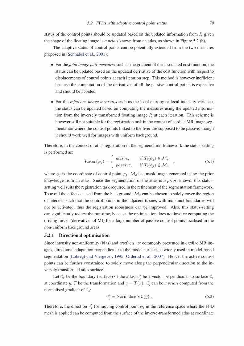
5.2. FFDs with adaptive control point status 79
status of the control points should be updated based on the updated information from I is given
the shape of the floating image is a priori known from an atlas, as shown in Figure 5.2 (b).
The adaptive status of control points can be potentially extended from the two measures
proposed in (Schnabel et al., 2001):
• For the joint image pair measures such as the gradient of the associated cost function, the
status can be updated based on the updated derivative of the cost function with respect to
displacements of control points at each iteration step. This method is however inefficient
because the computation of the derivatives of all the passive control points is expensive
and should be avoided.
• For the reference image measures such as the local entropy or local intensity variance,
the status can be updated based on computing the measures using the updated informa-
tion from the inversely transformed floating image Iis at each iteration. This scheme is
however still not suitable for the registration task in the context of cardiac MR image seg-
mentation where the control points linked to the liver are supposed to be passive, though
it should work well for images with uniform background.
Therefore, in the context of atlas registration in the segmentation framework the status-setting
is performed as:
Status(ϕj) =
{active, if Ti(φj) ∈ Ms
passive, if Ti(φj) /∈ Ms
, (5.1)
where φj is the coordinate of control point ϕj , Ms is a mask image generated using the prior
knowledge from an atlas. Since the segmentation of the atlas is a priori known, this status-
setting well suits the registration task required in the refinement of the segmentation framework.
To avoid the effects caused from the background, Ms can be chosen to solely cover the region
of interests such that the control points in the adjacent tissues with indistinct boundaries will
not be activated, thus the registration robustness can be improved. Also, this status-setting
can significantly reduce the run-time, because the optimisation does not involve computing the
driving forces (derivatives of MI) for a large number of passive control points localised in the
non-uniform background areas.
5.2.1 Directional optimisationSince intensity non-uniformity (bias) and artefacts are commonly presented in cardiac MR im-
ages, directional adaptation perpendicular to the model surfaces is widely used in model-based
segmentation (Lobregt and Viergever, 1995; Orderud et al., 2007). Hence, the active control
points can be further constrained to solely move along the perpendicular direction to the in-
versely transformed atlas surface.
Let Cs be the boundary (surface) of the atlas, �vsy be a vector perpendicular to surface Csat coordinate y, T be the transformation and y = T (x). �vsy can be a priori computed from the
normalised gradient of Cs:
�vsy = Normalise ∇C(y) . (5.2)
Therefore, the direction �vtx for moving control point φj in the reference space where the FFD
mesh is applied can be computed from the surface of the inverse-transformed atlas at coordinate

80 Chapter 5. Constrained Driving Forces in Nonrigid Registration
x = φj . Since T−1(Cs)(x) = Cs(y) and y = T (x), �vtx can be computed as:
�vtx = Normalise ∇(T−1(Cs)(x))= Normalise ∇(Cs(T (x))= Normalise
(∇Cs(y) · ∇T (x)) . (5.3)
5.3 Experiments and results5.3.1 Experiment-1: Registration using phantom data
(a) (b)
(c) (d) (e)
Figure 5.3: Images used in the experiment: (a): three views of the reference image; (b): the
floating image; the images are with simulated noise and ghosting artefacts. (c)-(e): a single
view of the three mask images (red) superimposing on the floating image, (c) 20 mm width, (d)
30 mm width, and (e) 40 mm width.
Data and experimental setupThe purpose of this experiment is to demonstrate the registration performance difference using
the standard FFDs and adaptive status FFDs, and the performance difference of the adaptive
status FFDs using different mask images Ms for the status setting. The reference and floating
images used in this experiment are shown in Figure 5.3 (a) and (b). They were constructed from
intensity uniform images with a square and a sphere. Rician noise with amplitudes of 3-5% of
the intensity ranges was added and rotational and vertically translational motions were also
simulated to the image construct to include some artefacts such as the ghosting in the images.
The images are of resolution 100× 100× 100 and of pixel size 2× 2× 2 mm.
We employed 52 random affine transformations (without translation) to transform the float-
ing image to generate 52 registration tasks. A nonrigid registration was used to register the
transformed floating images to the reference image. The accuracy of a registration result was
assessed using the surface-to-surface distance between the box in the reference image and the
transformed sphere in resultant floating image. For each case, a root mean square (RMS) sur-
face distance error measure and the computation time of registration were computed.
The nonrigid registration used two-level FFD meshes as the transformations models, a
coarse level with isotropic spacing 20 mm and a fine level with isotropic spacing 10 mm. The

5.3. Experiments and results 81
goal of the registration tasks was to align the surface of the box and the surface of the sphere,
thus the active control points in the adaptive setting scheme should be associated with the region
around the surface in the floating image. By changing the size of this region, we compared the
results of four registration schemes:
(1) Adaptive control point status FFD registration with a mask image whose thickness is
twice the FFD mesh spacing around the surface of the sphere. Figure 5.3 (c) shows the
mask of 20 mm size, twice the 10 mm spacing FFD grid, while in the level of 20 mm
spacing, the mask is 40 mm size, shown in (e). This scheme is referred to as ACPS-2.
(2) Adaptive control point status FFD registration with a mask image whose thickness is
three times the FFD mesh spacing around the surface of the sphere. Figure 5.3 (d) shows
the mask of 30 mm size, three times the 10 mm spacing FFD grid, while in the level of
20 mm spacing, the mask is 60 mm size. This scheme is referred to as ACPS-3.
(3) Adaptive control point status FFD registration with a mask image whose thickness is four
times the FFD mesh spacing around the surface of the sphere. Figure 5.3 (e) shows the
mask of 40 mm size, four times the 10 mm spacing FFD grid, while in the level of 20
mm spacing, the mask is 80 mm size. This scheme is referred to as ACPS-4.
(4) Standard FFD registration without status setting. This scheme is referred to as Full FFDs.
All the four registration schemes adopted the same gradient ascent optimisation scheme
and the stopping criterion was the registration reaching an optimum of the normalised mutual
information similarity measure. The concatenation scheme (Rueckert et al., 2006) was used to
maintain diffeomorphism.
ResultTable 5.1 presents the results of the four registration schemes. In terms of registration accuracy,
ACPS-2 performed significantly worse than the other three as their mean errors were all at least
twice their standard deviations away from the mean error of ACPS-2. However, in terms of
computation time ACPS-2 also had demonstrated a significant superiority over the other three:
its average run-time was far (more than three times its standard deviations) away from the mean
of the others. Full FFDs performed far slower as the mean run time of the other three schemes
were all more than three times their standard deviations away from the mean of Full FFDs. Also
the accuracy of Full FFDs was not significantly different from that of ACPS-3 (P = 0.16) and
ACPS-4 (P = 0.87) using the paired t-test. It should be noted that the registration results, the
RMS errors and run time in Table 5.1, were approximately considered as Gaussian distributed
when doing the comparisons using mean and standard deviation, and the t-test, based on the
same argument in Page 75, Section 4.5.4.
ConclusionIn conclusion, the performance of ACPS-3 and ACPS-4 was similar, and both were better than
ACPS-2 in terms of the registration accuracy but worse in terms of the run time. No evidence
showed that Full FFDs could achieve better registration accuracy than ACPS-3 or ACPS-4, but
the computation time was significantly longer than that of the other schemes. Therefore, in

82 Chapter 5. Constrained Driving Forces in Nonrigid Registration
Table 5.1: The registration errors (RMS surface distance) and computation time of the four
registration schemes. mm: millimeter, min: minute.
ACPS-2 ACPS-3 ACPS-4 Full FFDs
Erorr (mm) 1.54± 0.14 1.26± 0.06 1.22± 0.06 1.23± 0.12Run time (min) 8.2± 2.0 15.7± 5.1 18.2± 4.7 52.3± 12.9
cardiac MR registration, ACPS-2 and ACPS-3 are preferred because they have been shown to
be able to achieve enough accuracy for the registration needs. Also, activating fewer control
points can practically reduce the chance of registering the non-uniform background of the MR
images and improve the registration within the heart region.
5.3.2 Experiment-2: Application to whole heart segmentationData and experimental setupThe purpose of this experiment is to compare the registration performance of the proposed
ACPS FFDs and the standard FFDs when applied to the whole heart segmentation framework,
leading to two registration schemes as follows:
• LARM ACPS: A global affine registration for localisation, then the locally affine regis-
tration method (LARM) for substructure initialisation, finally the FFD registration with
adaptive control point status for refinement of the local details.
• LARM FFDs: A global affine registration for localisation, then LARM for substructure
initialisation, finally the standard FFD registration for refinement of the local details.
The experiment employed 10 pathological MR cases, which displayed a variety of heart ab-
normalities due to either Tetralogy of Fallot or myocardial infarction. The acquisition of these
images has been presented in Section 4.5.1. The manual segmentation, regarded as the gold
standard segmentation, was done by a technician with cardiac anatomy knowledge, slice by
slice using Analyze 8.1, Philips, The Netherlands. The segmentation error was computed from
the RMS surface distance between the segmented surface and the gold standard.
Table 5.2: The segmentation error, RMS surface distance, and the percentage (%) of the error
ranges: <2 mm, 2-5 mm, and >5 mm.
Method Structure RMS (mm) <2 mm (%) 2-5 mm (%) >5 mm (%)
LARM ACPS Epicardium 2.3± 0.7 75.3± 6.2 19.9± 4.2 4.8± 3.7Left Ventricle 1.6± 0.3 83.8± 7.8 14.9± 7.3 1.3± 0.9Right Ventricle 1.9± 0.6 82.2± 5.7 14.5± 4.0 3.3± 3.2Left Atrium 2.3± 0.6 71.5± 10.4 24.0± 9.0 4.5± 5.3Right Atrium 1.8± 0.4 80.6± 6.7 16.9± 5.0 2.5± 2.7Whole Heart 1.8± 0.2 81.1± 4.0 16.7± 3.9 2.2± 1.2
LARM FFDs Epicardium 3.1± 1.1 72.5± 5.9 20.2± 4.2 7.4± 5.2Left Ventricle 1.8± 0.7 81.2± 8.4 16.7± 7.1 2.1± 2.7Right Ventricle 1.9± 0.6 80.0± 7.9 16.7± 5.8 3.2± 3.1Left Atrium 2.5± 1.0 68.2± 9.9 25.0± 6.3 6.8± 7.3Right Atrium 2.2± 0.7 74.2± 7.1 21.5± 5.7 4.3± 4.0Whole Heart 2.0± 0.3 77.0± 4.2 20.3± 4.0 2.7± 1.5

5.3. Experiments and results 83
Figure 5.4: Three views, sagittal, transverse, coronal views of segmented contour superimpos-
ing on the MR images. These are four random examples of using the LARM ACPS registration
scheme (left) and the LARM FFDs scheme (right).
Result
Table 5.2 presents the segmentation errors for each anatomical structures, including epicardial
surface of the left ventricle (Epicardium), endocardial surface of the left and right ventricles
(Left Ventricle and Right Ventricle), endocardial surface of the left and right atria (Left Atrium
and Right Atrium) and all these surfaces as one measure (Whole Heart). LARM ACPS al-
most outperformed LARM FFDs in every categories, particularly, in Epicardium (P=0.04) and
Whole Heart (P=0.03) categories the segmentation accuracy was significantly different, using
0.05 as the significance level in the paired t-test. The larger errors from the standard FFDs in the
registration of epicardium was mainly due to adjacent tissues such as the liver and lung which
could affect the registration of the indistinct boundaries. For this reason, the registration was
more likely to step into local minima and produce unrealistic deformations, as the examples
shown in Figure 5.4.
Table 5.2 also gives the error ranges of each structure category. Over 80% of the seg-
mentation by LARM ACPS was within 2 mm and more than 97% within 5mm. The segmen-

84 Chapter 5. Constrained Driving Forces in Nonrigid Registration
tation errors of different substructures could be quite different, for example the Left Ventricle
(1.6± 0.3 mm) achieved much better, more than three times standard deviation, than that of the
Left Atrium (2.3± 0.6) due to the limitation of the validation scheme.
Three Gaussian distribution assumption used in the t-test and the three groups of error
distribution are based on the same arguments in Page 72 and Page 75, respectively. More
detailed studies and discussion of the segmentation performance will be given in chapter 6.
ConclusionThis experiment showed that by taking the a priori knowledge into the status-setting of the FFD
meshes, the proposed FFD registration improved the segmentation performance when applied
to the registration-based segmentation propagation framework. This segmentation achieved a
RMS surface-to-surface error of 1.8± 0.2 mm in the 10 pathological cases, considerably better
than the segmentation by using the standard FFDs, particularly in the epicardium.
5.4 ConclusionIn this chapter, we have presented a new FFD registration with adaptive control point status.
In this scheme, the control points activated for optimisation are related to the priorly selected
regions and adaptively changeable according to the current deformation field. The phantom
experiment demonstrated that the proposed method not only could achieve the high accuracy as
the standard FFDs for the registration of the region of interests, but also significantly improved
the computation time. The experiment of MR segmentation framework demonstrated a signifi-
cantly different (better) accuracy using the proposed FFDs for the refinement, compared to the
standard FFDs.

Chapter 6
Whole Heart Segmentation
This chapter describes a fully automatic whole heart segmentation framework using the two new
registration algorithms introduced in the last two chapters: the locally affine registration method
(LARM) and the free-form deformations with adaptive control point status (ACPS FFDs). Sec-
tion 6.1 gives an introduction to this work. Section 6.2 presents the segmentation framework in
detail, and Section 6.3 describes the procedure of constructing the atlas. Section 6.4 shows the
validation results and Section 6.5 concludes this chapter.
6.1 Introduction
Magnetic resonance (MR) imaging has become a routine modality for the determination of pa-
tient cardiac morphology. The extraction of this information can be important for the develop-
ment of new clinical applications as well as the planning and guidance of cardiac interventional
procedures. To avoid inter- and intra-observer variability of manual delineation, it is highly de-
sirable to develop an automatic technique for whole heart segmentation of cardiac MR images.
However, automating this process is complicated by the limited quality of acquired images and
the large shape variation of the heart between subjects.
We propose a registration framework able to preserve the topology and to deal with the
large shape variability of the heart. The core process is based on the two new algorithms: the
locally affine registration method (LARM) and the nonrigid registration algorithm using free-
form deformations with adaptive control point status (ACPS FFDs). In this scheme, LARM is
applied to obtain a robust initialisation of the different substructures of the heart such as the
four chambers and the great vessels. The resultant transformation globally deforms the atlas
but locally still maintains the shape of the substructures. This registration is able to avoid local
optima during the optimisation of the global transformation. After the initialisation, ACPS
FFD registration is used to refine the local details. The control point status-setting in ACPS
FFD registration makes advantageous use of prior knowledge to avoid the myocardial leakingproblem.
Furthermore, an inverse transformation is needed from LARM to propagate the segmenta-
tion. This is because LARM requires the local regions pre-defined in the reference image space,
while the atlas which has the definition is the floating image in the segmentation framework.
Hence, the Dynamic Resampling And distance Weighted interpolation (DRAW) method will
be used to compute the inverse transformation for LARM registration.

86 Chapter 6. Whole Heart Segmentation
6.2 Segmentation framework
(1) An unseen image needing segmentation(2) Atlas intensity image for registration(3) Atlas label image with segmentation information(4) Resultant segmentation for the unseen image
LARM
DRAW
ACPS FFDsRegistration
ResultantTransformation
Global AffineRegistrationInput
GenerateSegmentation
and
Figure 6.1: The framework of automatic whole heart segmentation based on atlas propagation.
The segmentation framework, registering the atlas to unseen images for segmentation
propagation as illustrated in Figure 6.1, includes three registration steps:
(1) Firstly, a global affine registration is applied to localize the heart. In cardiac MR seg-
mentation, localisation of the heart is an essential step for success and a challenging one
to fully automate (Peters et al., 2009; Kurkure et al., 2009). In this framework, a global
affine registration works well because of the following two reasons. Firstly, the field of
view from different scans is similar. This MRI scan covers the background structures of
the heart such as the back, chest, and the liver, which contribute to the localisation of the
heart. Secondly, the atlas and unseen images have similar orientation. The MR data have
been acquired from either short-axis or sagittal views and the rotation for compensating
the orientation difference is smaller than 90 degrees. Figure 6.2 (left) shows an example
image.
(2) LARM is then used to further initialise the substructures. Three stages of LARM reg-
istration are adopted in practice, where two, four, seven local affine transformations are
used respectively.
In the first stage, only two local affine transformations are used. The corresponding local
regions are defined as the atrial region including the two atria and the great vessels, and
the ventricular region including the two ventricles. In the second stage, the right ventricle
and the right atrium are separated from the regions defined in the first stage to add another
two affine transformations. Finally, seven local regions, including the two ventricles, the
two atria, the pulmonary artery, the ascending aorta, and the descending aorta, are used
to define a seven-local-affine LARM.
In all the three stages, the atlas image is used as a reference image in LARM. Therefore,

6.3. Atlas construction 87
DRAW is used to get the transformation field defined from the unseen MR image to the
atlas.
(3) Finally, registration using ACPS FFDs is employed to refine the local details. In the
status-setting, two mask images, M1s and M2
s, are used.
Firstly, the registration uses M1s to solely activate the control points which map onto
the blood pool of the atlas. This registration mainly contributes to the alignment of the
endocardial surfaces where the boundaries are normally distinct. Hence, M1s is only
defined to cover these regions. The FFDs use isotropic B-spline meshes with a spacing
of 20 mm.
Secondly, the registration employs M2s to activate the control points which map to a
neighbouring region of the endocardial and epicardial surfaces. This step fine-tunes the
registration of whole heart surfaces and uses finer B-spline meshes with a spacing of 10
mm.
For the implementation of registration, we use NMI (Studholme et al., 1999) as the sim-
ilarity measure. The optimisation adopts the gradient ascent method and the multiresolution
scheme (Thevenaz and Unser, 2000). The registration stops when the NMI measure has not
improved in the last five steps.
6.3 Atlas constructionAtlas construction is a different topic outside the scope of this work, especially when involving
the statistical shape modelling (Frangi et al., 2002). We propose to use a simple atlas, without
statistical shape information, for the validation of the proposed method. This is because it is
assumed that the existing statistical shape models could not perform better than a simple atlas
when applied to new pathologies. Therefore, the atlas can be built from a selected reference
space such as the mean of a group of images or a space defined by any cardiac MR case.
Furthermore, it should be noted that the proposed segmentation method would benefit a lot
more from using an atlas constructed from cardiac MR data exhibiting similar heart shapes
and pathologies to the unseen data. However, to demonstrate the applicability of the proposed
framework in the most challenging tasks, we propose to use an atlas constructed from healthy
volunteer data, which is validated by evaluating the performance of this atlas in segmenting
pathological cases.
Theoretically, one can use an MR image and its corresponding segmentation as the atlas
for propagation. However, the noise and artefacts presented in a specific case can practically
lead to segmentation bias in all the cases. To avoid this, we employ a number of MR images,
such as five or ten in the experiments in Section 6.4, acquired using the same MRI sequence.
They are then registered to a selected reference space. A mean intensity image, referred to as
atlas intensity image, can be computed from this set of registered MR images. The labelling of
each anatomical region of the reference space has the corresponding segmentation information
of the atlas, referred to as atlas label image. Figure 6.2 shows an atlas case from Section 6.4,
which is constructed from ten MR images.
To achieve the registration of this set of MR images, we manually label each anatomical
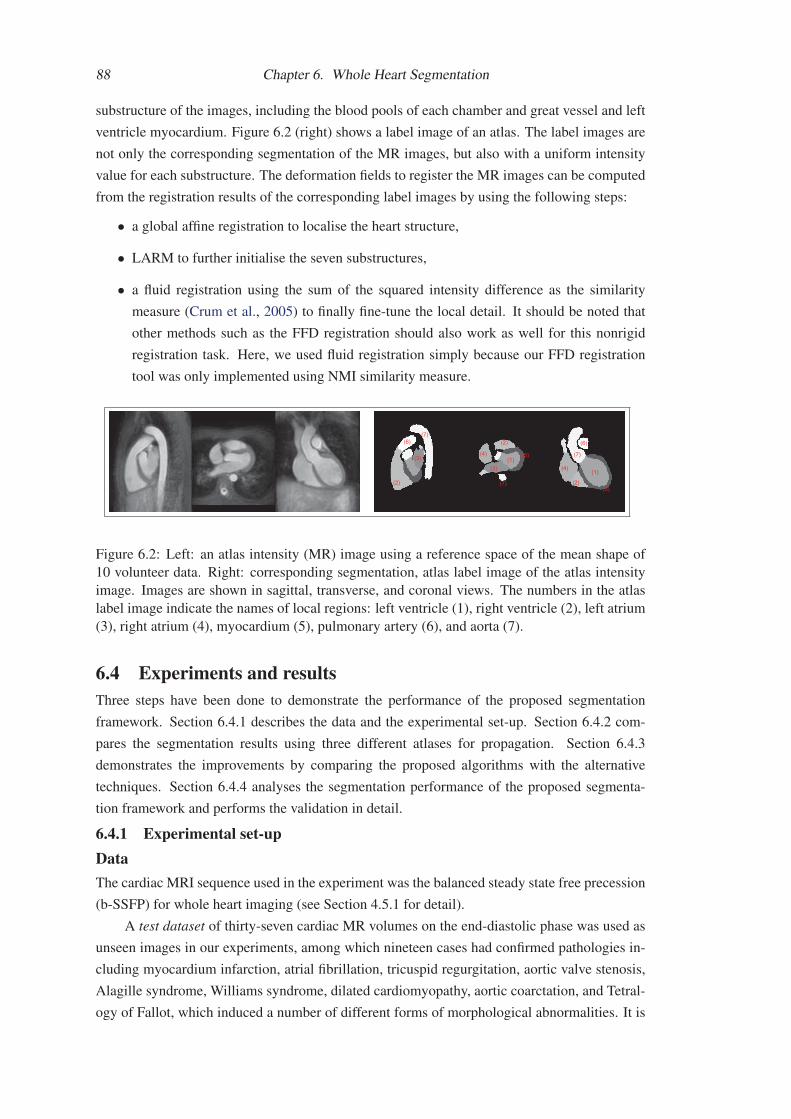
88 Chapter 6. Whole Heart Segmentation
substructure of the images, including the blood pools of each chamber and great vessel and left
ventricle myocardium. Figure 6.2 (right) shows a label image of an atlas. The label images are
not only the corresponding segmentation of the MR images, but also with a uniform intensity
value for each substructure. The deformation fields to register the MR images can be computed
from the registration results of the corresponding label images by using the following steps:
• a global affine registration to localise the heart structure,
• LARM to further initialise the seven substructures,
• a fluid registration using the sum of the squared intensity difference as the similarity
measure (Crum et al., 2005) to finally fine-tune the local detail. It should be noted that
other methods such as the FFD registration should also work as well for this nonrigid
registration task. Here, we used fluid registration simply because our FFD registration
tool was only implemented using NMI similarity measure.
(1)
(1)
(2)
(2)
(2)
(3)
(3)
(4)
(4)
(5)
(6) (6)(7)
(7)
(7)
(5)
Figure 6.2: Left: an atlas intensity (MR) image using a reference space of the mean shape of
10 volunteer data. Right: corresponding segmentation, atlas label image of the atlas intensity
image. Images are shown in sagittal, transverse, and coronal views. The numbers in the atlas
label image indicate the names of local regions: left ventricle (1), right ventricle (2), left atrium
(3), right atrium (4), myocardium (5), pulmonary artery (6), and aorta (7).
6.4 Experiments and resultsThree steps have been done to demonstrate the performance of the proposed segmentation
framework. Section 6.4.1 describes the data and the experimental set-up. Section 6.4.2 com-
pares the segmentation results using three different atlases for propagation. Section 6.4.3
demonstrates the improvements by comparing the proposed algorithms with the alternative
techniques. Section 6.4.4 analyses the segmentation performance of the proposed segmenta-
tion framework and performs the validation in detail.
6.4.1 Experimental set-upDataThe cardiac MRI sequence used in the experiment was the balanced steady state free precession
(b-SSFP) for whole heart imaging (see Section 4.5.1 for detail).
A test dataset of thirty-seven cardiac MR volumes on the end-diastolic phase was used as
unseen images in our experiments, among which nineteen cases had confirmed pathologies in-
cluding myocardium infarction, atrial fibrillation, tricuspid regurgitation, aortic valve stenosis,
Alagille syndrome, Williams syndrome, dilated cardiomyopathy, aortic coarctation, and Tetral-
ogy of Fallot, which induced a number of different forms of morphological abnormalities. It is

6.4. Experiments and results 89
common to see that many of these patients had symptoms of a combination of more than one of
these pathologies. The subjects, aged from 5 to 80, displayed a wide diversity of heart shapes.
We further acquired a training dataset from another 10 healthy volunteers for the construction
of atlases. The atlases were then used to segment the pathological data, instead of using an
atlas with a similar heart shape to unseen images, to demonstrate the general performance of
the proposed segmentation framework.
All these data have manual segmentation as the gold standard. They were either done using
a mesh model with manual corrections (Peters et al., 2007) or using the manual editing tool in
the commercial product Analyze 8.1 or 9.0, Philips, The Netherlands. The manual segmentation
was completed by either a clinician or a research associate with detailed knowledge of heart
anatomy. For the test dataset, the blood cavities of the four chambers and the myocardium
of the left ventricle are separately segmented (examples of manual segmentation can be found
in Figure 6.4 and Figure 6.5), while for the training dataset, in addition to these regions, the
pulmonary artery, ascending aorta and aortic arch, and descending aorta are also separately
delineated for the atlas construction registration. Figure 6.2 (right) shows an example of these
substructure labels.
Evaluation protocolsTwo different types of measures are used to evaluate the accuracy of a segmentation result: the
surface distance measures and the volume measures.
The surface measures compute the surface-to-surface distance between the propagated seg-
mentation and the gold standard segmentation. This surface distance is calculated using each
surface point sseg from the propagated segmentation to the triangle defined by the three closest
surface points {s1gd, s2gd, s3gd} of sseg in the gold standard segmentation. The mean surface
distance, εmean, standard deviation, εstd, and the root mean square (RMS), εrms of a surface
are computed. Six surfaces are considered:
(1) the endocardial surface of the left ventricle, referred to as Left Ventricle,
(2) the endocardial surface of the left atrium, referred to as Left Atrium,
(3) the endocardial surface of the right ventricle, referred to as Right Ventricle,
(4) the endocardial surface of the right atrium, referred to as Right Atrium,
(5) the epicardial surfaces of the left ventricles, referred to as Epicardium,
(6) the inclusion of all the five surfaces above as a whole heart segmentation accuracy, re-
ferred to as Whole Heart.
Volume measurement is of major interest in many clinical applications such as computing
stroke volume, eject fraction and myocardium mass. Three widely used measures are employed
in the validation, including:
• Dice Coefficient = 2|Vseg ∩ Vgd|/(|Vseg|+ |Vgd|) (Dice, 1945),
• Volume Overlap = |Vseg ∩ Vgd|/|Vseg ∪ Vgd| (Crum et al., 2006),

90 Chapter 6. Whole Heart Segmentation
• Volume Difference = 2×ABS(|Vseg| − |Vgd|)/(|Vgd|+ |Vseg|)× 100%,
where, Vseg and Vgd denote the volumes from the propagated segmentation and gold standard
respectively. Both Dice and volume overlap indicate how well the two volumes are overlapped,
with maximum 1 meaning perfect overlap and minimum 0 indicating no overlap at all. Five
substructures are measured, as follows:
(1) the blood cavity of left ventricle, referred to as Left Ventricle,
(2) the blood cavity of left atrium, referred to as Left Atrium,
(3) the blood cavity of right ventricle, referred to as Right Ventricle,
(4) the blood cavity of right atrium, referred to as Right Atrium,
(5) the myocardium of the left ventricle, including septum, referred to as Myocardium.
Three steps of evaluationStep-one: This step uses the 19 pathological data as a test set to assess the sensitivity of the
proposed approach to different atlases. Section 6.3 provides the detail of the atlas construction.
Three atlases are tested, whose reference spaces are based on the following:
(1) A healthy volunteer MR image is randomly selected from the training dataset as the
reference space, referred to as One Shape.
(2) The mean shape of five randomly selected training data is used as the reference space,
referred to as Five Shapes. The mean of five shapes was computed based on the iterativeatlas construction (Frangi et al., 2002). The registration in our construction employs the
five corresponding label images and the three transformation models introduced in the
atlas construction, described in Section 6.3.
(3) The mean shape of all the ten volunteer data is used as the reference space, referred to as
Ten Shapes. Figure 6.2 shows the result of this atlas.
Step-two: This step assesses the improvement of the proposed two registration algorithm-
s when applied to the segmentation framework. The atlas used is the Ten Shapes. Three reg-
istration frameworks, for the segmentation propagation, are used to segment the test set of
thirty-seven cases, including:
• a single affine for global localisation and a traditional FFDs (Rueckert et al., 2006) for
refinement, referred to as Affine FFDs,
• a single affine for global localisation, then LARM for substructure initialisation, finally
traditional FFDs for refinement, referred to as LARM FFDs,
• the proposed framework, a single affine for global localisation, then LARM for substruc-
ture initialisation, finally a registration using ACPS FFDs for refinement, referred to as
LARM ACPS.

6.4. Experiments and results 91
The FFD registration in all cases used multi-level, from isotropic 20 mm mesh spacing to 10
mm, FFD meshes (Schnabel et al., 2001) and the concatenation strategy (Rueckert et al., 2006)
to maintain diffeomorphism.
Step-three: Finally, we focus on the segmentation results of the 37 test data using the
proposed segmentation framework and theTen Shapes atlas.
Figure 6.3: The individual plots and the Box-and-Whisker diagrams of the Whole Heart seg-
mentation errors using the RMS surface-to-surface error measure, εrms. Left: the errors of the
19 pathological cases using the proposed segmentation approach combined with the three differ-
ent atlases. Right: the errors of the 37 cases using the three different segmentation frameworks.
Note that the red crosses are these considered as outliers in the box plots.
6.4.2 Sensitivity to different atlasesFigure 6.3 (left) plots the RMS surface distance errors of the 19 pathological cases. The mean
and standard deviation of the errors are:
• using One Shape atlas: 2.63± 0.70 (mm),
• using Five Shape atlas: 2.47± 0.57 (mm),
• using Ten Shape atlas: 2.47± 0.61 (mm).
Both the Box-and-Whisker diagram and figures from mean and standard deviation show
that the segmentation using the Five Shapes atlas had smaller error numbers while using the
One Shape atlas had greater numbers. However, the differences between the mean and median
numbers are all less than 0.2 mm. To assess the significance of the performance difference, the
two tailed, paired t-test (Glantz, 2005) was used: P1,5 = 0.068 (between the One Shape and
the Five Shapes), P1,10 = 0.057 (between the One Shape and the Ten Shapes), and P5,10 =
0.95 (between the Five Shapes and the Ten Shapes). There was no strong evidence showing
significant difference between each population using a significance level of 0.05. However,
both P1,5 and P1,10 were also close to the significance level. We then further computed the 0.95
confidence interval of them, which were CI1,5 = [0.01, 0.32] mm and CI1,10 = [0.01, 0.31]
mm respectively. This showed there were small biases of the One Shape population with respect
to the other two, but these biases were not practically important, as the mean errors of repeated
manual segmentation to the gold standard segmentation, in εrms, are shown to be between 0.5 to
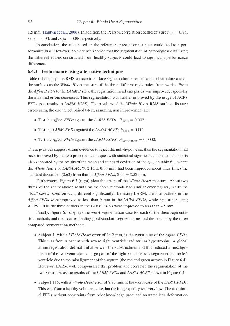
92 Chapter 6. Whole Heart Segmentation
1.5 mm (Hautvast et al., 2006). In addition, the Pearson correlation coefficients are r1,5 = 0.94,
r1,10 = 0.93, and r5,10 = 0.98 respectively.
In conclusion, the atlas based on the reference space of one subject could lead to a per-
formance bias. However, no evidence showed that the segmentation of pathological data using
the different atlases constructed from healthy subjects could lead to significant performance
difference.
6.4.3 Performance using alternative techniquesTable 6.1 displays the RMS surface-to-surface segmentation errors of each substructure and all
the surfaces as the Whole Heart measure of the three different registration frameworks. From
the Affine FFDs to the LARM FFDs, the registration in all categories was improved, especially
the maximal errors decreased. This segmentation was further improved by the usage of ACPS
FFDs (see results in LARM ACPS). The p-values of the Whole Heart RMS surface distance
errors using the one tailed, paired t-test, assuming non improvement are:
• Test the Affine FFDs against the LARM FFDs: Plarm = 0.002.
• Test the LARM FFDs against the LARM ACPS: Pacps = 0.002.
• Test the Affine FFDs against the LARM ACPS: Plarm+acps = 0.0002.
These p-values suggest strong evidence to reject the null-hypothesis, thus the segmentation had
been improved by the two proposed techniques with statistical significance. This conclusion is
also supported by the results of the mean and standard deviation of the εrms in table 6.1, where
the Whole Heart of LARM ACPS, 2.14 ± 0.63 mm, had been improved about three times the
standard deviations (0.63) from that of Affine FFDs, 3.96± 3.23 mm.
Furthermore, Figure 6.3 (right) plots the errors of the Whole Heart measure. About two
thirds of the segmentation results by the three methods had similar error figures, while the
“bad” cases, based on εrms, differed significantly: By using LARM, the four outliers in the
Affine FFDs were improved to less than 9 mm in the LARM FFDs, while by further using
ACPS FFDs, the three outliers in the LARM FFDs were improved to less than 4.5 mm.
Finally, Figure 6.4 displays the worst segmentation case for each of the three segmenta-
tion methods and their corresponding gold standard segmentations and the results by the three
compared segmentation methods:
• Subject-1, with a Whole Heart error of 14.2 mm, is the worst case of the Affine FFDs.
This was from a patient with severe right ventricle and atrium hypertrophy. A global
affine registration did not initialise well the substructures and this induced a misalign-
ment of the two ventricles: a large part of the right ventricle was segmented as the left
ventricle due to the misalignment of the septum (the red and green arrows in Figure 6.4).
However, LARM well compensated this problem and corrected the segmentation of the
two ventricles as the results of the LARM FFDs and LARM ACPS shown in Figure 6.4.
• Subject-116, with a Whole Heart error of 8.93 mm, is the worst case of the LARM FFDs.
This was from a healthy volunteer case, but the image quality was very low. The tradition-
al FFDs without constraints from prior knowledge produced an unrealistic deformation

6.4. Experiments and results 93
Subject-1, gold standard segmentation Subject-1, LARM ACPS segmentation
Subject-1, LARM FFDs segmentation Subject-1, Affine FFDs segmentation
Subject-116, gold standard segmentation Subject-116, LARM ACPS segmentation
Subject-116, LARM FFDs segmentation Subject-116, Affine FFDs segmentation
Subject-9, gold standard segmentation Subject-9, LARM ACPS segmentation
Subject-9, LARM FFDs segmentation Subject-9, Affine FFDs segmentation
Figure 6.4: The worst cases by the three segmentation methods. Subject-1 is the worst case
of the Affine FFDs, subject-116 is the worst case of LARM FFDs, and subject-9 is the worst
case of LARM ACPS. Images are displayed with delineated contour superimposed on the MR
images, in sagittal, transverse, and coronal views. Subject-1 and subject-9 are pathological
cases while subject-116 is a healthy case.

94 Chapter 6. Whole Heart Segmentation
Table 6.1: Surface-to-surface segmentation errors in millimeters, εrms of the three methods and
errors εmean, εstd, and percentage with different ranges: < 2 mm, 2 − 5 mm, and > 5 mm, of
the 37 cases by the proposed approach.(error in mm) Affine FFDs LARM FFDs LARM ACPS in different measures (ranges are of unit mm)
Structures εrms[max] εrms[max] εrms[max] εmean εstd 0− 2 2− 5 > 5Left Ventricle 3.79± 4.38[19.6] 1.89± 1.10[7.12] 1.47± 0.32 [2.38] 1.06 1.02 82.9% 16.5% 0.6%
Left Atrium 3.26± 2.25[11.5] 2.81± 1.65[9.28] 2.38± 1.14 [7.33] 1.69 1.68 70.2% 23.5% 6.4%
Right Ventricle 3.23± 1.79[7.50] 2.75± 1.51[8.57] 2.13± 0.70 [4.05] 1.50 1.51 72.2% 24.1% 3.7%
Right Atrium 3.06± 1.74[9.44] 2.51± 1.20[7.05] 2.22± 0.75 [5.74] 1.51 1.62 73.0% 22.5% 4.5%
Epicardium 4.78± 4.88[20.4] 2.88± 2.12[12.9] 2.32± 0.82 [5.43] 1.69 1.60 68.6% 25.7% 5.6%
Whole Heart 3.96± 3.23[14.2] 2.71± 1.50[8.93] 2.14± 0.63 [4.31] 1.47 1.55 73.6% 22.5% 3.9%
field and resulted in an erroneous result, while ACPS FFD registration contributed to
reduce this error.
• Subject-9, with a Whole Heart error of 4.31 mm, is the worst case of the LARM ACPS.
This case was also the worst result of the LARM ACPS in terms of the error measure for
the left atrium (7.33 mm), right ventricle (4.05 mm), and right atrium (5.74 mm). The
large error for the right ventricle was mainly due to the inconsistent delineation of the cut-
ting boundaries of chordae tendineae, papillary muscle, and trabeculae carnae (indicated
by the red arrows in Figure 6.4) between the gold standard and propagated segmentations.
The error for the atria was attributed to the fact that the propagated segmentation included
parts of adjacent veins into the volume of atria, especially the left atrium; by contrast, the
gold standard segmentation did not include them.
6.4.4 Performance of the proposed framework
Subject-119, GD Subject-119, PS Subject-43, GD Subject-43, PS Subject-10, GD Subject-10, PS
Figure 6.5: Three segmentation cases. Images are displayed with delineated contour superim-
posing on the MR images, in four-chamber (top) and short-axis (bottom) views. Subject-119 is
a healthy case while subject-10 and subject-43 are pathological cases. The Whole Heart seg-
mentation errors of them in εrms measure are 2.39 mm, 3.17 mm, and 2.86 mm respectively.
GD: gold standard segmentation; PS: propagated segmentation.
Table 6.1 lists the surface-to-surface errors of the proposed segmentation method for each
surface category. The RMS error (and its maximum over the 37 cases), the mean error, the
standard deviation, and the percentage of error ranges are presented. For an average whole
heart segmentation, more than 95% surface-to-surface error is within 5 mm.

6.4. Experiments and results 95
Figure 6.6: The individual plots and the Box-and-Whisker diagrams of the RMS surface dis-
tance measure, εrms, segmentation errors using the proposed segmentation method. This figure
gives the errors of each substructures as well as the Whole Heart from the 37 cases.
Figure 6.6 plots all the errors and Box-and-Whisker diagrams of the 37 cases. It agrees
with the results in table 6.1 that the segmentation of the Left Ventricle was better than other
surface categories. The worst case for the Left Ventricle was subject-119, from a healthy volun-
teer, with a RMS surface error of 2.38 mm; the worst case of the Epicardium was subject-43,
from a Tetralogy of Fallot patient, with a RMS surface error of 5.43 mm. The segmentation by
the proposed method and the gold standard segmentation are shown in Figure 6.5. The worst
segmentation of other surface categories was from subject-9, shown in Figure 6.4.
Finally, Figure 6.7 shows the colour map of surface-to-surface errors of the whole heart
segmentation. One can realise from this map that the large errors were mainly distributed to the
area of connections between substructures. For example, the area between the right ventricle
and pulmonary artery was one of the worst regions. Similar situation was found in the areas
between the left atrium and pulmonary veins and left auricula. The proposed method also had a
moderate error range in a small part of the endocardium of the right ventricle. This was because
there were many pathological cases which exhibited a thickened right ventricle myocardium,
while the atlas image did not include such myocardium. The segmentation therefore could
incorrectly segment part of the myocardium into the right ventricle blood cavity due to this
ambiguity. Examples of this error can be found in cases of subject-1 and subject-9 in Figure 6.4.
Table 6.2 presents the mean segmentation errors and their worst cases in volume measures.
This table also gives measures calculated based on all substructures in the column All substruc-tures. The worst cases for each substructure using the Dice measure were subject-116 (LeftVentricle), subject-9 (Left Atrium), subject-10 (Right Ventricle and Right Atrium), and subject-
43 (Myocardium). The segmentation of subject-116 and subject-9 are displayed in Figure 6.4
and that of subject-10 and subject-43 are shown in Figure 6.5.

96 Chapter 6. Whole Heart Segmentation
Figure 6.7: Two views showing the error map of surface-to-surface distance for the whole
heart segmentation by the proposed method. (Please refer to the web version of this article for
interpretation of the color map. A movie showing the color map from other angles can also be
found at http://www.cs.ucl.ac.uk/staff/X.Zhuang/.)
Table 6.2: Segmentation errors by the proposed method using volume measures: Dice coef-
ficient, volume overlap, percentage of volume difference (Diff), p-value and 0.95 confidence
interval (CI) of the difference of the segmentation errors, unit mL, and Pearson correlation R.
Structures Dice[min] Overlap[min] Diff(%)[max] P-value (CI mL) Pearson R
Left Ventricle 0.92± 0.02[0.87] 0.85± 0.04[0.78] 6.5± 4.9[19.0] 0.028 (0.5,7.5) 0.942
Left Atrium 0.81± 0.10[0.47] 0.69± 0.12[0.30] 14.1± 12.0[48.4] 0.667 (-2.7,4.2) 0.861
Right Ventricle 0.87± 0.04[0.77] 0.77± 0.06[0.63] 7.5± 4.9[19.7] 0.048 (0.1,12.3) 0.977
Right Atrium 0.84± 0.05[0.71] 0.73± 0.07[0.55] 9.0± 7.2[28.7] 0.217 (-6.8,1.6) 0.965
Myocardium 0.77± 0.06[0.52] 0.63± 0.07[0.35] 8.6± 6.9[26.7] 0.940 (-4.7,5.1) 0.892
All substructures 0.84± 0.08[0.47] 0.73± 0.10[0.30] 10.0± 9.6[48.4] 0.097 (-0.3,3.7) 0.974
From Table 6.2, we can see that there was no significant difference between the volumes
of the gold standard and the propagated segmentation for the Left Atrium (P = 0.667), the
Right Atrium (P = 0.217), the Myocardium (P = 0.940), and the All substructures volume
(P = 0.097). However, the difference was found for the Left Ventricle (P = 0.028) and the
Right Ventricle (P = 0.048). This was due to biases of the segmented volumes, shown in their
confidence intervals. Figure 6.8 shows the Bland-Altman plots of the volumes, which confirms
that both the Left Ventricle and the Right Ventricle had segmentation biases of 4.3 mL and 6.2
mL respectively. The larger bias of Right Ventricle were partly due to the inconsistent definition
of the valves between the gold standard and the propagated segmentation, as the Right Atriumhad -2.6 mL segmentation bias. Considering the ranges of their volumes were 67-204 mL and
65-488 mL, these biases should be practically unimportant. The bias for the segmentation of
all substructures was 1.70 mL. Finally, their Pearson correlation coefficients are also given in
table 6.2.
Figure 6.9 plots Bland-Altman and linear regression for the segmentation of all substruc-
tures. The proposed segmentation framework produced a mean bias of 1.7008 mL, which was

6.4. Experiments and results 97
60 80 100 120 140 160 180 200 220-30
-20
-10
0
10
20
30Left ventricle
Mean of two measures (cm3)
Diff
eren
ce b
etw
een
two
mea
sure
s (c
m3 )
(mL)
Left Ventricle
(mL)0 20 40 60 80 100
-30
-20
-10
0
10
20
30Left atrium
Mean of two measures (cm3)
Diff
eren
ce b
etw
een
two
mea
sure
s (c
m3 )
Left Atrium
(mL)
(mL)
0 100 200 300 400 500-40
-20
0
20
40
60
80Right ventricle
Mean of two measures (cm3)
Diff
eren
ce b
etw
een
two
mea
sure
s (c
m3 )
Right Ventricle
(mL)
(mL)
0 50 100 150 200 250 300-60
-50
-40
-30
-20
-10
0
10
20
30Right atrium
Mean of two measures (cm3)
Diff
eren
ce b
etw
een
two
mea
sure
s (c
m3 )
Right Atrium
(mL)
(mL)
50 100 150 200-40
-30
-20
-10
0
10
20
30Myocardium of left ventricle
Mean of two measures (cm3)
Diff
eren
ce b
etw
een
two
mea
sure
s (c
m3 )
Myocardium
(mL)
(mL)
200 400 600 800 1000 1200-100
-80
-60
-40
-20
0
20
40
60
80
100Whole heart volume
Mean of two measures (cm3)
Diff
eren
ce b
etw
een
two
mea
sure
s (c
m3 )
Whole Heart volume
(mL)
(mL)
Figure 6.8: Bland-Altman plots of the segmented volumes using the proposed method and the
gold standard segmentation volumes, for the blood cavities of the left ventricle, the left atrium,
the right ventricle, and the right atrium, the volume of the left ventricle myocardium, and the
whole heart volume including all these substrucutres. Middle line is the bias (mean), upper and
lower lines are the 2 standard deviations.

98 Chapter 6. Whole Heart Segmentation
Figure 6.9: Bland-Altman plot (top) and linear regression plot (bottom) of all segmented vol-
umes using the proposed method and the gold standard segmentation volumes.
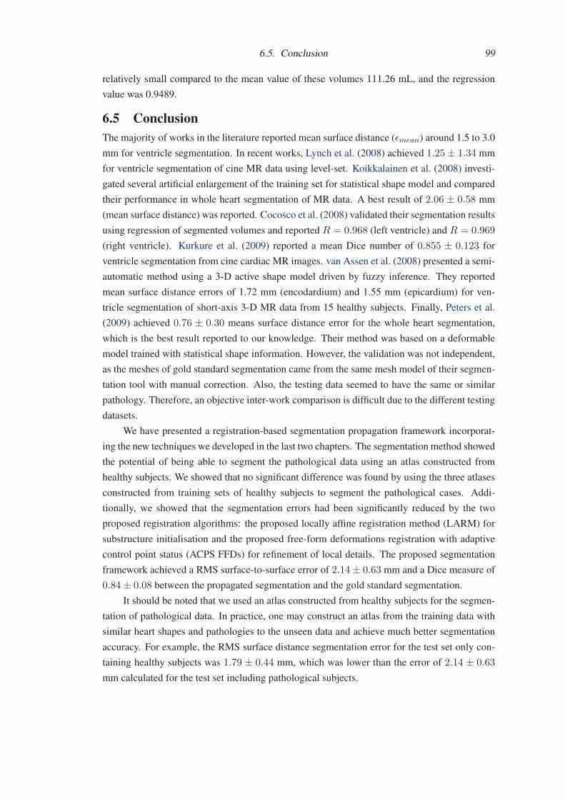
6.5. Conclusion 99
relatively small compared to the mean value of these volumes 111.26 mL, and the regression
value was 0.9489.
6.5 ConclusionThe majority of works in the literature reported mean surface distance (εmean) around 1.5 to 3.0
mm for ventricle segmentation. In recent works, Lynch et al. (2008) achieved 1.25± 1.34 mm
for ventricle segmentation of cine MR data using level-set. Koikkalainen et al. (2008) investi-
gated several artificial enlargement of the training set for statistical shape model and compared
their performance in whole heart segmentation of MR data. A best result of 2.06 ± 0.58 mm
(mean surface distance) was reported. Cocosco et al. (2008) validated their segmentation results
using regression of segmented volumes and reported R = 0.968 (left ventricle) and R = 0.969
(right ventricle). Kurkure et al. (2009) reported a mean Dice number of 0.855 ± 0.123 for
ventricle segmentation from cine cardiac MR images. van Assen et al. (2008) presented a semi-
automatic method using a 3-D active shape model driven by fuzzy inference. They reported
mean surface distance errors of 1.72 mm (encodardium) and 1.55 mm (epicardium) for ven-
tricle segmentation of short-axis 3-D MR data from 15 healthy subjects. Finally, Peters et al.
(2009) achieved 0.76 ± 0.30 means surface distance error for the whole heart segmentation,
which is the best result reported to our knowledge. Their method was based on a deformable
model trained with statistical shape information. However, the validation was not independent,
as the meshes of gold standard segmentation came from the same mesh model of their segmen-
tation tool with manual correction. Also, the testing data seemed to have the same or similar
pathology. Therefore, an objective inter-work comparison is difficult due to the different testing
datasets.
We have presented a registration-based segmentation propagation framework incorporat-
ing the new techniques we developed in the last two chapters. The segmentation method showed
the potential of being able to segment the pathological data using an atlas constructed from
healthy subjects. We showed that no significant difference was found by using the three atlases
constructed from training sets of healthy subjects to segment the pathological cases. Addi-
tionally, we showed that the segmentation errors had been significantly reduced by the two
proposed registration algorithms: the proposed locally affine registration method (LARM) for
substructure initialisation and the proposed free-form deformations registration with adaptive
control point status (ACPS FFDs) for refinement of local details. The proposed segmentation
framework achieved a RMS surface-to-surface error of 2.14± 0.63 mm and a Dice measure of
0.84± 0.08 between the propagated segmentation and the gold standard segmentation.
It should be noted that we used an atlas constructed from healthy subjects for the segmen-
tation of pathological data. In practice, one may construct an atlas from the training data with
similar heart shapes and pathologies to the unseen data and achieve much better segmentation
accuracy. For example, the RMS surface distance segmentation error for the test set only con-
taining healthy subjects was 1.79 ± 0.44 mm, which was lower than the error of 2.14 ± 0.63
mm calculated for the test set including pathological subjects.
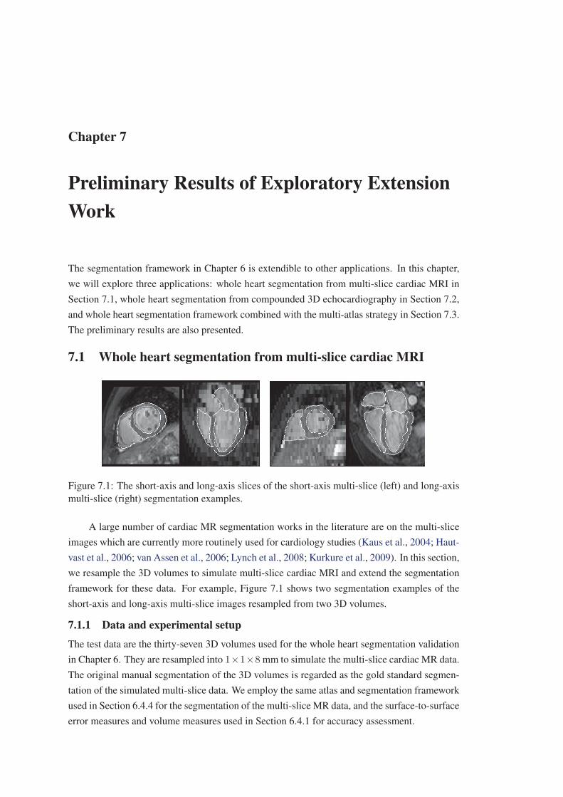
Chapter 7
Preliminary Results of Exploratory ExtensionWork
The segmentation framework in Chapter 6 is extendible to other applications. In this chapter,
we will explore three applications: whole heart segmentation from multi-slice cardiac MRI in
Section 7.1, whole heart segmentation from compounded 3D echocardiography in Section 7.2,
and whole heart segmentation framework combined with the multi-atlas strategy in Section 7.3.
The preliminary results are also presented.
7.1 Whole heart segmentation from multi-slice cardiac MRI
Figure 7.1: The short-axis and long-axis slices of the short-axis multi-slice (left) and long-axis
multi-slice (right) segmentation examples.
A large number of cardiac MR segmentation works in the literature are on the multi-slice
images which are currently more routinely used for cardiology studies (Kaus et al., 2004; Haut-
vast et al., 2006; van Assen et al., 2006; Lynch et al., 2008; Kurkure et al., 2009). In this section,
we resample the 3D volumes to simulate multi-slice cardiac MRI and extend the segmentation
framework for these data. For example, Figure 7.1 shows two segmentation examples of the
short-axis and long-axis multi-slice images resampled from two 3D volumes.
7.1.1 Data and experimental setup
The test data are the thirty-seven 3D volumes used for the whole heart segmentation validation
in Chapter 6. They are resampled into 1×1×8 mm to simulate the multi-slice cardiac MR data.
The original manual segmentation of the 3D volumes is regarded as the gold standard segmen-
tation of the simulated multi-slice data. We employ the same atlas and segmentation framework
used in Section 6.4.4 for the segmentation of the multi-slice MR data, and the surface-to-surface
error measures and volume measures used in Section 6.4.1 for accuracy assessment.

7.1. Whole heart segmentation from multi-slice cardiac MRI 101
It should be noted that the simulated images may not be representative of real clinical data.
For example, clinical data are normally used for the assessment of the ventricle and ventricular
function, and hence the coverage is limited to the ventricles only. Also, many clinical protocols
use multi-chunk, breath-hold imaging where the surfaces between slices have poorer continuity
than the simulated data. However, the image quality of multi-slice imaging provides better
image quality within slices, in particular, higher signal to noise ratio and contrast to noise ratio.
The initialisation of ventricle is also easier as all the images and template atlas can be truncated
to the short-axis ventricle regions. Therefore, we could expect better results from the validation
using an atlas constructed from real clinical data and the test set of real clinical data.
7.1.2 Results and discussion
Table 7.1: Surface-to-surface segmentation errors, εrms, εmean, εstd, and the volume measures,
Dice coefficient, volume overlap, percentage of volume difference (Diff), and Pearson correla-
tion of the 37 cases,. Whole Heart in volume measures means All Substructures.Structures εrms (mm) εmean εstd Dice Overlap Diff (%) Pearson
Left Ventricle 1.60± 0.31 1.15 1.11 0.91± 0.02 0.84± 0.04 7.2± 5.3 0.933
Left Atrium 2.68± 1.26 1.91 1.88 0.79± 0.12 0.67± 0.13 19.8± 20.3 0.831
Right Ventricle 2.22± 0.69 1.56 1.57 0.86± 0.04 0.76± 0.06 8.6± 6.6 0.974
Right Atrium 2.75± 1.27 1.89 1.99 0.81± 0.06 0.69± 0.08 11.5± 8.3 0.937
Epicardium 2.57± 0.87 1.86 1.77 0.75± 0.06 0.61± 0.07 10.4± 8.7 0.874
Whole Heart 2.39± 0.73 1.63 1.74 0.82± 0.05 0.71± 0.06 11.5± 6.7 0.967
Figure 7.2: The individual plots and the Box-and-Whisker diagrams of the segmentation errors
using the RMS surface distance measure, εrms. This figure gives the errors of each substructures
as well as the Whole Heart from the 37 simulated multi-slice cases.
Table 7.1 provides the three surface-to-surface errors measures and the volume measures
of the propagation results against the standard segmentations. The results are promising, par-
ticularly, the segmentation of ventricles which are the main interest of applications using multi-
slice MRI. Figure 7.2 plots the errors (εrms) and Box-and-Whisker diagrams of the 37 cases
in each substructures as well as the Whole Heart. Notice that the corresponding numbers and

102 Chapter 7. Preliminary Results of Exploratory Extension Work
figure of the segmentation of the original 3D volumes are presented in Table 6.1 and 6.2, and
Figure 6.6. The segmentation of multi-slice images is not as good as that of the original 3D
volumes. The Whole Heart errors, εrms, are significantly different (P < 0.001, and the 0.95
confidence interval is [0.1519, 0.3454] mm). However, the robustness of the segmentation on
the two data sets is similar as the maximal errors (4.31 versus 4.33 mm) and standard devia-
tions (0.63 versus 0.73 mm) of their Whole Heart εrms errors are similar. The difference of
segmentation accuracy is probably due to the poor resolution of the simulated multi-slice data
between slices (8mm). Particularly, this poor resolution results in larger difference of the atria
and myocardium segmentation where the volume sizes of the structures are relatively smaller.
7.2 Whole heart segmentation from compounded 3D echocardiog-raphy
7.2.1 Motivation
Ultrasound (US) imaging is a safe, low-cost, portable, and real-time interactive imaging tech-
nique, providing anatomical and diagnostic information for functional analysis. Three dimen-
sional (3D) cardiac ultrasound, also known as echocardiography or echo by cardiologists, has
the potential of providing more accurate quantitative analysis. However, most methods require
some form of segmentation process, which can be difficult to automate due to the typically low
signal-to-noise and small fields of view in US imaging.
Several papers have reported successful attempts at US segmentation in the literature (see
survey from Noble and Boukerroui (2006)). Most of the reported segmentation algorithms use
deformable models or contour models to search for optimal boundaries, with prior constraints to
maintain an anatomically realistic shape of the segmented regions. These methods have either
limited robustness or automation, similar to the problems which arise when they are applied
to cardiac MRI as we discussed in Section 3.1. By contrast, no work has been published, to
the best of our knowledge, on employing image registration techniques to perform atlas and
segmentation propagation on US images. This is probably due to the difficulty of achieving a
successful nonrigid registration using echo images. Furthermore, the current reported works
mainly focused on the left ventricle or myocardium (Mitchell et al., 2002; Orderud et al., 2007;
Zhu et al., 2007, 2009; Rajpoot et al., 2009a) due to the limited field of view of the acoustic
window from US imaging. Whole heart segmentation, unlike the ventricle segmentation, can
however provide more useful information for cardiology such as whole heart functional anal-
ysis, computational modelling, and guidance of interventional procedures. This whole heart
anatomical information is mainly available from MRI or CT. It is anticipated if this information
can also be extracted from US images, since it is the most commonly used modality for cardiac
diagnosis. This segmentation also provides an important alternative choice for cardiologists
when MRI and CT are not available or not appropriate for some patients.
Recently, compounding techniques have been shown to produce 3D echo images with a
much wider field of view and better image quality than that from a single US scan (Grau and
Noble, 2005; Grau et al., 2007; Yao et al., 2009; Rajpoot et al., 2009b). These compounded
images are created by aligning and then combining the intensity information from multiple US
image volumes. Figure 7.3 shows the example of two single-scan images and a compounded

7.2. Whole heart segmentation from compounded 3D echocardiography 103
(a) (b) (c) (d)
Figure 7.3: Example images and outputs from algorithms used during segmentation process, (a)
view from apical scan; (b) view from parasternal view; (c) compounded image from 12 scans;
(d) corresponding segmentation labels of (c).
image. The extended field of view has the potential of having whole heart coverage to carry out
the whole heart segmentation, and the combined intensity information can significantly reduce
intensity variations of tissues and boundaries presented in single-scan US images. The resultant
images hence have more consistent intensity distributions between the atlas and the US images
to be segmented. This consistency of intensity distributions enables the registration algorithms
to use intensity information for the atlas propagation-based segmentation framework.
Furthermore, the local phase analysis of US images provides a continuous scalar value
to describe the feature presented in the image. Hence, intensity-based registration can also
be applied to US images by considering the local phase value as feature intensity (Mellor and
Brady, 2005; Zhang et al., 2007). Also, a similarity measure computed from local geometrical
information such as normal vector of image intensity, also referred to as normalised gradient,
was argued to be applicable to images with different intensity distributions (Zhuang et al., 2005;
Haber and Modersitzki, 2006). This local geometrical information is based on observation
of image structures and hence applicable to US images. Therefore, we propose to use more
information from the compounded echo images for the computation of the similarity measure,
including intensity information, local phase information, and local geometrical information.
Finally, it has been shown that the registration-based segmentation propagation framework
can achieve a successful application in cardiac MR images in chapter 6. One main advantage of
this segmentation framework is that it does not require a training phase from a large dataset for
different pathologies, unlike the segmentation using statistical prior knowledge. Instead, it only
needs the prior segmentation of the template image, the atlas, to perform the propagation. This
framework is potentially applicable to a wide range of pathologies owing to the substructure
initialisation provided by the locally affine registration method (LARM). This segmentation
framework also has the potential of being applicable to other modalities including US imaging
given a similarity measure for echo registration is achievable.
7.2.2 Method
7.2.2.1 Echo and echo compounding
The echo system includes a 2D matrix array transducer X3-1 on Philips iE33 system, Philips,
the Netherlands. The acquisition has an opening angle of roughly 80 degrees and a maximal
penetration depth between 15 and 18 cm.
Compounding US images can have three potential advantages:
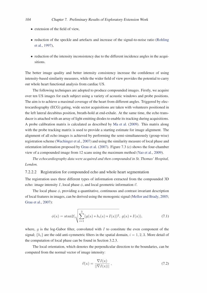
104 Chapter 7. Preliminary Results of Exploratory Extension Work
• extension of the field of view,
• reduction of the speckle and artefacts and increase of the signal-to-noise ratio (Rohling
et al., 1997),
• reduction of the intensity inconsistency due to the different incidence angles in the acqui-
sitions.
The better image quality and better intensity consistency increase the confidence of using
intensity-based similarity measures, while the wider field of view provides the potential to carry
out whole heart functional analysis from cardiac US.
The following techniques are adopted to produce compounded images. Firstly, we acquire
over ten US images for each subject using a variety of acoustic windows and probe positions.
The aim is to achieve a maximal coverage of the heart from different angles. Triggered by elec-
trocardiography (ECG) gating, wide sector acquisitions are taken with volunteers positioned in
the left lateral decubitus position, breath-hold at end-exhale. At the same time, the echo trans-
ducer is attached with an array of light emitting diodes to enable its tracking during acquisitions.
A probe calibration matrix is calculated as described by Ma et al. (2009). This matrix along
with the probe tracking matrix is used to provide a starting estimate for image alignment. The
alignment of all echo images is achieved by performing the semi-simultaneously (group-wise)
registration scheme (Wachinger et al., 2007) and using the similarity measure of local phase and
orientation information proposed by Grau et al. (2007). Figure 7.3 (c) shows the four-chamber
view of a compounded image from 12 scans using the maximum method (Yao et al., 2009).
The echocardiography data were acquired and then compounded in St. Thomas’ Hospital,London.
7.2.2.2 Registration for compounded echo and whole heart segmentation
The registration uses three different types of information extracted from the compounded 3D
echo: image intensity I , local phase φ, and local geometric information �v.
The local phase φ, providing a quantitative, continuous and contrast invariant description
of local features in images, can be derived using the monogenic signal (Mellor and Brady, 2005;
Grau et al., 2007):
φ(x) = atan2(
√√√√ 3∑i=1
(g(x) ∗ hi(x) ∗ I(x))2, g(x) ∗ I(x)), (7.1)
where, g is the log-Gabor filter, convoluted with I to constitute the even component of the
signal; {hi} are the odd anti-symmetric filters in the spatial domain, i = 1, 2, 3. More detail of
the computation of local phase can be found in Section 3.2.3.
The local orientation, which denotes the perpendicular direction to the boundaries, can be
computed from the normal vector of image intensity:
�v(x) =∇I(x)
||∇I(x)|| , (7.2)

7.2. Whole heart segmentation from compounded 3D echocardiography 105
or the normal vector of local phase
�v(x) =∇φ(x)
||∇φ(x)|| , (7.3)
since both intensity and local phase should present the same geometrical information of the
image.
Combining intensity, local phase and local geometric information, we propose the follow-
ing metric for the similarity measure of target image It and source image Is:
C = wcNCC(It, Is) + wfNCC(φt, φs) + wv1
|Ω|∫x∈Ω
[�vt(x) · �vs(x)] , (7.4)
where Ω is the image volume, NCC(It, Is) and NCC(φt, φs) are the normalised cross correlation
(NCC) of the image intensity and phase; wc, wf , and wv control the weight given to each terms.
For registration of cardiac images, we have proposed to use LARM registration to initialise
the anatomical substructures between the atlas and the unseen image. LARM defines the local
affine transformations based on the anatomical substructures of the heart, and it can preserve
the local shape of substructures and provide a robust registration for the following nonrigid
registration.
Therefore, we also adopt the locally affine transformation model for the substructure ini-
tialisation registration here. The segmentation propagation hence includes the following three
steps:
• affine registration to localise the heart structure,
• LARM to further initialise the anatomical substructures, using four local affine transfor-
mations associated with the blood cavities of the four chambers,
• free-form deformation (FFD) registration (Rueckert et al., 2006) to refine the registration
of the local details.
Gradient ascent optimisation is used for the three image registration processes. In LARM
and FFD registrations, the local phase is not transformation invariant, and so updating local
phase is computationally expensive. Therefore, we only re-estimate the local phase after every
few iteration steps, typically 10 steps to ensure that errors do not accumulate.
7.2.3 ExperimentData and experimental setup: To construct gold standard segmentation for validation, we
acquired a 3D isotropic MR image at the end-diastolic cardiac phase (same phase as used for
the compounded echo images) for each subject before acquiring the echo images. An automatic
whole heart segmentation of the MR image was then achieved using the segmentation method
we developed in Chapter 6 where a mean accuracy of 9.1% volume difference was reported for
the segmentation of the four chambers. This segmentation of the MR image was then assumed
to be the gold standard segmentation of the corresponding 3D echo with a rigid transformation
from the MR image to the echo image. The rigid transformation was obtained using a feature-
based registration algorithm (Ma et al., 2009). The registrations were also visually inspected,

106 Chapter 7. Preliminary Results of Exploratory Extension Work
Figure 7.4: Manual correction to construct the gold standard of a compounded 3D echo. Top-
left: short-axis view; top-right: two-chamber view; bottom-left: four-chamber view; bottom-
right: orthogonal planes.
and small manual corrections were carried out if errors were observed. Figure 7.4 demonstrates
an example of manual inspection. It should be noted that independent segmentations from MR
and echo images may not perfectly match (Takuma et al., 2001). This is because the different
acquisition positions from MRI (supine) and echo (left lateral decubitus) cause some deforma-
tion to the heart, in particular for the aorta. However, this difference in the four chambers, to be
validated in this study, is practically negligible compared to the segmentation errors.
Twelve propagation cases were evaluated using four sets of echo and MR data and a val-
idation strategy as follows: A dataset was chosen to represent the atlas, which was comprised
of the compounded 3D echo and the label image produced by segmenting the MR volume, an
example is shown in Figure 7.3 (c) and (d). This atlas was then propagated to segment the other
three datasets. The above was repeated four times, taking a different dataset to represent the
atlas each time. Segmentation results were assessed by comparison with the MR-derived gold
standard using the volume difference measure,
VD =2(|Vseg − Vgd|)Vseg + Vgd
× 100%, (7.5)
where Vseg is the resultant segmentation, while Vgd is the gold standard. The volume measure
was performed on the blood pools of the four chambers and the left ventricle myocardium. The
average volume of the five regions was also computed, referred to as Whole Heart.
Result and discussion: Table 7.2 gives the mean segmentation accuracy of the twelve cases,
while Figure 7.5 illustrates the visual results of four segmentation cases. The performance of the
segmentation algorithm is promising; in particular, the algorithm achieved success in the four-
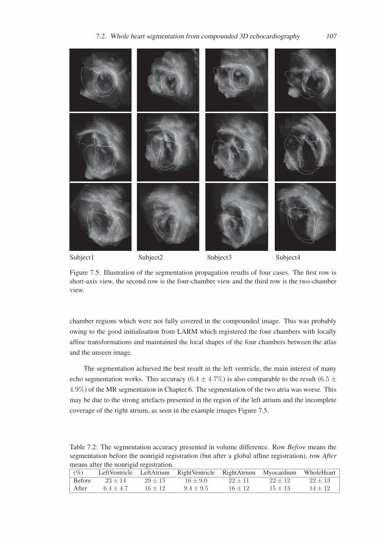
7.2. Whole heart segmentation from compounded 3D echocardiography 107
Subject1 Subject2 Subject3 Subject4
Figure 7.5: Illustration of the segmentation propagation results of four cases. The first row is
short-axis view, the second row is the four-chamber view and the third row is the two-chamber
view.
chamber regions which were not fully covered in the compounded image. This was probably
owing to the good initialisation from LARM which registered the four chambers with locally
affine transformations and maintained the local shapes of the four chambers between the atlas
and the unseen image.
The segmentation achieved the best result in the left ventricle, the main interest of many
echo segmentation works. This accuracy (6.4 ± 4.7%) is also comparable to the result (6.5 ±4.9%) of the MR segmentation in Chapter 6. The segmentation of the two atria was worse. This
may be due to the strong artefacts presented in the region of the left atrium and the incomplete
coverage of the right atrium, as seen in the example images Figure 7.5.
Table 7.2: The segmentation accuracy presented in volume difference. Row Before means the
segmentation before the nonrigid registration (but after a global affine registration), row Aftermeans after the nonrigid registration.
(%) LeftVentricle LeftAtrium RightVentricle RightAtrium Myocardium WholeHeart
Before 23± 14 29± 15 16± 9.0 22± 11 22± 12 22± 13After 6.4± 4.7 16± 12 9.4± 9.5 16± 12 15± 13 14± 12

108 Chapter 7. Preliminary Results of Exploratory Extension Work
7.3 Whole heart segmentation using multi-atlas strategyIn atlas-based segmentation, multi-atlas or multi-template is a useful strategy (Rohlfing and
Maurer, 2005; Aljabar et al., 2007, 2009; Lotjonen et al., 2010) to improve the segmentation.
It has been shown that it is important to achieve successful nonrigid registration between the
atlases and unseen images (Aljabar et al., 2007, 2009; Lotjonen et al., 2010). Therefore, the
registration scheme including LARM and ACPS FFDs used in the segmentation framework
will be needed in the multi-atlas methods. In this section, we employ two multi-atlas schemes
to segment each of the five substructures of the heart and compare the results with that from the
single atlas propagation.
7.3.1 Method7.3.1.1 Atlas selection
In atlas segmentation framework, it is commonly assumed that the more similar the atlas to
the unseen image, the better the segmentation using the atlas would be. This is applied to the
multi-atlas schemes to use a limited number of atlases. In this study, we will use two methods
to rank the atlases for the segmentation of each subject and fuse the segmentation results from
the best ranked atlases.
• Prior information using image similarity: For a given unseen image, we first employ
a selection registration to register each of the available atlases to the unseen image and
then compute the image similarity values after the registration. The similarity values are
then used as the rank of the atlases for the subject in the selection. The normalised mutual
information (NMI) (Studholme et al., 1999) is as the similarity measure.
• Posterior information using segmentation similarity: For a given unseen image, we
first employ the single-atlas segmentation propagation framework to achieve the seg-
mentation using each of the available atlases. Then, the segmentation results are ranked
according to their mean Dice coefficient values against the gold standard segmentation of
the unseen image. This mean Dice value of the five substructures, the four chamber blood
pools and myocardium of the left ventricle, is then used as the segmentation similarity
for selection. It should be noted that this posterior information is practically unavail-
able information for atlas selection. It is used to show the possible best result using the
multi-atlas segmentation scheme.
7.3.1.2 Registration
• Propagation registration: The propagation registration is the process of registering the
selected atlas to the unseen image. This is the same as the framework described in the
whole heart segmentation in Section 6.2, consisting of global affine registration, locally
affine registration method (LARM), and free-form deformation registration with adaptive
control point status (ACPS FFD).
• Selection registration: In the atlas selection using image similarity, the unseen image
needs registering to each of the atlases to compute the NMI values. This registration is
required to be fast compared to the segmentation propagation process, because the num-
ber of atlases is normally much greater than the number of atlases selected. Therefore,

7.3. Whole heart segmentation using multi-atlas strategy 109
we propose to employ a global affine registration followed by a LARM process, the first
two steps used in the propagation registration, for the selection registration.
7.3.1.3 Fusion
Given n atlases have been selected for propagation, n segmentation labels are then generated
for each substructure, Ui, i=1 . . . n. The fused segmentation of a substructure is then given
by (Lotjonen et al., 2010):
U =1
n
∑i
Ui (7.6)
To obtain a binary segmentation label, a threshold, typically 0.5, is used.
7.3.2 Data and experimental setupThe test data are the 21 cardiac MR images which have been manually segmented the four
chambers and great vessels using the same tool, a mesh model with manual correction (Peters
et al., 2007). Figure 4.12 shows an example of the image and manual segmentation. The man-
ual segmentation is used as the atlas label image for propagation as well as the gold standard.
It is also available from the manual segmentation to construct the label images of the substruc-
tures, used for LARM, and the mask images, used for ACPS FFD registration, required in the
propagation registration.
The experiment adopts the leave-one-out validation strategy: For each MR image, con-
sidered as an unseen subject, the other 20 MR data and the corresponding atlas label images
are used as available atlas pool. In this experiment, three segmentation schemes are used for
comparisons:
• Mean atlas: In this segmentation, the available atlas images are used to construct a mean
shape atlas as the process described in Chapter 6. The propagation is then based on the
mean intensity MR image and the mean atlas label image. The segmentation of each
subject only needs one propagation registration and no fusion is required.
• NMI similarity: In this segmentation, each of the available atlases is propagated to the
unseen subject using the propagation registration. Then, n best ranked results are selected
for fusion of each substructure. The similarity measure in this ranking is based on the
prior information using image similarity.
• Post information: In this segmentation, each of the available atlases is propagated to
the unseen subject using the propagation registration. Then, n best ranked results are
selected for fusion of each substructure. The similarity measure in this ranking is based
on the posterior information using segmentation similarity.
7.3.3 Results and discussionFigure 7.6 shows the mean Dice coefficient values of the propagation segmentation against
the gold standard for each substructure and the mean of the 5 substructures. The multi-atlas
schemes are seen to improve the segmentation accuracy compared to using single-atlas prop-
agation. The diagrams of Post information shows that the best accuracy is achieved using the
number of 5 to 10 “best” atlases. The accuracy tends to decrease after more than 10 segmenta-
tion are fused. For the segmentation of NMI similarity, the accuracy is evidently improved using

110 Chapter 7. Preliminary Results of Exploratory Extension Work
Figure 7.6: The segmentation accuracy, assessed by Dice coefficient, of each substructure and
the mean of the five structures. The results of three segmentation framework are presented:
the segmentation propagation by using single Mean atlas, using multi-atlas ranked by the prior
information of NMI similarity, and multi-atlas ranked the posterior information of Dice seg-
mentation errors, referred to as Post information.

7.3. Whole heart segmentation using multi-atlas strategy 111
less than 10 atlases for fusion. The accuracy is improved less significantly using more than 10
atlases. The difference indicates that the atlas selection is important not only for the accuracy
of segmentation, but also for providing a feasible framework within an affordable computation
expense.
Furthermore, the segmentation of Mean atlas out performs the best segmentation in Postinformation when using the one best atlas propagation. In particular, the segmentation of right
atrium by Mean atlas is better than the multi-atlas scheme using NMI similarity. This is proba-
bly due to the fact that the atlas intensity image of the mean atlas has much better image quality
such as low noise and few artefacts. In atlas propagation, there are two main factors that affect
the segmentation performance: the atlas image quality and the shape difference between the
atlas and unseen image. Since LARM is employed to cope with the challenge due to the shape
difference, it is concluded that it is more important to use an atlas whose atlas intensity image
has better image quality such as with high contrast to noise ratio.
Finally, the whole heart segmentation result includes five labels, the four chambers and
myocardium. It is still problematic to employ the traditional fusion method to maintain a dif-
feomorphic segmentation in the resultant fusion, i.e. the fused whole heart segmentation should
not have local regions overlap each other (overlap segmentation) or unrealistic empty region-
s between two connected tissues (empty segmentation). Figure 7.7 shows the two examples.
In the future, alternative techniques should be considered to provide a more realistic and rea-
sonable fusion, such as the shape-based averaging method (Rohlfing and Maurer, 2007) and
the simultaneous truth and performance level estimation (STAPLE) algorithm (Warfield et al.,
2004).
Figure 7.7: The over segmentation (left) and empty segmentation (right) of the left ventricle
after fusion.

Chapter 8
Spatial Information Encoded MutualInformation
Mutual Information (MI), an information (entropy) based theory, assumes an intensity classcorrespondence instead of an intensity correspondence between the images in image registra-
tion (Viola and Wells, III, 1995; Wells III et al., 1996; Collignon et al., 1995; Maes et al., 1997;
Viola and Wells, III, 1997). It has been widely used in many applications and shown to be ro-
bust against noise and artefacts, and applicable to images with different intensity distributions,
such as those from different imaging modalities (Studholme et al., 1999; Rueckert et al., 1999;
Pluim et al., 2003). Recently, some studies showed that this method might not be appropriate in
situations when the assumption of intensity class correspondence could not be perfectly met (S-
tudholme et al., 2006; Loeckx et al., 2007, 2010). This chapter will provide an insight into these
problems and propose a method of spatial information encoded mutual information (SIEMI) to
tackle them.
Section 8.1 gives an insightful interpretation of the problems in MI-based nonrigid reg-
istration. Section 8.2 reviews existing works related to the encoding of spatial information.
Section 8.3 proposes a unified framework for spatial information encoding and for the SIEMI
registration. Section 8.4 presents experiments to study the performance of the SIEMI registra-
tion with alternative techniques. Section 8.5 focuses on the applications of the SIEMI registra-
tion. Comparisons with the normalised mutual information (NMI) registration are also given.
Finally, Section 8.6 draws conclusions.
8.1 Interpretation of the problem8.1.1 Definition of terms and notations
Intensity distribution: Intensity distribution describes the appearance and contrast of organs
presented in a medical image.
Intensity class: It is commonly assumed that imaged intensity values should be related
to tissue types in intensity-based registration, for the images such as CT or MRI. Therefore, it is
assumed that ntis intensity values are presented in an image scanned from ntis types of tissue.
However, the intensity of one tissue type normally has an intensity range in in vivo scans due
to the non-uniformity of tissue property and noise. Also, a number of different tissue types,
referred to as a class of tissue, may have their intensity ranges overlapped. Hence, the intensity
distribution of a medical image is presented as nC classes of intensity ranges, referred to as

8.1. Interpretation of the problem 113
intensity classes. It should be noted that the intensity distribution of other imaging modalities,
such as ultrasound, where intensity values do not correspond to tissue types, is not within the
scope of this study.
Correspondence and mapping of intensity classes: Let Ir and If be two images to be
registered and T be the transformation to map Ir to the transformed floating image ITf . The
registration of the two images can be formulated as the maximum of log-likelihood of them, as
follows (Roche et al., 2000):
argmaxT
logP (Ir|ITf ) = argmaxT
∑x∈Ω
log p(Ir(x)|ITf (x)
).
This is a one-direction registration similarity formulation for the registration from image Ir to
If . Similar similarity can be formulated when we need a symmetric metric for the similarity by
considering the registration as two-direction to optimise the two transformations T and T I :
argmaxT,T I
logP (Ir|ITf )P (If |IT I
r )
Here, for simplicity of explanation without losing generality, we only use the one-direction
asymmetric similarity for following explanation.
It is assumed that one type of tissue in one image should be mapped to the corresponding
type in the other. Hence, it is reasonable to define for intensity class Ci, of image Ir, and Cj , of
the transformed image ITf , that:
∀x ∈ Ω, ∃Ci, Cj that Ir(x) ∈ Ci and ITf (x) ∈ Cj
then p(Ir(x)|ITf (x)
)= p(Ci|Cj).
The formulation of registration can be related to mutual information in the following form:
argmaxT
N( ∑
Ci,Cj
p(Ci, Cj) logp(Ci, Cj)
p(Ci)p(Cj)+
∑Ci
p(Ci) log p(Ci))
= argmaxT
N(MI(Ir, ITf , T )−H(Hr))
where N = |Ω|. Therefore, the correspondence of intensity classes is assumed in the MI-based
registration (Roche et al., 2000).
Bijective intensity class mapping: In registered images, the intensity classes of them,
{Ci} and {Dj}, are mapped: fmap : Ci �→ Dj . If this mapping is of one-to-one correspon-
dence, it is called a bijective intensity class mapping.
Global intensity class linkage: The intensity class correspondence is found when two
images are correctly mapped. However, this global correspondence is normally unknown before
the registration due to the erroneous mappings in local regions. The global intensity classlinkage refers to the intensity class correspondence estimated from the global scale of the two
images. This information provides reference of intensity class correspondence for the nonrigid
registration of local regions.
Spatial variable s and local region Ωs: The spatial variable s is an index of a set of

114 Chapter 8. Spatial Information Encoded Mutual Information
spatial positions, s = 1 . . . ns. The positions are defined according to the nonrigid transforma-
tion parameters. For example, in fluid registration each pixel (or voxel) can be assigned as a
value of the spatial variable s, while in free-form deformation (FFD) registration each control
point can be assigned as a value of s. It is also common to define a local region Ωs for s such as
the user-defined cubic regions (Studholme et al., 2006) or the local support volume of the FFD
control point (Loeckx et al., 2007, 2010).
SIEMI: The vector similarity measure of the spatial information encoded mutual infor-
mation and its registration implementation using the local ascent optimisation scheme are both
referred to as SIEMI.
8.1.2 Insight into the problem
(a) (b) (c) (d) (e)
Figure 8.1: (a) T1-weighted brain image without an intensity non-uniformity field; (b) T1 image
with an intensity non-uniformity field; (c) the non-uniformity field map; (d) the deformation
field of registering (a) to (b) using normalised mutual information measure; (e) the deformation
field of registering the two images using the proposed registration method. The error bar is the
indicator for (d) and (e). A larger erroneous deformation is presented in (d) compared to (e).
The error of (d) also follows the pattern of the bias field map in (e), while the registration error
in (e) is evidently reduced. Brain MR data downloaded from BrainWeb.
(a) (b) (c) (d)
Figure 8.2: (a) A Shepp-Logan phantom (Jain, 1989, page 438); (b) The same phantom with an
extra intensity class, indicated by the arrow, to simulate a tumour or an intensity non-uniformity
block; (c) the resultant image of registering floating image (b) to reference image (a), using
normalised mutual information: the region was contracted as pointed out by the arrow; (d) the
displacement field of the registration described in (c), where red arrows indicate the displace-
ment vector direction. The displacement field of using the proposed registration method is very
close to identity and the resultant image is almost identical to (b) by human eyes. Therefore,
they are not displayed in the figure.

8.1. Interpretation of the problem 115
In the interpretation of the MI function, three forms are widely used:
MI(Ir, ITf ) =
∑r,f
p(r, f) logp(r, f)
p(r)p(f)
= H(Ir) +H(ITf )−H(Ir, ITf )
= H(ITf )−H(ITf |Ir) ,
(8.1)
where p(r), p(f), and p(r, f) are the marginal and joint probability distribution functions (PDF-
s), and H is the entropy measure.
One popular interpretation of the MI function (Pluim et al., 2003) is based on dispersion
of the joint histogram table, meaning that the less dispersed the joint histogram is, the better
two images are assumed to be registered. Under this interpretation, the maximisation of MI is
related to the minimisation of dispersion of the joint histogram table, given the two images are
initially well overlapped. Therefore, a correspondence of intensity classes is assumed in the
MI-based registration. The advantage of this assumption is the applicability of MI to images
with a nonlinear relationship of intensity distributions, including images from different imaging
modalities where image intensity classes reflect tissue classes.
However, there are situations where MI registration may be inappropriate due to the vio-
lation of the assumption of intensity class and tissue class correspondence. The most common
situation, to our knowledge, happens in registering in vivo medical images with intensity non-uniformity, also referred to as intensity distortion or intensity bias. Intensity non-uniformity
results in the same tissue type having different intensity values in different positions, and thus
some regions of the tissue having different intensity classes. Since patterns of non-uniformity
fields tend to vary in different images, the extra intensity classes of one tissue type contribute
to a many-to-many mapping of intensity classes within this tissue and lead to errors in nonrigid
registration.
Figure 8.1 shows an example of registering two initially aligned brain MR images, down-
loaded from BrainWeb1. One of them contains an intensity non-uniformity field while the other
does not. The nonrigid registration using NMI measure (Studholme et al., 1999) generates a
large erroneous deformation field. This deformation field also corresponds to the pattern of
the non-uniformity field map, meaning the error is not solely caused by the interpolation. Fig-
ure 8.1 (e) shows a more promising result using the proposed method which will be described
later. The proposed method performs much better and demonstrates a good robustness against
the intensity non-uniformity.
The second common situation occurs in registration of contrast enhanced images such as
dynamic contrast enhanced MRI (Melbourne et al., 2007) or perfusion MRI (Li and Sun, 2009),
where the intensity values of images change with respect to the biological uptake of contrast
agents.
Thirdly, in multi-modality image registration the intensity of several tissues with a number
of intensity classes in one imaging modality may correspond to only one class in an other
modality. Loeckx et al. (2007, 2010) showed an example of a CT-MR registration application,
though nonrigid multi-modality registration is not as common as mono-modality registration
1www.bic.mni.mcgill.ca/brainweb/

116 Chapter 8. Spatial Information Encoded Mutual Information
described in the above two situations.
We summarise that the problem in these situations is attributed to the non-bijective map-
ping of the intensity class correspondence, meaning the mapping of tissue type related intensity
classes is not one-to-one between two images. The non-bijective mapping can consequently
bring ambiguity or noise into the tissue correspondence. This effect may not be so profound
in rigid or affine registration, where the transformation parameters globally change the contri-
bution of all pixel pairs to the joint histogram table. In this case, the local effects from noisy
correspondence can be either balanced out or reduced owing to the basis of statistical estimation
of the MI computation. However, the transformation parameters in nonrigid registration have
more profound effects on local volumes, such as within the local support volumes. As a result,
this correspondence will generate false forces to misalign the local details. For example, the
tissue pointed by the arrow in Figure 8.2 (a) has one intensity class, which however should map
to two classes of the corresponding tissue in Figure 8.2 (b). Consequently, the registration using
NMI measure will squeeze the small region with the extra intensity class, as the results show in
Figure 8.2 (c) and (d).
Finally, it is inappropriate to use MI-based registration when at least one of the registration
images come from an imaging technique where the imaged pixel intensity values do not repre-
sent tissue types. One example is ultrasound imaging, where the intensity values are related to
tissue boundaries and incident angles of the ultrasound beams more than to the types of homo-
geneous tissues. In this situation, the intensity class correspondence can not be assumed to be
the same correspondence of tissue types between the two images, and hence registration based
on features is more commonly used such as the phase registration (Mellor and Brady, 2005).
This situation is not included in this work.
8.2 Related workThe problem of the non-bijective correspondence of intensity classes can be improved if the
computation of information (entropy) in MI considers the spatial difference of each message
element. For example, the message aabbaa has the same information as that of aabbbb or
aaaabb. However, in image registration the message 112233 may be considered as more similar
to aabbaa than to aabbbb or aaaabb. To include this spatial information, one can use the localmutual information (LMI) computed from a joint histogram table estimated from local regionsof the images such as computing the LMI between aabb of aabbaa and 1122 of 112233.
Studholme et al. (2006) proposed regional mutual information (RMI) which considered
the spatial information as an extra channel and computes the mutual information of the three
channels:
RMI(Ir, If , S, T ) =∑r,f,s
p(r, f, s) logp(r, f, s)
p(r)p(f)p(s). (8.2)
A new metric was derived from RMI, denoted as RMI′:
RMI′(Ir, If , T ) =∑s
p(s)∑r,f
ps(r, f) log( ps(r, f)
ps(r)ps(f)
)=
∑s
p(s)MIs(Ir, If , T ) ,(8.3)

8.2. Related work 117
which is a linearly weighted sum of a set of LMIs {MIs}, where {s} are local regions. The
LMIs are computed using the local joint probability distribution ps(r, f), based on the local
joint histogram table:
ps(r, f) = Hs(r, f)/Ns , (8.4)
where Ns =∑
r.f Hs(r, f) is the normalisation factor.
Loeckx et al. (2007, 2010) considered the spatial coordinates of pixels in the reference
image as known conditions and proposed to compute the conditional mutual information (cMI)
of the two images:
cMI(Ir, If , T |X) =∑s
p(s)∑r,f
p(r, f |s) log( p(r, f |s)p(r|s)p(f |s)
). (8.5)
Similarly to the theory of RMI′, the conditional probability distribution was computed based on
the joint PDFs p(r, f, s) by extending the spatial dimension as an extra channel to construct a
3D joint histogram table. However, the spatial binning in cMI used a multi-dimensional cubic
B-spline kernel function as the smoothing function in the Parzen window estimation (Parzen
window function), while the RMI′ used a boxcar function, the 0-order B-spline function. As
a result, the local joint probability was non-linearly weighted in the local cMI computation by
considering the distance of each pixel to the centre of the spatial bin. If one uses a 0-order
B-spline kernel function as the Parzen window function, as the case for RMI′ (Studholme et al.,
2006), the joint histogram becomes:
H(r, f, s) =∑x∈Ω
ωr(Ir(x))ωf (If (x))ωs(x)
=∑x∈Ωs
ωr(Ir(x))ωf (If (x)) · 1 = Hs(r, f) ,(8.6)
where, ωr, ωf , and ωs are the Parzen window functions. Due to p(s) = Ns/N , where Ns =∑r,f H(r, f, s) and N =
∑r,f,sH(r, f, s) are the normalisation factors, then,
p(r, f |s) = p(r, f, s)/p(s)
=Hs(r, f)/N
Ns/N= ps(r, f) .
(8.7)
Therefore, the conditional MI is equivalent to RMI′. Loeckx et al. (2010) further showed that
the cMI registration performed better than the registration using the original RMI similarity
form in Eq. (8.2).
Encoding spatial information using a set of LMI has two potential drawbacks: reduced
statistical power of the similarity measures (Likar and Pernus, 2001; Pluim et al., 2000) and loss
of the global intensity class linkage (Zhuang et al., 2008c), both leading to reduced registration
robustness. Likar and Pernus (2001) proposed to use the joint probability distribution from
the histogram of the complementary volume of the local region, and considered it as a prioriinformation to estimate the joint PDFs, using a mixture model:
p(r, f) = w pL(r, f) + (1− w) pG(r, f) . (8.8)

118 Chapter 8. Spatial Information Encoded Mutual Information
where pL = 1N
L
∑x∈Ωs
ωr(Ir(x))ω(ITf (x)) is estimated from the local region Ωs and pG =
1N
G
∑x∈Ωs
ωr(Ir(x))ω(ITf (x)) is estimated from the complementary volume Ωs, NL and NG
are normalisation factors. The implementation in the work used the portion between the volume
of the local region and the whole volume, |Ωs|/|Ω|, to set the weighting w for a local affine
registration. This is equivalent to the implementation of LARM in Section 4.2 by using the
standard MI and assuming that the associated local volume of the local affine transformation
should be the local region.
8.3 SIEMI: Spatial Information Encoded Mutual Information
Image Space
Ωs
(s, θs) ((s, θsθθ ))Ws(x) WW (( ))
Figure 8.3: The spatial variable s, associated local region Ωs, transformation parameter θs,
weighting function Ws(x), and associated joint histogram table Hs and entropy measure Ss.
The spatial information encoded similarity measure is the vector representation of {Ss}.
In this work, spatial information encoding is achieved by constructing a set of spatial vari-
able associated joint histogram {Hs}, from which a set of spatial variable associated entropy
measures, {Ss}, are computed, as illustrated in Figure 8.3. For the computation of Hs, two
points are summarised from the discussions in the above two sections. One is that the local
estimation, encoding spatial information, potentially provides important information for cor-
recting local misalignments in the nonrigid registration. The other is that the estimation should
combine the local and global information within a weighting system to maintain both the global
intensity class linkage and the spatial information. Therefore, we propose to encode the spatial
information by weighting the contribution of pixel pairs to the joint histogram table according
to their spatial coordinates.
This section is organised as follows: Section 8.3.1 describes the framework of spatial en-
coding. Section 8.3.2 presents the similarity measure of SIEMI. Section 8.3.3 provides the
computation of driving forces and proposes an efficient optimisation scheme for SIEMI regis-
tration. Section 8.3.4 discusses the choice of weighting function and unifies the existing works.
8.3.1 Encoding spatial information
8.3.1.1 A mixture model for weighting local and global information
Let Ir be the reference image, ITf the transformed floating image by nonrigid transformation T ,
θs the parameter of T , and Ωs the user-defined local region. The definition of s, θs and Ωs are
related to each other. The information within Ωs is referred to as the local information of s and
that within the complementary volume Ωs is referred to as the global information.

8.3. SIEMI: Spatial Information Encoded Mutual Information 119
Let ps(r, f) be the spatial variable associated joint PDF. The estimation using the tradi-
tional computation of information theoretic measures is given by:
ps(r, f) =1
N
∑x∈Ω
ωr(Ir(x))ωf (ITf (x))
=NL
N
1
NL
∑x∈Ωs
ωr(Ir(x))ωf (ITf (x)) + (1− NL
N)1
NG
∑x∈Ωs
ωr(Ir(x))ωf (ITf (x))
= w pL(r, f) + (1− w) pG(r, f) ,(8.9)
which is equivalent to Eq. (8.8). The estimation of ps(r, f) is separated into two parts: one
from the local information and the other from the global information.
To assess the weight of each pixel x ∈ Ω, Eq. (8.9) is rewritten as follows:
ps(r, f) =1
N
∑x∈Ωs
ω(◦)wNNL
+1
N
∑x∈Ωs
ω(◦)(1− w)N
NG
, (8.10)
where ω(◦) = ωr(Ir(x))ωf (ITf (x)). By valuing w = NL/N , the weights of all pixels x ∈ Ω
in Eq. (8.9), wNN
L= (1−w)N
NG
= 1, are the same. This weighting scheme results in the same value
for all computed local measures, S1 = S2 = · · · = Sns , and hence no spatial information is
encoded.
To tackle the problem, we propose to consider the pixel pairs from the local information
with higher weights to differentiate them from the others in the estimation of the spatial variable
associated PDF ps(r, f). For example, by setting w = 2NL/N the weights of the pixel pairs
are given by:2N
L/N
NL
= 2N , x ∈ Ωs
1−2NL/N
NG
=1−N
L/N
GN , x ∈ Ωs
. (8.11)
The spatial information of the pixels within Ωs is then encoded in the computation of the spatial
variable associated measures. Based on this idea, we introduce a new parameter λ ∈ [0, 1],
indicating the trade-off between the local information and global information, to generalise this
weighting scheme between the local and global information such that w = w(λ). To interpolate
w(λ), three conditions are introduced:
• λ = 1. It occurs when the pixels from global information have the highest weights, the
same as pixels from the local information. This corresponds to the traditional estimation:
w(λ) = w(1) = NL/N .
• λ = 0. When the pixel from global information is unavailable or assigned with zero
weight, only LMIs are applied: w(λ) = w(0) = 1.
• λ = 0.5. The estimation from the global information or the local information contributes
equally to the local joint PDF estimation in Eq. (8.9). This also means the sum of the
weights from the global information is equal to the sum from the local information:
w(λ) = w(0.5) = 0.5.

120 Chapter 8. Spatial Information Encoded Mutual Information
A quadratic polynomial function can then be interpolated:
w(λ) =2NL
Nλ2 − (1 +
NL
N)λ+ 1, λ ∈ [0, 1] . (8.12)
It should be noted that the quadratic polynomial is only one of the possible solutions for this
interpolation.
8.3.1.2 Fine encoding of spatial information
Although w(λ) provides a mechanism to differentiate the confidence of a pixel at different local
regions, it does not provide the function to encode the finer detail within the local region in the
joint PDF estimation. This encoding means the pixel pairs from the same local region have the
same weight regardless of their difference in spatial coordinates:
Ws(x) =
{wNN
L, x ∈ Ωs
(1−w)NN
G, x ∈ Ωs
. (8.13)
The weighting function is illustrated as the red dash-line in Figure 8.3 (left).
Therefore, we further propose to generalise the weighting scheme such that the value of
Ws(x) is monotonically decreasing with respect to the distance between x and the coordinate
of s. The weighting function is illustrated as the blue dash-line in Figure 8.3 (left). In this
scheme, the spatial variable associated joint histogram table is computed as follows:
Hs(r, f) =∑x∈Ω
ωr(Ir(x))ωf (ITf (x))Ws(x) . (8.14)
Then, the joint PDF is ps(r, f) = 1Ns
Hs(r, f), where Ns =∑
r,f Hs(r, f) is the normalisa-
tion factor. Theoretically, the spatial variable associated measure Ss is then computed using
the whole information within the images, not solely within the local support volume of the
transformation parameter.
The derivative of Hs(r, f) with respect to a transformation parameter θt is given by:
∂Hs(r, f)
∂θt=
∑x∈Ωt
∂ωf (ITf (x))
∂θtωr(Ir(x))Ws(x) , (8.15)
where Ωt is the local support volume of the transformation parameter. The computation of
∂ωf (ITf (x))/∂θt is the same as that in the traditional MI registration (Viola and Wells, III, 1997;
Maes et al., 1997; Wells III et al., 1996). The computation complexity of Eq. (8.15) is O(|Ωt|),because the update for the joint histogram table is only within the local support volume of the
transformation parameter. The computation for the marginal histogram and PDFs is similar,
based on which MI or the normalised measures and their derivatives are computed.
8.3.2 Similarity measure
The spatial variable associated entropy measures {Ss} are computed from their associated PDF-
s. The computation results in a vector measure composed of {Ss} between two registration
images, as shown in Figure 8.3 (right). This measure is referred to as the spatial information

8.3. SIEMI: Spatial Information Encoded Mutual Information 121
encoded mutual information (SIEMI):
SIEMI = {S1,S2, · · · ,Ss, · · · ,Sns}T , (8.16)
To present a scalar value of SIEMI, one of the most widely used schemes is to compute
the weighted sum of {Ss}:
SIEMIsum =∑s
p(s)Ss , (8.17)
where p(s) = Ns∑t(Nt)
.
Alternatively, since SIEMI is a vector, the squared magnitude of the vector can be com-
puted as a scalar similarity measure:
SIEMImag =∑s
(Ss
)2. (8.18)
Both SIEMIsum and SIEMImag are then scalar-value function and can be optimised using
these traditional methods such as the gradient ascent optimisation scheme. The entropy measure
Ss can be the joint entropy, MI, or the normalised forms such as NMI (Studholme et al., 1999)
and entropy correlation coefficient (Maes et al., 1997). However, the un-normalised measures
may not have finite bound of values. Theoretically, both of SIEMIsum and SIEMImag could fail
to work in some cases when some of {Ss} have very large values and derivatives, such as using
MI or negative joint entropy, and hence dominate the optimisation of the global scalar measure.
Also, Studholme et al. (Studholme et al., 1999) showed that NMI was robust to the changes
in overlap. Therefore, we use NMI for the implementation of Ss in this work. Notice that the
results using other MI forms may not be significantly different in practice.
8.3.3 Driving forces and optimisation
Given the transformation parameter θs, the steepest ascent direction of registration using the
scalar SIEMI is given by the derivative of SIEMI in Eq. (8.17) or Eq. (8.18) as follows:
�FSA(θs) ≡ ∂SIEMI
∂θs
=∑t
∂C(St)
∂θs,where C(St) is (St)
2 or p(t)St .(8.19)
The computation complexity of Eq. (8.19) is O(ns|Ωs|), where ns is the number of spatial vari-
able values whose associated joint histogram tables need updating. However, this computation
may be practically too expensive when ns is large, compared to only O(|Ωs|) in standard MI.
Since SIEMI is a vector of {Ss}, we propose to optimise each Ss with respect to the related
transformation parameter θs using a direction of local ascent, resembling a greedy strategy:
�FLA(θs) ≡ ∂Ss/∂θs . (8.20)
The computation complexity of Eq. (8.20) is now significantly reduced to O(|Ωs|), which com-
pares with O(ns|Ωθs |) of Eq. (8.19). This local ascent optimisation assumes that the opti-
misation of each Ss would not deteriorate that of others, and thus would globally converge.

122 Chapter 8. Spatial Information Encoded Mutual Information
The convergence of local ascent optimisation, along with the comparisons with the registra-
tion using global ascent optimisation for SIEMIsum, SIEMImag, and NMI, will be validated in
Section 8.4.1.
The implementation of gradient ascent optimisation uses decreasing step length, without
line-search, to advance in each iteration (Klein et al., 2007). The optimisation is stopped when
the similarity measure(s) can not be further improved within the last five steps or reach the
user-defined maximal iteration number.
8.3.4 Choice of Ws(x) and unifying exiting workThe amount of information used in the computation of Hs in Eq. (8.14) is related to the none-
zero-value domain of the weighting function Ws(x). The more information used in the compu-
tation of Hs, the better statistical power and maintenance of the global intensity class linkage,
and hence the better registration robustness. A strategy to improve the robustness is to start the
registration using Ws(x) with a large none-zero-value domain and then hierarchically change
to Ws(x) functions with smaller non-zero-value domains.
By using the cubic B-spline function β3 in FFD registration such that:
Ws(x) = β3Δ1
(x1 − φs1)β3Δ2
(x2 − φs2)β3Δ3
(x3 − φs3) , (8.21)
where x = [x1, x2, x3]T is the coordinate of the pixel x, [φs1, φs2, φs3]
T is the coordinate of
the s corresponded control point, and [Δ1,Δ2,Δ3] are the FFD spacing values in the three
dimensions. Then, the spatial variable associated Hs turns to be the 3D joint histogram table
H(r, f, s) in (Loeckx et al., 2007) and ps(r, f) becomes the conditional PDF p(r, f |s). The
corresponding SIEMIsum is then given by:
SIEMIsum|Ss=MI =∑s
p(s)∑r,f
p(r, f |s) log p(r, f |s)p(r|s)p(f |s) , (8.22)
which is the cMI in (Loeckx et al., 2007, 2010). By using the boxcar function for Ws(x),
Eq. (8.22) becomes the RMI′ measure, Eq. (8.3), derived in (Studholme et al., 2006).
In the weighting scheme using Eq. (8.21), SIEMI adopts to set the none-zero-value domain
of Ws(x) to the local support region of the transformation parameters. The problem, due to the
small number of sample points used to construct Hs, remains in the FFD registration using fine
B-spline meshes, particularly in 2D applications.
In this study, we propose to use the Gaussian kernel function for Ws(x):
Ws(x) = Ae−(
(x1−φs1)2
2σ21
+(x2−φs2)
2
2σ22
+(x3−φs3)
2
2σ23
), (8.23)
where A = 1 and [σ1, σ2, σ3] are the standard deviations. In practice, the locality of the Gaus-
sian function is set to the volume within three times the standard deviation. Therefore, Ws(x)
using Eq. (8.23) is equivalent to the cubic B-spline function in Eq. (8.21), given σi = 23Δi,
i = 1, 2, 3, where Δi is the FFD spacing in each dimension.
The standard deviation values in Eq. (8.23) decide the extent of image region used in the
computation of Hs. Hence, it regulates the locality of the computed Ss. In FFD registration,

8.4. Experiments: SIEMI and different spatial encoding schemes 123
we incorporate the hierarchy scheme into the multi-resolution FFD scheme (Schnabel et al.,
2001) by setting σi = lΔi, i = 1, 2, 3, l ∈ [1, 2]. The information used in the computation
of Hs is not limited within the local support volume of the FFD transformation parameter in
this scheme. By setting l = 2, the locality of the Gaussian function can be extended to up to
3d times of the local support volume in this scheme, where d is the dimension. It should be
noted that the computation complexity of the optimisation using Eq. (8.20) is not significantly
increased along with the increased value of l. This is because it is determined by the size of
local support volume of the transformation parameter as shown in Eq. (8.15).
Finally, we also derive the SIEMI registration using solely the mixture model encoding
method in Eq. (8.10) for comparisons. This weighting scheme is given by Eq. (8.13). We use
a set of different λ values in {0, 0.25, 0.5, 0.75, 1} to derive five SIEMI registration methods,
denoted as C0, C.25, C.5, C.75, and C1 respectively, where the {Ss} in C0 are the local NMI and
in C1 are the standard NMI.
8.4 Experiments: SIEMI and different spatial encoding schemes8.4.1 Experiment-1: Local ascent VS global steepest ascent optimisationData and experimental setupThis experiment used 2D brain MR T1 images, downloaded from BrainWeb, to demonstrate
the difference of SIEMI registration using the steepest ascent optimisation, Eq. (8.19), and
local ascent optimisation, Eq. (8.20). Only 2D images from the central slice of the axial view
are selected for registration. One of the registration images has an intensity non-uniformity field
(20%) while the other does not.
Twenty-four initial deformation fields, regarded as the ground truth, were generated us-
ing the combinations of isotropic scaling, between [0.95, 1.05], and FFD transformations with
45 × 54 mm mesh spacing, moving the central control points either 15 mm or -15 mm at each
direction. The warping index, root mean square residual displacement error, of the initial trans-
formation fields ranged between [3.47, 4.63] (3.90± 0.49) mm for the brain tissue.
Four registration methods using FFDs were applied to register the 24 tasks, generated from
the initial deformation fields:
• use NMI similarity measure and steepest ascent optimisation scheme, referred to as NMI;
• use the sum of {Ss}, Eq. (8.17), as the similarity measure and steepest ascent optimisa-
tion, referred to as SIEMIsum;
• use the magnitude of {Ss}, Eq. (8.18), as the similarity measure and steepest ascent
optimisation, referred to as SIEMImag;
• use the vector representation of SIEMI as the similarity measure and local ascent optimi-
sation scheme, referred to as SIEMI.
The weighting function Ws(x) in SIEMIsum, SIEMImag, and SIEMI was the same Gaussian
function in Eq. (8.23) with l = 2.
The registration used a series of concatenated isotropic FFDs with two levels (spac-
ing 20mm and 10mm) (Rueckert et al., 2006) and the multi-resolution optimisation scheme

124 Chapter 8. Spatial Information Encoded Mutual Information
(Thevenaz and Unser, 2000). The optimisation employed 100 iteration steps for the 20 mm
spacing FFDs and 40 steps for 10 mm spacing FFDs. The warping index was calculated every
10 steps to assess the registration accuracy.
Results and discussion
0 10 20 30 40 50 60 70 80 90 100 110 120 130 1400
0.5
1
1.5
2
2.5
3
3.5
4
Iteration Steps
War
ping
Inde
x (m
m)
SIEMI Local Ascent OptimizationSIEMI (sum) Steepest Ascent OptimizationSIEMI (mag) Steepest Ascent OptimizationNMI Steepest Ascent Optimization
FFDs 20 mm spacing FFDs 10 mm spacing
Figure 8.4: The mean warping index every10 iteration steps. The first 100 steps are the 20 mm
spacing FFD registration while the last 40 steps are the 10 mm spacing FFD registration.
Table 8.1: The registration accuracy, given by the warping index, of the four registration
schemes. The table also gives the ratios of computation time of the other three methods com-
pared to that of SIEMI, and the p-values of the two tailed, paired t-test between the other three
groups and SIEMI.
NMI SIEMIsum SIEMImag SIEMI
Warping index (0.01 mm) 23± 0.9 11± 0.6 11± 0.5 11± 0.7Ratio of computation time 0.60 160 144 1
P-value against SIEMI <0.0001 0.462 0.662 —
Figure 8.4 shows the mean registration errors (warping index) of the 24 cases by the four
methods. All registration schemes converged within the number of iteration steps. The final
registration accuracy is given in Table 8.1 where the evidently small standard deviation values,
all less than 0.01 mm, indicates their consistent performance in the test cases.
No statistically significant difference was found in terms of accuracy between the regis-
tration using local ascent optimisation and the registration using global steepest ascent opti-
misation, as the p-values of the paired t-test between the results of SIEMI and the results of
SIEMIsum and SIEMImag were 0.462 and 0.662, respectively.
The computation time for the four methods was different from Table 8.1. NMI was the
most efficient registration and only needed 60% the computation time as that of SIEMI, while
SIEMIsum and SIEMImag were both more than 100 times slower.
However, the speeds of convergence were different, which is seen in Figure 8.4. NMI was
the most efficient, SIEMIsum and SIEMImag were marginally slower, while SIEMI converged

8.4. Experiments: SIEMI and different spatial encoding schemes 125
the slowest. Therefore, NMI was the most computationally efficient. SIEMI was slower than
NMI, but still much more efficient than SIEMIsum and SIEMImag due to over one hundred
times difference for each iteration.
8.4.2 Experiment-2: Weighting function using cubic B-spline
Figure 8.5: The Box-and-Whisker diagrams of the SIEMI registration results using the cubic B-
spline in Eq. (8.21) and the Gaussian with l = 2 in Eq. (8.23) for spatial information encoding.
In this experiment, we employed 60 registration tasks to study the difference of using
Eq. (8.21) and Eq. (8.23) with l = 2 for the SIEMI registration. The test data were the same
as those used in Section 8.4.1. We generated 60 deformation fields using the combinations
of isotropic scaling, between (0.90, 1.1), and FFD transformations with 45 × 54 mm mesh
spacing, moving the central control points either 15 mm or -15 mm at each direction. The
warping index of the initial transformation fields ranged between [3.54, 6.68] (4.80 ± 0.91)
mm for the brain tissue. To maximise the robustness of the registration scheme, the hierarchy
scheme employed three levels of FFD meshes, isotropic 40 mm, isotropic 20 mm, and isotropic
10 mm. Correspondingly, the local support regions of the control points started from 160× 160
mm2 and down to 80× 80 mm2, and to 40× 40 mm2.
Figure 8.5 plots the Box-and-Whisker diagrams of the SIEMI registration results using
the two difference weighting schemes. Even though the registration started with a coarse FFD
level of isotropic 40 mm, where the locality of Ws(x) in Eq. (8.21) was a region of 160× 160
mm2, to hierarchically maintain the global intensity class linkage, it was still problematic to
use the small number of sample points in the construction of Hs in the weighting scheme of
Eq. (8.21). However, this was not the case for the registration using Eq. (8.23) where evidently
better robustness was reported.
8.4.3 Experiment-3: Spatial information encoding using mixture modelData and experimental setupThis experiment used brain MR T1 weighted images, downloaded from BrainWeb, to demon-
strate spatial information encoding using the mixture model and the corresponding registration
methods {C}. Three levels of intensity non-uniformity were tested: 0% (non-bias), 20%, and
40%. Again, only 2D images from the central slice of the axial view were used due to the large
number of registration tasks.
Forty initial transformations, regarded as the ground truth, were generated using the same

126 Chapter 8. Spatial Information Encoded Mutual Information
method in Section 8.4.2. These initialisations were applied to the T1 images of three different
bias fields, and the deformed images were then used as reference images to register to the
T1 image without intensity non-uniformity. The warping index of the initial transformation
fields ranged between [4.43, 7.20] (4.64± 1.36) mm. The warping index after registration was
calculated as the registration accuracy.
We employed the five mixture-model-encoding methods, C0, C.25, C.5, C.75, C1 which is the
standard NMI registration, and the SIEMI using Gaussian weighting function and l = 2 in the
FFD registration, referred to as SIEMI. The transformation model was a series of concatenated
isotropic FFDs with three levels (spacing 16mm, 8mm, 4mm in each dimension) (Rueckert
et al., 2006) and the optimisation was the multi-resolution scheme (Thevenaz and Unser, 2000)
using gradient ascent.
Table 8.2: The warping index (0.01 mm) of the FFD registration results using different cost
functions on the T1-T1 with 0%, 20%, 40% bias fields. Row T1-T1 gives the mean accuracy of
the three different bias levels.(0.01 mm) C0 C.25 C.5 C.75 C1(NMI) SIEMI
T1-T1(0%) 29± 28 21± 12 18± 8.3 18± 9.9 20± 16 22± 15T1-T1(20%) 32± 30 26± 21 24± 1.6 27± 1.8 42± 41 21± 11T1-T1(40%) 37± 34 28± 9.9 34± 11 44± 9.5 62± 29 23± 8.7T1-T1 33± 31 25± 15 25± 10 30± 13 41± 35 22± 12
Results and discussionTable 8.2 shows the results of the 6 registration methods. The registration using the mixture
model, with λ from 0 to 1, performs the best when λ was set to a value between 0.25 to
0.75. However, the ideal value for λ was not consistent in the different levels of intensity
non-uniformity fields, Smaller values of λ, corresponding to less weight of the global infor-
mation, tended to favour the registration tasks with stronger non-uniformity fields, while the
methods using larger values of λ performed better in the tasks with less strong non-uniformity.
The C1 (NMI) registration was shown to be the worst choice for registering images with
strong non-uniformity fields: the registration errors of C.5 and SIEMI were both three times the
standard deviation smaller than that of C1 (NMI). In the tasks without non-uniformity, C1(NMI)
performed no worse than any other methods. The t-test between NMI and the best results from
{C} and SIEMI were P=0.432 (between C.5 and C1 (NMI)) and P=0.514 (between SIEMI and
C1 (NMI)), respectively.
The results from SIEMI registration indicated that the spatial information encoding using
the Gaussian function was more useful, especially in strong non-uniformity fields. This was
probably because the encoding scheme was pixel-wise, while the mixture model scheme did
not provide the encoding within local support regions.
8.4.4 Experiment-4: LARM and SIEMI registration
Data and experimental setupThis experiment applied SIEMI to the locally affine registration method (LARM). For the local-
ly affine transformation, four local regions were defined on the four chambers, as the boundary
lines shown in Figure 8.6 (left). The values of the spatial variable values were set to the cen-

8.4. Experiments: SIEMI and different spatial encoding schemes 127
Figure 8.6: The cardiac MR images for registration. Left: The MR image superimposed on by
the contour of four pre-defined local regions. Right: The MR image with a 100% bias field and
deformed by an initial transformation with warping index of 7.54 mm.
Table 8.3: The warping index (mm) of the locally affine registration results using different cost
functions on cardiac MR images with 0%, 50%, 100% bias fields.
(mm) C0 C.25 C.5 C.75 C1(NMI) SIEMI
B 0% 1.0± 1.2 0.27± 0.15 0.20± 0.02 0.22± 0.02 1.9± 2.7 0.20± 0.02B 50% 1.2± 1.1 1.1± .66 0.99± 0.29 1.0± .28 2.1± 2.4 0.89± 0.24B 100% 2.3± 1.3 2.3± 1.3 2.6± 1.6 3.2± 2.2 5.1± 3.3 2.2± 1.1Total 1.5± 1.3 1.2± 1.2 1.3± 1.4 1.5± 1.8 3.0± 3.2 1.1± 1.1
tre of the four local regions. The local support volume of each local affine was defined to 10
mm dilation of the corresponding local region. The local support volume was also set to the
spatial variable s associated local region Ωs in the mixture model based encoding scheme, the
registration methods {C}. The Gaussian function encoding in LARM registration,
Ws(x) = Ae−(
(x1−φs1)2
2σ21
+(x2−φs2)
2
2σ22
+(x3−φs3)
2
2σ23
),
is set as follows: A = 1 and the standard deviation σ1 = σ2 = σ3 = 30 mm, about the mean
distance from the boundary of the local support volume to the centre of the volume.
The cardiac MR image, in Figure 8.6 (left), was an intensity mean image of ten volunteer
images which had been registered into a selected common space. Twenty initial local affine
transformations were generated by randomly translating and rotating the four local regions to
provide a local displacement within 10 mm. The four local regions were guaranteed to be non-
overlapping each other in the simulation. The warping indexes of the 20 transformations ranged
between 4.23 and 14.8 (8.23± 3.1) mm. Figure 8.6 (right) shows a deformed MR image using
an initial transformation whose warping index is 7.54 mm.
Twenty intensity non-uniformity fields were also simulated using B = a1x21 + a2x
22 +
a3x23 + a4x1x2 + a5x1x3 + a6x2x3 + a7x1 + a8x2 + a9x3, where x = [x1, x2, x2] is the pixel
coordinate, and {ai} are random values within [−1, 1]. The magnitudes of non-uniformity fields
were normalised to 0% (non-bias), 50%, and 100% of the intensity range of the original image.
Figure 8.6 (right) is an MR image with a 100% field.
Results and discussionThe registration results are presented in Table 8.3. The registration with spatial information
encoding, SIEMI and one of {C}, performed better than NMI in the tasks with intensity non-
uniformity. In the experiment, C0 performed better and seemed more competitive compared

128 Chapter 8. Spatial Information Encoded Mutual Information
to other methods. This was particularly evident in the strongest field (100%) cases, where no
significant difference was found (P=0.704) between the results of C0 and that of SIEMI. SIEMI
was the one which achieved the best accuracy from Table 8.3. Furthermore, C1 (NMI) did
not perform well in the tasks without intensity non-uniformity, compared to C.5 and SIEMI,
whose warping indexes were both more than three times standard deviation away from that of
C1 (NMI).
In the experiment, C0 performed well, while C1 (NMI) did much worse, even in the non-
bias (0%) cases. This was probably attributed to the usage of the intensity information from
the background including the abdomen, lung, and liver. These background structures were not
of interest to the registration, but they presented information which might have biased the PDF
estimation. As a result, the registration without global information worked much better, such as
the case of C0.
8.5 Experiments: Applications8.5.1 Experiment-5: Application to cardiac MRI and whole heart segmentation
(a) (b)
Figure 8.7: Example of an MR image (a) and its manually delineated surfaces (b). Images
shown in sagittal, axial, and coronal views.
Data and experimental setupThis experiment had two steps. Firstly, we employed a set of cardiac MR data to assess the
applicability of SIEMI and also compared its performance to that of NMI registration. The
data were acquired from 20 different subjects using the MR sequence in Section 4.5.1. For
each MR image, the surfaces of the substructures have been manually delineated, including the
endocardium of the four chambers and the epicardium of the left ventricle using the same tool
and protocol, a mesh model with manual correction (Peters et al., 2007). Figure 8.7 shows one
example of an MR image and its manually delineated surfaces.
Every image from this data pool was considered as a reference image and registered to one
floating image which was “randomly” selected from the rest of the data pool. The “randomly” is
quoted because the selection of floating images was designed to deliberately prevent a repeated
registration combination by swapping the reference and floating images. This selection hence
presented 20 different registration tasks as the test set. The two nonrigid registration schemes,
NMI and SIEMI, combined with an initialisation of LARM, were used to register this test set.
LARM, using the standard NMI and including a global affine registration, was applied prior
to the nonrigid registration because of the large shape variation of the heart between different
subjects. The nonrigid transformation model used was the free-form deformation (Rueckert

8.5. Experiments: Applications 129
Table 8.4: The errors of NMI and SIEMI registration are assessed using the root mean square
(RMS) surface distance between the surfaces of the two images. The table also gives the p-
value and 95% confidence interval (CI) of the two tailed, paired t-test between the two groups
of registration results.
NMI error (mm) SIEMI error (mm) P-value [CI (mm)]
1.56± 0.55 1.19± 0.21 0.0005 [0.192, 0.563]
et al., 1999). The optimisation of all registration employed the multi-resolution scheme with
the finest level of 2× 2× 2 mm and the gradient ascent optimisation scheme. The registration
error was assessed by computing the RMS surface distance between the surfaces of the reference
image and the propagated surfaces of the floating image after the registration.
In the second step of this experiment, we replaced the third step in the whole heart seg-
mentation framework in Section 6.2, Chapter 6 as follows:
(1) Firstly, a global affine registration is applied to localise the heart.
(2) LARM is then used to further initialise the substructures.
(3) Finally, registration using ACPS FFDs is employed to refine the local details. In this
step, the similarity measure is changed to SIMIE and the opitmisation is the local ascent
scheme.
We then redid the whole heart segmentation using the propagation scheme described above for
all the 37 volumes. The atlas was the same Ten Shape atlas used in Section 6.4.4.
These MR images contained noise and artefacts and their intensity distributions were not
exactly the same due to the variation of the scanning environment, the parameters of the MRI
sequence and the varying conditions of the scanned subjects. This presented a challenge for the
NMI registration to achieve a high accuracy without considering the spatial difference. Hence,
the proposed SIEMI registration was expected to perform better.
Results and discussionTable 8.4 presents the RMS surface distance error of the two registration schemes in the first
step. The difference of mean registration errors between SIEMI registration and NMI registra-
tion was 0.37 mm (P=0.0005, 95% confidence interval [0.192, 0.563] mm). This difference of
the two registration methods also indicated that the intensity distributions of the MR images
were not always perfectly matched.
Table 8.5: Surface-to-surface segmentation errors, εrms (mm), of the whole heart segmentation
framework using NMI and SIEMI in the refinement registration and their two tailed, paired
t-test P-value of each substructure as well as the Whole Heart.Left Ventricle Left Atrium Right Ventricle Right Atrium Epicardium Whole Heart
SIEMI 1.45± 0.35 2.30± 1.11 2.03± 0.66 2.19± 0.75 2.27± 0.89 2.08± 0.64NMI 1.47± 0.32 2.38± 1.14 2.13± 0.70 2.22± 0.75 2.32± 0.82 2.14± 0.63P-value 0.3131 0.0475 0.0090 0.4480 0.2502 0.0093
Figure 8.8 and Table 8.5 give the segmentation errors using the whole heart segmentation
framework described in the experiment. Table 8.5 also presents the segmentation errors from

130 Chapter 8. Spatial Information Encoded Mutual Information
Figure 8.8: The individual plots and the Box-and-Whisker diagrams of the segmentation errors
using the RMS surface distance measure, εrms. This figure gives the errors of each substructures
as well as the Whole Heart from the 37 subjects.
Section 6.4.4 for comparisons. The mean errors of the segmentation using SIEMI registration
for refinement were better than those of the original segmentation. Statistical significant dif-
ference was also found in the segmentation of Left Atrium, Right Ventricle, and Whole Heart.
However, the difference was not practically important, as they were smaller than 0.1 mm in all
categories.
The improvement of using SIEMI registration was not so significant compared to the result
in the first step. This was probably due to the difference of both error ranges and error assess-
ment. Firstly, the data in the first step were acquired from healthy volunteers and the heart
shape had a small variation across the subjects. The challenge for the refinement registration,
NMI and SIEMI, was mainly on dealing with the noise and intensity non-uniformity presented
in the images. While in the second step, the data were acquired from patients with a variety of
pathologies as well as healthy subjects. Hence, the large shape variation induced segmentation
errors, which might make the improvement of SIEMI due to the intensity non-uniformity less
significant.
Secondly, the manual segmentation in the first step was done using the same tool and
protocol, while in the second step we used a variety of tools and protocols. Therefore, the error
of the segmentation error assessment in the second step might have such a large variation that
the improvement by using SIEMI became less detectable.
8.5.2 Experiment-6: Application to dynamic contrast enhanced MRI
Data and experimental setup
Dynamic contrast enhancement MRI (DCE MRI) causes time-varying intensity and con-
sequently changes the intensity class correspondence between images from different time
points (Melbourne et al., 2007, 2008), as one simulated example in figure 8.9 shows. In this

8.5. Experiments: Applications 131
Figure 8.9: One example of the simulated dynamic contrast enhanced MR data in 15 time
points. The first row shows the time point 1 to 5 (from left to right), and the second and third
rows show from time point 6 to 10 and time point 11 to 15, respectively. Images courtesy of
Andrew Melbourne.
experiment, we employed the simulated DCE MR images to demonstrate the problems of the
intensity changes to NMI registration, exploring the new application of SIEMI registration. The
intensity classes in the simulated DCE MR data are not bijectively matched to that of the MR
image without enhancement. For example, the intensity values of the blood pools in the DCE
MR data vary as a function of time and positions, and correspond to several intensity classes.
However, the blood pool intensity in the non-enhancement image is quite constant and corre-
sponds to one class.
The simulated DCE MRI included free-breathing motions which deformed the images.
Nonrigid registration using the FFD transformation model (Rueckert et al., 1999) was applied
to recover the respiratory motion, using NMI and SIEMI registration. Four sets of DCE MR
images were simulated with different magnitudes of motions. The images from different time
points were all registered to the reference image, the MR image without enhancement, to correct
the motion. The warping index, RMS residual displacement, was calculated on the liver region
which was of interest to the registration:
Warping Index =
√√√√ ∑x∈Vliver
||D(x)−G(x)||2|Vliver| , (8.24)
where D and G are the registration resultant deformation field and the ground truth deformation
field from the simulation respectively.

132 Chapter 8. Spatial Information Encoded Mutual Information
Figure 8.10: Registration accuracy of the liver by the two methods in the four simulated cases.
Results and discussion
Figure 8.10 plots the registration accuracy of all cases using the four different methods. The
SIEMI registration performed better than the NMI, particularly in the time points between 5
to 10 when the contrast agents started to enter the liver region and change the intensity values.
The results also show that during the time points between 1 to 5, the NMI performed no worse
than SIEMI did. This was because during these time points, the intensity values of the liver
region had not been changed as the contrast agent had not yet arrived. However, after the
contrast agent entering the liver, the intensity distribution changed for the contrast enhanced
images. From time point 10 to 15, the contrast agent in the liver was in late enhancement and
the intensity distribution was more constant. The standard NMI hence achieved a relatively
good accuracy, but not as good as SIEMI registration did, because there was still intensity non-
uniformity remained in the images due to the enhancement procedure.
8.6 ConclusionIn this chapter, we have investigated the registration of mutual information (MI), including
the normalised mutual information (NMI), and the problem when applied to images without
a bijective intensity class correspondence. To tackle the problem, we presented a generalised
framework for spatial information encoding and proposed to use the spatial information encod-
ed mutual information (SIEMI). The encoding framework uses a weighting scheme to differen-

8.6. Conclusion 133
tiate the contribution of pixel pairs to the spatial variable associated measures, from which a set
of spatial variable associated entropy measures are computed and thus the spatial information is
encoded in this set of measures. We also showed that the conditional mutual information (cMI)
(Loeckx et al., 2007, 2010) and the equivalent RMI′ (Studholme et al., 2006) are the scalar rep-
resentation of SIEMI using sum of the spatial variable associated measures and B-spline kernel
function for the weighting.
Section 8.4 employs four experiments to study the different performance of the SIEMI
using alternative techniques, such as the optimisation schemes and the different weighting
schemes. The application of SIEMI in LARM registration has been also illustrated. We con-
clude from the results that SIEMI registration using local ascent is efficient and no accuracy is
sacrificed compared to the usage of global steepest ascent optimisation scheme. The weighting
scheme using the Gaussian kernel function has shown the best results compared to either the
cubic B-spline function or the mixture model encoding scheme.
Section 8.5 illustrates the application of SIEMI registration to cardiac MR data and the
whole heart segmentation, and the simulated dynamic contrast enhancement MRI. The compar-
isons to NMI registration have also been presented. The results show that SIEMI registration
performed significantly better than the NMI registration.

Chapter 9
Conclusion and Future Work
9.1 ConclusionProviding morphological and pathological information from cardiac MRI is one of the most
popular research topics in medical image computing field. In particular, the ability to accurate-
ly extract and precisely interpret this information can enable the development of many novel
clinical applications. Whole heart segmentation, providing important morphological informa-
tion of the whole heart as well as the anatomical substructures, has a great value for these
applications such as the computational modelling of the heart, and the planning and guidance
of cardiac interventional procedures. The work in this thesis has been focused on developing a
fully automatic whole heart segmentation scheme, using image registration and atlas propaga-
tion techniques.
The main challenge of achieving robust whole heart segmentation is the initialisation of
substructures and inclusion of constraints using prior knowledge in the segmentation frame-
work. We have proposed to use locally affine transformation for the initialisation and devel-
oped a new locally affine registration method (LARM). LARM globally deforms the images,
but locally maintains the shape of substructures, providing an extra initialisation to the global
affine registration. Compared to existing techniques, the proposed LARM has the advantage of
preserving the global intensity class linkage of the registration images and maintaining diffeo-
morphism of the resultant transformation. The intensity class linkage improves the registration
robustness in images with different intensity distributions, and the diffeomorphism is an im-
portant property which can preserve the topology and anatomical consistency of the images.
The experiments have shown that the substructure initialisation using LARM can significantly
improve the performance of the following nonrigid registration.
To provide a nonrigid registration for the refinement of the whole heart segmentation, we
have proposed the registration using the free-form deformations with adaptive control point sta-
tus (ACPS FFDs). The control point status in this method is used to constrain the driving forces
in the registration, and the adaptive status is a result of incorporating prior information of the
heart shape and image quality. Compared to the traditional FFD registration without using the
prior knowledge, ACPS FFD registration has been shown to achieve a significantly better accu-
racy in the whole heart segmentation. In particular, it efficiently avoids the myocardium leaking
problem commonly presented in cardiac MR segmentation. Finally, the experiments have also
showed that ACPS FFD registration is more computationally efficient than the traditional FFD

9.1. Conclusion 135
registration.
In the segmentation framework, it is needed to compute the inverse deformation field of the
resultant transformation from the LARM registration. This is actually a common requirement in
many image registration applications. Therefore, we propose a generic method to invert dense
displacements, using Dynamic Resampling And distance Weighted interpolation (DRAW). Un-
like other techniques reported in the literature, DRAW interpolates the inverse field using the
close scatter points which are selectively transformed from the forward space. The dynamic
resampling avoids unnecessary computation and also improves the interpolation accuracy. We
have showed that DRAW has the capability of providing sub-voxel maximal errors, which has
not been reported before to the best of our knowledge.
We apply these three new techniques to provide a whole heart segmentation framework
for cardiac MR data. In the segmentation framework, we use the multi-stage LARM scheme
to hierarchically increase the number of user-defined local affine transformations. This scheme
further improves the preservation of the local shape of the substructures while still maintains the
flexibility of the transformation model. The hierarchy scheme is also applied to the ACPS FFD
registration by using a set of mask images to hierarchically increase the number of activated
FFD control points. In the segmentation experiment, the three test atlases were all constructed
from healthy control subjects. No statistically significant difference was found using the differ-
ent atlases when applied to pathological cases. For the new registration algorithms, both LARM
and ACPS FFD registration significantly improved the segmentation performance, compared to
the traditional framework of global affine plus FFD registration. The segmentation framework
has been shown to be robust and applicable to a wide range of pathologies in the experimen-
t. We have also showed that this segmentation framework is extensible to other applications,
such as the multi-slice cardiac MR segmentation, the cardiac ultrasound segmentation, and the
multi-atlas segmentation scheme.
Finally, we have presented a generalised spatial information encoding method and the
application in the entropy measure based registration, the spatial information encoded mutual
information (SIEMI). The spatial encoding is achieved by introducing a weighting scheme to
evaluate the contribution of pixels according to their coordinates. This weighting scheme spa-
tially differentiates the contribution of pixels to the spatial variable associated joint histogram
tables and the computed entropy measures, by which the spatial information is then encoded.
We have applied the SIEMI registration to the whole heart segmentation framework, replacing
the nonrigid registration using NMI measure. The results showed that the SIMIE registration
achieved better accuracy compared with the NMI nonrigid registration. However, the improve-
ment was not practically significant. We concluded that this was due to the large variations of
the gold standard segmentation. The two registration methods were also applied to the whole
heart cardiac MR registration, where the gold standard segmentation was more consistent and a
significant improvement was reported by the SIEMI registration. Furthermore, SIEMI registra-
tion should be widely applicable, since it is a general approach proposed to tackle the problems
in the nonrigid MI registration due to the non-bijective intensity class correspondence. We have
demonstrated the applicability as well as the superior performance to NMI registration using
the brain MR data with intensity non-uniformity and the dynamic contrast enhancement MRI

136 Chapter 9. Conclusion and Future Work
of the liver.
9.2 Limitation and future workThe thesis focuses on image registration techniques and the registration-based whole heart seg-
mentation. This induces three limitations of the proposed segmentation framework. First of all,
it is difficult to consider the thin regions, which can be critical in separating substructures, using
the intensity-based registration. For example, the thin membrane separates the epicardium and
the liver, and the thin atrial wall separates the two atria. These tissues are usually displayed
as thin regions whose intensity values differ from their neighbouring regions. However, the
intensity-based registration may fail to incorporate this important information due to the rela-
tively small size of these regions. Secondly, the propagation may have a large variation in the
delineation of the valves. It is highly desired to have consistent definitions for these valves in
all segmentation results. Finally, this approach is computationally inefficient. It may take more
than one hour to segment one volume, which is much slower compared to the segmentation
using deformable models and boundary-searching techniques.
Compensative techniques should be considered to deal with these problems in a product-
orientated implementation. For example, the boundary-searching techniques can be incorporat-
ed to tackle the first limitation. It is relatively easy to detect the septum and membrane using an
edge detection algorithm within an initialised local region. Alternatively, feature-based regis-
tration may work well for the images with thin structures (Mellor and Brady, 2005; Grau et al.,
2007; Karacali, 2007; Haber and Modersitzki, 2007). Furthermore, a flat plane positioned by
some landmarks may be used to achieve a consistent definition of a valve. For example, the
plane defined by the basal myocardium of the left ventricle is usually used to define the mitral
valve in the computational modelling of the heart. Finally, parallel computation such as using
graphic processing units can be used to decrease the computation time of the registration and
segmentation.
The whole heart segmentation is extensible to other frameworks such as the whole
heart segmentation of multi-atlas cardiac MR, cardiac ultrasound, and the multi-atlas methods
demonstrated in Chapter 7 where preliminary results have also been provided. Furthermore, the
registration techniques, particularly LARM and SIEMI registration, are applicable and extensi-
ble to other tasks.
LARM provides an efficient and effective way to register multiple organs and objects in
inter-subject cases. For example, the registration of prostate from cardiac MRI is a challenging
task because the large variation of the relative positions of the objects presented in the image.
Some applications include the registration of connected rigid objective such as the joint region
of limbs and the registration of objects, such as the liver, due to respiratory motions. LARM
registration should be able to provide enough accuracy for the former application while can
only provide an initialisation for the latter application.
Both LARM and ACPS FFD methods improve the registration performance because of
the incorporation of prior knowledge to constrain the flexibility of the transformation model. A
potential technical extension of the two methods is to provide the mechanism of maintaining
local affinity and local deformation within the same framework. For example, in the application

9.2. Limitation and future work 137
of the prostate registration, LARM provides a good initialisation for both prostate region and
femur region. The accuracy of the femur registration is good enough as it is not the interest
of the application, while the accuracy is not enough for the prostate region. Therefore, it is
interesting to have a framework which can increase the degree of freedom for the registration
of the prostate region while still maintain the affinity of the femur region.
Finally, SIEMI registration is another generally applicable registration algorithm. We have
showed its application and good performance in the dynamic contrast enhancement MRI of the
liver and brain MRI. Similar performance should be achievable in in vivo data. Other appli-
cations include the registration of myocardial perfusion MRI (Li and Sun, 2009), the CT-MR
registration tasks described in (Loeckx et al., 2007, 2010), and the registration of brain MRI
where one of the image has small tumour tissues while the other does not.

Bibliography
Aljabar, P., Heckemann, R., Hammers, A., Hajnal, J., Rueckert, D., 2009. Multi-atlas based
segmentation of brain images: Atlas selection and its effect on accuracy. NeuroImage 46 (3),
726 – 738.
Aljabar, P., Heckemann, R., Hammers, A., Hajnal, J. V., Rueckert, D., 2007. Classifier selection
strategies for label fusion using large atlas databases. In: Medical Image Computing and
Computer Assisted Intervention (MICCAI), Part I. Vol. 4791 of Lecture Notes in Computer
Science. pp. 523–531.
Andreopoulos, A., Tsotsos, J. K., 2008. Efficient and generalizable statistical models of shape
and appearance for analysis of cardiac MRI. Medical Image Analysis 12 (3), 335 – 357.
Arsigny, V., 2006. Processing data in lie groups: An algebraic approach. application to non-
linear registration and diffusion tensor MRI. Ph.D. thesis, INRIA Sophia-Antipolis.
Arsigny, V., Pennec, X., Ayache, N., 2005. Polyrigid and polyaffine transformations: A nov-
el geometrical tool to deal with non-rigid deformations - application to the registration of
histological slices. Medical Image Analysis 9, 507–523.
Ashburner, J., 2007. A fast diffeomorphic image registration algorithm. NeuroImage 38, 95–
113.
Azhari, H., Sideman, S., Weiss, J. L., Shapiro, E. P., Weisfeldt, M. L., Graves, W. L., Roger-
s, W. J., Beyar, R., 1990. Three-dimensional mapping of acute ischemic regions using M-
RI: Wall thickening versus motion analysis. Am J Physiol Heart Circ Physiol 259, H1492–
H1503.
Barkhausen, J., Ruehm, S. G., Goyen, M., et al, 2001. MR evaluation of ventricular function:
true fast imaging with steady-state precession versus fast low-angle shot cine MR imaging:
feasibility study. Radiology 219, 264–269.
Berr, S., Roy, R., French, B., Yang, Z., Gilson, W., Kramer, C., Epstein, F., 2005. Black blood
gradient echo cine magnetic resonance imaging of the mouse heart. Magnetic Resonance in
Medicine 53 (5), 1074–1079.
Biesdorf, A., Worz, S., Kaiser, H.-J., Stippich, C., Rohr, K., 2009. Hybrid spline-based mul-
timodal registration using local measures for joint entropy mutual information. In: Medical
Image Computing and Computer Assisted Intervention (MICCAI’09). Springer, pp. 607–
615.
Bolson, E. L., Sheehan, F. H., September 1993. Centersurface model for 3D analysis of regional
left biventricular function. IEEE Computers in Cardiology, London, U.K., 735–738.

BIBLIOGRAPHY 139
Bolson, E. L., Sheehan, F. H., Legget, M. E., Jin, H., McDonald, J. A., Sampson, P. D., Martin,
R. W., Bashein, G., Otto, C. M., September 1995. Applying the centersurface model to 3-
d reconstructions of the left ventricle for regional functional analysis. IEEE Computers in
Cardiology, Vienna, Austria, 63–67.
Canny, J., 1987. A computational approach to edge detection. In: RCV87. pp. 184–203.
Cerqueira, M. D., Weissman, N. J., Dilsizian, V., Jacobs, A. K., Kaul, S., Laskey, W. K., Pennell,
D. J., Rumberger, J. A., Ryan, T., Veran, M. S., 2002. Standardized myocardial segmentation
and nomenclature for tomographic imaging of the heart. Circulation 105, 539–542.
Chandrashekara, R., Rao, A., Sanchez-Ortiz, G. I., Mohiaddin, R., Rueckert, D., 2003. Con-
struction of a statistical model for cardiac motion analysis using nonrigid image registration.
In: Taylor, C. J., Noble, J. A. (Eds.), Information Processing in Medical Imaging, 18th Inter-
national Conference, IPMI 2003, Ambleside, UK, July 20-25, 2003, Proceedings. Vol. 2732
of Lecture Notes in Computer Science. Springer, pp. 599–610.
Choi, Y., Lee, S., 2000. Injectivity conditions of 2D and 3D uniform cubic b-spline functions.
Graphical Models 62, 411–427.
Christensen, G. E., Rabbitt, R. D., Miller, M. I., 1994. 3D brain mapping using a deformable
neuroanatomy. Physics in Medicine and Biology 39 (3), 609–618.
Cigarroa, C. G., de Filippi, C. R., Brickner, M. E., Alvarez, L. G., Wait, M. A., Grayburn, P. A.,
1993. Dobutamine stress echocardiography identifies hibernating myocardium and predicts
recovery of left ventricular function after coronary revascularization. Circulation, American
Heart Association 88, 430–436.
Cocosco, C. A., Niessen, W. J., Netsch, T., Vonken, E.-j. P., Lund, G., Stork, A., Viergever,
M. A., 2008. Automatic image-driven segmentation of the ventricles in cardiac cine MRI.
Journal of Magnetic Resonance Imaging 28, 366–374.
Collignon, A., Maes, F., Delaere, D., Vandermeulen, D., Suetens, P., Marchal, G., 1995. Au-
tomated multimodality medical image registration using information theory. In: Bizais, Y.,
Barillot, C., Paola, R. D. (Eds.), 14th Int. Conf. Information Processing in Medical Imaging;
Computational Imaging and Vision 3. pp. 263–274.
Commowick, O., Arsigny, V., Costa, M. J., Ayache, N., Malandain, G., 2006. An efficient
locally affine framework for the registration of anatomical structures. In: IEEE International
Symposium on Biomedical Imaging (ISBI). IEEE, pp. 478–481.
Commowick, O., Arsigny, V., Isambert, A., Costa, J., Dhermain, F., Bidault, F., Bondiau, P. Y.,
Ayache, N., Malandain, G., 2008. An efficient locally affine framework for the smooth regis-
tration of anatomical structures. Medical Image Analysis 12 (4), 427–441.
Cootes, T. F., Beeston, C., Edwards, G. J., Taylor, C. J., 1999. A unified framework for atlas
matching using active appearance models. Lecture Notes in Computer Science 1613, 322–
333.
Cootes, T. F., Taylor, C. J., Cooper, D. H., Graham, J., Jan 1995. Active shape models: Their
training and application. Computer Vision and Image Understanding 61 (1), 38–59.
Crum, W. R., Camara, O., Hawkes, D. J., 2007. Methods for inverting dense displacement
fields: Evaluation in brain image registration. In: Ayache, N., Ourselin, S., Maeder, A. J.
(Eds.), Medical Image Computing and Computer-Assisted Intervention - MICCAI 2007, 10th
International Conference, Brisbane, Australia, October 29 - November 2, 2007, Proceedings,
Part I. Vol. 4791 of Lecture Notes in Computer Science. Springer, pp. 900–907.

140 BIBLIOGRAPHY
Crum, W. R., Camara, O., Hill, D. L. G., Nov. 2006. Generalized overlap measures for eval-
uation and validation in medical image analysis. IEEE Transactions on Medical Imaging
25 (11), 1451–1461.
Crum, W. R., Hill, D. L. G., Hawkes, D. J., 2003. Information theoretic similarity measures
in non-rigid registration. In: Taylor, C. J., Noble, J. A. (Eds.), Information Processing in
Medical Imaging, 18th International Conference, IPMI 2003, Ambleside, UK, July 20-25,
2003, Proceedings. Vol. 2732 of Lecture Notes in Computer Science. Springer, pp. 378–387.
Crum, W. R., Tanner, C., Hawkes, D. J., 2005. Anisotropic multi-scale fluid registration: E-
valuation in magnetic resonance breast imaging. Physics in Medicine and Biology 50 (21),
5153–5174.
Cullen, J. H. S., Horsfield, M. A., Reek, C. R., Cherryman, G. R., Barnett, D. B., Samani, N. J.,
1999. A myocardial perfusion reserve index in humans using first-pass contrast-enhanced
magnetic resonance imaging. Journal of the American College of Cardiology 33 (5), 1386–
1394.
Dawant, B. M., Hartmann, S. L., Thirion, J. P., Maes, F., Vandermeulen, D., Demaerel, P.,
1999. Automatic 3-d segmentation of internal structures of the head in MR images using a
combination of similarity and free-form transformations: Part I, methodology and validation
on normal subjects. IEEE Transactions on Medical Imaging 18 (10), 909–916.
Dice, L. R., 1945. Measures of the amount of ecologic association between species. Ecology
26 (3), 297–302.
Earls, J. P., Ho, V. B., Foo, T. K., Castillo, E., Flamm, S. D., 2002. Cardiac MRI: Recent
progress and continued challenges. Journal of Magnetic Resonance Imaging 16, 111–127.
Ecabert, O., Peters, J., Schramm, H., Lorenz, C., von Berg, J., Walker, M. J., Vembar, M.,
Olszewski, M. E., Subramanyan, K., Lavi, G., Weese, J., Sept. 2008. Automatic model-
based segmentation of the heart in CT images. IEEE Transactions on Medical Imaging 27 (9),
1189–1201.
Edelman, R. R., Chien, D., Kim, D., 1991. Fast selective back-blood MR imaging. Radiology
181, 655–660.
Fact Sheet No. 317, World Health Organization, February 2007. Cardiovascular diseases.
URL http://www.who.int/mediacentre/factsheets/fs317/en/
Frangi, A. F., Niessen, W. J., Viergever, M. A., 2001. Three-dimensional modeling for function-
al analysis of cardiac images: A review. IEEE Transactions on Medical Imaging 20, 2–25.
Frangi, A. F., Rueckert, D., Schnabel, J. A., Niessen, W. J., Sep. 2002. Automatic construction
of multiple-object three-dimensional statistical shape models: Application to cardiac model-
ing. IEEE Transactions on Medical Imaging 21 (9), 1151–1166.
Glantz, S. A., 2005. Primer of Biostatistics, sixth Edition. McGraw-Hill.
Gotte, M. J. W., van Rossum, A. C., Twisk, J. W. R., Kuijer, J. P. A., Marcus, J. T., Visser, C. A.,
2001. Quantification of regional contractile function after infarction: Strain analysis superior
to wall thickening analysis in discriminating infarct from remote myocardium. Journal of the
American College of Cardiology 37 (3), 808–817.
Grau, V., Becher, H., Noble, J. A., Sep. 2007. Registration of multiview real-time 3-D echocar-
diographic sequences. IEEE Transactions on Medical Imaging 26 (9), 1154–1165.

BIBLIOGRAPHY 141
Grau, V., Noble, J. A., 2005. Adaptive multiscale ultrasound compounding using phase informa-
tion. In: Duncan, J. S., Gerig, G. (Eds.), Medical Image Computing and Computer-Assisted
Intervention - MICCAI 2005, 8th International Conference, Palm Springs, CA, USA, Oc-
tober 26-29, 2005, Proceedings, Part I. Vol. 3749 of Lecture Notes in Computer Science.
Springer, pp. 589–596.
Griffin, L. D., 2001. Histograms of infinitesimal neighbourhoods. Lecture Notes in Computer
Science 2106, 326–334.
Haber, E., Modersitzki, J., 2006. Intensity gradient based registration and fusion of multi-modal
images. In: Larsen, R., Nielsen, M., Sporring, J. (Eds.), Medical Image Computing and
Computer-Assisted Intervention - MICCAI 2006, 9th International Conference, Copenhagen,
Denmark, October 1-6, 2006, Proceedings, Part II. Vol. 4191 of Lecture Notes in Computer
Science. Springer, pp. 726–733.
Haber, E., Modersitzki, J., 2007. Intensity Gradient Based Registration and Fusion of Multi-
modal Images. Methods of information in medicine 46 (3), 292–299.
Hajnal, J. V., Hill, D. L. G., Hawkes, D. J., June 2001. Medical Image Registration. CRC Press.
Hartmann, S. L., Parks, M. H., Martin, P. R., Dawant, B. M., 1999. Automatic 3-d segmentation
of internal structures of the head in MR images using a combination of similarity and free-
form transformations: Part II, validation on severely atrophied brains. IEEE Transactions on
Medical Imaging 18 (10), 917–926.
Hautvast, G., Lobregt, S., Breeuwer, M., Gerritsen, F., 2006. Automatic contour propagation
in cine cardiac magnetic resonance images. IEEE Transactions on Medical Imaging 25 (11),
1472–1482.
Heath, M. D., Sarkar, S., Sanocki, T. A., Bowyer, K. W., 1997. Robust visual method for as-
sessing the relative performance of edge-detection algorithms. IEEE Transactions on Pattern
Analysis and Machine Intelligence 19 (12), 1338–1359.
Jain, A. K., 1989. Fundamentals of Digital Image Processing. Englewood Cliffs, NJ, Prentice
Hall.
Jaume, C.-R., Osvaldo, P.-V., Santiago, A.-B., Joan, C.-C., Guillermo, O.-M., Marc, S., Marina,
S.-P., Antoni, R., Jordi, S.-S., 2004. Regional wall motion and wall thickening visual scores
from gated spect in anterior and infero-lateral myocardial infarctions. Nuclear medicine com-
munications 25 (2), 201–206.
Karacali, B., 2007. Information theoretic deformable registration using local image information.
International Journal of Computer Vision 72 (3), 219–237.
Kass, M., Witkin, A., Terzopoulos, D., 1988. Snakes: Active contour models. International
Journal of Computer Vision 1 (4), 321–331.
Kaus, M., von Berg, J., Niessen, W. J., Pekar, V., 2003. Automated segmentation of the left
ventricle in cardiac MRI. In: Ellis, R. E., Peters, T. M. (Eds.), Medical Image Computing and
Computer-Assisted Intervention - MICCAI 2003, 6th International Conference, Montreal,
Canada, November 15-18, 2003, Proceedings, Part I. Vol. 2878 of Lecture Notes in Computer
Science. Springer, pp. 432–439.
Kaus, M. R., von Berg, J., Weese, J., Niessen, W., Pekar, V., 2004. Automated segmentation of
the left ventricle in cardiac MRI. Medical Image Analysis 8 (3), 245 – 254.

142 BIBLIOGRAPHY
Klein, S., Staring, M., Pluim, J. P. W., Dec. 2007. Evaluation of optimization methods for
nonrigid medical image registration using mutual information and B-splines. IEEE Trans.
Image Processing 16 (12), 2879–2890.
Koikkalainen, J., Tolli, T., Lauerma, K., Antila, K., Mattila, E., Lilja, M., Lotjonen, J., Nov.
2008. Methods of artificial enlargement of the training set for statistical shape models. IEEE
Transaction on Medical Imaging 27 (11), 1643–1654.
Kurkure, U., Pednekar, A., Muthupillai, R., Flamm, S. D., Kakadiaris, I. A., May 2009. Local-
ization and segmentation of left ventricle in cardiac cine-MR images. IEEE transactions on
bio-medical engineering 56, 1360–70.
Lapp, R. M., Lorenzo-Valdes, M., Rueckert, D., 2004. 3D/4D cardiac segmentation using active
appearance models, non-rigid registration and the insight toolkit. In: Medical Image Com-
puting and Computer-Assisted Intervention - MICCAI 2004, Proceedings. Lecture Notes in
Computer Science. Springer, pp. 419–426.
Leemput, K. V., Maes, F., Vandermeulen, D., Suetens, P., 1999. Automated model-based tissue
classification of MR images of the brain. IEEE Transactions on Medical Imaging 18 (10),
897–908.
Li, C., Sun, Y., 2009. Nonrigid registration of myocardial perfusion MRI using pseudo ground
truth. In: Medical Image Computing and Computer-Assisted Intervention – MICCAI 2009.
Vol. 5761 of LNCS. Springer, pp. 165–172.
Lieberman, A. N., Weiss, J. L., Jugdutt, B. I., Becker, L. C., Bulkley, B. H., Garrison, J. G.,
Hutchins, G. M., Kallman, C. A., Weisfeldt, M. L., 1981. Two-dimensional echocardiogra-
phy and infarct size: Relationship of regional wall motion and thickening to the extent of
myocardial infarction in the dog. Circulation 63, 739–746.
Likar, B., Pernus, F., 2001. A hierarchical approach to elastic registration based on mutual
information. Image and Vision Computing 19, 33–44.
Little, J. A., Hill, D. L. G., Hawkes, D. J., 1997. Deformation incorporating rigid structures.
Computer Vision and Image Understanding 66 (2), 223–232.
Lobregt, S., Viergever, M., 1995. A discrete dynamic contour model. IEEE Transactions on
Medical Imaging 14 (1), 12–24.
Loeckx, D., Maes, F., Vandermeulen, D., Suetens, P., 2006. Comparison between parzen win-
dow interpolation and generalised partial volume estimation for nonrigid image registration
using mutual information. In: International Workshop on Biomedical Image Registration
(WBIR). pp. 206–213.
Loeckx, D., Slagmolen, P., Maes, F., Vandermeulen, D., Suetens, P., 2007. Nonrigid image
registration using conditional mutual information. In: Karssemeijer, N., Lelieveldt, B. P. F.
(Eds.), Information Processing in Medical Imaging, 20th International Conference, IPMI
2007, Kerkrade, The Netherlands, July 2-6, 2007, Proceedings. Vol. 4584 of Lecture Notes
in Computer Science. Springer, pp. 725–737.
Loeckx, D., Slagmolen, P., Maes, F., Vandermeulen, D., Suetens, P., 2010. Nonrigid Image
Registration Using Conditional Mutual Information. IEEE Transactions on Medical Imaging
29 (1), 19–29.
BIBLIOGRAPHY 143
Lorenzo-Valdes, M., Sanchez-Ortiz, G. I., Elkington, A. G., Mohiaddin, R., Rueckert, D., 2004.
Segmentation of 4D cardiac MR images using a probabilistic atlas and the EM algorithm.
Medical Image Analysis 8, 255–265.
Lorenzo-Valdes, M., Sanchez-Ortiz, G. I., Mohiaddin, R., Rueckert, D., 2002. Atlas-based seg-
mentation and tracking of 3D cardiac MR images using non-rigid registration. In: Dohi, T.,
Kikinis, R. (Eds.), Medical Image Computing and Computer-Assisted Intervention - MIC-
CAI 2002, Proceedings. Lecture Notes in Computer Science 2488. Springer, pp. 642–650.
Lorenzo-Valdes, M., Sanchez-Ortiz, G. I., Mohiaddin, R., Rueckert, D., 2003. Segmentation of
4D cardiac MR images using a probabilistic atlas and the EM algorithm. In: Ellis, R. E., Pe-
ters, T. M. (Eds.), Medical Image Computing and Computer-Assisted Intervention - MICCAI
2003, 6th International Conference, Montreal, Canada, November 15-18, 2003, Proceedings,
Part I. Vol. 2878 of Lecture Notes in Computer Science. Springer, pp. 440–450.
Lotjonen, J., Kivisto, S., Koikkalainen, J., Smutek, D., Lauerma, K., 2004. Statistical shape
model of atria, ventricles and epicardium from short- and long-axis mr images. Medical
Image Analysis 8, 371–386.
Lotjonen, J., Wolz, R., Koikkalainen, J., Thurfjell, L., Waldemar, G., Soininen, H., Rueck-
ert, D., 2010. Fast and robust multi-atlas segmentation of brain magnetic resonance images.
Neuroimage 49, 2352–65.
Lynch, M., Ghita, O., Whelan, P. F., 2008. Segmentation of the left ventricle of the heart in 3-
D+t MRI data using an optimized nonrigid temporal model. IEEE Transactions on Medical
Imaging 27 (2), 195–203.
Ma, Y. L., Penney, G. P., Rinaldi, C. A., Cooklin, M., Razavi, R., Rhode, K. S., 2009. E-
chocardiography to magnetic resonance image registration for use in image-guided cardiac
catheterization procedures. Physics in Medicine and Biology 54 (16), 5039–5055.
Maes, F., Collignon, A., Vandermeulen, D., Marchal, G., Suetens, P., Apr. 1997. Multimodality
image registration by maximization of mutual information. IEEE Transactions of Medical
Imaging 16 (2), 187–198.
Melbourne, A., Atkinson, D., Hawkes, D. J., 2008. Influence of organ motion and contrast
enhancement on image registration. In: Metaxas, D. N., Axel, L., Fichtinger, G., Szekely,
G. (Eds.), Medical Image Computing and Computer-Assisted Intervention - MICCAI 2008,
11th International Conference, New York, NY, USA, September 6-10, 2008, Proceedings,
Part II. Vol. 5242 of Lecture Notes in Computer Science. Springer, pp. 948–955.
Melbourne, A., Atkinson, D., White, M. J., Collins, D., Leach, M., Hawkes, D., 2007. Registra-
tion of dynamic contrast-enhanced MRI using a progressive principal component registration
(ppcr). Physics in Medicine and Biology 52, 5147–5156.
Mellor, M., Brady, M., 2005. Phase mutual information as a similarity measure for registration.
Medical Image Analysis 9, 330–343.
Mitchell, S. C., Bosch, J. G., Lelieveldt, B. P. F., van der Geest, R. J., Reiber, J. H. C., Sonka,
M., 2002. Active appearance models: Segmentation of cardiac MR and ultra sound images.
IEEE Transactions on Medical Imaging 21 (9), 1167–1178.
Montagnat, J., Delingette, H., 2005. 4D deformable models with temporal constraints: Appli-
cation to 4D cardiac image segmentation. Medical Image Analysis 9, 87–100.

144 BIBLIOGRAPHY
Narayanan, R., Fessler, J. A., Park, H., Meyer, C. R., 2005. Diffeomorphic nonlinear transfor-
mations: A local parametric approach for image registration. In: Christensen, G. E., Sonka,
M. (Eds.), Information Processing in Medical Imaging, 19th International Conference, IPMI
2005, Glenwood Springs, CO, USA, July 10-15, 2005, Proceedings. Vol. 3565 of Lecture
Notes in Computer Science. Springer, pp. 174–185.
National Institutes of Health [online], March 2008.
URL http://www.nhlbi.nih.gov/health/dci/Diseases/HeartAttack/HeartAttack_WhatIs.html
National Institutes of Health [online], August 2009.
URL http://www.nhlbi.nih.gov/health/dci/Diseases/tof/tof_what.html
Noble, J. A., Boukerroui, D., Aug. 2006. Ultrasound image segmentation: A survey. IEEE
Transaction on Medical Imaging 25 (8), 987–1010.
Oosterhof, T., Mulder, B., Vliegen, H., de Roos, A., 2006. Cardiovascular magnetic resonance
in the follow-up of patients with corrected tetralogy of fallot: A review. American Heart
Journal 151, 265–272.
Ordas, S., Frangi, A. F., 2005. Automatic quantitative analysis of myocardial wall motion and
thickening from long-and short-axis cine MRI studies. In: IEEE Engineering in Medicine
and Biology Society. pp. 7028–7031.
Orderud, F., Hansegard, J., Rabben, S. I., 2007. Real-time tracking of the left ventricle in 3D
echocardiography using a state estimation approach. In: Ayache, N., Ourselin, S., Maed-
er, A. J. (Eds.), Medical Image Computing and Computer-Assisted Intervention - MICCAI
2007, 10th International Conference, Brisbane, Australia, October 29 - November 2, 2007,
Proceedings, Part I. Vol. 4791 of Lecture Notes in Computer Science. Springer, pp. 858–865.
Ourselin, S., Roche, A., Subsol, G., Pennec, X., Ayache, N., 2001. Reconstructing a 3d structure
from serial histological sections. Image Vision Comput. 19 (1-2), 25–31.
Penney, G. P., Weese, J., Little, J. A., Desmedt, P., Hill, D. L. G., Hawkes, D. J., 1998. A
comparison of similarity measures for use in 2D-3D medical image registration. IEEE Trans-
action on Medical Imaging 17 (4), 586–595.
Pereles, F. S., Kapoor, V., Carr, J. C., Simonetti, O. P., Krupinski, E. A., Baskaran, V., Finn, J. P.,
2001. Usefulness of segmented truefisp cardiac pulse sequence in evaluation of congenital
and acquired adult cardiac abnormalities. American journal of roentgenology 177 (5), 1155–
1160.
Perperidis, D., Mohiaddin, R., Rueckert, D., 2005. Construction of a 4D statistical atlas of the
cardiac anatomy and its use in classification. In: Duncan, J. S., Gerig, G. (Eds.), Medical
Image Computing and Computer-Assisted Intervention - MICCAI 2005, 8th International
Conference, Palm Springs, CA, USA, October 26-29, 2005, Proceedings, Part II. Vol. 3750
of Lecture Notes in Computer Science. Springer, pp. 402–410.
Peters, J., Ecabert, O., Meyer, C., Kneser, R., Weese, J., 2009. Optimizing boundary detection
via simulated search with applications to multi-modal heart segmentation. Medical Image
Analysis 14, 70–84.
Peters, J., Ecabert, O., Meyer, C., Schramm, H., Kneser, R., Groth, A., Weese, J., 2007. Au-
tomatic whole heart segmentation in static magnetic resonance image volumes. In: Medical

BIBLIOGRAPHY 145
Image Computing and Computer-Assisted Intervention. Vol. 4792 of Lecture Notes in Com-
puter Science. Springer, pp. 402–410.
Pham, D. L., Xu, C., Prince, J. L., 2000. Current methods in medical image segmentation.
Annual Review of Biomedical Engineering 02, 315–337.
Philips Healthcare [online], 2009a.
URL http://www.medical.philips.com/main/products/mri/systems/index.wpd
Philips Healthcare [online], 2009b.
URL http://www.medical.philips.com/main/products/mri/options_upgrades/coils/intera/coils_cardiac.wpd
Philips Healthcare [online], 2009c.
URL http://www.healthcare.philips.com/au/products/ultrasound/systems/ie33/index.wpd
Pilgram, R., Schubert, R., Fritscher, K. D., Zwick, R. H., Schocke, M. F., Trieb, T., Pachinger,
O., 2006. Shape discrimination of healthy and diseased cardiac ventricles using medial rep-
resentation. Journal International Journal of Computer Assisted Radiology and Surgery 1 (1),
33–38.
Pitiot, A., Malandain, G., Bardinet, E., Thompson, P. M., 2003. Piecewise affine registration of
biological images. In: Gee, J. C., Maintz, J. B. A., Vannier, M. W. (Eds.), Biomedical Image
Registration, Second International Workshop, WBIR 2003, Philadelphia, PA, USA, June 23-
24, 2003, Revised Papers. Vol. 2717 of Lecture Notes in Computer Science. Springer, pp.
91–101.
Pizer, S. M., Fletcher, P. T., Joshi, S. C., Thall, A., Chen, J. Z., Fridman, Y., Fritsch, D. S., Lu,
A. C. L., Muller, K. E., Tracton, G., Yushkevich, P. A., Chaney, E. L., Nov. 2003. Deformable
M-reps for 3D medical image segmentation. International Journal of Computer Vision 55 (2-
3), 85–106.
Pluempitiwiriyawej, C., Moura, J. M. F., Wu, Y.-J. L., Ho, C., 2005. STACS: New active contour
scheme for cardiac MR image segmentation. IEEE Transactions on Medical Imaging 24,
593–603.
Pluim, J. P. W., Maintz, J. B. A., Viergever, M. A., 2000. Interpolation artefacts in mutual
information-based image registration. Computer Vision and Image Understanding 77 (2),
211–232.
Pluim, J. P. W., Maintz, J. B. A., Viergever, M. A., 2003. Mutual information based registration
of medical images: A survey. IEEE Transaction on Medical Imaging 22 (8), 986–1004.
Powell, M. J. D., 1964. An efficient method for finding the minimum of a function of several
variables without calculating derivatives. Computer Journal 7, 155–162.
Rajpoot, K., Noble, J. A., Grau, V., Szmigielski, C., Becher, H., 2009a. Image-driven car-
diac left ventricle segmentation for the evaluation of multiview fused real-time dimensional
echocardiography images. In: Medical Image Computing and Computer-Assisted Interven-
tion – MICCAI 2009. Vol. 5762 of LNCS. Springer, pp. 893–900.
Rajpoot, K., Noble, J. A., Grau, V., Szmigielski, C., Becher, H., 2009b. Multiview rt3d echocar-
diography image fusion. In: Ayache, N., Delingette, H., Sermesant, M. (Eds.), Functional
Imaging and Modeling of the Heart, 5th International Conference, FIMH 2009. Vol. 5528 of
Lecture Notes in Computer Science. Springer, pp. 134–143.

146 BIBLIOGRAPHY
Roche, A., Malandain, G., Ayache, N. J., 2000. Unifying maximum likelihood approaches in
medical image registration. International Journal of Imaging Systems and Technology 11 (1),
71–80.
Rohlfing, T., Maurer, C. R., 2007. Shape-based averaging. IEEE Trans. Image Processing
16 (1), 153–161.
Rohlfing, T., Maurer, J. C. R., 2005. Multi-classifier framework for atlas-based image segmen-
tation. Pattern Recognition Letters 26, 2070–2079.
Rohling, R., Gee, A. H., Berman, L. H., 1997. Spatial compounding of 3-D ultrasound images.
In: Information Processing in Medical Imaging. Vol. 1230 of Lecture Notes in Computer
Science. pp. 519–524.
URL http://dx.doi.org/10.1007/3-540-63046-5_53
Rouchdy, Y., Pousin, J., Schaerer, J., Clarysse, P., 2007. A nonlinear elastic deformable tem-
plate for soft structure segmentation: Application to the heart segmentation in MRI. Inverse
Problems 23 (3), 1017–1035.
Rueckert, D., Aljabar, P., Heckemann, R. A., Hajnal, J. V., Hammers, A., 2006. Diffeomorphic
registration using b-splines. In: Medical Image Computing and Computer-Assisted Interven-
tion - MICCAI 2006, Proceedings. Lecture Notes in Computer Science 4191. Springer, pp.
702–709.
Rueckert, D., Frangi, A. F., Schnabel, J. A., Aut 2003. Automatic construction of 3-D statistical
deformation models of the brain using nonrigid registration. IEEE Transactions on Medical
Imaging 22 (8), 1014–1025.
Rueckert, D., Lorenzo-Valdees, M., Chandrashekara, R., Sanchez-Ortiz, G. I., Mohiaddin, R.,
2002. Non-rigid registration of cardiac MR: Application to motion modelling and atlas-based
segmentation. In: IEEE International Symposium on Biomedical Imaging (ISBI). IEEE, pp.
481–484.
Rueckert, D., Sonoda, L. I., Hayes, C., Hill, D. L. G., Leach, M. O., Hawkes, D. J., 1999.
Nonrigid registration using free-form deformations: Application to breast MR images. IEEE
Transactions on Medical Imaging 18, 712–721.
Schnabel, J. A., Rueckert, D., Quist, M., Blackall, J. M., Castellano-Smith, A. D., Hartkens, T.,
Penney, G. P., Hall, W. A., Liu, H., Truwit, C. L., Gerritsen, F. A., Hill, D. L. G., Hawkes,
D. J., 2001. A generic framework for non-rigid registration based on non-uniform multi-level
free-form deformations. In: Medical Image Computing and Computer-Assisted Intervention
- MICCAI 2001, Proceedings. Vol. 2208 of Lecture Notes in Computer Science. Springer,
pp. 573–581.
Sermesant, M., Forest, C., Pennec, X., Delingette, H., Ayache, N., 2003. Deformable biome-
chanical models: Application to 4D cardiac image analysis. Medical Image Analysis 7, 475–
488.
Sermesant, M., Moireau, P., Camara, O., Sainte-Marie, J., Andriantsimiavona, R., Cimrman, R.,
Hill, D. L. G., Chapelle, D., Razavi, R., 2006. Cardiac function estimation from mri using
a heart model and data assimilation: Advances and difficulties. Medical Image Analysis 10,
642–656.
Setser, R. M., Fischer, S. E., Lorenz, C. H., 2000. Quantification of left ventricular function with
magnetic resonance images acquired in real time. Journal of Magnetic Resonance Imaging
12, 430–438.

BIBLIOGRAPHY 147
Sheehan, F. H., Bolson, E. L., Dodge, H. T., Mathey, D. G., Schofer, J., Woo, H. K., 1986.
Advantages and applications of the centerline method for characterizing regional ventricular
function. Circulation 74 (2), 293–305.
Shepard, D., 1968. A two-dimensional interpolation function for irregularly-spaced data. In:
23rd national Conference of the ACM. ACM Press, pp. 517–527.
Siddiqi, K., Pizer, S., 2008. Medial Representations: Mathematics, Algorithms and Applica-
tions. Springer Verlag.
Simonetti, O., Finn, J., White, R., Laub, G., Henry, D., 1996. Black blood T2-weighted
inversion-recovery MR imaging of the heart. Radiology 199 (1), 49–57.
Studholme, C., Drapaca, C. S., Iordanova, B., Cardenas, V., May 2006. Deformation-based
mapping of volume change from serial brain MRI in the presence of local tissue contrast
change. IEEE Transactions on Medical Imaging 25 (5), 626–639.
Studholme, C., Hill, D. L. G., Hawkes, D. J., Jan 1999. An overlap invariant entropy measure
of 3D medical image alignment. Pattern Recognition 32 (1), 71–86.
Suinesiaputra, A., Frangi, A. F., Lamb, H. J., Reiber, J. H. C., Lelieveldt, B. P. F., 2005. Au-
tomatic prediction of myocardial contractility improvement in stress MRI using shape mor-
phometrics with independent component analysis. In: Christensen, G. E., Sonka, M. (Ed-
s.), Information Processing in Medical Imaging, 19th International Conference, IPMI 2005,
Glenwood Springs, CO, USA, July 10-15, 2005, Proceedings. Vol. 3565 of Lecture Notes in
Computer Science. Springer, pp. 321–332.
Suinesiaputra, A., Uzumcu, M., Frangi, A. F., Kaandorp, T. A. M., Reiber, J. H. C., Lelieveldt,
B. P. F., 2004. Detecting regional abnormal cardiac contraction in short-axis MR images
using independent component analysis. In: Barillot, C., Haynor, D. R., Hellier, P. (Eds.),
Medical Image Computing and Computer-Assisted Intervention–MICCAI 2004, 7th Inter-
national Conference Saint-Malo, France, September 26-29, 2004, Proceedings, Part I. Vol.
3216 of Lecture Notes in Computer Science. Springer, pp. 737–744.
Suri, J. S., 2000. Computer vision, pattern recognition and image processing in left ventricle
segmentation: The last 50 years. Pattern Analysis and Applications 3 (3), 209–242.
Takuma, S., Ota, T., Muro, T., Hozumi, T., Sciacca, R., Di Tullio, M. R., Blood, D. K.,
Yoshikawa, J., Homma, S., 2001. Assessment of left ventricular function by real-time 3-
dimensional echocardiography compared with conventional noninvasive methods. Journal of
the American Society of Echocardiography 14, 275–284.
Thevenaz, P., Unser, M., Dec. 2000. Optimization of mutual information for multiresolution
image registration. IEEE Transactions on Image Processing 9 (12), 2083–2099.
Thibodeau, G., Patton, K., 2004. STRUCTURE & FUNCTION OF THE BODY, 12th Edition.
Mosby.
Uribe, S., Muthurangu, V., Boubertakh, R., Schaeffter, T., Razavi, R., Hill, D. L., Hansen, M. S.,
2007. Whole-heart cine MRI using real-time respiratory self-gating. Magnetic Resonance in
Medicine 57 (3), 606–613.
Uribe, S., Tangchaoren, T., Parish, V., Wolf, I., Razavi, R., Greil, G., Schaeffter, T., 2008. Vol-
umetric cardiac quantification by using 3D dual-phase whole-heart MR imaging. Radiology
248, 606–614.
148 BIBLIOGRAPHY
van Assen, H. C., Danilouchkine, M. G., Dirksen, M. S., Reiber, J. H. C., Lelieveldt, B. P. F.,
2008. A 3-D active shape model driven by fuzzy inference: Application to cardiac CT and
MR. IEEE Transactions on Information Technology in Biomedicine 12 (5), 595–605.
van Assen, H. C., Danilouchkine, M. G., Frangi, A. F., Ords, S., Westenberg, J. J. M., Reiber,
J. H. C., Lelieveldt, B. P. F., 2006. SPASM: A 3D-ASM for segmentation of sparse and
arbitrarily oriented cardiac MRI data. Medical Image Analysis 10, 286–303.
van der Geest, R. J., de Roos, A., van der Wall, E. E., Reiber, J. H. C., June 1997. Quantitative
analysis of cardiovascular MR images. International journal of cardiac imaging 13 (3), 247–
258.
Vercauteren, T., Pennec, X., Perchant, A., Ayache, N., 2007. Non-parametric diffeomorphic
image registration with the demons algorithm. In: Ayache, N., Ourselin, S., Maeder, A. J.
(Eds.), Medical Image Computing and Computer-Assisted Intervention - MICCAI 2007, 10th
International Conference, Brisbane, Australia, October 29 - November 2, 2007, Proceedings,
Part II. Vol. 4792 of Lecture Notes in Computer Science. pp. 319–326.
Viola, P., Wells, III, V. M., 1997. Alignment by maximization of mutual information. Interna-
tional Journal of Computer Vision 24 (2), 137–154.
Viola, P. A., Wells, III, W. M., 1995. Alignment by maximization of mutual information. In:
ICCV. pp. 16–23.
Wachinger, C., Wein, W., Navab, N., 2007. Three-dimensional ultrasound mosaicing. In: Ay-
ache, N., Ourselin, S., Maeder, A. J. (Eds.), Medical Image Computing and Computer-
Assisted Intervention - MICCAI 2007, Part II. Vol. 4792 of Lecture Notes in Computer
Science. Springer, pp. 327–335.
Warfield, S. K., Zou, K. H., Wells III, W. M., 2004. Simultaneous truth and performance level
estimation (STAPLE): An algorithm for the validation of image segmentation. IEEE Trans-
action on Medical Imaging 23 (7), 903–921.
Weese, J., Kaus, M., Lorenz, C., Lobregt, S., Truyen, R., Pekar, V., 2001. Shape constrained
deformable models for 3D medical image segmentation. In: Insana, M. F., Leahy, R. M. (Ed-
s.), Information Processing in Medical Imaging, 17th International Conference, IPMI 2001,
Davis, CA, USA, June 18-22, 2001, Proceedings. Vol. 2082 of Lecture Notes in Computer
Science. Springer, pp. 380–387.
Wells III, W. M., Viola, P., Atsumi, H., Nakajima, S., Kikinis, R., 1996. Multi-modal volume
registration by maximisation of mutual information. Medical Image Analysis 1 (1), 35–51.
Westbrook, C., Roth, C. K., Talbot, J., 2004. MRI in Practice. Blackwell Publishing.
Yao, C., Simpson, J., Jansen, C., King, A., Penney, G., 2009. Spatial compounding of large sets
of 3D echocardiography images. In: SPIE, Medical Imaging 09.
Zhang, W., Noble, J. A., Brady, J. M., 2007. Adaptive non-rigid registration of real time 3D
ultrasound to cardiovascular MR images. In: Karssemeijer, N., Lelieveldt, B. P. F. (Eds.),
Information Processing in Medical Imaging, IPMI 2007. Vol. 4584 of Lecture Notes in Com-
puter Science. Springer, pp. 50–61.
Zhang, Y., Brady, M., Smith, S., 2001. Segmentation of brain MR images through a hidden
markov random field model and the expectation maximization algorithm. IEEE Transactions
of Medical Imaging 20 (1), 45–57.

BIBLIOGRAPHY 149
Zhu, Y., Papademetris, X., Sinusas, A. J., Duncan, J. S., 2007. Segmentation of myocardial vol-
umes from real-time 3D echocardiography using an incompressibility constraint. In: Ayache,
N., Ourselin, S., Maeder, A. J. (Eds.), Medical Image Computing and Computer-Assisted In-
tervention - MICCAI 2007, 10th International Conference, Brisbane, Australia, October 29
- November 2, 2007, Proceedings, Part I. Vol. 4791 of Lecture Notes in Computer Science.
Springer, pp. 44–51.
Zhu, Y., Papademetris, X., Sinusas, A. J., Duncan, J. S., 2009. A dynamical shape prior for
lv segmentation from rt3d echocardiography. In: Medical Image Computing and Computer-
Assisted Intervention - MICCAI 2007. Vol. 5761 of Lecture Notes in Computer Science.
Springer, pp. 206–213.
Zhuang, X., December 2006. Medical image registration based on normal vector information.
Master’s thesis, Shanghai Jiao Tong University.
Zhuang, X., Arridge, S., Hawkes, D. J., Ourselin, S., 2011. A nonrigid registration framework
using spatially encoded mutual information and free-form deformations. IEEE Transactions
on Medical Imaging 30 (10), 1819–1828.
Zhuang, X., Gu, L., 2006. Normal vector information registration and comparisons with mutual
information. In: IEEE Engineering in Medicine and Biology Society. Vol. 38. pp. 27–30.
Zhuang, X., Gu, L., Xu, J., 2005. Medical image alignment by normal vector information.
In: International Conference Computational Intelligence and Security. Vol. 3801 of Lecture
Notes in Computer Science. pp. 890–895.
Zhuang, X., Hawkes, D. J., Crum, W. R., Boubertakh, R., Uribe, S., Atkinson, D., Batchelor, P.,
Schaeffter, T., Razavi, R., Hill, D., 2008a. Robust registration between cardiac MRI images
and atlas for segmentation propagation. In: Medical Imaging 2008. Vol. 6914 of Proceedings
of SPIE. p. 07.
Zhuang, X., Hawkes, D. J., Ourselin, S., 2009a. Unifying encoding of spatial information in
mutual information for nonrigid registration. In: Information Processing in Medical Imaging.
Vol. 5636 of Lecture Notes in Computer Science. pp. 491–502.
Zhuang, X., Hawkes, D. J., Ourselin, S., 2010a. Spatial information encoded mutual informa-
tion for nonrigid registration. In: International Workshop on Biomedical Image Registration
(WBIR). Vol. 6204 of Lecture Notes in Computer Science. pp. 246–257.
Zhuang, X., Leung, K., Rhode, K., Razavi, R., Hawkes, D. J., Ourselin, S., 2010b. Whole heart
segmentation of cardiac MRI using multiple path propagation strategy. In: Medical Image
Computing and Computer Assisted Intervention (MICCAI’10). Vol. 6361 of Lecture Notes
in Computer Science. pp. 435–443.
Zhuang, X., Ourselin, S., Razavi, R., Hill, D., Hawkes, D. J., 2008b. Automatic whole heart
segmentation based on atlas propagation with a priori anatomical information. In: Medical
Image Understanding and Analysis - MIUA 2008, University of Dundee, Dundee, Scotland,
2nd-3rd July, 2008, Proceedings. pp. 29–33.
Zhuang, X., Rhode, K., Arridge, S., Razavi, R., Hill, D., Hawkes, D., Ourselin, S., 2008c. An
atlas-based segmentation propagation framework using locally affine registration – applica-
tion to automatic whole heart segmentation. In: Medical Image Computing and Computer-
Assisted Intervention. Vol. 5242 of Lecture Notes in Computer Science. pp. 425–433.

150 BIBLIOGRAPHY
Zhuang, X., Rhode, K., Razavi, R., Hawkes, D. J., Ourselin, S., 2010c. A registration-based
propagation framework for automatic whole heart segmentation of cardiac MRI. IEEE Trans-
actions on Medical Imaging 29 (9), 1612–1625.
Zhuang, X., Rhode, K. S., Razavi, R., Hawkes, D. J., Ourselin, S., 2009b. Free-form deforma-
tions using adaptive control point status for whole heart MR segmentation. In: Functional
Imaging and Modeling of the Heart. Vol. 5528 of Lecture Notes in Computer Science. pp.
303–311.
Zhuang, X., Yao, C., Ma, Y. L., Hawkes, D. J., Penney, G., Ourselin, S., 2010d. Registration-
based propagation for whole heart segmentation from compounded 3d echocardiography. In:
IEEE International Symposium on Biomedical Imaging (ISBI). pp. 1093–1096.


![EE 364 CS 232 Poster - web. · PDF file$xwrpdwlf )hdwxuh &kdudfwhul]dwlrq ri /lyhu 7lvvxh 6hfwlrq ,pdjh)hl )udqn](https://static.fdocuments.us/doc/165x107/5a78ae1a7f8b9a1f128e9ba9/ee-364-cs-232-poster-web-xwrpdwlf-hdwxuh-kdudfwhuldwlrq-ri-lyhu-7lvvxh-6hfwlrq.jpg)


![:KROH*HQRPH6HTX HQFLQJ …Dec 08, 2016 · íïó fryhudjhiru +39 jhqrw\shv +39 $ ,6 iruryhudoo íïô GHVLJQFRYHUDJHRI $%/$ 67VHDUFKRIWKHILQDOV\QWKHV L]HGEDLWVHTXHQFHVDJDLQVWWKHIXOO1&%,](https://static.fdocuments.us/doc/165x107/5f907020be91d32a940bb4dd/krohhqrph6htx-hqflqj-dec-08-2016-fryhudjhiru-39-jhqrwshv-39-6.jpg)